
Specpol of CCSNe and WR stars - arXiv
208
Spectropolarimetry of stripped envelope core collapse supernovae and their progenitors H. F. Stevance Department of Physics & Astronomy The University of Sheffield A dissertation submitted in candidature for the degree of Doctor of Philosophy at the University of Sheffield April 2019 arXiv:1906.07184v1 [astro-ph.SR] 17 Jun 2019
-
Upload
khangminh22 -
Category
Documents
-
view
0 -
download
0
Transcript of Specpol of CCSNe and WR stars - arXiv

Spectropolarimetry of strippedenvelope core collapse supernovae
and their progenitors
H. F. Stevance
Department of Physics & Astronomy
The University of Sheffield
A dissertation submitted in candidature for the degree ofDoctor of Philosophy at the University of Sheffield
April 2019
arX
iv:1
906.
0718
4v1
[as
tro-
ph.S
R]
17
Jun
2019


“
There is no problem so bad that
you can’t make it worse.
”— Chris Hadfield
ii

Contents
1 Introduction 11.1 Overview . . . . . . . . . . . . . . . . . . . . . . . . . . . . . . . . . . . . . 21.2 Supernova classification, explosion mechanisms and progenitors . . . . . . . 3
1.2.1 Classification . . . . . . . . . . . . . . . . . . . . . . . . . . . . . . 31.2.2 Thermonuclear supernovae . . . . . . . . . . . . . . . . . . . . . . . 51.2.3 Core collapse supernovae . . . . . . . . . . . . . . . . . . . . . . . . 6
1.3 Polarisation . . . . . . . . . . . . . . . . . . . . . . . . . . . . . . . . . . . 111.3.1 Formalism . . . . . . . . . . . . . . . . . . . . . . . . . . . . . . . . 111.3.2 Polarisation in supernovae . . . . . . . . . . . . . . . . . . . . . . . 141.3.3 Polarisation in Wolf-Rayet Stars . . . . . . . . . . . . . . . . . . . . 231.3.4 Interstellar Polarisation . . . . . . . . . . . . . . . . . . . . . . . . . 24
1.4 This thesis . . . . . . . . . . . . . . . . . . . . . . . . . . . . . . . . . . . . 25
2 Hardware and Data Reduction 272.1 Hardware . . . . . . . . . . . . . . . . . . . . . . . . . . . . . . . . . . . . 28
2.1.1 The VLT . . . . . . . . . . . . . . . . . . . . . . . . . . . . . . . . 282.1.2 FORS . . . . . . . . . . . . . . . . . . . . . . . . . . . . . . . . . . 282.1.3 Xshooter . . . . . . . . . . . . . . . . . . . . . . . . . . . . . . . . . 29
2.2 Spectroscopic data reduction . . . . . . . . . . . . . . . . . . . . . . . . . . 292.2.1 Bias subtraction . . . . . . . . . . . . . . . . . . . . . . . . . . . . . 292.2.2 Flat-fielding . . . . . . . . . . . . . . . . . . . . . . . . . . . . . . . 292.2.3 Aperture extraction and background removal . . . . . . . . . . . . . 302.2.4 Wavelength Calibration . . . . . . . . . . . . . . . . . . . . . . . . 312.2.5 Flux Calibration . . . . . . . . . . . . . . . . . . . . . . . . . . . . 31
2.3 Spectropolarimetric data reduction . . . . . . . . . . . . . . . . . . . . . . 312.3.1 Mueller Matrices . . . . . . . . . . . . . . . . . . . . . . . . . . . . 312.3.2 Linear polarisation . . . . . . . . . . . . . . . . . . . . . . . . . . . 322.3.3 Circular polarisation . . . . . . . . . . . . . . . . . . . . . . . . . . 352.3.4 Instrumental signature correction . . . . . . . . . . . . . . . . . . . 362.3.5 FUSS . . . . . . . . . . . . . . . . . . . . . . . . . . . . . . . . . . 36
3 The Type IIb SN 2008aq 383.1 Introduction . . . . . . . . . . . . . . . . . . . . . . . . . . . . . . . . . . . 393.2 Observations and Data Reduction . . . . . . . . . . . . . . . . . . . . . . . 40
iii

3.3 Optical Spectroscopy . . . . . . . . . . . . . . . . . . . . . . . . . . . . . . 413.4 Spectropolarimetry . . . . . . . . . . . . . . . . . . . . . . . . . . . . . . . 43
3.4.1 Interstellar Polarisation . . . . . . . . . . . . . . . . . . . . . . . . . 433.4.2 Line and Continuum polarisation . . . . . . . . . . . . . . . . . . . 473.4.3 q − u plots . . . . . . . . . . . . . . . . . . . . . . . . . . . . . . . . 48
3.5 Discussion & Conclusion . . . . . . . . . . . . . . . . . . . . . . . . . . . . 53
4 The 3D shape of Type IIb SN 2011hs 554.1 Introduction . . . . . . . . . . . . . . . . . . . . . . . . . . . . . . . . . . . 564.2 Observations and data reduction . . . . . . . . . . . . . . . . . . . . . . . . 56
4.2.1 Observed flux and spectropolarimetry . . . . . . . . . . . . . . . . . 584.3 Interstellar polarisation . . . . . . . . . . . . . . . . . . . . . . . . . . . . . 60
4.3.1 Galactic ISP . . . . . . . . . . . . . . . . . . . . . . . . . . . . . . . 604.3.2 ISP determination from late time data . . . . . . . . . . . . . . . . 614.3.3 Host galaxy of SN 2011hs and Serkowski law . . . . . . . . . . . . . 624.3.4 Applicability of Serkowski’s law . . . . . . . . . . . . . . . . . . . . 63
4.4 Intrinsic polarisation . . . . . . . . . . . . . . . . . . . . . . . . . . . . . . 654.4.1 Polar Plots . . . . . . . . . . . . . . . . . . . . . . . . . . . . . . . 694.4.2 q − u plane . . . . . . . . . . . . . . . . . . . . . . . . . . . . . . . 72
4.5 Discussion . . . . . . . . . . . . . . . . . . . . . . . . . . . . . . . . . . . . 744.5.1 Potential interpretations for the polarisation . . . . . . . . . . . . . 744.5.2 Comparison to previous studies . . . . . . . . . . . . . . . . . . . . 76
4.6 Conclusions . . . . . . . . . . . . . . . . . . . . . . . . . . . . . . . . . . . 80
5 A toy model to simulate supernova polarisation 825.1 Introduction . . . . . . . . . . . . . . . . . . . . . . . . . . . . . . . . . . . 835.2 The model . . . . . . . . . . . . . . . . . . . . . . . . . . . . . . . . . . . . 835.3 Quantifying the goodness of a model . . . . . . . . . . . . . . . . . . . . . 875.4 Exploring parameter space . . . . . . . . . . . . . . . . . . . . . . . . . . . 895.5 Implementation . . . . . . . . . . . . . . . . . . . . . . . . . . . . . . . . . 89
5.5.1 Testing . . . . . . . . . . . . . . . . . . . . . . . . . . . . . . . . . . 905.5.2 Fine tuning the PTPL . . . . . . . . . . . . . . . . . . . . . . . . . 925.5.3 Implementing absorption regions and parameter space exploration . 93
5.6 Application to SN 2011hs . . . . . . . . . . . . . . . . . . . . . . . . . . . 935.7 Degeneracies and Limitations . . . . . . . . . . . . . . . . . . . . . . . . . 97
6 A new analysis of SN 1993J 986.1 Introduction . . . . . . . . . . . . . . . . . . . . . . . . . . . . . . . . . . . 996.2 Observations and data reduction . . . . . . . . . . . . . . . . . . . . . . . . 1006.3 A new ISP . . . . . . . . . . . . . . . . . . . . . . . . . . . . . . . . . . . . 1006.4 Intrinsic Polarisation . . . . . . . . . . . . . . . . . . . . . . . . . . . . . . 104
6.4.1 Degree of polarisation . . . . . . . . . . . . . . . . . . . . . . . . . 1046.4.2 Stokes q − u plane . . . . . . . . . . . . . . . . . . . . . . . . . . . 108
6.5 Discussion . . . . . . . . . . . . . . . . . . . . . . . . . . . . . . . . . . . . 114
iv

6.5.1 Assumptions in ISP estimates and alternative methods . . . . . . . 1146.5.2 Interpretation of the data and comparison to previous studies . . . 116
6.6 Conclusion . . . . . . . . . . . . . . . . . . . . . . . . . . . . . . . . . . . . 118
7 A choked jet in Type Ic-bl SN 2014ad? 1197.1 Introduction . . . . . . . . . . . . . . . . . . . . . . . . . . . . . . . . . . . 1207.2 Discovery and Observations . . . . . . . . . . . . . . . . . . . . . . . . . . 1217.3 Results . . . . . . . . . . . . . . . . . . . . . . . . . . . . . . . . . . . . . . 124
7.3.1 Lightcurve . . . . . . . . . . . . . . . . . . . . . . . . . . . . . . . . 1247.3.2 Flux Spectroscopy . . . . . . . . . . . . . . . . . . . . . . . . . . . 1247.3.3 Linear Spectropolarimetry . . . . . . . . . . . . . . . . . . . . . . . 1287.3.4 Circular Spectropolarimetry . . . . . . . . . . . . . . . . . . . . . . 130
7.4 Analysis . . . . . . . . . . . . . . . . . . . . . . . . . . . . . . . . . . . . . 1317.4.1 Spectropolarimetry . . . . . . . . . . . . . . . . . . . . . . . . . . . 1317.4.2 V-band Polarisation . . . . . . . . . . . . . . . . . . . . . . . . . . 138
7.5 Discussion . . . . . . . . . . . . . . . . . . . . . . . . . . . . . . . . . . . . 1397.5.1 Evolution of the shape of SN 2014ad . . . . . . . . . . . . . . . . . 1397.5.2 Spectral modelling and photospheric velocity . . . . . . . . . . . . . 1447.5.3 Metallicity . . . . . . . . . . . . . . . . . . . . . . . . . . . . . . . . 1457.5.4 Late time [O i] line profile . . . . . . . . . . . . . . . . . . . . . . . 1467.5.5 Schematic of SN 2014ad . . . . . . . . . . . . . . . . . . . . . . . . 149
7.6 Conclusion . . . . . . . . . . . . . . . . . . . . . . . . . . . . . . . . . . . . 151
8 Spectropolarimetry of Galactic WO stars 1538.1 Introduction . . . . . . . . . . . . . . . . . . . . . . . . . . . . . . . . . . . 1548.2 Observations and Data Reduction . . . . . . . . . . . . . . . . . . . . . . . 1548.3 Polarisation of WR93b and WR102 . . . . . . . . . . . . . . . . . . . . . . 157
8.3.1 Observational properties . . . . . . . . . . . . . . . . . . . . . . . . 1578.3.2 7300A feature in WR102 . . . . . . . . . . . . . . . . . . . . . . . . 1578.3.3 Interstellar Polarisation and limits on the line effect . . . . . . . . . 1598.3.4 Upper limit on the continuum polarisation . . . . . . . . . . . . . . 1628.3.5 ISP and Serkowski fits . . . . . . . . . . . . . . . . . . . . . . . . . 162
8.4 Discussion . . . . . . . . . . . . . . . . . . . . . . . . . . . . . . . . . . . . 1638.4.1 Rate of line effect in WR stars . . . . . . . . . . . . . . . . . . . . . 1638.4.2 Rotational velocities of WR93b and WR102 . . . . . . . . . . . . . 1648.4.3 vrot/vcrit and specific angular momentum j . . . . . . . . . . . . . . 167
8.5 Conclusions . . . . . . . . . . . . . . . . . . . . . . . . . . . . . . . . . . . 168
9 Conclusions 1709.1 Summary of the new supernova spectropolarimetric data sets . . . . . . . . 171
9.1.1 Type IIb SN 2008aq and SN 2011hs . . . . . . . . . . . . . . . . . . 1719.1.2 Type Ic-bl SN 2014ad . . . . . . . . . . . . . . . . . . . . . . . . . 172
9.2 The challenge of determining the ISP . . . . . . . . . . . . . . . . . . . . . 1739.3 To use or not to use a toy model: that is the question . . . . . . . . . . . . 175
v

9.4 Spectropolarimetry of WO stars and progenitor link . . . . . . . . . . . . . 1769.5 Future work . . . . . . . . . . . . . . . . . . . . . . . . . . . . . . . . . . . 177
A Investigating the original reduction of SN 2008aq 189A.1 Discrepant values in +16 days data . . . . . . . . . . . . . . . . . . . . . . 189A.2 Errors on the degree of polarisation in the original reduction . . . . . . . . 191
B List of Publications 193
vi

List of Figures
1.1 Typical supernova spectra by types. . . . . . . . . . . . . . . . . . . . . . . 41.2 Schematic representation of the supernova classification. . . . . . . . . . . 51.3 Relative numbers of core collapse SNe as calculated from table 3 of Shivvers
et al. (2017) and fig. 9 of Li et al. (2011). . . . . . . . . . . . . . . . . . . . 71.4 Binary evolution to SNe . . . . . . . . . . . . . . . . . . . . . . . . . . . . 101.5 Linear and Circular polarisation. . . . . . . . . . . . . . . . . . . . . . . . 121.6 Stokes parameters . . . . . . . . . . . . . . . . . . . . . . . . . . . . . . . . 131.7 Thomson scattering . . . . . . . . . . . . . . . . . . . . . . . . . . . . . . . 141.8 Velocity Slices . . . . . . . . . . . . . . . . . . . . . . . . . . . . . . . . . . 151.9 Stokes parameters in case (i), (ii) and (iii). . . . . . . . . . . . . . . . . . . 171.10 Dominant Axis sketch . . . . . . . . . . . . . . . . . . . . . . . . . . . . . 191.11 Loop toy model . . . . . . . . . . . . . . . . . . . . . . . . . . . . . . . . . 201.12 Loop case (i) + case (iii) . . . . . . . . . . . . . . . . . . . . . . . . . . . . 211.13 Line effect . . . . . . . . . . . . . . . . . . . . . . . . . . . . . . . . . . . . 24
2.1 2D spectrum cut in IRAF . . . . . . . . . . . . . . . . . . . . . . . . . . . 30
3.1 Location of SN 2008aq in MCG-02-33-20. This is a Digitized Sky Surveyimage, retrieved via Aladin. . . . . . . . . . . . . . . . . . . . . . . . . . . 40
3.2 SN 2008aq flux comparison and line IDs. . . . . . . . . . . . . . . . . . . . 423.3 SN 2008aq flux and polarisation (ISP not removed) . . . . . . . . . . . . . 443.4 SN 2008aq flux and polarisation (ISP removed) . . . . . . . . . . . . . . . 463.5 SN 2008aq q − u plot – whole wavelength range . . . . . . . . . . . . . . . 493.6 SN 2008aq q − u plot – lines – ISP not removed . . . . . . . . . . . . . . . 513.7 SN 2008aq q − u plot – lines – ISP removed . . . . . . . . . . . . . . . . . 52
4.1 Polarisation of SN 2011hs before ISP removal . . . . . . . . . . . . . . . . 594.2 isgma clipped stokes parameters of SN 2011hs . . . . . . . . . . . . . . . . 614.3 Serkowski law fit with Ks . . . . . . . . . . . . . . . . . . . . . . . . . . . . 634.4 Serkowski law fit with Kw . . . . . . . . . . . . . . . . . . . . . . . . . . . 644.5 IC 5267 and P.A. . . . . . . . . . . . . . . . . . . . . . . . . . . . . . . . . 654.6 Polarisation of SN 2011hs corrected for ISP . . . . . . . . . . . . . . . . . 664.7 Polar Plots of SN 2011hs . . . . . . . . . . . . . . . . . . . . . . . . . . . . 704.8 q − u plots of SN 2011hs – whole data . . . . . . . . . . . . . . . . . . . . 71
vii
4.9 q − u plots of SN 2011hs – loops . . . . . . . . . . . . . . . . . . . . . . . . 734.10 Comparison of helium and hydrogen polarisation in IIb SNe . . . . . . . . 77
5.1 Toy model limb darkening . . . . . . . . . . . . . . . . . . . . . . . . . . . 845.2 Polarisation angles in model . . . . . . . . . . . . . . . . . . . . . . . . . . 865.3 Toy model continuum estimate . . . . . . . . . . . . . . . . . . . . . . . . 885.4 Toy model degeneracy example . . . . . . . . . . . . . . . . . . . . . . . . 885.5 PDF of the polarisation in tests . . . . . . . . . . . . . . . . . . . . . . . . 915.6 Comparison with Hoflich 1991 . . . . . . . . . . . . . . . . . . . . . . . . . 925.7 Toy model SN 2011hs solutions . . . . . . . . . . . . . . . . . . . . . . . . 96
6.1 SN 1993J on May 14 . . . . . . . . . . . . . . . . . . . . . . . . . . . . . . 1026.2 SN 1993J ISP fit . . . . . . . . . . . . . . . . . . . . . . . . . . . . . . . . 1036.3 SN 1993J comparison . . . . . . . . . . . . . . . . . . . . . . . . . . . . . . 1046.4 SN 1993J intrinsic polarisation . . . . . . . . . . . . . . . . . . . . . . . . . 1056.5 SN 1993J q − u plane – whole wavelength range . . . . . . . . . . . . . . . 1106.6 SN 1993J q − u planes – Hα . . . . . . . . . . . . . . . . . . . . . . . . . . 1126.7 SN 1993J q − u planes – Hβ . . . . . . . . . . . . . . . . . . . . . . . . . . 1126.8 SN 1993J q − u planes – He i . . . . . . . . . . . . . . . . . . . . . . . . . . 113
7.1 SN 2014ad in MRK 1309 and P.A. . . . . . . . . . . . . . . . . . . . . . . 1237.2 Sn 2014ad Light Curve . . . . . . . . . . . . . . . . . . . . . . . . . . . . . 1257.3 Comparison of spectra of SN 2014ad to other Ic-bl SNe . . . . . . . . . . . 1267.4 SN 2014ad photospheric velocity . . . . . . . . . . . . . . . . . . . . . . . . 1277.5 SN 2014ad SYN++ fit . . . . . . . . . . . . . . . . . . . . . . . . . . . . . 1277.6 Flux and polarisation of SN 2014ad . . . . . . . . . . . . . . . . . . . . . . 1297.7 Circular polarisation of SN 2014ad . . . . . . . . . . . . . . . . . . . . . . 1307.8 q − u plots (whole) of SN 2014ad . . . . . . . . . . . . . . . . . . . . . . . 1347.9 Rotated Stokes Parameters of SN 2014ad . . . . . . . . . . . . . . . . . . . 1367.10 q − u plots of calcium and oxygen in SN 2014ad . . . . . . . . . . . . . . . 1377.11 V band polarisation of SN 2014ad . . . . . . . . . . . . . . . . . . . . . . . 1397.12 Comparison of polarisation of SN 2014ad to other SNe . . . . . . . . . . . 1437.13 X shooter spectrum of SN 2014ad . . . . . . . . . . . . . . . . . . . . . . . 1467.14 Metallicity of SN 2014ad and other SNe and GRBs . . . . . . . . . . . . . 1477.15 Forbidden oxygen line of SN 2014ad . . . . . . . . . . . . . . . . . . . . . . 1477.16 Cartoon of SN 2014ad . . . . . . . . . . . . . . . . . . . . . . . . . . . . . 150
8.1 WO star polarisation . . . . . . . . . . . . . . . . . . . . . . . . . . . . . . 1568.2 WR 102 discrepancy . . . . . . . . . . . . . . . . . . . . . . . . . . . . . . 1588.3 Rotational velocity limits . . . . . . . . . . . . . . . . . . . . . . . . . . . . 165
A.1 Comparison of the original and revised polarisation and ∆ε . . . . . . . . . 190A.2 Residuals of error reproduction . . . . . . . . . . . . . . . . . . . . . . . . 192
viii

List of Tables
1.1 CCSNe spectropolarimetric data sets . . . . . . . . . . . . . . . . . . . . . 23
2.1 CCSNe spectropolarimetric data sets . . . . . . . . . . . . . . . . . . . . . 28
3.1 VLT FORS1 Observations of SN 2008aq. The epochs are given with respectto the explosion date. . . . . . . . . . . . . . . . . . . . . . . . . . . . . . . 41
4.1 VLT observations of SN 2011hs . . . . . . . . . . . . . . . . . . . . . . . . 574.2 Line velocities at the absorption minimum for Fe ii λ5169 at all epochs, which
is used as a proxy for photospheric velocity. . . . . . . . . . . . . . . . . . 584.3 Summary of the polarisation and polarisation angle (P.A.) of the continuum
and strong lines of SN 2011hs by epoch. . . . . . . . . . . . . . . . . . . . 67
5.1 Measured values to be reproduced by the models shown in Figure 5.7. . . . 95
6.1 SN 1993J data . . . . . . . . . . . . . . . . . . . . . . . . . . . . . . . . . . 1006.2 SN 1993J polarisation peaks . . . . . . . . . . . . . . . . . . . . . . . . . . 1066.3 Comparison of ISP values obtained using different methods. . . . . . . . . 116
7.1 Observations of SN 2014ad . . . . . . . . . . . . . . . . . . . . . . . . . . . 1227.2 Polarisation comparison of SN 2014ad to other SNe . . . . . . . . . . . . . 1417.3 Metallicity of type Ic-bl and GRB SNe . . . . . . . . . . . . . . . . . . . . 148
8.1 VLT FORS1 Observations of WR93b and WR102. . . . . . . . . . . . . . . 1558.2 Best fitting parameters of the Serkowski law fits to WR93b and WR102 . . 1608.3 WO star polarisation limits . . . . . . . . . . . . . . . . . . . . . . . . . . 1618.4 Rate of line effect in WR stars . . . . . . . . . . . . . . . . . . . . . . . . . 1648.5 Rotational velocity limits . . . . . . . . . . . . . . . . . . . . . . . . . . . . 1668.6 Physical parameters WR 93b and WR 102 . . . . . . . . . . . . . . . . . . 167
ix

Declaration
I declare that, unless otherwise stated, the work presented in this thesis is my own. No partof this thesis has been accepted or is currently being submitted for any other qualificationat the University of Sheffield or elsewhere.
Much of the work presented here has already been published and can be found inStevance et al. (2016), Stevance et al. (2017), Stevance et al. (2018) and Stevance et al.(2019), see Appendix B.
x

Acknowledgements
I need to thank a great number of people for their support, this may take a while.First and foremost, I need to thank the two people without whom this thesis could
not have come to an end: Paul and Clive. Under your guidance I learnt a lot more thanscience and have grown so much as a person. I am more patient, understanding and calmin difficult situations than I ever could have been when I started three and a half years ago.This is because you lead by example and were great mentors I could look up to and relyon when I needed advice. There are no words for how grateful I am to have met you, andI want to thank you for your support and guidance over the past few years.
I am also grateful to the pastoral support of Richard, who was a reassuring and calmingpresence in the bleakest of times. Many thanks to Simon as well, I think I still owe you aPinot Grigio; come collect. Katie also needs a special mention. Her support ranged fromproof-reading emails to double-checking my maths to being an amazing friend who wasalways kind and welcoming when I needed to talk. I wish I was more like you.
I want to emphasise the support of all my collaborators, particularly Dietrich Baade,Craig Wheeler, James Bruten, Peter Hoflich, Lifan Wang, Aleksandar Cikota, Yi Yang,Jason Spyromilio, Ferdinando Patat and Richard Ignace.
Many thanks to Pablo (The Computer Whisperer) for his saint-like patience. Thankyou for fixing my messes, and for taking the time to explain even the most basic things tome.
Thank you Martin for teaching me how to read the Python manual when we were freshPhD students. Also I wouldn’t have a colour-scheme if it wasn’t for you, and I will definitelybe keeping in touch, if only to carry on our discussions on graphic design.
I want to thank Liam for all the interesting conversations we had about statistics. Inever did get to use MCMC in the end, but I learnt a lot.
I am also thankful to Gemma, for the great conversations about machine learning, forher help with Gaia data, and for the great time we had in Bariloche.
I want to thank Stuart for something he said to me when I was a mere undergraduate;something that followed me throughout my PhD. I was telling him during my summerproject that I felt like I had no idea what I was doing. He told me that everybody feelsthat way. Needless to say, as an undergraduate, I was not expecting this from a teacher whoI thought was supposed to know everything. Whenever imposter syndrome starts settingin, I remember this.
I also need to thank: He is the reason I came to Sheffield as an undergraduate, he isthe reason I came back, and he is also the reason Steven started working in Sheffield.
xi

Finally I want to thank my family. Thanks to Steven, my loving and amazing partner.You are my rock and you were always there for me in the worst of times.
Et pour finir, evidemment, merci a Moman et a Jeremy1. Sortez le Champagne!
Je vous aime tous fort – I love you all
1(Bravo pour ton Master... maintenant j’attends ta these!)
xii

Summary
Over the past 30 years, spectropolarimetry has proven to be a great tool to probe the 3Dgeometry of core collapse supernovae (CCSNe). The number of high-quality multi-epochspectropolarimetric data sets for CCSNe remains quite low, however, due to the challengingnature of such observations. In this work we present and analyse the data of two Type IIbSNe (SN 2008aq – two epochs, SN 2011hs – seven epochs) and one Type Ic-bl (SN 2014ad– seven epochs). The latter is the most complete spectropolarimetric data set for a TypeIc-bl to date.
SN 2011hs was found to have a geometry consistent with an off-axis energy sourcewithin an ellipsoidal envelope, and features similar to SN 2011dh. In SN 2014ad we showedthe presence of intermediate mass elements in outer parts of the ejecta as well as significantaxi-symmetry, consistent with the presence of a jet. We also provided a re-analysis ofthe Type IIb SN 1993J, including a novel estimate of its interstellar polarisation. Diverseasymmetries were found in all SNe, both in the global geometry of the photosphere and inthe distribution of the line forming regions. They are discussed in the context of previousstudies.
In order to simulate the geometry of the ejecta and the resulting observations, we re-created a pre-existing toy model, improving on previous work by devising a way to exploreparameter space methodically. We found that such toy models are prone to degeneracies,and warn that they should be used with great caution, if at all.
Spectropolarimetry can also be used to probe asymmetries caused by fast rotation inthe potential progenitors of stripped envelope CCSNe. Although numerous Wolf-Rayetstars of type WN and WC have been observed with spectropolarimetry, no single WO starshave been studied to date. In our data of two Galactic WO stars, we found no line effectand could not sufficiently constrain the rotational velocity to exclude a collapsar scenario.Therefore, the absence of a line effect may not necessarily equate to a low rotational velocity.
xiii

Chapter 1
Introduction
1

Introduction 2
1.1 Overview
Core collapse supernovae (CCSNe) are the swansong of massive stars (MZAMS ∼>8 M�),
whose cores collapse once they have exhausted all their fuel and can no longer compete
against gravity. Most of the energy of CCSNe (of order 1053 erg) is released in the form of
neutrinos; ∼ 1 percent of the total energy serves to accelerate the ejecta (kinetic energy),
and only ∼ 0.01 percent is converted into electro-magnetic radiation (Smartt, 2009). Still,
they can be as bright as a billion suns and sometimes even outshine their host galaxy.
The explosive deaths of massive stars enrich the interstellar medium with the intermedi-
ate and heavy elements that were created in the progenitors or the supernovae themselves.
Some of these elements (e.g. oxygen) are crucial to form planets and give rise to life as
we know it. The shock and energy released in the explosion causes positive and negative
feedback with the nearby interstellar medium, playing a crucial role in star formation and
in shaping galaxies (e.g. Hensler 2011; Scannapieco et al. 2008).
A variety of theoretical models (e.g. neutrino heating, jet-driven ; Janka 2012; Woosley
1993) have been developed, but understanding the explosion mechanism of SN is still work
in progress. It has been known for nearly two decades that CCSNe are not spherically
symmetric explosions, as evidenced by the high velocity kick of certain pulsars (e.g. Lyne
& Lorimer 1994; Cordes & Chernoff 1998; Chatterjee et al. 2005), the asphericity of young
SN remnants (Manchester, 1987), or the production of gamma ray bursts (GRBs) in cer-
tain broad-lined type Ic supernovae (Ic-bl SNe: e.g. Patat et al. 2001; Chornock et al.
2010). Additionally, analytical models and simulations have shown that effects necessary
for successful explosions such as magnetic fields, rotation and various instabilities, yield
non-spherical explosions (e.g. Blondin et al. 2003; Kotake et al. 2004; Burrows et al. 2006;
Takiwaki et al. 2016). Hence, characterising the geometry of supernovae is crucial to testing
and constraining explosion models.
In 1982, Shapiro & Sutherland were the first to propose polarimetry as a way to probe
the geometry of the unresolved SNe envelopes, and, nearly 25 years later, spectropolarimet-
ric data seemed to demonstrate that virtually all CCSNe were aspherical (Wang & Wheeler,
2008). The work is ongoing to better understand the 3D geometry of SN ejecta through
spectropolarimetry and this thesis focuses on stripped envelope SNe and their potential
progenitors.
This chapter offers an introduction to the classification of SNe and their progenitors
with an emphasis on stripped envelope CCSNe. Additionally we provide some background
on polarimetry, and how it allows us to probe the 3D geometry of SNe and asymmetry in
Wolf-Rayet (WR) star winds.

Introduction 3
1.2 Supernova classification, explosion mechanisms and
progenitors
1.2.1 Classification
The classification of SNe is an observational taxonomy that has been refined and extended
over time as objects with different spectral and light-curve characteristics were observed.
Initially, SNe were divided into type I and type II according to whether their spectra was
hydrogen poor or hydrogen rich (mainly Balmer lines), respectively (Minkowski, 1941).
Type I SNe are sub-divided into the Ia, Ib and Ic categories. The spectra of type Ia
SNe are characterised by strong Si ii λ6355 and Ca ii H&K λλ3934, 3968. Type Ib SNe, on
the other hand, do not show strong silicon features, but exhibit significant helium (λ5876,
λ6678, λ7065) lines. Lastly, type Ic SNe show no helium, and silicon absorption features
are much less prominent than in type Ia SNe (Filippenko, 1997). Additionally, some type Ic
SNe exhibit very broad and blended spectral features, owing to very high ejecta speeds (e.g.
SN 1997X, see Munari et al. 1998; SN 1997ef, see Iwamoto et al. 2000; or SN 2002ap, see
Mazzali et al. 2002), and are labelled broad-lined type Ic (Ic-bl). Figure 1.1 gives examples
of SN spectra by sub-types.
Some of these Ic-bl SNe have also been associated with long Gamma-Ray Bursts (GRBs)
and X-Ray Flashes. SN 1998bw (Patat et al., 2001) was the first convincing candidate for
the association of a SN to a subluminous long GRB (GRB980425). Since then, many other
examples have been studied with various GRB energies – e.g. SN 2003dh / GRB030329,
a cosmologically normal GRB(Stanek et al., 2003); SN 2006aj / XRF060218, (Sollerman
et al., 2006); SN 2010bh / GRB100316D, (Chornock et al., 2010).
Hydrogen rich (type II) SNe are further divided into the type II-P, II-L, IIb and IIn.
The type II-P and II-L are defined according to whether their lightcurve shows a plateau or
decay linearly (in magnitudes), respectively (Filippenko, 1997). In type IIb SNe, hydrogen
features are present at early days, but diminish over time as helium lines gain in strength
and the spectrum appears as a type Ib at late times Filippenko (1988). Finally, the spectra
of type IIn SNe exhibit narrow (few hundred km s−1) hydrogen emission lines, caused by
interaction of the supernova shock with circumstellar medium (CSM – Schlegel 1990). A
summary of the SN classification is given in Figure 1.2.

Introduction 4
Figure 1.1: Typical supernova spectra by types.

Introduction 5
Figure 1.2: Schematic representation of the supernova classification.
1.2.2 Thermonuclear supernovae
White dwarfs are the stripped, degenerate remnants of low and intermediate mass stars
(Zero Age Main Sequence mass (MZAMS) < 8 M�). If they gain sufficient mass to reach
the Chandrasekhar mass, Mch = 1.44 M�, the density and temperature in their interior
reaches the point of carbon ignition which eventually leads to a thermonuclear explosion
(and supernova). Sub-Chandrasekhar mass white dwarfs can also undergo an explosion
under the double-detonation scenario, whereby the helium layer surrounding the white
dwarf reaches the point of ignition. This detonation then triggers a second detonation in
the interior of the star, causing the supernova (Woosley & Weaver, 1994). Thermonuclear
SNe mainly produce iron-group elements, and are associated with type Ia SNe.
Two main channels are preferred to explain how the progenitors of type Ia SNe gain
sufficient mass to yield an explosion: the single and double degenerate channels. In the
single degenerate channel, mass is transferred to the white dwarf from a less evolved com-
panion (Han & Podsiadlowski, 2004), either through Roche-lobe overflow or stellar winds.
The double-degenerate channel involves the merging of two white dwarfs whose combined
masses exceeds Mch, resulting in an explosion (Webbink, 1984).

Introduction 6
1.2.3 Core collapse supernovae
Popular explosion mechanisms
Most stars are supported against gravity by the outward pressure resulting from nuclear
fusion. In massive stars (MZAMS ∼>10 M�) fusion can continue until the core is composed
of iron. At this point, since the fusion of elements more massive than iron is not an
exothermic process, the core is no longer supported against gravity. As a result, the core
collapses to a neutron star or black hole, and a supernova explosion ensues from the release
of gravitational potential. Note that not all core collapse events result in an explosion; if
the energy released is not sufficient to unbind the envelope of the star, it will collapse back
onto the compact object. This is called a failed supernova, and is beyond the scope of this
work. The details of how energy is imparted to the outer envelope in order to result in a
successful explosion are not fully understood. It was initially thought that the bounce of
the forming neutron star launched a shock wave through the in-falling outer layers causing
the explosion; however, this shock is insufficient to unbind the stellar material. One of the
most popular ways to revive the shock is through tapping of the energy released in the form
of neutrinos as the neutron star forms (neutrino heating; for a review see Janka 2012).
Furthermore, an alternative model involving jets has been proposed in order to explain
the existence of GRB-SNe: the collapsar model. In this scenario, the core of the massive
star collapses to a black hole and accretion onto the black hole taps the rotational energy of
the star via magnetic coupling, resulting in collimated jets which power the explosion and
yield the GRB (e.g. Woosley 1993; Woosley & MacFadyen 1999; Callingham et al. 2018).
Consequently this model requires the progenitor star to retain a high level of angular
momentum for jet production (j > 3× 10¹⁶ergs/cm2 – Woosley 1993). Recent studies have
shown that for central engines of short enough lifetime, the jets may fail to break out of the
envelope of the progenitor, but would impart sufficient energy to drive a rapid expansion,
hence yielding SNe Ic-bl without GRB counterparts (Bromberg et al. 2011, Lazzati et al.
2012).
Progenitors
Amongst CCSNe, type II-P are the most prevalent, representing about 57 percent of the
population by volume (see Figure 1.3 – Shivvers et al. 2017). Their (single star) progenitors
are red supergiants which would have started their lives with masses between 8 and ∼30
M�(Smartt, 2009). Direct evidence as been found through the analysis of pre-images
revealing red supergiant stars at the location of the SN (e.g. Van Dyk et al. 2003, 2012),

Introduction 7
Figure 1.3: Relative numbers of core collapse SNe as calculated from table 3 of Shivverset al. (2017) and fig. 9 of Li et al. (2011).
and in some cases the late images taken after the SN event showed that the suspected
progenitor had disappeared, like in the case of Type II-P SN 2003gd (Maund & Smartt,
2009). The presence of hydrogen in type IIn SNe points to progenitors of a similar mass
range, although some type IIn SNe are known to have progenitors of higher mass (e.g. SN
2005gl; Gal-Yam & Leonard 2009). Type II-L SNe may also have slightly higher ZAMS
progenitors masses than most type II-P, around 20M�, although more data is required
(Branch & Wheeler, 2017).
The type IIb, Ib, and Ic(-bl) SNe are collectively called stripped envelope SNe, owing
to the nature of their progenitor stars which have been stripped of their outer H-rich
envelopes to varying degrees. Together they represent ∼30 percent of CCSNe. Type IIb
SNe progenitors have lost most of their hydrogen envelope, retaining less than 0.5 M� of
hydrogen (Smith et al., 2011), whereas type Ib SN progenitors have almost entirely lost

Introduction 8
their hydrogen envelope. Furthermore, the stars yielding type Ic SNe must have shed both
their hydrogen and their helium layers.
In a single star model, the best candidates for the progenitors of stripped-envelope
SNe are WR stars. The WR class is named after Wolf and Rayet who identified stars
characterised by broad-emission lines (Wolf & Rayet, 1867), which result from their fast
(a few hundred to a few thousand km s−1), dense (∼10−5M�/yr) winds. To reach the WR
phase, an O star must have been heavily stripped during the luminous blue variable (LBV)
or red super-giant (RSG) phase and in most cases have lost its hydrogen envelope. This
evolution can only be attained by the most massive stars (MZAMS >20-25M� at solar
metallicity – Crowther 2007).
There are three main sub-types of WR stars. Nitrogen sequence WR stars (WN) are
characterised by He i-ii and N iii-v emission lines; these stars are hydrogen poor but helium
rich. They are anticipated to be the progenitors of type Ib or potentially type IIb SNe.
Carbon sequence WR stars (WC) show prominent C iii- iv emission lines, and oxygen
sequence WR stars (WO) are defined by their strong Ovi λλ3811−34 emission lines. Both
WC and WO are hydrogen and helium poor, and WO stars in particular are thought to be
very close to core helium exhaustion (e.g. Langer 2012, although see Tramper et al. 2013);
they are also much rarer than WN and WC stars. The degree of stripping of WC/WO
stars make them candidates for the progenitors of type Ic SNe.As of yet, there has been no
confirmed detection of a WR star progenitor in pre-images of type Ib/c SNe; this could be
due to the fact that WR stars are expected to become more compact as their temperature
rises at the end of their lives. This results in progenitors with final masses greater than
about 9 M� having fainter visual magnitudes (Mv = −1.5 to −2.5) than most observed
WR stars (Mv ∼< −4; Yoon et al. 2012).
In the case of Ic-bl SNe driven by jets in a scenario akin to that of a collapsar, the
progenitor must retain sufficient angular momentum. This may be made easier if the
progenitor has low metallicity (the winds are line driven, the lower metallicity implies less
mass loss and therefore less angular momentum loss – Vink et al. 2001). This is supported
observationally as Ic-bl SNe are found preferentially in low-metallicity environments, with
GRB-SNe being found at lower metallicities than Ic-bl SNe without GRB counterpart (e.g.
Modjaz et al. 2008; Levesque et al. 2010; Graham & Fruchter 2015).
The single star progenitor scenario, however, is difficult to reconcile with observations
and stellar evolution. At solar and sub-solar metallicity the mass loss rate of single WR
stars could result in final stellar masses producing SN Ib/c with light-curves too broad
and ejecta masses too high to fit observations (Yoon, 2015). Additionally the WC/WN

Introduction 9
ratio is between 0.1 and 1.2 (at SMC and Milky Way metallicity, respectively – Crowther
2007), whereas the Ic/Ib ratio is ∼2 (Smartt, 2009). Crowther (2013) also found two
Ib/c progenitors that lacked nebular emission, a host cluster or a nearby giant H ii region,
implying a lower mass progenitor. Furthermore, the presence of a binary companion to the
progenitor of the type IIb SN 1993J was confirmed by Maund et al. (2004).
The binary route has received a lot of attention in recent years, since binary interactions
can strip donor stars effectively, and we know that most massive stars are in close binaries
(Sana et al., 2012). Mass transfer in a close binary via Roche Lobe overflow could strip the
primary sufficiently to produce a type Ib (MHe > 0.14M�; Hachinger et al. 2012) or a type
IIb. Additionally, the progenitors that follow this evolutionary path could have ZAMS as
low as 12.5M� (Yoon, 2015). It can be difficult to strip the primary star sufficiently to
yield a type Ic SNe, but if the progenitor is the secondary star undergoing mass transfer to
a compact companion, the mass loss rate could be high enough to strip the helium layers
efficiently before the SN explosion (Yoon, 2015). An example of a binary route yielding type
Ib/c SNe is given in Figure 1.4). Eldridge et al. (2008) pointed out that a combination
of both single and binary systems shows better agreement with the rate of explosion of
CCSNe. In the past decade, increasing evidence has shown that the binary route is not
only important, but dominates the evolution towards stripped-envelope SNe: Smith et al.
(2011) showed that stripped-envelope SN rates could not be solely explained by single star
evolution, and more recently Prentice et al. (2019) found that the average ejecta mass of
stripped-envelope SN was 2.8±1.5M�, which suggests that a majority of these SN arose
from lower mass progenitors with MZAMS<25M�.

Introduction 10
Figure 1.4: Cartoon of a possible binary route to type Ib and type Ic SNe. Inspired by fig.6 of Yoon (2015).

Introduction 11
1.3 Polarisation
The main focus of this thesis is the use of spectropolarimetry to gain insight into the
geometry of CCSNe and WR star winds. It is therefore important to lay out the basics of
polarimetry, and this section details the formalism that is used in this work, as well as the
physical origin of polarisation in SNe and WR stars. Additionally, the interpretation of
spectropolarimetric data is briefly introduced, along with a short summary of the relevant
literature.
1.3.1 Formalism
Polarisation is a general property of transverse waves which characterises the orientation
of oscillations. In the case of electro-magnetic radiation, it describes the orientation of
the electric vector. There are two main types of polarisation: linear and circular. In the
case of linear polarisation, the electric vector oscillates in one direction, and in the case of
circular polarisation the direction of the electric vector rotates in the plane orthogonal to
the direction of propagation (see Figure 1.5).
In a homogeneous isotropic medium, the electric field vector ~E must verify
O2 ~E − εµ
c2~E = 0, (1.1)
where ε is the dielectric permittivity, µ is the magnetic permeability and c is the speed of
light in a vacuum. The planewave solutions to Eq.1.1 are of the form
Ej = Aj e−i(ωt−δj), (1.2)
where j corresponds to the Cartesian components of the electric vector (x, y, or z), Aj is the
complex amplitude of each component and δj is the phase factor. The complex amplitude
has the form Aj = ajei~k~r, where aj is the real amplitude, ~k is the wave vector and ~r is a
given point in space. Therefore, if the light propagates in the +z−direction the components
of the electric vector ~E are
Ex = Ax e−i(ωt−δx), Ey = Ay e−i(ωt−δy), Ez = 0 (1.3)
Detectors, however, are sensitive to the electromagnetic energy of visible light rather
than its electric field. The polarisation tensor (also called coherency matrix), which char-
acterises the energetic and vectorial properties of light is therefore considered. For light

Introduction 12
Figure 1.5: Sketch of the oscillations of the electric field (blue arrows) in the cases of linear(left) and circular (right) polarisation. The waves are travelling in the +x direction. Thedark orange trace shows the projection of the 3D electric field trace (light orange) onto the2D y-z plane.
propagating in the +z−direction, it takes the form
C ≡
(ExE
∗x ExE
∗y
EyE∗x EyE
∗y
)=
(a2x axaye
iδ
axaye−iδ a2
y
), (1.4)
where δ ≡ δx − δy is the constant phase difference between the x and y components of
the electric vector. C01 and C10 are complex quantities though, and are therefore not
measurable. It is however possible to measure real linear combinations of the coherency
matrix components: The Stokes parameters
I ≡ κ(C00 + C11) = κ(a2x + a2
y),
Q ≡ κ(C00 −C11) = κ(a2x − a2
y),
U ≡ κ(C01 + C10) = 2κaxay cos δ,
V ≡ iκ(C10 −C01) = 2κaxay sin δ,
(1.5)
where κ is a dimensional constant that gives intensity units to the Stokes parameters,
and cancels out when considering normalised Stokes parameters (see Section 2.3.2). Note
that the equations presented here describe the idealised case of mono-chromatic waves.
In practice light is quasi-monochromatic, but the concepts described here translate to the
quasi-monochromatic case. Specifics on how the Stokes parameters are retrieved through

Introduction 13
Figure 1.6: Schematic representation of the Stokes parameters, following the conventionthat the +Q direction is defined by the North-South orientation.
observations are given in Section 2.3.
In the case of linear polarisation (most relevant in this thesis), δ will be zero and conse-
quently V will be zero too. Therefore the Stokes parameters of interest when describing the
direction of linear polarisation are Q and U , and I is the intensity. By their nature, Q and
U are quasi vectors, meaning that their 0◦ and 180◦ are identical. Furthermore, by con-
vention we define +Q as pointing in the North-South direction. To facilitate visualisation,
a sketch of the Stokes parameters is provided in Figure 1.6.
In practice, the normalised Stokes parameters are used. They are defined as q = Q/I
and u = U/I. Lastly, when quantifying linear polarisation the degree of polarisation and
polarisation angles are often used. They can be calculated from the Stokes parameters and
are defined as:
p =√q2 + u2, (1.6)
θ =1
2arctan
(u
q
), (1.7)
and their errors can be expressed as:
∆p =1
p×√
(q∆q)2 + (u∆u)2, (1.8)
∆θ =1
2
√[(∆u
u
)2
+
(∆q
q
)2]×(
1
1 + (u/q)2
)2
. (1.9)

Introduction 14
Figure 1.7: Sketch of a photon being scattered through Thomson (electron) scattering. Theplane of scattering is defined as the plane containing the inbound and outbound radiation.The electric vector of the outgoing photon is perpendicular to the plane of scattering.
1.3.2 Polarisation in supernovae
To be able to understand and interpret the observable spectropolarimetric properties of
core collapse supernovae, it is crucial to understand how polarisation arises in SN ejecta.
The opacity of the photosphere is dominated by electron (or Thomson) scattering, which
is a wavelength independent linearly polarising process. The direction of the resulting
polarisation is orthogonal to the plane of scattering, which is defined as containing the
trajectory of the incident and emitted photon (see Figure 1.7 – Chandrasekhar 1960).
Consequently, the plane of scattering will be orthogonal to the photosphere, and there-
fore the electric vector of the outgoing radiation will be tangential to the photosphere at
the point of scattering. As mentioned in the previous section, the orientation of linear
polarisation is characterised by the Stokes parameters Q and U , and since supernovae are
unresolved at early days the observed polarisation will be a sum of all the polarisation
components.
Additionally, it is very important to note that after a few hours to a few days after
explosion (which will be the case for all the observations discussed in this thesis), the
ejecta of SNe can be assumed to be in homologous expansion (r = v × t).Therefore, the 3D geometry of the envelope does not change over time, and variations
in p, q, u are the result of the photosphere receding in a hydro-dynamically inert structure.
Furthermore, the combined effect of homologous expansion and Doppler shift across P
Cygni profiles means that different wavelengths across a line feature will probe different
velocity slices, which are flat projections on the sky. Each velocity slice therefore samples a

Introduction 15
Figure 1.8: Sketch illustrating the concept of velocity slices (represented by the verticalblue lines).
range of optical depths, as is illustrated in Figure 1.8. Consequently, a velocity slice at high
(low) radial velocity will sample lower (greater) optical depths on average. Additionally,
the degree of polarisation is dependent on optical depth, as exemplified by the Monte Carlo
simulations of Hoflich (1991). Note that in the rest of this Thesis, depth an velocity will
be used interchangeably, although it is not a one to one relation. In this picture, the
integrated polarisation of a spherical unresolved ejecta is 0, whereas aspherical geometries
result in incomplete cancellation of the Stokes parameters and a net polarisation signal.
Polarisation probes deviations from sphericity in both the structure of the photosphere
and the direction and focus of the radiation reaching the photosphere. This leads to three
classical base cases:
(i) Aspherical electron distributions, such as ellipsoidal photosphere, resulting in contin-
uum polarisation (van de Hulst, 1957; Hoflich, 1991).
(ii) Partial obscuration of the underlying Thomson-scattering photosphere leading to line

Introduction 16
polarisation (e.g. Kasen et al. 2003).
(iii) Asymmetric energy input, e.g. heating by off-centre radioactive decay (Hoflich, 1995).
We illustrate these cases as well as the spherical configuration in Figure 1.9. Continuum
polarisation will arise from case (i) and (iii), but not from case (ii), as it is dependent on
the distribution of the line forming region of a specific element, and will therefore only
affect the polarisation in the wavelengths associated with that element.

Introdu
ction17
Figure 1.9: Schematic representation of the Stokes parameters arising from scattering out of a spherical and asphericalconfiguration of the photosphere. The convention described in Section 1.3.1 and Figure 1.6 is adopted. We note that forcase (i) and (iii), the U and −U Stokes parameters are not shown for clarity and to emphasise the difference between the Qand −Q components. The purple circle represents a region of absorption whereas the green circle denotes the presence of anadditional source of energy, for example a nickel plume.

Introduction 18
These 3 base cases offer a framework within which to interpret the polarisation. Nat-
urally we could imagine several or all these configurations arising simultaneously (e.g. an
oblate photosphere with an off-centre energy source).
q-u plots and Loops
One useful way to show spectropolarimetric data is on a q-u diagram. For an axi-symmetric
ejecta geometry, the observed polarisation data will fall along a line (or dominant axis) on
the q-u plane (see top panel of Figure 1.10). That is because the polarisation angle (P.A.)
will be constant across all wavelengths, but since the degree of polarisation is a function of
optical depth, which is itself wavelength dependent, the data will span a range of p values
across the observed spectral range. When axial symmetry is broken, however, departures
from the dominant axis will be observed (see bottom panel of Figure 1.10).
The effects of axi-symmetry breaking geometries can result in (relatively) smooth changes
in P.A. across the wavelength ranges associated with absorption line regions. This can be
understood as being the result of different wavelengths probing different velocity slices of
the ejecta geometry due to the Doppler shift. Let’s first consider our case (ii) described
earlier and imagine a scenario in which the distribution of a line forming region varies
with depth. Even in the case of a spherical photosphere, the ejecta as a whole is not axi-
symmetric (see left panel Figure 1.11), and the polarisation will change as we move through
each velocity slice (i.e.wavelength), resulting in a loop on the q − u plane.
But small scale asymmetries related to specific line forming regions are not the only
way in which loops can form. A mixture of the cases described in the previous section can
be sufficient to provide a departure from axi-symmetry. For example an off-centre energy
source in an oblate photosphere – case (i) + case (iii) – can result in a change in P.A with
wavelength (as is illustrated by Figure 1.12), which will manifest as a loop on the q − uplot.
Brief summary of CCSN spectropolarimetry
One of the first spectropolarimetric studies of a CCSN unquestionably showing intrinsic
signal, was that of Type II-pec SN 1987A, which exploded in the Large Magellanic Cloud
on 1987 February 24.23 (Kunkel et al., 1987). One of the remarkable features of the
spectropolarimetry of SN 1987A as reported by Jeffery (1991) was the jump in polarisation
to 1.1±0.08 percent ∼3 months after explosion, in stark contrast with the low polarisation
observed at early times (∼0.32±0.3 percent on February 27). This sudden increase in
polarisation is interpreted as a manifestation of the photosphere receding through the outer

Introduction 19
Figure 1.10: Top left: Sky projection of a smooth axi-symmetric ellipsoidal ejecta. Theblobs of different colours represent different wavelengths (velocity slices). Top right:Resulting Q−U plot; the dominant axis is indicated by the red line and the coloured blobsrepresent the wavelength dependent polarisation. Bottom left: Sky projection of axi-symmetric photosphere obscured by clumps of material with high optical depth, resultingin a break of axi-symmetry. The resulting data shows scatter on the Q− U plane arounda dominant axis. Reference: This figure is taken from Wang & Wheeler (2008) – theirfigure 1.

Introduction 20
Figure 1.11: Toy Model of a loop on the q−u plot arising from asymmetrically distributedclumps obscuring a spherical photosphere (case (ii) – idealised scenario). The differentcolours represent different wavelengths. Left: Picture of the toy ejecta. Right: Resultingdata on the q − u plot.
hydrogen envelope, revealing an inner more aspherical core.
A similar evolution was seen a decade and a half later in the type II-P SN 2004dj, which
showed no polarisation in the middle and at the end of the plateau phase but exhibited
a jump to p∼0.6 percent as the light-curve came off the plateau around 91 days post-
explosion. Again, this was interpreted as an inner aspherical core being revealed as the
photosphere receded past the hydrogen envelope (Leonard et al., 2006).
Polarisation changes when the photosphere transitions from the hydrogen envelope to
deeper layers can also be seen in Type IIb SNe. This was observed for the first time in
SN 1993J whose degree of polarisation rose from ∼0.3 percent a few days after discovery
to ∼1 percent at +20 days (Tran et al., 1997). In the case of SN 2001ig, the continuum
polarisation increased from ∼0.2 percent 13 days after explosion to ∼0.5 percent by 31 days,
when helium lines started dominating the spectrum. This is also accompanied by a rotation
of the P.A. between those epochs, and Maund et al. (2007) interpreted the polarisation of
SN 2001ig as being the result of an outer envelope decoupled from the inner ejecta.
The tendency for Type IIb observations to resemble that of Type II is, however, not
universal, and they show interesting diversity. SN 2008ax, for example, exhibited very
high line polarisation (up to ∼3.4 percent in Hα) about 2 weeks before maximum. In the
case of the Type IIb SN 2011dh, the continuum polarisation remained about constant (p
= 0.47±0.02 percent) when the photosphere entered the helium layer, although a major

Introduction 21
Figure 1.12: Illustration of the same ejecta probed at two different wavelengths (redderwavelength on the left side and bluer wavelength on the right side). Note that not all theStokes vectors are shown to preserve clarity: We only show the Q and −Q components ofthe oblate photosphere, and the U and −U components of the additional light from the off-centre energy source. Note that the U and −U components of the oblate photosphere cancelcompletely, but the Q and −Q components from the off-centre energy source contributiondo not. However, this simplified picture already provides some intuition as to why theP.A. changes with wavelength, since it illustrates the variation in the mixing of the Stokesparameters from the oblate photosphere and off-centre energy source.

Introduction 22
rotation of the polarisation vector occurred from θ = 23.5±1.5◦at 9 days after explosion to
θ = 2.2± 1.4◦at +14 days. Subsequently the degree of polarisation dropped drastically (p
= 0.18±0.04 percent) by day 30 when helium dominated the spectrum (Mauerhan et al.,
2015). Additionally, the correlation between the P.A. of hydrogen and helium with that of
the continuum suggested a common geometry. The authors made several suggestions as to
what phenomenon could explain these observations, with their preferred alternative being
the presence of fast-rising plumes of 56Ni causing clumpy excitation in the outer layers of
the ejecta. This would fall under our case (iii) described above.
Spectropolarimetric observations of Type Ib/c SNe show diversity in the degree of po-
larisation observed, with the case of SN 1997X (Wang et al., 2001) exhibiting p at least 4
percent, whilst other examples such as SN 2005bf or SN 2008D showed much lower con-
tinuum levels: SN 2005bf revealed p∼0.8 percent at −6 days with respect to the second
B-band maximum and p∼0.5 percent 14 days later (Tanaka et al., 2009), while SN 2008D
showed even lower continuum polarisation with p < 0.4 percent both at V-band maximum
and 15 days later (Maund et al., 2009).
Additionally, careful study of the spectropolarimetric signatures in the region of strong
spectral lines (in particular calcium H&K and infrared triplet, He I features, hydrogen
features and oxygen features when present) allow a picture of the ejecta to be constructed
to better understand the mechanism that resulted in the observations. This allowed Maund
et al. (2007b) and Tanaka et al. (2009) to deduce the potential presence of jets in SN 2005bf,
while Maund et al. (2009) presented two possible scenarios to explain the data of SN 2008D:
a jet-like flow stalled inside the the CO core or a jet that broke out of the envelope. Their
analysis favoured the former picture, and a similar interpretation was proposed by Wang
et al. (2003) to explain the spectropolarimetric behaviour of the Ic-bl SN 2002ap, which
also exhibited high velocity and symmetry breaking calcium features.
This section is not meant to be an exhaustive summary of the spectropolarimetric
observations of CCSNe. It simply illustrates the power of spectropolarimetry, and the fact
that each spectropolarimetric data set brings us closer to understanding the diversity and
similarities in CCSN ejecta geometries, and can help constrain their explosion models.
Due to the challenging nature of the observations, the number of high-quality multi-
epoch spectropolarimetric data sets of CCSNe remains quite low. In Table 1.1 we give a
summary of such data sets available in the literature at the time this project began. We
exclude the Type Ic SN 1997X, since only the measured continuum polarisation is presented
in Wang et al. (2001). Additionally, spectropolarimetric data were obtained at two epochs
for Type Ib/c (XRF) SN 2006aj, the second epoch only provided a detection limit of ∼2

Introduction 23
Table 1.1: Core Collapse SNe with available multi-epoch spectropolarimetric data sets.
Name Type Number of epochs Reference1987A II-pec 9 Cropper et al. (1988)1993J IIb 9 Trammell et al. (1993); Tran et al. (1997)1998bw Ic-bl (GRB) 2 Patat et al. (2001)1998em II-P 5 Leonard et al. (2001)2001ig IIb 3 Maund et al. (2007)2002ap Ic-bl 4 Kawabata et al. (2002); Wang et al. (2003)2004dj II-P 9 Leonard et al. (2006)2008D Ib/c (XRF) 2 Maund et al. (2009)2008ax IIb 3 Chornock et al. (2011)2011dh IIb 7 Mauerhan et al. (2015)2009ip IIn 6 Reilly et al. (2017)iPTF13bvn Ib 6 Reilly et al. (2016)
percent, which is not a strong constraint (Maund et al., 2007a; Mazzali et al., 2007).
1.3.3 Polarisation in Wolf-Rayet Stars
Spectropolarimetry can also be used to investigate the progenitors of stripped envelope SNe.
Indeed, the hot (highly ionised) wind of Wolf-Rayet stars has a high electron scattering
opacity, resulting in polarisation. In the case of a spherical wind and unresolved star,
just like in the case of a spherical SN photosphere (see previous Section), the polarisation
components are created isotropically and will therefore cancel out completely, yielding no
net polarisation.
If the wind is aspherical due to disk like structures (e.g. St.-Louis et al. 1987) or
wind compressed zones (e.g. Ignace et al. 1996), continuum polarisation will result from
incomplete cancellation of the Stokes parameters. Additionally, the flux of strong emission
lines (emitted further out in the wind and therefore undergoing less electron scattering) will
be less polarised than the continuum flux, therefore diluting the polarisation and causing
a line-effect (e.g. Schulte-Ladbeck et al. 1992; Harries et al. 1998; Vink & Harries 2017).
This can be seen as peaks or troughs in the polarisation (uncorrected for ISP, see Section
1.3.4) at the wavelengths associated with strong emission lines. An example of the line
effect is presented in Figure 1.13.
Over the past two decades, continued studies of Galactic and Magellanic Cloud WR
stars (see Harries et al. 1998 for a summary of Galactic WR star spectropolarimetry and
Vink & Harries 2017 for a summary of Small and Large Magellanic Cloud WR star spec-
tropolarimetry) has revealed that a significant number of WR stars exhibit a line effect

Introduction 24
Figure 1.13: Polarisation of the WN WR 134 showing the line effect in He ii λ 5412A,6560A, as presented in Figure 1e of Harries et al. (1998)
(∼20 percent of 39 stars observed in the Milky Way and ∼10 percent in the Magellanic
Clouds – with 39 and 12 WR stars observed for the Large and Small Magellanic Clouds,
respectively). This has mostly been attributed to the effects of fast rotation on the 3D
geometry of the WR winds, and a possible link with long gamma-ray bursts (which require
progenitors with fast rotating cores – see Section 1.2.3) has been suggested (e.g. Grafener
et al. 2012).
1.3.4 Interstellar Polarisation
Dichroic absorption of incoming radiation by dust grains aligned along the magnetic field of
the galaxy causes interstellar polarisation (ISP) which must be removed in order to study
the polarisation vector intrinsic to the object of interest.
Serkowski (1973) derived an empirical relationship between the ISP and wavelength by
observing Galactic stars in the optical range. The resulting Serkowski law is of the form:
p(λ) = pmax exp
[−Kln2
(λmax
λ
)]percent, (1.10)
where p(λ) is the polarisation at a given wavelength λ (in microns), pmax is the maximum
polarisation, λmax is the wavelength at maximum polarisation in microns, and K is a con-
stant. Serkowski et al. (1975) determined a value of K=1.15; further studies by Whittet

Introduction 25
et al. (1992) found a wavelength dependent value, where K = 0.01 + 1.66λmax. For best
results when applying a Serkowski-law, it is worth performing a 3-parameter fit with K
as a free parameter along with pmax and λmax (Martin et al., 1999), particularly when
performing Serkowski law fits to extra-galactic targets whose host galaxies may have dust
properties different from the Milky Way (e.g. Patat et al. 2015).
Furthermore, Serkowski et al. (1975) found that λmax was correlated with the ratio
of total to selective extinction R (=AV /EB−V ) through the relation R∼5.5 × λmax(µm).
Consequently for a standard value of R∼3.1 (Cardelli et al., 1989), λmax ∼5600A.
Additionally, an empirical relation between the upper limit on the degree of interstellar
polarisation and the reddening is given in Serkowski et al. (1975):
pISP < 9× EB−V percent. (1.11)
Similarly to Eq. 1.10, this relationship was obtained from observing Galactic targets, and
may not apply to other galaxies whose dust properties may differ significantly.
1.4 This thesis
This thesis focuses on the spectropolarimetry of stripped envelope SNe, particularly type
IIb and Ic-bl SNe. These two types are of particular interests, as type IIb SNe are a tran-
sitional type between the type II and type Ib SNe, whereas Ic-bl are sometimes (but not
always) associated with GRBs (see Section 1.2.1). Ultimately, a better observational un-
derstanding of their ejecta geometry would help us constrain theoretical explosion models.
Unfortunately, due to the time consuming nature of spectropolarimetry observations, high
quality data sets is scarce. This work adds to a growing library of spectropolarimetric
studies of SNe by presenting one of the most extensive data set for a type IIb SNe as well
as the best (to date) spectropolarimetric data set for a Ic-bl SN. Another aim is to explore
and further develop pre-existing spectropolarimetric data analysis techniques. For exam-
ple, a new ISP removal technique is introduced, and a method was devised to examine the
degeneracies and applications of pre-exisiting toy models.
In the next Chapter, a description will be given of the hardware used for observation and
the data reduction techniques. In Chapter 3, an updated analysis of the data of the type
IIb SN 2008aq is provided (the original data reduction and results can be found in Stevance
et al. 2016). The data analysis and interpretation for the type IIb SN 2011hs are presented
in Chapter 4 as they were in Stevance et al. (2019). In Chapter 5, we present a toy model
very similar to that of Maund et al. (2010); Reilly et al. (2016) and discuss the results we

Introduction 26
obtain for SN 2011hs, the limitations of this approach as well as the need to fully explore
parameter space when employing such models. A new analysis of the spectropolarimetric
data of SN 1993J and comparison to previous studies is given in Chapter 6. Then in
Chapter 7, we present our results for the data of SN 2014ad, which is the best (to date)
spectropolarimetric data set obtained for a type Ic-bl SN. This Chapter is an update on
our results published in Stevance et al. (2017). Finally, in Chapter 8 we veer away from
SNe and look at two Galactic WO stars, WR93b and WR102. WR stars of this type are
potential progenitors of Ic-bl SNe if they can conserve enough angular momentum (see
Section 1.2.3). We use spectropolarimetry to search for rapid rotation in our targets and
place limits on their rotational velocities to compare to explosion models. This work was
published in Stevance et al. (2018). Concluding remarks are presented in Chapter 9.

Chapter 2
Hardware and Data Reduction
27

Observations and Data Reduction 28
2.1 Hardware
2.1.1 The VLT
All of our spectroscopic and spectropolarimetric observations were taken at the Very Large
Telescope (VLT). It is situated at the Cerro Paranal observatory of the European Southern
Observatory (ESO), at a latitude of 24.6◦ South. The VLT is composed of four units
(UTs), each containing alt-azimuth Ritchey-Chretien telescopes with 8.2 m primary mirrors
of diameter. All observations were taken in service mode.
2.1.2 FORS
The FOcal Reduced and low dispersion Spectrograph (FORS; Appenzeller et al. 1998) is
installed on UT1 of the VLT. Two versions were built: FORS1 and FORS2. FORS1 was
dismounted to make room for Xshooter on UT2 in April 2009 and only FORS2 remains
on UT1, mounted at Cassegrain. The instrument works in the range 3300−11000A. The
current default detectors are two 2048×4096 MIT CCDs which are optimised in the red,
providing low levels of fringing; for a summary of the specifications of the FORS1 E2V and
FORS2 MIT detectors, see Table 2.1. The spectropolarimetric mode of FORS (PMOS)
allows for measurements of linear and circular polarisation through the use of a half or
quarter wave retarder plate and a Wollaston prism. The instrument allows the degree of
polarisation to be determined with a relative error of < 3× 10⁻⁴ and the position angle to
∼ 0.2◦.
Table 2.1: Specifications of the detectors used.
Instrument Detector Size Pixel scale Comments TargetsFORS1 E2V 2k×4k 0.25”/pixel bad fringing >
650 nmSN2008aq,WR93b, WR102
FORS2 MIT 2k×4k 0.25”/pixel SN2011hs,SN2014ad
The retarder plates can rotate to adjust the orientation of the optical axis. We used
4 half-wave retarder plate angles for linear polarisation (0◦, 22.5◦, 45◦and 67.5◦) and 2
quarter-wave retarder plate angles (-45◦and 45◦) for circular polarisation. The choice of
angles is motivated in Section 2.3.2 and 2.3.3. The Wollaston prism splits the light into two
rays with polarisation directions parallel and orthogonal to the optical axis of the retarder
plate: the ordinary ray and the extra-ordinary ray, respectively.

Observations and Data Reduction 29
Unlike normal spectroscopic observations where the slit is oriented along the paralactic
angle, our spectropolarimetric observations required the slit be kept at a fixed orientation
( 0◦– pointing North) to avoid inducing rotation in the polarisation angle.
2.1.3 Xshooter
Xshooter is a medium resolution spectrograph mounted on Unit 2 at the Cassegrain Focus.
It has 3 arms with optics optimised for their respective wavelength range: UVB (3000-
5595A), VIS (5595-10240A) and NIR (10240-24800A). The pixel scales for the three arms
are 0.164”/pixel, 0.154”/pixel and 0.245”/pixel, respectively. We only needed observations
from the blue and visible arms, which were reduced by Dr. Marvin Rose. Late time
Xshooter observation of SN 2014ad are presented in Chapter 7 and were used to calculate
the metallicity at the location of SN 2014ad.
2.2 Spectroscopic data reduction
2.2.1 Bias subtraction
During the analogue to digital conversion an offset is added to pixel values in order to
prevent negative digital counts, and it is necessary to correct for this instrumental bias
when performing data reduction. In order to do so, bias frames (zero-second exposure) are
taken. They are averaged into a Master Bias, which is then subtracted from all images.
Multiple bias frames are combined in order to avoid introducing statistical noise in the
science images.
2.2.2 Flat-fielding
The pixel response across a CCD is not homogeneous. This is mainly due to variations in
quantum efficiencies between individual pixels. In order to correct for this, flat-fields are
taken with the same optical train as the science images. In our case this means that the
retarder plate, Wollaston prism and order sorting filter (when used) should be included.
Several flats were averaged together and normalised to create a master flat from which we
extracted traces in the regions of the CCD where we knew our spectra were located. The
master flat needs to be normalised because the traces extracted from it will be divided
from the science images to correct for sensitivity variations; if the master flat had a high
number of counts, the procedure would reduce the number of counts in our science frames,
which is to be avoided.

Observations and Data Reduction 30
Figure 2.1: Screenshot of a spacial cut of a 2D spectrum in IRAF (solid white line). Thedashed blue lines show the aperture that would be chosen for this profile (∼7 pixels eitherside of the centre in this case), the green lines show where the sky signal is sampled, themagenta crosses show points that were manually removed from the sky samples as theybelonged to a spurious feature. The resulting background fit is showed as the dashedwhite line. The big red cross is the IRAF pointer and was positioned so the vertical linecorresponded to the centre of the spacial profile.
2.2.3 Aperture extraction and background removal
After performing bias subtraction and flat removal, the spectra were extracted. IRAF1
can be used to place apertures around the spectra to fit their spatial profiles, as well as
fit the background by sampling the signal in nearby regions. This last step was crucial to
isolate the supernova light from that of the sky and the host galaxy. The counts within
the apertures traced were then summed and the background removed to obtain the flux
spectra. The size of the apertures was chosen to include the wings of the spatial profile but
not extend so far as to unnecessarily increase the noise levels. An example of aperture and
background window is shown in Figure 2.1.
1IRAF is distributed by the National Optical Astronomy Observatory, which is operated by the Associ-ation of Universities for Research in Astronomy (AURA) under a cooperative agreement with the NationalScience Foundation.

Observations and Data Reduction 31
2.2.4 Wavelength Calibration
Arc-lamp frames were obtained with optical trains matching those of the science images in
order to wavelength calibrate. The emission lines from the HeHgArCd lamps were identified
and a low order polynomial was used to fit a dispersion function to the pixel and wavelength
coordinates. The corresponding transformation to wavelength space was then applied to
the science images. For our typical set up using a slit width of 1” and the 300V grism we
achieved a spectral resolution of ∼12A – as determined using arc lamp calibration frames.
2.2.5 Flux Calibration
Flux calibration is not necessary in order to retrieve the Stokes parameters as the procedure
involves flux differences (see Sections 2.3.2 and 2.3.3). It is however important to obtain
accurate flux spectra and it was therefore performed on the unpolarised total flux spectra.
The spectrophotometric standards were observed with the polarimetric optics in place,
and the extracted spectra were compared to standard data files in order to estimate the
sensitivity function and apply to right transformation from counts to flux units. When the
standard data files were not found in the IRAF database they were created from the data
files found on the ESO website or from white dwarf models fit in the VO Sed Analyser.
2.3 Spectropolarimetric data reduction
In order to extract the Stokes parameters the light has to be processed through a retarder
plate with an adjustable direction of the optical axis (φ), and a Wollaston prism which splits
the light into the ordinary and the extra-ordinary ray (denoted with the subscripts o and
e, respectively). The flux spectra of the ordinary (fo) and extra-ordinary ray (fe) can be
extracted in the same way as we would a standard spectrum. The following section provides
a derivation of the formulae used to extract the Stokes parameters from combinations of
the polarised flux spectra.
2.3.1 Mueller Matrices
Mueller calculus is used to describe the transformation of Stokes vectors for unpolarised or
partially polarised light (del Toro Iniesta, 2003). This method uses 4 × 4 matrices called
Mueller matrices; each polarising optical component has an associated Mueller matrix. The
changes in the polarisation of the beam as it travels through the optical train are described
by combining the Mueller matrices of the individual components. Generally speaking, if

Observations and Data Reduction 32
there are n elements in an optical train in the order 1, 2, .., n-1, n, then the Mueller matrix
of the system is :
M = Mn Mn−1 ... M2 M1 (2.1)
So if the original Stokes parameters are S = (I,Q, U, V )T , the Mueller matrix of a retarder
plate with optical axis φ and retardance δ is R(φ, δ), and the Wollaston prism Mueller
matrix is Wo and We, for the ordinary and the extra-ordinary ray respectively, then the
Stokes parameters of the light reaching the detector are S′o,e such that:
S′o,e = Wo,e R(φ, δ) S (2.2)
Additionally, as given by del Toro Iniesta (2003), the general Mueller matrix of the linear
retarder plate is:
R(φ, δ) =
1 0 0 0
0 c22 + s2
2 cos δ c2s2(1− cos δ) −s2 sin(δ)
0 c2s2(1− cos δ) s22 + c2
2 cos δ c2 sin(δ)
0 s2 sin(δ) −c2 sin(δ) cos(δ)
(2.3)
Where c2 = cos 2φ and s2 = sin 2φ. And the Mueller matrices of the Wollaston prism for
the ordinary and extra-ordinary rays are:
Wo =1
2
1 1 0 0
1 1 0 0
0 0 0 0
0 0 0 0
(2.4)
We =1
2
1 −1 0 0
−1 1 0 0
0 0 0 0
0 0 0 0
(2.5)
In the following sections we make use of this knowledge to derive the combinations of
polarised fluxes required to retrieve the Stokes parameters.
2.3.2 Linear polarisation
When measuring linear polarisation we only consider Stokes I, Q and U and a half-wave
retarder plate with retardance δ = π is used. Consequently, the Mueller matrix of the

Observations and Data Reduction 33
retarder plate (Equation 2.3) becomes:
R(φ, δ = π) =
1 0 0
0 cos 4φ sin 4φ
0 sin 4φ − cos 4φ
(2.6)
Hence, for a beam with initial Stokes parameters S = (I,Q, U)T and final Stokes parameters
S′ = (I ′, Q′, U ′)T , the ordinary ray has Stokes vectors:
S′o =
I ′o
Q′o
U ′o
=1
2
1 1 0
1 1 0
0 0 0
1 0 0
0 cos 4φ sin 4φ
0 sin 4φ − cos 4φ
I
Q
U
(2.7)
Yielding:
I ′o =1
2
[I +Q cos 4φ+ U sin 4φ
](2.8)
Similarly, for the extra-ordinary ray we find:
I ′e =1
2
[I −Q cos 4φ− U sin 4φ
](2.9)
Where I ′o and I ′e are the ordinary and extra-ordinary fluxes measured on the detector fo
and fe, respectively.
Now, the normalised flux difference at a given half-wave plate optical axis angle φi can
be defined as in Patat & Romaniello (2006):
Fi ≡fo,i − fe,ifo,i + fe,i
(2.10)
Then:
Fi =I +Q cos 4φi + U sin 4φi − I +Q cos 4φi + U sin 4φiI +Q cos 4φi + U sin 4φi + I −Q cos 4φi − U sin 4φi
=Q cos 4φi + U sin 4φi
I(2.11)
And if we use the normalised Stokes parameters as defined in Section 1.3.1, we obtain:
Fi = q cos 4φi + u sin 4φi (2.12)
From Equation 2.12, it is easily seen that for φi = {0◦, 22.5◦, 45◦, 67.5◦}, Fi = {q, u,−q,−u}.And consequently we can combine F0 with F2, and F1 with F3 to cancel out the instrumental

Observations and Data Reduction 34
signature and obtain the normalised Stokes parameters:
q =1
2F0 −
1
2F2 (2.13)
u =1
2F1 −
1
2F3. (2.14)
Once q and u are known, the degree of polarisation p and the polarisation angle θ can be
calculated using Equations 1.6 and 1.7.
The use of 4 retarder plate angles may seem redundant as only observing with φi =
{0◦, 22.5◦} would provide Fi = {q, u}. This redundancy is called beam-switching. The
second set of angle φi = {45◦, 67.5◦} effectively switches the ordinary and extra-ordinary
rays on the detector. Then combining F0 with F2 and F1 with F3 allows us to cancel
spurious effects like the polarisation induced by post-analyser optics (e.g. filters, grisms,
camera lenses). Additionally, the removal of flats taken with the polarimetry optics in place
can induce significant polarisation, and these effects are also accounted for when using the
beam-switching method (Patat & Romaniello, 2006).
Furthermore, the measured q and u also need to be corrected for wave plate chromatism,
which is the variation in the polarisation zero-angle with wavelength. In our case this is done
by interpolating the zero-angles provided on the ESO web site2 to our set of wavelengths,
subtracting the zero-angles from our initial θ, and then re-calculating q and u:
qcorr = p cos(2× (θ − θzero angle)
); ucorr = p sin
(2× (θ − θzero angle)
)(2.15)
The degree of polarisation and the polarisation angle can then be calculated again using
the new values of the normalised Stokes parameters using Equation 1.6 and 1.7, and their
errors can be derived using Equation 1.8 and 1.9.
Debiasing the degree of polarisation
Lastly, since the degree of polarisation p is found by adding q and u in quadrature, low
values of p and high levels of noise will results in a bias towards values greater than the
true degree of polarisation. One way to correct for this effect is using the method described
in Wang et al. (1997) where
pcorr = p−σ2p
p× h(p− σp) (2.16)
2http://www.eso.org/sci/facilities/paranal/instruments/fors/inst/pola.html

Observations and Data Reduction 35
Where σp is the uncertainty in p, and h(p− σp) is the Heaviside function, defined as
h(p− σp) =
1 if p− σp > 0.
0 if p− σp < 0.
2.3.3 Circular polarisation
In the case of Circular polarisation, a quarter wave plate with retardance δ = π/2 is used
instead of a half-wave plate, and therefore Equation 2.3 becomes
R(φ, δ = π/2) =
1 0 0 0
0 c22 c2s2 −s2
0 c2s2 s22 c2
0 s2 −c2 0
. (2.17)
Considering a beam with initial Stokes parameters S = (I,Q, U, V )T and final Stokes
parameters S′ = (I ′, Q′, U ′, V ′)T , the ordinary ray will have polarisation characterised by
S′o =
I ′o
Q′o
U ′o
V ′o
=1
2
1 1 0 0
1 1 0 0
0 0 0 0
0 0 0 0
1 0 0 0
0 c22 c2s2 −s2
0 c2s2 s22 c2
0 s2 −c2 0
I
Q
U
V
, (2.18)
yielding:
I ′o =1
2
[I +Q cos2 2φ+ U cos 2φ sin 2φ− V sin 2φ
](2.19)
Similarly, for the extra-ordinary ray:
I ′e =1
2
[I −Q cos2 2φ− U cos 2φ sin 2φ+ V sin 2φ
](2.20)
So for φi = {45◦, -45◦}, the normalised fluxes (calculated as in Equation 2.10) are:
F0 = v and F1 = −v (2.21)
Where v is the normalised V Stokes parameters. We therefore obtain:
v =1
2[F0 − F1]. (2.22)

Observations and Data Reduction 36
2.3.4 Instrumental signature correction
As previously mentioned, instrumental effects are accounted for and cancelled out by beam-
switching. For a given observation though, the measured normalised flux difference will be
the sum of the ideal normalised flux difference and the instrumental signature correction,
as defined by Maund (2008):
Fmi = Fi + ε (2.23)
The instrumental signature corrections for Stokes q and u are then defined as:
εQ =1
2(Fm
0 + Fm2 ) and εU =
1
2(Fm
1 + Fm3 ) (2.24)
It was also found by Maund (2008) that εQ − εU ≈ 0 and that the difference in instru-
mental signatures ∆ε ≡ εQ − εU is dependent on the level of signal-to-noise ratio.
This can be used as quality control after data reduction to identify data points that do
not represent true signal. We note that deviations in ∆ε can arise if p ≥ 20 percent, but
that never occurred in our data sets.
2.3.5 FUSS
In practice, the polarised spectra were reduced and extracted using IRAF. They were then
combined according to the procedure described in Sections 2.3.2 and 2.3.3 using my Python
package FUSS (i.e. my package For Use with Supernova Spectropolarimetry – note that
despite the name one can use it on the data of objects other than supernovae). The errors
on p and θ in FUSS are propagated according to Equations 1.8 and 1.9. The code is
available on GitHub3 under an open source license.
One of the features of FUSS is the ability to easily create q−u plots and to automatically
fit the dominant axis.
Usually fits of linear models are performed through a least-squares minimisation, but
this technique assumes no error in the independent variable. In the case of data represented
on the q − u plane however, both q and u are subject to uncertainties which need to be
accounted for. We therefore choose an Orthogonal Distance Regression (ODR) method,
implemented using the Scipy ODR package4, and performed the regression on a model of
the form:
u = β0 + β1q (2.25)
3https://github.com/HeloiseS/FUSS4https://docs.scipy.org/doc/scipy/reference/odr.html#r12d0b3321264-1

Observations and Data Reduction 37
The underlying assumption is that the true distribution of the data is defined by Eq.
2.25, which corresponds to the expected behaviour of spectropolarimetric resulting from
a perfectly smooth ellipsoidal ejecta (see the top panel of Figure 1.10). In practice a
number of inhomogeneities are present in supernova ejecta, and this fit is only considered
an approximation of the global behaviour of the photosphere and of the ejecta as a whole.
Additionally it should be noted that strong polarisation features caused by deviation from
axial symmetry can skew the ODR fit, and caution is advised when interpreting fits of the
dominant axis.

Chapter 3
The Type IIb SN 2008aq
38

SN 2008aq 39
3.1 Introduction
Type IIb SNe, despite representing only a small fraction of CCSNe (∼ 11 percent), are an
essential transitional class whose members evolve from type II into type Ib/c SNe. Their
progenitors are stripped of nearly all of their hydrogen envelope, retaining less than 0.5
M� (Smith et al., 2011). As such, type IIb SNe are sensitive probes of mass loss processes,
particularly binary interactions (e.g. Maund et al. 2004, Fox et al. 2014). Some type IIb
SNe exhibit early polarisation levels similar to that of type IIP/L SNe – e.g. SN 2001ig
(Maund et al., 2007) – but more typical cases such as SN 1993J, SN 1996cb, SN 2008ax, or
SN 2011dh show continuum polarisation around p ∼ 0.5 percent to p ∼ 1 percent (Trammell
et al., 1993; Wang et al., 2001; Chornock et al., 2011; Silverman et al., 2009; Mauerhan
et al., 2015).
An analysis of the spectropolarimetric data of SN 2008aq was published in Stevance
et al. (2016), using data that had been pre-reduced. Unfortunately, a number of issues
were identified in the original reduction after publication. This chapter presents a new
reduction for this data, as well as an updated analysis based on this reduction. Further
details on the discrepancies with the original reductions that motivated a re-analysis are
given in Appendix A. The details of the observation and of the new data reduction are
given in Section 3.2, followed by the presentation of our spectroscopic data in Section 3.3.
The analysis of the spectropolarimetric data is then given in Section 3.4, and our results
are discussed and summarised in Section 3.5.

SN 2008aq 40
Figure 3.1: Location of SN 2008aq in MCG-02-33-20. This is a Digitized Sky Survey image,retrieved via Aladin.
3.2 Observations and Data Reduction
SN 2008aq was discovered by Chu et al. (2008), on February 27.44 2008, in the galaxy MCG-
02-33-20 (see Figure 3.1), which has a recessional velocity 1 of 2407 km s−1, and the SN was
subsequently classified by Modjaz et al. (2014) as a type IIb. Based on a visual comparison
of the lightcurve of SN 2008aq published by Bianco et al. (2014) to that of similar type IIb
SNe (SN 1993J and SN 2008ax), we estimate that SN 2008aq was discovered approximately
8 days before V-band maximum. The date of the explosion was taken to be 20 days prior
to V-band maximum, as done by Kumar et al. (2013), following the study of type IIb and
type Ib/c SNe lightcurves by Richardson et al. (2006). Consequently, we conclude that SN
2008aq exploded on February 16 2008.
Spectropolarimetric observations of SN 2008aq were acquired with FORS1 (see Section
2.1.2) at two epochs: 4.3 and 15.2 March 2008, a few days before and about a week after
V-band maximum, respectively. A summary of our observations is given in Table 3.1 (ESO
ID program 080.D-0107; PI: D. Baade). Based on our estimate of the explosion date, the
observations correspond to ∼16 and 27 days post explosion. Both sets of observations used
the 300V grism, providing a spectral resolution of 12.5A at 6000A (as determined from
arc lamp calibration frames). These observations did not use an order separation filter,
such that the observations covered a wavelength of 3400-9300A at the expense, however,
1Found on https://ned.ipac.caltech.edu
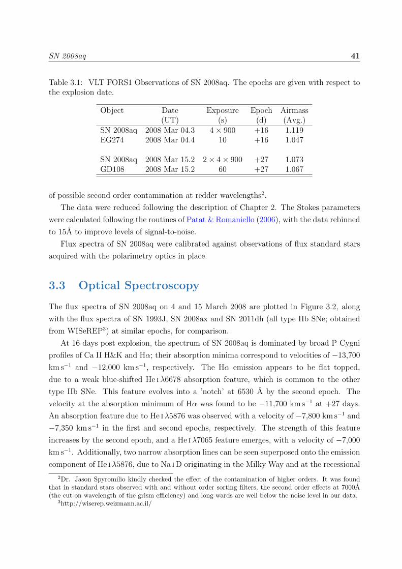
SN 2008aq 41
Table 3.1: VLT FORS1 Observations of SN 2008aq. The epochs are given with respect tothe explosion date.
Object Date Exposure Epoch Airmass(UT) (s) (d) (Avg.)
SN 2008aq 2008 Mar 04.3 4× 900 +16 1.119EG274 2008 Mar 04.4 10 +16 1.047
SN 2008aq 2008 Mar 15.2 2× 4× 900 +27 1.073GD108 2008 Mar 15.2 60 +27 1.067
of possible second order contamination at redder wavelengths2.
The data were reduced following the description of Chapter 2. The Stokes parameters
were calculated following the routines of Patat & Romaniello (2006), with the data rebinned
to 15A to improve levels of signal-to-noise.
Flux spectra of SN 2008aq were calibrated against observations of flux standard stars
acquired with the polarimetry optics in place.
3.3 Optical Spectroscopy
The flux spectra of SN 2008aq on 4 and 15 March 2008 are plotted in Figure 3.2, along
with the flux spectra of SN 1993J, SN 2008ax and SN 2011dh (all type IIb SNe; obtained
from WISeREP3) at similar epochs, for comparison.
At 16 days post explosion, the spectrum of SN 2008aq is dominated by broad P Cygni
profiles of Ca II H&K and Hα; their absorption minima correspond to velocities of −13,700
km s−1 and −12,000 km s−1, respectively. The Hα emission appears to be flat topped,
due to a weak blue-shifted He iλ6678 absorption feature, which is common to the other
type IIb SNe. This feature evolves into a ’notch’ at 6530 A by the second epoch. The
velocity at the absorption minimum of Hα was found to be −11,700 km s−1 at +27 days.
An absorption feature due to He iλ5876 was observed with a velocity of −7,800 km s−1 and
−7,350 km s−1 in the first and second epochs, respectively. The strength of this feature
increases by the second epoch, and a He iλ7065 feature emerges, with a velocity of −7,000
km s−1. Additionally, two narrow absorption lines can be seen superposed onto the emission
component of He iλ5876, due to Na iD originating in the Milky Way and at the recessional
2Dr. Jason Spyromilio kindly checked the effect of the contamination of higher orders. It was foundthat in standard stars observed with and without order sorting filters, the second order effects at 7000A(the cut-on wavelength of the grism efficiency) and long-wards are well below the noise level in our data.
3http://wiserep.weizmann.ac.il/

SN 2008aq 42
Figure 3.2: Flux spectra of SN 2008aq (shown in red) at 16 and 27 days post-explosion.Also shown are spectra of SN 1993J, SN 2008ax, and SN 2011dh (in black). All of thespectra are corrected for the recessional velocity of their respective host galaxies.

SN 2008aq 43
velocity of the host galaxy. The absorption observed around 8200 A is attributed to the Ca
II Infra-Red (IR) triplet, with a velocity of −12,000 km s−1 at 16 days post-explosion. The
Ca II IR triplet P Cygni profile is peculiar in that it exhibits a relatively deep absorption
paired with a weak emission component. Branch et al. (2002) noted that this behaviour
is characteristic of a ”detached” line forming region at velocities significantly greater than
that of the photosphere. By the second epoch, 10 days later, the velocity of the Ca II
IR triplet has decreased dramatically to a value of −9,000 km s−1 and the P Cygni profile
shows a prominent emission component. In the second epoch, the velocity of the Ca II IR
triplet and Ca H & K features has decreased more noticeably than that of other elements.
The most remarkable difference between SN 2008aq and the comparison SNe (see Figure
3.2) is the relative weakness of the He i features. In the first epoch (+16 days) the He iλ5876
line is much shallower in SN 2008aq than in SN 2008ax, SN 1993J or SN 2011dh. Also
the presence of a He iλ6678 feature can be inferred from the flat-topped profile of the Hα
emission component, whereas in SN 2008ax, SN 2011dh and SN 1993J, this feature is clearly
visible in the form of a ”notch.” In the second epoch (27 days post-explosion), the He i lines
of SN 2008aq have significantly increased in strength, but are still much weaker than in
the spectra of the other type IIb SNe, and Hα remains the dominant feature. Additionally,
the Ca II IR triplet feature at the second epoch is much shallower in the spectrum of SN
2008aq than in the spectra of 1993J, 2011dh and 2008ax, whereas at the first epoch the
strength of that feature is similar for SN 2008aq, SN 2008ax and SN 2011dh.
3.4 Spectropolarimetry
The polarisation and flux spectra for SN 2008aq are shown in Figure 3.3. Even before ISP
correction, the polarisation of SN 2008aq exhibits strong line features, particularly at +27
days.
3.4.1 Interstellar Polarisation
As described in Section 1.3.4 under the assumption of a Serkowski et al. type ISP the
maximum degree of polarisation can be constrained by Equation 1.11, where in the case
of an extra Galactic source the colour excess E(B − V ) used in the formula is the sum of
the colour excesses of the Milky and of the Host galaxy. An empirical relationship relating
the equivalent width of the sodium lines and the reddening was derived by Poznanski et al.
(2012). From the Na iD of the Milky Way component, we estimate that the reddening
associated with dust in our Galaxy is E(B − V )MW = 0.045 mag, which is in agreement

SN 2008aq 44
Figure 3.3: Scaled Flux spectra (brown) and polarisation spectra (blue) of SN 2008aq at16 days and 27 days post-explosion. The polarisation spectra were not corrected for inter-stellar polarisation. The regions highlighted in green were used to estimate the continuumpolarisation in Sections 3.4.2 and 3.4.2.

SN 2008aq 45
with the estimates of foreground reddening of E(B − V )MW = 0.04 mag by Schlafly &
Finkbeiner (2011)4. The reddening associated with the host galaxy was estimated from
the corresponding Na iD line, yielding E(B− V )host = 0.027 mag. Consequently, the total
reddening, is E(B − V )total = 0.072 mag, which is similar to the value found and used by
Stritzinger et al. (2009). The upper limit on the ISP associated with our data is therefore
0.65 percent.
To further characterise the ISP we make the assumption that the emission component
of Hα is intrinsically unpolarised at early times (Tran et al., 1997). It then follows that the
average polarisation over that feature must be representative of the ISP. Because the profile
of He i λ6678 is less apparent in the spectrum of SN 2008aq at +16 days, we favour the
Hα emission component of the first epoch for our ISP estimate. The values of the Stokes
parameters in the range 6700-6900 A we find qISP = 0.29 (± 0.07) percent and uISP = 0.13
(± 0.07) percent, corresponding to pISP = 0.32 (± 0.07) percent. This is well within the
upper limit derived from the Serkowski relation.
Using these estimates to correct for the ISP, we find a polarisation for SN 2008aq showed
in Figure 3.4. Before proceeding to the analysis, a number of caveats must be discussed.
Firstly, the profile of the degree of polarisation of SN 2008aq after ISP correction is
somewhat peculiar, particularly in the blue. Indeed, we expect line blanketing in the blue
and near-UV to lead to a strong dilution of the intrinsic polarisation, and so after ISP
removal we would expect p to decrease in this region of the spectrum, rather than increase
(as is clear when comparing the top panel of Figures 3.3 and 3.4).
Additionally, the assumption of complete depolarisation of strong emission lines is not
necessarily accurate (Tanaka et al., 2009). In particular, as mentioned in Section 3.3, the
flattened profile of the Hα emission component at +16 days indicates the presence of an
unresolved He i λ6678 absorption feature. Since absorption features are typically associated
associated with excess polarisation, this is an indication that our assumption of complete
depolarisation in the emission region of Hα may not be valid.
Unfortunately the lack of observation at earlier phases (where the Hα emission compo-
nent may be less contaminated by He i λ6678) means that it is not possible at this time to
check the veracity of our ISP estimate any further.
Consequently our derived ISP values should be considered with great caution and the
following analysis is performed both on the corrected and uncorrected data sets.
4https://ned.ipac.caltech.edu/

SN 2008aq 46
Figure 3.4: Scaled Flux spectra (brown) and polarisation spectra (blue) of SN 2008aq at16 days and 27 days post-explosion. The polarisation spectra were corrected for interstel-lar polarisation. The regions highlighted in green were used to estimate the continuumpolarisation in Sections 3.4.2 and 3.4.2.

SN 2008aq 47
3.4.2 Line and Continuum polarisation
+16 days
At the first epoch, the uncorrected polarisation data are dominated by a large feature
starting at 5330A with an initial polarisation of p∼0.5 percent, rising to a 1.24±0.15 percent
peak at 6168A, and decreasing back down to the ∼0.1 percent level at 6430A. This feature
can be interpreted as a blend of Hα and He iλ5876 with the main peak being correlated to
the Hα absorption component, as has been seen previously in type IIb SNe (e.g. Mauerhan
et al. (2015)).
In the ISP corrected data this broad feature is not seen, and the polarisation is roughly
constant at ∼0.5 percent. A narrow peak is seen at 5587A with p = 0.96 ± 0.15 percent,
which could be associated with a high velocity (−14, 500 km s−1) component of He i λ5876
although it is unclear why the polarisation would settle back down to 0.5 percent and remain
constant across the main absorption and emission components of the P Cygni profile. The
Hα peak is found in the same location as in the ISP uncorrected data (6178A), and with
a polarisation p = 1.01± 0.15 which is within uncertainties of the uncorrected value.
Another feature visible at +16 days after explosion, albeit more subtle, is the polarisa-
tion peak at 3772A associated with the absorption minimum of the large Ca H&K feature.
The peak reaches a polarisation of p = 0.79 ± 0.37 percent in the uncorrected data and
p = 0.99± 0.38 in the ISP corrected data.
In the red, the high levels of noise beyond ∼7900 A caused by fringing make the in-
terpretation of the polarisation associated with the absorption feature of the Ca IR triplet
difficult. In particular it should be noted that the isolated peaks at 7630, 8005, 8350, and
8410 A are outliers and not representative of a true signal (see Section A.2). There may be
a hint of polarisation excess correlated with the absorption component of the Ca IR triplet,
but values of peak polarisation cannot be accurately derived.
The continuum polarisation of SN 2008aq was evaluated by producing the average of
the polarisation measured in a wavelength range identified as devoid of strong lines. We
chose the spectral region extending from 7650 to 7900A (highlighted in green in Figures
3.3 and 3.4), avoiding strong telluric lines and the onset of the Ca II IR region. In this
first epoch, the continuum polarisation is estimated at p = 0.22± 0.12 percent in the ISP
corrected data and p = 0.34± 0.14 percent for the uncorrected data. Within uncertainties,
these two values are the same, and correspond to an axis ratio of ∼0.90 (Hoflich 1991 –
their figure 4).

SN 2008aq 48
+27 days
The evolution of the polarisation by 27 days after explosion is drastic, and shows features
that are less blended and have stronger amplitudes, both in the ISP corrected and ISP
uncorrected data. The He i λ5876 and Hα are now separate. The helium peak is found
at 5722 A and p = 2.21 ± 0.11 percent (p = 2.26 ± 0.13 percent) for the ISP uncorrected
(corrected) data. Hydrogen on the other hand shows a relatively flat peak between 6040
and 6210A; averaging the polarisation in this wavelength range we find p = 1.62 ± 0.10
percent and p = 1.66±0.11 percent in the ISP uncorrected and corrected data, respectively.
Additionally, a clear He i λ7065 feature is now found at 6882A with a peak polarisation
of p = 1.60 ± 0.12 percent (p = 1.71 ± 0.14 percent) in the ISP uncorrected (corrected)
data.
As opposed to the first epoch, the calcium infrared triplet now clearly dominates over
the noise, and has become the strongest polarisation feature. The infrared calcium peak is
found at 8251A with p = 3.3± 0.3 percent in both the ISP corrected and uncorrected data
sets. The Ca H&K feature on the other hand, has not significantly strengthened, with a
peak now reaching p = 0.97± 0.45 percent (p = 1.31± 0.45 percent) at 3787A in the ISP
uncorrected (corrected) data set.
Lastly, the continuum polarisation is calculated in the same way as for epoch 1, and is
found to be p = 1.36 ± 0.10 percent / p = 1.33 ± 0.140 percent for the ISP corrected and
uncorrected data, respectively. This increase in polarisation indicates a significant decrease
in axis ratio, which is now ∼0.77 (Hoflich 1991 – their figure 4).
3.4.3 q − u plots
Firstly we present in Figure 3.5 the q−u plots for the spectropolarimetric data of SN 2008aq
across the full wavelength range. The dominant axis is fitted using an ODR method as
described in Section 2.3.5.
At +16 days the data shows a subtle elongation. This is expected for low global asym-
metry (Wang & Wheeler, 2008) and is therefore consistent with the low axis ratio deter-
mined in Section 3.4.2. The angle of the dominant axis (calculated anti-clockwise from the
u = 0 line) is 61 ± 2◦in the uncorrected data and 63 ± 2◦in the ISP corrected data. At
+27 days, the elongation is more pronounced and the angle of the dominant axis is found
to be 113 ± 1◦(112 ± 1◦) for the ISP uncorrected (corrected) data. A global rotation of
52◦(49◦) is therefore observed between the ISP uncorrected (corrected) data at +16 days
and +27 days, which corresponds to a polarisation angle (P.A) rotation of 26◦(24.5◦), from

SN 2008aq 49
Figure 3.5: Spectropolarimetric data of SN 2008aq presented on q − u plots. The toppanels show the data at +16 days post-explosion while the data at +27 days are shownon the bottom panels. The left hand side panels show the ISP uncorrected data while theright hand side panels show the ISP corrected data. The colour bar represents wavelength,and the dashed line shows the dominant axis of the data as determined with OrthogonalDistance Regression.

SN 2008aq 50
∼30.5◦(31◦) at +16 days to 56.5◦(56◦) at +27 days.
The spectropolarimetric data of SN 2008aq in the region of Ca H&K λ3948, He i λ5876,
Hα, He i λ7065 and Ca ii λ8567 are shown in Figure 3.6 and 3.7 for the ISP uncorrected
and corrected case, respectively.
At the first epoch we find that only the Ca H&K and the Hα polarisation show significant
departure from the rest of the data. Their orientation off-axis with respect to the dominant
axis indicates the presence of small scale asymmetries that can be caused by clumping. At
+27 days post-explosion all of the plotted lines show features on the q − u plot. The Ca
H&K and He i λ7065 features are both very narrow and therefore quite subtle, but their
peak polarisation correspond to significant departures from the dominant axis, suggesting
asymmetrically distributed line forming regions.
The He i λ5876 loop at +27 days is very well defined and is the consequence of a
change in the sky projected location of the line forming region with velocity (i.e. depth). A
similar interpretation is consistent with the Hα polarisation feature, although the chirality
is reversed compared to the helium feature (clockwise in He i and anti-clockwise in Hα).
Additionally the loop is more extended suggesting greater geometry changes with depth.
Finally the Ca ii IR feature shows an extended and complex polarisation feature that
roughly follows the dominant axis. The complexity of the loop may reflect the complexity
of the geometry of the line forming region in 3D, although this interpretation should be
considered with caution given the size of the error bars.

SN 2008aq 51
Figure 3.6: Uncorrected spectropolarimetric data associated with the strong spectral linesof SN 2008aq. The colour bars represent the velocity space corresponding to each line. Thedominant axis is plotted as the dashed line and the light grey points show the whole datafor reference.

SN 2008aq 52
Figure 3.7: ISP corrected spectropolarimetric data associated with the strong spectral linesof SN 2008aq. The colour bars represent the velocity space corresponding to each line. Thedominant axis is plotted as the dashed line and the light grey points show the whole datafor reference.

SN 2008aq 53
3.5 Discussion & Conclusion
Optical spectra and spectropolarimetric data of SN 2008aq were presented at 2 epochs: 16
days and 27 days post-explosion. The intrinsic polarisation calculated for SN 2008aq at
+16 days (pcont= 0.22 ± 0.12 percent ) is much lower than found in other type IIb SNe at
earlier and similar epochs: e.g. SN 2008ax at +9 days (pcont= 0.64 ± 0.02 percent) and SN
2011dh at +14 days (pcont ∼ 0.5 percent – (Chornock et al., 2011; Mauerhan et al., 2015)).
By the second epoch, the continuum polarisation of SN 2008aq had reached a value of
pcont=1.33 (± 0.33) percent, which is similar to the continuum polarisation calculated for
SN 1993J at +29 days (pcont ∼ 1 percent) and that of SN 2001ig at 31 days (∼1 percent –
Tran et al. 1997; Maund et al. 2007).
A characteristic of type IIb SNe is the increase in strength of their He features with time,
as they transition to type Ib SNe. This behaviour is observed in SN 2008aq (see Section
3.3), however, comparison with other type IIb SNe at similar epochs reveals that the He
features in the spectra of SN 2008aq are significantly weaker (see Figure 3.2). Additionally,
we find that the pseudo equivalent width of the He iλ5876 absorption component at both
epochs was roughly 4 to 5 times smaller in SN 2008aq than in other type IIb SNe (Liu
et al., 2016). The scarcity of helium indicates that the receding photosphere of SN 2008aq
reached the helium layer at a later date than in SN2008ax, SN 2011dh, SN 1993J, and
other previously studied type IIb SNe; this may suggest that the progenitor of SN 2008aq
was less stripped than other type IIb SNe.
Similarly to SN 2001ig (Maund et al., 2007), SN 2008aq showed a drastic dominant
axis rotation between +16 and +27 days (see Figure 3.5) suggesting a change in the axis
of symmetry deeper into the envelope. Additionally, as we have seen in Section 3.4.3,
departures from axial symmetry are seen at both epochs, as indicated by the presence of
loops in the q− u plots of CaH&K and Hα at +16 days, and in the q− u plots of calcium,
Hα, He i λ5876 and He i λ7065 at +27 days after explosion. Therefore, both the overall
geometry and smaller scale geometry of the envelope of SN 2008aq vary with depth.
As mentioned in Section 3.4.1, our determination of the ISP is dependent on the assump-
tion that the Hα P Cygni profile at early times is completely depolarised (e.g. Trammell
et al. 1993, Tran et al. 1997). Given the suspected contamination of the Hα emission by He i
λ6678, this assumption is to be taken with great caution. On the whole, the interpretation
of the data is mostly unchanged whether we consider the ISP removed or uncorrected data
as the continuum polarisation values and the q − u plot features are all consistent. The
only major change between the ISP corrected and uncorrected data is the profile of the
polarisation spectrum at +16 days (see the top panels of Figure 3.3 and 3.4). The shape

SN 2008aq 54
of the ISP corrected data being a lot more difficult to interpret, it either suggests the need
for a novel interpretation, or simply be a reflection of the inaccurate ISP removal. Given
the current context, the latter explanation seems more likely. Additionally, since this work
studies the variations of the polarisation across the lines, the absolute value of the derived
polarisation is of interest but not critical to our conclusions.
In the next chapter we will focus on another type IIb SN: SN 2011hs.

Chapter 4
The 3D shape of Type IIb SN 2011hs
55

SN 2011hs 56
4.1 Introduction
Type IIb SNe are better represented than other types in the spectropolarimetric literature,
and the previous chapter on SN 2008aq added a new object to our sample. However, the
number of high-quality multi-epoch data sets remains limited (5 SNe, including SN 2008aq
– see Table 1.1). Increasing our sample is ultimately necessary to compare the statistical
distribution of the observed polarisation to available models (e.g. Hoflich 1991; Kasen
et al. 2003; Dessart et al. 2011; Tanaka et al. 2017). In this chapter we analyse the data
for another type IIb SN: SN 2011hs. We present 7 epochs of spectropolarimetry, from −3
days to +40 days with respect to V-band maximum. This, along with SN 2011dh, is one
of the best data sets ever obtained for a type IIb SN, in terms of time coverage, cadence
and signal-to-noise. In Section 4.2 we give the details of the observations. In Section 4.3 a
thorough analysis of the interstellar polarisation is provided, and we present the intrinsic
polarisation of SN 2011hs in Section 4.4. The results are discussed and compared to the
literature in Section 4.5, and we summarise the results in Section 4.6.
This work has been published in the Monthly Notices of the Royal Astronomical Society
(Stevance et al., 2019).
4.2 Observations and data reduction
SN 2011hs was discovered by Stuart Parker on 12.476 November 2011 and classified by
Milisavljevic et al. (2011). It is located at R.A. = 22h57m11s and δ = -43◦23’04” in the
galaxy IC 5267 (face-on sA0) with redshift z = 0.005711, corresponding to a recessional
velocity of 1714 km s−1(Koribalski et al., 2004). A series of spectropolarimetric obser-
vations of SN 2011hs were taken at the VLT with FORS2 (ESO ID program 088.D0761;
PI: J. Maund). Linear spectropolarimetry was obtained for 4 half-wave retarder angles
(0◦, 22.5◦, 45◦, 67.5◦) at seven epochs between 19 November 2011 and 01 January 2012.
A summary of observations is given in Table 4.1. All observations were performed with
the 300V grism, providing a spectral resolution of 12 A. The GG435 order sorting filter
was used to avoid contamination of our data by higher spectral orders. Our data are thus
limited to the wavelength range 4450A – 9330A. The data were reduced as described in
Chapter 2. The data acquired on 19 November, 24 November and 02 December 2011 were
binned to 15 A, the data captured on 10 December 2011 were binned to 30A and the data
obtained for subsequent dates were binned to 45 A to increase the signal-to-noise ratio.
The spectra were flux calibrated using the standard stars reported in Table 4.1 in order
to remove the instrumental response. It should be noted, however, that due to unknown

SN 2011hs 57
Table 4.1: VLT Observations of SN 2011hs. The epochs are given relative to the estimatedV-band maximum.aFlux Standard.
Object Date Exp. Time Epoch Airmass(UT) (s) (days)
SN 2011hs 2011 Nov. 19 8 × 850 −3 1.05− 1.23EGGR 141a 2011 Nov. 19 2×60 − 1.26
SN 2011hs 2011 Nov. 24 8 × 900 +2 1.1− 1.36EGGR 150a 2011 Nov. 24 2 × 191 − 1.31
SN 2011hs 2011 Dec. 02 8 × 900 +10 1.16− 1.56LTT1788a 2011 Dec. 02 2 × 60 − 1.04
SN 2011hs 2011 Dec. 10 8 × 900 +18 1.3− 2.0LTT1788a 2011 Dec. 10 2 × 60 − 1.8
SN 2011hs 2011 Dec. 16 4 × 855 +24 1.4− 2.3LTT1788a 2011 Dec. 16 2 × 120 − 1.14
SN 2011hs 2011 Dec. 23 4 × 1100 +31 1.4− 1.77LTT1788a 2011 Dec. 23 2 × 60 − 1.034
SN 2011hs 2012 Jan. 01 4 × 1100 +40 1.6− 2.1LTT1788a 2011 Dec. 16 2 × 120 − 1.14

SN 2011hs 58
Epoch Fe ii
−3 days −9,860 km s−1
+2 days −8,760 km s−1
+10 days −6,320 km s−1
+18 days −5,570 km s−1
+24 days −5,390 km s−1
+31 days −4,810 km s−1
+40 days −4,470 km s−1
Table 4.2: Line velocities at the absorption minimum for Fe ii λ5169 at all epochs, whichis used as a proxy for photospheric velocity.
wavelength dependent slit losses, absolute flux calibration was not possible.
4.2.1 Observed flux and spectropolarimetry
Flux spectrum and photospheric velocity
In Figure 4.1, we present the observed spectropolarimetry and flux spectrum at seven new
epochs for SN 2011hs.
As noted by Bufano et al. (2014), early epochs of spectroscopy are dominated by Hα
(−3 days), but as the supernova evolves through maximum the feature decreases in strength
and a blue shoulder appears (+2 days). We also see that from a week after maximum, the
spectrum is dominated by He i features. An exhaustive spectroscopic analysis is beyond the
scope of this chapter, and more details on the spectroscopy of SN 2011hs and comparison
to other SNe can be found in Bufano et al. (2014). Nonetheless, for the needs of this work
we estimate the photospheric velocities at the time of observations (see Section 4.4). The
velocities of the Fe ii lines in the blue part of the spectrum can be used as a proxy to probe
photospheric velocity (e.g. Bufano et al. 2014), so we perform fits of Fe ii λ5169 at all
epochs in order to find the absorption minima. The resulting velocities are given in Table
4.2, and are consistent with the estimates of Bufano et al. (2014) from fits of the same line,
see their figure 9. Note that errors are not provided because the formal uncertainties on
these values resulting from the Gaussian fits would be misleadingly small. The main source
of error here would be from the blending of multiple lines, which is not taken into account.
Consequently, the values provided in Table 4.2 should be used with caution.

SN 2011hs 59
Figure 4.1: Flux spectrum (black) and degree of polarisation (not corrected for ISP -orange) of SN 2011hs ranging from −3 days to +40 days. The grey shaded areas representthe regions affected by telluric lines. The data at −3, +2 and +10 days were binned to15A, the data at +18 days were binned to 30A and the following epochs were binned to45A. Note that the strong peaks of polarisation near 4600A and 5700A at +31 and +40days are not considered to be real (see Section 4.2.1).

SN 2011hs 60
Observed polarisation
As seen in Figure 4.1, we detect significant polarisation in the direction of SN 2011hs,
showing an underlying slope with a higher degree of polarisation at the blue end of the
spectrum (∼3 percent) than at the red end (∼1 percent). This behaviour is not expected
for the continuum polarisation of SNe since Thomson scattering is wavelength independent.
Additionally, some excess polarisation is associated with the absorption component of Ca ii
from 10 days after V-band maximum, and polarisation troughs are seen corresponding to
Hα at the first 3 epochs, as well as with He λ5876 at +10 and +18 days. The presence of
troughs is inconsistent with the expected correlation of polarisation peaks with absorption
components (e.g. Wang & Wheeler 2008). These discrepancies seem to indicate that in-
terstellar polarisation contributes very significantly to the continuum polarisation observed
(see Section 4.3 for a more complete discussion).
Lastly, it should be noted that the strong peaks near 4600A and 5700A at +31 and
+40 days are coincident with significant variations from zero in our instrumental signature
correction ∆ε (see Maund 2008), reducing our confidence in our data at these wavelengths.
We therefore do not consider these peaks to be real.
4.3 Interstellar polarisation
4.3.1 Galactic ISP
In order to estimate the contribution of the Galactic ISP we searched for Milky Way field
stars in the vicinity of SN 2011hs. If we assume that they are intrinsically unpolarized,
any polarisation measured for these stars is due to Galactic ISP. In the Heiles (2000)
catalogue, we found two stars within 2 degrees of SN 2011hs: HD218227 and HD215544
with polarisation p = 0.012 and p = 0.116 percent, respectively. Using the parallaxes found
in the Gaia data release DR2 (Luri et al., 2018) we calculate distances of 36.1±0.7 pc and
501±10 pc for HD218227 and HD215544, respectively. HD218227 being such a nearby
object explains its low polarisation degree compared to HD215544, and the latter better
samples the Galactic dust column and the ISP in the direction of SN 2011hs.
It is possible to put an upper limit on the Galactic ISP following Eq. 1.11. The Galactic
reddening in the direction of SN 2011hs is E(B-V)= 0.011± 0.002 (Schlafly & Finkbeiner,
2011), yielding pISP < 0.099± 0.018 percent. The polarisation of HD215544 is at the upper
end of this limit (within uncertainties). This is much lower than the observed polarisation
and the Galactic ISP is therefore a small contribution to the total observed ISP.

SN 2011hs 61
Figure 4.2: Stokes parameters q and u at +40 days (dark blue; errors in light blue) 3σ-clipped according to ∆ε; the discarded points are shown in orange. The bin size for thedata is 3.3A. The fits to the σ-clipped data are shown in magenta.
4.3.2 ISP determination from late time data
In order to estimate the ISP from our observations, some assumptions must be made.
Any such estimate is inevitably model dependent. In the context of electron scattering
by the SN ejecta, at late times the polarisation intrinsic to the SN will tend towards zero
since the electron density decreases as the ejecta expand, and the observed polarisation
therefore tends to the ISP. By assuming complete depolarisation at our last epoch (+40
days) and fitting a straight line to the normalised Stokes parameters q and u, the wavelength
dependent qISP and uISP can then be found (see Figure 4.2). Best results were obtained
when using the original data at +40 days (not rebinned to 45A), where spurious points
were removed according to their corresponding ∆ε. Data points whose ∆ε showed a 3σ or
greater deviation from zero were not included in our fits.
The resulting ISP-wavelength relationships are:
qISP (percent) = 2.63(±0.19)× 10−4 × λ− 2.68(±0.14), (4.1)
uISP (percent) = 3.61(±0.17)× 10−4 × λ− 3.94(±0.12), (4.2)

SN 2011hs 62
where λ is in A, the gradients have units of A−1 and the intercepts are unit-less. The
reduced chi-squared (χ2ν) values on the q and u fits were 1.39 and 0.93, respectively. The
fits are therefore satisfactory and the derived wavelength dependent relationships for q and
u were used to retrieve the intrinsic polarisation of SN 2011hs presented and analysed in
Section 4.4.
4.3.3 Host galaxy of SN 2011hs and Serkowski law
From the upper limits on the Galactic ISP derived in Section 4.3.1 we can conclude that
most of the ISP in the data of SN 2011hs originated from IC 5267. Under the assumption
that the size and composition of interstellar dust grains are similar in the host galaxy of
SN 2011hs as to those in the Milky Way, the Serkowski limit pISP < 9 × E(B − V ) can
be applied to derive a value for the maximum pISP. In order to do so, a value for the
reddening of IC 5267 must be calculated. To this end, we measured and averaged the
equivalent widths of the Na i D line in the data of epochs 1 to 3 (at later epochs the blend
of sodium with He i made our equivalent width measurements unreliable). We then used
the relationship between equivalent width and reddening described by Poznanski et al.
(2012), and calculated E(B − V )host = 0.11 (±0.02). According to Eq. 1.11, this yields
pISP < 1.09 (±0.18). At 5000 A, however, we find pISP = 2.50(±0.15) percent, as calculated
from qISP and uISP derived in Section 4.3.2. Therefore, the assumption that the dust of IC
5267 or in the vicinity of SN 2011hs is similar to that of the Milky Way may not be correct.
It is however worth noting that the Na i D lines are caused by discrete gas clouds and do not
probe the more diffuse ISM, therefore only providing a lower limit on the dust extinction.
Consequently, the Poznanski et al. (2012) estimate may not be completely adequate.
Another approach is to fit our data at +40 days with the Serkowski law (see Eq. 1.10).
We attempted to find new values of the parameters pmax and λmax by minimising the χ2
to better fit our data. Two forms of the constant K were considered: the original value
derived by Serkowski et al. (1975) KS = 1.15, and the λmax dependent form of Whittet
et al. (1992) KW = 0.01 + 1.66λmax.
The normalised Stokes parameters q and u can be expressed as functions of the wave-
length dependent degree of polarisation p(λ) and the polarisation angle θ as
q = p(λ) cos(2θ) and u = p(λ) sin(2θ), (4.3)
where p(λ) is defined by Eq. 1.10 and here θ = 120◦ (as from Eqs. 4.1 and 4.2 the
polarisation angle θ is found to be 120◦±2◦ across our wavelength range). Note that we
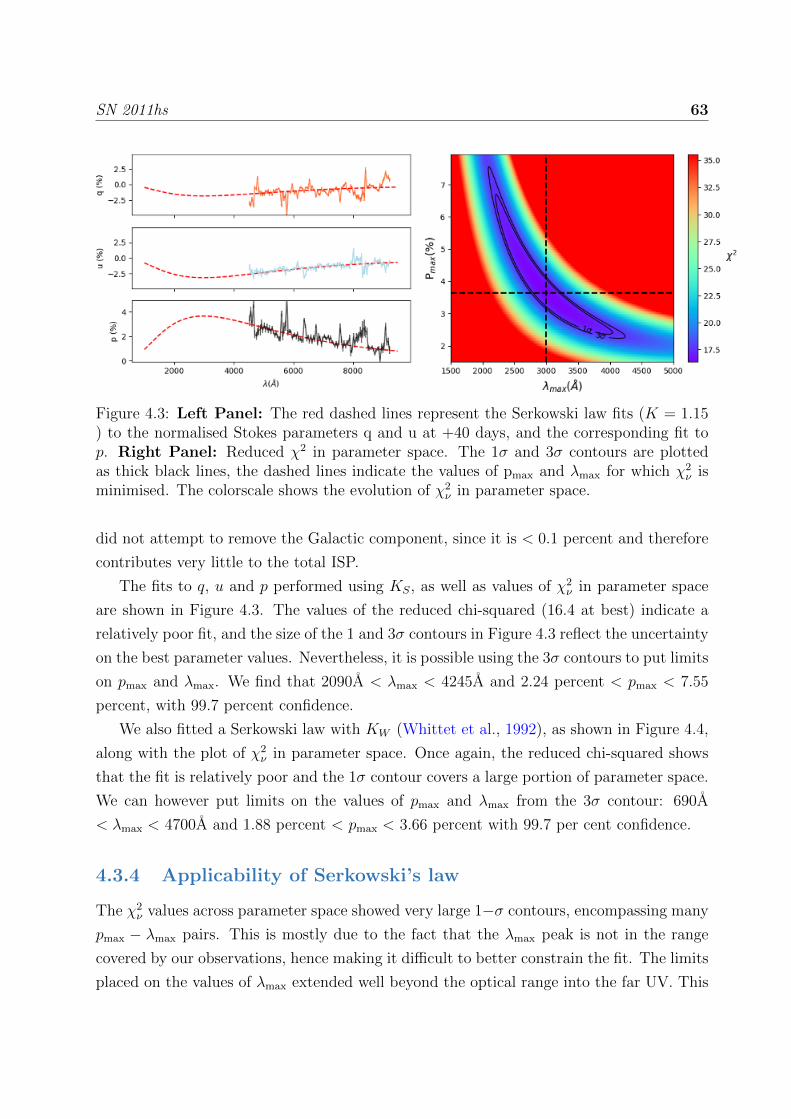
SN 2011hs 63
Figure 4.3: Left Panel: The red dashed lines represent the Serkowski law fits (K = 1.15) to the normalised Stokes parameters q and u at +40 days, and the corresponding fit top. Right Panel: Reduced χ2 in parameter space. The 1σ and 3σ contours are plottedas thick black lines, the dashed lines indicate the values of pmax and λmax for which χ2
ν isminimised. The colorscale shows the evolution of χ2
ν in parameter space.
did not attempt to remove the Galactic component, since it is < 0.1 percent and therefore
contributes very little to the total ISP.
The fits to q, u and p performed using KS, as well as values of χ2ν in parameter space
are shown in Figure 4.3. The values of the reduced chi-squared (16.4 at best) indicate a
relatively poor fit, and the size of the 1 and 3σ contours in Figure 4.3 reflect the uncertainty
on the best parameter values. Nevertheless, it is possible using the 3σ contours to put limits
on pmax and λmax. We find that 2090A < λmax < 4245A and 2.24 percent < pmax < 7.55
percent, with 99.7 percent confidence.
We also fitted a Serkowski law with KW (Whittet et al., 1992), as shown in Figure 4.4,
along with the plot of χ2ν in parameter space. Once again, the reduced chi-squared shows
that the fit is relatively poor and the 1σ contour covers a large portion of parameter space.
We can however put limits on the values of pmax and λmax from the 3σ contour: 690A
< λmax < 4700A and 1.88 percent < pmax < 3.66 percent with 99.7 per cent confidence.
4.3.4 Applicability of Serkowski’s law
The χ2ν values across parameter space showed very large 1−σ contours, encompassing many
pmax − λmax pairs. This is mostly due to the fact that the λmax peak is not in the range
covered by our observations, hence making it difficult to better constrain the fit. The limits
placed on the values of λmax extended well beyond the optical range into the far UV. This

SN 2011hs 64
Figure 4.4: Left Panel: The red dashed lines represent Serkowski law fits (K = 0.01 +1.66λmax) to the normalised Stokes parameters q and u at +40 days, and the correspondingfit to p. Right Panel: Reduced χ2 in parameter space. The 1σ and 3σ contours areplotted as thick black lines, the dashed lines indicate the values of pmax and λmax for whichχ2ν is minimised. The colorscale shows the evolution of χ2
ν in parameter space.
is a concern as Serkowski’s law was empirically defined from optical data (Serkowski et al.,
1975), and it has been found that the law is not necessarily applicable in the UV (e.g.
Anderson et al. 1996; Martin et al. 1999; Patat et al. 2015). Furthermore Martin et al.
(1999) explain that the Serkowski equation (see Eq. 1.10) is not flexible enough to provide
adequate fits all the way from UV to IR for a given K, and that, often, performing a three
parameter fit to find pmax, λmax and K gives better results. Patat et al. (2015) applied this
method, and for the case of SN 2006X found K = 1.47± 0.05, which is very different from
KW and KS which we used for our fits. Therefore, fitting data which peak in the UV with
optical Serkowski laws as is done here may not be adequate.
The very different shapes of the χ2ν contours in parameter space for the two values of K
used in this work (see Figures 4.3 and 4.4) shows the importance of the choice of K. Given
the nature of our data, in particular the fact that λmax is visibly outside of the range we
cover, a three parameter fit cannot help constrain our estimate of the parameters.
On the whole, the observed polarisation curves are very different from what is expected
from Galactic type ISP. Furthermore, it is anticipated that the ISP P.A. should be parallel
to the local spiral arm of the host galaxy at the location of the SN, due to the alignment
of the dust with the magnetic field of the host. However, the ISP angle of ∼120◦ is found
not to be parallel to the local spiral arm (see Figure 4.5). This could suggest that the dust
in IC 5267 or in the local neighbourhood of SN 2011hs may be different from that in the
Milky Way.

SN 2011hs 65
Figure 4.5: Orientation of the ISP polarisation angle at the location of SN 2011hs (markedby the star) in IC 5267. The image of the host galaxy is a B, V, R, I composite from theCarnegie-Irvine Galaxy Survey (CGS – Ho et al. 2011).
An alternative explanation to the observed ISP profile and P.A. is the presence of
circumstellar dust. Polarisation curves increasing towards short wavelengths and with
λmax < 4000 A have been see in type Ia SNe (e.g. 1986G, SN 2006X, SN 2014J – Patat
et al. 2015). Hoang (2017) modelled the observed polarisation curves and extinction and
found this behaviour to be the result of an enhancement in small silicate grains in the
dust. They suggest this could be due to cloud-cloud collisions resulting from SN radiation
pressure. Alternatively Hoang et al. (2018) show that large silicate grains can be destroyed
by large radiation fields such as those around massive stars and SNe. Additionally, Cikota
et al. (2017), remarked that the polarisation curves of type Ia SNe are similar to those
of proto-planetary nebulae, whose polarisation curves are produced by scattering in the
circumstellar medium. Consequently, the peculiar ISP found in the observations of SN
2011hs may hint at the presence of circumstellar dust around SN 2011hs.
4.4 Intrinsic polarisation
The degree of polarisation of SN 2011hs after ISP correction (see Section 4.3) is shown
alongside the flux spectra in Figure 4.6.

SN 2011hs 66
Figure 4.6: Degree of polarisation (corrected for ISP) of SN 2011hs ranging from −3 daysto +40 days (purple). The flux spectrum is shown in black, the light grey shaded areashighlight the regions of telluric lines, and the green horizontal lines show the wavelengthranges used to calculate the continuum polarisation. The data at −3, +2 and +10 dayswere binned to 15A, the data at +18 days was binned to 30A and the following epochswere binned to 45A. Note that the strong peaks of polarisation near 4600A and 5700A at+31 and +40 days are not considered to be real (see Section 4.2.1).

SN 2011hs 67
Table 4.3: Summary of the polarisation and polarisation angle (P.A.) of the continuumand strong lines of SN 2011hs by epoch.
Epoch p in percent (wavelength range) P.A.
Continuum−3 days 0.55 ± 0.12 (6955-7115 / 7225-7530 / 7655-7840) 170◦±7◦
+2 days 0.75 ± 0.11 (6960-7140 / 7250-7425 / 7700 -7850) 158◦±4◦
+10 days 0.48 ± 0.09 (7055-7130 / 7350-7415 / 7790-7930) 141◦±7◦
+18 days 0.29 ± 0.18 (7310-7535 / 7800-7925) 120◦±9◦
He iλ5876−3 days 0.59 ± 0.05 (5590-5670) 173◦±8◦
+2 days 0.89 ± 0.03 (5660-5715) 155◦±4◦
+10 days 0.57± 0.05 (5685-5771) 141◦±10◦
+18 days 1.08 ± 0.36 (5712) 54◦±3◦
Hα−3 days 0.75 ± 0.08 (6070-6200) 5◦±6◦
+2 days 0.89 ± 0.10 (6085-6160) / 0.87 ± 0.08 (6225-6295) 167◦±1◦/ 168◦±3.4◦
+10 days 0.62 ± 0.02 (6150-6200) / 0.59 ± 0.01 (6285-6305) 155◦±3◦/ 163◦±1◦
Ca ii−3 days 1.17± 0.20 (8030-8180) 177◦±4◦
+2 days 1.25± 0.15 (8055-8250) 166◦±4◦
+10 days 1.20± 0.25 (8275-8375) 134◦±7◦
+18 days 1.35± 0.30 (8205-8415) 134◦±13◦
+24 days 1.30± 0.26 (8100-8400) 75◦±23◦
+31 days 1.79± 0.22 (8100-8300) 41◦±18◦
+40 days 1.64± 0.16 (8100-8300) 107◦±19◦

SN 2011hs 68
We derived the degree of polarisation and P.A. for the prominent polarisation features
and the continuum where possible. Each value is associated with a particular wavelength
or wavelength range. In the former case, we simply recorded the polarisation at the corre-
sponding wavelength bin, whereas when a range is provided we averaged the values within
that range and used the standard deviation as the error. In order to estimate the contin-
uum polarisation, we average the polarisation values in spectral regions devoid of strong
lines and telluric lines. We could only find suitable regions of the spectra in epochs 1 to
4, and the wavelength ranges considered are indicated by the green lines in Figure 4.6.
The precise ranges used, and the continuum polarisation and P.A. derived can be found in
Table 4.3.
The continuum polarisation is found to be constant within errors at epochs 1 and 2,
with p = 0.55± 0.12 percent and p = 0.75± 0.11 percent, respectively. At those dates the
P.A. of the continuum is also constant within error (170◦± 7◦and 158◦± 4◦at −2 and +3
days, respectively). The degree of polarisation then decreases to p = 0.48 ± 0.09 percent
by +10 days and p = 0.29 ± 0.18 percent by +18 days, and a significant rotation of the
P.A. is also observed (141◦± 7◦and 120◦± 9◦at +10 and +18 days, respectively).
Prominent polarisation features of Heλ5876 are seen in Figure 4.6 from −3 days to +18
days with degree of polarisation as high as p = 1.08±0.36 percent at the latter epoch. The
P.A. of helium follows that of the continuum at the first 3 epochs (see Table 4.3), but a
sudden ∼90◦rotation is seen from +10 days to +18 days (from 141◦to 54◦, respectively).
The Hα polarisation at −3 days and +2 days exhibits a very broad feature extending
from ∼5700A to ∼6300A. The broad hydrogen profile rises to p = 0.75 ± 0.08 percent
in the first epoch (see Figure 4.6 and Table 4.3). By +2 days two distinct peaks can be
seen centred around 6125A and 6260A, which share the same degree of polarisation within
errors (p = 0.89 ± 0.10 percent and p = 0.87 ± 0.08 percent, respectively). These two
peaks become better defined at +10 days, as the underlying broad profile fades, although
their amplitude is seen to decrease by ∼0.3 percent with respect to epoch 2. In subsequent
epochs, no significant hydrogen feature is detected above the noise. Over time Hα exhibits
a decrease in P.A., as seen in helium and the continuum.
Calcium shows by far the most prominent polarisation features at all epochs, and is the
only element to continue exhibiting polarisation above noise levels up to our last epoch at
+40 days (see Figure 4.6 and Table 4.3). The amplitude of the feature remains roughly
constant from −3 days to +24 days, between 1 and 1.5 percent, although the P.A. is seen
to slowly decrease over time. In the last two epochs, however, the polarisation degree is
well above the 1.5 percent level, and a change in the evolution of the P.A. is also seen, as

SN 2011hs 69
between +31 days and +40 days it increases by ∼60◦.
4.4.1 Polar Plots
To help visualise the behaviour of the P.A. in velocity space, we create polar plots, which
are diagrams showing the relative positions of the P.A. associated with strong polarisation
features. They were first proposed by Maund et al. (2009), and use the radial velocity
position and the angle on the plane of the sky as coordinates. In Figure 4.7 we show the
polar plots at all epochs for helium, hydrogen and calcium. Note that the data were binned
for better visualisation; the centres of the bins are the average P.A. calculated within the
range. The angular extent of the bin on the polar plot represents the error, so that a larger
angular extent shows greater uncertainty on the P.A. for a particular line, not a greater
physical extent.
The locations of the continuum shown on Figure 4.7 for epochs 1 through 4 correspond
to the polarisation angles calculated for the continuum values given in Table 4.3. Unfor-
tunately the continuum polarisation could not be formally calculated at the last 3 epochs,
since we could not isolate spectral regions devoid of strong lines. We attempted to estimate
the polarisation angle of the continuum by identifying its possible locus in q− u space (see
Section 4.4.2 and Figure 4.8) by using a 2-σ clipping method to eliminate outliers and the
contribution of strong lines. This method was successfully used for the data at +24 and
+31 days, yielding angles of 99◦±39◦and 98◦±25◦, respectively. This is consistent with
an absence of rotation from +18 days to +24 and +31 days. At the last epoch, the av-
erage values of q and u and their standard deviations are consistent with null continuum
polarisation.
The change in P.A. of the continuum described in the previous section is visualised as a
progressive clockwise rotation that takes place at epochs 2 to 4. Additionally, the P.A. of
helium, hydrogen and calcium clearly follow the clockwise rotation of the continuum over
time, apart from Heλ5876 at +18 days. In Section 4.4 we highlighted the 90◦rotation of
this feature from +10 days to +18 days. This behaviour is clearly seen in Figure 4.7, as
at +18 days the Heλ5876 bins now fall into the upper quadrant, when the helium data
were located in the bottom quadrant at +2 and +10 days. It is also very distinct from the
behaviour of the other line features and the continuum.

SN 2011hs 70
Figure 4.7: Polar plots of SN 2011hs from −3 days to +40 days with respect to V-bandmaximum light. The polarisation angles of He i, Hα and Ca ii are shown as a functionof radial velocity. The velocity of Fe iiλ5169 (proxy for photospheric velocity) is shownin black. The hatched areas represent the overlap between elements. The continuumpolarisation angle is shown in grey. It should be noted that the apparent symmetry seen at−3 days is a consequence of the nature of the Stokes parameters being quasi-vectors. Theupper and lower arcs are joined at the 0◦−180◦boundary, as shown by the faded additionof the rotated diagram of the −3 days plot.

SN
2011hs71
Figure 4.8: Stokes q − u planes of the ISP corrected data of SN 2011hs from −3 days to 40 days after V-band maximum.The data were binned to 15 A and the colour scale represents wavelength. The dominant axes of epoch 1 to 3 are shown asthe dashed black line, and were calculated using ODR.

SN 2011hs 72
4.4.2 q − u plane
In Figures 4.8 and 4.9 we show the ISP corrected polarisation data of SN 2011hs plotted
on the Stokes q − u plane. This is a very useful tool to try to understand the geometries
of the ejecta (Wang et al., 2001). Bi-axial geometries will result in a linear structure of
the polarisation data on the q − u plane. More complex geometries (such as the addition
of a third axis of symmetry) will cause departures from such an alignment, sometimes in
the form of a smooth rotation of the P.A. across the wavelength range of spectral lines,
i.e. loops (Wang & Wheeler, 2008). Potential physical causes for these geometries and
interpretations of the q − u plots will be discussed in Section 4.5.1.
The spectropolarimetric data of SN 2011hs at−3 days, +2 and +10 days show elongated
ellipses on the q − u plane, and the data were fitted with a dominant axis by performing
ODR (see Section 2.3.5) on the whole data range. The lines of best fit at −3, +2 and +
10 days were found to have inclinations on the q − u plane of 8.3 ± 1.4◦, 172.3 ± 1.4◦and
169.6 ± 2.2◦, respectively. Therefore a clockwise rotation is observed in the orientation of
the dominant axis as well as in the continuum P.A. (see Figure 4.7 and Table 4.3).
The data at epochs 4 to 7 (+18 to +40 days) have a lower signal-to-noise ratio and
show no significant alignment along a dominant axis. The data at +18, +24 and +31 days
present no significant elongation, but their slight offset from the origin of the q − u plane
is due to a residual level of intrinsic polarisation. At +40 days no elongation is seen and
the data are centred around the origin. which is expected since it was used to quantify the
ISP.
In order to look for departures from bi-axial geometry it is worth isolating the spectral
regions corresponding to strong lines and seek loops. In Figure 4.9, we show the q−u plots
of Ca ii, Hα and Heλ5876. The calcium data at the first two epochs follow a clear linear
configuration. A striking evolution is then seen between +2 days and +10 days, with the
appearance of a loop; loops are seen at all subsequent epochs. This evolution indicates
that at early days the calcium polarisation probes a bi-axial geometry and a third axis
comes into play at epoch 3, resulting in the loops seen at and after +10 days. Hydrogen,
on the other hand, shows the clearest loop at −3 days, where the Hα line is strongest. This
indicates a break of the bi-axial geometry by hydrogen that is not shared by the calcium.
Lastly, as the helium lines suddenly strengthen in the flux spectrum by +2 days, a loop
also becomes visible in the wavelengths associated with Heλ5876. This loop becomes more
prominent by +10 days.
The observables presented are discussed and compared to those of other IIb SNe in the
following section.

SN 2011hs 73
Figure 4.9: Stokes q−u plots of the ISP corrected data of Heλ5876 and Hα and Ca ii. Thecolour scales represent velocity in km s−1 and vary between species for better visualisation.The grey points show the rest of the data across the whole wavelength range covered byour observations.

SN 2011hs 74
4.5 Discussion
4.5.1 Potential interpretations for the polarisation
In Section 1.3.2 we summarised three classical base cases for the possible physical causes
of the observed polarisation. We repeat these below since we will use them extensively in
this section to try to understand the data of SN 2011hs. Note that visual aids are provided
in Figure 1.9.
(i) Aspherical electron distributions, such as an ellipsoidal photosphere, resulting in con-
tinuum polarisation (van de Hulst, 1957; Hoflich, 1991).
(ii) Partial obscuration of the underlying Thomson-scattering photosphere leading to line
polarisation (e.g. Kasen et al. 2003).
(iii) Asymmetric energy input, e.g. heating by off-centre radioactive decay (Chugai, 1992;
Hoflich, 1995).
These three base cases provide a framework within which to understand changes in the
continuum P.A. over time, as well as loops on the q-u plane at specific epochs.
Changes in the continuum P.A. over time arise if the geometry of the ejecta is more
complex than a simple bi-axial configuration. In the case of an ellipsoidal photosphere,
for example, the overall evolution of the density gradient over time causes a change from
a prolate to an oblate configuration, as the photosphere traverses layers with less steep
density structures or a recombination front (Hoflich et al., 1999). This can be seen as a
mixture of two case (i) scenarios (oblate + prolate), and this departure from the simple bi-
axial geometry will result in a rotation in continuum P.A. across epochs. Another possible
configuration causing such a rotation is a mixture of case (i) and case (iii), whereby the
photosphere has a bi-axial geometry but an off-axis energy source also comes into play,
resulting in a tri-axial geometry.
Rotation of the P.A. across spectral lines (loops) at a particular epoch can also be
understood as being the result of a tri-axial component. In the mixture of case (i) and (iii)
described above (an off-axis energy source in a bi-axial photosphere) the change of P.A.
across wavelength arises as a result of the frequency dependence of the thermalisation depth
(below which information about the geometry is lost due to multiple scattering – Hoflich
1995). Alternatively, loops will also form if the distribution of the line forming region
blocking the photosphere is not aligned with the symmetry axis created by an underlying
bi-axial photosphere – case (i) + case (ii) – or by an off-centre energy source – case (ii) +
case (iii).

SN 2011hs 75
In Section 4.4 the continuum polarisation was seen to be significant and constant within
errors at the first two epochs (p = 0.55 ± 0.12 and p = 0.75 ± 0.11 percent at −3 and +2
days, respectively), but then decreased down to ∼0.3 percent by +18 days (see Table 4.3).
Simultaneously, the q − u plots showed significant elongation in the first 2 epochs, which
then becomes less prominent by +10 days, finally leading to an absence of clear dominant
axis by +18 days (see Figure 4.8). This suggests that the ejecta initially showed significant
bi-axial geometry and overall appeared more spherical at later dates. In the context of
an oblate ellipsoid, the early time ejecta differed from sphericity by ∼10 percent (Hoflich,
1991).
Now focusing on P.A., we saw in Table 4.3 and Figure 4.7 that the continuum P.A.
showed a gradual clockwise rotation (until +18 days, after which no precise estimate could
be made). The average P.A. of the polarisation features associated with helium, hydrogen
and calcium followed the behaviour of the continuum at the first 4 epochs (apart from
He i λ5876 at +18 days, which we discuss below). Additionally, a clockwise rotation of the
dominant axis is also seen in the q−u planes between epochs 1 and 3. The homogeneous be-
haviour of the continuum and line polarisation suggests that they are in some way coupled.
In a scenario where line polarisation is solely due to partial blocking of the photosphere
by a non-isotropic distribution of the line forming regions – our case (ii) described above
– it would be very unlikely to see the P.A. of multiple lines follow that of the continuum.
Therefore this could suggest that a major contributor to the observed line polarisation is
the global geometry.
In order to see a rotation in polarisation angle over time, a tri-axial geometry is required.
A possible configuration could be an off-axis energy source within initially ellipsoidal ejecta.
In the framework presented above, this would be a mixture of a case (iii) and a case (i). As
the photosphere recedes through the ejecta, the off-axis energy source would be revealed and
add a third axis to the original bi-axial geometry, causing a change in P.A. over time. Our
estimates of the photospheric velocities (see Table 4.2) showed that at the first two epochs
the photosphere was found at −9,860 km s−1 and −8,760 km s−1, respectively. At epoch
3, when the rotation of the P.A. becomes significant, the photosphere had considerably
receded down to −6,320 km s−1, which could have started to reveal a deeper off-centre
energy source.
As previously mentioned, the emergence of an off-axis energy source at +10 days, break-
ing the initial bi-axial symmetry of the ejecta, would result in the loops on the q−u plane.
Indeed, we saw that the calcium feature formed clear lines on the q−u plots at −3 and +2
days, and then exhibited a clear loop at +10 days (see Figure 4.9). This, however, was not

SN 2011hs 76
seen in hydrogen or helium, which showed loops at earlier dates. As described in Section
4.4.2, Hα has the clearest loop at −3 days, where hydrogen dominates the spectrum. The
clarity of this loop diminished over the next 2 epochs, whereas the He i λ5876 loop (non-
existent at −3 days), became more distinct as helium started dominating the spectrum.
This seems to suggest that in addition to the global geometry effects dominating the P.A.
behaviour of the line polarisation features, there could be line specific effects. Therefore,
some anisotropies in the distribution of the line forming regions of hydrogen and helium –
case (ii) – may also be present.
We want to emphasise that the possible solutions detailed in this section are non-
unique. Additionally, they do not explain all of the observational characteristics described
in Section 4.4. The drastic rotation of the P.A. of He i λ5876 at +18 days, which differs
from the rotation of the continuum and other elements, remains unexplained. The cause
for the increase in polarisation and rotation of the P.A. by ∼60◦ in the calcium data at
later times is also unclear. Careful modelling is required, but is beyond the scope of this
study.
4.5.2 Comparison to previous studies
As previously mentioned, type IIb SNe are relatively well represented in the spectropo-
larimetry literature and a variety of spectropolarimetric evolutions have been observed for
different objects. SN 2001ig only showed 0.2 percent continuum polarisation at early times,
which then rose to ∼1 percent after maximum light (Maund et al., 2007). Other cases,
exhibited strong continuum polarisation early on, with Chornock et al. (2011) recording
0.64 percent continuum polarisation in SN 2008ax 9 days after explosion, or 12 days before
V-band maximum. In Chapter 3 we also found some continuum polarisation (∼0.2 – 0.3
percent) in SN 2008aq 16 days after explosion, or 4 days before V-band maximum. Sub-
sequently, the continuum polarisation of SN 2008aq rose above 1.3 percent a week after
maximum, therefore following a similar pattern to SN 2001ig.
The increase in polarisation as the photosphere probes the deeper ejecta is not universal.
Indeed SN 2011dh (Mauerhan et al., 2015) showed significant continuum polarisation (0.45
percent) at 9 and 14 days after explosion (i.e. 11 and 6 days before V-band maximum)
and decreased to p <0.2 percent by 30 days after explosion (i.e. a week after V-band
maximum). A similar behaviour is observed in SN 2011hs, where significant polarisation
p = 0.55 ± 0.12 and p = 0.75 ± 0.11 percent was seen at −3 and +2 days with respect
to V-band maximum, and then decreased by ∼0.25 percent by +10 days, down to ∼0.3
percent at +18 days.
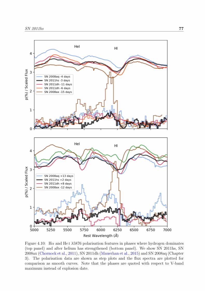
SN 2011hs 77
Figure 4.10: Hα and He i λ5876 polarisation features in phases where hydrogen dominates(top panel) and after helium has strengthened (bottom panel). We show SN 2011hs, SN2008ax (Chornock et al., 2011), SN 2011dh (Mauerhan et al., 2015) and SN 2008aq (Chapter3). The polarisation data are shown as step plots and the flux spectra are plotted forcomparison as smooth curves. Note that the phases are quoted with respect to V-bandmaximum instead of explosion date.

SN 2011hs 78
Another common feature of the SN 2011hs and SN 2011dh data is the coupling between
the P.A. of the Hα and He i polarisation and that of the continuum. Mauerhan et al. (2015)
suggested this was best explained by clumpy excitation by plumes of nickel rising from the
core. This could also be the case in SN 2011hs, and would fit in with the scenario of an
off-axis energy source described in Section 4.5.1, where 56Ni plumes rising from the core
could break the global bi-axial geometry of the outer ejecta.
The presence of an asymmetric nickel distribution have numerous explanations. In the
case of the jet powered bipolar explosion of SN 1987A, asymmetric nickel distribution was
suggested to cause polarisation (Chugai, 1992). Alternatively, 3D simulations by Wong-
wathanarat et al. (2013) showed asymmetric distributions of nickel in neutron star kick
scenarios, where the iron group elements are ejected in the direction opposite that of the
kick imparted on the remnant. These simulations, however, used progenitors of mass 15-20
M� at explosion, which is not consistent with the mass limits derived by Bufano et al.
(2014) for SN 2011hs (MZAMS= 12-15M�). This relatively low mass for the progenitor
of SN 2011hs could imply the presence of a binary companion. Indeed, SN progenitors
with MZAMS< 20 M� require binary interaction to lose enough mass to result in stripped
envelope SNe (Dessart et al., 2011). It was proposed by Hoflich (1995) for the case of
SN 1993J that an off-centre energy source could be the result of binary interaction, where
the asymmetry results from the inner region of the ejecta still being accelerated by the
gravitational potential of the binary whereas the faster outer regions are driven far from
the orbit of the system very early. Furthermore, the binary scenario could also explain the
early asphericity through binary interaction, similarly to the case of SN 2001ig (Maund
et al., 2007). Note, however, that this is a non-unique solution to our data.
Certainly one of the most commonly shared characteristics of type IIb SNe is the pres-
ence of line polarisation associated with He i λ5876 and Hα. In Figure 4.10 we place SN
2011hs in the context of other SNe at similar spectral stages (where hydrogen dominates
and where helium starts becoming prominent). We would like to emphasise that the spec-
tropolarimetric behaviour of type IIb SNe is non-uniform. Some SNe (SN 2008ax, SN
2011dh) show a strong blend of the helium and hydrogen polarisation features before he-
lium features start strengthening as the photosphere recedes through the ejecta. At later
dates, once helium lines become stronger, the Hα feature separates from the He i λ5876
and two distinct peaks are visible. In other cases, e.g. SN 2008ax and SN 2011hs, two
distinct peaks of Hα and He i λ5876 can be seen even before helium spectral features start
deepening. It is interesting that SN 2011hs and SN 2011dh behave differently in this re-
spect, despite the other commonalities in their spectropolarimetric characteristics. These

SN 2011hs 79
disparities should be reproduced by future models of the spectropolarimetry of type IIb
SNe.
The presence of loops associated with the polarisation of strong lines has also been
observed repeatedly in type IIb SNe. One of the most extreme cases was Hα in SN 2008ax
(Chornock et al. 2011 see their figures 13 and 14). In SN 2011hs, we saw loops of Hα and
He i λ5876 at early times. Hydrogen exhibited the most prominent loop at −3 days when
hydrogen was strongest in the spectrum, whereas the helium loop only arose at +2 days
and grew at +10 days as the helium lines strengthened. In SN 2011dh the best defined
hydrogen loops are also found before helium starts showing prominent features in the flux
spectrum (see figure 4 of Mauerhan et al. 2015). Contrary to SN 2011hs, however, SN
2011dh shows significant loops in He i λ5876 even at the earliest times. Another major
difference between these two objects is in their calcium loops. As we saw in Section 4.4.2,
the calcium data in SN 2011hs has a linear structure on the q − u plane around maximum
light, and only starts exhibiting a loop 10 days after V-band maximum. In contrast, SN
2011dh shows its strongest calcium loop at the earliest epoch (9 days after explosion or 11
days before V-band maximum).
These differences in the loop behaviour of type IIb SNe, and the precise origin of the
loops of Hα and He iλ5876 in SN 2011hs at the first two epochs, are difficult to understand
without modelling. Toy models have been used in the past (e.g. Maund et al. 2010, Reilly
et al. 2016), to try to reproduce line polarisation and constrain the ejecta geometry. In
an attempt to understand the early hydrogen and helium loops (and potentially extend
this to other SNe), we created a model based on the same assumptions, but used a more
methodical approach to explore parameter space (see Chapter 5). The result of this work,
however, was to demonstrate the great number of degeneracies that arise in such models,
even when considering a small number of free parameters, as well as the fact that it can
result in good fits to the data even in cases were the original assumptions are invalid. This
highlights the fact that simplified models must be considered very carefully as they may
yield misleading results.
Fully hydrodynamic simulations with radiative transfer that can simultaneously repro-
duce the flux spectrum and the corresponding polarisation features will be necessary to
better understand the varied geometry of type IIb and other core-collapse SNe. Addition-
ally, higher cadence observations, especially around and soon after maximum light, could
help better understand the variations of the ejecta geometry with depth.

SN 2011hs 80
4.6 Conclusions
We presented seven epochs of spectropolarimetry for the type IIb SN 2011hs from −3 days
to +40 days with respect to V-band maximum. The observed polarimetry data showed
very high levels of polarisation increasing towards blue wavelengths (up to ∼3 percent).
We quantified the ISP and identified that most of the observed polarisation was caused by
the interstellar component. Fits of the Serkowski law (Serkowski et al., 1975) allowed us
to constrain λmax to wavelengths < 4245A or <4700A, depending on the value of K used,
either from Serkowski et al. (1975) or Whittet et al. (1992), respectively. Such levels of ISP
have never been observed in a type IIb SN before. Similar behaviours of the interstellar
component, with low values of λmax have been seen in some type Ia SNe (Patat et al., 2015).
This may suggest enhanced levels of small silicate grains, either resulting from cloud-cloud
collisions caused by SN radiation pressure, or due to the destruction of large grains by the
radiation field (Hoang, 2017; Hoang et al., 2018). Consequently, the behaviour and level
of the ISP in the spectropolarimetric data of SN 2011hs seem to indicate the presence of
dust in the vicinity of the SN, which could reflect the mass loss history of the progenitor.
The intrinsic polarisation of SN 2011hs was retrieved after removal of the ISP com-
ponent. Significant continuum polarisation was observed at the first two epochs, with
p = 0.55 ± 0.12 percent and p = 0.75 ± 0.11 percent, respectively, corresponding to ∼10
percent departure from spherical geometry, in the context of an oblate spheroid (Hoflich,
1991). The continuum polarisation then decreased by ∼0.25 percent by +10 days and
declined further by +18 days. A strong correlation was found between the behaviour of
the P.A. of hydrogen, helium, calcium and that of the continuum, indicating they share
a common geometry. The progressive rotation of the continuum P.A. after epoch 2 can
be interpreted as the presence of an off-centre energy source being revealed. This is sup-
ported by the calcium data on the q− u plane, where a dichotomy exists between the first
two epochs at which the data form a line (indicating bi-axial geometry), and the following
epochs at which loops are observed (evidence for a departure from bi-axial geometry).
On the other hand, Hα shows the clearest loop at the first epoch when hydrogen is
strongest in the spectrum. It then diminished as He iλ5876 starts to show a loop by +3
days, which strengthens by +10 days, where helium is starting to dominate the spectrum.
These characteristics show that the lines of hydrogen and helium probe tri-axial geometries
at early times when calcium does not, and therefore line specific geometries must also be
a contributor to their polarisation. A possibility would be the presence of anisotropies in
the distribution of their line forming regions.
Compared to previously studied type IIb SNe, SN 2011hs is most similar to SN 2011dh

SN 2011hs 81
(Mauerhan et al., 2015), where a decrease in continuum polarisation over time and a cor-
relation between the P.A. of hydrogen, helium and the continuum was observed. They also
favoured an off-centre source of energy to explain their observations, namely in the form of
plumes of nickel. This could also be consistent with SN 2011hs, but is not unique and is
probably an insufficient solution to our observations.
Lastly, there are a number of features whose origins remain unknown. At +18 days
the P.A. of He iλ5876 undergoes a drastic rotation that is not coupled with that of the
continuum or other elements. Additionally, the calcium data at later dates see an increase
in polarisation and a rotation in P.A. by +60◦.
On the whole, SN 2011hs brings to the sample of type IIb SN spectropolarimetry data a
number of features that have been previously seen as well as new disparities that need to be
explained. It is clear from examples such as SN 1993J, SN 2001ig, SN 2008aq, SN 2008ax,
SN 2011dh and SN 2011hs that there is great variety in the observed spectropolarimetric
properties of type IIb SNe (Tran et al., 1997; Hoflich, 1995; Maund et al., 2007; Stevance
et al., 2016; Chornock et al., 2011; Mauerhan et al., 2015). More observations, especially
with a higher cadence around and after maximum, and detailed hydrostatic models with
radiative transfer of the current and future spectropolarimetric data, are required for us to
better understand the similarities and the diversity in the geometries of type IIb SNe.
As mentioned earlier, we will dedicate the next Chapter to reproducing a toy model
previously used in the literature, and provide a more methodical approach to determining
solutions and exploring parameter space. We will use SN 2011hs as a test case for this toy
model.

Chapter 5
A toy model to simulate supernova
polarisation
82

Toy model 83
5.1 Introduction
One of the possible ways in which line polarisation and loops can form in SNe is through
non-isotropic distributions of line forming regions – see case (ii) in Section 1.3.2. In an
attempt to better understand the ejecta geometry of the studied supernovae, we created
a Monte Carlo toy model that could in principle be used to reproduce observations and
therefore help us pin down possible ejecta geometries. Similar models have been created
in the past (e.g. Wang et al. 2007; Maund et al. 2010; Reilly et al. 2016), and this model
is most similar to that of Reilly et al. (2016), with minor differences in the physics and a
major step towards the systematic exploration and determination of the best parameters.
Firstly, the model itself and the assumptions made are described in Section 5.2, the way
we quantify goodness of fit is laid out in Section 5.3, then the sampling method used to
determine the best parameters is detailed in Section 5.4. The implementation and testing
are discussed in Section 5.5, the model is trialed using our SN 2011hs data in Section 5.6
and finally limitations are discussed in Section 5.7.
5.2 The model
The first step in the creation of the model is to simulate the radiation coming from the
photosphere (surface of last scattering) of the supernova. The photosphere is defined in two
dimensions by an ellipse with semi-major axis a and semi-minor axis b. Photon packets are
generated by randomly assigning them a position within the ellipse (hence ”Monte Carlo”).
The projected radius in 2D at a given x, y position1 is then:
r =√x2 + y2, (5.1)
and the radius of the ellipsoidal photosphere at a given x coordinate is:
R =
√x2 + b2 × a2 − x2
a2. (5.2)
Following Maund et al. (2010), it is then possible to map a linear spherical limb dark-
ening model to calculate the intensity I(r) (ranging from 0 to 1) of a packet of photons
1In Cartesian coordinates with the origin placed at the centre of the photosphere.

Toy model 84
Figure 5.1: Intensity given to individual photon packets in a photosphere modelled with105 photons, an axis ratio E = 0.86 and PTPL = 30%.
emitted at a distance r from the origin:
I(r)
I(0)= 1− k ×
(1−
√1− r2
R2
), (5.3)
where k = 0.5 (Maund et al., 2010), and I(0) is the intensity at the centre, which is set to
1. This intensity profile is illustrated in Figure 5.1.
Additionally, each photon packet is assigned a polarisation (ranging from 0◦to 180◦)
that is either randomly selected from a uniform distribution or set to be tangential to
the photosphere at the position of the packet. The probability for a photon packet to
be tangentially polarised (P>) will increase from 0 at the centre of the photosphere to a
maximum value at the limb, according to the following quadratic probability function:
P> = PTPL×(r
R
)2
(5.4)
where PTPL is the Probability of Tangential Polarisation at the Limb, which is fine tuned
for a given axis ratio E = a/b to produce a net degree of polarisation (before absorption)
that is consistent with the results of Hoflich (1991), see Section 5.5.2. A map of the
probability for a packet of photon to be polarised tangentially to the photosphere as a
function of radius is given in the top panel of Figure 5.2, for an arbitrary PTPL ∼30% and

Toy model 85
axis ratio E = 0.86. Additionally, we show in Figure 5.2 the polarisation of the photon
packets within a circular photosphere for a PTPL of 10 percent and 90 percent. This clearly
demonstrates that in practice the packets from the centre of the photosphere are indeed
randomly polarised and that a high PTPL imparts strong order to the polarisation of the
photons at the limb.
Line forming regions were assumed to have very large optical depth τ � 1 such that all
the photons behind these regions would be absorbed. Previous models by Reilly et al. (2016)
include a number of geometries for the absorbing regions: circles, ellipses, triangular lobes,
edge-on disk-like CSM. However, the solutions for these models were found through manual
trial and error and therefore did not fully explore parameter space. This is understandable
as the inclusion of complex shapes increases the number of dimensions of parameter space
(compared to e.g. a circle). For example, a singular circular absorbing region is defined by
3 parameters in 2 dimensions: the coordinates for the centre (x, y) and a radius (rabs). An
ellipse on the other hand is defined by a centre (x, y), a semi-major axis a, a semi-minor
axis b and an orientation θ, bringing the dimensionality of parameter space to 5.
One of the goals of this investigation, however, is to perform a systematic parameter
search to identify potential degeneracies. Consequently, a good starting point to this ex-
ploration is to focus on the most simple configuration: a single, circular absorption region.
In summary, each model is defined by 5 parameters, 2 of which are set by the obser-
vations and the literature (E and PTPL), and the other 3 are free parameters that define
the absorption region xfree = (x, y, rabs).

Toy model 86
Figure 5.2: Top: Probability of individual photon packets to be given a polarisation tan-gential to the photosphere. Modelled with 105 photons, an axis ratio E = 0.86 and PTPL= 30%; Bottom: Polarisation angles of 10,000 photon packets in circular photosphereswith PTPL 10 percent (left) and 90 percent (right).

Toy model 87
5.3 Quantifying the goodness of a model
After creating a model, it is important to quantify how well it reproduces the observed
data. There are 3 quantities that are taken into account when comparing a model to
observations: the net Stokes parameters q and u that result from the model, and the ratio
of the flux after and before absorption (Fline/Fcont).
The net Stokes parameters of a model are calculated by averaging the Stokes parameters
of all the photon packets, weighted by intensity. As for Fline/Fcont, it is trivial to compute
in the model by dividing the flux after absorption by the flux before absorption, but it can
be difficult to accurately estimate it from the data. As a true continuum cannot be derived
for the spectroscopic data, it is approximated as a straight line traced between 2 points on
either side of the P Cygni profile of interest. This process is done manually and visually;
an illustration of continuum determination is given in Figure 5.3.
Once the Stokes parameters and flux ratio of the model (qmodel, umodel and (Fline/Fcont)model)
and of the observed data (qobs, uobs and (Fline/Fcont)obs) have been calculated, the goodness
of the model can be quantified. This is done by simply computing the residuals between
the observed quantities and the modelled quantities. The models were considered “good”
when the results fell within 1σ of the observed data2 .
Because the parameters in xfree are correlated, providing error bars on individual pa-
rameters would not be very informative and potentially misleading. To help visualise the
results, the models found within 1σ of the observations are plotted with a colour map used
to indicate the better solutions (the lighter the colour the less deviation from observed
values). This is particularly effective at illustrating the level of degeneracy for a specific
observation/model, as can be seen in Figure 5.4
2Although see exceptions in Section 5.6
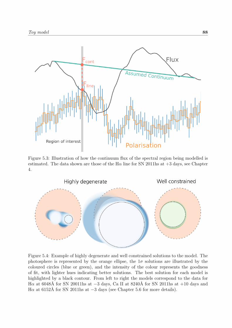
Toy model 88
Figure 5.3: Illustration of how the continuum flux of the spectral region being modelled isestimated. The data shown are those of the Hα line for SN 2011hs at +3 days, see Chapter4.
Figure 5.4: Example of highly degenerate and well constrained solutions to the model. Thephotosphere is represented by the orange ellipse, the 1σ solutions are illustrated by thecoloured circles (blue or green), and the intensity of the colour represents the goodnessof fit, with lighter hues indicating better solutions. The best solution for each model ishighlighted by a black contour. From left to right the models correspond to the data forHα at 6048A for SN 20011hs at −3 days, Ca II at 8240A for SN 2011hs at +10 days andHα at 6152A for SN 2011hs at −3 days (see Chapter 5.6 for more details).

Toy model 89
5.4 Exploring parameter space
As a first approach, the models were run with one (and only one) circular line forming
region, which is defined by the location of its centre and its radius. This is the geometry that
is defined by the smallest number of free parameters, which is why we chose it to start our
exploration of parameters space. There are only three free parameters xfree = (x, y, rabs) –
see Section 5.2.
In order to find the best solutions for xfree, parameter space needs to be explored
effectively. Firstly, it is possible to restrict the parameters that need to be investigated by
making use of the fact that Stokes parameters are quasi vectors (i.e. the 0◦and 180◦direction
are the same). This means that for each xfree, there is an equivalent set of parameters x′free
(rotated by 180◦) that returns the exact same solutions. As a result, all possible values of
y and half of the possible values of x were sampled.
We then perform a grid search and create look-up tables to summarise the output
(qmodel, umodel and (Fline/Fcont)model) for each xfree. These tables are specific to a particular
axis ratio, but can otherwise be used no matter which element or velocity slice is being
investigated. This avoids duplicating simulations.
In practice it was computationally time consuming to create look-up tables that explore
parameter space finely enough to consistently provide 1σ solutions. To address this prob-
lem, look-up tables were created for the whole of parameter space with a moderately fine
grid. Region (or regions) of parameter space that yielded good solutions for a particular
set of target values (qobs, uobs and (Fline/Fcont)obs) were then identified, and a finer grid was
produced for this particular region.
5.5 Implementation
None of the previous codes used for the toy models of Reilly et al. (2016) or Maund et al.
(2007b) were available, and I therefore had to re-create the model described in Section 5.2,
in addition to developing the parameter search code. This was done entirely in Python.
The photosphere is implemented as an object that contains information about each
individual photon packets, mainly: the Cartesian coordinates of the photon, the Stokes
parameters q and u of each photon, and their intensity. Before adding absorption regions
and trying to model some data, simple tests were performed to ensure that the integrated
polarisation of the generated photosphere was consistent with expectations.

Toy model 90
5.5.1 Testing
One of the first steps in testing this model was to ensure that the integrated polarisation
of a circular photosphere was null. In order to check this I created a large number of
photospheres (1000), with axis ratio of 1, 105 photon packets each, and a PTPL of 20
percent. Their respective q and u were calculated and used to infer the probability density
function (PDF) of the Stokes parameters. The resulting PDF for q and u is plotted on the
top panel of Figure 5.5. On average we find the Stokes parameters to be q = 0.007± 0.22
and u = 0.002 ± 0.23, where the uncertainties here are the standard deviations of the
individual Stokes parameters recorded for the 1000 photospheres.
Although these results show that when modelling a circular photosphere null polarisa-
tion is indeed retrieved, the level of uncertainty is too high for most practical uses, since the
polarisation levels are usually a few tenth of a percent. Increasing the number of iterations
does not affect these uncertainties, as they are related to the number of photon packets
being created for each photosphere. We can check this by creating 100 photospheres with
106 photon packets. The resulting PDF of the Stokes parameters is shown in the middle
panel of Figure 5.5.
In this case the average Stokes parameters are q = 0.005 ± 0.070 percent and u =
−0.004 ± 0.069 percent.The errors are reduced by a factor of 3.14 for q and 3.33 for u.
This is consistent with the expectation from Poisson statistics that the noise level should
decrease by a factor of√N given an increase of the number of photon packets by a factor
of N .
After showing that the circular photosphere case was be well-behaved, it was important
to test the polarisation resulting from the introduction of asymmetry. In order to do this, I
chose to simulate a very extreme configuration with an axis ratio of 99. In the case of this
very elongated photosphere, most of the photon packets are near the limb, and therefore
the polarisation should tend to the chosen PTPL. Additionally, the polarisation excess will
be found to be tangential to the symmetry axis, such that if the photosphere is elongated
in the 0◦direction, we should expect the polarisation to be found in the −q direction (and
null in u).
For these tests 1000 photospheres with 105 photon packets and an elongation in the
0◦direction were simulated. As before, a PTPL of 20 percent was used.
The average Stokes parameters are found to be q = −19.22± 0.24 and u = 0.009± 0.20
percent and their PDF is shown in the bottom panel of Figure 5.5. As expected, the
polarisation tends to the PTPL (20 percent) in the −q direction, and Stokes u is consistent
with zero polarisation.

Toy model 91
Figure 5.5: Probability density functions of the Stokes parameters for 1000 circular pho-tospheres with 105 photon packets (top panel); 100 circular photospheres with 106 packets(middle panel); 1000 photospheres with 99 percent asymmetry and 105 photon packets(bottom panel).

Toy model 92
Figure 5.6: Comparison of the relation between polarisation and axis ratio E for our modelusing a PTPL of 16.5 percent (orange) 30 percent (blue) and that of Hoflich (1991). Theblack line was reproduced from their Figure 4. Note that the minor peaks and troughs inour polarisation are caused by noise.
Consequently, we are confident that the model imparts polarisation as expected.
5.5.2 Fine tuning the PTPL
As mentioned in Section 5.2 the PTPL is fine tuned to a given axis ratio such that the
resulting polarisation before considering absorption regions is consistent with the results of
Hoflich (1991), see their figure 4. This step is necessary for consistency, as we derive the
axis ratios from the cross-matching of our observations to the results of Hoflich (1991).
The relation between E and p in this model and in that of Hoflich (1991) differ (see
Figure 5.6), since here we consider no physics and simply impart polarisation according to
a power-law (see Eq. 5.4). As a result, a single value of PTPL is not sufficient to reproduce
the expected photospheric polarisation for all axis ratios and fine tuning to specific values
of E is necessary.
In practice this was done by simulating 100 photospheres with 106 photon packets for
a range of PTPL of with increments of 0.5 percent. For each PTPL the average degree
of polarisation p and associated errors were calculated and compared to the continuum
polarisation measured from the data.
Toy model 93
5.5.3 Implementing absorption regions and parameter space ex-
ploration
After fine tuning the PTPL to ensure that an appropriate level of continuum polarisation
is being generated, absorption regions can be added to model line polarisation. The ab-
sorption region, since it is assumed to have very high optical depth such that all underlying
photon packets are removed from the simulation, can be implemented with a simple mask.
As previously mentioned, one of our main objectives is to systematically explore param-
eter space to find all good solutions and understand potential degeneracies. Our grid search
approach for 3 free parameters required thousands of simulated systems (photosphere +
absorption region), but due to the nature of Monte Carlo methods, photospheres simulated
with the same parameters may yield slightly different results. Additionally, re-generating
a million photon packets and their associated polarisation is computationally intensive.
Therefore, we favoured an approach where the photosphere were not re-created for every
simulation. Instead, a single instance of the photosphere object was created and its state
was saved to a file (“Pickled”). A range of absorption regions with parameters xfree could
then be modelled by calling in the object, masking the appropriate areas, and calculating
the integrated polarisation.
5.6 Application to SN 2011hs
We applied the toy model to SN 2011hs for the polarisation features of He i λ5876, Hα and
Ca ii at −3, and +2 days, where the assumption of a bi-axial ellipsoid for the geometry of
the photosphere seems robust (see Section 4.4). We also applied our models to epoch 3 (+10
days), where this assumption is not expected to be valid, for reasons that are discussed in
the next section. For these epochs the asymmetry was ∼10 percent, and the fine tuned
PTPL for an axis ratio of 0.87 was found to be 30 percent.
The number of photon packets used in each simulation was determined by the precision
required given the uncertainty on the observations that were being modelled. From Section
5.5 we know that for 106 photons the errors on q and u are ∼0.07 percent. Better precision
can be achieved with more photons (e.g. Reilly et al. 2016 used 107 photons), but the
run time scales linearly with photon number. Additionally, due to Poisson statistics, an
increase in run-time by a factor of 10 would only result in an increase in SNR by a factor of
∼√
10. Given the errors on the observational data investigated, models with 106 photons
optimised for shorter run times whilst providing sufficient precision.
The toy model solves for one wavelength bin at a time, but in an attempt to visualise

Toy model 94
the 3D structure of the line forming regions we selected 2 to 3 wavelength bins per line to
model. This is an alternative between modelling only one bin per line feature (resulting in
no depth information), and running models for all bins, which is unnecessarily laborious
as successive bins will have very similar solutions given the size of the errors on our data.
Additionally, if a polarisation feature showed two components, we made sure to select bins
sampling them both. Within those guidelines, the choice of bins is arbitrary, and other
combinations of bins could have been chosen to obtain similar results. A summary of the
target values for the bins chosen is given in Table 5.1.
In Figure 5.7, we show the models that could reproduce the observed polarisation data.
In most cases the solutions within 1 σ are shown, although some results are presented to 1.2,
1.5 and even 2 σ (as indicated by the numbers on the visual representation of the models
shown in Figure 5.7). These cases arose when parameters could not be found down to the
1-σ level, and were the result of solutions being confined to very small regions of parameter
space. Finer grids were explored, but due to time constrains we did not always reach the
1-σ level, and halted simulations when sufficient precision was obtained. As can be seen
in Figure 5.7, these cases yielded the most consistent solutions, with best constrained free
parameters. This suggests that no solution exist within 1-σ. In these particular cases we
find good agreement with the observed parameters, and the fitting issues arise in the line
to continuum flux ratio. This is most likely due to the inaccuracy of the continuum flux
estimate and the small formal errors on (Fline/Fcont)obs.
This type of visualisation, if accurate, can be complementary with Polar Plots (see
Section 4.4), as they provide a view of the distribution of line forming regions as projected
on the sky whilst polar plots show the P.A. of polarisation line features with depth.
We want to emphasise here that a model contains only one circular absorption region,
and the multiplicity observed in some cases in Figure 5.7 is just a result of the uncertainty
on the possible location of the absorption region and shows the degeneracy of the solutions.

Toy
model
95
Table 5.1: Measured values to be reproduced by the models shown in Figure 5.7.
He I 5876 Hα CaII
−3 days
5615A 5660A - 6048A 6152A 6257A 8046A 8136A 8195Aq 0.69 ±0.18 0.51 ±0.17 - 0.62 ±0.18 0.91 ±0.19 0.51 ±0.19 1.22 ±0.22 1.53 ±0.24 0.79 ±0.24u -0.051 ±0.16 -0.24 ±0.16 - -0.21 ±0.16 0.21 ±0.17 0.09 ±0.17 -0.09 ±0.20 0.27 ±0.22 -0.14 ±0.22
Fline/Fcont 0.91 ±0.02 0.886 ±0.020 - 0.948 ±0.022 0.690 ±0.018 0.592 ±0.016 0.81 ±0.20 0.604 ±0.046 0.604 ±0.007
+2 days
5571A 5675A 5705A 6137A 6271A 6316A 8061A 8165A 8240Aq 0.25 ±0.16 0.64 ±0.18 0.55 ±0.18 0.96 ±0.18 0.95 ±0.20 0.66 ±0.19 1.17 ±0.21 1.25 ±0.23 1.25 ±0.27u -0.66 ±0.15 -0.62 ±0.16 -0.77 ±0.16 -0.42 ±0.16 -0.20 ±0.18 -0.17 ±0.17 -0.63 ±0.19 -0.56 ±0.21 -0.66 ±0.26
Fline/Fcont 0.94 ±0.03 0.72 ±0.02 0.81 ±0.03 0.523 ±0.017 0.556 ±0.018 0.78 ±0.03 0.495 ±0.017 0.443 ±0.015
+10 days
- 5720A 5779A 6167A 6301A - 8240A 8315A 8374Aq - 0.12 ±0.20 0.25 ±0.19 0.55 ±0.19 0.53 ±0.21 - 0.20 ±0.3 0.45 ±0.29 -0.136 ±0.29u - -0.71 ±0.19 -0.47 ±0.17 -0.41 ±0.17 -0.38 ±0.19 - -0.92 ±0.3 -1.40 ±0.28 -1.046 ±0.27
Fline/Fcont - 0.441 ±0.013 0.630 ±0.018 0.73±0.02 0.450 ±0.014 - 0.36 ±0.01 0.324 ±0.011 0.404 ±0.014

Toy model 96
Figure 5.7: Best solutions of our toy model for He iλ5876, Hα and Ca iiλ8567 at −3, +2and +10 days. The target values and bins chosen are summarises in Table 5.1. The colourpallet represents the goodness of fit, where the lighter colours indicate the most likelysolutions. The grey ellipse shows the photosphere, onto which solutions yielding goodfits to the observed polarisation are superposed. The black circles indicate the absorptionregions giving the best fit. In most cases the solutions within 1 σ are shown, although someresults are presented to 1.2, 1.5 and even 2 σ, as indicated by the numbers on the visualrepresentation of the modelled ejecta. The coloured lines link the modelled bins to theirvisual representation. The flux spectrum (blue), and the degree of polarisation is shown(purple) are shown for comparison with the models.

Toy model 97
5.7 Degeneracies and Limitations
As can be seen in Figure 5.7, a number of cases show very high levels of degeneracy (e.g.
calcium at +10 days, helium and hydrogen at −3 days). This is a concern because our
choice of only simulating one circular absorbing region resulted in a low number of free
parameters (three), which is the simplest test case. Using more complex geometries as
done in Reilly et al. (2016), or multiple absorbing regions, would result in a greater number
of free parameters and a greater number of degeneracies. Consequently, the veracity of
similar toy models of polarisation with more complex geometries is a cause for concern,
and such results should be taken with great caution if parameter space has not been fully
explored. It should also be noted that the method employed here to explore parameter space
is not scalable to high numbers of parameters. The run-time of the current implementation,
and the need for human input to constrain parameter space before fine solutions can be
achieved, does not lend itself to a wider application.
Additionally, it is important to note that good fits were also found at +10 days, whereas
in Chapter 4 we saw a departure from axial symmetry in the photosphere at that epoch,
therefore invalidating some of the assumptions in our model. This highlights the importance
of considering the effect of the continuum on the polarisation observed in the lines before
attempting to interpret it in the context of our case (ii), since good fits may result from
the application of such models despite potential issues with the original assumptions.
On the whole, if the degeneracies of these models and the effects of the continuum
polarisation are not fully understood, the results of such simulations could lend themselves
to the over-interpretation, or an erroneous interpretation, of the origin of the polarisation
associated with strong spectral lines. More complex physical models are beyond the scope
of this study, but are needed for a more accurate interpretation of the spectropolarimetric
data of SN 2011hs and other SNe.

Chapter 6
A new analysis of SN 1993J
98

SN 1993J 99
6.1 Introduction
SN 1993J was one of the first examples of the transitional Type IIb SNe, whose spectra re-
semble those of type II SNe at early days and later transition to helium dominated spectra
like those of type Ib SNe (Swartz et al., 1993; Filippenko et al., 1993). In addition to its
peculiar spectral behaviour (at the time), SN 1993J also exhibited a double-peaked light
curve. This phenomenon was explained as being the result of a late-type supergiant progen-
itor which had lost most of its hydrogen envelope through binary interaction (Podsiadlowski
et al., 1993; Nomoto et al., 1993). A massive binary companion was later discovered by
Maund et al. (2004).
In addition to the photometric and spectroscopic studies of SN 1993J, spectropolarime-
try analysis was also performed to detect asymmetries in this SN. Observational spectropo-
larimetric analyses of SN 1993J were published by Trammell et al. (1993) and Tran et al.
(1997). However, there has been debate over the level of interstellar polarisation (ISP)
present in the data. Both studies used the assumption that the emission component of the
Hα line was completely depolarised. But this has since been shown not to be necessarily
true (e.g. Tanaka et al. 2009).
Additionally, the method used in Trammell et al. (1993) assumed that the ISP in NGC
3031 could be approximated by a Serkowski law with pmax equal to the degree of polarisation
derived for the Hα emission component and λmax = 5500A. This means that a Galactic
type ISP (with a Serkowski function and a Galactic value of λmax) was used, and this is
not necessarily a good assumption, as seen in Chapter 4.
The method used by Tran et al. (1997) was not dependent on a valid Serkowski ISP,
but required an estimate of the continuum, which the authors remarked is difficult to do
and is a large cause of uncertainty. We found continuum estimates to also be problematic
in Chapters 4 and 5.
Overall, previous ISP estimates have relied on assumptions that we now know can be
erroneous. A new investigation of the ISP of SN 1993J is therefore required, and is the aim
of this work. Using data obtained from private correspondence with H. Tran (see Section
6.2), we produced our own estimate of the ISP of SN 1993J, using a similar method to
that developed for SN 2011hs (see Chapter 4), and compared our results to expectations
and literature values (Section 6.3). The new ISP was then removed and a new intrinsic
polarisation for SN 1993J is presented and analysed in Section 6.4. We compare our results
to the literature and discuss in Section 6.5 how they affect previous conclusions. A summary
of our findings is given in Section 6.6.

SN 1993J 100
Table 6.1: Data obtained from private correspondence with H. Tran. Previously publishedin Tran et al. (1997), although the coverage for some data sets differs from the originalpublication.∗Resolution† Bin size
Date Phase Telescope Coverage (A) Pixel Size (A)April 20 +26 days 3.0m Lick 3900 - 5335 + 5865-7260 1.78*April 26 +30 days 4.0m KPNO 4000 - 7250 8†
April 30 +34 days 3.0m Lick 4600 - 7394 2.36*May 11 +45 days 3.0m Lick 4600 - 7410 2.36*May 14 +48 days 2.3m Steward 4100 - 7440 4†
6.2 Observations and data reduction
We obtained from H. Tran (through J. R. Maund) the reduced spectropolarimetric and
spectroscopic data of SN 1993J at 5 epochs (summarised in Table 6.1). These data were
first presented in Tran et al. (1997), and we refer the reader to their section 2 for the details
of the observations and data reduction. It should be noted, however, that for this work the
degree of polarisation p (percent) and its error were re-calculated (when possible) from the
errors on q and u, and p was debiased using a step function as done by Wang et al. (1997).
6.3 A new ISP
Removing the interstellar component of the polarisation is crucial to understanding the
intrinsic signal from the SN. In order to derive the interstellar polarisation, assumptions
must be made. As previously mentioned, we now know that the Hα emission component is
not necessarily completely depolarised. Instead we make the assumption that at our latest
epoch (14 May 1993 / 48 days after explosion), the polarisation observed is dominated
by the ISP rather than intrinsic SN polarisation. This is true if the electron density has
decreased sufficiently such that very little light is being polarised in the ejecta by electron
scattering. Similarly to Chapter 4, we want to fit the late time data with a straight line
to estimate a wavelength dependent ISP. As in Chapter 4, we use a sigma clipping method
since the data on 14 May 1993 have a low SNR. Additionally, the data below 4500A at
this epoch show a notable increase in noise (see Figure 6.1). Since the spectral features
of interest are located above 4500A, and given that 2 of our data sets have no data below
4600A (see Table 6.1), we choose to fit only the data with wavelength > 4500A.
A full discussion of the caveats of this method is given in Section 6.5.1, as well as a com-

SN 1993J 101
parison to historical derivations of the ISP for SN 1993J and alternative ISP determination
schemes.
The fits to the q and u data are showed in Figure 6.2. We find the following ISP-
wavelength relationships:
qISP (percent) = 1.96(±0.14)× 10−4 × λ− 0.72(±0.08) (6.1)
uISP (percent) = −0.99(±0.13)× 10−4 × λ+ 1.11(±0.08) (6.2)
where λ is in A, the gradients have units of A−1 and the intercepts are unit-less.
A comparison of the intrinsic polarisation of SN 1993J on April 30 as obtained in this
work and as estimated by Tran et al. (1997) is given in Figure 6.3. On the whole, our ISP
correction lowers the overall p levels of SN 1993J. In particular, the near zero degree of
polarisation associated with the blue parts of the spectrum (where line blanketing occurs)
and in the spectral regions associated with strong emission lines is consistent with the
expectation that these spectral regions should show little polarisation.
It is also in line with the remark of Chornock et al. (2011): when comparing their
data of SN 2008ax to other IIb SNe (including SN 1993J), they observed that the level of
polarisation on April 30 near 6600A in the Hα peak (∼0.7 percent) reported by Tran et al.
(1997) was high. They suggested that a different ISP estimate for SN 1993J could lower
the polarisation levels of SN 1993J in this spectral region, and this is seen to happen with
our ISP estimate (see Figure 6.3).
Overall, we are confident that our ISP removal method is an improvement on previous
methods and we use our estimates to correct the data we have for SN 1993J.
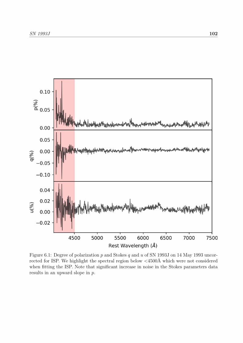
SN 1993J 102
Figure 6.1: Degree of polarization p and Stokes q and u of SN 1993J on 14 May 1993 uncor-rected for ISP. We highlight the spectral region below <4500A which were not consideredwhen fitting the ISP. Note that significant increase in noise in the Stokes parameters dataresults in an upward slope in p.

SN 1993J 103
Figure 6.2: σ-clipped Stokes parameters q and u at +48 days (dark blue) w.r.t explosion;the discarded points are shown in orange. The fits to the σ-clipped data are shown inmagenta.

SN 1993J 104
Figure 6.3: Comparison of the intrinsic degree of polarisation for SN 1993J on April 30as obtained by Tran et al. (orange) and in this work (red). The polarisation before ISPremoval is also shown in grey, as well as the scaled flux spectrum in black.
6.4 Intrinsic Polarisation
6.4.1 Degree of polarisation
In Figure 6.4 the ISP corrected degree of polarisation of SN 1993J is presented alongside
the flux spectrum from +9 days to +48 days (with respect to explosion date). At our first
epoch the data are completely dominated by noise, but the data at +30 and +34 days show
very clear line polarisation features.
+30 days
At +30 days, helium and hydrogen polarisation features are strong and complex, showing
multiple peaks. The wavelength, degree of polarisation p and P.A. of the strongest features
are summarised in Table 6.2.
The strongest peak at that epoch is that of Hβ; it is very broad, spanning ∼100A
and reaching a polarisation of level of 1.8 percent. Hα also exhibits a very broad feature,
extending from ∼5960 to 6415 A. The absorption minimum of the P Cygni profile of Hα is
correlated with a strong peak reaching a maximum polarisation of p = 1.20± 0.13 percent

SN 1993J 105
Figure 6.4: ISP corrected degree of polarisation of SN 1993J (black) and scaled fluxspectrum (red). The errors on the polarisation are shown in blue, although note that we donot have errorbar for the last epoch. The grey shaded areas show the telluric line regions.

SN 1993J 106
Table 6.2: Summary of the main polarisation peaks in the data of SN 1993J. The bin sizecan be found in Table 6.1.
Element Wavelength / Velocity p P.A(A/ km s−1) (percent) (◦)
April 26: +30 days
Hβ 4720 / −8,800 km s−1 1.8±0.3 18±6HV He i λ5876 5632 / −12,500 km s−1 0.93±0.11 43.0±0.3
He i λ5876 5728 / −7,550 km s−1 1.02±0.08 46.3±0.2HV Hα 5912 / −30,000 km s−1 0.60±0.12 23±5HV Hα 6040 / −24,000 km s−1 0.91±0.12 32± 2HV Hα 6072 / −22,500 km s−1 0.94±0.11 37±1HV Hα 6152 / −18,800 km s−1 0.90±0.11 43.4±0.2
Hα 6304/ −11,800 km s−1 1.20±0.13 45.9±0.1HV He i λ6678 6456/ −10,000 km s−1 0.40±0.13 115±7
He i λ6678 6600/ −3,500 km s−1 0.63±0.07 88±74He i λ7065 6952/ −4,800 km s−1 0.98±0.11 47±0.2
April 30: +34 days
Hβ 4695-4740 / −10, 500 to −7, 500 km s−1 0.90±0.08 24◦±2HV He i λ5876 5590-5620 / −14, 600 to −13, 200 km s−1 0.78±0.05 34◦±1
He i λ5876 5715-5740 / −8, 200 to −7, 000 km s−1 1.20±0.08 32◦±1Hα 6332 / −10, 550 km s−1 1.17±0.23 36◦±2

SN 1993J 107
at 6304A. Three other distinct peaks are superposed onto the broad hydrogen feature at
6040, 6072, and 6152A, all with p∼0.9 percent. They are coincident with dips in the blue
shoulder of the Hα absorption line profile, and I interpret these as high velocity (HV)
components of hydrogen overlapping the main P Cygni profile and its associated inverse
P Cygni in the spectropolarimetry. Additionally, a very sharp peak can be observed at
5912A, offset in the blue compared to the main Hα features. This could be the result of
an even higher velocity component of hydrogen (∼30,000 km s−1).
He i λ5876 also shows a complex multi-peaked feature at +30 days. The two main
components are found at 5632 and 5728A reaching a similar degree of polarisation, p ∼1
percent (see Table 6.2 for more detail). The 5632A peak coincides with the bottom of
the absorption component of He i λ5876, whereas the other peak is associated with a blue
shoulder in the profile of the absorption component of the P Cygni profile. As a result
we refer to this second peak as a HV component of the He i λ5876 polarisation. Weaker
features (p∼0.5 percent) are found both on the blue and red side of those peaks, suggesting
asymmetries at a wide range of depth in the ejecta.
Additionally, the spectral region associated with the Hα emission, although it is mostly
depolarised, shows two peaks that are likely associated with He i λ6678 (Table 6.2), which
is seen to start developing in the flux spectrum at this epoch. Moreover, a polarisation
peak is associated with the onset of the He i λ7065 in the flux spectrum (see Table 6.2 and
Figure 6.4).
On the whole, the polarisation at +30 days is dominated by complex hydrogen and
helium features.
+34 days
The data at +34 days suffer from more noise than those at +30 days. This is due to a
combination of effects: the supernova was fading, the telescope was smaller, as are the
bins. Nonetheless, very clear peaks similar to that observed at +30 days can be seen in
the spectropolarimetric data at this epoch. For all features, excluding Hα, the degree of
polarisation and P.A. are calculated from the weighted average of the normalised Stokes
parameters in the corresponding range indicated in Table 6.2. The errors are propagated
from the errors on the weighted mean of the Stokes parameters.
At this epoch, hydrogen still exhibits a strong Hβ peak and a broad Hα feature topped
by a peak associated with the main absorption line. The Hα feature actually seems to
extend further in the blue than it did at +30 days: down to ∼5910 A.
The He i λ5876 still shows two main peaks with degree of polarisation similar to that

SN 1993J 108
observed at +30 days (see Table 6.2): one associated with the absorption minimum in
the flux spectrum, and the other associated with a blue shoulder in the profile of the
absorption line, which is interpreted as a HV component. Once again the depolarised
region corresponding to the Hα emission line is topped by a peak of He i λ6678, ∼6600A.
Additionally, the broad polarisation feature extending from 6715A to 7000A could be a
signature of He i λ7065.
All together, the polarisation data at +34 days still show very strong hydrogen and
helium features.
Late times
At +45 days and +48 days, the main He i λ5876 and Hα peak remain visible but the noise
and errorbars are such that we will refrain from making quantitative estimates of the level
of polarisation for these lines. The decrease in signal to noise ratio is caused by the fading
of the supernova, as well as the smaller telescope aperture in the case of the +48 days data.
Overall, the polarised signal at these epochs does seem lower, which would most likely due
to the decrease in electron density in the ejecta.
6.4.2 Stokes q − u plane
The behaviour of spectropolarimetric data on the q − u plots can reveal both large-scale
and small-scale asymmetries (see Wang & Wheeler 2008 for a review). When plotting the
whole data, an alignment on the q− u plane ordered with wavelength (dominant axis) can
be interpreted as the of result bi-axial geometry, from an oblate photosphere or from an
off-centre energy source in a spherical envelope – see case (i) and case (iii) in Section 1.3.2.
Additionally, changes in polarisation angle across the wavelength range of specific spectral
lines (loops), is a sign of departure from axial symmetry.
In Figure 6.5 we present the ISP corrected data of SN 1993J from +24 days to +48
days. At the first epoch, we can see some alignment in the data, but due to the level of
noise at this time caution is required. At +30 days and +34 days, some alignment may also
be present. Note that the blue points deviating from the main locus of the data at +30
days belong to the Hβ line, which is discussed below. At +45 days and +48 days the data
seem to form a circular cloud centred on the zero point, indicating no bi-axial geometry
and no significant continuum polarisation.
To check for the presence of a dominant axis we perform ODR fits on all of our data sets.
In the present data, ODR was not able to find suitable solutions for most epochs, apart
from the polarisation at +30 days, with the best fit found at angle of 101◦±2◦. Note that

SN 1993J 109
this fit did not include the bluer data points corresponding to Hβ. Although the regression
did not converge at + 34 days, the dominant axis found at +30 days seems to be a good
fit to +34 days. It is possible that the size of the errors caused the fitting algorithm not
to converge, and that binning the data at +34 days could have helped identify a dominant
axis. Unfortunately we are unable to rebin the data we were provided, since we do not
have the original flux data. Binning should be applied on the flux before we apply the
transformations described in Section 2.3.2 to find the Stokes parameters.

SN
1993J110
Figure 6.5: ISP corrected polarisation of SN 1993J on the q − u plane for April 20 to May 14 from a starting wavelength of4500A. The colorbar shows wavelength. The black line shows the dominant axis obtained when fitting the data at +30 daysand excluding the Hβ feature.

SN 1993J 111
In Figures 6.6, 6.7 and 6.8 we present the Hα, Hβ and He i λ5876 data on q−u plots. We
only show the +30 days and + 34 days data since no statistically significant line features
were observed at other epochs (see Figure 6.4).
The data corresponding to the main Hα peak show both at +30 and +34 days a linear
configuration on the q − u plane. This is indicative that this line forming region probes
a bi-axial ejecta configuration. The putative HV features of Hα, on the other hand, show
clear rotations in P.A. at +30 and +34 days. Whether these wavelengths do correspond to
HV hydrogen or not, they probe significant deviations from bi-axial symmetry.
In Section 6.4.1, we saw that the strongest polarisation features at +30 days was that
of Hβ. The Hβ data at this epoch also shows one of the most complex loop in this
thesis, exhibiting a mixture of successive anti-clockwise and clockwise rotation. Significant
departures from a bi-axial geometry are therefore evidenced by this loop. At +34 days
the error bars are larger, as is the noise. There may be some rotation of the P.A. and
departures from bi-axial symmetry, but the case is not as clear as for that of Hβ at +30
days.
The He i λ5876 line at +30 and +34 days was associated with two main polarisation
peaks, the first corresponding to the absorption flux minimum and the second interpreted
as a HV component, associated with a blue shoulder in the helium line profile (see Section
6.4.1). Both at +30 and +34 days, the main helium features show clear anti-clockwise
loops on the q − u plane. The loop at +34 days is more developed than 4 days prior,
showing 180◦rotation across the feature and a greater amplitude. Consequently, the main
He i λ5876 peak probes departures from bi-axial geometry. The high velocity components,
on the other hand a both epochs show very little P.A. rotation if any. Departures from
axial symmetry are therefore less prominent, if at all present, than in the deeper layers of
this line forming region.
Possible implications for these observation are discussed in Section 6.5.2.

SN 1993J 112
Figure 6.6: ISP corrected Hα polarisation of SN 1993J on April 26 (+30 days) and April30 (+34 days). The colorbar shows velocity. The inset plots show the flux spectrum indark grey and the polarisation in light grey except for the data points shown on the q − uplots, which are shown in with the corresponding colormap.
Figure 6.7: ISP corrected He i Hβ polarisation of SN 1993J on April 26 (+9 days) andApril 30 (+13 days). The colorbar shows velocity. The inset plots show the flux spectrumin dark grey and the polarisation in light grey except for the data points shown on theq − u plots, which are shown in with the corresponding colormap.

SN 1993J 113
Figure 6.8: ISP corrected He i λ5876 polarisation of SN 1993J on April 26 (+9 days) andApril 30 (+13 days). The colorbar shows velocity. The inset plots show the flux spectrumin dark grey and the polarisation in light grey except for the data points shown on theq − u plots, which are shown in with the corresponding colormap.
SN 1993J 114
6.5 Discussion
6.5.1 Assumptions in ISP estimates and alternative methods
In Section 6.3 we presented a new method to estimate the ISP in the data of SN 1993J. It
differs from previous methods employed by Trammell et al. (1993) and Tran et al. (1997)
in a number of ways. Firstly, the historical analyses used the assumption that Hα emission
was completely depolarised. This idea stems from the fact that the emission component of
P Cygni profiles are the result of light being scattered into the observers line of sight by
resonant scattering, which is a depolarising process. However, the superposition of an He i
λ6678 absorption component and its associated polarisation can render the assumption
of complete depolarisation in this region of the spectrum invalid. To derive their ISP,
Trammell et al. (1993) and Tran et al. (1997) used the data on April 20 (+26 days) and
justified their assumption by saying that no helium component could be seen. However,
the flat top profile of Hα on April 20 (see Figure 6.4) suggests that some He i λ6678 is
present, putting the assumption of complete depolarisation into question.
In order to compute our ISP, we assumed that the data at our latest epoch was represen-
tative of the ISP. This is valid if the electron density in the ejecta has decreased sufficiently
such that intrinsic supernova polarisation is negligible. This assumption, however, is not
completely exact, as line polarisation features remain somewhat visible at +48 days. Con-
sequently, some latent SN continuum polarisation may have biased our ISP estimate.
Another difference between our ISP and previous estimates is the wavelength depen-
dence. In Trammell et al. (1993), a Serkowski type law was used, whereas in Tran et al.
(1997) negligible wavelength dependence was assumed. In the former case, this poses the
question of the validity of the Serkowski law (Serkowski, 1973) to account for the dust
properties in other galaxies and in the vicinity of SNe. We now know of a number of cases
where the form of the ISP in the line of sight to the SN have been shown to be significantly
different from that of the Milky Way (e.g.Patat et al. 2015, Chapter 4), and therefore this
assumption should be used with care. Using the approximation of a constant ISP can be
sufficient if the wavelength dependency is very shallow and consequently negligible given
the noise levels.
The ISP Stokes parameters we derive in Section 6.3 do not make use of the Serkowski
assumption, and are expressed as linear functions of wavelength (see Eqs 6.1 and 6.2).
This also results in a wavelength dependence in the P.A. of the ISP. This can be caused
by the superposition in the line of sight of dust clouds with different particle sizes and
orientations, or by the superposition of ISP and some latent intrinsic SN polarisation, as

SN 1993J 115
mentioned above (Coyne & Gehrels, 1966).
Despite the caveats associated with our assumptions, the ISP estimates we derived
result in ISP removed data (see Figure 6.4) which show a behaviour that is consistent with
expectations. As mentioned in Section 6.3, the blue region of the spectrum between 4600
and ∼5500A is mostly depolarised, apart from some peaks of line polarisation. This is
consistent with the expected depolarisation in that part of the spectrum caused by line
blanketing (Howell et al., 2001). Moreover, Hα emission is associated with polarisation
that is close to zero, apart from peaks associated with the absorption component of He i
λ6678. Finally, our new ISP solves the issue of the high level of polarisation (∼0.7 percent)
observed near 6600A in the Tran et al. (1997) data on April 30, which was highlighted by
Chornock et al. (2011) and which they suggested could be solved if different ISP values
were to be used.
As a result we are confident that the method described in Section 6.3 was successful
in estimating the ISP present in the SN 1993J data. Nevertheless, this method should be
applied with care and with full consideration of the caveats mentioned above, particularly
when fitting data that show residual intrinsic SN polarisation.
An alternative way to estimate the ISP is to make use of the assumption that the blue
part of the spectrum is completely depolarised due to line blanketing (Howell et al., 2001),
and simply average the Stokes parameters in this range. To test this method we applied
it to April 20, 26, 30 and May 11. A weighted average of the Stokes parameters was
performed; the errors on the weighted mean were also calculated, and propagated through
to the degree of polarisation and polarisation angle. The degree of polarisation was also
debiased. The wavelength ranges used and resulting ISP values are given in Table 6.3
alongside the literature ISP values and equivalent 5200A ISP values obtained from Eqs 6.1
and 6.2, for comparison purposes. Note that the range used for the average on April 20 is
different from the other epochs because no data is available between 5300A and 5500A.
On the whole, the estimates in Stokes parameters, degree of polarisation and polari-
sation angle using this method vary from epoch to epoch. This is inconsistent with the
behaviour of the ISP, which is constant on short timescales, and shows that the results
were biased by intrinsic polarisation. It is interesting to note that the values obtained from
May 11 (+48 days) are very close to the ISP values we derived at 5200A. This can be
understood as the result of a decreasing amount of intrinsic polarisation at later dates due
to the decreasing electron density, causing the observed polarisation to be dominated by
ISP.
The main issue with this method is that, although depolarisation of the continuum

SN 1993J 116
Table 6.3: Comparison of ISP values obtained using different methods.
Date Wavelength q u p P.A.Assuming depolarisation in the blue
April 20 4500-5300A 0.58±0.03 0.19±0.03 0.61±0.03 9◦±5◦
April 26 4800-5500A 0.61±0.05 0.65±0.04 0.89±0.04 23◦±1◦
April 30 4800-5500A 0.42±0.03 0.53±0.03 0.68±0.02 26◦±1◦
May 11 4800-5500A 0.28±0.04 0.45±0.04 0.53±0.04 29◦±1◦
sigma clipping methodMay 14 5200A 0.30±0.15 0.60±0.15 0.63±0.15 32◦±3◦
Tran et al.April 20 6390-6890 0.60 -0.19 0.63 171◦
Trammell et al.April 20 Hα emission 0.55 -0.95 1.1±0.1 150◦±0.1◦
through line blanketing is a real effect, this region of the spectrum does sometime show
significant line polarisation, as can be clearly seen in SN 1993J at +30 days, or in SN
2008aq at +27 days (see Chapter 3). Consequently, although keeping in mind the expected
effects of line blanketing makes for a good sanity check, it is difficult in practice to use it
to find reliable ISP values.
6.5.2 Interpretation of the data and comparison to previous stud-
ies
Previous studies of the spectropolarimetric properties of SN 1993J were performed by Tram-
mell et al. (1993) and Tran et al. (1997). These analyses were done at a time where intrinsic
polarisation had only been observed in one supernova – SN 1987A – and therefore mostly
focus on whether intrinsic polarisation was present in the supernova and on quantifying
the degree of continuum polarisation. In order to do this, Trammell et al. (1993) and Tran
et al. (1997) use the same method of averaging the data across a large range of wavelengths.
In the former case, they use the range 4900-6800A and find p = 1.6 percent (ISP removed)
on April 20, whereas in the latter they average their data over 4800-6800A and find p∼1
percent on April 26.
Since this wavelength range encompasses both the He i λ5876 and Hα lines, this method
will capture the presence of intrinsic polarisation, however it is not suitable to isolate the
continuum polarisation from the line polarisation. In order to estimate the continuum
independently, it is necessary to identify a region of the spectrum that is devoid of strong
lines. A good spectral range for this purpose would be between the 7630A telluric lines and

SN 1993J 117
the onset of the calcium infra red triplet absorption component (e.g. Chapter 3). However,
this region of the spectrum is not accessible in these data sets (see Figure 6.4 in Section
6.4.1), and we therefore did not attempt to calculate a continuum polarisation.
Information about the geometry of the ejecta can be inferred from the q − u plots pre-
sented in Section 6.4.2. The data as a whole showed marginal elongation on the q − u
planes (see Figure 6.5) at the first 3 epochs, indicating some degree of axial symmetry
in the ejecta. The Hα data at +30 and +34 days between about −14,000 km s−1and
−6,000 km s−1showed linear configurations consistent with bi-axial geometries. If the fea-
tures interpret as HV Hα are indeed hydrogen features, then the P.A. variation they show
on the q − u plane > −18,000 km s−1indicate a departure from axial symmetry at higher
depths. This could either be a line specific effect or the result of the global geometry. Since
no other lines probe such high velocities, it is not possible to distinguish between these two
possibilities at the present time.
Although the main peak of Hα at +30 days behaves as expected in the case of a bi-axial
geometry, Hβ shows a very complex loop –and so a complex geometry that significantly
departs from axial symmetry– at similar velocities, see Figure 6.7. Therefore, the main
feature of Hα probes a different geometry from that of Hβ at the same depth. This means
that global geometry effects are not the only source of polarisation, and some line specific
geometries must come into play.
In the case of He i λ5876, loops are seen at a depth below −9,000 km s−1at +30 and
+34 days, which contrasts with the linear configuration followed by the Hα data at similar
depths. In addition, the helium loop strengthens between +30 and +34 days, as the helium
lines in the spectrum become more prominent. Consequently, these polarisation features
seem to probe line specific geometries and departures from the global geometry.
On the whole, SN 1993J does appear to have some degree of global bi-axial geometry,
and considerable line specific departures from this axial symmetry. The bi-axial geometry
could be the result of an off-centre energy source as suggested in Hoflich (1995). Inhomo-
geneities in the distribution of hydrogen and helium could result in uneven obscuration of
the underlying photosphere, causing the observed departures from axial symmetry.
In order to better understand the geometry of the ejecta of SN 1993J, careful modelling
will be required, but this is beyond the scope of this Thesis.

SN 1993J 118
6.6 Conclusion
In this Chapter we presented a preliminary re-analysis of spectropolarimetric data of SN
1993J from +24 to +48 days with respect to explosion date obtained from private corre-
spondence with H Tran (through J. R. Maund). We estimated the ISP using a method
independent of those used by Trammell et al. (1993) and Tran et al. (1997) and found our
values to be inconsistent with the literature. Because these studies used assumptions that
we now know are not necessarily true, and since we find our ISP answering some issues
raised by Chornock et al. (2011) concerning the intrinsic polarisation of SN 1993J, we are
confident that our estimates are improvements on literature values.
In the ISP removed data at +30 and +34 days we found significant line polarisation
features of hydrogen and helium with degree of polarisation ∼1 percent in Hα and He i
λ5876. At +30 days, Hβ showed a degree of polarisation as high as 1.8 percent. Possible
HV features of Hα and He i λ5876 were also identified although spectral synthesis has not
yet been performed to confirm or disprove this.
The q−u plots of SN 1993J revealed marginal bi-axial geometry at +30 and +34 days.
Loops were seen in Hα, Hβ and He i λ5876 at different depths. The non-homogeneous
behaviour of the loops from line to line suggests that line-specific geometries are the cause
for departures from bi-axial geometry. More analysis and modelling are needed to fully
explore the new intrinsic polarisation of SN 1993J presented here.
In the following chapter we will move away from the Type IIb SNe, and present the
best spectropolarimetric data set obtained for a Type Ic-bl (to this day).

Chapter 7
A choked jet in Type Ic-bl
SN 2014ad?
119

SN 2014ad 120
7.1 Introduction
As mentioned in Section 1.2.1, broad-lined type Ic SNe (SNe Ic-bl) show extremely broad
and blended spectral features compared to “normal” type Ic SNe (e.g. SN 1997X, see
Munari et al. 1998; SN 1997ef, see Iwamoto et al. 2000; or SN 2002ap, see Mazzali et al.
2002), as a result of significantly greater ejecta velocities. A study of 17 type Ic SNe and
21 SNe Ic-bl conducted by Modjaz et al. (2016) has shown that the mean peak expansion
velocity is ∼10,000 km s−1faster in Ic-bl than in type Ic SNe over all epochs.
SNe Ic-bl have been of particular interest over the past two decades, owing to their
relation to long Gamma-Ray Bursts (GRBs) and X-Ray Flashes (XRFs) – see Section 1.2.1.
Not all SNe Ic-bl are part of a SN/GRB pair, however, which, as stated by Soderberg et al.
(2006), cannot be explained solely through viewing angle effects. This implies that the
progenitors and/or explosion mechanisms giving rise to GRB/SNe and GRB-less SNe Ic-bl
are distinct in some way.
The main model proposed to produce GRBs is the Collapsar model, whereby the rapidly
rotation core of the massive star collapses to a black hole and forms an accretion disk which
collimates jets. It has also been suggested that type Ic-bl SNe without GRBs could also
be powered by jets that have not broken out of the envelope, potentially due to shorter
central engine lifetimes (see Section 1.2.3).
SN 2014ad is a type Ic-bl SN without a detected GRB. In this Chapter we use spec-
tropolarimetry to infer geometrical properties of its ejecta and relate them to potential
explosion mechanisms. We present the best spectropolarimetric data set obtained yet for a
SN Ic-bl, extending over 7 epochs, and ranging from −2 days to +66 days with respect to
V-band maximum. We also report 8 epochs of spectroscopy ranging from −2 days to +107
days. Note that this Chapter is an update on our publication of the SN 2014ad spectropo-
larimetric data in Stevance et al. (2017). The main difference is in the size of the error
bars, as we realised after publication that the error treatment in the IRAF utilities we used
was incorrect, and caused a significant over-estimate of the uncertainties. We are pleased
to report that the conclusions drawn in Stevance et al. (2017) are completely unaffected.
In Section 7.2 we give an account of our observations and data reduction; in Section 7.3
we present our spectroscopic and spectropolarimetric results and in Section 7.4 we discuss
interstellar polarisation and analyse the intrinsic polarisation of SN 2014ad using q − u
plots and synthetic V-band polarimetry. Our results and analysis are then discussed in
Section 7.5 and conclusions are given in Section 7.6.

SN 2014ad 121
7.2 Discovery and Observations
SN 2014ad was discovered by Howerton et al. (2014) on 12.4 March 2014 in public images
from the Catalina Sky Survey (CSS, Djorgovski et al. 2011) at RA = 11:57:44.44 and δ
= -10:10:15.7. It is located in MRK 1309 (see Figure 7.1), with a recessional velocity of
1716 km s−1(Wong et al., 2006). Spectropolarimetric observations of SN 2014ad were con-
ducted with FORS2 (see Section 2.1.2) under the program ID: 093.D-0820 (PI: J. Maund).
The order sorting filter GG435 was used, which made all wavelengths below 4450 A inac-
cessible to us. Linear spectropolarimetric data of SN 2014ad were obtained at 7 epochs
between 22 March 2014 and 29 May 2014. Circular spectropolarimetric data were also
acquired on 29 March 2014 and 11 April 2014. Additionally, spectroscopic data were taken
on July 2014; a summary of observations is given in Table 7.1.
All the observations were taken using the 300V grism, providing a spectral resolution
of 12 A (as determined from arc lamp calibration frames). The spectropolarimetric data
were reduced according to the prescriptions described in Chapter 2. In order to increase
the level of signal-to-noise the spectropolarimetric data were re-binned to 45 A, which did
not affect the resolution considering the breadth of the spectral features.
1Flux Standard
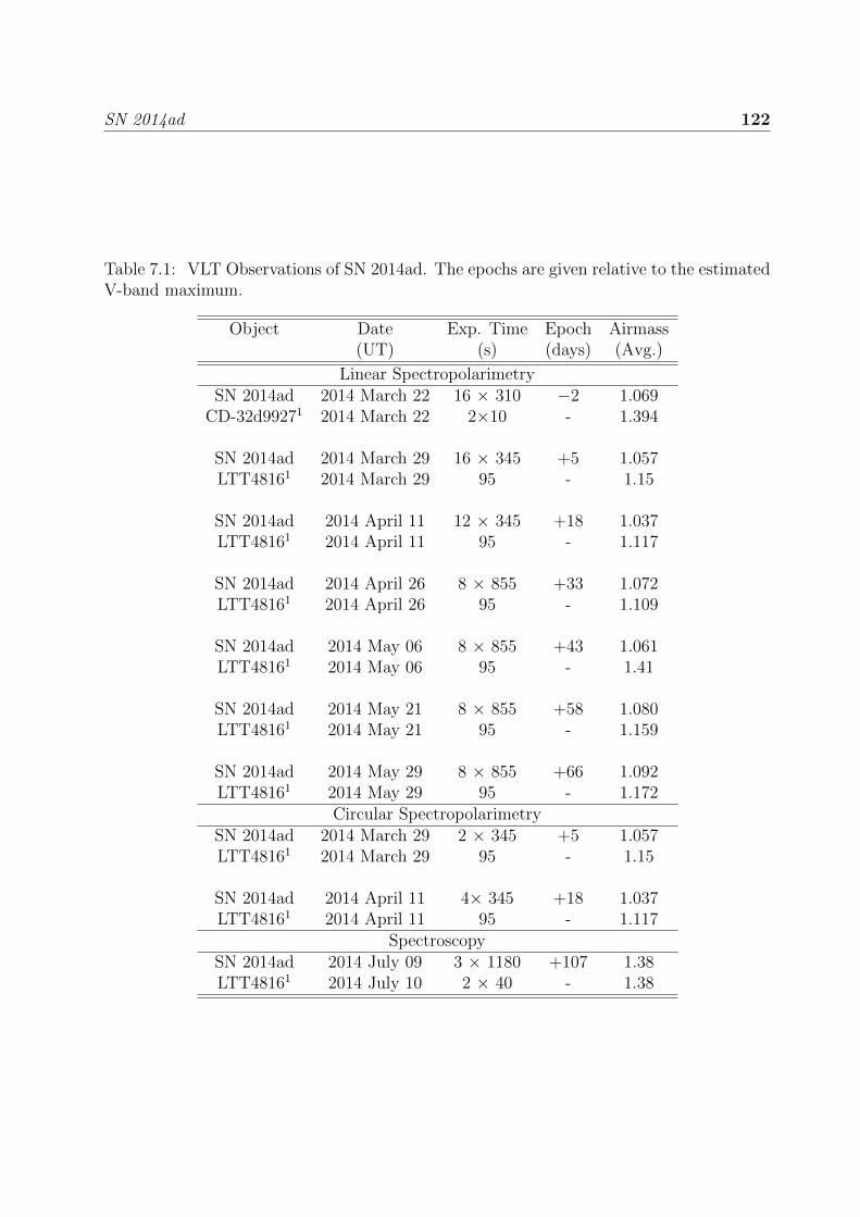
SN 2014ad 122
Table 7.1: VLT Observations of SN 2014ad. The epochs are given relative to the estimatedV-band maximum.
Object Date Exp. Time Epoch Airmass(UT) (s) (days) (Avg.)
Linear SpectropolarimetrySN 2014ad 2014 March 22 16 × 310 −2 1.069
CD-32d99271 2014 March 22 2×10 - 1.394
SN 2014ad 2014 March 29 16 × 345 +5 1.057LTT48161 2014 March 29 95 - 1.15
SN 2014ad 2014 April 11 12 × 345 +18 1.037LTT48161 2014 April 11 95 - 1.117
SN 2014ad 2014 April 26 8 × 855 +33 1.072LTT48161 2014 April 26 95 - 1.109
SN 2014ad 2014 May 06 8 × 855 +43 1.061LTT48161 2014 May 06 95 - 1.41
SN 2014ad 2014 May 21 8 × 855 +58 1.080LTT48161 2014 May 21 95 - 1.159
SN 2014ad 2014 May 29 8 × 855 +66 1.092LTT48161 2014 May 29 95 - 1.172
Circular SpectropolarimetrySN 2014ad 2014 March 29 2 × 345 +5 1.057LTT48161 2014 March 29 95 - 1.15
SN 2014ad 2014 April 11 4× 345 +18 1.037LTT48161 2014 April 11 95 - 1.117
SpectroscopySN 2014ad 2014 July 09 3 × 1180 +107 1.38LTT48161 2014 July 10 2 × 40 - 1.38

SN
2014ad123
Figure 7.1: Images of MRK 1309 with (left panel) and without (right panel) SN 2014ad. The image on the right hand sideis a SERC image from 03 August 1989 retrieved via Aladin. The image of SN 2014ad in MRK 1309 on the left-hand sidewas obtained by Stan Howerton from eleven unfiltered 20 second exposures acquired on 3.1 May 2014 using a Celestron11-inch CST and a Orion StarShoot Deep Space Monochrome Imager III. The red line superposed onto the SERC image isthe direction of the interstellar polarisation (ISP) determined for MRK 1309 (see section 7.4.1).

SN 2014ad 124
7.3 Results
7.3.1 Lightcurve
V-band observations were acquired between 12 March 2014 and 28 May 2014 (for details
see Howerton 2017). A luminosity distance of 24.7 Mpc was calculated from the redshift
of MRK1309 (z=0.005723, Wong et al. 2006), and we estimated that SN 2014ad reached
maximum with an absolute V-band magnitude of −18.8 ± 0.2 mag on 24 March 2014
(considering an extinction AV = 0.51 based on the redenning quoted in Section 7.4.1 and a
value of R = 3.1). All epochs subsequently mentioned in this paper are quoted with respect
to this date. The absolute V-band magnitude was corrected for extinction using the Milky
Way and host galaxy reddening we calculated (see section 7.4.1). An exhaustive analysis
of the lightcurve is not the main focus of this work, and we refer the reader to Sahu et al.
(2018), who have now published exhaustive optical photometry and spectroscopy of SN
2014ad. It is worth noting that they found an absolute V-band magnitude and maximum
date that were consistent with what is presented here and in Stevance et al. (2017).
7.3.2 Flux Spectroscopy
The spectral features of SN 2014ad are very broad, particularly at early times, which is
characteristic of SNe Ic-bl (see Figure 7.3). At 5 days after V-band maximum, SN 2014ad
shows broader features than SN 2002ap at +3 days, that are nearly as broad as SN 1998bw
at +4 days. Although the spectral lines become less broad as time passes, SN 2014ad
still shows features that are much broader than that of SN 1997ef 43 days after V-band
maximum. Additionally, at +33d and +43d SN 2014ad is very similar to SN 1998bw at
+38d.
In CCSNe, the line centre velocity of the Fe ii λ5169 absorption component is commonly
used as a proxy for the photospheric velocity (e.g. Modjaz et al. 2016). The extreme
line blending occurring in the spectra of SN 2014ad, however, made using this feature
unreliable (Liu et al., 2016). Consequently, we used syn++ (Thomas et al., 2011) to fit
the Fe ii blend in our spectra of SN 2014ad and determine the photospheric velocity, as well
as confirm line identification. syn++ is a radiative transfer code that assumes spherical
symmetry and no electron scattering. It allows the user to choose the ions to be added to
the synthetic spectra, and change parameters such as the photospheric velocity, the opacity,
the temperature and the velocity of each ion, in order to construct the best fit to the data.
4https://gelato.tng.iac.es/

SN 2014ad 125
Figure 7.2: De-reddened lightcurve of SN 2014ad from 12 March 2014 to 28 May 2014, usingAv = 0.51 mag and a distance modulus = 31.96 mag. Details of photometric acquisitioncan be found in Howerton (2017).
We found a photospheric velocity as high as 30,000 ± 5,000 km s−1at −2 days, decreasing
to 10,000 ± 2,000 km s−1by +66 days (see Figure 7.4). The photospheric velocities later
reported by Sahu et al. (2018) were consistent with our estimates, see their figure 10.
The extreme line blending caused by the high ejecta velocities also made line identi-
fication challenging. At all epochs, best syn++ fits were obtained for synthetic spectra
containing Fe ii, Na i, Si ii, O i and Ca ii. It was not possible to obtain uniformly good fits,
especially at later epochs due to the appearance of forbidden lines of Mg i], [O i] and [Ca ii].
We were however able to find good fits of the Fe ii complex at all epochs; Figure 7.5 shows
our fit to the spectrum of SN 2014ad at +5 days.
At the earlier epochs, the spectrum is dominated by a blend of iron lines in the region
4500-5500 A, and a deep absorption component with a minimum at ∼7500 A corresponding
to a blend of O i λ7774 and Ca ii infrared (IR) triplet. In the first epoch the emission
component of the Ca ii+ O i blend is flat topped, but it becomes prominent by +5 days.
At this epoch, a strong Si ii λ6355 emission has also emerged. Over time, line blending
diminishes as opacity decreases and we are probing the deeper, slower ejecta, however the
O i λ7774 never completely separates from the Ca II IR triplet as it does in SN 1997ef. At
later epochs, the strength of the iron blend progressively decreases, and the Ca ii IR triplet
emission strengthens. By 43 days after maximum, we can see the spectrum of SN 2014ad
starting to transition from the photospheric phase towards the nebular phase: The [O i]
emission at ∼6300 A dominates over the Si ii λ6355 emission observed at previous epochs,
and the absorption of the Ca ii IR triplet becomes increasingly flat-bottomed as the P-

SN 2014ad 126
Figure 7.3: Flux spectrum of SN 2014ad at 8 epochs (brown) corrected for recessional ve-locity. We compare with the flux spectra of the three SNe Ic-bl which most closely matchedSN 2014ad according to Gelato4: SN 1997ef (43 days after V-band maximum), SN 1998bw(at +4 days and +38 days), as well as SN 2002ap (3 days post V-band maximum). The greybands highlight telluric features. SN 1998bw is known for its connection to GRB 980425(Woosley et al., 1999), SN 1997ef was thought to be the optical counterpart of GRB 971115,but the significance of their correlation is much lower than for SN 1998bw/GRB 980425(Iwamoto et al., 2000). The narrow lines in the spectra of SN 2014ad are associated withthe interstellar medium of the host galaxy.

SN 2014ad 127
Figure 7.4: Time evolution of the photospheric velocity of SN 2014ad, as measured byfitting the spectra using SYN++
Figure 7.5: Spectrum of SN 2014ad at 5 days after V-band maximum (solid black) andmodel obtained using syn++ (dashed red). The model includes Fe ii, Na i, Si ii, O i andCa ii.

SN 2014ad 128
Cygni profile fades and is replaced by just an emission feature. At +107 days, SN 2014ad
has a typical nebular spectrum, with (semi-)forbidden lines of Mg I] λ4571, [O I] λ6300 and
[Ca II] λλ7291,7824.
7.3.3 Linear Spectropolarimetry
The degree of polarisation p and flux for each of our 7 epochs of linear spectropolarimetry
are shown in Figure 7.6. At −2 days, 5 peaks can be seen in the polarisation spectra at
∼5672A (p = 1.10 ± 0.03 percent), 6030A (p = 1.10 ± 0.02 percent – averaged between
5985A and 6075A), 6880A (p = 1.60± 0.03 percent), 7685A (p = 1.30± 0.05 percent), and
8130A (p = 0.83± 0.03 percent – averaged between 8093A and 8181A).
The 6880A peak shows the highest level of polarisation recorded in our data set. This
feature is likely the result of O i λ 7774 at −34,500 km s−1. As for the other features, the
5672A peak in polarisation is associated with Si ii λ6355 with velocity −32,200 km s−1, the
7685 A feature arises from Ca ii at −30,900 km s−1, and the peak seen at 8130A could be
O i λ9264 at −36,600 km s−1. The origin of the 6030A feature, however, remains unclear.
The photospheric velocity at −2 days found using syn++ was 30,000 ± 5,000 km s−1(see
Section 7.4), therefore the line-forming region yielding the Ca ii IR, Si ii and O ii λ7774
polarisation features must be close to the photosphere at the first epoch.
By 5 days post-maximum, the 5672 and 6030 A features have merged, yielding a broader
peak centred on 5780 A with polarisation p = 0.88±0.04 percent (calculated as the average
polarisation between 5670 and 5900 A). Similarly, the 7685 A (Ca ii) and 8130 A (O i)
peaks seen in the first epoch are replaced by a broader feature extending between ∼7590 A
and ∼8050 A, with p = 0.90 ± 0.15 percent (the average between 7580 and 8130A). The
O i λ7774 peak is still present, but has moved ∼50 A to the red (now at 6920 A) and
its polarisation has decreased to p = 1.05 ± 0.102 percent (averaged between 6870A and
6965A). The first peak at ∼5780 A is consistent with Si ii λ6355 at −27,000 km s−1, and
the O i λ7774 velocity is now −32,900 km s−1, therefore both elements show a decrease in
velocity of ∼2,000 km s−1. The photospheric velocity at this epoch was found to be 19,000
± 5000 km s−1(see Figure 7.4), suggesting that the line-forming region is more detached
from the photosphere by the second epoch than in the first epoch.
The amplitude of the Si ii λ6355 and O i λ7774 polarisation peaks decreases drastically
by 18 days after V-band maximum, with p = 0.48±0.04 percent and p = 0.60±0.05 percent
respectively. The Ca ii IR/O i λ9264 peak, however, remains constant with p = 0.92± 0.07
percent. Its degree of polarisation then decreases to ∼0.6% by +33 days, and is increasingly
noisy, whereas the first 2 peaks remain about constant.

SN 2014ad 129
Figure 7.6: Flux spectra (brown) and the degree of polarisation (blue) of SN 2014ad from−2 days to 66 days after V-band maximum. The polarisation spectra were binned to 45 Ain order to increase the signal-to-noise ratio. The data presented here are not correctedfor ISP. The ranges used to determine the ISP are indicated by the shaded green region– method (i) – and hashed orange region– method (ii). For more detail see Section 7.4.1.For line IDs see Figure 7.3.

SN 2014ad 130
Figure 7.7: Circular polarisation (blue) binned to 45 A of SN 2014ad on 2014 March 29(+5 days) and 2014 April 11 (+18 days). The spectrum at the corresponding epochs areunder-plotted in brown.
7.3.4 Circular Spectropolarimetry
Wolstencroft & Kemp (1972) suggested that if the core of a progenitor collapses to a neutron
star it may have sufficiently large magnetic fields to induce detectable circular polarisation
from bremsstrahlung or synchrotron emission. They cautioned that the degree of circular
polarisation would be significantly influenced by the precise conditions of the explosion,
and no strong evidence supporting the presence of circular polarisation in CCSNe has been
detected so far.
We investigated the potential presence of circular polarisation in SN 2014ad. Circular
spectropolarimetry was acquired on 29 March 2014 and 11 April 2014 and is presented in
Figure 7.7. At both epochs we found that the average circular polarisation (0.025 and 0.069
at epoch 2 and 3, respectively) was lower than the standard deviation (0.104 and 0.128 at
epoch 2 and 3, respectively) over the range 4500-9300 A. We therefore conclude there is
no detectable circular polarisation in SN 2014ad.

SN 2014ad 131
7.4 Analysis
7.4.1 Spectropolarimetry
Interstellar Polarisation
As we have done in in previous chapter, we must quantify the ISP in order to isolate
the polarisation that is intrinsic to the SN. An upper limit on the ISP can be estimated
if we assume a standard Serkowski-Galactic type ISP (Serkowski, 1973). The degree of
polarisation due to the ISP (pISP) is then related to the total reddening E(B − V )total =
E(B − V )MW + E(B − V )host by Eq. 1.11.
The reddening can be estimated from the Na i D lines in the spectra following Poznanski
et al. (2012). In our spectra of SN 2014ad, only the Na i D line arising from the Milky Way
contribution is visible. In order to put an upper limit on the reddening occurring in MRK
1309, we calculated a detection limit at 3σ using our spectral resolution of FWHM = 12 A
for Na i D at the recessional velocity of the host galaxy. Our estimates for the reddening
are E(B − V )MW = 0.14 mag, and E(B − V )Host ≤ 0.023 mag, yielding an upper limit for
the ISP pISP ≤ 1.56 %. By applying the Serkowski law to the host galaxy we implicitly
assumed that the size and composition of the dust in the host galaxy are the same as that
of the Milky Way, which may not be true.
The Milky Way component of the ISP can also be evaluated by finding Milky Way stars
near the line-of-sight towards SN 2014ad. If we assume that their intrinsic polarisation is
null, then the polarisation measured for these stars is purely due to the Galactic ISP.
Within 2 degrees of SN 2014ad, two stars were found in the Heiles (2000) catalogue: HD
104304 with p = 0.08 (± 0.035) % and HD 104382 with p = 0.11 (± 0.066) %. Using the
parallaxes found in the Gaia data release DR2 (Luri et al., 2018) we calculate distances of
12.69± 0.02 pc and 366± 10 pc for HD 104304 and HD 104382. With a Galactic latitude
of 50.5◦, however, SN 2014ad is located far from the Galactic plane, and we do not expect
significant dust alignment along the line-of-sight. Consequently we concluded that a lower
limit for the Milky Way component of the ISP is ∼ 0.1 %.
In order to directly quantify the ISP from the polarisation data obtained for SN 2014ad,
assumptions must be made. We use two different assumptions to calculate two indepen-
dent estimates of the ISP: complete depolarisation in line blanketed regions and complete
depolarisation at late times.
(i) Strong depolarisation is observed at short wavelengths (see Figure 7.6) due to line
blanketing by Fe ii and Sc ii lines (Wang et al., 2001; Howell et al., 2001), and if

SN 2014ad 132
we assume complete depolarisation of the SN light, the resulting observed degree of
polarisation is pISP. We calculated the polarisation at −2 days and +5 days over
the wavelength range 4500-5000 A (the green shaded regions in Figure 7.6), yielding
qISP = 0.19 (±0.06)%, uISP = 0.12 (±0.08)% and pISP = 0.21 (±0.07)% at −2 days
and qISP = 0.04 (±0.09)%, uISP = 0.04 (±0.07)% and pISP = 0.06 (±0.08)% at +5
days. Because ISP should be constant with time, we average the two sets of Stokes
parameters and obtain qISP = 0.14 (±0.05)% and uISP = 0.075 (±0.05)%, which cor-
respond to pISP = 0.15 (±0.05)% and a polarisation angle θISP = 14◦(±18◦), which
is within the limits previously established. We considered the line blanketing regions
at the first two epochs only, because the higher ejecta velocities result in greater line
blending and their spectropolarimetric data have better levels of signal-to-noise as
SN 2014ad was at its brightest.
(ii) At late times, when the ejecta start transitioning to the optically-thin nebular phase
(in the case of SN 2014ad, from +43 days), electron scattering does not dominate
anymore and the intrinsic polarisation of the supernovae is expected to tend to zero.
Consequently, if we assume complete depolarisation in the SN ejecta at late times,
any level of polarisation observed must be due to ISP. We focus our analysis on
the polarisation that correlates with strong emission lines because emission lines are
often associated with depolarisation even when electron scattering is significant. With
this in mind, we pick 3 wavelength ranges (5050-5450 A and 8300-8900 A; see hashed
orange region in Figure 7.6) corresponding to the (semi-)forbidden lines of magnesium
and calcium, and we average the Stokes parameters across these ranges. Doing this
for epochs 5, 6 and 7 yielded 2 sets of qISP and uISP values which were averaged,
yielding qISP = 0.04 (±0.05)%, uISP = 0.12 (±0.04)%, pISP = 0.11 (±0.04)% and θISP
= 36◦(±4◦). These values are consistent with the ones found using the line blanketing
assumption.
The two methods described above therefore resulted in ISP estimates that were small
and consistent with each other. We decided to adopt the Stokes parameters values calcu-
lated with the first method for our subsequent ISP corrections since they were estimated
using polarisation spectra at early days with better signal-to-noise ratio.
SN 2014ad 133
Polarisation in the Stokes q-u plane
The ISP corrected data were plotted on the Stokes q− u plane for each epoch as shown in
Figure 7.8, where the colour scale represents wavelength.
At 2 days before V-band maximum the data are aligned along a very clear dominant
axis with P.A. = 16.6◦±2.2◦ (corresponding to an angle of 33◦on the q−u plane) as shown
by the over-plotted ODR fit (see Figure 7.8). All ODR fits were performed using the entire
wavelength range. A loop at ∼7000 A can be seen following the dominant axis orientation.
From our identification in Section 7.3.3, this feature is associated with O i λ7774.
Our data at +5 days show that the P.A. of the dominant axis (P.A = 10.3◦ ± 2.5◦)
is similar to the first epoch, and both dominant axes are consistent with the data. The
loop at ∼7000 A has become less prominent, but is still distinguishable. Another loop
arises at ∼7700 A corresponding to the Ca ii IR triplet, which runs almost perpendicular
to the dominant axis. This indicates a significant departure from axial symmetry in the
distribution of calcium in the form of large clumps.
By +18 days the presence of a dominant axis is less pronounced as the overall degree of
polarisation decreases, but a Pearson test performed on the data – excluding the Ca II loop
– yielded a coefficient of 0.50, supporting the presence of a linear correlation. The ODR fit
includes the Ca II IR component and seems to follow the direction of the strong calcium
loop, but it is not an accurate representation of the data as a whole. With the exception
of the Ca ii IR triplet, the data follow a direction similar to that of the dominant axis
found in the first epoch. The O i λ7774 loop has completely disappeared, but the calcium
feature is still very strong. At later epochs, the calcium loop weakens and the data as a
whole cluster towards the origin as the overall level of polarisation decreases. The ODR
fits of epochs 4 to 7 were plotted on their respective q − u plane for completeness, but the
Pearson correlation calculated for the data at these dates (−0.04, 0.08, −0.03 and −0.08,
respectively) revealed that the presence of a linear correlation is very unlikely.

SN
2014ad134
Figure 7.8: Stokes q − u planes of SN 2014ad in 7 epochs. The polarisation data were binned to 45 Aand the colour schemerepresents wavelength. The dominant axis was calculated at each epoch using the Orthogonal Distance Regression (ODR)method, and is shown by the overlaid black dashed line. The grey dashed line is the dominant axis found at −2 days superposedon the data of subsequent epochs for comparison purposes. The data presented here were corrected for ISP using the valuesderived in Section 7.4.1.

SN 2014ad 135
Rotation of the Stokes parameters
The data presented on the q−u plane can be rotated in order to obtain two new components
which correspond to the Stokes parameters projected onto the dominant axis (Pd) and the
axis orthogonal to the dominant axis (Po). If we consider the rotation matrix of the form:
R(θrot) =
(cos θrot − sin θrot
sin θrot cos θrot
)(7.1)
then the rotated Stokes parameters are given by:(Pd
Po
)= R(θrot) ·
(q
u
)(7.2)
where θrot = −2× θdom.
The direction of the dominant axis found using ODR at the first epoch is consistent with
the data at epochs 2 and 3, and is therefore chosen to perform the rotation, corresponding
to θrot = 33◦. The resulting rotated Stokes parameters Pd and Po were then plotted against
wavelength, as shown in Figure 7.9 (the colour scale matches that used in Figure 7.8).
Overall, at each epoch the orthogonal parameter Po is within 1σ of zero along most of
the spectrum, except within the wavelength ranges corresponding to loops seen in the q−uplane (see Figure 7.8). This shows that our choice of dominant axis is appropriate and
confirms our interpretation that the ODR fit of the data at +18 days was dominated by a
prominent loop rather than the direction of the dominant axis consistent with the majority
of the data. In Figure 7.8, one can see that the data at +18 days are sightly offset with
respect to the chosen dominant axis (indicated by the grey dotted line – identical to the
dominant axis found using ODR in the first epoch) but seem parallel. This behaviour is
also seen in Figure 7.9 at +18 days, where in Po most of the data (apart from the Ca ii
loop between ∼7200-8200 A) run parallel to the dominant axis (Po=0%) but are shifted up
by about 0.2%.
The significant departures from null polarisation in Po correspond to loops in the q− uplane. At −2 days, the main feature is found between ∼7000 A and ∼8300 A. It deviates
from the dominant axis by ∼0.5% on either side, and is most likely caused by a mixture
of O i λ7774 and Ca ii λ8567. At +5 days the deviation from the dominant axis associated
with O i+Ca ii becomes more prominent between 7500 A and 8000 A, but still extends
from ∼7000 A and up to ∼8300 A. By +18 days the loop only departs on one side of the
dominant axis and now starts at ∼7200 A, which may indicate that the oxygen component

SN 2014ad 136
Figure 7.9: Pd (blue) and Po (red), as defined by Equation 7.2, corresponding to our7 epochs of spectropolarimetry. The spectropolarimetric data were binned to 45 A andcorrected for the ISP before being rotated. The flux spectrum (unbinned) is plotted (grey)at each epoch. For line IDs see Figure 7.3.

SN 2014ad 137
Figure 7.10: Stokes q − u planes of SN 2014ad in the first three epochs (see also Figure7.8); the spectropolarimetric data were binned to 45 A. The colour scheme representsejecta velocity. The dominant axis (dashed grey line) is the dominant axis as calculated byODR at the first epoch. The data marked by rectangles correspond to O i λ7774 and thedata marked by triangles is Ca ii IR. For comparison the data over the range 4500-9300Awere plotted (grey points). For clarity error bars were only plotted for the O i λ7774 andthe Ca ii IR data. The data were corrected for ISP (see Section 7.4.1).
has reduced significantly and the feature is now dominated by the Ca ii component. Two
weeks later, the amplitude of the loop has started to decrease and by 43 days after V-band
maximum it is not distinguishable anymore.
Loops in the q − u plane
In Figure 7.10 we show the O i λ7774 and Ca ii IR loops on the q − u planes at −2, +5
and +18 days, where the colour scale now represents ejecta velocity. At −2 days the O i
feature dominates and the Ca ii IR feature forms a line oriented away from the dominant
axis. By +5 days the Ca ii IR feature strengthens and becomes a loop oriented in the same
direction as the line observed at −2 days, while the oxygen loop becomes less prominent.
At +18 days the O i data is in the same locus as the majority of the data, and the Ca ii IR
loop has strengthened again. At −2, +5 and +18 days, the oxygen and calcium loops are
consistently formed anti-clockwise with increasing wavelength on the q − u plane.
The fact that the calcium and oxygen loops evolve separately and in different direc-
tions indicates that they break axial symmetry in different ways. A possible explanation
is partial occultation of a bi-axial photosphere (supported by the presence of a dominant
axis) by separate line forming regions. This corresponds to a mixture of case (i) and case
(ii) described in Section 1.3.2. Furthermore, the oxygen and calcium features never coin-
cide simultaneously in their Stokes parameters and in velocity space, which could indicate
overlap of the line-forming regions. This suggests that the line-forming regions of O i and
Ca ii are very distinct from each other both in radial velocity (= radius) and on the plane

SN 2014ad 138
of the sky.
7.4.2 V-band Polarisation
Because the spectral features of SN 2014ad were so broad, we could not isolate a line-
free region of the spectrum to estimate the continuum polarisation. We therefore followed
Leonard et al. (2006) who use use V-band polarimetry as a proxy for the overall evolution of
the polarisation. The V-band polarisation of SN 2014ad was calculated from the spectropo-
larimetric data by weighting all our spectra by the transmission function of the Johnson V
filter before performing the polarimetry calculations. pysynphot6 (Lim et al., 2015) was
used to calculate the weighted spectrum for each ordinary and extra-ordinary ray, which
were subsequently processed with FUSS to calculate the resulting degree of polarisation
and normalised Stokes parameters.
The resulting V-band polarisation for all 7 epochs is plotted against time and on the
q − u plane, see Figure 7.11. Were the decrease in the degree of polarisation caused solely
by dilution due to the expansion of the ejecta, one would expect the polarisation to follow
p = α× t−2 + β, where t is time and α and β are constants.
We tentatively fitted this relationship to our V-band polarisation using Monte Carlo
methods to find the best values of α and β. For the best fit the reduced χ2 is 4.5, and the
constants are found to be α = 40.3 ± 0.3 and β = 0.15 ± 0.004. The fit is plotted as a blue
line in Figure 7.11. The V-band polarisation of SN 2014ad seems to exhibit a behaviour
that is not completely inversely proportional to time squared, with significant departures
form our best fit. This suggests that the decrease in polarisation is not just a manifestation
of ejecta expansion (Leonard et al., 2006).
As seen in the right panel of Figure 7.11 the polarisation angle remains nearly constant
between the first two epochs (19.0 ± 0.6◦and 29.1 ± 0.1◦), then increases at epoch 3 (56.07
± 0.05◦), and subsequently stays constant. This behaviour could reflect a difference in
geometry between the outermost layers, which are probed at early times (−2 and 5 days),
and deeper layers of the ejecta, which are observed at later times (from +18 days through
to +66 days) as the photosphere recedes through the envelope. This interpretation should
however be considered with caution as the broad band-pass used here encompasses both
continuum and line polarisation.
6https://pysynphot.readthedocs.io/en/latest/

SN 2014ad 139
Figure 7.11: Left panel: Degree of V-band polarisation against time (i.e. epoch in daysafter V-band maximum). The blue line is a fit of the form p = 40.3 t−2 + 0.15, yieldinga reduced χ2 = 4.5. The colours represent different epochs (see legend on right panel).Right panel: V-band polarisation of SN 2014ad in the q−u plane. The colours representdifferent epochs (see legend).
7.5 Discussion
7.5.1 Evolution of the shape of SN 2014ad
Quantifying the level of continuum polarisation of SN 2014ad was made difficult by the
extreme line blending, but with a maximum polarisation pmax = 1.60 ±0.03 % the axis ratio
of the photosphere could not be smaller than ∼0.72 (Hoflich, 1991). A clear dominant axis
is visible in the q − u plots at −2 and +5 days, implying that the ejecta possess a strong
axis of symmetry at early days. By +18 days, the data has receded towards the origin
of the q − u plots as the polarisation of SN 2014ad has decreased (see Figure 7.6), but
a dominant axis is still present (section 4.1.2 and 4.1.3). The overall decrease in p and
the disappearance of the dominant axis seem to indicate that the deeper ejecta are more
spherically symmetric than the outer envelope, with the data at +33 days indicating a
maximum axis ratio of ∼0.89. The q−u plots of the last 3 epochs do not offer more insight
as the data are dominated by noise.
Significant departures from the identified dominant axis can be seen in the form of loops
in the q − u plots at epoch 1 through 4, indicating that the line-forming regions are made
of large clumps that are asymmetrically distributed. At −2 days features of O i λ7774 and
Ca ii IR are observed (see Figures 7.8 and 7.9), with the O i feature being slightly more

SN 2014ad 140
prominent and pointing to a direction opposite to that of Ca ii. This suggests that the two
line-forming regions are inhomogeneously mixed with the rest of the ejecta and spatially
distinct from each other. At +5 days the O i loop has weakened –but is still present– and
the Ca ii loop has strengthened. By +18 days the O i loop has completely disappeared
and the Ca ii feature has strengthened even further. This trend could be explained by
the calcium layer being distributed deeper into the ejecta than the oxygen layer, which is
consistent with the fact that we found Ca ii to have a lower velocity than O i (see Section
7.3.3). By +33 days the Ca ii loop has also started weakening but is still visible, and from
+43 days the data are dominated by noise (see Figures 7.6, 7.8 and 7.9).
Over the past 20 years spectropolarimetric measurements have been obtained for a
number of Ib/c, and SNe Ic-bl with and without GRBs. The maximum level of linear
polarisation detected for SN 2014ad is not unusually high compared to previous examples
and is similar to SN 1998bw (see Table 7.2); it is also the only SN for which constraints on
the circular polarisation have been established. The spectropolarimetric data of SN 2014ad
is, to this writing, the best data set obtained for a SN of this type, both in its low level
of noise and its large time coverage. For comparison, the data of SN 1998bw (GRB/Ic-bl),
SN 2003dh (GRB/Ic-bl), SN 2006aj (XRF/Ic) and SN 2008D (Ib) were plotted along our
data at similar epochs, see Figure 7.12. Comparison of the polarisation data of SN 2014ad
to that of other SNe can be made difficult by the high levels of noise (e.g. SN 2006aj),
broad bins (e.g. SN 1998bw and SN 2003dh) or large error bars (e.g. SN 2003dh) present
in their data.

SN
2014ad141
Table 7.2: Maximum degree of polarisation observed in SN 2014ad compared to other broad-lined type Ic and normal Ib/cSNe.∗Unless otherwise stated the dates are given with respect to V-band maximum.† Uncorrected for ISP.
Type Name GRB Date∗ pmax(%) λ†max (A) ReferenceIc-bl SN 2014ad 7 −2 days 1.60 ±0.03 6880 Section 7.3.3Ic-bl SN 2003dh 3 +34 d after GRB 2 ±0.5 6500-7500 Kawabata et al. (2003)Ic-bl SN 2006aj 7(XMF) +9.6 days 3.8 ±0.5 ∼4200 Maund et al. (2007a)Ic-bl SN 1998bw 3 −9 days 1.1 6000-6200 Patat et al. (2001)Ic SN 1997X 7 + 11 days 7 5000-6000 Wang et al. (2001)Ib/c SN 2005bf 7 16 days after first V-band maximum 4.5 ∼3800 Maund et al. (2007b)Ic SN 2008D 7 + 15 days 3 ±0.5 ∼8500 Maund et al. (2009)

SN 2014ad 142
As seen in Figure 7.12, the polarisation of SN 1998bw before maximum follows a trend
similar to that seen in our data for SN 2014ad, showing a global increase in polarisation from
4000 A to 6000 A. On the other hand, the data sets of SN 1998bw at +8 days and SN 2014
at +5 days show little resemblance, apart from a similar level of median polarisation over
the range 4000 A to 7000 A. In particular, there is a strong discrepancy around 5000 A
where SN 1998bw shows a significant (∼0.75%) level of polarisation, whereas SN 2014ad
exhibits polarisation that is close to zero. The degree of polarisation observed in the data
of SN 1998bw at these wavelengths goes against the assumption that line blanketing due
to iron lines in this region causes near complete depolarisation. In the case of SN 2014ad,
however, we are confident that this assumption was justified, since the ISP values derived
from it were consistent with ISP estimates calculated under the assumption of complete
depolarisation at late times (see Section 7.4.1).
Another comparison of interest is that of the temporal evolution of the degree of po-
larisation of SN 2014ad and the normal type Ib SN 2008D (see Maund et al. 2009 and
references therein). In Figure 7.12, we see that around V-band maximum both SNe show
similar levels of polarisation. By +15 days, the level of polarisation of SN 2008D has
remained approximately constant whereas that of SN 2014ad has significantly decreased.
This indicates that the overall geometry of the photosphere of SN 2008D remains the same
closer to the core, whereas SN 2014ad shows evidence of more spherical ejecta in its interior.
When plotted on q − u planes, the spectropolarimetric data of SN 2005bf (Ib/c),
SN 2006aj (Ic-bl/XRF), SN 2008D (Ib) and SN 2002ap (Ic-bl) show more scatter and
less well defined dominant axes than seen in SN 2014ad at −2 days and +5 days (Wang
et al. 2003; Maund et al. 2007b,a, 2009). Additionally, an O i λ7774 loop is present in the
data of SN 2002ap. Its deviation from the rest of the data is very strong at −6 days and
−2 days but subsequently weakens as Ca ii IR features emerge. By 3 days after V-band
maximum the O i loop in SN 2002ap has nearly disappeared. This evolution is akin to
that of the O i λ7774 feature in SN 2014ad and our interpretation that the calcium layer is
deeper than the oxygen layer is consistent with Wang et al. (2003). This suggests that the
calcium seen in the data is not primordial but a product of stellar nucleosynthesis and that
the “onion” structure of the stellar interior is partially maintained. On the other hand we
also see significant disruption of this structure since the oxygen and calcium line-forming
regions were found to be spatially distinct from each other.
As a whole, the spectropolarimetric data reveal ejecta with significant axial symmetry
that remain stable for more than 2 weeks after maximum light, and a more spherical interior
uncovered by +43 days, whereas one might expect stronger axial symmetry towards the

SN 2014ad 143
Figure 7.12: Polarisation data (uncorrected for ISP) of SN 1998bw (GRB/Ic-bl), SN 2003dh(GRB/Ic-bl), SN 2006aj (XRF/Ic) and SN 2008D (Ib) compared to the data of SN 2014adbinned to 45 Aat similar epochs. All epochs are given with respect to V-band maximum,except SN 2003dh which is quoted with respect to the GRB detection date. The data ofSN 1998bw were binned to have errors < 0.1% (Patat et al., 2001).

SN 2014ad 144
core in the case of a jet driven explosion. Compositional asymmetries are also present,
resulting from the partial disruption of the interior structure of the progenitor. Whether
these characteristics are consistent with a GRB driven explosion would require modelling,
which is beyond the scope of this paper.
7.5.2 Spectral modelling and photospheric velocity
In order to find values of the photospheric velocity and check our line identification, we
created synthetic spectra with syn++ (see Section 7.3.2). Best results were obtained when
using Fe ii, Na i, Si ii, O i and Ca ii, but we also tried to fit our data using additional ions.
One of our attempts included magnesium, and although it helped suppress the ∼7100 A
peak, it also weakened the Ca ii emission making the fit to SN 2014ad less accurate. We
also tentatively added helium to the synthetic spectrum, in the hope that it may help fit the
double dip between the iron and silicon emission. This approach was unsuccessful, and we
believe that sodium is the most likely cause of that double dip, although in our fit (shown
in Figure 7.5) the Na i peak is slightly blue-shifted compared to our data. This may be
due to the limitations of a one-dimensional code, which does not account for asphericities
in the ejecta.
The photospheric velocities of SN 2014ad were obtained from model fitting and ranged
from −30,000 ± 5,000 km s−1at −2 days to −10,000 ± 2,000 km s−1at 66 days (see Figure
7.4). Modjaz et al. (2016) studied the spectral properties of 17 type Ic SN, 10 Ic-bl without
observed GRBs and 11 Ic-bl with GRBs, and reported their Fe ii λ5169 absorption velocities
(used as proxy for the photospheric velocity), see their Figure 5. They also showed that
Ic-bl in a GRB/SN pair tend to have ejecta velocities ∼ 6000 km s−1greater than for SNe
Ic-bl without GRB counterparts. Our values of the photospheric velocity for SN 2014ad fit
within the regime of the Ic-bl associated with GRBs. With a velocity reaching −30,000 ±5,000 km s−1at −2 days it even surpasses the average photospheric velocity of SNe Ic-bl
with GRBs at the same epoch by approximately −10,000 km s−1. Additionally, it is very
similar to the expansion velocity observed in SN 1998bw at maximum light (Iwamoto et al.,
1998). The ejecta velocities observed in SN 2014ad are therefore consistent with SNe that
have been associated with GRBs.
Irrespective of the way one measures velocities from the flux spectrum (e.g. line fitting,
absorption line minimum), the calculated values correspond to the projected velocities,
which may differ from velocities depending on viewing angle. In order to put constraints
on the estimates made with the 1D code we used to calculate the photospheric velocity,
we take as a limiting case that of a spheroid with axis ratio (0.72) given by the highest

SN 2014ad 145
polarisation recorded for SN 2014ad in Section 7.3.3 (1.60 %; Hoflich 1991), and calculate
the velocity for a region of the photosphere at the pole of the oblate spheroid. The maximum
photospheric velocity obtained at −2 days was −21 750 ± 3600 km s−1, and decreased to
−13 775 ± 3600 km s−1by +5 days, which are still within the SNe Ic-bl with GRB regime.
syn++ assumes an infinitely narrow photosphere which does not overlap with the
line forming regions, and therefore does not account for electron scattering, as mentioned
in section 7.3.2. High levels of polarisation are however detected at early days, which
indicate the significant role played by electron scattering in the formation of the spectrum.
Consequently, our interpretation of just the flux spectrum using syn++ may be incomplete.
7.5.3 Metallicity
Modjaz et al. (2008), Levesque et al. (2010) and Graham & Fruchter (2015) – among others
– have compared the metallicity of the host galaxies of Ic-bl with and without GRBs. It
has been shown that SNe Ic-bl with GRBs tend to arise in galaxies with lower metallicity
than Ic-bl without GRBs, but that the two populations somewhat overlap.
We compared the oxygen abundance of the host galaxy of SN 2014ad to a sample of 32
SNe and GRBs listed in Table 7.3. They include three dark GRBs and 6 bursts for which
the presence of a SN in the afterglow could not be ruled out. We used the O3N2 diagnostic
described by Pettini & Pagel (2004) as:
12 + log(O/H) = 8.73− 0.32×O3N2, (7.3)
where O3N2 ≡ log [([O iii] λ 5007 / Hβ ) / ([N ii] λ 6583 / Hα )]. We derived the required
line fluxes from public spectroscopic X-shooter observations of SN 2014ad obtained on 22
May 2015 7, or 424 days after V-band maximum, in which no SN features are visible. The
exposure time was 900 seconds for the blue arm (2970 A to 5528 A) and 960 seconds
for the visible arm (5306 A to 10140 A). The data were reduced using the X-shooter
pipeline by Dr. Marvin Rose, and the combined spectrum can be seen in Figure 7.13. The
derived line fluxes are reported in Table 7.3. We calculated the metallicity of the host of
SN 2014ad using our own routine and recomputed oxygen abundances of the comparison
objects from values of the line fluxes reported in previous works for the Hβ , [O iii] λ 5007,
Hα and [N ii] λ 6584 lines (see Modjaz et al. 2008; Graham & Fruchter 2015; and references
therein).
The line fluxes, calculated metallicities and absolute B-band magnitudes for the host
7Under programme 095.D-0608(A). PI: J.Sollerman

SN 2014ad 146
Figure 7.13: X-shooter spectrum of the host environment of SN 2014ad obtained on 22May 2015, 424 days after V-band maximum. The features identified correspond to the linesused for metallicity calculations.
galaxies of our comparison objects and SN 2014ad are given in Table 7.3. It is crucial to
compare metallicities computed with the same diagnostic as different metallicity indicators
yield slightly different values. We therefore re-computed the oxygen abundance for all but
two (SN 2002bl and SN 2007qw) of our comparison SNe as we could not find values for the
line fluxes of Hβ , [O iii] λ5007, Hα and [N ii] λ6584. We used our own routines and line
fluxes taken from the literature. Unfortunately a lot of the flux values reported did not
have errors. We assumed uncertainties of the order 10% of the nominal value of the flux,
which is consistent with Modjaz et al. (2008). It should be noted, however, that the main
source of error when calculating the O3N2 metallicity are the systematic errors (0.14 dex)
of this particular diagnostic (Pettini & Pagel, 2004).
The oxygen abundance of the host environment of SN 2014ad was found to be 12 +
log(O/H) = 8.24 ±0.14 (∼a third Solar and intermediate between the LMC and SMC),
which is comparable to both populations of Ic-bl with and without GRBs (see Table 7.3
and Figure 7.14).
7.5.4 Late time [O i] line profile
The shape of the [O i] line varies significantly from one SN to another, ranging from single
peaks to symmetric double peaks and asymmetric double peaks (Maeda et al., 2008; Mil-
isavljevic et al., 2010). In the case of SN 2014ad, the [O i] emission at +107 days mostly
resembles a flat-topped (from −1000 km s−1to +1000 km s−1) single peak profile, as seen
in SN 1997dq (see Figure 7.15; Mazzali et al. 2004). Additionally, a secondary peak is

SN 2014ad 147
Figure 7.14: Comparison of oxygen abundance with host B-band absolute magnitude for18 SNe Ic-bl (blue) and 15 GRBs (orange). SN 2014ad is represented by a star marker.
Figure 7.15: Comparison of the [O i] λλ6300,6364 line profile of SN 2014ad (red) at 107days post V-band maximum to SN 1997dq (black) +262 days after estimated outburst(Mazzali et al., 2004).

SN 2014ad 148
Ic-bl and GRB Hosts Hβ [OIII] λ5007 Hα [NII] λ6584 12 + log(O/H) MB Spectrum
SN1997ef∗ 478 ± 51 223 ± 30 1730 ± 170 581 ± 62 8.68± 0.14 -20.21 Flux1
SN2003jd∗ 229 ± 24 342 ± 36 752 ± 76 98 ± 11 8.39 ± 0.14 -20.31 Flux1
SN2005kz∗ 656 ± 12 115 ± 17 1660 ± 170 1300 ± 130 8.94 ± 0.14 -20.91 Flux1
SN2005nb∗ 376 ± 45 455 ± 52 1510 ± 150 299 ± 33 8.45± 0.14 -21.31 Flux1
SN2005kr 8.20 ± 0.83 24.3 ± 2.4 28.4 ± 2.8 2.41 ± 0.26 8.24 ± 0.14 -17.41 Flux1
SN2005ks 69.9 ± 7.3 51.2 ± 5.5 272 ± 27 92.3 ± 9.3 8.62 ± 0.14 -19.21 Flux1
SN2006nx 6.9 ± 1.1 20.9 ± 2.2 33.1 ± 3.4 2.73 ± 0.51 8.23 +0.15−0.14 -18.91 Flux1
SN2006qk 43.7 ± 5.0 15.3 ± 2.6 230 ± 23 86.2 ± 8.8 8.74 +0.15−0.14 -17.91 Flux1
SN2007I 28.7 ± 2.9 57.2 ± 7.1 119 ± 13 20.0 ± 3.2 8.39 +0.15−0.14 -16.91 Flux1
SN2002ap 1.285 0.212 6.007 1.812 8.81 ± 0.14 -20.61 Hbeta2
SN2007ce 108.4 594.8 285.1 7.813 7.99 ± 0.14 -17.693 Hbeta4
SN2008iu 117.1 745.2 255.1 43.25 8.23 ± 0.14 -16.593 Hbeta4
SN2009bb 37.36 17.56 155.3 51.59 8.68 ± 0.14 -19.985 Flux5
SN2010ah 104.0 186.9 359.3 33.88 8.32 ± 0.14 -17.223 Hbeta4
SN2010ay 271.6 905.0 837.2 67.20 8.21 ± 0.14 -18.306 Flux3
SN2014ad 9.35 ± 0.33 28.53 ± 0.38 33.25 ± 0.14 3.09 ± 0.11 8.24 ±0.14 -19.22 Flux
GRB980425/1998bw 219.69 851.4 713.7 68.7 8.22 ± 0.14 -18.091 Hbeta1
GRB991208/... 3.493 5.848 17.04 0.852 8.24 ± 0.14 -18.681 Flux7
GRB010921/... 9.518 29.65 40.11 1.858 8.15 ± 0.14 -19.871 Flux7,8
GRB011121/... 17.13 16.64 65.61 2.0 8.25 ± 0.14 -19.751 Flux9
GRB020819B/Dark 3.0 ± 0.9 9.7 ±0.7 14.5 ± 1.2 2.7±1.7 8.34 +0.21−0.16 -19.61 Flux10
GRB020903/unnamed 44.0 335.0 168.0 7.2 8.01 ± 0.14 -19.341 Flux11
GRB030329/2003dh 1 3.40 2.74 0.1 8.10 ± 0.14 -16.521 Hbeta7,12
GRB031203/2003lw 1 6.36 2.82 0.15 8.07 ± 0.14 -18.521 Hbeta12
GRB050824/... 2.529 15.45 7.6 0.2797 8.02 ± 0.14 -19.021 Flux13
GRB050826/... 28.65 36.22 85.22 14.41 8.45 ± 0.14 -20.281 Flux7
GRB051022/Dark 25.29 59.57 104.99 15.97 8.35 ± 0.14 -21.231 EQW3
GRB060218/2006aj 68.83 229.9 170.5 5.122 8.08 ± 0.14 -15.921 Flux14
GRB060505/Dark 4.553 5.500 22.85 5.185 8.50 ± 0.14 -19.383,15 Flux15
GRB070612A/... 36.60 41.01 152.0 1.520 8.07 ± 0.14 -20.863 Flux7
GRB120422A/SN2012bz∗ 0.5 ± 0.4 1.9 ± 0.2 2.4 ± 0.1 0.6 ± 0.2 8.35+0.32−0.16 - 19.416 Flux16
SN2002bl∗ ... ... ... ... 8.65 ± 0.317 -20.317 ...
SN2007qw∗ ... ... ... ... 8.19 ± 0.0117 -19.417 ...
Table 7.3: Line fluxes, O3N2 metallicity (Pettini & Pagel, 2004) and B-band absolutemagnitude of the host environments of type Ic-bl SNe and GRBs. The SNe associated withthe GRBs are given when known, ”Dark” indicates the absence of an optical counterpart,and an ellipse ”...” is shown when a SN cannot be ruled out because the searches conductedwere not deep enough. The emission line measurements correspond to the values for thecentre of the host galaxy, unless the object is marked with an asterisk (∗), in which casethey coincide with the host environment of the object within the host galaxy. The linefluxes and equivalent widths are all in units of 10−17 erg s−1 cm−2. When the valuesfound of the literature did not have associated errors, we assumed an uncertainty ∼10%.The last column indicates whether the values for a given object correspond to the fluxvalues, the equivalent width, or the flux value normalised with respect to Hβ (Note thatthe Hβ column of an Hβ normalised flux might not be 1 or 100 if the galactic extinctioncorrection was applied to normalised values in the literature). The metallicity of SN 2002bland SN 2007qw are taken directly from (17). References: (1) Modjaz et al. (2008);(2) Ferguson et al. (1998); (3) Graham & Fruchter (2013); (4) Sanders et al. (2012); (5)Levesque et al. (2010); (6) SDSS-mpg; (7) Levesque et al. (2010); (8) Price et al. (2002); (9)Garnavich et al. (2003); (10) Perley et al. (2017); (11) Hammer et al. (2006); (12) Sollermanet al. (2005); (13) McGlynn et al. (2007); (14) Levesque et al. (2010); (15) Thone et al.(2008); (16) Schulze et al. (2014); (17) Modjaz et al. (2011).
SN 2014ad 149
noticeable at −3200 km s−1.
The flat top is characteristic of a spherical shell type structure (e.g. Ignace & Hendry
2000; Ignace & Brimeyer 2006; Maeda et al. 2008), however the presence of a blue-shifted
feature also indicates contribution from asymmetrically distributed oxygen (Milisavljevic
et al., 2010). Given the low velocity and mostly spherical characteristic of this oxygen
line-forming region, it must be separate from the line-forming region responsible for the
high velocity asymmetric O i λ7774 seen at early days.
Additionally we used the [O i] line profile as a template to fit the Mg i] λ4571 and the
[Ca ii] λλ7291,7824 lines also present in the spectrum at +107 days (see Figure 7.3). We
found that the FWHM of the feature centred on the Mg i] λ4571 line is ∼13,000 km/s, a
factor of 2 broader than the feature we identify as [O i]. Either this is due to blending of
lines or a significantly different distribution within the ejecta of the supernova. In other
supernovae (e.g. Spyromilio 1994) these features have had very similar profiles. The red
side of the calcium forbidden line is well fitted by the [O i] profile, however the blue side is
broader, also suggesting blending with other spectral features.
7.5.5 Schematic of SN 2014ad
From our interpretation of the spectropolarimetric and spectroscopic data of SN 2014ad we
produced a qualitative picture of the structure of the ejecta (see Figure 7.16). The dominant
axis present in the Stokes parameters at early days suggests a significant departure from
spherical symmetry, but with axial symmetry in the geometry of the outer ejecta. This
could translate as an ellipsoidal envelope, the minimum axis ratio of which (0.72) can
be constrained by the maximum degree of polarisation we recorded at the first epoch
(1.60%). Departures from axial symmetry were observed in the behaviour of oxygen and
calcium suggesting that these line-forming regions are made of large clumps whose angular
distribution changes with radius. Additionally, the behaviour of the oxygen and calcium
features in the q − u planes reveals that the line-forming regions for the two species must
be distinct, and their temporal evolution indicates that the oxygen clumps have higher
velocities and dissipate before those of calcium. The decrease in the overall degree of
polarisation over time and the disappearance of polarisation features at later epochs suggest
that the asymmetries of the outer envelope are not replicated deeper in the ejecta. It is
important to note that since the Stokes parameters q and u are quasi-vectors (i.e. the P.A.
ranges from 0◦to 180◦) the sketch exhibits an artificial degree of symmetry that may not
be representative of the actual structure of the ejecta.
Jet induced models have shown that the distribution of oxygen and calcium tends to

SN 2014ad 150
Figure 7.16: Toy model of the ejecta of SN 2014ad. The dashed black line represents thedominant axis. Note that the range of the P.A. (0◦to 180◦) results in an artificial degree ofsymmetry.
be limited to an equatorial torus (Khokhlov et al., 1999), however in SN 2014ad the line-
forming regions are distinct, which is inconsistent with these models. Additionally the Fe
blends in the early spectra SN 2014ad correspond to near zero levels of polarisation; Maund
et al. (2007b) associated the lack of iron polarisation with the absence of jets, as they argued
that one would expect to see such signatures if core material was brought up by a jet. Note
that this was a qualitative argument and not a theoretical constraint. Furthermore, Maund
et al. (2007b) used helium as a tracer for the asymmetric nickel distributions that excite
it (as helium is excited non-thermally in supernvoa ejecta), which could be caused by a
stalled jet in the envelope; unfortunately the lack of helium in SN 2014ad denies us any
information about the nickel. The decreasing level of polarisation over time is also difficult
to reconcile with the “choked” jet model proposed for SN 2005bf and SN 2008D (Maund
et al. 2007b, 2009). Those conclusions, however, were drawn on limited observations of
those SNe and serve to highlight the importance of multi-epoch spectropolarimetry.

SN 2014ad 151
7.6 Conclusion
We report 7 epochs of spectropolarimetry for the Ic-bl SN 2014ad ranging from −2 days
to +66 days, as well as 8 epochs of spectroscopy from −2 days to +107 days. This is to
our knowledge the best spectropolarimetric data set available for a Ic-bl SN. A maximum
degree of polarisation of 1.60 ±0.03 % was detected at −2 days, and the level of ISP was
found to be 0.15 ±0.06%. A clear dominant axis in the q−u plots corresponding to the first
3 epochs was found with a P.A. ∼20◦, indicating significant axial symmetry. The decrease
in the overall level of polarisation over time and the disappearance of the dominant axis at
+33 days suggests that the inner ejecta are more spherical than the outer layers.
Polarisation features associated with O i and Ca ii show departures from the dominant
axis in the form of loops suggesting line-forming regions in the form of large clumps that are
asymmetrically distributed. Since the oxygen and calcium loops are oriented in different
directions the two line-forming regions must be distinct from each other, but both are mov-
ing very rapidly. Additionally, due to the separate temporal evolution of their polarisation
signatures (oxygen appears and disappears earlier than calcium) and different velocities
(oxygen is faster than calcium) we conclude that the calcium layer is deeper into the ejecta
than this oxygen layer. This means that the calcium we observe is not primordial but a
product of stellar nucleosynthesis and that the “onion” structure of the progenitor is at
least partially preserved.
At +107 days the [O i] line profile suggests the presence of a deeper oxygen line-forming
region in a near spherical shell, unlike the oxygen observed at earlier dates. This is consis-
tent with the decreasing levels of polarisation detected deeper in the ejecta.
Using X-shooter data at +424 days we calculated the metallicity of the host galaxy of
SN 2014ad and found it was rather low and consistent with the population of Ic-bl with
GRB counterparts. It should be noted that it is also close to the metallicity of the host
galaxy of two other Ic-bl without GRBs with similar B-band magnitude: SN 2006nx and
SN 2007qw. Because of the overlap in the two populations, the low metallicity of the host
environment of SN 2014ad is inconclusive.
It is not clear from the spectropolarimetric data of SN 2014ad whether the explosion
was driven by jets: the axial symmetry at early epochs is consistent with such scenario,
but the more spherical inner ejecta is more difficult to reconcile with the presence of a
jet. The high velocity oxygen and calcium line-forming regions follow directions that are
similar to that of the dominant axis, which would correlate with the direction of jets,
should they be present. Hydrodynamical simulations of asymmetrical explosions produced
by Maeda et al. (2002) to model SN 1998bw showed low-velocity oxygen being ejected in

SN 2014ad 152
the equatorial plane, which is inconsistent with our picture of SN 2014ad. On the other
hand, fully jet-driven explosion models by Couch et al. (2011) revealed intermediate mass
elements being entrained by the outflow and as a result roughly following the direction of
the jets, which is consistent with the behaviour of the high velocity calcium and oxygen
in SN 2014ad. The potential outflow may not have fully broken out of the envelope and
produced a GRB, but could have been sufficiently powerful to accelerate the ejecta as fast
as 30,000 ± 5,000 km s−1and create the strong alignment observed in the q−u planes until
18 days after V-band maximum. This scenario is consistent with the conclusions of Lazzati
et al. (2012), who showed that for an engine of short enough life time the jets may dissipate
through the envelope before reaching the surface, resulting in a relativistic SN explosion
but no GRB. It is, however, difficult to reconcile the case of “choked” jets with nearly
spherical ejecta, as observed in SN 2014ad. If SN 2014ad did have a GRB counterpart, it
may have been collimated away from our line of sight, and without radio observations we
cannot exclude or support this scenario with complete certainty.
In the following Chapter we will move away from SN spectropolarimetry and look at
potential progenitors of type Ic-bl.

Chapter 8
Spectropolarimetry of Galactic WO
stars
153

Spectropolarimetry of Galactic WO stars 154
8.1 Introduction
Oxygen sequence WR stars, or WO stars, are a subset of helium deficient WR stars which
are expected to explode as Type Ic SNe (see Section 1.2.3). Additionally, they are very
close to core helium exhaustion (e.g Langer 2012), and are therefore the final evolutionary
phase before core collapse, with a timescale of only a few thousand years (Tramper et al.,
2015).
Some of these stars are expected to result in Ic-bl SNe, and potentially produce GRBs
via the collapsar model (see Section 1.2.1). One of the conditions for the successful creation
of a collapsar is sufficient angular momentum (j ≥ 3×1016 cm2/s – MacFadyen & Woosley
1999), and therefore searching for rapid rotation on WO stars could provide information
on their fate.
As described in Section 1.3.3, the presence of a line effect in WR stars can be used
to probe an asymmetric wind geometry. Evidence for such an effect has previously been
reported in Galactic, Small Magellanic Cloud (SMC) and Large Magellanic Cloud (LMC)
WN and WC stars, with amplitudes ranging from ∼0.3 to ∼1 percent, and with an inci-
dence of ∼20 percent in the Milky Way and ∼10 percent in the LMC (Harries et al., 1998;
Vink, 2007; Vink & Harries, 2017). The study of Vink & Harries (2017) included spec-
tropolarimetric observations for a binary WO star in the SMC but detected no line effect
in this object. Because WO stars are believed to be only a few thousand years away from
core collapse (Tramper et al., 2015), it is crucial to determine their rotational properties in
order to constrain explosion models of Type Ic-bl and GRB-SNe.
This chapter investigates WR93b (WO3, Drew et al. 2004) and WR102 (WO2, Tramper
et al. 2015), whose time to explosion are estimated to be ∼9000 and 1500 years, respectively
(Tramper et al., 2015). They were selected on the basis that they are single Galactic WO
stars accessible from the Very Large Telescope (VLT) in Chile. This work was published
in Stevance et al. (2018).
8.2 Observations and Data Reduction
Spectropolarimetric observations of WR93b and WR102 (see Table 8.1) were conducted
under the ESO programme ID 079.D-0094(A) (P.I: P. Crowther). The data were collected
on 2007 May 02 with the VLT of the European Southern Observatory (ESO) using the Focal
Reducer and low-dispersion Spectrograph (FORS1) in the dual-beam spectropolarimeter
“PMOS” mode (Appenzeller et al., 1998). The 300V grism was used in combination with
a 1” slit, providing a spectral range 2748–9336A, and a resolution of 12A (as measured

Spectropolarimetry of Galactic WO stars 155
from the CuAr arc lamp calibration). No order sorting filter was used. Additionally,
the observations were taken under median seeing conditions of FWHM = 0.7”. Linear
spectropolarimetric data of the targets were obtained at 4 half-wave retarder plate angles:
0◦, 22.5◦, 45◦and 67◦. The data were reduced in the standard manner using IRAF and
FUSS following the description of Chapter 2. To improve the signal to noise ratio the
data were binned to 15A which, given the breadth of the emission lines (FWHM ∼200 A),
would not prevent us from resolving any potential line effect. Intensity spectra of WR93b
and WR102 were retrieved by adding the flux spectra of each ordinary and extra-ordinary
ray. Since no spectrophotometric standard was observed, however, the flux spectra could
not be calibrated and Stokes I (in counts) are used throughout this chapter. Note that that
Stokes I for both targets is presented unbinned. Calibrated, de-reddened Xshooter spectra
of WR93b and WR102 ranging from 3000 to 25000A can be found in Tramper et al. (2015).
Table 8.1: VLT FORS1 Observations of WR93b and WR102.
Object Date Exp. Time Airmass(UT) (s) (mean)
WR93b 2007 May 02 48 × 150 1.12WR102 2007 May 02 48 × 70 1.06
BD -12◦5133 2007 May 02 8 × 12 1.14

Spectropolarim
etryof
Galactic
WO
stars156
Figure 8.1: Spectropolarimetric data of WR93b (left) and WR102 (right). The panels, from top to bottom, respectivelycontain: The degree of polarisation (red) and best Serkowski law fit (black); the residuals after Serkowski fit removal (orange);the polarisation angle (blue); Stokes I (grey) and line identification. The grey areas represent the discrepant regions of thespectrum described in Section 8.3.1.

Spectropolarimetry of Galactic WO stars 157
8.3 Polarisation of WR93b and WR102
8.3.1 Observational properties
The reduced spectropolarimetric data of WR93b and WR102 are presented in Figure 8.1.
Before commenting on the characteristics of the polarisation of the targets, it is worth
discussing specific spectral regions with noisy or spurious features: in WR93b, the degree
of polarisation (p) and polarisation angle (θ) show greater levels of noise in the blue parts
of the spectrum, particularly below 4400A; in the data of WR102, a broad peak in the
degree of polarisation (∼1 percent deviation) and polarisation angle (∼8◦deviation) is seen
between 7100 and 7600A. The latter feature cannot be a line effect as it is located in
a region of the spectrum that is devoid of strong lines, and although its origin remains
unknown, the investigations detailed in Section 8.3.2 clearly highlight its spurious nature.
Given these considerations, the analysis presented in the rest of this chapter was performed
without the spectral region below 4400A in WR93b, and the range 7100-7600A in WR102.
Excluding these wavelength ranges, the polarisation measured for the data of WR93b
and WR102 slowly rises up to an amplitude of ∼4.5 percent and ∼10 percent (respectively)
between 5000 and 6000A, and then decreases redward of the peak. Their polarisation angles
have distinct behaviours: WR93b exhibits a constant polarisation angle of θ = 28.2± 0.5◦,
whereas the polarisation angle of WR102 shows a downward trend which can be fit with a
line of the form θ = −1.08 × 10⁻³λ + 18.4 degrees. A non zero ∆θ/∆λ can be explained
either by the superposition of intrinsic and interstellar polarisation (Coyne, 1974) or by
the presence in the line of sight of dust clouds with different particle sizes and alignments
(Coyne & Gehrels, 1966). The merit of these interpretations is discussed in Section 8.3.5.
8.3.2 7300A feature in WR102
In Section 8.3.1 a prominent feature in WR102 spanning the wavelength range 7100-7600A
was highlighted. This peak was labelled as spurious and disregarded in the analysis. Here,
the steps taken in investigating the nature of this feature are detailed.
The first step was to explore whether the spike in polarisation is intrinsic to the data.
The fact that the feature is not associated with any strong line (as would be expected for
a line effect present in the WR star) is however inconsistent with this idea. Additionally,
plotting the polarisation calculated for each of the 12 sets of observations at 4 half-wave
retarder plate angles (see Figure 8.2), reveals that the shape and orientation (peak or
trough) is highly variable from set to set, and no one set is consistent with another. The
difference in instrumental polarisation corrections (∆ε, see Section 2.3.4) can be used to

Spectropolarimetry of Galactic WO stars 158
Figure 8.2: Superposed plots of the degree of polarisation (p), polarisation angle (θ) andinstrumental signature correction difference (∆ε) as calculated for each of the 12 sets of 4half-wave retarder plate angles of WR102.

Spectropolarimetry of Galactic WO stars 159
formally investigate the presence of spurious data in this region of the spectrum. As
previously mentioned, this property is expected to be 0 for polarisation signals≤ 20 percent,
and deviations indicate that the polarisation does not reflect a real signal. In Figure 8.2 it
is clearly visible that ∆ε is consistent with 0 across the spectrum but deviates significantly
in the wavelength range that coincides with the discrepancy.
As the possibility that this feature was intrinsic to WR102 was ruled out, further investi-
gation was required to understand its nature. The presence of a potential detector artefact
was explored by visually examining the 2D images, but none were found. Additionally,
the data reduction of the polarisation standard BD -12◦5133 (observed immediately after
WR102) showed no inconsistencies from the expected signal, and none of the WR93b data
sets (observed before WR102) exhibited features such as that seen in WR102.
Finally, the calculation of the Stokes parameters from the ordinary and extra-ordinary
fluxes was performed as follows.
(i) Calculating q and u for each set of 4 half-wave retarder plate angles and computing
the average.1
(ii) Averaging the normalised flux differences for each half-wave retarder plate angle and
calculating q and u.
(iii) Averaging the ordinary and extraordinary rays for each half-wave retarder plate angle
to then calculate the normalised flux differences and Stokes parameters.
As expected, all these methods yielded consistent results including a visible discrepant
feature around 7100− 7600 A.
Ultimately, the origin of this feature was not unveiled, as it did not seem to be either
intrinsic to WR102 nor to be an issue with FORS1. However, since the rest of the data were
unaffected the analysis was carried out disregarding the affected region of the spectrum.
8.3.3 Interstellar Polarisation and limits on the line effect
The dust present in our Milky Way has a tendency to align along the magnetic field of the
Galaxy which causes the light that passes through these dusty regions to become polarised
(see Section 1.3.4). Both WR93b and WR102 are close to the Galactic plane and are
obscured by a large amount of dust, as is evidenced by the high reddening values reported
by Tramper et al. (2015): E(B − V ) = 1.26 and E(B − V ) = 1.94 mags for WR93b and
WR102, respectively. This results in high levels of ISP.
1Method normally used by FUSS

Spectropolarimetry of Galactic WO stars 160
In order to retrieve the signal intrinsic to the targets it would be ideal to quantify this
ISP and remove it. To tackle this problem, one approach is to look at nearby standard
stars that are intrinsically unpolarized, as any polarisation detected for these objects can
then be attributed to ISP. Unfortunately, the closest standard polarisation stars in the
Heiles (2000) catalogue were located over a degree away from our targets, making them
inadequate probes of the interstellar medium between us and WR93b and WR102.
In this context a precise estimate on the ISP in the direction of the targets is not possible,
however for the task at hand an absolute measure is not actually necessary. Indeed, as we
are looking for the presence of a line effect, such as that observed in Harries et al. (1998),
all that is needed is to investigate whether the polarisation associated with emission lines
shows any deviation from the observed continuum, which could be a blend of ISP and
intrinsic continuum polarisation. We can fit this underlying signal and remove it, to then
investigate whether the residual data are consistent with noise or if a line effect can be
detected.
To this end we can use our knowledge of the shape of the ISP in the Milky Way, which
is described by Serkowski’s law (Serkowski 1973 – see Eq. 1.10). We performed fits of the
degree of polarisation of WR93b and WR102 with pmax, λmax and K as free parameters
using a non-linear least-squares optimiser (SciPy - Jones et al. 2017). The best fitting
parameters are summarised in Table 8.2 and the corresponding fits are shown in Figure
8.1. Should there be any intrinsic continuum polarisation, the shape of p(λ) will remain
unchanged since polarisation arising from Thomson scattering (such as can be the case in
WR winds) has no wavelength dependence (see Section 1.3.2). Consequently a blend of
ISP and intrinsic continuum polarisation will still be described by Eq. 1.10, although the
values of pmax would differ from the ISP-only case. These fits can be subtracted to the
polarisation data observed for WR93b and WR102 to yield the residuals seen in Figure 8.1.
No evidence of a line effect is visible in either WR93b or WR102.
Table 8.2: Best fitting parameters of the Serkowski law fits to WR93b and WR102
Object pmax λmax K(percent) (A) –
WR93b 10.31 ± 0.01 5577 ± 18 1.25 ± 0.02WR102 4.50 ± 0.01 5795 ± 15 1.30 ± 0.03
In order to place limits on the maximum amplitude a line effect could have while still
being undetected, we measure the standard deviation of the residual polarisation in the
wavelength ranges corresponding to strong line regions, see Table 8.3.

Spectropolarim
etryof
Galactic
WO
stars161
Table 8.3: 1σ limits on the polarisation that could remain undetected in the signal associated with the strong emission linesof WR93b and WR102. The intensity at peak relative to continuum I` as well as the derived upper limit on the intrinsiccontinuum polarisation (see Section 8.3.4) are also given.
Line Wavelength Range 1σ (percent) I` Pcont (percent)WR93b
C iv λ5808 (5705− 5920) 0.066 6.20 <0.077C iv λ7724 (7640− 7840) 0.118 2.13 <0.173
WR102C iv λ4659 + C iv λ4686 + He ii λ4686 (4600− 4775) 0.05 2.74 <0.068
Ovi λ5290 (5225− 5360) 0.03 1.13 <0.057Ov λ5590 (5510− 5690) 0.035 0.79 <0.079C iv λ5808 (5705− 5930) 0.05 1.15 <0.093
He ii λ6560 + C iv λ6560 (6380− 6670) 0.06 0.69 <0.147C iv λ7724 (7640− 7870) 0.11 1.95 <0.166

Spectropolarimetry of Galactic WO stars 162
8.3.4 Upper limit on the continuum polarisation
The line effect being searched for is caused by a dilution of intrinsic continuum polarisation
Pcont by the unpolarized line flux. Under the assumption that the flux of the emission lines
is completely unpolarized, the continuum polarisation is related to the amplitude of the
line effect (∆P ) and the peak intensity relative to the continuum (I`) by the relationship
given in Harries et al. (1998):
Pcont = ∆PI` + 1
I`(8.1)
As already stated in Section 8.3.3, there is no indication of a line effect in the polarisation
data of WR93b and WR102, however it is possible to make use of the limits placed on
the amplitude of a potentially undetected line effect (see Table 8.3) and Eq. 8.1 to put
constrains on the continuum polarisation in our targets. The measurements of I` for the
strong emission lines of WR93b and WR102 are given in Table 8.3. An upper limit on
the continuum that could remain undetected for each of these lines can then be estimated
by substituting into Eq. 8.1 the measured I` and the standard deviation value (in the
corresponding wavelength range) in place of ∆P . The resulting values of Pcont are given in
Table 8.3, and represent the maximum level of polarisation that could be left unseen for
each individual line. These upper limits on Pcont vary greatly from line to line, which is not
unexpected as the proxy for ∆P is the standard deviation measured for a residual signal
that is dominated by noise.
In order to select a final upper limit from the values calculated it should be noted
that, as previously mentioned, the continuum polarisation is not expected to be wavelength
dependent. This means that any amount of polarisation that goes undetected in one strong
line will also be present in every other line and potentially be detectable. As a results, the
effective 1σ limits on the values of Pcont for WR93b and WR102 will be the lowest values
obtained from Eq. 8.1 and reported in Table 8.3, regardless of which line they were derived
for. Consequently, the upper limits on the continuum polarisation Pcont of WR93b and
WR102 are 0.077 percent and 0.057 percent, respectively.
8.3.5 ISP and Serkowski fits
It is now clear that the continuum polarisation of WR102 and WR93b, should there be any,
is low ( < 0.077 and < 0.057 percent, respectively). This implies that the polarisation signal
detected is overwhelmingly dominated by ISP, and the fitting parameters (summarised in
Table 8.2) are representative of the ISP. Also, it is now reasonable to conclude that the
wavelength dependency of the polarisation angle of WR102 mentioned in Section 8.3.1 is

Spectropolarimetry of Galactic WO stars 163
likely caused by two dust clouds overlapping in our line of sight with different particle sizes
and grain orientation, rather than a superposition of ISP and continuum polarisation.
In the case of both WR93b and WR102, λmax is found to be very close to the median
value of 0.545 µm observed by Serkowski et al. (1975) in the Milky Way. Regarding K,
however, quantitatively comparing the present estimates to the value assumed by Serkowski
et al. is delicate since they provide no errors, and it is not clear which other values were
tested and ruled out. On the whole our values of K are close to the estimate of Serkowski
et al., and they are not statistically inconsistent with each other. Performing a three
parameter fit of the Serkowski law rather than assume K = 1.15 is an approach that
has been employed by multiple studies (e.g. Martin et al. 1999; Patat et al. 2015) and is
motivated by the fact that the best value of K can be highly variable from target to target,
even within the Milky Way (e.g. Martin et al. 1992).
Lastly, the Serkowski et al. study also reported the relation R ∼5.5×λmax (µm), which
can be used to estimate the total to selective extinction from our estimates of λmax. Values
of R = 3.1 and R = 3.2 are found for WR93b and WR102, respectively. These values are
consistent with the estimates of Tramper et al. (2015) and standard interstellar medium
values.
8.4 Discussion
8.4.1 Rate of line effect in WR stars
In Section 8.3.3 upper limits on the amplitude of the line effect that could go undetected in
the polarisation data of WR93b and WR102 were derived (see Table 8.3). All of these limits
have an amplitude significantly smaller than the amplitudes of the line effect observed in
previous studies (<0.3 percent, e.g. see Harries et al. 1998; Vink 2007), consequently it
is safe to conclude that there is no line effect in either WR93b or WR102. Including the
studies of Harries et al. (1998), Vink (2007) and Vink & Harries (2017), a sample of 82
WR stars have been observed with spectropolarimetry: 54 WN stars, 25 WC, stars and 3
WO stars. This sample includes Galactic, LMC and SMC WR stars. Of these, 11 stars
showed a line effect: 9 WN stars, 2 WC star and no WO stars. The incidence of the line
effect on WR star populations in the Milky Way, SMC and LMC is summarised in Table
8.4; the errors quoted on the percentages are the 68 percentile of the binomial confidence
interval. Across all types, 13.4±2.6 percent of WR stars exhibit a line effect, however when
separated into sub-types we see that 16.6±3.4 percent of WNs showed a line effect, whereas
only 8±3.7 percent of WCs and none of the WO stars did. It is important to note, however,
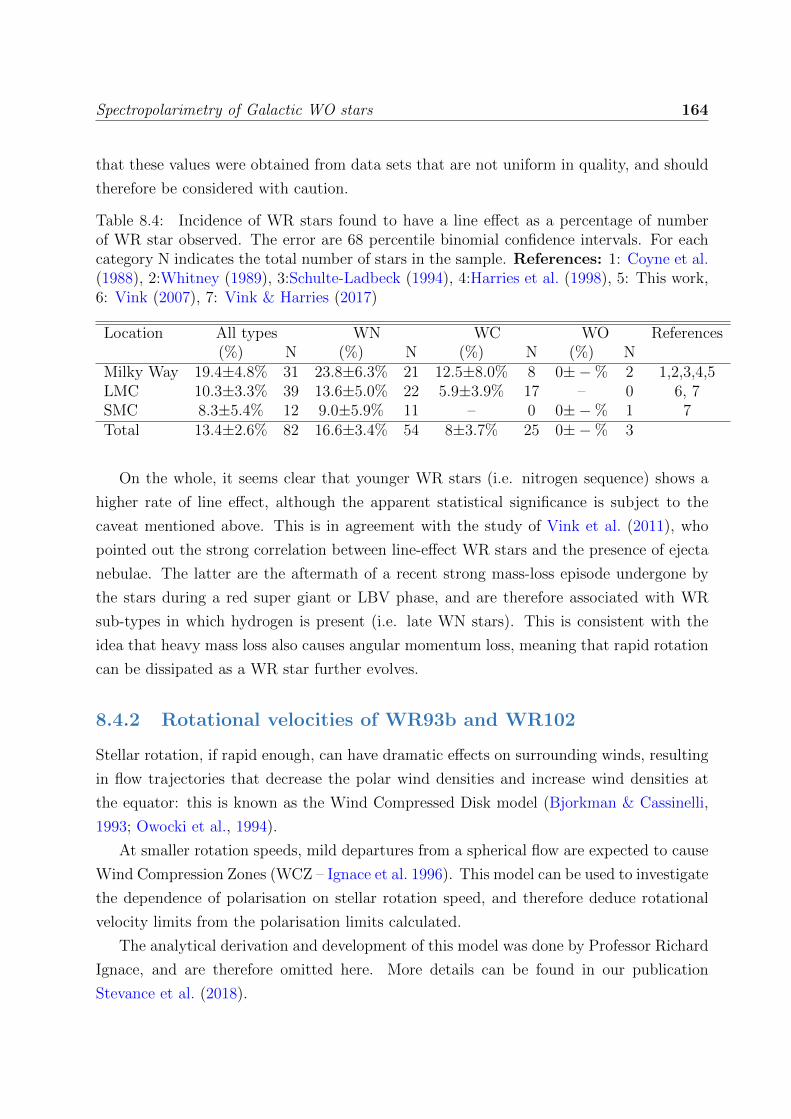
Spectropolarimetry of Galactic WO stars 164
that these values were obtained from data sets that are not uniform in quality, and should
therefore be considered with caution.
Table 8.4: Incidence of WR stars found to have a line effect as a percentage of numberof WR star observed. The error are 68 percentile binomial confidence intervals. For eachcategory N indicates the total number of stars in the sample. References: 1: Coyne et al.(1988), 2:Whitney (1989), 3:Schulte-Ladbeck (1994), 4:Harries et al. (1998), 5: This work,6: Vink (2007), 7: Vink & Harries (2017)
Location All types WN WC WO References(%) N (%) N (%) N (%) N
Milky Way 19.4±4.8% 31 23.8±6.3% 21 12.5±8.0% 8 0±−% 2 1,2,3,4,5LMC 10.3±3.3% 39 13.6±5.0% 22 5.9±3.9% 17 – 0 6, 7SMC 8.3±5.4% 12 9.0±5.9% 11 – 0 0±−% 1 7Total 13.4±2.6% 82 16.6±3.4% 54 8±3.7% 25 0±−% 3
On the whole, it seems clear that younger WR stars (i.e. nitrogen sequence) shows a
higher rate of line effect, although the apparent statistical significance is subject to the
caveat mentioned above. This is in agreement with the study of Vink et al. (2011), who
pointed out the strong correlation between line-effect WR stars and the presence of ejecta
nebulae. The latter are the aftermath of a recent strong mass-loss episode undergone by
the stars during a red super giant or LBV phase, and are therefore associated with WR
sub-types in which hydrogen is present (i.e. late WN stars). This is consistent with the
idea that heavy mass loss also causes angular momentum loss, meaning that rapid rotation
can be dissipated as a WR star further evolves.
8.4.2 Rotational velocities of WR93b and WR102
Stellar rotation, if rapid enough, can have dramatic effects on surrounding winds, resulting
in flow trajectories that decrease the polar wind densities and increase wind densities at
the equator: this is known as the Wind Compressed Disk model (Bjorkman & Cassinelli,
1993; Owocki et al., 1994).
At smaller rotation speeds, mild departures from a spherical flow are expected to cause
Wind Compression Zones (WCZ – Ignace et al. 1996). This model can be used to investigate
the dependence of polarisation on stellar rotation speed, and therefore deduce rotational
velocity limits from the polarisation limits calculated.
The analytical derivation and development of this model was done by Professor Richard
Ignace, and are therefore omitted here. More details can be found in our publication
Stevance et al. (2018).

Spectropolarimetry of Galactic WO stars 165
Figure 8.3: Relation between polarisation and rotational velocity for WR93b (blue), andWR102 (red). The dashed lines represents 1 σ limits. The polarisation limits derivedin Section 8.3.4 are marked by the open circles while the polarisation limits scaled by< sin i >2 are represented by the star markers.

Spectropolarimetry of Galactic WO stars 166
The WCZ models provide a prediction of the net linear polarisation as a function of
wrot = vrot/v∞. Terminal wind speeds of 5000 km s−1 are reported for both WR93b and
WR102 (Tramper et al., 2015), and were used to obtain the solid lines shown on Figure 8.3.
Note that the curve is for a model that assumes the axisymmetric wind is viewed edge-on.
This configuration maximises the observed polarisation and therefore minimises the limit
placed on the rotation velocity. Although it is unlikely for either WR93b or WR102 to
be edge-on systems, it is also unlikely that either (or that both) would be observed near
pole-on. Therefore, in addition to considering the calculated polarisation limits (which
represent the edge on case), the polarisation limits found in Section 8.3.4 were scaled for
< sin2 i >= 0.75 to represent the expected value of a star with random inclination. The
intersection of the polarisation limits and the upper limits on the curves of WR93b and
WR102 are indicated by the markers on Figure 8.3. The corresponding rotational velocities
are summarised in Table 8.5.
Table 8.5: Summary of the upper limits on the rotational velocities of WR93b and WR102obtained for a 90◦inclination and a random inclination, as well as the resulting limit onvrot/vcrit and specific angular momentum j = vrotR∗.
WR Scaled p vrot vrot/vcrit log(j)(%) (km s−1) (%) (cm2/s)
i = 90◦
93b <0.077 <324 <19 <18.0102 <0.057 <234 <10 <17.6
< sin i >93b <0.190 <457 <26 <18.1102 <0.141 <327 <14 <17.7
It should be noted that the wind compression effect as considered here does not include
the role of additional rotational effects such as gravity darkening or oblateness. For the
case of fast rotating B stars, Cranmer & Owocki (1995) found that the inclusion of these
non-radial force components would weaken the wind compression effect, which would lead
to rotational velocity underestimates of 5-10 percent. Unfortunately no similar study exists
for the specific case of WR stars and such investigation is beyond the scope of this chapter,
however considering the B star case our upper limits on rotational velocities may be even
higher if other rotational effects could be taken into account.
Lastly, it is worth pointing out that our upper limits on the rotational velocity of WR102
are much lower than the rotational velocity of ∼1000 km s−1 inferred by Sander et al. (2012)
from studying the shape of the emission lines in the spectrum. The model used by Sander
et al. (2012) used a number of assumptions and physical stellar parameters that are not

Spectropolarimetry of Galactic WO stars 167
Table 8.6: Summary of the physical parameters of WR93b and WR102 and their calculatedcritical velocities.
WR M? log(L?) R? vcrit dM� L� R� km s−1 kpc
93b 7.1+2.4−1.8 4.96± 0.22 0.39+0.11
−0.09 1734+545−415 2.3± 0.3
102 7.0+1.8−1.4 4.95± 0.17 0.23+0.05
−0.04 2286+528−429 2.6± 0.2
consistent with the present study, which could explain the difference in values. Most notably
they assumed spherical symmetry and used physical parameters significantly different from
those adopted here. Additionally, assuming a rotational velocity of 1000 km s−1for WR102
would result in vrot/vcrit = 44+10−8 percent (see Section 8.4.3) which is much greater than
observed in Galactic WR stars that did show a line effect (Harries et al., 1998). These
factors suggest that vrot = 1000 km s−1may be an overestimate for WR102, warranting a
re-evaluation of the Sander et al. approach using parameters based on Gaia DR2 distance.
8.4.3 vrot/vcrit and specific angular momentum j
In order to fairly compare the rotation of the targets to other WR stars it is useful to
consider the ratio vrot/vcrit. The values of vcrit can be calculated using
vcrit =
√GM?
R?
× (1− Γe), (8.2)
where M? is the stellar mass, R? is the stellar radius, and Γe is the Eddington factor
(Langer, 1998). Both the Eddington factor and the stellar mass are functions of the stellar
luminosity (Schaerer & Maeder, 1992; Vink et al., 2015), thus vcrit can be calculated from
the stellar luminosity (L?) and the stellar radius R?. We find Γe = 0.12 and 0.11 for WR93b
and WR102, respectively.
The recent DR2 data release of Gaia parallaxes (Luri et al., 2018) allowed new distances
to WR93b and WR102 to be calculated: 2.3 ±0.3 kpc and 2.6 ±0.2 kpc, respectively
(Rate et al. in prep). These estimates can be used to calculate updated values of stellar
parameters from the Tramper et al. values (see their table 4) which are summarised in
Table 8.6. The corresponding values of vcrit are found to be: vcrit = 1734+545−415 km s−1and
vcrit = 2286+528−429 km s−1for WR93b and WR102, respectively. The resulting limits on the
values of vrot/vcrit for a 90◦and a random inclination are also summarised in Table 8.5.
Additionally, based on the calculated upper limits of vrot for WR93b and WR102,
upper limits for their specific angular momentum (j) can be calculated and compared to

Spectropolarimetry of Galactic WO stars 168
the threshold of the collapsar scenario (j ≥ 3× 1016 cm2/s – MacFadyen & Woosley 1999)
as well as other Galactic WR stars (Grafener et al., 2012). The values of j calculated for
both targets for an inclination of 90◦and a random inclination are summarised in Table 8.5.
It is found that both limits on vrot/vcrit and j are very similar to the values calculated
for Galactic WR stars showing a line effect (Harries et al., 1998; Grafener et al., 2012).
Note that the rotational velocities inferred for the WR stars in Harries et al. (1998) and
Grafener et al. (2012) were calculated using spectroscopic and photometric variability,
which rely on fewer assumptions than the method employed here and are therefore more
robust. We can see that the limits placed on j for our WO stars exceed the threshold
for the collapsar model, and therefore cannot exclude WR93b and WR102 being LGRB
progenitors. However LGRBs are seen to prefer low metallicity environments (Graham &
Fruchter, 2013), making this scenario highly unlikely.
Finally, these results indicate that the absence of a line effect is not necessarily synony-
mous of insignificant rotation. When investigating the presence of rotation of WR stars
using spectropolarimetry, caution is therefore required when interpreting non detections as
the absence of a line effect is not a direct measure of the absence of rapid rotation.
8.5 Conclusions
This chapter presented FORS1 spectropolarimetric data of WR93b and WR102, which is
the first spectropolarimetric data set obtained for Galactic WO stars. The main results of
this work are:
1) No line effect is found for either WR93b and WR102.
2) Upper limits for continuum polarisation of Pcont < 0.077 percent and Pcont < 0.057
percent were deduced for WR93b and WR102, respectively.
3) The corresponding upper limits on the rotational velocity for an edge-on case and
a velocity law β = 1 are vrot < 324 km s−1and vrot < 234 km s−1, for WR93b and
WR102, respectively.
4) Upper limits on vrot/vcrit were found: <19 percent and <10 percent for WR93b and
WR102, respectively.
5) Lastly we calculated upper bounds for the specific angular momentum of WR93b
and WR102: log(j)<18.0 and log(j)<17.6 (cm2/s), respectively. These values do
not exclude the collapsar model and therefore it is not possible to constrain the

Spectropolarimetry of Galactic WO stars 169
fate of WR93b and WR102, although the preference of LGRBs for low-metallicity
environment makes this outcome highly unlikely.
The upper limits on vrot/vcrit and log(j) were found to be similar to values found for
Galactic WR stars showing a prominent line effect. Consequently this shows that the
absence of a line effect is not necessarily synonymous with the absence of rapid rotation.

Chapter 9
Conclusions
170

Conclusions 171
In this last chapter we summarise the work presented in this thesis, offer some general
remarks on our findings and briefly address future prospects.
9.1 Summary of the new supernova spectropolarimet-
ric data sets
For over 30 years now, spectropolarimetry has been a fantastic technique to probe to the
geometry of CCSNe. Spectropolarimetric observations, however, are challenging. Conse-
quently the number of multi-epoch spectropolarimetric data sets for CCSNe remains low:
only a dozen in the past three decades (see Table 1.1). The work presented in this thesis
includes multi-epoch data for three new SNe, therefore increasing this sample by 20 per-
cent. The type IIb SN 2008aq was observed at two epochs (+16 days and +27 days after
explosion), while we obtained 7 epochs of spectropolarimetry for both the type IIb SN
2011hs (from −3 days to +40 days with respect to V band maximum) and the type Ic-bl
SN 2014ad (from −2 days to +66 days with respect to V band maximum). Furthermore,
the latter is to the best of our knowledge the most exhaustive data set obtained for a SN
of this type up to this point.
9.1.1 Type IIb SN 2008aq and SN 2011hs
In Chapter 3, we found that SN 2008aq exhibited a low degree of continuum polarisation
at the first epoch (p∼0.2 percent). By the second epoch, the helium spectral features had
significantly strengthened, and the continuum polarisation had risen to (p∼1.3 percent).
Additionally, the q− u plots of SN 2008aq showed very little elongation at the first epoch,
but a clear dominant axis by +27 days after explosion. These results show a departure
from sphericity that increased significantly as the photosphere receded to the deeper part
of the ejecta into the helium layers. This is similar to the behaviour observed in SN 2001ig
(Maund et al., 2007).
On the q − u plane, the spectropolarimetric line features of Hα and He iλ5876 develop
clear loops at +27 days. This demonstrates a departure from axial symmetry. Additionally,
while the loop of helium evolves clockwise on the q−u plot, the hydrogen loop shows an anti-
clockwise rotation. Consequently, the geometrical effects causing these loops are distinct
and reveal line-specific asymmetries. These could be caused by partial obscuration of an
ellipsoidal photosphere by clumpy line forming regions.
The case of SN 2011hs (see Chapter 4) was substantially different from that of SN

Conclusions 172
2008aq. Significant continuum polarisation was detected at the first two epochs (p =
0.55±0.12 percent and p = 0.75±0.11 percent at−3 and +2 days, respectively). As opposed
to SN 2008aq, whose polarisation increased to > 1 percent as helium lines strengthened, the
continuum polarisation of SN 2011hs decreased by ∼0.25 percent +10 days after V-band
maximum, and further declined by +18 days. This is reminiscent of SN 2011dh, whose
continuum polarisation was ∼0.45 percent at 11 and 6 days before V-band maximum, but
then decreased down to p < 0.2 percent by +8 days.
The continuum polarisation of SN 2011hs also showed a progressive rotation from epoch
2 to 4 (after which the continuum P.A. could not be evaluated precisely). This was inter-
preted as the presence of a third axis coming into play causing a break from bi-axial
geometry. The rotation of the continuum P.A. was followed by that of helium, hydro-
gen and calcium line features, indicating that global geometry significantly impacted the
line polarisation. One possible interpretation is the presence of an off-axis energy source
present deep within the ejecta at early days, below an ellipsoidal photosphere (which is
bi-axial). As the photosphere recedes, the off-axis energy source would become exposed
over time, causing the continuum and line polarisation to rotate. A correlation between
helium, hydrogen and continuum P.A. was also observed for SN 2011dh, and the preferred
interpretation of Mauerhan et al. (2015) was that of nickel plumes coming from the centre
of the ejecta. Asymmetric nickel distributions could also be the off-axis energy source we
refer to in the case of SN 2011hs.
Furthermore, the distinct evolution of the hydrogen, helium and calcium loops over
time in SN 2011hs indicates that line specific geometries are also a contributor to the line
polarisation, in addition to the effects of the global geometry. Anisotropic distributions of
the line forming regions causing partial occultation of the photosphere could therefore also
be present in SN 2011hs.
On the whole, these two data sets (i.e. SN 2008aq and SN 2011hs) exhibit very different
behaviours and reveal drastically different geometries. This brings further evidence that
the spectropolarimetry of type IIb SNe, and their geometry, can vary significantly on a
case by case basis.
9.1.2 Type Ic-bl SN 2014ad
In Chapter 7 we presented the spectropolarimetric data for the type Ic-bl SN 2014ad.
The spectropolarimetric line features were extremely broadened by the very high ejecta
velocities (∼30,000 km s−1at −2 days), making line identification difficult. We were also
not able to isolate a region of the spectrum devoid of strong lines to measure the continuum
Conclusions 173
polarisation.
Overall, the degree of polarisation is seen to go down over time, and the clear dominant
axis visible on the q−u plots at the first epoch becomes significantly less prominent epoch
after epoch. Therefore, we can still conclude that the outer ejecta has significant global
elongation and becomes more spherical towards the centre. Additionally, the [O i] line at
107 days after V-band maximum shows a flat topped profile, centred on the rest wavelength
of the line, which is characteristic of the presence of a spherical oxygen shell in the deep
ejecta.
The evolution of the polarisation associated with oxygen and calcium on the q−u plots
between −2 days and +18 days shows that they arise from very distinct geometries. This
suggests that the line forming regions are clumpy and anisotropically distributed at different
depths. Oxygen is seen to evolve earlier than calcium, when the photosphere probes parts
of the ejecta further out. Furthermore, the calculated oxygen velocities are higher than that
of calcium. We concluded that the ’onion’ layer of the progenitor is partially conserved in
SN 2014ad, and that the calcium likely originated from nucleosynthesis.
Our spectropolarimetric analysis did not allow us to conclude whether SN 2014ad did or
did not have jets, although the distributions of the oxygen and calcium layers was consistent
with jet-driven explosion models of Couch et al. (2011).
9.2 The challenge of determining the ISP
Quantifying the ISP is a crucial step to retrieving the intrinsic polarisation of the object of
interest, and was very important to the analysis of the above studies. Over the past three
decades, and in this thesis, a number of methods have been used, most of them involving
the assumption that some part of the spectrum is completely depolarised.
Using the polarisation associated with the Hα emission component as a proxy for ISP is
a technique that was used in the case of SN 1993J by Trammell et al. (1993) and Tran et al.
(1997), and that we employed in Chapter 3 for SN 2008aq. Unfortunately, the assumption
of complete depolarisation in the Hα emission has previous been shown to not necessarily be
accurate (Tanaka et al., 2009). In the case of SN 2008aq, the ISP corrected data exhibited
very unexpected behaviours that were most likely the result of an inaccurate ISP estimate.
For this particular SN, the ISP was very low, and therefore it was possible to work with
ISP uncorrected data.
This is not always the case, however. In SN 2011hs, the SN polarisation features
were only revealed once the ISP had been removed. In such cases, being able to reliably

Conclusions 174
determine the interstellar component is not only important, it is essential to being able to
perform a subsequent analysis. A number of methods were attempted to estimate the ISP
in the data of SN 2011hs. We tried to decompose the polarisation of strong emission lines to
separate the continuum polarisation from the line polarisation. Under the assumption that
intrinsic line polarisation is zero, the values found for its component would actually reveal
the ISP. Even if this assumption was completely valid, the method requires an estimate of
the continuum flux across a line, and this is extremely difficult to do accurately. In the
end, we were not able to obtain results from this technique.
Another approach is to consider the strong emission lines at late time. The decrease
in intrinsic continuum flux and polarisation at these dates rendered the assumption that
line polarisation equated to ISP more robust. This was successfully used in SN 2014ad
by averaging the stokes parameters in the strong emission line regions. In SN 2011hs, we
fitted a line through the data points associated with the strong emission lines to obtain
an ISP estimate. This was also satisfactory, although the errors on the fit were quite large
and propagated to the ISP corrected data.
The final method used to remove the ISP of SN 2011hs was to fit with a straight line the
spectropolarimetric data at the last epoch across the whole spectrum, using sigma clipping
to remove outliers. This is independent of any assumption on the emission lines, but only
works if the fitted data is taken at an epoch were the intrinsic SN polarisation is negligible
compared to that induced by the ISM.
One last approach mentioned in this thesis was the use of the spectral region affected
by line blanketing (blue parts of the spectrum ∼5000A). This was used in SN 2014ad
successfully, but one major caveat to this method is that it cannot be used reliably if line
polarisation arises in this region of the spectrum (e.g. see SN 2008aq at +27 days and
Table 6.3).
On the whole, estimating the ISP is difficult. All methods rely on assumptions, and
they cannot be universally used without some degree of healthy scepticism. In some cases
were the ISP is low, like SN 2008aq or SN 2011dh, it is preferable not to attempt to remove
the ISP, since a wrong estimate can severely impact the data (see Chapter 3, Mauerhan
et al. 2015).

Conclusions 175
9.3 To use or not to use a toy model: that is the
question
In order to further interpret the observed spectropolarimetry of SN and provide a more
detailed picture of their ejecta, models are required. Fully hydrostatic models with radiative
transfer are not yet available. Monte Carlo toy models have been used in the past by Maund
et al. (2010), and Reilly et al. (2016, 2017) as a way to provide insight on the geometries
resulting in the observed polarisation. Unfortunately, these models were used without
performing a full exploration of parameter space, and one of our main goals was to do this
methodically to understand the range of possible solutions to a given observation.
These toy models are two dimensional and work under a number of assumptions. An
ellipsoidal photosphere (surface of last scattering) is created by randomly generating photon
packets and attributing each of them a luminosity and a polarisation according to their
position. Some fine tuning is required for the polarisation of a photosphere with a given axis
ratio to reproduce the results of more exhaustive models such as those of Hoflich (1991).
The full set of formulae used can be found in Chapter 5.
Line polarisation in these models is only considered to arise from partial obscuration,
and therefore do not take into account the potential effects of global geometry on line
polarisation (see Section 1.3.2). Line forming regions are placed in front of the photosphere,
and are given a very high optical depth such that all the underlying photon packets are
removed from subsequent calculations. In our models we used one circular line forming
region, described by 3 parameters: its radius (r) and the Cartesian coordinates of its
centre (x, y). After applying our line forming region to our ellipsoidal photosphere we
averaged the Stokes parameters q and u, and calculated the ratio of the flux after line
absorption to the total (i.e. continuum) flux. This could then be compared to the values
observed in the data. Note that the models of Reilly et al. (2016, 2017) included more
complex geometries. As a first approach, however, we focused on the most simple case
(a single circular absorption region), as one of our goals was to explore parameter space
methodically.
In order to do this, we used a grid-search approach and created look-up tables to
summarise the Stokes parameters and flux ratio simulated for each set of three parameters.
Observations could then be compared to these values. Because it would have been overly
time consuming to create a fine enough grid to provide 1σ solutions to all our observations,
we first isolated the region of parameter space, including 3σ solutions, and then ran more
models with a finer grid focused on that particular region of parameter space.

Conclusions 176
We used our models on the helium, hydrogen and calcium data of SN 2011hs from −3
to +10 days (see Chapter 5). Although solutions were found for all the observables we at-
tempted to model, we also found a great number of degeneracies. Even more degeneracies
would occur if more parameters were considered. This is a concern for previous models
that did not fully explore parameter space whilst using more complex geometries. Addi-
tionally, we also found good solutions at +10 days, although our analysis of SN 2011hs in
Chapter 4 revealed that the global geometry was tri-axial rather than bi-axial, invalidat-
ing the assumption that the photosphere can be represented as a simple projected ellipse.
Consequently, this type of toy model can be misleading and should be used with great care,
if at all.
9.4 Spectropolarimetry of WO stars and progenitor
link
Spectropolarimetry has been used extensively to study the asymmetries of WR star winds.
The presence of a line effect (peaks or troughs associated with strong emission lines) has
been used as a proxy for rapid rotation, as a wind distorted by rapid rotation would yield
net continuum polarisation.
In Chapter 8, we studied for the first time the spectropolarimetry of two Galactic WO
stars: WR93b and WR102. WO stars in particular are candidate progenitors for type
Ic-bl SNe, and the collapsar model by which they are thought to create these SNe requires
enough angular momentum to power the central engine (MacFadyen & Woosley, 1999)
We found no line effect in either WR93b nor WR102. We used a Serkowski law fit to
the data to remove the contribution of the ISP and continuum, to help us place upper
limits on the detectability of the line effect. This in turn allowed us to derive upper limits
for the continuum polarisation of Pcont < 0.077 percent and Pcont < 0.057 for WR93b and
WR102, respectively.
Using an analytical model by Richard Ignace (private communications), we then con-
strained the rotational velocity to vrot < 324 km s−1and vrot < 234 km s−1, for WR93b
and WR102, respectively. Note that this is for an edge-on case and a velocity law β = 1.
These values correspond to upper limits on vrot/vcrit of <19 percent and <10 percent for
WR93b and WR102, respectively. Additionally, from the above rotational velocities we can
derive limits on the specific angular momentum of log(j)<18.0 and log(j)<17.6 (cm2/s),
for WR93b and WR102 respectively. These are not sufficient to exclude the possibility of
a collapsar event, and we could not further constrain the fate of WR93b and WR102.

Conclusions 177
Lastly, the upper limits on vrot/vcrit and log(j) were found to be similar to values found
for Galactic WR stars showing a prominent line effect. Consequently this shows that the
absence of a line effect is not necessarily synonymous with the absence of rapid rotation.
9.5 Future work
In addition to the work summarised in the previous sections, we also provided a new
estimate of the ISP of SN 1993J and preliminary re-analysis of its spectropolarimetric
data (see Chapter 6). Further analysis is required and discussions are on-going with my
collaborators.
As mentioned previously, one of the main road-blocks to exhaustively interpreting SN
spectropolarimetry is the need for better modelling. 3D hydrostatic models with radiative
transfer that can reproduce both the polarisation and the flux spectra will be the key to
extracting more information from the spectropolarimetric data sets already in the literature,
and the ones to come in the future.
On the whole, the number of multi-epoch data sets available for CCSNe still remains
limited, now counting 15 objects. It would be beneficial to obtain time coverage at a higher
cadence as it would offer better depth resolution. Additionally, being able to follow up SNe
very soon after explosion will be made easier by initiatives such as the Zviky Transient
Factory and the Large Synoptic Survey Telescope. Currently, SN 2008ax is our earliest
sample, observed only 6 days after explosion.
The fact that we are now finding SNe at a greater rate than ever before, however,
will not necessarily result in a dramatic increase in the number of high-quality multi-epoch
spectropolarimetric data sets. Indeed, these observations remain very challenging, requiring
long exposure times, even on 8 meter class telescopes. Additionally, spectropolarimetric
analysis is difficult, particularly the ISP removal process. This will require a lot of human
input and is not easily automated. On the whole, although spectropolarimetry is a very
useful technique, the diversity seen in the currently available data shows that a much larger
sample will be required to find global trends within and across SN sub-types. This will be
challenging, and will require an observing and analysis strategy that is scalable to the new
era of Big Data Astronomy.

Bibliography
Anderson C. M., Weitenbeck A. J., Code A. D., Nordsieck K. H., Meade M. R., BablerB. L., Zellner N. E. B., Bjorkman K. S., Fox G. K., Johnson J. J., Sanders W. T., LupieO. L., Edgar R. J., 1996, AJ, 112, 2726
Appenzeller I., Fricke K., Furtig W., Gassler W., Hafner R., Harke R., Hess H.-J., HummelW., Jurgens P., Kudritzki R.-P., 1998, The Messenger, 94, 1
Bianco F. B., Modjaz M., Hicken M., Friedman A., Kirshner R. P., Bloom J. S., ChallisP., Marion G. H., Wood-Vasey W. M., Rest A., 2014, ApJS, 213, 19
Bjorkman J. E., Cassinelli J. P., 1993, ApJ, 409, 429
Blondin J. M., Mezzacappa A., DeMarino C., 2003, ApJ, 584, 971
Branch D., Benetti S., Kasen D., Baron E., Jeffery D. J., Hatano K., Stathakis R. A.,Filippenko A. V., Matheson T., Pastorello A., Altavilla G., Cappellaro E., Rizzi L.,Turatto M., Li W., Leonard D. C., Shields J. C., 2002, ApJ, 566, 1005
Branch D., Wheeler J. C., 2017, Supernova Explosions
Bromberg O., Nakar E., Piran T., 2011, ApJL, 739, L55
Bufano F., Pignata G., Bersten M., Mazzali P. A., Ryder S. D., Margutti R., MilisavljevicD., Morelli L., Benetti S., Cappellaro E., Gonzalez-Gaitan S., Romero-Canizales C.,2014, MNRAS, 439, 1807
Burrows A., Livne E., Dessart L., Ott C. D., Murphy J., 2006, ApJ, 640, 878
Callingham J. R., Tuthill P. G., Pope B. J. S., Williams P. M., Crowther P. A., EdwardsM., Norris B., Kedziora-Chudczer L., 2018, Nature Astronomy
Cardelli J. A., Clayton G. C., Mathis J. S., 1989, ApJ, 345, 245
Chandrasekhar 1960, Principles of Stellar dynamics. New York: Dover
Chatterjee S., Vlemmings W. H. T., Brisken W. F., Lazio T. J. W., Cordes J. M., GossW. M., Thorsett S. E., Fomalont E. B., Lyne A. G., Kramer M., 2005, ApJL, 630, L61
178

Conclusions 179
Chornock R., Berger E., Levesque E. M., Soderberg A. M., Foley R. J., Fox D. B., FrebelA., Simon J. D., Bochanski J. J., Challis P. J., Kirshner R. P., Podsiadlowski P., RothK., Rutledge R. E., Schmidt B. P., Sheppard S. S., Simcoe R. A., 2010, ArXiv e-prints
Chornock R., Filippenko A. V., Li W., Marion G. H., Foley R. J., Modjaz M., Rafelski M.,Becker G. D., de Vries W. H., Garnavich P., Jorgenson R. A., 2011, ApJ, 739, 41
Chu J., Li W., Filippenko A. V., Blondin S., Narayan G., 2008, Central Bureau ElectronicTelegrams, 1271
Chugai N. N., 1992, Soviet Astronomy Letters, 18, 168
Cikota A., Patat F., Cikota S., Spyromilio J., Rau G., 2017, MNRAS, 471, 2111
Cordes J. M., Chernoff D. F., 1998, ApJ, 505, 315
Couch S. M., Pooley D., Wheeler J. C., Milosavljevic M., 2011, ApJ, 727, 104
Coyne G. V., 1974, AJ, 79, 565
Coyne G. V., Gehrels T., 1966, AJ, 71, 355
Coyne G. V., Magalhaes A. M., Moffat A. F., Schulte-Ladbeck R. E., Tapia S., 1988,Polarized radiation of circumstellar origin
Cranmer S. R., Owocki S. P., 1995, ApJ, 440, 308
Cropper M., Bailey J., McCowage J., Cannon R. D., Couch W. J., Walsh J. R., StradeJ. O., Freeman F., 1988, MNRAS, 231, 695
Crowther P. A., 2007, ARAA, 45, 177
Crowther P. A., 2013, MNRAS, 428, 1927
del Toro Iniesta J. C., 2003, Introduction to Spectropolarimetry
Dessart L., Hillier D. J., Livne E., Yoon S.-C., Woosley S., Waldman R., Langer N., 2011,MNRAS, 414, 2985
Djorgovski S. G., Drake A. J., Mahabal A. A., Graham M. J., Donalek C., Williams R.,Beshore E. C., Larson S. M., Prieto J., Catelan M., Christensen E., McNaught R. H.,2011, ArXiv e-prints
Drew J. E., Barlow M. J., Unruh Y. C., Parker Q. A., Wesson R., Pierce M. J., MashederM. R. W., Phillipps S., 2004, MNRAS, 351, 206
Eldridge J. J., Izzard R. G., Tout C. A., 2008, MNRAS, 384, 1109
Ferguson A. M. N., Gallagher J. S., Wyse R. F. G., 1998, AJ, 116, 673
Filippenko A. V., 1988, AJ, 96, 1941

Conclusions 180
Filippenko A. V., 1997, ARAA, 35, 309
Filippenko A. V., Matheson T., Ho L. C., 1993, ApJL, 415, L103
Fox O. D., Azalee Bostroem K., Van Dyk S. D., Filippenko A. V., Fransson C., MathesonT., Cenko S. B., Chandra P., Dwarkadas V., Li W., Parker A. H., Smith N., 2014, ApJ,790, 17
Gal-Yam A., Leonard D. C., 2009, Nature, 458, 865
Garnavich P. M., Stanek K. Z., Wyrzykowski L., Infante L., Bendek E., Bersier D., HollandS. T., Jha S., Matheson T., Kirshner R. P., Krisciunas K., Phillips M. M., Carlberg R. G.,2003, ApJ, 582, 924
Grafener G., Vink J. S., Harries T. J., Langer N., 2012, A&A, 547, A83
Graham J. F., Fruchter A. S., 2013, ApJ, 774, 119
Graham J. F., Fruchter A. S., 2015, ArXiv e-prints
Hachinger S., Mazzali P. A., Taubenberger S., Hillebrandt W., Nomoto K., Sauer D. N.,2012, MNRAS, 422, 70
Hammer F., Flores H., Schaerer D., Dessauges-Zavadsky M., Le Floc’h E., Puech M., 2006,A&A, 454, 103
Han Z., Podsiadlowski P., 2004, MNRAS, 350, 1301
Harries T. J., Hillier D. J., Howarth I. D., 1998, MNRAS, 296, 1072
Heiles C., 2000, AJ, 119, 923
Hensler G., 2011, in Alves J., Elmegreen B. G., Girart J. M., Trimble V., eds, Com-putational Star Formation Vol. 270 of IAU Symposium, Supernova Feedback on theInterstellar Medium and Star Formation. pp 309–317
Ho L. C., Li Z.-Y., Barth A. J., Seigar M. S., Peng C. Y., 2011, ApJS, 197, 21
Hoang T., 2017, ApJ, 836, 13
Hoang T., Tram L. N., Lee H., Ahn S.-H., 2018, ArXiv e-prints
Hoflich P., 1991, A&A, 246, 481
Hoflich P., 1995, ApJ, 440, 821
Hoflich P., Wheeler J. C., Wang L., 1999, ApJ, 521, 179
Howell D. A., Hoflich P., Wang L., Wheeler J. C., 2001, ApJ, 556, 302

Conclusions 181
Howerton S., Drake A., Djorgovski S., Mahabal A., Graham M., Williams R., Prieto J.,Catelan M., Christensen E., Larson S. M., 2014, CBAT, 3831
Howerton S. C., , 2017, CRTS SNHunt: The first five years of supernova discoveries, self-published on http://www.lulu.com/
Ignace R., Brimeyer A., 2006, MNRAS, 371, 343
Ignace R., Cassinelli J. P., Bjorkman J. E., 1996, ApJ, 459, 671
Ignace R., Hendry M. A., 2000, ApJL, 537, L131
Iwamoto K., Mazzali P. A., Nomoto K., Umeda H., Nakamura T., Patat F., Danziger I. J.,Young T. R., Suzuki T., Shigeyama T., Augusteijn T., Doublier V., 1998, Nature, 395,672
Iwamoto K., Nakamura T., Nomoto K., Mazzali P. A., Danziger I. J., Garnavich P., Kir-shner R., Jha S., Balam D., Thorstensen J., 2000, ApJ, 534, 660
Janka H.-T., 2012, Annual Review of Nuclear and Particle Science, 62, 407
Jeffery D. J., 1991, ApJ, 375, 264
Jones E., Oliphant T., Peterson P., et al., 2017, SciPy: Open source scientific tools forPython
Kasen D., Nugent P., Wang L., Howell D. A., Wheeler J. C., Hoflich P., Baade D., BaronE., Hauschildt P. H., 2003, ApJ, 593, 788
Kawabata K. S., Deng J., Wang L., Mazzali P., Nomoto K., Maeda K., Tominaga N.,Umeda H., Iye M., Kosugi G., Ohyama Y., Sasaki T., 2003, ApJL, 593, L19
Kawabata K. S., Jeffery D. J., Iye M., Ohyama Y., Kosugi G., Kashikawa N., Ebizuka N.,Sasaki T., Sekiguchi K., Nomoto K., Mazzali P., Deng J., Maeda K., Umeda H., AokiK., 2002, ApJL, 580, L39
Khokhlov A. M., Hoflich P. A., Oran E. S., Wheeler J. C., Wang L., Chtchelkanova A. Y.,1999, ApJL, 524, L107
Koribalski B. S., Staveley-Smith L., Kilborn V. A., Ryder S. D., Kraan-Korteweg R. C.,Ryan-Weber E. V., Ekers R. D., Jerjen H., Henning P. A., Putman M. E., 2004, AJ, 128,16
Kotake K., Sawai H., Yamada S., Sato K., 2004, ApJ, 608, 391
Kumar B., Pandey S. B., Sahu D. K., Vinko J., Moskvitin A. S., Anupama G. C., BhattV. K., Ordasi A., Nagy A., Sokolov V. V., Sokolova T. N., Komarova V. N., Kumar B.,Bose S., Roy R., Sagar R., 2013, MNRAS, 431, 308

Conclusions 182
Kunkel W., Madore B., Shelton I., Duhalde O., Bateson F. M., Jones A., Moreno B.,Walker S., Garradd G., Warner B., Menzies J., 1987, IAUC, 4316
Langer N., 1998, A&A, 329, 551
Langer N., 2012, ARAA, 50, 107
Lazzati D., Morsony B. J., Blackwell C. H., Begelman M. C., 2012, ApJ, 750, 68
Leonard D. C., Filippenko A. V., Ardila D. R., Brotherton M. S., 2001, ApJ, 553, 861
Leonard D. C., Filippenko A. V., Ganeshalingam M., Serduke F. J. D., Li W., Swift B. J.,Gal-Yam A., Foley R. J., Fox D. B., Park S., Hoffman J. L., Wong D. S., 2006, Nature,440, 505
Levesque E. M., Berger E., Kewley L. J., Bagley M. M., 2010, AJ, 139, 694
Levesque E. M., Kewley L. J., Berger E., Zahid H. J., 2010, AJ, 140, 1557
Levesque E. M., Soderberg A. M., Kewley L. J., Berger E., 2010, ApJ, 725, 1337
Li W., Leaman J., Chornock R., Filippenko A. V., Poznanski D., Ganeshalingam M., WangX., Modjaz M., Jha S., Foley R. J., Smith N., 2011, MNRAS, 412, 1441
Lim P. L., Diaz R. I., Laidler V., , 2015, PySynphot Users Guide (Baltimore, MD: STScI)
Liu Y.-Q., Modjaz M., Bianco F. B., Graur O., 2016, ApJ, 827, 90
Luri X., Brown A. G. A., Sarro L. M., Arenou F., Bailer-Jones C. A. L., Castro-Ginard A.,de Bruijne J., Prusti T., Babusiaux C., Delgado H. E., 2018, ArXiv e-prints
Lyne A. G., Lorimer D. R., 1994, Nature, 369, 127
MacFadyen A. I., Woosley S. E., 1999, ApJ, 524, 262
Maeda K., Kawabata K., Mazzali P. A., Tanaka M., Valenti S., Nomoto K., Hattori T.,Deng J., Pian E., Taubenberger S., Iye M., Matheson T., Filippenko A. V., Aoki K.,Kosugi G., Ohyama Y., Sasaki T., Takata T., 2008, Science, 319, 1220
Maeda K., Nakamura T., Nomoto K., Mazzali P. A., Patat F., Hachisu I., 2002, ApJ, 565,405
Manchester R. N., 1987, A&A, 171, 205
Martin P. G., Adamson A. J., Whittet D. C. B., Hough J. H., Bailey J. A., Kim S.-H.,Sato S., Tamura M., Yamashita T., 1992, ApJ, 392, 691
Martin P. G., Clayton G. C., Wolff M. J., 1999, ApJ, 510, 905

Conclusions 183
Mauerhan J. C., Williams G. G., Leonard D. C., Smith P. S., Filippenko A. V., Smith N.,Hoffman J. L., Huk L., Clubb K. I., Silverman J. M., Cenko S. B., Milne P., Gal-YamA., Ben-Ami S., 2015, MNRAS, 453, 4467
Maund J. R., 2008, A&A, 481, 913
Maund J. R., Smartt S. J., 2009, Science, 324, 486
Maund J. R., Smartt S. J., Kudritzki R. P., Podsiadlowski P., Gilmore G. F., 2004, Nature,427, 129
Maund J. R., Wheeler J. C., Baade D., Patat F., Hoflich P., Wang L., Clocchiatti A., 2009,ApJ, 705, 1139
Maund J. R., Wheeler J. C., Patat F., Baade D., Wang L., Hoflich P., 2007a, A&A, 475,L1
Maund J. R., Wheeler J. C., Patat F., Baade D., Wang L., Hoflich P., 2007b, MNRAS,381, 201
Maund J. R., Wheeler J. C., Patat F., Wang L., Baade D., Hoflich P. A., 2007, ApJ, 671,1944
Maund J. R., Wheeler J. C., Wang L., Baade D., Clocchiatti A., Patat F., Hoflich P.,Quinn J., Zelaya P., 2010, ApJ, 722, 1162
Mazzali P. A., Deng J., Maeda K., Nomoto K., Filippenko A. V., Matheson T., 2004, ApJ,614, 858
Mazzali P. A., Deng J., Maeda K., Nomoto K., Umeda H., Hatano K., Iwamoto K., YoshiiY., Kobayashi Y., Minezaki T., Doi M., Enya K., 2002, ApJL, 572, L61
Mazzali P. A., Foley R. J., Deng J., Patat F., Pian E., Baade D., Bloom J. S., FilippenkoA. V., Perley D. A., Valenti S., Wang L., Kawabata K., Maeda K., Nomoto K.-i., 2007,ApJ, 661, 892
McGlynn S., Clark D. J., Dean A. J., Hanlon L., McBreen S., Willis D. R., McBreen B.,Bird A. J., Foley S., 2007, A&A, 466, 895
Milisavljevic D., Fesen R., Soderberg A., Pickering T., Kotze P., 2011, Central BureauElectronic Telegrams, 2902, 2
Milisavljevic D., Fesen R. A., Gerardy C. L., Kirshner R. P., Challis P., 2010, ApJ, 709,1343
Minkowski R., 1941, PASP, 53, 224
Modjaz M., Blondin S., Kirshner R. P., Matheson T., Berlind P., Bianco F. B., CalkinsM. L., Challis P., Garnavich P., Hicken M., Jha S., Liu Y. Q., Marion G. H., 2014, AJ,147, 99

Conclusions 184
Modjaz M., Kewley L., Bloom J. S., Filippenko A. V., Perley D., Silverman J. M., 2011,ApJL, 731, L4
Modjaz M., Kewley L., Kirshner R. P., Stanek K. Z., Challis P., Garnavich P. M., GreeneJ. E., Kelly P. L., Prieto J. L., 2008, AJ, 135, 1136
Modjaz M., Liu Y. Q., Bianco F. B., Graur O., 2016, ApJ, 832, 108
Munari U., Barbon R., Piemonte A., Tomasella L., Rejkuba M., 1998, A&A, 333, 159
Nomoto K., Suzuki T., Shigeyama T., Kumagai S., Yamaoka H., Saio H., 1993, Nature,364, 507
Owocki S. P., Cranmer S. R., Blondin J. M., 1994, ApJ, 424, 887
Patat F., Cappellaro E., Danziger J., Mazzali P. A., Sollerman J., Augusteijn T., BrewerJ., Doublier V., Gonzalez J. F., Hainaut O., Lidman C., Leibundgut B., 2001, ApJ, 555,900
Patat F., Romaniello M., 2006, PASP, 118, 146
Patat F., Taubenberger S., Cox N. L. J., Baade D., Clocchiatti A., Hoflich P., Maund J. R.,Reilly E., Spyromilio J., Wang L., Wheeler J. C., Zelaya P., 2015, A&A, 577, A53
Perley D. A., Kruhler T., Schady P., Micha lowski M. J., Thone C. C., Petry D., GrahamJ. F., Greiner J., Klose S., Schulze S., Kim S., 2017, MNRAS, 465, L89
Pettini M., Pagel B. E. J., 2004, MNRAS, 348, L59
Podsiadlowski P., Hsu J. J. L., Joss P. C., Ross R. R., 1993, Nature, 364, 509
Poznanski D., Prochaska J. X., Bloom J. S., 2012, MNRAS, 426, 1465
Prentice S. J., Ashall C., James P. A., Short L., Mazzali P. A., Bersier D., Crowther P. A.,Barbarino C., Chen T.-W., Copperwheat C. M., Darnley M. J., Denneau L., Elias-Rosa., 2019, MNRAS, 485, 1559
Price P. A., Kulkarni S. R., Berger E., Djorgovski S. G., Frail D. A., Mahabal A., FoxD. W., Harrison F. A., Bloom J. S., Yost S. A., Reichart D. E., Henden A. A., RickerG. R., van der Spek R., Hurley K., Atteia J.-L., Kawai N., Fenimore E., Graziani C.,2002, ApJL, 571, L121
Reilly E., Maund J. R., Baade D., Wheeler J. C., Hoflich P., Spyromilio J., Patat F., WangL., 2017, MNRAS, 470, 1491
Reilly E., Maund J. R., Baade D., Wheeler J. C., Silverman J. M., Clocchiatti A., PatatF., Hoflich P., Spyromilio J., Wang L., Zelaya P., 2016, MNRAS, 457, 288
Richardson D., Branch D., Baron E., 2006, AJ, 131, 2233

Conclusions 185
Sahu D. K., Anupama G. C., Chakradhari N. K., Srivastav S., Tanaka M., Maeda K.,Nomoto K., 2018, MNRAS, 475, 2591
Sana H., de Mink S. E., de Koter A., Langer N., Evans C. J., Gieles M., Gosset E., IzzardR. G., Le Bouquin J.-B., Schneider F. R. N., 2012, Science, 337, 444
Sander A., Hamann W.-R., Todt H., 2012, A&A, 540, A144
Sanders N. E., Soderberg A. M., Levesque E. M., Foley R. J., Chornock R., MilisavljevicD., Margutti R., Berger E., Drout M. R., Czekala I., Dittmann J. A., 2012, ApJ, 758,132
Scannapieco C., Tissera P. B., White S. D. M., Springel V., 2008, MNRAS, 389, 1137
Schaerer D., Maeder A., 1992, A&A, 263, 129
Schlafly E. F., Finkbeiner D. P., 2011, ApJ, 737, 103
Schlegel E. M., 1990, MNRAS, 244, 269
Schulte-Ladbeck R. E., 1994, Ap&SS, 221, 347
Schulte-Ladbeck R. F., Nordsieck K. H., Taylor M., Bjorkman K. S., Magalhaes A. M.,Wolff M. J., 1992, ApJ, 387, 347
Schulze S., Malesani D., Cucchiara A., Tanvir N. R., Kruhler T., de Ugarte Postigo A.,Leloudas G., Lyman J., Bersier D., Wiersema K., Perley D. A., 2014, A&A, 566, A102
Serkowski K., 1973, in Greenberg J. M., van de Hulst H. C., eds, Interstellar Dust andRelated Topics Vol. 52 of IAU Symposium, Interstellar Polarization (review). p. 145
Serkowski K., Mathewson D. S., Ford V. L., 1975, ApJ, 196, 261
Shapiro P. R., Sutherland P. G., 1982, ApJ, 263, 902
Shivvers I., Modjaz M., Zheng W., Liu Y., Filippenko A. V., Silverman J. M., MathesonT., Pastorello A., Graur O., Foley R. J., Chornock R., Smith N., Leaman J., Benetti S.,2017, PASP, 129, 054201
Silverman J. M., Mazzali P., Chornock R., Filippenko A. V., Clocchiatti A., Phillips M. M.,Ganeshalingam M., Foley R. J., 2009, PASP, 121, 689
Smartt S. J., 2009, ARAA, 47, 63
Smith N., Li W., Filippenko A. V., Chornock R., 2011, MNRAS, 412, 1522
Soderberg A. M., Nakar E., Berger E., Kulkarni S. R., 2006, ApJ, 638, 930
Sollerman J., Jaunsen A. O., Fynbo J. P. U., Hjorth J., Jakobsson P., Stritzinger M., FeronC., Laursen P., Ovaldsen J.-E., Selj J., Thone C. C., 2006, A&A, 454, 503

Conclusions 186
Sollerman J., Ostlin G., Fynbo J. P. U., Hjorth J., Fruchter A., Pedersen K., 2005, NewAstronomy, 11, 103
Spyromilio J., 1994, MNRAS, 266, L61
St.-Louis N., Drissen L., Moffat A. F. J., Bastien P., Tapia S., 1987, ApJ, 322, 870
Stanek K. Z., Matheson T., Garnavich P. M., Martini P., Berlind P., Caldwell N., ChallisP., Brown W. R., Schild R., Krisciunas K., Calkins M. L., 2003, ApJL, 591, L17
Stevance H. F., Ignace R., Crowther P. A., Maund J. R., Davies B., Rate G., 2018, MNRAS,479, 4535
Stevance H. F., Maund J. R., Baade D., Bruten J., Cikota A., Hoflich P., Wang L., WheelerJ. C., Clocchiatti A., Spyromilio J., Patat F., Yang Y., Crowther P., 2019, MNRAS
Stevance H. F., Maund J. R., Baade D., Hoflich P., Howerton S., Patat F., Rose M.,Spyromilio J., Wheeler J. C., Wang L., 2017, MNRAS, 469, 1897
Stevance H. F., Maund J. R., Baade D., Hoflich P., Patat F., Spyromilio J., Wheeler J. C.,Clocchiatti A., Wang L., Yang Y., Zelaya P., 2016, MNRAS, 461, 2019
Stritzinger M., Mazzali P., Phillips M. M., Immler S., Soderberg A., Sollerman J., BoldtL., Braithwaite J., Brown P., Burns C. R., Contreras C., 2009, ApJ, 696, 713
Swartz D. A., Clocchiatti A., Benjamin R., Lester D. F., Wheeler J. C., 1993, Nature, 365,232
Takiwaki T., Kotake K., Suwa Y., 2016, ArXiv e-prints
Tanaka M., Kawabata K. S., Maeda K., Iye M., Hattori T., Pian E., Nomoto K., MazzaliP. A., Tominaga N., 2009, ApJ, 699, 1119
Tanaka M., Maeda K., Mazzali P. A., Kawabata K. S., Nomoto K., 2017, ApJ, 837, 105
Thomas R. C., Nugent P. E., Meza J. C., 2011, PASP, 123, 237
Thone C. C., Fynbo J. P. U., Ostlin G., Milvang-Jensen B., Wiersema K., Malesani D.,Ferreira D. D. M., Gorosabel J., Kann D. A., Watson D., Micha lowski M. J., FruchterA. S., Levan A. J., Hjorth J., Sollerman J., 2008, ApJ, 676, 1151
Trammell S. R., Hines D. C., Wheeler J. C., 1993, ApJL, 414, L21
Tramper F., Grafener G., Hartoog O. E., Sana H., de Koter A., Vink J. S., EllerbroekL. E., Langer N., Garcia M., Kaper L., de Mink S. E., 2013, A&A, 559, A72
Tramper F., Straal S. M., Sanyal D., Sana H., de Koter A., Grafener G., Langer N., VinkJ. S., de Mink S. E., Kaper L., 2015, A&A, 581, A110

Conclusions 187
Tran H. D., Filippenko A. V., Schmidt G. D., Bjorkman K. S., Jannuzi B. T., Smith P. S.,1997, PASP, 109, 489
van de Hulst H. C., 1957, Light Scattering by Small Particles
Van Dyk S. D., Cenko S. B., Poznanski D., Arcavi I., Gal-Yam A., Filippenko A. V.,Silverio K., Stockton A., Cuillandre J.-C., Marcy G. W., Howard A. W., Isaacson H.,2012, ApJ, 756, 131
Van Dyk S. D., Li W., Filippenko A. V., 2003, PASP, 115, 1
Vink J. S., 2007, A&A, 469, 707
Vink J. S., de Koter A., Lamers H. J. G. L. M., 2001, A&A, 369, 574
Vink J. S., Grafener G., Harries T. J., 2011, A&A, 536, L10
Vink J. S., Harries T. J., 2017, A&A, 603, A120
Vink J. S., Heger A., Krumholz M. R., Puls J., Banerjee S., Castro N., Chen K.-J., CheneA.-N., Crowther P. A., Daminelli A., Grafener G., 2015, Highlights of Astronomy, 16, 51
Wang L., Baade D., Hoflich P., Wheeler J. C., 2003, ApJ, 592, 457
Wang L., Baade D., Patat F., 2007, Science, 315, 212
Wang L., Howell D. A., Hoflich P., Wheeler J. C., 2001, ApJ, 550, 1030
Wang L., Wheeler J. C., 2008, ARAA, 46, 433
Wang L., Wheeler J. C., Hoflich P., 1997, ApJL, 476, L27
Webbink R. F., 1984, ApJ, 277, 355
Whitney B. A., 1989, BAAS, 20, 1013
Whittet D. C. B., Martin P. G., Hough J. H., Rouse M. F., Bailey J. A., Axon D. J., 1992,ApJ, 386, 562
Wolf C. J. E., Rayet G., 1867, Academie des Sciences Paris Comptes Rendus, 65, 292
Wolstencroft R. D., Kemp J. C., 1972, Nature, 238, 452
Wong O. I., Ryan-Weber E. V., Garcia-Appadoo D. A., Webster R. L., Staveley-Smith L.,Zwaan M. A., Meyer M. J., Barnes D. G., Kilborn V. A., 2006, MNRAS, 371, 1855
Wongwathanarat A., Janka H.-T., Muller E., 2013, A&A, 552, A126
Woosley S. E., 1993, ApJ, 405, 273
Woosley S. E., Eastman R. G., Schmidt B. P., 1999, ApJ, 516, 788

Conclusions 188
Woosley S. E., MacFadyen A. I., 1999, A&A Suppl., 138, 499
Woosley S. E., Weaver T. A., 1994, ApJ, 423, 371
Yoon S.-C., 2015, PASA, 32, e015
Yoon S.-C., Grafener G., Vink J. S., Kozyreva A., Izzard R. G., 2012, A&A, 544, L11

Appendix A
Investigating the original reduction of
SN 2008aq
Unlike the data presented in Chapter 3, originally published data in Stevance et al. (2016)
were not reduced by myself using FUSS. Instead, the analysis was performed on polarisa-
tion that had been pre-reduced.
Ulteriorly, the raw data of SN 2008aq were reduced using FUSS, revealing a number
of discrepancies which brought me to investigate the original data further (details below).
The issues identified being minor, they do not affect the main conclusions of our paper,
however during the writing of this thesis I chose to move away from the original reduction
and to instead use my own; I motivate this choice in this appendix.
A.1 Discrepant values in +16 days data
The most visible difference between the original reduction and my own was the presence of
a peak in polarisation at +16 days associated with the Ca ii infrared triplet in the original
data reduction that could not be reproduced. In order to investigate the nature of this
peak, one can look at the behaviour of the difference in instrumental signature correction
(∆ε ), which is expected to be ∼0 percent for small values of p (< 20 percent – see Section
2.3.4). Values of ∆ε that strongly deviate from zero indicate that the polarisation data
associated with these bins are not representative of a real signal. Consequently, comparing
the degree of polarisation from original and the new data reduction to their respective ∆ε is
a good way to check for discrepancies in both reductions.
Figure A.1 shows p (brown), ∆ε (blue) and the flux spectrum (grey) of SN 2008aq at
+16 days obtained from the original data reduction and the new one. Both data sets show
189

Investigating the original reduction of SN 2008aq 190
Figure A.1: Comparison of the degree of polarisation (brown) and ∆ε (blue) of the originaland new data reduction of SN 2008aq. The flux spectrum is shown in grey for reference. Anon-zero ∆ε indicates that the polarisation data is not representative of a real signal. Theshaded region highlights the absorption feature of the calcium infrared triplet.
increased noise in the red part of the spectrum which is expected. The new reduction
exhibits a few strong outliers in p at 7630, 8005, 8350, and 8410 A, which are matched
by spikes in ∆ε . Apart from these points, the degree of polarisation is quite flat (albeit
noisy) across the calcium triplet feature. However, the original reduction does seem to
show a polarisation feature (brown) across the absorption feature of Ca ii. Unfortunately,
this feature is matched closely by a departure from zero in ∆ε (blue).
Therefore we must conclude that the calcium feature initially reported in Stevance et al.
(2016) with an amplitude of 1.5±0.6 percent is not real, or at least not as pronounced as
previously thought.

Investigating the original reduction of SN 2008aq 191
A.2 Errors on the degree of polarisation in the origi-
nal reduction
Additionally, in the original reduction the errors on the degree of polarisation were in-
consistent with the errors on the Stokes parameters (i.e parsing ∆q and ∆u in Equation
Equation 1.8 did not reproduce the reported ∆p).
To investigate this discrepancy, I recalculated p and the associated errors from the
Stokes parameters in the original reduction (using Equation 1.8) and compared it to the
values of p and ∆p reported in the original polarisation data. The errors on p as calculated
directly from the Stokes parameters are much grater (∼15 times) than the original errors
on p.
To understand where such a difference could originate from, I attempted to reproduce
the reported errors on p by modifying Equation 1.8. Being told that the issue arose from a
missing factor of p in the denominator of Equation 1.8 (Maund, private correspondence), I
tested two modifications of Equation 1.8:
∆p =√
(q∆q)2 + (u∆u)2 (A.1)
∆p =√
(1/p)× (q∆q)2 + (u∆u)2. (A.2)
The calculations were performed with the original values of q and u, as well as their
errors ∆q and ∆u, as they would have been used to calculated the original values of p and
∆p. Figure A.2, shows the residuals obtained from subtracting the original values of ∆p at
epoch 1 to the attempted reproductions.
It is clear that the residuals when comparing the original errors on p to the ones cal-
culated from Equation A.2 divided by 10 (blue) are null. Qualitatively, the average of
the residuals is found to be 2.19×10⁻¹⁵ percent which is consistent with python round-
ing errors. A similar result is found when performing the same procedure on the data at
the second epoch. Consequently, it must be concluded that the original errors on p were
underestimated by a factor of 10√p

Investigating the original reduction of SN 2008aq 192
Figure A.2: Residuals when comparing recalculated errors on p and originally reportedvalues of ∆p. The black line shows the residuals for the recalculated ∆p using Equation1.8, the red line shows the residuals for errors calculated using Equation A.2, the brownline shows the residuals for errors on p calculated using Equation A.1 and, lastly, the blueline shows the residuals when comparing the originally reported errors to a reproductionusing Equation A.2 and a missing factor of 10.

Appendix B
List of Publications
This is a list of publications resulting from the work I did during my PhD or to which I
consider I significantly contributed to.
• Stevance, H. F.; Maund, J. R.; Baade, D.; Bruten, J.; Cikota, A.; Hflich, P.; Wang,
L.; Wheeler, J. C.; Clocchiatti, A.; Spyromilio, J.; Patat, F.; Yang, Y.; Crowther, P.,
2019, MNRAS, 485, 102, ”The 3D shape of SN 2011hs” 1.
• Stevance, H. F.; Ignace, R.; Crowther, P. A.; Maund, J. R.; Davies, B.; Rate, G.,
2018, MNRAS, 479, 4535, ”Probing the rotational velocity of Galactic WO stars with
spectropolarimetry”2.
• Stevance, H. F.; Maund, J. R.; Baade, D.; Hflich, P.; Howerton, S.; Patat, F.;
Rose, M.; Spyromilio, J.; Wheeler, J. C.; Wang, L., 2017, MNRAS, 469, 1897, ”The
evolution of the 3D shape of the broad-lined Type Ic SN 2014ad”3.
• Stevance, H. F.; Maund, J. R.; Baade, D.; Hflich, P.; Patat, F.; Spyromilio, J.;
Wheeler, J. C.; Clocchiatti, A.; Wang, L.; Yang, Y.; Zelaya, P., 2016, MNRAS, 461,
2019, ”Spectropolarimetry of the Type IIb SN 2008aq”4.
• Higgins, A. B.; Wiersema, K.; Covino, S.; Starling, R. L. C.; Stevance, H. F.;
Wyrzykowski, .; Hodgkin, S. T.; Maund, J. R.; O’Brien, P. T.; Tanvir, N. R., 2019,
MNRAS, 482, 5023, ”SPLOT: a snapshot survey for polarized light in optical tran-
sients”.
1Presented in Chapter 42Presented in Chapter 83Updated in Chapter 74Updated in Chapter 3
193

thank u, next