Datawell Waverider Reference Manual

DWR-MkIII DWR-G WR-SG

March, 2019

Service & Sales Voltastraat 3 1704 RP Heerhugowaard The Netherlands +31 72 534 5298 +31 72 572 6406 www.datawell.nl

2

The state of the art transmitter used in our Waveriders is fully similar with our transmitter tested by the Notified Body in 2013 and therefore compliant with our Declaration of Conformity.

3

IMPORTANT

• In case a transmitter is used within territorial waters a radio permit from the local authorities is obligatory.

• The transmitting frequency band 28.0 MHz – 29.7 MHz is reserved for amateur radio operators and needs to be avoided.

4

Declaration of conformity (According to EN ISO/IEC 17050-1:2004)

Document No.: Datawell_DoC_DWR_MkIII_1_2 Manufacturer's name: Datawell B.V. Manufacturer's address: Zomerluststraat 4 2012 LM Haarlem The Netherlands Declares under sole responsibility that the product: Product name: Waverider Trade name: Datawell Model: DWR-MKIII, DWR-G, WR-SG complies with the essential requirements of the following applicable European Directives, and carries the CE marking accordingly: RE Directive (2014/53/EU) ROHS Directive (2011/65/EU) and conforms with the following product standards: RED EN 300 220-1/EN 300 220-2 EN 300 390-1/EN 300 390-2 EN 301 489-1/EN 301 489-3 EN 55022 EN 55024 EN 61000-6-1/EN 61000-6-3 Supplementary Information: This DoC applies to above-listed products placed on the EU market after: June 13, 2017 Eric Stoker Date Quality Assurance Manager

5

Contents 1 Introduction ............................................................................................................ 9

2 Maintenance .......................................................................................................... 11

2.1 Consumables .................................................................................................. 11 Logger ...................................................................................................... 11 2.1.1 Batteries ................................................................................................... 11 2.1.2 Sacrificial anodes ..................................................................................... 12 2.1.3 Bags of drying agent ................................................................................ 12 2.1.4

2.2 Inspection and Maintenance ........................................................................... 12 Service parts kit ....................................................................................... 12 2.2.1 Mooring .................................................................................................... 12 2.2.2 Corrosion ................................................................................................. 13 2.2.3 Marine growth .......................................................................................... 13 2.2.4 Marine growth on solar panel ................................................................... 13 2.2.5 Opening the buoy and sealing rings ......................................................... 13 2.2.6 HF/LED/CAT4 antenna whip .................................................................... 13 2.2.7 GPS/Iridium antenna ................................................................................ 13 2.2.8

2.3 Service ............................................................................................................ 14 DWR-MkIII and WR-SG wave motion sensor .......................................... 14 2.3.1

3 Trouble Shooting .................................................................................................. 15

3.1 Buoy diagnosis ................................................................................................ 15 3.2 Batteries .......................................................................................................... 15 3.3 DWR-MkIII and WR-SG motion sensors ......................................................... 15

Stabilized platform and accelerometer ..................................................... 15 3.3.1 Magnetic compass ................................................................................... 16 3.3.2 Intelligent Test box, batteries ................................................................... 16 3.3.3 Intelligent Test box, motion sensors (DWR-MkIII only) ............................ 16 3.3.4

3.4 GPS motion sensor and GPS position ............................................................ 16 DWR-G 0.4 m HF testing on land ............................................................ 17 3.4.1

3.5 HF transmitter ................................................................................................. 18 3.6 HF/LED flashlight ............................................................................................ 18 3.7 Water temperature sensor............................................................................... 18 3.8 Compact Air Temperature sensors ................................................................. 19 3.9 Buoy tester program ........................................................................................ 20

4 Repair .................................................................................................................... 21

4.1 Calibration ....................................................................................................... 21 4.2 Assistance and training ................................................................................... 21 4.3 Contact ............................................................................................................ 21 4.4 Serial numbers ................................................................................................ 22

5 Reference .............................................................................................................. 23

5.1 Start-up sequence, dangers and warnings ...................................................... 23 Start-up sequence .................................................................................... 23 5.1.1 Dangers and Warnings ............................................................................ 24 5.1.2

5.2 Measuring waves with Datawell buoys ............................................................ 25 Wave height ............................................................................................. 25 5.2.1 Wave direction ......................................................................................... 25 5.2.2

6

5.3 Buoy parts and options.................................................................................... 26 Mooring .................................................................................................... 26 5.3.1 Packing frame .......................................................................................... 28 5.3.2 Hull ........................................................................................................... 28 5.3.3 Electronics unit ......................................................................................... 30 5.3.4 Hatchcover ............................................................................................... 32 5.3.5 Antennae .................................................................................................. 33 5.3.6

5.4 Wave motion sensors: Accelerometers, inclinometers and compass .............. 35 Wave height, principle of measurement ................................................... 35 5.4.1 Wave direction, principle of measurement ............................................... 35 5.4.2 Buoy axes and references ....................................................................... 35 5.4.3 Inspection of the fluid level ....................................................................... 36 5.4.4 Sensor fluid and temperature ................................................................... 37 5.4.5 Calibration of the vertical accelerometer .................................................. 38 5.4.6 Platform offset and stability ...................................................................... 38 5.4.7 Magnetic compass ................................................................................... 39 5.4.8 Pitch and roll ............................................................................................ 39 5.4.9

Horizontal accelerometers ..................................................................... 39 5.4.10 Filtering .................................................................................................. 39 5.4.11 Specifications ......................................................................................... 40 5.4.12

5.5 Wave motion sensor: GPS .............................................................................. 42 Wave measurement principle ................................................................... 42 5.5.1 GPS motion sensor .................................................................................. 42 5.5.2 GPS and atmospheric or marine conditions ............................................. 42 5.5.3 GPS antenna and pseudo-motion ............................................................ 42 5.5.4 Limit on buoy velocity ............................................................................... 43 5.5.5 Signal loss and flag .................................................................................. 43 5.5.6 Selective availability ................................................................................. 43 5.5.7 Filtering .................................................................................................... 43 5.5.8 Specifications ........................................................................................... 44 5.5.9

5.6 Data processing .............................................................................................. 44 Wave height spectrum ............................................................................. 45 5.6.1 Wave direction spectrum .......................................................................... 45 5.6.2

5.7 Data format ..................................................................................................... 48 Datawell real-time format ......................................................................... 48 5.7.1 Datawell message format......................................................................... 53 5.7.2

5.8 Mooring ........................................................................................................... 65 Mooring 70cm and 90cm buoys ............................................................... 65 5.8.1 Mooring 40cm buoys ................................................................................ 82 5.8.2

5.9 Hull and hatchcover ........................................................................................ 90 Packing frame and buoy weights ............................................................. 90 5.9.1 Hull, Cunifer10, corrosion and painting .................................................... 90 5.9.2 Mooring eye ............................................................................................. 91 5.9.3 Fender...................................................................................................... 91 5.9.4 Anti-spin triangle ...................................................................................... 91 5.9.5 Handles .................................................................................................... 92 5.9.6 Flange, serial number and FS direction ................................................... 92 5.9.7 Drying agent bags, plywood ..................................................................... 92 5.9.8 Intelligent Test box, step-up converter and connector pin assignment .... 93 5.9.9

Hatchcover and option ports .................................................................. 93 5.9.10

7

Radar reflectors ..................................................................................... 95 5.9.115.10 Power supply and consumption .................................................................... 95

Datacell primary and secondary cells .................................................... 95 5.10.1 Battery status ......................................................................................... 96 5.10.2 Hybrid power option ............................................................................... 96 5.10.3 External switch ....................................................................................... 98 5.10.4 Intelligent Test Box ................................................................................ 99 5.10.5 Battery replacement procedure ............................................................ 100 5.10.6 Power consumption and operational life .............................................. 112 5.10.7

5.11 Electronics unit ............................................................................................ 113 Connectors on the outside ................................................................... 113 5.11.1 Electronic modules on the inside ......................................................... 115 5.11.2 Console ................................................................................................ 115 5.11.3 Commands ........................................................................................... 116 5.11.4 Example setbat .................................................................................... 116 5.11.5 Messages ............................................................................................. 118 5.11.6

5.12 Logger ......................................................................................................... 119 Inserting and retrieving the logger flash card ....................................... 119 5.12.1 Deploying the logger ............................................................................ 119 5.12.2 Retrieving logger files .......................................................................... 120 5.12.3 Logger file organization ........................................................................ 120 5.12.4 Raw displacements file ........................................................................ 121 5.12.5 Spectrum/system files .......................................................................... 121 5.12.6 Event log file ........................................................................................ 121 5.12.7

5.13 GPS position ............................................................................................... 123 Principle ............................................................................................... 123 5.13.1 GPS position antenna .......................................................................... 123 5.13.2

5.14 Water temperature ...................................................................................... 124 5.15 Compact Air Temperature ........................................................................... 125

Correction for absorption- and emission of radiation ............................ 126 5.15.1 Detection of solar-induced error and evaporation ................................ 126 5.15.2 Data transmission ................................................................................ 127 5.15.3 Specifications ....................................................................................... 127 5.15.4

5.16 LED flashlight .............................................................................................. 128 5.17 HF communication ...................................................................................... 129

Transmitter frequencies ....................................................................... 129 5.17.1 HF antenna .......................................................................................... 130 5.17.2

5.18 GSM-internet communication ...................................................................... 131 Internet communication ........................................................................ 131 5.18.1 Dial-in communication .......................................................................... 131 5.18.2 Setting the dial scripts .......................................................................... 132 5.18.3 Setting the destination addresses and ports ........................................ 132 5.18.4 Setting the session interval .................................................................. 133 5.18.5 Setting the buoy identification string .................................................... 133 5.18.6 Backup scripts and addresses ............................................................. 133 5.18.7 Software configuration ......................................................................... 133 5.18.8 GPRS communication .......................................................................... 138 5.18.9 GPRS versus GSM dial-in .................................................................. 138 5.18.10 Compatible GSM modems ................................................................. 138 5.18.11 Setting up a GPRS connection .......................................................... 138 5.18.12

8

Copyright ............................................................................................ 139 5.18.135.19 GSM-SMS communication .......................................................................... 140

Enabling the GSM option ..................................................................... 140 5.19.1 Disabling the GSM option .................................................................... 140 5.19.2 Choosing a GSM network provider ...................................................... 140 5.19.3 Attention regarding prepaid SIM-cards................................................. 141 5.19.4 Preparing and installing the SIM-card .................................................. 141 5.19.5 GSM configuration and command message ........................................ 142 5.19.6 Data message ...................................................................................... 144 5.19.7 Power consumption ............................................................................. 144 5.19.8 GSM antenna ....................................................................................... 145 5.19.9 Specifications ..................................................................................... 145 5.19.10

5.20 Iridium-internet satellite communication ...................................................... 146 Antenna ................................................................................................ 146 5.20.1 Satellite modem ................................................................................... 146 5.20.2 SIM-card .............................................................................................. 146 5.20.3 PIN-code .............................................................................................. 147 5.20.4 Configuration and operation ................................................................. 147 5.20.5 Specifications ....................................................................................... 147 5.20.6

5.21 Iridium-SBD satellite communication ........................................................... 148 Iridium satellite system ......................................................................... 148 5.21.1 Iridium SBD service and email ............................................................. 148 5.21.2 Iridium antenna .................................................................................... 149 5.21.3 SBD modem ......................................................................................... 149 5.21.4 SBD messages .................................................................................... 149 5.21.5 Software ............................................................................................... 152 5.21.6 First time setup .................................................................................... 152 5.21.7 Specifications ....................................................................................... 153 5.21.8

5.22 Argos satellite communication ..................................................................... 154 Installing the Argos antenna ................................................................. 154 5.22.1 Setting the Argos operating mode ........................................................ 155 5.22.2 Description of Argos operating modes ................................................. 155 5.22.3 Compatibility with 28BIT ID’s ............................................................... 155 5.22.4 Position accuracy ................................................................................. 155 5.22.5 Data format .......................................................................................... 156 5.22.6 Support by CLS ArgosWeb .................................................................. 156 5.22.7

5.23 Contacts and Questions .............................................................................. 157 Addresses ............................................................................................ 157 5.23.1 Telephone and fax numbers ................................................................ 157 5.23.2 Email-addresses .................................................................................. 157 5.23.3 Website ................................................................................................ 157 5.23.4 FAQ...................................................................................................... 157 5.23.5 Datawell Bulletin .................................................................................. 157 5.23.6

5.24 Literature ..................................................................................................... 158

9

1 Introduction This manual will help you to set up and to work with your Datawell wave measuring equipment. The separate Installation Guide provides the instructions to set up your equipment and the Reference manual will explain about maintenance, advice on trouble shooting and repair. The biggest part of the Reference manual covers the technical details of the equipment such as measurement principles, mooring lay-outs, mechanical and electronic designs. This manual covers the following Waveriders (WR) • Directional Waverider-MkIII (DWR-MkIII), stabilized platform accelerometer-based wave

motion sensor • Directional Waverider-G (DWR-G), GPS-based wave motion sensor • Non-directional Waverider-SG (WR-SG), stabilized platform accelerometer-based wave

motion sensor

10

11

2 Maintenance During the life of your buoy it will require some maintenance even though it may function without error. For one thing, the buoy contains several consumables that must be replaced at regular time-intervals. Furthermore, by carefully inspecting some parts it may be possible to foresee problems and to take measures in advance. Every time you have the opportunity to do so, you should inspect the indicated parts. Finally, some regular maintenance remains. This chapter indicates which parts need servicing and when they need servicing. Rather than extensively describing the full maintenance procedure, this chapter gives a short summary. Please refer to the description of the respective part in Chapter 5 Reference for the actual maintenance procedure.

2.1 Consumables Logger 2.1.1

The logger of the MKIII is standard equipped with a 1 GB flash card which will store 40 months of spectral data and the remaining storage capacity is used to store north, west, vertical displacement data before it starts to overwrite previously logged smallest significant wave height files. When full the logger will continue logging by selectively overwriting data (RDT-files, not SDT-files) using the smallest significant wave height as a selection criterion. To prevent this, a filled logger flash card should either be replaced or its contents moved timely. See section 5.12 for further details.

Batteries 2.1.2As a self-sufficient system Datawell buoys are equipped with batteries. All batteries used by Datawell are made by Datacell Eurl. Table 2.2.1 lists the type, energy content and number of the batteries per buoy model.

Table 2.2.1. Battery type, energy content and number per buoy model. Buoy model Battery type Energy

content (Wh) Number Total energy

content (Wh) DWR-MkIII 0.9 m RC27B 270 45 12150 DWR-MkIII 0.7 m RC27B 270 15 4050 DWR-G 0.9 m RC27G* 270 65 17550 DWR-G 0.7 m RC27G* 270 32 8640 DWR-G 0.4 m RC27G* 270 4 1080 WR-SG 0.9m RC27G* 270 26 7020 WR-SG 0.7m RC27G* 270 13 3510

*magnetic, not to be used in DWR-MkIII

All Waverider buoys are fitted with an on-board energy consumption meter that measures the energy consumed from the batteries. By this means the operational life, the time left for the buoy in operation before the batteries become exhausted, is determined. In case of a hybrid buoy, the life time is calculated based on the batteries only. The operational life can be obtained via a terminal request over the console, subsection 5.11.5, or from the system file transmitted via the HF radio link, subsection 5.7.1.3. The energy consumption meter reading will not be affected when the buoy is temporarily not in operation.

12

Only after a user setbat command it will initiate a new count down. Table 2.2.2 lists the operational life of the various standard buoy models.

Table 2.2.2. Operational life of standard buoys (minimum). Buoy model (standard)

Operational life (months)

DWR-MkIII 0.9 m 49 DWR-MkIII 0.7 m 16 DWR-G 0.9 m 28 DWR-G 0.7 m 14 DWR-G 0.4 m 33 days WR-SG 0.9m 37 WR-SG 0.7m 18

Sacrificial anodes 2.1.3Aluminium sacrificial anodes slowly dissolve in sea water thus protecting the stainless steel hull through a galvanic reaction. Cunifer10 hulls do not require anodes. Anodes will approximately last for three years, unless the buoy is located in warm (> 20 ºC) or polluted sea water. However, no guarantee can be given and the rate of anode material consumption must be established through timely inspections.

Bags of drying agent 2.1.4In a hermetically sealed buoy the bags with drying agent will protect buoy electronics from short-circuiting by condensing water vapour. The bags will take up moisture inside the buoy. Only after drying the bags they are able to perform their task during the next deployment, see subsection 5.9.8. Bags are located near the electronics unit and, in case of DWR-MkIII and WR-SG buoy models, also near the electronics in the sensor compartment.

2.2 Inspection and Maintenance Service parts kit 2.2.1

A service parts kit is delivered with each DWR-MKIII, DWR-G or WR-SG buoy containing the following spare parts and tools:

- 1x O-ring for flange hull - 1x O-ring for antenna port - 1x Power switch cover - 1x Serial-to-USB cable - 1x microfiber cloth - 4x Hexagon socket screws - 4x Split pin for 12 mm D-shackle - 1x grease for O-ring flange and O-ring antenna port - 1x CAT4 tester (only when buoy is equipped with CAT4)

Mooring 2.2.2The mooring should be regularly inspected on wear and damages. Please make sure the mooring is suitable for another deployment. In case of doubt please contact our service department. For more information see section 5.8

13

Corrosion 2.2.3The sacrificial anodes will largely protect your buoy from corrosion, however we advise you to inspect the buoy for corrosion upon every recovery.

Marine growth 2.2.4Although the buoy will continue to function normally, marine growth may increase the drag forces on the buoy and mooring. Furthermore the mooring line may weaken from small incisions due to sharp barnacles. Regular cleaning and inspection is therefore important. In case of extensive marine growth a Cunifer10 (copper-nickel-alloy) hull is advisable. For buoys equipped with a temperature sensor, it is important that the mooring eye is free of marine growth. This will result in an optimal response of the temperature sensor. Marine growth can be removed by a standard pressure washer (150 bar).

Marine growth on solar panel 2.2.5In case the buoy is equipped with a solar panel marine growth can be removed by means of a standard pressure washer (150 bars). This will damage the panel neither by scratching the polycarbonate surface, nor by affecting the lute between the panel and the stainless steel hatchcover. In case the solar panel has been damaged by other causes they can be replaced. Please contact Datawell for advice.

Opening the buoy and sealing rings 2.2.6Before you open the hatchcover or any of the option inserts, rinse with fresh water to avoid migration of salt and dirt into screw holes, sealing ring grooves or the buoy interior. Remove dirt from the circular grooves of the hull flange and option ports and inspect the rubber sealing rings for cuts. Clean grooves and intact sealing rings are essential for water tightness. To open the hatchcover refer to subsection 5.3.5.

HF/LED/CAT4 antenna whip 2.2.7A correctly functioning HF/LED/CAT4 antenna is of utmost importance both for retrieving wave data in real-time and for safe marine traffic. Ship collisions and recovery operations may damage the antenna. Special attention should be paid to cracks in the whip antenna and transparency of the LED lenses. Over time small fibres may show up on the whip antenna. Care should be taken when handling the antenna and it is advised to wearing gloves. Use a sandpaper with fine grit size to remove the fibres. Do not coat or paint the whip antenna. Additionally, in case of the CAT4 antenna, the different sensor surfaces should be inspected on damages and wear. We recommend rinsing the sensor surfaces with water after which it can be further cleaned using a microfiber cloth with care to avoid scratching the surface.

GPS/Iridium antenna 2.2.8Dirt on the GPS or Iridium antenna may block the signal. When dirty, clean the antenna with water, soap and a soft piece of cloth.

14

2.3 Service DWR-MkIII and WR-SG wave motion sensor 2.3.1

The stabilized platform vertical accelerometer consists of a fluid-filled sphere. Over the years the fluid evaporates through the Perspex sphere. Check the fluid level at least once every three years. Experience has it that a small refill is required every three years. Section 5.4.4 will explain where to check and how to refill. As long as the sphere is correctly filled, the motion sensor is a robust sensor with nearly perfectly buoyant invulnerable mechanics in the fluid. However, with insufficient fluid inside the sphere, the mechanics in the fluid will no longer remain perfectly suspended and ultimately will collapse under its own load if deployed at sea. For a long life of your wave motion sensor carefully maintain the sensor fluid level. When in doubt, several tests in section 5.4 describe how to roughly verify the correct functioning of your motion sensors.

15

3 Trouble Shooting So far faultless buoy behaviour with regular maintenance only has been assumed. This chapter will deal with minor problems that may be traced and solved yourself. The easiest way to diagnose buoy problems is to query the on board microcomputer. It will help you to identify the problem and check if the electronics unit works fine. Still the real problem may lay further down or up with the electronics module of the malfunctioning sensor or communication means. Therefore, the next step is to carry out some checks on the respective module as suggested. If all else fails the buoy must be returned to Datawell Service.

3.1 Buoy diagnosis The easiest way of fault finding is to plug into the buoy microprocessor directly. Leave the main hatchcover connector string connected, apply external power to the electronics unit and connect a serial cable to your terminal. Send the status command and check the buoy response for any irregularities. Furthermore, you should inspect the human-readable HISTORY.DOC file on the logger flash card for clues, especially at the end, see subsection 5.12.7. If no problems are found, the buoy must be switched on while running in debug or verbose mode. In this mode the microprocessor will output a wider range of event messages to your terminal. If still no problems are found, you can switch to RXD-emulation mode to verify the overall healthiness of the motion sensors. Please refer to subsections 5.11.4-6.

3.2 Batteries A general cause for apparent buoy failure is when the batteries are flat. If the buoy’s internal processor, sensors or communication means do not get enough power, their behaviour can be unpredictable. Before commencing detailed tests of the supposedly malfunctioning buoy part reassure yourself that the batteries are not exhausted. To this end all buoys are fitted with a (intelligent) test box. At the test box each series of battery cells can be measured with a voltmeter independently. If all series are exhausted, replace the batteries or apply external power for further checks, see section 5.10.

3.3 DWR-MkIII and WR-SG motion sensors The stabilized platform motion sensor is a very delicate and complicated instrument that can only be repaired at our Service department. In this section the symptoms of malfunction will be described.

Stabilized platform and accelerometer 3.3.1Under normal circumstances the wave record should have a steady average position. A pronounced peak of the spectral density at the low frequency side of the spectrum raises the suspicion that the stabilized platform suspension is out of order. Persistent peaks that are orders of magnitude higher than 10−2 m2/Hz in the frequency range (0.025-0.035 Hz), corresponding to 1 cm noise, are suspect. Furthermore, in case of a DWR-MkIII the inclination angle, output in response to a status request, should correspond to the local inclination angle of the earth magnetic field. If the mean vertical keeps changing all the time, there may be several causes. An additional long period oscillation (30-40 s) reveals that the platform, on which the accelerometer sits, slightly swings horizontally. Likely causes are turbulence in the fluid or a sudden temperature change, such as occur after launching. Too fast rotations of the Waverider may also cause turbulence. These disturbances will disappear within 24 hours.

16

If the variation in the mean vertical is rather erratic this may be caused by damaged suspension wires, moisture on the electronics, bad contact in the accelerometer or low battery voltage. A large or varying offset of the vertical accelerometer in the system file, subsection 5.7.3, usually indicates a problem related to intermitting contacts.

Magnetic compass 3.3.2The inclination and orientation angles of the DWR-MkIII are presented after a status request. Inclination is the angle the local earth magnetic field makes with the local earth surface. A measured inclination angle which matches the true local inclination within 1.5º indicates that (1) the compass is functioning well, and (2) the offset angle of the platform is not too large. Local inclination may be found on the web, e.g. visit www.ngdc.noaa.gov/seg/potfld/geomag.html. Orientation is the angle between the reference axis of the buoy and the magnetic north direction. It does not depend on any buoy tilt. The serial number on the hull indicates the reference axis. Orientation may be easily verified with help of a hand held magnetic compass or the known local north. Furthermore, a plot of the inclination as function of the orientation can be made. The inclination should remain constant for different orientation angles. A dependency of inclination on buoy orientation can be caused by a platform offset angle or by an offset of the fluxgate compass.

Intelligent Test box, batteries 3.3.3For all Waveriders each battery section can be checked individually via the test box. All buoys with multiple battery sections like the DWR-MKIII 0.9m, DWR-G 0.7m and DWR-G 0.9m are equipped with an intelligent test box which drains the battery sections sequentially.

Intelligent Test box, motion sensors (DWR-MkIII only) 3.3.4The intelligent test box of the DWR-MkIII, the x-, y- and vertical axis accelerometer, pitch, roll and the three fluxgate compass analog outputs can be monitored directly. With help of a voltmeter the correct functioning of each of the eight sensors may be tested, subsection 5.9.9.

3.4 GPS motion sensor and GPS position A GPS receiver is a complex though reliable system. As a consequence a GPS receiver either works perfectly or does not work at all, which makes life simple. However, there are a few things to check before boldly replacing a seemingly faulty GPS receiver. If you don’t get a new GPS position or if your GPS wave signal is zero all the time, your GPS antenna, coaxial cable or connectors may be broke or loose. Also verify that the GPS antenna is clean. When in doubt about the health of the GPS wave sensor, please conduct a stationary test. Place the buoy on a spot with a clear view of the sky and observe the output in RXD-mode (section 5.11). If your displacements remain within a few centimetres the GPS motion sensor works just fine. Note that with GPS satellites moving at 4 Km/s, buoy motion becomes a negligible factor and a stationary test is as good as a 20 m real wave test.

17

DWR-G 0.4 m HF testing on land 3.4.1It is good practice to test a buoy on land before deploying at sea. However, in case of the DWR-G 0.4 m buoy the test conditions require some extra attention, in particular HF grounding. Incorrect grounding will influence the HF antenna's impedance and reflect HF power back into the electronics unit. This in turn will overload the GPS receiver and lead to failing wave measurements. Still the buoy would have functioned correctly when deployed at sea — where the conducting sea surface would have provided proper HF grounding. When testing the DWR-G 0.4 m buoy on land please consider the following measures to arrange for correct HF grounding • always mount the HF antenna • place the buoy in a local pond or lake (salt and fresh water are both acceptable), or

o cross two strips of wire netting, 5 m in length and 0.5-1 m in width, place the buoy in a tub of (fresh) water on the crossing, see figure 3.4.1(a), or

o clamp 8 pieces of wire, of 3 m in length and at least some 0.8 mm in diameter, underneath the hatchcover screws and spread them evenly around, see figure 3.4.1(b). For convenience use half the number of wires and twice their length, see detail.

If you question or suspect HF grounding problems, you can switch off/on the HF transmitter with the setconfig command via the console. If this leads to successful/failing wave measurements then the grounding situation must be re-evaluated. If the measures above do not suffice please contact Datawell Service. DO NOT REPLACE THE TRANSMITTER MODULE. PLEASE REFER TO CHAPTER 5.16 FOR ADDITONAL INFORMATION.

Figure 3.4.1 (a) and (b)

18

3.5 HF transmitter Transmitter problems typically are indicated by multiple small fractions or occasional large blocks of data missing while running W@ves21 software. Furthermore, the signal quality indicator on your RX-D, RX-C receiver or Buoy Finder informs you about the transmitter’s well-being. In case of malfunction you should consider both the transmitter and the transmission link as probable causes. Intermitting radio contact could indicate occasional buoy submersion. This can be checked by a disappearing and reappearing 1500 Hz tone on the RX-D, RX-C or Buoy Finder. If this is the case your transmitter is probably fine but your mooring could be inappropriate (rubber cord resilience is not enough or current is too strong). In the extreme situation where the antenna touches the water transmission will be very poor. Apart from little ability to overlook the waves also polarization in the wrong direction plays a roll. A well-known cause of loss of radio contact is a slight misalignment between transmitter and receiver. Usually slight readjustment of your receiving frequency will suffice to restore radio contact. Please consult your manual.

3.6 HF/LED flashlight A correctly functioning HF/LED antenna is of utmost importance both for retrieving wave data in real-time and for safe marine traffic. Ship collisions and recovery operations may damage the antenna. Special attention should be paid to cracks in the whip antenna and transparency of the LED lenses. Over time small fibers may show up on the whip antenna. Care should be taken when handling the antenna and it is advised to wearing gloves. We recommend to polish the HF antenna with sandpaper to remove loose glass fiber and discourage covering the HF antenna with varnish or heat shrink tube.

3.7 Water temperature sensor The water temperature sensor is located directly above the mooring eye. This sensor can be tested by measuring the temperature. While in the water you can use warm and cold water. Out of the water you can use a heater. A change of temperature shows that the sensor is functional. Temperature readings are the fastest available when connecting a terminal to the RS232 connector on the electronic unit of the hatchcover and using the status command (section 5.11). Then the water temperature is displayed directly. The temperature is updated every minute after buoy start-up. Note that in case of a DWR-G, a clear view of the sky is required for a buoy start-up.

19

3.8 Compact Air Temperature sensors The air temperature sensor is incorporated in the CAT antenna and consists of 4 individual sensors. These sensors can be tested using the forcecat4 console command. Connect the hatchcover console port via a RS232 cable to a laptop/PC running a Terminal application. For correct Terminal settings, please refer to subsection 5.11.3. The forcecat4 command will return the following results:

Figure 3.8.1. Example of forcecat4 console command

In case you are not sure if the CAT4 antenna is functioning properly or you don’t have the CAT4 antenna available and you still want to test the hatchcover electronics, you can use the CAT4 tester as dummy antenna instead. The CAT4 tester will output a fixed air temperature value of 25 °C.

Figure 3.8.2 CAT4 tester

CAT4: measurement started, please wait Timestamp 2018-09-19 10:06:10 T_air 21.40 C T_black 27.53 C T_white 22.78 C T_metal 24.23 C T_grooved 25.20 C Evaporation no Solar induced error no Instrument ID 77000 Serial number 14

20

3.9 Buoy tester program If direct access to the Intelligent Test Box (see chapter 5.10.5) is not possible, you can use the Buoy Tester application instead. Datawell offers this free software tool to monitor the analogue signals. After installing the software a serial connection must be made between PC or laptop and the console port. The software shows readings in volts and appropriate units of x-, y- and vertical acceleration (Ax, Ay, Av), the three magnetic field components (Hx, Hy, Hz) and pitch and roll. In addition, calculated results such as orientation and inclination are given as well as a 3D image of the buoy. Please refer to the Buoy Tester manual for more information.

21

4 Repair If your buoy does not function correctly and, although you may have tracked down the problem with help of the Trouble shooting chapter, you are not able to solve the problem, the malfunctioning buoy (part) should be send to Datawell Service. This chapter will explain where to turn for help and what information must be provided that Datawell may swiftly remedy your problems.

4.1 Calibration Datawell advises to have your DWR-MkIII and WR-SG recalibrated every 6 years. As the DWR-G ultimately relies on the GPS wavelength which is maintained by the GPS control authorities, calibration of the DWR-G is not required ever.

4.2 Assistance and training To help you set up the just purchased wave measuring system, Datawell can provide training on site. For every wave measuring system you have purchased, you are entitled to one day of assistance and training free of charge. More information is available from our Sales or Service department.

4.3 Contact To contact Datawell Service, you can use the following address or numbers. If you ship buoys or buoy parts please use the same address. Datawell BV Voltastraat 3 1704 RP Heerhugowaard The Netherlands Phone +31-(0)72-5718219 Fax +31-(0)72-5712950 Email servdept@datawell.nl If you use airfreight please use following address: DATAWELL BV c/o DHL Global Forwarding Prestwickweg 1 1118 LC Schiphol-SE Amsterdam airport The Netherlands Notify: DATAWELL BV TEL: +31-(0)23-5316053

22

4.4 Serial numbers If you have any questions regarding your buoy or if you encounter problems and you wish to contact Datawell, please keep the following serial numbers at hand. The most important numbers are the overall hatchcover assembly number and the overall hull assembly number. The former is located on the top centre of the hatchcover in the middle of the option ports, e.g. DWR-MkIII 70014 or DWR-G 71015 or WR-SG 72016. On the small reference face on the side of the hull flange you can find the hull assembly number, e.g. 73014 or 46015 or 58016. Sometimes additional numbers and letters are appended, to indicate Cunifer10 hull material for example. If hatch and hull assembly have not been altered, these numbers completely describe your buoy. Figure 4.4.1 reveals where to find the serial numbers.

Figure 4.4.1. Location of the various serial numbers.

23

5 Reference This is the main chapter. All buoy functions and buoy parts will be discussed here. To start with, the various components of the buoy, their names and location will be introduced. You will be guided through: mooring, packing frame, hull, electronics unit, hatchcover and port options, first in general, then in detail. After that all possible standard functions and additional options will follow. Topics like internal data processing and buoy deployment procedure are also included. The chapter concludes with references to other sources of information and useful addresses and contacts.

5.1 Start-up sequence, dangers and warnings Start-up sequence 5.1.1

Figure 5.1.1 is an overview of the events and timing after powering the buoy.

Figure 5.1.1. Buoy starting sequence

• @ around 2:00 minutes

First GPS position fix Buoy clock set to UTC time (debug message)

• @ around 2:30 minutes HF transmission of first realistic displacements

• @ around 5:00 minutes Logger starts

• @ tsync Synchronisation to UTC halfhour

• @ tsync + 26:40 minutes Calculation of first spectrum

• @ tsync + 33:35 minutes HF transmission of first spectrum and GPS position

24

Dangers and Warnings 5.1.2Dangers • Waverider buoys must be handled and serviced by qualified personnel only. • Never deploy the anchor weight first, always deploy the buoy first followed by the mooring

line, and finally deploy the anchor weight. • Never stand within loops in the mooring line, never stand between mooring and the ship

board. Lines may pull you overboard. • Elongated rubber cords may represent considerable elastic energy, do not stand in line with

or near tense rubber cords. Snapping lines may cause injury. • Prevent the batteries from being short-circuited. Despite the low voltage large currents may

flow. • While transporting the buoy either by car or by boat, tie it down firmly to prevent it from

moving around. • Use Datawell supplied or recommended batteries (Datacell) only. Non-original batteries

may produce hydrogen gas. • A reversed battery in a series of cells produces hydrogen gas which constitutes a risk when

servicing the Waverider. Strictly observe the battery replacement procedure in section 5.10. Ingression of water can also lead to gas formation through electrolysis. Handle your buoy with care. Delay manipulating electrical connections and do not allow any ignition source until you have removed the hatchcover and allowed for 10 minutes of natural ventilation.

• Do not use empty batteries as ballast in the buoy. Dispose the empty batteries immediately after use.

Warnings • Do not spin your DWR-MkIII or WR-SG buoy more than 10 turns at once or faster than 1

turn/10 s. This may damage the motion sensor inside. Apply an anti-spin triangle if you expect vessels to graze along or against your buoy.

• Do not expose your DWR-MkIII or WR-SG buoy to temperatures below −5 ºC for longer periods, the fluid in the sensor could be permanently altered.

• Do not insert magnetic materials in the DWR-MkIII buoy as this will affect the magnetic compass readings. Use original Datawell parts.

• Do not use a charger with non-rechargeable batteries (RC27G, green). Batteries will start to leak and may damage the buoy.

• Should the US Department of Defence decide to restore Selective Availability (SA), this will render the current DWR-G buoy not-usable. As soon as SA is switched off again the DWR-G will recover directly.

• Safeguard the GPS antenna from collisions, paint and dirt. GPS signals are shielded by certain types of paint, dirt, etc.

• Protect the rubber cords from being cut or UV exposure; leave them in their blue plastic containers whenever this is possible.

• Use of non-original mooring line parts may cause galvanic corrosion, early wear, etc. and may result in disruption of the mooring line and consequential buoy loss.

• Close the hatchcover whenever the buoy is not in use to prevent the drying agent from getting saturated. Particularly for a cold buoy (out of the water) placed in a humid environment saturation will set in very fast.

• Avoid corrosion of your stainless steel buoy. Apply anodes. • Always cover unused option ports with a blind cover and rubber sealing ring. • Prolonged use of the Argos satellite communication unit without an Argos antenna may

damage the unit.

25

5.2 Measuring waves with Datawell buoys Wave height 5.2.1

Waves at sea are the result of orbital motions of the water particles, characterized by their frequency f, amplitude A and direction. The water forces at the hull of the buoy cause a mass equal to the displaced water volume to follow the orbital motion. Since the mass of the buoy m equals the mass of the displaced water volume, the buoy will follow the orbital motion as well. Measuring the vertical motion of the buoy yields the wave height. The high frequency response of the wave buoy is limited by the dimensions of the buoy. For wavelengths smaller than the buoy’s circumference, the wave motion is not followed anymore by the buoy. On the other side, the horizontal low frequency response is determined by the combination of the buoy and the mooring. The mooring forces hinder the following of the waves. The extra mooring force on the buoy in an orbit of amplitude A is

CAFmoor = (5.2.1) where C is the spring constant of the rubber cord in the horizontal direction. Introducing the mass spring resonance frequency

mCf

π21

0 = (5.2.2)

(m including the added mass of the buoy) and the wave forces being

AfmFwave2)2( π= (5.2.3)

we find the ratio of the forces to be

2

02)2(

==

ff

AfmCA

FF

wave

moor

π (5.2.4)

For wave frequencies higher than f0, the buoy rides the waves perfectly, whereas for wave frequencies lower than f0 the horizontal motion is hindered by the mooring forces. In case the buoy does not follow the horizontal motion of the wave, the orbital energy will be spread over different frequencies [Rad93].

Wave direction 5.2.2Slope following directional wave buoys (like the Wavec) measure the wave direction from the correlation between the buoy’s tilt angles (pitch and roll) and heave motion. This type of buoy requires a disk shape that follows the slope of the wave at any water velocity. By proper design the mooring force acts on the pivotal point of the buoy. In this way the mooring forces do not affect the tilt of the buoy. Measuring the direction of the waves by means of an orbital following buoy (like the DWR-G and DWR-MkIII) requires the buoy to follow precisely the two dimensional horizontal part of the orbital motions. Mooring forces cause the dynamic response tangent to the mooring line to differ from the dynamic response normal to the mooring line. As a result, the direction of motion of the buoy will deviate from the direction of motion of the water particles. To meet the directional specifications a large resilience of the mooring line is required. For further information on measuring waves Datawell suggests [Tuck01].

26

5.3 Buoy parts and options This section presents an overview of the components of your wave measuring system and their location. It is subdivided into six parts from the anchor weight on the sea bottom up to the HF antenna top. Except for the packing frame all subdivisions are rendered in Figure 5.3.1. Only a brief description is given in the following subsections, for details read the respective section in this chapter.

Figure 5.3.1. Rendering of the components of a wave buoy system.

Mooring 5.3.1This subsection with figure only deals with mooring parts and naming-conventions. For the appropriate mooring lay-out in your local conditions see section 5.8. Figure 5.3.2 shows the constituent parts of the mooring. The mooring starts with an anchor weight, preferably scrap chain, followed by a polypropylene (PP) rope. The first few metres of PP rope are kept clear of the seabed by a small (3 Kg) inline float. The PP rope is connected to a rubber cord. For large depths a sinker weight (sinker) is needed for the PP rope to keep clear of the sea surface. In order for the sinking rubber cord to keep clear of the seabed in shallow water a 10 Kg float can be attached at the lower end of the rubber cord. Rubber cords for 0.9 m and 0.7 m buoys have a diameter of 35 mm and 27 mm, respectively. The total length of rubber cord amounts to 30 m for the directional buoys, DWR-G and DWR MkIII, and 15 m for the non-directional WR-SG. The rubber cord either comes in one piece of 15 or 30 m, but can be supplied in any length in order to mount extra floats in shallow water. Directly underneath the buoy a stabilizing chain is attached and also a swivel is incorporated in the lower end of the chain for all buoy types (except the DWR-G4). All metal parts are made from AISI 316 stainless steel avoiding galvanic corrosion, except for any sinkers and the shackle connecting the PP-rope to the scrap chain.

27

Figure 5.3.2. Constituting pieces of the mooring. Refer to section 5.8 for exact mooring design.

28

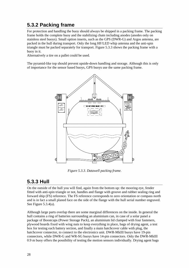
Packing frame 5.3.2For protection and handling the buoy should always be shipped in a packing frame. The packing frame holds the complete buoy and the stabilizing chain including anodes (anodes only on stainless steel buoys). Small option inserts, such as the GPS (DWR-G) and Argos antenna, are packed in the hull during transport. Only the long HF/LED whip antenna and the anti-spin triangle must be packed separately for transport. Figure 5.3.3 shows the packing frame with a buoy in it. Alternatively a tire on a pallet could be used. The pyramid-like top should prevent upside-down handling and storage. Although this is only of importance for the sensor based buoys, GPS buoys use the same packing frame.

Figure 5.3.3. Datawell packing frame.

Hull 5.3.3On the outside of the hull you will find, again from the bottom up: the mooring eye, fender fitted with anti-spin triangle or not, handles and flange with groove and rubber sealing ring and forward ship (FS) reference. The FS reference corresponds to zero orientation or compass north and is in fact a small planed face on the side of the flange with the hull serial number engraved. See Figure 5.3.4(a). Although large parts overlap there are some marginal differences on the inside. In general the hull contains a ring of batteries surrounding an aluminium can, in case of a solar panel a package of Boostcaps (Power Storage Pack), an aluminium lid clamped with four fasteners, plywood boards fixed with wing nuts to keep everything in place, bags of drying agent, a test box for testing each battery section, and finally a main hatchcover cable with plug, the hatchcover connector, to connect to the electronics unit. DWR-MkIII buoys have 19-pin connectors, while DWR-G and WR-SG buoys have 14-pin connectors. Only the DWR-MkIII 0.9 m buoy offers the possibility of testing the motion sensors individually. Drying agent bags

29

are fixed with Velcro straps; see Figure 5.3.4(b). In case of a DWR-G 0.4 m buoy, the hull merely contains 4 batteries. Drying agent bags and a step-up converter with power plug and battery test point are fixed on the plywood.

Figure 5.3.4. Rendering of the hull components, 0.9 m diameter. (a) shows the exterior and (b) the interior.

30

Figure 5.3.5. Contents of the aluminium can in case of (a) a WR-SG and (b) a DWR-MkIII

So far the contents of the aluminium can has not been described. In the DWR-MkIII and WR-SG 0.9 m and 0.7 m diameter, Figure 5.3.5 the can houses the motion sensor package and water temperature sensor at the bottom and partly inside the mooring eye. The motion sensor package consists of electronics boards, a stabilized platform with vertical accelerometer, pitch-roll sensors, two horizontal accelerometers and a three-axial fluxgate compass.

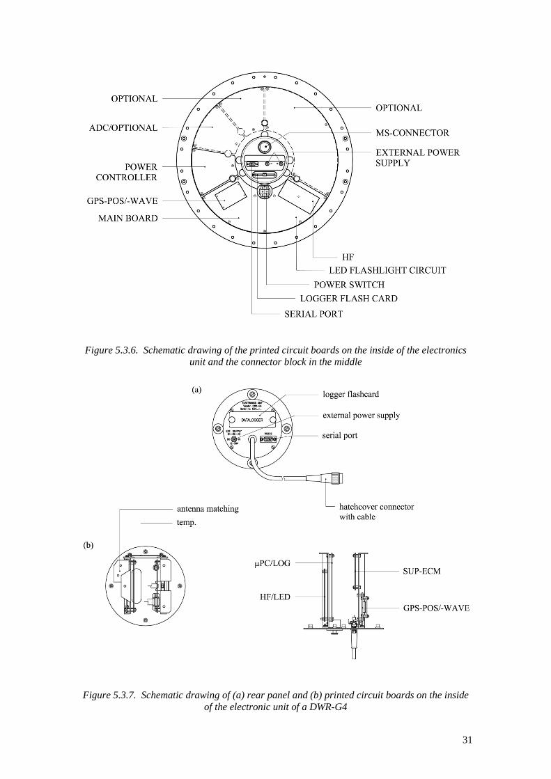
Electronics unit 5.3.4The electronics unit has been designed from the point of view of modularity. A range of printed circuit boards each with its own functionality and its own location will fit in the unit. Figure 5.3.6 and 5.3.7 (b) schematically shows the location of the boards; the interconnecting ribbon cables and coaxial cables are not shown. For a more detailed description of the printed circuit boards and their functionality see chapter 5.11.2.

31

Figure 5.3.6. Schematic drawing of the printed circuit boards on the inside of the electronics unit and the connector block in the middle

Figure 5.3.7. Schematic drawing of (a) rear panel and (b) printed circuit boards on the inside of the electronic unit of a DWR-G4

32

Hatchcover 5.3.5Two hatchcover versions exist: one with two and one with three ports. These ports are designated HF (whip antenna with LED flasher), GPS (GPS antenna for GPS position on DWR-MkIII and WR-SG and GPS wave measurement on DWR-G alike) and, in case of three ports, the third port is designated to Argos, Iridium or GSM, consistent with prefixed cabling below. All ports require a rubber sealing ring for waterproof sealing. The ports are centred on the hatchcover leaving enough separation to avoid contact and interference between the antennae, Figure 5.3.8. To close the hatch 24 hexagon socket screws are used and the applied torque should be approximately 10 Nm. The hatchcover can be lifted by using the threaded hole and one of the screws, in case of under pressure. See Figure 5.3.9. Due to its smaller size the 0.4 m GPS buoy does not have ports, but rather a fixed set of antennas. It is fastened with 8 hexagon socket screws (no threaded hole).

Figure 5.3.8. Drawing of the hatchcover components, (a) top side and (b) bottom side.

33

Figure 5.3.9. Opening the hatchcover by using a screw in the lifting hole.

Antennae 5.3.6The antennae are also part of the modular design of the DWR-MkIII, DWR-G and WR-SG. Not only will it be possible to replace antennae with upgraded versions, but you may also extend buoy functionality with future options that are not even perceived yet. Figure 5.3.10 shows the antennae that are currently available. Mounting an antenna on a port is straightforward. Make sure antenna and port are clean and dry. Check if the rubber sealing ring is in place and lower the insert in the port, allowing the connectors to centre. A slight tolerance on the antenna connector will accommodate small misalignment. The connector inside the port is waterproof. This means that water will not enter the buoy if your antenna is leaking (after a collision or if the rubber sealing ring is absent). Nevertheless, electrical short-circuits may stop the buoy from functioning. Blind covers are available to cover unused ports. Use the 6 hexagon socket screws to fasten the antenna, see Figure 5.3.11. The port labelled GPS is intended for a GPS position antenna, for DWR-MkIII and WR-SG buoys, or a GPS wave antenna, for DWR-G buoys. In the case of the GPS wave antenna, the antenna is placed on an identical spring in order to overlook the HF antenna spring and the buoy sides when the buoy is tilted. GPS positioning is less demanding, therefore the GPS antenna will be placed directly on the flange of the port without a spring. Argos, Iridium and the GSM antenna will be mounted on the unlabelled option port (see Figure 5.3.8). The modular design of the electronics unit and the ports on the hatchcover already provides for these options and allows easy upgrading of your wave measurement equipment. Due to lack of space the DWR-G 0.4 m does not feature option and mounting ports, instead a GPS antenna, LED flasher and HF whip antenna base are mounted permanently. Visit our website or subscribe to our semi-annual bulletin e-mailing if you want to be informed when new options become available.

34

Figure 5.3.10. Different types of antennae: CAT4/HF whip including LED flasher(a), HF whip including LED flasher(b), LED flasher only whip(c), GPS wave(d), GPS position(yellow)(e),

Argos(f) Iridium(black)(g), GSM(h).

Figure 5.3.11. Illustration of how to fix an antenna or sensor option

to a port. Please make sure the rubber sealing ring is in place.

35

5.4 Wave motion sensors: Accelerometers, inclinometers and compass Wave height, principle of measurement 5.4.1

The DWR-MkIII and WR-SG measure wave height by means of a single accelerometer. The sensitive axis of this accelerometer points in the vertical direction. After filtering and double integration of the acceleration signal the motion of the buoy, hence the wave motion is obtained. The strength of the Datawell principle is its gravity-stabilized platform. This patented principle is unique and we will come to the advantages below. Essentially, the platform is formed by a suspended disk in a fluid of equal density. By means of a very small metal weight the disk is made gravity sensitive. The large mass of the fluid in combination with the small force of the metal makes a pendulum with a natural period of 40 s, corresponding to a pendulum length of 400 m. This platform remains almost horizontal under any movement which can be expected at sea. Mounting the accelerometer on this stabilized platform makes the measurement of wave height through vertical acceleration straightforward.

Wave direction, principle of measurement 5.4.2Wave direction is determined by measurement of the horizontal motion of the buoy and correlating this motion with the vertical motion of the buoy. Two mutually perpendicular accelerometers are mounted in the DWR-MkIII which measure the horizontal buoy motion in case the buoy is in the upright position. In case of tilt, the pitch and roll angles are determined by coils around the sensor sensing the electromagnetic coupling with a coil on the stabilized platform. With the help of the pitch and roll sensors the measurements of the above mentioned acceleration sensors are transferred to real horizontal acceleration. With the help of a fluxgate compass the acceleration in buoy-coordinates is transferred to north-west-coordinates. The beauty of the Datawell principle is that it has kept the vertical acceleration out of all the transformations, thus ensuring that you get the best wave heights possible.

Buoy axes and references 5.4.3The DWR-MkIII motion sensor package measures 8 observables: 3 accelerations Ax, Ay, Av, 3 magnetic field strengths Hx, Hy Hz, and pitch and roll. Figure 5.4.1 defines the directions of x, y, z and vertical axes. All directions are referenced to the hull serial number plane (y) and normal (x), the axis of rotation (z) fixed to the buoy and the vertical axis (v) determined by the force of gravity. Suppose you were facing the hull serial number. Tilting the buoy towards you would result a positive pitch and a negative x-acceleration or Ax output. Note that an accelerometer sensor actually is a force sensor and that with a tilted buoy the force of gravity will act as an inertial force. If you add that the direction of acceleration is opposite to the direction of the inertial force or gravity force, you will understand why Ax is negative. Similarly, tilting the buoy towards the left would result a positive roll and a positive y-acceleration or Ay output. Considering an upright buoy, if the positive Ax direction would point towards the north then the positive Ay direction would point westward and the positive z-axis would be directed upward. Double integration would yield north, west and vertical motion. The signs of the compass outputs correspond to the positive x-, y-, but negative z-direction. Directing the serial number towards the north will yield a positive H x and zero orientation. Looking from above a right angle clockwise rotation yields +90º orientation and a positive Hy. Note that the Hz-axis is fixed to the hull whereas the Av-axis always points up and is fixed to the stabilized platform.

36

For a tilted buoy the orientation is the same as for an upright buoy, which may be verified by tilting the buoy.

Figure 5.4.1. Definition of the axes and signs of the DWR-MkIII motion sensors.

Inspection of the fluid level 5.4.4As mentioned in Chapter 2 Maintenance it is important for the stabilized platform and vertical accelerometer sensor to periodically check the fluid level within the plastic sphere. The fluid level can be visually inspected through the Perspex lid on the sphere, see Figure 5.4.2. If the centre of the rubber membrane is pointing upwards, Figure 5.4.2(b), the fluid level is sufficient. In case the membrane touches the Nylon screw, Figure 5.4.2(a), the fluid is too low and fluid has to be added. Datawell advises to check the fluid level every 3 years. Based on experience the sensor requires a small refill after 3 to 6 years. Only fill up the sensor in a clean environment to avoid contamination of the fluid. Do not insert anything but the original sensor fluid. Datawell will readily supply you with a small amount. To avoid damage by spilled fluid wrap some tissue paper around the neck of the sensor. Take off the plastic lid by unscrewing the 6 screw-bolts. Remove the rubber membrane and pour some fluid into the sensor until the level is about 1.5 cm below the top. Reposition the rubber membrane without trapping air beneath it. Some deformation of the membrane may be necessary to do so. Fasten the plastic lid again with the 6 screw-bolts. Remove the tissue and wipe away all spilled fluid on the outside of the sensor.

37

Figure 5.4.2. Examples of the fluid level of the stabilized platform and vertical accelerometer sensor: (a) fluid level too low, (b) fluid level sufficient.

Sensor fluid and temperature 5.4.5It has been written repeatedly that the accelerometer based buoy must not be stored below temperatures of −5 ºC. This is determined by the freezing temperature of the fluid surrounding the stabilized platform. While the buoy is deployed at sea, the temperature of the sensor fluid Ts mainly depends on the water temperature Tw and to a certain extent on the air temperature Ta, approximately as

)(1.0 waws TTTT −+= (5.4.1) This will limit the use of the buoy near the north and south poles. In practice, it may be inevitable to expose the buoy to temperatures lower than −5 ºC. On a short time scale this is acceptable as long as you consider the following. The time constant τ of heat transfer from the sensor to the outside is about τ = 70 hrs. Starting from the initial temperature of the sensor Tso and the air temperature Ta to which the buoy will be exposed, the time it will take to cool down the sensor fluid to −5 ºC may be calculated

−−

−=−

ao

asoC TC

TTt o

5ln5 t (5.4.2)

All temperatures are in degrees Celsius. As long as the exposure time remains below the maximum of t−5 ºC the exposure to the low temperature is acceptable.

38

Calibration of the vertical accelerometer 5.4.6A calibrated vertical accelerometer and stabilized platform should perform within limits over 6 years, depending on operating conditions. Consequently Datawell recommends recalibration of your buoy every 6 years. To eliminate any doubt about the calibration, the following tests may be carried out. To test the vertical accelerometer, the buoy must be set in motion first. With a weight of over 200 Kg, a buoy in motion must be approached with great caution! There are two easy ways to obtain a vertical motion:

(1) set a suspended buoy swinging (2) use the rubber cords to set the buoy oscillating vertically (not WR-SG 0.7 m)

The measured vertical motion can be monitored using the buoy receiver and wave software. For the swing use a rope of 10 m and set the buoy swinging with 1 m horizontal amplitude. Maintain the amplitude by gently pushing the buoy each cycle. A heave oscillation with roughly 6 s period and 2.5 cm amplitude should result. When testing with the rubber cords, the procedure is as follows. Fold the 30 m rubber cord twice or (each of) the 15 m rubber cords once, to construct a 7.5 m pendulum, excluding 4-6 m. elongation of the rubber cord under the weight of the buoy. The expected elongation of 10 m explains why this test is not suitable for WR-SG 0.7 m. Attach the lower end of the complete string of rubber cords to a long rope tied to both buoy handles. The upper end of the complete string must be attached overhead. An elastic system with a natural period of vertical oscillation of around 4 seconds will result. Amplitudes of about 2 m are obtainable. Hoist the buoy to a height that a standing man can just reach the mooring eye. The oscillation amplitude will be approximately equal to the height of the mooring eye over the ground. Draw the buoy down until the mooring eye touches the ground and let go. The buoy should be kept oscillating in a way so that the eye just touches the ground by pushing down gently each time the buoy comes down. On hard ground, place a soft pad to avoid bumping. For exact calibration of the heave the buoy must be sent back to Datawell Service.

Platform offset and stability 5.4.7Here two tests are described that focus on the stabilized platform, more precisely its offset and stability. Let us start with testing the offset. Place your buoy upright on a revolving frame or trolley. Take measures to log both pitch and roll signals; consult subsection 5.9.9 on the intelligent test box. Rotate the frame or trolley 1.5 times 360º around the vertical axis and start logging for 0.5-1 hour. Now plot the logged pitch and roll against each other and skip the first 1.5 minute or so. A circle should be written over a time lapse of approximately 30 minutes. The radius of this circle represents the platform offset. It should stay below 1º. To test the stability, leave the buoy at rest on a trolley for a while. Then start logging the buoy motion. Push and stop the buoy fiercely thus moving it a few metres. In particular, the horizontal displacements will show disturbances at the natural swinging period of 40 s of the stabilized platform. If large disturbances occur at all kinds of frequencies, the platform has become unstable. For example, this could be due to a separation of the sensor fluid after cooling down to below −5 ºC. Contact Datawell Service for repair.

39

Magnetic compass 5.4.8The fluxgate compass measures the components of the earth magnetic field in three perpendicular directions referenced to the buoy frame: x-, y- and z-axis. The compass consists of an aluminium cube with three holes in three mutually perpendicular directions. In each hole a magnetic field sensor is placed. This part requires extremely little service. Before any checks can be carried out we must make sure that the local magnetic field is stable and homogeneous. This is not a simple matter in many indoor situations with large DC currents present or near iron structures. Two compass related outputs may be easily obtained through the console: the orientation of the buoy and the local inclination of the earth magnetic field. Use the status request command. By rotating the buoy over 90º or 180º angles the orientation angle can be checked. A correct (within a few degrees) inclination angle indicates that: (1) the platform offset is small and (2) the compass is functioning well. For optimum measurements the stabilized platform should be allowed some 20 min to come to rest. The inclination angle test should reproduce the same value when rotating or tilting the buoy. Such behaviour in fact proofs that not only the platform offset is all right but also pitch and roll and the three compass axes sensors function properly.

Pitch and roll 5.4.9As described, pitch and roll are measured through magnetic coupling between the pick-up coil on the platform inside the sphere and the respective pair of pick-up coils outside the sphere. Also these sensors hardly require service ever. For verification of pitch and roll calibration the buoy is best put in its packing frame with Forward Ship direction/hull serial number face along one of the 4 sides. A well-defined tilt angle of the packing frame in any of the 4 directions can be realized by placing a piece of wood underneath. Consult the buoy axes subsection for directions and signs. Pitch and roll outputs can be directly measured at the intelligent test box, subsection 5.9.9, using a voltmeter.

Horizontal accelerometers 5.4.10Both fixed x- and y-accelerometers are contained in a small stainless steel can. The can is filled with a similar fluid as the plastic sphere incorporating the stabilized platform. However, evaporation through steel is negligible and checking of the fluid level is superfluous. As for the pitch and roll, the packing frame comes in handy to check the horizontal accelerometers as well. Consult the buoy axes subsection once more and connect a voltmeter over the respective terminals at the intelligent test box.

Filtering 5.4.11The final goal is to measure the waves. Now there are two limitations that will keep the buoy from accurately measuring the waves. At higher frequencies, the wave wavelength becomes comparable to the buoy dimensions and the buoy will not be able to follow the particular waves anymore (geometric attenuation). As higher frequency measurements can only introduce noise, all analog outputs of the DWR-MkIII sensors are filtered by applying a low-pass filter with a cut off frequency of 1.5 Hz. The filtered sensor outputs are then sampled and transformed to north, west and vertical accelerations all at a rate of 3.84 Hz. In case of the WR-SG there is no analog filtering. By using a high sampling rat of 10.24 Hz all filtering can be done digitally. The cut off frequency is 2.0 Hz.

40

Another limitation comes from the sensors themselves. At the low frequency end accelerations become very small and disappear in the sensor noise. Therefore, for the DWR-MkIII, a digital high-pass filter with a cut off at 30 s is applied to the 3.84 Hz samples. At the same time it converts the sample rate to 1.28 Hz. Finally, these accelerations are doubly integrated to give the three-dimensional buoy motion in the frequency range of 0.033-0.64 Hz. Again for the WR-SG the high-pass filter is applied to the 10.24 Hz samples and cuts of at 24 s. Furthermore, the sampling rate is converted to 2.56 Hz. After double integration only vertical buoy motion in the frequency range 0.042-1.0 Hz results.

Specifications 5.4.12For the non-Directional Waverider (WR-SG) see Table 5.4.3 and for the Directional Waverider MkIII (DWR-MkIII) see Table 5.4.4.

Table 5.4.3. Specifications of WR-SG.

Parameter Value Heave Range −20-+20 m Resolution 1 cm Scale accuracy (gain error) < 0.5 % of measured value after calibration

< 1.0 % of measured value after 3 year Zero offset < 0.1 m Period time 1 s-24 s Cross sensitivity < 3% Filter Sampling frequency 10.24 Hz Digital filtering type phase-linear, combined band-pass

and double-integrating FIR filter Filter delay 104.7 s HF Output buffer delay and actual HF output

5.5 s (exact, does not apply to logger files)

Data output rate 2.56 Hz Band-pass characteristics 0.050-0.99 Hz: 0.03 dB

0.048-0.99 Hz: 0.3 dB 0.042-1.0 Hz: 3 dB

Extreme temperatures Operating (in water) −5 ºC-+35 ºC (water temperature) Storage −5 ºC-+40 ºC Short term storage (weeks) max. 55 ºC Short term storage min. see Equation (5.4.2)

41

Table 5.4.4. Specifications of DWR-MkIII. Parameter Value Heave Range −20-+20 m Resolution 1 cm Scale accuracy (gain error) < 0.5 % of measured value after calibration

< 1.0 % of measured value after 3 year Zero offset < 0.1 m Period time 1.6 s-30 s Cross sensitivity < 3% Direction Range 0º-360º Resolution 1.5º Reference magnetic north Buoy heading error 0.4º-2º depending on latitude, typical 0.5º Period time in free floating condition 1.6 s-30 s Period time in moored condition 1.6 s-20 s Filter Sampling frequency 3.84 Hz Digital filtering type phase-linear, combined band-pass

and double-integrating FIR filter Filter delay 133.3 s HF Output buffer delay and actual HF output

5.5 s (exact, does not apply to logger files)

HF Data output rate 1.28 Hz Band-pass characteristics 0.056-0.58 Hz: 0.03 dB

0.04-0.59 Hz: 0.3 dB 0.033-0.6 Hz: 3 dB

Low frequency side 24 dB/octave High frequency side > 60 dB Extreme temperatures Operating (in water) −5 ºC-+35 ºC (water temperature) Storage −5 ºC-+40 ºC Short term storage (weeks) max. 55 ºC Short term storage min. see Equation (5.4.2)

42

5.5 Wave motion sensor: GPS Wave measurement principle 5.5.1

The GPS principle of wave measurement is explained by analogy. Apart from distance measurements between satellite and receiver, the so called GPS code phase, some GPS receivers also provide Doppler measurements. The former are used in GPS positioning, whereas the latter are indicative of satellite and receiver velocities. We exploit the analogy of Doppler frequency shifts for sound waves from moving sources. As for a passing car blowing its horn, it is in principle possible to track the motion of the car by listening to the sound of the horn. The more the frequency differs from the original frequency of the horn source, the higher the speed of the car. Integrating over time then yields the motion of the car.

GPS motion sensor 5.5.2A GPS motion sensor consists of a GPS antenna and a GPS receiver. A patented algorithm will calculate the motion of the antenna centre. The procedure of testing the GPS motion sensor is rather simple. Just leave the DWR-G buoy in a place where it has a clear view of the sky (no buildings or trees) and set it running. If the resulting north, west and vertical signals remain within a few centimetres approximately the sensor is alright. It may seem paradoxical to test a motion sensor by leaving it motionless. The way out of this paradox is that GPS satellites orbit the earth with velocities of 4 Km/s and any motion of the GPS receiver only forms a minor contribution. So if a motionless GPS motion sensor correctly produces a no-motion result in a highly dynamic situation then it works fine.

GPS and atmospheric or marine conditions 5.5.3In line with the military and strategic intentions of the GPS system, GPS receivers and therefore the GPS buoy, will continue functioning during rain, snow or hail storms. The only problematic meteorological situation is when the GPS antenna is covered with a continuous layer of ice. As for marine conditions, spray will also not impede the normal operation of the buoy. However, GPS signals do not penetrate through a continuous layer of salt or fresh water. A breaking wave washing over the GPS antenna will result in data missing. Apart from meteorological and marine influences, also dirt, paint or metal constructions added by the user may block the GPS signal. If the GPS antenna has become dirty, clean it with water and soap and a soft piece of cloth.

GPS antenna and pseudo-motion 5.5.4To be precise the three-dimensional motion of the GPS antenna is measured and not that of the centre of the buoy. This implies that pitching and rolling of the buoy will result in measured (GPS antenna) ‘wave’ motion, even on a perfectly smooth sea surface. This false motion is addressed as pseudo-motion. Experiments where pitch and roll have been logged, have demonstrated that the Fourier spectrum of the pseudo-vertical always remains far below the wave spectrum. In the case of pseudo-horizontal motion, only on the high frequency side, above 0.5 Hz, the pseudo-spectrum may be comparable to the true wave motion. This is consistent with the fact that pitch and roll will exert a larger effect on the horizontal than on the vertical pseudo-motion component. Furthermore, the frequency given is consistent with the typical pitch and roll behaviour displayed when the floating buoy is tilted by hand and is released.

43

Limit on buoy velocity 5.5.5The processing cannot keep up with position changes over 100 m in less than 100 s and measurements will start to fail. E.g. when a buoy is used free floating or is towed at constant velocities above 1 m/s. This will appear as sudden large oscillations in the displacement data.

Signal loss and flag 5.5.6In the example of the passing car, one will lose track of the car if one temporarily closes one’s ears. Likewise if the GPS receiver temporarily loses signal, due to waves washing over or a momentarily extreme tilt, the buoy velocity is temporarily unknown. As a result the buoy motion may contain discontinuities. However the GPS receiver knows when signal loss occurs and will inform the user of this through setting a flag: the least significant bit of the north. In practice, breaking waves in the surf zone and areas of strong current must be avoided. Wave height by itself is not a problem. In other locations signal loss occurs less than 0.1% of the time.

Selective availability 5.5.7As mentioned the GPS system originally was and still is a military system, maintained by the United States Department of Defence. As such a few features are incorporated to restrict the use of precise GPS to selected users. This is known as Selective Availability (SA). When SA is active a dither is added to the satellite GPS time thereby deteriorating the GPS position accuracy from 10 m to 100 m. Furthermore the precision of the satellite orbit information may be reduced. The information to correct for dithering is encrypted in the GPS signal. Unless one has the encryption key one cannot restore the intrinsic GPS accuracy. On May 1, 2000 SA was officially discontinued, see www.navcen.uscg.gov/gps/selective_availability.htm. If, in the unlikely event, SA would be temporarily switched on for strategic reasons, the current GPS wave buoy will not work anymore! However, it will continue measuring waves immediately after SA is switched off again.

Filtering 5.5.8Measured velocities are digitally filtered using an integrating high-pass filter with a cut-off at 0.01 Hz. Moreover, the intrinsic 2 Hz sampling is converted into 1.28 Hz north, west and vertical motions to fit the long existing transmitter data format. Use is made of a so-called decimation filter, which causes an extra delay.

44

Specifications 5.5.9See Table 5.5.1.

Table 5.5.1. Specifications of DWR-G. Parameter Value Heave, north, west Range −20 m-+20 m Resolution 1 cm Accuracy ±1 cm or 0.1% of value,

whichever is worse Period time (frequency range) 1.6 s-100 s

(0.01 Hz-0.64 Hz) Direction Range 0º-360º Resolution 1.5º Accuracy 1.5º Reference true north (WGS84) Filter Sampling frequency 2.0 Hz Digital filtering type phase-linear, combined band-pass

and single-integrating FIR filter Filter delay 256.0 s Decimation filter delay 43.0 s HF output buffer delay and actual HF output

5.5 s (approximately, does not apply to logger files)

Data output rate 1.28 Hz Band-pass characteristics 0.0154-0.59 Hz: 0.0013 dB

0.0132 0.009 dB 0.0115 0.09 dB 0.01 Hz 0.8 dB low frequency side 52 dB/octave (< 0.01 Hz)

5.6 Data processing Independent of the type of sensor, the DWR-MkIII and DWR-G generate raw north, west and vertical displacements at a rate of 1.28 Hz. The WR-SG however generates vertical displacements at 2.56 Hz. Displacements refer to excursions from the average position and should not be mistaken for position changes relative to the previous position. The raw data is stored on the logger flash card and output through the radio link. However, the buoy also outputs processed data through the radio link or via communication satellite. Processed data are much more compact, nevertheless they still give a good impression of the sea state. Especially for the limited data transmission capacity of satellites, the processing and compressing is essential. The processing method is the topic of this section. In oceanography the use of Fourier spectra of the vertical displacements to represent the wave conditions is wide-spread. The power spectral density PSD thus obtained quickly shows what wave amplitudes occur at what frequencies. The first part of this section is devoted to this straightforward Fourier spectrum calculation and applies to all Waveriders. In the second part we will deal with a more sophisticated Fourier analysis that also incorporates the horizontal motion. Now also information on wave ellipticity, wave direction, direction spread, etc. becomes available. This part only applies to Directional Waveriders (DWR-MKIII, DWR-G).

45

Wave height spectrum 5.6.1In the directional buoys (DWR-MkIII, DWR-G), the internal wave spectrum is calculated as follows. At a sampling rate of fs = 1.28 Hz, every 200 seconds a total number of N=256 heave samples hk are collected hk = h(kDt), k=0..N-1 (5.6.1) where Dt=1/fs is the sampling time. A fast Fourier-transform (FFT) is applied to obtain a spectrum in the frequency range 0 to fs/2 = 0.64 Hz, having a resolution of fs/N = 0.005 Hz. The FFT yields Fouriercoefficients according to:

∑−

=

−=∆===1

0

10/)/2exp()(N

klkkll NltNlfNklihwfHH 2π (5.6.2)

with i = √(−1). The wk indicate the window coefficients. Datawell applies a cosine-shaped window over the first and last 32 samples, according to

31032

cos121

255 2=

−== − kkww kkπ (5.6.3a)

1=kw otherwise (5.6.3b) For normalization all window coefficients must be divided by

∑−

=

=1

0

2N

kksnorm wfw (5.6.4)

The power spectral density is obtained from the Fourier coefficients 2

00 )( HfPSD = (5.6.5a)

12/1)( 22 −=+= − NlHHfPSD lNll 2 (5.6.5b)

22/2/ )( NN HfPSD = (5.6.5c)

where frequencies range from 0.0 Hz to 0.64 Hz in steps of 0.005 Hz. Actually, there is one more step, all coefficients are smoothed according to

11 41

21

41

+− ++= llll PSDPSDPSDPSD (5.6.6)

To limit the number of frequencies low frequency coefficients (fl ≤ 0.1 Hz) are left as they are, while only every other smoothed coefficient on the high frequency side(fl > 0.1 Hz) is kept in the spectrum file. Finally, 8 consecutive spectra covering 1600 s are averaged and used to compute the half-hourly wave spectrum. Each half-integral hour (1800 s) a new cycle starts.

Wave direction spectrum 5.6.2So far only the vertical displacements have been processed to give the wave power spectral density. When north and west displacements are included into the processing, much more wave information can be obtained. Starting from the time-series of north, west and vertical (n, w, v) displacements, the three associated Fourier series may be calculated. Each Fourier series consists of a number of Fourier coefficients, which in turn consist of a real and imaginary part.

46

Thus six Fourier components per frequency f are obtained αnf, βnf, αwf , βwf , αvf and βvf or in vector notation: nfnfnf iA βα += (5.6.7a) wfwfwf iA βα += (5.6.7b) vfvfvf iA βα += (5.6.7c) Building on this, co- (C) and quadrature-spectra or quad-spectra (Q) may be formed, e.g. (we shall omit the frequency subscript hereafter) wfnfwfnfwfnfnw AAC ββαα +=⋅= (5.6.8) nfvfnfvfnfvfvn AAQ αββα −=×= (5.6.9) In total 9 components arranged in a 3x3 matrix will be obtained for both co- and quad-spectra. However, not all components need to be calculated. By definition we have 0=== vvwwnn QQQ (5.6.10) Furthermore, Q represents rotation. To give an example, a wave rolling eastward will have a rotation component directed to the north (right-handed screw) and hence Qvw ≠ 0 and Qwv ≠ 0. The rotation in the waves is particularly clear for breaking waves in the surf zone. A rotation component directed vertically would represent eddy currents which are not part of the physics of waves, therefore we also have 0== nwwn QQ (5.6.11) Thus, one obtains:

vvvnvw

nvnnnw

wvwnww

CCCCCCCCC

(5.6.12)

and

00000

vnvw

nv

wv

QQQQ

(5.6.13)

Given these components a whole set of informative wave parameters such as: wave direction, direction spread, wave ellipticity can be obtained. Before discussing their meaning in more detail, first, all formulas will be given.

( ) vvwwnn

nv

CCCQ

a+

=1 (5.6.14)

47

( ) vvwwnn

wv

CCCQ

b+

−=1 (5.6.15)

wwnn

wwnn

CCCC

a+−

=2 (5.6.16)

wwnn

nw

CCC

b+

−=

22 (5.6.17)

These are the first four Fourier coefficients of the normalized directional distribution ),( fG θ

+++++= ...2sin2cossincos

211),( 2211 θθθθ

πθ babafG (5.6.18)

alternatively cast as

+−+−+−+= ...)(2sin)(2cos)cos(

211),( 020201 θθθθθθ

πθ nmmfG (5.6.19)

where ),arctan( 110 ab=θ (5.6.20)

21

211 bam += (5.6.21)

02022 2sin2cos θθ bam += (5.6.22) 02022 2cos2sin θθ ban +−= (5.6.23) The m- and n- coefficients are known as the centred Fourier coefficients [Kuik88] or the second harmonic of the directional energy distribution recalculated to the mean wave direction. Wave direction ),(arctan0 nvwv QQD −== θ (5.6.24) Directional spread 122 mS −= (5.6.25) Wave ellipticity or 1/K where K is the check factor

wwnn

vv

CCC

K+

== /1ε (5.6.26)

Power Spectral Density vvCPSD = (5.6.27)

48

In the present context parameters ai and bi are just helpful intermediate variables. In terms of this more intricate Fourier analysis we again arrive at the power spectral density. Its value and meaning already have been mentioned. Wave ellipticity indicates the shape of the wave. For wavelengths much smaller than the depth, waves describe circular orbits and the ellipticity is near 1. However, if the wavelength becomes comparable to or larger than the depth, the vertical displacements are smaller than the horizontal ones and the ellipticity is smaller than 1. The variation of the ellipticity with wave frequency is indicative of the local depth. Historically, Datawell refers to its reciprocal as check factor. When testing the buoy in a Ferris wheel the ‘wave ellipticity’ should yield 1 of course. In the case of stabilized platform accelerometer-based motion sensors, however, the ellipticity is seen to deviate by a small factor at the lower frequencies. This serves as a check on platform stability and the parameter, the reciprocal of the wave ellipticity is named accordingly. Wave direction and spread speak for themselves. By a close look at the simultaneous north and west motion the wave direction can be determined. For clarity the Datawell wave direction is the direction from which the waves arrive. Both are expressed in radians. In this analysis we have followed the analysis in [Long63].

5.7 Data format Datawell uses two types of message formats: the real-time format and the message format. The Datawell real-time format refers to the long-existing hexadecimal vectors with vertical, north and west displacements and words ultimately forming the spectrum and system files. It is mainly used for relatively low-speed, continuous, near real-time data transmission over the standard HF radio link. More recently, the Datawell message format has been introduced. This format has been prompted by an ever increasing number of datalinks and sensors. It is more suited to data bursts over relatively high-speed links or expensive links. The message format is independent of the link, easy to extend and easy to process in software.

Datawell real-time format 5.7.1The real-time format is organized at four levels

(1) Vectors of 64 bits with real-time data together with cyclical data (2) Blocks of 18 vectors assembling cyclical data with spectral and system data (3) Spectral data of 16 blocks complete a spectrum file (4) System data of 16 blocks complete a system file

More precisely one or two samples of the real-time data are framed in one 64-bit vector, but the 64-bit vectors also contain fractions of cyclical data. After collecting 18 vectors all fractions of cyclical data form a complete block of cyclical data. Similarly, one cyclical data block contains a fraction of a complete spectrum and system file, which require 16 blocks or 288 vectors to assemble. The full set of cyclical data in 16 blocks makes up a system file and a spectrum file. Below all four levels are explained in detail. Timing and the derived compressed spectrum are also discussed in the following subsubsections.

5.7.1.1 Real-time displacements Each 64-bit vector is subdivided into three parts • cyclical data (sync word or system file word or spectral data words) • real-time displacements (one vertical, north and west sample or two vertical samples) • parity bits for transmission error detection and correction

49

The parity bit algorithm uses a Galois code table to encode 63 bits of a vector. In the receiver these bits are processed to check data integrity and correct for transmission errors. All displacements are given as 12 bit signed integers in cm. The most significant bit (MSB) is the sign bit, MSB = 1 means negative. Table 5.7.1 shows the organization of the 64-bit vector. On DWR-G buoys the least significant bit (LSB) of the north is used as a GPS flag (0 = ok, 1 = error).

Table 5.7.1. Organization of real-time displacements in 64-bit vector. Cyclic data Real-time displacements (1 cm/bit)* Parity bits

WR-SG vertical (even sample) vertical (odd sample) dummy (-628 cm, 101010101010)

see text

DWR-MkIII DWR-G

vertical north** west see text

16 bits 12 bits 12 bits 12 bits 12 bits Bits 63-48 bits 47-36 bits 35-24 bits 23-12 bits 11-0

*MSB is sign, 1 means negative **LSB is GPS flag (DWR-G only)

5.7.1.2 Spectrum file or full wave spectrum One level further up the cyclic data contained within 18 vectors forms one block. The cyclical data is organized as shown in Table 5.7.2. One block provides information on spectral parameters at 4 frequencies. The parameters are: • frequency f • relative power spectral density RPSD • K check factor (reciprocal of the wave ellipticity) • mean direction from D • direction spread S • centred Fourier coefficients (m2 and n2), see Equations (5.6.22) and (5.6.23).

Table 5.7.2. Organization of cyclic data in a block of 18 vectors.

16 blocks constitute a spectrum file or full wave spectrum. The vector number on the left is not transmitted.

No Cyclic data word (16 bits) 1 sync word (hex 7FFF) 2 system file word number

4 bits system file word 12 bits

3 SLSB(n) 2 bits

frequency index n 6 bits

direction D(n) 8 bits

4 M2LSB(n) 2 bits

N2LSB(n) 2 bits

rel. power spectral density RPSD(n) 12 bits

5 spread S(n) 8 bits

M2(n) 8 bits

6 N2(n) 8 bits

check factor K(n) 8 bits

7-10 n+1, same as n 11-14 n+2, same as n 15-18 n+3, same as n

The sync word is repeated every 18 vectors. Its pattern is not likely found elsewhere. SLSB, M2LSB and N2LSB represent the two LSB’s of spread, M2 and N2, respectively. For non-directional buoys (WR-SG) the check factor, direction, spread and centred Fourier coefficients

50

are not meaningful. 16 blocks of 16 vectors (omitting the sync word and system file word number and the system file word itself) make up a complete spectrum file or a full wave spectrum ranging over 64 frequency values. However, the spectral parameters in the cyclic data must be transformed first. Table 5.7.3 explains how the various cyclic data fields translate to the respective spectral parameters. The intermediate point of n = 15 is an exception with a frequency interval running from 0.0975 to 0.105 Hz and with a Δf of 0.0075 Hz.

Table 5.7.3. Translation equations for spectral parameters in spectrum file.

Parameter Equation Remarks Frequency fn = 0.025 Hz + nΔf

fn = 0.11 Hz + (n−16)Δf Δf = 0.005 Hz, n = 0…15 Δf = 0.01 Hz, n = 16…63

Direction D = D 360º/256 0º = north, 90º = east Relative power spectral density

RPSD = exp(−RPSD/200) max 1, multiply by power density in system file

Spread S = 0.4476 (S + SLSB/4) degrees m2 m2 = (M2 + M2LSB/4−128)/128 centred Fourier coefficient (cosine) n2 n2 = (N2 + N2LSB/4−128)/128 centred Fourier coefficient (sine) Check factor (reciprocal wave ellipticity)

K = K/100 K = 1/ε, K = 1 for waves in deep water

5.7.1.3 System file All system file words of 16 blocks are combined into one system file. A complete system file consists of 16 words from 16 consecutive blocks. It takes 16×18 = 288 vectors to acquire one system file. Table 5.7.5 (next page) shows the significance of the system file data. Bits in the 12-bits word are numbered 0 through 11 with bit 11 MSB and bit 0 LSB. LSB and MSB subscripts of Long, Lat and Inc mean least/most significant bits.

5.7.1.4 Timing During half an hour 8 spectra of a 200 s data interval each are collected and averaged. At the end of the half-hour over which the calculations are executed, all (directional) spectral parameters are available. The transmission of one spectrum file takes 225 s. During the next half hour the spectrum file is transmitted 8 times for redundancy. Table 5.7.4 gives an overview of the timing of vectors, blocks and files.

Table 5.7.4. Timing at all levels of data. Unit Size Time Vector 64 bits 0.78125 s (1/1.28 Hz) Block 18 vectors 14.0625 s File 16 blocks (288 vectors) 225 s Full cycle 8 repeated files 30 min

Table 5.7.5a describes the organization of the system file in case no CAT4 option is installed. Table 5.7.5b describes the organization of the system file in case the CAT4 option is installed. The system file is updated every half hour and the most recent information is transmitted at xx:00 and xx:30.

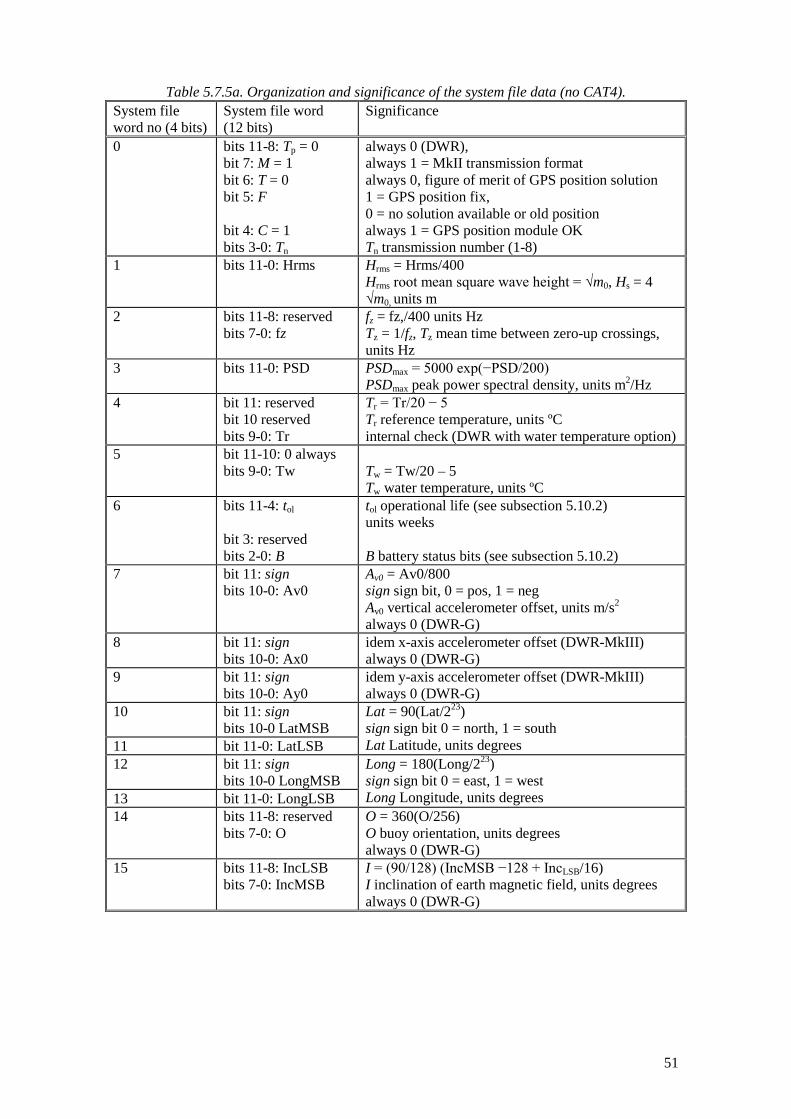
51

Table 5.7.5a. Organization and significance of the system file data (no CAT4). System file word no (4 bits)

System file word (12 bits)

Significance

0 bits 11-8: Tp = 0 bit 7: M = 1 bit 6: T = 0 bit 5: F bit 4: C = 1 bits 3-0: Tn

always 0 (DWR), always 1 = MkII transmission format always 0, figure of merit of GPS position solution 1 = GPS position fix, 0 = no solution available or old position always 1 = GPS position module OK Tn transmission number (1-8)

1 bits 11-0: Hrms Hrms = Hrms/400 Hrms root mean square wave height = √m0, Hs = 4 √m0, units m

2 bits 11-8: reserved bits 7-0: fz

fz = fz,/400 units Hz Tz = 1/fz, Tz mean time between zero-up crossings, units Hz

3 bits 11-0: PSD PSDmax = 5000 exp(−PSD/200) PSDmax peak power spectral density, units m2/Hz

4 bit 11: reserved bit 10 reserved bits 9-0: Tr

Tr = Tr/20 − 5 Tr reference temperature, units ºC internal check (DWR with water temperature option)

5 bit 11-10: 0 always bits 9-0: Tw

Tw = Tw/20 – 5 Tw water temperature, units ºC

6 bits 11-4: tol bit 3: reserved bits 2-0: B

tol operational life (see subsection 5.10.2) units weeks B battery status bits (see subsection 5.10.2)

7 bit 11: sign bits 10-0: Av0

Av0 = Av0/800

sign sign bit, 0 = pos, 1 = neg Av0 vertical accelerometer offset, units m/s2 always 0 (DWR-G)

8 bit 11: sign bits 10-0: Ax0

idem x-axis accelerometer offset (DWR-MkIII) always 0 (DWR-G)

9 bit 11: sign bits 10-0: Ay0

idem y-axis accelerometer offset (DWR-MkIII) always 0 (DWR-G)

10 bit 11: sign bits 10-0 LatMSB

Lat = 90(Lat/223) sign sign bit 0 = north, 1 = south Lat Latitude, units degrees 11 bit 11-0: LatLSB

12 bit 11: sign bits 10-0 LongMSB

Long = 180(Long/223) sign sign bit 0 = east, 1 = west Long Longitude, units degrees 13 bit 11-0: LongLSB

14 bits 11-8: reserved bits 7-0: O

O = 360(O/256) O buoy orientation, units degrees always 0 (DWR-G)

15 bits 11-8: IncLSB bits 7-0: IncMSB

I = (90/128) (IncMSB −128 + IncLSB/16) I inclination of earth magnetic field, units degrees always 0 (DWR-G)

52

*only on DWR-MkIII, reserved on DWR-G

Table 5.7.5b. Organization and significance of the system file data (with CAT4). System file word no (4 bits)

System file word (12 bits)

Significance

4 bit 11: S-flag bit 10: V-flag bits 9-0: Tair

Solar induced uncertainty, S = 0 means no uncertainty, S = 1 means there is solar induced uncertainty. Evaporation detected flag, V = 0 mean no evaporation detected, V = 1 means that evaporation was detected. Tair = Tair/10 − 35 Tair air temperature, units ºC

5 bit 11: 0 always bit 10: 1 always bits 9-0: Tw

Bit 1 indicates CAT4 option is present. Tw = Tw/20 – 5 Tw water temperature, units ºC

5.7.1.5 Compressed wave spectrum The wave spectrum computed internally by the buoy covers 128 frequency bands and is condensed to 64 frequency bands occupying 512 bytes (spectrum file, full wave spectrum). To save bits while maintaining a large range of values an exponential representation of numbers is used. Furthermore, the initial 64 frequency bands of the full spectrum are reduced to 13 bands. Finally, a fixed distribution of the power spectral density (PSD) in a fixed number of frequency bands is predefined. This does away with transmission of the normalized or relative PSD. Only the frequency band limits or band widths need to be transmitted. The compressed wave spectrum consists of 16 words of 16 bits and is detailed in Table 5.7.6. Values must be transformed according to Table 5.7.7.

Table 5.7.6. Compressed wave spectrum data format Word number

Compressed wave spectrum word

Fraction of total variance or integrated PSD

Significance

0 bits 15-13 bits 12-7 bits 6-0

1/512

battery status number frequency upper limit of first band F (lower limit is 0.025 Hz) total variance or integrated PSD M0

1 bits 15-10 bits 9-4 bits 3-0

1/256 frequency band width of next band ΔF direction from D directional spread S

2 1/128 see word 1 3 1/64 see word 1 4 1/32 see word 1 5 1/16 see word 1 6-11 1/8 see word 1 12 1/16 see word 1 13 1/32 see word 1 14 bits 15-10

bits 9-4 bit 3 bits 2-0

17/512 direction from D for remaining band (from upper limit of previous band to 0.635 Hz) mean time between zero up-crossings Tz reserved absolute vertical acceleration offset units 0.32 m/s2 *

15 bits 15-13 bits 12-10 bits 9-0

idem absolute x-acceleration offset* idem absolute y-acceleration offset* water temperature

53

Table 5.7.7 gives the formulas to restore the original parameters from the compressed representation in the 32 byte message. The 32 bytes are organized as 16 words with the most significant byte first.

Table 5.7.7. Compressed wave spectrum back-transformation equations. Parameter Formula Unit Remarks Total variance m0 (integrated PSD)

−

= 1

320exp16.00

Mm m range 8.3 m

min. res. 0.51 cm rel. res. 3.2%

Frequency upper limit f 025.01

32exp04.0 +

−

=

Ff Hz

Frequency band width Δf

−

∆=∆ 1

32exp04.0 Ff

Hz min. 0.00127 Hz max. 0.247 Hz

Mean direction from D )64/(360 DD °= º res. 5.625º (0º = north, 90º east)

Directional spread S

−

= 1

8exp25.0 SS

rad range 1.38 rad (79º) min. 0.033 rad (1.9º) rel. res. 15%

Mean time between zero-up crossings Tz

−

= 1

64exp/125.3 TzTz

s

Water temperature 520/ −=TwTw °C Air temperature 𝑇𝑇air = T 10 − 35⁄ °C

Datawell message format 5.7.2As any message-type format the Datawell message format brings about a high degree of flexibility. In addition, the Datawell message format incorporates two compression methods:

• transformation of real numbers to integers, and • smart decimation

As a result also compact messages for low-capacity, high-cost datalinks such as satellite communication are possible. This subsection starts with the format, listing and discussion of the currently defined messages. After that the abovementioned compression methods are explained.

5.7.2.1 Message format and defined messages Table 5.7.8 describes the general format for the first 15 messages.

Table 5.7.8. Format of the first 15 messages Byte HiNibble LoNibble

0 MsgID (0..9A..E) CRC-4 checksum

1 Data 2 Data … … n-1 Data

For the next 256 messages, the format is described in Table 5.7.9.

54

Table 5.7.9. Format of the 256 messages following the first 15. Byte HiNibble LoNibble

0 Header (F = 1111) CRC-4 checksum

1 MsgID (00..FF)

2 Data … … n-1 Data

The calculation of the CRC-4 checksum is explained in the next subsubsection. Until now, six messages have been defined, see Table 5.7.10. Keeping in mind the due long Argos ID’s, which leaves only 31 bytes for the message body, the size of several messages is limited to 31 bytes. Note that also the combination of messages 3, 5 and 6 totals 31 bytes. In the future, new message formats can be added within the present scheme.

Table 5.7.10. Overview of currently defined messages. MsgID Message Message length

(bytes) 0 Compressed heave spectrum 31 3 Spectral parameters 11 5 Buoy information (“System file”) 10 6 Sea surface temperature 10 9 Compressed directional spectrum 31 A Air temperature 10 F (subindexing) -

5.7.2.2 CRC-4 checksum computation The CRC-4 is a cyclic redundancy check, where the 4 indicates the number of bits in the CRC checksum. Every message m can be considered as a string of n bits bj: m = bn−1 b n−2 b n−3 … b1 b0 (5.7.1) where every bj is either 0 or 1. To this message m we add four bits that are zero: m’ = bn−1 b n−2 b n−3 … b1 b0 0 0 0 0 (5.7.2) This bit string can be interpreted as a binary polynomial: m’(x) = b n−1xn+3 + b n−2xn+2 + b n−3xn+1 + … b1x5 + b0x4 (5.7.3) Now the remainder r(x) is determined of m’(x) divided by a special polynomial, the CRC generator, c(x): c(x) = x4 + x + 1 (5.7.4) The polynomial r(x) will have four binary coefficients: r(x) = r3x3 + r2x2 + r1x + r0 (5.7.5) and these are substituted for the zeros at the end of message m’: m” = bn−1 b n−2 b n−3 … b1 b0 r3 r2 r1 r0 (5.7.6)

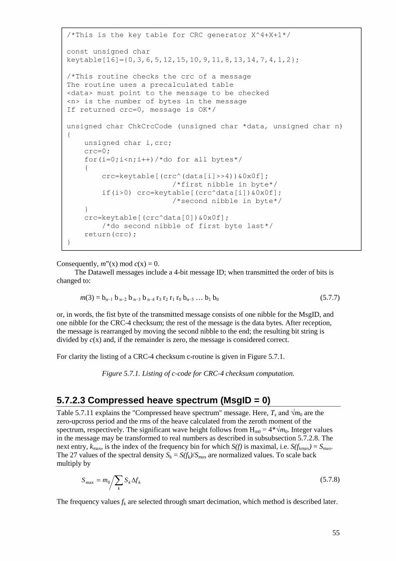
55

Consequently, m”(x) mod c(x) = 0.

The Datawell messages include a 4-bit message ID; when transmitted the order of bits is changed to: m(3) = bn−1 b n−2 b n−3 b n−4 r3 r2 r1 r0 bn−5 … b1 b0 (5.7.7) or, in words, the fist byte of the transmitted message consists of one nibble for the MsgID, and one nibble for the CRC-4 checksum; the rest of the message is the data bytes. After reception, the message is rearranged by moving the second nibble to the end; the resulting bit string is divided by c(x) and, if the remainder is zero, the message is considered correct. For clarity the listing of a CRC-4 checksum c-routine is given in Figure 5.7.1.

Figure 5.7.1. Listing of c-code for CRC-4 checksum computation.

5.7.2.3 Compressed heave spectrum (MsgID = 0) Table 5.7.11 explains the "Compressed heave spectrum" message. Here, Tz and √m0 are the zero-upcross period and the rms of the heave calculated from the zeroth moment of the spectrum, respectively. The significant wave height follows from Hm0 = 4*√m0. Integer values in the message may be transformed to real numbers as described in subsubsection 5.7.2.8. The next entry, kmax, is the index of the frequency bin for which S(f) is maximal, i.e. S(fkmax) = Smax. The 27 values of the spectral density Sk = S(fk)/Smax are normalized values. To scale back multiply by

∑ ∆=k

kk fSmS 0max (5.7.8)

The frequency values fk are selected through smart decimation, which method is described later.

/*This is the key table for CRC generator X^4+X+1*/ const unsigned char keytable[16]={0,3,6,5,12,15,10,9,11,8,13,14,7,4,1,2}; /*This routine checks the crc of a message The routine uses a precalculated table <data> must point to the message to be checked <n> is the number of bytes in the message If returned crc=0, message is OK*/ unsigned char ChkCrcCode (unsigned char *data, unsigned char n) { unsigned char i,crc; crc=0; for(i=0;i<n;i++)/*do for all bytes*/ { crc=keytable[(crc^(data[i]>>4))&0x0f]; /*first nibble in byte*/ if(i>0) crc=keytable[(crc^data[i])&0x0f]; /*second nibble in byte*/ } crc=keytable[(crc^data[0])&0x0f]; /*do second nibble of first byte last*/ return(crc); }

56

Table 5.7.11. Compressed heave spectrum message (MsgID = 0). Byte HiNibble LoNibble

0 MsgID = 0 = 0000 CRC-4 checksum 1 Tz 2 √m0 3 kmax 4 S0 5 S1 … … 30 S26

5.7.2.4 Spectral parameters (MsgID = 3) Table 5.7.12 explains the "Spectral parameters" message. The periods T(n,n+1) := mn/mn+1 and T(n,n+2) := √(mn/mn+2) are computed from the moments mn of the spectrum. ∫= )( fSfdfm n

n (5.7.9)

In addition, Tdw and Goda’s peakedness parameter Qp are included:

)(1 21

0fSfdf

mTdw ∫ −= (5.7.10)

∫= )(2 220

fSfdfm

Qp (5.7.11)

plus the peak period Tp, defined through S(1/Tp) = Smax. See also Table 5.7.17. Other parameters, such as the bandwidth parameters ε and ν, or the significant steepness Ss, can be computed from the periods in the message:

12

1 −

=

zTT

ν (5.7.12)

2

1

−=

z

c

TT

ε (5.7.13)

20 /2 zms gTHS π= (5.7.14)

Table 5.7.12. Spectral parameters message (MsgID = 3).

Byte HiNibble LoNibble 0 MsgID = 3 = 0011 CRC-4 checksum 1 √m0 2 TI = T(−2,0) 3 TE = T(−1,0) 4 T1 = T(0,1) 5 Tz = T(0,2) 6 T3 = T(1,3) 7 Tc = T(2,4) 8 Tdw 9 Tp 10 1/Qp

57

5.7.2.5 Buoy information (system file) (MsgID = 5) Table 5.7.13 explains the "Buoy information" message. The GPS position is a 24-bit Latitude and a 24-bit Longitude. Both are two's-complement values. Positive values are North (East), negative values are South (West). The scaling is: 23

321 2/)1000100000(90 ixixiLat o +⋅+⋅⋅= (5.7.15) 23

654 2/)1000100000(180 ixixiLon o +⋅+⋅⋅= (5.7.16) The battery status is the battery life expectancy, i.e. the number of weeks that the battery cells are expected to last. All three accelerometer offsets are 4-bit numbers, scaled linearly: A = i/8 in units of m/s^2.

Table 5.7.13. Buoy information message (MsgID = 5). Byte HiNibble LoNibble

0 MsgID = 5 = 0101 CRC-4 checksum 1

GPS Latitude

2 3 4

GPS Longitude

5 6 7 Battery Status 8 Av Ax 9 Ay (Reserved)

5.7.2.6 Sea Surface Temperature (MsgID = 6) Table 5.7.14 explains the "Sea Surface Temperature" message. The water temperature Tw is a 10-bit number, scaled linearly: Tw = i/20 −5 in units of °C.

Table 5.7.14. Meteorological parameters message (MsgID = 6). Byte HiNibble LoNibble

0 MsgID = 6 = 0110 CRC-4 checksum 1 Tw 2 Tw

(continued) (Reserved)

3 (Reserved) … … 9 (Reserved)

58

5.7.2.7 Compressed directional spectrum (MsgID = 9) Table 5.7.15 explains the "Compressed directional spectrum" message.

Table 5.7.15. Compressed directional spectrum message (MsgID = 9). Byte HiNibble LoNibble

0 MsgID = 9 = 1001 CRC-4 checksum 1 Dir(peak) 2 Spr(peak) 3 kmax 4 Dir0 5 Dir1-Dir0 Spr1 6 Dir2 7 Dir3-Dir2 Spr3 … … 28 Dir24 29 Dir25-Dir24 Spr25 30 Dir26

Here, Dir and Spr are the mean direction and directional spread. At the top of the table, the direction and spread for the peak in the heave spectrum are given. The peak is defined by kmax in the 3rd row. In the remaining rows, the directional spectrum is specified for the same set of frequencies as the heave spectrum. In the even bins (0, 2, 4, …, 26), the direction is given as a 8-bit integer: *360 / 256=Dir i (5.7.17) which results in a 1.4° accuracy. In the odd bins (1, 3, 5, …, 25), the directional step with respect to the previous direction is given. For these delta-directions ΔDir, a 4 bit two’s-complement is used as explained in Table 5.7.16.

Table 5.7.16. Two's-complement representation of ∆Dir. i ∆Dir i ∆Dir i ∆Dir i ∆Dir 0000 0 0100 +4*360/256 1000 NaN 1100 −4*360/256 0001 +1*360/256 0101 +5*360/256 1001 −7*360/256 1101 −3*360/256 0010 +2*360/256 0110 +6*360/256 1010 −6*360/256 1110 −2*360/256 0011 +3*360/256 0111 +7*360/256 1011 −5*360/256 1111 −1*360/256

The value 1000 is used for labeling a directional step of magnitude greater than 7*360/256 ≈ 10°. In that case, the direction in bin l can be approximated as the mean of the adjacent directions:

1 11 1

1 1 1 1

+ −− +

+ − + −

− −= +

− −l l l l

l l ll l l l

f f f fDir Dir Dirf f f f

(5.7.18)

In the odd bins, the spread is specified as a 4 bit number Sprmax = 78.25, imax = 14, b= 8, see "Transformation of real numbers to integers" below. The even spreads must be constructed from the adjacent spreads:

1 11 1

1 1 1 1

+ −− +

+ − + −

− −= +

− −l l l l

l l ll l l l

f f f fSpr Spr Sprf f f f

(5.7.19)

59

In the first and last bin, the spread is not specified, and interpolation is not possible. Here, extrapolation could be used. However, negative values must be avoided, since these have no physical meaning.

3 0 1 00 1 3

3 1 3 1

− −= −

− −f f f fSpr Spr Sprf f f f

(5.7.20)

26 23 26 2526 25 23

25 23 25 23

− −= −

− −f f f fSpr Spr Sprf f f f

(5.7.21)

5.7.2.8 Air Temperature (MsgID = A) Table 5.7.17 explains the "Air Temperature" message. The water temperature Tw is a 10-bit number, scaled linearly: Tw = i/20 − 5 in units of °C. Its range is -5 to 46.15°C, and its resolution is 0.05°C. The air temperature Tair is a 10-bit number, scaled linearly: Tair = i/10 − 35 in units of °C. Its range is -35 to 67.3°C, and its resolution is 0.1°C.

Table 5.7.17. Air temperature message (MsgID = 0xA). Byte HiNibble LoNibble

0 MsgID = 0xA = 1010 CRC-4 checksum 1 Tw (bits 9..2) 2 Tw (1,0) 0 0 S V Tair (9,8) 3 Tair (7..0) 4 Tw (bits 9..2) 5 Tw (1,0) 0 1 S V Tair (9,8) 6 Tair (7..0) 7 Tw (bits 9..2) 8 Tw (1,0) 0 1 S V Tair (9,8) 9 Tair (7..0)

The message contains three sets of water temperature and air temperature. The first set in bytes 1-3 was measured 30 minutes before the message was transmitted. The second set in bytes 4-6 was measured 20 minutes before transmission. The third set in bytes 7-9 was measured 10 minutes before transmission. The S bit is the solar induced uncertainty flag: S = 0 means there is no uncertainty, S = 1 means there is a solar induced uncertainty. The V bit is the evaporation detected flag: V = 0 means no evaporation is detected, V = 1 means that evaporation was detected.

5.7.2.9 Transformation of real numbers to integers An integer i between 0 and imax corresponds to a real number r between 0 and rmax via:

1

1/

/

maxmax −

−⋅= bi

bi

eerr (5.7.22)

the inverse of which is:

−+⋅= )1(1lnint /

max

max bier

rbi (5.7.23)

60

This transformation has an additional parameter b. For very large values of b (b → ∞) the transformation becomes linear, r / rmax ≈ i / imax. For small values of b, it becomes exponential, r ≈ rmax exp(-imax / b) exp(i / b). The resolution of the r values is found to be: brrerrrrr i

biii /)1( 1

/111 +≈−⋅+=−=∆ + (5.7.24)

which means that there is an absolute accuracy of r1 and a relative accuracy of 1/b. Example: Let r be a wave height in cm. If we want an accuracy of 1 cm and 1%, then we have r1 = 1 and b = 100. If we have a byte for the integer i (i.e. imax = 254), then rmax = 1162.137 cm. If i = 255, then r > rmax (or NaN, not a number). In Table 5.7.18, the parameters for the transformation are found. Figure 5.7.2 illustrates the transformation for Tz and √m0.

Table 5.7.18. Transformation parameters for the various oceanographic variables used in the messages.

Variable rmax imax b εabs εrel i(NaN) Tz, and other periods 20 s 254 100 0.02 s 1% 255 √m0, and other heights 8.5 m 254 64 2.5 mm 1.5% 255 S, relative power spectral density 1 255 48 10-4 2% - 1/Qp, Goda’s peakedness parameter 1 254 48 10-4 2% 255 Spr, the directional spread 78.25° 14 8 2.2° 13% 15

Figure 5.7.2. Example of the transformation of real numbers to integers.

5.7.2.10 Smart decimation Starting point for the “smart decimation” is the averaged spectrum of 128 bins with frequency spacing of 0.005 Hz, based on 8 consecutive spectra of 256 samples each, see section 5.6. From these original bins (index k = 5…116), only 27 (index l = 0…26) can be included in the Compressed heave spectrum message (MsgID = 3). The decimation of bins is made dependent of the bin (index kmax) that has the maximal power density, Smax. Near kmax more bins are selected than far from kmax. Around the spectral peak the frequency steps are small, in the tails

61

of the spectrum the steps become larger. In this way, the shape of the spectrum, and its moments, can be reconstructed reasonably from the selection. The decimation is hence a list of 27 indices, k0(kmax)…k26(kmax), of the bins that are included, and since the list depends on kmax, it can be tabulated in a 112×27 matrix, lkk ,max

= kl(kmax) (5.7.25) There will of course always be a l for which lkk ,max

= kmax, i.e. the bin of the spectral peak is always included. The same holds for the adjacent bins. As an example, let us assume that the spectral peak is at a frequency of 0.25 Hz, i.e. kmax = 50. Then: k13(50) = k50,13 = 50 (5.7.26a) The eight adjacent bins are also included: k9(50) = k50,9 = 46 k14(50) = k50,14 = 51 (5.7.26b) k10(50) = k50,10 = 47 k15(50) = k50,15 = 52 (5.7.26c) k11(50) = k50,11 = 48 k16(50) = k50,16 = 53 (5.7.26d) k12(50) = k50,12 = 49 k17(50) = k50,17 = 54 (5.7.26e) For the next bins, the step is doubled from 1 to 2: k5(50) = k50,5 = 38 k18(50) = k50,18 = 56 (5.7.26f) k6(50) = k50,6 = 40 k19(50) = k50,19 = 58 (5.7.26g) k7(50) = k50,7 = 42 k20(50) = k50,20 = 60 (5.7.26h) k8(50) = k50,8 = 44 k21(50) = k50,21 = 62 (5.7.26i) For the next bins, the step is doubled from 2 to 4: k1(50) = k50,1 = 22 k22(50) = k50,22 = 66 (5.7.26j) k2(50) = k50,2 = 26 k23(50) = k50,23 = 70 (5.7.26k) k3(50) = k50,3 = 30 k24(50) = k50,24 = 74 (5.7.26l) k4(50) = k50,4 = 34 k25(50) = k50,25 = 78 (5.7.26m) Finally, the step for the outermost bins is 16: k0(50) = k50,0 = 6 k26(50) = k50,26 = 94 (5.7.26n) Thus this 50th row of the matrix reads:

fp l kmax

0 1 2 3 4 5 6 7 8 9 10 11 12 13 14 15 16 17 18 … 25 26

0.25 50 6 22 26 30 34 38 40 42 44 46 47 48 49 50 51 52 53 54 56 … 78 94 The complete matrix is found on the next pages, Table 5.7.19

62 Table 5.7.19. Frequency bins of compressed spectra after smart decimation.

fp l kmax

0 1 2 3 4 5 6 7 8 9 10 11 12 13 14 15 16 17 18 19 20 21 22 23 24 25 26

0.025 5 5 6 7 8 9 10 11 12 13 15 17 19 21 23 25 27 29 33 37 41 45 49 53 57 61 77 93 0.030 6 5 6 7 8 9 10 11 12 13 15 17 19 21 23 25 27 29 33 37 41 45 49 53 57 61 77 93 0.035 7 5 6 7 8 9 10 11 12 13 15 17 19 21 23 25 27 29 33 37 41 45 49 53 57 61 77 93 0.040 8 5 6 7 8 9 10 11 12 13 15 17 19 21 23 25 27 29 33 37 41 45 49 53 57 61 77 93 0.045 9 5 6 7 8 9 10 11 12 13 15 17 19 21 23 25 27 29 33 37 41 45 49 53 57 61 77 93 0.050 10 6 7 8 9 10 11 12 13 14 16 18 20 22 24 26 28 20 34 38 42 46 50 54 58 62 78 94 0.055 11 5 7 8 9 10 11 12 13 14 15 17 19 21 23 25 27 29 33 37 41 45 49 53 57 61 77 93 0.060 12 6 8 9 10 11 12 13 14 15 16 18 20 22 24 26 28 20 34 38 42 46 50 54 58 62 78 94 0.065 13 5 7 9 10 11 12 13 14 15 16 17 19 21 23 25 27 29 33 37 41 45 49 53 57 61 77 93 0.070 14 6 8 10 11 12 13 14 15 16 17 18 20 22 24 26 28 20 34 38 42 46 50 54 58 62 78 94 0.075 15 5 7 9 11 12 13 14 15 16 17 18 19 21 23 25 27 29 33 37 41 45 49 53 57 61 77 93 0.080 16 6 8 10 12 13 14 15 16 17 18 19 20 22 24 26 28 30 34 38 42 46 50 54 58 62 78 94 0.085 17 5 7 9 11 13 14 15 16 17 18 19 20 21 23 25 27 29 33 37 41 45 49 53 57 61 77 93 0.090 18 6 8 10 12 14 15 16 17 18 19 20 21 22 24 26 28 30 34 38 42 46 50 54 58 62 78 94 0.095 19 7 9 11 13 15 16 17 18 19 20 21 22 23 25 27 29 31 35 39 43 47 51 55 59 63 79 95 0.100 20 8 10 12 14 16 17 18 19 20 21 22 23 24 26 28 30 32 36 40 44 48 52 56 60 64 80 96 0.105 21 5 9 11 13 15 17 18 19 20 21 22 23 24 25 27 29 31 33 37 41 45 49 53 57 61 77 93 0.110 22 6 10 12 14 16 18 19 20 21 22 23 24 25 26 28 30 32 34 38 42 46 50 54 58 62 78 94 0.115 23 7 11 13 15 17 19 20 21 22 23 24 25 26 27 29 31 33 35 39 43 47 51 55 59 63 79 95 0.120 24 8 12 14 16 18 20 21 22 23 24 25 26 27 28 30 32 34 36 40 44 48 52 56 60 64 80 96 0.125 25 5 9 13 15 17 19 21 22 23 24 25 26 27 28 29 31 33 35 37 41 45 49 53 57 61 77 93 0.130 26 6 10 14 16 18 20 22 23 24 25 26 27 28 29 30 32 34 36 38 42 46 50 54 58 62 78 94 0.135 27 7 11 15 17 19 21 23 24 25 26 27 28 29 30 31 33 35 37 39 43 47 51 55 59 63 79 95 0.140 28 8 12 16 18 20 22 24 25 26 27 28 29 30 31 32 34 36 38 40 44 48 52 56 60 64 80 96 0.145 29 5 9 13 17 19 21 23 25 26 27 28 29 30 31 32 33 35 37 39 41 45 49 53 57 61 77 93 0.150 30 6 10 14 18 20 22 24 26 27 28 29 30 31 32 33 34 36 38 40 42 46 50 54 58 62 78 94 0.155 31 7 11 15 19 21 23 25 27 28 29 30 31 32 33 34 35 37 39 41 43 47 51 55 59 63 79 95 0.160 32 8 12 16 20 22 24 26 28 29 30 31 32 33 34 35 36 38 40 42 44 48 52 56 60 64 80 96 0.165 33 5 9 13 17 21 23 25 27 29 30 31 32 33 34 35 36 37 39 41 43 45 49 53 57 61 77 93 0.170 34 6 10 14 18 22 24 26 28 30 31 32 33 34 35 36 37 38 40 42 44 46 50 54 58 62 78 94 0.175 35 7 11 15 19 23 25 27 29 31 32 33 34 35 36 37 38 39 41 43 45 47 51 55 59 63 79 95 0.180 36 8 12 16 20 24 26 28 30 32 33 34 35 36 37 38 39 40 42 44 46 48 52 56 60 64 80 96 0.185 37 9 13 17 21 25 27 29 31 33 34 35 36 37 38 39 40 41 43 45 47 49 53 57 61 65 81 97 0.190 38 10 14 18 22 26 28 30 32 34 35 36 37 38 39 40 41 42 44 46 48 50 54 58 62 66 82 98 0.195 39 11 15 19 23 27 29 31 33 35 36 37 38 39 40 41 42 43 45 47 49 51 55 59 63 67 83 99 0.200 40 12 16 20 24 28 30 32 34 36 37 38 39 40 41 42 43 44 46 48 50 52 56 60 64 68 84 100 0.205 41 13 17 21 25 29 31 33 35 37 38 39 40 41 42 43 44 45 47 49 51 53 57 61 65 69 85 101 0.210 42 14 18 22 26 30 32 34 36 38 39 40 41 42 43 44 45 46 48 50 52 54 58 62 66 70 86 102 0.215 43 15 19 23 27 31 33 35 37 39 40 41 42 43 44 45 46 47 49 51 53 55 59 63 67 71 87 103 0.220 44 16 20 24 28 32 34 36 38 40 41 42 43 44 45 46 47 48 50 52 54 56 60 64 68 72 88 104 0.225 45 17 21 25 29 33 35 37 39 41 42 43 44 45 46 47 48 49 51 53 55 57 61 65 69 73 89 105 0.230 46 18 22 26 30 34 36 38 40 42 43 44 45 46 47 48 49 50 52 54 56 58 62 66 70 74 90 106 0.235 47 19 23 27 31 35 37 39 41 43 44 45 46 47 48 49 50 51 53 55 57 59 63 67 71 75 91 107

fp l kmax

0 1 2 3 4 5 6 7 8 9 10 11 12 13 14 15 16 17 18 19 20 21 22 23 24 25 26

0.240 48 20 24 28 32 36 38 40 42 44 45 46 47 48 49 50 51 52 54 56 58 60 64 68 72 76 92 108 0.245 49 5 21 25 29 33 37 39 41 43 45 46 47 48 49 50 51 52 53 55 57 59 61 65 69 73 77 93 0.250 50 6 22 26 30 34 38 40 42 44 46 47 48 49 50 51 52 53 54 56 58 60 62 66 70 74 78 94 0.255 51 7 23 27 31 35 39 41 43 45 47 48 49 50 51 52 53 54 55 57 59 61 63 67 71 75 79 95 0.260 52 8 24 28 32 36 40 42 44 46 48 49 50 51 52 53 54 55 56 58 60 62 64 68 72 76 80 96 0.265 53 9 25 29 33 37 41 43 45 47 49 50 51 52 53 54 55 56 57 59 61 63 65 69 73 77 81 97 0.270 54 10 26 30 34 38 42 44 46 48 50 51 52 53 54 55 56 57 58 60 62 64 66 70 74 78 82 98 0.275 55 11 27 31 35 39 43 45 47 49 51 52 53 54 55 56 57 58 59 61 63 65 67 71 75 79 83 99 0.280 56 12 28 32 36 40 44 46 48 50 52 53 54 55 56 57 58 59 60 62 64 66 68 72 76 80 84 100 0.285 57 13 29 33 37 41 45 47 49 51 53 54 55 56 57 58 59 60 61 63 65 67 69 73 77 81 85 101 0.290 58 14 30 34 38 42 46 48 50 52 54 55 56 57 58 59 60 61 62 64 66 68 70 74 78 82 86 102 0.295 59 15 31 35 39 43 47 49 51 53 55 56 57 58 59 60 61 62 63 65 67 69 71 75 79 83 87 103 0.300 60 16 32 36 40 44 48 50 52 54 56 57 58 59 60 61 62 63 64 66 68 70 72 76 80 84 88 104 0.305 61 17 33 37 41 45 49 51 53 55 57 58 59 60 61 62 63 64 65 67 69 71 73 77 81 85 89 105 0.310 62 18 34 38 42 46 50 52 54 56 58 59 60 61 62 63 64 65 66 68 70 72 74 78 82 86 90 106 0.315 63 19 35 39 43 47 51 53 55 57 59 60 61 62 63 64 65 66 67 69 71 73 75 79 83 87 91 107 0.320 64 20 36 40 44 48 52 54 56 58 60 61 62 63 64 65 66 67 68 70 72 74 76 80 84 88 92 108 0.325 65 21 37 41 45 49 53 55 57 59 61 62 63 64 65 66 67 68 69 71 73 75 77 81 85 89 93 109 0.330 66 22 38 42 46 50 54 56 58 60 62 63 64 65 66 67 68 69 70 72 74 76 78 82 86 90 94 110 0.335 67 23 39 43 47 51 55 57 59 61 63 64 65 66 67 68 69 70 71 73 75 77 79 83 87 91 95 111 0.340 68 24 40 44 48 52 56 58 60 62 64 65 66 67 68 69 70 71 72 74 76 78 80 84 88 92 96 112 0.345 69 25 41 45 49 53 57 59 61 63 65 66 67 68 69 70 71 72 73 75 77 79 81 85 89 93 97 113 0.350 70 26 42 46 50 54 58 60 62 64 66 67 68 69 70 71 72 73 74 76 78 80 82 86 90 94 98 114 0.355 71 27 43 47 51 55 59 61 63 65 67 68 69 70 71 72 73 74 75 77 79 81 83 87 91 95 99 115 0.360 72 28 44 48 52 56 60 62 64 66 68 69 70 71 72 73 74 75 76 78 80 82 84 88 92 96 100 116 0.365 73 13 29 45 49 53 57 61 63 65 67 69 70 71 72 73 74 75 76 77 79 81 83 85 89 93 97 101 0.370 74 14 30 46 50 54 58 62 64 66 68 70 71 72 73 74 75 76 77 78 80 82 84 86 90 94 98 102 0.375 75 15 31 47 51 55 59 63 65 67 69 71 72 73 74 75 76 77 78 79 81 83 85 87 91 95 99 103 0.380 76 16 32 48 52 56 60 64 66 68 70 72 73 74 75 76 77 78 79 80 82 84 86 88 92 96 100 104 0.385 77 17 33 49 53 57 61 65 67 69 71 73 74 75 76 77 78 79 80 81 83 85 87 89 93 97 101 105 0.390 78 18 34 50 54 58 62 66 68 70 72 74 75 76 77 78 79 80 81 82 84 86 88 90 94 98 102 106 0.395 79 19 35 51 55 59 63 67 69 71 73 75 76 77 78 79 80 81 82 83 85 87 89 91 95 99 103 107 0.400 80 20 36 52 56 60 64 68 70 72 74 76 77 78 79 80 81 82 83 84 86 88 90 92 96 100 104 108 0.405 81 21 37 53 57 61 65 69 71 73 75 77 78 79 80 81 82 83 84 85 87 89 91 93 97 101 105 109 0.410 82 22 38 54 58 62 66 70 72 74 76 78 79 80 81 82 83 84 85 86 88 90 92 94 98 102 106 110 0.415 83 23 39 55 59 63 67 71 73 75 77 79 80 81 82 83 84 85 86 87 89 91 93 95 99 103 107 111 0.420 84 24 40 56 60 64 68 72 74 76 78 80 81 82 83 84 85 86 87 88 90 92 94 96 100 104 108 112 0.425 85 25 41 57 61 65 69 73 75 77 79 81 82 83 84 85 86 87 88 89 91 93 95 97 101 105 109 113 0.430 86 26 42 58 62 66 70 74 76 78 80 82 83 84 85 86 87 88 89 90 92 94 96 98 102 106 110 114 0.435 87 27 43 59 63 67 71 75 77 79 81 83 84 85 86 87 88 89 90 91 93 95 97 99 103 107 111 115 0.440 88 28 44 60 64 68 72 76 78 80 82 84 85 86 87 88 89 90 91 92 94 96 98 100 104 108 112 116 0.445 89 25 41 57 61 65 69 73 77 79 81 83 85 86 87 88 89 90 91 92 93 95 97 99 101 105 109 113 0.450 90 26 42 58 62 66 70 74 78 80 82 84 86 87 88 89 90 91 92 93 94 96 98 100 102 106 110 114 0.455 91 27 43 59 63 67 71 75 79 81 83 85 87 88 89 90 91 92 93 94 95 97 99 101 103 107 111 115 63

64 fp l

kmax 0 1 2 3 4 5 6 7 8 9 10 11 12 13 14 15 16 17 18 19 20 21 22 23 24 25 26

0.460 92 28 44 60 64 68 72 76 80 82 84 86 88 89 90 91 92 93 94 95 96 98 100 102 104 108 112 116 0.465 93 25 41 57 61 65 69 73 77 81 83 85 87 89 90 91 92 93 94 95 96 97 99 101 103 105 109 113 0.470 94 26 42 58 62 66 70 74 78 82 84 86 88 90 91 92 93 94 95 96 97 98 100 102 104 106 110 114 0.475 95 27 43 59 63 67 71 75 79 83 85 87 89 91 92 93 94 95 96 97 98 99 101 103 105 107 111 115 0.480 96 28 44 60 64 68 72 76 80 84 86 88 90 92 93 94 95 96 97 98 99 100 102 104 106 108 112 116 0.485 97 25 41 57 61 65 69 73 77 81 85 87 89 91 93 94 95 96 97 98 99 100 101 103 105 107 109 113 0.490 98 26 42 58 62 66 70 74 78 82 86 88 90 92 94 95 96 97 98 99 100 101 102 104 106 108 110 114 0.495 99 27 43 59 63 67 71 75 79 83 87 89 91 93 95 96 97 98 99 100 101 102 103 105 107 109 111 115 0.500 100 28 44 60 64 68 72 76 80 84 88 90 92 94 96 97 98 99 100 101 102 103 104 106 108 110 112 116 0.505 101 25 41 57 61 65 69 73 77 81 85 89 91 93 95 97 98 99 100 101 102 103 104 105 107 109 111 113 0.510 102 26 42 58 62 66 70 74 78 82 86 90 92 94 96 98 99 100 101 102 103 104 105 106 108 110 112 114 0.515 103 27 43 59 63 67 71 75 79 83 87 91 93 95 97 99 100 101 102 103 104 105 106 107 109 111 113 115 0.520 104 28 44 60 64 68 72 76 80 84 88 92 94 96 98 100 101 102 103 104 105 106 107 108 110 112 114 116 0.525 105 27 43 59 63 67 71 75 79 83 87 91 93 95 97 99 101 102 103 104 105 106 107 108 109 111 113 115 0.530 106 28 44 60 64 68 72 76 80 84 88 92 94 96 98 100 102 103 104 105 106 107 108 109 110 112 114 116 0.535 107 27 43 59 63 67 71 75 79 83 87 91 93 95 97 99 101 103 104 105 106 107 108 109 110 111 113 115 0.540 108 28 44 60 64 68 72 76 80 84 88 92 94 96 98 100 102 104 105 106 107 108 109 110 111 112 114 116 0.545 109 27 43 59 63 67 71 75 79 83 87 91 93 95 97 99 101 103 105 106 107 108 109 110 111 112 113 115 0.550 110 28 44 60 64 68 72 76 80 84 88 92 94 96 98 100 102 104 106 107 108 109 110 111 112 113 114 116 0.555 111 27 43 59 63 67 71 75 79 83 87 91 93 95 97 99 101 103 105 107 108 109 110 111 112 113 114 115 0.560 112 28 44 60 64 68 72 76 80 84 88 92 94 96 98 100 102 104 106 108 109 110 111 112 113 114 115 116 0.565 113 28 44 60 64 68 72 76 80 84 88 92 94 96 98 100 102 104 106 108 109 110 111 112 113 114 115 116 0.570 114 28 44 60 64 68 72 76 80 84 88 92 94 96 98 100 102 104 106 108 109 110 111 112 113 114 115 116 0.575 115 28 44 60 64 68 72 76 80 84 88 92 94 96 98 100 102 104 106 108 109 110 111 112 113 114 115 116 0.580 116 28 44 60 64 68 72 76 80 84 88 92 94 96 98 100 102 104 106 108 109 110 111 112 113 114 115 116

65

5.8 Mooring The correct mooring of a wave buoy is essential to measuring wave parameters according to specifications, see also section 5.2. The design of an appropriate mooring requires knowledge of the current speed and profile, the depth, tides, wave height and sometimes the seabed structure. To help our customers in finding a good mooring solution, Datawell has developed a standard mooring lay-out that applies to a wide range of situations. The essential component is a rubber cord that provides the flexibility to ride waves up to 40 m. First we will discuss the standard mooring configuration for 70cm and 90cm buoys; a general remark on mooring materials is made. After that, all previously mentioned parts of the mooring are described in more detail from the bottom up. Attention is given to the complete mooring lay-out and the effect of depths and currents. Next we will discuss the mooring lay-out for the DWR-G 0.4 m buoy, since this mooring configuration is different compared to the bigger buoys.

Mooring 70cm and 90cm buoys 5.8.1

5.8.1.1 Stainless steel In a marine environment corrosion is a problem and stainless steel parts are crucial for the longevity of the mooring and buoy. All metal parts supplied by Datawell, such as the chain, swivel and metal parts of the terminals, are of AISI316 stainless steel. Every production run is sampled for all separate elements and tested to ensure that the composition lies within AISI316 specifications. The only exceptions to stainless steel are the aluminium sinker, the anchor weight and the attached shackle which is made of plain steel.

5.8.1.2 Anchor weight Forces on the 0.9 m diameter buoy under normal conditions do not exceed 100 Kg. Therefore an anchor weight of 500 Kg suffices (300 Kg for 0.7 m buoy). Datawell advises a steel chain tied together. In contrast to concrete steel retains most of its weight under water.

5.8.1.3 Shackles and split pins Figure 5.8.1 shows a shackle and split pin. After fastening the nut on the shackle bolt it must be secured against unscrewing by applying a split pin. Push both legs of the pin through the hole in the bolt and bend them back, one leg round each side of the bolt. Bring a suitable pair of pliers and a few spare split pins (included). All shackles and split pins are AISI316 stainless steel, except the one connecting the anchor weight.

Figure 5.8.1. Shackle with split pin.

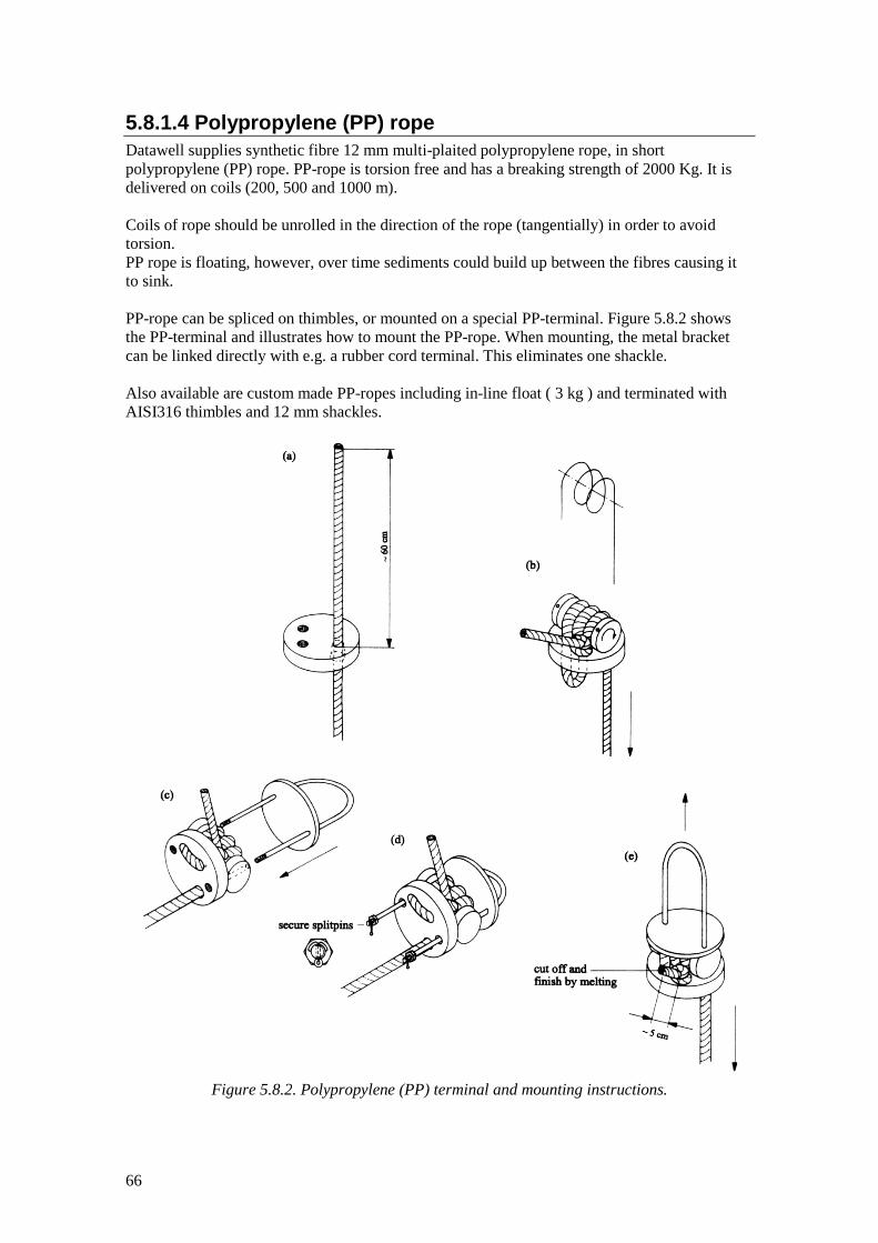
66

5.8.1.4 Polypropylene (PP) rope Datawell supplies synthetic fibre 12 mm multi-plaited polypropylene rope, in short polypropylene (PP) rope. PP-rope is torsion free and has a breaking strength of 2000 Kg. It is delivered on coils (200, 500 and 1000 m). Coils of rope should be unrolled in the direction of the rope (tangentially) in order to avoid torsion. PP rope is floating, however, over time sediments could build up between the fibres causing it to sink. PP-rope can be spliced on thimbles, or mounted on a special PP-terminal. Figure 5.8.2 shows the PP-terminal and illustrates how to mount the PP-rope. When mounting, the metal bracket can be linked directly with e.g. a rubber cord terminal. This eliminates one shackle. Also available are custom made PP-ropes including in-line float ( 3 kg ) and terminated with AISI316 thimbles and 12 mm shackles.

Figure 5.8.2. Polypropylene (PP) terminal and mounting instructions.

67

5.8.1.5 Sinker For larger depths, Datawell provides in-line sinkers which avoid the PP rope coming afloat. The sinker consists of two identical aluminium parts which can be fitted to the 12 mm multi-plaited PP rope supplied by Datawell. Applying or removing the sinkers from the rope can be done without special equipment or small parts. See figure 5.8.3.

Figure 5.8.3. Mounting instruction - aluminium sinker.

68

5.8.1.6 Floats The purpose of floats is to keep the mooring free from the seabed. Datawell provides two types of floats, a 3 Kg and a 10 Kg float. The 0.2 m diameter, 3 Kg buoyancy float can be tied with a 8 mm Nylon rope to the polypropylene rope by two times a clove hitch, see Figure 5.8.4. This way of mounting is called in-line float and it leaves the main rope intact. In this way the strength of the polypropylene rope is not decreased. Its main function is to lift the lower end of the mooring line from the seabed. The working depth of the float is 1.4 Km.

Figure 5.8.4. In-line float (0.2 m diameter, 3 Kg buoyancy) and mounting instruction.

Another float supplied by Datawell has a 0.3 m diameter and provides 10 Kg buoyancy. The float is attached to line terminals in the mooring line with a shackle and split pin or directly linked by a PP terminal (see Figure 5.8.7 ). The larger buoyancy is needed to lift the heavier rubber cord terminals to keep the rubber cord away from the seabed. We advise not to use a float when the seabed is sandy at that location. A sandy seabed does not damage the rubber, making the float more of a hazard than a contribution. The working depth of the 0.3 m diameter float is 1.4 Km too.

5.8.1.7 Rubber cords As mentioned, the rubber cords are essential for high quality wave measurements. They allow the buoy to follow the wave motion, thus guaranteeing that the measured motion of the buoy is indeed the same as the motion of the water due to waves. For a Directional Waverider a rubber cord of 30 m should be used to guarantee good wave following properties even for small motions at low frequencies. Current velocities up to 3 m/s (6 knots) can be accepted. Natural rubber is chosen for its high tear strength and low tear propagation specifications. This reduces chances on mooring failure in operation due to, initially, minor cuts in the rubber cord. The rubber cords are checked for hardness degree, tear strength and tensile strength. The rubber cord is rejected when the strength falls below 50 Kg/cm2 (Delft method). In case of strong breaking waves of the plunging type, the buoy has to be pulled through a wall of water running at considerable velocity. In that case the induced forces may incidentally exceed the breaking strength of the rubber cord. In this situation, the use of a polypropylene safety line parallel to the rubber cord is advised: limiting the maximum elongation of the rubber cord to 4 times the unstretched length, it helps the mooring to survive the peaks of the water forces. Rubber cords are 30 m or 15 m in length, but can be supplied in any length up to 30 m. Available are diameter 27 mm for 0.7 m diameter buoys or 35 mm for 0.9 m diameter buoys.

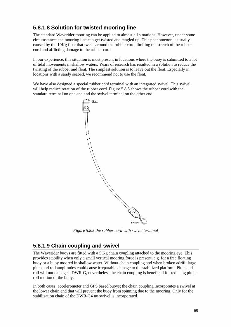
69

5.8.1.8 Solution for twisted mooring line The standard Waverider mooring can be applied to almost all situations. However, under some circumstances the mooring line can get twisted and tangled up. This phenomenon is usually caused by the 10Kg float that twists around the rubber cord, limiting the stretch of the rubber cord and afflicting damage to the rubber cord. In our experience, this situation is most present in locations where the buoy is submitted to a lot of tidal movements in shallow waters. Years of research has resulted in a solution to reduce the twisting of the rubber and float. The simplest solution is to leave out the float. Especially in locations with a sandy seabed, we recommend not to use the float. We have also designed a special rubber cord terminal with an integrated swivel. This swivel will help reduce rotation of the rubber cord. Figure 5.8.5 shows the rubber cord with the standard terminal on one end and the swivel terminal on the other end.

Figure 5.8.5 the rubber cord with swivel terminal

5.8.1.9 Chain coupling and swivel The Waverider buoys are fitted with a 5 Kg chain coupling attached to the mooring eye. This provides stability when only a small vertical mooring force is present, e.g. for a free floating buoy or a buoy moored in shallow water. Without chain coupling and when broken adrift, large pitch and roll amplitudes could cause irreparable damage to the stabilized platform. Pitch and roll will not damage a DWR-G, nevertheless the chain coupling is beneficial for reducing pitch-roll motion of the buoy. In both cases, accelerometer and GPS based buoys; the chain coupling incorporates a swivel at the lower chain end that will prevent the buoy from spinning due to the mooring. Only for the stabilization chain of the DWR-G4 no swivel is incorporated.

70

Two chain thicknesses exist: 20 mm chain with swivel ( DWR-MkIII, WR-SG, DWR-G7 and DWR-G9) and 16 mm chain without swivel (DWR-G4). The chain ends or swivel are connected directly to the mooring eye and the rubber cord terminal by 12 mm shackles with M12 bolt and nut, blocked by a 2x32 mm split pin. Chain coupling, swivel, shackle, bolt, nut and split pin are all made of stainless steel AISI316 and are delivered assembled to the buoy, see Figure 5.8.6.

Figure 5.8.6 Mounting illustrations of a chain coupling for

AISI 316 hull and Cunifer 10 hull.

5.8.1.10 Anodes Corrosion risks of the stainless steel AISI316 buoy hull can be prevented by applying sacrificial aluminium anodes. These anodes are fitted to the chain below the buoy (from the second link from the buoy). In the water an adequate galvanic current path is formed between the anodes and the hull through the chain and back through the sea water. The lay-out of the protective anodes is given in Figure 5.8.7. At least one free link should be left between the clamps and the buoy. To prevent the nuts from unscrewing Nyloc nuts should be used. Nyloc nuts should be used only once. The anodes have an estimated life of three years. Cunifer10 hulls do not require anodes.

71

Figure 5.8.7. Mounting illustration of aluminium sacrificial anodes.

72

5.8.1.11 Standard mooring lay-out Mooring packages are available for each depth range. All components are of high quality to prevent corrosion, and kinking and twisting of the mooring line. Shackles and terminals for easy mounting are included. The main principles underlying the standard mooring ‘recipe’ are:

(1) the configuration must be neutrally buoyant (2) the mooring line length is twice the water depth (3) the polypropylene line length equals two times the water depth (D) minus the rubber

cord length with a minimum of the water depth plus 5 meters for retrieving purposes. (4) there is a clearance at both sea surface and seabed to avoid interference with ships and

wrecks. (5) the ropes are torsion-free to avoid kinking and twisting of the rope and spinning of the

buoy. The rubber cord has a length of 30 m for the Directional Waveriders and 15 m for non-directional Waveriders. The length of the polypropylene line depends on the low tide depth of the water, henceforth indicated by D. A sketch of the mooring is found in Figures 5.8.8(a)-(e). Datawell rubber cords come in two diameters. To provide the same flexibility to ride the waves, 0.9 m diameter buoys must be fitted with 35 mm rubber cords and the smaller 0.7 m diameter buoys must be fitted with the thinner 27 mm rubber cords. Due to its small size and little residual buoyancy the 0.4 m DWR-G is to be used as a free-floating buoy. However a mooring is available for currents up to 2 kn, please refer to chapter 5.8.2. Sediments can build up in the open structure of the polypropylene rope. In time the rope can become sinking instead of floating. To avoid entanglement of the rope a small in-line float (buoyancy 3 Kg) in the PP-rope, a few metres above the seabed, is advised.

Table 5.8.1 Number of sinkers and floats for various water depths (D)

DIRECTIONAL WAVERIDER

8 m < D < 17 m 2 floats 1 sinker 17 m < D < 35 m 1 float 1 sinker 35 m < D < 60 m 60 m < D < 85 m 1 sinker 85 m < D < 150 m 2 sinkers 150 m < D < 200 m 3 sinkers

WAVERIDER 8 m < D < 17 m 1 float 1 sinker 17 m < D < 30 m 30 m < D < 75 m 1 sinker 75 m < D < 140 m 2 sinkers 140 m < D < 200 m 3 sinkers

73

Figure 5.8.8(a) Mooring line layout for the (Directional) Waverider.

74

Figure 5.8.8(b) Mooring line layout for the (Directional) Waverider.

75

Figure 5.8.8(c) Mooring line layout for the (Directional) Waverider.

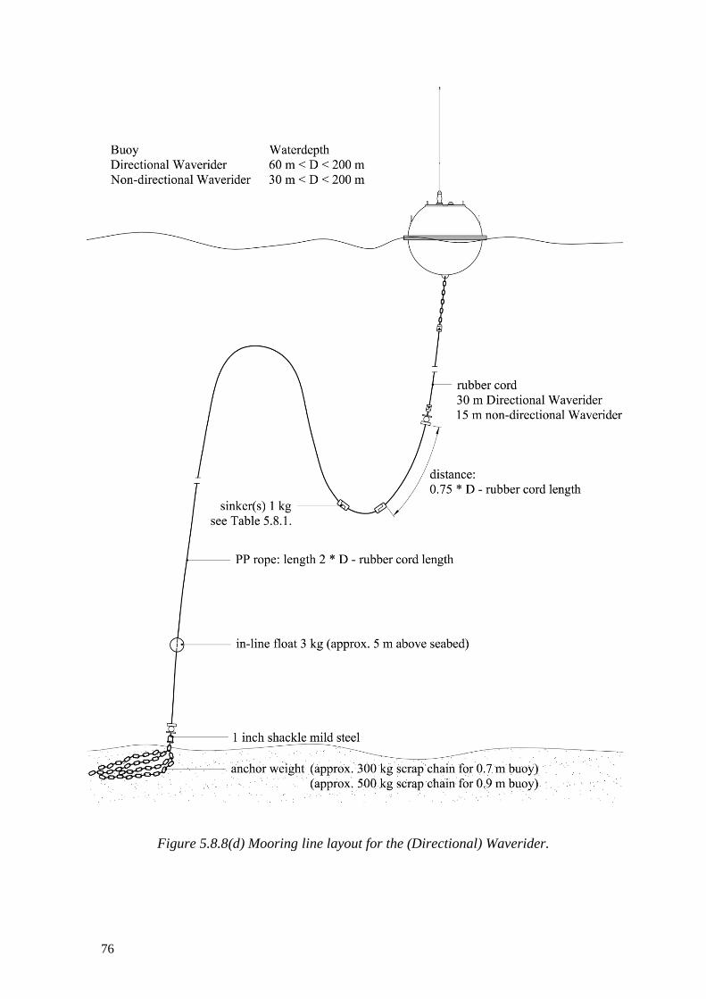
76

Figure 5.8.8(d) Mooring line layout for the (Directional) Waverider.

77

Figure 5.8.8(e) Mooring line layout for the (Directional) Waverider.

78

5.8.1.12 Applicability of the standard mooring lay-out In Table 5.8.2 below, it is indicated up to what depth the standard mooring applies. If the local current strength corresponds to the entry in the first column, then the depth in the second column in the same row is the maximum depth up to which the standard mooring applies. The current is assumed to extend over the full depth.

Table 5.8.2. Applicability of the standard mooring lay-out. Current speed (m/s) Max. depth

0.7 m buoy Max. depth 0.9 m buoy

0.5 1050 2000 1.0 180 330 1.5 61 120 2.0 28 62 2.5 19 42 3.0 15 34

Contact Datawell for a fine-tuned mooring advice, if your location is not covered by the table. Examples: • If e.g. at the intended location the current speed is 1.5 m/s (3 knots) and the depth is 100 m,

then the standard mooring applies for a 0.9 m buoy. • Should the depth be 150 m, then the mooring must be reconsidered. If the current is indeed

over the full depth, the remedy is a subsurface float (contact Datawell Sales for a customized mooring design).

• Idem 150 m depth, in case the current is only over the upper half of the depth, the standard mooring still applies.

5.8.1.13 Mooring preparation On your request a tailor-made mooring with appropriate lengths and all terminals attached will be shipped to you. You only have to provide for an anchor weight. Connect all cords, ropes and wires according to the standard mooring lay-out or to the customized lay-out included in the shipment. To avoid entangling the mooring line, we advise to lay it out on the deck of the ship with alternate left and right turns. In case of a long mooring line stow the mooring line as a stack of ‘eights’ (8) with the buoy end up and the anchor end down. To keep everything in place you may tie a rope through each loop and around the waist. When pulling rope or wire of the reel do not slide of loops but unroll it. Not only will the line become hard to handle, it will also build up torsion that may set the buoy spinning and damage the motion sensor. In practice, all these actions will be taken when the ship has already left the port. However, to avoid problems at sea please inspect the mooring once before you actually deploy the buoy. If this is your first buoy deployment, lay out the mooring on land at ease as an exercise. study it and pack it into the blue containers again.

79

5.8.1.14 Deployment Once you have set up and checked the equipment on land, itis time to deploy the buoy. A safe and successful deployment requires the right equipment and a well-thought out procedure. Please read the Dangers and warnings and the Mooring preparation sections again for your own safety and comfort. Bring a few ropes and a knife, they always come in handy. Also bring a used car-tire to support the buoy while on deck. Still the buoy must be roped to the railing. You may bring the (portable) receiver and a receiving antenna to monitor the buoys outputs. Alternatively you can radio contact your receiving station during deployment. The best time to do this is after the buoy is deployed on its location and before the ship will return to port. To handle the weight of the anchor weight, either a ship with a hoisting crane or U-frame or a ship with a removable railing should be chartered. For comfortable deployment a day with small waves is best waited for. The procedure in Figure 5.8.9 is suggested for a small vessel with a hoisting crane or removable railing in the front. Users should adapt the procedure to size and outfit of their ship and according to their own experience. Before the actual deployment lay out the mooring line on deck and connect the ends to the anchor weight and buoy using the shackles and split pins(a). If you use the 8-shaped pack with tiers, remove the tiers just before launching. Never stand inside the loops of the mooring line or between the mooring line and the ship sides. Hoist the anchor weight on the side of the ship and hang it overboard on a rope (b) or push it towards the removable railing but not over. Release the anchor weight from the hoisting crane and leave it hanging overboard. Once you are at the intended location steer the ship in reverse backing up against the current (c). This manoeuvre will keep the mooring line out of the screw propeller. Deploy the buoy by hoisting (d) or pushing it overboard. If you hoist the buoy, use an extra piece of rope to keep the crane hook at a distance from the antennas. To release, cut the rope. The buoy may be safely dropped from a height of 2 m. Give the line sufficient slack before dropping the buoy, so it will not be pulled upside down. Keep the line slack, running out the line loop by loop while the buoy drifts away from the ship (e). Finally, cut the rope that carries the anchor weight or push the anchor weight overboard (f). Do not use your hands, you may get entangled. Continue to back up until the ship has gained enough distance to steer clear of the buoy and mooring line.

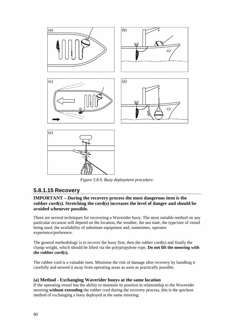
80

Figure 5.8.9. Buoy deployment procedure.

5.8.1.15 Recovery IMPORTANT – During the recovery process the most dangerous item is the rubber cord(s). Stretching the cord(s) increases the level of danger and should be avoided whenever possible. There are several techniques for recovering a Waverider buoy. The most suitable method on any particular occasion will depend on the location, the weather, the sea state, the type/size of vessel being used, the availability of substitute equipment and, sometimes, operator experience/preference. The general methodology is to recover the buoy first, then the rubber cord(s) and finally the clump weight, which should be lifted via the polypropylene rope. Do not lift the mooring with the rubber cord(s). The rubber cord is a valuable item. Minimise the risk of damage after recovery by handling it carefully and stowed it away from operating areas as soon as practically possible. (a) Method - Exchanging Waverider buoys at the same location If the operating vessel has the ability to maintain its position in relationship to the Waverider mooring without extending the rubber cord during the recovery process, this is the quickest method of exchanging a buoy deployed at the same mooring:

81

Lift the buoy from the water using a rope bridal, connected between the two handles fitted to the upper half of the Waverider buoy hull. Steady or anti-spin lines can be attached to the safety triangle during the lifting procedure. Stow and secure the buoy on the vessel deck. Secure the mooring to the deck at the upper end of the Polypropylene rope. Disconnect the mooring between the chain coupling of the buoy and the rubber cord terminal. Connect the mooring to the chain coupling of the replacement buoy, ensuring that the safety shackle is correctly fitted and securely locked with nut and split pin. Free all securing lines to the mooring and the Waverider buoy, lift the buoy and lower back onto the water. During the above operation a member of the recovery team, equipped with a knife, should be stationed close to the secured rubber cord. Should any sudden vessel movement increases the tension in the rubber cord and endanger the recovery personnel, the rubber cord must be severed. It should be noted that this mode of operation may only be used where the ship is able to maintain its exact position within a couple of meters. Additionally this method does not allow all the mooring to be fully inspected (the rubber cord(s) for cuts and polypropylene rope for wear). If this method is regularly used, increased inspections of the complete mooring must be undertaken. (b) Method - Recovery using a dummy buoy Where there is no replacement Waverider buoy, a dummy buoy can be deployed to support the mooring thus avoiding the need to retrieve the complete mooring. An old Waverider equipped with an operating flashlight may be used as a dummy buoy. In this instance the exchange procedure described in a) above has to be applied twice. (c) Method - Recovery using a small work boat, rib or dingy The Waverider cannot be lifted onto a small workboat or rib. However, such a vessel may be used to tow the Waverider buoy to a larger vessel or ashore. Mooring recovery will be by hand, ensuring that no tension is placed on the rubber cord(s). Recovery of the mooring clump weight must only be achieved by using the polypropylene rope. If the mooring clump weight cannot be recovered, the polypropylene rope may be cut below the rubber cord leaving the clump weight and residue rope on the seabed. The Waverider should not be towed at speeds greater than 2 m/s (4 kn). By using this recovery method, the cost of the loss of a section of mooring line and clump weight would be more than offset by the savings made in not chartering a ship.

5.8.1.16 Mooring hazards The phenomenon most likely to result in early failure of the mooring is galvanic corrosion between different metals in sea water. When a mild steel shackle is coupled to the AISI316 stainless steel Waverider the shackle may fall apart within one month. Even the coupling of AISI304 and AISI316 stainless steel will lead to early failure. In case it is necessary to couple different metals, an electrically insulating element should be used. Kinking may also result in failure of the mooring. Synthetic fibre ropes are apt to kink when the rope has an asymmetrical (layed) construction, but the braided and plaited constructions are free from torsion when loaded and therefore not liable to kinking. At the end of the chain coupling a swivel is placed for extra safety. The swivel is made from AISI316 material with a thrust bearing and a self-lubricating Nylon ring placed in between the steel faces.

82

Another cause of failure was found to be that the screwed parts of a mooring unscrewed themselves. Therefore, the number of screwed parts should be reduced to a minimum. Nuts must be secured with a steel ring or split pin placed in a hole through the threaded part above the nut. The screwed pins of shackles should be properly housed with metal wire of the same composition as that of the shackle or with Nylon cord or patented Nylon tiers. Make sure that Nylon tiers do not contain metal parts. Three further causes of mooring failure are due to human interference. The first one is the cutting of the mooring line by ships passing the buoy too closely. The second one is human curiosity and stealing. Informing the local public of the importance of wave information and of the role of the Waverider may reduce their interference. Furthermore, the salvage reward should not be too tempting. The third one is the use of the Waverider as a mooring buoy for small boats.

Mooring 40cm buoys 5.8.2When free floating, the 40 cm diameter DWR-G4 measures as accurately as its larger brothers, the DWR-G7 and DWR-G9. Obviously, the mooring of such a small buoy is a challenge. The resistance of the buoy to getting submerged by the mooring forces is very small. Furthermore, care should be taken that the mooring is sufficiently flexible to allow the buoy to follow the vertical and horizontal wave motion adequately.

5.8.2.1 Mooring inspection Verify with Datawell whether your mooring is suitable for your local conditions before you deploy the buoy at the preferred location. Inspection of the Dyneema line may show signs of wear.

5.8.2.2 Mooring parts The correct mooring of a wave buoy is essential to measuring wave parameters according to specifications. The design of an appropriate mooring requires knowledge of the current speed and profile, the depth, tides and wave height. To help our customers in finding a good mooring solution, Datawell has developed a standard mooring lay-out for your DWR-G 0.4 m wave buoy. First, a general remark on mooring materials is made. After that, all parts of the mooring are described in more detail. Finally, attention is given to complete mooring lay out and the effect of depths and currents. Note that the DWR-G 0.4 m buoy is also used free-floating with only a stabilization chain. In a marine environment corrosion is a problem and stainless steel parts are crucial for the longevity of the mooring and buoy. All metal parts supplied by Datawell, such as the chain and metal parts of the terminals, are of AISI316 stainless steel. Every production run is sampled for all separate elements and tested to ensure that the composition lies within AISI316 specifications. Nevertheless, it is advisable to use protective anodes whenever the buoy is used for longer periods in a row. Datawell can supply the stabilization chain including anodes, see figure 5.8.10.

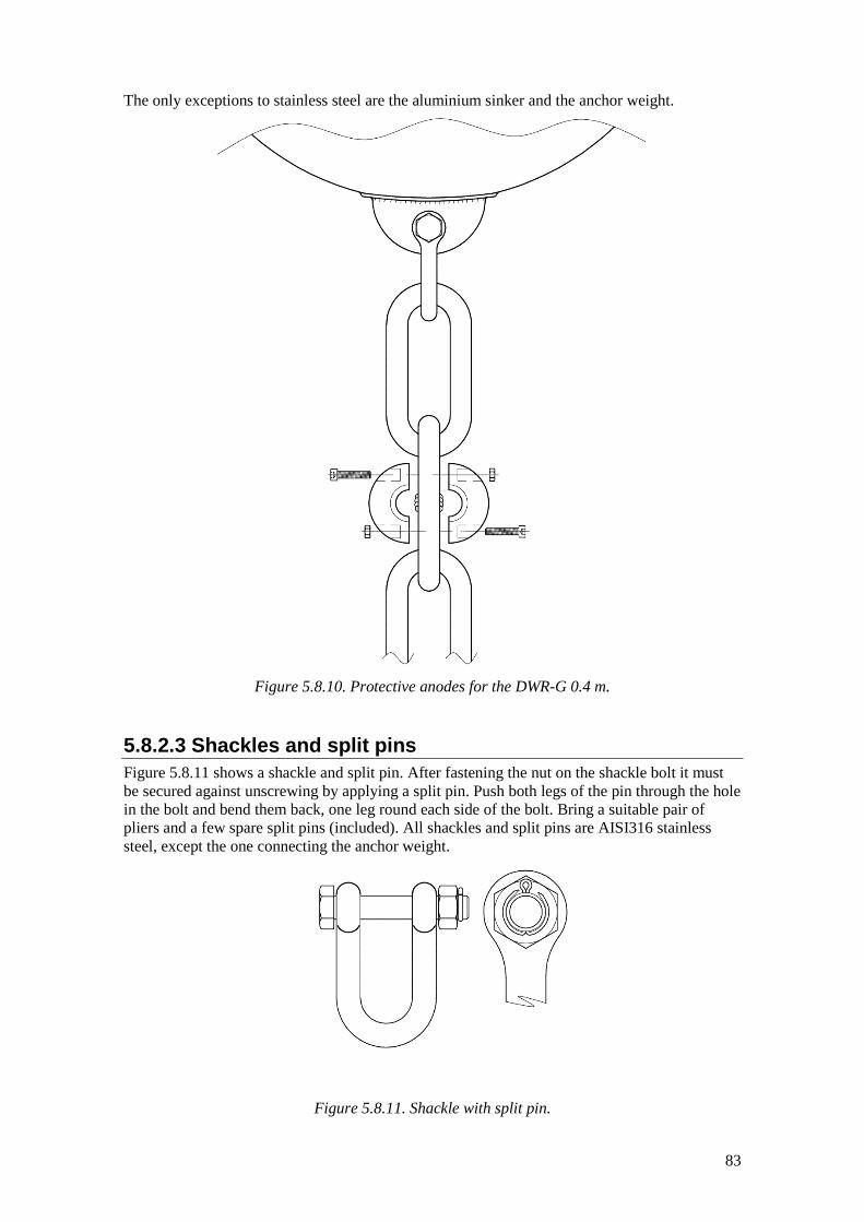
83

The only exceptions to stainless steel are the aluminium sinker and the anchor weight.

Figure 5.8.10. Protective anodes for the DWR-G 0.4 m.

5.8.2.3 Shackles and split pins Figure 5.8.11 shows a shackle and split pin. After fastening the nut on the shackle bolt it must be secured against unscrewing by applying a split pin. Push both legs of the pin through the hole in the bolt and bend them back, one leg round each side of the bolt. Bring a suitable pair of pliers and a few spare split pins (included). All shackles and split pins are AISI316 stainless steel, except the one connecting the anchor weight.

Figure 5.8.11. Shackle with split pin.

84

5.8.2.4 Dyneema rope Datawell supplies 6 mm Dyneema rope, Dyneema rope is torsion free and has a breaking strength of 2000 Kg. Dyneema rope is floating, however, over time sediments could build up between the fibres causing it to sink. Dyneema rope can be mounted on a special Dyneema terminal. The Dyneema terminal allows you to adjust the length of the rope for future mooring lengths. Figure 5.8.12 shows the Dyneema terminal and illustrates how to mount the Dyneema rope. When mounting the stainless steel bracket can be linked directly with the shackle attached to the mooring weight. No split pins are used in this design to secure the nuts. After fastening the nuts, force them in to the black Delrin material (a), when pulling at the stainless steel bracket (b).

Figure 5.8.12. Dyneema terminal and mounting instructions.

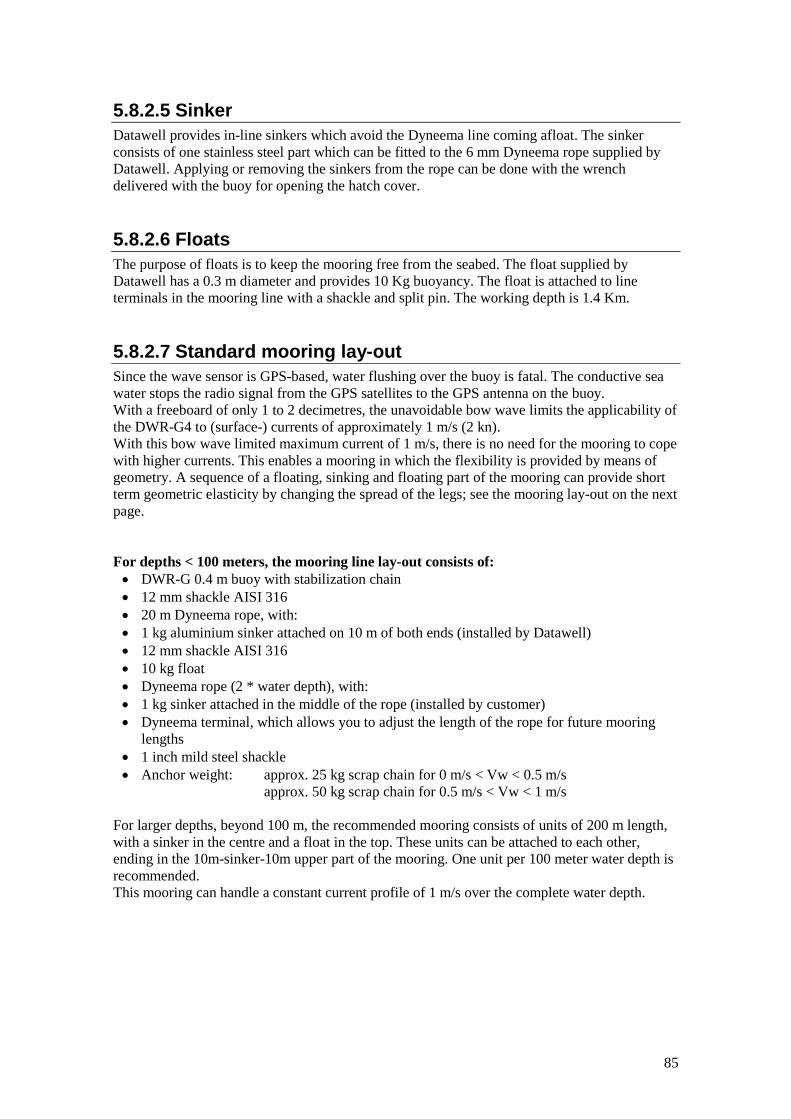
85

5.8.2.5 Sinker Datawell provides in-line sinkers which avoid the Dyneema line coming afloat. The sinker consists of one stainless steel part which can be fitted to the 6 mm Dyneema rope supplied by Datawell. Applying or removing the sinkers from the rope can be done with the wrench delivered with the buoy for opening the hatch cover.

5.8.2.6 Floats The purpose of floats is to keep the mooring free from the seabed. The float supplied by Datawell has a 0.3 m diameter and provides 10 Kg buoyancy. The float is attached to line terminals in the mooring line with a shackle and split pin. The working depth is 1.4 Km.

5.8.2.7 Standard mooring lay-out Since the wave sensor is GPS-based, water flushing over the buoy is fatal. The conductive sea water stops the radio signal from the GPS satellites to the GPS antenna on the buoy. With a freeboard of only 1 to 2 decimetres, the unavoidable bow wave limits the applicability of the DWR-G4 to (surface-) currents of approximately 1 m/s (2 kn). With this bow wave limited maximum current of 1 m/s, there is no need for the mooring to cope with higher currents. This enables a mooring in which the flexibility is provided by means of geometry. A sequence of a floating, sinking and floating part of the mooring can provide short term geometric elasticity by changing the spread of the legs; see the mooring lay-out on the next page. For depths < 100 meters, the mooring line lay-out consists of: • DWR-G 0.4 m buoy with stabilization chain • 12 mm shackle AISI 316 • 20 m Dyneema rope, with: • 1 kg aluminium sinker attached on 10 m of both ends (installed by Datawell) • 12 mm shackle AISI 316 • 10 kg float • Dyneema rope (2 * water depth), with: • 1 kg sinker attached in the middle of the rope (installed by customer) • Dyneema terminal, which allows you to adjust the length of the rope for future mooring

lengths • 1 inch mild steel shackle • Anchor weight: approx. 25 kg scrap chain for 0 m/s < Vw < 0.5 m/s

approx. 50 kg scrap chain for 0.5 m/s < Vw < 1 m/s For larger depths, beyond 100 m, the recommended mooring consists of units of 200 m length, with a sinker in the centre and a float in the top. These units can be attached to each other, ending in the 10m-sinker-10m upper part of the mooring. One unit per 100 meter water depth is recommended. This mooring can handle a constant current profile of 1 m/s over the complete water depth.

86

For depths > 100 meters, the mooring line lay-out consists of: • DWR-G4 buoy with stabilization chain • 12 mm shackle AISI 316 • 20 m Dyneema rope, with: • 1 kg aluminium sinker attached on 10 m of both ends (installed by Datawell) • 12 mm shackle AISI 316 • For every 100 meters water depth, N times the following mooring is needed:

For example: Depth is 225 meters N = 2 Depth is 370 meters N = 3

• 10 kg float • 200 m Dyneema rope, with: • 1 kg sinker attached in the middle of the rope (installed by Datawell) • 12 mm shackle AISI 316 • Anchor weight: approx. 25 kg scrap chain for 0 m/s < Vw < 0.5 m/s

approx. 50 kg scrap chain for 0.5 m/s < Vw < 1 m/s

87

Figure 5.8.13. (a) Mooring line lay-out for the DWR-G 0.4 m.

88

Figure 5.8.14. Mooring line lay-out for the DWR-G 0.4 m.

89

5.8.2.8 Mooring preparation On your request a tailor-made mooring with appropriate lengths and all terminals attached will be shipped to you. You only have to provide for an anchor weight. Connect all ropes according to the mooring lay-out. To avoid entangling the mooring line, lay it out on the deck of the ship with alternate left and right turns. In case of a long mooring line stow the mooring line as a stack of ‘eights’ (8) with the buoy end up and the anchor end down. To keep everything in place you may tie a rope through each loop and around the waist. In practice, all these actions will be taken when the ship has already left the port. However, to avoid problems at sea please inspect the mooring once before you leave the port and actually deploy the buoy. If this is your first buoy deployment, lay out the mooring on land at ease as an exercise, study it and pack it up again.

5.8.2.9 Deployment Once you have set up and checked the equipment on land, itis time to deploy the buoy. A safe and successful deployment requires the right equipment and a well-thought out procedure. You may bring the (portable) receiver and a receiving antenna to monitor the buoys outputs in case your buoy is equipped with the HF communication link. Alternatively you can radio contact your receiving station during deployment. The best time to do this is after the buoy is deployed on its location and before the ship will return to port. Before the actual deployment lay out the mooring line on deck and connect the ends to the anchor weight and buoy using the shackles and split pins. Never stand inside the loops of the mooring line or between the mooring line and the ship sides. Once you are at the intended location steer the ship in reverse backing up against the current. This manoeuvre will keep the mooring line out of the screw propeller. Deploy the buoy by gently pushing it overboard. The buoy may be safely dropped from a height of approximately 3 m. Give the line sufficient slack before dropping the buoy, so that it will not be pulled upside down. Keep the lines slack, running out the line loop by loop while the buoy drifts away from the ship. Finally, push the anchor weight overboard. Continue to back up until the ship has gained enough distance to steer clear of the buoy and mooring line. Though deploying the buoy by attaching a rope to the buoy handles is still the most recommended procedure, a correctly mounted triangle can also be used to hoist the buoy.

90

5.9 Hull and hatchcover Hull and hatchcover form a watertight compartment that provides buoyancy and houses batteries, sensors and electronics. This section only describes all items on the exterior and some basic functions in the interior of the compartment. Separate sections are devoted to battery compartments, electronics unit, motion sensors and temperature sensor.

Packing frame and buoy weights 5.9.1For safe transportation the buoy must be packed in the packing frame in which it arrived originally. It is advisable to leave the buoy in its packing frame during all transport. To take the buoy out of the frame, just remove one of the poles and slide the buoy out of the frame. Use a hoisting crane to support the buoy. For handling and transport see Table 5.9.1 with dimensions and weights.

Table 5.9.1. Buoy and packing frame weights and dimensions. Buoy 0.4 m 0.7 m 0.9 m

DWR-G DWR-MkIII DWR-G/ WR-SG

WR-SG DWR-MkIII/ DWR-G

Approximate buoy weight including batteries, antennas and chain (AISI316 and Cunifer10 (Cu) )

17 Kg

105 Kg 111 Kg (Cu)

95 Kg 101 Kg (Cu)

150 Kg 161 Kg (Cu)

225 Kg 236 Kg (Cu)

Packing frame weight 6.5 Kg 35 Kg 45 Kg Frame height 0.77 m 1.20 m 1.42 m Frame width/buoy width (including fender)

0.46 m 0.78 m 1.0 m

Buoy height (as transported, mooring eye-hatchcover handles)

0.50 m 0.73 m 0.95 m

For testing purposes it may be helpful to put or leave the buoy in the frame, e.g. pitch, roll and horizontal accelerometers tests. This setup is not suitable for testing the fluxgate compass as the metal parts of the packing frame can influence the compass reading.

Hull, Cunifer10, corrosion and painting 5.9.2The hull has three functions: providing buoyancy and protecting the sensors and electronics inside from water and impacts. While doing so it faces three enemies: ship collisions, corrosion and fouling. At 0.9 m diameter the buoyancy force initially increases 62 N with every cm of immersion. Just before full immersion the buoyancy of a 0.9 m diameter hull including chain is 1630 N. For loads on the buoy larger than this threshold the buoy will sink. Datawell hulls are designed to withstand head-on collisions. Ship collisions typically are not fatal although the buoy will be dented. If the propeller screw hits the buoy, then the buoy will be damaged but even than it can often be repaired. The hull of the Waverider stays watertight even if largely deformed. Cunifer10 (copper-nickel alloy) is also available as hull material, see below. Though its strength is less than that of stainless steel, it can take large deformations. It is known that the corrosion risk of unprotected AISI316 stainless steel is to a certain degree unpredictable. Pitting is the predominant form of observed corrosion. However, sacrificial

91

anodes on the stabilizing chain below the hull will mainly take care of corrosion of the AISI316 stainless steel hull. The use of sacrificial anodes is strongly recommended, even for painted buoys. Without protecting anodes, blistering paint or pinholes in the paint cause accelerated local pitting of the AISI316 stainless steel. Pitting has been found to be aggravated by the use of paints containing chlorinated hydrocarbons, acids or reducing agents. Depending on local conditions such as water temperature and water quality, anti-fouling paint may be necessary. Severe fouling may affect the mooring performance due to increased drag. As alternative to anti-fouling paint we supply buoys with a Cunifer10 hull. Cunifer 10 is a copper-nickel alloy which does not pit and reduces fouling. Paint may be applied on a AISI316 hull for protection against pitting, better visibility or because of navigation regulations. For painting we recommend the Brantho Korrux “3 in 1” (RAL 1021) paint system which has proven its quality in a maritime environment. After removing the fender, degreasing the hull (preferably by sanding), making it dust free and covering flange, handles and mooring eye, Brantho Korrux can easily be applied in 3 layers without sanding the previous layer. Each layer needs to dry for 48 hours before the next layer can be applied. After the third finishing layer the paint must be allowed to dry for at least 2 weeks before mounting the fender. Brantho Korrux is available in cans of 750 ml (painting materials and instructions are included). For galvanic and anti-fouling reasons we strongly advise to paint only the upper half of a Cunifer10 hull.

Mooring eye 5.9.3The mooring eye is located underneath the hull and is used to attach the mooring. It is made of the same material as the hull.

Fender 5.9.4The fender serves no wave measuring purpose, although it may damp resonant pitching, rolling and immersing somewhat. It mainly protects users from the sharp welding edge of the two hull semi-spheres when handling the buoy on deck or in a laboratory. It measures 0.46 m, 0.78 m or 1.00 m for the various hull diameters. To inspect for corrosion under the fender you may force it off and on.

Anti-spin triangle 5.9.5To protect the motion sensor in the DWR-MkIII and WR-SG, the installation of an anti-spin triangle is highly recommended in the following situations: in case the buoy is washed ashore, if nearby passing ships are to be expected or if the buoy is transported out of its packing frame. The DWR-G motion sensor is not susceptible to spinning and therefore an anti-spin triangle is not required. Figure 5.9.1 shows how to place the triangle on the fender and fasten the bolts. Sacrificial anodes that fit around the tubes are available to protect the stainless steel triangle from corrosion. The anti-spin triangle can also be used to hoist the buoy in a retrieving/deployment procedure, provided that the triangle is mounted correctly.

92

Figure 5.9.1. Anti-spin triangle mounting on a Waverider buoy.

Handles 5.9.6When lifting or moving the buoy you can use the two handles welded onto the hull. Two handles must be used to carry the load of the whole buoy. The handles on top of the hatchcover are meant to handle the hatchcover only, not the whole buoy. The DWR-G4 buoy is fitted with a hauling rope between the two handles as a standard.

Flange, serial number and FS direction 5.9.7The interior of the buoy can be accessed through the flange. Almost all parts within the hull can be serviced or even replaced through this flange. A small face on the side of the flange indicates the Forward Ship (FS) direction. Horizontal accelerometers, compass and pitch-roll sensors of the DWR-MkIII are referenced to this direction, see subsection 5.4.2. The number engraved on the face itself indicates the hull serial number.

Drying agent bags, plywood 5.9.8As mentioned only a few items on the interior will be described here. To protect the electronics inside the hull from condensing water vapour two bags of drying agent are packed in the hull. Perforated sealing bags are used to slow down the drying process. The colour of the humidity indicator should be blue. If the colour has turned pink, the paper bags (without plastic sealing bag) should be dried at a maximum temperature of 110 ºC for 12 hours. After drying, put the paper bag back into the plastic bag. To prevent unnecessary moisture saturation of the drying

93

agent, close the hatch whenever the buoy is not in use. The bags are fixed to the plywood boards with Velcro straps. Four plywood boards hold down the batteries in the outer ring and the aluminium lid on the aluminium can. In the DWR-G 2 boards are used.

Intelligent Test box, step-up converter and 5.9.9connector pin assignment

An (intelligent) test box is mounted inside the hull or integrated in the main hatchcover cable to monitor battery sections and, in case of the 0.9 m DWR-MkIII, analog sensor outputs, see Figures 5.10.1-5.10.7. Each battery section may be tested by applying a voltmeter over the point “+Bat” and the respective section point “A”, “B”, “C”, etc. These points are interconnected through diodes to point “−Bat”. The standard power supply module only accepts battery voltages in a certain range. A series of 4 cells, as in the DWR-G 0.4 m, produces a series voltage that already lies below this range when the batteries are fresh, let alone when they are nearly exhausted. Therefore, a step-up converter is integrated in the test box. The battery voltage before stepping-up is measured at the points on either side of the connector. Table 5.9.3 displays the scaling of the various analog signals. Note that the sine of the pitch and roll angles is actually measured and not the angle itself. The output resistance of the analog outputs is 4.7 KΩ. Finally the abovementioned figures also show the pin assignment of the main hatchcover connector.

Table 5.9.3. Scaling factors of the analog signal on the test box.

Signal Scaling Av 4000 mV/10.0 m/s2 Ax, Ay 4000 mV/9.82 m/s2 Hx, Hy, Hz 70 mV/A/m Pitch, roll 4000 mV/sin(90º)

Hatchcover and option ports 5.9.10The hatchcover includes 2 or 3 option ports to accommodate several different antennas. It is fastened with 24 hexagon socket screw-bolts in countersinking holes. In case of partial vacuum in the hull, the hatchcover may be lifted by screwing one of the hexagon socket screws in the additional threaded lifting hole. When closing the hatchcover, carefully inspect the rubber sealing ring and the groove in the flange for dirt, cuts and scratches. Take care that the rubber sealing ring is properly fitted in the groove before positioning the hatchcover. Do not over-tighten the screws-bolts, especially Cunifer10 is vulnerable for abuse. Figure 5.9.2 shows the top and bottom side of the hatchcover. The hatchcover of the 0.4 m buoy does not have option ports. It has 8 screw holes. All antennas are permanent. On the bottom side of the hatchcover the electronics unit is fixed with three removable feet. The top side either has two or three option ports labelled HF and GPS. The possible third port depends on the GSM or satellite link used. Each port receives the respective communication antenna and the construction is similar to that of the hatchcover and the hull flange. When placing the respective insert an electrical coaxial connection is made simultaneously. Unused ports should be closed with a blind flange. All ports and connectors are waterproof. Hence, even

94

with unclosed ports or damaged and leaking inserts no water can enter the hull. Nevertheless, short-circuiting the connector may affect the buoy operation. The hatchcover handles are solely intended for lifting the hatchcover with electronics unit and antennas. They must not be used for lifting the complete buoy.

Figure 5.9.2. (a) Top and (b) bottom side of the hatchcover.

95

Radar reflectors 5.9.11Radar reflectors are available for the DWR MkIII and Waverider SG buoys with a 475 mm hatchcover. Two radar reflectors can be fitted on the hatchcover in order to gain an omnidirectional radar reflecting system. This radar reflecting system doubles the buoys visibility on a 3 GHz radar while on a 10 GHz radar the buoy will be ten times better visible. The radar reflectors are made from corrosion resistant stainless steel. Please follow the mounting instructions as delivered together with the radar reflectors and note that we recommend 1 week for the lute which glues the radar reflectors to the hatchcover surface to cure before the buoy can be deployed.

5.10 Power supply and consumption The standard power supply for Datawell buoys are non-rechargeable (= primary) batteries to guarantee autonomous operation under all conditions. Optional a solar system can be installed consisting of a solar panel and Boostcap capacitors for temporarily solar energy storage. Datawell supplies two types of primary alkaline cells, magnetic and non-magnetic cells. The DWR-MkIII buoy specifically requires non-magnetic batteries in order not to disturb the magnetic compass. Operational life of the buoy on a standard set of batteries depends on the number and energy content of the batteries, on the set of buoy functions and options and, most important, if the batteries are used in a continuous period. If the batteries are used with large intervals, the battery life will rapidly deteriorate.

Table 5.10.1 Operational life in months based on Datacell batteries

DWR-9 DWR-7 DWR-G9 DWR-G7 DWR-G4 WR-SG9 WR-SG7

HF 49 16 28 14 1 37 18 A 79 26 34 16 1 77 38 A/HF 40 13 27 13 1 30 15 GSM 79 26 34 16 1 77 38 GSM/HF 40 13 27 13 1 30 15 SBD 83 27 34 16 N/A 84 42 SBD/HF 40 13 27 13 N/A 31 15 Iridium 77 i 24 i 33 i 16 i N/A 69 i 34 i Iridium/HF 38 i 13 i 26 i 13 i N/A 29 i 14 i

i Based on a transmission interval of 30 minutes.

Datacell primary and secondary cells 5.10.1At the moment Datawell supplies 3 cell models as listed in Table 5.10.2. The voltage per cell is about 1.6 V for fresh cells and 0.7 V for exhausted cells. Self-discharge of the cells is less than 2% per year. All cells have a cylindrical shape with a diameter of 65 mm and a height of 205 mm (including connectors). Different connectors are used for the anode in the centre and the cathode near the edge to prevent reversed cells in a series connection. Batteries have a best before date imprinted on it which also serves as a batch number.

96

Table 5.10.2. Overview of batteries for Datawell buoys. Manufacturer Cell

colour Type Technology Energy content

(Wh) Magnetic* Primary or

Secondary Datacell Green RC27G alkaline 270 yes Primary Datacell Black RC27B alkaline 270 No Primary

*magnetic cells should not be used in DWR-MkIII buoys

Battery status 5.10.2With help of Table 5.10.3 the battery status bits may be translated into weeks left before the buoy runs out of energy. There are two methods to determine the remaining operational life. One is to measure the voltage and to relate this to the battery discharge curve. However, on a nearly horizontal part of the discharge curve this is not very accurate. The second method in fact integrates the discharge curve yielding energy delivery or consumption versus time. This method is applied in the power consumption meter of the DWR-MkIII, DWR-G and WR-SG buoys. In case the buoy is equipped with the solar system this operating lifetime can be regarded as absolute minimum. Note that the operational life tol is also given directly in word 6 of the system file, see Table 5.7.4.

Table 5.10.3. Translation of battery status in the system file to remaining operational time. Lifetime prediction is based on primary cell use only. In case the buoy is equipped with the

solar system this life time can be regarded as absolute minimum. Battery status

Remaining operational life (weeks)

0 0 – 6 1 7 – 15 2 16 – 22 3 23 – 27 4 28 – 41 5 42 – 49 6 50 – 60 7 61 - or more

Hybrid power option 5.10.3On all buoys, except the DWR-G4 and WR-SG, a solar system can be installed. Together with the primary cells this makes the hybrid power system. The purpose of the hybrid power option is to reduce primary battery drainage. The solar system of the DWR-MkIII consists of a solar panel on the hatchcover and a set of Boostcap capacitors in the hull for temporarily solar energy storage. The solar system of the DWR-G consists only of a solar panel because of the higher power consumption of this buoy. This concept combines the reliability of primary cells with the availability of solar energy. The life time expectancies as presented in this manual and in the messages of the buoy are always without solar energy contribution, and thus can be regarded as minimum life expectancies. When installed, the lifetime expectancy of a hybrid buoy presented in the W@ves21 software can fluctuate. This depends on the total amount of sunlight.

97

5.10.3.1 Solar panel The solar panel array converts the captured sunlight into electrical energy. Due to the low power consumption of the Waverider only a small solar panel is required. The array comprises a flat circle of 5 x 5 cm2 solar cells on top of the stainless steel hatch-cover and is protected by a layer of polycarbonate. This rugged construction, fully integrated within the original spherical design of the hull, makes the panel robust. Using only 16 of these small cells, the array generates a peak power of 15 times the continuous power consumption of a Directional Waverider (specified at air mass 0).

Figure 5.10.1. Solar panel array with cells linked in series (A, left) or in matrix (B, right).

During even reasonably short deployments, surface floating buoys such as the Waverider cannot avoid suffering from marine growth, salt crystals, bird deposits and physical knocks. Shadows cast by the antennae and fixings will also intrude between the sun and the solar cells. Therefore, a novel cell configuration has been used to deal with these situations. Usually a solar panel array consists of many small solar cells connected in series. When a shadow blocks light to an individual cell or a cell is damaged, the chain is broken and the whole section stops producing energy (see Fig 5.10.1A). The solar panel array on the Waverider overcomes this potential problem by linking the solar cells in a matrix (see Fig 5.10.1B). When any one cell is blocked, current can still flow through the neighbouring cells in the matrix. In the unlikely case that a complete row in the matrix is blocked, no more current would flow but the probability of this happening is minimised by placing the individual cells of a row as remote as possible from each other.

5.10.3.2 Boostcap capacitors The most innovative feature of the hybrid Waverider is the Boostcap capacitor. An array of these specialised, ultra-high capacity capacitors is used to store surplus solar energy during the day. A normal power supply capacitor typically has a capacity of 0.0047F (Farad = unit in which capacity is expressed). Boostcaps are available in capacities up to 2600F (2.5 Volt). That is half a million times more than a normal power supply capacitor. Although Boostcaps do not come anywhere near the storage capacity of lead-acid batteries, the extremely efficient, low power consumption electronic design of the Waverider ensures that enough energy can be stored to power the Waverider through the night. The main operational advantage of the Boostcap is its robustness - it is a completely maintenance-free component and can be charged and discharged millions of times. This makes the Boostcap ideally suitable for applications at sea. The power storage pack consists of 24 Boostcap capacitors 2.5 Volt 350 F. Each cell is limited to 2.2 Volt. The capacitors are mounted with two in parallel on a printed circuit board. 12 of these united in series make a power storage pack of 58 F and 28 Volt. For safety a 10 A fuse is incorporated in the wiring of the power storage pack.

98

5.10.3.3 Operation Though the solar panel generate sufficient energy to power the buoy, the electronics does not start up without power of the primary cells, or on the external power supply connector(s) on the electronics unit. The block of Boostcap capacitors are equipped with charging electronics. In order to prevent overloading of these capacitors, the excess energy is dissipated in the block. In order to prevent excess temperature built up in the power storage pack when dissipating excess energy, the current should be limited to 200 mA when charging the Boostcaps with an external power supply. Marine growth on the solar panel can be removed by means of a regular pressure washer. This will not damage the panel neither by scratching the polycarbonate, nor by affecting the lute between the panel and the stainless steel. In case the solar panel does get scratched, it can be removed. Contact Datawell.

External switch 5.10.4The DWR-MKIII, DWR-G and WR-SG are equipped with an external switch. It is located underneath the nut on top of the hatchcover, see Figure 5.10.2. The nut may be unscrewed by hand or with help of a 19 mm wrench. Water tightness is provided by the rubber sealing ring. The labels "ON" and "OFF" indicate the correct position of the switch. When shipped from Datawell factory the buoy is completely switched OFF. This means that the main cable connector inside the buoy is not yet connected. After connecting the main cable, the buoy can be switched ON using the external switch. The buoy immediately responds to switching ON, for example by flashing the LED flasher. However, when switching OFF the buoy may delay shut-down up to 1 minute when the logger is busy. This allows the logger to complete a write-operation and avoids corrupting the flash card. No harm is done if the buoy is switched back ON during this time. It is important to note that the most recent data will be lost. Allow one half hour to ensure all raw displacements are logged. In case of calculated spectra another half hour should be allowed.

Figure 5.10.2. External power switch on the hatchcover

99

Intelligent Test Box 5.10.5The Intelligent test box is installed in all buoys with multiple battery strings (except the WR-SG 0.9m). Each string contains 15 (DWR-MKIII 0.9m), 13 (DWR-G 0.9m) or 16 (DWR-G 0.7m) batteries in series, depending on the type of buoy. With the standard test box, all strings and thus all batteries are simultaneously discharged. Straightforward design and optimal load distribution are obvious advantages of this configuration. In case of an (unexpectedly) short buoy deployment it is more advantageous to discharge only a selected part of the batteries and leave the remaining batteries unused. In that case, refreshing of the batteries can be limited to the exhausted batteries only. Sequential discharge of the strings is a pragmatic way to leave as many batteries unused as possible. In each string a switch is incorporated controlled by special switch-control-electronics. The switches and control electronics are housed in the test box. In this test box the voltage of the individual battery strings can be measured. Furthermore, in case of the sensor based Directional Waverider MKIII, various parameters like pitch, roll, compass and accelerometers, can be monitored. In figure 5.10.3, the standard test box and Intelligent test box (ITB) configuration is displayed.

Figure 5.10.3. ITB configuration

100

5.10.5.1 Operation Fundamentals When the batteries are connected to the internal wiring of the buoy, the ITB will enable the first string (section A) of the batteries. It is not required, that all strings are equipped with batteries. The ITB will automatically skip those strings. When the buoy is switched ON by means of inserting the connector between the hull and the hatchcover, the complete power consumption of the buoy is supplied by the string selected by the ITB. This remains until the string of batteries is exhausted. In that case the ITB will switch over to the next fresh string keeping the first string enabled as well. In that way the energy of the previous string is fully used. Care is taken in the switching sequence to avoid power dips. The search sequence of the ITB is ABCDE. The batteries in each string are connected through coloured battery wires. Each string has its own wire colour. Notice that there is a difference in colouring between the DWR-MKIII 0.9m, DWR-G 0.7m and DWR-G 0.9m battery strings. Figure 5.10.4(5), 5.10.8 and 5.10.9 show the battery numbering, wiring and grouping for each buoy.

5.10.5.2 Checking the transmitted battery status information The Directional Waverider transmits the expected remaining lifetime based on the actual power consumption of the batteries over the past 7 days, and the available battery energy. The available battery energy is based on the total capacity entered into the buoy computer by the user subtracted by the used energy from the batteries as measured by the buoy. Using the ITB functionality instead of the simultaneous discharge method will not change the status or its interpretation.

Battery replacement procedure 5.10.6The batteries are organized, first in series of several cells and second in several series in parallel. In Table 5.10.4 the number of batteries per series and the number of series in parallel are given for the various buoy models.

Table 5.10.4. Battery type, organization and total number of batteries and total energy content per buoy model.

Buoy model Battery type Cells per series

Series in parallel

Total number

Total energy content (Wh)

DWR-MkIII 0.9 m RC27B 15 3 45 12150 DWR-MkIII 0.7 m RC27B 15 1 15 4050 DWR-G 0.9 m RC27G 13 5 65 17550 DWR-G 0.7 m RC27G 16 2 32 8640 DWR-G 0.4 m RC27G 4 1 4 1080 WR-SG 0.9 m RC27G 13 2 26 7020 WR-SG 0.7 m RC27G 13 1 13 3510

101

5.10.6.1 DWR-MKIII 0.7m, DWR-G 0.4m, WR-SG 0.7m and 0.9m The battery replacement procedure is nearly the same for all buoys. Also consult subsection 5.11.5, setbat command, to enter the amount of energy into the buoy’s microcomputer. To access the batteries within the hull the hatchcover must be removed first of course. Removal of the HF/LED whip antenna is not obligatory but will make handling the hatchcover more comfortable. Take out the drying agent bags and unscrew the wing nuts retaining the plywood boards. Now remove the foam cover on top of the batteries. Disconnect the battery wiring and take out the used batteries. Place the new batteries starting with battery A1 in clockwise direction and interconnect the batteries. Figures 5.10.4 through 5.10.12 show the battery numbering, wiring and grouping for all buoys. Cells in one series are sequentially numbered 1, 2, 3, etc. and consecutive series are labelled A, B, C, etc. Use connection wires of the indicated colour for each series. Connect the black leads of the main hatchcover cable to the positive pole of each series and the respectively coloured leads to the negative pole. The connection wires are arranged in such a way that a marginal magnetic field is generated by the currents. This is to minimize the disturbance of the fluxgate compass. It is therefore essential that the connection wires are always routed exactly according to the wiring diagram. Check the voltage of each series in the test box. “+Bat” is the positive pole of all series. “A”, “B”, “C”, etc. are the negative poles of the series. Fill empty spaces with foam rubber and also cover the batteries with a (dry) foam cover. Apply and fasten the plywood boards. The cord of battery and sensor wires must pass between the inside of the plywood boards and the hull. Before connecting the hatchcover connector check the voltages once more. Always close the hatchcover directly after battery replacement to prevent the taking up of moisture by the drying agent. Leave the main hatchcover connector disconnected if the buoy will be stored for a long time.

5.10.6.2 DWR-MKIII 0.9m, DWR-G 0.9m and DWR-G 0.7m Please read the previous sections 5.10.5 and 5.10.6.1 for the operational fundamentals of the intelligent test box and the general battery replacement procedure. This section contains extra information to successfully replace the batteries and reset the intelligent test box for the DWR-MKIII 0.9m, DWR-G 0.9m and DWR-G 0.7m. By use of a voltmeter and the jacks in the ITB the voltage of each individual string of batteries can be measured. This will give you an indication of the remaining voltage left in each battery string. However, to determine which sting(s) is exhausted you should press the button on the ITB. The LED will light up for 1 minute. During this minute you must check the battery voltage of each section. The sections which are exhausted will measure 0 Volt (actually you will still measure a couple of millivolts). The section in use will measure its actual voltage level and the section(s) which are not yet used measure the maximum voltage depending on the type of buoy, see table 5.10.5 for the maximum voltage levels.

Table 5.10.5. Maximum voltage level Maximum voltage

level Single battery

(Volt) DWR-9 (Volt)

DWR-G9 (Volt)

DWR-G7 (Volt)

100% (fresh) 1.55 23.3 20.2 24.8 After measuring the voltages of each string and deciding to replace a single string of batteries, please, use the following steps:

1. Make sure the buoy is correctly switched off. First connect the console to a terminal program and give the “stoplog” command to make sure no data on the flashcard is lost and/or gets corrupted.

2. Remove the connector from the hatchcover. Now the buoy is switched OFF. The switch control electronics of the ITB however is still on because it is directly powered from the various strings of batteries. The energy

102

consumption of the switch control electronics is less than the self-discharge of a single string of batteries, so there is no reason to switch this control electronics off.

3. After removing the foam covers and plywood boards, batteries can be replaced. Example: For a DWR-MKIII 0.9m with 3 strings of 15 batteries each you measure the following voltages after you pressed the button and the LED is lit: VA= 0 Volt; VB= 18.5 Volt; VC= 23.3 Volt. As you can see, string A (red) is exhausted. String B (orange) is in use and string C (yellow) is still fresh. String A needs to be replaced. First of all mark the top of each battery of this string with a white marker so there will be no mistake which batteries to dispose of. Since the ITB always starts at section A, the batteries in section B should be moved to section A and the batteries of section C should be moved to section B. The new batteries should be placed in section C. In this way it is avoided that the newly placed batteries are used right away and the non-used string of batteries become older and older without being used. Use the overview on top of the aluminium cover (DWR-MKIII) or one of the 2 plywood boards (DWR-G) for the correct positioning and wiring of the batteries.

4. After replacing the batteries, you must reset the ITB by holding the button for 5 seconds until it starts flashing. Now the ITB is reset. The ITB will start with section A etc.

5. After replacing the plywood boards and foam covers, do not forget to set the new amount of energy into the buoy’s microcomputer, as described in section 5.11.5.

103

Figure 5.10.4.Battery wiring for a 0.9m diameter DWR-MKIII

104

Figure 5.10.5. Battery wiring for a 0.9m diameter DWR-MKIII (including Power Storage Pack)

105

Figure 5.10.6.Battery wiring for a 0.7m diameter DWR-MKIII

106

Figure 5.10.7. Battery wiring for a 0.7m diameter DWR-MKIII (including Power Storage Pack)

107

Figure 5.10.8. Battery wiring for a 0.9m diameter DWR-G

108

Figure 5.10.9. Battery wiring for a 0.7m diameter DWR-G

109

Figure 5.10.10. Battery numbering, wiring and grouping for a 0.7 m diameter WR-SG

110

Figure 5.10.11. Battery numbering, wiring and grouping for a 0.9 m diameter WR-SG

111

Figure 5.10.12. Battery wiring for a 0.4m diameter DWR-G

112

Power consumption and operational life 5.10.7The power consumption meter provides the remaining operational life of the buoy. Over time the reading will provide a more precise estimate of the power consumption in your particular conditions. Given the power consumption and the energy content in the previous subsection, you may calculate the operational life of your buoy, see Table 5.10.5.

Table 5.10.5. Total power consumption and operational life of standard buoys, assuming the nominal battery energy content and the

batteries are used in a continuous period. Buoy model (standard)

Power consumption (mW)

Operational life (months)

DWR-MkIII 0.9 m 345 49 DWR-MkIII 0.7 m 345 16 DWR-G 0.9 m 875 28 DWR-G 0.7 m 875 14 DWR-G 0.4 m 1100 33 days WR-SG 0.9 m 270 37 WR-SG 0.7 m 270 18

113

5.11 Electronics unit Apart from some distributed sensor electronics, all electronics are concentrated in the electronics unit. The unit is located below the hatchcover. It features a modular design that allows adding and/or upgrading of existing and future sensor and communication options electronics. A C-programmable microprocessor forms the heart of the electronics unit and in fact the whole buoy. In this section the purpose of the connectors on the outside and the location of the printed circuit boards on the inside will be explained. For testing and diagnosing the buoy direct communication with the microprocessor is possible. In table 5.11.1 the various request commands and associated message outputs are detailed.

Connectors on the outside 5.11.1Figure 5.11.1 shows the connector block (in the middle) of the electronics unit. The functionality of each connector is discussed in parallel below. Before the electronics unit will do anything it requires power. In normal operation, power is supplied by the buoy batteries through the 14-pin main hatchcover connector for the DWR-G or 19-pin connector for the DWR-MkIII. The DWR-G 0.4 m has a 12-pin connector. Slide it on and turn the screw-ring to fasten. For servicing, the unit may also be powered externally through the black (−) and red (+) jack or, in case of a DRW-G 0.4 m, a 2.5 mm female plug (centre −). Any DC power supply with an output voltage in the range 12-30 V and capable of delivering over 2.5 W will do (25 W with satellite communication option). The external supply will also take over from the internal battery source if its voltage exceeds that of the batteries. Maximum battery voltage is about 12 V (DWR-G 0.4 m), 24 V (DWR-MkIII both diameters) and 25V (DWR-G 0.7 m) and 21 V (WR-SG both diameters and DWR-G 0.9 m). Communication with the buoy processor is possible through a RS-232 9-pin female connector. Refer to the Console subsection 5.11.4 for the communication format, input commands and output messages. All signals from the MkIII motion and temperature sensors are fed to the electronics unit through the main hatchcover connector. Sensor readings of other buoy models (water temperature and WR-SG motion) are passed to the electronics unit via I2C. The I2C protocol can easily accommodate future sensors.

114

Figure 5.11.1. Drawing of the connector block, in the middle, and the printed circuit boards on the inside of the electronics unit.

Figure 5.11.2. Drawing of the disc shaped electronics unit of 0.4m DWR-G4. (a) shows schematically depicts the interior and (b) the side panel.

115

Electronic modules on the inside 5.11.2For access to the printed circuit boards the electronics unit must be dismantled. After unscrewing the three removable feet, the aluminium cover can be removed. Figure 5.11.1 and 5.11.2 (b) schematically shows the location of the boards. The microprocessor, power supply, GPS receiver, high frequency radio link and LED flasher control are all incorporated on the main board (except DWR-G4). The data logger is directly under the connector block of the electronics unit. The microprocessor manages all processes, commands and control actions, observes status and health, collects data, processes data and redistributes processed data to the logger and various means of communication. The power supply section feeds almost all electronics inside the unit. The LED flasher control is directly fed from the batteries. All energy consumption, including contributions from the directly fed boards, is monitored by the internal energy consumption meter. It also estimates the remaining battery energy content and the buoy operational life. The energy consumption of the voltage step-up converter in the DWR-G 0.4 m (80% efficiency) is not monitored by the energy consumption meter. To perform the actual MkIII wave measurement the analog-to-digital converter board (ADC) samples all MkIII motion sensors output and passes the readings on to the microprocessor. No ADC board is present for the WR-SG, in that case the motion sensor signals are already digitalized in the hull electronics. The DWR-G relies on the GPS receiver mounted on an interface board (GPS-WAVE) for its wave motion measurement. GPS measurements are also collected and processed by the microprocessor. There are several ways to transmit wave data to the user. The high frequency radio link (25.5-35.5 MHz) is mostly used. In case of the DWR-G 0.4 m the HF module connects to a separate printed circuit board for matching the shorter antenna. Alternatively ARGOS and IRIDIUM satellite communication and GSM mobile phone communication is possible. Each requiring its own electronics board. In case of problems either the whole hatchcover or the diagnosed malfunctioning printed circuit board should be sent to Datawell Service for repair.

Console 5.11.3When preparing or servicing the buoy the console provides a comfortable interface to communicate with the buoy. A simple terminal program suffices for configuring and monitoring the buoy. Three modes of operation are available:

(1) Normal mode (2) Verbose mode (3) RXD-emulation mode

In normal mode the user may command several buoy actions or responses. Furthermore, the user will receive event messages generated autonomously by the buoy. For trouble shooting the user can enter verbose mode, thereby extending the range of event messages generated within the buoy. Finally, in RXD-mode the buoy will emulate a Datawell RX-D-receiver. Linking the console directly with your Windows PC running the W@ves21 software will result in immediate on-screen display of the raw displacement measurements. In the subsection below a list of commands will be provided including a description of the buoy action or response. The subsection after that gives the list of event messages in normal mode only. Verbose mode messages are only useful for Datawell Service to diagnose a problem. In that case you may be asked to email a file of event messages generated by your buoy in verbose mode.

116

To set up the console connect a serial cable to the 9-pin female plug on the electronics unit and to your terminal or PC. The terminal or terminal-emulation program and serial port should be configured as follows: • Line feeds should be added to incoming carriage returns. • Local echo should be turned off. • Terminal mode is not critical, as the console uses no special formatting. • RS232 interface • 9600 baud • 8 data bits, 1 start bit, 1 stop bit • no parity, no flow control

Commands 5.11.4Once the link has been established commands may be entered and messages can be received. User commands are entered as lower-case words without any spaces. For example, setconfig<enter> allows the user to set the buoy configuration. The following commands will not be recognized, set config or Setconfig. It is important that the command is entered as-one without the use of <del> or <backspace>. All output generated by the console is in normal human-readable form, except in RXD-mode. Table 5.11.1 gives an overview of all available commands in alphabetical order. The list contains commands for configuration setting and checking and commands for trouble shooting.

Example setbat 5.11.5In case the electronics unit has to be replaced, take the following steps to correctly transfer the energy count from the old unit to the new unit. • See subsection 5.11.4 for setting up the console. • Connect the electronics unit’s serial port to a PC. • If the buoy is still switched on, send the status <enter> command. • The electronics unit will respond amongst other with the remaining capacity of the batteries.

Write down the remaining energy. • If the buoy has been switched off previously, connect the electronics unit’s serial port to a

PC after setting up the console. • Apply power to the electronics unit by connecting the buoy’s cable or an external DC

power source. • Wait until the electronics unit finishes its start-up procedure (about 10 seconds). • Now you can enter the status<enter> command. Write down the remaining energy. • Now you can replace the electronics unit. • To set the proper battery capacity, connect the electronics unit’s serial port to a PC, start

the proper program and apply power to the electronics unit, either by connecting the buoy cable or applying an external DC power source.

• Wait until the unit finishes its startup procedure. • Enter the setbat<enter> command. • The unit will ask for number of batteries and capacity (Wh) per battery. Enter 1 for the

number of batteries, enter the value written down in the previous step (remaining energy) for the capacity per battery.

• After entering the battery setup, enter y <enter> to store the new settings in memory. • Reset the unit by entering reset<enter>. • The buoy will restart and print the installed battery capacity. This should amount to the

product of the numbers of batteries and the watt hours per battery entered.

117

Table 5.11.1. Overview of buoy commands in alphabetical order. x indicates availability for the particular buoy model.

Command WR- SG

DWR- MkIII

DWR- G

Meaning

checksum x x x request firmware checksum forcecat4 x x x force a new CAT4 measurement forcetcp x x x force a new TCP connection reset x x x reset buoy to power-up state setbat x x x set installed battery energy. You will be prompted

for: Nb: number of batteries installed Eb: energy per battery (in Wh) The total energy Nb×Eb is stored in non-volatile memory (NVM) and used by the onboard energy consumption meter. Command must be executed after every battery change or when exchanging electronics units (see subsection 5.11.6)

setconfig x x x set buoy configuration (parameters depend on buoy type and installed options, settings are stored in NVM): RF link enable/disable Argos operating mode enable/disable Iridium SBD enable/disable GSM PIN-code (0000-9999) GSM PUK-code (00000000-99999999)

showconfig x x x shows current configuration and battery energy (parameters depend on buoy type and installed options) output by default after power-up

stack x x x request overview of free stack space in bytes for each process

startdebug x x x enter verbose mode for trouble shooting startlog x x x restart logger after stoplog command, logger

automatically starts after power-up (5 minutes delay) startraw x x start output of raw ADC sample data startrxd x x x enter RXD-emulation mode (stop debug mode first) status x x x status request (output parameters depend on buoy

type and installed options) statuscat4 x x x status request of last CAT4 measurement stopdebug x x x exit verbose mode, normal mode is default after

power-up stoplog x x x stop logger, can take several minutes stopraw x x stop output of raw ADC sample data stoprxd x x x exit RXD-emulation mode, non-RXD-emulation

mode is default after power-up

118

Messages 5.11.6As mentioned the buoy will generate messages autonomously and in response to user commands. Table 5.11.2 lists all messages that may appear in normal mode. In verbose mode additional messages will appear, these are not listed in this manual.

Table 5.11.2. Overview of buoy messages in normal mode in alphabetical order. Buoy message WR-

SG DWR- MkIII

DWR- G

Meaning

Could not load configuration, returning to default

x x x non-volatile memory does not contain valid configuration data, execute setconfig and/or setbat to restore configuration

Error writing configuration memory

x x x setconfig and/or setbat unable to write in non-volatile memory, retry few times

Firmware checksum error, Checksum is x, System halted

x x x firmware integrity error, buoy will not work

Unknown command x x x command entered not recognized, retype command without mistakes or corrections (e.g. do not use <backspace> or <del> keys)

Logger started x x x Argos stopped x x x Argos module stopped Argos started x x x Argos module started Argos: Time out error module is restarted

x x x Argos PTT did not respond

WR: Too many sensor communication errors, trying to restart

x WR-SG sensor produced too many errors

119

5.12 Logger All buoys are equipped with an internal data logger as a standard. Raw displacements measurements, wave spectra and system files generated in the buoy are all logged without any loss of data. In times of disturbed HF transmission or when, for the moment, you only receive compressed wave spectra through satellite, the full set of data is secured on the logger. To diagnose buoy (dis-)functioning during testing or deployment also a specific set of events are logged. The logger uses type-I compact flash card modules for non-volatile data storage. It is recommended that only industrial grade compact flash cards be used. For availability of these cards, please contact Datawell sales.

Inserting and retrieving the logger flash card 5.12.1As described in the Electronics unit section 5.11, the flash card must be inserted in the logger slot in the electronics unit. While inserting, the card label should face the hatchcover connector. To retrieve the logger flash card, push the spring clip for mechanic lock aside and eject the flash card by pushing the button next to the flash card.

Deploying the logger 5.12.2Flash cards newly delivered by Datawell will already be erased and formatted in the right way. However, when you obtained your flash card locally or the flash card has been used before, be it only for testing, preparation of the flash card is required. Mainly, the flash card must be properly formatted and erased before installing it in the logger. Without the correct file format system the buoy logger will not recognize the flash card. Please carry out the following actions, assuming a Windows PC. Check file format system

(1) Insert the flash card into a flashcard reader or use a PCMCIA adapter for a PCMCIA slot.

(2) Locate the flash card (i.e. E:\), this can be done by clicking on “my computer”. (3) Right-click your mouse on the flash card icon (mounted as a drive) and select

“properties”. Verify that the file system is “FAT” or “FAT16”. File systems such as “FAT12” or “FAT32” or “NTFS” are not suitable.

Change file format system

(1) If the file system is anything other than “FAT” or “FAT16”, reformat the flash card. (2) Right-click your mouse on the flash card drive and select “format”. (3) Select “FAT” or “FAT16” and reformat your flash card.

Erase all files

(1) Delete all files present on the flash card. (2) If you cannot delete all files, repair the disk using the chkdsk-command as described in

the subsection Retrieving logger files 5.12.3. NOTE: When using some NT-based windows systems, i.e. windows 2000, you must use a utility to dismount the volume from the system before removing the flash card from the reader. Such a utility usually comes with the reader. To dismount the flashcard from a PCMCIA adapter, click the standard “unplug or eject hardware” icon. The reason for this is that NT uses write buffers that must be emptied. The logger is automatically started when power is applied, either externally or from the buoy batteries. After a 5 minute start-up delay the logger is activated and the message “Logger started”

120

will be sent over the console. To test the logger, leave the unit running for 10 minutes or so and send the stoplog command through the console. If the event log file and some .RDT and .SDT files have been written (see below), the logger is OK.

Retrieving logger files 5.12.3Before removing the flash card or even removing the power it is important that the logger is stopped. To stop the logger, use the console command stoplog. Refer to the chapter on the console for more information. The LED light next to the flashcard insert lights up when writing actions take place on the card.

Now the power may be disconnected and the flash card ejected. Insert the flash card into a flashcard reader or a PCMCIA adapter and copy the collected data to your hard disk. Sometimes a few files or even the whole flash card cannot be read. Several causes may result an invalid flash card or corrupted files, e.g. exhausted batteries at the end of the operational life, disconnecting the power before stopping the logger or a firmware crash during a write-operation. Windows provides a utility (check disk) to repair the flash card and sometimes to restore the corrupted files. Follow the procedure below. Repairing a compact flash module

(1) First save a copy of all readable files to your hard disk. (2) Either invoke the DOS prompt or go to “Start”, select “Run” and type “cmd<enter>” or

“command<enter>”. (3) Type “chkdsk <DRIVE> /F. For example: chkdsk E: /F (4) The check disk-utility will perform a disk scan, repair the FAT and print a report. (5) Copy all newly repaired files to your hard disk. (6) After repair it is also possible to erase all files, should you redeploy this flash card.

Logger file organization 5.12.4The logger stores data in a message-like structure, i.e. with a header, message identification, time tag, date, the data in question and finally a checksum. Spectral/system-file data and displacement data each are packed in their own specific message. On a larger scale several messages of the same type are combined into one file, where one file covers one day or one month. Eventually, the logger contains only 3 types of files:

(1) Raw displacement files (*.RDT) (2) Spectrum/system files (*.SDT) (3) Event log file (HISTORY.DOC)

Refer to the correspondingly named subsections for more information. Time and date in the logger are obtained automatically from the GPS receiver, which is standard on all Waveriders. No manual setting or calibration of the internal clock is needed. The buoy automatically reserves sufficient space on the flash card for 40 months of continuous event, error and spectrum/system-file logging. The remaining space on the flash card is used for displacement data. Table 5.12.1 shows the relationship between the size of the flashcard and the available storage capacity. Flashcard sizes up to 2 GB can be handled.

121

Table 5.12.1. Logger memory size and data capacity. CF-card size (MB)

Spectra capacity (months)

Displacements capacity (months)

RDT-files on CF-card

Days per RDT-file

128 36 4.7 136 1 256 36 11 163 2 512 36 24 236 3 1024 40 49 239 6 2048 40 100 244 12

Raw displacements file 5.12.5These files are identified by the RDT suffix. Initially, one file contains 48 displacement data messages of half an hour each, covering one single day. However, if the number of displacement files exceeds 256 (> 256 days or approximately > 8 months), one file can contain more consecutive days of raw data. The filename is made up of the maximum significant wave height Hs during that day coded in 3 characters and the exact date. The max{Hs} label is coded as 3 characters A-Z corresponding to 0-25. The first character has a power of 676 cm, the second has a power of 26 cm and the third has a power of 1 cm. The date is coded as DDMMY and applies to the last sample in the file. To give an example: 06125AAC.RDT, means 6 December 2015, max{Hs} label = 2 cm In case buoy measurements continue while all reserved displacement data memory has been filled, previous displacement data is selectively overwritten. The selection algorithm works as follows. Displacements (vertical, north and west data) are logged per day. The half-hourly Hs is also logged and the file is labelled by the maximum Hs that occurred during that day. All displacements are logged until the reserved space is filled. When the reserved space has been filled, the files with the smallest Hs (usually the least interesting files) are replaced by files with greater Hs. As a result, the reserved space on the flash card is completely filled with displacement data of days with a rough sea and consequently high maximum Hs. The W@ves21 software package supports reading and analysing the RDT-files generated by the logger.

Spectrum/system files 5.12.6The SDT suffix identifies the spectrum/system file. Note that these files are not the 'spectrum file' and system file' described under data formats, section 5.7. The filename itself carries the month and year. To give an example: S11-2010.SDT, for November 2010. Each file contains a month of half-hourly spectrum/system-file messages; hence 31*24*2 = 1488 messages at the maximum. The W@ves21 software package supports reading and analyzing SDT-files generated by the logger.

Event log file 5.12.7This file is always named HISTORY.DOC. Note that this is a human readable text file that does not contain messages. In order to trace buoy behaviour during testing or deployment several events are logged. Table 5.12.2 gives a list of all possible events. In case you experience any buoy problems and you intend to contact Datawell Service please include this log file in your email or keep it at hand when calling.

122

Table 5.12.2. Alphabetical list of possible events logged and their meaning. Event string WR-

SG DWR- MkIII

DWR-G

Meaning

Buoy started x x x buoy started by power-up reset Clock set x x x system clock set by GPS receiver GPS fix timed out x x GPS position receiver unable to find a

position fix within preset time GPS wave data recovered

x real-time data stream recovered after large gap

GPS wave receiver timed out

x GPS wave receiver did not respond within preset time; buoy will be reset

Large gap in GPS wave data

x large gap encountered in real-time data stream; GPS wave receiver error or washing over waves

Logger restarted after repetitive errors

x x x repetitive logger errors caused logger restart; does not affect other buoy functions

Logger started x x x logger started either by power-up reset or console command

Logger stopped x x x logger stopped Unknown event x x x this event is unknown VRU communication timed out

x x ADC module did not respond within preset time; buoy will be reset

Argos communication timed out

x x x Argos PTT did not react Argos module is restarted

123

5.13 GPS position With GPS (Global Positioning System) and HF communication the position of a drifting buoy can be tracked. GPS is standard on all buoys. Latitude and longitude are updated once every half hour and transmitted to the user 8 times in one half hour. The position accuracy is about 5 m (0.3”). Position integrity is monitored by the GPS receiver. Only if the receiver flags the position as valid, will the position be updated and transmitted. Otherwise a zero position will be retransmitted. Even though a GPS receiver consumes considerable power, due to fast acquisition and a large duty cycle the net power consumption is small.

Principle 5.13.1The Global Positioning System consists of 32 satellites orbiting the earth and allowing GPS receivers to calculate their position at anytime and anywhere on the earth. To see how GPS works let us look at its original name: NAVigation through Synchronized Timing And Ranging (NAVSTAR). It says that GPS satellites and receivers all refer to a single time. Each satellite transmits a unique repeating bit pattern (code signal) that is linked to the GPS timing. GPS receivers receive these patterns. With the unique pattern the receiver can identify the satellite source. The difference between the moment of reception and the moment of transmission of the bit pattern, the travel time, multiplied by the speed of light determines the range between the specific satellite and receiver. As the satellites also transmit orbit information, the so called ephemeris, the GPS receiver can calculate the position of the satellite at the moment of transmission. If the ranges to at least three satellites are known the GPS receiver can also calculate its own three-dimensional position on earth. This would be the case if the GPS receiver would exactly know what time it is. In practice, the GPS receiver time is offset from the exact GPS time. To solve for the additional offset time, the receiver clock error, a minimum of four visible GPS satellites is required for positioning.

GPS position antenna 5.13.2The same GPS antenna in use for GPS wave measurement on DWR-G buoys, is used for GPS positioning on DWR-MkIII buoys. On a DWR-G buoy the GPS wave antenna is used for GPS positioning simultaneously.

Figure 5.13.1. GPS antenna for DWR-G Figure 5.13.2. Standard GPS position antenna

124

5.14 Water temperature A water temperature sensor is standard on all current buoy models. The sensor is located in a pocket in the interior of the mooring eye in direct contact with the metal. In this way influences of the warmer topmost water layer and heat conduction from the sun lit top half of the buoy are minimized. Even the effect of marine growth is small due to the large contact area of the bottom half of the hull. Nevertheless, marine growth around the mooring eye should be removed for optimum measurements. In the DWR-MkIII the temperature sensor signal is digitalized on the ADC module. The WR-SG and DWR-G digitalize the signal already in the hull and passes on the reading via I2C. Water temperature measurement is available on both AISI316 stainless steel and Cunifer10 hulls. Specifications are listed in Table 5.14.1.

Table 5.14.1. Water temperature measurement specification.

Parameter Value Range −5 ºC-+46 ºC Resolution 0.05 ºC Accuracy 0.2 ºC Reference drift < 0.1 ºC/year

Figure 5.14.1.Mooring eye with temperature sensor

125

5.15 Compact Air Temperature The Compact Air Temperature (CAT4) is a meteorological air temperature sensor integrated in the HF-antenna (section 5.17) of the Directional Waverider. It consists of four individual sensors that have different radiative properties and will therefore measure different temperatures. The actual air temperature is derived from these different temperatures. External influences that might affect the measurements, such as evaporative cooling, are detected for validation.

Figure 5.15.1. Schematic drawing of CAT4 antenna

126

Correction for absorption- and emission of radiation 5.15.1Absorption of solar radiation by an object will increase its temperature. At equilibrium the absorbed energy equals the lost energy to the passing, colder, air. For small objects and wind velocities as can be expected at sea, the temperature increase is proportional to the radiation intensity and the absorption coefficient of the material. By measuring the temperature of two mechanically equivalent objects with different absorption coefficients for solar radiation, the temperature of a hypothetical sensor protected against solar radiation can be calculated. When no other disturbing phenomena are present this last temperature is the air temperature. On the Waverider this concept is implemented by incorporating two thermistors in the HF-antenna, one covered with a polymer having a low coefficient of absorption for solar radiation (white), and the other one covered with a polymer having a high coefficient of absorption for solar radiation (black). Thermal emission from the sensor to the cold sky takes place in the far infrared, nicely distinct from the maximum power peak of the solar radiation. The correction method for this emission is similar to the correction for absorption. Two materials are selected that have different emission coefficients. The materials used for the correction of absorption have high emission coefficients. A distinct material with a low emission coefficient (stainless steel) is added to compensate for the heat loss due to emission. Dynamics Since all three sensors are both mechanically and thermally equivalent they have the same thermal dynamics, allowing an energy balance algorithm to calculate the air temperature corrected for absorption and emission on the basis of the three thermistor measurements. Exposed accuracy Applying the aforementioned corrections yields calculated temperature data within ±0.5°C accuracy, as long as the data are validated. When a solar-induced error is detected temperature data will be within ±1°C accuracy. When evaporation is detected measurement accuracy cannot be guaranteed.

Detection of solar-induced error and evaporation 5.15.2If the weather conditions are windless and sunny the correction method is no longer sufficient to guarantee accurate measurements. However, thanks to the applied principle the CAT4 sensor is able to detect these weather conditions by monitoring the temperature difference between the aforementioned black and white sensors. When a solar-induced error is detected the measurement accuracy decreases from ±0.5°C to ±1°C. Like radiation, precipitation and spray can disturb the temperature measurement. Depending on relative humidity and wind condition, evaporation can affect the temperature reading. During evaporation the air temperature data accuracy cannot be guaranteed. Correcting for this disturbance is not realistic. However, the period in which the sensors are cooled down by evaporation can be detected. Cooling down of the sensors by evaporation is detected by enhancing the evaporation and increasing the volume of adsorbed water. This is implemented by covering one extra thermistor in the HF-antenna with an enlarged surface with water-containing ability (a grooved stainless steel surface). Because both sensors are covered with stainless steel, they have similar radiative properties. Therefore, when the temperature of the groove-covered sensor is substantially lower than the temperature of the sensor covered with smooth stainless steel, water is evaporating and the data are not valid. When the temperature of the grooved steel sensor returns to, or exceeds the temperature of the smooth steel sensor, evaporation will have stopped and the data will be valid.

127

Data transmission 5.15.3Via HF, the Air temperature information is transmitted in the system file of the buoy, please refer to chapter 5.7.1.3 and 5.7.1.4. Via satellite/GSM transmission, the Air temperature information is transmitted in DMF (Datawell Message Format) message A, see chapter 5.7.2.8.

Specifications 5.15.4

Table 5.15.1 Specifications Air temperature sensor

Range –20°C - +70°C Resolution 0.1°C

Thermistor accuracy ±0.1°C Exposed accuracy ±0.5°C

Solar induced uncertainty flag: ±1°C Measurement interval 5 min. Measuring height 2m above sea surface Life expectancy Designed to last 10 years Maintenance Interval Recommended yearly

128

5.16 LED flashlight Both to the well-being of seafarers and the buoy, Datawell buoys are equipped with a flash light as a standard. The colour and flash pattern, group of 5 yellow flashes every 20 seconds, comply with regulations for Ocean Data Acquisition Systems (ODAS) of the International Association of Lighthouse Authorities (IALA) in buoyage system A. The visibility range amounts to 4 nautical miles (Nm) under standard atmospheric conditions. All light is emitted 360º round in the plane perpendicular to the HF whip antenna and up to 45º above and below this plane. Use is made of long-life, high illuminance LEDs. The LED flasher assembly is integrated at the top of the HF/CAT4 whip antenna. In case of significant wave height the high elevation over the sea surface is advantageous. The HF/CAT4 whip antenna with LED flasher should be mounted on the option port labelled HF. To avoid shortage and leakage make sure both connector sides are clean and dry. Don’t forget to place the rubber sealing ring into the groove. Fasten the six hexagon socket screw-bolts. After power-up the LEDs will flash its normal pattern unconditionally during the first 5 minutes. After that a sunrise/sunset-algorithm based on the GPS position and time decides whether the LED flasher should be on or off. If GPS fails the LED flasher remains on. The DWR-G 0.4 m LED is of a slightly different design with a transparent cone-shaped reinforcement. Due to lesser transparency and a lower elevation, the visibility range will be less than specified in the table. Furthermore, below 80% battery capacity the LED flash intensity will already begin to diminish until it flashes no more at all. Buoy retrieval in the dark will not be possible anymore. However, buoy GPS position will be HF transmitted down to 10% battery capacity. To rule out defects in the antenna, the LEDs may be tested directly at the base of the -antenna. Arrange for a current limit of 100 mA otherwise the LEDs may burn out. For testing purposes a voltage of 7.5 V is sufficient and the current should remain far below the 100 mA limit. The positive end should be connected to the centre pin of the connector and the negative end to the jacket or the antenna base itself. Only leave the LEDs on for a fraction of a second each time you test them, particularly near the 100 mA limit the LEDs may overheat and burn out. Standard atmospheric conditions imply a clear sky. During rain, snow, fog, spray, etc. the visibility will be impaired. Also background lights will reduce the sensitivity of the human eye for weak lights in the distance. Finally, if the visibility range during the night significantly exceeds that during the day than daylight visibility should be improved too, e.g. by painting the buoy. Table 5.16.1 summarizes all LED flasher specifications.

Table 5.16.1. LED flasher specifications. Parameter Value Visibility range 4 Nm* Flash pattern 5 flashes in 10 s

20 s repetition Light angles 360º around

±45º out of plane Average power consumption

15 mW

*DWR-G 0.4 m range is less

129

5.17 HF communication The default way of communicating the wave data to the shore is through HF communication. Each buoy transmits at its own frequency, thus allowing several wave measurement buoys in the same area at sea. A large set of frequencies in the range 25.5 – 35.5 MHz is available (frequencies in the range 35.5 - 45 MHz are available on request). The transmitting range extends to beyond line-of-sight and amounts to some 50 Km. Data is transmitted continuously by Frequency Shift Keying (FSK) at a rate of 81.92 baud. Please refer to the data format section 5.7 for the data structure. The most important transmitter specifications are summarized in Table 5.17.1. As indicated in the LED flasher section, the HF whip antenna should be placed on the option port labelled HF. Reassure yourself that the rubber sealing ring is in place and that insert and port are clean and dry before doing so. Fasten the six hexagon socket screw-bolts. Obviously for checking the HF output power the whip antenna must be in place. To merely receive the HF data signal on your buoy receiver in close proximity of the buoy, for example while servicing or testing the buoy in your laboratory, the whip antenna may be removed for convenience.

Table 5.17.1. Transmitter specifications Parameter Value Radiated output power 100 mW max Frequency range 25.5 – 35.5 MHz

35.5 – 45 MHz on request Frequency deviation ±80 Hz Transmit range 50 Km (over sea water)

(DWR-G4 line of sight) Link baud rate 81.92 baud Modulation 2FSK Classification of emission 250F1DCN*

*For additional information, please refer to https://en.wikipedia.org/wiki/Types_of_radio_emissions The CAT4 antenna has different characteristics compared to the HF/whip antenna. Therefore, both the antennas and transmitter modules are not interchangeable! CAT4 compatible transmitter modules are marked with a “CAT4” sticker. To limit wind-sail a short and slender HF whip antenna is used on the DWR-G 0.4 m. The smaller length requires a small matching network in the electronics unit. Therefore you must NOT replace the transmitter module or transmitter crystal (depending on transmitter type) of the DWR-G4 as the matching network is aligned to one specific frequency! Transmission range of the DWR-G 0.4 m is 10 Km with a handheld receiving antenna and 25 Km with a ground-plane antenna. For transport the stainless steel whip may be unscrewed.

Transmitter frequencies 5.17.1Within the range of 25.5 - 35.5 MHz (35.5 - 45 MHz on request) the user may freely choose the preferred transmitter frequency. However, when possible, we advise to choose one of our standard frequencies which are always in stock: 29.760/29.825/29.870/29.925 MHz. Given a certain frequency, the transmitter is fine-tuned by Datawell at the factory for optimum performance. Should you wish to change the frequency, please contact Datawell sales first. It depends on the type of transmitter installed if the frequency can be changed by the user or if the electronics unit must be send back to Datawell for re-tuning. The installed transmitter type can be identified by the serial-number and type of the buoy or alternatively by the 'P' number on the transmitter board (see the section "Electronics unit" for more details).

130

HF antenna 5.17.2The majority of buoys are equipped with data transmission through HF radio link. The HF whip antenna incorporates a LED flasher to mark out the buoys presence and location. The antenna is mounted on a spring to avoid the antenna will break during a collision. The spring is however rigid enough to withstand a large wind force in order to maintain the data link. This option fills the HF-port on the hatch. A drawing is shown in Figure 5.17.1 and the specifications are summarized in Table 5.17.2.

Figure 5.17.1. HF whip antenna insert with LED flasher.

Table 5.17.2 HF antenna specifications

Type of antenna ¼ λ vertical monopole Height of antenna Sea level Azimuth of maximum radiation 5…10⁰ Angular width of radiation 360⁰ Antenna gain 0 dB (dipole)

131

5.18 GSM-internet communication

Internet communication 5.18.1The Datawell internet communication mode allows any GSM (or Iridium) equipped buoy to transmit data over the internet directly to a computer. This mode of communication is the default mode for Iridium and an alternative mode for GSM. The Datawell internet communication mode makes use of the fact that a GSM or Iridium satellite modem can be used to “dial in” to the internet. To be able to do this, the buoy’s firmware talks all the necessary internet protocols like PPP and TCP/IP. Once connected to the internet, the buoy can send its data directly to a computer running a W@ves21 module called iBuoy. This works as follows; each time the buoy wants to transmit new data, the buoy will set up an internet connection through an internet service provider (ISP). Once connected to the internet, the buoy will connect directly to the iBuoy software module. Now that the buoy and iBuoy are connected through the internet, iBuoy will send commands to the buoy. These commands instruct the buoy to send data or to change certain settings. This is called a “session”. To save power and costs, a session is only set up by the buoy at programmable transmission intervals. Each session is kept as short as possible (typically around 60 seconds for Iridium and 30 seconds for GSM to set up a connection and download spectral data). The modem is switched off during the rest of the time to keep the power consumption as low as possible. The transmission interval is programmable from 0.5 to 24 Hrs in steps of half an hour. This gives a range of 1 to 48 sessions per day. To make a session function correctly, both the buoy itself and iBuoy need to be configured: • The buoy needs configuration that tells what internet service provider to use (telephone

number, password etc.) and where to find iBuoy (internet address of the computer where iBuoy is installed).

• IBuoy need configuration that tells what data to download. This chapter describes how to set up the buoy and the iBuoy software for proper communication. It is assumed the user has some basic information about internet and internet configuration.

Dial-in communication 5.18.2A menu is provided to enter all buoy settings. The menu is invoked by the settcp console command, see figure 5.18.1.

Figure 5.18.1 settcp console command

The menu has eight settings which are discussed in the following paragraphs. To enter the correct settings it is assumed that the user has the following: • A properly installed Iridium modem. • A subscription with an Iridium service provider. • One or more dialup accounts with an internet service provider (needed for settings 1 and 2). • A computer running iBuoy with one or more TCP/IP ports open to the internet. (needed for

settings 3,4,5 and 6, refer to iBuoy documentation)

***TCP/IP menu*** 1 dial1=d10sAT&F#~sAT+CBST=6,0,1#~sAT+CSQ#~w10:5~sATD69831676012321#~w60CONNECT~pkpn,~ 2 dial2=d10sAT&F#~sAT+CBST=6,0,1#~sAT+CSQ#~w10:5~sATD69831676012321#~w60CONNECT~pkpn,~ 3 addr1=81.4.80.140 4 port1=1168 5 addr2=81.4.80.140 6 port2=1168 7 id =bob the buoy 8 int =1 9 exit >

132

These requirements are necessary to be able to enter all settings. For example, to correctly enter a dial script, the dial in number, username and password given by the ISP must be known. The menu is closed by selecting option 9. Upon exit, the user is asked to save the new settings to the configuration memory. If the settings are not saved to the configuration memory, the entered settings will only be used until the next buoy reset (which will restore the previous settings). If the setting are saved the settings will be always be used. By default, the new settings should always be saved. To test the settings, the forcetcp console command is used. This command may be executed at any time and will initiate a session that is identical to a normal, scheduled session. It is recommended that new settings are always tested before the buoy is deployed.

Setting the dial scripts 5.18.3The dial scripts can be entered from the TCP/IP menu. The menu is invoked by the settcp console command. There are two dial scripts: dial1 and dial2. Dial1 is the primary script; dial2 is the secondary backup script. Each dial script consists of a series of simple commands. The script must be less than 128 characters long. These commands tell the buoy to send strings to the modem, wait for certain responses and start actual internet communication. Each dial script also contains the dial in number, user name and password of the ISP. Therefore, before entering the dial script, an account with the ISP must be set up first. Creating a dial script might look complicated but, luckily, you are only required to deal with a couple of commands. Usually, the internet service provider provides you with a telephone number, a login name and a password. This is all the information required to successfully configure a dial script. Figure 5.18.2 lists a number of default templates that can be used universally. In these templates only the telephone number, login name and password have to be changed. d10sAT&F#~sAT+CBST=6,0,1#~sAT+CSQ#~w10:5~sATD<DIAL>#~w60CONNECT~p<USER>,<PASS>~ This is the default Iridium dial script used to connect to a normal ISP. <DIAL> is the full (international) dial-in number of the provider and <USER> and <PASS> are the account’s user name and password respectively. d30sAT&F#~sAT&K0#~sATD<DIAL>#~w60CONNECT~p<USER>,<PASS>~ This is the default GSM dial script used to connect to a normal ISP. <DIAL> is the full (international) dial-in number of the provider and <USER> and <PASS> are the account’s user name and password respectively.

Figure 5.18.2 Iridium and GSM dial script

Setting the destination addresses and ports 5.18.4The destination addresses and ports can be entered from the TCP/IP menu. The menu is invoked by the settcp console command. The destination addresses and ports tell the buoy where the iBuoy software is running. In other words, they contain the internet addresses of the computer where the data must be send to. The addresses consist of two parts, the address itself and the port number. The address itself may be either a straight IP address (for example 81.4.80.140) or a domain host name (for example www.datawell.nl). The buoy differentiates between the two by looking at the first character of the address. If it is a number, the address is assumed to be a straight IP address, otherwise it is assumed to be a domain host name. The domain host name is resolved by a built-in DNS client. The address must be less than 32 characters long. Valid port numbers are between 0 and 65535. The exact port number is determined by the iBuoy

133

configuration on the destination computer. Please refer to the iBuoy manual for more information. There are two address/port settings; addr1/port1 and addr2/port2. Addr1/port1 is the primary destination; addr2/port2 is the secondary backup destination.

Setting the session interval 5.18.5The session interval is entered from the TCP/IP menu. The menu is invoked by the settcp console command. The transmission interval specifies how often the buoy will attempt to make contact with the destination host. The session interval is specified in half-hour increments with a valid range of 1-48. For example, to let the buoy dial in 4 times per day (24hrs) you would enter (24hrs/4=6hrs) 12. To let the buoy dial in every half-hour (minimum transmission interval) you would enter 1. The session intervals are "aligned" to the buoys internal half-hour measurement cycles. A session may therefore seem "late" or "early" compared to the local or UTC time. This is normal behaviour. NOTE: To save airtime costs due to endless retries, the session interval may be temporarily overruled and set to '24' by the buoy. This happens when the destination computer has been turned off. The session interval is restored again once the destination computer is switched back on.

Setting the buoy identification string 5.18.6The buoy identification string is entered from the TCP/IP menu. The menu is invoked by the settcp console command. The buoy identification string is used to let the buoy identify itself to iBuoy. When multiple buoys are being used, the identification string is useful for discerning between the different buoys. The buoy identification string can be any text chosen by the user and must be less than 32 characters long.

Backup scripts and addresses 5.18.7The backup versions of the dial script and host address settings are very important because the buoy always takes the initiative when setting up a communication session. If, for example, the primary internet service provider decides to change its dialup number, communication cannot be set up and the buoy cannot be contacted at all! It is therefore important that the backup settings are configured to a secondary internet service provider and host address in case the primary settings fail. The same goes for the destination address and port.

Software configuration 5.18.8

5.18.8.1 iBuoy W@ves21 configuration The communication with the buoy is handled by the “iBuoy” W@ves21 software module. This chapter discusses basic setting, needed to configure iBuoy. For more detailed information, please refer to the iBuoy manual. As said in the introduction, iBuoy sends commands to the buoy each session that instructs the buoy to download data or to change certain settings. iBuoy is a very flexible piece of software and allows data of all types and sizes to be downloaded just by changing the command lists. The configuration of iBuoy can therefore be optimized for either low calling costs or low data delay. To clarify this; each “session” has a relatively large connection setup overhead associated with it. It is therefore most cost-effective to do as few sessions per day as possible. For example, one could download 12 compressed spectra each session and do 4 session per day (interval=12). Therefore, a download “strategy” that is tailored to the specific requirements (low cost or low delay) must be chosen before setting up iBuoy.

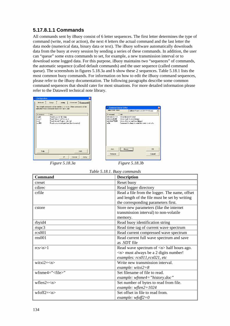
134

5.17.8.1.1 Commands All commands sent by iBuoy consist of 6 letter sequences. The first letter determines the type of command (write, read or action), the next 4 letters the actual command and the last letter the data mode (numerical data, binary data or text). The iBuoy software automatically downloads data from the buoy at every session by sending a series of these commands. In addition, the user can “queue” some extra commands to set, for example, a new transmission interval or to download some logged data. For this purpose, iBuoy maintains two “sequences” of commands, the automatic sequence (called default commands) and the user sequence (called command queue). The screenshots in figures 5.18.3a and b show these 2 sequences. Table 5.18.1 lists the most common buoy commands. For information on how to edit the iBuoy command sequences, please refer to the iBuoy documentation. The following paragraphs describe some common command sequences that should cater for most situations. For more detailed information please refer to the Datawell technical note library.

Figure 5.18.3a Figure 5.18.3b

Table 5.18.1. Buoy commands Command Description creset Reset buoy cdirec Read logger directory crfile Read a file from the logger. The name, offset

and length of the file must be set by writing the corresponding parameters first.

cstore Store new parameters (like the internet transmission interval) to non-volatile memory.

rbyid4 Read buoy identification string rtspc3 Read time tag of current wave spectrum rcs001 Read current compressed wave spectrum rns001 Read current full wave spectrum and save

as .SDT file rcs<n>1 Read wave spectrum of <n> half hours ago.

<n> must always be a 2 digits number! examples: rcs011,rcs021, etc

witxi2=<n> Write new transmission interval. example: witxi2=8

wfnme4=”<file>” Set filename of file to read. example: wfnme4=”history.doc”

wflen2=<n> Set number of bytes to read from file. example: wflen2=1024

wfoff2=<n> Set offset in file to read from. example: wfoff2=0

135

5.17.8.1.2 Default command examples Here follow some example default command sequences Downloading of current full wave spectrum This sequence will download the current full spectra and save it as an .SDT file. Only the current full spectrum can be downloaded. This list can be used with any transmission interval. rbyid4 (read buoy identification) rtspc3 (read time tag of last spectrum) ritxi2 (read transmission interval) rns001 (read current full wave spectrum) Downloading of current full wave spectrum and compressed wave spectrum This sequence is identical in function to the above sequence but also downloads the current compressed wave spectrum. This is useful when iBuoy is used with a live connection to W@ves21. This way, the real-time display of W@ves21 will automatically be updated. rbyid4 (read buoy identification) rtspc3 (read time tag of last spectrum) ritxi2 (read transmission interval) rcs001 (read current compressed wave spectrum) rns001 (read current full wave spectrum) Downloading of last 2 to 12 compressed wave spectra This sequence is used when the transmission interval is set to 2 or higher. In this case, it is desirable to not only download the current wave spectrum but all new wave spectra since the previous session. This is done by sending multiple read commands as shown in the following command sequence: rbyid4 (read buoy identification) rtspc3 (read time tag of last spectrum) ritxi2 (read transmission interval) rcs<n>1 (read compressed spectrum of <n> half hours ago) rcs021 (read compressed spectrum of 2 half hours ago) rcs011 (read compressed spectrum of 1 half hour ago) rcs001 (read current compressed spectrum) Depending on the chosen interval, you can download up to 12 compressed wave spectra during a single session.

5.17.8.1.3 User command examples Here follow some example command sequences which can be queued by the user. Setting a new transmission interval This sequence will set the transmission interval to its maximum value of once every half hour. The cstore command assures the new setting will survive a buoy reset. Other transmission intervals can be set by changing the value of witxi2. witxi2=1 (set interval to 1*half hour) cstore (store new settings)

136

Downloading spectral data from the logger This sequence will download an .SDT file from the internal logger. SDT files can contain up to 1488 full wave spectra. To save transmission time, it is therefore necessary to download only the section of the file that is of interest. This is done by calculating an offset into the file and the length of the file section to download. In this example, data from the 19th of May 2006 is downloaded. For the precise structure of the logger files, please refer to the Datawell technical note library. wfnme4=”S05-2006.SDT” (file with spectral data of May 2006) wflen2=26688 (length = 48 spectra of 556 bytes) wfoff2=480384 (offset = 18 days * 48 spectra of 556 bytes) crfile (read actual data) Downloading history.doc from the logger This sequence will download the history file “history.doc” from the internal logger. It is assumed that the file is less than 99999 bytes long (for longer files, wflen2 may be increased or only the last few kilobytes of the file may be downloaded). wfnme4=”HISTORY.DOC” (history file) wflen2=99999 (length = long enough) wfoff2=0 (download from beginning of file) crfile (read actual data)

5.18.8.2 Waves4-configurator The communication with the buoy is handled by the Waves4-configurator. Please refer to the Waves4 Operator Manual for setting up the Waves4-configurator correctly. The Waves4-configurator is a very flexible piece of software and allows you to remotely request all available DMF messages as well as data stored on the CF-card. Furthermore, it is also possible to remotely change the settings of the dial script, destination host and port, transmission interval etc. if necessary.

5.17.8.2.1 First time setup As explained in previous chapter, the buoy can be configured remotely using the Waves4-configurator. However, the first time setup needs to be performed using the console of the hatchcover. The buoy needs to be configured first before it is able to transmit the message data at specific intervals to the specified hostname/IP address. You will have to do this only once. After powering up the buoy, it will connect to the Iridium satellites (or GSM network) and try to set-up a connection with the specified hostname/IP address. Once connected, the buoyd service will send a message to the buoy containing the requested DMF messages, interval and offset. The settings are stored in the EEPROM so power-down or reset will not affect the interval settings. With the forcetcp console command you can initiate a connection outside the programmed intervals. This command is generally used for testing purposes. General note: Without a GPS position and time fix, e.g. when testing in-doors, the Iridium-internet and GSM-internet transmission will be referred to the internal buoy time instead of UTC. As a consequence the timing of the internet connection will not occur on the expected UTC times. Be aware of the fact that during the in-door testing of the buoy the system will have no clear view of the sky and therefore cannot communicate with the Iridium satellites. This will not only prevent Iridium-internet communication, it may also increase the buoys energy consumption, depending on the chosen transmission interval.

137

5.18.8.3 Error messages The buoy can give out a number of error numbers related to internet communication. The error numbers are printed out through the console and logged on the internal data logger. The error numbers are given in the form “TCP: error:<N>”, where <N> is the error number. This section discusses all error numbers, their meaning and a possible cause or solution.

Table 5.18.2. Error numbers

Error meaning cause / solution 1 dialling failed Caused by bad signal and/or wrong dial script. Check that the

SIM card is properly installed and has no PIN code enabled. Also check if the antenna has a clear view of the sky (in case of Iridium) and that the dial script has been correctly entered

2 ppp failed Caused by bad signal and/or wrong dial script. Check that the SIM card is properly installed, the antenna has a clear view of the sky (in case of Iridium) and that the dial script has been correctly entered. (especially dial number, username and password)

3 internal error Firmware failure, please contact Datawell. 4 host not found Only occurs when a non-existent domain hostname has been

entered. Enter the correct domain hostname or enter a straight IP address.

5 connection failed The destination host is not responding. Please check the destination computer firewall settings and make sure that iBuoy is correctly configured and running.

6 tcp/ip error Internet communication error. Happens sometimes due to bad signal. Check if the antenna is in good condition and if the antenna has a clear view of the sky (in case of Iridium).

7 tcp/ip error Internet communication error. Happens sometimes due to bad signal. Check if the antenna is in good condition and if the antenna has a clear view of the sky (in case of Iridium).

8 no dns server The ISP did not provide a valid DNS (domain name server) server. If this is the case domain host names cannot be used. Consider entering a straight IP address.

9 tcp/ip error or connection failed

Internet communication error. Happens sometimes due to bad signal. Check if the antenna is in good condition and if the antenna has a clear view of the sky (in case of Iridium). This error can also occur if the destination host is not responding. See error 5 for more information.

138

GPRS communication 5.18.9Please refer to chapter 5.17.1 Internet communication for setting up the buoy correctly and use this chapter for additional information which is important in case you want to use the GPRS connection of the GSM communication link. Waverider buoys may be fitted with a GSM link, transmitting data across the internet. In the previous chapters several examples are given on how to set up a dial-in connection. However, some mobile networks have discontinued their dial-in service. It has been replaced by GPRS and later technologies. To keep up the data link your buoy GSM configuration must be modified to set up a GPRS connection. Even without this necessity switching to GPRS may be motivated by the lower cost.

GPRS versus GSM dial-in 5.18.10GSM connections are mostly used for speech. The acoustic signals are converted to packets. GPRS is short for General Packet Radio Service, in this case packets of data. The same GSM network is used and often the same GSM modem can be used. As a result network coverage on your buoy location and performance in your typical wave conditions remains identical. However, there is one important difference: GPRS has lower priority than speech (dial-in).

Compatible GSM modems 5.18.11To find out if your GSM modem supports GPRS please check the manufacturer and model with help of the photographs. uBlox LISA modems, Telit modems and Siemens modems MC55 and MC55i are compatible with GPRS communication, but Siemens modem TC35i is not although it can be replaced with a MC55(i) modem. Please contact Datawell Service.

Setting up a GPRS connection 5.18.12The GSM link can be configured locally via a settcp command over the console (see chapter 5.17.1). Dial-script commands, internet-address and -port, etc must be set for the primary and secondary connection. To switch to GPRS mainly the dial-script must be changed. The GPRS dial-script template is as follows: where AT+CGDCONT and AT+CGDATA are specific GPRS commands that replace the ATD command of the dial-in template. If a connection fails, extend the waiting period by replacing d10s with d20s. This will give the modem more time to log on to the network. Verify that the provider approves logging on to different networks. This can become an issue if a buoy is drifting away from its original location. While still supported, you can configure the secondary (backup) script for standard GSM dial-in connection. The second script will be used if the first script fails. Important: Warning In principle the GSM link can be configured remotely, but experimenting with a buoy out at sea is not recommended.

d10sAT&F#~sAT&K0#~sAT+CGDCONT=1,"IP","<APN>"#~sAT+CGDATA="PPP",1#~w60CONNECT~p<Login>,<Password>~

139

Copyright 5.18.13The Datawell internet communication module uses the UIP TCP/IP stack. Copyright (c) 2001-2006, Adam Dunkels and the Swedish Institute of Computer Science All rights reserved. Redistribution and use in source and binary forms, with or without modification, are permitted provided that the following conditions are met: 1. Redistributions of source code must retain the above copyright notice, this list of conditions and the following disclaimer. 2. Redistributions in binary form must reproduce the above copyright notice, this list of conditions and the following disclaimer in the documentation and/or other materials provided with the distribution. 3. The name of the author may not be used to endorse or promote products derived from this software without specific prior written permission. THIS SOFTWARE IS PROVIDED BY THE AUTHOR `AS IS' AND ANY EXPRESS OR IMPLIED WARRANTIES, INCLUDING, BUT NOT LIMITED TO, THE IMPLIED WARRANTIES OF MERCHANTABILITY AND FITNESS FOR A PARTICULAR PURPOSE ARE DISCLAIMED. IN NO EVENT SHALL THE AUTHOR BE LIABLE FOR ANY DIRECT, INDIRECT, INCIDENTAL, SPECIAL, EXEMPLARY, OR CONSEQUENTIAL DAMAGES (INCLUDING, BUT NOT LIMITED TO, PROCUREMENT OF SUBSTITUTE GOODS OR SERVICES; LOSS OF USE, DATA, OR PROFITS; OR BUSINESS INTERRUPTION) HOWEVER CAUSED AND ON ANY THEORY OF LIABILITY, WHETHER IN CONTRACT, STRICT LIABILITY, OR TORT (INCLUDING NEGLIGENCE OR OTHERWISE) ARISING IN ANY WAY OUT OF THE USE OF THIS SOFTWARE, EVEN IF ADVISED OF THE POSSIBILITY OF SUCH DAMAGE.

140

5.19 GSM-SMS communication The GSM communication link is optional on Datawell wave buoys. It is offered as an alternative to the HF-link for near shore applications, 10 Km typically. Wave spectra, meteorological parameters, buoy information and other messages can be sent from any location to any location within the reach of the GSM network. This section will describe how to install and operate the buoy side of the GSM-SMS link. A separate manual is devoted to the receiving side, i.e. GSM modem and gsmBuoy Windows software. Contact Datawell Sales to obtain a copy.

Enabling the GSM option 5.19.1For more detailed information about the steps below read the corresponding paragraphs

- Choose a GSM network provider with the best GSM coverage at the measuring location. - Prepare the SIM card, so it can be used without PIN-code protection. - Install the SIM card in the GSM modem of the buoy - Connect the electronics unit to the batteries/hull. - Close the buoy (make sure that the rubber sealing ring is placed). - Attach the GSM antenna to the hatch (make sure that the rubber sealing ring is placed). - Place the buoy outside at a location where it can receive GPS signals. - Configure the GSM-link mode of operation using a PC + GSM modem and gsmBuoy

Windows software. The GSM-link is default configured to sleep-mode. For testing you can configure to active-mode. After testing please reconfigure to sleep-mode to save energy.

- When the buoy responds with a confirmation message, the GSM link is setup correctly.

Disabling the GSM option 5.19.2When the installed GSM option is not required it MUST be disabled by using the setconfig command using the console port of the electronics unit. Removal of the SIM-card in order to disable the GSM option is NOT the correct method to disable the GSM option.

Choosing a GSM network provider 5.19.3The GSM-option requires the services of a GSM network provider in order to use the GSM network infrastructure. Although there are probably multiple GSM network providers in your area not all providers are suited for the use of the GSM-option. In order for the GSM-link to function best a GSM network with the best coverage, in the area where the buoy is deployed, should be chosen. The difference between good and bad coverage is shown below.

Figure 5.19.1. GSM network coverage of two different providers in The Netherlands. (a) on the

left, poor GSM network coverage at sea, (b) on the right, better coverage at sea.

141

Figure 5.19.1(a) shows GSM network coverage near the coastline but only very close to the coastline, whereas Figure 5.19.1(b) shows a GSM network coverage that reaches for many kilometres out of the coastline. Therefore the GSM network provider of Figure 5.19.1(b) is best used since a better coverage ensures a higher reliability of our GSM-option. For coverage maps of other countries visit the website of “GSM world” at: http://www.gsmworld.com/roaming/gsminfo/index.shtml. Select the country in which the buoy is to be deployed and choose “coverage map” and/or “network information”. When selecting a GSM network provider also make sure that the GSM network is capable of supporting the following frequency standards (this can be checked under “network information”): (E)GSM900, GSM 1800 and GSM1900 When a good network provider has been found, go to your local telecommunications store and purchase a subscription to gain access to the required GSM network.

Attention regarding prepaid SIM-cards 5.19.4Although the prepaid SIM-card looks promising, because it is cheap and easy obtainable, it may be a problem to upgrade the prepaid value or credits. Because most prepaid SIM-cards require a 6 or 12 month upgrade of the prepaid value by a certain amount in order to maintain the connection to the GSM network provider. And because it is not possible to recharge a prepaid SIM-card remotely it may become a problem for buoys that send a lot of SMS’s over a great length of time. When the prepaid value has decreased to zero or expires, your buoy is not capable of sending data over the GSM-link and may become useless unless serviced. I.e. it must be retrieved to recharge the prepaid SIM-card. Therefore a SIM-card with subscription is strongly recommended for use in buoys.

Preparing and installing the SIM-card 5.19.5In order for the GSM-option to function properly a SIM-card must be installed. Since the GSM-option uses the GSM infrastructure it requires the proper licenses in the form of a SIM-card. This SIM-card is identical to the SIM-card in your own GSM phone. It may be a prepaid or a subscription (preferred) SIM-card. The SIM-card of your GSM network provider is supplied with a PIN-code, this is an identification code of maximally 8 digits, for example 0000 or 1234. In addition it has a PUK-code, this is an identification code of maximally 8 digits, this PUK-code is unique and required when the PIN-code has been entered incorrectly for 3 times. Carefully write these numbers down and store them in a safe place for later use. In order for the GSM-option to function, the SIM-card used has to be in unprotected mode: a mode where the SIM-card does not require a PIN- or PUK-code. Default SIM-cards require a PIN- or PUK-code, but they can be configured to an unprotected mode by the use of the Datawell GSM-buoy software or an ordinary GSM mobile phone. For setting the SIM-card to unprotected mode, with help of the Datawell GSM-buoy software, refer to the GSM-buoy software manual. To set the SIM-card to unprotected mode using a GSM mobile phone, see the example below. Example. Converting PIN-protected SIM-card to unprotected SIM-card using the Nokia 3310: Menu Settings Security settings PIN code request Enter PIN code (enter current PIN-code) Off

142

Now the SIM-card is configured as an unprotected SIM-card. This setting is stored on the card itself and can be changed back to protected mode when required. To install the SIM-card into the GSM modem, open the electronics unit. The GSM modem is easily accessible and located on the GSM printed circuit board. Datawell uses the uBlox LISA GSM modem. Before installing the SIM-card, first power off the electronics unit. Then gently insert the SIM-card in the right direction according to the drawing on top of the modem, see Figure 5.19.2. Press the SIM-card in the modem until it locks. To remove the SIM-card from the modem, press it so that it will unlock.

Figure 5.19.2. Installing the SIM-card in the GSM modem in the FB2 electronics unit.

GSM configuration and command message 5.19.6 Configuration Depending on the configuration, the buoy will send its data every 30min, 1 hour, 2 hours or 3 hours (from the time the buoy was switched on). New configurations can be send from the destination receiver (PC with GSM modem) to the buoy at any time. Depending on the mode of operation it may take up to 3 hours before the buoy responds with a confirmation of the new settings. The response time is smallest when the buoy is in the active-mode (in this mode the GSM receiver will be continuously switched on and therefore consumes more energy than when in sleep-mode). The response time is largest when the buoy is in sleep mode with a 3 hour transmission interval, since the GSM-link will power down when not transmitting it is not capable of receiving a new configuration message outside the transmission period. Therefore the first possible moment that the configuration message will be received is directly after the transmission of data. The sleep-mode is the preferred mode as it consumes the least amount of energy. Therefore this is also the default setting. A Waverider buoy with GSM-option requires two configuration settings in order to function. Required settings are: transmission interval and power-mode. Both settings can be configured with the Datawell gsmBuoy software. In fact the software will send an SMS text-command message as follows buoy-config <transmission-interval> <power-mode>

143

where <transmission-interval> = 30min, 1hr, 2hr or 3hr <power-mode> = sleep or active The example below shows how to configure the buoy to a 30 minute transmission interval combined with the power-mode sleep. This means that the GSM link is switched off between transmissions. buoy-config 30min sleep The origin (or sender) of the configuration message determines the destination of the data messages the buoy will send. In other words: when the buoy receives the buoy-config command, it will change the destination address (telephone number) into the telephone number of the GSM-modem that sent the buoy-config command. This way the destination address will always be correct after sending the configuration message. Status request command Sometimes it may be desirable to request the status of the buoy or its GSM-link when you are not near the receiver unit. For example, to check the functionality of the GSM-link shortly after deployment. In this case an ordinary GSM mobile phone (capable of sending SMS messages) can be used. This command does not affect the configuration in any way. The example below shows how to request the buoy-status. Sending the following SMS to the GSM number of the buoy: buoy-status The buoy will reply to the sender of this command (within 2min. to 3 hours) depending on the operation mode with a status SMS message. This message is a normal SMS message that can be viewed on the GSM mobile phone the buoy-status SMS was sent from. The example below shows a status message received from a buoy.

Buoy-status: Lat:unknown Lon:unknown Pwr=0.9W at 11.0V Rlfe=0Wks Hs=0.00m Tz=0.0s Tsea=-273.1C Rlvl min:-85dB, avr:-83dB max:-79dB

Lat: unknown no GPS position (latitude) determined (longitude idem) Pwr=0.9W measured buoy energy consumption 0.9 Watt at 11.0V measured battery voltage is 11.0 Volt Rlfe=0Wks remaining life span of battery is 0 weeks (batteries are exhausted) Hs=0.00m significant wave height of 0.00 m Tz=0.0s zero up cross period 0.0 s Tsea=-273.1C sea water temperature could not be determined (absolute zero temp) Rlvl min:-85dB minimum reception level of GSM network avr:-83dB average reception level of GSM network max:-79dB maximum reception level of GSM network

Note: the min/avr/max reception levels are measured over a period of 2 minutes (the average value is calculated over 100 measurements). These measurements will be executed directly after receiving the buoy-status message.

144

Data message 5.19.7Data message is transferred in SMS PDU-mode and cannot be displayed as readable text. The PDU-mode is a standardized mode of sending data over SMS and is described in the AT-command manual of the GSM-modem used. The message itself consists of set of concatenated standard Datawell messages preceded by a message identification header: Message identification header 305D Compressed heave-spectrum <31 bytes> Compressed directional-spectrum <31 bytes> Spectral parameters <11 bytes> Buoy information <10 bytes> Sea surface temperature <10 bytes> Air temperature <10 bytes> For a detailed description of the individual messages refer to subsection 5.7.2 “Datawell message format”.

Power consumption 5.19.8Power consumption of the GSM module depends on the configuration of the GSM-module. Table 5.19.1 below shows the average power consumption of the GSM-link for different configurations. Power consumption values are indicative as the actual power consumption also depends on distance to the nearest GSM network antenna, wave and weather conditions, background noise, etc.

Table 5.19.1. Average power consumption for all configurations. Transmission

interval Power mode

ON-time Average power consumption (mW)

GSM mode

every 30 min sleep 10% 60 0x00 every 1 hour sleep 5% 30 0x01 every 2 hours sleep 2.5% 15 0x03 every 3 hours sleep 1.6% 10 0x05 every 30 min active 100% 300 0x10 every 1 hour active 100% 275 0x11 every 2 hours active 100% 265 0x13 every 3 hours active 100% 255 0x15 disabled (0% ON) (console configuration, cannot be set remotely) 0xFF

The power-mode “active” is mainly to be used for testing purposes; it enables a quicker response time to configuration messages and status requests but consumes more power. The GSM mode (last column) can be requested via the console using the showconfig command, which would return the following (example): Installed battery capacity: 12150 Wh RF link: disabled

Gsm mode: 0x05 (sleep) GSM destination: +31612345678 This means that the transmission interval is every 3 hours and the power mode is sleep.

145

GSM antenna 5.19.9The GSM antenna is designed for the GSM radio bands: 850, 900, 1800 and 1900 MHz. For transportation the GSM antenna is removed from its port and packed inside the buoy. The GSM antenna should be mounted on the GSM port on the hatchcover. Please make sure the rubber sealing ring is in place when mounting the antenna.

Figure 5.19.3 GSM antenna

Specifications 5.19.10Table 5.19.2 summarizes some important GSM specifications.

Table 5.19.2. GSM modem and GSM option specifications.

Parameter Specification GSM modem (uBlox LISA)

Frequency band Quad-band, GSM850, EGSM900, GSM1800 and GSM1900

Output power Class 4 (2 W) EGSM900 Class 1 (1 W) GSM1800 Class 1 (1W) GSM1900

Approvals R&TTE GCF approval

SIM card prepaid mini-SIM card subscription mini-SIM card

GSM option Power consumption

8 mW - 110 mW depending on operation mode

Transmission range

10 Km typical (line of sight), depending on network coverage and performance

Supported format Datawell message format (transmission over SMS in PDU format)

146

5.20 Iridium-internet satellite communication Iridium is a satellite based cellular phone network. It is built upon a constellation of 66 low earth orbit (LEO) satellites. The constellation is organized in such a way that every part of the globe is covered 24 hrs a day. Iridium gets its name from the element Iridium (Ir), which has an atomic number of 77. This name was chosen because the constellation would initially be built upon 77 satellites. The Datawell Iridium option makes it possible to send spectral data and raw displacement data directly over the internet to a computer running W@ves21. The Iridium option consists of an Iridium satellite modem that fits in the electronics unit and an Iridium antenna. Please refer to chapter 5.17.1 Internet communication for setting up the buoy correctly.

Antenna 5.20.1The Iridium option uses a special antenna. The antenna is similar in design to the GPS position antenna but it has a different colour. Whereas the GPS antenna is yellow, the Iridium antenna is black. The Iridium antenna is mounted in the unlabelled option port. When mounting the antenna, always check if the rubber sealing ring is present and if the sealing ring contact surfaces are clean. When testing the buoy on shore, make sure the antenna has a clear and unobstructed view of the sky and avoid tall buildings and trees in the direct vicinity of the buoy. As the Iridium satellites are in a low earth orbit (LEO) they are often seen by the buoy at relatively small angles. Therefore, it is important that the buoy has a broad view of the sky hence avoid tall buildings and trees.

Satellite modem 5.20.2The Datawell Iridium-internet option uses a 9523 Iridium L-band transceiver. This modem is built into the electronics unit. To power the modem, a dedicated power supply is also integrated into the electronics unit on the same printed circuit board as the modem. The antenna connector and the SIM-card bracket of the modem are accessible after removing the lid from the electronics unit.

SIM-card 5.20.3Since the modem uses the Iridium network, an Iridium subscription is necessary. To identify the Iridium subscriber on the network, a SIM-card is used (supplied by your local provider). The Iridium modem is located on the iridium printed circuit board inside the electronics unit. Make sure the electronics unit is switched off. The SIM card can easily be installed in the SIM card holder. Please refer to figure 5.20.1. The SIM card holder uses a push-push system to insert and remove the SIM card. With an extra lock mechanism you are sure the SIM card is well installed during operation.

147

Figure 5.20.1 Schematic overview of SIM-card installation

PIN-code 5.20.4In order for the Iridium option to function, the SIM-card has to be in unprotected mode: a mode where the SIM-card does not require a PIN- or PUK-code. Please indicate this to the Iridium provider when ordering a SIM-card. The provider should be able to deliver an unprotected SIM-card. If the SIM-card is not in unprotected mode, the PIN-code has to be removed. Please contact your Internet Service Provider.

Configuration and operation 5.20.5The Iridium option is designed to operate with the internet communication software of the buoy. Please refer to chapter 5.18 (GSM-internet) for more information.

Specifications 5.20.6Table 5.20.1 summarizes some important Iridium specifications.

Table 5.20.1. Iridium specifications HF Frequency band 1616 – 1626.5 MHZ

Transmit power 7 W max. Power consumption

Minimum 6 mW (1 update / day) Typical 16 mW (8 updates / day) Maximum 74 mW (48 updates / day)

Communication Data format Datawell internet communication / iBuoy

148

5.21 Iridium-SBD satellite communication

Iridium satellite system 5.21.1Please refer to section 5.20 Iridium internet satellite communication for an introduction to the Iridium satellite system.

Iridium SBD service and email 5.21.2Iridium offers a number of services, one of which is Iridium Short Burst Data (SBD). Iridium SBD communicates data via short messages, much the same as GSM text messages (SMS). Messages originating from the Iridium SBD modem are limited to 340 bytes and messages terminating at the modem are limited to 270 bytes. The user interface consists of an arbitrary email program. To get acquainted with the Iridium SBD message format, the example of the incoming email is illustrative, see Figure 5.21.1. Most of the fields are fixed and self-explanatory, but some require more explanation. IMEI-number A Waverider buoy with Iridium SBD cannot be identified by the fixed 'from'-email-address. However, every Iridium SBD modem has a unique hard-coded number: the IMEI number, International Mobile Equipment Identification number. Also every cell-phone carries such an IMEI-number. The SBD modem IMEI-number is listed in the subject-field. There are several ways to obtain the IMEI number. The number is printed on the PCB of the Iridium modem installed in the hatch. Alternatively, the IMEI number will be outputted by the buoy after start-up. Connect a laptop/PC to the console of the hatchcover to obtain the IMEI number. Or you can contact our sales department (sales@datawell.nl). ´To´-email-address Best is to use a dedicated email account for the sbdBuoy software (refer to chapter 5.21.6). If the SBD messages are sent to a personal email account, the SBD messages would mix with your personal messages. Although the sbdBuoy program will not interfere with your personal messages, outlook (or any other email program) will remove all messages from the inbox of the email server. This makes it impossible for the sbdBuoy program to receive any SBD related messages. Message numbers The Iridium SBD service logs two message numbers MOMSN and MTMSN, where MO: mobile originated (data from buoy to user) MT: mobile terminated (command from user to buoy) Both numbers roll over at 216 = 65536, i.e. after 3.7 years at ½ hour message intervals. The attachment filename is made up of the IMEI- and MOMSN-numbers. Messages are time-tagged and buoys are identified by the Iridium SBD modem's IMEI-number. Furthermore, each message contains a global position estimate. CEP, short for Circular Error Probability, is expressed in km. Position accuracy is typically a few km’s. This is the position based on a Doppler and time delay measurement by the Iridium system, not on the GPS measurement of the buoy.

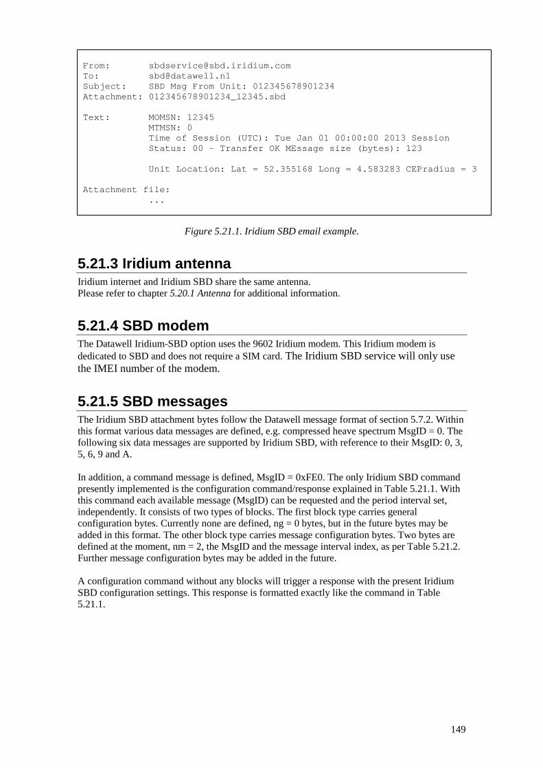
149

From: sbdservice@sbd.iridium.com To: sbd@datawell.nl Subject: SBD Msg From Unit: 012345678901234 Attachment: 012345678901234_12345.sbd Text: MOMSN: 12345 MTMSN: 0 Time of Session (UTC): Tue Jan 01 00:00:00 2013 Session Status: 00 - Transfer OK MEssage size (bytes): 123 Unit Location: Lat = 52.355168 Long = 4.583283 CEPradius = 3 Attachment file: ...

Figure 5.21.1. Iridium SBD email example.

Iridium antenna 5.21.3Iridium internet and Iridium SBD share the same antenna. Please refer to chapter 5.20.1 Antenna for additional information.

SBD modem 5.21.4The Datawell Iridium-SBD option uses the 9602 Iridium modem. This Iridium modem is dedicated to SBD and does not require a SIM card. The Iridium SBD service will only use the IMEI number of the modem.

SBD messages 5.21.5The Iridium SBD attachment bytes follow the Datawell message format of section 5.7.2. Within this format various data messages are defined, e.g. compressed heave spectrum MsgID = 0. The following six data messages are supported by Iridium SBD, with reference to their MsgID: 0, 3, 5, 6, 9 and A. In addition, a command message is defined, MsgID = 0xFE0. The only Iridium SBD command presently implemented is the configuration command/response explained in Table 5.21.1. With this command each available message (MsgID) can be requested and the period interval set, independently. It consists of two types of blocks. The first block type carries general configuration bytes. Currently none are defined, ng = 0 bytes, but in the future bytes may be added in this format. The other block type carries message configuration bytes. Two bytes are defined at the moment, nm = 2, the MsgID and the message interval index, as per Table 5.21.2. Further message configuration bytes may be added in the future. A configuration command without any blocks will trigger a response with the present Iridium SBD configuration settings. This response is formatted exactly like the command in Table 5.21.1.

150

Table 5.21.1. Iridium SBD, configuration command and response message. Field Value Description

TaskID 96 Iridium SBD task CmdID 1 Configuration

command/response

Cmd length n variable Cmd byte 0 ng = 0 number of general

configuration bytes

1 nm = 2 number of MsgID configuration block bytes

1+(1..ng) (future general configuration block)

1+ng+(1..nm) first MsgID configuration block

byte 1: MsgID 2: message interval according to index, Table 5.21.2. future MsgID configuration bytes

1+ng+nm+(1..nm) next MsgID configuration block

… n−nm−1+(1..nm) last MsgID configuraion

blocks

Table 5.21.2 maps the message interval index to the message interval. Requesting a message once, index 0, will terminate transmission of that particular message after that one time. Indices 11-254 will be interpreted as index 10. Index 255 will disable the particular message identified by MsgID in byte 1. Even when all messages are disabled, the buoy will check the SBD inbox every day at midnight (UTC). Table 5.21.3 outlines all message intervals and their corresponding time of transmission. The Iridium SBD system will try once and then retry three times to establish a connection. If still no connection could be made, the scheduled messages are lost. The buoy will no longer attempt transmission until the next transmission interval.

Table 5.21.2. Message interval index table.

Index Message interval (hour:min)

Frequency (messages per day)

0 - once 1 24:00 1 2 12:00 2 3 8:00 3 4 6:00 4 5 4:00 6 6 3:00 8 7 2:00 12 8 1:30 16 9 1:00 24 10 0:30 48 255 - disable message

151

Table 5.21.3. Message intervals and corresponding transmission time Transmission interval

Transmission time (UTC) (+30 min. max.)

0 (once)

1 (24:00)

2 (12:00)

3 (8:00)

4 (6:00)

5 (4:00)

6 (3:00)

7 (2:00)

8 (1:30)

9 (1:00)

10 (0:30)

00:00 ? √ √ √ √ √ √ √ √ √ √ 00:30 ? √ 01:00 ? √ √ 01:30 ? √ √ 02:00 ? √ √ √ 02:30 ? √ 03:00 ? √ √ √ √ 03:30 ? √ 04:00 ? √ √ √ √ 04:30 ? √ √ 05:00 ? √ √ 05:30 ? √ 06:00 ? √ √ √ √ √ √ 06:30 ? √ 07:00 ? √ √ 07:30 ? √ √ 08:00 ? √ √ √ √ √ 08:30 ? √ 09:00 ? √ √ √ √ 09:30 ? √ 10:00 ? √ √ √ 10:30 ? √ √ 11:00 ? √ √ 11:30 ? √ 12:00 ? √ √ √ √ √ √ √ √ 12:30 ? √ 13:00 ? √ √ 13:30 ? √ √ 14:00 ? √ √ √ 14:30 ? √ 15:00 ? √ √ √ √ 15:30 ? √ 16:00 ? √ √ √ √ √ 16:30 ? √ √ 17:00 ? √ √ 17:30 ? √ 18:00 ? √ √ √ √ √ √ 18:30 ? √ 19:00 ? √ √ 19:30 ? √ √ 20:00 ? √ √ √ √ 20:30 ? √ 21:00 ? √ √ √ √ 21:30 ? √ 22:00 ? √ √ √ 22:30 ? √ √ 23:00 ? √ √ 23:30 ? √ Note: “only once” messages will be sent directly after the request (configuration message) has been received. Configuration messages are received after every transmission or at 0:00 (UTC).

152

Software 5.21.6The above explanation allows customers to compose Iridium SBD configuration command messages and translate response and data messages. Alternatively customers can also use the Datawell sbdBuoy or Waves4-configurator software (recommended).

5.21.6.1 sbdBuoy It offers menu-based configuration command editing and email data handling and storage. It integrates with W@ves21 for further data processing and presentation. A single program can deal with a network of Waverider buoys equipped with Iridium SBD. Furthermore, the PC does not have to be permanently on-line or permanently powered since emails will be buffered by the internet provider. As explained earlier, it is preferred to use a dedicated email account for the sbdBuoy software. Note: Make sure the regional settings of your computer use the point (.) as decimal symbol. Otherwise the received spectral files (WFT) will not be displayed correctly in W@ves21.

5.21.6.2 Waves4-configurator The Waves4 software supports the storage, processing and presentation of received Iridium SBD emails, as well as composing configuration emails. It can deal with a network of Waverider buoys equipped with Iridium SBD. Furthermore, the PC does not have to be permanently on-line or permanently powered since emails will be buffered by the internet provider. As explained earlier, it is preferred to use a dedicated email account. A single account suffices for a network of Iridium SBD buoys. Please refer to the Waves4 operator and user manual for more information.

First time setup 5.21.7The buoy settings can only be configured using the software. It is not possible to configure the buoy using the console. Therefore it is advisable to send a configuration message prior to powering the buoy. After powering up the buoy, it will connect to the Iridium satellites and check the inbox for configuration messages. If you have already sent a configuration message, the new configuration will take effect immediately. The settings are stored in EEPROM so power-down or reset won’t affect the interval settings. It is not possible to contact the buoy outside the programmed intervals. If no messages are requested, the buoy will still call in once per day, Midnight UTC, to allow the user to change the settings. Furthermore, when starting the buoy Iridium SBD message timing is referenced to the time since power-up. After the first GPS position and time fix, Iridium SBD message timing is referenced to UTC time. To monitor the functionality of the Iridium SBD system you need to connect to the console of the hatch. With the startdebug command you can set the console into the debug mode. In this mode the hatch outputs more information about the current state of the hatch. During the transmission of SBD messages you’ll see messages that indicate if a SBD transmission was successful or not. Also when the SBD related software receives a configuration message or encounters an error or time-out situation, it will add information to the HISTORY.DOC on the CF-card.

153

Specifications 5.21.8

Table 5.21.4. Iridium SBD specifications HF Frequency band 1616 – 1626.5 MHZ

Transmit power 1.6 W max. Energy consumption

Maximum 50 mW (48 updates / day)

Communication Data format sbdBuoy

The number of DMF messages per SBD email, i.e. the number of bytes has negligible effect on the energy consumption. Energy consumption will be proportionally lower for longer message intervals.

154

5.22 Argos satellite communication Argos is a satellite communication system operated by CLS (Collecte Localisation Satellites). CLS can be contacted at www.cls.fr. Argos satellite communication on Datawell buoys is optimized for two purposes. One is to track a buoy adrift (position); the other application is for communicating basic wave information from remote locations on the sea (data). Before deploying the buoy, the Argos antenna must be installed and the operating mode must be set. Refer to chapter 5.22.1 for Argos antenna installation instructions and chapter 5.22.2 for instructions on setting the Argos operating mode.

Installing the Argos antenna 5.22.1Argos needs a dedicated antenna.. For general antenna installation instructions, refer to paragraph 5.3.6. Figure 5.22.1(a) shows the orientation of the Argos antenna on the hull. The ground plane radials are fixed to the main antenna using a single hexagon socket screw, see figure 5.22.1(b). The ground plane radials are necessary for correct operation of the Argos antenna.

Figure 5.22.1. Orientation of the Argos antenna(a), Argos antenna radials(b).

155

Setting the Argos operating mode 5.22.2As Argos is a one-way communication system (Argos can only communicate data from the buoy to the user), the operating mode has to be set prior to deployment. The operating mode is set using the setconfig console command (refer to chapter 5.11.4). The operating modes are summarized in table 5.22.1. There are four possible operating modes: • Mode 0 disables the Argos module. In this mode, no power is consumed by the Argos

module. • Modes 1 and 2 are the so-called “classic” modes. These modes are identical to the modes

available in the older MkI and MkII Directional Waveriders. • Mode 3 is the default (and recommended) operating mode. This mode is fully supported by

the CLS ArgosWeb data collection system, supports 28bit ID’s, provides all basic wave parameters and delivers accurate GPS-class positions.

• Mode 4 is identical to mode 3 but adds a power spectrum of the collected wave data.

Table 5.22.1. Argos operating modes.

Description of Argos operating modes 5.22.3The possible Argos modes differ in several aspects like data format and position accuracy. The paragraphs below discuss these aspects.

Compatibility with 28BIT ID’s 5.22.4Modes 1, 3 and 4 are compatible with both the newer 28bit ID’s and the classic 20bit ID’s. Mode 2 is only compatible with classic 20bit ID’s. Therefore, if mode 2 is desired, please indicate the preference for a 20bit ID when applying for a new ID at CLS.

Position accuracy 5.22.5There are two ways of determining the buoy position; Doppler and GPS. Doppler is used by mode 1 and 2. With Doppler, the position of the buoy is determined by the Argos satellite itself as it passes over the buoy. Doppler positions have an average accuracy of 350m. GPS is used by modes 3 and 4. With GPS, the position of the buoy is determined by the GPS receiver of the buoy. This position is sent to the ARGOS satellite. GPS positions have an average accuracy of 10m.

MODE 28BIT ID POSITION DATA 0 Argos module disabled 1 yes Doppler n/a 2 no Doppler compressed wave spectrum 3 (default) yes GPS Datawell message ID 3,5,6 4 yes GPS Datawell message ID 0,3,5,6

156

Data format 5.22.6In addition to the buoy position, modes 2, 3 and 4 also provide wave data. Mode 2 sends a compressed wave spectrum. The compressed wave spectrum is described in paragraph 5.7.1.5. This is a so-called “classic” mode and not recommended for new projects. Modes 3 and 4 use the Datawell message format. The Datawell message format is described in paragraph 5.7.2. Mode 3 sends message ID’s 3, 5 and 6. This mode gives the user all spectral wave parameters (Hs, Tz, Tp etc) as well as sea-water temperature, battery status and sensor offsets. Mode 4 adds message ID 0, giving the user a compressed heave spectrum as well. Please note that mode 4 is less robust in case of transmission errors than the other modes. This is due to limitations of the Argos system. In general, mode 3 offers the best balance between data supply and robustness of transmission.

Support by CLS ArgosWeb 5.22.7ArgosWeb is located at argos-system.cls.fr/cwi/Logon.do. Mode 3 is fully supported by ArgosWeb. ArgosWeb decodes the data from mode 3 so that all parameters can be directly downloaded in KML or EXCEL format. This is a very convenient way of accessing the data. To enable ArgosWeb decoding of mode 3, ask CLS to use the "MAN-DAT-WAVE_BUOY_GPS" processing template for your Argos ID. Mode 4 is partially supported. In this mode, part of message ID 0 has to be decoded by user software. Please contact Datawell Sales or CLS for more information about this subject. To enable ArgosWeb decoding of mode 4, ask CLS to use the "MAN-DAT-WAVE_BUOY_GPS" processing template for your Argos ID.

157

5.23 Contacts and Questions For brochures, quotations and orders please contact Datawell Sales. For technical questions, support, training and advice contact Datawell Service.

Addresses 5.23.1 Please mail documents to Buoys and parts should be shipped to Sales Service Datawell BV Datawell BV Voltastraat 3 Voltastraat 3 1704 RP Heerhugowaard 1704 RP Heerhugowaard The Netherlands The Netherlands

Telephone and fax numbers 5.23.2 Datawell Sales & Service +31-(0)72-5345298 (phone) +31-(0)72-5726406 (fax)

Email-addresses 5.23.3 Datawell Sales Datawell Service sales@datawell.nl servdept@datawell.nl

Website 5.23.4Our website www.datawell.nl will inform you of new Datawell products and developments.

FAQ 5.23.5Datawell maintains a Frequently Asked Questions list with answers about products and services. Go to the Datawell website www.datawell.nl and click <Support>, <FAQ>.

Datawell Bulletin 5.23.6About twice a year Datawell composes an e-mailing on new products and services. If you want to subscribe to this Datawell Bulletin e-mailing, contact Datawell Sales.

158

5.24 Literature [Long63]

Longuet-Higgins M.S., Cartwright D.E., Smith N.D., Observation of the directional spectrum of sea waves using the motions of a floating buoy, in Ocean wave spectra, Prentice-Hall, 1963, pp 111-136.

[Rad93] Rademakers P.J., Waverider-wavestaff comparison, Ocean Engineering, vol 20, no 2, pp 187-193.

[Tuck01] Tucker M.J., Pitt E.G., Waves in ocean engineering, Elsevier ocean engineering book series, vol 5, Elsevier, 2001.

[Kuik88] Kuik A.J., Vledder G.Ph. van, Holthuijsen L.H., A method for the Routine Analysis of Pitch-and-Roll Buoy Wave Data, Journal of Physical Oceanography, vol 18, no 7, pp 1020-1034, July 1988.

[Lyg86] Lygre A., Krogstad H.E., Maximum Entropy Estimation of the Directional Distribution in Ocean Wave Spectra, Journal of Physical Oceanography, vol 16, no 12, pp 2052-2060, December 1986.