Citation: Liu, X.; He, Z.; Wang, Y.;

Yang, L.; Wang, H.; Cheng, L. The

Wheel Flat Identification Based on

Variational Modal Decomposition—

Envelope Spectrum Method of the

Axlebox Acceleration. Appl. Sci. 2022,

12, 6837. https://doi.org/10.3390/

app12146837

Academic Editor: Jordi Cusido

Received: 27 May 2022

Accepted: 30 June 2022

Published: 6 July 2022

Publisher’s Note: MDPI stays neutral

with regard to jurisdictional claims in

published maps and institutional affil-

iations.

Copyright: © 2022 by the authors.

Licensee MDPI, Basel, Switzerland.

This article is an open access article

distributed under the terms and

conditions of the Creative Commons

Attribution (CC BY) license (https://

creativecommons.org/licenses/by/

4.0/).

applied sciences

Article

The Wheel Flat Identification Based on Variational ModalDecomposition—Envelope Spectrum Method of theAxlebox AccelerationXuqi Liu 1, Zhenxing He 1,*, Yukui Wang 1, Lirong Yang 1, Haiyong Wang 1 and Long Cheng 2

1 School of Mechanical Engineering, Lanzhou Jiaotong University, Lanzhou 730070, China;11200356@stu.lzjtu.edu.cn (X.L.); wangyk_925@163.com (Y.W.); 12201353@stu.lzjtu.edu.cn (L.Y.);12201344@stu.lzjtu.edu.cn (H.W.)

2 Chengdu Yunda Technology Co., Ltd., Chengdu 611731, China; 0618300@stu.lzjtu.edu.cn* Correspondence: zhenxinghe@163.com

Abstract: The wheel flat can cause train and rail system infrastructure damage and endanger therunning safety. To monitor the early wheel flat, it is urgent to carry out the theoretical basic researchon the relationship between the vibration signal and the wheel flat. Moreover, to extract the charac-teristics of the wheel flat, an advanced and effective signal processing method need to be studied. Athree-dimensional vehicle-track coupled dynamics model verified by field test is established basedon the multi-body dynamics at first. The acceleration of the axlebox excited by the different wheelflat length is obtained by the dynamic simulation. The simulation considers the influence of vari-ous speeds and the short-wavelength track irregularities. Then, a combined method based on thevariational modal decomposition (VMD) and the envelope spectrum (ES) is employed to detect thewheel flat signal. The feasibility of the method is further validated by comparing the co-existenceof the wheel flat and the wheel eccentricity. Finally, field test is carried out to detect the wheel flatby using this method. The results indicate that the VMD-ES method accurately extracts the impactcharacteristics of the wheel flat and can quantitatively identify the wheel flat faults of small sizes.

Keywords: wheel flat; fault diagnosis; high-speed railway; axlebox acceleration

1. Introduction

The wheel flat is a common damage caused by emergency braking or wheel slidingduring the running process, which has great influence on the running stability and safety.The flat wheel can generate considerable wheel-rail impact. It produces great stress actionnear the gearbox housing, resulting in housing cracks [1,2], as well as producing a signif-icant impact on the brake disc [3]. Moreover, the high-frequency vibration generated bythe wheel flat can act on the rail and sleeper, and then shorten their service life [4]. Thedamage caused by the wheel flat is even more serious, along with the speed of vehicle andaxle loads, which are higher than ever before. Therefore, it is necessary to adopt an efficientsignal processing method for the early wheel flat detection.

Nowadays, scheduled repair and periodic flaw detection are used to identify and dealwith the wheel damage at workshops. To ensure the running safety, formulating a shortmaintenance cycle is inevitable, which increases the maintenance costs and unnecessarydowntime. Hence, monitoring and tracking the wheel flat in real-time with signal process-ing methods can greatly enhance the economic efficiency. It is necessary to monitor thewheel status in real-time and use a linear index to quantitatively evaluate the flat faults.The transformation of the wheel maintenance from planned repair to state repair is theinevitable trend in the future.

The wheel flat identification attracted considerable attention decades ago, and therelated researches have been gradually increasing in the last decade [5]. The establishment

Appl. Sci. 2022, 12, 6837. https://doi.org/10.3390/app12146837 https://www.mdpi.com/journal/applsci

Appl. Sci. 2022, 12, 6837 2 of 17

of an efficient method to identify the wheel flat is still the subject of many researches atpresent. The wheel flat identification method are mainly divided into two groups: thewayside method and the on-board method.

The wayside method monitors the wheel status with a series of sensors mountedon the rail. Mosleh et al. [6] adopted the envelope spectrum to detect the wheel flatsignal based on the shear force of the rail. Alireza et al. [7] fused the data measured bymultiple stress sensors and correlated it with the circumferential position of the wheel. Caoet al. [8] proposed a two-step important point selection method based on the time serieswith the multilayered sensing device. Besides the aforementioned methods, other types oftechnology, such as ultrasonic [9–11] and fiber optic sensing technology [12–15], are alsoreported in the researches of wheel flat identification. However, wayside detection canonly detect the wheel flat in a fixed section, and the partial wheel conditions informationprovided by limited number of sensors reduces the overall reliability of the wheel flatidentification [16].

The on-board method monitors the wheel status in real-time by placing the sensorson the vehicle components. The closer the sensor is to the wheelset, the more vibrationinformation of the wheel is reflected. To extract the vibration characteristics of the wheel,more accurate signal analysis methods are needed when the sensor is far away fromthe wheelset. Liang et al. [17] used the adaptive noise canceling to process the axleboxacceleration signal with flat and compared it with other time-frequency analysis methods.Bosso et al. [18] proposed a time domain index to identify the wheel flat faults, and validatedits feasibility by field test on the freight vehicle. Shim et al. [19] transformed the vibrationsignals from time domain to rotating angular domain with a combined method based onthe cepstrum analysis and the order analysis. Shi et al. [20] designed a one-dimensionalconvolutional neural network. Bernal et al. [21] recorded the bearing adapter accelerationsignals on a 1:4 scale bogie test rig, and validated the feasibility of wheel flat analoguefault detector device. The on-board method is lower-cost and the sensor installed on thevehicle is easily maintained. In this work, we will focus on the on-board method to detectthe wheel flat. Although the on-board monitoring method was adopted in the above study,the quantitative correspondence between the expansion of the flat and the index still needsfurther study.

The axlebox is in direct contact with the wheelset, and the characteristics of highfrequency vibration between wheel and rail are reflected in it. Meanwhile, the axleboxacceleration is always influenced by the complex wheel-rail excitation (e.g., the track irreg-ularities, wheel polygon and wheel flat). The impact characteristics of the wheel flat areeasily covered by interference signal especially in the early wheel flat faults. The accuracyextraction of the wheel flat characteristics makes it a challenge for the wheel flat identifica-tion by using the axlebox acceleration. Therefore, the advanced signal processing methodsneed to be employed to process the fault signal. As an adaptive signal decompositionmethod, empirical mode decomposition (EMD) [22] was adopted in the wheel flat identifi-cation [23,24]. However, its end effect and mode mixing in signal decomposition limits thewidely application [25]. As the alternative of EMD, variational mode decomposition (VMD)was proposed by Dragomiretskiy [26], which effectively makes up for the shortcomings ofEMD. VMD has been widely employed to diagnose the train axlebox bearing faults [27–29],but its effectiveness in the wheel flat identification has not been deeply studied. Similarly,envelope spectrum (ES) is widely applied in the rotating machinery fault diagnosis, whichis sensitive to the impact. It is reported that the ES has the potential to identify wheelfaults [30]. On the basis of the above discussion, a VMD-ES combined method was pro-posed to detect the wheel flat faults by using the axlebox acceleration in this paper. Themethod can eliminate the end effect and mode mixing in signal decomposition, and extractthe fault characteristic frequency more efficiently than the original signal spectrum domain.

The structure of this paper is as follows: Section 2 established a three-dimensionalvehicle-track coupled dynamics verified by field test to simulate the axlebox accelerationexcited by the wheel flat. The VMD-ES method was presented in Section 3. The results of

Appl. Sci. 2022, 12, 6837 3 of 17

the wheel flat identification based on the method was investigated in Section 4, and thefeasibility of the method was further validated by comparing the co-existence of the wheelflat and the wheel eccentricity in Section 5. Then the method validation is carried out withusing the data measured from the field test in Section 6. Finally, some conclusions are givenin Section 7.

2. Dynamics Model2.1. Vehicle-Track Coupled Dynamics Model

To simulate the dynamic response of the axlebox acceleration excited by the wheel flat,consider as an example a CRH380B high-speed vehicle, where a three-dimensional vehicle-track coupled dynamics model is established based on the multi-body dynamics [31], asshown in Figure 1. The vertical wheel-rail contact forces are calculated by Kik-Poitrowskimodel, creep, and tangential force in the contact area are calculated by Kalker’s linearizedtheory. The differential equation of the vehicle system vibration response is [31]:

M..x + C

.x + Kx = F (1)

where M, C, and K are the mass, damping, and stiffness matrices, respectively; x is thevehicle displacement; F is the vector of the nonlinear wheel-rail contact forces, which is afunction of the track irregularities and the vibration state of the track structure.

Appl. Sci. 2022, 12, x FOR PEER REVIEW 3 of 17

The structure of this paper is as follows: Section 2 established a three-dimensional vehicle-track coupled dynamics verified by field test to simulate the axlebox acceleration excited by the wheel flat. The VMD-ES method was presented in Section 3. The results of the wheel flat identification based on the method was investigated in Section 4, and the feasibility of the method was further validated by comparing the co-existence of the wheel flat and the wheel eccentricity in Section 5. Then the method validation is carried out with using the data measured from the field test in Section 6. Finally, some conclu-sions are given in Section 7.

2. Dynamics Model 2.1. Vehicle-Track Coupled Dynamics Model

To simulate the dynamic response of the axlebox acceleration excited by the wheel flat, consider as an example a CRH380B high-speed vehicle, where a three-dimensional vehicle-track coupled dynamics model is established based on the multi-body dynamics [31], as shown in Figure 1. The vertical wheel-rail contact forces are calculated by Kik-Poitrowski model, creep, and tangential force in the contact area are calculated by Kalk-er’s linearized theory. The differential equation of the vehicle system vibration response is [31]:

x x x M C K F (1)

where M, C, and K are the mass, damping, and stiffness matrices, respectively; x is the vehicle displacement; F is the vector of the nonlinear wheel-rail contact forces, which is a function of the track irregularities and the vibration state of the track structure.

(a) (b)

Figure 1. Vehicle-track coupled dynamics model: (a) lateral view; (b) front view.

The vehicle model consists of one car body, two bogies, eight axleboxes, and four wheelsets. In the model, the dampers, air spring, anti-rolling torsion bar, and traction rod are all expressed by elastic force element. Rails are considered as Timoshenko beams, and fasteners are simulated by special force. Table 1 lists partial parameters of the vehicle dynamic model.

Figure 1. Vehicle-track coupled dynamics model: (a) lateral view; (b) front view.

The vehicle model consists of one car body, two bogies, eight axleboxes, and fourwheelsets. In the model, the dampers, air spring, anti-rolling torsion bar, and tractionrod are all expressed by elastic force element. Rails are considered as Timoshenko beams,and fasteners are simulated by special force. Table 1 lists partial parameters of the vehicledynamic model.

Appl. Sci. 2022, 12, 6837 4 of 17

Table 1. Parameters of vehicle dynamic model.

Component Parameter Value

Wheelset

Mass (kg) 1627Moments of pitch inertia (kg m2) 825Moments of roll inertia (kg m2) 132Moments of yaw inertia (kg m2) 830

Nominal rolling radius (m) 0.46Wheel tread S1002G

Axlebox

Mass (kg) 66.7Moments of pitch inertia (kg m2) 0.3Moments of roll inertia (kg m2) 2Moments of yaw inertia (kg m2) 2

Bogie

Mass (kg) 2056Moments of pitch inertia (kg m2) 1390Moments of roll inertia (kg m2) 2590Moments of yaw inertia (kg m2) 3800

2.2. Model Validation

The axlebox is in direct contact with the wheelset, and the characteristics of highfrequency vibration between wheel and rail are reflected in it. The axlebox acceleration of ahigh-speed EMU was measured from field test at 155.9 km/h. The validation of the vehiclemodel established in Section 2.1 is verified by comparing the simulated axlebox accelerationwith the measurement. Case 1 adopts the ballastless track spectrum of the China high-speedrailway. Case 2 includes the track spectrum in Case 1, and the short-wavelength trackirregularities in which the wave length range is 0.01–1 m. The comparison between thesimulated and measured data is shown in Figure 2.

Appl. Sci. 2022, 12, x FOR PEER REVIEW 4 of 17

Table 1. Parameters of vehicle dynamic model.

Component Parameter Value

Wheelset

Mass (kg) 1627 Moments of pitch inertia (kg m2) 825 Moments of roll inertia (kg m2) 132 Moments of yaw inertia (kg m2) 830

Nominal rolling radius (m) 0.46 Wheel tread S1002G

Axlebox

Mass (kg) 66.7 Moments of pitch inertia (kg m2) 0.3 Moments of roll inertia (kg m2) 2 Moments of yaw inertia (kg m2) 2

Bogie

Mass (kg) 2056 Moments of pitch inertia (kg m2) 1390 Moments of roll inertia (kg m2) 2590 Moments of yaw inertia (kg m2) 3800

2.2. Model Validation The axlebox is in direct contact with the wheelset, and the characteristics of high

frequency vibration between wheel and rail are reflected in it. The axlebox acceleration of a high-speed EMU was measured from field test at 155.9 km/h. The validation of the vehicle model established in Section 2.1 is verified by comparing the simulated axlebox acceleration with the measurement. Case 1 adopts the ballastless track spectrum of the China high-speed railway. Case 2 includes the track spectrum in Case 1, and the short-wavelength track irregularities in which the wave length range is 0.01–1 m. The compar-ison between the simulated and measured data is shown in Figure 2.

Figure 2. Simulation and verification of the axlebox acceleration.

Figure 2 shows that the amplitude of the axlebox acceleration is small in Case 1, which is far different from the measurement. This is because the track irregularities in Case 1 is the long wave in the range of 1–120 mm, which cannot effectively reflect the ac-tual operating condition. In Case 2, the simulated axlebox acceleration is in good agree-ment with the measurement, the high frequency excitation caused by the short—wavelength irregularities is directly transmitted from the wheelset to the axlebox. How-ever, due to the track, irregularities cannot completely replace the real line operating conditions and the fastener is simplified into linear force elements, therefore, there are

200 400 600 800 10001E-7

1E-6

1E-5

1E-4

0.001

0.01

0.1

1

10

Ver

tical

acc

of a

xleb

ox (g

2 Hz-1

)

Frequency (Hz)

Case1 Case2 Measurement

Figure 2. Simulation and verification of the axlebox acceleration.

Figure 2 shows that the amplitude of the axlebox acceleration is small in Case 1, whichis far different from the measurement. This is because the track irregularities in Case 1is the long wave in the range of 1–120 mm, which cannot effectively reflect the actualoperating condition. In Case 2, the simulated axlebox acceleration is in good agreementwith the measurement, the high frequency excitation caused by the short—wavelengthirregularities is directly transmitted from the wheelset to the axlebox. However, due to the

Appl. Sci. 2022, 12, 6837 5 of 17

track, irregularities cannot completely replace the real line operating conditions and thefastener is simplified into linear force elements, therefore, there are still some differencesbetween the simulated and measured data. It is worth noting that the measured data hasthe multiple frequency peak with the equal space of 30 Hz, which is caused by 2nd—orderwheel polygon ( f0 = nv/(2πR) = 2× 155.9/3.6/(2π × 0.46) = 30). Therefore, the trackirregularities in Case 2 is used in the simulation. The simulation result is in agreement withthe measurement. This ensures the accuracy of the established vehicle model.

2.3. Wheel Flat Model

When braking or sliding, the wheel can easily appear as local scratch and spallingduring train operation resulting in a wheel flat. The wheel flat produces periodic impactwhich harms the vehicle security. Figure 3 is the motion of the flat wheel when the vehicleis at high speed.

Appl. Sci. 2022, 12, x FOR PEER REVIEW 5 of 17

still some differences between the simulated and measured data. It is worth noting that the measured data has the multiple frequency peak with the equal space of 30 Hz, which is caused by 2nd—order wheel polygon ( 0 / (2 ) 2 155.9 / 3.6 / (2 0.46) 30f nv R ). Therefore, the track irregularities in Case 2 is used in the simulation. The simulation re-sult is in agreement with the measurement. This ensures the accuracy of the established vehicle model.

2.3. Wheel Flat Model When braking or sliding, the wheel can easily appear as local scratch and spalling

during train operation resulting in a wheel flat. The wheel flat produces periodic impact which harms the vehicle security. Figure 3 is the motion of the flat wheel when the vehi-cle is at high speed.

Figure 3. Motion of the flat wheel.

When the vehicle runs at high speed, the wheel rolls to point A at first, then sus-pends and falls down under the action of inertia. Finally, it contacts the rail surface at point B and produces impact. For high–speed vehicles, the impact velocity of the wheel flat consists of two parts: the speed of the wheel falling from air to track and the vertical component of the wheel center velocity caused by rotation. The wheel impact speed at high speed can be expressed as [31]:

oLv v

Rv R

(2)

where L is the length of flat, R is the wheel radius, ν is the speed, γ is the coefficient of wheel rotation inertia transformation into reciprocating inertia, and µ is the wheel accel-eration when falling down, which can be expressed as:

1 2 2/M M M g (3)

where M1, M2, are the sprung mass and unsprung mass of the primary suspension, re-spectively, and g is the gravitational acceleration.

As can be seen from Equation (2), the wheel flat impact velocity is proportional to the length of flat. However, it decreases slightly with the increase of the train speed, and finally approaches a constant value:

0limo vv v L

R

(4)

The new wheel flat is similar to the chord of a wheel circle. However, when a new flat appears, its edge is quickly worn during the operation, eventually obtaining a rounded one. The field test shows that all the wheel flats of the repaired vehicles are rounded. Therefore, the establishment of a mathematical model with the worn wheel flat to simulate and analyze the impact of wheel flat is necessary. The cosine function is

Figure 3. Motion of the flat wheel.

When the vehicle runs at high speed, the wheel rolls to point A at first, then suspendsand falls down under the action of inertia. Finally, it contacts the rail surface at point B andproduces impact. For high–speed vehicles, the impact velocity of the wheel flat consists oftwo parts: the speed of the wheel falling from air to track and the vertical component ofthe wheel center velocity caused by rotation. The wheel impact speed at high speed can beexpressed as [31]:

vo =L

v +√

µR

(µ + γv

õ

R

)(2)

where L is the length of flat, R is the wheel radius, ν is the speed, γ is the coefficient of wheelrotation inertia transformation into reciprocating inertia, and µ is the wheel accelerationwhen falling down, which can be expressed as:

µ = (M1 + M2)/(M2g) (3)

where M1, M2, are the sprung mass and unsprung mass of the primary suspension, respec-tively, and g is the gravitational acceleration.

As can be seen from Equation (2), the wheel flat impact velocity is proportional to thelength of flat. However, it decreases slightly with the increase of the train speed, and finallyapproaches a constant value:

vo = limv→∞

v0 = γL√

µ

R(4)

The new wheel flat is similar to the chord of a wheel circle. However, when a new flatappears, its edge is quickly worn during the operation, eventually obtaining a roundedone. The field test shows that all the wheel flats of the repaired vehicles are rounded.Therefore, the establishment of a mathematical model with the worn wheel flat to simulate

Appl. Sci. 2022, 12, 6837 6 of 17

and analyze the impact of wheel flat is necessary. The cosine function is commonly used todescribe irregularities in the worn wheel flat [32], which can be expressed as:

Z(x) =12

D f

[1− cos

(2πx

L

)](5)

where Df and L are the depth and length of the wheel flat, respectively, x is the runningdistance, and Df can be expressed as:

D f =L2

16R(6)

Figure 4 illustrates the wheel flat model and the relationship between the depth andlength of the wheel flat.

Appl. Sci. 2022, 12, x FOR PEER REVIEW 6 of 17

commonly used to describe irregularities in the worn wheel flat [32], which can be ex-pressed as:

1 21 cos2

fxZ x DL (5)

where Df and L are the depth and length of the wheel flat, respectively, x is the running distance, and Df can be expressed as:

2

16f

LDR

(6)

Figure 4 illustrates the wheel flat model and the relationship between the depth and length of the wheel flat.

(a) (b)

Figure 4. Illustration of the wheel flat: (a) wheel flat model; (b) the relationship between the depth and length of the wheel flat.

3. Signal Processing Method Based on VMD and ES Variational modal decomposition (VMD) is an adaptive decomposition method

based on Hilbert–Huang transformation, which decomposes the raw signal into a num-ber of intrinsic mode functions (IMFs) by searching the optimal solution of a constrained variational model. The envelope spectrum (ES) is sensitive to the impact, and it can elim-inate the interference components and highlight the fault characteristic frequency. Therefore, the VMD-ES method has good adaptability in dealing with the periodic im-pact generated by the wheel flat.

Figure 5 shows the flow chart of the VMD-ES method. Firstly, the raw signal is de-composed by VMD into a number of IMFs. VMD needs to set number of modal compo-nents K and the penalty factor α in advance. In this paper, the decomposition level ob-tained by EMD is taken as the value of K, and α takes the default value of 2000.

o

fD

L 0 10 20 30 40 500.00

0.05

0.10

0.15

0.20

0.25

0.30

0.35

0.40

Dep

th /(

mm

)

Length /mm

10mm 20mm 30mm 40mm 50mm

Figure 4. Illustration of the wheel flat: (a) wheel flat model; (b) the relationship between the depthand length of the wheel flat.

3. Signal Processing Method Based on VMD and ES

Variational modal decomposition (VMD) is an adaptive decomposition method basedon Hilbert–Huang transformation, which decomposes the raw signal into a number ofintrinsic mode functions (IMFs) by searching the optimal solution of a constrained varia-tional model. The envelope spectrum (ES) is sensitive to the impact, and it can eliminatethe interference components and highlight the fault characteristic frequency. Therefore, theVMD-ES method has good adaptability in dealing with the periodic impact generated bythe wheel flat.

Figure 5 shows the flow chart of the VMD-ES method. Firstly, the raw signal is decom-posed by VMD into a number of IMFs. VMD needs to set number of modal componentsK and the penalty factor α in advance. In this paper, the decomposition level obtained byEMD is taken as the value of K, and α takes the default value of 2000.

Appl. Sci. 2022, 12, 6837 7 of 17Appl. Sci. 2022, 12, x FOR PEER REVIEW 7 of 17

Figure 5. The flow chart of VMD-Envelope spectrum method.

Next, use kurtosis principle [33] to sift the decomposed IMFs and reconstruct the signal. The kurtosis principle is as follows:

4

4

E xk

(7)

Update ：

Update ：

Initialize

Raw vibration signal

1 1 1k

ˆˆˆ , , ,ku n

，1n n 1k

ˆku

1

2

ˆˆ ˆ2ˆ

1 2

in i kk

k

f uu

Update ：

1k k

Satisfy stop condition:k K＜

No

11ˆ ˆ nn n

kk

f u

212

2

2

ˆ ˆ

ˆ

n nk k

nk k

u u

u

＜

Yes

No

Output all IMFs:

Sifting the IMFs by kurtosis

u i

Signal reconstruction

Envelope spectrum analysis

The end

Yes

01

0

2ˆ

2ˆ

nk

u dk

u dk

k

VMD

Figure 5. The flow chart of VMD-Envelope spectrum method.

Next, use kurtosis principle [33] to sift the decomposed IMFs and reconstruct thesignal. The kurtosis principle is as follows:

k =E(x− µ)4

σ4 (7)

Appl. Sci. 2022, 12, 6837 8 of 17

where µ is the mean of x, σ is the standard deviation of x, and E(t) represents the expectedvalue of the quantity t.

Third, the reconstructed signal is analyzed by ES as follows:

(1) Hilbert–Huang transformation is performed on the signal:

H[x(t)] =1π

∫ +∞

−∞

x(τ)t− τ

dτ (8)

(2) Obtain envelope spectrum of the signal:

B(t) =√

x(t) + H2[x(t)] (9)

4. Wheel Flat Identification Based on Acceleration of Axlebox4.1. VMD and IMFs Sifting

The simulated axlebox acceleration is analyzed by the VMD-ES method. This sectiononly lists the process of the VMD and IMFs sifting with the length of 20 mm wheel flat at350 km/h. Figure 6 shows the result of VMD. According to the principle mentioned inSection 3, the value of number of modal components K is 10.

Appl. Sci. 2022, 12, x FOR PEER REVIEW 8 of 17

where µ is the mean of x, σ is the standard deviation of x, and E(t) represents the ex-pected value of the quantity t.

Third, the reconstructed signal is analyzed by ES as follows: (1) Hilbert–Huang transformation is performed on the signal:

1 xH x t d

t

(8)

(2) Obtain envelope spectrum of the signal:

2B t x t H x t (9)

4. Wheel Flat Identification Based on Acceleration of Axlebox 4.1. VMD and IMFs Sifting

The simulated axlebox acceleration is analyzed by the VMD-ES method. This sec-tion only lists the process of the VMD and IMFs sifting with the length of 20 mm wheel flat at 350 km/h. Figure 6 shows the result of VMD. According to the principle men-tioned in Section 3, the value of number of modal components K is 10.

Figure 6. The result of VMD.

Figure 6 shows that there is almost no impact components in IMF1 and IMF2. Meanwhile, the impact position and frequency Δf are consistent in IMF3-IMF10, which are generated by the wheel flat. Therefore, VMD can be used to decompose the axlebox acceleration to extract the impact characteristics of the wheel flat from the signals with interference. Then, sift IMFs with the kurtosis principle mentioned in Section 3. The re-sults are shown in Table 2.

Table 2. Kurtosis value of IMFs.

Components IMF1 IMF2 IMF3 IMF4 IMF5 IMF6 IMF7 IMF8 IMF9 IMF10 Kurtosis 2.82 2.99 7.39 8.54 11.67 11.74 13.61 12.76 14.93 15.18

Raw

Si

gnal

IMF1

IMF2

IMF3

IMF4

IMF5

IMF6

IMF7

IMF8

IMF9

IMF1

0

2 R 2 R 2 R 2 R 2 R 2 R 2 R 2 R

Figure 6. The result of VMD.

Figure 6 shows that there is almost no impact components in IMF1 and IMF2. Mean-while, the impact position and frequency ∆f are consistent in IMF3-IMF10, which aregenerated by the wheel flat. Therefore, VMD can be used to decompose the axlebox acceler-ation to extract the impact characteristics of the wheel flat from the signals with interference.Then, sift IMFs with the kurtosis principle mentioned in Section 3. The results are shownin Table 2.

Table 2. Kurtosis value of IMFs.

Components IMF1 IMF2 IMF3 IMF4 IMF5 IMF6 IMF7 IMF8 IMF9 IMF10

Kurtosis 2.82 2.99 7.39 8.54 11.67 11.74 13.61 12.76 14.93 15.18

Appl. Sci. 2022, 12, 6837 9 of 17

Kurtosis is a measurement of the outlier tendency in a distribution, which is sensitiveto shocks. Table 2 shows that the kurtosis value of IMF1 and IMF2 is much lower thanthat of IMF3–IMF10. In fact, outliers are more likely to appear when kurtosis is more than3, otherwise outliers are less likely to occur. Thus, IMF3–IMF10 have more tendency togenerate outliers which are generated by the wheel flat. This also verifies that VMD canbe used to extract the impact features of the wheel flat. Therefore, IMF3–IMF10 need tobe reconstructed.

4.2. VMD-ES Analysis Results under 350 km/h

This section presents the results of the simulated axlebox acceleration by using theVMD-ES method described in Section 3. The analysis condition includes 0–50 mm lengthof flat at 350 km/h.

Figure 7a–f correspond to the length of the flat varying from 0 to 50 mm, respectively.The analysis frequency range is 0 Hz~600 Hz. Black dot marks represent the impactfrequency of the wheel flat which is 33.6 Hz, and its relationship with the speed of vehicleis in Equation (10). Red dot marks represent interference signals unrelated to the wheel flat.According to the relationship between the length of fastener and train speed (as shownin Equation (11)), the frequency of the fastener support is 155.6 Hz which is consistentwith the frequency of red dot marks. The results show that the impact frequency of thewheel flat and the frequency of the fastener support both appear in the identification resultswith the small flat length. As there is an increase of the flat length, the amplitude ofinterference frequency caused by fastener support gradually decreases. Meanwhile, thepeak values in ES increase monotonically with the length of flat. It is worth noting that theirregular low amplitude frequency in ES is mainly caused by the short-wave excitation ofthe track irregularities especially in fault-free condition, as shown in Figure 7a. Therefore,the VMD-ES method is sensitive to the wheel flat impact and can extract the characteristicfrequency of the wheel flat from the strong interference signals, which ensures the accurateidentification of wheel flat.

f =v

2πR(10)

f =vL

(11)

where v is the speed of train, L is the length of fastener, and R is the wheel radius.

Appl. Sci. 2022, 12, x FOR PEER REVIEW 9 of 17

Kurtosis is a measurement of the outlier tendency in a distribution, which is sensi-tive to shocks. Table 2 shows that the kurtosis value of IMF1 and IMF2 is much lower than that of IMF3–IMF10. In fact, outliers are more likely to appear when kurtosis is more than 3, otherwise outliers are less likely to occur. Thus, IMF3–IMF10 have more tendency to generate outliers which are generated by the wheel flat. This also verifies that VMD can be used to extract the impact features of the wheel flat. Therefore, IMF3–IMF10 need to be reconstructed.

4.2. VMD-ES Analysis Results under 350 km/h This section presents the results of the simulated axlebox acceleration by using the

VMD-ES method described in Section 3. The analysis condition includes 0–50 mm length of flat at 350 km/h.

Figure 7a–f correspond to the length of the flat varying from 0 to 50 mm, respective-ly. The analysis frequency range is 0 Hz~600 Hz. Black dot marks represent the impact frequency of the wheel flat which is 33.6 Hz, and its relationship with the speed of vehi-cle is in Equation (10). Red dot marks represent interference signals unrelated to the wheel flat. According to the relationship between the length of fastener and train speed (as shown in Equation (11)), the frequency of the fastener support is 155.6 Hz which is consistent with the frequency of red dot marks. The results show that the impact fre-quency of the wheel flat and the frequency of the fastener support both appear in the identification results with the small flat length. As there is an increase of the flat length, the amplitude of interference frequency caused by fastener support gradually decreases. Meanwhile, the peak values in ES increase monotonically with the length of flat. It is worth noting that the irregular low amplitude frequency in ES is mainly caused by the short-wave excitation of the track irregularities especially in fault-free condition, as shown in Figure 7a. Therefore, the VMD-ES method is sensitive to the wheel flat impact and can extract the characteristic frequency of the wheel flat from the strong interference signals, which ensures the accurate identification of wheel flat.

2vfR

(10)

vfL

(11)

where v is the speed of train, L is the length of fastener, and R is the wheel radius.

(a)

Am

plitu

de

Figure 7. Cont.

Appl. Sci. 2022, 12, 6837 10 of 17Appl. Sci. 2022, 12, x FOR PEER REVIEW 10 of 17

(b)

(c)

(d)

0 100 200 300 400 500 600Frequency (Hz)

0

0.02

0.04

0.06

0.08

0.1

0.12

67.3

33.6

101134.5

155.6

311

202235.5269.1

302.8

336.4370.1

404 437.6504.3470.9

538.6 572

466.8

168.1

Am

plitu

de

Figure 7. Cont.

Appl. Sci. 2022, 12, 6837 11 of 17Appl. Sci. 2022, 12, x FOR PEER REVIEW 11 of 17

(e)

(f)

Figure 7. The results of VMD-ES at 350 km/h: (a) fault-free condition; (b) wheel flat length of 10 mm; (c) wheel flat length of 20 mm; (d) wheel flat length of 30 mm; (e) wheel flat length of 40 mm; (f) wheel flat length of 50 mm.

4.3. VMD-ES Analysis Results under 250 km/h To verify the feasibility of the method at various speeds, VMD-ES was performed

on partial length of the flat at 250 km/h. The results are shown in Figure 8.

Figure 7. The results of VMD-ES at 350 km/h: (a) fault-free condition; (b) wheel flat length of 10 mm;(c) wheel flat length of 20 mm; (d) wheel flat length of 30 mm; (e) wheel flat length of 40 mm; (f) wheelflat length of 50 mm.

4.3. VMD-ES Analysis Results under 250 km/h

To verify the feasibility of the method at various speeds, VMD-ES was performed onpartial length of the flat at 250 km/h. The results are shown in Figure 8.

Appl. Sci. 2022, 12, 6837 12 of 17Appl. Sci. 2022, 12, x FOR PEER REVIEW 12 of 17

(a)

(b)

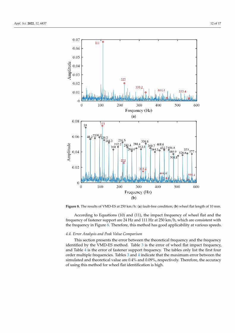
Figure 8. The results of VMD-ES at 250 km/h: (a) fault-free condition; (b) wheel flat length of 10 mm.

According to Equations (10) and (11), the impact frequency of wheel flat and the frequency of fastener support are 24 Hz and 111 Hz at 250 km/h, which are consistent with the frequency in Figure 8. Therefore, this method has good applicability at various speeds.

4.4. Error Analysis and Peak Value Comparison This section presents the error between the theoretical frequency and the frequency

identified by the VMD-ES method. Table 3 is the error of wheel flat impact frequency, and Table 4 is the error of fastener support frequency. The tables only list the first four order multiple frequencies. Table 3 and Table 4 indicate that the maximum error be-tween the simulated and theoretical value are 0.4% and 0.09%, respectively. Therefore, the accuracy of using this method for wheel flat identification is high.

Am

plitu

de

Figure 8. The results of VMD-ES at 250 km/h: (a) fault-free condition; (b) wheel flat length of 10 mm.

According to Equations (10) and (11), the impact frequency of wheel flat and thefrequency of fastener support are 24 Hz and 111 Hz at 250 km/h, which are consistent withthe frequency in Figure 8. Therefore, this method has good applicability at various speeds.

4.4. Error Analysis and Peak Value Comparison

This section presents the error between the theoretical frequency and the frequencyidentified by the VMD-ES method. Table 3 is the error of wheel flat impact frequency,and Table 4 is the error of fastener support frequency. The tables only list the first fourorder multiple frequencies. Tables 3 and 4 indicate that the maximum error between thesimulated and theoretical value are 0.4% and 0.09%, respectively. Therefore, the accuracyof using this method for wheel flat identification is high.

Appl. Sci. 2022, 12, 6837 13 of 17

Table 3. The error of the wheel flat impact frequency.

Speed Wheel Flat ImpactFrequency 1st Order 2nd Order 3rd Order 4th Order

250/(km/h−1)Theoretical value/Hz 24 48 72 96Simulated value/Hz 24 48.2 72 96.2

Error rate/% 0 0.4 0 0.2

350/(km/h−1)Theoretical value/Hz 33.6 67.2 100.8 134.4Simulated value/Hz 33.6 67.3 101 134.5

Error rate/% 0 0.1 0.2 0.07

Table 4. The error of the fastener support frequency.

Speed Fastener SupportFrequency 1st Order 2nd Order 3rd Order 4th Order

250/(km/h−1)Theoretical value/Hz 111 222 333 444Simulated value /Hz 111 222 333.2 444.4

Error rate/% 0 0 0.06 0.09

350/(km/h−1)Theoretical value/Hz 155.6 311.2 466.8 622.4Simulated value/Hz 155.6 311 466.8 622.7

Error rate/% 0 0.06 0 0.05

Figure 9 shows the relationship between the mean amplitude of the first four multiplefrequencies and the length of wheel flat at various speeds. It can be seen that the meanamplitude of the first four multiple frequencies in ES increases monotonically with thelength of flat, and the difference between the mean value at the same speed expands withthe increase of the wheel flat length. Hence, the mean value of the first four multiplefrequencies in ES can be used to quantitatively identify the wheel flat faults.

Appl. Sci. 2022, 12, x FOR PEER REVIEW 13 of 17

Table 3. The error of the wheel flat impact frequency.

Speed Wheel Flat Impact Frequency 1st Order 2nd Order 3rd Order 4th Order

250/(km/h−1) Theoretical value/Hz 24 48 72 96 Simulated value/Hz 24 48.2 72 96.2

Error rate/% 0 0.4 0 0.2

350/(km/h−1) Theoretical value/Hz 33.6 67.2 100.8 134.4 Simulated value/Hz 33.6 67.3 101 134.5

Error rate/% 0 0.1 0.2 0.07

Table 4. The error of the fastener support frequency.

Speed Fastener Support Frequency 1st Order 2nd Order 3rd Order 4th Order

250/(km/h−1) Theoretical value/Hz 111 222 333 444 Simulated value /Hz 111 222 333.2 444.4

Error rate/% 0 0 0.06 0.09

350/(km/h−1) Theoretical value/Hz 155.6 311.2 466.8 622.4 Simulated value/Hz 155.6 311 466.8 622.7

Error rate/% 0 0.06 0 0.05

Figure 9 shows the relationship between the mean amplitude of the first four mul-tiple frequencies and the length of wheel flat at various speeds. It can be seen that the mean amplitude of the first four multiple frequencies in ES increases monotonically with the length of flat, and the difference between the mean value at the same speed expands with the increase of the wheel flat length. Hence, the mean value of the first four multi-ple frequencies in ES can be used to quantitatively identify the wheel flat faults.

Figure 9. The relationship between the mean amplitude of the first four orders and the length of wheel flat.

5. Influence of the Wheel Eccentricity on Wheel Flat Identification The wheel may occur eccentricity during the running process, and its characteristic

frequency is 0 / (2 )f v R , which is consistent with the impact frequency of the wheel flat. Therefore, it is necessary to determine whether the wheel eccentricity may influence the accuracy of the wheel flat identification. Figure 10 is the result of the wheel eccen-tricity with 1 mm amplitude at 350 km/h by using the VMD-ES method. Figure 11 shows the results under the co-existence of the wheel eccentricity and wheel flat at the same

10 20 30 40 500.0

0.1

0.2

0.3

0.4

0.5

0.6

Am

plitu

de

Wheel flat length (mm)

250km/h 300km/h 350km/h

Figure 9. The relationship between the mean amplitude of the first four orders and the length ofwheel flat.

5. Influence of the Wheel Eccentricity on Wheel Flat Identification

The wheel may occur eccentricity during the running process, and its characteristicfrequency is f0 = v/(2πR), which is consistent with the impact frequency of the wheel flat.Therefore, it is necessary to determine whether the wheel eccentricity may influence theaccuracy of the wheel flat identification. Figure 10 is the result of the wheel eccentricitywith 1 mm amplitude at 350 km/h by using the VMD-ES method. Figure 11 shows the

Appl. Sci. 2022, 12, 6837 14 of 17

results under the co-existence of the wheel eccentricity and wheel flat at the same speed(the length of flat is 14 mm and the amplitude of wheel eccentricity is 1 mm). The resultsshow that only the dominant frequency (33.6 Hz) is presented in ES under the wheeleccentricity. Meanwhile, in the case of co-existence of the wheel eccentricity and flat, themultiple frequency generated by the wheel flat is reflected in ES. The mean amplitude ofthe first four multiple frequencies is almost the same with the value corresponding to thelength of a 14 mm flat in Figure 9. Therefore, the proposed method has good ability inwheel flat identification under the co-existence of the wheel eccentricity and flat.

Appl. Sci. 2022, 12, x FOR PEER REVIEW 14 of 17

speed (the length of flat is 14 mm and the amplitude of wheel eccentricity is 1 mm). The results show that only the dominant frequency (33.6 Hz) is presented in ES under the wheel eccentricity. Meanwhile, in the case of co-existence of the wheel eccentricity and flat, the multiple frequency generated by the wheel flat is reflected in ES. The mean am-plitude of the first four multiple frequencies is almost the same with the value corre-sponding to the length of a 14 mm flat in Figure 9. Therefore, the proposed method has good ability in wheel flat identification under the co-existence of the wheel eccentricity and flat.

Figure 10. The results of wheel eccentricity.

Figure 11. The results of the co-existence of wheel eccentricity and wheel flat.

6. Field Test Validation In this section, the axlebox acceleration was measured from the in-service vehicle

on a certain line at 75 km/h. The sampling frequency of the measured data is 4 kHz. Fig-ure 12 illustrates the placement of the axlebox acceleration sensor.

Am

plitu

de

Figure 10. The results of wheel eccentricity.

Appl. Sci. 2022, 12, x FOR PEER REVIEW 14 of 17

speed (the length of flat is 14 mm and the amplitude of wheel eccentricity is 1 mm). The results show that only the dominant frequency (33.6 Hz) is presented in ES under the wheel eccentricity. Meanwhile, in the case of co-existence of the wheel eccentricity and flat, the multiple frequency generated by the wheel flat is reflected in ES. The mean am-plitude of the first four multiple frequencies is almost the same with the value corre-sponding to the length of a 14 mm flat in Figure 9. Therefore, the proposed method has good ability in wheel flat identification under the co-existence of the wheel eccentricity and flat.

Figure 10. The results of wheel eccentricity.

Figure 11. The results of the co-existence of wheel eccentricity and wheel flat.

6. Field Test Validation In this section, the axlebox acceleration was measured from the in-service vehicle

on a certain line at 75 km/h. The sampling frequency of the measured data is 4 kHz. Fig-ure 12 illustrates the placement of the axlebox acceleration sensor.

Am

plitu

de

Figure 11. The results of the co-existence of wheel eccentricity and wheel flat.

6. Field Test Validation

In this section, the axlebox acceleration was measured from the in-service vehicle on acertain line at 75 km/h. The sampling frequency of the measured data is 4 kHz. Figure 12illustrates the placement of the axlebox acceleration sensor.

Appl. Sci. 2022, 12, 6837 15 of 17Appl. Sci. 2022, 12, x FOR PEER REVIEW 15 of 17

Figure 12. The placement of the axlebox acceleration sensor.

The measured data with the wheel flat is analyzed by the proposed VMD-ES meth-od; Figure 13a is the vertical axlebox acceleration signal with the length of 16 mm wheel flat and Figure 13b is the analysis of results using this method. The multiple frequency of the wheel flat impact are clearly represented in the results (the impact frequency is 7.2 Hz) which is consistent with the rule of the dynamics simulation. In the measured data, the mean value of the first four multiple frequencies under 16 mm wheel flat length is 0.075. Meanwhile, the value in Figure 9 is 0.078. The error rate between the simulation and measurement is 4%. The results verify the accuracy of the established vehicle dy-namic model. Therefore, the proposed VMD-ES method can detect the wheel flat fault from the strong interference signal.

(a) (b)

Figure 13. Field test: (a) the measured data; (b) The results of the measured data based on the VMD-ES method.

7. Conclusions This work proposes an on—board monitoring method based on the axlebox accel-

eration using the VMD—ES method. A three—dimensional vehicle—track coupled dy-namic model verified by field test was established to simulate the axlebox acceleration of a high—speed railway. The simulation and field test results show that the VMD–ES method accurately extracts the impact characteristics of the wheel flat and can quantita-tively identify the wheel flat faults at various speeds. Based on the results, the following conclusions can be drawn: (1) The axlebox acceleration includes strong interference signal excited by the rail and

wheel which influences the accurate identification of the wheel flat. The results

Figure 12. The placement of the axlebox acceleration sensor.

The measured data with the wheel flat is analyzed by the proposed VMD-ES method;Figure 13a is the vertical axlebox acceleration signal with the length of 16 mm wheel flatand Figure 13b is the analysis of results using this method. The multiple frequency of thewheel flat impact are clearly represented in the results (the impact frequency is 7.2 Hz)which is consistent with the rule of the dynamics simulation. In the measured data, themean value of the first four multiple frequencies under 16 mm wheel flat length is 0.075.Meanwhile, the value in Figure 9 is 0.078. The error rate between the simulation andmeasurement is 4%. The results verify the accuracy of the established vehicle dynamicmodel. Therefore, the proposed VMD-ES method can detect the wheel flat fault from thestrong interference signal.

Appl. Sci. 2022, 12, x FOR PEER REVIEW 15 of 17

Figure 12. The placement of the axlebox acceleration sensor.

The measured data with the wheel flat is analyzed by the proposed VMD-ES meth-od; Figure 13a is the vertical axlebox acceleration signal with the length of 16 mm wheel flat and Figure 13b is the analysis of results using this method. The multiple frequency of the wheel flat impact are clearly represented in the results (the impact frequency is 7.2 Hz) which is consistent with the rule of the dynamics simulation. In the measured data, the mean value of the first four multiple frequencies under 16 mm wheel flat length is 0.075. Meanwhile, the value in Figure 9 is 0.078. The error rate between the simulation and measurement is 4%. The results verify the accuracy of the established vehicle dy-namic model. Therefore, the proposed VMD-ES method can detect the wheel flat fault from the strong interference signal.

(a) (b)

Figure 13. Field test: (a) the measured data; (b) The results of the measured data based on the VMD-ES method.

7. Conclusions This work proposes an on—board monitoring method based on the axlebox accel-

eration using the VMD—ES method. A three—dimensional vehicle—track coupled dy-namic model verified by field test was established to simulate the axlebox acceleration of a high—speed railway. The simulation and field test results show that the VMD–ES method accurately extracts the impact characteristics of the wheel flat and can quantita-tively identify the wheel flat faults at various speeds. Based on the results, the following conclusions can be drawn: (1) The axlebox acceleration includes strong interference signal excited by the rail and

wheel which influences the accurate identification of the wheel flat. The results

Figure 13. Field test: (a) the measured data; (b) The results of the measured data based on theVMD-ES method.

7. Conclusions

This work proposes an on—board monitoring method based on the axlebox accelera-tion using the VMD—ES method. A three—dimensional vehicle—track coupled dynamicmodel verified by field test was established to simulate the axlebox acceleration of ahigh—speed railway. The simulation and field test results show that the VMD–ES methodaccurately extracts the impact characteristics of the wheel flat and can quantitatively iden-tify the wheel flat faults at various speeds. Based on the results, the following conclusionscan be drawn:

Appl. Sci. 2022, 12, 6837 16 of 17

(1) The axlebox acceleration includes strong interference signal excited by the rail andwheel which influences the accurate identification of the wheel flat. The results showthat the proposed VMD–ES method accurately extracts the characteristic frequency ofthe wheel flat from complex frequency components. Meanwhile, the mean amplitudeof the first four multiple frequency increases monotonically with the length of flatin ES. Therefore, the VMD–ES method can be applied to quantitatively identify thewheel flat faults at various speeds.

(2) In the case of the wheel eccentricity, only the dominant frequency (33.6 Hz) is pre-sented in the results of ES. At the co-existence of the wheel eccentricity and flat, theVMD–ES method can accurately extract the multiple frequency of the wheel flat. Themethod has good adaptability in wheel flat identification; wheel eccentricity has noinfluence on the detection.

(3) The field test is carried out to verify the accuracy of the method. The results of thefield test are consistent with the simulation results, which reflect the correctness of theestablished vehicle-track coupled dynamics model, and the feasibility of the wheelflat identification by using this method.

In this paper, the wheel flat detection is investigated in detail by using the VMD-EDmethod. The results show that the method can quantitatively identify the wheel flat faultsat various speeds. Machine learning methods will be combined with advanced signalprocessing techniques to identify the wheel flat in our future work.

Author Contributions: X.L.: Conceptualization, Methodology, Writing original draft, Software. Z.H.:Supervision, Resources, Writing—review and editing. Y.W., L.Y. and H.W.: Validation. L.C.: Field testinstruction. All authors have read and agreed to the published version of the manuscript.

Funding: This work was supported by the National Natural Science Foundation of China, grantnumbers 52162047, 52062028, the Natural Science Foundation of Gansu Province, grant number20JR5RA393, and the opening foundation of the State Key Laboratory of Traction Power in SouthwestJiaotong University, grant number TPL1902.

Institutional Review Board Statement: Not applicable.

Informed Consent Statement: Not applicable.

Data Availability Statement: Not applicable.

Conflicts of Interest: The authors declare no conflict of interest.

References1. Wang, Z.; Allen, P.; Mei, G.; Yin, Z.; Cheng, Y.; Zhang, W. Dynamic characteristics of a high-speed train gearbox in the vehicle–track

coupled system excited by wheel defects. Proc. Inst. Mech. Eng. Part F J. Rail Rapid Transit 2020, 234, 1210–1226. [CrossRef]2. Wang, Z.; Mo, J.; Gebreyohanes, M.Y.; Wang, K.; Wang, J.; Zhou, Z. Dynamic response analysis of the brake disc of a high-speed

train with wheel flats. Proc. Inst. Mech. Eng. Part F J. Rail Rapid Transit 2022, 236, 593–605. [CrossRef]3. Masoudi Nejad, R.; Noroozian Rizi, P.; Zoei, M.S.; Aliakbari, K.; Ghasemi, H. Failure Analysis of a Working Roll Under the

Influence of the Stress Field Due to Hot Rolling Process. J. Fail. Anal. Prev. 2021, 21, 870–879. [CrossRef]4. Bian, J.; Gu, Y.; Murray, M.H. A dynamic wheel-rail Impact analysis of rail rail track under Wheel flat by finite element analysis.

Veh. Syst. Dyn. 2013, 51, 784–797. [CrossRef]5. Bernal, E.; Spiryagin, M.; Cole, C. Onboard condition monitoring sensors, systems and techniques for freight railway vehicles: A

Review. IEEE Sens. J. 2019, 19, 4–24. [CrossRef]6. Mosleh, A.; Montenegro, P.A.; Costa, P.A.; Calçada, R. Railway vehicle wheel flat detection with multiple records using spectral

kurtosis analysis. Appl. Sci. 2021, 11, 4002. [CrossRef]7. Alemi, A.; Corman, F.; Pang, Y.; Lodewijks, G. Reconstruction of an informative railway wheel defect signal from wheel-rail

contact signals measured by multiple wayside sensors. Proc. Inst. Mech. Eng. Part F J. Rail Rapid Transit 2019, 233, 49–62.[CrossRef]

8. Cao, W.; Zhang, S.; Bertola, N.J.; Smith, I.F.C.; Koh, C.G. Time series data interpretation for ‘wheel-flat’ identification includinguncertainties. Struct. Health Monit. 2019. [CrossRef]

9. Salzburger, H.J.; Schuppmann, M.; Li, W.; Gao, X. In-motion ultrasonic testing of the tread of high-speed railway wheels usingthe inspection system AUROPA III. Insight—Non-Destructive Test. Cond. Monit. 2009, 51, 370–372.

Appl. Sci. 2022, 12, 6837 17 of 17

10. Brizuela, J.; Ibañez, A.; Nevado, P.; Fritsch, C. Railway wheels flat detector using Doppler effect. Phys. Procedia 2010, 3, 811–817.[CrossRef]

11. Brizuela, J.; Fritsch, C.; Ibáñez, A. Railway wheel-flat detection and measurement by ultrasound. Transp. Res. Part C Emerg. Technol.2011, 19, 975–984. [CrossRef]

12. Lai, C.C.; Kam, J.C.P.; Leung, D.C.C.; Lee, T.K.Y.; Tam, A.Y.M.; Ho, S.L.; Tam, H.Y.; Liu, M.S.Y. Development of a fiber-opticsensing system for train vibration and train weight measurements in Hong Kong. J. Sens. 2012, 2012, 1–7. [CrossRef]

13. Tam, H.Y.; Liu, S.Y.; Guan, B.O.; Chung, W.H.; Chan, T.H.T.; Cheng, L.K. Fiber Bragg Grating sensors for structural and railwayapplications. In Proceedings of the SPIE-The International Society for Optical Engineering, Beijing, China, 8 November 2004;pp. 85–97.

14. Wei, C.; Lai, C.; Liu, S.; Chung, W.H.; Ho, T.K.; Tam, H.; Ho, S.L.; McCusker, A.; Kam, J.; Lee, K.Y. A Fiber Bragg Grating sensorsystem for train axle counting. IEEE Sens. J. 2010, 10, 1905–1912.

15. Filograno, M.L.; Rodriguez-Barrios, A.; González-Herraez, M.; Corredera, P.; Martín-López, S.; Rodríguez-Plaza, M.;Andrés-Alguacil, A. Real-time monitoring of railway traffic using Fiber Bragg Grating sensors. IEEE Sens. J. 2012, 12, 85–92.[CrossRef]

16. Alemi, A.; Corman, F.; Lodewijks, G. Condition monitoring approaches for the detection of railway wheel defects.Proc. Inst. Mech. Eng. Part F J. Rail Rapid Transit 2017, 231, 961–981. [CrossRef]

17. Liang, B.; Iwnicki, S.; Ball, A.; Young, A.E. Adaptive noise cancelling and time–frequency techniques for rail surface defectdetection. Mech. Syst. Signal Process. 2014, 54–55, 41–51. [CrossRef]

18. Bosso, N.; Gugliotta, A.; Zamperi, N. Wheel flat detection algorithm for onboard diagnostic. Measurement 2018, 123, 193–202.[CrossRef]

19. Shim, J.; Kim, G.; Cho, B.; Koo, J. Application of vibration signal processing methods to detect and diagnose wheel flats in railwayvehicles. Appl. Sci. 2021, 11, 2151. [CrossRef]

20. Shi, D.; Ye, Y.; Gillwal, M.; Hecht, M. Designing a lightweight 1D convolutional neural network with Bayesian optimization forwheel flat detection using carbody accelerations. Int. J. Rail Transp. 2020, 9, 311–341. [CrossRef]

21. Bernal, E.; Spiryagin, M.; Cole, C. Wheel flat analogue fault detector verification study under dynamic testing conditions using ascaled bogie test rig. Int. J. Rail Transp. 2021, 10, 177–194. [CrossRef]

22. Huang, N.E.; Shen, Z.; Long, S.R.; Wu, M.C.; Shih, H.H.; Zheng, Q.; Yen, N.; Tung, C.C.; Liu, H.H. The empirical mode decomposi-tion and the hilbert spectrum for nonlinear and non-stationary time series analysis. Proc. R. Soc. Lond. Ser. A Math. Phys. Eng. Sci.1998, 454, 903–995. [CrossRef]

23. Li, Y.; Zuo, M.J.; Lin, J.; Liu, J. Fault detection method for railway wheel flat using an adaptive multiscale morphological filter.Mech. Syst. Signal Process. 2017, 84, 642–658. [CrossRef]

24. Li, Y.; Liu, J.; Wang, Y. Railway wheel flat detection based on improved empirical mode decomposition. Shock Vib. 2016,2016, 4879283. [CrossRef]

25. Chen, S.; Wang, K.; Chang, C.; Xie, B.; Zhai, W. A two-level adaptive chirp mode decomposition method for the railway wheelflat detection under variable-speed conditions. J. Sound Vib. 2021, 498, 115963. [CrossRef]

26. Dragomiretskiy, K.; Zosso, D. Variational mode decomposition. IEEE Trans. Signal Process. 2014, 62, 531–544. [CrossRef]27. Zhu, S.; Xia, H.; Peng, B.; Zio, E.; Wang, Z.; Jiang, Y. Feature extraction for early fault detection in rotating machinery of nuclear

power plants based on adaptive VMD and Teager energy operator. Ann. Nucl. Energy 2021, 160, 108392. [CrossRef]28. Jin, Z.; He, D.; Wei, Z. Intelligent fault diagnosis of train axle box bearing based on parameter optimization VMD and improved

DBN. Eng. Appl. Artif. Intel. 2022, 110, 104713. [CrossRef]29. Li, H.; Liu, T.; Wu, X.; Chen, Q. An optimized VMD method and its applications in bearing fault diagnosis. Measurement 2020,

166, 108185. [CrossRef]30. Bernal, E.; Spiryagin, M.; Cole, C. Wheel flat detectability for Y25 railway freight wagon using vehicle component acceleration

signals. Veh. Syst. Dyn. 2020, 58, 1893–1913. [CrossRef]31. Zhai, W. Vehicle-Track Coupled Dynamics Theory and Applications; Springer: Singapore, 2020.32. Wu, T.; Thompson, D. A hybrid model for the noise generation due to railway wheel flats. J. Sound Vib. 2002, 251, 115–139.

[CrossRef]33. Yang, J.; Zhou, C.; Li, X. Research on Fault Feature Extraction Method Based on Parameter Optimized Variational Mode

Decomposition and Robust Independent Component Analysis. Coatings 2022, 12, 419. [CrossRef]