148 T h e V a lu a tio n o f M o rtg a g e B a ck ed S ecu rities w ith S to ch a stic:::

V o lu m en 1 , N ¶u m ero 2 (2 0 0 7 ), p p . 1 4 8 -1 6 8 w w w .csf.itesm .m x / eg a d e/ p u b lica cio n es

R ecib id o 1 5 d e m a rzo 2 0 0 7 , A cep ta d o 6 d e ju n io 2 0 0 7

T h e V alu ation of M ortgage B acked S ecu rities

w ith S to ch astic P rob ab ilities ofD efau lt an d P rep ay m en t

F ra n c isc o V e n e g a s-M a rt¶³n e z ¤

J . V ic to r R e y n o so -V e n d re ll¤ ¤

A b str a c t

The aim of this paper is to provide a new approach to pro ject the MortgageBacked Securities (MBS) cash °ows in emerging markets where collateralinformation is limited, wrong or scarce. Under this framework, we used theCox Process to model stochastic probabilities of prepayment and default. Themodel deals with general intensity dynamics and is applied to the starting MBSMexican market.

R e su m e n

En este art¶³culo se propone una nueva metodolog¶³a para la proyecci¶on de los°uj os de bonos respaldados por hipotecas (BORHIS) en mercados emergentesdonde la informaci¶on del colateral es limitada, incorrecta o incompleta. Baj oesta metodolog¶³a se utiliza el proceso de Cox para modelar las probabilidadesestoc¶asticas de prepago e incumplimiento. El modelo utiliza una din¶amicageneral en la intensidad, la cual se aplica en el naciente mercado de BORHIS.

C la si caci¶o n J E L : G 12 , G 13 a n d G 1 4.

P a lab ras clav e: M ortg a ge valu a tion , M B S p rep ay m en t, M B S d efa u lt, M B S cu rtailm en t, C ox

P ro cess.

1 . In tr o d u c tio n

The Mortgage Backed Securities (MBS) market is j ust growing in Mexico. Theoldest MBS was sold to the investors in December 2003. In the following years2004 and 2005, 250 million USD were put on the market each year, and in 2006this amount increased 330%. Currently, there are approximately 2 billion USD(in April 2007) in assets backed with mortgage loans1 . The government agency

¤ In v estig a d o r E S E -IP N .¤ ¤ S u b d irecto r M B S / A B S R isk M a n a g em en t H S B C M ¶ex ico , m a il:

jo se.V .R E Y N O S O @ h sb c.co m .m x1 S o u rce: S H F , A p ril 2 0 0 7 . (h ttp :/ / w w w .sh f.g o b .m x / ¯ les/ p d f/ B O R H IS 0 4 0 7 1 .p d f)

F ra n cisco V en eg a s-M a rt¶³n ez y J . V icto r R ey n o so -V en d rell 149

that promotes the MBS market is \Sociedad Hipotecaria Federal" (SHF) . Thisagency not only provides the funding for mortgage banks, but also attempts tocreate the MBS market (primary and secondary) so as to change the fundingfrom government to investor with the mortgage backed securities.

As known, the two risky events in the mortgage world are the prepaymentand default events. The ¯rst one is related to the possibility that the borrowerprepays the loan before maturity without penalty, so the investor has to reinvesthis money in a new mortgage loan at the current rate, losing the di®erencebetween the old loan rate and the new one if the current coupon is lower, whichis the most frequent case because the borrower prepays the old mortgage tore¯nance his debt with a lower rate. Of course, there are many other causesto prepay the loan making a di±cult task to forecast the mortgager cash °ows.The second risky event is the possibility that the borrower does not pay hisdebt and the house has to be sold at stressed prices.

The literature related to the valuation of this kind of assets is veryextensive; see for instance: Fabozzi (2006) , Davidson (2003) and Austin (2005) ,j ust to mention a few ones. However, most of this literature deals with the USAmarket case where many statistical or econometrics approaches have been usedin modeling probabilities of prepayment and default. However, when modelingsuch probabilities it is important to mention that there are two main di®erencesbetween the USA case and the emerging markets case. The ¯rst one is that mostof the MBS credit risk is practically nonexistent (government agencies maintainthis risk, 65% of the market) 2 , and the second one, and most important, is themarket liquidity.

In contrast with the USA case, the emerging markets have very poor orscarce information, so our approach has to be di®erent. The market participantsnot only have to consider all international experience and knowledge to valueand deal with this new ¯nancial instrument dependent on local environment,but also have to be creative to deal with missing information.

This paper is an e®ort to provide a new approach for the emerging marketscase to price and deal with risk management of the mortgage related assets. Themodel recognizes the random behavior of the cash °ows by using stochasticprobabilities of default and prepayment. After the cash °ows are modeled, theMBS (subordinated or senior tra n ch e) is the present value of the aggregated anddistributed °ows with the structure waterfall (the money distribution rules) .

The paper is organized as follow; the next section deals with the mortgageloans basic e®ects. Section 3 provides the underlying theory to construct thestochastic probabilities of prepayment and default. Section 4 assigns stochas-tic probabilities of prepayment and default. Section 5 is a simple but realisticimplementation with the collateral (mortgage pool) information from theMexican market (BRHCGCB-03U) . Section 6 presents conclusions, acknowl-edges limitations, and makes suggestions for further research.

2 S o u rce: IM F , G lo b a l F in a n cia l S ta b ility R ep o rt, M a rk et D ev elo p m en t a n d Issu es, C h a p -

ter I, A p ril 2 0 0 7 , (h ttp :/ / w w w .im f.o rg / ex tern a l/ p u b s/ ft/ g fsr/ 2 0 0 7 / 0 1 / in d ex .h tm ).

150 T h e V a lu a tio n o f M o rtg a g e B a ck ed S ecu rities w ith S to ch a stic:::

2 . L o a n C a sh ° o w s

The ¯rst step for the valuation of any security backed with mortgage loansis to know the collateral cash °ow dynamics, this °ow is generated from themortgage pool. We will be modeling the cash °ow of an individual loan andthen aggregate the loans to complete the collateral cash °ow.

The loans that we will be considering in the modeling are mortgage withequal payments, ¯xed rate loans, and mortgage with °oating payments,adj ustable rate mortgages, and every month or payment day some part of thepayment goes to principal and the other part to interest, also the borrower canprepay the total or some additional part of the outstanding balance with nocost, which is the most common case in Mexican mortgage market.

Every payment day we have a scheduled payment of principal (PO) andinterest (IO) , but the borrower has at least three more possibilities; eitherpaying more principal than the scheduled (curtailment) , prepaying the totalloan balance (prepayment) or not paying (delinquency) , these e®ects makes theassets collateralized with mortgage very speculative.

We start by introducing some notation before we proceed to work onformulas, the payment dates are denoted by t = (t0 ;t1 ;:::;tn ) with t0 the initialdate and tn the last scheduled payment date. The original balance is denotedby B (t0 ) , and the scheduled payment of principal and interest is P M T (t) , thenthe ¯rst expected °ow is:

F lo w (t1 ) = (P M T (t1 )| {z }P ay m en t

+ ¿ (t1 ) )B (t1 ) ¸ C (t1 ) (1 ¡ ¸ P (t1 ) )| {z }

C u rta ilm en t

(I O + P O )

+ B (t1 )¸ P (t1 ) (1 ¡ ¸ C (t1 ) )| {z }

P rep ay m en t

(1 ¡ ¸ D el(t1 ) )| {z }

D elin q u en cy

(1)

where:

¸ C (t1 ) : Probability that the borrower prepays at time t1 moreprincipal that the scheduled but not the total balance, this situation iscalled curtailment.

¸ P (t1 ) : Conditional probability that the borrower prepays the total loanbalance at time t1 given that the borrower did not prepay before.

¸ D el(t1 ) : Probability that the borrower does not pay at time t1 , thissituation is called delinquency.

¿ (t1 ) Percentage of the loan balance at time t1 which is prepaid.

Equation (1) re°ects the di®erent possibilities of the °ow at the ¯rstpayment day, t1 , which are the payment amount if there is no delinquency, thecurtailment and the total prepayment. At time t2 , it is more complicated be-cause the balance, after the ¯rst payment date, has many di®erent possibilitiesdepending on the amount of curtailment or delinquency and the Flow(t2 ) isdependent on the ¯rst payment, then the next expected cash °ow is:

F ra n cisco V en eg a s-M a rt¶³n ez y J . V icto r R ey n o so -V en d rell 151

F lo w (t2 ) = (P M T (t2 ) + ¿ (t2 ) (B (t2 jC (t1 ) )¸ C (t1 ) + B (t2 )S C (t1 ) ) ¸ C (t2 )

S P (t2 ) ) S D el(t2 ) +¡B (t2 jC (t1 ) )¸ C (t1 ) + B (t2 )S C (t1 )

¢¸ P (t2 ) S P (t1 )

S C (t1 )S D el(t2 ) +¡P M T (t1 ) + P M T (t2 ) + ¿ (t2 )B (t2 )¸ C (t2 )

(1 ¡ ¸ P (t2 ) ) +¡B (t2 )¸ P (t2 ) (1 ¡ ¸ C (t2 ) )

¢¢¸ D el(t1 ) (1 ¡ ¸ D el(t2 ) )

(2)

where:B (t2 jC (t1 ) ) : Balance at time t2 , given that the loan had a curtailment attime t1 .

B (t2 ) : Scheduled balance.

S C (tn ) =

nY

i= 1

(1 ¡ ¸ C (ti) ) ;

S P (tn ) =

nY

i= 1

(1 ¡ ¸ P (ti) ) ;

S D el(tn ) =

nY

i= 1

(1 ¡ ¸ D el(ti) ) :

The last equation looks complicate because the di®erent paths of the balancebuild a non-recombining lattice; the curtailment at time t1 and no curtailmentat time t2 ¯nishing with di®erent balance than no curtailment at time t1 andcurtailment at time t2 , making the implementation computational di±cult andintensive.

To simplify the analysis, we will consider that the probability of curtail-ment is one, this means that every payment day the borrower prepays an extraamount of principal. This assumption is not dangerous because we are goingto aggregate the pool of loans and is very common that a few loans does somecurtailment, then we replace equation (1) with:

F lo w (t1 ) = (P M T (t1 ) + ¿ (t1 ) (B (t0 ) ¡ (P M T (t1 ) ¡ I O (t1 ) ) ) + B (t1 )

¸ P (t1 ) ) (1 ¡ ¸ D el(t1 ) )(3)

where: I O (t1 ) = B (t0 ) r M (t0 ) , interest in the ¯rst payment day; r M (t0 ) ,e®ective mortgage rate in the time t0 y B (t1 ) = B (t0 ) ¡ (P M T (t0 ) ¡ I O (t1 ) ) ¡¿ (t1 ) (B (t0 ) ¡ (P M T (t0 ) ¡ I O (t1 ) ) ) , principal outstanding after the curtailment.

Now the prepayment is over the remaining balance after the curtailment.The °ow at time t2 is:

F lo w (t2 ) = (P M T (t2 ) + ¿ (t2 ) (B (t1 ) ¡ (P M T (t2 ) ¡ I O (t2 ) ) ) + B (t2 ) ¸ P (t2 ) )

S D el(t2 )S P (t1 ) + (P M T (t1 ) + P M T (t2 ) + ¿ (t2 ) (B (t1 )¡(P M T (t2 ) ¡ I O (t2 ) ) ) + B (t2 )¸ P (t2 ) ) ¸ D el(t1 ) (1 ¡ ¸ D el(t2 ) )

(4)

152 T h e V a lu a tio n o f M o rtg a g e B a ck ed S ecu rities w ith S to ch a stic:::

Even thought the above formula is simpler than the complete process, we willmake an additional assumption when changing from delinquency to default;the di®erence between these two e®ects is that once the borrower is in defaulthe will never pay again, and delinquency assume that the borrower would becurrent again (pay again) , the usual time to change from delinquency to defaultis three consecutive months of delinquency. Now, we have that the °ow at timetn is:

F lo w (tn ) = (P M T (tn ) + ¿ (tn ) (B (tn ¡ 1 ) ¡ (P M T (tn ) ¡ I O (tn ) ) ) + B (tn )

¸ P (tn ) ) S D (tn ) S P (tn ¡ 1 )(5)

whereS D (tn ) =

Q ni= 1 (1 ¡ ¸ D (ti) ) : Surviving probability or not be in default

before the time tn .

¸ D (tn ) ) : Conditional probability that the borrower default in the time tn ,given that the borrower did not default before.

B (tn ) = B (tn ¡ 1 ) ¡ (P M T (tn ) ¡ I O (tn ) ) : Outstanding balance after thescheduled principal payment.

I O (tn ) = B (tn ¡ 1 ) r M (tn ) : Interest paid in the time tn .

The next step is the estimation of the two conditional probabilities ofdefault and prepayment, and the curtailment rate. Once we have these proba-bilities, we may calculate the future cash °ows and aggregate the °ows of everyloan to have the total pool °ows, the basic element in the valuation and riskmanagement of MBS. In the next section, we will explore the di®erent methodsto estimate the default, prepayment and the curtailment rate.

3 . T h e o r e tic a l F r a m e w o r k

This section establishes the statistics underlying the prepayment and defaultmodeling. Both events can be expressed as the ¯rst j ump of a point process,which is the event we want to forecast by using the characteristics of the loan,borrower and the economic environment in which the mortgagor and the marketinteract.

Every month, we will expect some default and prepayment in the pool ofloans, no loan can be prepaid twice and we will assume that no loan can bedefaulted twice, although in reality some of them can be in default and thencured.

In the pool or sample we observe n loans (i = 1;:::;n ) with continuoussurvival times T 1 , T 2 ,::: ,T n , nevertheless, we will work thinking of j ust oneloan and at the end we will aggregate the °ows. The borrower or loan survivalfunction in the pool is S with hazard rate ® , the hazard rate is the probabilityof failure in the next instant t + d t conditional of being alive in t, we expressthis as:

® =f

1 ¡ F(6)

where F is the distribution function at time T i and f is the density, thecomplement of the distribution function is the survival, S = 1 ¡ F .

F ra n cisco V en eg a s-M a rt¶³n ez y J . V icto r R ey n o so -V en d rell 153

The hazard rate completely determines the distribution trough the relation:

S (t) = P (T i > t) =

tY

0

[1 ¡ ® (s ) d s ] ¼ exp

µ¡Z t

0

® (s ) d s

¶; (7)

where the product function means a product-integral; the product over a 1= npartition of the interval [0;t] , 0 < t0 < t1 < ¢¢¢ < tn = t and taking thedi®erences to the limit of zero:

tY

0

[1 ¡ ® (s )d s ] = limm a x jti¡ ti¡ 1 j! 0

Y[1 ¡ (® (ti) ¡ ® (ti¡ 1 ) ) ] : (8)

The interpretation of the hazard rate ® is the probability of failure in the nextinstant given that the failure is grater that t:

P (T i 2 [t;t + d t)jT i ¸ t) = ® (t)d t (9)

The default/prepayment is the ¯rst j ump of the counting process:

N (t) = 1 f T i· tg (10)

and the intensity of the j ump process is:

¸ (t) = Y (t) ® (t) ; (11)

where Y i(t) = 1 f ¿i¸ tg , is a right continuous predictable process.

Now we are going to write the di®erence from time t to t+ d t of the countingprocess as d (N (t) ) , meaning N ((t + d t)¡ ) ¡ N (t¡ ) , and the expected value isthe intensity:

E[d N (t)j= t¡ ] = ¸ (t) d t: (12)

The cumulative intensity is called the compensator:

¤(t) =

Z t

0

¸ (s ) d s ; t ¸ 0: (13)

The compensated counting process or counting process martingale is thedi®erence between the counting process and the cumulative intensity, that is

M (t) = N (t) ¡ ¤(t) ; (14)

or, equivalently:

d N (t) = d ¤(t) + d M (t) = ¸ (t) d t + d M (t): (15)

Consider now a probability space (−;= ;P ) equipped the ¯ltration F = (= ) t2 R, a increasing right-continuous family of sub ¾ -algebras of = . Consider also the

154 T h e V a lu a tio n o f M o rtg a g e B a ck ed S ecu rities w ith S to ch a stic:::

conditional expectation of the increment of the process M , given the informationavailable we have:

E[d M (t)j= t¡ ] = E[d N (t) ¡ d ¤(t)j= t¡ ]

= E[d N (t) ¡ ¸ (t) d tj= t¡ ]

= E[d N (t)j= t¡ ] ¡ ¸ (t)d t

= 0

(16)

In modeling the intensity, the error has to be j ust noise and the model is ourbest guess about the failure of the loans in the future. Now, we will ¯nd thevariance of the noise in the model, which is known in the martingale theory asthe predictable variation and denoted by hM i:

Var[d M (t)j= t¡ ] = E[d M (t) 2 ]

= E[d N (t) 2 ] ¡ d ¤(t)

= d ¤(t) (1 ¡ d ¤(t) ):

(17)

Thus, the probability of default and prepayment can be estimated with theinformation of the pool, in the developed countries such as USA where theinformation is available, a lot of statistical tools can be used to get these proba-bilities, like logistic regression, survival theory or Generalized Additive Modelsof Hastie and Tibshirani (1986) .

In the emerging markets other assumptions has to be made because theinformation is incomplete and with low quality, then we will incorporate thisstylized fact, and we will recognize that the probability of default/prepaymentis unknown or stochastic, to do that we will use the Cox Process, which in-corporates an stochastic intensity. We take the de¯nition as in SchÄonbucher(2003) : Cox process: A point process N (t) with intensity ¸ (t) is a Cox pro-cess if, conditional on the background information & , N (t) is an inhomogeneousPoisson process with intensity ¸ (t) .

The background information is a ¯ltration (&) t¸ 0 with all the future andthe past information related to the intensity (the economical information, theborrower characteristics, etc. ) except the counting process or the j umps whichare in = t, and then the complete ¯ltration is:

¡= T o ta lt¸ 0

¢t¸ 0

= (= t¸ 0 ) t¸ 0 _ (&t¸ 0 ) t¸ 0 : (18)

The inhomogeneous Poisson process is similar to the Poisson process, but withan intensity ¸ (t) , a non-negative function of time. We will use again SchÄon-bucher (2003) de¯nition: Inhomogeneous Poisson process: An inhomogeneousPoisson process with intensity function ¸ (t) > 0 is a non-decreasing, integer-valued process with initial value N (0) = 0 whose increments are independentand satisfy,

P [N (T ) ¡ N (t) = n ] =1

n !

à Z T

t

¸ (s ) d s

!nexp

Ã

¡Z T

t

¸ (s )d s

!

: (19)

F ra n cisco V en eg a s-M a rt¶³n ez y J . V icto r R ey n o so -V en d rell 155

In the next section we will show how to incorporate this technology to themortgage loans assuming some stochastic dynamic to the intensity of prepay-ment and default. Incorporating this technology to the mortgage loans °ows wecan do a better pricing and risk management because we are recognizing thatwe really do not know the conditional probability of default/prepayment andwe will need to wait many years (at least 7 years) to know the real borrowerbehavior over the loan live.

4 . M o r tg a g e F lo w s w ith S to c h a stic In te n sity o f D e fa u lt a n d

P r e p a y m e n t

We will assume a Gaussian stochastic dynamic for the prepayment and defaultintensities with negative correlation between them. It is natural to assume thatthe borrower with problems to pay his debt hardly will prepay the whole bal-ance, and then if the probability of default is high the probability of prepaymentis low.

We can also incorporate the relation between the prepayment and the mort-gage rates, when the borrower has a higher coupon than the current marketcoupon he is tempted to go with other mortgage bank and get a new loan withlower rate, with this money he will prepaid the current mortgage loan, thisphenomena is called re¯nance. In Mexico this e®ect is not very clear becausethe mortgage rates moves very slow (low volatility) mainly because the marketis under development and the credit spread is high enough to absorb all thedaily volatility of the funding rate, nevertheless with the securitization of themortgage loans via MBS and the competence the market will grow faster andthe pricing of the credit spread will be better.

Other variables like the Loan to Value (LTV) 3 , Debt to Income (DTI) 4 orany other variable related to the borrower or the economy can be incorporatedin the mean of the intensity of prepayment or default, so the model has a good°exibility to ¯t the complexity involved in the borrower behavior.

We will assume the following stochastic dynamic for the intensities:

d ¸ P (t) = ¹ ¸ P (t;¯ ;r M (t) )d t + ¾ ¸ P d W (t); (20)

d ¸ D (t) = ¹ ¸ D (t; ¹) d t + ¾ ¸ D d ¹W (t) ; (21)

d W d ¹W = ½ d t; (22)

where¯ : Vector with all the relevant variables or covariates related to the pre-payment, like LTV, loan size, seasonality, etc.r M (t) : Stochastic market mortgage rate.¹: Vector with all the relevant variables or covariates related to the default,like LTV, DTI, etc.

W : Wiener process.

3 L o a n to V a lu e is th e lo a n p rin cip a l o u tsta n d in g d iv id ed b y th e va lu e o f th e co lla tera l o r

th e h o u se p rice.4 D eb t to In co m e is th e to ta l d eb t o f th e b o rrow er d iv id ed b y h is in co m e.

156 T h e V a lu a tio n o f M o rtg a g e B a ck ed S ecu rities w ith S to ch a stic:::

The mean of the prepayment intensity process, ¹ ¸ P (t;¯ ;r M (t) ) , has allthe important information of the market, loan and borrower characteristics. Infact, if we assume ¾ ¸ P = 0, we get one of the standard econometric model usedin the USA case.

With this model, the intensities are stochastic and the formula (5) leadsto the following expected value:

E[F lo w (tn )j= t0 ] = E [(P M T (tn ) + ¿ (tn ) (B (tn ¡ 1 ) ¡ (P M T (tn ) ¡ I O (tn ) ) )

+B (tn ) ¸ P (tn ) )S D (tn ) S P (tn ¡ 1 )j= t0¤

(23)In order to manipulate the above formula, we will assume continuous time,hence

E[F lo w (t)j= 0 ] = E [(P M T (t) + ¿ (t) (B (t¡ ) ¡ (P M T (t) ¡ I O (t) ) )

+B (t)¸ P (t) )S D (t)S P (t¡ )j= 0¤ (24)

where

t¡ = lim¢ ! 0 (t ¡ ¢);

S D (t) = exp

µ¡Z t

0

µ¸ D (0) +

Z u

0

¹ ¸ D (s ; ¹) d s + ¾ ¸ D (W (u ) ¡ W (0) )

¶d u

¶;

t¡ = lim¢ ! 0

(t ¡ ¢) ;

S P (t) = exp

µ¡Z t

0

µ¸ P (0) +

Z u

0

¹ ¸ P (s ; ¹;r M (s ) )d s + ¾ ¸ P (W (u ) ¡ W (0) )

¶

d u

¶;

The mean of these intensities processes can be stochastic because they maybe dependent to economical variables like the interest rate or the employment,but with the theorem of iterated expectation and the background information,which contains all the economy future information and the borrower character-istics, we can simplify the problem by using the fact:

E[E[F lo w (t)j&t ] ] : (25)

Under the conditional expectation given the background ¯ltration, the meanof the intensity is deterministic and we can use all the literature related to theinterest rates model (see Venegas 2006) to solve the expectation. The generalmethodology is as follows; ¯rst solve the expectation, E[F lo w (t)j&t ] , assumingthat all the economical variables are deterministic, after that the only stochasticvariables are those related to the economy, so the second expectation can besolve with Monte Carlo simulation.

To show a simpli¯ed version of the model, we will assume constant means ofdefault and prepayment (¹ ¸ D ;¹ ¸ P ) , subsequently we solve the expected value,¯nishing with a closed formula easy to implement.

F ra n cisco V en eg a s-M a rt¶³n ez y J . V icto r R ey n o so -V en d rell 157

The formula to calculate the cash °ows in the time 0 · s < t with constantmean of prepayment and default, and correlation ½ is:

E[F lo w (t)j= s ] ¼ [P M T (t) + ¿ (t) (B (t¡ ) ¡ (P M T (t) ¡ I O (t) ) )

+ B (t) (¸ P (s ) + ¹ ¸ P (t ¡ s ) ) ] P (¸ ¤ (s ) ;t¡ ¡ s )(26)

where

P (¸ ¤ (s ) ;t¡ ¡ s ) = exp

µ¡ ¸ ¤ (s ) (t¡ ¡ s ) ¡ 1

2¹ ¤ (t¡ ¡ s ) 2 +

¾ ¤ 2

6(t¡ ¡ s ) 3

¶;

¸ ¤ (s ) = ¸ P (s ) + ¸ D (s ) ;

¹ ¤ = ¹ ¸ P + ¹ ¸ D ;

¾ ¤ =q

¾ 2¸ P

+ ¾ 2¸ D

+ ½ ¾ ¸ P ¾ ¸ D :

Proof: (see Appendix 1)

The above formula can be easily change to a deterministic time-varyingmean like the PSA5 methodology, which assume a constant positive mean the¯rst thirty months and then a zero mean.

With the last formula is possible to calculate the °ow loan by loan oraggregating those with similar characteristics, after that, the structure waterfallwill distribute these °ows to the di®erent tra n ch es, the present value of thesecash °ow will be the value6 of the MBS or subordinated bond. The followingsection will show how the model works with the information of one of the MBSfrom the Mexican market.

5 . Im p le m e n ta tio n

In this section, we will show how the model can be easily implemented withthe available public data. The pool selected is the BRHCGCB-03U collateral,the ¯rst MBS in the Mexican market since the Tequila crisis, and because ofthat, with the greatest time series information (39 months) . This information isavailable in the \Sociedad Hipotecaria Federal" (SHF) World Wide Web page7 ;the needed data is the monthly total number of loans, the prepaid loans anddefault loans, located in the payment report (see appendix 2 for the time series) .

5 T h e P u b lic S ecu rity A sso cia tio n (P S A ), n ow th e B o n d M a rk et A sso cia tio n h a s a co n -d itio n a l p rep ay m en t ra te (C P R ) o f m in (6 % ¢i= 3 0 ;6 % ) fo r 0 · i· M o rtg a g e term (see T h e B o n dM a rk et A sso cia tio n 's S ta n d a rd F o rm u la s m a n u a l, 2 0 0 0 ). T h e C P R w ill b e d e¯ n ed in th e

fo llow in g sectio n .6 T h e M B S in illiq u id m a rk ets, lik e M ex ico , h av e a n im p o rta n t co m p o n en t o f M o d el

R isk m ea n in g th a t th e m a rk -to -m o d el va lu e ca n b e d i® eren t fro m th e tru e tra d ed p rice, see

R eb o n a to (2 0 0 2 ).7 h ttp :w w w .sh f.g o b .m x in v ersio n ista s¡ in stitu cio n a lesR E P F ID E M V IG G M A C B R H C G 0 3

U .h tm l

158 T h e V a lu a tio n o f M o rtg a g e B a ck ed S ecu rities w ith S to ch a stic:::

The following ¯gures, 1 and 2, have the prepayment, and default curveexpressed in conditional prepayment rate (CPR) and conditional default rate(CDR) , which are a transformation of the single monthly mortality (SMM) ofprepayment and default, calculated with the following formulas8 ,

C P R (t) = 1 ¡ (1 ¡ S M M (t) ) 2 ; (27)

S M M (t) =#of Prepaid Loans(t)

#of Loans(t ¡ 1): (28)

The international standard is to calculate the SMM with the dollar amount,the prepaid amount divided by the scheduled balance, but with the informa-tion available we can not separate the curtailment and the prepayment so asan approximation we used the count SMM, which is also consistent with thedeveloped underlying theory.

Figure 1 . Historical Collateral's Prepayment Curve. This is the prepay-ment curve calculated with the number of prepaid loans in each monthdivided by the number of loans at the beginning of the month, expressedin CPR. This is the empirical or observed monthly prepayment intensity.

8 T h e C D R is eq u a l d e¯ n ed b u t w e ch a n g e fro m (# o f p rep a id lo a n s) to (# o f d efa u lt

lo a n s), w h ere th e d efa u lt lo a n s a re th o se w ith fo u r m o n th s o f d elin q u en cy.

F ra n cisco V en eg a s-M a rt¶³n ez y J . V icto r R ey n o so -V en d rell 159

Figure 2. Historical Collateral's Default Curve. This is the default curvecalculated with the number of loans in four months delinquency, divided bythe number of loans at the beginning of the month. This is the empiricalintensity of default.

The curves observed from Figures 1 and 2 are the prepayment and defaultempirical intensities, the prepayment has a small constant trend and the defaultintensity has a positive trend for the ¯rst 15 months and then zero mean. Figure3 shows the ¯rst di®erence of the prepayment (left) and default (right) curves:

Figure 3. First di®erence of Prepayment/Default time series.

From Figures 1-3, we can see that the prepayment has a small trend and thedispersion increase with the time, like the Wiener process, in the default themean also looks close to zero and the dispersion does not increase with the time.

The following dynamic is proposed to model the °ows from the mortgageloans of this MBS:

d ¸ P (t) = ¹ ¸ P + ¾ ¸ P d W (t); (29)

d ¸ D (t) = ¾ ¸ D d ¹W (t); (30)

160 T h e V a lu a tio n o f M o rtg a g e B a ck ed S ecu rities w ith S to ch a stic:::

d W (t) d ¹W (t) = ¡ 1d t; (31)

We assume a zero mean for the default, a constant mean for the prepaymentand constant volatilities for both intensities, also a perfect negative correlation,to stress the fact that the borrower can not prepay and default at the sametime.

With the above assumption and using formula (26) , we can calculate thecash °ows for every loan. Next, we show in Figure 4 the cash °ows with a j ustoriginated loan with the following characteristic:

Table 1 . Loan Characteristics

Original balance (UDIS1 ) 93,002

Monthly payment 873

Coupon rate (annualized, monthly composition) 10.8%

Term (months) 360

Prepayment constant intensity2 7.41%

Default constant intensity2 3.94%

Intensity mean (prepayment) 3 0.012%

Monthly pool di®erence intensity volatility(prepayment) 4 3.10%

Monthly pool di®erence intensity volatility(default) 4 2.06 %

Monthly curtailment rate5 2.00%

1 U D IS is a n in ° a tio n in d ex ed cu rren cy.

2 In ten sity em p irica l, p o o l av era g e, ex p ressed in C P R .

3 P rep ay m en t n ten sity m ea n .

2 S ta n d a rd d esv ia tio n fro m th e em p irica l in ten sity ¯ rst d i® eren ce

in tim es series ex p ressed in C P R .

2 T h e cu rta ilm en t is ex p ressed in C P R .

In Figure 4, we can see that for a 30 years loan the °ows are reduced to 17 yearbecause the borrower does curtailment, next we show the di®erence between amodel with and without curtailment:

F ra n cisco V en eg a s-M a rt¶³n ez y J . V icto r R ey n o so -V en d rell 161

Figure 4. Loan Cash Flow.

Figure 5. No curtailment vs Curtailment.

As shown in Figure 5, with curtailment, the °ow has the highest di®erence inthe beginning and in the tail of the cash °ow; this e®ect will have implicationin the ¯rst loss tranche, called the Residual9 or " constancia" in the prospectus,because the interest and excess spread1 0 °ows are reduced, which are the highestcontribution to the value of this asset.

9 T h e R esid u a l is th e rem a in in g ° ow s fro m th e stru ctu re; th is a sset ta k es th e ¯ rst lo ss

fro m th e p o o l p ro tectin g th e sen io r b o n d lik e in th e B R H C G C B -0 3 U d ea l.1 0 T h e ex cess sp rea d is th e d i® eren ce b etw een th e in terest ra te p a id b y th e m o rtg a g e lo a n s

a fter th e stru ctu re co sts a n d th e in terest p a id to th e b o n d h o ld ers, th is ° ow g o es to th e

R esid u a l a n a sset h ig h ly sen sitiv e to p rep ay m en t a n d sp ecia lly d efa u lt.

162 T h e V a lu a tio n o f M o rtg a g e B a ck ed S ecu rities w ith S to ch a stic:::

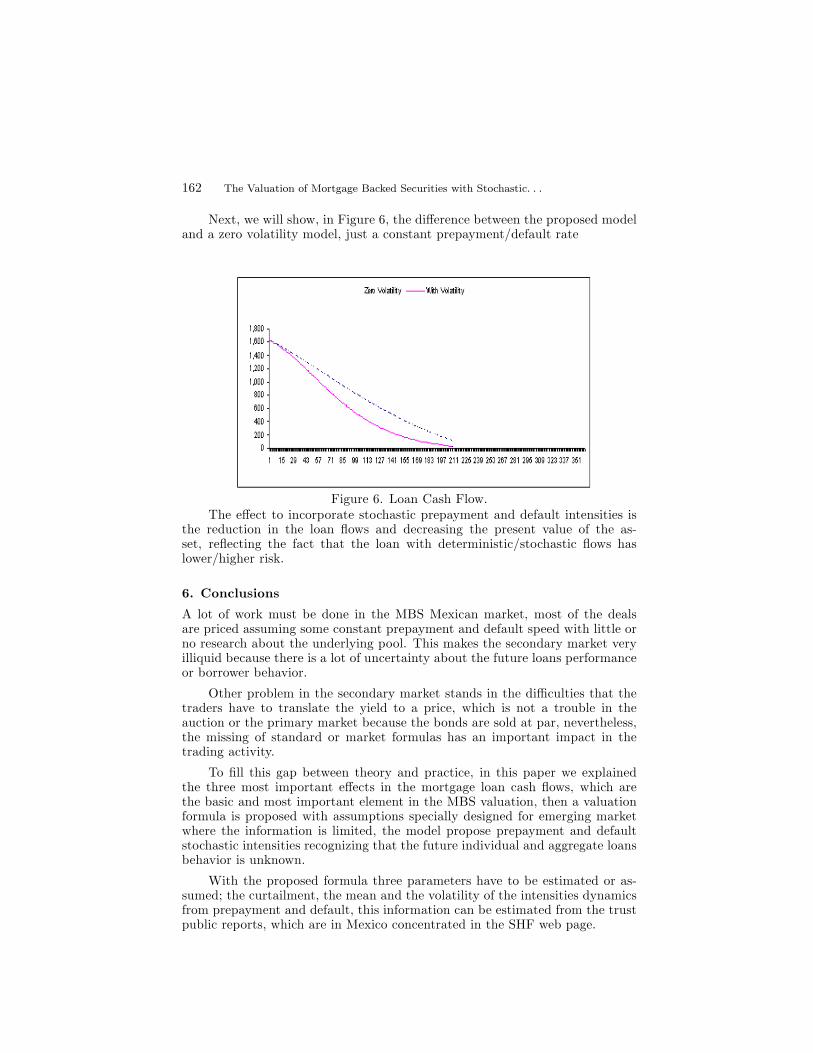
Next, we will show, in Figure 6, the di®erence between the proposed modeland a zero volatility model, j ust a constant prepayment/default rate

Figure 6. Loan Cash Flow.The e®ect to incorporate stochastic prepayment and default intensities is

the reduction in the loan °ows and decreasing the present value of the as-set, re°ecting the fact that the loan with deterministic/stochastic °ows haslower/higher risk.

6 . C o n c lu sio n s

A lot of work must be done in the MBS Mexican market, most of the dealsare priced assuming some constant prepayment and default speed with little orno research about the underlying pool. This makes the secondary market veryilliquid because there is a lot of uncertainty about the future loans performanceor borrower behavior.

Other problem in the secondary market stands in the di±culties that thetraders have to translate the yield to a price, which is not a trouble in theauction or the primary market because the bonds are sold at par, nevertheless,the missing of standard or market formulas has an important impact in thetrading activity.

To ¯ll this gap between theory and practice, in this paper we explainedthe three most important e®ects in the mortgage loan cash °ows, which arethe basic and most important element in the MBS valuation, then a valuationformula is proposed with assumptions specially designed for emerging marketwhere the information is limited, the model propose prepayment and defaultstochastic intensities recognizing that the future individual and aggregate loansbehavior is unknown.

With the proposed formula three parameters have to be estimated or as-sumed; the curtailment, the mean and the volatility of the intensities dynamicsfrom prepayment and default, this information can be estimated from the trustpublic reports, which are in Mexico concentrated in the SHF web page.

F ra n cisco V en eg a s-M a rt¶³n ez y J . V icto r R ey n o so -V en d rell 163

In the last section we show an example of the implementation of the model,the cash °ows can be easily calculated with very limited information from thepool. The model adj ust these future °ows to the uncertainty involve, re°ectingthe fact that the loan with deterministic/stochastic °ows has lower/higher risk.

A p p e n d ix 1

Proof of formula (26) .

We start with the general formula (24) :

E[F lo w (t)j= s ] = E [(P M T (t) + ¿ (t) (B (t¡ ) ¡ (P M T (t) ¡ I O (t) ) )

+B (t) ¸ P (t) ) S D (t) S P (t¡ )j= s¤ (A :1)

We assume that the intensities have the following dynamics:

d ¸ P (t) = ¹ ¸ P d t + ¾ ¸ P d W (t); (A :2)

d ¸ D (t) = ¹ ¸ D d t + ¾ ¸ D d W (t); (A :3)

d W d ¹W = ½ d t; (A :4)

After computing the expected value the stochastic process, we have:

E[F lo w (t)j= s ] = P M T (t) + ¿ (t) (B (t¡ ) ¡ (P M T (t) ¡ I O (t) ) )

E£S D (t) S P (t¡ )j= s

¤+ B (t) E

£¸ P (t) S D (t) S P (t¡ )j= s

¤ (A :5)

The ¯rst expected value in the above equation satis¯es:

E£S D (t) S P (t¡ )j= s

¤= E

·exp

µ¡Z t

s

¸ D (u )d u

¶exp

µ¡Z t¡

s

¸ P (u )d u

¶j= s¸;

(A :6)or

E£S D (t)S P (t¡ )j= s

¤= E

·exp

µ¡Z t

s

¸ D (u )d u

¶j= s¸

E

·exp

µ¡Z t¡

s

¸ P (u )d u

¶j= s¸

+ Cov¡S D (t)S P (t¡ )j= s

¢:

(A :7)The solution of the ¯rst two expected values in equation (A :7) are well knownin the interest rate literature, see Nielsen (1999) . For the covariance we have:

Cov¡S D (t) S P (t¡ )j= s

¢= ¾ S D (t) ¾ S P (t)½ S D S P : (A :8)

Then, we need to compute the variance of S D and S P , the solution is the samefor both so we will j ust show for default:

Var

·exp

µ¡Z t

s

¸ D (u )d u

¶j= s¸

= E

"

exp

µ¡Z t

s

¸ D (u )d u

¶2j= s

#

¡ E

·exp

µ¡Z t

s

¸ D (u ) d u

¶j= s

2: (A :9)

164 T h e V a lu a tio n o f M o rtg a g e B a ck ed S ecu rities w ith S to ch a stic:::

If 0 · s · t, then

¸ D (t) =¡¸ D (s ) + ¹ ¸ D (t ¡ s ) + ¾ ¸ D ( ¹W (t) ¡ ¹W (s ) )

¢; (A :10)

E

·exp

µ¡Z t

s

¸ D (u ) d u

¶j= s¸

= E

·¡Z t

s

¡¸ D (s ) + ¹ ¸ D (u ¡ s ) + ¾ ¸ D ( ¹W (u )

¡ ¹W (s ) )¢d u j= s

¤:

(A :11)

E

·exp

µ¡Z t

s

¸ D (u ) d u

¶j= s¸

= E

·exp

µ¡µ

¸ D (s ) +1

2¹ ¸ D (t ¡ s )

¶(t ¡ s )

¡Z t

s

¾ ¸ D ( ¹W (u ) ¡ ¹W (s ) )

¶d u j= s

¸ :

(A :12)The only stochastic element in the above equation is the following integral:

E

·Z t

s

( ¹W (u ) ¡ ¹W (s ) ) d u j= s¸

=

Z t

s

E£

( ¹W (u ) ¡ ¹W (s ) )j= s¤d u = 0: (A :13)

Then, we have that the mean and variance of (A :13) are:

E

·¡µ

¸ D (s ) +1

2¹ ¸ D (t ¡ s )

¶(t ¡ s ) ¡

Z t

s

¾ ¸ D ( ¹W (u ) ¡ ¹W (s ) )

¶d u j= s

¸=

¡µ

¸ D (s ) +1

2¹ ¸ D (t ¡ s )

¶(t ¡ s ) ;

(A :14)

Var

·¡µ

¸ D (s ) +1

2¹ ¸ D (t ¡ s )

¶(t ¡ s ) ¡

Z t

s

¾ ¸ D ( ¹W (u ) ¡ ¹W (s ) )

¶d u j= s

¸=

¾ 2¸ D Var

·Z t

s

(t ¡ u )d ¹W (u )j= s¸;

(A :15)

Var

·¡µ

¸ D (s ) +1

2¹ ¸ D (t ¡ s )

¶(t ¡ s ) ¡

Z t

s

¾ ¸ D ( ¹W (u ) ¡ ¹W (s ) )

¶d u j= s

¸=

¾ 2¸ D

3(t ¡ s ) 3 :

(A :16)Finally, we have that the exponential of a random normal distributed variablewith mean (A :15) and variance (A :16) is:

E

·exp

µ¡Z t

s

¸ D (u ) d u

¶j= s¸

= exp

µ¡µ

¸ D (s ) +1

2¹ ¸ D (t ¡ s )

¶(t ¡ s )

+¾ 2¸ D

6(t ¡ s ) 3 :

:

(A :17)

F ra n cisco V en eg a s-M a rt¶³n ez y J . V icto r R ey n o so -V en d rell 165

and the expected value of the square of S D is:

E

·exp

µ¡ 2

Z t

s

¸ D (u ) d u

¶j= s¸

= exp

µ¡ 2

µ¸ D (s ) +

1

2¹ ¸ D (t ¡ s )

¶(t ¡ s )

+2¾ 2¸ D

3(t ¡ s ) 3 :

:

(A :18)Hence, the variance of S D is:

Var

·exp

µ¡Z t

s

¸ D (u )d u

¶j= s¸

=

µexp

µ2¾ 2¸ D

3(t ¡ s ) 3

¶

¡ exp

µ¾ 2¸ D

3(t ¡ s ) 3

¶¶exp

µ¡ 2

µ¸ D (s ) +

1

2¹ ¸ D (t ¡ s )

¶(t ¡ s )

¶:

(A :19)

Var

·exp

µ¡Z t

s

¸ D (u ) d u

¶j= s¸¼µ

¾ 2¸ D

3(t ¡ s ) 3

¶

µ¡ 2

µ¸ D (s ) +

1

2¹ ¸ D (t ¡ s )

¶(t ¡ s )

¶;

(A :20)

¾ S D (t) ¼ exp

µ¡ 2

µ¸ D (s ) +

1

2¹ ¸ D (t ¡ s )

¶(t ¡ s )

¶¾ 2¸ Dp

3(t ¡ s ) 3 = 2 : (A :21)

If the volatility is small, then

Cov¡S D (t)S P (t¡ )j= s

¢= ¾ S D (t) ¾ S P (t)½ S D = S P ¼ 0; (A :22)

and equation (A :5) is approximately:

E[F lo w (t)j= s ] ¼ P M T (t) + ¿ (t) (B (t¡ ) ¡ (P M T (t) ¡ I O (t) ) )

E£S D (t)j= s

¤E£S P (t¡ )j= s

¤+ B (t) E

£¸ P (t)S D (t)S P (t¡ )j= s

¤

(A :23)With similar arguments, we can see that the second part of the equation alsohas covariance close to zero:

E£¸ P (t) S D (t) S P (t¡ )j= s

¤=E

£¸ P (t)j= s

¤E£S D (t) S P (t¡ )j= s

¤+

Cov£¸ P (t) ;S D (t) ;S P (t¡ )j= s

¤;

(A :24)

and if the volatility of prepayment is small then:

Cov£¸ P (t) ;S D (t);S P (t¡ )j= s

¤= ¾ ¸ P ¾ S D ;S P ½ ¼ 0; (A :25)

E£¸ P (t)S D (t)S P (t¡ )j= s

¤=E

£¸ P (t)j= s

¤E£S D (t)j= s

¤E£S P (t¡ )j= s

¤;

(A :26)where

E£¸ P (t)j= s

¤=¸ P (s ) + ¹ ¸ P (t ¡ s ) : (A :27)

166 T h e V a lu a tio n o f M o rtg a g e B a ck ed S ecu rities w ith S to ch a stic:::

Thus, the expected value of both survival probabilities is given by

E£S D (t)j= s

¤E£S P (t¡ )j= s

¤=E

·exp

µ¡Z t

s

(¸ ¤ (s ) + ¹ ¤ (u ¡ s ) + ¾ ¤ (W ¤ (u )

¡ W ¤ (0) ) ) d u

¶j= s¸;

(A :28)with

¸ ¤ (s ) = ¸ P (s ) + ¸ D (s ) ;

¹ ¤ = ¹ ¸ P + ¹ ¸ D ;

¾ ¤ =q

¾ 2¸ P

+ ¾ 2¸ D

+ ½ ¾ ¸ P ¾ ¸ D :

The solution of the (A :28) expected value is (see Nielsen, 1999) :

E£S D (t)j= s

¤E£S P (t¡ )j= s

¤=P (¸ ¤ (s );t ¡ s )

(A :29)

P (¸ ¤ (s ) ;t¡ ¡ s ) = exp

µ¡ ¸ ¤ (s ) (t¡ ¡ s ) ¡ 1

2¹ ¤ (t¡ ¡ s ) 2 +

¾ ¤ 2

6(t¡ ¡ s ) 3

¶;

(A :30)

F ra n cisco V en eg a s-M a rt¶³n ez y J . V icto r R ey n o so -V en d rell 167

A p p e n d ix 2

Month Number of Credits Prepayment Default (90+ DaysDelinquency)

11-2003 1979 8 012-2003 1971 7 301-2004 1964 8 002-2004 1956 10 303-2004 1946 12 404-2004 1934 10 405-2004 1924 10 406-2004 1914 8 507-2004 1906 11 608-2004 1895 7 409-2004 1888 10 510-2004 1878 11 511-2004 1867 10 1012-2004 1857 10 601-2005 1847 9 702-2005 1838 12 303-2005 1826 8 1004-2005 1818 10 505-2005 1808 13 806-2005 1795 9 807-2005 1786 19 608-2005 1767 17 709-2005 1750 9 710-2005 1741 11 1111-2005 1730 10 512-2005 1720 14 601-2006 1706 11 202-2006 1695 9 603-2006 1686 15 704-2006 1671 12 605-2006 1659 11 606-2006 1648 19 1007-2006 1629 9 708-2006 1620 11 809-2006 1609 17 510-2006 1592 8 911-2006 1584 13 1012-2006 1571 11 701-2007 1560 19 3

168 T h e V a lu a tio n o f M o rtg a g e B a ck ed S ecu rities w ith S to ch a stic:::

R e fe r e n c e s

Andersen, Per Kragh, Borgan, O. , Gill, Richard D. , Keiding, Niels. , (1993) .Statistical Models Based on Counting Process, Springer-Verlag New YorkInc.

Davidson, A. , Sanders, A. , Wol®, Lan-Ling, Ching, A. , (2003) . Securitization,Structuring and Investment Analysis, John Wiley & Sons, Inc. , Hoboken,New Jersey.

Fabozzi, Frank, J. , (2006) . The Handbook of Mortgage Backed Securities, 6thedition, McGraw-Hill.

Hastie, T. , Tibshirani, R. , (1986) . Generalized Additive Models, StatisticalScience, Vol. 1 , No. 3, 297-318.

Nielsen, T. L. , (1999) . Pricing and Hedging of Derivative Securities, OxfordUniversity Press.

SchÄonbucher, Philipp, J. , (2003) . Credit Derivatives Pricing Models, JohnWiley & Sons Ltd.

The Bond Market Association, (2000) . Standard Formulas for the Analysis ofMortgage-Backed Securities and Other Related Securities. TBMA, NewYork.

Rebonato, R. , (2002) . Theory and Practice of Model Risk Management. Quan-titative Research Center.

Venegas-Mart¶³nez, F. , (2006) . Riesgos Financieros y Econ¶omicos, InternacionalThomson.