THE USE OF THE NASM II I GEODIMETER

BY THE SOUTH ATLANTIC HYDROGRAPHIC MISSION

by Paul P l o u v ie z

Ingénieur Hydrographe Principal French Navy Hydrographic Service

1.1. — The aim of this article is neither to expose the theoretical consi­derations of the NASM III geodimeter, nor to give a detailed report of geodetic surveys carried out, but rather to allow the users of this instrument to profit from the experience acquired by the French Navy Hydrographic Service of which the Mission Hydrographique de VAtlantique Sud (M. H. A. S.) (South Atlantic Hydrographie Mission) measured more than 100 distances during two seasons, i.e. during a total of about 7 months. The following points will be studied in detail : ground equipment for geodetic traversing, adjustment of the geodimeter, method of operation, theoretical and practical accuracy of the instrument, maximum range obtained, cali­bration, instrument failures and desirable improvements in the geodimeter and its method of use. The instruction book on the instrument, although very detailed, does not in fact give all the instructions on the field adjust­ments of the geodimeter, or on the instrument’s accuracy limit under intensive use.

1.2. — The French Navy Hydrographic Service wished to carry out accurate geodetic work on the Gabon and Congo coasts between Cap Lopez and the region of Pointe-Noire, i.e. over about 600 km. The reconnaissance, setting-up and observations of a triangulation chain of the first or second order in this area covered with forests, cut up by numerous branch channels of rivers and devoid of means of communication, would have raised consi­derable difficulties. Very often it would have been necessary to use B il b y

metal towers which would have required considerable means of transport and a specialized personnel for the erection and dismantling of the towers. A much more rapid and economical solution was to carry out on the coastal area, along which one can move more easily, a high precision geodetic traverse. This recent technique is possible only if one has available an instrument allowing very rapid measurement of distances from 10 to 150 km with an accuracy of the order of 1-10-5. Coastal hydrography requires, in fact, a geodetic net with density of stations along a line as opposed to the cartography of a country which requires a geodetic net covering the entire surface to be represented. The M. H. A. S. having received in August 1957 a NASM III geodimeter, and the geodetic work between

Pointe-Noire and Cap Lopez being planned for 1958, it was decided to carry out a precision geodetic traverse along the coast, the distances being measured with the geodimeter and the angles with a Wild T3 theodolite.

2. — Plan of M. H. A. S. geodetic operations in 1958 and 1959

(figure 1)

The work was undertaken with the co-operation of the Société Française

des Pétroles de l’Afrique Equatoriale (S. F. P. A. E.). The immediate object- tive was to determine the positions of the antennas of a mobile Toran radio­positioning chain, (hyperbolic system) installed to carry out gravimetry and marine seismic studies, as well as the regular survey of the sea bottom.

During the first season from August to October 1958, the land was marked out between Cap Lopez and the village of Tassi situated 175 km to the south; the first 155 kilometres were surveyed during the same period, the last 20 were done in June 1959.

The second survey, from April to September 1959, took place in the region extending from Pointe-Noire to Mayumba where a traverse 220 km long was marked out and surveyed. In this area there existed only a small triangulation chain extending for 30 km north of Pointe-Noire.

During these surveys, the traverses were re-oriented about every 50 km by azimuth observations of the stars.

3. — Lessons from geodetic surveys

3.1. — Ground equipment

The first condition for carrying out a precise geodetic traverse is to construct ground marks, the centres of which are perfectly defined and on which the instrument can be set up. The NASM III geodimeter weighs about 20 kg and requires the same stability as a theodolite.

It can be set up either on a special tripod, resting on the ground, or on a geodetic pillar, using three short feet designed for attachment to the geodi­meter under its base-plate. The geodetic pillar should have a platform measuring at least 40 cm X 40 cm.

Geodimeter measurements can be carried out only if there is a clear line-of-sight, as for a theodolite’s line-of-sight. It is necessary therefore that the line-of-sight should be well clear of vegetation in order to avoid all absorption of light by grass or brush. The best way of providing ground facilities of a lasting kind is to build stone pillars several metres high.

During the 1958 season, pillars of reinforced cement were built on the site; they were three metres high with a cross-section of 40 cm by 40 cm. The foundation consisted of a solid mass 1 metre deep, surmounted by a flagstone 150 X 150 X 20 cm. An independent wood platform was built around the pillar for the observers (figure 2).

In 1959, profiting from the experience of the 1958 season which proved

that the on-site construction of the pillar was a heavy burden from a logistic point of view and that stability was more than ample, another type of pillar was adopted. The new type of reinforced concrete pillar was prefabri­cated at Pointe-Noire; it was 4 metres long with a cross-section of 27x27 cm. The pillar was transported by lorry and placed in a concrete mass of about one-half a cubic metre which was moulded on site; a flagstone of 40 X 40 cm was added to the pillar to support the geodimeter. An independent platform was constructed around the pillar. This very much lighter type of pillar gave complete satisfaction from the point of view of stability.

3.2. — Personnel and material requirements

Three persons are required for carrying out geodimeter measurements : 1 observer and his assistant who carry out the measurement on the geodi­meter, and an assistant at the other end of the distance to be measured, who is charged with the orientation of the reflector and lighting the projec­tor used for sighting the geodimeter. The observer can, if necessary, operate alone but this increases the time taken for the measurement and detracts from its accuracy as will be shown further on.

The ideal means of transport in a country without roads, and consider­ing the small bulk of the instruments being transported, was a light over­land vehicle. The geodetic team was composed of 4 men; in 1958 they were equipped with one vehicle; in 1959, a second vehicle and reflector for the geodimeter allowed the team to double its efficiency.

3.3. — Adjustment of the geodimeter

The geodimeter is a device which necessitates considerable care in the adjustments, as measurements are not possible unless all the adjustments have been correctly carried out. The NASM III device, delivered directly to the Mission from the manufacturer, could function only after it had been found that a certain number of adjustments were necessary in the optical part.

3.3.1. — O p t ic a l a d ju st m e n t

The optical adjustment should be carried out according to the instruc­tion book; as a rule these adjustments are stable for the most part, except if the geodimeter receives a shock or if, following the replacement of the projection lamp, the optical path is modified. The adjustments which, on the contrary, must be carried out for practically each measurement are :

— position screw of the projection lamp;— vertical and horizontal adjustment screw of the small transmitting

mirror;— vertical and horizontal adjustment screw of the small receiving

mirror.

We shall explain the M. H. A. S. adjustment methods which have given complete satisfaction.

3.3.1.1. — Adjustment of the spherical transmitting mirror

a) Operate in darkness; light the projection lamp with the tetrapode in place and verify that the ring of light sent back by the small mirror on to the large mirror is absolutely centred. A small graduated white rule, placed on the large mirror, is used for this. If not adjusted, the adjustment of the horizontal and vertical screws of the small transmitting mirror must be made again.

b) Next obtain the same point on the centre of the Kerr cell’s plates when sighting a distant point with or without the tetrapode, by again making the adjustment of the screws of the large mirror.

3.3.1.2. — Adjustment of the receiving optical section

It is more advantageous to operate with a powerful projector situated at a great distance and directed towards the geodimeter, previously brought to bear on the projector. The geodimeter is then adjusted in conditions identical to its conditions of use; we have ascertained that this adjustment is preferable to the one described in the instruction book.

Remark

In our opinion it is advisable to mark each of the four feet of the geodimeter in a different manner so that they are always remounted at the same place. Thus modifications of the optical path due to the tetrapode should be avoided if slight differences exist between the four feet.

3.3.2. — E l e c t r o n ic a d j u s t m e n t s

The electronic part of the geodimeter is, on the whole, much more stable, with the reservation of some precautions which we shall enumerate further on.

3.3.2.1. — Equalization of phases 1 and 2

This equalization is accomplished by means of the lamp’s position- moving screw, the instrument functioning on the optical calibration path, and having been under voltage for at least 10 minutes, so that thermal equilibrium is attained. This adjustment must be made again for practi­cally each measurement.

3.3.2.2. — Equalization of phases 2 and 3

This adjustment does not have to be repeated very often. Nevertheless we shall note the manner of carrying it out as it is not indicated in the instruction book and too great an inequality between phases 2 and 3 could prevent the taking of measurements.

When the light is off, the delay line being out of use and the high voltage being in use, adjust the zero-indicator to 0 by means of the zero adj knob; then adjust the potentiometer P3 to equalize phases 2 and 3.

Only an adjustment area, and not a single position for P3, can be obtained. Then connect an electronic voltmeter with the grids of the two tubes of the zero detector and adjust P3 to obtain about 50 mV. The position

obtained should be located in the middle of the limits previously defined. If not, check the values of the resistance bridge of which P3 is a part.

3.3.2.3. — In addition to these adjustments, it may be necessary to re-tune the oscillating circuits of frequencies Fx and F2, when Fx and F2 measurements are not equally sensitive.

Finally, when large variations are noted in the delay line, it becomes necessary to re-adjust its tuning.

3.3.2.4. — Protection of the electronic part

The delay line and the photoelectric cell unit are very sensitive to humidity and are placed in insulated casings dried by silicagel cartridges.

A lack of protection of the delay line could modify its constants. If the casing of the phototube is not perfectly dry, the lost current is too great and the sensitivity is insufficient for carrying out measurements. In parti­cular, the indication of the measuring device in position 4 is 1.8 when the cell and the light are off. When the cell is under voltage, the indication should not go below 1.4 to 1.3; finally, when the light is received, the indication falls to 0.7-0.9. If the silicagel cartridge needs to be recharged, the polarization voltage is markedly weaker and measurements are impos­sible. A drop in voltage greater than 5 divisions corresponds to a lost current which is too large.

3.4. — Method of use

There is no question of going over again the instructions given in the instruction book of the instrument, but rather of giving some details which appear useful to us.

3.4.1. — O p t ic a l s ig h t in g a n d a d j u s t m e n t

To sight the instrument we used a projector made of a special auto­mobile head-lamp producing a cylindrical beam. If the optical section has been suitably adjusted, and the geodimeter, without the tetrapode, sighted very carefully, once the tetrapode is in place there should be no further reason to touch the sighting unless it is to perfect it. Verify the adjustment of the small transmitting mirror with respect to the large mirror.

The sighting having been carried out, when the beam of non-polarized light is projected to the reflector placed at a great distance, the beam reflected by the reflector should be seen by an observer standing in front of the receiving part of the geodimeter. If this does not occur, the optical transmission section is out of adjustment. The adjustment of the optical reception section is made as explained in sub-section 3.3.1.2. As a rule, this adjustment does not often need to be made.

Remark

When looking through the optical part of the geodimeter, one should perceive the filament of the lamp centred between the plates of the Kerr cell.

3.4.2. — E l e c t r o n ic a n d o p t ic a l a d j u s t m e n t s

As a result of the interdependence of optical phenomena, it may become necessary again to make certain of the optical adjustments during the following phase of the focussing.

Set the needle of the zero-indicator at 0 by means of the adj knob; this adjustment should remain with phases 1, 2, 3 and 4; if not, it may become necessary again to make the adjustment of the P3 potentiometer.

Equalize phases 1 and 2 using the interior optical path with polarized light, as explained in sub-section 3.3.2.1.

Next, the adjustment of the transmission and reception optical sections should be finished, using the long distance reflector. This is the most deli­cate adjustment for it requires a certain amount of training and adroitness.

The light beam being polarized, the diaphragm is opened gently, having brought the delay line into use by engaging one of the studs. The needle of the zero-indicator should then deviate when the delay line studs are successively engaged. The deviation will moreover be more rapid, all things equal, as the engaged stud is farther removed from the stud producing equilibrium. The most delicate and most frequent case appears when the receiving-end sensitivity is practically nil; the operator’s entire art is to increase the sensitivity. This is done by touching slightly the vertical and horizontal screws as well as the focal length of the small receiving mirror, and the vertical and horizontal screws of the small transmitting mirror. One must remember that as a rule the correct adjustments are very close and that, in general, it will require very little to increase the sensitivity.

Maximum sensitivity corresponds to the equality of phases 1 and 2; this equalization is obtained by modifying the vertical and horizontal adjustment screws of the small transmitting mirror. It must be noted that, for this required adjustment, the adjustment of each of the two screws is the middle adjustment in the centre of the adjustment area between the limits of which the observer is seeing the maximum light with a non­polarized beam, when standing in front of the receiving mirror.

The adjustments of the transmission and reception mirrors not being independent, as soon as one obtains sufficient sensitivity, phases 1 and 2 must be equalized, and then the maximum sensitivity must be sought by adjusting only the optical reception.

Let us note that the equalization of phases 1 and 2 is increasingly sensitive to the dissymmetry of the beam and, in consequence, to the position of the lamp filament, as the homogeneousness of the nitrobenzine of the Kerr cell is defective. It may be necessary to adjust the phototube position. Nevertheless, once done, this adjustment need not be repeated because the optimium position is between the limits of an area. It is therefore in our interest to seek the centre of this area in the course of a measurement when the sensitivity is good, and not touch this adjustment afterwards.

3.4.2.1. — Method of using the instrument

The above adjustments having been carried out, we may then begin the measurement as described in the intrument’s instruction book. We shall mention however a certain number of essential points.

3.4.2.2. — Adjustment of zero adj and delay adj knobs

When carrying out a distance measurement on one of the frequencies, it is important to set the needle of the zero-indicator at 0 with the zero adj knob, the studs of the delay line being out of use. It is very important not to touch the delay adj knob again for the duration of the Fx or F2 mea­surements because this knob shifts the zero of the fine readings scale.

3.4.2.3. — Calibration of the fine scale

This calibration is used to determine the value of one division of the fine scale, by carrying out a measurement on the interior optical path with studs “ 50 ” and “ 45 ”. We shall note that if the fine readings difference between the measurement on the reflector and on the interior optical path wTith stud “ 0 ”, is small, i.e. of the order of 10 to 15 divisions, it is unnecessary to make this calibration. The value of one division has a mean value of the order of 11 cm and its variations rarely exceed 2 to 3 % .

We can therefore begin the measurement in the order : “ 0 ” calibra­tion, measurement on the reflector, “ 0 ” calibration; the fine scale calibra­tion will be carried out afterwards if the fine reading is large.

3.4.2.4. — Zero shift

The zero shift becomes smaller as the measurements are carried out more rapidly; it is important therefore that all adjustments be made before beginning the calibration on the interior optical path with stud “ 0 ”. Once the measurements on the reflector are made, a final calibration must be carried out immediately afterwards. The means of the 4 measurements on the interior optical path should not differ by more than 0.5 division, or the zero shift is too large; in general, these values do not differ more than 0.1 to 0.2 division.

3.4.2.5. — Tuning of Kerr cell

The Kerr cell tuning must be made again for each measurement; we decrease this tuning with the measuring device at position 7; then we finish in position 4 with the delay line in operation. The imperfection of the delay line can in fact slightly modify the tuning.

3.4.3. — S ig h t in g w i t h o u t a s s is t a n c e

The Mission successfully experimented with a method of sighting the geodimeter which necessitates no assistance. For this, the transmitting and receiving sections of the geodimeter must be in adjustment. An automobile head-lamp beam is then projected in the direction of the reflector which sends back the light, after which the geodimeter may be sighted as described in sub-section 3.4.1.

3.4.4. — U s e o f s e v e r a l r e f l e c t o r s

When one has to carry out a measurement under bad visibility condi­tions or at the range limit of the instrument, it is in one’s interest to add a second, or even a third, reflector. The base-plate of the reflector was designed to take three; the orientation of the prisms, which should always have their references towards the top, must then be re-established.

3.5. — Theoretical accuracy

3.5.1. — C a u s e s o f e r r o r s

The distance measured by the geodimeter is given by the expression :

D = nx ui -f- dc -(- Lx (1)where :

nx is a whole number,

Ui the wave length on frequency Flt

dc the sum of the atmospheric corrections,

h 1 the total amount.

Li may be written :

L, = A, + (Fr — F„) • (2)*■45-^ 50

an expression in which Ax is the coarse amount, (Ax is a multiple of 5 between 0 and 50), its exact value being determined during calibration to within ± 3 cm. The second term of expression (2) is the fine amount. The F terms are the means of readings carried out on a variable condenser to within 0.5 division, by setting the galvanometer needle at zero. Therefore, there is a great similarity with the pointing of theodolites.

The Fr reading on the reflector is the mean of 8 readings.

The F0 reading on the interior optical path with stud “ 0 ” is the mean of 8 readings.

The F45 and F50 readings on the interior optical path with studs “ 45 ” and “ 50 ” are the means of 4 readings each.

Ago A45The fraction-------- represents the value of one division of the

F45 — f 50fine amount condenser at the moment of calibration.

The principal causes of errors are : the modulation frequency of the light intensity, the length of the delay line elements, atmospheric conditions and reading from the zero-indicator. Within a relatively short period, the first three errors are systematic; the last, random, may be reduced by increasing the number of readings.

3.5.2. — F r e q u e n c y

The value of the frequency is determined in a laboratory to within dr 2-10-6. Furthermore, the quartz of the oscillating circuit is closed in a thermostatically-controlled box and it is probable that the stability of the frequency corresponds to the precision with which its value is given.

3.5.3. — A t m o s p h e r ic c o n d it io n s

The speed of propagation of light, and consequently the wave length, vary with temperature, pressure and humidity conditions. A 1° error in

temperature or a 2 mm error of mercury in pressure results in an error of 110-6 in the wave length. The uncertainty of determination of atmos­pheric conditions may result in an error of 2-10-6 in the wave length.

3.5.4. — D e l a y l in e

The elements of the delay line are of a high electrical and mechanical stability; its variations due to ageing or change of temperature are negligible provided, however, that the enclosure of the delay line is suitably protected from humidity. Given this, the value of each of the delay line studs is determined by calibration with an uncertainty of ± 3 cm, taking into account both the precision of the measurement and the relative stability of the stud itself.

3.5.5. — Z e r o r e a d in g

When the measurement is carried out with a good level of reception one should have as much sensitivity in a measurement on the reflector placed at a great distance, as in a measurement on the interior optical path. In good conditions, readings can be made to within 0.5 division on the scale of the tine reading condenser. The zero readings serve on the one hand to determine the fine amount in numbers of divisions of the fine reading condenser : this is the quantity FR — F0; on the other hand, the value of one division of the fine reading condenser is determined by carrying out measurements on the interior optical path with studs “45 ” and “ 50 ”.

The quantity FB — F0, the difference of two means of 8 readings to within 0.5 division, introduces a mean square error of 0.25 division, i.e. 2.5 cm, since each division equals about 10 cm.

The quantity F45— F50, the difference of two means of 4 readings to within 0.5 division, introduces a mean square error of about 0.35 divi­sion; as F45— F50 has a mean value of 45 divisions, this represents an error slightly less than 1 %.

3.5.6. — F in e r e a d in g

The uncertainty of the value of a fine reading division has an influence on the value of the fine reading proportional to the number of divisions. The value of the division is subject to a systematic error due to the uncertainty with which is known the difference in length of studs “ 50 ” and “ 45 ”, i.e. the quantity A50 — A45, and also to a random error due to the fine reading calibration carried out each time the instrument is used.

The systematic error is about 1 %, assuming that each stud is known to within ± 3 cm. The random error is about 1 % (0.35 division of uncer­tainty on F45 — F50, which corresponds to 45 divisions).

3.5.7. — E s t im a t io n o f t h e o r e t ic a l a c c u r a c y

Let us first consider the case of a complete measurement on frequency Fx or F2 assuming that the distance is, for example, 10 km. The theoretical maximum errors due to different causes are :

Cause of error

Frequency ................................Atmospheric correction ..........Delay line stud .....................Fine reading (FR — Fc) ..........

Value of fine reading division :

Systematic part .......................

Random part ...................

Only the error on the delay line stud and a part of the fine reading division error are systematic.

The sum of the random errors has a maximum value of ± 10.5cm; this value is reduced to ± 6.5 cm when the fine reading is nil; the mean square value is ± 5.5 cm.

The total maximum error including both systematic and random errors is from ± 9.5 cm to ± 17.5 cm, depending on the value of the fine reading.

Let us now consider the case of a distance determined by the mean of measurements on frequencies Fj and F2. Generally a different delay line stud is used, and consequently, for the whole of the two measurements, the error is no longer systematic but random. The only systematic error remaining is the fine reading error.

If one considers the sum of the random errors, the mean square value is ± 6.5 cm for one measurement, i.e. for the mean of two measure­ments, ± 5 cm. The mean total error is therefore ± 4 cm ± 5 cm = ± 9 cm.

Let us note that the difference between the Fj and F2 measurements can be, at a maximum, from 19 to 26 cm; however the theory of errors gives ± 12 cm as a mean figure. In the case of a rectilinear traverse of yj ranges,

the total error would be : 5\/rj cm -f 4 yj cm.

3.5.8. — R e l ia b il it y

The elements liable to variation are : the modulation frequency of light, the delay line elements and the fine amount circuit. The frequency should not vary more than 2 10-6 and, if the drying of the delay line is suitably assured, it should not vary. On the other hand, the fine amount circuit appears to be subject to rapid variations; for this reason the manufacturer recommends calibration of this circuit for each measurement. In theory, the geodimeter should be a reliable instrument; two measurements of the same distance carried out with an interval of several months should not differ by more than 13 to 21 cm (according to the fine reading value), the mean values being 7 to 12 cm.

Observation Error in cm

random ± 2random ± 2

systematic ± 3random ± 2.5

The fine reading varies from 0 to

45 divisions, ± 4

The error variesfrom 0 to 4 cm ± 4

3.6. — Calibration

3.6.1. — The calibration of the geodimeter should include on the one hand, measurements of short distances allowing the determination of the value of each delay stud, and on the other hand, distance measurements over large geodetic bases whose length is known with great precision in order to ascertain that the frequency of the geodimeter has not varied too much.

We shall add also a word on short distance calibration carried out immediately after a long distance measurement for which high accuracy is desired and which will allow the combined calibration of the stud and fine amount of the measurement.

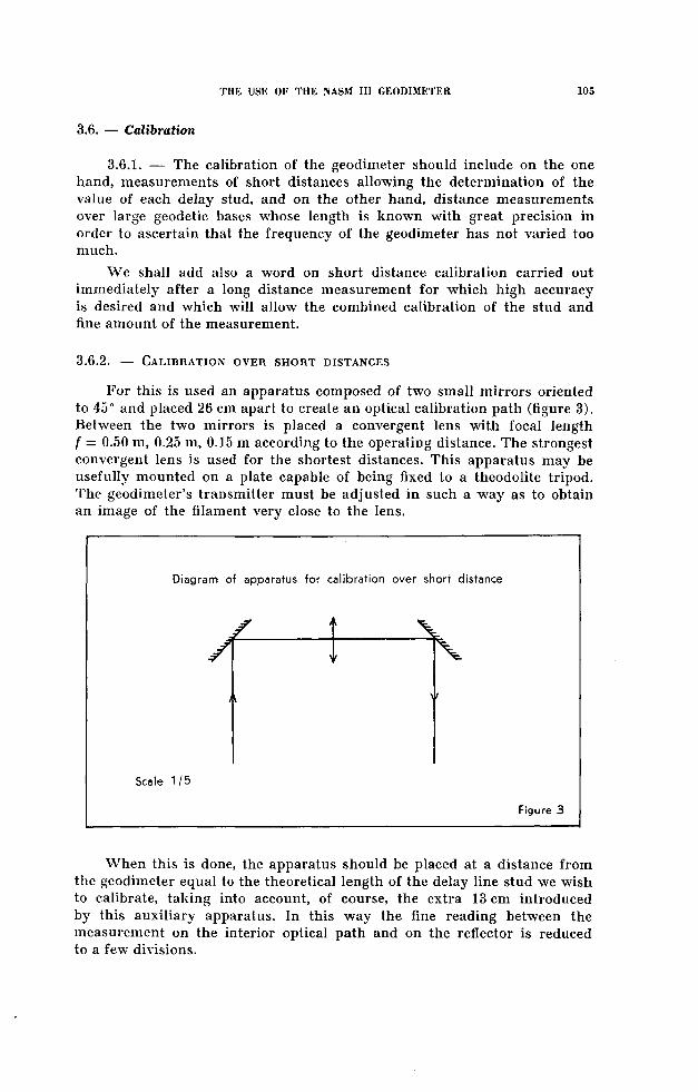
3.6.2. — Ca l ib r a t io n o v e r s h o r t d ist a n c es

For this is used an apparatus composed of two small mirrors oriented to 45° and placed 26 cm apart to create an optical calibration path (figure 3). Between the two mirrors is placed a convergent lens with focal length f = 0.50 m, 0.25 m, 0.15 m according to the operating distance. The strongest convergent lens is used for the shortest distances. This apparatus may be usefully mounted on a plate capable of being fixed to a theodolite tripod. The geodimeter’s transmitter must be adjusted in such a way as to obtain an image of the filament very close to the lens.

Diagram of apparatus for calibration over short distance

Scale 1/5

Figure 3

When this is done, the apparatus should be placed at a distance from the geodimeter equal to the theoretical length of the delay line stud we wish to calibrate, taking into account, of course, the extra 13 cm introduced by this auxiliary apparatus. In this way the fine reading between the measurement on the interior optical path and on the reflector is reduced to a few divisions.

In this manner the stud is calibrated with a maximum error of ± 2.5 cm. It will be necessary to carry out two successive measurements and to ascertain that the results do not differ by more than 2.5 cm from one another, the only measurement error being that committed in the deter­mination of Fr — F0, i.e. 0.25 division.

3.6.3. — R e su lt s o f stud c a l ib r a t io n

The geodimeter’s delay line had been calibrated at the factory in June1957 and then by the Mission in October 1958, March 1959, September 1959, December 1959, March 1960 and June 1960. The curves showing the variations in length of the delay line with respect to the initial values are given in figure 4. It is noted that from October 1958 to June 1960, the value of each stud of the delay line varied within limits of about 10 cm.

3.6.4. — Ca l ib r a t io n o v e r lo n g d ist a n c e s

We cannot hope to determine, with the help of a series of measurements on a large base, if the unit of the geodimeter wave length is correct. In fact, it is defined to within ± 2 10-6 which corresponds to 2 cm for a 10- kilometre measurement. We have seen that the accuracy of a geodimeter measurement is of order of 10 cm without precautions, therefore, we cannot note through this process discrepancies lower than from 1 to 2 • 10-6.

The manufacturer recommends that, immediately after the measure­ment, a calibration should be carried out of the total amount over a short distance (coarse amount increased by fine amount). To this end, the total amount Llf which was found by measurement of distance D, should be

computed. We shall find a fine amount which will differ by a small number of divisions from the fine amount found during the long distance measure­ment. The total amount provided by the long distance measurement will be corrected by this difference.

Operating in this manner and subject to the stability of the fine amount circuit between the measurement and the calibration carried out soon afterwards, two causes of errors are eliminated : the coarse delay error and the calibration error of one fine reading division; there finally remains the whole error of one calibration, i.e. ± 2.5 cm.

Operating thus on a 10 km distance measurement carried out on one of the frequencies, the maximum errors may be reduced to :

Frequency......................................................... ±2 cmAtmospheric conditions ................................ ±2 cmZero reading error (FR — F0) ..................... ±2.5 cmCalibration error of total am oun t................. ±2.5 cm

That is, a maximum error of ± 9 cm and a mean square error of ± 4.5 cm. Operating in this manner we can hope to detect frequency discrepancies of the order of 1-10~5.

3.6.5. — R esu lt s o f c a l ib r a t io n o v e r t h e bases

The geodimeter was successively calibrated on the Tiaroye base on the Cap Vert peninsula and on the two Brazzaville bases.

Pate Frequency DistanceBaselength

Upper lim it of possible

error

Divergence from value

of base

19- 4-58 F ! 5878. 38 5878.57 ± 13. 5 - 19

IIF 2 5878. 27 II ± 13. 5 - 30

17-12-58 Fx 5878. 55 11 ± 13. 5 - 2

17- 4-59 F 1 5878. 54 11 ± 7* - 3

IIf 2 5878. 52 I I ± 12. 5 - 5

9- 9-59 F ! 3122. 46 3122. 29 ± 7* + 17

IIF i 3122. 37 i i

± 7* + 08

I IF 2 3122. 42 i i ± 7* + 13

11F2 3122. 37 i i

± 7* + 08

13- 9-59 F ! 3122. 25 i i ± 11 + 04

i tF 2 3122. 37 i i ± 8 + 08

11- 9-59 Fx 5258. 33 5258. 21 ± 13,5 + 12

hF 2 5258. 19 i i ± 7* - 02

(*) Measurement with calibration over short distance.

Taking into account these results and the upper limit of the error of each measurement, we can admit that in September 1959, frequency Fj was too large by 3-10-5 and frequency F2 by 2-10-5. Nevertheless the correction has not been applied because these discrepancies could not be shown with certainty. The aberrant measurements of March 1958 are explained by the users’ lack of experience.

3.7. — Accuracy obtained during the 1958 and 1959 seasons

3.7.1. — D iv e r g e n c e b e t w e e n d is t a n c e m ea su rem en t s c a r r ie d o u t on

FREQUENCIES F ± AND F2

During the 1958 and 1959 seasons more than 100 distance measure­ments were made. The analysis of the divergences between the value given by frequency Fx and that given by frequency F2, gives a very good indica­tion of the relative accuracy of the geodimeter (figures 5 and 6).

1958 season — 38 measurements were carried out, the absolute value of the mean divergence is 9 cm; the mean divergence is — 1 cm which shows that the divergence between Fj and F2 measurements is purely random; 9 divergences are greater than 15 cm; the maximum divergence is 38 cm.

1959 season — 62 measurements were carried out, the absolute value of the mean divergence is 10cm; the mean divergence is — 1 cm; in this case as well the divergence between Fx and F2 measurements is purely random. 12 divergences are greater than 15 cm, but for 6 measurements we were able to find explanations of the origin of these large divergences. Finally 6 divergences greater than 15 cm remained unexplained, the largest divergence being 32 cm.

If we refer to the theoretical accuracy study, we see that for a measurement of 10 km, the maximum divergence between Fx and F2 mea­surements is 26 cm and that the mean square divergence is 12 cm. The theoretical accuracy estimation is completely justified by experience. Let us note that during the 1959 season, the coarse delay in five cases was the same for frequencies Fx and F2. Now in this case the delay stud error is the same for these two frequencies; we should then find the smallest divergence between Fx and F2 measurements. This was verified for distances of a mean of 5 km where the divergences were 0 cm, 2 cm, 5 cm, 11 cm and 0 cm.

3.7.2. — Cl o s u r e o f l o c a l t r ia n g u l a t io n n e t w o r k s

In the course of the work carried out in 1958, two verifications were made with triangulation points of the S. F. P. A. E. network. A closure was made on a traverse distance of 15 km comprising 5 bearings; it was about 1.60 m and approximately parallel to the traverse direction; the error calculated from the estimations made in sub-section 3.5.7. is about dt 30 cm. The discrepancy is about 1-10-4.

A second closure was made on a traverse distance of 100 km compri­sing 19 bearings. The closure is approximately parallel to the traverse

direction and is about 10 metres. The admissible error is ± 100 cm; the disagreement is 1-10-4.

We have therefore been able to show a difference of 1-10-4 between the lengths given by the geodimeter on the one hand and, on the other hand, by the steel tape used to measure the bases of the S.F.P.A.E.

During the work carried out in 1959 a verification was made with the triangulation in the Pointe-Noire region established in 1952 by the M.H.A.S. from a base measured by means of an invar rod. The closure on a distance of 27 km comprising 4 bearings is of the order of ± 26 cm; the discrepancy is about 1 -10—5.

3.7.3. — T ot a l len g t h o f t h e d e l a y l in e

When carrying out a measurement on the interior optical path with studs “ 0 ” and “ 50 ”, we may deduce from this measurement and from the values of studs “ 0 ” and “ 50 ”, the value of the wave length. If the delay line has not undergone a large variation, we should find exactly 50 metres by means of this computation. The accuracy of such a verification is 0.35 division, i.e. ± 4 cm.

During the 1958 season this verification was made 44 times (figure 7). The mean value obtained was 50.03 m, the mean divergence being 3.5 cm. During the 1959 season, the verification was made 41 times, taking into account the calibration of the studs at the beginning and at the end of the season (figure 8). The mean value was established as 49.92 m, the mean divergence being 3.5 cm. We were unable to find a satisfactory expla­nation for this value which differs markedly from the 50.00 m, which we should have found. It must be assumed either that the calibration errors of studs “ 0 ” and “ 50 ” were to be added, and this for the calibrations before and after the season, or that a systematic error of unknown origin was introduced by the instrument during this check.

3.7.4. — V a r ia t io n o f t h e v a l u e o f a f in e r e a d in g d iv is io n

During the 1958 season, fluctuations in the value of a fine reading division reached 2 to 3 %. The technicians of the AGA company when consulted also noted variations of this order and it appears that the fine reading circuit is subject to rapid variations.

In 1959 during the geodetic work, the calibration of the amount was made 39 times on frequency Fj and 37 times on frequency F2; the mean value found for each frequency being 0.111 m. The mean divergence was 0.14cm for Fx and 0.12 cm for F2, i.e. about 1 %.

The determination of the value of a division is made with an accuracy of the order of 1 %. The distribution of the values of the division is Gaussian (figure 9). If, therefore, the fine reading circuit varies, the value of the division oscillates about a fixed mean value.

3.7.5. — P r a c t ic a l r e l ia b il it y

A certain number of distances were measured with the geodimeter several times; the divergences noted for the measurements corresponding

to a same state of the delay line calibrated and suitably protected, have never exceeded 10 cm.

Date Distance Place Observation

March 1958 5878.38 Tiaroye base Frequency Fx

Dec. 1958 5878. 55If

Frequency Fx

March 1959 5878. 53M Mean of F2 and F2 measurements

9-9-1959 3122. 44 B razzav ille base Mean of 2 F1 measurements

9-9-1959 3122. 41tl Mean of 2 F2 measurements

13-9-1959 3122. 31It Mean of F̂ ̂ and F2 measurements

27-6-1959 2399. 09 One of the traverse sides

Mean of Fx and F? measurements

24-7-1959 2399. 12h Mean of F and F measurements

1 2

3.8. — Range

The theoretical range of the apparatus given by the manufacturer is 15 km; in Sweden, i.e. in excellent atmospheric conditions, the AGA technicians have reached 18 km. The range is limited by the adjustment of the optical section of the instrument, by the sighting of the instrument and by the adjustment of the electronic section. These adjustments having been made in the best way, the range will be better as the atmosphere becomes more transparent. In particular, the presence of a light mist or simply a humidity-laden atmosphere, will reduce the range.

In the course of the geodetic traverses, operating in bad visibility conditions (sides parallel to the beach, in the vicinity of a curtain of spray) 12 km was reached. We can therefore assume that in good propa­gation conditions, 15 km could be reached without difficulty.

3.9. — Failures

During the 1958 and 1959 geodetic seasons the geodimeter remained in satisfactory running order, however it was only in use about 500 hours. During its use in 1960 the instrument began to show signs of fatigue and then had to be sent back to the manufacturer to be overhauled.

In 1958 and 1959, the only elements needing to be changed were : the projection lamp, the Kerr cell, the neon lamps and the photoelectric cell or phototube.

The life of the projection lamp is relatively short, being about 30 hours, and this was probably due to a slight over-voltage of the generator set. The Kerr cell had to be changed because the heterogeneousness of the nitro- benzine caused great difficulties in the equalization, even imperfect, of phases 1 and 2. The neon lamps which rectify the feeding voltage of the

phototube should be changed when black colouring of the glass proves their ageing.

The phototube may deteriorate when the emitted light to which it is exposed is not polarized; fortunately this occurred by chance during the adjustments. Therefore the precaution must always be taken of turning the Polaroid ring before opening the diaphragm.

In spite of this, the only failures which disturbed the measurements were breakdowns of the generator set. We recommend a very reliable set, because all interrupted measurements must be taken again.

3.10. — improvement of the NASM III geodimeter

The instrument in its present form presents a certain number of faults which may easily be eliminated.

Adjustment of projection lamp

As this adjustment has to done before practically each measurement, the control should be extended through a flexible lead to the exterior to avoid having to open the panel.

Improvement of drying

In a tropical country, it was necessary to recharge the silicagel car­tridges protecting the delay line and the photoelectric cell every two or three days. This is a considerable burden; the instrument should be completely sealed and the drying of the entire casing assured, in addition to the enclosures already dried.

Improvement of the optical section

On the instrument in our possession, the silvered mirrors were rapidly deteriorated by spray; other aluminized mirrors resisted better. Other parts of the optical section were covered with mildew.

Let us also mention the problem of intercommunication between the geodimeter and the reflector. In spite of the success of two geodetic missions where simple light signals gave satisfaction, we would recommend the use of a light walkie-talkie type radio which would render great service in difficult cases.

The possibility of installing the reflector on a telescopic mast, fitted as well with a projector for sighting, would be of great service in certain cases by obviating the need for constructing towers.

3.11. — Improvement of the method of use

During the 1959 season, for which the Mission had at its disposal a second reflector, we endeavoured to take two measurements one imme­diately after the other, the geodimeter being successfully sighted on the two reflectors. This process allows an appreciable gain of time because most of the adjustments need not be made again. Furthermore, if we take the

precaution of leaving the geodimeter under voltage, there is no need to wait for the quartz enclosure to reach its thermal equilibrium. The analysis of the results of the two seasons has led us to reflect furthermore on what limits the geodimeter’s accuracy. We arrived at the conclusion that the largest error is introduced by the fine reading. In fact, we do not know with an accuracy greater than 2 to 3 %, the value of the division and we assume furthermore that the graduation is a linear function of the delay, which is only an approximation. As the fine reading varies from 0 to 500 cm, an error of 10 to 15 cm may be introduced. The only means of elimina­ting this error is to operate in such a way as to render the fine reading as small as possible. The calibration over short distance process recom­mended in the instruction book is not very valid in our opinion because it supposes that the fine reading circuit is invariable, which is not certain. To reduce the fine reading in the case of high accuracy measurements, it is necessary to be able to move the reflector by a quantity which will never exceed 250 cm. We should then operate in two steps : first to deter­mine the fine reading by a rapid measurement, and then to compute by how much the reflector must be moved to make this fine reading nil.

It is obvious that in certain cases, it will be impossible to move the reflector by this quantity, as, for example, when the reflector is on a high geodetic tower. The accuracy may then be improved by carrying out in spite of everything a calibration of the total amount which will allow the taking into account of a possible variation of the delay line. We can then hope to have a maximum error lower than ± 9 cm for a 10 km distance, the mean square error being ± 5 cm.

4. — Conclusion

In this article we have shown the new geodetic possibilities offered to the hydrographer by an instrument as revolutionary as the geodimeter : an instrument whose introduction fills a void in the arsenal of instruments available to geodesists and hydrographers. Traversing, which hitherto had remained an inaccurate method used only by topographers, now enters the field of the geodesist. It will undoubtedly accelerate the operation and improve the quality of work which has hitherto been long and inaccurate. The technique of accurate surveys along coasts, enclosed valleys or for future highways is henceforth revolutionized. The hydrographer now has at his disposal a powerful means which, associated with the theodolite, will allow him to resolve cheaply, and with a small trained and independent team, all coastal geodetic problems.

We have sought to allow the users of the NASM III geodimeter to profit by the experience we have gained concerning a certain number of difficult points in the adjustments and the method of use.

After having made a study of the accuracy which was by no means exhaustive, so numerous are the causes of errors, we have determined from the numerous results obtained during two seasons a degree of accuracy which is derived both from statistics and from experience.

Finally the necessary improvements to the NASM III geodimeter and its method of use after these modifications will permit one to obtain even better results from this apparatus.

Bibliography

— AGA Geodimeter System Bergstrand NASM III, Svenska Aktiebolaget Gasac-cumulator, Stockholm-Lindigo.

— Traverse in French Hydrographic Surveys by Geodimeter and Tellurometer.A. B r u n e l , International Hydrographic Review, January 1960.

— Mission Hydrographique de la Côte Ouest d’Afrique (Hydrographie Missionto the West Coast of Africa). Jean B o u r g o in , Service Hydrographique de la Marine Française, Annales Hydrographiques 1959-1960.

— AGA Geodimeter. Supplementary Paper No. 6 of Special Publication No. 39,International Hydrographie Bureau.