Environmental Pollution 143 (2006) 416e426www.elsevier.com/locate/envpol

The use of soil survey data to determine the magnitudeand extent of historic metal deposition related

to atmospheric smelter emissions across Humberside, UK

B.G. Rawlins a,*, R.M. Lark b, R. Webster b, K.E. O’Donnell a

a British Geological Survey, Keyworth, Nottingham NG12 5GG, UKb Rothamsted Research, Harpenden, Hertfordshire AL5 2JQ, UK

Received 12 May 2005; received in revised form 12 December 2005; accepted 14 December 2005

Soil survey data are used to estimate the deposition of metals to land surrounding a former smelter.

Abstract

When a smelter has ceased operation, and in the absence of historical emission data, high-resolution geochemical surveys of the soil canreveal historical loads to the surrounding land. We use measurements of lead and tin in the soil at two depths to estimate the total quantitiesof these metals deposited on 286 km2 of land around the former Capper Pass smelter (north-east England). We subtracted median backgroundconcentrations for three parent material types outside the region of deposition from the data within it. We then constructed a statistical model ofmetal deposition based on the adjusted data. The data were from irregularly spaced sites and were strongly skewed with a spatial trend. Wemapped the concentrations of the metals by lognormal universal kriging with the parameters for the trend and residuals modelled simultaneouslyby residual maximum likelihood (REML). The maps suggest that metal was deposited up to 24 km to the north-east of the smelter by the pre-vailing wind. We estimated total excess metal in the soil over the area of deposition to be 2500 t of lead and 830 t of tin.� 2006 NERC. Published by Elsevier Ltd. All rights reserved.

Keywords: Smelter emission; Tin; Lead; Soil; REML; Universal kriging

1. Introduction

Smelters of non-ferrous metals emit particles into the atmo-sphere. Most of the particles subsequently fall to the groundclose to the smelters and result in increased concentrationsof metals in both organic (McMartin et al., 1999) and mineral(Sterckeman et al., 2002) fractions of the soil. Accumulationsof lead (Pb), cadmium (Cd) and zinc (Zn) in particular havereduced the abundance and diversity of invertebrates(Nahmani et al., 2003; Colgan et al., 2003). There have beenfew published studies of the effects of emissions on humanhealth, but Roels et al. (1980) found that children close to

* Corresponding author. Tel.: þ44 115 9363140; fax: þ44 115 9363200.

E-mail address: bgr@bgs.ac.uk (B.G. Rawlins).

0269-7491/$ - see front matter � 2006 NERC. Published by Elsevier Ltd. All r

doi:10.1016/j.envpol.2005.12.010

a lead smelter ingested and inhaled more of the metal thanthose further away at a control site. Hence, there is serious in-terest in the nature, amount and extent of environmental pollu-tion from smelters, both those that are currently operating andthose that have ceased to function. Investigators also wantsound methods of survey for estimating the effects.

Where data are available on current or historical emissionsfrom smelting one might be able to validate a model of themass balance between emission and deposition based on themonitoring of atmospheric deposition. For example, DeCaritat et al. (1997) used data from the chemical analysis ofrain and snow to estimate atmospheric deposition of metalsaround the Monchegorsk smelter in Russia, and they comparedtheir estimates with those from a model of deposition based ondistance decay functions. Such an approach is not possiblewhere there is little or no documentary evidence on historical

ights reserved.

417B.G. Rawlins et al. / Environmental Pollution 143 (2006) 416e426

emissions and when a smelter has ceased to operate. One mightestimate the extent and total quantity of various metals depos-ited on land from geochemical data from a high-resolution soilsurvey, provided that certain conditions are satisfied.

First, sampling1 must be sufficiently dense in the vicinity ofthe smelter to capture the spatial dependence and to makeaccurate estimates of metal concentrations in the soil, giventhat deposition typically diminishes rapidly with increasingdistance from the source (De Caritat et al., 1997). Second,each soil type or parent material represented in the polluted re-gion must be sampled adequately outside the region to provide‘background’ concentrations against which to judge theamount of pollutant deposited. The geochemical sampling ef-fort for this will clearly depend on the complexity of the localbedrock and any superficial materials.

The particular region that concerns us is that around a for-mer tin smelter (Capper Pass) near North Ferriby on Humber-side in the north-east of England. The smelter operated formore than 50 years in the last century, and is thought tohave polluted more than 100 km2 in its neighbourhood withboth tin (Sn) and Pb. The soil of the region was sampled bythe British Geological Survey at a density of one sample per2 km2, and the contents of metals in the soil were determined.

We have analysed the data from the survey. We first esti-mated the typical concentrations of the metals in soil on thesame parent materials outside the plume of deposition. We cal-culate median background concentrations of metal and sub-tract these from the actual data to estimate deposited metal.We then use these data to construct a statistical model of metaldeposition, plot soil geochemical maps, and estimate totalmetal deposition over an area of 286 km2.

2. Materials and methods

2.1. Study region and soil survey

The Capper Pass smelter occupied 28 ha of a 160-ha site on the north bank

of the Humber estuary to the west of Hull (Fig. 1). It was the world’s largest

producer of tin from secondary materials, including solder, drosses, non-

ferrous slags, flue dusts and tin-based alloys and residues. At its peak in the

early 1980s the plant produced about 90 000 t of metal per year, including

about 10% of the world’s output of tin. Impurities in the feed included Pb, an-

timony (Sb), arsenic (As), and copper (Cu). The smelter operated for 53 years

from 1938 to 1991 (Litten and Strachan, 1995). The original 61-m high chim-

ney was replaced in 1971 by a chimney of 183 m.

The dominant parent materials of the soil in the region are Upper Creta-

ceous Chalk and two Quaternary deposits, namely alluvium (around the Hum-

ber estuary) and glacial till (see Fig. 1). A map of the parent material was

digitized from four map sheets at 1:50 000 of solid and drift geology maps

of the British Geological Survey (1983a,b, 1993, 1995). The dominant topo-

graphic feature is the northesouth trending outcrop of the Cretaceous Chalk

forming the Yorkshire Wolds (up to 200 m above Ordnance Datum). The

1 The terms sample(s) and sampling are used in this paper in two senses. In

statistics a sample is a set of units chosen from a population, and in a regional

geochemical survey the units are sites where measurements are made or from

which material is collected. Geochemists refer to the material they collect

from any one site as ‘a sample’ and the process of collection as ‘sampling’.

Where the context is not clear in the text, we clarify in which sense we are

using the term.

ground to both the east and west is generally low-lying (<10 m), with very

low land along the Humber estuary. Long-term data (from the British Meteo-

rological Office) for a weather station in the region and summarized in the

form of a wind rose (Department of the Environment, 1992, page 6) show

that the strongest winds are from the south-west, which is also the dominant

wind direction. Land use in the region at the time of the survey was predom-

inantly arable agriculture (84%), with a small proportion of pasture (14%) and

even less rough grazing (2%). In England, following the second world war, it

was common for pasture and arable land to be rotated. This is significant be-

cause ploughing will have mixed any aerially deposited particulates for both

arable and pasture to the maximum plough depth, typically between 20 and

30 cm.

The geochemical data we analysed for this paper were recorded as part of

a regional geochemical survey of eastern England. Sample sites were chosen

from every second kilometre square of the British National Grid by simple ran-

dom selection within each square, subject to the avoidance of roads, tracks,

railways, domestic and public and gardens, and other seriously disturbed

ground. The samples of soil were all collected in summer; those to the north

of the Humber estuary in 1994, those few samples to the south in 1995. All

sampling sites were in rural and peri-urban land. At each site a sample of top-

soil (0e15 cm depth) was taken from five holes augered by hand at the corners

and centre of a square of side 20 m, and combined to form a bulked sample

weighing approximately 0.5 kg. Note that this local sampling configuration de-

fines what is known in geostatistics as the support of the data. All our statistics

are conditional on the support. We treat our data as point observations, how-

ever, since the support is very small by contrast to the distance between sample

sites. This is standard practice in geostatistics, since all data must have a finite

support. In addition, deeper samples were collected predominantly (80%)

across the depth range 25e40 cm; the remainder at depths spanning 5 cm

above (10%) and below (10%) this range. As for the topsoil, samples from

each of the five auger holes were combined to form a bulked sample. These

sampling depths are those of the standard survey protocol to meet the various

objectives of the Geological Survey, though they might not be optimal for

assessing aerially deposited particulates in the soil profile.

All samples of soil were dried and disaggregated. The topsoil samples

were sieved to pass 2 mm, the deeper ones to pass 150 mm; the two different

grain-size fractions were not chosen for this study but are related to the

broader objectives of the geochemical survey which also includes the sampling

and analysis of sub-150-mm stream sediments. The comparison of analyses of

soil samples in the profile based on different size fractions at different depths is

problematic as they cannot be compared directly. If a homogenized bulk soil

sample was analysed based on sub-samples of these two fractions, larger con-

centrations of trace elements would typically be reported for the finer fraction

as the coarse fraction is more diluted by large amounts of minerals such as

quartz that contain little of the trace elements. Data from a pilot study to

the north of the study area in which analyses of these two fractions were com-

pared for homogenized soil samples over a range of parent material types

showed that calculated average Pb concentrations were 25% greater in the

sub-150-mm than in the coarser fraction. We have not attempted to adjust

our results to account for this difference as we believe there is no simple

and justifiable mechanism for doing so.

From each soil sample a 50-g sub-sample was ground in an agate planetary

ball mill and pressed into pellets. The total concentrations of up to 33 major

and trace elements (including As, Cd, Cu, Pb, Sb, Sn) were determined in

each pellet by energy- and wavelength-dispersive XRFS (X-Ray Fluorescence

Spectrometry). The detection limit for As, Cu, Pb, Sb was 1 mg kg�1, whilst

those for Sn and Cd were 0.8 and 0.7 mg kg�1, respectively. Reference mate-

rials were analysed for calibration, and the British Geological Survey (2000)

has published the results for six of them for all of the elements, covering

the analytical concentration range compared with their recommended values

in Govindaraju (1994).

2.2. Selection of plume and background soil sample subsets

Preliminary maps of the concentrations of As, Cu, Pb, Sb, and Sn were

made with proportional symbols for both the topsoil and subsoil for an area

with a radius of 50 km centred on North Ferriby, the site of the smelter. There

418 B.G. Rawlins et al. / Environmental Pollution 143 (2006) 416e426

Humber estuary

UM

North Sea

Fig. 1. Parent materials in the study region and the soil sample locations within (circles), and outwith (squares) the deposition plume of the smelter.

appeared to be some enrichment of As, Cu and Sb in the soil within a few kilo-

metres of the smelter, but it did not extend much further, and we therefore

chose to limit our investigation to Pb and Sn, for which concentrations ap-

peared to be increased for more than 20 km over land to the north and east

of the smelter. The dominance of Pb and Sn accords with the results of atmo-

spheric monitoring based on monthly large-volume air samples taken during

the closure of the smelter (Litten and Strachan, 1995). Those results showed

that these two metals typically comprised around 90% of the total mass of

four airborne metals, the other of which were Cd and As.

After examining the maps of Pb and Sn, we digitized a polygon that en-

compassed all those sampling sites contained within a hypothetical deposition

plume extending to the north-east of the smelter (see Fig. 1). This polygon had

a long axis of 24 km (trending south-west to north-east) and a short axis per-

pendicular to it of 13 km. Using digital versions of four 1:50 000 scale geolog-

ical and superficial deposit map sheets (British Geological Survey, 1983a,b,

1993, 1995) we assigned each soil sample to one of the three parent material

types. These samples (both surface and deeper soil) and their parent material

identifiers comprise the plume subset (Fig. 1). We then identified sampling

sites outside the plume but near to its margin and assigned them to two of

the three parent material types (chalk and till). There were few soil samples

taken on the alluvium near to the plume polygon to the north of the Humber

estuary. We therefore selected samples on alluvium on the south bank because

they represented the deposit of most similar composition (Fig. 1). These sam-

ples comprise the background subset, and their locations are also shown in

Fig. 1.

2.3. Exploratory analysis

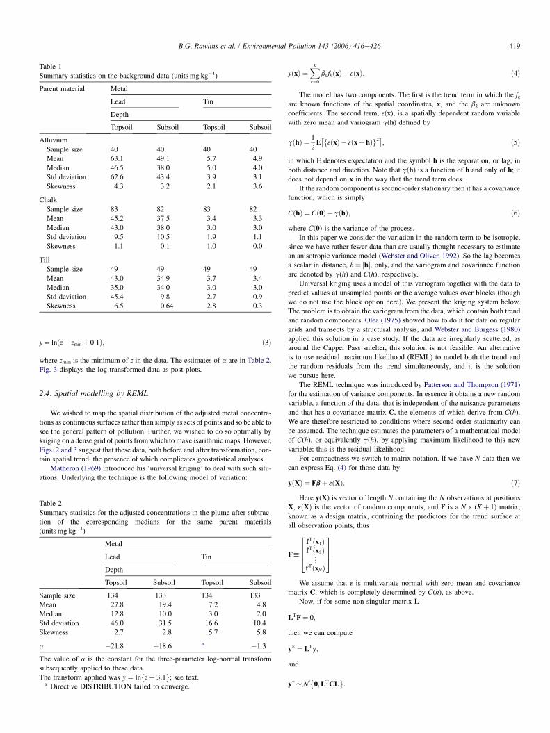
Summary statistics were computed for concentrations of lead and tin in

both topsoil and subsoil of the background data set and also for the subsets

of data identified with the three parent material classes. Table 1 lists the

results. Most of the sets of data were strongly positively skewed (skewness

coefficients> 1). We therefore express the centres of their distributions by

their sample medians rather than their means to avoid giving undue weight

to data in the long upper tails of the distributions.

We then considered the data in the target region separately for each metal,

each depth and for each of the three parent materials. The data for the two

depths were treated separately throughout the subsequent geostatistical analy-

sis. For each set we subtracted the median of the background data and recom-

puted summaries of the residuals, to which we subsequently refer as the

adjusted concentrations in the soil. Although we cannot know the original

values, we have made a pragmatic assumption that the medians of the back-

ground data would be the most reasonable measures of metal concentrations

in the soil in the region before the smelter began operation.

The results are listed in Table 2, and their quintiles are displayed as post-

plots in Fig. 2. All the variables still have strongly skewed distributions, and to

stabilize their variances we transformed them to logarithms after fitting three-

parameter lognormal curves to their frequency distributions using the distribu-

tion directive in GenStat (Payne et al., 2003). The probability density function

for a variable z with such a distribution is given by

f ðzÞ ¼ 1

sðz� aÞffiffiffiffiffiffi2pp exp

�� 1

2s2flnðz� aÞ � mg2

�; ð1Þ

of which the three parameters are the mean, m, the standard deviation, s, and

a shift, a. The transformed variable is

y¼ lnðz� aÞ with ywNðm;sÞ: ð2Þ

The directive DISTRIBUTION did not converge for the data on tin, so

these were transformed by

419B.G. Rawlins et al. / Environmental Pollution 143 (2006) 416e426

y¼ lnðz� zmin þ 0:1Þ; ð3Þ

where zmin is the minimum of z in the data. The estimates of a are in Table 2.

Fig. 3 displays the log-transformed data as post-plots.

2.4. Spatial modelling by REML

We wished to map the spatial distribution of the adjusted metal concentra-

tions as continuous surfaces rather than simply as sets of points and so be able to

see the general pattern of pollution. Further, we wished to do so optimally by

kriging on a dense grid of points from which to make isarithmic maps. However,

Figs. 2 and 3 suggest that these data, both before and after transformation, con-

tain spatial trend, the presence of which complicates geostatistical analyses.

Matheron (1969) introduced his ‘universal kriging’ to deal with such situ-

ations. Underlying the technique is the following model of variation:

Table 1

Summary statistics on the background data (units mg kg�1)

Parent material Metal

Lead Tin

Depth

Topsoil Subsoil Topsoil Subsoil

Alluvium

Sample size 40 40 40 40

Mean 63.1 49.1 5.7 4.9

Median 46.5 38.0 5.0 4.0

Std deviation 62.6 43.4 3.9 3.1

Skewness 4.3 3.2 2.1 3.6

Chalk

Sample size 83 82 83 82

Mean 45.2 37.5 3.4 3.3

Median 43.0 38.0 3.0 3.0

Std deviation 9.5 10.5 1.9 1.1

Skewness 1.1 0.1 1.0 0.0

Till

Sample size 49 49 49 49

Mean 43.0 34.9 3.7 3.4

Median 35.0 34.0 3.0 3.0

Std deviation 45.4 9.8 2.7 0.9

Skewness 6.5 0.64 2.8 0.3

Table 2

Summary statistics for the adjusted concentrations in the plume after subtrac-

tion of the corresponding medians for the same parent materials

(units mg kg�1)

Metal

Lead Tin

Depth

Topsoil Subsoil Topsoil Subsoil

Sample size 134 133 134 133

Mean 27.8 19.4 7.2 4.8

Median 12.8 10.0 3.0 2.0

Std deviation 46.0 31.5 16.6 10.4

Skewness 2.7 2.8 5.7 5.8

a �21.8 �18.6 a �1.3

The value of a is the constant for the three-parameter log-normal transform

subsequently applied to these data.

The transform applied was y ¼ lnfzþ 3:1g; see text.a Directive DISTRIBUTION failed to converge.

yðxÞ ¼XK

k¼0

bk fkðxÞ þ 3ðxÞ: ð4Þ

The model has two components. The first is the trend term in which the fkare known functions of the spatial coordinates, x, and the bk are unknown

coefficients. The second term, 3(x), is a spatially dependent random variable

with zero mean and variogram g(h) defined by

gðhÞ ¼ 1

2E�f3ðxÞ � 3ðxþ hÞg2�; ð5Þ

in which E denotes expectation and the symbol h is the separation, or lag, in

both distance and direction. Note that g(h) is a function of h and only of h; it

does not depend on x in the way that the trend term does.

If the random component is second-order stationary then it has a covariance

function, which is simply

CðhÞ ¼ Cð0Þ �gðhÞ; ð6Þ

where C(0) is the variance of the process.

In this paper we consider the variation in the random term to be isotropic,

since we have rather fewer data than are usually thought necessary to estimate

an anisotropic variance model (Webster and Oliver, 1992). So the lag becomes

a scalar in distance, h¼ jhj, only, and the variogram and covariance function

are denoted by g(h) and C(h), respectively.

Universal kriging uses a model of this variogram together with the data to

predict values at unsampled points or the average values over blocks (though

we do not use the block option here). We present the kriging system below.

The problem is to obtain the variogram from the data, which contain both trend

and random components. Olea (1975) showed how to do it for data on regular

grids and transects by a structural analysis, and Webster and Burgess (1980)

applied this solution in a case study. If the data are irregularly scattered, as

around the Capper Pass smelter, this solution is not feasible. An alternative

is to use residual maximum likelihood (REML) to model both the trend and

the random residuals from the trend simultaneously, and it is the solution

we pursue here.

The REML technique was introduced by Patterson and Thompson (1971)

for the estimation of variance components. In essence it obtains a new random

variable, a function of the data, that is independent of the nuisance parameters

and that has a covariance matrix C, the elements of which derive from C(h).

We are therefore restricted to conditions where second-order stationarity can

be assumed. The technique estimates the parameters of a mathematical model

of C(h), or equivalently g(h), by applying maximum likelihood to this new

variable; this is the residual likelihood.

For compactness we switch to matrix notation. If we have N data then we

can express Eq. (4) for those data by

yðXÞ ¼ Fbþ 3ðXÞ: ð7Þ

Here y(X) is vector of length N containing the N observations at positions

X, 3ðXÞ is the vector of random components, and F is a N� (Kþ 1) matrix,

known as a design matrix, containing the predictors for the trend surface at

all observation points, thus

Fh

2664fTðx1ÞfTðx2Þ

«fTðxNÞ

3775:We assume that 3 is multivariate normal with zero mean and covariance

matrix C, which is completely determined by C(h), as above.

Now, if for some non-singular matrix L

LTF¼ 0;

then we can compute

y� ¼ LTy;

and

y�wN�

0;LTCL�:

420 B.G. Rawlins et al. / Environmental Pollution 143 (2006) 416e426

492000 496000 500000 504000 508000

426000

428000

430000

432000

434000

436000

438000

440000

442000

444000

27 to 4141 to 4949 to 5858 to 7979 to 293

a)

492000 496000 500000 504000 508000

426000

428000

430000

432000

434000

436000

438000

440000

442000

444000 b)

24 to 3636 to 4343 to 5252 to 6868 to 236

492000 496000 500000 504000 508000

426000

428000

430000

432000

434000

436000

438000

440000

442000

444000 c)

2 to 55 to 66 to 99 to 1414 to 147

492000 496000 500000 504000 508000

426000

428000

430000

432000

434000

436000

438000

440000

442000

444000

2 to 44 to 55 to 66 to 99 to 95

d)

Fig. 2. Quintiles of the adjusted metal concentrations (in mg kg�1) within the plume (after subtraction of the sample medians for the corresponding parent material

type in the background data set: (a) Pb in surface soil, (b) Pb in deeper soil, (c) Sn in surface soil and (d) Sn in deeper soil.

For the general linear model, as used here, the log residual likelihood is

(Stuart et al., 1999)

l�fb;b¼ constant� 1

2lnjCj � 1

2lnFTC�1F

� 1

2yTC�1ðI�QÞy; ð8Þ

where

QhF�FTC�1F

�1FTC�1: ð9Þ

In practice we have to enter values into the covariance matrix, C; these are

obtained from a mathematical model of the covariance function, C(h). The pa-

rameters of this covariance function are also parameters of the variogram un-

der second-order stationarity, as expressed in Eq. (6), but it must be

remembered that the covariance function does not exist in all circumstances

when the variogram does. In this paper we use the variogram in our discussion

of spatial variation and estimation, with the implicit assumption of second-or-

der stationarity. In order that we may determine terms of C we must model

C(h), or equivalently the variogram, g(h), with some continuous function of

the lag such that the covariance matrix is necessarily positive definite. There

421B.G. Rawlins et al. / Environmental Pollution 143 (2006) 416e426

492000 496000 500000 504000 508000

426000

428000

430000

432000

434000

436000

438000

440000

442000

444000

-1.1 to 0.00.0 to 1.11.1 to 2.32.3 to 3.43.4 to 4.5

d)

492000 496000 500000 504000 508000

426000

428000

430000

432000

434000

436000

438000

440000

442000

444000

1.2 to 2.12.1 to 3.03.0 to 3.93.9 to 4.74.7 to 5.6

a)

492000 496000 500000 504000 508000

426000

428000

430000

432000

434000

436000

438000

440000

442000

444000

1.5 to 2.32.3 to 3.13.1 to 3.83.8 to 4.64.6 to 5.4

b)

492000 496000 500000 504000 508000

426000

428000

430000

432000

434000

436000

438000

440000

442000

444000

-2.3 to -0.8-0.8 to 0.60.6 to 2.12.1 to 3.53.5 to 5.0

c)

Fig. 3. Log-transformed values (mg kg�1) of the adjusted metal concentrations to the north-east of the smelter ( ): (a) Pb in surface soil, (b) Pb in deeper soil, (c)

Sn in surface soil and (d) Sn in deeper soil. The hachuring is on the side of the smaller values for each contour.

are rather few simple functions that guarantee this condition (see Webster and

Oliver, 2001). The two we have used in this case study are the popular spher-

ical and exponential; their definitions are as follows.

2.4.1. Spherical

gðhÞ ¼ c

�3h

2a� 1

2

�h

a

3�for 0 � h < a

¼ c for h � a: ð10Þ

Here c is the a priori variance of the process and is the upper bound of the

function, its ‘sill’; and a is a distance parameter, the range, which is finite. The

random variables 3(x) and 3(xþ h) are statistically uncorrelated with one an-

other if h� a.

2.4.2. Exponential

gðhÞ ¼ c

�1� exp

��h

r

�: ð11Þ

The exponential function also has a sill, c, which it approaches asymptot-

ically; it does not have a finite range, but an effective range is often taken as

a0 ¼ 3r where it reaches approximately 95% of its sill value.

422 B.G. Rawlins et al. / Environmental Pollution 143 (2006) 416e426

Almost always we must add to such a model a spatially uncorrelated ‘nug-

get’ variance, which we denote c0. So, the complete formula for the spherical

variogram, for example, is

gðhÞ ¼ c0 þ c1

�3h

2a� 1

2

�h

a

3�for 0< h < a

¼ c0 þ c1 for h� a

¼ 0 for h¼ 0: ð12Þ

There are other functions that describe the variogram. Note that only func-

tions for second-order stationary random variables (i.e. bounded variogram

functions) are compatible with the existence of the covariance function. These

simple functions describing the spatial dependence in 3(x) are thus completely

defined by their form, spherical or exponential, and the three parameters,

f¼ ½c0;c1;a�:

To proceed to the kriging we require estimates of these parameters, and we

obtain them for a given type of model by REML. The REML estimates of the

variance parameters are those that maximize the residual likelihood condi-

tional on the data. These are found numerically. The average information

(AI) algorithm of Gilmour et al. (1995) is efficient. It is not suitable for esti-

mating the parameters of spherical model, however, because these do not have

a smooth likelihood function, and so the gradient method used in the AI algo-

rithm can stick at local optima. Lark and Cullis (2004) used simulated anneal-

ing to find the REML estimates of spherical model parameters, and they

discovered that these could be better than those from the AI algorithm; so

this is the method that we have used here.

For each log-transformed variable we estimated the variance parameters

for linear and quadratic trend surfaces after first rescaling the coordinates

from metres to kilometres and adjusting them to a local origin for numerical

stability. We then obtained the REML estimates of the variance parameters

by simulated annealing. We did this for both spherical and exponential models

of the variogram, and finally chose the model for which the maximized resid-

ual likelihood was largest.

Universal kriging does not require the actual trend model to be computed

separately because the trend is implicit in the kriging system. We were not

obliged to estimate the trend parameters b. Nevertheless, we did so; we

computed the estimates and their standard errors by generalized least-squares

so that we could see whether particular components of the two trend models

were likely to be useful, and so select a model to use in the kriging. The gen-

eralized least-squares estimate of b is

b¼�FTC�1F

�1FTC�1y: ð13Þ

Two comments on the assumptions of the REML analysis are worth mak-

ing. First, we noted above that 3 is assumed to be a realization of a multivariate

normal process. Since we can only have one observation of 3 (one observation

at each sample site) this assumption is unverifiable. It is supported (although

not ensured) if the histogram of the data appears approximately normal, per-

haps after transformation. However, Kitanidis (1985) showed that likeli-

hood-based estimates of spatial variance parameters were robust to

departures from normality in simulations; and Pardo-Iguzquiza (1998) showed

that, given our ignorance of the actual underlying multivariate distribution, the

assumption of normality may be justified by an entropy criterion.

Second, we assume the existence of a covariance matrix for 3. This

requires that the random process be second-order stationarity, a stronger

requirement than the intrinsic hypothesis, which is all that is necessary for

the existence of the variogram. We are therefore limited to bounded vario-

grams, such as the spherical (in which the sill value is the maximum variance)

and the exponential (which is asymptotically bounded by the sill variance).

2.5. Lognormal universal kriging

We transformed the original concentrations to approximately normally dis-

tributed variables, y, as described above. We then predicted values of the y at

the nodes of a fine grid by punctual universal kriging (UK) based on all the

topsoil and deeper soil data separately. The UK estimate of a variable is the

empirical best linear unbiased predictor (E-BLUP) conditional on the selected

trend model (Stein, 1999), and denoted ‘empirical’ because it is also condi-

tional on our model for the variogram derived from the data.

For each target position x0 the prediction is a linear combination of the N

values of y:

eYðx0Þ ¼XN

i¼1

liyðxiÞ: ð14Þ

Its expectation is

EheYðx0Þ

i¼XK

k¼0

XN

i¼1

bkli fkðxiÞ; ð15Þ

and the prediction is unbiased if

XN

i¼1

li fkðxÞ ¼ fkðx0Þ for all k ¼ 1;2;.;K: ð16Þ

Subject to this condition the weights li are chosen to minimize the

expected mean squared error of the prediction, the UK variance sUK2 , by solu-

tion of the following system of equations:

XN

i¼1

lig�xi � xj

þj0 þ

XK

k¼1

jk fk

�xj

¼ g

�x0 � xj

for all j ¼ 1;2;.;N;

XN

i¼1

li¼ 1;

XN

i¼1

lifkðxÞ ¼ fkðx0Þ for all k ¼ 1;2;.;K: ð17Þ

This is the universal kriging system in which the g(xi� xj) are the

semivariances of 3(x) between the data points xi and xj, and g(x0� xj)

are the semivariances between the target point, x0 and the data points.

The quantities jk, k¼ 0,1,2,.,K, are Lagrange multipliers introduced for

the minimization of the variance subject to the unbiasedness constraints.

It is a set of linear equations, which can be succinctly written in matrix

notation as

Al¼ u: ð18Þ

Matrix A is

A¼

26666666666664

gðx1�x1Þ gðx1�x2Þ . gðx1�xNÞ 1 f1ðx1Þ f2ðx1Þ . fKðx1Þgðx2�x1Þ gðx2�x2Þ . gðx2�xNÞ 1 f1ðx2Þ f2ðx2Þ . fKðx2Þ

« « . « « « « . «gðxN�x1Þ gðxN �x2Þ . gðxN�xNÞ 1 f1ðxNÞ f2ðxNÞ . fKðxNÞ

1 1 . 1 0 0 0 . 0f1ðxÞ1 f1ðx2Þ . f1ðxNÞ 0 0 0 . 0f2ðxÞ1 f2ðx2Þ . f2ðxNÞ 0 0 0 . 0

« « . « « « « . «fKðxÞ1 fKðx2Þ . fKðxNÞ 0 0 0 . 0

37777777777775and l and u are

l¼

26666666666664

l1

l2

«lN

j0

j1

j2

«jK

37777777777775and u¼

26666666666664

gðx1 � x0Þgðx2 � x0Þ

«gðxN � x0Þ

1f1ðx0Þf2ðx0Þ

«fKðx0Þ

37777777777775:

We solve the kriging equation by

l¼ A�1u; ð19Þ

to obtain the kriging weights, li, l2,., which we then insert into Eq. (14) to

give our predictions. The kriging variance is given by

s2UK ¼ uTl: ð20Þ

423B.G. Rawlins et al. / Environmental Pollution 143 (2006) 416e426

Universal kriging returns the E-BLUP for the normal variable Y(x); but we

require estimates on the scale of the original data z(x). As with any estimate

derived from log-transformed data, we cannot simply back transform the esti-

mates on the logarithmic scale; we must also correct for bias. Cressie (2004)

has shown that the UK estimate of a lognormal variable eZ0ðx0Þ, based on the

UK estimate eYðx0Þof the corresponding Y, is

eZ0ðx0Þ ¼ exp

(eYðx0Þ þ1

2s2

UK �j0 �XK

i¼1

ji fiðx0Þ): ð21Þ

We therefore back-transformed our kriged estimates in this way.

We kriged the log-transformed variables at the nodes of a regular grid with

interval 500 m over the region. We specified the predictor variables selected

after the trend analysis of the data using REML, and used the variogram model

estimated by REML. We used all observations for every kriging system be-

cause we wanted the trend model at all target sites to be the same as the overall

trend model to which our variogram refers. We then used Eq. (21) to back-

transform the estimates to the original scale, and corrected for the shift con-

stant, a or zmin, in the log-transformation. The final predictions of adjusted

metal were then ‘contoured’ to produce the isarithmic maps displayed in

Fig. 4.

3. Results and their interpretation

3.1. Trend and variogram models based on REML

We examined the parameter estimates b for the quadraticand linear trend, for both metals and both depths, with which-ever of the spherical and exponential variogram models max-imized the residual likelihood. We noted that in all cases theparameters for the quadratic terms, and the linear term inthe eastings were small relative to their standard errors (a tratio smaller than 1.96). The linear coefficient for the northingwas always large (except for topsoil tin for which it was largerthan any other coefficient, but with a t ratio still smaller than1.96). For this reason we fitted a simple trend surface linear inthe northing for all variables.

Since the trend appears to be limited to one direction, anexperimental variogram for the error variable 3(x) couldhave been obtained by the usual method of moments estimator

492000 496000 500000 504000 508000

426000

428000

430000

432000

434000

436000

438000

440000

442000

444000

492000 496000 500000 504000 508000

426000

428000

430000

432000

434000

436000

438000

440000

442000

444000

a)

b)

492000 496000 500000 504000 508000

426000

428000

430000

432000

434000

436000

438000

440000

442000

444000

492000 496000 500000 504000 508000

426000

428000

430000

432000

434000

436000

438000

440000

442000

444000

c)

d)

Fig. 4. Contour maps of adjusted metal concentrations (in mg kg�1) around the smelter ( ) for (a) Pb in surface soil, (b) Pb in deeper soil, (c) Sn in surface soil and

(d) Sn in deeper soil. The hachuring is on the side of the smaller values for each contour.

424 B.G. Rawlins et al. / Environmental Pollution 143 (2006) 416e426

applied only to comparisons between pairs of points separatedby a lag vector perpendicular to this trend. A model, such asthe exponential or spherical could then have been fitted tothis and used for kriging. This approach, which is often advo-cated for geostatistical analysis of data with trend, might bepreferred to REML because it is simpler. However, we con-cluded that this particular trend model is appropriate from in-ferences about the parameters of different models that areminimum variance estimates only because we have estimatedthem with REML. Further, the fact that we have used REMLmeans that all paired comparisons between observations con-tribute to our estimate of the variance parameters, not justa subset which might be small when the sampling sites areirregularly scattered.

Table 3 lists the parameters of the fitted models. Note that,apart from subsoil tin, the range of spatial dependence is large,and that for topsoil tin the variogram is still far from its boundat lag distances within the confines of the region. However, theeffective range is not smaller for more complex trend models,and the fact that the coefficients for higher-order trend compo-nents are small suggests that the long-range variation, afterremoval of the linear trend on northings, can be treated asrandom.

3.2. Geochemical maps of adjusted metal concentration

There is a striking difference between the map of adjustedPb in the topsoil (Fig. 4a) and that in the subsoil (Fig. 4b): theformer has steep gradients around the site of the smelter,whereas the latter does not. In addition, there are two excep-tionally large Pb concentrations (293 and 194 mg kg�1) sur-rounded by a series of closely spaced contours to the east onthe topsoil map with nothing comparable on the map of thesubsoil. The two locations are on the urban fringe of Hull,and the large concentrations there might be from a sourceother than the smelter. Otherwise, the two maps are similarin showing towards the north-east end of the plume (504 kmeasting and 438 km northing) concentrations of 60 to80 mg kg�1 greater than those of the backgrounds of the par-ent materials. There are also unusually large concentrations ofSn in the topsoil in the same part of the region (Fig. 4c). Ifthese larger concentrations of Pb and Sn are the result of de-position of particles emitted from the smelter then this patternis contrary to observations that metal deposition diminishes

Table 3

Models fitted to log-transformed, adjusted metal concentrations

Metal Depth b0 b1 t Ratioa Model c0 c1 a/km r/km

Lead Topsoil 4.53 �0.098 2.24 Spherical 0.22 0.46 18.0

Subsoil 4.01 �0.066 1.95 Spherical 0.2 0.36 18.9

Tin Topsoil 3.22 �0.151 2.55 Exponential 0.33 1.30 21.3

Subsoil 2.07 �0.084 2.23 Exponential 0.32 0.41 5.6

The parameters b0 and b1 are for the trend from south to north (and coordi-

nates in km), and c0, c1 and a and r (in km) are those of the variogram models

of the random components.a For null hypothesis that b1¼ 0.

rapidly with increasing distance (De Caritat et al., 1997). Ondays with strong south-westerly winds, particulate depositionmight have been enhanced in this part of the region whichforms the leeward slope of the northesouth trending YorkshireWolds (diminishing rapidly from a maximum elevation of60 m). Alternatively, the larger concentrations might simplybe due to natural variation in the geochemistry of the parentmaterials. One might resolve this uncertainty by further inves-tigations based on differences in the Pb isotope composition ofthe smelter emissions and native Pb in the soil.

3.3. Estimates of excess metal in the soil

We wanted to estimate the excess quantities of Pb and Sn inthe soil across the 286 km2 of the plume, based on our krigedestimates of adjusted metal concentration. We assumed thatthe topsoil and deeper soil samples would provide reasonableestimates of the concentration across their depth ranges (0e15 cm and 25e40 cm, respectively). We also assumed thatthe average of the concentrations at these two depths wouldbe a reasonable estimate for the soil in the depth interval(15e25 cm), subsequently referred to as the intermediatedepth.

We selected the final estimates of adjusted metal concentra-tions from the nodes of our 500-m grid at each of the threedepths. We then averaged these to provide an estimate of theaverage adjusted metal content of the soil across the plume.We converted the adjusted metal concentrations into totalquantities of metal in the soil (at each of the three depths).Here we made assumptions concerning the proportions ofstones in the soil and its bulk density. The dominant soil typesin the region, as judged from the scheme of soil classificationadopted in England and Wales (Avery, 1990), are ‘fine loamysoils’ and ‘well drained calcareous fine silty soils’. We haveassumed a stone content of 10% e the centre of the classtermed slightly stony (Avery, 1990) e and a typical soilbulk density of 1.35 g cm�3 (Soil Survey of England andWales, 1977) uniform down to 45 cm. We then aggregatedthe total amount of adjusted metal for each node within theplume at each of the depths for both metals.

The aggregated adjusted metal will overestimate the excessmetal, as defined above, since it is based on the difference be-tween the observed metal concentration and the median back-ground concentration for the parent material. For this reasonwe took the difference between the mean and median back-ground concentrations (Table 1) and from these computeda correction to the aggregated metal concentration over theplume. We calculated the mass of soil over the area of eachparent material in the plume, till (108 km2), chalk (106 km2)and alluvium (74 km2), making the same assumptions aboutbulk density and stoniness that we describe above. We multi-plied this mass by the difference between the mean and me-dian concentration in the corresponding background, andsummed these results to obtain an overall correction. The cor-rections were then subtracted from the aggregated adjustedmetal to provide an estimate of excess metal. For the interme-diate depth we used the average of the corrections for the

425B.G. Rawlins et al. / Environmental Pollution 143 (2006) 416e426

topsoil and subsoil. Over the area of the plume, we estimatedexcess amounts of Pb to be 1174, 633 and 723 t for the top,intermediate and deeper soil, respectively. The correspondingamounts of excess Sn are 424, 208 and 199 t. Given that ourestimates are based on several assumptions, we express the to-tal excess metal estimates to two significant figures. Hence, weestimate that the total excess Pb is approximately 2500 t, andtotal excess Sn is 830 t. The downward transfer of aerially de-posited particles is likely to have been enhanced by ploughing(plough depths typically 20e30 cm) as arable agriculture isthe dominant land use in the region. Our estimates cannot ac-count for any excess metal transported below 40 cm.

In addition to Pb derived from the smelter, there are diffusesources in the locality (particularly Pb from vehicle exhausts)which could in part contribute to the estimate of excess metal.However, the background sample subset would also have beensubject to diffuse, aerial deposition of Pb, and therefore part ofits impact is likely to have been cancelled out. Notwithstand-ing this, we did compare the range of diffuse inputs based ondata for aerial deposition of Pb to agricultural soils across En-gland from major sources between 1995 and 1998 (Nicholsonet al., 2003) with our estimates of excess Pb. The minimumand maximum rates are equivalent to 0.54 and 4.0 t Pb peryear across the plume. Even at the maximum rate of Pb depo-sition reported by Nicholson et al., the total over 20 years isunlikely to exceed 80 t over the area of the plume.

4. Discussion

We believe that, in the absence of other significant sourcesof Sn in the local environment, the vast majority of excess Pband Sn in the soil across the region came from the Capper Passsmelter as fallout of airborne particulates. Unpublished databased on scanning electron microscope analyses of bark sam-ples from present-day trees and attic dusts provide further ev-idence to support this conclusion. A previous analysis ofmalignancies among both children and adults in north Hum-berside showed increased risks close to the smelter (Alexanderet al., 1984). Data on the magnitude and distribution of histor-ical metal deposition related to the former operation of thesmelter could aid subsequent epidemiological studies.

Acknowledgements

We thank all the staff of the British Geological Survey andvolunteers involved in the collection and analysis of soil sam-ples in the G-BASE project, and an anonymous reviewer forhelpful comments on an earlier draft of the script. This paperis published with the permission of the Director of the BritishGeological Survey (Natural Environment Research Council).R.M. Lark’s contribution was supported by Rothamsted Re-search’s core grant from the Biotechnology and BiologicalSciences Research Council.

References

Alexander, F., McKinney, P.A., Cartwright, R.A., 1984. The pattern of child-

hood and related adult malignancies near Kingston-upon-Hull. Journal of

Public Health Medicine 13, 96e100.

Avery, B.W., 1990. Soils of the British Isles. CAB International, Wallingford.

British Geological Survey, 1983a. York Sheet 63: Solid and Drift. Ordnance

Survey for the Institute of Geological Sciences, Southampton.

British Geological Survey, 1983b. Kingston Upon Hull Sheet 80: Solid and

Drift. Ordnance Survey for the Institute of Geological Sciences,

Southampton.

British Geological Survey, 1993. Great Driffield Sheet 64: Solid and Drift.

British Geological Survey, Keyworth.

British Geological Survey, 1995. Beverley Sheet 72: Solid and Drift. British

Geological Survey, Keyworth.

British Geological Survey, 2000. Regional Geochemistry of Wales and Part of

West-central England e Stream Sediment and Soil. British Geological

Survey, Keyworth.

Colgan, A., Hankard, P.K., Spurgeon, D.J., Svendsen, C., Wadsworth, R.A.,

Weeks, J.M., 2003. Closing the loop: a spatial analysis to link observed

environmental damage to predicted heavy metal emissions. Environmental

Toxicology and Chemistry 22, 970e976.

Cressie, N., 2004. Block Kriging for Lognormal Spatial Processes. Technical

Report No 739. Department of Statistics, Ohio State University, Columbus,

OH.

De Caritat, P., Reimann, C., Chekushin, V., Bogatyrev, I., Niskavarra, H.,

Braun, J., 1997. Mass balance between emission and deposition of airborne

contaminants. Environmental Science and Technology 31, 2966e2972.

Department of the Environment, 1992. The UK Environment. Her Majesty’s

Stationery Office, London.

Gilmour, A.R., Thompson, R., Cullis, B.R., 1995. Average information

REML: an efficient algorithm for variance parameter estimation in linear

mixed models. Biometrics 51, 1440e1450.

Govindaraju, K., 1994. Compilation of working values and sample description

for 383 geostandards. Geostandards Newsletter 18, 1e158.

Kitanidis, P.K., 1985. Minimum-variance unbiased quadratic estimation of

covariances of regionalized variables. Journal of the International

Association of Mathematical Geology 17, 195e208.

Lark, R.M., Cullis, B.R., 2004. Model-based analysis using REML for infer-

ence from systematically sampled data on soil. European Journal of Soil

Science 55, 799e813.

Litten, J.A., Strachan, A.M., 1995. Aspects of the closure of Capper Pass and

Son. Minerals Industry International (May), 28e34.

Matheron, G., 1969. Le krigeage universel. Cahiers du Centre de Morphologie

Mathematique. Ecole des Mines de Paris, Fontainebleau.

McMartin, I., Henderson, P.J., Nielsen, E., 1999. Impact of a base metal

smelter on the geochemistry of soils of the Flin Flon region, Manitoba

and Saskatchewan. Canadian Journal of Earth Sciences 36, 141e160.

Nahmani, J., Lavelle, P., Lapied, E., van Oort, F., 2003. Effects of heavy metal

soil pollution on earthworm communities in the north of France. Pedobio-

logia 47, 663e669.

Nicholson, F.A., Smith, S.R., Alloway, B.J., Carlton-Smith, C., Chambers, B.,

2003. An inventory of heavy metals inputs to agricultural soils in England

and Wales. Science of the Total Environment 311, 205e219.

Olea, R.A., 1975. Optimum mapping techniques using regionalized variable

theory. In: Series on Spatial Analysis No 2. Kansas Geological Survey,

Lawrence, Kansas.

Pardo-Iguzquiza, E., 1998. Maximum likelihood estimation of spatial covari-

ance parameters. Mathematical Geology 30, 95e108.

Patterson, D.D., Thompson, R., 1971. Recovery of inter-block information

when block sizes are unequal. Biometrika 58, 545e554.

Payne, R., Murray, D., Harding, S., Baird, D., Soutar, D., Lane, P., 2003.

GenStat for Windows. VSN International, Hemel Hempstead.

Roels, H.A., Buchet, J.P., Lauwerys, R.R., Bruaux, P., Claeys-Thoreau, F.,

Lafontaine, A., Verduyn, G., 1980. Exposure to lead by the oral and the

pulmonary routes of children living in the vicinity of a primary lead

smelter. Environmental Research 22, 81e94.

426 B.G. Rawlins et al. / Environmental Pollution 143 (2006) 416e426

Soil Survey of England and Wales, 1977. Water Retention, Porosity and

Density of Field Soils. Technical Monograph No 9. Lawes Agricultural

Trust, Harpenden.

Stein, M.L., 1999. Interpolation of Spatial Data: Some Theory for Kriging.

Springer, New York.

Sterckeman, T., Douay, F., Proix, N., Fourrier, H., Perdrix, E., 2002. Assess-

ment of the contamination of cultivated soils by eighteen trace elements

around smelters in the North of France. Water, Air and Soil Pollution

2002, 173e194.

Stuart, A., Ord, J.K., Arnold, S., 1999. Kendall’s advanced theory of statistics. In:

Classical Inference and the Linear Model, sixth ed., vol. 2A. Arnold, London.

Webster, R., Burgess, T.M., 1980. Optimal interpolation and isarithmic map-

ping of soil properties. III. Changing drift and universal kriging. Journal

of Soil Science 31, 505e524.

Webster, R., Oliver, M.A., 1992. Sample adequately to estimate variograms of

soil properties. Journal of Soil Science 43, 177e192.

Webster, R., Oliver, M.A., 2001. Geostatistics for Environmental Scientists.

John Wiley and Sons, Chichester.