The University of Edinburgh School of Engineering

BRE Centre for Fire Safety Engineering

Academic Year 2018-19

DESIGN OF VENTILATION AND SUPPRESSION SYSTEMS FOR FIRES IN ROAD TUNNELS

James Crum Promoter: Dr Ricky Carvel

Master thesis submitted in the Erasmus+ Study Programme International Master of Science in Fire Safety Engineering

Disclaimer This thesis is submitted in partial fulfilment of the requirements for the degree of The International Master of Science in Fire Safety Engineering (IMFSE). This thesis has never been submitted for any degree or examination to any other University/programme. The author declares that this thesis is original work except where stated. This declaration constitutes an assertion that full and accurate references and citations have been included for all material, directly included and indirectly contributing to the thesis. The author gives permission to make this master thesis available for consultation and to copy parts of this master thesis for personal use. In the case of any other use, the limitations of the copyright have to be respected, in particular with regard to the obligation to state expressly the source when quoting results from this master thesis. The thesis supervisor must be informed when data or results are used. Word count: Read and approved, James Crum 30 April 2019

ABSTRACT The interaction between water mist systems and ventilation systems in tunnel fires was modelled by creating a MATLAB program to solve a system of equations generated using comprehensive thermodynamic control volume analyses. The program uses input values for relevant variables in order to estimate the number of jet fans required to prevent smoke backlayering in a tunnel fire. The input variables include tunnel dimensions, water mist system characteristics, and fire size. A case study was performed on a 6 x 6 x 600 m tunnel in keeping with previous research. It was found that the use of a water mist system had a mixed impact on the number of fans required to prevent backlayering. At heat release rates lower than approximately 15 MW, it was found that the water mist system increased the number of fans required. The main reason for this was determined to be the resistance caused by accelerating the relatively large mass of water introduced into the tunnel. At heat release rates larger than approximately 15 MW, it was found that the water mist system reduced the number of fans required. This was determined to be due to the ability of the water mist system to reduce the heat release rate and to reduce the downstream temperatures. Several recommendations for future work were made. They mostly concerned collecting more full-scale experimental data in several areas, including: determining the relationship between water mist system characteristics and heat release rate, determining what proportion of water spray evaporates in a tunnel fire, measuring the throttling effect of a fire on longitudinal airflow, and determining the relationship between longitudinal ventilation velocity and water mist systems.

ACKNOWLEDGEMENTS I would like to thank my supervisor Dr Ricky Carvel for his advice, guidance and support throughout the project. The thesis would not have possible without his invaluable contribution. I must also pay tribute to my flatmates, Dheeraj Dilip Karyaparambil and Balša Jovanović. Their thoughtful opinions, technical expertise and motivating words were major factors contributing to this work being completed on time.

Table of Contents NOTATION ............................................................................................................................. 11. INTRODUCTION .............................................................................................................. 2

1.1. Overview ....................................................................................................................... 21.2. Tunnel Fire Dynamics ................................................................................................ 41.3. Heat Release Rates in Tunnels .................................................................................. 51.4. Tunnel Ventilation ...................................................................................................... 7

1.4.1. Ventilation Systems .......................................................................................... 71.4.2. Throttling Effect ................................................................................................ 71.4.3. Tunnel Ventilation Velocity ............................................................................ 8

1.5. Fixed Firefighting Systems ...................................................................................... 121.5.1. Overview .......................................................................................................... 121.5.2. Dynamics of Suppression by Water Sprays ................................................ 13

1.7. Modelling of Tunnel Fires ....................................................................................... 131.8. Problem Statement and Objectives ........................................................................ 14

2. METHODOLOGY ............................................................................................................ 152.1. Overview ..................................................................................................................... 152.2. Algorithm .................................................................................................................... 17

2.2.1. Problem Initialisation .................................................................................... 172.2.2. Heat Release Rate Adjustment ..................................................................... 182.2.3. Control Volume Analyses .............................................................................. 202.2.4. Force Balance ................................................................................................... 30

2.3. Model Validation ....................................................................................................... 312.3.1 Overview ........................................................................................................... 312.3.2. Downstream Temperatures ............................................................................ 312.3.3. Backlayer Prevention ..................................................................................... 36

3. RESULTS AND DISCUSSION ..................................................................................... 383.1. Overview ..................................................................................................................... 383.2. Case Study ................................................................................................................... 38

3.2.1. Ambient Conditions ........................................................................................ 383.2.2. Unsuppressed Fires .......................................................................................... 403.2.3. Suppressed Fires ............................................................................................... 47

4. CONCLUSIONS ............................................................................................................... 53REFERENCES ........................................................................................................................ 54APPENDICES ........................................................................................................................ 58

1

NOTATION

! Area (m2) ! Rate of work (W)

!! Drag coefficient (-) ! Elevation (m)

!! Hydraulic diameter (m)

! Energy (J)

! Friction coefficient (-)

! Force (N)

! Gravity (m/s2)

! Height (m) Greek symbols

ℎ Specific enthalpy (J/kg) ! Thermal diffusivity (m2/s)

!

Heat release rate enhancement due to forced ventilation (-) !!"#$ Convective fraction (-)

!!" Entrance loss coefficient (-) !!"# Radiative fraction (-)

!! Jet fan coefficient (-) ! Density (kg/m3)

!!"##$% Nozzle coefficient (-) !!!,!"" Effective heat of combustion (J/kg)

!!"#$$%& Traffic density (-) ! Heat release rate enhancement due to enclosure effects (-)

!!"# Heat release rate reduction due to water mist system operation (-) ! Kinematic viscosity (m2/s)

! Length (m)

! Mass flow rate (kg/s)

!!"#!! Water density (l/min/m2)

!!"#!!! Water flux density (l/min/m3)

! Molar mass (kg/mol)

! Pressure (Pa)

! Heat release rate (W)

!∗ Dimensionless heat release rate (-)

! Ideal gas constant (J/kg/mol)

! Temperature (K)

! Velocity (m/s)

!∗ Dimensionless velocity (-)

! Width (m)

2

1. INTRODUCTION

1.1. Overview Road tunnels are an essential part of many transport networks around the world. They are used to move people and cargo from place to place in a timely manner. Societies expect these tunnels to have an acceptable level of safety for users, at a reasonable economic cost. The risk of fire in a road tunnel poses a major safety hazard to people and can cause extensive damage requiring a lot of time and money to repair. As such, it is important that designers adequately address the threat of fire. Industry attempts to do this by formulating and implementing fire safety strategies. The main goals of a fire safety strategy in a road tunnel are related to life safety and property protection. According to the Tunnel Study Centre (CETU), the main threats to life caused by fire in a road tunnel are exposure to toxic gases and high temperatures [1]. Reduced visibility due to smoke exacerbates these issues, as it can impair self-evacuation and lead to increased exposure times. The main threat to the tunnel itself is high temperatures, which can cause concrete spalling, damage to the road surface, and destruction of services installed in the tunnel. This leads road tunnel designers to try to minimise the temperature and human exposure to toxicity during fires. There are many possible approaches that can be taken to mitigate the threat posed by fires in tunnels. Given the acceptance and widespread implementation of sprinklers in buildings around the world, it would seem that similar systems could be used effectively in tunnels. However, the World Road Association (PIARC) produced a report in 1999 saying that sprinklers are not useful for saving lives in tunnel fires [2]. This maintained the theme of previous reports by PIARC dating back to at least 1983 [3]. The reasons cited include: the inability to suppress fires inside vehicles, the potential to cause explosions through dispersing petrol or other chemicals, vaporised steam burning tunnel occupants, reduced visibility, and destratification of smoke exposing people to toxic gases. The report discusses longitudinal ventilation systems, where smoke is pushed out one end of the tunnel using jet fans. It also examines transverse and semi-transverse systems, where smoke is extracted through ducts. The report gives more weight to the use of such ventilation systems in fire strategies.

3

However, in 1999 and the years since, there have been many examples of major fires in road tunnels. Carvel and Marlair provided a summary of fatal or otherwise significant fires in tunnels over the last 100 years or so [4]. One of the most well known is the Mont Blanc tunnel fire in 1999, which resulted in 39 deaths and extensive damage to the tunnel. An event of this scale is clearly unacceptable, and a response from the industry was required. Designers have since moved towards the use of fixed fire fighting systems (FFFSs). This is probably partly due to the severity of fires such as the Mont Blanc event, where the heat release rate (HRR) was estimated at approximately 190 MW [4]. Full-scale tunnel fire experiments conducted by Ingason measured HRRs in excess of 200 MW [5]. Fires this large are likely to create untenable conditions for people and cause major damage to the tunnel. Deluge sprinkler systems can help prevent fires growing to these sizes, but they use a lot of water. This results in large water storage, pumping, and drainage costs. Water mist systems (WMSs) have shown some ability to limit the HRR and temperatures in full-scale tunnel fire experiments [6][7]. They also use much less water than deluge systems, which can result in substantial monetary savings. Such systems have recently been installed in major urban road tunnels such as the A86 tunnel near Paris and the M30 Madrid ring road [8]. By installing WMSs in tunnels, designers hope to control the HRR of fires and subsequently limit temperatures, smoke production and flame spread. At present, designers assume a design HRR and then design the ventilation system ignoring the effect of the additional mass of water introduced by WMSs. This additional mass, and the subsequent volume of steam produced, could impact the ability of the ventilation system to control smoke produced by the fire. Longitudinal ventilation systems are often designed to prevent the occurrence of backlayering; a phenomenon where smoke flows upstream of the fire, against the direction of forced ventilation. This gives rise to the question: how does a WMS impact on the ability of a longitudinal ventilation system to prevent backlayering in tunnel fires? Previous work by Looi [9] attempted to answer this question using the software programme Fire Dynamics Simulator [10]. This thesis is a continuation of Looi’s, but will attempt to answer the question using a one-dimensional control volume model implemented numerically in MATLAB [11].

4

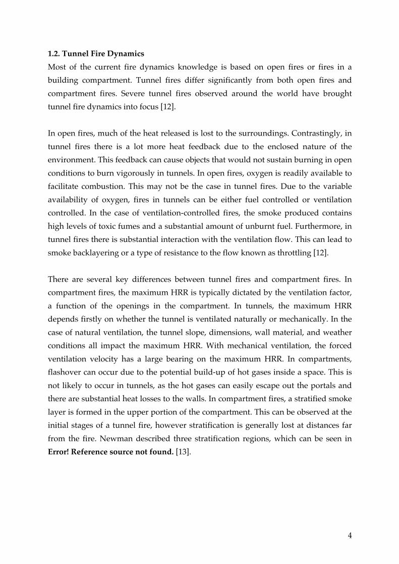
1.2. Tunnel Fire Dynamics Most of the current fire dynamics knowledge is based on open fires or fires in a building compartment. Tunnel fires differ significantly from both open fires and compartment fires. Severe tunnel fires observed around the world have brought tunnel fire dynamics into focus [12]. In open fires, much of the heat released is lost to the surroundings. Contrastingly, in tunnel fires there is a lot more heat feedback due to the enclosed nature of the environment. This feedback can cause objects that would not sustain burning in open conditions to burn vigorously in tunnels. In open fires, oxygen is readily available to facilitate combustion. This may not be the case in tunnel fires. Due to the variable availability of oxygen, fires in tunnels can be either fuel controlled or ventilation controlled. In the case of ventilation-controlled fires, the smoke produced contains high levels of toxic fumes and a substantial amount of unburnt fuel. Furthermore, in tunnel fires there is substantial interaction with the ventilation flow. This can lead to smoke backlayering or a type of resistance to the flow known as throttling [12]. There are several key differences between tunnel fires and compartment fires. In compartment fires, the maximum HRR is typically dictated by the ventilation factor, a function of the openings in the compartment. In tunnels, the maximum HRR depends firstly on whether the tunnel is ventilated naturally or mechanically. In the case of natural ventilation, the tunnel slope, dimensions, wall material, and weather conditions all impact the maximum HRR. With mechanical ventilation, the forced ventilation velocity has a large bearing on the maximum HRR. In compartments, flashover can occur due to the potential build-up of hot gases inside a space. This is not likely to occur in tunnels, as the hot gases can easily escape out the portals and there are substantial heat losses to the walls. In compartment fires, a stratified smoke layer is formed in the upper portion of the compartment. This can be observed at the initial stages of a tunnel fire, however stratification is generally lost at distances far from the fire. Newman described three stratification regions, which can be seen in Error! Reference source not found. [13].

5

Fig. 1. Three stratification regions as described by Newman [13].

The three regions defined by Newman [13] can be described as follows:

• Region I, Fr ≤ 0.9: Obvious stratification. High temperatures at ceiling level, temperatures approximately equal to ambient at ground level. Buoyancy dominated temperature stratification.

• Region II, 0.9 < Fr ≤ 10: No clear stratification, but substantial temperature gradients. Strong interaction between buoyancy forces and the imposed horizontal flow.

• Region III, Fr > 10: Insignificant stratification. Minimal temperature gradients. The Froude number can be calculated using Eq. (1), as follows [12]:

!" = !!"#!

1.5(!!!"# !!"#)!"

(1)

where H is the ceiling height, !!"# is the average gas temperature (K) over the entire

cross-section at a given position, !!!"# = !!"# − !! (the average gas temperature rise

(K) above ambient over the entire cross-section at a given position), and !!"# =!!!"#/!! (m/s) [12].

1.3. Heat Release Rates in Tunnels The HRR in a tunnel fire is dependent on many factors, including the tunnel construction, the type and number of vehicles in the tunnel, and the ventilation conditions [14]. The HRR is a key parameter in the design of safety systems in tunnels. Typically, designers use tabulated peak HRR values from sources such as PIARC [2] or the National Fire Protection Association (NFPA) [15]. Ingason summarised the results of most full-scale tunnel fire experiments performed in the

6

past 25 years, which also provides data that could be used for design purposes. This summary found that the peak HRR ranges from 1.5-11 MW for cars, 25-34 MW for buses, and 13-202 MW for heavy goods vehicles (HGVs) [14]. These experiments were carried out under a range of different circumstances, with important factors such as the ventilation conditions varying between tests. It can be seen that HGVs result in the highest HRRs. As such, they are commonly considered to be the highest risk when designing tunnel ventilation systems. Carvel et al. proposed the following equations to predict the relationship between the HRR in a naturally ventilated tunnel and the HRR in open, ambient conditions [16][17][18]:

!!"##$% = !!!"#$ (2)

! = 24 !!!!

!+ 1 (3)

where ! is the enclosure enhancement factor, !! is the width of the fire object, !! is

the width of the tunnel. This equation is only valid for !! !! values up to 0.5. Carvel and Beard proposed the following equation quantifying the HRR enhancing effect of forced ventilation in HGV fires [19]:

!!"#$%&'$"( = !!!"##$% (4)

where ! is the forced ventilation enhancement factor, which depends on the forced

ventilation velocity. A series of curves were proposed to quantify the value of ! in

the growth phase and for fully involved HGV fires. The value of ! was presented for various percentile values and the expected value. Curves were presented for both one-lane and two-lane tunnels. These curves show that forced ventilation can result in substantially higher HRRs than would otherwise be observed. For example, the

expected ! value is approximately 4 for an HGV fire in the growth phase with a forced ventilation velocity of 3 m/s in a one-lane tunnel.

7

1.4. Tunnel Ventilation

1.4.1. Ventilation Systems There are two main types of ventilation systems used in tunnels: longitudinal and transverse. A longitudinal system moves air along the length of the tunnel. A transverse system moves air both along the length of the tunnel and transverse to the tunnel, depending on the type of transverse system [20]. Ventilation systems can also be divided into naturally and mechanically driven systems. Naturally ventilated systems predominantly rely on meteorological conditions and the longitudinal flow generated by moving vehicles (known as the piston effect). The main meteorological effects driving natural ventilation are wind, elevation differences, and temperature differences. However, these effects are generally not reliable enough to base a fire strategy on. As such, a mechanical system is often required [20]. There are three main types of mechanically powered longitudinal systems: injection, jet fans, and push-pull systems. Injection systems use a fan to push air through a nozzle at ceiling level, which induces a flow through the tunnel. Jet fan systems use a series of jet fans along the length of the tunnel, which accelerate the air and create a longitudinal flow in the tunnel. Push-pull systems use reversible fans located in ventilations shafts at ceiling level; fans upstream of the fire are set to supply mode while downstream fans are set to extract mode [20]. There are three main types of mechanically powered transverse systems: fully transverse, semi-transverse – exhaust, and semi-transverse – supply. A fully transverse system uses a full-length supply duct and a full-length exhaust duct. Semi-transverse – exhaust systems employ a full-length exhaust duct but no supply duct. Semi-transverse – supply systems are the opposite; they have a full-length supply duct but no exhaust duct [20].

1.4.2. Throttling Effect The throttling effect of a fire in a tunnel causes increased resistance to longitudinal flow. This is partially due to the buoyancy of combustion products generating aerodynamic resistance [12]. Lee et al. experimentally measured this phenomenon in 1979. It was found that the flow resistance in the fire zone increased by a factor of 6,

8

and a factor of 1.5 in the upstream and downstream regions due to the throttling effect [21]. Colella et al. numerically investigated the effect using a combination of 3-dimensional computational fluid dynamics (CFD) and 1-dimensional modelling techniques. It was found that the flow was reduced by up to 30% in the case of a 100 MW fire [22]. Carvel et al. [23] used FDS [10] to simulate the throttling effect. It was found that larger fires required more jet fans to prevent backlayering. These studies consistently detected the presence of the throttling effect, but did not quantify it in a generic way. Hwang and Chaiken proposed the following formula to quantify the throttling effect [24]:

!!!!"##$%&' = ! !!"#$%&'( − !!"#$%&'()*

(5)

where ! is the mass flow rate in the fire zone CV. Dutrieue and Jacques used the CFD code FLUENT [25] to simulate the effect of the throttling effect. They proposed the relationship expressed in Eq. (6) [26]. This is an empirical equation, so the units used are important and have been specified below.

!!!!"##$%&' =!!.!!!"#$%&'(!.!

!!!.!∙ ! ∙ !!"##$%

(6)

where ! is the heat release rate (W), !!"#$%&'( is the upstream velocity (m/s), !! is

the hydraulic diameter (m), ! is an empirical constsant equal to

41.5 × 10!! !!.!!!!.! !!.!, and !!"##$% is the cross-sectional area of the tunnel (m2). The models proposed by Hwang and Chaiken [24] and Dutrieue and Jacques [26] were compared by Fleming et al. [27]. It was found that the models gave very similar

results when used in a 1000 m long, 40 m2 cross-section tunnel with a 20 MW fire.

1.4.3. Tunnel Ventilation Velocity Jang and Chen proposed governing equations for the flow in tunnels ventilated longitudinally using jet fans. These equations are as follows [28]:

9

!! = !!!!!"!"

!

!!! (7)

where ! is the force, ! is air density, !! is the cross-sectional area of the tunnel, ! is

the length of the tunnel, ! is the velocity, ! is the time, and the forces are calculated as follows [28]:

!1 = !2!!,! !! − ! !! − ! !!,!

!

!!! (8)

!2 = −! !2 !!!!!! ! (9)

!3 = !!" − !!"# !! (10)

!4 = !!!!! !! !! − ! !! (11)

!5 = −!!"!2!!! ! (12)

where !!,! is the drag coefficient of vehicle !, !! is the velocity of vehicle !, !!,! is the

area of vehicle ! , ! is the tunnel friction coefficient, !! is the tunnel hydraulic

diameter, !! is the cross-sectional area of the tunnel, !!" is the pressure at the inlet

portal, !!"# is the pressure at the outlet portal, !! is the number of jet fans, !! is the

cross-sectional area of a single jet fan, !! is the outlet velocity of the fan, !! is the jet

fan coefficient, and !!" is the entrance loss coefficient. In the case of a fire in a tunnel, an additional force to account for the throttling effect could be added based on the equations presented in section 1.4.2.

At steady state, !"!" = 0 and hence Eq. (7) is equal to zero. This means that the sum of

the forces acting must also be equal to zero. This force balance can be solved to estimate the number of fans required to achieve steady state at a desired velocity. Longitudinal ventilation systems are often designed to prevent backlayering. This is achieved by generating an upstream velocity larger than a value known as the

10

critical ventilation velocity (CVV). The CVV is one of the most studied aspects of tunnel fire safety. There are two main types of models that have been used to predict the CVV: critical Froude models and non-dimensional models. According to Ingason et al., a constant critical Froude number does not exist, and consequently these models are not a reasonable way to estimate the CVV [29]. Oka and Atkinson conducted small-scale experiments and subsequently proposed the following non-dimensional model [30]:

!!"#$∗ = !!!∗0.12

!!

!"# !∗ ≤ 0.12

!!"#$∗ = !! !"# !∗ > 0.12

(13)

where

!∗ = !!!!!!!!!.!!!.! (14)

!!"#$∗ = !!"#$!" (15)

where !!"#$∗ is the dimensionless CVV, !! is the experimental constant, !∗ is the

dimensionless HRR, !! is the ambient density of air, !! is the ambient temperature

of air, !! is the ambient specific isobaric heat capacity of air, ! is gravity, and ! is the tunnel height. Wu and Bakar conducted small-scale experiments and proposed a similar model [31]:

!!"#$∗ = 0.40 !∗0.12

!!

!"# !∗ ≤ 0.2

!!"#$∗ = 0.40 !"# !∗ > 0.2

(16)

where

11

!∗ = !!!!!!!!!.!!!!.!

(17)

!!"#$∗ = !!"#$!!!

(18)

Where !! is the hydraulic diameter of the tunnel, calculated as follows:

!! =4!! (19)

where ! is the cross-sectional area of the tunnel and ! is the wetted perimeter. According to Ingason et al. [29], the models proposed by Oka and Atkinson [30] and Wu and Bakar [31] are questionable as both used water spray devices to cool the walls during experiments. This could have increased heat losses to the surroundings and hence impacted the reliability of the results obtained. Li et al. conducted model-scale tests and compared the results to full-scale data. The following model was proposed [32]:

!!"#$∗ = 0.81!∗! ! !"# !∗ ≤ 0.15 !!"#$∗ = 0.43 !"# !∗ > 0.15

(20)

where !∗ and !!"#$∗ are defined by Eq. (14) and Eq. (15) respectively. Li et al. [32] also proposed the following equation quantifying the effect of vehicle obstruction on the CVV:

! = !!"#$ − !!"#$,!"!!!"#

= !!"#$∗ − !!"#$,!"∗

!!"#$∗ (21)

where ! is the reduction ratio and the subscript !" indicates vehicle obstruction. It

was found that the value of ! was approximately equal to the blockage ratio in the tunnel. Similar results were found by Oka and Atkinson [30], Lee and Tsai [33], and Jomaas et al. [34].

12

1.5. Fixed Firefighting Systems

1.5.1. Overview Water based fire suppression systems have been widely implemented in buildings for more than 100 years. Early suppression-fast response (ESFR) systems are commonly used in a variety of contexts. They use large droplets that have sufficient momentum to penetrate flame. These systems are effective when fires can be quickly detected and located. This is suitable for many applications, such as in warehouses. However, in tunnels the fire may occur in a vehicle that is moving, making accurate detection difficult. Longitudinal ventilation flows also hinder detection. As such, ESFR systems are not commonly used in tunnels [35]. Despite the acceptance of sprinkler systems in buildings and other contexts, they have not widely embraced by the European and North American tunnel industries. Both PIARC and the NFPA have long been reluctant to recommend their use. The concerns raised by these organisations include: the potential to cause petrol or other chemical explosions, steam burning occupants, the inability to control fires inside vehicles, smoke stratification is lost, reduced visibility, and maintenance issues. However, a series of major tunnel fires in recent years has caused the industry to respond [35]. Designers have begun to use WMSs in tunnels. These systems use very small water droplets, as opposed to the larger, faster droplets used by ESFR systems. These systems use a fine water mist where 99% of the spray volume is made up of droplets

with a mean diameter less than 1000 !". These systems use much less water than traditional ESFR systems, saving money, reducing environmental concerns, and limiting water damage to the tunnel during operation. The spray in WMSs is usually generated through atomisation of water by pressurised jet at low, medium or high pressure [35]. These pressures are defined by NFPA 750 as follows [36]:

• Low: operating pressure ≤ 12.5 bar

• Medium: operating pressure 12.5-35 bar

• High: operating pressure ≥ 35 bar

13

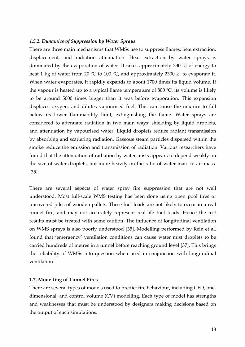
1.5.2. Dynamics of Suppression by Water Sprays There are three main mechanisms that WMSs use to suppress flames: heat extraction, displacement, and radiation attenuation. Heat extraction by water sprays is dominated by the evaporation of water. It takes approximately 330 kJ of energy to heat 1 kg of water from 20 ºC to 100 ºC, and approximately 2300 kJ to evaporate it. When water evaporates, it rapidly expands to about 1700 times its liquid volume. If the vapour is heated up to a typical flame temperature of 800 ºC, its volume is likely to be around 5000 times bigger than it was before evaporation. This expansion displaces oxygen, and dilutes vapourised fuel. This can cause the mixture to fall below its lower flammability limit, extinguishing the flame. Water sprays are considered to attenuate radiation in two main ways: shielding by liquid droplets, and attenuation by vapourised water. Liquid droplets reduce radiant transmission by absorbing and scattering radiation. Gaseous steam particles dispersed within the smoke reduce the emission and transmission of radiation. Various researchers have found that the attenuation of radiation by water mists appears to depend weakly on the size of water droplets, but more heavily on the ratio of water mass to air mass. [35]. There are several aspects of water spray fire suppression that are not well understood. Most full-scale WMS testing has been done using open pool fires or uncovered piles of wooden pallets. These fuel loads are not likely to occur in a real tunnel fire, and may not accurately represent real-life fuel loads. Hence the test results must be treated with some caution. The influence of longitudinal ventilation on WMS sprays is also poorly understood [35]. Modelling performed by Rein et al. found that ‘emergency’ ventilation conditions can cause water mist droplets to be carried hundreds of metres in a tunnel before reaching ground level [37]. This brings the reliability of WMSs into question when used in conjunction with longitudinal ventilation.

1.7. Modelling of Tunnel Fires There are several types of models used to predict fire behaviour, including CFD, one-dimensional, and control volume (CV) modelling. Each type of model has strengths and weaknesses that must be understood by designers making decisions based on the output of such simulations.

14

Fires in tunnels result in complex three-dimensional flow phenomena. Tunnel geometry, ventilation conditions, and other factors interact and result in a range of behaviours. CFD models find a solution to the Navier-Stokes equations using appropriate boundary conditions. The complex physical interactions that occur in tunnel fires can be simultaneously modelled in order to quantify their influence on the overall behaviour. However, the physical behaviour of such problems is not fully understood, and some mathematical assumptions need to be made to obtain solutions. It is important for users to understand these limitations in order to reduce uncertainties to acceptable levels. CFD models are much cheaper to perform than full-scale experiments, and can approximate tunnel fire behaviour with acceptable accuracy when used properly. However, they can be computationally expensive [38]. One-dimensional models divide the tunnel geometry into a series of nodes and branches. It is assumed that the properties are constant over the height at any cross-section in the tunnel. One of the main limitations of one-dimensional models is when there are vertical temperature or velocity gradients. One-dimensional models are relatively simple to use, and are computationally inexpensive [39]. Control volume models work by dividing the tunnel geometry into a series of CVs and then analysing them. The properties throughout each CV are assumed to be constant. Conservation equations are applied in order to predict the properties in each CV. One of the main limitations of CV models occurs when the flow behaviour departs from the conceptual basis on which the model was created. CV models have the advantage of being computationally inexpensive and relatively easy to use [40].

1.8. Problem Statement and Objectives The problem has been introduced above, and can be summarised by the following problem statement: Tunnel designers have recently moved towards fire strategies using water mist systems to control the heat release rates in tunnel fires. However, when designing longitudinal ventilation systems to prevent backlayering, they do not currently account for the additional mass and steam introduced to the tunnel by the water mist system. This thesis aims to quantify the interaction between longitudinal ventilation systems and water mist system operation in tunnel fires.

15

2. METHODOLOGY

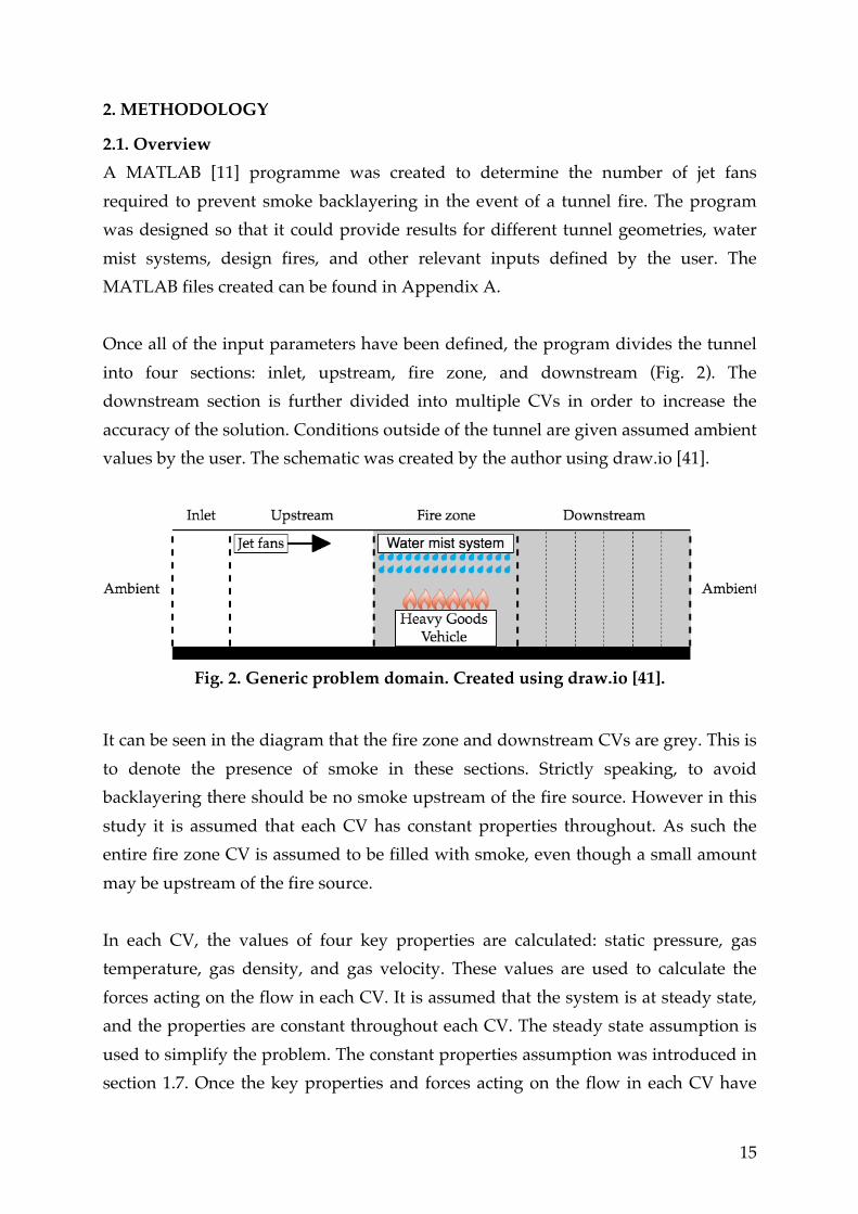
2.1. Overview A MATLAB [11] programme was created to determine the number of jet fans required to prevent smoke backlayering in the event of a tunnel fire. The program was designed so that it could provide results for different tunnel geometries, water mist systems, design fires, and other relevant inputs defined by the user. The MATLAB files created can be found in Appendix A. Once all of the input parameters have been defined, the program divides the tunnel into four sections: inlet, upstream, fire zone, and downstream (Fig. 2). The downstream section is further divided into multiple CVs in order to increase the accuracy of the solution. Conditions outside of the tunnel are given assumed ambient values by the user. The schematic was created by the author using draw.io [41].

Fig. 2. Generic problem domain. Created using draw.io [41].

It can be seen in the diagram that the fire zone and downstream CVs are grey. This is to denote the presence of smoke in these sections. Strictly speaking, to avoid backlayering there should be no smoke upstream of the fire source. However in this study it is assumed that each CV has constant properties throughout. As such the entire fire zone CV is assumed to be filled with smoke, even though a small amount may be upstream of the fire source. In each CV, the values of four key properties are calculated: static pressure, gas temperature, gas density, and gas velocity. These values are used to calculate the forces acting on the flow in each CV. It is assumed that the system is at steady state, and the properties are constant throughout each CV. The steady state assumption is used to simplify the problem. The constant properties assumption was introduced in section 1.7. Once the key properties and forces acting on the flow in each CV have

16

been calculated, a force balance is performed. The calculation procedure is iterated until two conditions are met: the forces acting in the tunnel are balanced, and the upstream velocity is greater than the CVV. The algorithm used to solve the problem is briefly introduced below, with each step explained in more depth later in this chapter.

1. The user defines key parameters of the problem including tunnel dimensions and the HRR in open, still, ambient conditions

2. The CVV is calculated 3. The initial velocity at the inlet portal is set as equal to the CVV, the initial

number of jet fans is set to one, and initial values for other values are defined 4. The HRR is adjusted to account for enclosure effects, forced ventilation, and

suppression by the WMS 5. The key properties and the forces acting are calculated in each CV 6. A force balance is performed on the tunnel 7. If the force balance is negative, another fan is added and the algorithm returns

to step 4 8. If the force balance is positive, the ventilation velocity is increased and the

algorithm returns to step 4 9. If the force balance is sufficiently close to zero, the solution is deemed to have

converged Fig. 3 shows the algorithm in the form of a flow chart. The MATLAB script file “MasterScript” was written to carry out this algorithm and can be found in Appendix A1.

17

Fig. 3. Calculation process. Created using [41].

The following sections aim to explain and justify each part of the algorithm.

2.2. Algorithm

2.2.1. Problem Initialisation The problem is initialised in steps 1-3 defined above. These steps are contained within the MATLAB script file “initialiseProblem”, which can be found in Appendix A2. In step 1, the user specifies a range of relevant parameters. The user specifies these values in the MATLAB script file “Parameters”, which can be found in Appendix A3.

18

Example input values are tabulated in Appendix B. Appropriate values and references are provided for parameters that are likely to be independent of the tunnel, such as the drag coefficient of an average car. In step 2, the CVV is calculated according to (20) proposed by Li et al. [32], repeated below for convenience. It is assumed that the CVV is not reduced due to the effect of blockage as described by Li et al. [32]. This is a conservative assumption, as a larger CVV requires more thrust and hence more fans.

!!"#$∗ = 0.81!∗! ! !"# !∗ ≤ 0.15 !!"#$∗ = 0.43 !"# !∗ > 0.15

(20)

The dimensionless CVV is assumed to be equal to its maximum theoretical value of 0.43. This is again a conservative assumption. As such, it is implicitly assumed that the dimensionless HRR is larger than 0.15. It is reasonable to assume that the dimensionless HRR is this big, as full-scale experiments have demonstrated that very high HRRs can occur in tunnel fires involving HGVs [5]. For example, consider a large road tunnel with a height of 6 m. A HRR of 15 MW is large enough for the dimensionless HRR to exceed 0.15. It has not been demonstrated that WMSs can reliably control HRRs in tunnel fires to 15 MW. As such it was deemed reasonable to conservatively assume that the dimensionless HRR exceeds 0.15. The MATLAB script file “Critical_ventilation_velocity” is used to perform the calculations for step 2 (Appendix A4). In step 3, the upstream velocity is set as equal to the CVV, and the number of fans is set to an initial value of one. Other parameters are given initial values so that the first iteration of the algorithm can be completed. The solution is independent of the initial values given to these other parameters. These operations are contained in the “initialiseProblem” script file.

2.2.2. Heat Release Rate Adjustment The HRR previously defined for open, still, ambient conditions is adjusted to account for enclosure effects, forced ventilation, and suppression by the water mist system. The MATLAB script file used to perform these calculations is called

19

“HeatReleaseRateAdjustment” and can be found in Appendix A5. These calculations also require the use of “interpolateCustom”, which can be found in Appendix A6. The increase in HRR due to enclosure effects was modelled according to Eq. 2 and Eq. 3 proposed by Carvel et al. [16][17][18], repeated below. These equations are only valid if the width of the fire source is less than or equal to half the width of the tunnel.

!!"##$% = !!!"#$ (2)

! = 24 !!!!

!+ 1 (3)

The increase in HRR due to forced ventilation velocity was modelled using the curves proposed by Carvel and Beard [19]. The HRR is increased by a scale factor k according to Eq. 4, repeated below.

!!"#$%&'$"( = !!!"##$% (4)

Carvel proposed sets of k value curves for both the growth phase and for fully involved tunnel fires. It was deemed that the curves for the growth phase were inappropriate as they are inherently temporally dependent, while the model assumes a steady state. A value taken from a growth phase curve represents how much the forced ventilation has increased the growth rate up to a given time in a fire, while a value taken from a fully involved curve represents how much the forced ventilation increases the HRR at its peak. For example, if a k value of 4 is taken from a growth phase curve, this implies that the HRR at a given time is four times larger than it would have been at the same time had there been no forced ventilation. Contrastingly, if a k value of 4 is taken from a fully involved curve, this implies that the HRR reached a peak value four times larger than it would have had there been no forced ventilation. On this basis, it was deemed more appropriate to use the fully involved curves. The curves Carvel proposed were presented with several percentile distributions: 10%, 30%, 50%, expected, 70%, and 90%. For example, a value of 90% estimates an enhancement factor that will be equal to or greater than the actual enhancement

20

factor in 90% of fires. The user specifies which distribution to use. Different curves were presented for one-lane and two-lane tunnels. The user also specifies whether the tunnel being analysed is one-lane or two-lane. The k values were extracted from the curves presented by Carvel and Beard [19] using WebPlotDigitizer [42]. The tabulated k values can be found in Appendix C. The decrease in HRR due to the operation of a WMS was modelled using Eq. (22), as follows:

!!"#$%&'" = !!"#!!"#$%&'$"( (22)

where !!"#$%&'" is the final adjusted HRR and !!"# is how much the HRR is reduced due to WMS operation. This simple model was chosen because the effect of a WMS on the HRR in a tunnel fire is not adequately understood. The actual relationship between WMS operation and HRR reduction may depend on many other factors, including the mass flow density of the WMS, droplet size, and HRR at the time of activation. It is claimed that the operation of a WMS can reduce the HRR to approximately 20-70% of its potential maximum HRR, according to the publicly available test reports [6][43]. The effect of this factor is studied extensively in the results (section 3).

The final result of these operations is !!"#$%&'", which is used for the rest of the calculations in a given iteration of the algorithm. Alternatively, the user can bypass

this part of the algorithm and directly specify a value for !!"#$%&'".

2.2.3. Control Volume Analyses The goal of this section is to present the calculation of the static pressure, temperature, density, and velocity in each CV and the forces acting on the flow. In the inlet section, three assumed values and a form of Bernoulli’s equation are used to determine the four key properties and the forces acting. The temperature and density are assumed to be equal to the ambient values. The temperature is assumed as equal to ambient because there is no external heat source or sink acting on the CV.

21

The density is assumed as equal to ambient using the incompressible flow assumption, as the Mach number in this context will always be well below 0.3. The velocity in the inlet is initially assumed to be equal to the CVV, and is updated later in the algorithm as required. The mass flow rate of air in the tunnel is calculated at the inlet, as follows:

!!"# = !!"#$%!!"##$%!!"#$% = !!!!"##$%!!"#$% (23)

where !!"# is the mass flow rate of air, !!"#$% is the density of air at the inlet, !!"##$% is

the cross sectional area of the tunnel, !!"#$% is the inlet velocity, and !! is the ambient air density. A form of Bernoulli’s equation is then used in order to calculate the static pressure at the inlet portal, as follows:

!!"#$%,!"#$%& = !! −!!"#$%!!"#$%!

2 (24)

where !!"#$%,!"#$%! is the pressure at the inlet portal, and !! is the ambient pressure. This equation gives the pressure at the inlet portal. However, it does not account for pressure losses along the length of the inlet section. Hence the pressure in the inlet CV is calculated as follows:

!!"#$% = !!"#$%,!"#$%& + !!!"##$#,!"#$% (25)

where

!!!"##$#,!"#$% = !1!"#$% + !2!"#$% + !5!!"##$% (26)

!1!"#$% =−!!"#$%2 !!,!"#!!"#$%! !!"#!!"#$,!"#$% (27)

!!"#$,!"#$% = !!"#$%!!"#$$%& (28)

22

!2!"#$% = −! !!"#$%2!!"#$%!!

!!"##$%!!"#$%! (29)

!5 = −!!"!!"#$%2 !!"##$%!!"#$%! (30)

where !!"#$,!"#$% is the number of cars in the inlet section, !!"#$$%& is the car density, and all other parameters are as introduced in section 1.4.3. This method results in the calculated CV pressure being slightly too low. It essentially calculates the pressure at the end of the CV then assumes that is the value throughout the CV. It would be more accurate to assume the pressure in the CV is equal to the average of the start and end values. However, calculating the average value becomes difficult in the later CVs and has negligible impact on the solution obtained. As such, this assumption was made in all of the CVs considered. The code used to perform the inlet calculations can be found in the MATLAB script file “InletCV” (Appendix A7). In the upstream section, it is again assumed that the density is equal to ambient density, as the flow velocity in this context will always result in a Mach number well below 0.3. The temperature is again assumed to be equal to the ambient temperature, as there is no external heat source or sink. The inlet and upstream densities are both equal to the ambient density, and by extension the upstream velocity is equal to the inlet velocity due to the mass balance requirement. The pressure in this CV was calculated as follows:

!!"#$%&'( = !!"#$% + !!!"#$ + !!!"##$#,!"#$%&'( (31)

where

!!!"#$ =!4

!!"##$% (32)

!!!"##$#,!"#$%&'( = !1!"#$%&'( + !2!"#$%&'(!!"##$%

(33)

23

where !1!"#$%&'( and !2!"#$%&'( are calculated the same way as in the inlet CV, and F4 is calculated as follows:

!4 = !!"#$!!"#$%&'(!!"#!!"# !!"# − !!"#$%&'( !! (34)

The code used to perform the above calculations can be found in the MATLAB script file “UpstreamCV” (Appendix A8). In the fire zone section, the mass flow rates of pyrolysis gases is calculated as follows:

!!"#$%"&'&()&*& =!!"#$%&'"!!!,!""

(35)

where !!!,!"" is the effective heat of combustion of the fuel in the tunnel. The mass flow rates of water, steam and water that does not evaporate are calculated as follows:

!!"#$% = !!"#!!! !!"#$%!!"#$!!"##$%!!"##$% (36)

!!"#$% = !!"#$%,!"#$"%$&' + !!"#$%,!"#$%!&'"# (37)

!!"#$%,!"#$ = (1− !!"#$)!!"#$%&%&' (38)

where

!!"#$%,!"#$"%$&' =!!"#!!"#$%&'"

ℎ!"#$%,!"! − ℎ!"#$%,! (39)

!!"#$%,!"#$%!&'"# = !!"#$!!"#$%&%&' (40)

!!"#$%&%&' = !!"#$% − !!"#$%,!"#$"%$&' (41)

where !!"#!!! is the WMS water flux density, !!"#$% is the number of WMS zones,

!!"#$ is the length of one WMS zone, !!"#$%,!"#$"%$&' is the mass flow rate of steam

created by the evaporation of water due to radiation, !!"# is the radiative fraction

(taken as 0.35 [12]), ℎ!"#$%,!"! is the specific enthalpy of steam at 373 K, ℎ!"#$%,! is the

24

specific enthalpy of ambient water, !!"#$%&%&' is the remaining amount of water,

!!"#$%,!"#$%!&'"# is the mass flow rate of steam created by the evaporation of water

due to convection, !!"#$ is the proportion of remaining water evaporated due to

convection, and !!"#$%,!"#$ is the mass flow rate of water that does not evaporate and falls to the ground. It is assumed that all of the radiation energy released by the fire is used to evaporate water. This assumption is made for several reasons. Firstly, water mist has been experimentally observed to strongly attenuate and absorb radiation [35]. Secondly, making this assumption results in higher downstream forces, which is a conservative result in the context of this work. Thirdly, it allows the heat losses model to meet its required boundary condition. The downstream forces acting on the flow are

dependent on the value of the term !!"#$%&'()*!!"#$%&'()*! . By increasing the mass of steam in the air, the value of this term also increases. Increasing the mass of steam in the air also increases the specific ideal gas constant of the mixture. This lowers the density, which causes an increased velocity and hence increases the value of the

!!"#$%&'()*!!"#$%&!"#$! term. The heat losses model used has a boundary condition requiring that the heat transfer by convection to the tunnel surface is equal to the heat transfer by conduction at the surface. For this boundary condition to be valid, the heat transfer by radiation must be negligible. Assuming that all of the radiant heat was attenuated by water mist allows this boundary condition to be met. The presence of water in smoke reduces the emission and transmission of radiation, thus reducing the radiant heat transfer between smoke and the tunnel walls [35]. The amount of water evaporated due to the convective heat release is assumed to

depend on a user specified value for !!"#$. This is a crude assumption, the implications of which are discussed further in section 2.3.1. This value is set to zero by default. It is assumed that the temperature of liquid water suspended in the flow is equal to the temperature in the fire zone. This can lead to a problem for fire zone

temperatures in excess of 100 ºC, as it creates a large energy barrier. Setting !!"#$ to zero essentially means that the system has to provide enough energy to evaporate all of the water if the temperature is to exceed 100 ºC. An attempt was made in section

2.3.1 to calibrate the value of !!"#$ using experimental results.

25

The mass flow rate of gas leaving the fire zone CV is then calculated as follows:

!!"#$%&'$ = !!"#$%&'( +!!"#$ +!!"#$% (42)

An energy balance is solved iteratively in order to determine the four key properties and the forces acting on the CV. The energy balance solved was based on the following steady state form described by Moran and Shapiro [44]:

!!" = 0 = !!" − !!" + !!" ℎ!" +!!"!2 + !!!" − !!"# ℎ!"# +

!!"#!2 + !!!"# (43)

where !!" accounts for heat transferred across the CV boundary, !!" accounts for

work transferred across the CV boundary, ! is the mass flow rate across the CV

boundary, ℎ is the specific enthalpy, ! is the velocity, and ! is the average elevation. The general energy balance equation above was altered into the following form in order to analyse the fire zone CV:

!!" = 0 = !!" − !!" + !!"#$%&'( ℎ!"#$%&'( + !!"#$%&'(!

2 + !!!"#$%&'(

+ !!"#$% ℎ!"#$% +!!"#$%!

2 + !!!"#$%

− !!"#$%&'$ ℎ!"#$%&'$ +!!"#$%&'$!

2 + !!!"#$%&'$

− !!"#$%,!"#$ ℎ!"#$%,!"#$ +!!"#$%&'$!

2 + !!!"#$%,!"#$

(44)

The value of !!" is calculated as follows:

!!" = !!"#$%&'" − !!"##$# (45)

where !!"!"#$%& is the value calculated earlier in the algorithm and !!"##$# is calculated as follows:

26

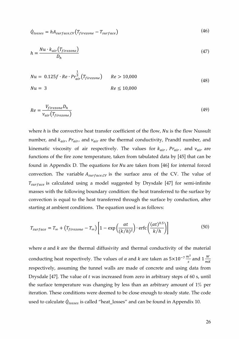
!!"##$# = ℎ!!"#$%&',!" !!"#$%&'$ − !!"#$%&' (46)

ℎ = !" ∙ !!"# !!!"#$%&#!!

(47)

!" = 0.125! ∙ !" ∙ !"!"#!! !!"#$%&'$ !" > 10,000

!" = 3 !" ≤ 10,000 (48)

!" = !!"#!"#$!!!!!"# !!"#$%&'$

(49)

where ℎ is the convective heat transfer coefficient of the flow, !" is the flow Nussult

number, and !!"#, !"!"#, and !!"# are the thermal conductivity, Prandtl number, and

kinematic viscosity of air respectively. The values for !!"# , !"!"# , and !!"# are functions of the fire zone temperature, taken from tabulated data by [45] that can be

found in Appendix D. The equations for !" are taken from [46] for internal forced

convection. The variable !!"#$%&',!" is the surface area of the CV. The value of

!!"#$%&' is calculated using a model suggested by Drysdale [47] for semi-infinite masses with the following boundary condition: the heat transferred to the surface by convection is equal to the heat transferred through the surface by conduction, after starting at ambient conditions. The equation used is as follows:

!!"#$%&' = !! + !!"#$%&'$ − !! 1− exp !"(! ℎ)! ∙ erfc !" !.!

! ℎ (50)

where ! and ! are the thermal diffusivity and thermal conductivity of the material

conducting heat respectively. The values of ! and ! are taken as 5×10!! !!

! and 1 !!"

respectively, assuming the tunnel walls are made of concrete and using data from

Drysdale [47]. The value of ! was increased from zero in arbitrary steps of 60 s, until the surface temperature was changing by less than an arbitrary amount of 1% per iteration. These conditions were deemed to be close enough to steady state. The code

used to calculate !!"##$# is called “heat_losses” and can be found in Appendix 10.

27

The value of !!" is calculated as follows:

!!" = !!"#$%&'$ !1!"#$%&'$ + !2!"#$%&'$ + !6 (51)

The values of ℎ!"#$%&'( and !!"#$%&'( were calculated previously. The value of

!!"#$%&'( is equal to half the tunnel height, as this is the average elevation. The value

of ℎ!"#$% is taken from tabulated data by the National Institute of Standards and Technology (NIST) [48] and is assumed to be at ambient conditions of 20 ºC and

101,325 Pa. The value of !!"#$% is based on properties of the WMS, and is calculated as follows:

!!"#$% =!!"##$%!!"#$%!!"#$%!!"##$%

(52)

The value of !!"#$% is equal to the height of the tunnel as it is assumed that the WMS

is located at ceiling level. The value of ℎ!"#$%&'$ is calculated as follows:

ℎ!"#$%&'$ = ℎ!"#$%&'$,!"#!!"# + !!"#$%"&'&()&*&

!!"#$%&'()*+ ℎ!!"#$%&#,!"#$%

!!"#$%!!"#$%&'()*

(53)

The values of ℎ!"#$%&'$,!"# and ℎ!"#$%&'$,!"#$% are found using functions called “spec_ent_air” and “spec_ent_steam”, which look up tabulated values for the specific enthalpy based on an input temperature. Where required these functions will linearly interpolate to find more accurate values. The temperature of the air is equal to the fire zone temperature. The temperature of the steam is taken as the larger of the fire zone temperature or 100 ºC. The codes can be found in Appendix 11 and Appendix 12. The specific enthalpy values of air and steam are taken from Moran and Shapiro [44] and NIST [48] respectively and can be found in Appendix E and F. The mass flow rate of pyrolysis gases is included with the air term, as it is difficult to

estimate the specific enthalpy of pyrolysis gases. The value of !!"#$%&'$ is calculated as follows:

28

!!"#$%&'$ =!!"#$%&'$

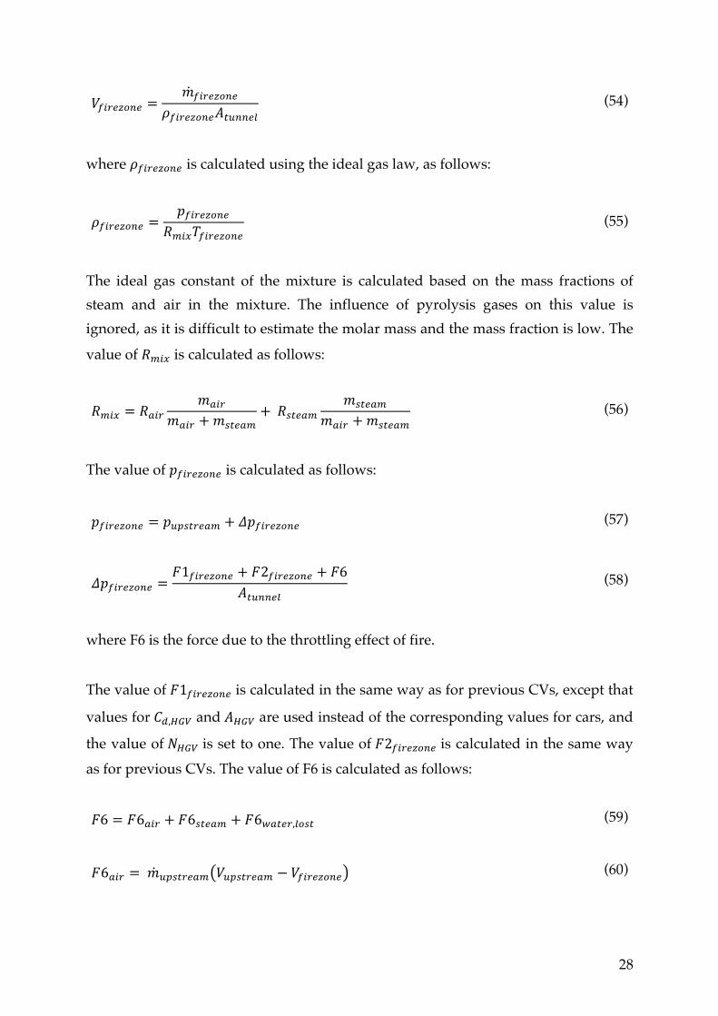
!!"#$%&'$!!"##$% (54)

where !!"#$%&'$ is calculated using the ideal gas law, as follows:

!!"#$%!"# =!!"#$%&'$

!!"#!!"#$%&'$ (55)

The ideal gas constant of the mixture is calculated based on the mass fractions of steam and air in the mixture. The influence of pyrolysis gases on this value is ignored, as it is difficult to estimate the molar mass and the mass fraction is low. The

value of !!"# is calculated as follows:

!!"# = !!"#!!"#

!!"# +!!"#$%+ !!"#$%

!!"#$%!!"# +!!"#!"

(56)

The value of !!"#$%&'$ is calculated as follows:

!!"#$%&'$ = !!"#$%&'( + !!!"#$%&'$ (57)

!!!"#$%&'$ =!1!"#$%&'$ + !2!"#$%&!" + !6

!!"##$% (58)

where F6 is the force due to the throttling effect of fire.

The value of !1!"#$%&'$ is calculated in the same way as for previous CVs, except that

values for !!,!"# and !!"# are used instead of the corresponding values for cars, and

the value of !!"# is set to one. The value of !2!"#$%&'$ is calculated in the same way as for previous CVs. The value of F6 is calculated as follows:

!6 = !6!"# + !6!"!"# + !6!"#$%,!"#$ (59)

!6!"# = !!"#$%&'( !!"#$%&'( − !!"#$%&'$ (60)

29

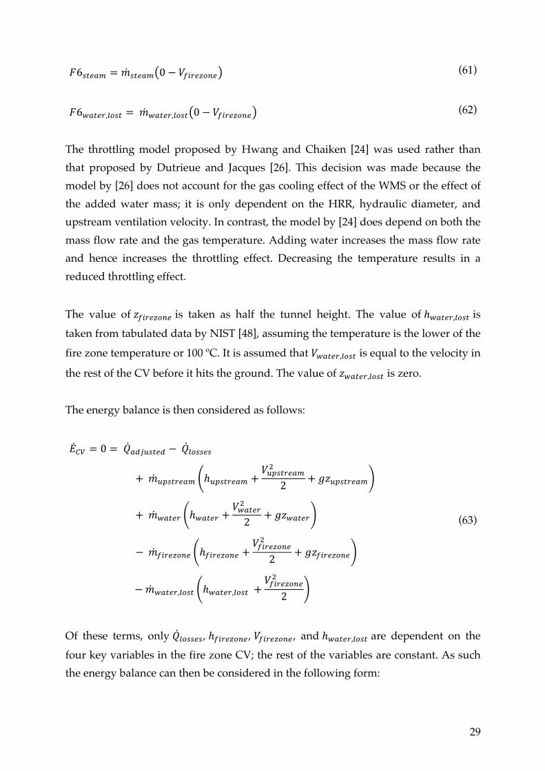
!6!"#$% = !!"#$% 0− !!"#$%&'$ (61)

!6!"#$%,!"#$ = !!"#$%,!"#$ 0− !!"#$%&'$ (62)

The throttling model proposed by Hwang and Chaiken [24] was used rather than that proposed by Dutrieue and Jacques [26]. This decision was made because the model by [26] does not account for the gas cooling effect of the WMS or the effect of the added water mass; it is only dependent on the HRR, hydraulic diameter, and upstream ventilation velocity. In contrast, the model by [24] does depend on both the mass flow rate and the gas temperature. Adding water increases the mass flow rate and hence increases the throttling effect. Decreasing the temperature results in a reduced throttling effect.

The value of !!"#$%&'$ is taken as half the tunnel height. The value of ℎ!"#$%,!"#$ is taken from tabulated data by NIST [48], assuming the temperature is the lower of the

fire zone temperature or 100 ºC. It is assumed that !!"#$%,!"#$ is equal to the velocity in

the rest of the CV before it hits the ground. The value of !!"#$%,!"#$ is zero. The energy balance is then considered as follows:

!!" = 0 = !!"#$%&'" − !!"##$#

+ !!"#$%&'( ℎ!"#$%&'( + !!"#$%&'(!

2 + !!!"#$%&'(

+ !!"#$% ℎ!"#$% +!!"#$%!

2 + !!!"#$%

− !!"#$%&'$ ℎ!"#$%&'$ +!!"#$%&'$!

2 + !!!!"#$%&#

− !!"#$%,!"#$ ℎ!"#$%,!"#$ + !!"#$%&'$!

2

(63)

Of these terms, only !!"##$#, ℎ!"#$%&'$, !!"#$%&'$, and ℎ!"#$!,!"#$ are dependent on the four key variables in the fire zone CV; the rest of the variables are constant. As such the energy balance can then be considered in the following form:

30

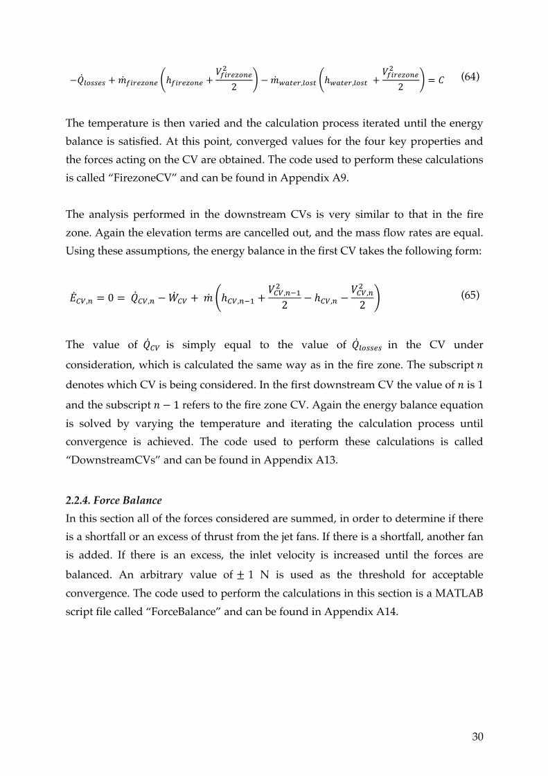
−!!"##$# +!!"#$%&'$ ℎ!"#$%&'$ +!!"#$%&'$!

2 −!!"#$%,!"#$ ℎ!"#$%,!"#$ +!!"#$%&'$!

2 = ! (64)

The temperature is then varied and the calculation process iterated until the energy balance is satisfied. At this point, converged values for the four key properties and the forces acting on the CV are obtained. The code used to perform these calculations is called “FirezoneCV” and can be found in Appendix A9. The analysis performed in the downstream CVs is very similar to that in the fire zone. Again the elevation terms are cancelled out, and the mass flow rates are equal. Using these assumptions, the energy balance in the first CV takes the following form:

!!",! = 0 = !!",! −!!" + ! ℎ!",!!! +!!",!!!!

2 − ℎ!",! −!!",!!

2 (65)

The value of !!" is simply equal to the value of !!"##$# in the CV under

consideration, which is calculated the same way as in the fire zone. The subscript !

denotes which CV is being considered. In the first downstream CV the value of ! is 1

and the subscript ! − 1 refers to the fire zone CV. Again the energy balance equation is solved by varying the temperature and iterating the calculation process until convergence is achieved. The code used to perform these calculations is called “DownstreamCVs” and can be found in Appendix A13.

2.2.4. Force Balance In this section all of the forces considered are summed, in order to determine if there is a shortfall or an excess of thrust from the jet fans. If there is a shortfall, another fan is added. If there is an excess, the inlet velocity is increased until the forces are

balanced. An arbitrary value of ± 1 N is used as the threshold for acceptable convergence. The code used to perform the calculations in this section is a MATLAB script file called “ForceBalance” and can be found in Appendix A14.

31

2.3. Model Validation

2.3.1 Overview The model is made up of several components that are combined with the aim of simulating complex behaviour. Due to the specific nature of the problem and the high cost of full-scale tunnel fire tests, there is no experimental data that is fully applicable for validating the model. As such, the model’s reliability is validated by comparing applicable data with the results obtained using different components of the model. The model was validated using experimental data for the downstream temperatures in tunnel fires with suppression, and simulation results for the number of fans required to prevent backlayering in an unsuppressed tunnel.

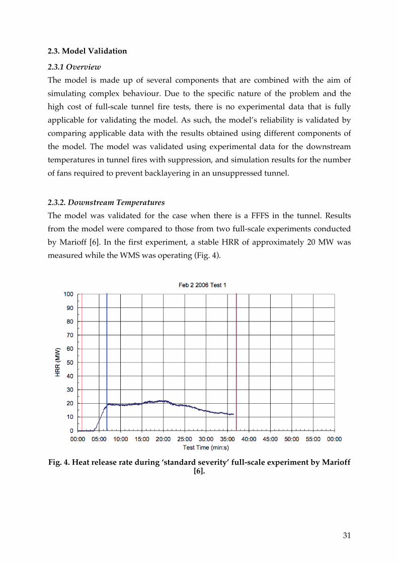
2.3.2. Downstream Temperatures The model was validated for the case when there is a FFFS in the tunnel. Results from the model were compared to those from two full-scale experiments conducted by Marioff [6]. In the first experiment, a stable HRR of approximately 20 MW was measured while the WMS was operating (Fig. 4).

Fig. 4. Heat release rate during ‘standard severity’ full-scale experiment by Marioff

[6].

32

The temperatures 25-30 m downstream of the fire can be seen in Fig. 5. The green line is the temperature measured 1.5 m above the ground, the blue at 3 m, and the red at ceiling level. It can be seen that the temperature is approximately 45-60 ºC throughout the cross section. This shows that the 1D model assumption is appropriate when a WMS limits the HRR to a steady state; it is reasonable to assume constant properties throughout the height of the cross section in this case.

Fig. 5. Temperatures at different heights during ‘standard severity’ full-scale

experiment conducted by Marioff [6].

The tunnel used for these experiments was 5.2 m high, 9.5 m wide, and 600 m long. The HRR was assumed to be a constant 20 MW for validating the model. The radiative fraction was set to 0.35. The forced ventilation velocity was 2-3 m/s. A value of 2.5 m/s was used in the model. The location of the fire was not specified, so it was assumed to be in the middle of the tunnel. The specifications of the WMS used in these experiments were not explicitly reported. However, these experiments were used as the basis for specifying the WMS used in the Madrid M30 road tunnel. The WMS installed in the M30 tunnel is designed to provide an average water flux

density of 0.533 l/min/m3 over three zones with length of 24 m each [8]. Based on this, it was assumed that the WMS used in testing had the same average water flux density, zone length, and number of zones.

33

The model was slightly modified in order to accommodate these input values. The script file “HeatReleaseRateAdjustment” was deactivated; a constant HRR of 20 MW was used instead. The inlet velocity was set to a constant 2.5 m/s; it was not altered in the script “ForceBalance”. Using these inputs, the model gave a temperature of 64 ºC in a CV 25-30 m downstream of the fire. This is close to the range measured

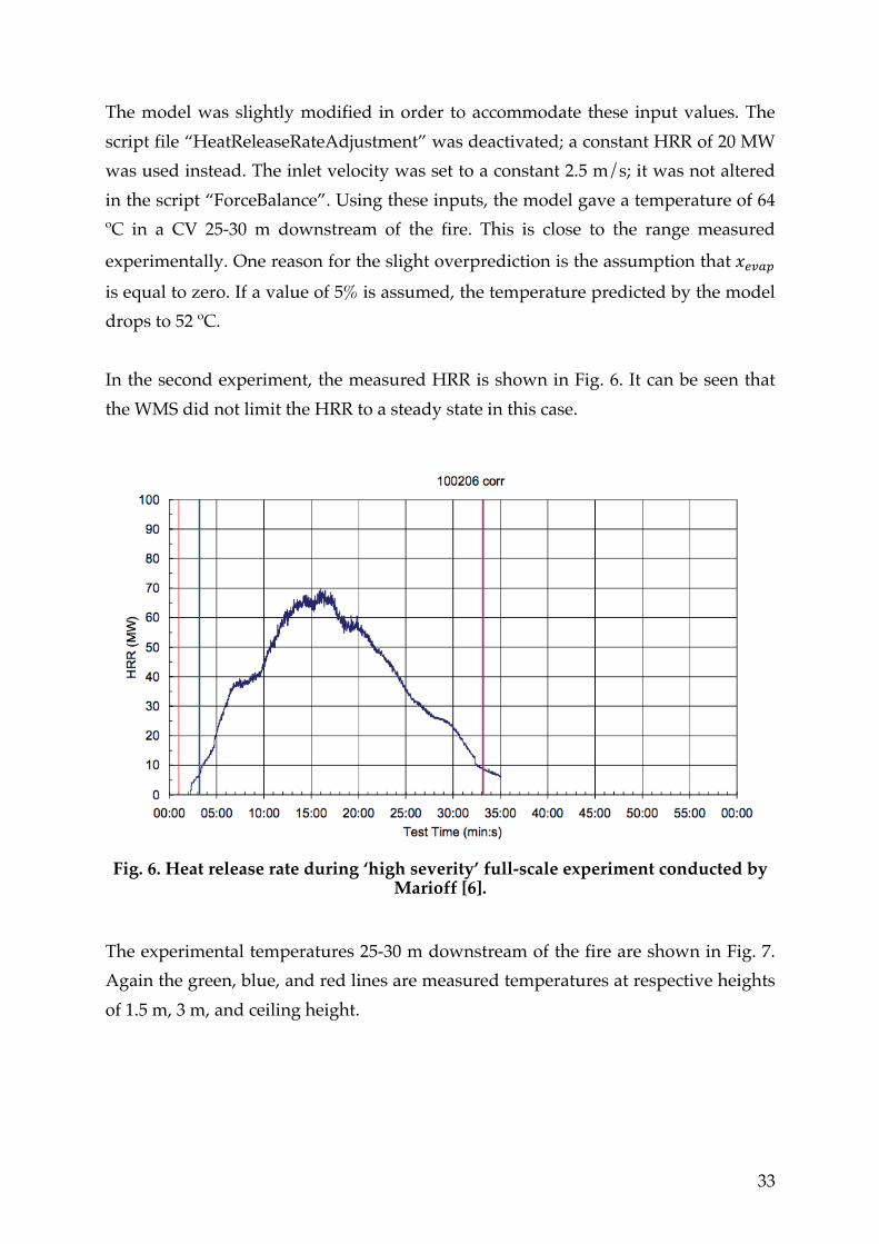
experimentally. One reason for the slight overprediction is the assumption that !!"#$ is equal to zero. If a value of 5% is assumed, the temperature predicted by the model drops to 52 ºC. In the second experiment, the measured HRR is shown in Fig. 6. It can be seen that the WMS did not limit the HRR to a steady state in this case.

Fig. 6. Heat release rate during ‘high severity’ full-scale experiment conducted by

Marioff [6].

The experimental temperatures 25-30 m downstream of the fire are shown in Fig. 7. Again the green, blue, and red lines are measured temperatures at respective heights of 1.5 m, 3 m, and ceiling height.

34

Fig. 7. Temperatures at different heights during ‘high severity’ full-scale

experiment conducted by Marioff [6].

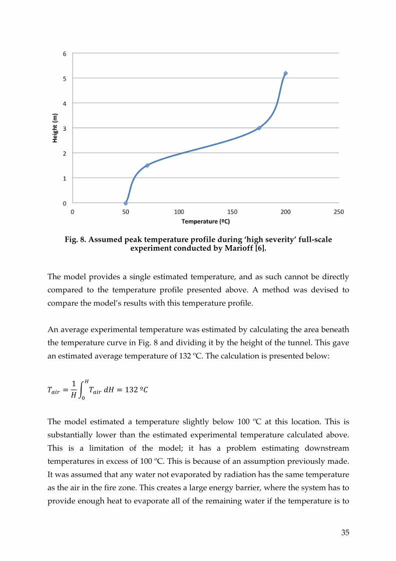
It can be seen that the temperature is not constant over the height of the tunnel. This suggests that the 1D model assumption is flawed when the WMS does not control the HRR of the fire. However, this data can still be of some use for comparison to the results of the model. This was done by assuming a steady state HRR of 65 MW, approximating the period from 12-18 min in Fig. 6. The temperatures at the ceiling, 3 m, and 1.5 m were estimated using the peak values in Fig. 7. These values occur at approximately 18 min, corresponding to the time when the HRR began to decrease. These were taken as 200 ºC, 175 ºC, and 70ºC respectively. The temperature at the ground level was assumed to be 50 ºC. Based on these assumptions, the temperature profile in the tunnel was assumed to have the following form (Fig. 8).

35

Fig. 8. Assumed peak temperature profile during ‘high severity’ full-scale

experiment conducted by Marioff [6].

The model provides a single estimated temperature, and as such cannot be directly compared to the temperature profile presented above. A method was devised to compare the model’s results with this temperature profile. An average experimental temperature was estimated by calculating the area beneath the temperature curve in Fig. 8 and dividing it by the height of the tunnel. This gave an estimated average temperature of 132 ºC. The calculation is presented below:

!!"# =1! !!"# !"

!

!= 132 º!

The model estimated a temperature slightly below 100 ºC at this location. This is substantially lower than the estimated experimental temperature calculated above. This is a limitation of the model; it has a problem estimating downstream temperatures in excess of 100 ºC. This is because of an assumption previously made. It was assumed that any water not evaporated by radiation has the same temperature as the air in the fire zone. This creates a large energy barrier, where the system has to provide enough heat to evaporate all of the remaining water if the temperature is to

36

exceed 100 ºC. If it is assumed that the remaining water reaches a temperature of 100 ºC but none evaporates, the model estimates a temperature of 176 ºC at this location. This is substantially higher than the experimental result. This suggests that the model can bound the solution, which is a useful result. It was found that 18% of the remaining water would have to evaporate for the model to give a temperature of 132

ºC. With more experimental data, the value of !!"#$ could be calibrated to more accurately predict downstream temperatures. Based on these results, it was concluded that the model is valid for predicting gas temperatures up to 100 ºC with the evaporation proportion set to 0%. The general trends predicted by the model were also deemed to have been validated, although caution should be exercised when considering temperatures above 100 ºC.

2.3.3. Backlayer Prevention The final result of the model is to calculate how many fans are required to prevent backlayering for a given set of input values. Consequently the model’s ability to accurately do this must be verified. The most convenient way to do this is by comparing the results of this model with those predicted by other models. The work of Carvel et al. [23] presented the number of fans required to prevent backlayering under different circumstances. The results of Carvel et al. [23] will be used to verify that this model can provide accurate results. Carvel et al. [23] used a tunnel 8 m high, 6.5 m wide, and 100 m long for their simulations. There was no suppression by a WMS or otherwise. The centre of the fire was positioned 32 m from the upstream portal and 68 m from the downstream portal. Seven fans were used. The fans were modelled as 0.5 x 0.5 m squares with zero thickness, producing an outlet velocity of 35 m/s. The upstream ventilation velocity was set to the critical value of 3.4 m/s for simulations where the HRR was greater than the critical dimensionless HRR of 0.15, which in this case is all fires with a HRR of 30 MW or more. The HRR was varied from 10-90 MW in steps of 10 MW. The fire source was generally 3 m wide x 4 m long x 1 m high. Simulations were conducted with the fans located at 25 m and 50 m from the fire, and with varying fire areas. Table 1 compares the results of the model with those found by Carvel et al. for fires with HRRs 30 MW or more. Simulation 1 shows the results with the fans located 25 m from the fire, and standard fire area. Simulation 2 shows the results with the fans 50 m from the fire and using the standard fire area. Simulation 3 shows the

37

results with the fans 50 m from the fire and varying the fire area. Where the table says N/A, it is because the seven fans used by Carvel et al. were not sufficient to prevent backlayering. The model has the ability to predict how many fans are required in these more extreme cases.

Table 1. Number of fans required to prevent backlayering. Results of the model and FDS simulations by Carvel et al. [23]

HRR (MW) Model Simulation 1 Simulation 2 Simulation 3 30 4 3 3 3 40 4 4 4 4 50 5 4 5 4 60 5 5 5 5 70 6 5 5 5 80 6 N/A 6 6 90 6 N/A 7 N/A

It can be seen that the model provides similar results to those obtained by Carvel et al. [23]. Based on this, it was deemed that the model provides a reasonable level of accuracy when predicting the number of fans required to prevent backlayering.

38

3. RESULTS AND DISCUSSION

3.1. Overview A case study was performed on a 6 m wide x 6 m high x 600 m long tunnel in keeping with the work done by Looi [9]. Initially, the tunnel was considered without a fire and without WMS operation. This was to demonstrate the effect of aerodynamic resistance, friction resistance, portal pressure difference and inlet flow separation resistance. The tunnel was then considered for a range of unsuppressed fires. This was to demonstrate the throttling effect and the impact of increased downstream temperatures on the other forces. The tunnel was then considered with WMS operation. The influence of the WMS is analysed and discussed.

3.2. Case Study

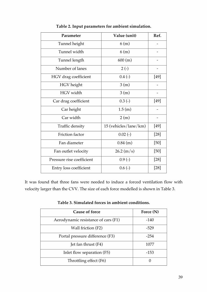
3.2.1. Ambient Conditions The model was used to analyse the tunnel without any fire in the tunnel and without a WMS in operation. This was done to provide baseline values of the different forces acting in the tunnel, for comparison with the corresponding values in the cases with fire in the tunnel. The relevant inputs for this simulation are summarised in Table 2. The number of lanes was set to two in order to determine the number of cars in the tunnel. Drag coefficients for an HGV and an average car were taken based on values from Colella [49]. According to Colella, traffic density during morning rush hour ranges from 8-23 vehicles/lane/km [49]. Based on this, a value of 15 vehicles/lane/km was chosen. The fan diameter and outlet velocity used were specified by Pollrich [50], and are the same as those used by Looi [9]. Jang and Chen specified appropriate values of 0.9 and 0.6 for the pressure rise coefficient and the entry loss coefficient respectively [28].

39

Table 2. Input parameters for ambient simulation.

Parameter Value (unit) Ref.

Tunnel height 6 (m) -

Tunnel width 6 (m) -

Tunnel length 600 (m) -

Number of lanes 2 (-) -

HGV drag coefficient 0.4 (-) [49]

HGV height 3 (m) -

HGV width 3 (m) -

Car drag coefficient 0.3 (-) [49]

Car height 1.5 (m) -

Car width 2 (m) -

Traffic density 15 (vehicles/lane/km) [49]

Friction factor 0.02 (-) [28]

Fan diameter 0.84 (m) [50]

Fan outlet velocity 26.2 (m/s) [50]

Pressure rise coefficient 0.9 (-) [28]

Entry loss coefficient 0.6 (-) [28]

It was found that three fans were needed to induce a forced ventilation flow with velocity larger than the CVV. The size of each force modelled is shown in Table 3.

Table 3. Simulated forces in ambient conditions.

Cause of force Force (N)

Aerodynamic resistance of cars (F1) -140

Wall friction (F2) -529

Portal pressure difference (F3) -254

Jet fan thrust (F4) 1077

Inlet flow separation (F5) -153

Throttling effect (F6) 0

40

Table 3 shows that wall friction was the dominant mode of flow resistance in the tunnel. The aerodynamic resistance of cars, portal pressure difference, and inlet flow separation all caused sizeable drag forces that the fans needed to overcome. As expected, the throttling force was zero.

3.2.2. Unsuppressed Fires The model was used to analyse the tunnel with a range of HRRs. The script file “HeatReleaseRateAdjustment” was bypassed, and HRRs ranging from 2-100 MW in steps of 2 MW were directly specified. Other inputs are shown in Table 4. The other inputs were the same as those specified in Table 2.

Table 4. Inputs parameters for unsuppressed fire simulations.

Parameter Value (unit) Ref.

Inlet CV length 100 (m) -

Upstream CV length 185 (m) -

Fire zone CV length 30 (m) -

Total downstream length 285 (m) -

Number of downstream CVs 30 -

Radiative fraction 0.35 (-) [43]

41

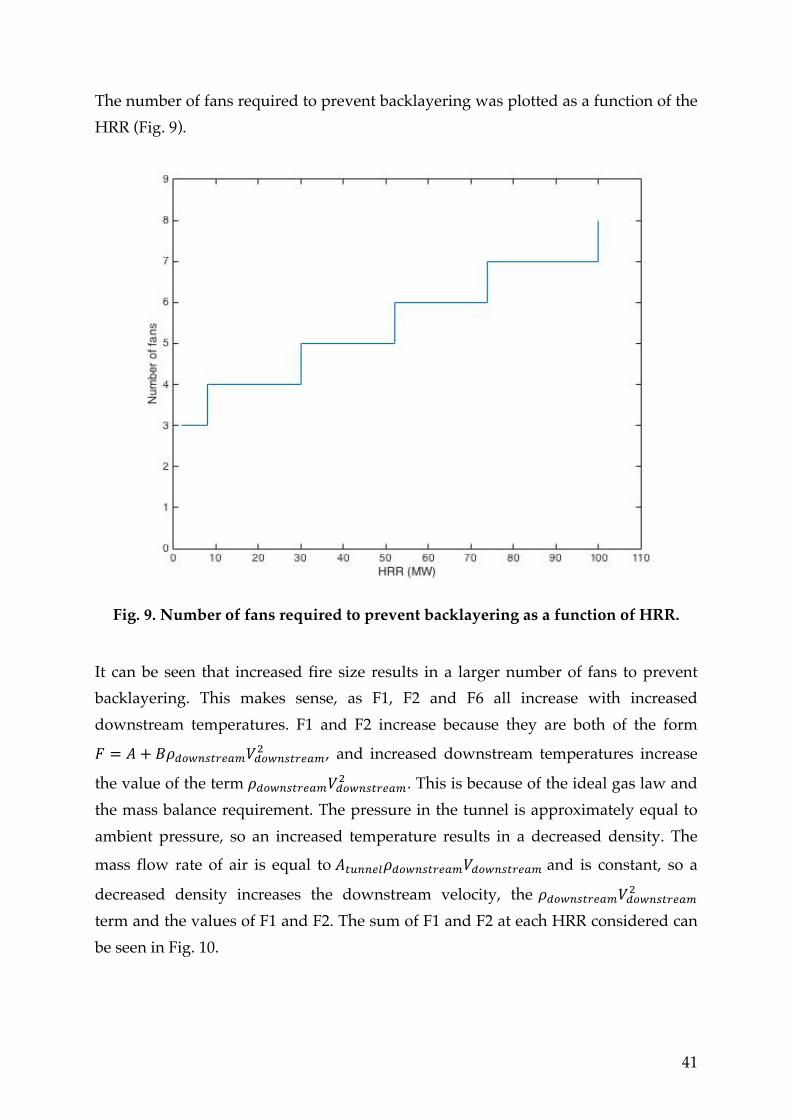
The number of fans required to prevent backlayering was plotted as a function of the HRR (Fig. 9).

Fig. 9. Number of fans required to prevent backlayering as a function of HRR.

It can be seen that increased fire size results in a larger number of fans to prevent backlayering. This makes sense, as F1, F2 and F6 all increase with increased downstream temperatures. F1 and F2 increase because they are both of the form

! = ! + !!!"#$%&'()*!!"#$%&'()*! , and increased downstream temperatures increase

the value of the term !!"#$%&'()*!!"#$%&'()*! . This is because of the ideal gas law and the mass balance requirement. The pressure in the tunnel is approximately equal to ambient pressure, so an increased temperature results in a decreased density. The

mass flow rate of air is equal to !!"##$%!!"#$%&'()*!!"#$%&'()* and is constant, so a

decreased density increases the downstream velocity, the !!"#$%&'()*!!"#$%&'()*! term and the values of F1 and F2. The sum of F1 and F2 at each HRR considered can be seen in Fig. 10.

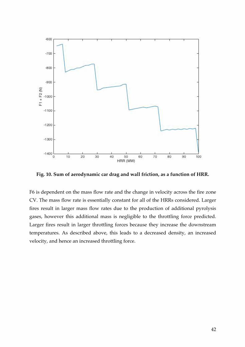
42

Fig. 10. Sum of aerodynamic car drag and wall friction, as a function of HRR.

F6 is dependent on the mass flow rate and the change in velocity across the fire zone CV. The mass flow rate is essentially constant for all of the HRRs considered. Larger fires result in larger mass flow rates due to the production of additional pyrolysis gases, however this additional mass is negligible to the throttling force predicted. Larger fires result in larger throttling forces because they increase the downstream temperatures. As described above, this leads to a decreased density, an increased velocity, and hence an increased throttling force.

43

The forces for selected HRRs are shown in Table 5.

Table 5. Simulated forces for different HRRs.

Force (N)

Cause of force 0 MW 50 MW 100 MW

Aerodynamic resistance of cars (F1) -140 -201 -312

Wall friction (F2) -529 -713 -1080

Portal pressure difference (F3) -254 -236 -277

Jet fan thrust (F4) 1077 1805 2854

Inlet flow separation (F5) -153 -142 -166

Throttling effect (F6) 0 -506 -1028

It can generally be seen that as the HRR increases, the magnitude of each force increases. There are some exceptions to this trend. It can be seen that the values of F3 and F5 for the 50 MW simulation are lower than those for the 0 MW simulation. This is due to the discrete number of fans. The model finds the minimum number of fans required to prevent backlayering, but this results in a surplus of thrust. The model increases the inlet velocity until increased resistance balances the excess thrust. The decrease observed in F3 and F5 between the 0 MW and 50 MW simulations is because the 0 MW simulation had a larger excess of thrust. This resulted in a new inlet velocity higher than that calculated for the 50 MW simulation. This effect can be observed in Fig. 11.

44

Fig. 11. Force due to inlet flow separation as a function of the HRR.

It can be seen that the magnitude of F5 decreases steadily until another fan is added, at which point there is a sudden increase in magnitude. The peak values at the top of the graph are all very similar; this is because they occur when the force balance is approaching zero. The reason for the small differences observed in these values is the convergence criterion set. The solution convergence was deemed acceptable for an absolute force balance of less than 10 N. The peaks at the bottom of the graph are decreasing in magnitude; this is because the solution becomes more sensitive to velocity as the HRR increases. This is again because the downstream forces depend

on the !!"#$%&'()*!!"#$%&'()*! term. The velocity is increased because the density is decreased; the density is decreased because the temperature is increased at an essentially constant pressure. The temperature increases approximately linearly with increased HRR; this is because the specific heat capacity of air is essentially constant over a wide range of temperatures. This linearly increase in temperature with increasing HRR is shown by Fig. 12, which shows the temperature calculated by the model at the middle of the downstream section.

45

Fig. 12. Temperature at the middle of the downstream section for different HRRs.

The small drops in temperature at HRRs of approximately 30 MW, 50 MW, 70 MW, and 100 MW are due to the addition of a fan at these points. This results in an increased inlet velocity, and hence an increased mass flow rate of air. A higher mass flow rate of air with the same amount of energy results in lower temperatures. The results presented in this section appear to demonstrate that higher downstream temperatures require more fans to prevent backlayering. This trend is clearly demonstrated in Fig. 13.

46

Fig. 13. Number of fans required to prevent backlayering, as a function of

temperature at the centre of the downstream section.

Fig. 13 shows that the number of fans increases as the downstream temperature increases. It also shows the downstream temperature decreasing immediately after a fan is added. For example, the temperature increases from approximately 380 ºC to 520 ºC while the number of fans is set to 7, but decreases to about 500 ºC as soon as another fan is added. The main reason for this is again the increased mass flow rate of air reducing the average gas temperature. It can be concluded from the results presented in this section that the downstream temperature has a large influence on the predicted number of jet fans necessary to prevent backlayering. Using the model for unsuppressed fires has limitations that must be taken into account. The equations used to model heat losses through the tunnel walls are not suited to unsuppressed fires, as they assume the radiation heat transfer to the tunnel walls is negligible. This is not accurate for unsuppressed tunnel fires; a large amount of radiant heat will be transferred to the walls. Realistically, this would result in lower temperatures downstream than were calculated using this model. Higher

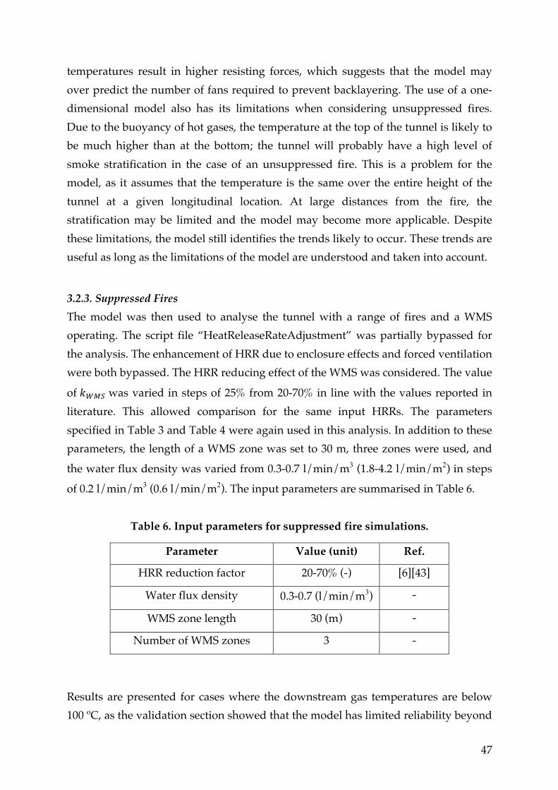
47

temperatures result in higher resisting forces, which suggests that the model may over predict the number of fans required to prevent backlayering. The use of a one-dimensional model also has its limitations when considering unsuppressed fires. Due to the buoyancy of hot gases, the temperature at the top of the tunnel is likely to be much higher than at the bottom; the tunnel will probably have a high level of smoke stratification in the case of an unsuppressed fire. This is a problem for the model, as it assumes that the temperature is the same over the entire height of the tunnel at a given longitudinal location. At large distances from the fire, the stratification may be limited and the model may become more applicable. Despite these limitations, the model still identifies the trends likely to occur. These trends are useful as long as the limitations of the model are understood and taken into account.

3.2.3. Suppressed Fires The model was then used to analyse the tunnel with a range of fires and a WMS operating. The script file “HeatReleaseRateAdjustment” was partially bypassed for the analysis. The enhancement of HRR due to enclosure effects and forced ventilation were both bypassed. The HRR reducing effect of the WMS was considered. The value

of !!"# was varied in steps of 25% from 20-70% in line with the values reported in literature. This allowed comparison for the same input HRRs. The parameters specified in Table 3 and Table 4 were again used in this analysis. In addition to these parameters, the length of a WMS zone was set to 30 m, three zones were used, and

the water flux density was varied from 0.3-0.7 l/min/m3 (1.8-4.2 l/min/m2) in steps

of 0.2 l/min/m3 (0.6 l/min/m2). The input parameters are summarised in Table 6.

Table 6. Input parameters for suppressed fire simulations.

Parameter Value (unit) Ref.

HRR reduction factor 20-70% (-) [6][43]

Water flux density 0.3-0.7 (l/min/m3) -

WMS zone length 30 (m) -

Number of WMS zones 3 -

Results are presented for cases where the downstream gas temperatures are below 100 ºC, as the validation section showed that the model has limited reliability beyond

48

this temperature. The proportion of remaining water evaporating was set to 0%, again due to the results of the validation section. The model performed well when the gas temperatures were below 100 ºC and the proportion of water evaporating was 0%, so presenting the results of similar cases was deemed the most reasonable approach. The estimated number of fans required to prevent backlayering can be seen in Fig. 14-19. The HRR on the x-axis is the ‘unadjusted’ HRR. This corresponds to the HRR

used in section 3.2.2. This HRR is then multiplied by the appropriate !!"# value in order to find the number of fans required to prevent backlayering at this ‘unadjusted’ HRR. The results were divided into six graphs for clarity. The lines were slightly vertically shifted so that they can be seen more easily. In each graph, the value of

either !!"# or the water flux density (denoted WFD) was kept constant while the other was varied.

Fig. 14. Number of fans required with an HRR reduction factor of 0.7.

49

Fig. 15. Number of fans required with an HRR reduction factor of 0.45.

Fig. 16. Number of fans required with an HRR reduction factor of 0.2.

50

Several observations can be made from looking at these graphs. Fig. 14-16 show that increasing the water flux density increases the number of fans required to prevent backlayering up to heat release rates of approximately 15 MW. In all three of the graphs, the lines representing WMS operation never increase beyond four fans, whereas the blue line representing an unsuppressed fire reaches five fans at approximately 29 MW. It was estimated that the blue line ‘overtook’ the other three lines at an average value of approximately 15 MW. The purple line is always at four fans, while the other lines only reach this level at increased HRRs. The purple line represents the highest water flow rate. The larger mass of water introduced into the tunnel was determined to be the reason that more fans were required. This increased mass resulted in an increased thrust requirement to accelerate it to the velocity of the flow in the fire zone. The throttling force in the model represented this behaviour. The throttling equation depends on the mass flow rate in the fire zone and the change in velocity of this mass flow rate. The average longitudinal velocity of the water was assumed to be zero upon entry into the tunnel, and the final velocity was assumed to be equal to the calculated fire zone flow velocity. This inertial resistance dominates the model at lower HRRs, before being surpassed by heat-induced resistances at higher HRRs. At higher HRRs, the mechanisms previously described begin to dominate. Increased temperatures lead to decreased densities, increased velocities, and increased downstream forces. This is why the blue line increases to five fans while the others do not: the downstream temperatures in unsuppressed fires are larger than those in suppressed fires. If the HRR were to be increased further beyond the 30 MW shown in the graphs, the blue line would start to diverge further from the others due to these temperature-induced forces.

51

Fig. 17. Number of fans required with a WFD of 0.3 l/min/m3.

Fig. 18. Number of fans required with a WFD of 0.5 l/min/m3.

52

Fig. 19. Number of fans required with a WFD of 0.7 l/min/m3.

Fig. 17-19 show that decreasing the value of !!"# reduces the number of fans required to prevent backlayering. The purple line represents the lowest value of

!!"# and is the last to increase to four fans, apart from in the case with a water flux

density of 0.7 l/min/m3. In this case, the inertia of the high mass of water causes the line to sit at four fans even at low HRRs. The orange line represents the case with the

highest !!"# value, so it makes sense that this line is consistently the first one to

reach four fans. The higher !!"# value results in higher temperatures, so the temperature driven forces begin to dominate earlier for this simulation than for the purple line. Fig. 17 shows the purple line only reaching four fans at a HRR close to 30 MW. This also suggests that

53

4. CONCLUSIONS

A one-dimensional control volume model was implemented in MATLAB in order to analyse the relationship between the operation of a water mist system and the number of jet fans required to prevent smoke backlayering in a tunnel fire. It was found that a water mist system has a mixed effect on the number of fans required. At heat release rates lower than approximately 15 MW, it was found that the water mist system increased the number of fans required. This was deemed to be due to resistance generated in accelerating the relatively large mass of water to the speed of the fire zone flow. For heat release rates larger than 15 MW, it was found that a water mist system reduced the number of fans required. It was found that two main mechanisms were responsible for this reduced number of fans: heat release rate reduction and downstream gas cooling. The forces acting against the jet fans were found to be heavily influenced by the downstream temperatures generated by the fire. Hence when a water mist system is activated, the magnitudes of these forces are likely to be reduced. The model could be improved in many ways. The relationship between water mist system operation and heat release rate is not well understood, full-scale experiments should be conducted in order to quantify this relationship. The proportion of water evaporated during water mist system operation is unknown, but full-scale data would be useful for estimating the gas temperatures downstream of a fire. The throttling effect of fire should also be investigated at full-scale. The interaction between water mist and longitudinal ventilation is also poorly understood at present, and may prove to be a major limitation of water mist systems if tested at full-scale. Unfortunately, it is very costly to carry out experiments at full-scale, so it may be some time before these key relationships are understood in more depth.

54

REFERENCES [1] Tunnel Study Centre (CETU), “Water Mists in Road Tunnels. State of

knowledge and provisional assessment elements regarding their use.,” 2010. [2] World Road Association, “Fire and Smoke Control in Road Tunnels,” PIARC,

1999. [3] World Road Association, “Report to the XVIIth World Road Congress,” 1983. [4] R. Carvel and G. Marlair, “A history of fire incidents in tunnels,” in Handbook of

Tunnel Fire Safety, 2nd ed., R. Carvel and A. Beard, Eds. London: ICE Publishing, 2015, pp. 1–24.

[5] H. Ingason and A. Lönnermark, “Large scale fire tests in the Runehamar Tunnel: heat release rate,” in Proceedings of the International Conference on

Catastrophic Tunnel Fires, Borås, Sweden, 2004, pp. 81–92. [6] M. Tuomisaari, “Full-scale Fire Testing for Road Tunnel Applications -

Evaluation of Acceptable Fire Protection Performance,” in Proceedings from the

Third International Symposium on Tunnel Safety and Security Stockholm, Sweden, March 12-14 2008, 2008, pp. 181–193.

[7] A. D. Lemaire and V. J. A. Meeussen, “Effects of water mist on real large tunnel fires: Experimental determination of BLEVE-risk and tenability during growth and suppression,” 2008.

[8] M. Vuorisalo, “Implemention of Water Mist Systems in Road Tunnels Project Case Studies,” in Proceedings from the Third International Symposium on Tunnel Safety and Security Stockholm, Sweden, March 12-14 2008, 2008, pp. 129–140.

[9] K. C. Looi, “Tunnel Fire Suppression Systems & Ventilation Design,” The University of Edinburgh, 2018.

[10] K. McGrattan, S. Hostikka, R. McDermott, J. Floyd, C. Weinschenk, and K. Overholt, “Fire Dynamics Simulator User’s Guide,” NIST Spec. Publ. 1019, 2013.

[11] Mathworks, “MATLAB - Mathworks - MATLAB & Simulink,” www.mathworks.com, 2016. .

[12] H. Ingason, “Fire dynamics in tunnels,” in Handbook of Tunnel Fire Safety, 2nd ed., R. Carvel and A. Beard, Eds. London: ICE Publishing, 2015, pp. 273–307.

[13] J. S. Newman, “Experimental evaluation of fire-induced stratification,” Combust. Flame, vol. 57(1), pp. 33–39, 1984.

[14] H. Ingason and A. Lönnermark, “Heat release rates in tunnel fires: a summary,” in Handbook of Tunnel Fire Safety, 2nd ed., R. Carvel and A. Beard, Eds. London: ICE Publishing, 2015, pp. 309–327.

55

[15] National Fire Protection Association (NFPA), “Standard for Road Tunnels, Bridges, and other Limited Access Highways,” Quincy, MA, 2004.

[16] R. Carvel, A. Beard, and P. W. Jowitt, “How much do tunnels enhance the heat release rate of fires?,” in Proceedings of the 4th International Conference on Safety in Road and Rail Tunnels, Madrid, 2001, pp. 457–466.

[17] R. Carvel, A. Beard, and P. W. Jowitt, “A method for estimating the heat release rate of a fire in a tunnel,” in Proceedings of the 3rd International Conference

on Tunnel Fires, Gaithersburg, MD, 2001, pp. 137–144. [18] R. Carvel, A. Beard, P. W. Jowitt, and D. Drysdale, “The influence of tunnel

geometry and ventilation on the heat release rate of a fire,” Fire Technol., vol. 40, pp. 5–26, 2004.

[19] R. Carvel and A. Beard, “The influence of tunnel ventilation on fire behaviour,” in Handbook of Tunnel Fire Safety, 2nd ed., R. Carvel and A. Beard, Eds. London: ICE Publishing, 2015, pp. 217–236.

[20] A. Bendelius, “Tunnel ventilation: state of the art,” in Handbook of Tunnel Fire Safety, 2nd ed., R. Carvel and A. Beard, Eds. London: ICE Publishing, 2015, pp. 153–175.

[21] C. K. Lee, R. F. Chaiken, and J. M. Singer, “Interaction Between Duct Fires and Ventilation Flow: An Experimental Study,” Combust. Sci. Technol., vol. 20, no. 1–2, pp. 59–72, 1979.

[22] F. Colella, G. Rein, R. Borchiellini, and J. L. Torero, “A Novel Multiscale Methodology for Simulating Tunnel Ventilation Flows During Fires,” Fire

Technol., vol. 47, no. 1, pp. 221–253, 2011. [23] A. Vaitkevicius, R. Carvel, and F. Colella, “Investigating the Throttling Effect in

Tunnel Fires,” Fire Technol., vol. 52, no. 5, pp. 1619–1628, 2016. [24] R. F. Chaiken and C. C. Hwang, “Effect of duct fire on the ventilation air

velocity,” Washington, D.C., 1978. [25] ANSYS Fluent, “Ansys Fluent,” Ansys INC. 2009. [26] R. Dutrieue and E. Jacques, “Pressure loss caused by fire in a tunnel,” in 12th

International Symposium on Aerodynamics and Ventilation of Vehicle Tunnels; 2006;

Portoroz, Slovenia, 2006, pp. 77–84. [27] C. Fleming, G. Clark, K. Meeks, and T. Wicht, “The treatment of the throttling

effect in incompressible 1D flow solvers,” 2016. [Online]. Available: https://lampx.tugraz.at/~tunnel2016/images/documents/PDF_Presentations/Mon_Hall_II_1645_Tunnel-2016.pdf. [Accessed: 15-Apr-2019].

56

[28] H. M. Jang and F. Chen, “On the determination of the aerodynamic coefficients of highway tunnels,” J. Wind Eng. Ind. Aerodyn., vol. 90, pp. 869–896, 2002.

[29] H. Ingason, A. Lönnermark, and Y. Z. Li, “Tunnel Fire Ventilation,” in Tunnel

Fire Dynamics, New York: Springer, 2015, pp. 333–369. [30] Y. Oka and G. T. Atkinson, “Control of smoke flow in tunnel fires,” Fire Saf. J.,

vol. 25, pp. 305–322, 1995. [31] Y. Wu and M. Z. A. Bakar, “Control of smoke flow in tunnel fires using

longitudinal ventilation systems - a study of the critical velocity,” Fire Saf. J., vol. 35, pp. 363–390, 2000.

[32] Y. Z. Li, B. Lei, and H. Ingason, “Study of critical velocity and backlayering lengths in longitudinally ventilated tunnel fires,” Fire Saf. J., vol. 45, pp. 361–370, 2010.

[33] Y. P. Lee and K. C. Tsai, “Effect of vehicular blockage on critical ventilation velocity and tunnel fire behaviour in longitudinally ventilated tunnels,” Fire

Saf. J., vol. 53, pp. 35–42, 2012. [34] W. U. Rojas Alva, G. Jomaas, and A. S. Dederichs, “The influence of vehicular

obstacles on longitudinal ventilation control in tunnel fires,” Fire Saf. Journal, vol. 87, pp. 25–36, 2017.

[35] R. Carvel and Y. Wu, “Water-based suppression systems for tunnels,” in Handbook of Tunnel Fire Safety, 2nd ed., R. Carvel and A. Beard, Eds. London: ICE Publishing, 2015, pp. 127–151.

[36] W. Mist and F. Protection, “NFPA 750 Standard on Water Mist Fire Protection Systems 2006 Edition,” Style (DeKalb, IL), 2006.

[37] R. Carvel, G. Rein, and J. L. Torero, “Study of the approximate trajectories of droplets from water suppression systems in tunnels,” in Proceedings of the 3rd International Symposium on Tunnel Safety and Security, Stockholm, Sweden, 2008, pp. 163–171.

[38] N. Rhodes, “CFD modelling of tunnel fires,” in Handbook of Tunnel Fire Safety, 2nd ed., R. Carvel and A. Beard, Eds. London: ICE Publishing, 2015, pp. 329–345.

[39] F. Colella, V. Verda, R. Borchiellini, and G. Rein, “One-dimensional and multi-scale modelling of tunnel ventilation and fires,” in Handbook of Tunnel Fire

Safety, 2nd ed., R. Carvel and A. Beard, Eds. London: ICE Publishing, 2015, pp. 365–390.

[40] D. Charters, “Control volume modelling of tunnel fires,” in Handbook of Tunnel

57

Fire Safety, 2nd ed., R. Carvel and A. Beard, Eds. London: ICE Publishing, 2015, pp. 347–364.

[41] “draw.io,” 2019. [Online]. Available: https://www.draw.io/. [Accessed: 15-Apr-2019].

[42] “WebPlotDigitizer,” 2019. [Online]. Available: https://automeris.io/WebPlotDigitizer/. [Accessed: 08-Apr-2019].

[43] H. Ingason, A. Lönnermark, and Y. Z. Li, Tunnel Fire Dynamics. New York: Springer, 2015.

[44] M. Moran and H. Shapiro, Fundamentals of Engineering Thermodynamics. 2003. [45] M. J. Hurley, Ed., “Thermophysical Property Data,” in SFPE Handbook of Fire

Protection Engineering, 5th ed., New York: Springer, 2016, p. 3426. [46] Y. A. Cengel, Heat and Mass Transfer: a Practical Approach, 3rd ed. New York:

McGraw-Hill, 2006. [47] D. Drysdale, An Introduction to Fire Dynamics, 3rd ed. Chichester, United

Kingdom: John Wiley & Sons Ltd, 2011. [48] NIST, “Table 3. Compressed Water and Superheated Steam.” [Online].

Available: https://www.nist.gov/sites/default/files/documents/srd/NISTIR5078-Tab3.pdf. [Accessed: 01-Apr-2019].

[49] F. Colella, “Multiscale Modelling of Tunnel Ventilation Flows and Fires,” Politecnico di Torino, 2010.

[50] Pollrich DLK, “Tunnel jet fans. The basic series,” 2019. [Online]. Available: https://www.pollrichdlk.com/files/kataloge/Tunnel_jet_fan_-_The_basic_series__.pdf. [Accessed: 13-Apr-2019].

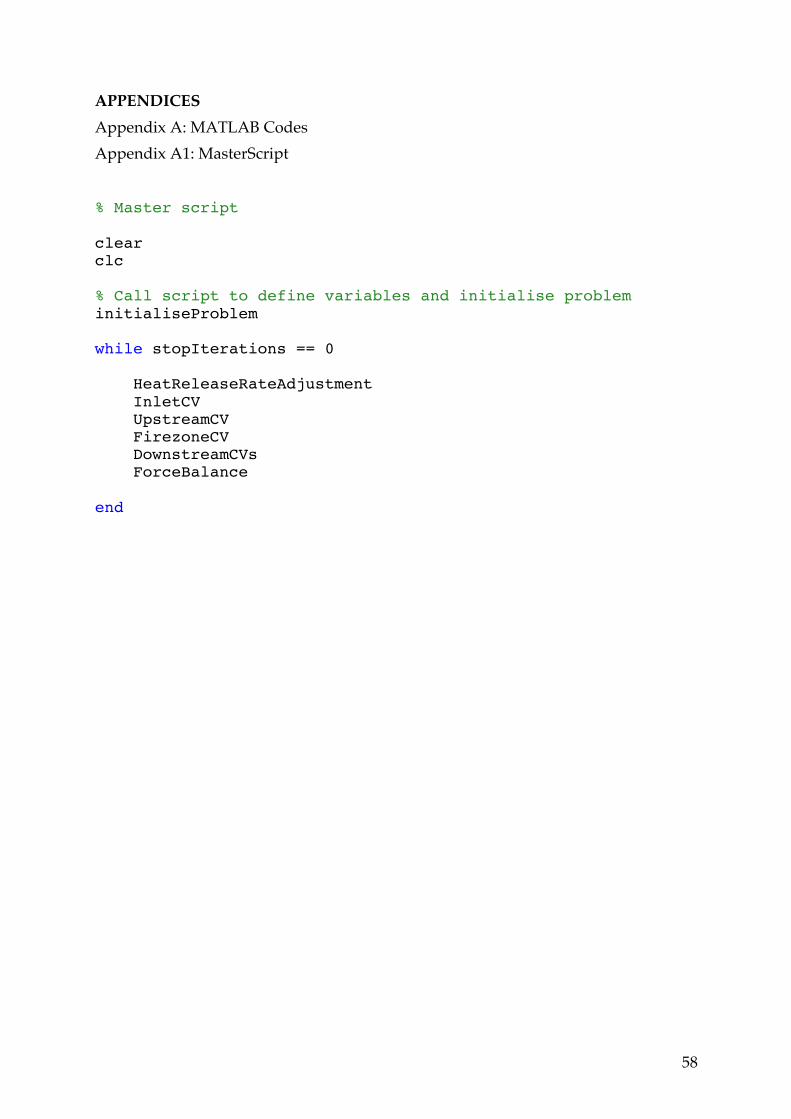
58

APPENDICES Appendix A: MATLAB Codes Appendix A1: MasterScript % Master script clear clc % Call script to define variables and initialise problem initialiseProblem while stopIterations == 0 HeatReleaseRateAdjustment InletCV UpstreamCV FirezoneCV DownstreamCVs ForceBalance end

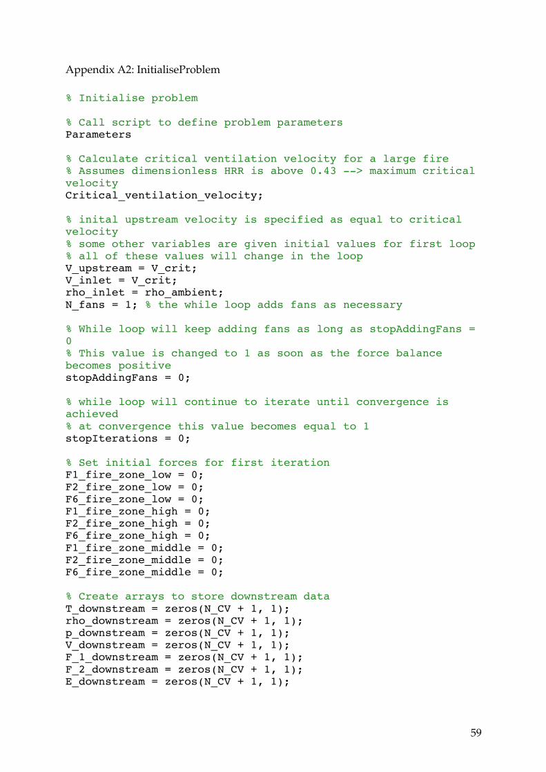
59

Appendix A2: InitialiseProblem

% Initialise problem % Call script to define problem parameters Parameters % Calculate critical ventilation velocity for a large fire % Assumes dimensionless HRR is above 0.43 --> maximum critical velocity Critical_ventilation_velocity; % inital upstream velocity is specified as equal to critical velocity % some other variables are given initial values for first loop % all of these values will change in the loop V_upstream = V_crit; V_inlet = V_crit; rho_inlet = rho_ambient; N_fans = 1; % the while loop adds fans as necessary % While loop will keep adding fans as long as stopAddingFans = 0 % This value is changed to 1 as soon as the force balance becomes positive stopAddingFans = 0; % while loop will continue to iterate until convergence is achieved % at convergence this value becomes equal to 1 stopIterations = 0; % Set initial forces for first iteration F1_fire_zone_low = 0; F2_fire_zone_low = 0; F6_fire_zone_low = 0; F1_fire_zone_high = 0; F2_fire_zone_high = 0; F6_fire_zone_high = 0; F1_fire_zone_middle = 0; F2_fire_zone_middle = 0; F6_fire_zone_middle = 0; % Create arrays to store downstream data T_downstream = zeros(N_CV + 1, 1); rho_downstream = zeros(N_CV + 1, 1); p_downstream = zeros(N_CV + 1, 1); V_downstream = zeros(N_CV + 1, 1); F_1_downstream = zeros(N_CV + 1, 1); F_2_downstream = zeros(N_CV + 1, 1); E_downstream = zeros(N_CV + 1, 1);

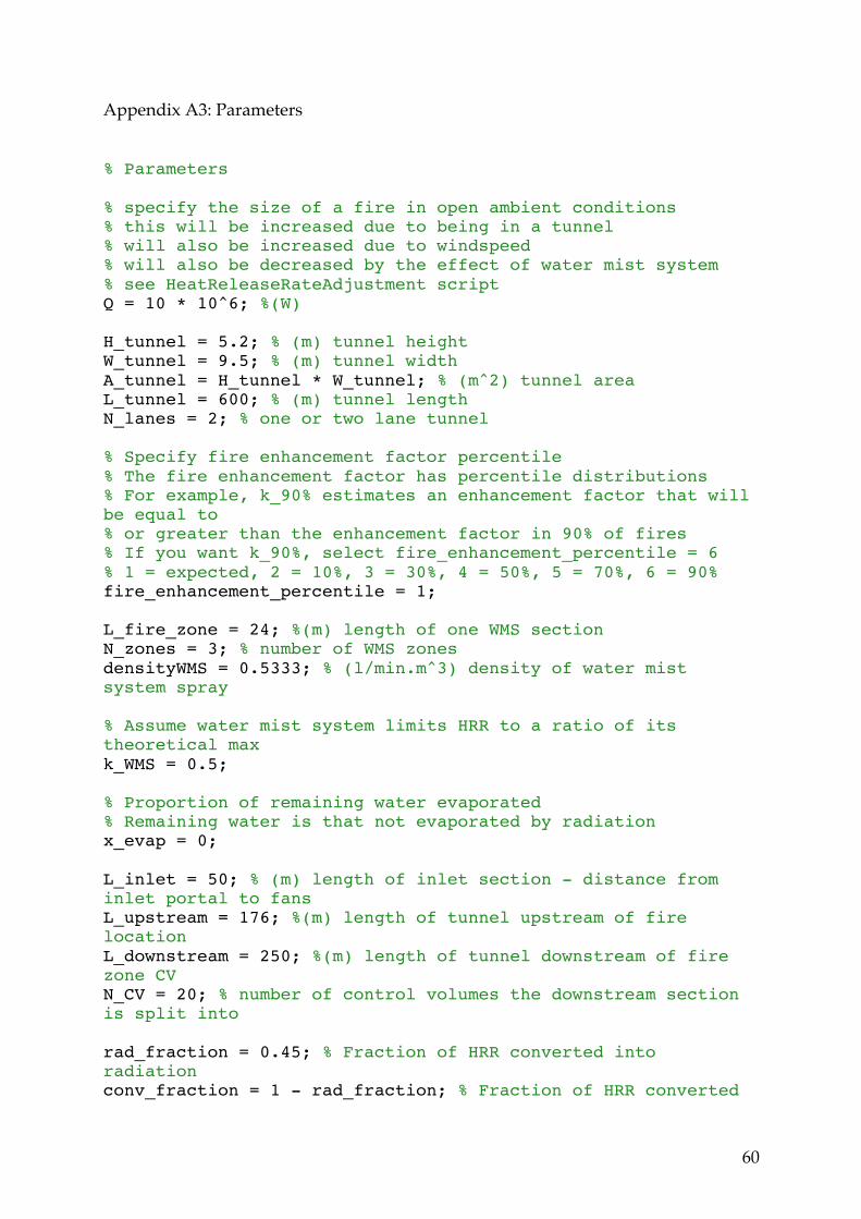
60

Appendix A3: Parameters % Parameters % specify the size of a fire in open ambient conditions % this will be increased due to being in a tunnel % will also be increased due to windspeed % will also be decreased by the effect of water mist system % see HeatReleaseRateAdjustment script Q = 10 * 10^6; %(W) H_tunnel = 5.2; % (m) tunnel height W_tunnel = 9.5; % (m) tunnel width A_tunnel = H_tunnel * W_tunnel; % (m^2) tunnel area L_tunnel = 600; % (m) tunnel length N_lanes = 2; % one or two lane tunnel % Specify fire enhancement factor percentile % The fire enhancement factor has percentile distributions % For example, k_90% estimates an enhancement factor that will be equal to % or greater than the enhancement factor in 90% of fires % If you want k_90%, select fire_enhancement_percentile = 6 % 1 = expected, 2 = 10%, 3 = 30%, 4 = 50%, 5 = 70%, 6 = 90% fire_enhancement_percentile = 1; L_fire_zone = 24; %(m) length of one WMS section N_zones = 3; % number of WMS zones densityWMS = 0.5333; % (l/min.m^3) density of water mist system spray % Assume water mist system limits HRR to a ratio of its theoretical max k_WMS = 0.5; % Proportion of remaining water evaporated % Remaining water is that not evaporated by radiation x_evap = 0; L_inlet = 50; % (m) length of inlet section - distance from inlet portal to fans L_upstream = 176; %(m) length of tunnel upstream of fire location L_downstream = 250; %(m) length of tunnel downstream of fire zone CV N_CV = 20; % number of control volumes the downstream section is split into rad_fraction = 0.45; % Fraction of HRR converted into radiation conv_fraction = 1 - rad_fraction; % Fraction of HRR converted

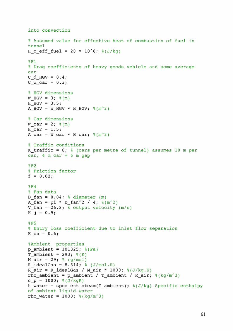
61

into convection % Assumed value for effective heat of combustion of fuel in tunnel H_c_eff_fuel = 20 * 10^6; %(J/kg) %F1 % Drag coefficients of heavy goods vehicle and some average car C_d_HGV = 0.4; C_d_car = 0.3; % HGV dimensions W_HGV = 3; %(m) H_HGV = 3.5; A_HGV = W_HGV * H_HGV; %(m^2) % Car dimensions W_car = 2; %(m) H_car = 1.5; A_car = W_car * H_car; %(m^2) % Traffic conditions K_traffic = 0; % (cars per metre of tunnel) assumes 10 m per car, 4 m car + 6 m gap %F2 % Friction factor f = 0.02; %F4 % Fan data D_fan = 0.84; % diameter (m) A_fan = pi * D_fan^2 / 4; %(m^2) V_fan = 26.2; % output velocity (m/s) K_j = 0.9; %F5 % Entry loss coefficient due to inlet flow separation K_en = 0.6; %Ambient properties p_ambient = 101325; %(Pa) T_ambient = 293; %(K) M_air = 29; % (g/mol) R_idealGas = 8.314; % (J/mol.K) R_air = R_idealGas / M_air * 1000; %(J/kg.K) rho_ambient = p_ambient / T_ambient / R_air; %(kg/m^3) c_p = 1000; %(J/kgK) h_water = spec_ent_steam(T_ambient); %(J/kg) Specific enthalpy of ambient liquid water rho_water = 1000; %(kg/m^3)

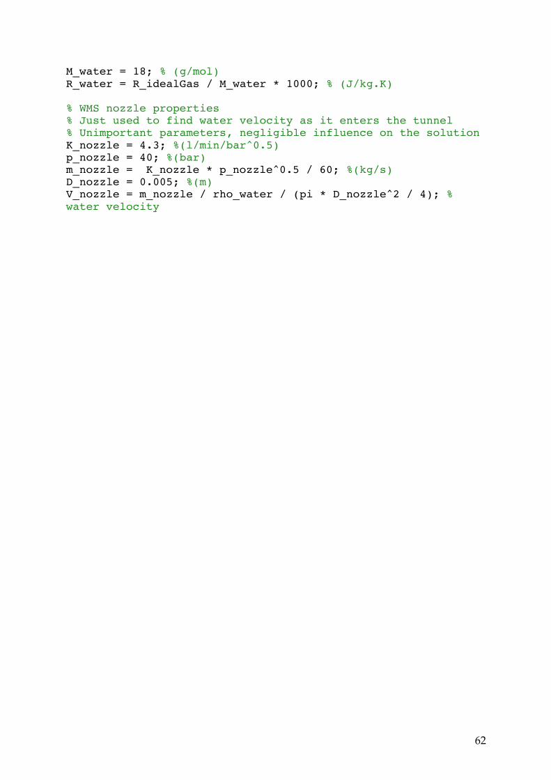
62

M_water = 18; % (g/mol) R_water = R_idealGas / M_water * 1000; % (J/kg.K) % WMS nozzle properties % Just used to find water velocity as it enters the tunnel % Unimportant parameters, negligible influence on the solution K_nozzle = 4.3; %(l/min/bar^0.5) p_nozzle = 40; %(bar) m_nozzle = K_nozzle * p_nozzle^0.5 / 60; %(kg/s) D_nozzle = 0.005; %(m) V_nozzle = m_nozzle / rho_water / (pi * D_nozzle^2 / 4); % water velocity

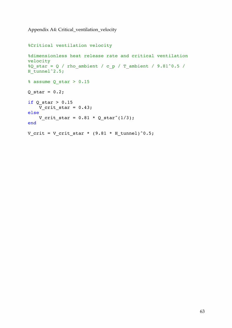
63

Appendix A4: Critical_ventilation_velocity %Critical ventilation velocity %dimensionless heat release rate and critical ventilation velocity %Q_star = Q / rho_ambient / c_p / T_ambient / 9.81^0.5 / H_tunnel^2.5; % assume Q_star > 0.15 Q_star = 0.2; if Q_star > 0.15 V_crit_star = 0.43; else V_crit_star = 0.81 * Q_star^(1/3); end V_crit = V_crit_star * (9.81 * H_tunnel)^0.5;

64

Appendix A5: HeatReleaseRateAdjustment % Heat Release Rate Adjustment % Find enhancement factor due to being in an enclosure if W_HGV / W_tunnel <= 0.5 psi = 24 * (W_HGV / W_tunnel)^3 + 1; else 'Ratio W_HGV / W_tunnel is too big' 'Tunnel enhancement factor psi is inapplicable' end Q_natural_ventilation = psi * Q; % Find ventilation velocity enhancement factor if N_lanes == 1 load('oneLane_k_factors.mat'); if fire_enhancement_percentile == 1 V_values = oneLanekfactors(:,1); enhancement_values = oneLanekfactors(:,2); elseif fire_enhancement_percentile == 2 V_values = oneLanekfactors(:,3); enhancement_values = oneLanekfactors(:,4); elseif fire_enhancement_percentile == 3 V_values = oneLanekfactors(:,5); enhancement_values = oneLanekfactors(:,6); elseif fire_enhancement_percentile == 4 V_values = oneLanekfactors(:,7); enhancement_values = oneLanekfactors(:,8); elseif fire_enhancement_percentile == 5 V_values = oneLanekfactors(:,9); enhancement_values = oneLanekfactors(:,10); elseif fire_enhancement_percentile == 6 V_values = oneLanekfactors(:,11); enhancement_values = oneLanekfactors(:,12); end

65

elseif N_lanes == 2 load('twoLane_k_factors.mat'); if fire_enhancement_percentile == 1 V_values = twoLanekfactors(:,1); enhancement_values = twoLanekfactors(:,2); elseif fire_enhancement_percentile == 2 V_values = twoLanekfactors(:,3); enhancement_values = twoLanekfactors(:,4); elseif fire_enhancement_percentile == 3 V_values = twoLanekfactors(:,5); enhancement_values = twoLanekfactors(:,6); elseif fire_enhancement_percentile == 4 V_values = twoLanekfactors(:,7); enhancement_values = twoLanekfactors(:,8); elseif fire_enhancement_percentile == 5 V_values = twoLanekfactors(:,9); enhancement_values = twoLanekfactors(:,10); elseif fire_enhancement_percentile == 6 V_values = twoLanekfactors(:,11); enhancement_values = twoLanekfactors(:,12); end end k_factor = interpolateCustom(V_values, enhancement_values, V_upstream); Q_ventilated = Q_natural_ventilation * k_factor; % Updated heat release rate Q_adjusted = Q_ventilated * k_WMS;

66

Appendix A6: interpolateCustom function k_factor = interpolateCustom(V_values, enhancement_values, V_upstream) loopBreaker = 0; for index = 1 : length(V_values) if V_values(index, 1) > V_upstream && loopBreaker == 0 k_factor = (V_upstream - V_values(index - 1, 1)) / (V_values(index, 1) - V_values(index - 1, 1)) * (enhancement_values(index, 1) - enhancement_values(index - 1, 1)) + enhancement_values(index - 1, 1); loopBreaker = 1; end end

67

Appendix A7: InletCV % Inlet CV T_inlet = T_ambient; rho_inlet = rho_ambient; m_air = rho_inlet * A_tunnel * V_inlet; N_cars_inlet = K_traffic * L_inlet; F1_inlet = -0.5 * rho_inlet * C_d_car * V_inlet^2 * A_car * N_cars_inlet; D_h = (2 * H_tunnel * W_tunnel)/(H_tunnel + W_tunnel); F2_inlet = -0.5 * f * rho_inlet * L_inlet / D_h * A_tunnel * V_inlet^2; F5 = -0.5 * K_en * rho_inlet * A_tunnel * V_inlet^2; p_inlet_portal = p_ambient - 0.5 * rho_inlet * V_inlet^2; p_losses_inlet = (F1_inlet + F2_inlet + F5) / A_tunnel; p_inlet = p_inlet_portal + p_losses_inlet;

68

Appendix A8: UpstreamCV % Upstream CV V_upstream = V_inlet; T_upstream = T_ambient; rho_upstream = rho_ambient; N_cars_upstream = K_traffic * L_upstream; F1_upstream = -0.5 * rho_upstream * C_d_car * V_upstream^2 * A_car * N_cars_upstream; F2_upstream = -0.5 * f * rho_upstream * L_upstream / D_h * A_tunnel * V_upstream^2; F4 = N_fans * rho_upstream * A_fan * V_fan * (V_fan - V_upstream) * K_j; p_fans = F4 / A_tunnel; p_losses_upstream = (F1_upstream + F2_upstream) / A_tunnel; p_upstream = p_inlet + p_fans + p_losses_upstream;

69

Appendix A9: FirezoneCV % Fire zone CV A_surface_fire_zone = 2 * L_fire_zone * (H_tunnel + W_tunnel); %(m^2) h_upstream = spec_ent_air(T_upstream); m_water = densityWMS * N_zones * L_fire_zone * W_tunnel * H_tunnel / 60; E_water = m_water * (h_water + V_nozzle^2/2 + 9.81 * H_tunnel); E_upstream = m_air * (h_upstream + V_upstream^2/2 + 9.81 * H_tunnel/2); eb_ConvergenceError = 0.0001; eb_Error = 1; T_fire_zone_low = 273; T_fire_zone_high = 2250; m_fuel = Q_adjusted / H_c_eff_fuel; m_steam_rad = rad_fraction * Q_adjusted / (spec_ent_steam(373) - h_water); m_water_lost = m_water - m_steam_rad; m_steam_conv = x_evap * m_water_lost; m_water_lost = (1 - x_evap) * m_water_lost; m_steam = m_steam_rad + m_steam_conv; if m_steam >= m_water m_steam = m_water; end m_downstream = m_air + m_fuel + m_steam; R_mix = m_air / (m_air + m_steam) * R_air + m_steam / (m_air + m_steam) * R_water; while eb_Error > eb_ConvergenceError % Low if T_fire_zone_low < 373 T_steam_low = 373; elseif T_fire_zone_low >= 373

70

T_steam_low = T_fire_zone_low; end T_water_lost_low = T_fire_zone_low; p_fire_zone_low = p_upstream + (F1_fire_zone_low + F2_fire_zone_low + F6_fire_zone_low) / A_tunnel; rho_fire_zone_low = p_fire_zone_low / R_mix / T_fire_zone_low; V_fire_zone_low = m_downstream / rho_fire_zone_low / A_tunnel; h_fire_zone_low_air = spec_ent_air(T_fire_zone_low); h_fire_zone_low_steam = spec_ent_steam(T_steam_low); h_fire_zone_low = (m_air + m_fuel) / m_downstream * h_fire_zone_low_air + m_steam / m_downstream * h_fire_zone_low_steam; h_water_lost_low = min(spec_ent_steam(T_water_lost_low), 419140); F1_fire_zone_low = rho_fire_zone_low/2 * C_d_HGV * (-V_fire_zone_low) * V_fire_zone_low * A_HGV; F2_fire_zone_low = -1 * f * rho_fire_zone_low / 2 * L_fire_zone / D_h * A_tunnel * V_fire_zone_low * abs(V_fire_zone_low); F6_fire_zone_low_air = m_air * (V_upstream - V_fire_zone_low); F6_fire_zone_low_steam = m_steam * (0 - V_fire_zone_low); F6_fire_zone_low_water = m_water_lost * (0 - V_fire_zone_low); F6_fire_zone_low = F6_fire_zone_low_air + F6_fire_zone_low_steam + F6_fire_zone_low_water; Q_loss_fire_zone_low = heat_losses(T_fire_zone_low, V_fire_zone_low, D_h, f, A_surface_fire_zone); W_fire_zone = V_fire_zone_low * (F1_fire_zone_low + F2_fire_zone_low + F6_fire_zone_low); E_fire_zone_low = m_downstream * (h_fire_zone_low + V_fire_zone_low^2/2 + 9.81 * H_tunnel/2); E_water_lost_low = m_water_lost * (h_water_lost_low + V_fire_zone_low^2/2); bal_low = Q_adjusted - Q_loss_fire_zone_low - W_fire_zone + E_upstream + E_water - E_fire_zone_low - E_water_lost_low; % High if T_fire_zone_high < 373 T_steam_high = 373;

71

elseif T_fire_zone_high >= 373 T_steam_high = T_fire_zone_high; end T_water_lost_high = T_fire_zone_high; p_fire_zone_high = p_upstream + (F1_fire_zone_high + F2_fire_zone_high + F6_fire_zone_high) / A_tunnel; rho_fire_zone_high = p_fire_zone_high / R_mix / T_fire_zone_high; V_fire_zone_high = m_downstream / rho_fire_zone_high / A_tunnel; h_fire_zone_high_air = spec_ent_air(T_fire_zone_high); h_fire_zone_high_steam = spec_ent_steam(T_steam_high); h_fire_zone_high = (m_air + m_fuel) / m_downstream * h_fire_zone_high_air + m_steam / m_downstream * h_fire_zone_high_steam; h_water_lost_high = min(spec_ent_steam(T_water_lost_high), 419140); F1_fire_zone_high = rho_fire_zone_high/2 * C_d_HGV * (-V_fire_zone_high) * V_fire_zone_high * A_HGV; F2_fire_zone_high = -1 * f * rho_fire_zone_high / 2 * L_fire_zone / D_h * A_tunnel * V_fire_zone_high * abs(V_fire_zone_high); F6_fire_zone_high_air = m_air * (V_upstream - V_fire_zone_high); F6_fire_zone_high_steam = m_steam * (0 - V_fire_zone_high); F6_fire_zone_high_water = m_water_lost * (0 - V_fire_zone_high); F6_fire_zone_high = F6_fire_zone_high_air + F6_fire_zone_high_steam + F6_fire_zone_high_water; Q_loss_fire_zone_high = heat_losses(T_fire_zone_high, V_fire_zone_high, D_h, f, A_surface_fire_zone); W_fire_zone = V_fire_zone_high * (F1_fire_zone_high + F2_fire_zone_high + F6_fire_zone_high); E_fire_zone_high = m_downstream * (h_fire_zone_high + V_fire_zone_high^2/2 + 9.81 * H_tunnel/2); E_water_lost_high = m_water_lost * (h_water_lost_high + V_fire_zone_high^2/2); bal_high = Q_adjusted - Q_loss_fire_zone_high - W_fire_zone + E_upstream + E_water - E_fire_zone_high - E_water_lost_high; %Middle

72

T_fire_zone_middle = (T_fire_zone_high + T_fire_zone_low) / 2; if T_fire_zone_middle < 373 T_steam_middle = 373; elseif T_fire_zone_middle >= 373 T_steam_middle = T_fire_zone_middle; end T_water_lost_middle = T_fire_zone_middle; p_fire_zone_middle = p_upstream + (F1_fire_zone_middle + F2_fire_zone_middle + F6_fire_zone_middle) / A_tunnel; rho_fire_zone_middle = p_fire_zone_middle / R_mix / T_fire_zone_middle; V_fire_zone_middle = m_downstream / rho_fire_zone_middle / A_tunnel; h_fire_zone_middle_air = spec_ent_air(T_fire_zone_middle); h_fire_zone_middle_steam = spec_ent_steam(T_steam_middle); h_fire_zone_middle = (m_air + m_fuel) / m_downstream * h_fire_zone_middle_air + m_steam / m_downstream * h_fire_zone_middle_steam; h_water_lost_middle = min(spec_ent_steam(T_water_lost_middle), 419140); F1_fire_zone_middle = rho_fire_zone_middle/2 * C_d_HGV * (-V_fire_zone_middle) * V_fire_zone_middle * A_HGV; F2_fire_zone_middle = -1 * f * rho_fire_zone_middle / 2 * L_fire_zone / D_h * A_tunnel * V_fire_zone_middle * abs(V_fire_zone_middle); F6_fire_zone_middle_air = m_air * (V_upstream - V_fire_zone_middle); F6_fire_zone_middle_steam = m_steam * (0 - V_fire_zone_middle); F6_fire_zone_middle_water = m_water_lost * (0 - V_fire_zone_middle); F6_fire_zone_middle = F6_fire_zone_middle_air + F6_fire_zone_middle_steam + F6_fire_zone_middle_water; Q_loss_fire_zone_middle = heat_losses(T_fire_zone_middle, V_fire_zone_middle, D_h, f, A_surface_fire_zone); W_fire_zone = V_fire_zone_middle * (F1_fire_zone_middle + F2_fire_zone_middle + F6_fire_zone_middle); E_fire_zone_middle = m_downstream * (h_fire_zone_middle + V_fire_zone_middle^2/2 + 9.81 * H_tunnel/2); E_water_lost_middle = m_water_lost * (h_water_lost_middle + V_fire_zone_middle^2/2);

73

bal_middle = Q_adjusted - Q_loss_fire_zone_middle - W_fire_zone + E_upstream + E_water - E_fire_zone_middle - E_water_lost_middle; if bal_low * bal_middle < 0 T_fire_zone_high = T_fire_zone_middle; elseif bal_high * bal_middle < 0 T_fire_zone_low = T_fire_zone_middle; else 'temperature convergence error_fire_zone' break end eb_Error = abs((T_fire_zone_high - T_fire_zone_low) / T_fire_zone_low); end % Values of temp, density and velocity in fire zone T_fire_zone = T_fire_zone_middle; % (K) p_fire_zone = p_fire_zone_middle; rho_fire_zone = rho_fire_zone_middle; V_fire_zone = V_fire_zone_middle; F1_fire_zone = F1_fire_zone_middle; F2_fire_zone = F2_fire_zone_middle; F6 = F6_fire_zone_middle; % Put the above values into arrays % These arrays will give the distribution of each parameter throughout the % downstream section of the tunnel T_downstream(1, 1) = T_fire_zone; rho_downstream(1, 1) = rho_fire_zone; V_downstream(1, 1) = V_fire_zone; p_downstream(1, 1) = p_fire_zone; F_1_downstream(1, 1) = F1_fire_zone; F_2_downstream(1, 1) = F2_fire_zone; E_downstream(1, 1) = E_fire_zone_middle; Q_losses(1, 1) = Q_loss_fire_zone_middle;

74

Appendix A10: heat_losses % Heat losses function function Q_losses = heat_losses(T_gas, V_gas, D_h, f, A_surface_CV) % Load air data for kinematic viscosity, Pr, thermal conductivity and % thermal diffusivity load('flow_data_air.mat'); % Interpolate for kinematic viscosity of air T_values = flowdataair(:,1); visc_kin_values = flowdataair(:,2); visc_kin = interp1(T_values, visc_kin_values, T_gas); % Interpolate for Prandtl number of air Pr_values = flowdataair(:,3); Pr = interp1(T_values, Pr_values, T_gas); % Interpolate for thermal conductivity of air k_values = flowdataair(:,4); k_air = interp1(T_values, k_values, T_gas); % Find Reynolds number Re = V_gas * D_h / visc_kin; % If statement to find which turbulence regime to use % Find Nusselt number accordingly if Re > 10000 % turbulent Nu = 0.125 * f * Re * Pr^(1/3); elseif Re <= 10000 % laminar Nu = 3; end % Find convective coefficient h = Nu * k_air / D_h; % Set convergence parameters for surface temperature surfaceError = 1; surfaceConvergence = 0.01; % Set initial time value and time step t_surface = 0; delta_t_surface = 60; % seconds

75

% Set ambient tunnel wall surface temperature T_surface_ambient = 293; % K % Define concrete properties alpha_conc = 0.0000005; % m2/s k_conc = 1; % W/mK while surfaceError > surfaceConvergence % Calculate surface temperature at timestep i T_surface = T_surface_ambient + (T_gas - T_surface_ambient) * (1 - exp(alpha_conc * t_surface * h^2 / k_conc^2) * erfc(sqrt(alpha_conc * t_surface) * h / k_conc)); % Increase time to timestep i+1 t_surface = t_surface + delta_t_surface; % Calculate surface temperature at timestep i+1 T_surface_new = T_surface_ambient + (T_gas - T_surface_ambient) * (1 - exp(alpha_conc * t_surface * h^2 / k_conc^2) * erfc(sqrt(alpha_conc * t_surface) * h / k_conc)); % Check if surface temperature has converged surfaceError = abs(T_surface / T_surface_new - 1); end Q_losses = h * A_surface_CV * (T_gas - T_surface_new); end

76

Appendix A11: spec_ent_air function h=spec_ent_air(T) load('thermo_data_air.mat'); T_values = thermodataair(:,1); h_values = thermodataair(:,2); h = interp1(T_values, h_values, T); end

77

Appendix A12: spec_ent_steam function h=spec_ent_steam(T) load('thermo_data_steam.mat'); T_values = thermodatawaterandsteam(:,1); h_values = thermodatawaterandsteam(:,2); h = interp1(T_values, h_values, T); end

78

Appendix A13: DownstreamCVs % Downstream energy balances L_CV = L_downstream / N_CV; A_surface_CV = 2 * L_CV * (H_tunnel + W_tunnel); %(m^2) N_cars_downstream = L_downstream * K_traffic; eb_ConvergenceError = 0.0001; eb_Error = 1; for iii = 1 : N_CV p_previous_CV = p_downstream(iii, 1); T_CV_low = 273; T_CV_high = 2250; E_previous_CV = E_downstream(iii, 1); eb_Error = 1; F1_CV_low = 0; F2_CV_low = 0; F1_CV_high = 0; F2_CV_high = 0; F1_CV_middle = 0; F2_CV_middle = 0; while eb_Error > eb_ConvergenceError % Low if T_CV_low < 373 T_steam_low = 373; else T_steam_low = T_CV_low; end p_CV_low = p_previous_CV + (F1_CV_low + F2_CV_low) / A_tunnel; rho_CV_low = p_CV_low / R_mix / T_CV_low; V_CV_low = m_downstream / rho_CV_low / A_tunnel; h_CV_low_air = spec_ent_air(T_CV_low); h_CV_low_steam = spec_ent_steam(T_steam_low); h_CV_low = (m_air + m_fuel) / m_downstream *

79

h_CV_low_air + m_steam / m_downstream * h_CV_low_steam; F1_CV_low = -0.5 * rho_CV_low * C_d_car * V_CV_low^2 * A_car * N_cars_downstream / N_CV; F2_CV_low = -0.5 * f * rho_CV_low * L_CV / D_h * A_tunnel * V_CV_low * abs(V_CV_low); Q_loss_low_CV = heat_losses(T_CV_low, V_CV_low, D_h, f, A_surface_CV); W_CV_low = V_CV_low * (F1_CV_low + F2_CV_low); E_CV_low = m_downstream * (h_CV_low + V_CV_low^2/2 + 9.81 * H_tunnel/2); bal_low = -Q_loss_low_CV - W_CV_low + E_previous_CV - E_CV_low; % High if T_CV_high < 373 T_steam_high = 373; else T_steam_high = T_CV_high; end p_CV_high = p_previous_CV + (F1_CV_high + F2_CV_high) / A_tunnel; rho_CV_high = p_CV_high / R_mix / T_CV_high; V_CV_high = m_downstream / rho_CV_high / A_tunnel; h_CV_high_air = spec_ent_air(T_CV_high); h_CV_high_steam = spec_ent_steam(T_steam_high); h_CV_high = (m_air + m_fuel) / m_downstream * h_CV_high_air + m_steam / m_downstream * h_CV_high_steam; F1_CV_high = -0.5 * rho_CV_high * C_d_car * V_CV_high^2 * A_car * N_cars_downstream / N_CV; F2_CV_high = -0.5 * f * rho_CV_high * L_CV / D_h * A_tunnel * V_CV_high^2; Q_loss_high_CV = heat_losses(T_CV_high, V_CV_high, D_h, f, A_surface_CV); W_CV_high = V_CV_high * (F1_CV_high + F2_CV_high); E_CV_high = m_downstream * (h_CV_high + V_CV_high^2/2 + 9.81 * H_tunnel/2); bal_high = -Q_loss_high_CV - W_CV_high + E_previous_CV - E_CV_high;

80

% Middle T_CV_middle = (T_CV_high + T_CV_low) / 2; if T_CV_middle < 373 T_steam_middle = 373; else T_steam_middle = T_CV_middle; end p_CV_middle = p_previous_CV + (F1_CV_middle + F2_CV_middle) / A_tunnel; rho_CV_middle = p_CV_middle / R_mix / T_CV_middle; V_CV_middle = m_downstream / rho_CV_middle / A_tunnel; h_CV_middle_air = spec_ent_air(T_CV_middle); h_CV_middle_steam = spec_ent_steam(T_steam_middle); h_CV_middle = (m_air + m_fuel) / m_downstream * h_CV_middle_air + (m_steam) / m_downstream * h_CV_middle_steam; F1_CV_middle = -0.5 * rho_CV_middle * C_d_car * V_CV_middle^2 * A_car * N_cars_downstream / N_CV; F2_CV_middle = -0.5 * f * rho_CV_middle * L_CV / D_h * A_tunnel * V_CV_middle * abs(V_CV_middle); E_CV_middle = m_downstream * (h_CV_middle + V_CV_middle^2/2 + 9.81 * H_tunnel/2); W_CV_middle = V_CV_middle * (F1_CV_middle + F2_CV_middle); Q_loss_middle_CV = heat_losses(T_CV_middle, V_CV_middle, D_h, f, A_surface_CV); bal_middle = -Q_loss_middle_CV - W_CV_middle + E_previous_CV - E_CV_middle; if bal_low * bal_middle < 0 T_CV_high = T_CV_middle; elseif bal_high * bal_middle < 0 T_CV_low = T_CV_middle; else 'temperature convergence error' 'downstream energy balances' break end eb_Error = abs((T_CV_high - T_CV_low) / T_CV_low);

81

end p_CV = p_CV_middle; T_CV = T_CV_middle; rho_CV = rho_CV_middle; V_CV = V_CV_middle; T_downstream(1 + iii, 1) = T_CV; rho_downstream(1 + iii, 1) = rho_CV; V_downstream(1 + iii, 1) = V_CV; p_downstream(1 + iii, 1) = p_CV; F_1_downstream(1 + iii, 1) = F1_CV_middle; F_2_downstream(1 + iii, 1) = F2_CV_middle; E_downstream(1 + iii, 1) = E_CV_middle; Q_losses(1 + iii, 1) = Q_loss_middle_CV; end

82

Appendix A14: ForceBalance % Force balance % Vehicle drag force F1_downstream = sum(F_1_downstream(:, 1)); F1 = F1_inlet + F1_upstream + F1_downstream; % Wall friction F2_downstream = sum(F_2_downstream(:, 1)); F2 = F2_inlet + F2_upstream + F2_downstream; % Force due to pressure difference between inlet and outlet F3 = -0.5 * rho_inlet * V_inlet^2 * A_tunnel; % Force balance F_balance = F1 + F2 + F3 + F4 + F5 + F6 if stopAddingFans == 0 if F_balance < 0 N_fans = N_fans + 1; elseif F_balance > 0 stopAddingFans = 1; end end if stopAddingFans == 1 if F_balance > 50 V_inlet = V_inlet * 1.01; elseif F_balance >= 10 && F_balance <= 50 V_inlet = V_inlet * 1.001; elseif F_balance < 10 V_inlet = V_inlet * 1.0001; elseif F_balance < -10 V_inlet = V_inlet * 0.999; elseif F_balance > -10 && F_balance <= 0

83

V_inlet = V_inlet * 0.9999; end if abs(F_balance) < 1 stopIterations = 1; end end

84

Appendix B: Example input values

Parameter Value (unit) Ref. HRR in open, still, ambient conditions User defined (W) - Tunnel height User defined (m) - Tunnel width User defined (m) - Tunnel cross sectional area User defined (m2) - Tunnel length User defined (m) - Number of lanes User defined; either 1 or 2 (-) [19] Forced ventilation enhancement factor percentile

User defined; either 10%, 30%, 50%, expected, 70%, or 90% (-)

[19]

Length of water mist system zone 30 (m) [6] Number of water mist system zones User defined (-) - Water mist system mass flux density 0.5 (l/min/m3) [6] HRR reduction due to WMS 0.35 (-) [6] Proportion of water evaporating User defined (-) - Length of inlet section User defined (m) - Length of tunnel upstream of fire zone User defined (m) - Length of tunnel downstream of fire zone

User defined (m) -

Number of CVs the downstream section is divided into

User defined (-) -

Radiative fraction 0.35 (-) [12] Effective heat of combustion of fuel load in tunnel

20 × 10! (J/kg) [43]

HGV height User defined (m) - HGV width User defined (m) - HGV drag coefficient 0.4 (-) [49] Car height 1.5 (m) - Car width 2 (m) - Car drag coefficient 0.3 (-) [49] Traffic density 15 (vehicles/lane/km) [49] Tunnel wall friction factor 0.02 (-) [28] Fan diameter 0.84 (m) [50] Fan outlet velocity 26.2 (m/s) [50] Fan pressure rise coefficient 0.9 (-) [28] Tunnel flow inlet separation factor 0.6 (-) [28]

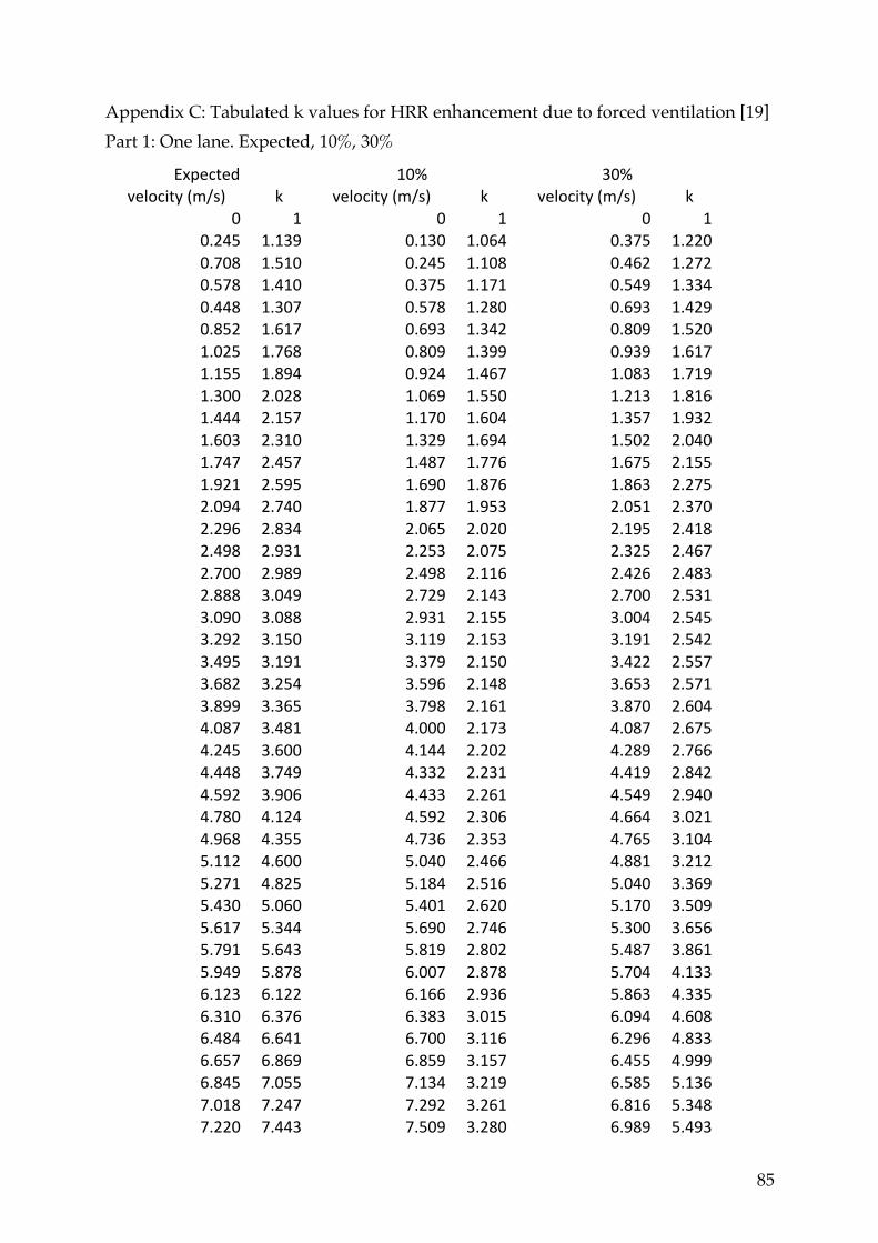
85

Appendix C: Tabulated k values for HRR enhancement due to forced ventilation [19] Part 1: One lane. Expected, 10%, 30%

Expected 10% 30%velocity(m/s) k velocity(m/s) k velocity(m/s) k

0 1 0 1 0 10.245 1.139 0.130 1.064 0.375 1.2200.708 1.510 0.245 1.108 0.462 1.2720.578 1.410 0.375 1.171 0.549 1.3340.448 1.307 0.578 1.280 0.693 1.4290.852 1.617 0.693 1.342 0.809 1.5201.025 1.768 0.809 1.399 0.939 1.6171.155 1.894 0.924 1.467 1.083 1.7191.300 2.028 1.069 1.550 1.213 1.8161.444 2.157 1.170 1.604 1.357 1.9321.603 2.310 1.329 1.694 1.502 2.0401.747 2.457 1.487 1.776 1.675 2.1551.921 2.595 1.690 1.876 1.863 2.2752.094 2.740 1.877 1.953 2.051 2.3702.296 2.834 2.065 2.020 2.195 2.4182.498 2.931 2.253 2.075 2.325 2.4672.700 2.989 2.498 2.116 2.426 2.4832.888 3.049 2.729 2.143 2.700 2.5313.090 3.088 2.931 2.155 3.004 2.5453.292 3.150 3.119 2.153 3.191 2.5423.495 3.191 3.379 2.150 3.422 2.5573.682 3.254 3.596 2.148 3.653 2.5713.899 3.365 3.798 2.161 3.870 2.6044.087 3.481 4.000 2.173 4.087 2.6754.245 3.600 4.144 2.202 4.289 2.7664.448 3.749 4.332 2.231 4.419 2.8424.592 3.906 4.433 2.261 4.549 2.9404.780 4.124 4.592 2.306 4.664 3.0214.968 4.355 4.736 2.353 4.765 3.1045.112 4.600 5.040 2.466 4.881 3.2125.271 4.825 5.184 2.516 5.040 3.3695.430 5.060 5.401 2.620 5.170 3.5095.617 5.344 5.690 2.746 5.300 3.6565.791 5.643 5.819 2.802 5.487 3.8615.949 5.878 6.007 2.878 5.704 4.1336.123 6.122 6.166 2.936 5.863 4.3356.310 6.376 6.383 3.015 6.094 4.6086.484 6.641 6.700 3.116 6.296 4.8336.657 6.869 6.859 3.157 6.455 4.9996.845 7.055 7.134 3.219 6.585 5.1367.018 7.247 7.292 3.261 6.816 5.3487.220 7.443 7.509 3.280 6.989 5.493

86

7.408 7.592 7.697 3.323 7.148 5.6047.610 7.690 7.957 3.341 7.292 5.7177.812 7.735 8.303 3.358 7.408 5.7948.000 7.781 8.606 3.376 7.552 5.8708.188 7.828 8.953 3.370 7.711 5.9478.390 7.765 9.256 3.365 7.856 6.0268.578 7.758 9.430 3.362 8.072 6.1038.780 7.696 9.661 3.358 8.260 6.1828.968 7.636 9.747 3.356 8.419 6.2209.170 7.523

8.578 6.258

9.357 7.412

8.780 6.2959.545 7.353

9.054 6.330

9.718 7.296

9.213 6.324

9.401 6.362

9.545 6.357

9.747 6.351

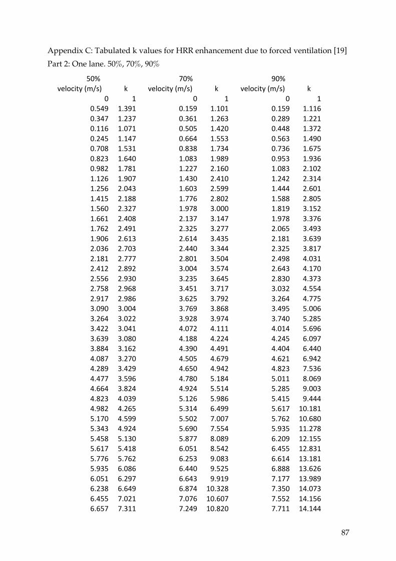
87

Appendix C: Tabulated k values for HRR enhancement due to forced ventilation [19] Part 2: One lane. 50%, 70%, 90%

50% 70% 90%velocity(m/s) k velocity(m/s) k velocity(m/s) k

0 1 0 1 0 10.549 1.391 0.159 1.101 0.159 1.1160.347 1.237 0.361 1.263 0.289 1.2210.116 1.071 0.505 1.420 0.448 1.3720.245 1.147 0.664 1.553 0.563 1.4900.708 1.531 0.838 1.734 0.736 1.6750.823 1.640 1.083 1.989 0.953 1.9360.982 1.781 1.227 2.160 1.083 2.1021.126 1.907 1.430 2.410 1.242 2.3141.256 2.043 1.603 2.599 1.444 2.6011.415 2.188 1.776 2.802 1.588 2.8051.560 2.327 1.978 3.000 1.819 3.1521.661 2.408 2.137 3.147 1.978 3.3761.762 2.491 2.325 3.277 2.065 3.4931.906 2.613 2.614 3.435 2.181 3.6392.036 2.703 2.440 3.344 2.325 3.8172.181 2.777 2.801 3.504 2.498 4.0312.412 2.892 3.004 3.574 2.643 4.1702.556 2.930 3.235 3.645 2.830 4.3732.758 2.968 3.451 3.717 3.032 4.5542.917 2.986 3.625 3.792 3.264 4.7753.090 3.004 3.769 3.868 3.495 5.0063.264 3.022 3.928 3.974 3.740 5.2853.422 3.041 4.072 4.111 4.014 5.6963.639 3.080 4.188 4.224 4.245 6.0973.884 3.162 4.390 4.491 4.404 6.4404.087 3.270 4.505 4.679 4.621 6.9424.289 3.429 4.650 4.942 4.823 7.5364.477 3.596 4.780 5.184 5.011 8.0694.664 3.824 4.924 5.514 5.285 9.0034.823 4.039 5.126 5.986 5.415 9.4444.982 4.265 5.314 6.499 5.617 10.1815.170 4.599 5.502 7.007 5.762 10.6805.343 4.924 5.690 7.554 5.935 11.2785.458 5.130 5.877 8.089 6.209 12.1555.617 5.418 6.051 8.542 6.455 12.8315.776 5.762 6.253 9.083 6.614 13.1815.935 6.086 6.440 9.525 6.888 13.6266.051 6.297 6.643 9.919 7.177 13.9896.238 6.649 6.874 10.328 7.350 14.0736.455 7.021 7.076 10.607 7.552 14.1566.657 7.311 7.249 10.820 7.711 14.144

88

6.787 7.511 7.422 10.961 7.913 14.1306.917 7.664 7.552 11.030 8.101 14.0187.134 7.925 7.971 11.160 8.404 13.7087.307 8.085 7.740 11.096 8.693 13.4067.523 8.245 8.245 11.067 9.083 12.8347.711 8.352 8.477 10.977 9.386 12.3778.029 8.514 8.693 10.814 9.661 11.9388.404 8.556 8.910 10.653 9.762 11.7688.664 8.545 9.170 10.420

8.881 8.535 9.329 10.268 9.155 8.464 9.545 10.045 9.458 8.392 9.747 9.828 9.675 8.325

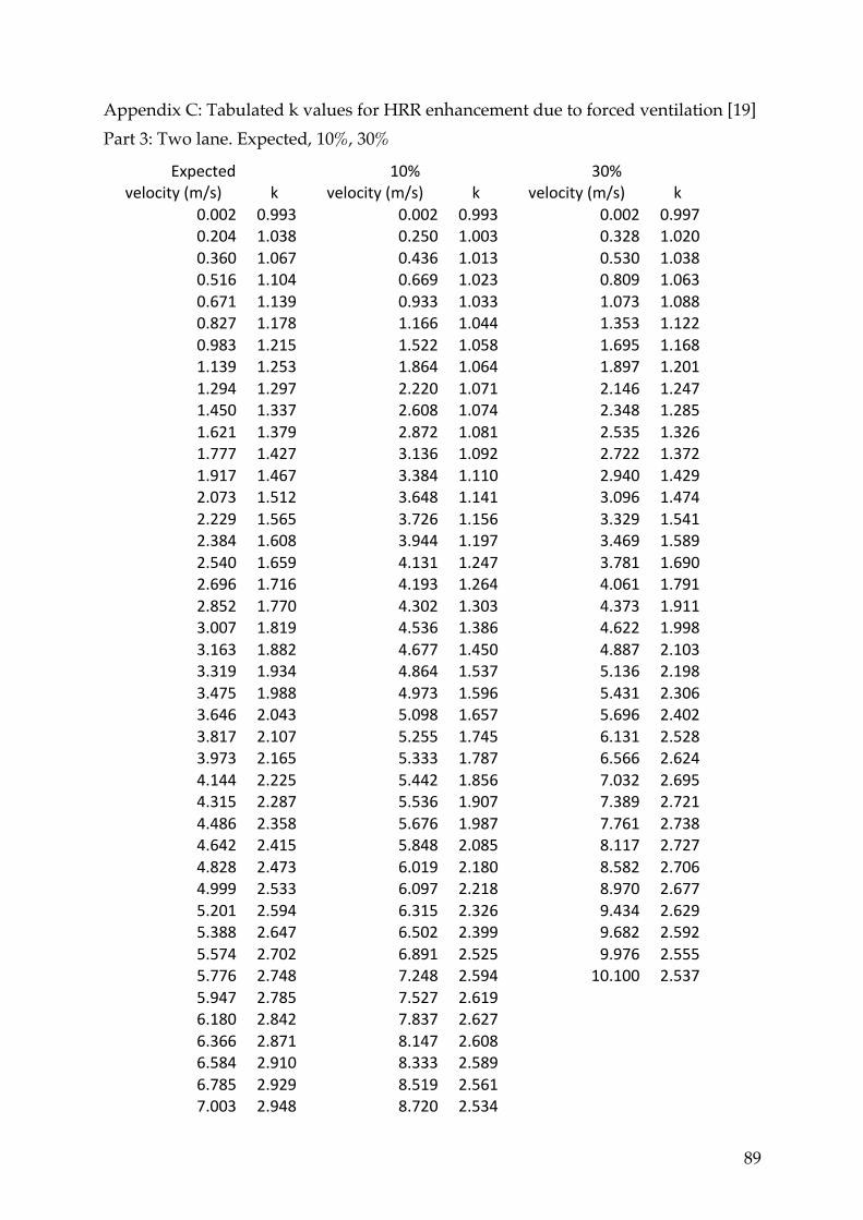
89

Appendix C: Tabulated k values for HRR enhancement due to forced ventilation [19] Part 3: Two lane. Expected, 10%, 30%

Expected 10% 30%velocity(m/s) k velocity(m/s) k velocity(m/s) k

0.002 0.993 0.002 0.993 0.002 0.9970.204 1.038 0.250 1.003 0.328 1.0200.360 1.067 0.436 1.013 0.530 1.0380.516 1.104 0.669 1.023 0.809 1.0630.671 1.139 0.933 1.033 1.073 1.0880.827 1.178 1.166 1.044 1.353 1.1220.983 1.215 1.522 1.058 1.695 1.1681.139 1.253 1.864 1.064 1.897 1.2011.294 1.297 2.220 1.071 2.146 1.2471.450 1.337 2.608 1.074 2.348 1.2851.621 1.379 2.872 1.081 2.535 1.3261.777 1.427 3.136 1.092 2.722 1.3721.917 1.467 3.384 1.110 2.940 1.4292.073 1.512 3.648 1.141 3.096 1.4742.229 1.565 3.726 1.156 3.329 1.5412.384 1.608 3.944 1.197 3.469 1.5892.540 1.659 4.131 1.247 3.781 1.6902.696 1.716 4.193 1.264 4.061 1.7912.852 1.770 4.302 1.303 4.373 1.9113.007 1.819 4.536 1.386 4.622 1.9983.163 1.882 4.677 1.450 4.887 2.1033.319 1.934 4.864 1.537 5.136 2.1983.475 1.988 4.973 1.596 5.431 2.3063.646 2.043 5.098 1.657 5.696 2.4023.817 2.107 5.255 1.745 6.131 2.5283.973 2.165 5.333 1.787 6.566 2.6244.144 2.225 5.442 1.856 7.032 2.6954.315 2.287 5.536 1.907 7.389 2.7214.486 2.358 5.676 1.987 7.761 2.7384.642 2.415 5.848 2.085 8.117 2.7274.828 2.473 6.019 2.180 8.582 2.7064.999 2.533 6.097 2.218 8.970 2.6775.201 2.594 6.315 2.326 9.434 2.6295.388 2.647 6.502 2.399 9.682 2.5925.574 2.702 6.891 2.525 9.976 2.5555.776 2.748 7.248 2.594 10.100 2.5375.947 2.785 7.527 2.619

6.180 2.842 7.837 2.627 6.366 2.871 8.147 2.608 6.584 2.910 8.333 2.589 6.785 2.929 8.519 2.561 7.003 2.948 8.720 2.534

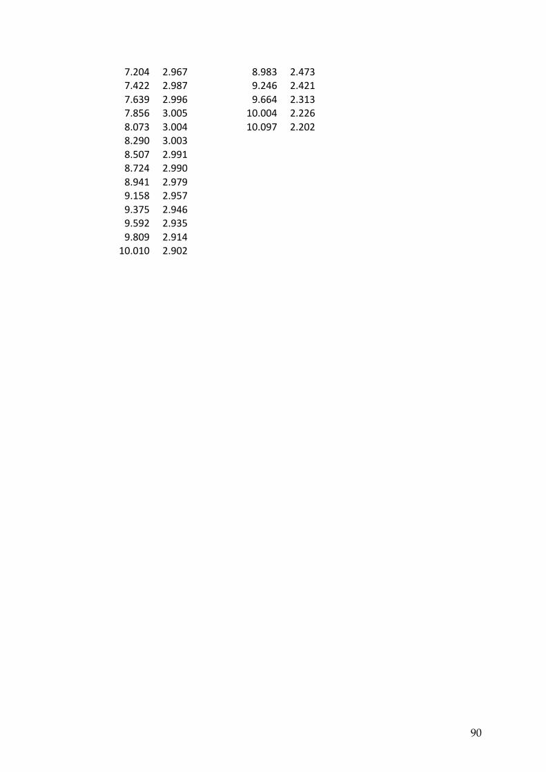
90

7.204 2.967 8.983 2.473 7.422 2.987 9.246 2.421 7.639 2.996 9.664 2.313 7.856 3.005 10.004 2.226 8.073 3.004 10.097 2.202 8.290 3.003

8.507 2.991 8.724 2.990 8.941 2.979 9.158 2.957 9.375 2.946 9.592 2.935 9.809 2.914 10.010 2.902

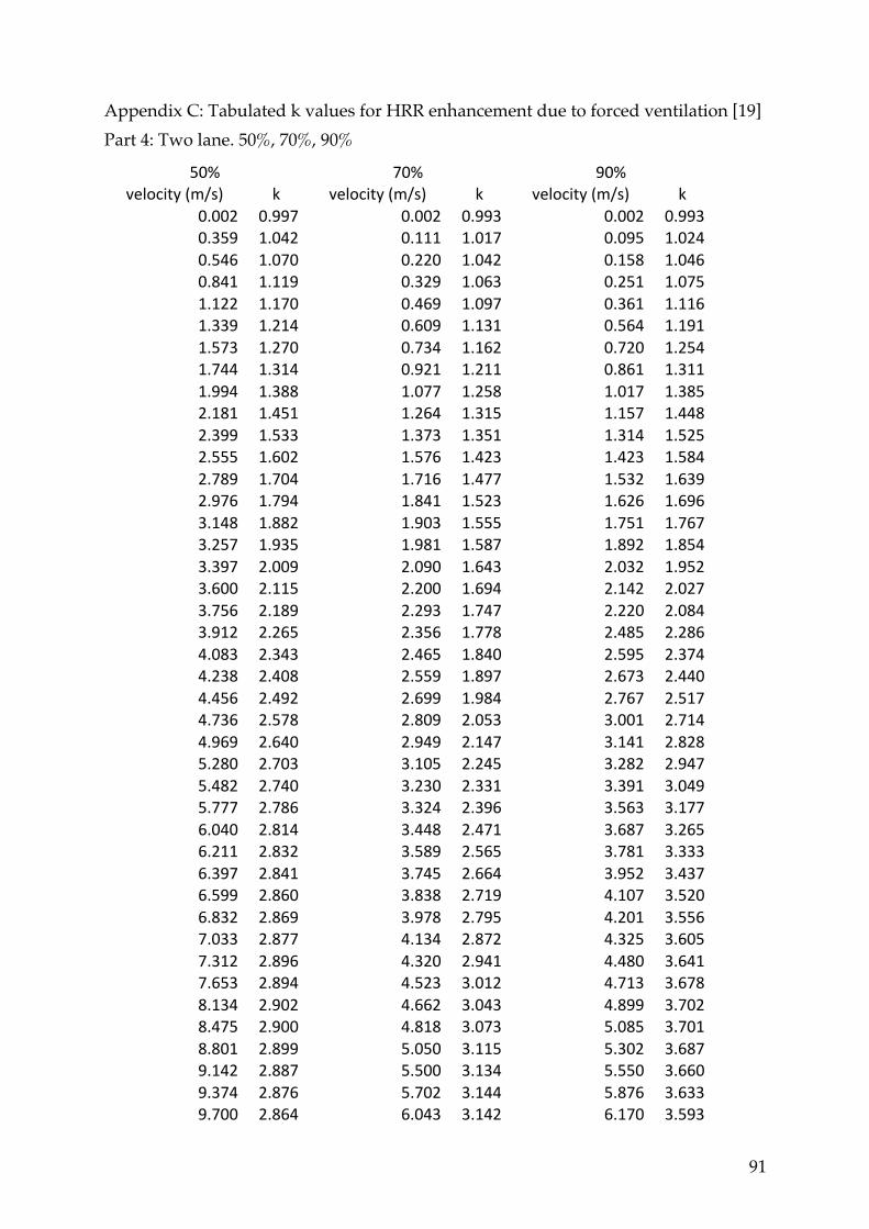
91

Appendix C: Tabulated k values for HRR enhancement due to forced ventilation [19] Part 4: Two lane. 50%, 70%, 90%

50% 70% 90%velocity(m/s) k velocity(m/s) k velocity(m/s) k

0.002 0.997 0.002 0.993 0.002 0.9930.359 1.042 0.111 1.017 0.095 1.0240.546 1.070 0.220 1.042 0.158 1.0460.841 1.119 0.329 1.063 0.251 1.0751.122 1.170 0.469 1.097 0.361 1.1161.339 1.214 0.609 1.131 0.564 1.1911.573 1.270 0.734 1.162 0.720 1.2541.744 1.314 0.921 1.211 0.861 1.3111.994 1.388 1.077 1.258 1.017 1.3852.181 1.451 1.264 1.315 1.157 1.4482.399 1.533 1.373 1.351 1.314 1.5252.555 1.602 1.576 1.423 1.423 1.5842.789 1.704 1.716 1.477 1.532 1.6392.976 1.794 1.841 1.523 1.626 1.6963.148 1.882 1.903 1.555 1.751 1.7673.257 1.935 1.981 1.587 1.892 1.8543.397 2.009 2.090 1.643 2.032 1.9523.600 2.115 2.200 1.694 2.142 2.0273.756 2.189 2.293 1.747 2.220 2.0843.912 2.265 2.356 1.778 2.485 2.2864.083 2.343 2.465 1.840 2.595 2.3744.238 2.408 2.559 1.897 2.673 2.4404.456 2.492 2.699 1.984 2.767 2.5174.736 2.578 2.809 2.053 3.001 2.7144.969 2.640 2.949 2.147 3.141 2.8285.280 2.703 3.105 2.245 3.282 2.9475.482 2.740 3.230 2.331 3.391 3.0495.777 2.786 3.324 2.396 3.563 3.1776.040 2.814 3.448 2.471 3.687 3.2656.211 2.832 3.589 2.565 3.781 3.3336.397 2.841 3.745 2.664 3.952 3.4376.599 2.860 3.838 2.719 4.107 3.5206.832 2.869 3.978 2.795 4.201 3.5567.033 2.877 4.134 2.872 4.325 3.6057.312 2.896 4.320 2.941 4.480 3.6417.653 2.894 4.523 3.012 4.713 3.6788.134 2.902 4.662 3.043 4.899 3.7028.475 2.900 4.818 3.073 5.085 3.7018.801 2.899 5.050 3.115 5.302 3.6879.142 2.887 5.500 3.134 5.550 3.6609.374 2.876 5.702 3.144 5.876 3.6339.700 2.864 6.043 3.142 6.170 3.593

92

9.948 2.853 6.291 3.141 6.309 3.58010.103 2.843 6.648 3.139 6.480 3.567

6.803 3.138 6.635 3.566

7.004 3.137 6.774 3.565

7.175 3.147 6.929 3.552

7.345 3.146 7.053 3.551

7.686 3.155 7.146 3.550

7.934 3.153 7.255 3.550

8.152 3.163 7.441 3.561

8.415 3.162 7.581 3.560

8.648 3.171 7.705 3.559

9.237 3.179 7.860 3.571

9.702 3.187 7.999 3.570

9.966 3.197 8.170 3.581

5.283 3.124 8.294 3.580

8.402 3.592

8.682 3.603

8.961 3.626

9.209 3.649

9.457 3.660

9.721 3.697

9.845 3.696

9.985 3.708

10.093 3.720

93

Appendix D: Flow data for air [45]

T(K)viscosity(m^2/s) Pr k(W/mK)

thermaldiffusivity(m^2/s)

100 1.92E-06 0.768 0.009246 2.50E-06150 4.34E-06 0.756 0.013735 5.74E-06200 7.51E-06 0.739 0.01809 1.02E-05250 1.05E-05 0.722 0.02227 1.57E-05300 1.68E-05 0.708 0.02624 2.22E-05350 2.08E-05 0.697 0.03003 2.98E-05400 2.59E-05 0.689 0.03365 3.76E-05450 3.17E-05 0.683 0.03707 4.64E-05500 3.79E-05 0.68 0.04038 5.56E-05550 4.43E-05 0.68 0.0436 6.53E-05600 5.13E-05 0.682 0.04659 7.51E-05650 5.85E-05 0.682 0.04953 8.58E-05700 6.63E-05 0.684 0.0523 9.67E-05750 7.39E-05 0.686 0.05509 0.00010774800 8.23E-05 0.689 0.05779 0.00011951850 9.08E-05 0.692 0.06028 0.00013097900 9.93E-05 0.696 0.06279 0.00014271950 0.0001082 0.699 0.06525 0.00015511000 0.0001178 0.702 0.06752 0.000167791100 0.0001386 0.704 0.0732 0.00019691200 0.0001591 0.707 0.0782 0.00022511300 0.0001821 0.705 0.0837 0.00025831400 0.0002055 0.705 0.0891 0.0002921500 0.0002291 0.705 0.0946 0.00032661600 0.0002545 0.705 0.1 0.00036241700 0.0002809 0.705 0.105 0.00039771800 0.0003081 0.704 0.111 0.00043791900 0.0003385 0.704 0.117 0.00048112000 0.000369 0.702 0.124 0.0005262100 0.0003996 0.703 0.131 0.0005682200 0.0004326 0.707 0.139 0.00061152300 0.000464 0.71 0.149 0.00065372400 0.000504 0.718 0.161 0.00070162500 0.000543 0.73 0.175 0.0007437

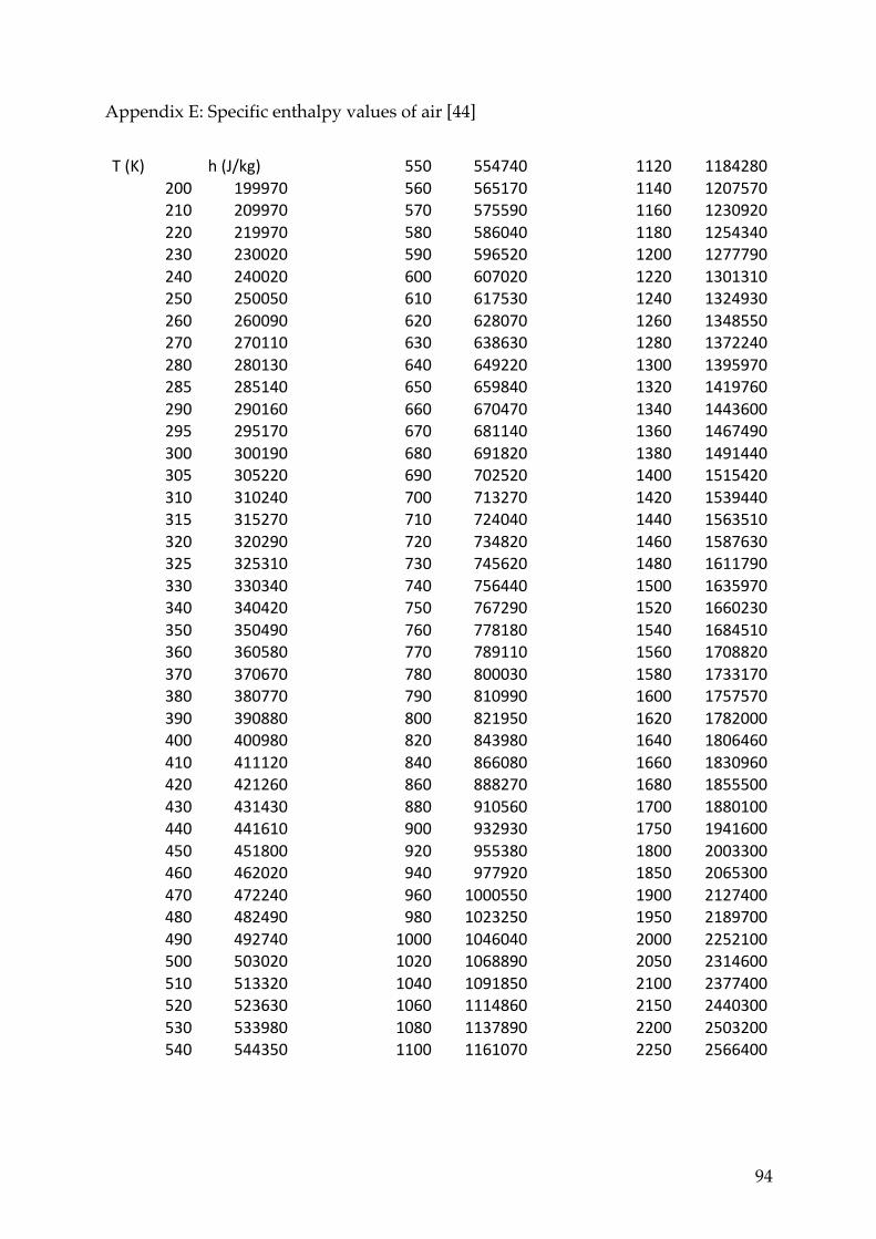
94

Appendix E: Specific enthalpy values of air [44]

T(K) h(J/kg)

200 199970210 209970220 219970230 230020240 240020250 250050260 260090270 270110280 280130285 285140290 290160295 295170300 300190305 305220310 310240315 315270320 320290325 325310330 330340340 340420350 350490360 360580370 370670380 380770390 390880400 400980410 411120420 421260430 431430440 441610450 451800460 462020470 472240480 482490490 492740500 503020510 513320520 523630530 533980540 544350

550 554740560 565170570 575590580 586040590 596520600 607020610 617530620 628070630 638630640 649220650 659840660 670470670 681140680 691820690 702520700 713270710 724040720 734820730 745620740 756440750 767290760 778180770 789110780 800030790 810990800 821950820 843980840 866080860 888270880 910560900 932930920 955380940 977920960 1000550980 10232501000 10460401020 10688901040 10918501060 11148601080 11378901100 1161070

1120 11842801140 12075701160 12309201180 12543401200 12777901220 13013101240 13249301260 13485501280 13722401300 13959701320 14197601340 14436001360 14674901380 14914401400 15154201420 15394401440 15635101460 15876301480 16117901500 16359701520 16602301540 16845101560 17088201580 17331701600 17575701620 17820001640 18064601660 18309601680 18555001700 18801001750 19416001800 20033001850 20653001900 21274001950 21897002000 22521002050 23146002100 23774002150 24403002200 25032002250 2566400

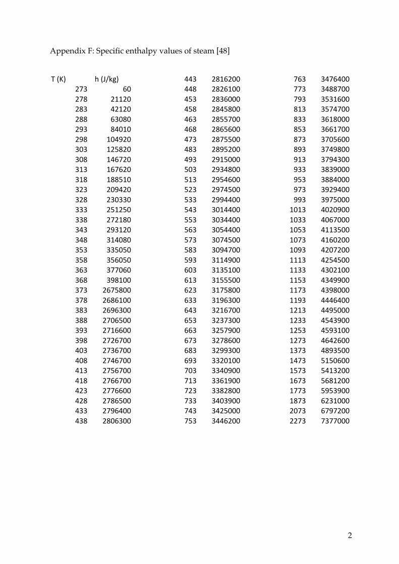
2

Appendix F: Specific enthalpy values of steam [48]

T(K) h(J/kg)273 60278 21120283 42120288 63080293 84010298 104920303 125820308 146720313 167620318 188510323 209420328 230330333 251250338 272180343 293120348 314080353 335050358 356050363 377060368 398100373 2675800378 2686100383 2696300388 2706500393 2716600398 2726700403 2736700408 2746700413 2756700418 2766700423 2776600428 2786500433 2796400438 2806300

443 2816200448 2826100453 2836000458 2845800463 2855700468 2865600473 2875500483 2895200493 2915000503 2934800513 2954600523 2974500533 2994400543 3014400553 3034400563 3054400573 3074500583 3094700593 3114900603 3135100613 3155500623 3175800633 3196300643 3216700653 3237300663 3257900673 3278600683 3299300693 3320100703 3340900713 3361900723 3382800733 3403900743 3425000753 3446200

763 3476400773 3488700793 3531600813 3574700833 3618000853 3661700873 3705600893 3749800913 3794300933 3839000953 3884000973 3929400993 3975000

1013 40209001033 40670001053 41135001073 41602001093 42072001113 42545001133 43021001153 43499001173 43980001193 44464001213 44950001233 45439001253 45931001273 46426001373 48935001473 51506001573 54132001673 56812001773 59539001873 62310002073 67972002273 7377000