The Trajectory from School to Work: A Study of Life Chances ...

City University of New York (CUNY) City University of New York (CUNY)

CUNY Academic Works CUNY Academic Works

Dissertations, Theses, and Capstone Projects CUNY Graduate Center

9-2018

The Trajectory from School to Work: A Study of Life Chances of The Trajectory from School to Work: A Study of Life Chances of

School Leavers in the United States, the United Kingdom, School Leavers in the United States, the United Kingdom,

Germany, and Sweden Germany, and Sweden

Dirk Witteveen The Graduate Center, City University of New York

How does access to this work benefit you? Let us know!

More information about this work at: https://academicworks.cuny.edu/gc_etds/2821

Discover additional works at: https://academicworks.cuny.edu

This work is made publicly available by the City University of New York (CUNY). Contact: [email protected]

https://academicworks.cuny.edu/

https://academicworks.cuny.edu/gc_etds

https://academicworks.cuny.edu/gc

http://ols.cuny.edu/academicworks/?ref=https://academicworks.cuny.edu/gc_etds/2821

https://academicworks.cuny.edu/gc_etds/2821

https://academicworks.cuny.edu/?

mailto:[email protected]

THE TRAJECTORY FROM SCHOOL TO WORK. A STUDY OF LIFE

CHANCES OF SCHOOL LEAVERS IN THE UNITED STATES, THE

UNITED KINGDOM, GERMANY, AND SWEDEN

by

DIRK WITTEVEEN

A dissertation submitted to the Graduate Faculty in Sociology in partial fulfillment of the

requirements for the degree of Doctor of Philosophy, The City University of New York

2018

ii

© 2018

DIRK WITTEVEEN

All Rights Reserved

iii

The Trajectory from School to Work. A Study of Life Chances of School Leavers in the

United States, the United Kingdom, Germany, and Sweden.

by

Dirk Witteveen

This manuscript has been read and accepted for the Graduate Faculty in

Sociology in satisfaction of the dissertation requirement for the degree of

Doctor of Philosophy.

Date Paul Attewell

Chair of Examining Committee

Date Lynn Chancer

Executive Officer

Supervisory

Committee:

Janet Gornick

Richard Alba

Mary Clare Lennon

THE CITY UNIVERSITY OF NEW YORK

iv

ABSTRACT

The Trajectory from School to Work. A Study of Life Chances of School Leavers in the

United States, the United Kingdom, Germany, and Sweden.

by

Dirk Witteveen

Advisor: Paul Attewell

The school-to-work transition is traditionally perceived as a one-time event; moving from

education to one’s first job. In response to the increased complexity within today’s relationship

between education and work, the research in this dissertation takes a different approach to the

study of inequality and stratification. It considers the life phase between these two institutions as

a trajectory – a pathway of several years wherein school careers and work careers overlap and

interact.

Given the longitudinal approach, this study starts with a comparison of patterns of school-

to-work trajectories in four distinct welfare state regimes: the United States, the United Kingdom,

Germany, and Sweden. By aligning the individual pathways of individuals between age 16

(enrolled in high school) and age 25, social sequence analysis enabled us to reveal sharp

differences in school leaving pace, school enrollment, and instability of early work careers. The

analyses suggest that the variation in selection and sorting within youth careers can be largely

explained by indicators of the different welfare state regimes. Based on comparisons of younger

and older birth cohorts there is evidence supporting convergence theory of welfare states – early

careers liberal states are becoming less volatile, while those in social-democratic states are

becoming more insecure.

v

In addition to these structural variation within the school-to-work pathway, this study

reveals how and when the state of the macro-economy affects school leaving and school reentry

behavior of different groups. In contrast to hypotheses drawn from human capital theory, high

school students in the United States are more likely to leave the educational system in times of

economic downturn. This is called a ‘discouraged student effect.’ Furthermore, among those who

have made a first transition to the labor market, lower-educated school leavers in the United States

become less likely to return to the educational system under recessionary macro conditions. This

US-specific finding suggests an ‘acquired risk aversion’ in response to economic downturn,

thereby further widening inequality of labor market chances between lower- and higher-educated

individuals. In contrast, British, Swedish, and German youths are more likely to spend more time

in full-time education in response to a recession. This is called a ‘human capital catch-up’ response.

Once youths have entered the labor market, the social sequence analyses reveal the

consequences of continued exposure to precarious positions, such as temporary work, doubling-

up jobs, and alternating between (part-time) employment and unemployment. Young people who

become stuck in such careers experience the long-term ‘scars’ of both unfavorable macro-

economic conditions and lower-paid and insecure employment. Exposure to such ‘precarious early

careers’ can be linked to substantial earnings disadvantages several years after the labor market

entry.

vi

Acknowledgements.

Upon submitting the last requirement for this degree, I look back on six fantastic years at the

CUNY Graduate Center. I thank everyone in the Sociology program for creating such a great

atmosphere. This supportive and positive environment has motivated me to spend a lot of time in

the Department to work on coursework, papers, and this dissertation. I have enjoyed it every single

day.

I would like to express my sincere gratitude to my dissertation chair and academic advisor,

Prof. Paul Attewell, whose guidance and intellectual support have been essential for my doctoral

training. I am also grateful for the opportunity to work as research assistant on several of Prof.

Attewell’s projects since the first year of my PhD studies. It allowed me to learn all kinds of skills

of academic research in an ambitious and inspiring team. The thought-provoking conversations

and discussions about research questions, data, and modeling have helped me tremendously

throughout my studies – in particular for writing my dissertation.

I thank my three other committee members for their encouragement and insightful

comments, and above all for widening my scope of sociological research. I thank Prof. Janet

Gornick for introducing me to international data-use and welfare state studies, Prof. Mary Clare

Lennon for encouraging me to get my research out in life course studies, and Prof. Alba for our

fine collaboration on the project on the second generation in the Netherlands. I could not have

wished for a more knowledgeable and supportive committee. Many thanks.

Special thanks to Rati Kashyap who has been so helpful at guiding me through the program

at difficult moments. I also thank Darren Kwong, Annette Jacoby, Brenden Beck, and David

Monaghan for helping me out with the earliest drafts of my work and the countless statistics

vii

questions, and of course for the fun times outside of school. Champions League afternoons and

Euro / World Cup summers would not have been the same without Mehdi Bezorgmehr and his

passion for soccer – thank you for sharing those great moments in the thesis room and my cubicle.

I thank all my friends and my family – my parents and my brother in particular – for their

unconditional support, love, and patience!

viii

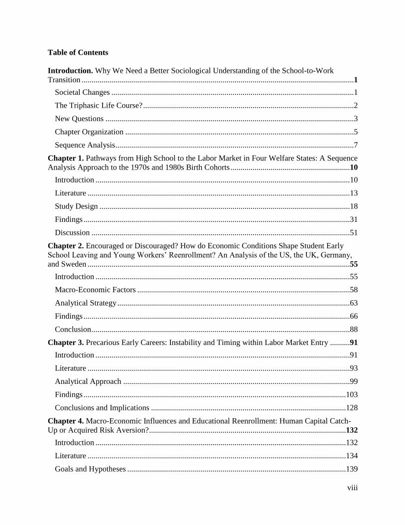
Table of Contents

Introduction. Why We Need a Better Sociological Understanding of the School-to-Work

Transition .........................................................................................................................................1

Societal Changes ..........................................................................................................................1

The Triphasic Life Course? ..........................................................................................................2

New Questions .............................................................................................................................3

Chapter Organization ...................................................................................................................5

Sequence Analysis ........................................................................................................................7

Chapter 1. Pathways from High School to the Labor Market in Four Welfare States: A Sequence

Analysis Approach to the 1970s and 1980s Birth Cohorts ............................................................10

Introduction ................................................................................................................................10

Literature ....................................................................................................................................13

Study Design ..............................................................................................................................18

Findings ......................................................................................................................................31

Discussion ..................................................................................................................................51

Chapter 2. Encouraged or Discouraged? How do Economic Conditions Shape Student Early

School Leaving and Young Workers’ Reenrollment? An Analysis of the US, the UK, Germany,

and Sweden ....................................................................................................................................55

Introduction ................................................................................................................................55

Macro-Economic Factors ...........................................................................................................58

Analytical Strategy .....................................................................................................................63

Findings ......................................................................................................................................66

Conclusion ..................................................................................................................................88

Chapter 3. Precarious Early Careers: Instability and Timing within Labor Market Entry ..........91

Introduction ................................................................................................................................91

Literature ....................................................................................................................................93

Analytical Approach ..................................................................................................................99

Findings ....................................................................................................................................103

Conclusions and Implications ..................................................................................................128

Chapter 4. Macro-Economic Influences and Educational Reenrollment: Human Capital Catch-

Up or Acquired Risk Aversion? ...................................................................................................132

Introduction ..............................................................................................................................132

Literature ..................................................................................................................................134

Goals and Hypotheses ..............................................................................................................139

ix

Data and Methods .....................................................................................................................141

Findings ....................................................................................................................................144

Discussion ................................................................................................................................162

Chapter 5. Methodological Considerations of Sequence Analysis: Algorithms, Costs, and

Clusters ........................................................................................................................................167

Sequence Analysis ....................................................................................................................167

Methodological Decisions Used in Chapter 3 ..........................................................................170

Conclusion. The Role of Social Structure and Macro-Economic Conditions on Social Inequality

at Labor Market Entry ..................................................................................................................183

Key Findings ............................................................................................................................183

Future Research ........................................................................................................................191

Appendix .....................................................................................................................................194

Appendix A (Chapter 1) ...........................................................................................................194

Appendix B (Chapter 1) ...........................................................................................................195

Appendix C (Chapter 2) ...........................................................................................................196

Bibliography ...............................................................................................................................198

x

List of Tables

Table 1. Descriptive Statistics of the Longitudinal Datasets ........................................................23

Table 2. Substitution Costs between Eight States based on Transition Rates, by country ...........29

Table 3. Time Spent in Education, Employment, and Inactivity by Decade and Country (age 16

to 25) ..............................................................................................................................................34

Table 4. Descriptive Statistics of the Labor Market Entry Clusters by Country ..........................44

Table 5. Logistic Regression on Most Precarious Labor Market Entry Cluster: United States ....46

Table 6. Logistic Regression on Most Precarious Labor Market Entry Cluster: United Kingdom

........................................................................................................................................................47

Table 7. Logistic Regression on Most Precarious Labor Market Entry Cluster: Germany ..........48

Table 8. Logistic Regression on Most Precarious Labor Market Entry Cluster: Sweden ............49

Table 9. Hazard Ratios of Leaving the Educational System for the First-Time among 16-year-

olds, United States .........................................................................................................................72


olds, United Kingdom ....................................................................................................................73


olds, Germany ................................................................................................................................74


olds, Sweden ..................................................................................................................................75


olds, by country: The Macro-Economy .........................................................................................79

Table 14. Hazard Ratios of Reentering the Educational System, by country: The Macro-

Economy ........................................................................................................................................83

Table 15. Hazard Ratios of Reentering the Educational System, by country: Occupational Status

........................................................................................................................................................86

Table 16. Hazard Ratios of Reentering the Educational System, by country: Occupational Status

and Recession Interactions .............................................................................................................87

Table 17. Overview of Identified Macro and Micro Influences on School Leaving and

Reenrollment by Country ...............................................................................................................90

Table 18. Descriptive Statistics of the Independent Variables....................................................104

Table 19. Aggregate and Monthly State Distributions ................................................................106

Table 20. Descriptive Statistics of Early Career Labor Force Trajectories ................................110

Table 21. Risk Ratios of Cluster Membership: All Pre-Entry Factors........................................115

Table 22. Risk Ratios of Cluster Membership: Macro Conditions, controlling for all pre-entry

factors ...........................................................................................................................................122

Table 23. OLS Regression Coefficients on Log-Earnings 50 months after Labor Market Entry,

Full-Time Employed ....................................................................................................................127

xi

Table 24. Means and distributions of the independent and dependent variables ........................143

Table 25. Re-entry hazard ratios of demographic factors and pre-transition factors ..................148

Table 26. Demographics-adjusted re-entry hazard ratios of individual-level labor market push

and pull factors .............................................................................................................................159

Table 27. Theoretical Substitution Costs (Version A) ...............................................................173

Table 28. Theoretical Substitution Costs (Version B) ...............................................................173

Table 29. Empirical Substitution Costs ......................................................................................173

Table 30. Pseudo R2 of Discrepancy by Algorithm, Cost Regime, and Number of Clusters ...175

Table 31. Adjusted Rand Index ..................................................................................................181

Table 32. Average Treatment Effect of Educational Reentry on Earnings at age 25 among Labor

Market Entrants during a Recession ...........................................................................................192

xii

List of Figures

Figure 1. Number of accumulated months in education (age 16 to 25) .......................................32

Figure 2. Chronograms of School to Work between Ages 16 and 25, by country ......................38

Figure 3. Chronogram of Most Precarious School to Work Trajectory between Ages 16 and 25,

by country ......................................................................................................................................42

Figure 4. Kaplan-Meier Survival Estimates in Education after age 16, by country ....................68

Figure 5. Kaplan-Meier Survival Estimates in Education after age 16 by Educational Level, by

country ...........................................................................................................................................69

Figure 6. Nelson-Aalen Cumulative Hazard Estimates of Educational Reenrollment between

ages 16 and 25, by country ...........................................................................................................81

Figure 7. Chronogram: Early Career Patterns by Cluster ..........................................................109

Figure 8. Kaplan-Meier survival estimates by subgroup ............................................................146

Figure 9. Percent-converted re-entry hazard ratios of macro labor market push and pull factors,

by educational background ..........................................................................................................153

Figure 10. Push (-) and Pull (+) education re-entry mechanisms among first-time labor market

entrants, by educational level .......................................................................................................163

Figure 11. Chronogram using Equal Substitution Costs (1) .......................................................178

Figure 12. Chronogram using Equal Substitution Costs (2) .......................................................179

Figure 13. Chronogram using Theory-based Substitution Costs (Version A) ............................180

Figure 14. Chronogram using Theory-based Substitution Costs (Version B) ...........................181

1

Introduction.

Why We Need a Better Sociological Understanding of the School-to-Work

Transition.

Societal Changes

The relationship between formal education and the labor market has changed in recent decades.

Most visible across virtually all post-industrialized countries is the increased access to higher

education and the universal expectation of high school completion. Mass higher education and

greater overall educational attainment started immediately after World War II in the United States

and around the 1960s in Western Europe. It meant that school systems rapidly adjusted to mass

rather than elite education. Programs were no longer purely academic but contained more and more

specific training to prepare students for a growing number of middle-class occupations.

Alongside the structural changes to formal education, the structure of the economy changed

dramatically which affected the character of the labor market. First, technological advancements

and accelerating international trade in the 1950s and 1960s moved the industrialized economies

from heavily reliant on the manufacturing to ones that are more oriented toward a large service-

industry economy. Second, a combination of neo-liberal policies and further globalization in 1970s

created new challenges for both firms and workers. Under pressure from international competition,

production industries called for less job protection to maintain their competitiveness. This slow

but steady deregulation of the labor market meant that employment relationships changed,

2

resulting in stagnating wages and union decline. This is called the ‘flexible turn’ (Kalleberg, 2009)

or the ‘great risk shift’ (Hacker, 2006). Its effects were most detrimental to lower-skilled and

lower-educated workers, who increasingly became exposed to job instability and job loss across

their careers (Hollister, 2011; Mishel, Bernstein, & Shierholz, 2009).

The Triphasic Life Course?

Together, the expanded educational system and the post-industrial character of the labor market

have also changed the so-called school-to-work transition. This life phase is generally understood

as the phase between formal education and stable employment. It is based on a triphasic life course

expectation: first, educational preparation, followed by an occupational career, and then

retirement. Sociological theory of labor market stratification is largely based on this triphasic life

course assumption. It allows researchers to study selection and sorting mechanisms in a quite

organized way. For instance, if two groups of similar high school graduates differ only on socio-

economic background, subsequent earnings differentials may be attributed to class inequality.

However, this simple example comparison becomes faulty when the triphasic structure of

moving from education to work is no longer the norm. In recent decades, young adults move back

and forth between the educational system and the labor market through, for instance, stopping out

of college or returning for post-graduate education at a later age. Students today tend to have longer

initial educational careers than in years past and, at the same time, return to education much more

frequently. In 2014, National Center of Education Statistics (NCES) reported that the today’s share

of adult college students (25 years or older) is about 40 percent of the student population.

3

Some social scientists have therefore stressed the outdatedness of a simple sequential route

from education to work. Instead, the modern connection between educational preparation and labor

market outcomes it is better understood if perceived as life course trajectory rather than simple

one-time transition (Bruckner & Mayer, 2005; Jacob & Weiss, 2010). The concept of a hard-cut

and one-time labor market entry has become increasingly problematic, both empirically and

theoretically.

In addition, the entire second phase of the triphasic life course, the professional career, has

become more complex as life-long occupations have disappeared from the post-industrial

economy. Several studies have shown an erosion of job ladders or internal labor markets since the

1970s, which previously provided workers with chances for future promotions and long-term

employment security within their labor market segment (DiTomaso, 2001). This has led some

scholars to argue that the lifetime employment model has been replaced by a ‘patchwork career’

in which employment relationships are only minimally connected to a profession (Mills &

Blossfeld, 2006).

New Questions

Given today’s complexity of the school-to-work transition in post-industrialized countries, the first

aim of this dissertation is to discuss the various new theoretical developments within both

educational research and labor market research. The literature reviews of the empirical chapters

attempt to show how some theoretical frameworks of education and employment overlap but have

rarely been brought together. This is partially because research on the school-to-work transition is

4

scattered across different academic fields, most importantly sociology, economics, and educational

research.

These reviews also contain a discussion of the methodologies that provide better analytical

strategies to answer new questions about social stratification within school-to-work transitions.

One relatively new methodology used in this dissertation is social sequence analysis. This

approach is particularly suited for analyzing complexity in life course data. It uses the entire time-

organized longitudinal data of individuals as the unit of analysis. More specifically, all data points

describing the positions of individuals in education or in the labor force become part of the

analysis. It therefore allows researchers to treat the trajectory from school to work holistically; to

be less focused on one transition and more focused on the complexity of maneuvering between

different positions across a longer period.

In addition to the slow but structural changes of the school-to-work phase, generations of

school leavers may enter the labor market under varying conditions. Most recently, the Great

Recession (2007 – 2009) has had an immediate and strong impact on the (youth) unemployment

rate in several countries. The impact of a rapidly rising labor surplus or macro-economic shocks

such as a recession on stratification in the labor market has not been of major concern to

sociologists; however, economists have conducted numerous studies on the effect of macro-

economic growth or downturn on the labor market. Unfortunately, their studies are not so relevant

to sociologists because they are often based on aggregate measures, thereby lacking a thorough

examination of the individual-level consequences for inequality and stratification. The analyses of

labor market outcomes in Chapters 2, 3, and 4 will therefore incorporate macro-economic

predictors of individual school-to-work trajectories: the unemployment rate and the state of the

economy (recession vs. non-recession).

5

Chapter Organization

This dissertation consists of four independent studies of different components of the school-to-

work trajectory. The first study (Chapter 1) is highly descriptive. It begins with a detailed

description of six data sources containing longitudinal data from the United States, the United

Kingdom, Germany, and Sweden. These data have been harmonized to enable thorough

international-comparative analyses in Chapters 1 and 2. It also discusses the most important

terminology as used throughout this dissertation.

The analytical question of Chapter 1 is: How do pathways between full-time education and

work vary across four ideal-typical welfare states? It should be noted that these analyses are not

meant to directly test welfare state theory. Instead, based on existing literature it raises the question

whether a welfare state regime can be recognized in the structure of the school-to-work transition.

It calls for a more comprehensive perspective on the complexity of this life phase and its

consequences for social stratification – one that supplements the current educational system

classifications and concepts of labor market segmentation. A welfare state regime perspective

provides a valuable starting point that brings educational and labor market theory together. In

doing so, the analyses of Chapter 1 also examine how school-to-work transitions have changed

over the past two decades and between these four countries. Is there evidence for convergence

between ideal-typical welfare states?

Chapter 2 builds on the conclusions of Chapter 1 that reveal similarities of the school-to-

work transition between the four countries, as well as their unique features of inequality within the

trajectory from school to work. These features include the educational attainment of different age

groups, the prevalence of educational reenrollment, and the exposure to insecure or volatile

6

(precarious) early career pathways. Using data from a wide range of birth cohorts (1970 – 1989)

this chapter answers two specific research questions concerning the connection between school

and work in different countries: (1) How do macro-economic conditions shape students’ school-

leaving probabilities? (2) Among recent school leavers, how do macro-economic conditions affect

educational reenrollment? The analyses also examine the changes over time within countries.

These studies contribute to a better understanding of how students and young members of the labor

force respond to signs of insecurity at the macro-level.

Whereas the first two chapters sacrifice some analytical precision to gain the most relevant

international-comparative research approach, both Chapters 3 and 4 are focused on just the United

States. Furthermore, the research questions apply to only one cohort – the high school population

of 1997 (National Longitudinal Study of Youth ’97) – and concentrate on the early career phase.

Chapter 3 highlights the impact of ‘precarious work’ during the labor market entry phase

of first-time school leavers. Precarious work is often defined as a position in the labor market: non-

standard work that is insecure because of the temporary basis, the poor wages, involuntary part-

time basis, or extensive night shifts (Kalleberg, 2000). This chapter reveals the longitudinal

component of precarious work: a sequence of precarious positions forming a precarious career.

These types of careers involve frequent transitions in and out of part-time work, temporary work,

and doubling-up jobs. Instability of careers has been a topic in inequality research, in which some

scholars have named this a ‘patchwork’ career (Mills & Blossfeld, 2006). Although almost all

early experience of individuals in the labor market is in some sense insecure and messy, the

analyses reveal distinct pathways between different groups of school leavers. It further suggests

that a combination of (poor) timing and early exposure to precarious work has a detrimental impact

on long-term future earnings (called ‘scarring’ by economists).

7

Chapter 4 returns to the question of educational reenrollment. It focuses primarily on two

competing theories of how school leavers respond to early career unemployment or other

problematic job-matching experiences. One theory, rooted in Human Capital Theory, predicts that

compared to a stable career pathway, increased unemployment or unemployment risk triggers a

human capital catch-up response; school leavers are more inclined to return to the educational

system to complete a degree or attain a higher level in order to improve their labor market chances

(Mroz & Savage, 2006). In contrast, if individuals perceive their future as insecure, they may

become risk averse in comparison to those in a more stable position or career prospect, which

makes them less likely to take on new risks, including educational reenrollment. This is called

‘acquired risk aversion’ (Cohn et al. 2015). The analyses in this chapter finds evidence for the

latter in response to both individual career hardships as well as macro-economic downturns. The

chapter concludes by arguing that countercyclical risk aversion further widens inequality between

lower- and higher-educated school leavers.

Sequence Analysis

All the empirical analyses conducted in this dissertation rely on longitudinal data. Each individual

record consists of a maximum of 120 monthly observations, capturing a person’s education or

labor market position: ‘enrolled’, ‘full-time employed’, ‘temporarily employed.’ All four studies

include ‘traditional’ quantitative methods of the social sciences: OLS regressions, logistic

regressions, multinomial regressions, and survival analysis (event history analysis). However, the

data also allow for social sequence analysis.

8

Sequence analysis is based on the concept of sequence alignment. Each individual’s

observation in the dataset consists of a string of unique ‘states’ (i.e. education or labor market

positions) in order of time. One can then use a cost scheme to calculate how similar two (to infinity)

sequences are; the more steps it takes to make the information strings the same, the higher the

costs, the less they look alike. Together, the sequence comparisons create a distance matrix

between all records in the dataset. Subsequently, this distance matrix can be used to cluster

comparable sequences together, thereby creating ‘ideal-types’ of trajectories.

Sequence analysis in the social sciences was criticized by sociologists in the late 1990s and

early 2000s. The most important critique was that, contrary to biological sequence analysis,

probability of being in one state or another (or transitioning from one state to another) varies across

time and is sometimes unlikely or impossible (see Wu, 2000). In short, social lives are too complex

for ‘simplistic’ cost schemes and the differences between two or more sequences cannot be

simplified into one value.

In response to these critiques, a new wave of methodological advances allows the

researcher to adjust the algorithm for different kinds of complexity (Cornwell, 2015). These

include matching algorithms that are based on the calculation of probable transitions rates based

on the common (or ‘nearby’) transitions throughout the dataset. In addition, methodologists have

gained more knowledge about the applicability of their algorithms to different types of research

questions. Simulations of different algorithms on the same data have shown some clear advantages

or disadvantages of several techniques (Halpin, 2017).

Chapter 1 and Chapter 3 further introduce social sequence analysis for the purpose of these

two studies. Chapter 5 is a methodological appendix that uses the same dataset as for the analyses

in Chapter 3. It first reviews the different (and new) social sequence analysis algorithms.

9

Subsequently, it demonstrates the options for tweaking parts of the algorithm, such as the

substitution costs or the number of clusters estimated. This section discusses the consequences of

each analytical decision for the outcomes of Chapter 3. Although methodologists still disagree on

the best way of using sequence analysis on social data, I took a pragmatic approach by comparing

each style of modeling and choosing the one that yielded realistic clusters that are most robust to

small changes in the algorithm.

10

Chapter 1.

Pathways from High School to the Labor Market in Four Welfare States.

A Sequence Analysis Approach to the 1970s and 1980s Birth Cohorts.

Introduction

Mid-twentieth century sociologists grew increasing interest in the consequences of educational

expansion and its variation across countries. Sociologists of education developed theoretical

frameworks that describe the variation in the organizational structure of modern formal schooling

and its relationship to the labor market: the school-to-work transition. Among the earliest was

Turner (1960), who presented an educational typology based on a system’s form of mobility:

‘contest’ or ‘sponsored’. Subsequent schemes clustered countries by their selection mechanism

(Hopper, 1968; Kerckhoff 2001), their impact on macro-economic development (Harbison &

Myers, 1964), and their relative role of tracking and vocational training (Shavit & Müller, 1998,

2000). Despite a multitude of school-to-work typologies, Brint (1998) states that there are only

five recurring themes in educational classification: the age of selection or transition, academic vs.

vocational schooling, the level of higher education completion, the connection between elite

schools and desired jobs, and the strength of connection between vocational curricula and jobs.

Around the same time, the comparative study of emerging welfare states theorized about

how path-dependent relationships between state, labor market, and families (or individuals) shape

socio-economic redistribution and stratification of various post-industrial countries. One of the

11

most influential principles in this field of study is the assumption that nations vary in their degree

of ‘de-commodification.’ This term refers to the extent to which social policy reduces citizens’

reliance or dependency on the erratic character of the capitalistic (labor) market that, without any

interference of the state, leads to highly uneven and extreme outcomes. Empirical research on

welfare states has focused on policy measures that directly affect the relative strength of de-

commodification, such as redistribution through taxation, social insurance, universalistic

programs, and to some extent public goods. Esping-Andersen’s (1990, 1999) typology has been

the benchmark for contemporary welfare state studies, distinguishing social-democratic states (e.g.

Sweden), corporatist states (e.g. Germany), and liberal states (e.g. United States).

The early welfare state theorist T.H. Marshall (1950) considered both social services and

education as the two institutions that facilitate the possession and distribution of ‘social rights.’

Marshall defined social rights as guaranteeing formal equality – that erase the class and status

inequalities that are formed in a capitalist system. He argued that modern societies will gradually

evolve toward a form of citizenship in which welfare benefits are equally distributed, among which

is access to the educational system.

In the decades after the publication of Marshall’s work on social rights, the concept of de-

commodification become the dominant focus rather than citizenship and its rights-based approach

to the analysis of developed capitalist countries. Moreover, influential scholars perceived

education as simply irrelevant for such cross-national research. For instance, Harold Wilensky

(1975) argued that educational policy and structures should not be included in welfare state

analysis because of its overwhelmingly meritocratic character in all developed countries. He

further argued that public expenditures on higher education are merely transfers between more and

less affluent families. Subsequently, educational policy analysis was largely absent from

12

contemporary welfare state research and theories by Esping-Andersen’s Three Worlds of Welfare

Capitalism (1990) and its successors (e.g. Walther, 2006).

In an attempt to fill a gap between theories of school-to-work transitions and welfare state

studies, this chapter presents a highly exploratory approach to examine the trajectory from the

educational system into the labor market. Scholars have used the terms ‘school-to-work trajectory,’

‘labor market entry,’ or ‘early career’ to describe the course of this life phase. These terms are

often used interchangeably. The analyses in this chapter rely on cross-national harmonized

longitudinal data that track individuals’ pathway from high school into the labor market in four

distinct welfare states: United States, United Kingdom, Germany, and Sweden. Without

investigating educational policy or structures directly, it uses a welfare state regime lens to

interpret the strong cross-country differences of these pathways.

The analyses then concentrate on signs of varying degrees of de-commodification in youth

careers across the four countries. More specifically, they reveal vulnerable (‘precarious’) labor

market positions in the first ten years after high school attendance, and assesses which social

groups are most exposed to these trajectories. The patterns of exposure to precarious work is of

great interest to the current generation of stratification researchers (Hollister, 2011). However, I

will argue that it is also relevant for the welfare state scholarship because the extent to which

societies are de-commodifying should correlate with the level of exposure to the most erratic and

precarious labor market careers.

13

Literature

Classification of education and labor markets

Traditional labor market research in economics relies on a distinction between two labor market

regimes: internal labor markets (ILMs) and occupational labor markets (OLMs). In terms of

human capital acquisition and pay-off, ILMs depend more upon on-the-job skill training compared

OLMs. Educational preparation prior to labor market entry relatively more important in OLMs.

Countries with ILMs typically offer comprehensive degrees at the secondary and tertiary level, but

they lack standardized vocational qualifications that can serve as signals to employers. In contrast,

OLMs often have standardized and specialized secondary and post-secondary programs that

prepare students for specific occupational pathways (Shavit & Müller, 1998; Marsden, 1999;

Gangl, 2003). Empirical research suggests that upward social mobility is generally greater in ILMs

than in OLMs. However, initial hiring of school leavers is easier in OLMs and therefore increases

the chance of reaching stable employment more rapidly (Brzinsky-Fay, 2007).

Scholars of the sociology of education are concerned with the initial school-to-work

transition rather than the entire work life. Among contemporary classifications of educational

systems, the most important cross-national theorization is based on the degree of standardization

and vocational training in secondary and tertiary education (Allmendinger, 1989; Brauns,

Steinmann, Kieffer & Marry, 1999; Kerckhoff, 2001; Ryan, 2001). In other words, economists and

sociologists agree on the inseparable link between formal schooling and the labor market.

Furthermore, recent empirical research based on classifications has identified quantifiable

measures of the fit or ‘linkage’ between educational programs and jobs in different countries (Bol

& Van de Werfhorst, 2013; DiPrete, Eller, Bol & Van de Werfhorst, 2017). These scholars stress

14

that countries vary in terms of the strength between specific skill acquisition in education and job

requirements (with Germany as the ideal-typical ‘strong’ linkage), and that this is positively related

to wages in many occupational fields.

Labor market entry

Numerous international-comparative studies have examined the connection between the

educational system to the labor market. The event that is most studied is the labor market entry:

the stratified outcomes of the first paid work experiences in the labor market. For instance, a great

amount of research has been conducted on the earnings pay-off of similarly educated school

leavers across different countries (Breen & Buchmann 2002; Shavit, Arum & Gamoran, 2007;

Pfeffer, 2008; Bol & Van de Werfhorst, 2011). The relative pay-off of degrees (i.e. programs)

across countries is therefore well understood in the literature.

Edited volumes by Shavit and Müller (1998) and Gangl and Müller (2003) place these early

career outcomes in a broader school-to-work transition perspective. Some studies within this

framework have focused on specific elements of the school-to-work transition, such as selection

at labor market entry (Moulin 2010) or job matching of school leavers (Van de Werfhorst, 2004).

Others have concentrated on specific educational levels and their labor market entrance: from high

school to the labor market (Rosenbaum, Kariya, Settersten & Maier, 1990; Arum & Shavit, 1995)

and from vocational school to jobs (Ianelli & Raffe, 2007).

A study by Müller (2005) provides the most comprehensive cross-country empirical

analysis of school-to-work transitions across European countries. His most important conclusion

is that more education (in length) and higher degrees are not only associated with higher class,

status, and prestige of work, but also increasingly with a lower risk of unemployment and greater

15

stability (security) of employment. The latter can also be associated with better health conditions.

Hence, bachelor’s degree graduates tend to find employment much quicker than individuals with

just secondary education, regardless of a nation’s labor market system (OLM or ILM). Educational

attainment itself is a more powerful predictor of stable labor market positions than the distinction

between general or vocational training. However, if students enter the labor market with just a

secondary school diploma, then those with specific vocational qualifications are better off.

Müller (2005) also concludes that the main labor market differentials between groups and

across countries arise in the first year after labor market entry. In this phase, he found that countries

vary consistently in terms of school leavers being to avoid unemployment. The more an

educational system provides occupational specificity, the tighter the job match, which is associated

with a lower chance of switching jobs after entering the labor market.

Early career trajectories

Beyond the initial labor market entry, the so-called early career trajectory has been an important

topic of research for both sociologists and economists. This phase has become more important as

the traditional triphasic life course – educational preparation, followed by an occupational career,

and then retirement – has disappeared in Western countries. More so than ever before, individuals

leave the educational system and yet return several months or years later, regardless of having

finished their programs. As educational careers become longer, there is also more overlap with

other life course events and adulthood phases, such as family formation. Together, the complex

overlap between education and other employment and non-employment activities is particularly

common among higher education attendees, where so-called ‘stopouts’ and post-graduate

enrollments have steadily increased.

16

As a result, the school-to-work transition is much better described as a trajectory rather

than a labor market entry – a one-time event. A commonly used methodology to understand

stratification mechanisms during this phase is to derive ideal types of early career trajectories from

entire employment histories. This line of research has led to meaningful cross-national

comparisons in Europe using social sequence analysis (Anyadike-Danes & McVicar, 2010;

Brzinsky-Fay, 2007; Scherer, 2001, 2005). Each of these studies distinguished more vulnerable or

high-precarity careers from more the stable full-time employment patterns throughout the life

course.

School leavers typically go through a job-searching phase in which they have little work

experience on their resumes. They often string together temporary jobs and internships before

finding a first (salaried) job. As argued by Brzinsky-Fay (2014), such early careers should

therefore be examined holistically – as a period within the life course – instead of as an immediate

event of switching from “in school” on one day to “employment” on the next day. In practice, only

a handful of studies concentrates on the course of school leavers in the labor market. The most

rigorous cross-national assessments examine the extent to which early careers are unstable:

moving in and out of employment or jobs (Quintini & Manfredi, 2009).

Although relevant from a descriptive point of view, sequence analysis alone cannot

examine how patterns of stratification occur regarding the (in)stability within early careers

pathways. In some studies, however, multivariate models were added to illuminate the relationship

between various demographic or socio-economic variables and post-education career trajectories.

These include school leavers in Britain in the 1980s (Anyadike-Danes & McVicar, 2005), in

Northern Ireland in the 1990s (McVicar & Anyadike-Danes, 2002), in Spain in the 2000s

17

(Corrales-Herrero & Rodríguez-Prado, 2012), where significant effects were found of parental

class (education), geography, skills (school grades), and gender on forms of early career instability.

Education and welfare state regimes

Mainstream welfare state studies have largely ignored the role of educational systems and/or the

school-to-work transition. However, some scholars have proposed mechanisms for how regime-

related structures might affect (early) careers. Estevez-Abe, Iversen, and Soskice (2001) suggest

that welfare states vary in terms of their legislative and assigned role to education. For instance, in

political rhetoric, the limited level of employment protection in liberal welfare states should

encourage individual investment in general instead of specific skills.

Others have argued that there is reason to believe that higher education could become

incorporated into Esping-Andersen’s (1990) traditional Three Worlds of Welfare Capitalism.

Without using empirical data, Willemse and De Beer (2012) reason that if one applies the idea of

de-commodification to governmental spending on (access to) public education, then welfare state

regimes types are recognized in the organization of educational systems. Brown (2001) stresses

that investment in public education is an important de-commodifying mechanism in itself.

Regimes differ in terms of distributing the costs of higher education (free systems vs. high tuition

systems), allowing educational reenrollments, and facilitating and financing of post-graduate

attainment. Furthermore, Iversen and Stephens (2008) call for the incorporation of welfare state

perspectives in examining a country’s educational system because it is the result of a

fundamentally partisan process.

A few studies have been inspired by T.H. Marshall’s original theoretical framework by

including educational ‘regulation’ in empirical research on social rights and de-commodification.

18

Studies by Eztevez-Abe, Iversen, and Soskice (2001) and Hega and Hokenmaier (2002) are

primarily concerned with comparisons of school-to-work phases across countries but they also

mention forms of regime-type influences on transitions. Taken together, these studies suggest that

corporatist regime types tend to have the highest enrollment in vocational education and more

educational differentiation because of the power of occupational groups and labor associations.

Study Design

In this chapter, the school-to-work trajectories of individuals between age 16 and age 25 are

examined. Four selected countries represent a wide range between ideal-typical regime types and

transition systems: United States (liberal), United Kingdom (liberal), Germany (corporatist), and

Sweden (social-democratic). The first series of analyses rely on exploratory methods to answer

questions regarding the structure of this life course phase: How do these four countries differ in

terms of their pathways between full-time secondary education and the labor market? And,

are precarious early careers more prevalent in the low de-commodification countries?

No previous study has been conducted on internationally-comparative longitudinal records

of individuals’ pathway from secondary education to their mid-twenties. Regime theory provides

some initial expectations regarding cross-national differences of early career stratification: liberal

welfare states should tend to have less regulation and protection of labor than social-democratic

and corporatist regimes. The influence of market forces in liberal regimes is generally higher

because social security policy and unions are less protective of workers and their families. As ‘de-

commodification’ is lowest in liberal states, a higher prevalence of more insecure work positions

19

is expected for the school-to-work trajectories of United States and the United Kingdom, in

comparison to Germany and Sweden. These include doubling-up part-time jobs, self-employment,

temporary jobs, and a pattern of going in and out of non-employment.

Social-democratic regimes, such as Sweden, have more universalistic and generous

policies to protect workers from losing their employment or having immediate financial difficulties

in case of job-loss. Young individuals in the labor market are often most vulnerable to such

positions, but when the same age group is compared across countries, there should be observable

differences between countries’ typical trajectories from school to work. Specifically, careers in

liberal regimes should look most insecure, followed by those in corporatist regimes, and the least

volatile in social-democratic regimes.

Another theoretical framework helps to turn ‘vulnerable positions in the labor market’ or

‘market dependency’ into more explicit and assessable concepts. Inequality scholars use the term

‘precarious work’ to describe work that is characterized by a profound uncertainty about income

and an enduring risk of unemployment. Moreover, precarious jobs have relatively lower wages

and typically lack all kinds of benefits, such as medical coverage and pensions, which adds another

element to workers’ vulnerable positions (Kalleberg, 2009; 2011). Using this definition, low de-

commodification countries should have greater amounts of precarious work. One key feature of

precarious work is that it refers to both a state – a vulnerable employment position – as well as an

expected unstable pattern in labor market position. Hence, a labor market in which careers are

‘precarious’ not only consists of an insecure position or job at one moment in time, but also of a

high level of job switching, moving in and out of part-time and unemployment over time. The

longitudinal character of individual-level harmonized education and labor market histories enables

sequence analysis to reveal these precarious youth careers.

20

The analyses will then turn to the question: How have the trajectories between school

and work changed over time? Have they become more or less precarious? Again, in addition

to the concept of precarious early careers, welfare state theory provides a relevant starting point to

study the possible changing character of the school-to-work pathway over the last decades. Some

scholars have suggested that despite the path-dependency nature of welfare states, there is

convergence between countries with different regime types. Although the claim of welfare state

convergence is contested by some scholars, there is evidence for more converging in aggregate

expenditures on social security between regime types. Studies by Achterberg and Yerkes (2009)

and Schmitt and Stark (2011) suggest that social-democratic countries have become more

‘liberalized’ or ‘neo-liberal’ while, at the same time, liberal welfare states have slowly become

more universal. This group of scholars argue that convergence is caused by economic globalization

to which welfare state structures respond in opposite ways. As a result, the school-to-work phase

of the youngest cohorts of labor market entrants should consist of more instability compared to

older cohorts in liberal welfare states (United States and United Kingdom), and vice-versa in

social-democratic welfare states (Sweden) or corporatist welfare states (Germany).

Finally, the analyses will reveal: Which demographic backgrounds and social groups

are most likely to be exposed to precarious work? Although job precarity has increased over

time for virtually every type of worker, some groups are much more vulnerable for such

employment than others (Kalleberg, 2012). This is particularly the case for lower-educated and

lower-skilled workers, who are more likely to have fixed-term contracts and to experience

unemployment, and more than previous cohorts (DiPrete, 2005). In comparison to whites, all

ethno-racial minority groups are more likely to be exposed to unemployment and displacement

from work (Kalleberg, 2009). Kogan (2007) also found that immigrant groups have vastly different

21

career trajectories than their non-immigrant counterparts. Although most men of immigrant

descent are employed in lower-skilled segments of the labor market, their precarious careers

cannot be fully explained by their educational background or human capital. There is however no

existing evidence as to whether these associations vary across countries.

Data

The data combine several large longitudinal datasets that capture the month-to-month positions in

education and in the labor market; from the compulsory school age thru the early work life of

individuals until age 25. The selected datasets include several different birth cohorts (1960s thru

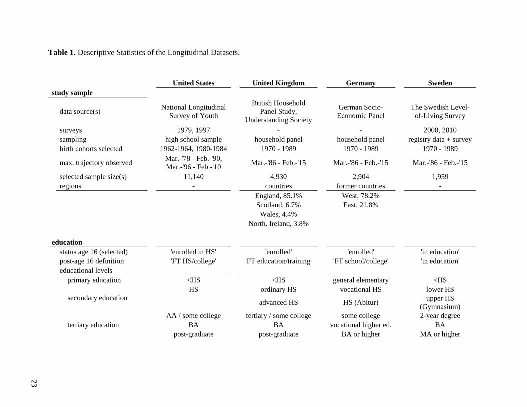
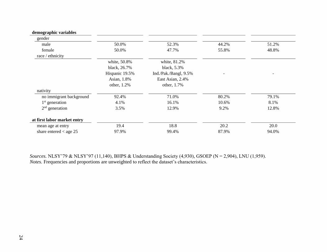
1980s) which allows analyses of changes in the school-to-work trajectories over time. Table 1

summarizes the details of the selected datasets for each country, as well as some unique descriptive

features of their educational variables and demographic variables.

The data from the United States consist of two samples of the National Longitudinal Survey

of Youth (NLSY), both 1979 and 1997. Both studies follow a representative sample of high school

students between the ages of 12 and 16 all the way into their adult lives (Bureau of Labor Statistics

2014, 2015). Individuals were interviewed on an annual basis for the first 15 years. These

respondents are still being interviewed on a biannual basis until today.

The data from the United Kingdom are drawn from two data sources. One part comes from

the British Household Panel Study (BHPS), which ran between 1991 and 2007 (Taylor, 2010).

The other part is drawn from its successor, Understanding Society (US), which a similar household

panel that was first interviewed in 2008 (University of Essex, 2017). The BHPS is a household-

based sample that initially covered residents of England and Wales. Households from Scotland

and Northern Ireland were added in the late 1990s.

22

The German data are drawn from the similarly organized German Socio-Economic Panel

(GSOEP). These respondents were first sampled in order to represent West-German households in

1984. Respondents from former East-Germany were added to the sample after reunification

(Wagner, Frick & Schupp, 2007). The children of original members of the panel were

automatically included in the sample upon reaching adulthood.

The data from Sweden consist of two randomly selected individual-level samples (2000,

2010) on which elaborate interviews were conducted about work, education, health, and family.

These studies are called the Level of Living Surveys or Levnadsnivåundersökningarna (LNU).

Subsequently, the individual cases were matched with national registry data, which documents

individuals’ entire employment histories (Stockholm Universitet, 2010).

23

Table 1. Descriptive Statistics of the Longitudinal Datasets.

United States United Kingdom Germany Sweden

study sample

data source(s) National Longitudinal

Survey of Youth

British Household

Panel Study,

Understanding Society

German Socio-

Economic Panel The Swedish Level-

of-Living Survey

surveys 1979, 1997 - - 2000, 2010 sampling high school sample household panel household panel registry data + survey birth cohorts selected 1962-1964, 1980-1984 1970 - 1989 1970 - 1989 1970 - 1989

max. trajectory observed Mar.-'78 - Feb.-'90,

Mar.-'96 - Feb.-'10 Mar.-'86 - Feb.-'15 Mar.-'86 - Feb.-'15 Mar.-'86 - Feb.-'15

selected sample size(s) 11,140 4,930 2,904 1,959 regions - countries former countries - England, 85.1% West, 78.2%

Scotland, 6.7% East, 21.8%

Wales, 4.4%

North. Ireland, 3.8%

education status age 16 (selected) 'enrolled in HS' 'enrolled' 'enrolled' 'in education' post-age 16 definition 'FT HS/college' 'FT education/training' 'FT school/college' 'in education' educational levels primary education <HS <HS general elementary <HS

secondary education

HS ordinary HS vocational HS lower HS

advanced HS HS (Abitur) upper HS

(Gymnasium)

tertiary education

AA / some college tertiary / some college some college 2-year degree BA BA vocational higher ed. BA post-graduate post-graduate BA or higher MA or higher

24

demographic variables gender male 50.0% 52.3% 44.2% 51.2% female 50.0% 47.7% 55.8% 48.8% race / ethnicity white, 50.8% white, 81.2%

black, 26.7% black, 5.3%

Hispanic 19.5% Ind./Pak./Bangl, 9.5% - - Asian, 1.8% East Asian, 2.4%

other, 1.2% other, 1.7%

nativity no immigrant background 92.4% 71.0% 80.2% 79.1% 1st generation 4.1% 16.1% 10.6% 8.1% 2nd generation 3.5% 12.9% 9.2% 12.8%

at first labor market entry mean age at entry 19.4 18.8 20.2 20.0 share entered < age 25 97.9% 99.4% 87.9% 94.0%

Sources. NLSY’79 & NLSY’97 (11,140), BHPS & Understanding Society (4,930), GSOEP (N = 2,904), LNU (1,959).

Notes. Frequencies and proportions are unweighted to reflect the dataset’s characteristics.

25

Only individuals born between 1970 and 1989 were selected for the final study sample.

This is the largest possible length of birth cohorts across countries and covers exactly two decades.

However, the data from the United States create a slightly different distribution of birth cohorts.

The NLSY data consist of two studies with birth cohorts 1962-1964 (NLSY’79) and 1980-1984

(NLSY’97), which allows a simpler comparison between a 1960s and a 1980s cohort. The fifth

row of the top panel of Table 1 indicates the corresponding school-to-work trajectory years

observed.

With exception of the NLSY data, each longitudinal dataset is supplemented with new

cases on several occasions to keep the dataset both large and representative. Moreover, children in

the already-sampled households typically become independent respondents once they become an

adult. Each country-specific dataset is known for its relatively low attrition rate. Nonetheless, the

study samples used in this paper are substantially smaller than the original household panels of the

United Kingdom and Germany. This is the result of selecting only respondents who have

employment histories that are reliable (not more than 20 gaps), long enough (at least 90 monthly

observations between age 16 and 25) and fall within the selected birth cohorts: 1970 thru 1989.

Respondents are selected for the study sample conditional on the availability of their

education (or work) status at age 16. The t-1 observation of each selected respondent is ‘enrolled

in full-time education’ in March of the year in which he or she turned 16 – a mid-semester month

to avoid the traditional Summer and Winter breaks. Any first observed non-full-time education

position is considered a labor market entry if the non-full-time enrollment spell was longer than

seven months (more than one semester). Otherwise, it is assumed that an individual was not

enrolled for just a few months. This conservative definition does therefore not capture the smallest

‘stopouts’ or longer breaks. Any next observation of education – after the initial transition from

26

full-time education to the labor market – is only coded as ‘education’ if one’s status is another full-

time enrollment in high school, college, or training (slightly different across countries).

Beyond the initial school-to-work transition, the full trajectory between day-time

education and the labor market experience is mapped in a sequential order for each respondent.

These so-called ‘states’ are measured (coded) as an individual’s main activity for each month

between age 16 and 25 – a total of 120 monthly observations. For the purpose of studying

stratification and market-dependency, the categorization is not only determined by the availability

of data in each country’s dataset, but also by a creating a variation of stronger and weaker labor

market positions. Despite the availability of much more complex state categorizations, the

sequence data are harmonized to reflect eight possible positions: full-time education, full-time

employment, any part-time employment (a category that also includes any form of temporary

employment), self-employed, any social service (including military), unemployed, inactive, and

long-term sick.

Some analyses are conducted by highest educational attainment: secondary only, higher

education only, and bachelor’s degree attaining (not mutually exclusive). Models predicting labor

market outcomes control for highest educational level completed measured at age 25. The country-

specific categorical variables presented in second panel of Table 1. These variables are constructed

to allow for the best possible comparison of the bachelor’s degree level (or equivalent) and higher,

as well as the relevant lower tertiary levels and the high school diplomas.

The third panel of Table 1 presents the most important individual-level demographic

variables. The race (+ ethnicity) variable is country-specific and are only available for the US and

UK datasets. Both countries oversampled their respective racial- and ethnic minorities. The

categories for the 1st and 2nd generations in the immigrant background variable consist of different

27

ethnic groups. The immigrant population in Germany consists largely of Turks, whereas the

Swedish 1st and 2nd generations are predominantly Middle Eastern (Iraq, Iran, and Syria) and

Finnish. The GSOEP (Germany) oversampled immigrants of the 1st- and 2nd-generations.

The frequencies reported in Table 1 figures are unweighted, but sampling weights applied

to all multivariate prediction models to represent the populations. The proportion of US

respondents who are immigrants and children of immigrants will remain a bit lower than the

national average. This is a result of the sampling representing high school students instead of

households.

Methods

After harmonizing the individual records across a ten-year period some gaps (states) needed to be

imputed. Since the selection of cases for this study is conditional on knowing one’s status in the

Spring of the year in which a respondent turned 16 (and this being ‘in full-time education’), only

two types of missing states occurred in the data: internal missing (‘gaps’) and right-censoring.

Missing states in sequence data may also be coded as a separate category, but simulations by

Halpin (2012) proved the superiority of MICT: multiple imputation for categorical time-series.

This Stata application was used to impute up to 20 internal monotone and non-monotone gaps of

an individual sequence. Any sequence that contains more missingness was excluded from the

analysis.

Subsequently, the Optimal Matching algorithm available in the SADI-package for Stata

(Halpin, 2017) was used to calculate the distance between each individual’s pathway in school and

the labor market between the ages of 16 and 25. This distance measure is based on the idea that

the fewer steps that are necessary to make a set of two sequences equal, the more similar those

28

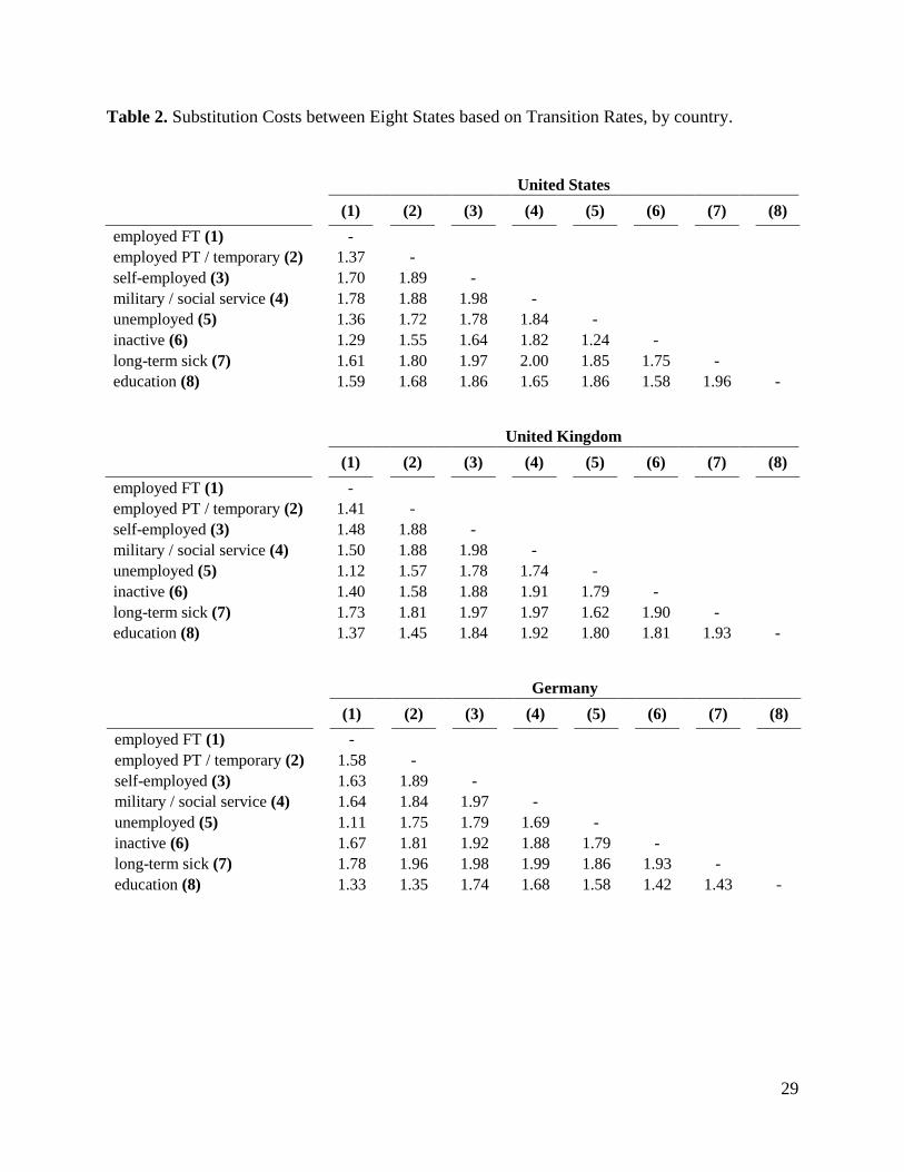
sequences are. These steps can be calculated using so-called indel costs (for extending or

shortening spells) substitution costs (for replacing one state with another). The indel costs were set

at 1 and the substitution costs were generated empirically by calculating the transition probabilities

of labor market states. Table 2 documents the cost distributions between the eight states, for each

country separately. These cost distributions are derived from the transition matrix; the relative

probabilities of moving from one state to another across the entire observation length.1

Sequence analysis provides a distance measure between each respondent’s pathway from

school to work and each other pathway. The Ward algorithm was then used to estimate clusters of

similar trajectories. Although there is no particular reason for why there could not be an infinite

number of clusters, for the purpose of manageability and sociologically interpretability, between

five and seven clusters were attempted (Brzinsky-Fay, 2007). Several different approaches were

attempted in terms of cost-scheme, number of clusters, and matching algorithm. This process, as

well as a broader discussion of debates in sequence analysis research, is described in detail in the

methodological appendix chapter (Chapter 5) of this dissertation. The main advantage of sequence

analysis is that it examines individual records as holistic entities. In contrast to a prediction of an

outcome at time two based on a set of variables measured at time one, there is limited loss of

information in records that exist of many – hundreds or even thousands – of subsequent time

observations. It is therefore well suited for initial exploratory sociological questions about

pathways and trajectories within in the life course.

1 However, high costs between two states reflect a low (unlikely) transition rate and vice versa.

29

Table 2. Substitution Costs between Eight States based on Transition Rates, by country.

United States

(1) (2) (3) (4) (5) (6) (7) (8)

employed FT (1) -

employed PT / temporary (2) 1.37 -

self-employed (3) 1.70 1.89 -

military / social service (4) 1.78 1.88 1.98 -

unemployed (5) 1.36 1.72 1.78 1.84 -

inactive (6) 1.29 1.55 1.64 1.82 1.24 -

long-term sick (7) 1.61 1.80 1.97 2.00 1.85 1.75 -

education (8) 1.59 1.68 1.86 1.65 1.86 1.58 1.96 -

United Kingdom

(1) (2) (3) (4) (5) (6) (7) (8)

employed FT (1) -




unemployed (5) 1.12 1.57 1.78 1.74 -

inactive (6) 1.40 1.58 1.88 1.91 1.79 -

long-term sick (7) 1.73 1.81 1.97 1.97 1.62 1.90 -

education (8) 1.37 1.45 1.84 1.92 1.80 1.81 1.93 -

Germany

(1) (2) (3) (4) (5) (6) (7) (8)

employed FT (1) -




unemployed (5) 1.11 1.75 1.79 1.69 -

inactive (6) 1.67 1.81 1.92 1.88 1.79 -

long-term sick (7) 1.78 1.96 1.98 1.99 1.86 1.93 -

education (8) 1.33 1.35 1.74 1.68 1.58 1.42 1.43 -

30

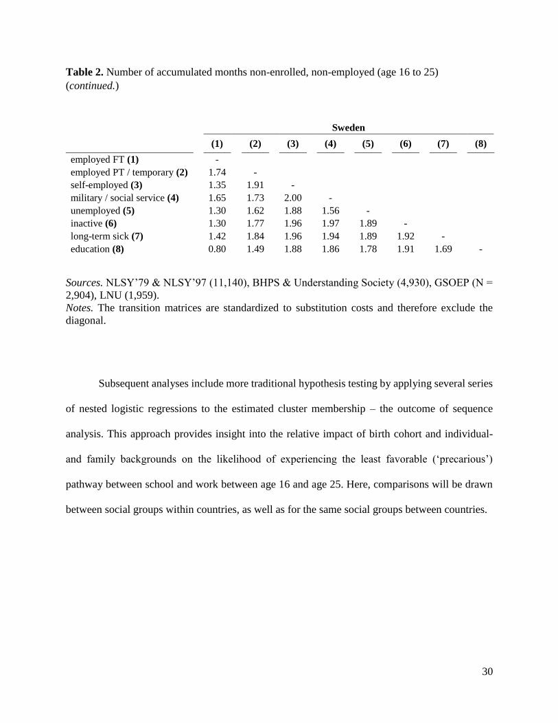
Table 2. Number of accumulated months non-enrolled, non-employed (age 16 to 25)

(continued.)

Sweden

(1) (2) (3) (4) (5) (6) (7) (8)

employed FT (1) -




unemployed (5) 1.30 1.62 1.88 1.56 -

inactive (6) 1.30 1.77 1.96 1.97 1.89 -

long-term sick (7) 1.42 1.84 1.96 1.94 1.89 1.92 -

education (8) 0.80 1.49 1.88 1.86 1.78 1.91 1.69 -

Sources. NLSY’79 & NLSY’97 (11,140), BHPS & Understanding Society (4,930), GSOEP (N =

2,904), LNU (1,959).

Notes. The transition matrices are standardized to substitution costs and therefore exclude the

diagonal.

Subsequent analyses include more traditional hypothesis testing by applying several series

of nested logistic regressions to the estimated cluster membership – the outcome of sequence

analysis. This approach provides insight into the relative impact of birth cohort and individual-

and family backgrounds on the likelihood of experiencing the least favorable (‘precarious’)

pathway between school and work between age 16 and age 25. Here, comparisons will be drawn

between social groups within countries, as well as for the same social groups between countries.

31

Findings

Educational careers

Educational systems have a strong impact on the average time spent in education and the labor

market during the early career phase. Some of the school- and work-contrasts across countries are

structural; a direct function of how educational programs and policies are designed. Other features

of the school-to-work trajectory change over time. For instance, educational expansion has

influenced all four countries’ pathways, but not in the same way. This section will briefly discuss

both the structural characteristics of the educational enrollment until age 25, as well as the dramatic

changes over time.

Figure 1 plots the average number of months spent in full-time education between ages 16

and 25, by birth cohort and country. The total number of months in this ten-year period is 120 (x-

axis). The grey solid line represents the US data that only captures the mid-1960s and mid-1980s

birth cohorts of the NLSY’s. It nonetheless shows a clear increase of educational enrollment from

just under 50 months to just under 60 months (out of 120 months). Although no panel data of the

1960s birth cohorts in the other three countries are plotted here, it is well-documented that the

United States’ educational system expanded first and was presumably still ahead in terms of

accumulated enrollment months among its respective 1960s birth cohorts.

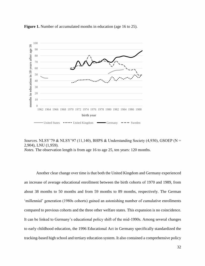
32

Figure 1. Number of accumulated months in education (age 16 to 25).


2,904), LNU (1,959).

Notes. The observation length is from age 16 to age 25, ten years: 120 months.

Another clear change over time is that both the United Kingdom and Germany experienced

an increase of average educational enrollment between the birth cohorts of 1970 and 1989, from

about 38 months to 50 months and from 59 months to 89 months, respectively. The German

‘millennial’ generation (1980s cohorts) gained an astonishing number of cumulative enrollments

compared to previous cohorts and the three other welfare states. This expansion is no coincidence.

It can be linked to Germany’s educational policy shift of the mid-1990s. Among several changes

to early childhood education, the 1996 Educational Act in Germany specifically standardized the

tracking-based high school and tertiary education system. It also contained a comprehensive policy

0

10

20

30

40

50

60

70

80

90

100

1962 1964 1966 1968 1970 1972 1974 1976 1978 1980 1982 1984 1986 1988

mo

nth

s in

ed

uca

tio

n i

n 1

0 y

ears

aft

er a

ge

16

birth year


33

effort to improve ‘lifelong learning’ through, for instance, the formalization of vertical transitions

(Beutner & Pecheul, 2017). These allow students to move from one level of education to another

without interruptions.

Sweden displayed the highest average educational enrollment until age 25 in 1970,

followed the expected indication of educational expansion with more than half of the time between

age 16 and 25 spent in full-time education. However, Swedish respondents born in the 1980s show

slightly lower attainment averages in this graph. This dip on the far-right of the graph should not

be overstated because there are far fewer 1985-1989 respondents in this sample compared to earlier

cohorts and compared to other countries. Nonetheless, the Swedish educational system has

undergone significant changes toward a more decentralized (and pluralist) organization since the

early-1990s (Hartman, 2007). These policy shifts may partially explain the stagnation (or decline)

of educational participation, but there is no direct evidence to support this.

Table 3 splits the percent of monthly states in education, employment, and NEET (not in

education, employment, or training) by decade of birth year. The share spent in education reflects

the results from Figure 1. Time spent in employment positions, either full-time or part-time, is

relatively stable over time, yet structurally much higher in the United Kingdom: around 46 percent

of the observed ten-year careers, compared to roughly 25 to 30 percent in other countries.

Furthermore, the increased level of educational attainment in Germany between the 1970s and

1980s cohorts coincides with a sharp drop in time spent in employment. Youths under 25 in the

United States spent about 8 to 10 percent in NEET since high school age, which is substantially

more than in the other three countries.

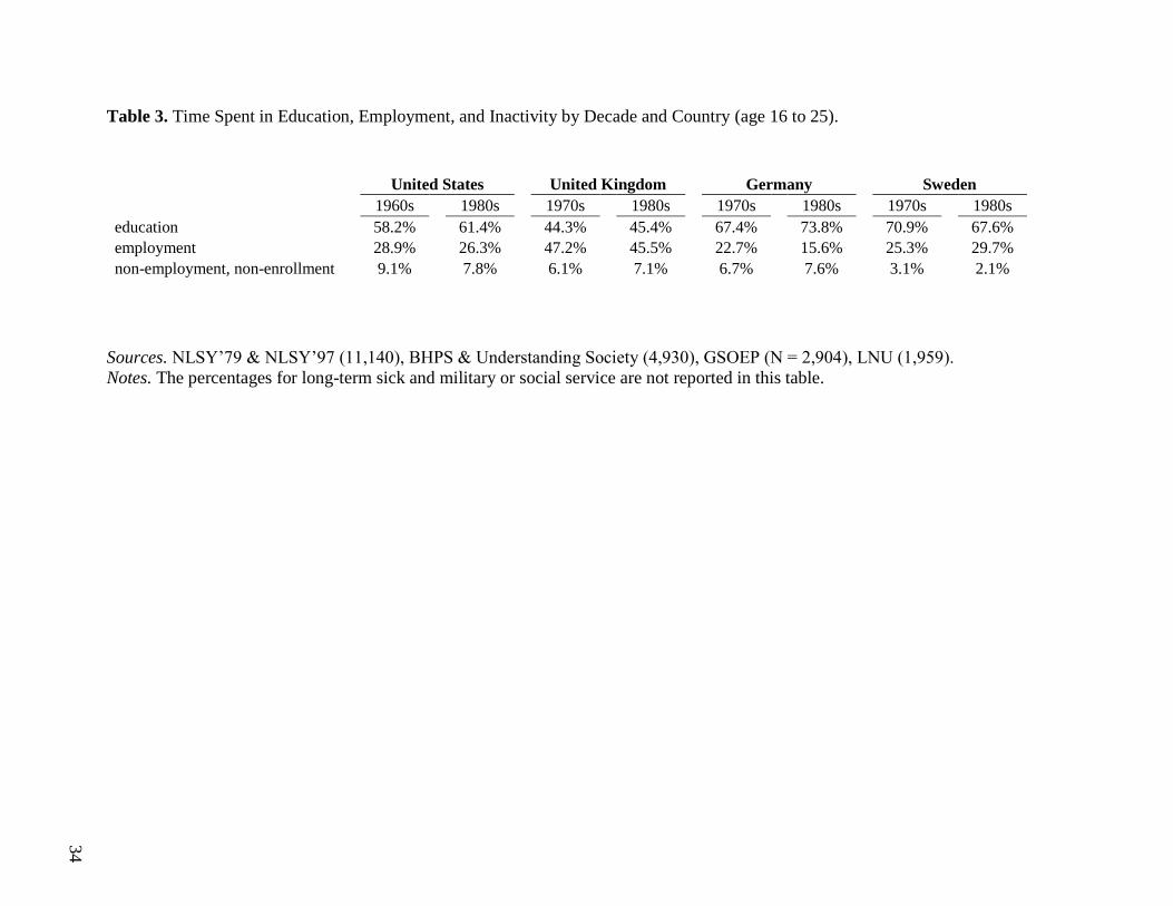
34

Table 3. Time Spent in Education, Employment, and Inactivity by Decade and Country (age 16 to 25).

United States United Kingdom Germany Sweden 1960s 1980s 1970s 1980s 1970s 1980s 1970s 1980s

education 58.2% 61.4% 44.3% 45.4% 67.4% 73.8% 70.9% 67.6%

employment 28.9% 26.3% 47.2% 45.5% 22.7% 15.6% 25.3% 29.7%

non-employment, non-enrollment 9.1% 7.8% 6.1% 7.1% 6.7% 7.6% 3.1% 2.1%


Notes. The percentages for long-term sick and military or social service are not reported in this table.

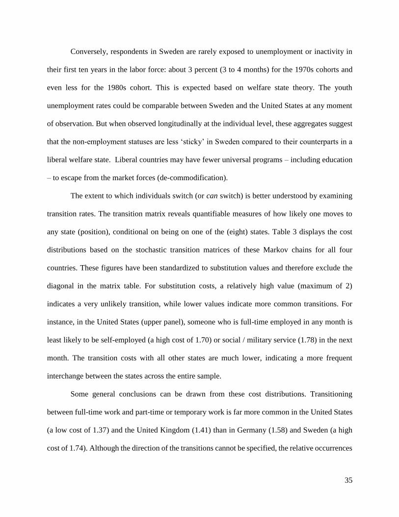
35

Conversely, respondents in Sweden are rarely exposed to unemployment or inactivity in

their first ten years in the labor force: about 3 percent (3 to 4 months) for the 1970s cohorts and

even less for the 1980s cohort. This is expected based on welfare state theory. The youth

unemployment rates could be comparable between Sweden and the United States at any moment

of observation. But when observed longitudinally at the individual level, these aggregates suggest

that the non-employment statuses are less ‘sticky’ in Sweden compared to their counterparts in a

liberal welfare state. Liberal countries may have fewer universal programs – including education

– to escape from the market forces (de-commodification).

The extent to which individuals switch (or can switch) is better understood by examining

transition rates. The transition matrix reveals quantifiable measures of how likely one moves to

any state (position), conditional on being on one of the (eight) states. Table 3 displays the cost

distributions based on the stochastic transition matrices of these Markov chains for all four

countries. These figures have been standardized to substitution values and therefore exclude the

diagonal in the matrix table. For substitution costs, a relatively high value (maximum of 2)

indicates a very unlikely transition, while lower values indicate more common transitions. For

instance, in the United States (upper panel), someone who is full-time employed in any month is

least likely to be self-employed (a high cost of 1.70) or social / military service (1.78) in the next

month. The transition costs with all other states are much lower, indicating a more frequent

interchange between the states across the entire sample.

Some general conclusions can be drawn from these cost distributions. Transitioning

between full-time work and part-time or temporary work is far more common in the United States

(a low cost of 1.37) and the United Kingdom (1.41) than in Germany (1.58) and Sweden (a high

cost of 1.74). Although the direction of the transitions cannot be specified, the relative occurrences

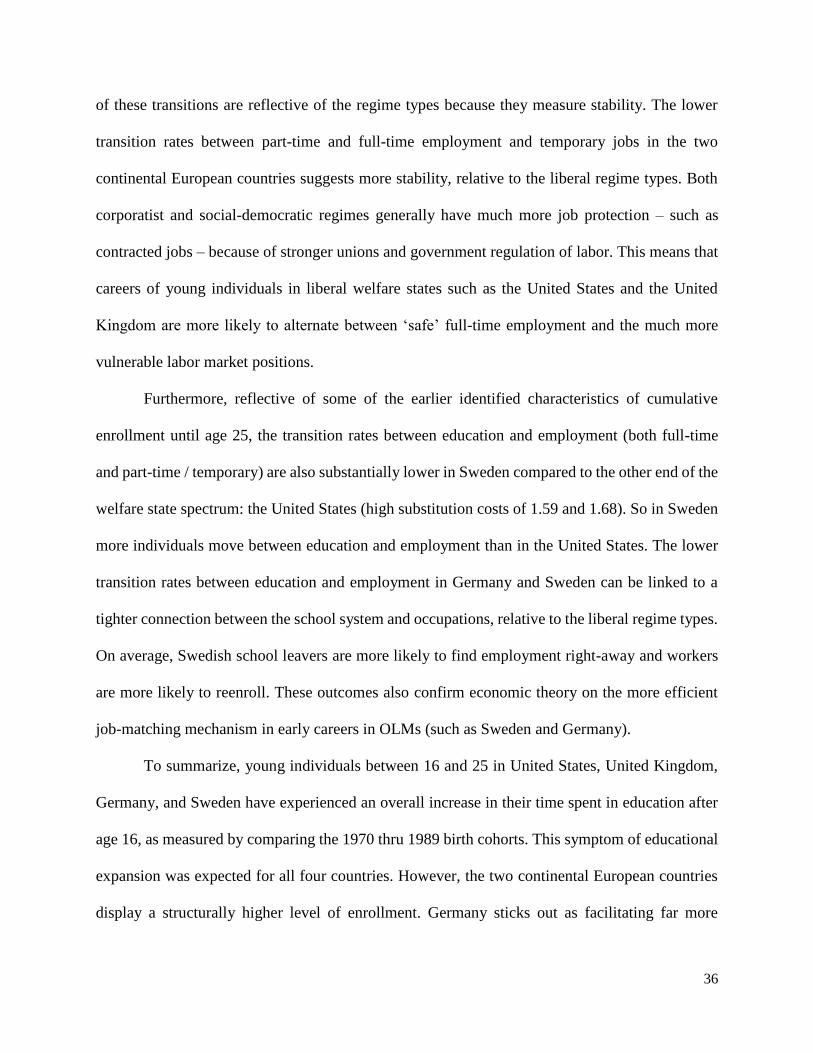
36

of these transitions are reflective of the regime types because they measure stability. The lower

transition rates between part-time and full-time employment and temporary jobs in the two

continental European countries suggests more stability, relative to the liberal regime types. Both

corporatist and social-democratic regimes generally have much more job protection – such as

contracted jobs – because of stronger unions and government regulation of labor. This means that

careers of young individuals in liberal welfare states such as the United States and the United

Kingdom are more likely to alternate between ‘safe’ full-time employment and the much more

vulnerable labor market positions.

Furthermore, reflective of some of the earlier identified characteristics of cumulative

enrollment until age 25, the transition rates between education and employment (both full-time

and part-time / temporary) are also substantially lower in Sweden compared to the other end of the

welfare state spectrum: the United States (high substitution costs of 1.59 and 1.68). So in Sweden

more individuals move between education and employment than in the United States. The lower

transition rates between education and employment in Germany and Sweden can be linked to a

tighter connection between the school system and occupations, relative to the liberal regime types.

On average, Swedish school leavers are more likely to find employment right-away and workers

are more likely to reenroll. These outcomes also confirm economic theory on the more efficient

job-matching mechanism in early careers in OLMs (such as Sweden and Germany).

To summarize, young individuals between 16 and 25 in United States, United Kingdom,

Germany, and Sweden have experienced an overall increase in their time spent in education after

age 16, as measured by comparing the 1970 thru 1989 birth cohorts. This symptom of educational

expansion was expected for all four countries. However, the two continental European countries

display a structurally higher level of enrollment. Germany sticks out as facilitating far more

37

educational enrollment for its youngest generation of students. Sweden can be identified as a

social-democratic regime type where youths are less exposed to NEET and maneuvering in and

out of part-time or temporary work. Instead, education in Sweden seems linked tighter to full-time

employment, which is associated with stability over time.

Chronograms reflecting the school-to-work trajectory

Both cumulative time spent in states and transition probabilities are helpful tools to understand the

general character of education, work, and forms of inactivity. These measures are however crude

compared to the complexity within individual careers. The descriptive statistics from sequence

analysis reveals the entire school-to-work pathway; holistically – as a trajectory rather than

measuring group aggregates or a series of observations (t-1 vs. t-2).

One strong visual descriptive of longitudinal data is a chronogram. It graphs the time-

dependent state distribution, thereby including all respondents (rows) and time observations (120

months in this case). Figure 2 present the chronograms of the school-to-work phase between age

16 and 25 for each country. The chronograms display the distribution among the eight selected

states by time period – each vertical ‘slice’ reflecting a monthly observation. Reading from left to

right, one finds fewer education positions (beige) and an increasing number of full-time

employment positions (blue) over time, as expected.

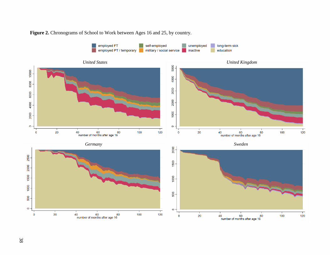
38

Figure 2. Chronograms of School to Work between Ages 16 and 25, by country.

United States United Kingdom

Germany Sweden

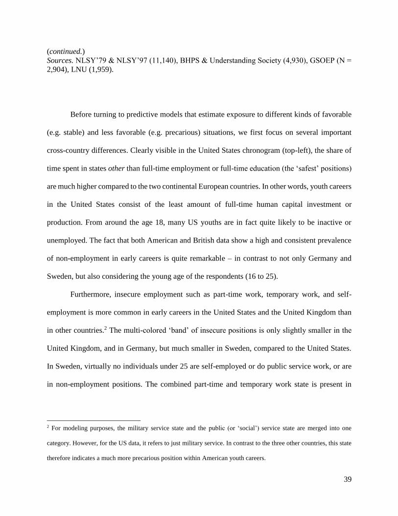
39

(continued.)


2,904), LNU (1,959).

Before turning to predictive models that estimate exposure to different kinds of favorable

(e.g. stable) and less favorable (e.g. precarious) situations, we first focus on several important

cross-country differences. Clearly visible in the United States chronogram (top-left), the share of

time spent in states other than full-time employment or full-time education (the ‘safest’ positions)

are much higher compared to the two continental European countries. In other words, youth careers

in the United States consist of the least amount of full-time human capital investment or

production. From around the age 18, many US youths are in fact quite likely to be inactive or

unemployed. The fact that both American and British data show a high and consistent prevalence

of non-employment in early careers is quite remarkable – in contrast to not only Germany and

Sweden, but also considering the young age of the respondents (16 to 25).

Furthermore, insecure employment such as part-time work, temporary work, and self-

employment is more common in early careers in the United States and the United Kingdom than

in other countries.2 The multi-colored ‘band’ of insecure positions is only slightly smaller in the

United Kingdom, and in Germany, but much smaller in Sweden, compared to the United States.

In Sweden, virtually no individuals under 25 are self-employed or do public service work, or are

in non-employment positions. The combined part-time and temporary work state is present in

2 For modeling purposes, the military service state and the public (or ‘social’) service state are merged into one

category. However, for the US data, it refers to just military service. In contrast to the three other countries, this state

therefore indicates a much more precarious position within American youth careers.

40

Swedish early careers, and is comparable in size to the other countries. However, its share grows

much later on in the ten-year course after age 16 – around month 45 (age 20).

Together, these visual representations of typical trajectories in education and the labor

market suggest strong inter-country differences, with the United States and Sweden as the two

extremes on a four-country ‘spectrum.’ Young individuals who enter the labor market in the United

States are more likely to do so when they are younger, compared Swedish youths at the other end

of the spectrum. Moreover, Americans (and Brits) are exposed to much more non-employment as

well as lengthy precarious spells before age 25. These experiences do exist in Germany and

Sweden, but to a much less frequently and tend to occur when they are a bit older (20 years of

age). The next section will further unpack the insecure or ‘precarious’ trajectories.

Precarity during labor market entry

To examine the extent to which young individuals are exposed to precarity in the labor market,

sequence analysis in combination with OM cluster analysis was applied to each country’s dataset.

The researcher decides on the number of clusters to be estimated. Here, three or four clusters per

country were attempted and then evaluated using their pseudo R-squares (see Chapter 5) using and

entropy levels of the clusters (bottom row of Table 4). Which cluster is labeled as (most)

‘precarious’ is however based on a qualitative assessment of the share of undesirable positions

(e.g. unemployment, inactivity, and long-term illness), the pattern of moving in and out of part-

time or temporary work, and the stability of careers. The latter is measured quantitatively by

calculating the number average number of spells (or transitions) across the observed ten-year

period. The non-precarious clusters consist of trajectories with either long-term enrollment in

higher education (a ‘slow labor market entry’) or a stable pattern of full-time work (a ‘fast labor

41

market entry’). Appendix A plots the chronograms of these two contrasting pathways for just the

United States (because the three other countries had very similar outcomes).

The analysis will concentrate on the vulnerable trajectories. Figure 3 plots the chronograms

of each country’s most ‘precarious’ school-to-work pathway from age 16 to age 25. Although each

country has an identifiable vulnerable cluster, the chronograms of the United States and the United

Kingdom display much stronger exposure to unstable work and volatile career experiences. That

is, the share of inactivity, unemployment, and part-time or temporary work remains large

throughout the observed ten-year period (including military service in the US data). Moreover, a

large proportion of school leavers are clustered in the high-precarious ideal type: 42.8% (United

States) and 51.7% (United Kingdom).

In contrast, Germany’s most precarious trajectory is small (14.8% of the sample) and is

primarily based on exposure to temporary work and part-time work for a long period of time, even

though some of this trajectory still includes full-time education. The clustering algorithms only

recognized a small cluster (19.5%) of vulnerable pathways from school to work in the Swedish

data. Even though the size of the precarious cluster in Sweden is small, it consists mostly of

unemployment and inactivity (but not part-time work and temporary work). If we were to speculate

on how these country-differences can be explained, the relatively stronger job protection policies

in a social-democratic regime like Sweden may make temporary work less prevalent, even in youth

careers.

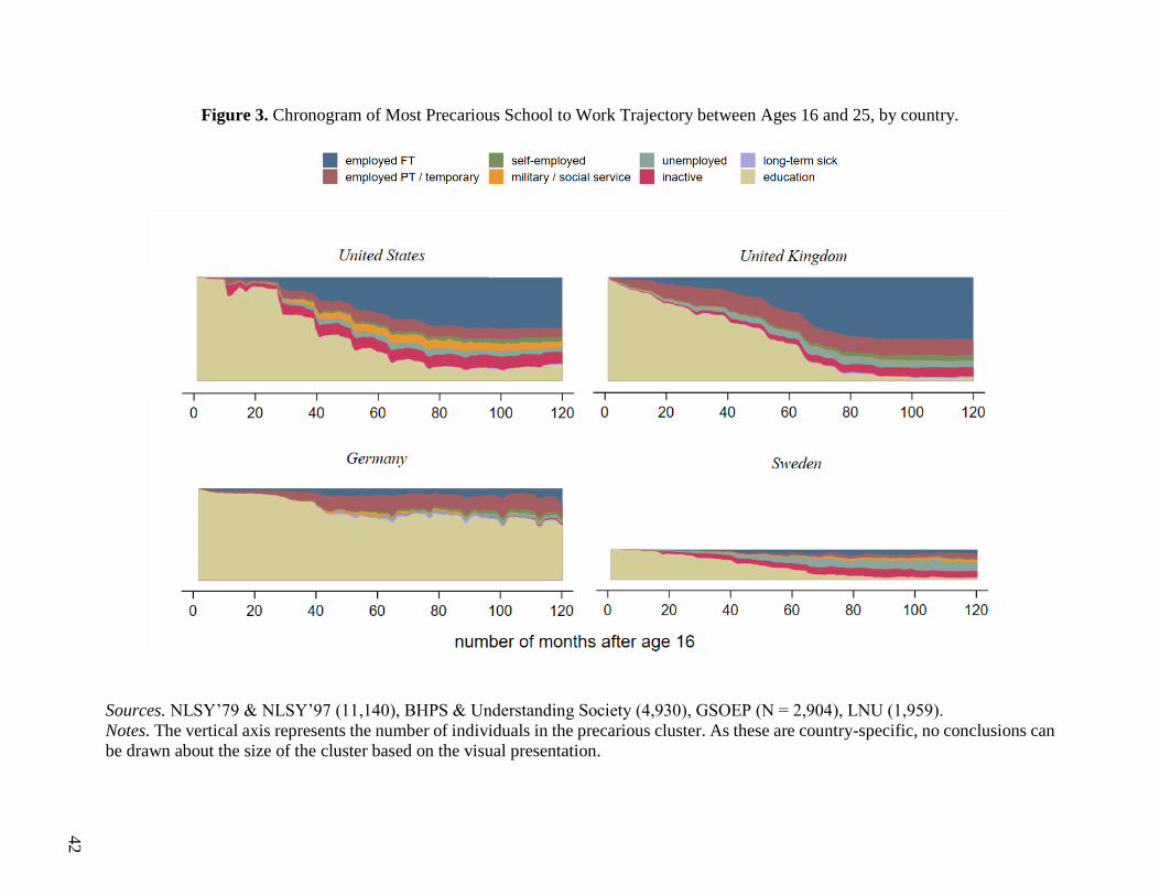
42

Figure 3. Chronogram of Most Precarious School to Work Trajectory between Ages 16 and 25, by country.


Notes. The vertical axis represents the number of individuals in the precarious cluster. As these are country-specific, no conclusions can

be drawn about the size of the cluster based on the visual presentation.

43

Another important feature of a precarious trajectory rather than a precarious position is the

number of spells that occur within the entire 120-month observed career. The more spells, the more

transitions in and out of states, and thus the more volatile (and presumably insecure) the labor

market entry phase. Table 4 documents these measures, as well as relevant distributions within the

most precarious trajectory and the other pathways. As seen in the second row, the precarious

trajectory for each country consists of more spells than the alternatives; about 1 to 1.5

(significantly) more spells in the United Kingdom and Germany, and only 0.3 more spells in

Sweden. Strikingly, precarious careers in the United States contain a much higher number of spells

than the other countries: 11.1 (vs. 4 to 6). Although the ‘other’ pathways in the US early labor

market are also much more unstable (6.2 spells), the precarious cluster has almost twice as many

transitions in the first ten years of the career.

Change over time

Are school-to-work trajectories becoming more vulnerable and precarious over time? To

answer this question, a series of nested logistic regressions were applied to the identified cluster

distribution (Tables 5 thru 8). The dependent outcome is defined as precarious (1) vs. not

precarious (0), and the estimates are odds ratios. Model 1 consists of just a dummy for the most

recent decade of birth cohorts (1980s), whereby the reference category is 1970s or 1960s (United

States). Models 2 and 3 add highest educational attainment, gender, race/ethnicity, and nativity.

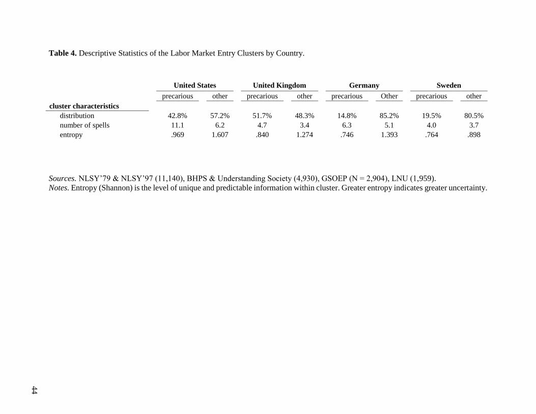
44

Table 4. Descriptive Statistics of the Labor Market Entry Clusters by Country.

United States United Kingdom Germany Sweden precarious other precarious other precarious Other precarious other

cluster characteristics

distribution 42.8% 57.2% 51.7% 48.3% 14.8% 85.2% 19.5% 80.5% number of spells 11.1 6.2 4.7 3.4 6.3 5.1 4.0 3.7 entropy .969 1.607 .840 1.274 .746 1.393 .764 .898


Notes. Entropy (Shannon) is the level of unique and predictable information within cluster. Greater entropy indicates greater uncertainty.

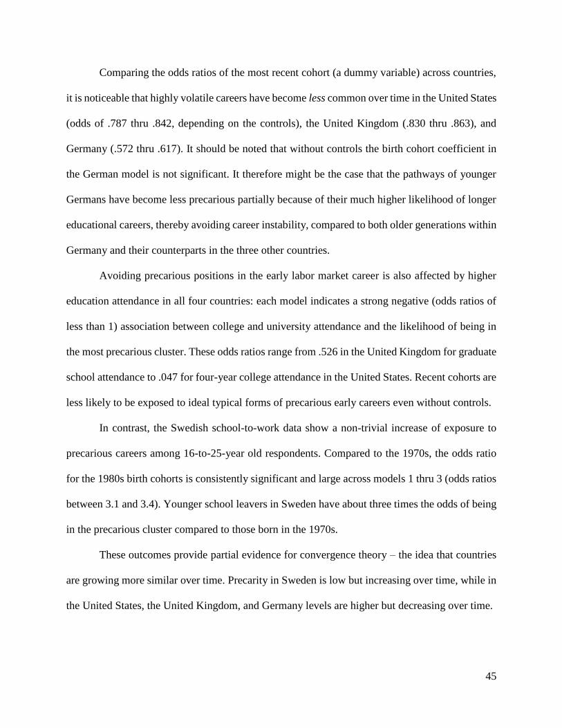
45

Comparing the odds ratios of the most recent cohort (a dummy variable) across countries,

it is noticeable that highly volatile careers have become less common over time in the United States

(odds of .787 thru .842, depending on the controls), the United Kingdom (.830 thru .863), and

Germany (.572 thru .617). It should be noted that without controls the birth cohort coefficient in

the German model is not significant. It therefore might be the case that the pathways of younger

Germans have become less precarious partially because of their much higher likelihood of longer

educational careers, thereby avoiding career instability, compared to both older generations within

Germany and their counterparts in the three other countries.

Avoiding precarious positions in the early labor market career is also affected by higher

education attendance in all four countries: each model indicates a strong negative (odds ratios of

less than 1) association between college and university attendance and the likelihood of being in

the most precarious cluster. These odds ratios range from .526 in the United Kingdom for graduate

school attendance to .047 for four-year college attendance in the United States. Recent cohorts are

less likely to be exposed to ideal typical forms of precarious early careers even without controls.

In contrast, the Swedish school-to-work data show a non-trivial increase of exposure to

precarious careers among 16-to-25-year old respondents. Compared to the 1970s, the odds ratio

for the 1980s birth cohorts is consistently significant and large across models 1 thru 3 (odds ratios

between 3.1 and 3.4). Younger school leavers in Sweden have about three times the odds of being

in the precarious cluster compared to those born in the 1970s.

These outcomes provide partial evidence for convergence theory – the idea that countries

are growing more similar over time. Precarity in Sweden is low but increasing over time, while in

the United States, the United Kingdom, and Germany levels are higher but decreasing over time.

46

Table 5. Logistic Regression on Most Precarious Labor Market Entry Cluster: United States.

model 1 model 2 model 3

Β s.e. β s.e. β s.e.

birth cohort (ref=1960s)

1980s .842** .050 .787** .061 .793** .065

education age 25 (ref=AA or less)

BA .047*** .004 .048*** .004 post-graduate .015*** .004 .015*** .004

gender

female 1.007 .067 .998 .067

race / ethnicity (ref=white)

black 1.220* .099 Hispanic 1.052 .105 Asian 1.121 .278 other 1.236 .363

nativity (ref=no immigrant background)

1st generation .843 .152 2nd generation .769 .148

constant .845 .042 2.414 .188 2.337 .200

summary statistics

N 5,702 5,702 5,702

R2 .001 .299 .300

Wald Chi2 > prob. .004 .000 .000

Sources. NLSY’79 & NLSY’97. N = 11,140. Notes. Sampling weights applied. Significance: * = p <.05, ** = p < .01, *** = p < .001.

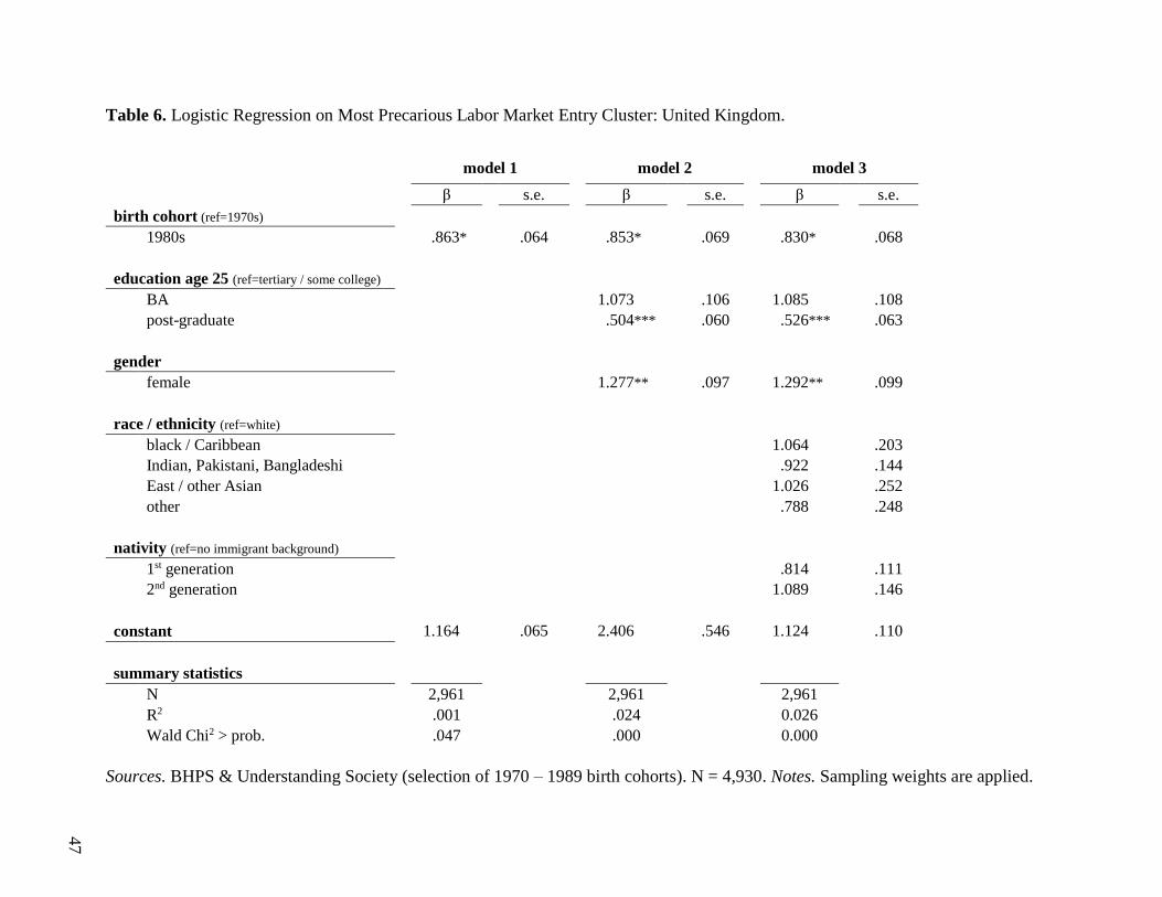
47

Table 6. Logistic Regression on Most Precarious Labor Market Entry Cluster: United Kingdom.


β s.e. β s.e. β s.e.


1980s .863* .064 .853* .069 .830* .068

education age 25 (ref=tertiary / some college)

BA 1.073 .106 1.085 .108 post-graduate .504*** .060 .526*** .063

gender

female 1.277** .097 1.292** .099

race / ethnicity (ref=white)

black / Caribbean 1.064 .203 Indian, Pakistani, Bangladeshi .922 .144 East / other Asian 1.026 .252 other .788 .248


1st generation .814 .111 2nd generation 1.089 .146

constant 1.164 .065 2.406 .546 1.124 .110

summary statistics

N 2,961 2,961 2,961

R2 .001 .024 0.026

Wald Chi2 > prob. .047 .000 0.000

Sources. BHPS & Understanding Society (selection of 1970 – 1989 birth cohorts). N = 4,930. Notes. Sampling weights are applied.

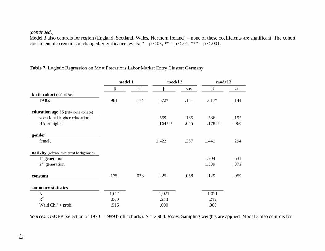
48

(continued.)

Model 3 also controls for region (England, Scotland, Wales, Northern Ireland) – none of these coefficients are significant. The cohort

coefficient also remains unchanged. Significance levels: * = p <.05, ** = p < .01, *** = p < .001.

Table 7. Logistic Regression on Most Precarious Labor Market Entry Cluster: Germany.

model 1 model 2 model 3 β s.e. β s.e. β s.e.


1980s .981 .174 .572* .131 .617* .144

education age 25 (ref=some college)

vocational higher education .559 .185 .586 .195 BA or higher .164*** .055 .178*** .060

gender

female 1.422 .287 1.441 .294


1st generation 1.704 .631 2nd generation 1.539 .372

constant .175 .023 .225 .058 .129 .059

summary statistics

N 1,021 1,021 1,021

R2 .000 .213 .219

Wald Chi2 > prob. .916 .000 .000

Sources. GSOEP (selection of 1970 – 1989 birth cohorts). N = 2,904. Notes. Sampling weights are applied. Model 3 also controls for

49

(continued.)

region (West Germany and (former) East Germany) – this dummy variable is not significant. The cohort coefficient also remains

unchanged. Significance levels: * = p <.05, ** = p < .01, *** = p < .001.

Table 8. Logistic Regression on Most Precarious Labor Market Entry Cluster: Sweden.


β s.e. β s.e. β s.e.


1980s 3.148*** .649 3.251*** .701 3.489*** .773

education age 25 (ref=2-year degree / some college)

BA .492** .121 .482** .119 MA+ .355** .112 .345** .110

gender

female 1.421 .294 1.434 .298


1st generation .818 .275 2nd generation 1.894 .620

constant .127 .021 .143 .036 .131 .033

summary statistics

N 688 688 688

R2 .049 .086 .092

Wald Chi2 > prob. .000 .000 .000

Sources. LNU (sel. 1970 – 1989 cohorts). N = 1,959. Notes. Sampling weights applied. Sig.: * = p <.05, ** = p < .01, *** = p < .001.

50

Exposure to precarious careers

The assessments on changing school-to-work trajectories over time in Tables 5 thru 8 also contain

relevant associations between demographics and likelihood of being in the most precarious cluster.

As mentioned before, college or university attendance is highly protective for the early career. In

each of the countries’ series of predictive models, the odds ratios of the higher levels of education

indicate a significantly lower likelihood of experiencing a precarious school-to-work trajectory.

This protection is visible for the bachelor’s degree vis-à-vis secondary education or some college

in the United States, Germany, and Sweden. For school leavers in the United Kingdom only an

MA or higher indicates protection.

After adjusting for these protective effects of education, gender is not associated with a

higher or lower chance of entering a precarious early career in the United States, Germany, or

Sweden.3 However, women in the United Kingdom are significantly more likely than men to be

part of this precarious cluster (an odds ratio of 1.277), even after controlling for other

demographics in Model 3. Importantly, the interaction between gender and children was predictive

of selection into more less precarious trajectories in the United Kingdom, Germany, and Sweden.

In contrast, women with (young) children in the United States are about 2.6 times more likely to

be tracked into a precarious early career compared to men with young children, and 2.45 times

more likely compared to women with no children. These interactions are not shown in the tables.

There is a mixed picture of the exposure of racial and ethnic minorities to precarious early

careers. The German and Swedish data do not indicate strong disadvantages for minorities as

measured by (family) immigrant backgrounds. Furthermore, no statistical disadvantages regarding

3 Appendix B documents the unadjusted proportions between the precarious cluster and the other clusters, indicating

that women are overrepresented in precarious careers in the United States and Sweden.

51

race/ethnicity and immigrant background (1st and 2nd generations) are apparent in the predictive

models for the United Kingdom, despite sizable bivariate disparities between whites and South

Asians in the descriptive statistics (Appendix B). However, the estimates of the odds of entering

the most vulnerable school-to-work pathway in the United States (OR = 1.22) indicates a much

higher exposure for Blacks (mostly African-Americans). This strong disadvantage cannot be

attributed to inequality within education and therefore partially indicates the consequences of labor

market discrimination.

Discussion

Theoretical frameworks describe the structural components of modern transitions from formal

education to the labor market, better understood as the school-to-work trajectory. The idea that the

educational system operates equally (meritocratically) across countries (Wilensky, 1975) is

outdated. Furthermore, scholars have suggested that regime types predict varying degrees of public

investment in secondary and tertiary education across countries (Willemse & De Beer, 2012).

Other sociological and economic research concentrates on either the moment of labor market entry

or the early career outcomes. This study is an attempt to explore harmonized longitudinal data

from different wealthy nations and to assess whether the variation in pathways can supplement

welfare state research and school-to-work transition research.

The exploratory character of the analysis is partially a function of the selected methods.

The modern school-to-work transition has become increasingly complex in post-industrial

countries because of lengthier educational careers and the additional overlap with other life course

52

events. The image of a young individual completing his or her education and then entering a

profession after graduation no longer holds. Instead, the youngest generations of school leavers

string together complex spells, sometimes in education, other times at work, at home, or

unemployed, regardless of having graduated. Sequence analysis is well suited to examine the

pathway from school to work holistically and to reveal the inequalities within some of them; the

least desirable combinations of instability, precarious work, and inactivity.

The descriptive statistics of 1960s, 1970s, and 1980s birth cohorts – entering the labor

market between the late 1970s and the 2000s in four different countries – largely confirmed the

structural features of the school-to-work transition as expected from welfare state research and

labor market research. The US educational expansion occurred much earlier than the three

European countries. However, the time spent in full-time education in United Kingdom, Sweden,

and Germany have gradually surpassed the United States. By comparing the cumulative

enrollments between age 16 and age 25 for different birth cohorts, the dramatic increase of

educational attainment of Germany.

Using cross-national harmonized month-to-month data that consist of lengthy observations

(age 16 to 25) is an improvement on earlier comparative studies the school-to-work transitions.

This approach enabled us to observe features of welfare state regimes in the ideal-typical pathways

from high school to adulthood across the four countries. If de-commodification – through a

combination of labor market policies – leads to a higher prevalence of safe (full-time) employment,

fewer spells and less moving from employment to non-employment, and a lower chance of

temporary work, we should conclude that careers in social-democratic and corporatist countries

are the most stable and least precarious. Ideal-typical school-to-work trajectories are most volatile

53

in the United States, followed by the United Kingdom, and much more stable in Germany and

Sweden.

In addition, de-commodification that operates through universalistic social security

policies and public goods – including education – should affect school leavers’ ability to ‘escape’

from vulnerable labor market spells, for instance by reenrolling in college. My analyses also

confirmed these expectations derived from welfare state literature. Patterns of moving in and out

of temporary work, part-time work, and self-employment contribute dramatically to insecurity in

the school-to-work pathway for American youths. Importantly, transitioning between education

and full-time employment is much more common in the early careers in Sweden and Germany,

indicating a tighter job-match compared to the other two countries. These findings can also be

understood from a labor market theory perspective. Occupational labor markets, such as Germany

and Sweden, have a stronger linkage between educational degrees and jobs which facilitates a

faster entry into stable employment (Bol and Van de Werfhorst 2011, Brzinsky-Fay 2007).

When concentrating on the most vulnerable school-to-work trajectories in each of the four

countries the different experiences of young school leavers becomes even sharper. About half of

British and American youths experience what I call precarious early careers, compared to only

15 to 20 percent in Germany and Sweden. What is labeled as an ideal-typical precarious career

varies a bit across countries; some are more based on instability, others on more exposure to

unemployment cycles. However, the type of pathway that was identified as least vulnerable in the

United States was still more precarious in terms of instability and exposure to temporary work than

the most precarious clusters in Germany and Sweden. This illustrates the extreme differences

between countries during the early career phase, as well as a likely underestimation of the

54

difficulties that young Americans face. Chapter 3 of this dissertation examines precarious early

careers as concept in much greater detail.

Two important new findings regarding the stratification within the pathways from school

to work come from this study. First, a comparison of the 1960s/1970s birth cohorts and the younger

1980s cohort suggests that pathways from school to work have become slightly less precarious

over time in two liberal regime countries: the United States and the United Kingdom. Educational

expansion at itself could have affected younger generations’ lower chance of exposure to

precarious labor market positions, but the lower odds remained significant after adjusting for

higher educational attendance. Conversely, more recent school leavers in Sweden seem more

likely to be exposed to precarious early careers. Keeping in mind the sharp differences across

countries’ school-to-work trajectories, these changes over time suggest some convergence between

the liberal-regime countries and the social-democratic case.

Second, higher education attendance and completion are strongly protective of selection

into the precarious pathways to the labor market in all four countries. When adjusted for this effect,

a few more inequalities came to the fore. Women tend to be more exposed to precarious pathways

than men, although this association only held in the regression analysis of the British data. More

research is needed to unpack these gender differences within and across countries. Finally, Black

Americans in United States are structurally disadvantaged in comparison to whites as they are

significantly more likely to experience precarity in the labor market.

The next three chapters will further unpack the cross-national differences of the complexity

in the school-to-work trajectory, such the macro-economic factors associated with (early) labor

market entry, patterns of educational reenrollment, and precarious early careers.

55

Chapter 2.

Encouraged or Discouraged? How do Economic Conditions Shape Student

Early School Leaving and Young Workers’ Reenrollment? An Analysis of the

US, the UK, Germany, and Sweden.

Introduction

Early school leaving has been of interest to international comparative researchers, increasing our

understanding of how different educational systems vary in terms of average school leaving age,

secondary education attrition rate, and higher education attrition rate (Rumberger, 2001).

Numerous studies have also emphasized the sociological forces behind the unequal educational

attainment outcomes across social, economic, and ethno-racial background groups – the so-called

primary effects on educational outcomes (Boudon, 1974). This body of research also includes

cross-national studies on the primary effects within countries (see Shavit & Blossfeld, 1993).

Furthermore, the complimentary secondary effects have received considerable attention in the

sociology of education (see Breen, Luijkx, Muller & Pollak, 2009). Secondary effects refer to

students of the same educational achievement and performance levels making different educational

decisions depending on their social background.

Both primary and secondary effects have also been studied in the context of the school-to-

work transition – the life phase in which students leave the educational system for the first time.

Several recent empirical studies concentrate on the social background factors that contribute to,

56

for instance, delayed entry into college (Goldrick-Rab & Han 2011, Rowan-Kenyon 2007) and

‘stop-out patterns’ in higher education (Desjardins, Ahlburg & McCall, 2006). These topics have

become of greater interest to sociologist of education as the complexity of school leaving and

reenrollment have become more prevalent in the life phases young adults. Together, this body of

literature has led to a better understanding of educational reentry after the first labor market entry,

including individual-level motivations and the opportunities and constraints associated with

returning to education.

Compared to these individual- and social context mechanisms, the influence of macro-

economic factors on both school leaving and reenrollment has been of less concern to sociologists

and educational researchers. Furthermore, much of our theoretical understanding of how macro-

economic factors shape the current trends of school leaving and enrollment is still based on

economic theory only (e.g. Becker, 1964). As discussed below, this framework assumes that

individuals – students, families, and school leavers – are rational actors who maximize the balance

between the costs of attending education and the monetary benefit of labor market returns.

Economists therefore assume that a recessionary economy – with a higher level of unemployment

– makes staying in school longer (to avoid unemployment) and returning to school (to increase

human capital) the most ‘rational’ choices compared to more stable economic circumstances. The

aggregate rates of early school leaving (going down during a recession) and reenrollment (going

up during a recession), as has been observed in the United States (Barr & Turner 2013), give no

reason to question this interpretation of economic theory.

Based on these influential theoretical ideas and aggregate statistics, I originally meant to

compare the extent to which the Great Recession (2007 – 2009) affected school leaving and

reenrollment in different countries, and whether these macro conditions have explanatory power

57

over and above the social and educational stratification factors that operate at the individual level.

In addition, given the strong and structural cross-national differences in the organization of the

school-to-work transition, I also intended to measure whether (and why) countries vary in the

extent to which more recent cohorts stay in school longer and reenroll more frequently.

However, the results revealed an unexpected trend for the United States vis-à-vis the

United Kingdom, Germany, and Sweden. Contrary to a human capital theory hypothesis, the

analyses in this chapter show that poor macro-economic conditions in the United Stated tend to

make lower-educated students more likely to leave the educational system early, while

simultaneously making lower-educated school leavers less likely to reenter the educational system.

This chapter starts with a discussion of a relatively small body of research on macro-

economic triggers of early school leaving and educational reenrollment. This review will indicate

that empirical research on this topic is often focused on aggregates (rather than individual

outcomes), is rather limited in its scope (time observations, countries), and is also inconclusive

about the mechanisms behind the few findings that contradict human capital theory. The empirical

contribution of this chapter relies on longitudinal data from four different countries with distinct

school-to-work transitions: United States, United Kingdom, Germany, and Sweden. The major

cross-national and cross-cohort differences of school leaving and reenrollment will be discussed

first, as originally planned. Subsequently, survival analysis models will be applied to the school-

to-work career trajectories to answer the question: How do macro-economic conditions such as

labor market fluctuations and recessions affect students’ school leaving pace and school leavers’

reenrollment probability?

58

Macro-Economic Factors

Early school leaving

Explanations for the variation in school leaving age across countries have been documented in

numerous international studies (e.g. Lamb & Markussen, 2011; Lavrijsen, 2015). This literature is

reviewed in Chapter 1 of this dissertation.

A small body of mostly European research groups has investigated the impact of macro-

economic forces and social context variables on (early) school leaving. Their research is based on

the idea that socio-economic contexts shape the individual-level decision-making as known from

micro-economics’ theorization of school choices (Cabus & De Witte, 2016). In the framework of

Human Capital Theory, a students’ decision to stay or leave school is always based on the net

outcome of weighing the direct costs of education, the indirect costs of education (opportunity

costs of time), and the expected future benefits (productivity and wages) (Becker, 1962).

Previous research has suggested three important context factors that could affect the

balance between the costs and benefits for students. First, labor market characteristics may

influence the school enrollment decisions of students. The unemployment rate is an indirect but

strong indication shaping expectations of future employment chances and wages. On the one hand,

scholars have suggested that an increasing (or high) unemployment rate triggers a so called

‘discouraged student’ effect. If students observe a large proportion of the current labor force being

unemployed, while holding higher level degrees, they could perceive their own current investment

in such qualifications as less valuable (compared to a labor market with a lower unemployment

rate). Researchers found some evidence for such a pattern in the United Kingdom (Tumino &

Taylor, 2015) and Spain (Petrongolo & San Segundo, 2002).

59

On the other hand, if higher-educated members of the workforce do better regardless of

rising unemployment, this may lead to the opposite estimation of students’ current investment –

one that makes staying in school more valuable, ceritus paribus. This expected positive

relationship between higher unemployment and lower rates of early-school leaving can be called

a ‘encouraged student effect’ and has been found by Clark (2011) who used panel data from

England. This study therefore seems to contradict the later discouraged student finding by Tumino

and Taylor (2013), that relies on similar data. Only one known study has used US data to take on

this question. Based on the National Longitudinal Survey of Youth 1979, Card and Lemieux

(2001) argue that higher unemployment rates partially explain the rise of US high school

completion rates in the 1970s.

Second, Cabus and de Witte (2012) have raised the possibility of a (direct) effect of the

macro-economic growth on early-school leaving fluctuations, independent of the impact of

indicators of employment chances (the unemployment rate). They point to research by Asteriou

and Agiomirgianakis (2001) who found a positive correlation between rising macro-economic

growth (GDP) and the secondary education enrollment rate in Greece. A more precise

measurement of the economic growth effect was conducted by Cabus and de Witte (2016) on

Dutch vocational education data, arguing that GDP growth significantly reduced the early school

leaving rate. Thus, both studies taking economic growth as the macro predictor point in the

direction of an encouraged student effect. Although these studies in economics imply early school

leaving variation to be affected by the economy being in recessionary vs. non-recessionary state,

they have only tested the GDP-change as the key independent variable.

Third, structural welfare state and labor market policies may attenuate the impact of macro-

economic context effects on early school leaving, yet empirical evidence on this is also scarce. For

60

instance, the generosity of the unemployment insurance system could play a role in individuals’

post-education returns, thereby reducing both the possible discouraged student and encouraged

student effects (De Witte et al., 2013). Furthermore, some economists have suggested that changes

to the minimum wage influence the early school leaving rates, but empirical research has resulted

in contradicting directions of this association. Montmarquette, Viennot-Briot and Degenais (2007)

state that a higher minimum wage leads to more dropout because of students’ lower (relative) wage

gain from further education. Pedace and Rohn (2011) argue that a higher minimum wage increases

unemployment for early school-leavers, thereby reducing the incentive to leave school earlier than

anticipated. However, more comprehensive empirical studies find no effect of minimum wage

policy on attrition or retention rates (e.g. Crofton, Anderson & Rawe, 2009; Warren & Hamrock,

2010).

Reenrollment: labor market experience

Once transitioned from school to work, which factors contribute to educational reenrollment? The

rationality assumption of human capital theory predicts that instant economic dislocation, such as

job loss, is the most straightforward market-related force that would encourage young individuals

to reenroll. This ‘needs-and-resource’ perspective explains how individuals reentering education

are often motivated by updating their job skills in response to their deteriorating position in the

labor market (Setftersten & Lovegreen, 1998). Signs of these ad hoc work- and education-

decisions have been found in different forms (Kerckhoff, 1996). Net of other effects, researchers

found individuals responding to unstable careers (Elman & O’Rand, 2007), perceived job

insecurity (Elman & O’Rand 2002; Smart & Pascarella, 1987), and a recent lay-off (Ghilani, 2008;

Knapp & Harms, 2002). In NLSY’79 data, Mroz and Savage (2006) find that if confronted with

61

unemployment at a young age, individuals are more likely to reenroll in education. This is a so-

called ‘human capital catch-up response’.

However, this educational ‘refreshing’ is not limited to individuals who experience

unemployment or instability. Workers are also responding to their relative position in the labor

market. That is, relative to equally educated groups, mismatched workers – whose pay or job duties

are low given their educational attainment – tend to feel dissatisfied and may therefore seek

educational updates to improve their position (DiPrete, 1993). Interview data show this dynamic.

Improving one’s employment position is the most important argument in favor of returning to

college (Deterding, 2015) in a recent survey among 25-34-year-olds. These respondents also

supported a narrative of upward social mobility, which illustrates the tight link between economic

imperatives and the symbolic value of education.

In addition to adverse conditions, ‘good jobs’ can also provide incentives for reenrollment.

This perspective, which is not often applied, suggests that above-average employed workers are

more likely to leave the labor market temporarily for an additional credential – e.g. a BA for AA

graduates or an MBA for BA graduates. It is important to note that the same human capital

rationality – maximizing post-education pay-off – also explains this effect. Moreover, some jobs

at the higher end of the occupational spectrum are also more likely to provide opportunities to

return to school as they tend to have more flexible work hours (Kasworm, 2003).

Clark (1960, 1980) proposed the ‘cooling-out hypothesis,’ suggesting that individuals act

rationally by downwardly adjusting their educational goals after a first-hand (unsuccessful) college

experience. Scholarly research is unsettled on this hypothesis as some studies find evidence for

lower-educated individuals and college dropouts being less likely to reenroll (Brint & Karabel,

1989; Dougherty, 1994; Pascarella, Edison, Nora, Hagedorn & Terenzini, 1998), while others have

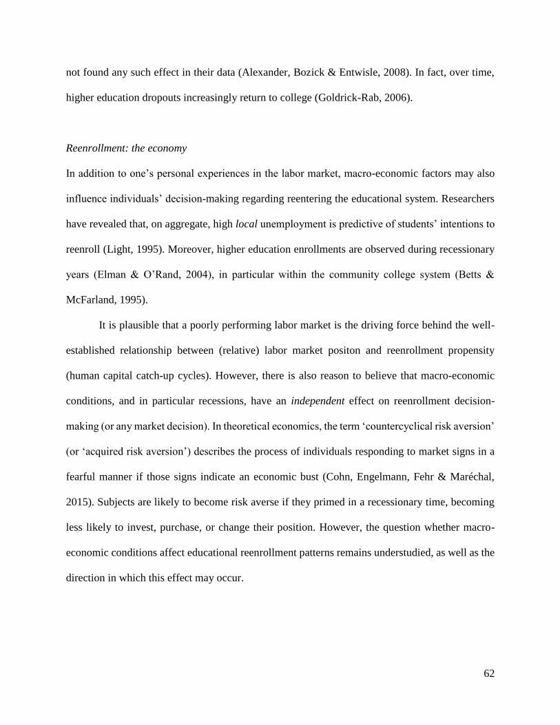
62

not found any such effect in their data (Alexander, Bozick & Entwisle, 2008). In fact, over time,

higher education dropouts increasingly return to college (Goldrick-Rab, 2006).

Reenrollment: the economy

In addition to one’s personal experiences in the labor market, macro-economic factors may also

influence individuals’ decision-making regarding reentering the educational system. Researchers

have revealed that, on aggregate, high local unemployment is predictive of students’ intentions to

reenroll (Light, 1995). Moreover, higher education enrollments are observed during recessionary

years (Elman & O’Rand, 2004), in particular within the community college system (Betts &

McFarland, 1995).

It is plausible that a poorly performing labor market is the driving force behind the well-

established relationship between (relative) labor market positon and reenrollment propensity

(human capital catch-up cycles). However, there is also reason to believe that macro-economic

conditions, and in particular recessions, have an independent effect on reenrollment decision-

making (or any market decision). In theoretical economics, the term ‘countercyclical risk aversion’

(or ‘acquired risk aversion’) describes the process of individuals responding to market signs in a

fearful manner if those signs indicate an economic bust (Cohn, Engelmann, Fehr & Maréchal,

2015). Subjects are likely to become risk averse if they primed in a recessionary time, becoming

less likely to invest, purchase, or change their position. However, the question whether macro-

economic conditions affect educational reenrollment patterns remains understudied, as well as the

direction in which this effect may occur.

63

Analytical Strategy

The empirical section of this paper is focused on two key dependent variables: (1) the probability

of school leaving among students who never previously entered the labor market, and (2) the

probability of educational reenrollment among school leavers.

Regarding the former, the literature is ambiguous about the impact of macro-economic

conditions on early school leaving. Are students discouraged or encouraged to stay in the

educational system? In first empirical section, the analysis will estimate the association between

social backgrounds – primarily gender, race, ethnicity, and nativity – and the ‘survival probability’

in the educational system. Its findings should largely confirm existing knowledge about social

inequality of educational attainment. Hence, the discussion will be focused on the cross-national

differences.

Of key importance is the association between the state of the macro-economy during the

critical phase of a student’s educational career and the probability of early or late school-to-labor

force transition. The independent variable here is concerned with the macro-economic signs to

students, rather than fluctuations in unemployment rates or GDP growth. The main predictor of

interest is a dummy variable measuring no recession (0) vs. recession (1) while enrolled in school.

Compared to earlier studies, this official marker of the state of the economy therefore entails a

broader societal stimulus to students.

Macro stimuli may operate differently according to the educational level. My analyses are

therefore conducted on two groups of students: high school students who never entered the labor

market and college students (BA or equivalent) who never entered the labor market. These two

types of students are also reasonably comparable across countries. Students enrolled in country-

64

specific post-secondary / non-BA programs are excluded. The state of the economy is measured

during high school (between ages 14 and 16) for secondary education survival and during college

(first year) for higher education survival. These analyses will adjust for all individual-level

variables available and therefore be net of variation in school leaving pace between social groups.

The analysis for the second research question, regarding educational reenrollment, has a

rather similar framework. Conditional on having left day-time (full-time) education for the

first time, what is impact of the unemployment rate and the state of the economy on

reenrollment probability? This part of the study is also organized as a survival (in the labor

market) analysis, while adjusting for all important individual-level variables. The analyses are

focused on two key predictor variables, both measured at the initial labor market entry: a dummy

for recession/non-recession and the unemployment rate. More specifically, the models will test

whether the unemployment rate at entry triggers a faster or slower educational reenrollment pace,

whether a recession at entry affects this probability, and whether it does so net of the unemployment

rate. The predictive models are split by educational level and focus on two groups that have most

to gain from educational reenrollment: high school dropouts and higher education dropouts.

Finally, the reenrollment hazard ratios will be estimated for different occupational groups.

Data

The data are drawn from large longitudinal datasets that capture the month-to-month positions in

education and in the labor market; from the compulsory school age thru the early work life of

individuals until age 25. The selected datasets also include several different birth cohorts (1960s

thru 1980s) which allows analyses of changes in the school leaving and reentry trajectories over

time.

65

The data sources are the same as used in the analyses of Chapter 1. For the United States,

the National Longitudinal Survey of Youth (NLSY), both 1979 and 1997 (Bureau of Labor

Statistics 2014, 2015). For the United Kingdom the British Household Panel Study (BHPS)

(Taylor, 2010) and Understanding Society (US) (University of Essex, 2017). For Germany the

Socio-Economic Panel (GSOEP) (Wagner, Frick & Schupp, 2007). For Sweden the Level of

Living Surveys or Levnadsnivåundersökningarna (LNU) (Stockholm Universitet, 2010).4

Methods

For survival in the educational system, the t-1 observation of each selected respondent is ‘enrolled

in full-time education’ in March of the year in which he or she turned 16 – a mid-semester month

to avoid the traditional Summer and Winter breaks. The length of observations is standardized at

120 months (months as the unit of analysis). Any first observed non-full-time education position

is defined as the event of interest: leaving day-time education for the first time. However, this

hiatus must be longer than seven months (more than one semester) to avoid students who were not

enrolled for just a few months. This conservative definition does therefore not capture the smallest

‘stopouts’ or longer breaks.

Conversely, time (‘survival’) in the labor market is measured in months and up to 120

months after initial labor market entry. Missing data within work biographies are due to

respondents who drop out of the study prematurely and do not return in any of the subsequent data

collection years. Hence, right-censoring is adjusted for in the predictive models.

4 To avoid redundancy between the Chapters, the Data section of this Chapter does not include the most detailed

description of the countries’ datasets used. The most elaborate introduction of the data are presented in Chapter 1.

66

The individual-level predictors and macro-economic predictors estimated in a Cox (1972)

proportional hazard regression model. Each j-th subject hazard of ‘school leaving’ or ‘educational

reentry’ – ℎ(𝑡|𝑋𝑗) – is found through:

ℎ(𝑡|𝑋𝑗) = ℎ0(𝑡) exp(𝑋𝑗𝛽𝑥) [2.1]

where ℎ0(𝑡) denotes the baseline hazard and 𝛽𝑥 denotes the regression coefficients as estimated

from the data.

Findings

School leaving structure

The combined characteristics of the educational system and level of educational attainment and

completion are reflected in the survival rates in the education. Figure 4 plots the Kaplan-Meier

survival estimates in education after age 16 for the United States, the United Kingdom, Germany,

and Sweden. These rates should be interpreted as the cumulative risk of transitioning from school

to the labor force, for the first time. The probability of the occurrence of this one-time event applies

to both high school or college students, depending on having enrolled into higher education

immediately after high school completion. It should be noted that the estimates are calculated

across all birth cohorts (1970 – 1989).

Not accounting for any individual variation or cohort, the normal age of first exposure to

the labor market is much younger in the United States and the United Kingdom. In these two

67

countries, about 50 percent and 40 percent, respectively, have left education around age 19 or 20

(the 40th month after t-1). Almost all US and UK respondents (98 percent) have left the educational

system at least once by age 25 (both curves virtually touch the x-axis at month 120). In contrast,

the shape of the curves of Germany and Sweden suggest a much later average age of leaving the

educational system. German high school students remain in education slightly longer, but the

pattern of school-to-work transition ‘risk’ is otherwise remarkably similar in comparison to

Sweden. Furthermore, the share of individuals that have left the educational system by age 25 is

noticeably lower compared to the United States and the United Kingdom – 87.9% (Germany) and

94% (Sweden).

However, the most important variation of survival rates between types of students is

determined by educational level – higher education attendance. To illustrate this structural

difference, Figure 5 plots separate survival estimates for students who did not enroll in higher

education and those who did (before age 25). These rates report the significant difference of

‘educational survival’ for just the United States, but a similar structure exists in the three other

countries. The analyses are restricted to two groups: high school attendees only and BA attendees

(or higher) only.5

5 To compare relevant levels or education between countries, respondents who attended post-secondary (higher)

education but not a BA program (or equivalent) were excluded from the analysis.

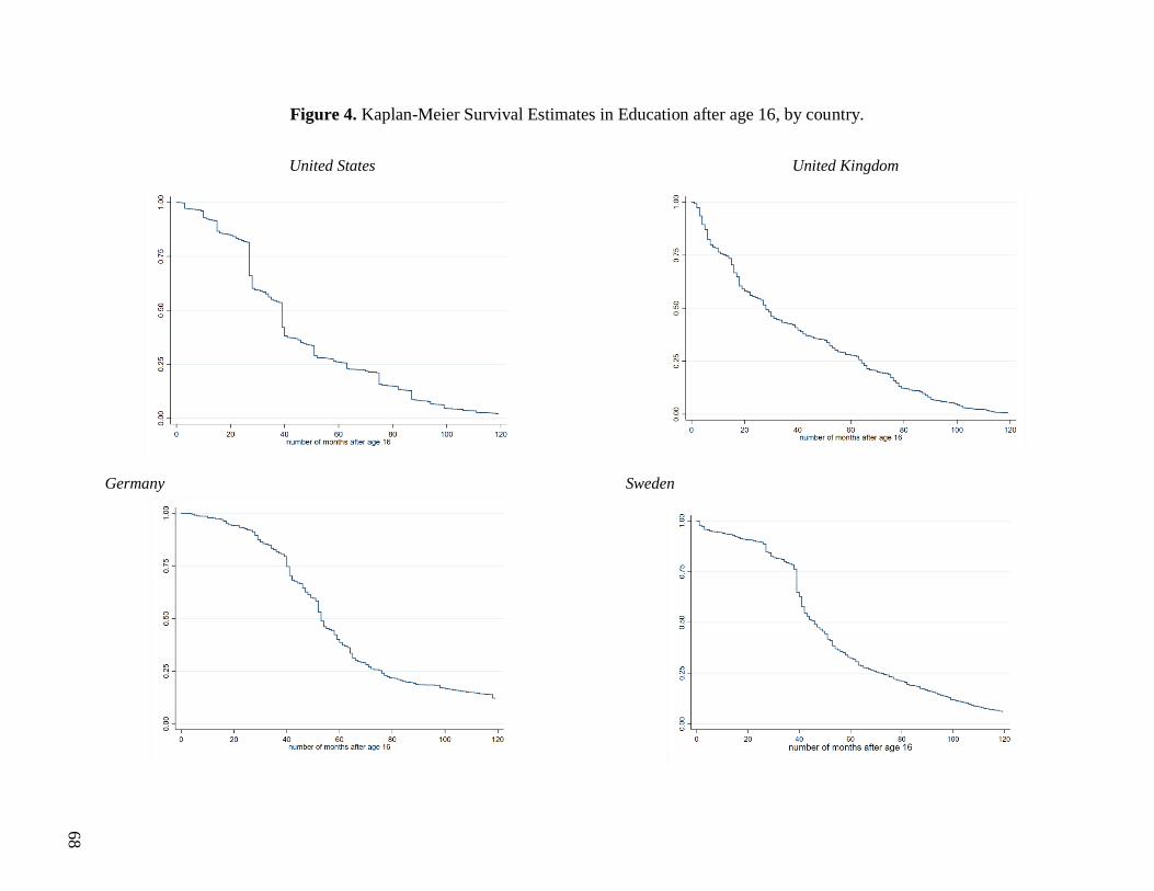
68

Figure 4. Kaplan-Meier Survival Estimates in Education after age 16, by country.


Germany Sweden

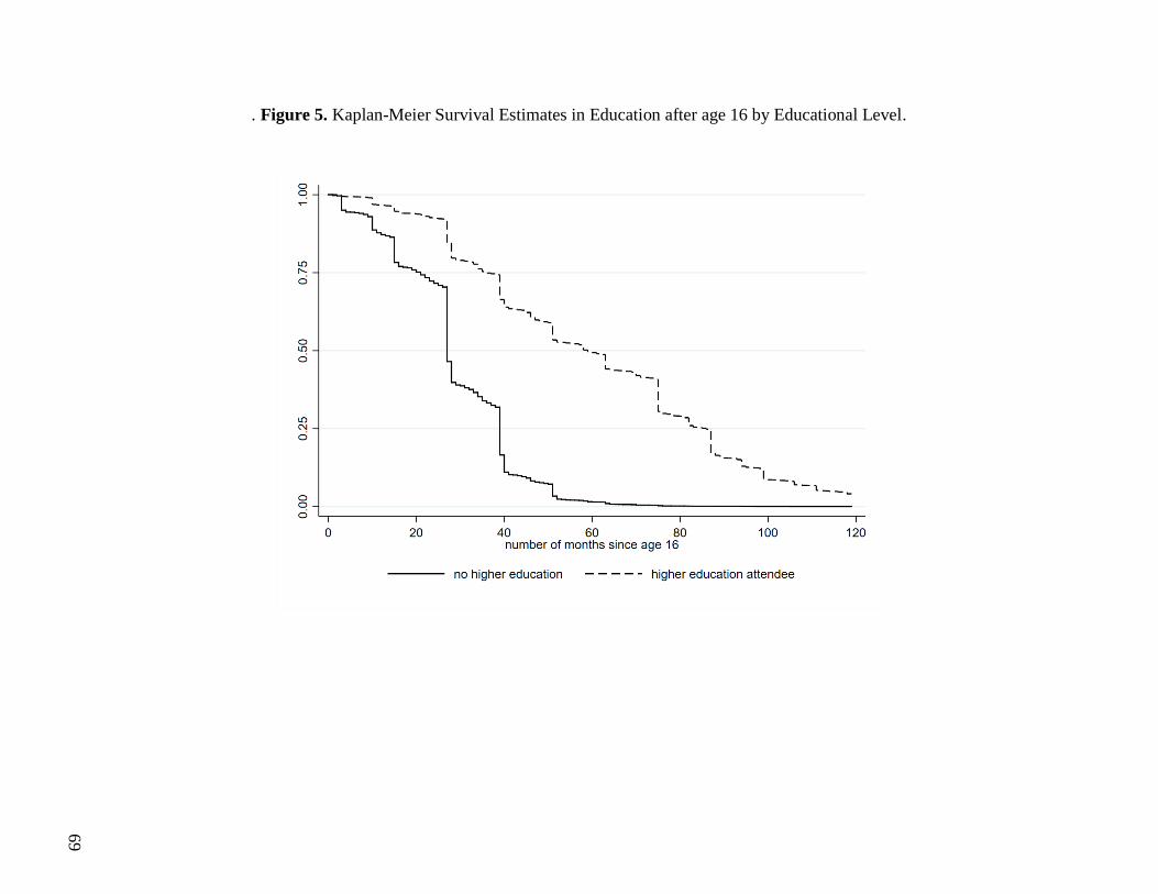
69

. Figure 5. Kaplan-Meier Survival Estimates in Education after age 16 by Educational Level.

70

Social background and early school leaving

Tables 1 thru 4 display nested models of hazard ratios of survival in the educational system for

high school attendees and bachelor’s degree attendees, separately, in each country. The focus is

on demographic backgrounds differentials in model 1, which are adjusted for highest education

obtained at age 25, as a measure of student grit and level, in model 2. In order to control for the

changes of educational enrollment characteristics over time, within countries, model 3 adjusts for

birth cohort (year).

The US data (Table 9) indicate a significantly higher risk of school leaving for women

among all subgroups (lower- and higher-education) and controlled for by all other covariates. The

hazard ratios range between 1.083 and 1.116. However, the sign of this hazard ratio does not

indicate a positive relationship in a model with no controls (not shown), suggesting that on average

women leave the educational system slower, but that its variation depends on race, ethnicity, and

immigrant background. Women display substantially higher retention rate across both educational

levels in Germany, also with no controls in the model. The proportional hazard ratios are also

substantial, ranging between .604 and .844 (Table 11).

On average, women leave the higher education system faster than men do across the ten-

year period between age 16 and age 25 in Sweden (Table 12). This significant gender effect among

bachelor’s degree attendees was also found in the British data, but only after adjusting for birth

cohort (Table 10, column 3); more recent cohorts are less likely to leave the educational system.

Some of these risk distributions are affected by childbearing.

An increased risk of school leaving across the two birth cohort decades for some ethno-

racial minorities is visible in the second panel of each Cox regressions table. Among US

respondents have not yet entered higher education (the first column), black (.794) and Hispanic

71

(.899) are significantly more likely to leave the educational system than whites. Black, Caribbean,

and South Asians in the UK display similar significant hazard ratios across all educational levels.

Net of these race- and ethnicity-effects in regression models for the United States and the United

Kingdom, first generation students have a lower survival probability in the United Kingdom (both

levels) and the United States (just BA level). Children of immigrants are also at higher risk of

entering the labor force at a younger age in the United Kingdom (Table 10).

The German and Swedish datasets only contain information on immigrant background.

Those largely consist of ethnic minorities. When controlled for gender, education attendance, and

birth cohort, these hazard ratios indicate somewhat surprising associations (model 3). The German

first- and second-generations are equally likely to remain in both secondary and tertiary education.

However, this categorization does not account for the German youth of Turkish origin, who do

typically display higher dropout chances (Kristen & Granato, 2007). There is also no observable

difference in survival probability for second generation students in Sweden. However, its first

generation – a mix of Persian immigrants and Finnish immigrants – leave the educational system

much faster than their counterparts with no immigrant background. As seen in model 3 of Table

12, the significant hazard ratios for this group are .474 (high school) and .581 (BA attendees).

The risk differentials of leaving school for different social groups should be interpreted

with some caution. First, we must assume that the facts that these models are split by educational

attendance and then controlled for by highest education in models 2 and 3 take away a substantial

amount of variation in survival rates. This approach suppresses the selection and sorting in the

educational system along demographic lines. Second, the event in these survival analyses is not

‘dropout’ but leaving for at least more than two semesters. Some individuals may return to the

educational system later on.

72

Table 9. Hazard Ratios of Leaving the Educational System for the First-Time among 16-year-olds, United States.


enrollment history by age 25: no higher

education BA-level

only no higher

education BA-level

only no higher

education BA-level

only

gender (ref=male)

female 1.093** 1.083* 1.116*** 1.084* 1.110*** 1.093*

race/ethnicity (ref=white)

black .829*** 1.109* .793*** 1.008 .794*** 1.000 Hispanic .940 1.033 .890** .919 .899** .917 Asian .929 .911 .960 .957 .928 .949 other .669** 1.133 .615*** 1.142 .656** 1.175


1st generation .986 .792* .921 .840* .912 .822* 2nd generation 1.088 1.057 1.111 1.075 1.027 1.028

education 1

HS / GED .573*** .573***

some college / AA 1.627*** 1.657*** BA

post-graduate .668*** .649***


1980s .812*** .859**

Sources. NLSY’79 (1962 – 1964 birth cohorts) & NLSY’97 (1980 – 1984 birth cohorts). N = 5,437 (no higher education). N = 3,446

(BA only).

Notes. Sampling weights are applied. 1 References: <HS (no higher education), BA (BA only). Significance levels: * = p <.05, ** = p <

.01, *** = p < .001.

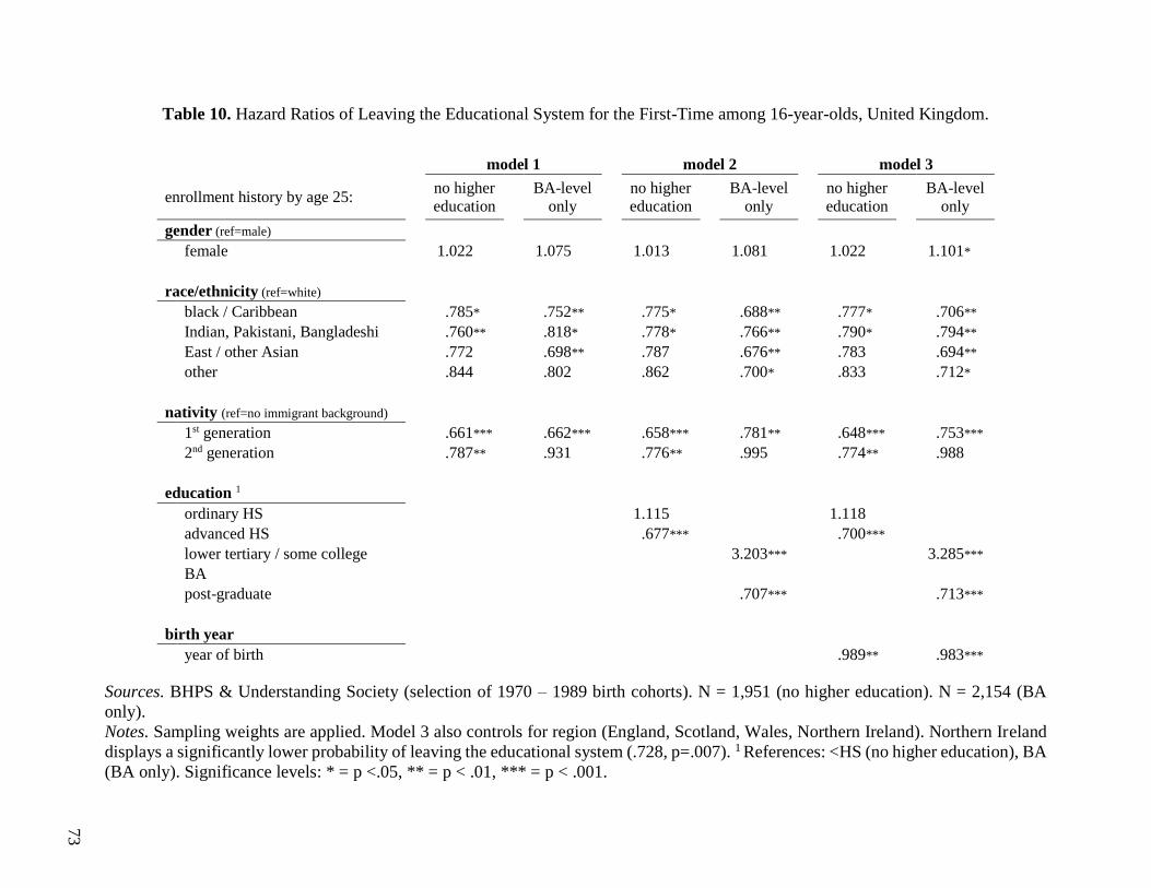
73

Table 10. Hazard Ratios of Leaving the Educational System for the First-Time among 16-year-olds, United Kingdom.



education BA-level

only no higher

education BA-level

only no higher

education BA-level

only

gender (ref=male)

female 1.022 1.075 1.013 1.081 1.022 1.101*

race/ethnicity (ref=white)

black / Caribbean .785* .752** .775* .688** .777* .706** Indian, Pakistani, Bangladeshi .760** .818* .778* .766** .790* .794** East / other Asian .772 .698** .787 .676** .783 .694** other .844 .802 .862 .700* .833 .712*


1st generation .661*** .662*** .658*** .781** .648*** .753*** 2nd generation .787** .931 .776** .995 .774** .988

education 1

ordinary HS 1.115 1.118

advanced HS .677*** .700***

lower tertiary / some college 3.203*** 3.285*** BA

post-graduate .707*** .713***

birth year

year of birth .989** .983***

Sources. BHPS & Understanding Society (selection of 1970 – 1989 birth cohorts). N = 1,951 (no higher education). N = 2,154 (BA

only).

Notes. Sampling weights are applied. Model 3 also controls for region (England, Scotland, Wales, Northern Ireland). Northern Ireland

displays a significantly lower probability of leaving the educational system (.728, p=.007). 1 References: <HS (no higher education), BA

(BA only). Significance levels: * = p <.05, ** = p < .01, *** = p < .001.

74

Table 11. Hazard Ratios of Leaving the Educational System for the First-Time among 16-year-olds, Germany.



education BA-level

only no higher

education BA-level

only no higher

education BA-level

only

gender

Female .811*** .604*** .844** .659*** .843** .660***


1st generation 1.062 .742 1.007 .874 .971 .874 2nd generation .968 1.013 .963 1.005 .911 .989

education 1

middle vocational HS .518*** .539***

HS / abitur .387*** .395***

some college, no degree .057*** .059***

vocational higher education 1.560 1.500

BA or higher

birth year

year of birth .976*** .993

Sources. GSOEP (selection of 1970 – 1989 birth cohorts). N = 1,715 (no higher education). N = 554 (BA only).

Notes. Sampling weights are applied. Model 3 also controls for region (West Germany and (former) East Germany) – this dummy

variable is not significant. 1 References: <HS (no higher education), BA or higher (BA only). Significance levels: * = p <.05, ** = p <

.01, *** = p < .001.

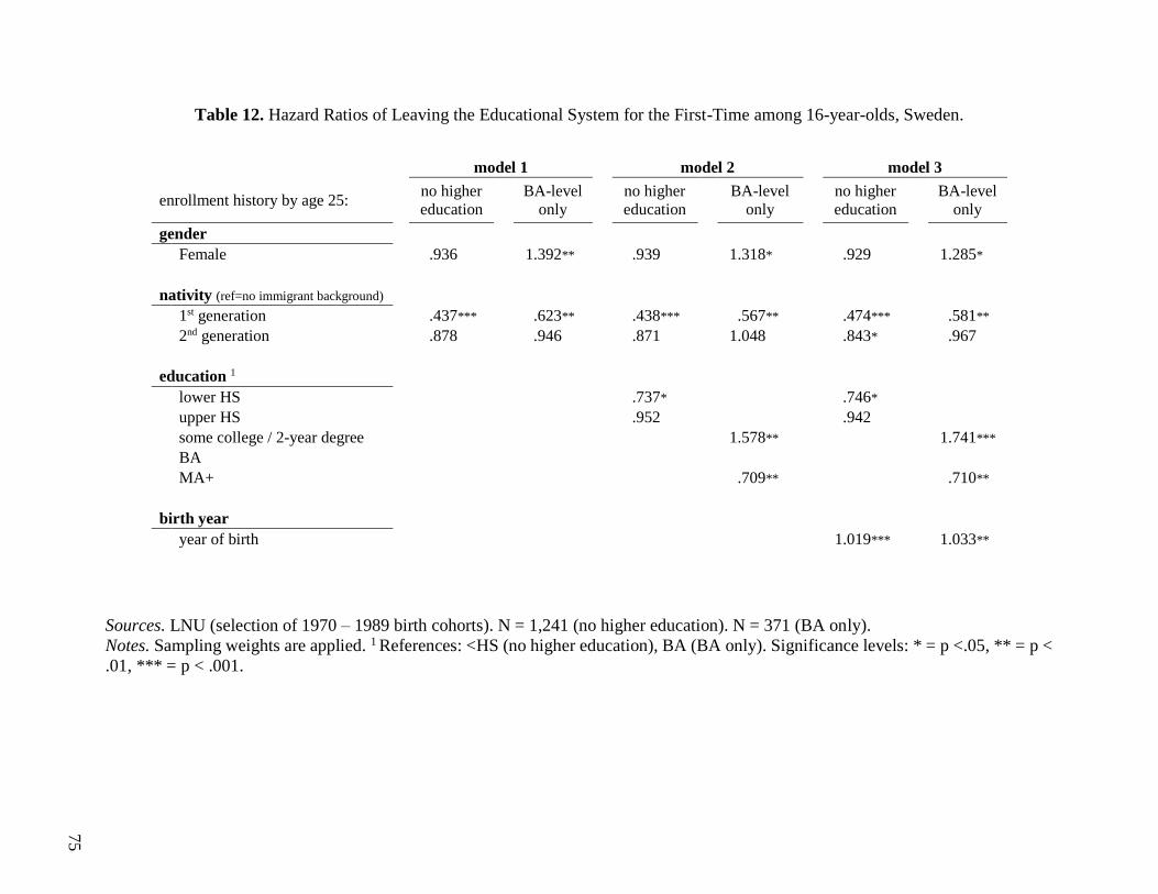
75

Table 12. Hazard Ratios of Leaving the Educational System for the First-Time among 16-year-olds, Sweden.



education BA-level

only no higher

education BA-level

only no higher

education BA-level

only

gender

Female .936 1.392** .939 1.318* .929 1.285*


1st generation .437*** .623** .438*** .567** .474*** .581** 2nd generation .878 .946 .871 1.048 .843* .967

education 1

lower HS .737* .746*

upper HS .952 .942

some college / 2-year degree 1.578** 1.741*** BA

MA+ .709** .710**

birth year

year of birth 1.019*** 1.033**

Sources. LNU (selection of 1970 – 1989 birth cohorts). N = 1,241 (no higher education). N = 371 (BA only).

Notes. Sampling weights are applied. 1 References: <HS (no higher education), BA (BA only). Significance levels: * = p <.05, ** = p <

.01, *** = p < .001.

76

Together, these event history models suggest that conditional on school-level attendance

patterns, some known existing educational inequalities appear regarding the risk of leaving the

formal education earlier than average students. These inequalities are generally larger in the two

Anglo-Saxon countries than in Germany and Sweden; women, ethno-racial minorities, and

immigrants transition into the labor force at a younger age across the 1970s and 1980s birth

cohorts.

Each model 3 of the Cox regression models predicting the risk of a school-to-labor force

transition (Tables 1 thru 4) includes a time-variable measuring the relative risk of more recent

cohorts of leaving the educational system. It should be noted that a dummy variable was used in

the US regressions (1960s vs 1980s birth cohort), whereas year of birth was used for the three

other countries (hence, smaller ratios are expected). These proportional hazards indicate that

younger cohorts are generally less likely to leave the educational system faster in the Anglo-Saxon

countries. More recent cohorts high school students and bachelor’s degree attendees have a

decreased risk of labor market entry in the United States (.812, .859) and the United Kingdom

(.989, .983). The average time spent in higher education was longer among lower-educated

students in Germany (.976).

Conversely, more recent cohorts in the Swedish educational system are more likely to make

the first school-to-work transition at a younger age (hazard ratios of 1.019 and 1.033). Thus, the

trend of school leaving operates in opposite directions. Among these four nations, countries with

faster labor market entry patterns become less fast over time, while those with slower structures of

initial school-to-labor force transition become faster over time. Given these important changes

over time, further examination of school leaving patterns will also control for birth cohort.

77

Macro-economic conditions and early school leaving

This section discusses the extent to which macro-economic forces shift school leaving patterns,

conditional on the variation of the school-to-work transition pace depending on social background

and other demographics. The analyses measure the responsiveness of the student population to

shocks in the economy: recessions (defined by two consecutive quarters of GDP shrinkage). For

each of the four countries, the proportional hazard of ‘survival’ – the average pace of leaving full-

time education – is estimated for two distinct groups of students: high school students and college

students. Then, the variable of interest is a dummy for having experienced a recession during the

last three years in education (1) or not (0).

The proportional hazard ratios of model 1 – split by educational level – suggest that in the

United States (.501), Germany (.378), and Sweden (.291) a recession during students’ college

years is associated with a significantly slower labor market entry. Although these hazard ratios

vary in size, they are all substantial. There is significance found in the model for British college

students, yet the hazard ratio is also below 1 (.989). When following the hazard ratios for college

students in models 2 and 3 (second column) there is virtually no change in size of the ratios, nor

the p-values. Model 2 adds controls for birth cohort – a necessary adjustment as more recent

cohorts stay in school longer. As expected, these coefficients are significant and consistent with

the birth cohort hazard ratios as found earlier. Model 3 adds all individual-level variables of tables

1 thru 4: gender, race/ethnicity, nativity, education, and, for Germany and the United Kingdom,

the region of residence. Together, these outcomes favor the ‘encouraged student’ effect over the

‘discouraged student’ effect; recessions make students stay in education longer.

Each first column of models 1 thru 3 in Table 13 present the hazard ratios for students who

never enrolled in higher education. Again, the school leaving pattern is not the same thing as the

78

high school dropout pattern (students may reenroll), but the former is nonetheless indicative of a

more problematic school-to-workforce transition. Focusing on model 1, with no controls in the

models yet, the hazard ratios of the United Kingdom (.799), Germany (.442), and Sweden (.695)

also suggest a ‘encouraged student’ effect. Compared to a relatively stable macro-economy, a

recession during the high school years makes students, on average, less likely to leave early. These

results hold when adjusting the model for cohort membership, demographics, education (type of

high school), and region (models 2 and 3).

The high school students in the United States display an opposite response to economic

crises and/or recessions. Without controls in the model, they are significantly more likely to

transition to the labor market (1.369, column 1). These hazard ratios remain large and significant

in models 2 (1.332) and 3 (1.331). In other words, if the US economy becomes recessionary, more

high school students may become ‘discouraged,’ and enter the labor force, compared to a stable

macro-economic climate. This increased early school leaving pace cannot be attributed to school

leaving patterns associated with students’ cohort or social-economic background.

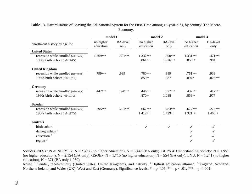
79

Table 13. Hazard Ratios of Leaving the Educational System for the First-Time among 16-year-olds, by country: The Macro-

Economy.



education BA-level

only no higher

education BA-level

only no higher

education BA-level

only

United States

recession while enrolled (ref=none) 1.369*** .501*** 1.332*** .500*** 1.331*** .471*** 1980s birth cohort (ref=1960s) .861*** 1.026*** .858*** .984

United Kingdom

recession while enrolled (ref=none) .799*** .989 .780*** .989 .751*** .938 1980s birth cohort (ref=1970s) .859** .987 .894* .823***

Germany

recession while enrolled (ref=none) .442*** .378*** .446*** .377*** .432*** .417*** 1980s birth cohort (ref=1970s) .870** 1.088 .858** .977

Sweden

recession while enrolled (ref=none) .695*** .291*** .667*** .283*** .677*** .275*** 1980s birth cohort (ref=1970s) 1.412*** 1.429** 1.321*** 1.466**

controls birth cohort

✓ ✓ ✓ ✓

demographics 1 ✓ ✓ education 2 ✓ ✓ region 3 ✓ ✓

Sources. NLSY’79 & NLSY’97: N = 5,437 (no higher education), N = 3,446 (BA only). BHPS & Understanding Society: N = 1,951

(no higher education), N = 2,154 (BA only). GSOEP: N = 1,715 (no higher education), N = 554 (BA only). LNU: N = 1,241 (no higher

education), N = 371 (BA only 1,959).

Notes. 1 Gender, race/ethnicity (United States, United Kingdom), and nativity. 2 Highest education attained. 3 England, Scotland,

Northern Ireland, and Wales (UK), West and East (Germany). Significance levels: * = p <.05, ** = p < .01, *** = p < .001.

80

Reenrollment structures

The opposite transition – that of reenrollment – is examined among the subsample of students

who have entered the labor market by age 25. Figure 6 plots the Nelson-Aalen cumulative hazard

estimates for each country. It should be noted that the x-axis still contains a range from 0 to 120

months, but here it reflects the number of months since the first school-to-work transition (instead

of number of months since age 16, as is the case for the school leaving models). These cumulative

hazard plots indicate a relatively fast reenrollment likelihood for school leavers in Germany and

the United States, followed by Sweden. Educational reenrollment is much less prevalent in the

United Kingdom.

In this section, the emphasis will be on the distribution of reenrollment likelihood for

school leavers who have most to gain from attaining more education: school leavers who first

transitioned to the labor market with no higher education degree. What are the determinants of

educational reenrollment into college after transitioning from school to work before age 25? The

analyses are split by students who never enrolled in higher education before the initial labor market

entry and students who attained some higher education before the initial labor market entry, but

never graduated.

Within each of the four countries, demographics and social background factors are

associated with higher or lower reenrollment chance in the first ten years after labor market entry.

The hazard ratios of the following individual-level variables are documented in Appendix C:

gender, race/ethnicity, immigrant background, region, and age, marital status, and children (of any

age) at the time of entering the labor market. Chapter 4 of this dissertation discusses these factors

in greater detail for the United States, as well as their implications for social inequality.

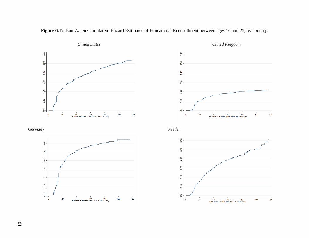
81

Figure 6. Nelson-Aalen Cumulative Hazard Estimates of Educational Reenrollment between ages 16 and 25, by country.


Germany Sweden

82

Of major importance in this chapter is the effect of labor market conditions and rather large

macro-economic signals on educational reentry. The market conditions are measured by the

unemployment rate at initial labor market entry and the state of the economy is measured by a

dummy variable indicating a recession (1) or no recession (0) at initial labor market entry. Table

14 reports the hazard ratios of the market fluctuation (model 1) and the state of the economy (model

2), as well as the hazard ratios of both measures in model 3. All models control for all previously

mentioned individual-level variables.

The results for the United States indicate a significant negative association between a

higher unemployment rate and educational reentry chance (.905 - .909, model 1), as well between

a recession and educational reentry chance (.909 - .790, model 2). This effect was found among

both types of school leavers – those who did not complete high school and those who did not

complete a higher education degree (AA or BA). Moreover, when both the unemployment rate at

entry and the macro-economic condition at entry are put in the same model (3), there are no

substantive changes in the hazard ratios of either predictor on educational reentry. In other words,

when holding constant the variation in the effect of a recession on unemployment rates and vice-

versa, American school leavers become more risk averse toward educational attainment in more

difficult macro-economic times.

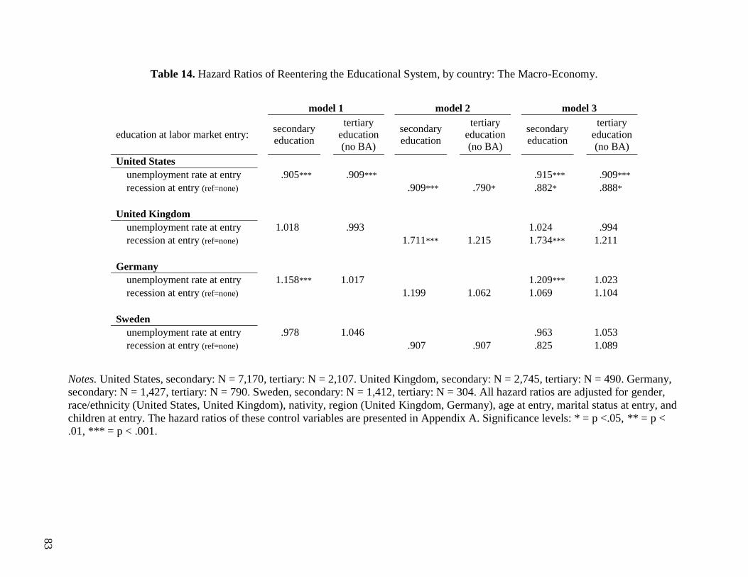
83

Table 14. Hazard Ratios of Reentering the Educational System, by country: The Macro-Economy.


education at labor market entry: secondary

education

tertiary

education

(no BA)

secondary

education

tertiary

education

(no BA)

secondary

education

tertiary

education

(no BA)

United States

unemployment rate at entry .905*** .909*** .915*** .909*** recession at entry (ref=none) .909*** .790* .882* .888*

United Kingdom

unemployment rate at entry 1.018 .993 1.024 .994 recession at entry (ref=none) 1.711*** 1.215 1.734*** 1.211

Germany

unemployment rate at entry 1.158*** 1.017 1.209*** 1.023 recession at entry (ref=none) 1.199 1.062 1.069 1.104

Sweden

unemployment rate at entry .978 1.046 .963 1.053 recession at entry (ref=none) .907 .907 .825 1.089

Notes. United States, secondary: N = 7,170, tertiary: N = 2,107. United Kingdom, secondary: N = 2,745, tertiary: N = 490. Germany,

secondary: N = 1,427, tertiary: N = 790. Sweden, secondary: N = 1,412, tertiary: N = 304. All hazard ratios are adjusted for gender,

race/ethnicity (United States, United Kingdom), nativity, region (United Kingdom, Germany), age at entry, marital status at entry, and

children at entry. The hazard ratios of these control variables are presented in Appendix A. Significance levels: * = p <.05, ** = p <

.01, *** = p < .001.

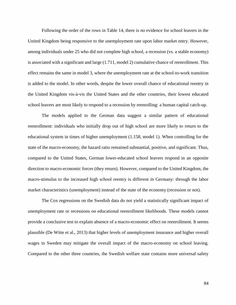
84

Following the order of the rows in Table 14, there is no evidence for school leavers in the

United Kingdom being responsive to the unemployment rate upon labor market entry. However,

among individuals under 25 who did not complete high school, a recession (vs. a stable economy)

is associated with a significant and large (1.711, model 2) cumulative chance of reenrollment. This

effect remains the same in model 3, where the unemployment rate at the school-to-work transition

is added to the model. In other words, despite the lower overall chance of educational reentry in

the United Kingdom vis-à-vis the United States and the other countries, their lowest educated

school leavers are most likely to respond to a recession by reenrolling: a human capital catch-up.

The models applied to the German data suggest a similar pattern of educational

reenrollment: individuals who initially drop out of high school are more likely to return to the

educational system in times of higher unemployment (1.158, model 1). When controlling for the

state of the macro-economy, the hazard ratio remained substantial, positive, and significant. Thus,

compared to the United States, German lower-educated school leavers respond in an opposite

direction to macro-economic forces (they return). However, compared to the United Kingdom, the

macro-stimulus to the increased high school reentry is different in Germany: through the labor

market characteristics (unemployment) instead of the state of the economy (recession or not).

The Cox regressions on the Swedish data do not yield a statistically significant impact of

unemployment rate or recessions on educational reenrollment likelihoods. These models cannot

provide a conclusive test to explain absence of a macro-economic effect on reenrollment. It seems

plausible (De Witte et al., 2013) that higher levels of unemployment insurance and higher overall

wages in Sweden may mitigate the overall impact of the macro-economy on school leaving.

Compared to the other three countries, the Swedish welfare state contains more universal safety

85

nets. The incentive for human capital catchup during economic downturn could be reduced by

these policy structures.

The role of occupational status

Is one’s immediate labor market position associated with higher or lower probabilities of

reenrollment? Table 15 reports the hazard ratios of a categorical variable of the (highest) observed

international socio-economic index (ISEI) of individuals’ job in the first year after the initial

school-to-work transition. This continuous variable was split into tertiles (low, medium, high) and

supplemented with an indicator for no job. All models account for demographics and social

backgrounds and apply all school-leavers with no higher education qualification.

When taking the middle-occupational group as the reference, being employed in the lower

occupational rungs of the labor market makes one less likely to return to the educational system in

three of the four countries: United States (.789), United Kingdom (.609), and Germany (.720).

This contradicts at least one ‘rational choice’ expectation of a higher necessity of human capital

investment for lower occupational positions. Conversely, having a higher socio-economic standing

in the Swedish labor market is associated with increased likelihood of educational reentry (1.296).

How do recessions affect this pattern? Table 16 reports the hazard ratios of an interaction

term between the ISEI category and a dummy for recession at entry. The reference category is

being employed in the middle tertile of the occupational index distribution and experiencing a

recession upon labor market entry. The models for Germany and Sweden indicate no noteworthy

coefficients. The row of interest is the second row of the table, which refers to school leavers who

also experienced a recession when first transitioning from school to work but are in the lowest

occupational group. For both the United States and the United Kingdom, the hazard ratios are

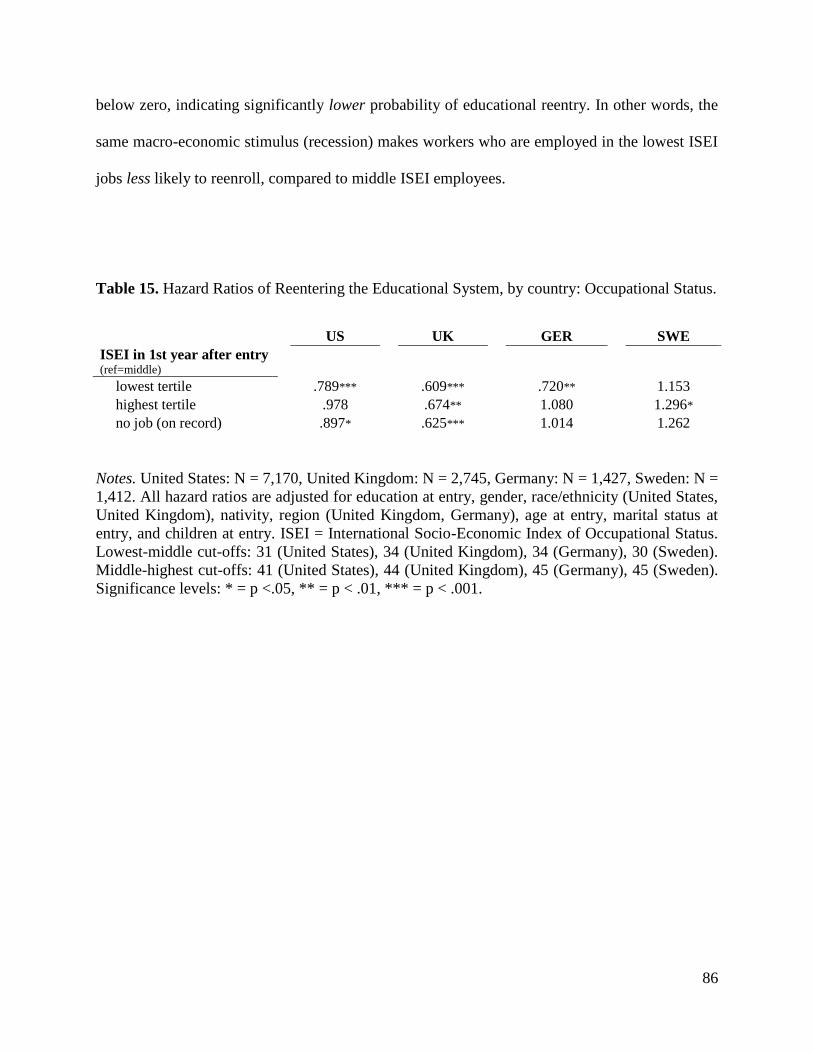
86

below zero, indicating significantly lower probability of educational reentry. In other words, the

same macro-economic stimulus (recession) makes workers who are employed in the lowest ISEI

jobs less likely to reenroll, compared to middle ISEI employees.

Table 15. Hazard Ratios of Reentering the Educational System, by country: Occupational Status.

US UK GER SWE

ISEI in 1st year after entry (ref=middle)

lowest tertile .789*** .609*** .720** 1.153 highest tertile .978 .674** 1.080 1.296* no job (on record) .897* .625*** 1.014 1.262

Notes. United States: N = 7,170, United Kingdom: N = 2,745, Germany: N = 1,427, Sweden: N =

1,412. All hazard ratios are adjusted for education at entry, gender, race/ethnicity (United States,

United Kingdom), nativity, region (United Kingdom, Germany), age at entry, marital status at

entry, and children at entry. ISEI = International Socio-Economic Index of Occupational Status.

Lowest-middle cut-offs: 31 (United States), 34 (United Kingdom), 34 (Germany), 30 (Sweden).

Middle-highest cut-offs: 41 (United States), 44 (United Kingdom), 45 (Germany), 45 (Sweden).

Significance levels: * = p <.05, ** = p < .01, *** = p < .001.

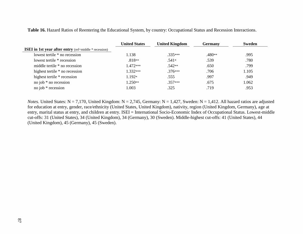
87

Table 16. Hazard Ratios of Reentering the Educational System, by country: Occupational Status and Recession Interactions.


ISEI in 1st year after entry (ref=middle * recession)

lowest tertile * no recession 1.138 .335*** .480** .995 lowest tertile * recession .818** .541* .539 .780 middle tertile * no recession 1.472*** .542** .650 .799 highest tertile * no recession 1.332*** .376*** .706 1.105 highest tertile * recession 1.192* .555 .997 .949 no job * no recession 1.250** .357*** .675 1.062 no job * recession 1.003 .325 .719 .953

Notes. United States: N = 7,170, United Kingdom: N = 2,745, Germany: N = 1,427, Sweden: N = 1,412. All hazard ratios are adjusted

for education at entry, gender, race/ethnicity (United States, United Kingdom), nativity, region (United Kingdom, Germany), age at

entry, marital status at entry, and children at entry. ISEI = International Socio-Economic Index of Occupational Status. Lowest-middle

cut-offs: 31 (United States), 34 (United Kingdom), 34 (Germany), 30 (Sweden). Middle-highest cut-offs: 41 (United States), 44

(United Kingdom), 45 (Germany), 45 (Sweden).

88

Conclusion

Macro-economic shifts and shocks have predictable consequences for school leaving patterns and

reenrollment patterns. On aggregate, higher unemployment and an economy in recessionary state

make young individuals more likely to stay in school longer or to reenter the educational system,

compared to macro-economic stability. The direction of these trends is also well understood from

a Human Capital Theory perspective; both staying in school longer and returning to the educational

system increases one’s competitiveness in a labor surplus market. Recent data capturing the impact

of the Great Recession has also confirmed these patterns.

Using event history analysis applied to data from four post-industrial countries, the hazard

ratio for experiencing a recession while a high school student indicates a higher chance of leaving

the educational system earlier in the United States. Economists call this a ‘discouragement effect,’

causing a student to leave school. This effect held when adjusting for birth cohort (more recent

cohorts stay in school longer), gender, race/ethnicity, and immigrant background. In contrast,

higher education students in the United Kingdom and high school and college students in Germany

and Sweden displayed the expected ‘encouraged student effect.’ They stay in school longer when

the economy is bad. Finally, no school leaving reaction at all to economic downturn (UK college

students).

The unexpected finding for US high school students supports a competing argument to the

rational choice hypothesis for how current students evaluate their post-education chances: the

‘discouraged student effect’ (De Witte et al., 2013). According to these scholars, individuals may

attribute less importance to their own current educational investment as this degree is also

perceived to have less value in the labor market than it did before. However, this explanation is

89

still unsatisfactory and incomplete. Previous studies have only talked about discouragement in

response to the unemployment rate (Tumino & Taylor, 2015), not to the state of the economy

(crisis vs. stable). On the one hand, our models expand the concept of ‘student discouragement’ in

response to the macro-economy; discouragement also occurs when the economy is in a recession.

On the other hand, until studies uncover the link between macro contexts and students’ decision-

making, we cannot know how the process of discouragement operates. Moreover, more research

is needed to understand why US high school students are discouraged by recessions and their

counterparts from comparable economies are not.

Once transitioned from school to the labor force, for the first time, hazard models showed

a significant negative association between entering the labor market during a recession and

educational reenrollment, regardless of being lower- or higher educated members of the labor force

in the United States. In contrast, school leavers in the United Kingdom and Germany become more

likely to reenter the educational system, thereby confirming the human capital catch-up theory.

Furthermore, individuals employed in lower-ranked occupations are also less likely to return to

the educational system in the United States, the United Kingdom, and Germany. Compared to

middle-class workers, a recession makes lower ISEI workers even less likely to return to the

educational system in the Anglo-Saxon countries.

Table 17 presents an overview of the identified influences of the macro economy

(unemployment or recession) and micro conditions (occupational prestige) on both school leaving

and reenrollment. These findings suggest that countries vary in their extent to which risk

perceptions are shaped. Welfare states that are known to have more expensive educational systems

and less protection from social security, like the United States, display more risk averse behavior

among students and young labor market entrants.

90

Table 17. Overview of Identified Macro and Micro Influences on School (re)enrollment, by Country.

Notes. HS = among high school students who never attended higher education. BA = among all college-attending students. <HS =

among students who entered the labor market without a HS diploma. <BA = among students who entered the labor market without a

BA degree (or equivalent.)

staying in education


HS BA HS BA HS BA HS BA

macro predictor

a recession discouraged encouraged encouraged encouraged encouraged encouraged encouraged encouraged

reenrollment


<HS <BA <HS <BA <HS <BA <HS <BA

macro predictor

unemployment rate discouraged discouraged no effect no effect encouraged no effect no effect no effect

a recession discouraged discouraged encouraged no effect no effect no effect no effect no effect

individual predictor

low SEI discouraged discouraged discouraged discouraged discouraged discouraged no effect no effect

91

Chapter 3.

Precarious Early Careers: Instability and Timing within Labor Market

Entry.

Introduction

Employment relations have undergone substantial changes in recent decades. In the United States,

a shift in risk from firms to workers has led to the rise of precarious work. This is an umbrella term

for work that is uncertain, unstable, and insecure, and in which employees bear the risks of work

as opposed to business or government (Kalleberg, 2000; Smith, 1997). These positions are often

(but not always) nonstandard, concentrated in temporary jobs, fixed-term jobs, self-employment,

and part-time jobs. Precarious work is characterized by a profound uncertainty about income and

an enduring risk of unemployment. Moreover, these jobs have relatively lower wages and typically

lack all kinds of benefits, such as medical coverage and pensions, which adds another element to

workers’ vulnerable positions. As millions of US workers are exposed to forms of precarity,

analysts may underestimate existing inequalities in the labor market if they concentrate on

unemployment as the only or major social problem. The rise of precarious work has coincided

with increased job instability since the 1970s. Collectively, these trends form the so-called ‘new

employment narrative’ (Hollister, 2011). This view states that life-long occupations have

disappeared, partially due to government policies that steadily made employment relations more

flexible. Regardless of trends, the relationship between precarious work and job instability is still

92

ambiguous and remains understudied. This partially results from the two-sided definition of

precarious work: it refers to both a static position and highly insecure employment prospects in

the long-term. For instance, one might have a part-time job today, but much of the actual

vulnerability and precarity is experienced in terms unfavorable labor market statuses in the next

month or the next year. Inequalities surface long after the initial exposure to precarious work –

they are situated in the subsequent career patterns and the accumulation of nonstandard work’s

disadvantages.

A gap in the literature exists because nonstandard work is rarely studied in relationship

with the actual precarious career pattern that follows over time. This study concentrates on the

precarity as experienced in its longitudinal form: job instability in work careers. The analyses

present a comprehensive image of a worker’s consecutive vulnerabilities in the labor market. They

concentrate on specific elements and signs of precarious work, such as part-time work, doubling-

up jobs, and the temporality of jobs, in the earliest phase of post-education careers. In doing so,

the start of one’s career – the moment of leaving full-time education for the first time – serves as

𝑡1 after which the next 50 months are modeled in a sequence analysis.

The results indicate both protective and disadvantaging demographic factors and

educational background factors of different types of (precarious) career trajectories. They further

suggest the existence of ‘scarring’ on young individuals’ careers: higher regional unemployment

rates are significantly associated with an increased risk of entering a precarious ‘part-time work’

trajectory and a ‘high unemployment’ trajectory, net of education, industry, and occupation. The

findings contribute to the scholarship of both school-to-work transitions and labor market

inequality.

93

Literature

The new employment narrative

Research on new employment relations has concentrated on a plethora of questions and dependent

variables. In addition to studies about macro shifts within the labor market and the political

economy, three quite uncontested features of individual work careers have been identified.

First, job stability, defined as continuing employment with the same employer, has declined

significantly as the economy has organized around flexible production of services, while relatively

stable employment for lower-skilled workers in manufacturing has largely disappeared. As a

result, unemployment spells and job-switching have become more prevalent features of work

careers (Addison & Surfield, 2009; Mishel, Bernstein, & Shierholz, 2009). This rise of volatility

within US careers is documented through cohort analyses of the National Longitudinal Survey of

Youth 1979 (Bernardt et al., 2001) and the Panel Study of Income Dynamics (Boisjoly, Duncan,

& Smeeding, 1998).

Second, several studies have shown an erosion of job ladders or internal labor markets

since the 1970s, which previously provided workers with chances for future promotions and long-

term employment security within their labor market segment (DiTomaso, 2001; Grimshaw et al.,

2001). As these opportunities have decreased, workers have become more likely to switch jobs

within industries and to cross occupational boundaries compared to previous generations (Valcour

& Tolbert, 2003). This has led some scholars to argue that the lifetime employment model has

been replaced by a ‘patchwork career’ in which employment relationships are only minimally

connected to a profession (Mills & Blossfeld, 2006).

94

Third, a slightly different body of research concentrates on the type of employment in

modern economies. As noted by Kalleberg (2009, 2011), both ‘good jobs’ and ‘bad jobs’ have

existed since the emergence of paid employment relations; some jobs have higher pay or better

benefits than others. However, the share of precarious jobs has increased steadily over the past few

decades. That is, more jobs are characterized by their uncertainty, unpredictability, and riskiness.

This polarization is partially rooted in 1970s legislation that lessened workers’ protection from

dismissal. Furthermore, union decline and deregulation expanded employers’ options to

implement temporary jobs, part-time jobs, and layoffs – a basic component (re-)structuring. As a

consequence of reduced worker protections and the emergence of temporary jobs, an array of

vulnerabilities further concentrate in precarious employment, such as irregular (night) shifts and

limited health insurance coverage (Autor & Houseman, 2010).

In practice, these features of ‘new employment’ overlap. Once employed in a precarious

job, workers immediately feel uncertain about their future career. They simply cannot count on the

employment relationship to be of long-term and are also less confident that a comparable new job

will be available in case of a lay-off. This is illustrated by the steady increase in the aggregate level

of perceived job insecurity in the past four decades (Kalleberg, 2009). Moreover, workers

employed in precarious jobs experience large fluctuations from year to year in earnings (Hacker,

2006) and accumulate earnings penalties (Kalleberg, Reskin, & Hudson, 2000). Thus, work

precarity not only applies to the current work position, but it also destabilizes future employment

paths.

95

Unequal exposure to job instability and job precarity

Scholars have identified sharp differences in terms of career volatility across national labor

markets (Mills, Blossfeld, & Klijzing 2006; Brzinsky-Fay, 2007). Yet how much individual

workers are exposed to job instability and job precarity within a labor market depends on the

interaction between several macro conditions and micro factors.

Although job precarity has increased for virtually every type of worker, some groups are

much more vulnerable for such employment than others (Kalleberg, 2012). This is particularly the

case for lower-educated and lower-skilled workers, who are more likely to have fixed-term

contracts and experience unemployment than previous cohorts (DiPrete, 2005).6 In comparison to

whites, all ethno-racial minority groups are more likely to be exposed to unemployment and

displacement from work (Kalleberg, 2009). Kogan (2007) also found that immigrant groups have

vastly different career trajectories than their non-immigrant counterparts. Although most men of

immigrant descent are employed in lower-skilled segments of the labor market, their precarious

careers cannot be fully explained by educational background or human capital.

Furthermore, both gender and household formation contribute to the risk pattern of unstable

and precarious work careers. Women are far more likely to be affected by the consequences of

nonstandard work and mismatching in the labor market (Pedulla, 2016; Vosko, 2000).

Furthermore, both childbirth and marriage are associated with low-pay part-time work, higher exit

probabilities, and lower re-entry probabilities among women (Tienda & Stier, 1996). Family

6 Some sociologists emphasize the class-driven and education-driven components of employment instability

differently, perceiving job precarity merely as a function of workers’ labor market segment rather than an individual

characteristic (Breen, 1997; Mayer & Carroll, 1987).

96

formation generally increases labor market participation of men due to the implied financial needs

of fatherhood (Fouarge et al., 2010).

Early career setbacks

External conditions also play an important role in explaining exposure to job instability, in

particular at the beginning of one’s career. Research has documented that unfavorable macro-

economic conditions are likely to become ‘trigger events’ that subsequently generate new

stratification mechanisms in the following career phases, including reduced reemployment chances

and earnings penalties (Blossfeld et al., 2009). This process is called ‘scarring.’ An unemployment

scar is explained by a combination of a stigma effect of early unemployment, constraints in job

search opportunities, and human capital depreciation as a result of reemployment in a new firm or

industry (Gangl, 2006).

Empirical research on scarring differs across social science disciplines, but can be divided

into two distinct analytical strategies. First, most life course studies published in sociology and

economics apply an individual-level mechanism. Frequently making use of event history analysis,

this line of research studies the extent to which an individual’s initial unemployment impacts their

future likelihood of employment, future earnings level, and the like. Researchers have found

overwhelming evidence for early unemployment leading to so-called ‘low-pay-no-pay’ cycles and

increased career complexity throughout the career (Manzoni & Mooi-Reci, 2011).

Second, demographic-oriented research takes (birth) cohorts as the unit of analysis and

describe how different generations of workers’ labor market statuses are affected by cohort-wide

exposure to macro-economic or social conditions. The underlying mechanism is supposed to

explain the variation employment difficulties between generations rather than within cohorts or

97

age-groups. For instance, Chauvel (2010) found a scarring effect on the average earnings of several

different 5-year birth cohorts of labor market entrants in France. Those who entered in a time of

economic downturn earned substantially less than their counterparts who entered in a strong

economic climate, with better opportunities to find suitable employment and to negotiate earnings.

Using work-life history data from different countries, both analytical strategies have led to

extensive descriptions of career scars (e.g. Luijkx & Wolbers, 2009; Munoz-Bullon & Malo,

2003). With regard to the United States, the most comprehensive research on scarring has relied

on the NLSY’79. Kletzer and Fairlie (2003) concentrate on the monetary penalty of early career

job loss and found that the third consecutive job loss reduced annual earnings by about 12 percent

for men and women, relative to their expected level in case of stable employment. Mroz and

Savage (2006) reach a similar conclusion with regard to recurring unemployment cycles.

One shortcoming of scarring research is rooted in the somewhat arbitrary definitions of the

dependent and independent variables. Oftentimes, rather simplistic snapshot measures or averaged

measures of career instability and precarity are taken as explanandum, such as the ‘chance of stable

employment at age 30’ or the ‘average time spent in temporary jobs’ (Raffe, 2014). Moreover, in

predicting these outcomes, scholars also frequently turn to static independent variables, such as

the ‘time to first significant job’ or ‘unemployed at age 25’. The work biographies in between,

during which actual forms of instability and precarity can be observed, are left out of this earlier

type of analysis.

Career trajectories

A different scholarly field ignores the macro-economic setting and the timing of labor market

entry, but does carefully analyze the dynamic elements of precarity in career trajectories. A

98

commonly used methodology is to derive ‘ideal types’ (clusters) of career trajectories from

sequence analysis on employment histories. This has led to meaningful cross-national comparisons

in Europe (Brzinsky-Fay, 2007; Anyadike-Danes & McVicar, 2010; Scherer, 2001). Each of these

studies distinguished (and visualized) more vulnerable or high-precarity careers from more the

stable full-time employment patterns throughout the life course.

However, the career paths of those just leaving the education system are markedly different

from later stages of careers. School leavers typically go through a job-searching phase in which

they have little work experience on their resumes. They often string together several temporary

jobs and internships before finding a first (salaried) job. As argued by Brzinsky-Fay (2014), such

early careers should therefore be examined holistically – as a period within the life course – instead

of as one immediate event of switching from ‘in school’ on one day to ‘employment’ on the next

day. In practice, only a handful of studies concentrates on the course of school leavers in the labor

market.

Although relevant from a descriptive point of view, these sequence methods alone present

no explanation or prediction of precarity and instability within early careers, neither by individual

background factors nor by event factors (i.e. unemployment). In some studies, however, predictive

models were used to indicate the relationship between various demographic or socio-economic

variables and post-education career trajectories. These include school leavers in Britain in the

1980s (Anyadike-Danes & McVicar, 2005), in Northern Ireand in the 1990s (McVicar &

Anyadike-Danes, 2002), in Spain in the 2000s (Corrales-Herrero & Rodriguez-Prado, 2012),

where significant effects of parental class (education), geography, skills (school grades), and

gender on forms of early career instability were found.

99

Analytical Approach

The exact moment of labor market entry – the timing – is rarely taken as an explanans for school

leavers’ future pathways in the labor market. Moreover, in the field of career trajectory studies

there are no known studies that investigate the combination of both individual-level factors and

macro-economic conditions to understand sorting and selection into different early career

employment paths (Feldman & Doerpinghaus 1992; Vinkenburg & Weber 2012).

This chapter advances the understanding career instability among young individuals in the

labor market by predicting the type of early career sequence with series of individual-level

variables and contextual (macro-economic) variables. First, young individuals’ trajectories in the

US labor market will be mapped using sequence analysis. An optimal matching algorithm

measures each sequence of monthly labor market ‘states’ on a timeline. These strings of monthly

labor market states within work history data therefore capture detailed movements between ‘full-

time employed’, ‘part-time employed’, ‘inactive’, ‘unemployed’, and ‘in education.’ The

researcher then calculates similarities among the huge possible number of paths and creates

typologies of similar trajectories describing the early career. This sequence analysis highlights

unemployment spells, career volatility, and job precarity in its longitudinal form (Brzinskay-Fay

& Kohler, 2010). Although virtually all young adults entering the labor market experience some

instability, early careers may still vary in their extent to which they contain patterns of work

precarity.

Second, the analyses will turn to the question: “how can early career patterns, with varying

degrees of exposure to job instability, be explained?” This requires a combination of sequence

analysis and hypothesis-testing – a methodological advancement that has remained largely absent

100

from trajectory research (Brzinsky-Fay, 2014). Here, the odds of ideal type membership will be

predicted using variables that have been associated with a higher risk of general career instability

and precarity in previous research, such as gender, educational background, and family formation.

In addition, to measure the potential effect of scarring on early career paths, the regional

unemployment rate will be used as a proxy of the macro-economic climate in the period of the

school-to-work transition. This variable was selected because job searching and labor market

matching largely takes place at the regional level (Greenwood, 2014).

Third, a series of regressions should reveal the consequences of following different early

career trajectories for further stratification in the labor market. Some studies have shown a

(negative) association between early job losses and a shortfall in future earnings (e.g. Kletzer &

Fairlie, 2003), but there are no known studies that have looked at how deviations from a stable

early career trajectory may leave more ‘scars’ on future labor market outcomes. Thus, if some

early careers are much more affected by patterns of precarious work than others, the question arises

to what extent such paths lead to the accumulation of early career earnings penalties.

Data and Methods

Data were drawn from a longitudinal study of a representative sample of high school students for

whom both a school-to-work transition and an early career trajectory was observed. The National

Longitudinal Survey of Youth 1997 (NLSY’97) is a sample of youths between the ages of 12 and

16. The baseline study includes 8,984 individuals who were interviewed on a wide range of topics,

such as education, household situation, and employment. A parent questionnaire was also collected

in the baseline year of 1997. Subsequently, interviews were conducted annually and biannually

since 2011. The NLSY’97 is known for its relatively low attrition rate and detailed monthly

101

education and labor market statuses. In additional, regional and national unemployment figures,

as well as information on national recession periods, were drawn from the Bureau of Labor

Statistics.7

The study sample was reduced to 7,490 cases after dropping individuals who never

conducted a follow-up interview, who were already in the labor market in 1997, whose educational

status could not be traced in the initial interview, and for whom no school-to-work transition was

observed between September 1997 and December 2010. Those who transitioned from full-time

education into military service (189) and into prison (22) were also excluded from the analysis.

As this paper concentrates on first-time school leavers, the start of the early career is

defined as the first non-full-time education activity for at least two full school semesters for

students who have never been previously exposed to the labor market. This definition counts

students who simply take a semester off as remaining enrolled, while those who leave for a

considerable amount of time – one year – as in the labor market. Following the labor market entry,

exclusive labor market positions for 50 consecutive months are measured, with an emphasis on

indicators of precarity: full-time employed, multiple jobs (two or more), part-time employed,

education/training, unemployed, and inactive. It is important to note that someone who is enrolled

in any type of part-time or full-time educational program after the initial school-to-work transition

is considered ‘in education/training,’ regardless of having a side-job.8

7 Data were extracted from the bureau’s Local Area Unemployment Statistics. Retrieved from

http://www.bls.gov/lau/lausad.htm#cct.

8 The monthly labor status is derived from a wider range of statuses that were first created with the NLSY data. The

category “part-time employed” is defined as being employed for less than 32 hours per week. Throughout the first 12

months of the early career, less than 5 percent of the statuses consists of a combination of full-time educational

http://www.bls.gov/lau/lausad.htm#cct

102

Subsequently, the optimal matching algorithm available in the SADI-package for Stata was

used to calculate the distance between each individual’s early career trajectory (Halpin, 2014).

This distance measure is based on the idea that the fewer steps (called costs) necessary to make a

set of two sequences equal, the more similar they are. The so-called indel cost (for insertion-

deletion moves) was set at 1 and the substitution costs were generated empirically through the

transition probabilities of labor market states. Using the Ward algorithm, six clusters of typical

early career trajectories for the American school leavers were constructed. Although there is no

particular reason for why there could not be an infinite number of clusters, for the purpose of

manageability and sociologically interpretability, between five and seven clusters were attempted

(Brzinsky-Fay, 2007).9 Further analyses include multinomial logistic regressions predicting cluster

membership, as well as linear regressions predicting earnings five years after labor market entry.10

enrollment and employment.

9 Substitution costs a derived empirically through transition probabilities (see Chapter 5).

10 In order to conduct these analyses, missing data on individuals’ family income (1,961), parental education (1,189),

occupational status (851), and market earnings (391) were imputed 50 times using the MICE-procedure in Stata.

Missing labor market statuses in the career sequence data are imputed 10 times using MICT (multiple imputation for

categorical time-series) up to 12 internal monotone and non-monotone ones within an individual sequence.

Simulations by Halpin (2012) proved the superiority of this type of imputation compared to leaving a separate state

for ‘missing.’

103

Findings

Descriptive statistics

Table 18 provides descriptive statistics of the independent variables of the models predicting

precarious early careers. We will highlight the most important ones for these analyses.

The average age at which individuals entered the American labor market is 19.23. By this

point, about 10 percent were married or cohabiting, while 7.5 percent had one or more dependent

children. Furthermore, most individuals entered the labor market holding a high school diploma

(42%), while about 13 percent of the sample had dropped out and left the educational system with

no credential. A substantial group of individuals started their professional careers with ‘some

college’ experience (20.3%). Roughly 24 percent held a degree from a higher education institution

when they first entered the labor market – associate’s degrees (3.5%), bachelor’s degrees (18.8%),

and post-graduate degrees (1.6%), respectively. These graduates had gone through the higher

education with no meaningful interruptions.

All individuals in this study entered the labor market for the first time between 1997 and

2010. This period covers both the ‘Early 2000s Recession’ and the ‘Great Recession,’ which

affected a substantial proportion of the NLSY’97 respondents. More than 13 percent made the

transition from school to the labor force during one of these two recessions. Others may also have

entered in otherwise unfavorable macro-economic conditions due to (smaller) local fluctuations in

labor demand. The regional unemployment rate (averaging at 4.8%) is calculated for each

individual’s last month in full-time education – the month in which one was presumably job

searching.

104

Table 18. Descriptive Statistics of the Independent Variables.

mean /

proportion SD

demographic variables

gender

male .512 .006

female .488 .006

race / ethnicity 1

non-black, non-Hispanic .701 .005

black .159 .004

Hispanic .128 .003

other .013 .002

family income (1997) 2 $51,843 $608

father's education (years) 12.87 .039

mother's education (years) 12.90 .030

US born .915 .003

transition variables

age at transition 19.23 .028

marital status at transition

single .894 .004

cohabiting or married .106 .004

children at transition .075 .003

ever incarcerated at transition .009 .001

highest diploma obtained at transition

less than high school .132 .004

high school / GED .421 .006

some college .208 .005

associate's degree .035 .003

bachelor's degree .188 .005

post-graduate degree .016 .002

national recession at transition .134 .004

regional unemployment rate (1-month lag) .048 .001

industry / occupation variables year 1

ever employed as intern .016 .002

industry 3

agriculture .009 .001

manufacturing / production .113 .004

trade / transportation .199 .005

services - entertainment / food .167 .005

services - information / professional .107 .004

finance / economic .048 .003

education / social service .127 .004

other .071 .003

105

no employment .160 .004

ISEI (among employed) 4 41.72 .183

unionized (among employed) .071 .003

Notes. Author’s calculations of a selected subsample of the NLSY ’97 (N = 7,490). Sample-

weights applied. Missing observations were imputed 50 times (MICE). 1 The NLSY’97 oversampled black and Hispanic respondents. ‘White’ practically refers to ‘non-

black / non-Hispanic.’ 2 Drawn from the parent questionnaire. 3 All industry and occupation variables are measured annually and correspond to the labor market

status of the respondent as indicated in the first survey interview after the education-to-labor force

transition. 4 Internationally Comparable Measures of Occupational Status of 1988.

Newcomers primarily found their first job in trade and transportation (19.9%), in the

service industries (combined 27.4%), and education (12.7%). However, some 16 percent of the

respondents were unemployed or inactive throughout the year after their first transition from

school to work.

Table 19 presents three snapshots within the first 50 months after leaving full-time

education. The columns indicate the distribution of the selected labor market states and the mean

ISEI among employed individuals. The far-right column indicates the average distribution of labor

market states across the first 50 months of post-education careers, as well as the mean number of

months spent in each of these states.

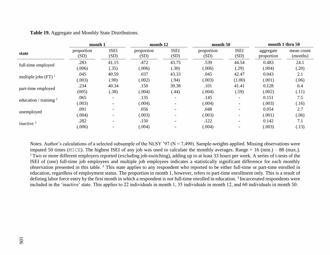
106

Table 19. Aggregate and Monthly State Distributions.

month 1 month 12 month 50 month 1 thru 50

state

proportion

(SD)

ISEI

(SD)

proportion

(SD)

ISEI

(SD)

proportion

(SD)

ISEI

(SD)

aggregate

proportion

mean count

(months)

full-time employed .283 41.15 .472 43.75 .539 44.54 0.483 24.1

(.006) (.35) (.006) (.30) (.006) (.29) (.004) (.20)

multiple jobs (FT) 1 .045 40.59 .037 43.33 .045 42.47 0.043 2.1

(.003) (.90) (.002) (.94) (.003) (1.00) (.001) (.06)

part-time employed .234 40.34 .150 39.38 .101 41.41 0.128 6.4

(005) (.38) (.004) (.44) (.004) (.59) (.002) (.11)

education / training 2 .065 - .135 - .145 - 0.151 7.5

(.003) - (.004) - (.004) - (.003) (.16)

unemployed .091 - .056 - .048 - 0.054 2.7

(.004) - (.003) - (.003) - (.001) (.06)

inactive 3 .282 - .150 - .122 - 0.142 7.1

(.006) - (.004) - (.004) - (.003) (.13)

Notes. Author’s calculations of a selected subsample of the NLSY ’97 (N = 7,490). Sample-weights applied. Missing observations were

imputed 50 times (MICE). The highest ISEI of any job was used to calculate the monthly averages. Range = 16 (min.) – 88 (max.). 1 Two or more different employers reported (excluding job-switching), adding up to at least 33 hours per week. A series of t-tests of the

ISEI of (one) full-time job employees and multiple job employees indicates a statistically significant difference for each monthly

observation presented in this table. 2 This state applies to any respondent who reported to be either full-time or part-time enrolled in

education, regardless of employment status. The proportion in month 1, however, refers to part-time enrollment only. This is a result of

defining labor force entry by the first month in which a respondent is not full-time enrolled in education. 3 Incarcerated respondents were

included in the ‘inactive’ state. This applies to 22 individuals in month 1, 35 individuals in month 12, and 60 individuals in month 50.

107

Many school leavers experienced potentially high-precarity positions during the earliest

stage of the professional career. Across the first 50 months, 12.8 percent of months were spent in

part-time employment, 4.3 percent of months involved holding two jobs at the same time, and

almost 20 percent of months were either unemployed or inactive. The month-level breakdown

further reveals that school leavers are very likely to initially experience a time of non-employment

– a probability of .373 in month 1 and of .206 in month 12 (unemployed and inactive combined).

Things get better over time, but some youths are still at a high risk of being out of the labor market

50 months after leaving the educational system: .048 (unemployed) and .122 (inactive). Moreover,

only 28 percent of school leavers found full-time employment in the first month after the school

career and this number hardly surpasses 50 percent after 50 months (top row).

Nonstandard employment is also closely tied to the occupational level of jobs held. As seen

in each consecutive column of Table 19, the occupational prestige level is the highest in full-time

work positions, as expected. The gap in ISEI between part-time employees and full-time in the

first month after labor market entry is almost indistinguishable (40.3 vs. 41.2, respectively).

However, this gap grows over the course of the early career to a 3-point prestige gap after 50

monthly labor market observations. Although small, this gap is statistically significant.

Similar to part-time jobs, the gap in occupational status between doubling-up jobs and a

single full-time job grows progressively during school leavers’ early careers. As shown in the

second row, the ISEI of workers who juggle multiple jobs at the same time is consistently lower

than full-time employees with a single job in each of the monthly observations (the table only

shows three snapshots). So people tend to combine two bad jobs rather than two good jobs. These

differences are statistically significant for all 50 monthly observations, indicating that a series of

temporary work and doubling-up jobs has some consequences for occupational prestige over time.

108

Early career trajectories

In order to grasp early careers as trajectories as opposed to month-to-month snapshots, each

individual’s sequence of monthly (and exclusive) labor market statuses can be compared to all

other cases in the dataset. The chronograms in Figure 7 present a visual representation of the career

process separately for each of six clusters as found through optimal matching. For each cluster,

the monthly state distribution is plotted vertically and the time line – the first 50 months after the

school-to-work transition – is placed on the horizontal axis. The clusters should be considered

ideal type early careers. Table 20 presents the quantitative characteristics (upper panel) and the

demographic background averages (lower panel) for the six clusters of career trajectories.

One obvious label applies to the cluster that is characterized by a very rapid transition into

full-time work – the bottom-right graph in Figure 7. This ‘full-time career trajectory,’ consisting

of only 16 percent of the school leavers, can be considered the standard employment model in

which both labor market participation and job stability are extremely high. As seen in this graph,

about half the individuals within this cluster enter the labor market in a non-full-time status, but

this drops to less than 10% within 6 months.

A key concept for understanding employment trajectories is the notion of ‘a spell:’ the time

spent in the same labor market position in consecutive months. The larger the number of spells,

the more instability a person experiences. As shown in column 1 of Table 20, the full-time cluster

had an average of 3.7 spells, so even this advantaged group experienced considerable turbulence

in their school-to-work transition. Nonetheless, these are the relative successes among school

leavers and are largely protected against work precarity in terms of job volatility, mismatch, and

underemployment.

109

Figure 7. Chronogram: Early Career Patterns by Cluster.

Notes. Empirical substitution costs, indel cost = 1, optimal matching (OM), cluster Ward.

110

Table 20. Descriptive Statistics of Early Career Labor Force Trajectories.

Cluster

full-time

career

trajectory

precarious I:

part-time

work track

precarious II:

instability

and patching

continued

education work force

to education

unemployed

and

discouraged

sequence characteristics

frequency 1,216 1,213 1,787 1,243 572 1,459

distribution 16.2% 16.2% 23.9% 16.6% 7.6% 19.5%

entropy 1 0.39 1.54 1.29 1.29 1.48 1.36

number of spells 3.7 9.2 8.3 6.3 7.5 9.0

mean spell duration in state

full-time employed 46.3 20.4 31.3 7.8 24.8 8.9

multiple jobs (FT) 0.8 2.1 4.3 0.8 2.1 0.8

part-time employed 0.7 18.0 3.6 5.6 3.3 6.5

education 0.1 1.4 2.9 30.1 15.6 1.3

unemployed 0.8 3.0 3.5 1.5 1.5 6.5

inactive 1.3 5.0 4.4 4.2 2.8 26.1 demographic characteristics

gender

female 36.8% 56.2% 41.2% 56.9% 52.8% 55.5%

race / ethnicity

non-black / non-Hispanic 79.8% 70.6% 72.6% 71.6% 71.0% 53.0%

black 9.4% 15.2% 14.0% 12.7% 15.3% 30.1%

Hispanic 9.6% 12.8% 12.7% 13.7% 12.6% 15.4%

other 1.2% 1.3% 0.6% 2.0% 1.1% 1.5%

family income (1997) $61,455 $47,338 $51,873 $59,956 $56,162 $34,937

father's education (years) 13.17 12.66 12.70 13.69 13.57 11.80

mother's education (years) 13.16 12.77 12.81 13.52 13.60 11.88

US born 92.1% 92.3% 92.7% 87.8% 92.6% 91.8%

111

(continued.)

Notes. Author’s calculations of a selected subsample of the NLSY ’97 (N = 7,490). Sample-

weights are only applied to the averages of the demographic background and earnings variables.

Missing observations were imputed 50 times (MICE). 1 Shannon entropy measure: level of unique

and predictable information within cluster.

In contrast, the cluster labelled as ‘unemployed and discouraged’ captures individuals who

were largely been unsuccessful at finding employment immediately after their labor force entry

and during the following four years (19.5% of the sample). On average, about 26 of the first 50

post-education months in this cluster are spent in ‘inactive’ states (Table 20, column 6). Although

there is a small share of cluster-members with some part-time work (6.5 months) and even full-

time work (8.9 months) during this time period, this cluster mostly reveals a group of young school

leavers who are mainly structurally excluded from the labor market. This strong prevalence of both

employment-seekers and inactivity justifies the tag ‘discouraged.’

In addition to the full-time career trajectory, two other early career types display patterns

with considerable employment participation. However, these have noticeably more components of

employment precarity. First, one cluster consisting of roughly 16 percent of the sample indicates

an extremely high proportion and frequency of part-time employment. This feature is also

relatively consistent across the 50 months after leaving education (Figure 7, bottom-left graph).

As shown in Table 20, respondents selected into this cluster have full-time employment for about

20 out of the 50 months (just below the sample mean). Yet at the same time, they are also far way

more likely to be in a part-time position (18 out of 50 months) – this chance is almost three times

higher than any other career type among the sampled labor market entrants.

This part-time-dominated cluster should not only be defined as ‘precarious’ because of the

disadvantaged nature of part-time work. Their average number of 9.2 spells – the highest among

112

the six identified clusters – also shows that many of these careers are characterized by frequent

transitions in and out of part-time work, full-time work, and unemployment. These young

newcomers most likely seek full-time work but are involuntarily taking temporary employment

when they have to and are consequently involved in a high level of job turnover.

A second type of work precarity comes to the fore in the ‘precarious II: instability and

patching’ cluster. These individuals are slightly more successful in obtaining a full-time job

compared to the sample average, as about 30 out of the 50 months are spent in this status (column

three). However, the combination of high job volatility and high frequency of nonstandard work

hints at a non-trivial disadvantage in this cluster. Similar to the part-time-dominated trajectory,

these careers are highly unstable in terms of transition probability – more than 8 spells on average

in a 50-month sequence. As seen in Figure 7, this type of career starts with a variety of nonstandard

positions (part-time work, double-jobs), as well as education and unemployment. Over the course

of the following four years their educational enrollment declines, but the share of part-time work

remains substantial and that of doubling-up jobs even increases. It suggests an initial phase of

‘patchwork’: unstable employment relationships, in combination with vulnerable work and a high

level of job-switching.

Since first-time labor market entry occurs at a young age (19 to 20 years old) and many do

not hold an educational credential, it is not surprising to observe a ‘early return to education’

pattern (Table 20, column four). Figure 7 also indicates that many of these individuals enter the

labor force and, subsequently, either experience unemployment or are part-time employed after

which many return to the educational system for, on average, 30 out of the 50 months of the early

career. They display the highest level of incomplete college, as 39.2% first enter the labor market

with ‘some college,’ and have a relatively high likelihood (20%) of higher education re-entry

113

within five years (not shown). Although there is no personal-level information available about why

individuals in this cluster re-entered education, it is plausible that they responded to market forces

(e.g. unemployment) or took a planned ‘gap year’ before returning.

Lastly, one distinct cluster of labor market entry is labelled ‘work force to education.’ This

is the least frequently observed type of career trajectory (7.6% of the sample), as seen in column

five of Table 20. The visual progression of this career shows an initial successful entry into full-

time work segment, lasting for about two years, after which substantial numbers return to

education. Again, there is no direct evidence for why individuals return, yet given the time spent

in stable employment it is likely that many return to education to obtain additional degrees –

perhaps in response to market forces.

Demographics and early careers

To what extent do these ideal typical labor market entry paths correspond to different socio-

economic and educational profiles? The lower panel of Table 20 presents the most important

distributions and averages of cluster members’ demographics. Most striking are the sharp gender

differences with regard to accessibility of the full-time career trajectory (63.2% male, 36.8%

female). Conversely, women are overrepresented in the (precarious) part-time work trajectory

(56.2%), yet men make up the highest share in the ‘instability and patching’ trajectory. Moreover,

majority (white) respondents are overrepresented in the full-time career cluster, while black school

leavers make up a disproportionate share of the unemployment-dominated trajectory (30.1%).

Measures of socio-economic class background suggest that school leavers from more

privileged families are concentrated in the stable full-time trajectories; their parents’ average

income of $61,455 is about $10,000 above the sample average. In contrast, the group of labor

114

market entrants exposed to the lowest chance of employment – ‘unemployed and discouraged’ –

come from more disadvantaged family backgrounds. Their family’s income is about $35,000 and

their parents have by far the lowest educational attainment of all clusters (11.8 years).

A multinomial logistic regression predicting one’s early career type is presented in Table

21. This model includes all individual-level demographics (race, gender, family background),

educational background (highest degree at entry), and relevant demographics at the moment of the

school-to-work transition (age, marital status, number of children, incarceration history). The table

presents the estimates of the relative risk ratio (RRR), indicating the relative likelihood of cluster

membership associated with an increase in the predictor, while adjusting for all other predictors.

Given the interest in the factors associated with deviation from the standard career model, the ‘full-

time career trajectory’ is selected as the reference category. Most conservatively, each RRR should

be read as the effect on the odds of experiencing a less successful or less standard early career.11

Women who enter the labor market are significantly more likely to be part of any of the

non-full-time career clusters than their male counterparts. This is remarkable given the gender

equality in terms of educational attendance at the school-to-work transition. Moreover, the model

controls for plausible factors that could influence a deviation from the ideal type full-time path,

such as marital status and number of children. Despite these (non-significant) controls the

disadvantage of women entering the labor market is evident.

11 The estimates of the relative risk ratio were obtained by Stata’s rrr-function which is based on: 𝑒𝑐𝑜𝑒𝑓.. Following

Camey et al. (2014), the threshold at which the odds ratio and the relative risk ratio are interchangeable is a predictor

prevalence level of approximately 10 percent. This conservative rule of thumb is applied in this study.

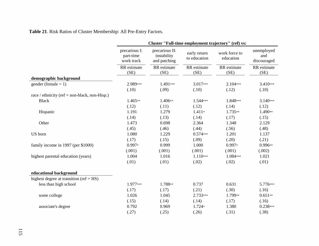
115

Table 21. Risk Ratios of Cluster Membership: All Pre-Entry Factors.

Cluster "Full-time employment trajectory" (ref) vs:

precarious I:

part-time

work track

precarious II:

instability

and patching

early return

to education work force to

education

unemployed

and

discouraged

RR estimate

(SE) RR estimate

(SE) RR estimate

(SE) RR estimate

(SE) RR estimate

(SE)

demographic background

gender (female = 1) 2.989**** 1.491**** 3.017**** 2.104**** 3.410****

(.10) (.09) (.10) (.12) (.10)

race / ethnicity (ref = non-black, non-Hisp.)

Black 1.465**** 1.406**** 1.544**** 1.848**** 3.140****

(.12) (.11) (.12) (.14) (.12)

Hispanic 1.191**** 1.279**** 1.411**** 1.735**** 1.490****

(.14) (.13) (.14) (.17) (.15)

Other 1.473**** 0.698**** 2.364**** 1.348**** 2.129****

(.45) (.46) (.44) (.56) (.48)

US born 1.080**** 1.229**** 0.574**** 1.201**** 1.137****

(.17) (.15) (.09) (.20) (.21)

family income in 1997 (per $1000) 0.997**** 0.999**** 1.000**** 0.997**** 0.996****

(.001) (.001) (.001) (.001) (.002)

highest parental education (years) 1.004**** 1.016**** 1.110**** 1.084**** 1.021****

(.01) (.01) (.02) (.02) (.01)

educational background

highest degree at transition (ref = HS)

less than high school 1.977**** 1.788**** 0.737**** 0.631**** 5.776****

(.17) (.17) (.21) (.30) (.16)

some college 1.026**** 1.045**** 2.733**** 1.799**** 0.651****

(.15) (.14) (.14) (.17) (.16)

associate's degree 0.792**** 0.969**** 1.724**** 1.380**** 0.238****

(.27) (.25) (.26) (.31) (.38)

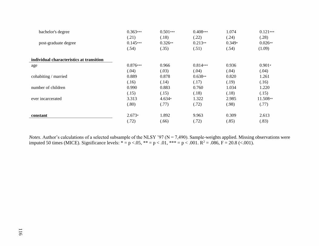
116

bachelor's degree 0.363**** 0.501**** 0.408**** 1.074**** 0.121****

(.21) (.18) (.22) (.24) (.28)

post-graduate degree 0.145**** 0.326**** 0.213**** 0.349**** 0.026****

(.54) (.35) (.51) (.54) (1.09)

individual characteristics at transition

age 0.876**** 0.966**** 0.814**** 0.936**** 0.901****

(.04) (.03) (.04) (.04) (.04)

cohabiting / married 0.889**** 0.878**** 0.638**** 0.820**** 1.261****

(.16) (.14) (.17) (.19) (.16)

number of children 0.990**** 0.883**** 0.760**** 1.034**** 1.220****

(.15) (.15) (.18) (.18) (.15)

ever incarcerated 3.313**** 4.634**** 1.322**** 2.985**** 11.508****

(.80) (.77) (.72) (.98) (.77)

constant 2.673**** 1.892**** 9.963**** 0.309**** 2.613****

(.72) (.66) (.72) (.85) (.83)


imputed 50 times (MICE). Significance levels: * = p <.05, ** = p < .01, *** = p < .001. R2 = .086, F = 20.8 (<.001).

117

A similar pattern of disadvantage can be observed for African-Americans and Hispanics.

The coefficients of both ethno-racial groups indicate consistent higher odds of exclusion from

stable full-time careers. Importantly, the model controls for educational background, which is

expected to capture a considerable part of the relative disadvantages in comparison to the majority

group (white). Yet despite the inclusion of this predictor, the ethno-racial gap is still clear with

regard to the type of labor market route.

The effect of social class as measured by parental income is also predictive of type of career

trajectory. None of the RRR-estimates for the five nonstandard career clusters is larger than one

which means that higher family income is positively associated with the chance of a full-time

career start. Conversely, with the full-time trajectory as the reference category, higher family

income is negatively associated with the chance of selection into the ‘part-time work’ track

(column one), and the ‘work force to education’ track (column four), and the ‘unemployed and

discouraged’ track (column five) after leaving the educational system. In other words, while

controlling for other demographics and education, individuals from lower-class backgrounds are

disproportionally exposed to precarity in the form of part-time work and high job turnover at the

start of their work careers, as well as higher odds of unemployment.

The separate parental education variables were merged into one predictor – highest parental

education in number of years – to prevent multicollinearity. A longer educational career of either

parent is significantly associated with both quickly returning to education (column 3) and returning

a few years later (column 4). This mechanism is likely to be driven by the relative risk aversion

among individuals with higher educated parents (Breen, 1997). It is plausible that, regardless of

external forces that steer such decisions, some young adults return to the educational system to

118

complete a degree or to obtain an advanced degree in order to equal their parents’ education level,

which is perhaps also encouraged by parents.

As seen in the second panel of Table 21, the highest educational credential held by labor

market entrants has a very large impact on their selection into different types of labor market

trajectories. Leaving the educational system with no high school degree almost doubles the odds

of joining a precarious track (1.977 and 1.778), while one is more than five times as likely to follow

the high-unemployment path, with the full-time trajectory as the reference for each of them.

Fortunately, those who enter with some incomplete experience in higher education display a high

chance of re-enrollment through either the ‘early return to education’ or the ‘work force to

education’ route: relative risk ratios of 2.733 and 1.799, respectively (columns 3 and 4).

With regard to other diplomas obtained before entering the labor market, any degree from

a tertiary institution creates substantial protection against all five nonstandard career trajectories.

Holding an associate’s degree prior to the school-to-work transition is associated with a relatively

quick return to the educational system and a lower chance of entering the ‘unemployed and

discouraged’ trajectory during the first phase of one’s career (with a high school degree as the

reference group). Furthermore, both bachelor’s degrees and advanced degrees strongly direct early

careers into stable full-time work. This not only shows the stratifying effect of education on the

likelihood of work versus unemployment, it also indicates that the type of work trajectory is highly

impacted by educational attendance from the early start of careers.

Finally, in addition to background demographics and educational history, a series of

individual characteristics at the school-to-work transition are added to the logit model (bottom

rows of Table 21). As seen there, age at the school-to-work transition is negatively associated with

entering a part-time career path, the early return to education path, and the high-unemployment

119

path. So, older individuals tend to enter a less precarious track, even after controlling for their

educational attainment. Cohabiting or being married reduces the chance of quickly returning to

education. Additionally, entering the labor market with a criminal record increases the relative risk

of experiencing precarious work and entering the ‘unemployed and discouraged’ early career, as

expected.

Macro-economic and economic niche effects

Together, the multinomial logistic model identified the how gender, race, class, age, and

educational background are associated with selection into types of early career patterns. However,

as known from previous research, labor market outcomes may in addition be subject to scarring

that occurs through macro-economic forces during decisive periods of one’s career. Here, the

analysis is focused on the specific macro-economic conditions present at the time of the first

school-to-work transition. In Table 22 the multinomial logistic regression predicting the early

career cluster is expanded with a regional unemployment predictor and several occupation and

industry predictors, while simultaneously controlling for all previously discussed demographic

and educational variables.

The top row indicates the RRR for the regional unemployment rate in percent points in the

last month of full-time enrollment in the educational system. This coefficient indicates that the

more challenging the economic environment at the moment of transition from school to work, the

more likely one is to experience precarity in the form of part-time and short-term work (RRR =

1.182), as well as a quick return to education after an initial struggle in the labor market (RRR =

1.130). Since a dummy variable for a national recession in the month of labor market entry is also

included in the model, these relative risk ratios reflect the influence of the regional labor market

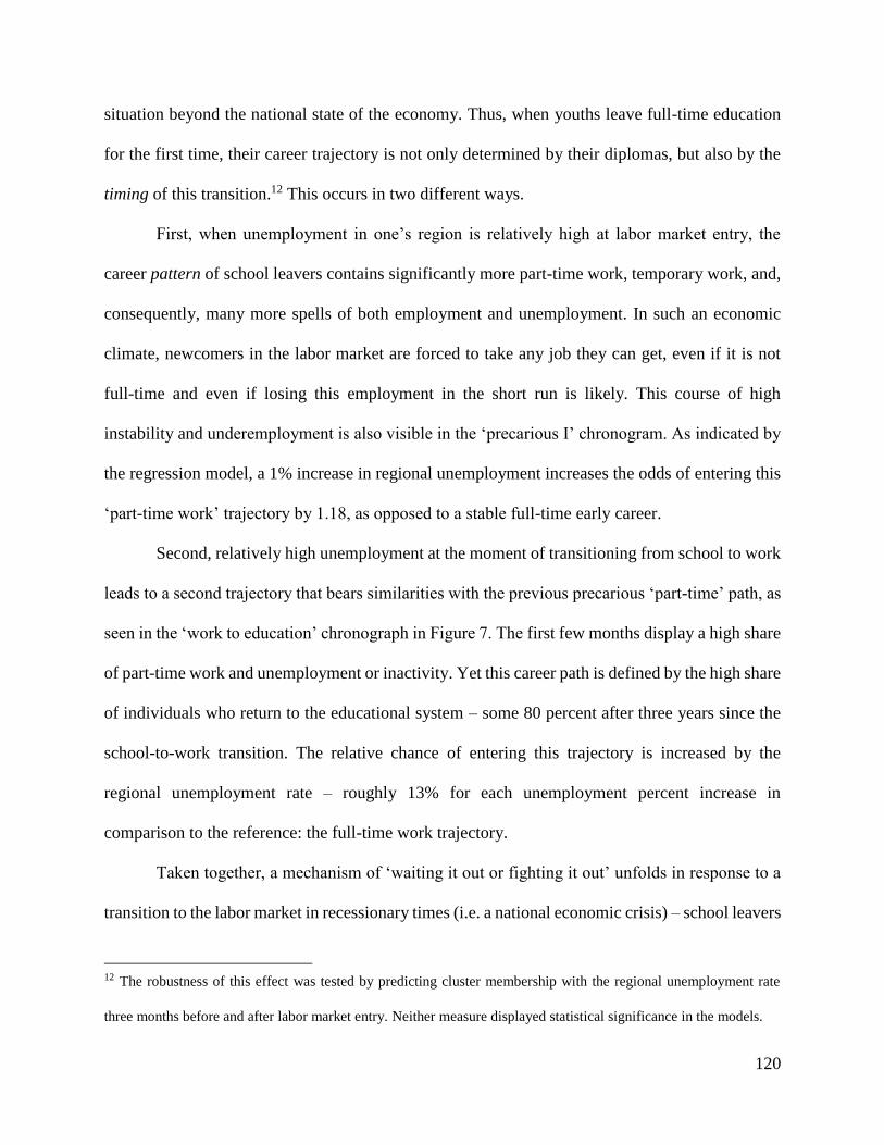
120

situation beyond the national state of the economy. Thus, when youths leave full-time education

for the first time, their career trajectory is not only determined by their diplomas, but also by the

timing of this transition.12 This occurs in two different ways.

First, when unemployment in one’s region is relatively high at labor market entry, the

career pattern of school leavers contains significantly more part-time work, temporary work, and,

consequently, many more spells of both employment and unemployment. In such an economic

climate, newcomers in the labor market are forced to take any job they can get, even if it is not

full-time and even if losing this employment in the short run is likely. This course of high

instability and underemployment is also visible in the ‘precarious I’ chronogram. As indicated by

the regression model, a 1% increase in regional unemployment increases the odds of entering this

‘part-time work’ trajectory by 1.18, as opposed to a stable full-time early career.

Second, relatively high unemployment at the moment of transitioning from school to work

leads to a second trajectory that bears similarities with the previous precarious ‘part-time’ path, as

seen in the ‘work to education’ chronograph in Figure 7. The first few months display a high share

of part-time work and unemployment or inactivity. Yet this career path is defined by the high share

of individuals who return to the educational system – some 80 percent after three years since the

school-to-work transition. The relative chance of entering this trajectory is increased by the

regional unemployment rate – roughly 13% for each unemployment percent increase in

comparison to the reference: the full-time work trajectory.

Taken together, a mechanism of ‘waiting it out or fighting it out’ unfolds in response to a

transition to the labor market in recessionary times (i.e. a national economic crisis) – school leavers

12 The robustness of this effect was tested by predicting cluster membership with the regional unemployment rate

three months before and after labor market entry. Neither measure displayed statistical significance in the models.

121

face two options. While some continue in highly vulnerable career paths after labor market entry,

others quickly return to education to (re-)invest in their skills and credentials. It is plausible that

the latter group is supported directly or indirectly by their families as indexed by parental income

and educational level – their socio-economic position in general – given the significant impact of

these variables for membership of the workforce to education cluster. Alternatively, those entering

the precarious career track clearly lack these family resources (see Table 20).

The fact that macro-economic forces still contribute to the (precarious) character of early

career paths over and above an extensive series of individual-level factors is noteworthy. It

suggests that selection into early career paths is partially affected by the cyclical character of the

economy. School leavers are sorted into career paths primarily as a result of pre-transition

inequalities. The condition of the labor market is however a quite independent external force that

adds to the individual characteristics immediately upon labor market entry. Although some may

be better prepared to mitigate the difficulties of finding stable employment in recessionary times,

macro-economic cycles are not realistically predictable for individuals. The observed effect of

regional unemployment rate on career trajectory merely illustrates the idea that shifts in labor

surplus may affect the early career (in)stability of any young worker; any school leaver; any job

searcher.

122

Table 22. Risk Ratios of Cluster Membership: Macro Conditions, controlling for all pre-entry factors.

Cluster "Full-time employment trajectory" (ref) vs:

precarious I:

part-time

work track

precarious II:

instability

and patching

early return

to education work force to

education

unemployed

and

discouraged

RR estimate

(SE) RR estimate

(SE) RR estimate

(SE) RR estimate

(SE) RR estimate

(SE)

macro-economic context

regional unemployment (1-month lag) 1.182**** 1.102**** 1.130**** 1.056**** 1.074****

(.06) (.06) (.06) (.07) (.06)

national recession (dummy) 1.064**** 0.961**** 1.068**** 1.025**** 0.977****

(.11) (.10) (.11) (.14) (.12)

industry / occupation of entrance year 1

internship 0.369**** 0.890**** 0.878**** 0.805**** 0.342****

(.43) (.33) (.36) (.42) (.56)

unionized job 0.737**** 0.621**** 0.754**** 0.848**** 0.301****

(.17) (.16) (.18) (.20) (.27)

occupational level (ISEI) 0.986**** 0.991**** 0.998**** 1.004**** 0.982****

(.004) (.004) (.004) (.005) (.005)

industry (ref = service-professional)

agriculture 2.079**** 3.443**** 2.973**** 1.800**** 1.084****

(.60) (.54) (.60) (.80) (.71)

manufacturing / production 0.444**** 0.650**** 0.605**** 0.861**** 0.395****

(.20) (.16) (.21) (.23) (.21)

trade / transportation 1.238**** 1.057**** 1.370**** 1.003**** 0.858****

(.17) (.15) (.20) (.21) (.19)

services-entertainment / food 2.114**** 1.790**** 2.785**** 1.723**** 1.494****

(.19) (.18) (.20) (.24) (.21)

finance / economic 0.570**** 0.777**** 0.881**** 0.976**** 0.327****

(.25) (.20) (.24) (.26) (.32)

education / social service 1.505**** 1.525**** 2.350**** 2.254**** 1.018****

123

(.20) (.17) (.20) (.22) (.23)

Other 0.900**** 0.816**** 0.939**** 0.965**** 0.461****

(.20) (.19) (.22) (.26) (.24)

no employment 0.365**** 0.555**** 0.812**** 0.733**** 1.426****

(.20) (.16) (.19) (.23) (.18)

constant 6.253**** 2.180**** 6.713**** 0.282**** 4.579****

(.78) (.72) (.78) (.92) (.88)


imputed 50 times (MICE). Significance levels: * = p <.05, ** = p < .01, *** = p < .001. R2 = .102, F = 13.9 (<.001). Risk ratio estimates

should be interpreted with caution if the prevalence of the predictor is above 10%, in case they should be considered odds ratios. All

industry-occupation predictors refer to the labor market status as indicated by the respondent in the first (annual) survey interview after

the education-to-labor force transition. The ISEI is mean-imputed in case of no employment.

124

The multinomial model predicting the probabilities of various nonstandard early careers

also documents the importance of the economic niche in which one enters the labor market. Based

on the second panel (Table 22) one can conclude that an internship during one’s first year in the

labor force decreases the chance of joining the part-time work track (relative to the reference

category). In addition, being unionized is negatively associated with selection into the precarious

‘instability and patching’ career and the ‘unemployment and discouraged’ career. Hence, these

particular labor market positions shortly after leaving the educational system provide some

protection against the two vulnerable career paths.

The occupation- and industry of first employment after the school-to-work transition is

also highly predictive of the development of the early career. With regard to the former, the

occupational prestige level is negatively associated with the two precarious career tracks, as well

as the high-unemployment path. So, obtaining a higher prestige occupation protects against career

precarity. The largest effects, however, are found among the industry-dummies. These suggest that

starting in the entertainment and food (service) industry increases the odds of the precarious

trajectories, with the risk ratio ranging from 1.790 to 2.114 (Table 22). Similarly, a first job in the

education or social services comes with substantially increased odds of career instability (RRR =

1.5 for both precarious paths) and of returning to education clusters (RRR’s above 2.2). Both these

industries are common among school leavers in the NLSY’97 sample.

Lastly, the last row of Table 22 shows the scarring effect of unemployment at the very start

of one’s career: it increases the chance of a continuation through the unemployment and inactivity

trajectory (column five).

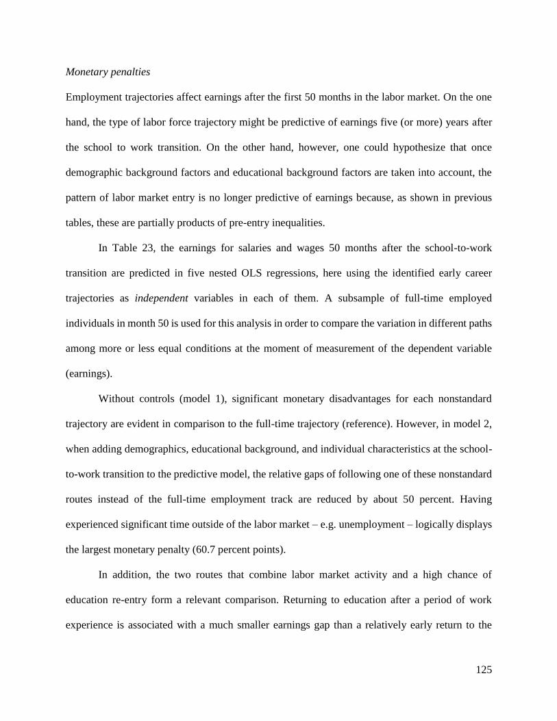
125

Monetary penalties

Employment trajectories affect earnings after the first 50 months in the labor market. On the one

hand, the type of labor force trajectory might be predictive of earnings five (or more) years after

the school to work transition. On the other hand, however, one could hypothesize that once

demographic background factors and educational background factors are taken into account, the

pattern of labor market entry is no longer predictive of earnings because, as shown in previous

tables, these are partially products of pre-entry inequalities.

In Table 23, the earnings for salaries and wages 50 months after the school-to-work

transition are predicted in five nested OLS regressions, here using the identified early career

trajectories as independent variables in each of them. A subsample of full-time employed

individuals in month 50 is used for this analysis in order to compare the variation in different paths

among more or less equal conditions at the moment of measurement of the dependent variable

(earnings).

Without controls (model 1), significant monetary disadvantages for each nonstandard

trajectory are evident in comparison to the full-time trajectory (reference). However, in model 2,

when adding demographics, educational background, and individual characteristics at the school-

to-work transition to the predictive model, the relative gaps of following one of these nonstandard

routes instead of the full-time employment track are reduced by about 50 percent. Having

experienced significant time outside of the labor market – e.g. unemployment – logically displays

the largest monetary penalty (60.7 percent points).

In addition, the two routes that combine labor market activity and a high chance of

education re-entry form a relevant comparison. Returning to education after a period of work

experience is associated with a much smaller earnings gap than a relatively early return to the

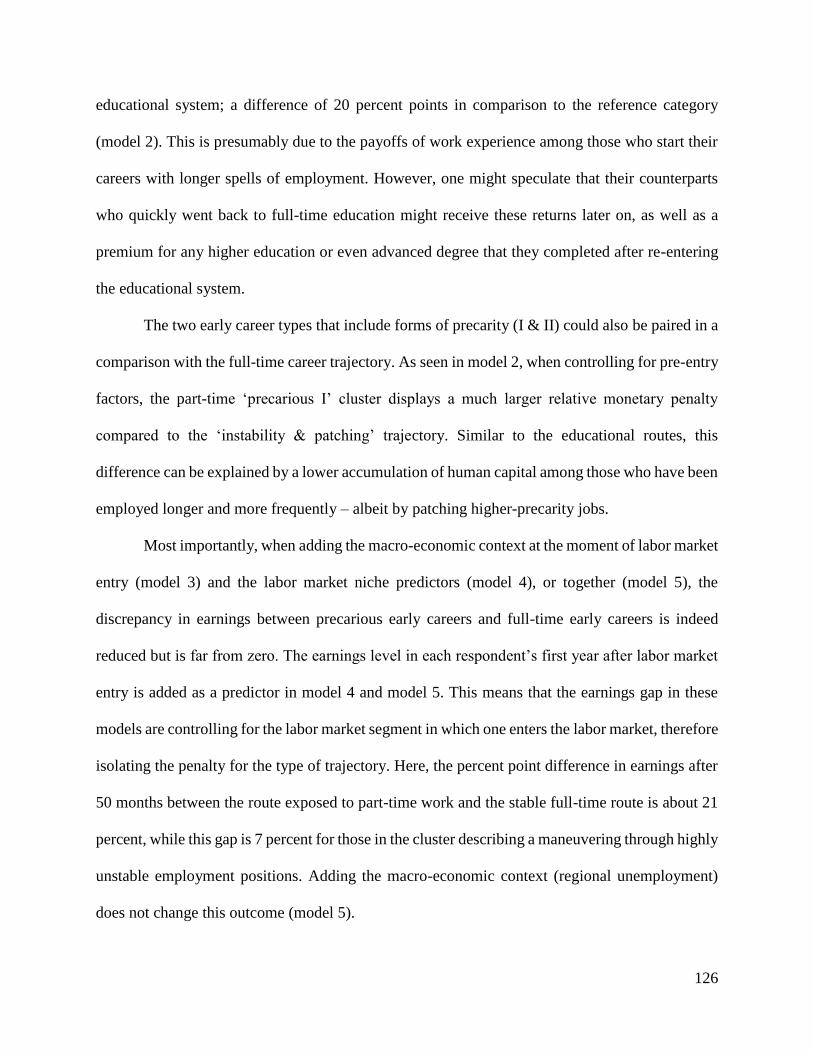
126

educational system; a difference of 20 percent points in comparison to the reference category

(model 2). This is presumably due to the payoffs of work experience among those who start their

careers with longer spells of employment. However, one might speculate that their counterparts

who quickly went back to full-time education might receive these returns later on, as well as a

premium for any higher education or even advanced degree that they completed after re-entering

the educational system.

The two early career types that include forms of precarity (I & II) could also be paired in a

comparison with the full-time career trajectory. As seen in model 2, when controlling for pre-entry

factors, the part-time ‘precarious I’ cluster displays a much larger relative monetary penalty

compared to the ‘instability & patching’ trajectory. Similar to the educational routes, this

difference can be explained by a lower accumulation of human capital among those who have been

employed longer and more frequently – albeit by patching higher-precarity jobs.

Most importantly, when adding the macro-economic context at the moment of labor market

entry (model 3) and the labor market niche predictors (model 4), or together (model 5), the

discrepancy in earnings between precarious early careers and full-time early careers is indeed

reduced but is far from zero. The earnings level in each respondent’s first year after labor market

entry is added as a predictor in model 4 and model 5. This means that the earnings gap in these

models are controlling for the labor market segment in which one enters the labor market, therefore

isolating the penalty for the type of trajectory. Here, the percent point difference in earnings after

50 months between the route exposed to part-time work and the stable full-time route is about 21

percent, while this gap is 7 percent for those in the cluster describing a maneuvering through highly

unstable employment positions. Adding the macro-economic context (regional unemployment)

does not change this outcome (model 5).

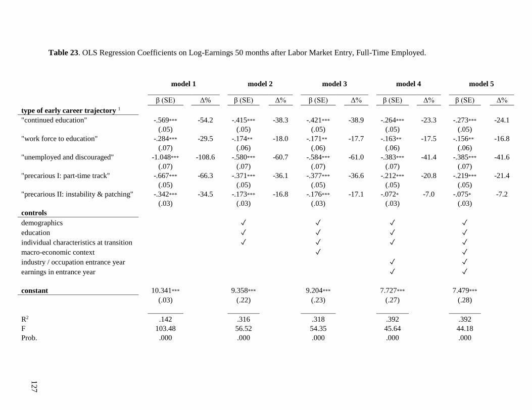
127

Table 23. OLS Regression Coefficients on Log-Earnings 50 months after Labor Market Entry, Full-Time Employed.

model 1 model 2 model 3 model 4 model 5

β (SE) Δ% β (SE) Δ% β (SE) Δ% β (SE) Δ% β (SE) Δ%

type of early career trajectory 1

"continued education" -.569*** -54.2 -.415*** -38.3 -.421*** -38.9 -.264*** -23.3 -.273*** -24.1

(.05) (.05) (.05) (.05) (.05) "work force to education" -.284*** -29.5 -.174*** -18.0 -.171*** -17.7 -.163*** -17.5 -.156*** -16.8

(.07) (.06) (.06) (.06) (.06) "unemployed and discouraged" -1.048*** -108.6 -.580*** -60.7 -.584*** -61.0 -.383*** -41.4 -.385*** -41.6

(.07) (.07) (.07) (.07) (.07) "precarious I: part-time track" -.667*** -66.3 -.371*** -36.1 -.377*** -36.6 -.212*** -20.8 -.219*** -21.4

(.05) (.05) (.05) (.05) (.05) "precarious II: instability & patching" -.342*** -34.5 -.173*** -16.8 -.176*** -17.1 -.072*** -7.0 -.075*** -7.2

(.03) (.03) (.03) (.03) (.03) controls

demographics ✓ ✓ ✓ ✓

education ✓ ✓ ✓ ✓

individual characteristics at transition ✓ ✓ ✓ ✓

macro-economic context ✓ ✓

industry / occupation entrance year ✓ ✓

earnings in entrance year ✓ ✓

constant 10.341*** 9.358*** 9.204*** 7.727*** 7.479***

(.03) (.22) (.23) (.27) (.28)

R2 .142 .316 .318 .392 .392 F 103.48 56.52 54.35 45.64 44.18 Prob. .000 .000 .000 .000 .000

128

(continued.)

Notes. Author’s calculations of a selected subsample of the NLSY ’97 (N = 4,230): full-time

employed individuals 50 months after entering the labor market. Sample-weights applied. Missing

observations were imputed 50 times (MICE). Significance levels: * = p <.05, ** = p < .01, *** =

p < .001. The exact percentage change in outcome associated with one-unit increase of the

predictor is reported in the column next to the regression coefficient (Δ%). The annual earnings

are top-coded at 2% of the reported values (by NLSY’97). 1 Reference = “Full-time employment

trajectory.”

In sum, these models provide evidence that early career patterns affect economic

stratification some four to five years after leaving full-time education for the first time. This effect

is observed in addition to standard predictors of socio-economic status and variables indicating the

labor market industry in which individuals are full-time employed.

Conclusion and Implications

Modern labor markets are increasingly hostile to many workers and in particular to those who were

previously employed in blue-collar production industries. Understanding the inequality-producing

mechanism of exposure to precarious positions in the labor market requires an assessment of its

long-term impact: job instability and continuing cycles of precarious work. There is substantial

knowledge about how bad a job can be and how many ‘bad jobs’ there are in a particular country,

among particular social groups, and cohorts. However, how exposure to these positions unfolds

across career trajectories and how these interact with demographics, life course variables, and

macro-economic conditions has remained understudied. This study measured the risk patterns of

exposure to precarious careers rather than to a single precarious job.

129

By focusing on the early career trajectory (i.e. the first 50 months), this study maps the

passage of school leavers through the various kinds of labor market positions, including those

considered ‘precarious,’ using a representative sample of the American high school population. It

is important to emphasize that these young people in the labor market are markedly different from

mid-career workers because they have limited human capital from work experience. The sequence

analysis approach to the start of careers has not been previously applied in the United States.

The ideal-type careers found using cluster analysis provided several contrasts from the

standard full-time employment trajectory. Two distinct patterns indicate a re-entry into the

educational system, mostly for short periods of time; one involves a rather quick return shortly

after labor market entry, while the second involves a return after several years in the labor market.

Precarity during early careers was also found in two forms: a highly turbulent pattern of alternating

between part-time work, full-time work, and unemployment, as one type, and an unstable

trajectory consisting of stacking multiple jobs and a high risk of unemployment, as the other type.

A third ‘discouraged’ trajectory consists of high unemployment and mostly inactivity.

Among several hypothesized effects of demographic background, the impact of gender

on early career vulnerabilities was surprisingly large. Even after controlling for marital status and

number of children, women are much more likely to experience job precarity through moving in

and out of part-time work and unemployment.

Upon first entering the labor market, both parental social class and race/ethnicity also

displayed strong disadvantages after adjusting for education. To a large extent, these effects

indicate an intergenerational mechanism of stratification with regard to precarity in early careers.

The educational level at labor market entry acted as an additional factor and operated in

the expected direction: job market entrants with a college degree are significantly more likely to

130

experience a stable full-time pathway in the first years in the labor market, while high school

dropouts and high school graduates lack this protection.

Two new approaches to measuring career precarity and instability revealed more

information about the mechanism of scarring and subsequent earnings penalties. Here, scarring

effects of labor market entry were not measured by cohort, as is common in economics and

demography, but instead by the timing of one’s entry into a specific regional labor market. While

controlling for the nationwide state of the economy and the occupation-industry segment, a glutted

regional labor market in the month of entry is associated with a much higher chance both of

entering a highly turbulent trajectory with many part-time work spells and of a quick return to

education. In other words, when school leavers enter a local labor market at an unfavorable

moment, this affects the volatility of their career for several years thereafter. Those who do not

‘fight it out’ in the labor market, may ‘wait it out’ in the educational system, as this seems to be a

plausible alternative for those who can afford to go back to school for a human capital ‘catch-up’

(Mroz & Savage, 2006).

The impacts of demographics, educational level, and the (macro) business cycle are not

limited to just the type of early career experienced in terms of its volatility and intensity. These

various types of trajectories have accumulating effects. After controlling for all background

factors, labor market segment, and earnings level at labor market entry, those school leavers who

experienced a part-time-dominated early career trajectory earn about 20 percent less than stable

full-time employed entrants five years later, even if they hold a full-time job at that point. More

surprising is that the other high precarity pathway – with a high risk of job switching, yet

substantial labor market experience – is also associated with a significant earnings penalty of 7

percent after five years.

131

Concerns have been raised about youths exposed to unemployment at the start of their

careers and whether this produces a ‘lost generation’ (Wolbers, 2014). This paper cannot address

the trend over time with regard to career precarity. However, it does document that different social

groups are channeled into early pathways with different levels of precarity. It indicates how labor

market stratification is affected by some demographics (gender and race) as well as by macro-

economic conditions, which cannot be attributed to the selection and sorting mechanisms of the

educational system. More specifically, timing of entry serves as a trigger event for varying

precarity patterns during the early career.

As noted by Barone and Schizzerotto (2011), scarring from early career unemployment

may affect entire work biographies. Therefore, future research is needed to address how the

revealed scarring effect of the regional labor market conditions impacts unequal labor market

pathways beyond the first five years in the active labor force.

132

Chapter 4.

Macro-Economic Influences on Educational Reenrollment: Human Capital

Catch-Up or Acquired Risk Aversion?

Introduction

A range of well-established sociological theories explain aggregate educational attainment over

time and between cohorts, as well as differences in individual attainment as a complex function of

class, gender, race, ethnicity, and age. Many of these theories were developed under the

assumption of a triphasic industrial life course: first, educational preparation, followed by an

occupational career, and then retirement. In other words, the sociological understanding of labor

market stratification relies heavily on human capital acquisition in terms of years spent in

education or the highest degree obtained prior to the so-called school-to-work transition.

However, over the past 20 years, social scientists have increasingly stressed the

outdatedness of labor market stratification models that assume a simple sequential route from

education to work. In today’s economy the connection between educational preparation and work

life outcomes it is much better understood as a (complex) life course trajectory rather than simple

one-time transition from school to the labor force (Bruckner & Mayer, 2005; Jacob & Weiss,

2010). When many people move from education to work and back to education, while others work

while still in school or college, the concept of labor market entry becomes increasingly problematic

(empirically and theoretically).

133

Students today tend to have longer initial educational careers than in years past and, at the

same time, return to education much more frequently. National Center of Education Statistics

(NCES, 2014) reported that today’s share of adult college students (25 years or older) constitutes

about 42 percent of the total undergraduate student population. Educational sociologists have thus

been increasingly concerned with the various diffuse and scattered relationships between

education, training, and work. In an early literature review, Pallas (1993) states that the recent

differentiation observed in life course transition to adulthood is to a large extent a consequence of

increased heterogeneity in educational careers. Empirical studies initially focused on the phase

between high school graduation and higher education enrollment, especially looking at delayed

entry into college (Goldrick-Rab & Han 2011; Hearn, 1992; Rowan-Kenyon, 2007). Subsequent

research examined ‘stop-out patterns’ in higher education (Desjardins, Ahlburg & McCall, 2006).

Together, this body of literature has led to an important update of our understanding of

educational reentry, including individual-level motivations; opportunities and constraints

associated with returning to education. While previous research generally positioned educational

reenrollment in long-term life course patterns, this paper focuses on the pull factors and push

factors within the early career; the phase immediately after the initial school-to-work transition.

Using data from the National Longitudinal Survey of Youth 1997, the analyses reveal how

the state of the economy upon first leaving the educational system contributes to reenrollment

decisions during the early careers of first-time school leavers. Conditional on a wide range of

demographic factors, survival hazard models provide evidence for two separate mechanisms. First,

consistent with human capital theory, in deciding whether to return to higher education, school

leavers with just a high school degree or with incomplete higher education experience are highly

responsive to rising unemployment in the area in which they first entered the labor force and to

134

individual-level job insecurity. Second, contrary to human capital ‘catch-up theory,’ lower-

educated individuals (less than high school graduates) and highly-educated individuals (bachelor’s

degree or more) are both significantly less likely to reenroll if they left the educational system

during a recession.

Literature

Individual-level background factors

Previous studies gathered evidence that one’s level of education prior entering the labor market

was a strong predictor of reenrollment later on (Astone, Schoen, Ensminger & Rothert, 2000;

Elman & O’Rand, 2004; 2007). Although ceiling effects apply to the highest educated, research

showed a positive linear effect of early educational completion on additional human capital

acquisition. However, human capital theory posits that time spent in education after reenrollment

comes with high opportunity costs because adulthood shifts preferences in favor of both leisure

and generating (necessary) income (Stratton, Toole & Wetzel, 2007). In other words, older

individuals are more likely to attribute a lower marginal value to an additional stint of education

relative to non-educational alternatives.

Parental background has also been strongly associated reenrollment patterns, yet not

always uni-directional. One of the most powerful mechanisms is the so-called ‘Matthew effect,’

as first described by Merton (1968) and later applied to cumulative educational life courses by

Kerkhoff and Glennie (1999). It describes the recurring positive relationship between social origin

and educational upgrading, anywhere in the educational system or in the labor market. In a series

135

of papers, Elman and O’Rand (2004, 2007) reveal enduring effects of social origin on reenrollment

propensity, demonstrating that well into the adult life phase educational participation of high-

socio-economic status (SES) individuals widens class inequality. This is a ‘cumulative educational

advantage’ of higher class background on reenrollment. Educational disadvantage accumulation

can also be understood through a lens of relative risk aversion (RRA) theory (Breen & Goldthorpe,

1997): students aim to at least achieve the same degree level as their parents (which is higher for

high-SES students). Studies have largely confirmed the Matthew effect (Jacob & Weiss, 2011;

Oettinger, 1993; Light, 1995; Elman & O’Rand, 2004, 2007)

Although relative risk aversion is a powerful explanation for social origin effects on

reenrollment, it remains silent on the timing of the risk aversion-mechanism. On the one hand,

high-SES students may initially stay in school longer because of high educational expectations and

plentiful resources, thereby increasing the chance of graduating with a BA (or higher) before

entering the labor market for the first time. This would logically reduce their incentive to ever

reenroll (ceiling effect). On the other hand, the same parental resources could trigger a confident

and strategic stop-out and reenrollment trajectory through post-secondary education and even

graduate school, such as a planned ‘gap year’ or professional internships between educational

levels. The latter, in turn, would lead relative risk aversion to positively predict future educational

reenrollment.

Conditional on having entered the labor market, studies report a positive association

between a minority background and reenrollment likelihood. In NSLY’79 data, Jacob and Weiss

(2011) found that African-Americans are more likely than whites to return to education in their

early careers – a finding that is consistent with studies by Elman and O’Rand (2007), Rich and

Kim (1999), and Astone et al. (2000). These findings have been contested by research that suggests

136

minority students are less likely to return to education (DesJardins et al. 2006; Kimmel &

McNeese, 2006).

A clear gender effect on reenrollment after labor market entry appears in the literature:

while adjusting for other relevant factors, women are overrepresented among returning students

(Scala, 1996) and are significantly more likely to return to the educational system during various

life course phases (Jacob & Weiss, 2011). From a life course perspective, any life phase transition

disproportionally affects reenrollment decisions of women, such as geographical moves, divorce,

changing economic security, entry of children into school, and departure of children from home.

Why this is the case is an unsettled empirical and theoretical question. On the one hand, the

educational careers of some (young) women might be interrupted because of childbearing, after

which they reenroll into the same program. Another rational action argument states that women

benefit more than men from educational investments across the life course (Astone et al. 2000).

On the other hand, research on students who have already reenrolled shows that men face fewer

conflicts in meeting family responsibilities than women, which is mostly the result of unbalanced

family roles (Scala, 1996; Home, 1998). Hence, net of other factors, a higher relative chance of

men to enroll is also expected.

Individual’s status in the labor market

Relying on the rationality assumption, instant economic dislocation, such as job loss, is the most

straightforward market-related force that encourages young individuals to reenroll. This ‘needs-

and-resource’ perspective explains how individuals reentering education are often motivated by a

necessity to update job skills in response to their deteriorating position in the labor market

(Settersten & Lovegreen, 1998). Signs of these ad hoc work- and education-decisions have been

137

found in different forms (Kerckhoff, 1996). Net of other effects, researchers found individuals

responding to unstable careers (Elman & O’Rand, 2007), perceived job insecurity (Elman &

O’Rand, 2002; Smart & Pascarella, 1987), and a recent lay-off (Ghilani, 2008; Knapp & Harms,

2002). In NLSY’79 data, Mroz and Savage (2006) find that if confronted with unemployment at a

young age, individuals are more likely to reenroll in education. This is a so-called ‘human capital

catch-up response’.

However, educational ‘refreshing’ is not limited to individuals who experience

unemployment or instability. Workers are also responding to their relative position in the labor

market. That is, relative to equally educated groups, mismatched workers – whose pay or job duties

are low given their educational attainment – tend to feel dissatisfied and may therefore seek

educational updates to improve their position (DiPrete, 1993). Interview data show this dynamic.

Improving one’s employment position is the most important argument in favor of returning to

college (Deterding, 2015) in a recent survey among 25-34-year-olds. These respondents also

supported a narrative of upward social mobility, which illustrates the tight link between economic

imperatives and the symbolic value of education.

In addition to adverse conditions, ‘good jobs’ can also provide incentives for reenrollment.

This perspective, which is not often applied, suggests that above-average employed workers are

more likely to leave the labor market temporarily for an additional credential – e.g. a BA for AA

graduates or an MBA for BA graduates. It is important to note that the same human capital

rationality – maximizing post-education pay-off – also explains this effect. Moreover, some jobs

at the higher end of the occupational spectrum are also more likely to provide opportunities to

return to school as they tend to have more flexible work hours (Kasworm, 2003).

138

Clark (1960, 1980) proposed the ‘cooling-out hypothesis,’ suggesting that individuals act

rationally by downwardly adjusting their educational goals after first-hand (unsuccessful) college

experience. Scholarly research is unsettled on this hypothesis as some studies find evidence for

lower-educated individuals and college dropouts being less likely to reenroll (Brint & Karabel,

1989; Dougherty, 1994; Pascarella, Edison, Nora, Hagedorn & Terenzini, 1998), while others have

not found any such effect in their data (Alexander, Bozick & Entwisle, 2008). In fact, over time,

higher education dropouts increasingly return to college (Goldrick-Rab, 2006).

Macro-economic climate

In addition to their personal experiences in the labor market, macro-economic factors may also

influence individuals’ decision-making regarding reentering the educational system. This literature

is discussed in much greater detail in Chapter 2.

Researchers have revealed that, on aggregate, high local unemployment is predictive of

reenrolling (Light, 1995). Moreover, higher education enrollments are observed during

recessionary years (Elman & O’Rand, 2004), in particular within the community college system

(Betts & McFarland 1995; Fry, 2009).

It is plausible that a poorly performing labor market – with a low number of vacancies and

high unemployment – is the driving force behind the well-established relationship between a

declining (relative) labor market position and a higher reenrollment propensity, causing the human

capital ‘catch-up’ cycles. However, there is also reason to believe that macro-economic conditions,

and in particular recessions, have an independent effect on reenrollment decision-making (or any

market decision). In theoretical economics, the term ‘countercyclical risk aversion’ (or ‘acquired

risk aversion’) describes the process of individuals responding to market signs in a fearful manner

139

if it indicates an economic bust (Cohn, Engelmann, Fehr & Maréchal, 2015). Individuals are likely

to become risk averse if they primed in a recessionary time; becoming less likely to invest,

purchase, or chance position (i.e. returning to education). However, this question – whether macro-

economic conditions affect educational reenrollment patterns – remains understudied, as well as

the direction in which this effect may occur.

Goals and Hypotheses

This study has three major objectives. First, it tests whether previous findings regarding individual

level effects on reenrollment chances still hold for a recent cohort of labor market entrants. Here,

we expect that highly-educated school leavers and older individuals are least likely to return to the

educational system (hypothesis 1). Since push and pull factors are inherently different for

individuals with lower and higher levels of educational completion, the analyses are conducted

separately by educational subgroup. Within these subgroups, it is expected that measures of high

SES are positively predictive of reenrollment chances (hypothesis 2), and that ethno-racial

minorities are more likely to reenroll (hypothesis 3), and that women are also more likely to

reenroll (hypothesis 4), and that parents or married individuals are less likely to reenroll

(hypothesis 5).

Second, individual labor market positions can be associated with the likelihood of

educational reenrollment, conditional on completed education prior to the school-to-work

transition and the most important demographic factors. However, the scholarly field is not in

agreement over the direction in which these relative market positions may impact reenrollment

140

decisions. On one end of the spectrum, lower relative positions may be predictive of higher

reenrollment (hypothesis 6a). But higher relative positions can also serve as springboards for

further educational attainment (hypothesis 6b). Both effects may occur in the same labor market.

Furthermore, the impact of cumulative unemployment and underemployment (part-time work and

nonstandard work) on the odds of reenrollment will be measured in this section.

Third, in previous research, the association between educational enrollment and the state

of the macro-economy is only understood on the aggregate level. There is circumstantial evidence

of high (youth) unemployment affecting college enrollment. This correlation is best noticeable in

the 2007 – 2009 recession. Youth unemployment rose dramatically and peaked at almost 20

percent, while, within the same time span, the share of individuals enrolled in higher education

increased from 38.8% to 42%.

However, very little is known about the relationship between entering the labor market

during a recession (or high unemployment) and educational reenrollment. The main research

question of this chapter is: Conditional on individual-level demographics, how does the macro-

economic climate upon initial school-to-work transition affect educational reenrollment for

individuals from different educational background groups? Based on existing theory, it remains

unclear how reenrollment decisions of young individuals in the labor market may shift as a result

of unfavorable economic conditions (high unemployment) or an economic shock (recession).

Individuals experiencing such conditions could be more inclined to reenter the educational system

for a ‘human capital catch-up’ (hypothesis 7a) or less inclined because they have become more

risk averse (hypothesis 7b).

141

Data and Methods

These reenrollment hypotheses will be tested with data from the National Longitudinal Study of

Youth 1997 – a sample of youths between the ages of 12 and 16 (born between 1980 and 1984).

The baseline study includes 8,984 individuals who were interviewed on a wide range of topics,

such as education, household situation, and employment. An extensive parent questionnaire was

also collected in the baseline year of 1997. Subsequently, interviews were conducted annually

between 1998 and 2011 and biannually thereafter. The NLSY’97 is known for its relatively low

attrition rate and detailed monthly education and labor market statuses. In additional, regional and

national unemployment figures, as well as information on recession periods were drawn from the

Bureau of Labor Statistics (BLS). This study concentrates on the reenrollment processes among

first-time school leavers, consisting of 7,490 after applying filters. All variables are reported in

Table 24.13

In order to measure the factors associated with reenrollment, a series of event history

(survival) analyses were applied to the early career work biographies of the NLSY respondents. In

these analyses ‘survival’ applies to the length of the very first spell in the labor market after leaving

the educational system. Reenrolling in any educational program after that – part-time or full-time

– is considered the event of interest. Time in the labor market is measured in months and up to 50

13 Similar to Chapter 2, the analyses include individuals who left full-time education for the first time and who have

never been in the labor market (except for working while enrolled in education). Consistent with earlier studies on

reenrollment patterns, this definition counts students as still enrolled who simply take a semester off, while defined

those who leave full-time day-time education for a considerable amount of time – one year without full-time

enrollment – as ‘transitioned into the labor market.’

142

months after initial labor market entry. The reported hazard ratios thus apply to the early career

phase. Missing data within work biographies are due to respondents who drop out of the study

prematurely and do not return in any of the subsequent data collection years. Hence, right-

censoring is adjusted for in the predictive models.

After presenting the cumulative survival estimates of subgroups, consecutive models

estimate the educational reentry hazard ratios for specific demographic factors and for other pre-

transition factors to address hypotheses 1 thru 5. For hypothesis 7, the hazard ratios of two macro-

economic measures – regional unemployment and recession (upon initial entry) – will be added to

these models in order to find the adjusted effects of labor market climate on reenrollment

propensity. Finally, the hazard ratios that represent the individual labor market standings should

provide answers to questions related to push and pull factors that are relative to equally educated

peers; i.e. occupational standing and earnings (hypothesis 6).

The impact of these factors are measured in a Cox (1972) proportional hazard regression

model. Each j-th subject hazard of ‘educational reentry’ – ℎ(𝑡|𝑋𝑗) – is found through

ℎ(𝑡|𝑋𝑗) = ℎ0(𝑡) exp(𝑋𝑗𝛽𝑥) [4.1]

where ℎ0(𝑡) denotes the baseline hazard and 𝛽𝑥 denotes the regression coefficients as estimated

from the data. The tables report the exponentiated individual coefficients that should be interpreted

as the ratio of the hazards for a 1-unit increase or decrease in the corresponding covariate.

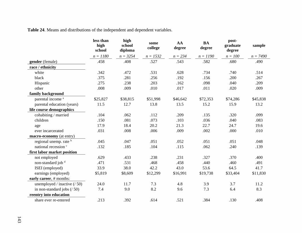
143

Table 24. Means and distributions of the independent and dependent variables.

less than

high

school

high

school

diploma

some

college AA

degree BA

degree

post-

graduate

degree

sample

n = 1180 n = 3254 n = 1532 n = 234 n = 1190 n = 100 n = 7490

gender (female) .458 .408 .527 .543 .582 .680 .490

race / ethnicity

white .342 .472 .531 .628 .734 .740 .514

black .375 .281 .256 .192 .156 .200 .267

Hispanic .275 .238 .203 .162 .098 .040 .209

other .008 .009 .010 .017 .011 .020 .009

family background

parental income a $25,827 $38,815 $51,998 $46,642 $72,353 $74,286 $45,838

parental education (years) 11.5 12.7 13.8 13.5 15.2 15.9 13.2

life course demographics

cohabiting / married .104 .062 .112 .209 .135 .320 .099

children .150 .081 .073 .103 .036 .040 .083

age 17.9 18.4 20.2 21.3 22.7 24.7 19.6

ever incarcerated .031 .008 .006 .009 .002 .000 .010

macro-economy (at entry)

regional unemp. rate b .045 .047 .051 .052 .051 .051 .048

national recession c .132 .185 .104 .115 .062 .240 .139

first labor market position

not employed .629 .433 .238 .231 .327 .370 .400

non-standard job d .471 .531 .468 .458 .440 .460 .491

ISEI (employed) 33.9 38.0 42.2 43.0 53.6 64.5 41.7

earnings (employed) $5,819 $8,609 $12,299 $16,991 $19,738 $33,404 $11,830

early career, # months:

unemployed / inactive (/ 50) 24.0 11.7 7.3 4.8 3.9 3.7 11.2

in non-standard jobs (/ 50) 7.4 9.0 8.2 9.6 7.3 6.4 8.3

reentry into education

share ever re-entered .213 .392 .614 .521 .384 .130 .408

144

Findings

Survival time variation

As shown in Table 24 (that includes all descriptive statistics), the dependent variable – educational

reentry within 50 months after the initial school-to-work transition – is unequally distributed across

the educational background groups. School leavers with an AA degree (50 percent) or ‘some

college’ (60 percent) have higher rates of educational reentry compared to the sample average (40

percent). Returning to education is much less common among both the bottom of the educational

stratum, ‘less than high school’ (21 percent), and the top, post-graduate degree holders (13

percent).

The rate at which school leavers return to the educational system is plotted through a

(cumulative) Kaplan-Meier survival estimate. Figure 8a displays this pattern for the first 50 months

after initial labor market entry for the entire NLSY’97 sample. As shown here, most educational

reentries occur in the first two years of the early career; by month 20, 30 percent of the sample had

returned to the educational system at least once. The smoothed cumulative hazard function (not

shown) also shows the initial increasing chance of educational reentry, followed by a sharply

decreasing chance throughout the rest of the early career.

The survival rates also vary substantially across different levels of educational completion

upon labor market entry (Figure 8b). Both high school graduates and BA graduates display a

survival pattern that is close to the NLSY’97 average. The survival estimates further indicate that

school leavers holding master’s or PhD’s are least likely to return to education, followed by the

similarly shaped survival curve of high school dropouts. College dropouts return are the fastest to

reenter the educational system. Associate’s degree holders have a similar survival rate throughout

145

the first two years in the labor market but are much less likely to reenroll after this period (a

flattening survival estimate). This suggests that reenrollment patterns, and presumably incentives,

are vastly different for educational background groups. Further analyses therefore concentrate on

within-educational level effects.

Separate survival estimates by demographic background factors confirm patterns reported

by the previous literature. As seen in Figure 8c, women return to education at a faster rate than

men do in the first several years after entering the labor market. Furthermore, the higher parents’

educational level, the quicker one returns to the educational system after initial labor market entry

(Figure 8d). This bivariate relationship supports relative risk aversion theory, whereby parental

educational position (e.g. college completion) triggers more educational participation after labor

market entrance.

There is some evidence that the macro-economic state matters for reenrollment odds.

Figure 8e splits the cumulative hazard curve by having left the educational system in a recession

month (stripped line) or a non-recession month (straight line). These seem to indicate that school

leavers who entered during a recession are quicker (and more likely) to reenroll in an educational

program than those who enter when the economy is better. This is in line with the human capital

catch-up response as observed in earlier studies.

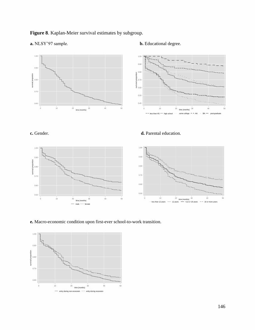
146

0.40

0.50

0.60

0.70

0.80

0.90

1.00

0 10 20 30 40 50time (months)

high schoolless than HS some college AA BA post-graduate

su

riviv

al pro

port

ion

0.50

0.60

0.70

0.80

0.90

1.00

su

rviv

al p

ropo

rtio

n

0 10 20 30 40 50time (months)

less than 12 years 12 years >12 & <16 years 16 or more years

0.60

0.70

0.80

0.90

1.00

0 10 20 30 40 50time (months)

entry during non-recession entry during recession

su

rviv

al p

ropo

rtio

n

Figure 8. Kaplan-Meier survival estimates by subgroup.

a. NLSY’97 sample. b. Educational degree.

c. Gender. d. Parental education.

e. Macro-economic condition upon first-ever school-to-work transition.

0.50

0.60

0.70

0.80

0.90

1.00

0 10 20 30 40 50time (months)

male female

su

rviv

al p

ropo

rtio

n

0.60

0.70

0.80

0.90

1.00

0 10 20 30 40 50time (months)

su

rviv

al p

ropo

rtio

n

147

Demographic and life course factors

Multivariate analyses are necessary to tease out the underlying dynamic of socioeconomic and

educational standing effects on the propensity to reenroll in an educational program after the first

transition into the labor force. Between-group variation is eliminated by estimating the hazard

function separately by educational subgroup. Table 25 presents the Cox regression hazard ratios

of the most important pre-transition predictors of the survival time in the labor market. In each

subsequent column (2 thru 7), the within-educational level effects are reported to evaluate whether

the predictors of interest are representing population-wide mechanisms or rather specific ones.

In a model regressed on all cases, column 1, previously acquired education does not yield

a clear linear and positive relationship to reenrollment probability, as found in earlier studies. With

the high school diploma as the reference category, associate’s degree holders and bachelor’s

degree holders are more likely to reenroll, but this effect is only significant for the former. It should

be noted that these coefficients are adjusted for demographics (as shown), but also the same

relationship was found a bivariate survival regression. Conversely, labor market entrants with post-

graduate degrees are significantly less likely to return to education compared to the reference

group. This ceiling effect among master’s degrees and PhD degrees is understandable as more

human capital investments are unlikely to increase chances in the labor market.

Individuals who drop out of high school are also significantly more likely to remain in the

labor market, regardless of employment status, in comparison to those who had obtained a high

school diploma upon entry (hazard = .506 of returning, column 1). A selection effect is the most

plausible explanation for this finding. Individuals who lose interest in education at a young age or

whose educational aspirations are ‘cooled-off’ early (for varying reasons) are presumably among

the least motivated and least prepared to participate in later schooling.

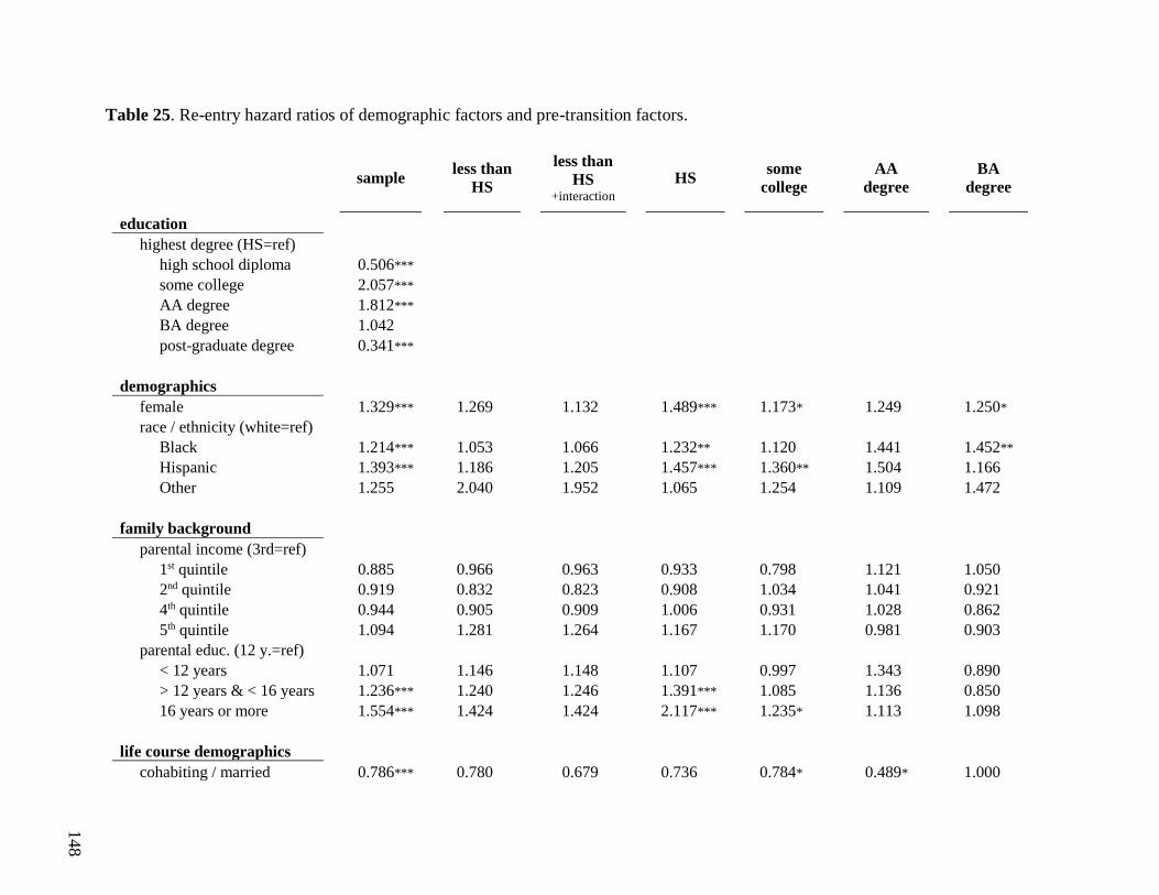
148

Table 25. Re-entry hazard ratios of demographic factors and pre-transition factors.

sample

less than

HS

less than

HS +interaction

HS

some

college

AA

degree

BA

degree

education

highest degree (HS=ref)

high school diploma 0.506***

some college 2.057***

AA degree 1.812***

BA degree 1.042***

post-graduate degree 0.341***

demographics

female 1.329*** 1.269*** 1.132*** 1.489*** 1.173*** 1.249*** 1.250***

race / ethnicity (white=ref)

Black 1.214*** 1.053*** 1.066*** 1.232*** 1.120*** 1.441*** 1.452***

Hispanic 1.393*** 1.186*** 1.205*** 1.457*** 1.360*** 1.504*** 1.166***

Other 1.255*** 2.040*** 1.952*** 1.065*** 1.254*** 1.109*** 1.472***

family background

parental income (3rd=ref)

1st quintile 0.885*** 0.966*** 0.963*** 0.933*** 0.798*** 1.121*** 1.050***

2nd quintile 0.919*** 0.832*** 0.823*** 0.908*** 1.034*** 1.041*** 0.921***

4th quintile 0.944*** 0.905*** 0.909*** 1.006*** 0.931*** 1.028*** 0.862***

5th quintile 1.094*** 1.281*** 1.264*** 1.167*** 1.170*** 0.981*** 0.903***

parental educ. (12 y.=ref)

< 12 years 1.071*** 1.146*** 1.148*** 1.107*** 0.997*** 1.343*** 0.890***

> 12 years & < 16 years 1.236*** 1.240*** 1.246*** 1.391*** 1.085*** 1.136*** 0.850***

16 years or more 1.554*** 1.424*** 1.424*** 2.117*** 1.235*** 1.113*** 1.098***

life course demographics

cohabiting / married 0.786*** 0.780*** 0.679*** 0.736*** 0.784*** 0.489*** 1.000***

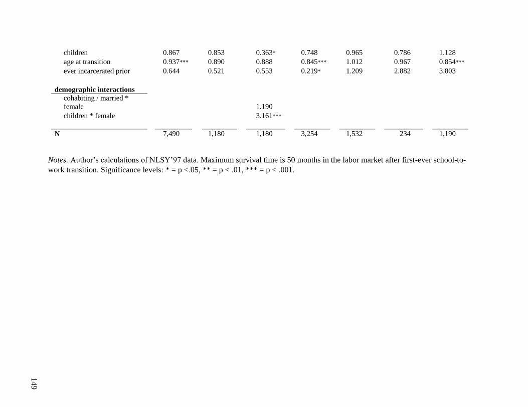
149

children 0.867*** 0.853*** 0.363*** 0.748*** 0.965*** 0.786*** 1.128***

age at transition 0.937*** 0.890*** 0.888*** 0.845*** 1.012*** 0.967*** 0.854***

ever incarcerated prior 0.644*** 0.521*** 0.553*** 0.219*** 1.209*** 2.882*** 3.803***

demographic interactions

cohabiting / married *

female 1.190***

children * female 3.161***

N 7,490*** 1,180*** 1,180*** 3,254*** 1,532*** 234*** 1,190***

Notes. Author’s calculations of NLSY’97 data. Maximum survival time is 50 months in the labor market after first-ever school-to-

work transition. Significance levels: * = p <.05, ** = p < .01, *** = p < .001.

150

If students drop out of college, however, a return to the educational system is highly likely.

As shown in Table 25 (column 1), having some college experience yields by far the highest chance

of reenrollment in comparison to the reference group (hazard = 2.057). Reenrollment is in fact

quite common upon leaving higher education without a degree – 61.4 percent does so within 50

months (Table 24). The incentives to reenroll at this level might be most influenced by the fact

that an important educational milestone is within reach and that this degree may significantly boost

one’s professional career.

The second section of Table 25 presents gender and race/ethnicity effects for the NLSY

sample and the educational sublevels. As expected based on the survival curves and the literature,

women are significantly more likely to return to education than men. However, there is no

significant gender effect among high school dropouts and associate’s degree holders – men and

women are equally likely (or unlikely) to reenroll. Furthermore, confirming the findings in most

previous reenrollment studies, minority students are on average more likely to reenroll compared

to white students. However, when split by highest degree upon initial entry, this effect is only

observed among high school graduates returning to school for higher education after some time in

the labor market. Among higher education attendees, relative to whites, Hispanics are more likely

return to finish the degree after labor market entry.

Social origin is also a strong predictor of labor market entrants returning to education, but

this positive effect is primarily rooted in parental education, and particularly among high school

graduates who entered the labor market (column four). If their parents attained college (12 to 16

years of education) they are more likely to reenroll – and also attend higher education – compared

to high school graduates whose parents never attained college (12 years of education). Moreover,

if their parents completed college or attended graduate school (16 years of education or more), this

151

almost doubles the chance reenrollment among the same group (hazard ratio of 2.117). As seen in

column five, this effect is also positive, and strong, for college goers with incomplete degrees who

have higher educated parents (hazard ratio of 1.235).

In a model with both parental income and parental education, only the latter variable yields

significant hazard ratios. When running a model without parental education (not shown), a high

relative class position (5th parental income quintile) positively predicts reenrollment among high

school graduates and college dropouts / stop-outs (vs. the middle parental quintile group). In other

words, both family background variables show a pattern consistent with the cumulative

ad/disadvantage hypothesis. Since parental educational level trumps income, relative risk aversion

theory is specifically supported.

Life course demographics upon transition

The bottom section of Table 25 presents the hazard ratios of several life-course-specific

demographics that are measured upon first labor market entry (adjusted for demographic and

family background). As seen in column 1, cohabiting or being married (vs. single) is negatively

predictive of educational reenrollment across the entire sample (hazard = .786), but this effect

stems primarily from individuals who attained higher education. Among individuals with some

college experience, being part of a (household) union significantly reduces the likelihood of

returning to the educational system. This effect is even stronger among associate’s degree holders

(hazard = .489).

We also find that women with children are three times more likely (than men with children)

to reenter the educational system, but only if they had dropped out of high school. This suggests a

causal mechanism whereby teenage mothers leave secondary education for some time and then

152

return to high school relatively quickly (within five years). Other interactions – two-way and three-

way combinations of gender, marital status, and children – did not indicate significant effects in

either of the models (therefore not shown).

Confirming earlier findings, the older that school leavers are upon labor market entry, the

less likely they are to (ever) return to education; we find a .937 hazard ratio in the NLSY sample.

However, this age effect seems to occur primarily among high school graduates and post-graduate

degree graduates. Lastly, as expected, having an incarceration record reduces the chance of high

school graduates reenrolling, but this effect should be interpreted with caution as the incidence

rate is extremely low (1%).

Macro-economic effects

The two measures of interest that may capture the impact of the macro-economy upon labor market

entry on educational enrollment patterns are the (regional) unemployment rate (with a 3-month

lag) and a dummy for recession, both by month. In Figure 9, each series of bar graphs indicates

the percent-converted change in odds ratios (from exponentiation of the baseline hazard ratio), as

well as each covariate’s significance for the NLSY sample (a) and each educational level upon

entry (b thru g), separately. To detect potential multicollinearity between the unemployment rate

and the recession variable, the bivariate hazard effects of each predictor on reenrollment are

presented in models 1 and 2, respectively. Model 3 combines both predictors. Model 4 adjusts for

all background demographics and life course demographics (as in Table 25).

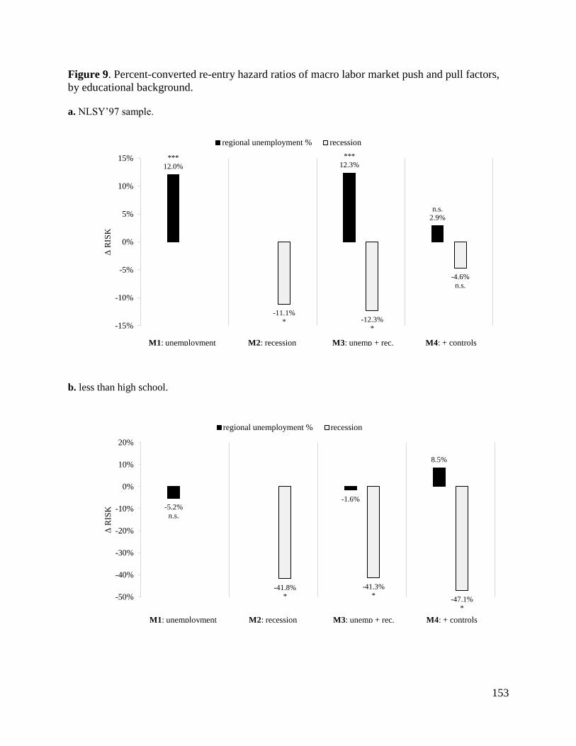
153

Figure 9. Percent-converted re-entry hazard ratios of macro labor market push and pull factors,

by educational background.

a. NLSY’97 sample.

b. less than high school.

***

12.0%

***

12.3%

n.s.

2.9%

-11.1%

* -12.3%

*

-4.6%

n.s.

-15%

-10%

-5%

0%

5%

10%

15%

ΔR

ISK

regional unemployment % recession

M1: unemployment M2: recession M3: unemp + rec. M4: + controls

-5.2%

n.s.

-1.6%

8.5%

-41.8%

*

-41.3%

*-47.1%

*

-50%

-40%

-30%

-20%

-10%

0%

10%

20%

ΔR

ISK



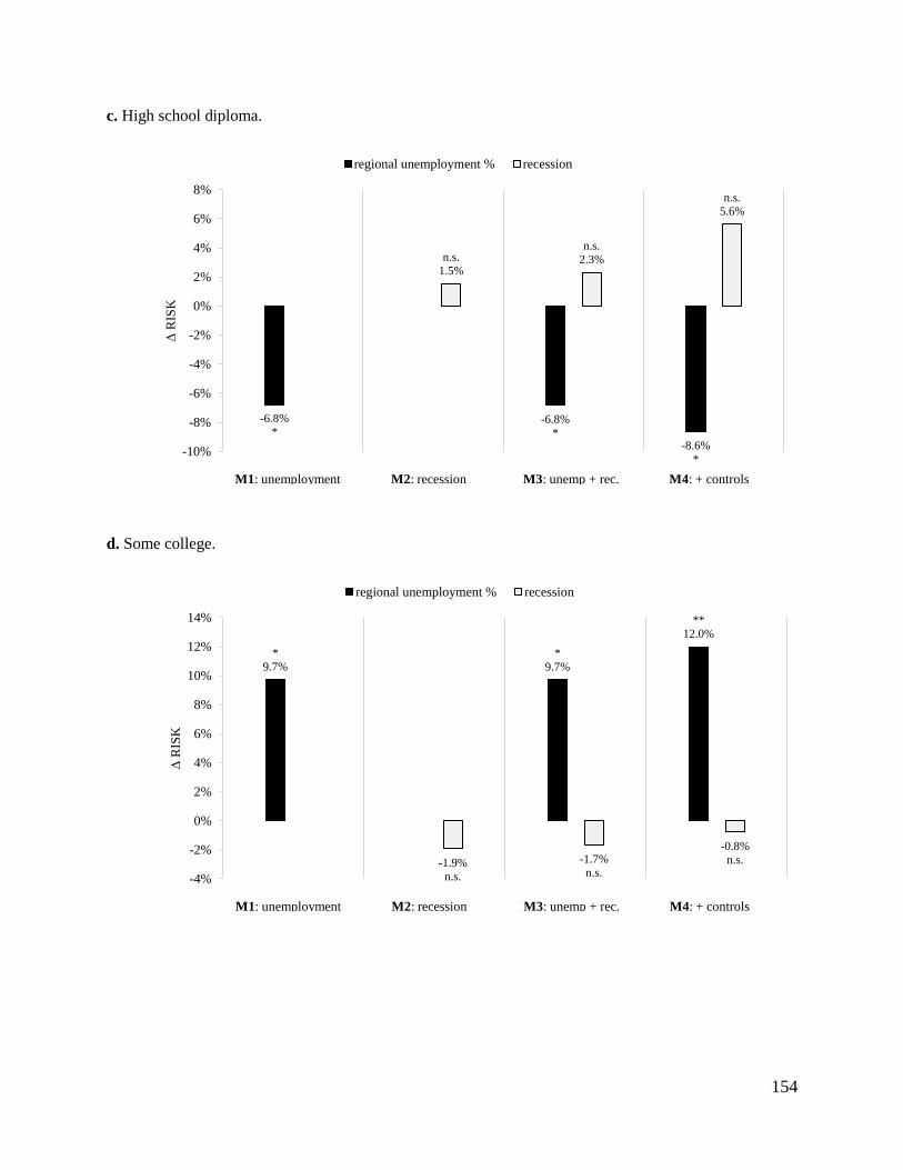
154

c. High school diploma.

d. Some college.

-6.8%

*-6.8%

*-8.6%

*

n.s.

1.5%

n.s.

2.3%

n.s.

5.6%

-10%

-8%

-6%

-4%

-2%

0%

2%

4%

6%

8%

ΔR

ISK



*

9.7%

*

9.7%

**

12.0%

-1.9%

n.s.

-1.7%

n.s.

-0.8%

n.s.

-4%

-2%

0%

2%

4%

6%

8%

10%

12%

14%

ΔR

ISK



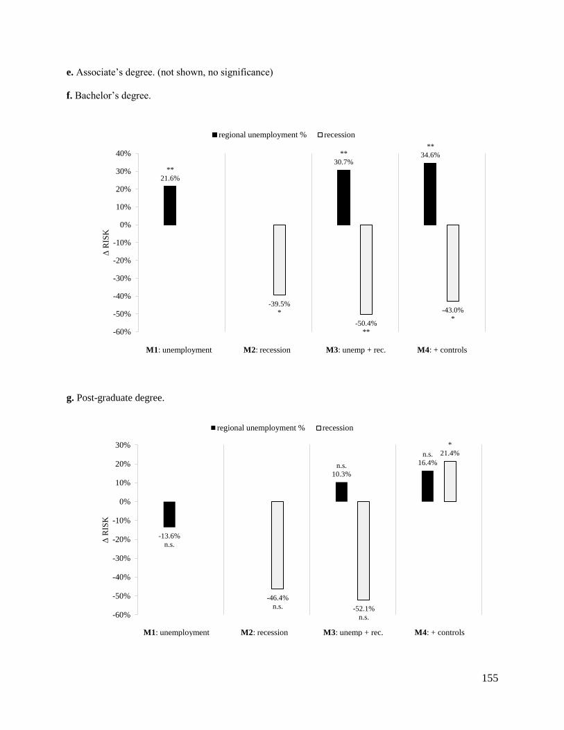
155

e. Associate’s degree. (not shown, no significance)

f. Bachelor’s degree.

g. Post-graduate degree.

**

21.6%

**

30.7%

**

34.6%

-39.5%

*

-50.4%

**

-43.0%

*

-60%

-50%

-40%

-30%

-20%

-10%

0%

10%

20%

30%

40%

ΔR

ISK



-13.6%

n.s.

n.s.

10.3%

n.s.

16.4%

-46.4%

n.s. -52.1%

n.s.

*

21.4%

-60%

-50%

-40%

-30%

-20%

-10%

0%

10%

20%

30%

ΔR

ISK



156

Notes. Author’s calculations of NLSY’97 data. Maximum survival time is 50 months in the labor

market after first-ever school-to-work transition. Model 4 contains all demographic factors

(gender, race/ethnicity, parental income, and parental education) and pre-transition factors

(marital status, number of children, age, and incarceration record). The hazard ratios are

converted into Δ risk – a percent likelihood increase or reduction (conditional on other predictors

in the model. Significance levels: * = p <.05, ** = p < .01, *** = p < .001.

At first impression, paradoxical results appear from a Cox regression on all NLSY

respondents (Figure 9a). As regional unemployment increases (by one percent unit), the odds for

school leavers to reenroll in education within the first four years after labor market entry increase

by about 12 percent (model 1). This suggests a general human capital catch-up response. On

average, young school leavers respond quickly increased labor market competition by gaining

more human capital. However, if the school-to-work transition took place during a recession the

odds of reenrollment are reduced by 12 percent (model 2), even when controlling for the

unemployment rate. As seen in model 4, both effects disappear as the model controls for

demographics and educational background. This indicates that these factors, together, trump the

macro-economic effects or that there is heterogeneity of the macro-economic factors along these

axes.

Combining all educational levels in one model remains problematic to interpret individual-

level or circumstantial effects because incentives for acquisition of additional educational vary

sharply across levels of previous educational attainment. A more sensible approach, therefore, is

to examine measures of the role of the macro-economic climate on early career reentry in separate

models by education (Figures 9b thru 9g). Here, a negative effect of labor market entry during a

recession was found among two subgroups: high school dropouts (Figure 9b, odds reduction of 41

percent) and bachelor’s graduates (Figure 9f, odds reduction of 50 percent). Conditional on all

157

demographic variables and transition variables, school leavers with these educational backgrounds

seem to be held back by a recessionary status of the economy. In other words, for first-time school

leavers with these educational backgrounds, entering the labor market during either in the 2001-

recession or in the Great Recession, reenrollment probabilities shift, negatively, in contrast to their

counterparts who transitioned into a stable labor market.

What is the role of the unemployment rate? The hazard ratios of the regional

unemployment rate present a more varying picture across subgroups. Here, a one percent increase

of unemployment is associated with an 8.6% lower likelihood of educational reenrollment among

high school graduates (Figure 9c, model 4), while controlling for all other predictors. However,

the reverse effect appears among higher education attendees as college dropouts are about 12

percent more likely to return with each one percent unit increase in regional unemployment.

Likewise, bachelor’s degree graduates are also strongly responsive to the regional unemployment.

Their odds of educational reenrollment increase with about 30 percent – presumably to attempt a

post-graduate degree – for each percent-increase in unemployment at the initial school-to-work

transition.

The heterogeneous effects of macro-economic conditions upon labor market entry vary in

both direction and strength among different educational groups, except for associate’s degree

holders among which neither of these two market forces is associated with reenrollment hazards.

Interestingly, both the positive impact of (higher) regional unemployment on reenrollment

probability and the negative impact of entering the labor market during a recession are found

together among bachelor’s degree holders, regardless of other predictors in the model. Thus, a

recessionary economy is yields a substantially different reenrollment mechanism than the main

sign of a poorly performing economy: a labor market with high unemployment.

158

Individual labor market status

How do school leavers respond to individual labor market experiences? Can human capital catch-

up effects be found? Table 26 presents the hazard ratios for several measures of one’s labor market

status, adjusted for all previously reported demographic and transition variables. Each of the

individual labor market predictors are added separately to the models by educational subgroup.

The first labor market status after the initial school-to-work transition is only partially

informative of educational reenrollment (upper Table 26). In comparison to the reference group

(full-time job), part-time employment is positively associated with reenrollment, but only among

those entering as a high school dropout (hazard = 1.913), a high school graduate (1.180), or a

college dropout (1.266). In addition, not having employment at all and not looking for a job (i.e.

‘inactive’) upon labor market entry is an expected predictor of returning to secondary education

(1.774). These findings suggest that an unfavorable position at the very start of one’s labor market

career – but not unemployment – triggers reentering the educational system within 50 months. So

once one stops looking for a job, returning to the educational system becomes more likely.

However, educational reenrollment decisions are likely to develop over the course of the

early career, beyond the initial labor market position. As seen in the second variable row in Table

26, the cumulative number of months out of work (unemployed or inactive) is negatively predictive

of reenrollment among the lower educational subgroups: less than high school (hazard = .938),

high school diploma (hazard = .951), and some college experience (hazard = .957). However,

presented in the third variable row, an accumulation of non-standard employment situations (i.e.

working double jobs and part-time work) in the early labor market career of high school graduates

and college dropouts positively affects the reenrollment propensity. Both groups display a

significant hazard ratio of 1.022.

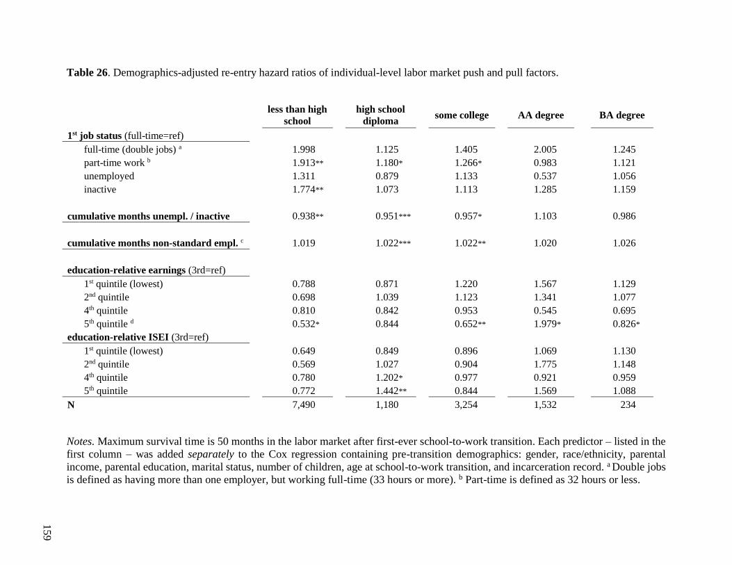
159

Table 26. Demographics-adjusted re-entry hazard ratios of individual-level labor market push and pull factors.

less than high

school

high school

diploma some college

AA degree

BA degree

1st job status (full-time=ref)

full-time (double jobs) a 1.998*** 1.125*** 1.405*** 2.005*** 1.245***

part-time work b 1.913*** 1.180*** 1.266*** 0.983*** 1.121***

unemployed 1.311*** 0.879*** 1.133*** 0.537*** 1.056***

inactive 1.774*** 1.073*** 1.113*** 1.285*** 1.159***

cumulative months unempl. / inactive 0.938*** 0.951*** 0.957*** 1.103*** 0.986***

cumulative months non-standard empl. c 1.019*** 1.022*** 1.022*** 1.020*** 1.026***

education-relative earnings (3rd=ref)

1st quintile (lowest) 0.788*** 0.871*** 1.220*** 1.567*** 1.129***

2nd quintile 0.698*** 1.039*** 1.123*** 1.341*** 1.077***

4th quintile 0.810*** 0.842*** 0.953*** 0.545*** 0.695***

5th quintile d 0.532*** 0.844*** 0.652*** 1.979*** 0.826***

education-relative ISEI (3rd=ref)

1st quintile (lowest) 0.649*** 0.849*** 0.896*** 1.069*** 1.130***

2nd quintile 0.569*** 1.027*** 0.904*** 1.775*** 1.148***

4th quintile 0.780*** 1.202*** 0.977*** 0.921*** 0.959***

5th quintile 0.772*** 1.442*** 0.844*** 1.569*** 1.088***

N 7,490*** 1,180*** 3,254*** 1,532*** 234***

Notes. Maximum survival time is 50 months in the labor market after first-ever school-to-work transition. Each predictor – listed in the

first column – was added separately to the Cox regression containing pre-transition demographics: gender, race/ethnicity, parental

income, parental education, marital status, number of children, age at school-to-work transition, and incarceration record. a Double jobs

is defined as having more than one employer, but working full-time (33 hours or more). b Part-time is defined as 32 hours or less.

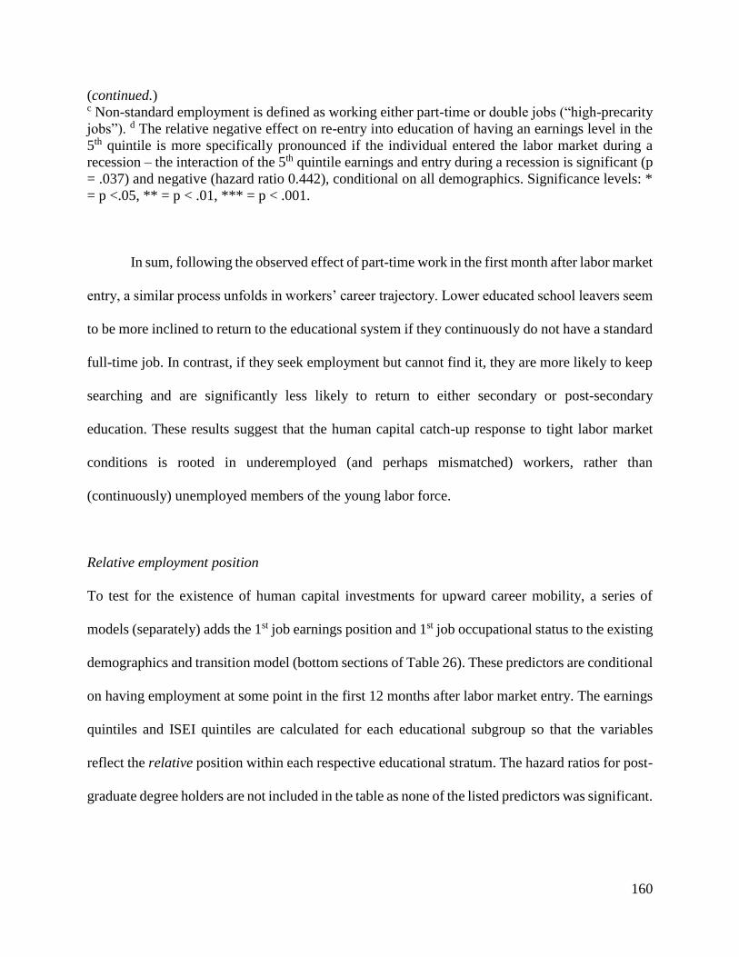
160

(continued.) c Non-standard employment is defined as working either part-time or double jobs (“high-precarity

jobs”). d The relative negative effect on re-entry into education of having an earnings level in the

5th quintile is more specifically pronounced if the individual entered the labor market during a

recession – the interaction of the 5th quintile earnings and entry during a recession is significant (p

= .037) and negative (hazard ratio 0.442), conditional on all demographics. Significance levels: *

= p <.05, ** = p < .01, *** = p < .001.

In sum, following the observed effect of part-time work in the first month after labor market

entry, a similar process unfolds in workers’ career trajectory. Lower educated school leavers seem

to be more inclined to return to the educational system if they continuously do not have a standard

full-time job. In contrast, if they seek employment but cannot find it, they are more likely to keep

searching and are significantly less likely to return to either secondary or post-secondary

education. These results suggest that the human capital catch-up response to tight labor market

conditions is rooted in underemployed (and perhaps mismatched) workers, rather than

(continuously) unemployed members of the young labor force.

Relative employment position

To test for the existence of human capital investments for upward career mobility, a series of

models (separately) adds the 1st job earnings position and 1st job occupational status to the existing

demographics and transition model (bottom sections of Table 26). These predictors are conditional

on having employment at some point in the first 12 months after labor market entry. The earnings

quintiles and ISEI quintiles are calculated for each educational subgroup so that the variables

reflect the relative position within each respective educational stratum. The hazard ratios for post-

graduate degree holders are not included in the table as none of the listed predictors was significant.

161

In order of educational background, for school leavers without a high school diploma,

having a high-paying job relative to the average job-holding high school dropout (3rd quintile) is

negatively associated with reenrollment (hazard = .532). So, given the low employment chance

within this group in general, if one has a good job (against the odds) this pushes an individual

further away from returning to high school to complete a diploma. For high school graduates who

do not immediately enroll in higher education, a strong incentive for upward occupational mobility

is apparent from the significant hazard ratios of employed individuals in the high earning 4th and

the 5th ISEI quintiles (relative to the 3rd quintile), with hazard ratios of 1.202 and 1.442,

respectively.

Once having started in higher education, but not completing any degree, the impact of a

high relative position (in terms of earnings) reverses again; having a job with earnings that fall in

the high earning 5th quintile significantly reduces the chance for a ‘some college’ individual to

reenroll in college. This suggests that some college dropouts who have found good jobs – which

potentially is the reason for dropping out – have satisfied their human capital acquisition. A degree

might seem unnecessary for them for further job chance improvement, at least in the early phase

of their labor market careers.

In contrast, those who complete an associate’s degree and have high-paying jobs (5th

quintile) do display a strong incentive to return to education. They have almost twice the odds

(hazard ratio of 1.979) compared to the average AA graduate to reenroll and attempt a BA degree.

However, if first-time school leavers enter the labor market with a bachelor’s degree, having a

high-paying job negatively predicts reenrollment. Like high-earning college dropouts, most BA

graduates’ skills and education seem satisfactory for obtaining a stable position in the labor market

(so graduate school becomes less attractive).

162

In sum, evidence for upward career mobility incentives was found alongside human capital

satisfaction effects. Both vary sharply depending on the highest educational level with which

school leavers enter the labor market. However, the data do not show evidence for the opposite

effect: a human capital ‘update’ (reenrollment) in response to an unfavorable employment situation

in terms of relative (lower) earnings or occupational prestige.

Discussion

Earlier research about educational reenrollment made use of longitudinal samples drawn in the

1970s (NLSY’79) and the 1980s (early waves of the National Survey of Families and Households).

This study relies on a more recent representative sample of the US high school population in 1997,

who transitioned from school-to-work in the late 1990s and throughout the 2000s.

When comparing the findings of these cohorts, we found similar effects of demographic

background and life course demographics on educational reenrollment propensity. The negative

impact of age and marriage (cohabiting) on reentry are robust, as well as the higher relative

likelihood for women, ethno-racial minorities, and members of higher SES groups to reenroll in

education. The latter effect implies that relative risk aversion continues to occur post initial labor

market entry, as higher parental education is the strongest predictor educational reentry. A person’s

educational level upon labor market entry is linearly (and negatively) related to reenrollment

propensity. Rates of reenrollment are higher for college dropouts than for AA graduates, and

higher for AA graduates than for BA graduates.

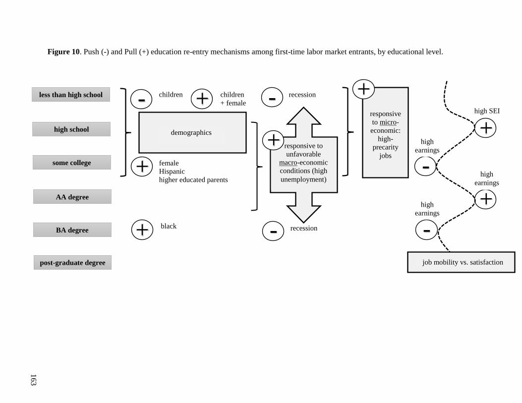
163

recession

high

earnings

high

earnings

high

earnings

+

Figure 10. Push (-) and Pull (+) education re-entry mechanisms among first-time labor market entrants, by educational level.

less than high school

high school

some college

AA degree

BA degree

post-graduate degree

demographics

female

Hispanic

higher educated parents

children children

+ female

black

responsive to

unfavorable

macro-economic

conditions (high

unemployment)

recession

responsive

to micro-

economic:

high-

precarity

jobs

job mobility vs. satisfaction

high SEI

+

+ +

+

+

+

-

- -

- -

164

In contrast to previous studies that concentrated on a single educational level, often times

high school graduates or college graduates, this research reports reenrollment hazards for a wide

range of educational backgrounds. Sample sizes allowed for separate analyses by subgroup and

these lead to more nuanced findings. As shown in Figure 10, demographics, such as gender, race,

and class, play a significant role among school leavers from the lower educational strata. Over and

above these factors, having children is negatively associated with low reenrollment chances

overall, but with higher reenrollment chances for young women.

Of major concern in for study is the question whether, controlling for these well-established

individual-level factors, the state of the macro-economy upon labor market entry triggers

reenrollment patterns. Confirming some parts of human capital theory, and in particular the ‘catch-

up’ thesis, those school leavers who already have some higher education are on average more

likely to update or ‘refresh’ their education in response to a labor market surplus, a high

unemployment rate. Moreover, these effects are quite large; an increase in reenrollment odds of

12 percent (among college dropouts) and 34 percent (among BA graduates) for each percent

increase in the regional unemployment rate, adjusted for background factors. High school

graduates, however, become less likely to reenter (higher) education as the unemployment rate

increases. Relying on these data, more human capital acquisition in times when it is difficult to

find employment seems to be a realistic option only for early career individuals who already started

college.

Unlike earlier research about the contribution of macro-economic factors to reenrollment

decisions, this study looked at whether entering the labor market during a recession leads to a

higher or lower likelihood of returning to the educational system during the early career. The most

important finding is that it does, but not in the direction predicted by human capital theory. Across

165

all educational levels, and as seen Figure 9a, first-time school leavers are less likely to obtain more

education if they are part of a cohort that entered a recessionary labor market. This effect is

independent of a fluctuating unemployment rate, but does not trump demographic factors and the

role of previously obtained education across the entire population. However, for two specific

groups at the very lower educated (less than high school) and the higher educated (BA+ level),

being part of a recession keeps them away from a second stint in education (as illustrated in Figure

10). In other words, these individuals become more risk averse as a result of being part of a cohort

of school leavers that transitioned during a recession. Rather than exploring educational refreshing,

which is common if unemployment is high in one’s region, transitioning into the labor market

during a recession triggers caution: I’d rather hold on to what I have, than take more risks.

How do human capital catch-up decisions operate at the micro level? Primarily at the lower

end of the educational spectrum (Figure 10), individuals in their early career phase who cannot

find stable employment – who are continuously underemployed (part-time work) or in highly

precarious jobs (two jobs) – display the highest likelihood of returning to the educational system,

adjusted for demographics. In contrast, continuously being out of work is associated with a high

propensity to stay (searching) in the labor market. This means that human capital catch-up in

response to a tighter labor market primarily occurs among young individuals who are dissatisfied

with their precarious employment, and not among the unemployed.

In addition, certain demographic pull factors are observed among high school graduates

(enrolling in higher education) and associate’s degree graduates (for enrolling in a BA program).

They are above-average employed (SEI or earnings) and seek ways for further upward job

mobility. These findings confirm a momentum thesis; earlier educational success (i.e. degree

completion) stimulates further educational participation. Conversely, dropping out of college, yet

166

still earning more than one’s counterparts, reduces reenrollment chances, which might be a sign of

job satisfaction.

Future studies should further examine the risk management that influences reenrollment

decisions. For instance, student debt in younger generations of college attendees might well play

an important role when evaluating the opportunity costs of educational reenrollment during the

early career. In addition, our research reports the hazard ratios of reenrollment in the first 50

months after initial labor market entry. Despite the fact that the cumulative hazard function flattens

towards the end of this time frame, it is plausible that different types of reenrollment decisions

might occur during the mid-career or upon second entry into the labor market. Due to the relatively

short span of NLSY’97, longer work biographies could not be studied here, but they should be

considered in future research.

167

Chapter 5.

Methodological Considerations of Sequence Analysis: Algorithms, Costs, and

Clusters.

Sequence Analysis

In sequence data, each case unit (individual) consists of ordered information called ‘elements.’

Each element represents the status of the case at one time point. For instance, the sequence

‘AAAB’ has a length of 4 consecutive elements, each representing an observation at a specific

time point. The aim of sequence analysis is to measure the strength of the similarity between each

unique pair of sequences in the dataset. This is usually achieved by calculating a ‘dissimilarity

score’ between each individual’s string of data in the dataset. The rationale of this measure is that

the dissimilarity increases as more operations (or ‘steps’) transform one sequence into the other,

to two sequences equal. Hence, the lower the dissimilarity score between a pair of sequences, the

more similar the pattern or sequence of the two observations.

The simplest and earliest algorithm to measure the dissimilarity between each case in

sequence data is the ‘Hamming’ distance (1950). It calculates the sum of substitutions needed to

make a pair of sequences equal, called the ‘dissimilarity score.’ Each operation needed to make a

pair of sequences needed is assigned a ‘cost.’ For example, to make sequence 1 ‘ABBB’ equal to

sequence 2 ‘AAAB’ two substitutions are required: replacing two B’s for two A’s in sequence 1.

If every operation has a cost of 1, the dissimilarity score between sequence 1 and 2 is two. Since

168

the Hamming algorithm relies on substitutions as the only operation available, this method remains

blind to a similarity that is displaced in time, so AAABB looks very different from ABBAA.

The ‘Optimal Matching’ (OM) algorithm improves on Hamming by also allowing the

deletion and insertion of elements in sequences which allows for time-dislocation by alignment.

For instance, in order to make the sequence ‘AAA’ equal to ‘AAAB,’ we need to insert one

additional B. Alternatively, a sequence of ‘AAABBB’ requires deleting two B’s for it to match a

sequence of ‘AAAB.’ With substitutions, deletions, and insertions as operations, there are

numerous ways in which a given pair of sequences can be aligned, especially as sequences get

longer. The goal is to spend as little ‘effort’ (costs) as possible, minimizing the number of

substitutions, deletions, and insertions, thereby determining the ‘minimum distance’ between each

unique pair of sequences. The algorithm most used to measure the optimal solution is the

‘Needleman-Wunsch’ (1970) algorithm.

If the distances between pairs of sequences are based on operations that are all assigned the

same cost (1), a so-called ‘Levensthein distance’ is applied (Levensthein, 1966). The implication

of using the same costs at all times is that both timing and order in sequence comparison are equally

important.

However, researchers may also determine their ‘cost regime’ depending on the character

of the data or the theoretical foundation of the study (Cornwell, 2015; Halpin, 2010). Operations

that are considered less plausible given the context of the data will be avoided by the minimum

distance algorithm if the costs for such transformations are increased. When timing of the elements

– representing real life states – is more important substitutions must be favored. This requires the

analyst to assign a much higher cost to ‘indels’ (insertions and deletions) than to substitutions (or

169

eliminate indels entirely). Conversely, if the order of the elements is most important, one generally

uses higher substitution costs.

The OM-Needleman-Wunch algorithm has become the preferred method in sequence data

in the social sciences (Abbott & Forrest, 1986; Abbott & Hrycak, 1990; MacIndoe & Abbott, 2004;

Martin & Wiggens, 2011). But other methodologists have criticized the use of OM in sociology.

Mostly prominently, Wu (2000) and Levine (2000) were concerned with sociological meaning of

dissimilarity scores. Among several critiques, they argued that OM seems blind to where in the

sequence operations take place and whether certain substitutions are logical or plausible in social

life situations. See Aisenbrey and Fasang (2010), Blanchard, Bühlmann, and Gauthier (2014),

Brzinsky-Fay and Kohler (2010), Cornwell (2015), and the special edition 38(1) in ‘Sociological

Methods & Research’ for the details of this methods debate.

One way to tackle the arbitrariness of substitutions – to adjust the method for sociological

mechanisms – is use variable substitution costs instead of fixed substitution costs. If fixed

substitution costs are used, one theoretically assumes that all substitutions are equally likely. But

if one estimates the actual probabilities of each possible transition from the population(-

representative) data itself, then these probabilities can serve as weights for the costs of the

corresponding substitutions. In other words, transitions that occur more frequently can be assigned

lower costs than those that rarely occur (Stovel, Savage & Bearman, 1996).

Another possibility is to adjust the (OM) algorithm itself. These alternatives have largely

been developed in the past decade. One such solution is to radically simplify the algorithm by

using a standard Hamming distance (hence no indels) and to specify substitution costs at each

position in the data string. This method was proposed by Lesnard (2008, 2010) and is called

‘Dynamic Hamming.’

170

Two other alternatives, proposed by Hollister (2009) and Halpin (2010), improve the

meaningfulness of OM by incorporating the sequential contexts of operations. Hollister’s

‘Localized OM’ (LOM) algorithm assigns a weight to insertions depending on how common the

new element is in the section of the sequence. In principle, the insertion is less costly if the inserted

element is similar to its neighbors. Slightly different is Halpin’s ‘Duration-Adjusted OM’ (OMv)

which assigns lower costs to operations on longer spells than operations on shorter spells. Hence,

the length of the spell within which an insertion is placed determines the importance (cost) of the

operation.

Lastly, Marteau (2009) introduced a method that accounts for the varying speeds of

trajectories within sequences. Its algorithm can locally compress and expand time to optimize the

similarity in a pair of sequences. This so-called ‘time-warping,’ as opposed to string editing (like

OM), may be preferred for studies in which time is continuous, such as life course data. The ‘time-

warp edit distance’ (TWED) algorithm uses two parameters for stiffness and gap penalties which

are analogous to insertion and deletion, as well as substitution costs. However, the algorithm

determines the relative impact of either set of costs by compressing and expanding spells within

the sequence.

Methodological Decisions Used in Chapter 3

The sequence analysis in Chapter 3 aims to accurately distinguish and visualize early career work

histories across the first 50 months after leaving the school system. An acceptable approach would

have been to simply assign equal substitution and indel costs for all operations and to use the

171

standard optimal matching algorithm. However, I found it necessary to consider several alternative

algorithms and cost regimes. The more fine-grained substitution costs and the time- adjusted

distance algorithms sound particularly suitable for work history data. For instance, one can imagine

that an operation replacing a part-time work element with a full-time work element has a different

impact – sociological meaning – if applied to aligning sequences in the first year after as opposed

to the fifth year after leaving education.

In this study, the method of choice remained the widely-used OM algorithm, as well as the

common a cost of 1 for insertions and deletions (indels). However, I chose to use variable –

empirically generated – substitution costs based on two separate considerations. First, transition

probabilities drawn from population-representative data remain the most empirical source for

substitution costs weighting. The sequence alignment is improved because the real-life likelihood

of the substituted element steers the algorithmic decisions. Second, the discrepancy measure also

indicated that more cohesive clusters were found when using these empirically-based substitution

costs.

I will present the details of robustness tests in the following sections. I review the

consequences of using various cost regimes, algorithms, and number of clusters on the summary

statistics of cluster analysis using both qualitative and quantitative measures.

Substitution costs

I tried a total of five different sets of substitution costs. Two of these assign an equal substitution

cost to each element operation: one with relatively low costs (1) and one with relatively high costs

(2). In other words, the former is generally on par with indel costs (keeping timing and order

172

equally important), whereas the latter steers the distance measure toward using indels for the

minimum distance (making order more important).

In addition, I manually constructed two sets of substitution costs, presented in Table 27

(Version A) and Table 28 (Version B). In Version A, I assigned relatively high costs (2) to

substitutions between non-employment and full-time activity (FT, 2x PT, and education) because

of their distinct implications. I assigned a cost of 1.5 to all other costs, with exception of the

unemployment-inactivity substitution because of their similar detachment from the labor market.

In comparison, Version B contains much lower costs to the within labor market activity

substitutions (e.g. 0.5 for FT to 2x PT), as well as the substitutions among the non-activity elements

(e.g. 0.25 for unemployment to inactivity).

A fifth substitution cost regime, presented in Table 29, is based on weights I calculated

from the transition matrix between the six unique elements in the NLSY data. They represent the

most realistic transitions as observed in the social world. For example, since moving from

‘unemployed’ to ‘inactive’ is frequently observed, a lower cost (1.24) is assigned to substitution

of these elements than the more profound substitution of ‘unemployed’ for ‘education’ (1.90). I

used the SADI program in Stata (Halpin, 2017) to calculate this set of substitution costs.

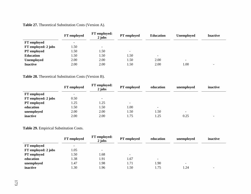
173

Table 27. Theoretical Substitution Costs (Version A).

FT employed FT employed:

2 jobs PT employed Education Unemployed Inactive

FT employed -

FT employed: 2 jobs 1.50 -

PT employed 1.50 1.50 -

Education 1.50 1.50 1.50 -

Unemployed 2.00 2.00 1.50 2.00 - Inactive 2.00 2.00 1.50 2.00 1.00 -

Table 28. Theoretical Substitution Costs (Version B).


2 jobs PT employed education unemployed inactive

FT employed -



education 1.50 1.50 1.00 -

unemployed 2.00 2.00 1.50 1.50 - inactive 2.00 2.00 1.75 1.25 0.25 -

Table 29. Empirical Substitution Costs.


2 jobs PT employed education unemployed inactive

FT employed -



education 1.38 1.91 1.67 -

unemployed 1.47 1.98 1.71 1.90 -

inactive 1.30 1.96 1.50 1.75 1.24 -

174

Cluster discrepancy and model selection

The first step in isolating the right features of the model was to calculate the pseudo-R2 for ‘cluster

discrepancy’ for all combinations of substitution costs regime, indel costs, distance measure

algorithms, and number of clusters estimated (Table 30). I estimated five, six, and seven clusters

using each dissimilarity score – a procedure commonly found in work history data by sociologists

(Biemann, Zacher & Feldman, 2012; Brzinskay-Fay, 2007). I used the Ward algorithm for cluster

analysis.

The pseudo-R2 for cluster discrepancy represents the average distance from the center of

the partition to the average distance to the overall center. A high pseudo-R2 therefore indicates a

model with clusters that are farther apart – more unique – compared to solutions with lower R2’s

(and consisting of different algorithm and cost distributions). This measure was created by Studer,

Ritschard, Gabadinho, and Müller (2011) and is available in the SADI program in Stata (Halpin,

2014). I consider this a reliable first indicator of which algorithm-cost combinations generate the

better solutions for classifying early career patterns.

Based on the pseudo-R2 criterion, I concluded that the (standard) OM algorithm generates

the highest levels of cluster discrepancy. Furthermore, across all algorithms, indels between 0.5

and 1 generally led to higher R2’s, whereby an indel of 1 achieved the highest cluster discrepancy

with an OM algorithm for five (.380), six (.401), and seven (.419) cluster solutions.

175

Table 30. Pseudo R2 of Discrepancy by Algorithm, Cost Regime, and Number of Clusters.

Equal (1) Equal (2)

5 6 7 5 6 7

HAM

no indel .241 .258 .273 .241 .258 .273

OM

indel = 0.25 .336 .359 .380 .336 .359 .380

indel = 0.5 .336 .359 .380 .336 .359 .380

indel = 0.75 .280 .301 .318 .343 .366 .385

indel = 1 .254 .276 .294 .336 .359 .380

indel = 1.25 .241 .261 .278 .310 .337 .354

indel = 1.5 .241 .260 .276 .280 .301 .318

indel = 2 .238 .255 .272 .254 .276 .294

DYN

no indel .246 .267 .284 n.a.

OMv

indel = 0.25 .206 .220 .234 .199 .215 .229

indel = 0.5 .190 .204 .216 .206 .220 .234

indel = 0.75 .171 .185 .197 .198 .215 .228

indel = 1 .166 .180 .192 .190 .204 .216

indel = 1.25 .170 .182 .193 .175 .188 .201

indel = 1.5 .161 .177 .187 .171 .185 .197

indel = 2 .162 .176 .190 .166 .180 .192

LOM

time = 0.2 / local = 0.6 .288 .309 .328 .288 .309 .328

time = 0.2 / local = 0.9 .256 .281 .299 .256 .281 .299

time = 0.4 / local = 0.4 .281 .309 .329 .281 .309 .329

time = 0.4 / local = 0.8 .250 .272 .287 .250 .272 .287

time = 0.5 / local = 0.5 .263 .283 .298 .263 .283 .298

time = 0.6 / local = 0.4 .261 .281 .296 .261 .281 .296

time = 0.6 / local = 0.8 .253 .270 .286 .253 .270 .286

time = 0.8 / local = 0.4 .249 .271 .290 .249 .271 .290

time = 0.8 / local = 0.8 .248 .264 .278 .248 .264 .278

TWED

gap = 0.2 / stiffness = 0.02 .180 .193 .206 .144 .157 .167

gap = 0.2 / stiffness = 0.06 .184 .199 .210 .147 .158 .168

gap = 0.5 / stiffness = 0.04 .232 .250 .265 .196 .209 .220

gap = 0.4 / stiffness = 0.06 .214 .230 .244 .175 .193 .206

gap = 0.6 / stiffness = 0.02 .253 .268 .282 .216 .232 .245

gap = 0.6 / stiffness = 0.06 .242 .259 .275 .208 .222 .232

176

Table 30. Pseudo R2 of Discrepancy by Algorithm, Cost Regime, and Number of Clusters. (cont.)

Theory-based (A) Theory-based (B)

5 6 7 5 6 7

HAM

no indel .290 .314 .327 .262 .274 .286

OM

indel = 0.25 .336 .359 .380 .336 .359 .380

indel = 0.5 .336 .359 .380 .336 .359 .380

indel = 0.75 .353 .376 .395 .337 .357 .375

indel = 1 .331 .349 .366 .301 .321 .337

indel = 1.25 .305 .319 .333 .274 .295 .315

indel = 1.5 .285 .305 .320 .258 .276 .293

indel = 2 .274 .289 .302 .246 .264 .278

DYN

no indel n.a. n.a.

OMv

indel = 0.25 .233 .250 .262 .202 .217 .228

indel = 0.5 .246 .265 .280 .215 .229 .241

indel = 0.75 .247 .264 .280 .208 .222 .236

indel = 1 .238 .255 .269 .195 .211 .226

indel = 1.25 .224 .242 .257 .184 .199 .212

indel = 1.5 .219 .236 .251 .191 .205 .217

indel = 2 .221 .236 .248 .186 .201 .214

LOM

time = 0.2 / local = 0.6 .332 .355 .376 .288 .312 .327

time = 0.2 / local = 0.9 .306 .326 .345 .275 .292 .308

time = 0.4 / local = 0.4 .331 .351 .371 .288 .308 .325

time = 0.4 / local = 0.8 .315 .333 .348 .269 .287 .306

time = 0.5 / local = 0.5 .320 .337 .352 .282 .298 .311

time = 0.6 / local = 0.4 .307 .332 .348 .280 .300 .313

time = 0.6 / local = 0.8 .300 .321 .337 .265 .284 .300

time = 0.8 / local = 0.4 .302 .323 .339 .272 .291 .303

time = 0.8 / local = 0.8 .290 .311 .332 .269 .284 .297

TWED

gap = 0.2 / stiffness = 0.02 .173 .185 .196 .157 .171 .181

gap = 0.2 / stiffness = 0.06 .176 .186 .196 .154 .168 .179

gap = 0.5 / stiffness = 0.04 .232 .250 .263 .210 .224 .235

gap = 0.4 / stiffness = 0.06 .214 .231 .244 .193 .212 .224

gap = 0.6 / stiffness = 0.02 .257 .271 .285 .228 .244 .258

gap = 0.6 / stiffness = 0.06 .244 .260 .271 .224 .238 .251

177

Table 30. Pseudo R2 of Discrepancy by Algorithm, Cost Regime, and Number of Clusters. (cont.)

Empirical

5 6 7

HAM

no indel .240 .259 .276

OM

indel = 0.25 .351 .374 .392

indel = 0.5 .368 .388 .406

indel = 0.75 .378 .398 .412

indel = 1 .380 .401 .419

indel = 1.25 .346 .364 .381

indel = 1.5 .315 .338 .358

indel = 2 .305 .322 .337

DYN

no indel n.a.

OMv

indel = 0.25 .198 .216 .229

indel = 0.5 .214 .227 .238

indel = 0.75 .197 .214 .227

indel = 1 .184 .199 .210

indel = 1.25 .175 .189 .201

indel = 1.5 .173 .188 .200

indel = 2 .169 .184 .198

LOM

time = 0.2 / local = 0.6 .283 .304 .323

time = 0.2 / local = 0.9 .255 .275 .292

time = 0.4 / local = 0.4 .272 .292 .309

time = 0.4 / local = 0.8 .249 .268 .283

time = 0.5 / local = 0.5 .255 .277 .292

time = 0.6 / local = 0.4 .251 .269 .287

time = 0.6 / local = 0.8 .249 .269 .283

time = 0.8 / local = 0.4 .253 .269 .282

time = 0.8 / local = 0.8 .245 .268 /.281

TWED

gap = 0.2 / stiffness = 0.02 .164 .175 .185

gap = 0.2 / stiffness = 0.06 .161 .175 .187

gap = 0.5 / stiffness = 0.04 .216 .231 .244

gap = 0.4 / stiffness = 0.06 .195 .212 .227

gap = 0.6 / stiffness = 0.02 .233 .251 .267

gap = 0.6 / stiffness = 0.06 .222 .239 .255

178

The second step, then, was to explore the qualitative features of these most cohesive

clusters within OM. Figure 11 thru 14 present the chronograms of alternatives to the selected

model (empirical substitution costs) as presented in Figure 11 of the main study: equal substitution

costs (1 and 2) and equal theory-based substitution costs (version A and B), respectively – all

within optimal matching technique. In addition, Table 31 indicates the Rand Index (Hubert &

Arabi, 1985) which is a measure of the extent to which members of a pair of cases, if in the same

cluster in one solution, are in the same cluster in the other (1 is maximum agreement).

Figure 11. Chronogram using Equal Substitution Costs (1).

Notes. Indel cost = 1, optimal matching (OM), cluster Ward.

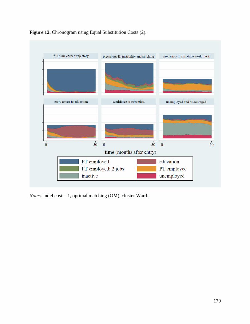
179

Figure 12. Chronogram using Equal Substitution Costs (2).


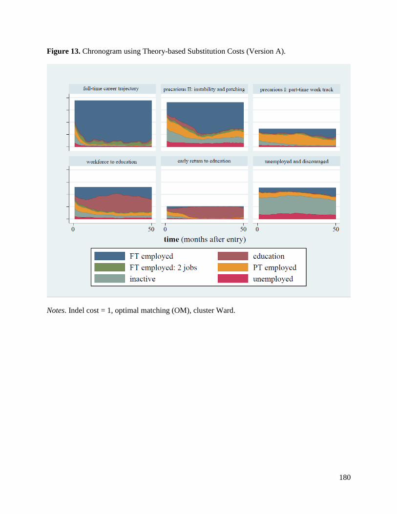
180

Figure 13. Chronogram using Theory-based Substitution Costs (Version A).


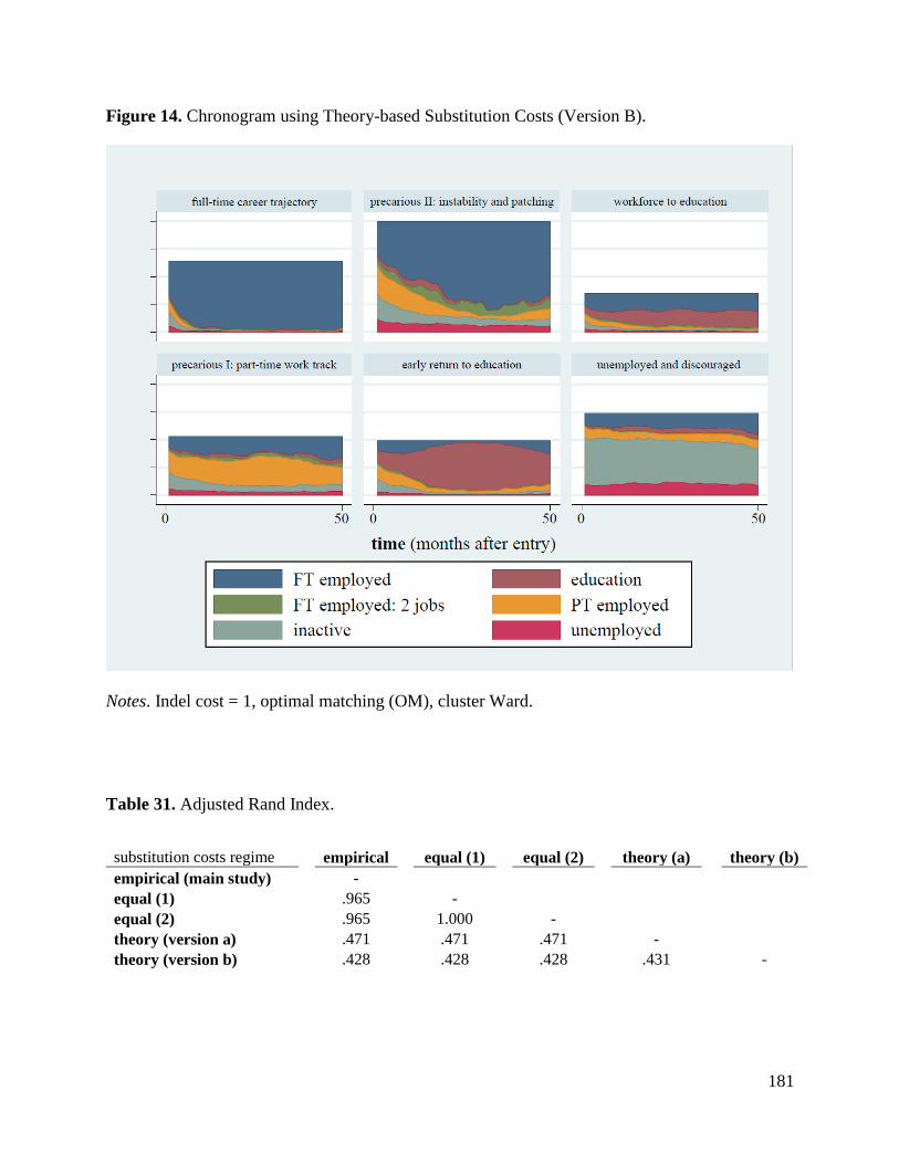
181

Figure 14. Chronogram using Theory-based Substitution Costs (Version B).


Table 31. Adjusted Rand Index.

substitution costs regime empirical equal (1) equal (2) theory (a) theory (b)

empirical (main study) - equal (1) .965 - equal (2) .965 1.000 - theory (version a) .471 .471 .471 - theory (version b) .428 .428 .428 .431 -

182

The visualization of these alternatives with different substitution costs indicates that most

solutions recognize the six clusters: early return to education, workforce to education, full-time

career trajectory, unemployed and discouraged, precarious I, and precarious II. In other words,

these competitive solutions – with less optimal quantitative features of cluster discrepancy –

display quite similar ideal types of early careers. Moreover, the Rand Index indicates that there is

not much difference in cluster assignment of cases between using empirical substitution costs and

equal substitution costs, but there is with (arbitrary) theory-based substitution costs. Taken

together, I consider the chance of wrongly assigning cases to clusters as a direct result of a

substitution costs regime to be small. I therefore kept the superior empirical substitution cost

regime, while using 1 for indels, in an optimal matching algorithm.

I finally decided that six clusters are to be preferred in this study. Although a 7-cluster

solution displays a slightly higher R2 for cluster discrepancy, the 7th cluster splits off part-time

work from the precarious I-cluster and combines this with a high risk of unemployment. I consider

this a further sub-version of the precarious I-cluster which is why I kept the ‘simpler’ 6-cluster

solution. In practice, this means that a total of 455 cases move between applying a 7-cluster

solution instead of a 6-cluster solution.

183

Conclusion.

The Role of Social Structure and Macro-Economic Conditions on Social

Inequality at Labor Market Entry.

Key Findings

Social structure within the school-to-work transition

The school-to-work transition has changed in important ways. Scholars of education and sociology

have documented the increasing complexity of delayed school leaving, delayed college enrollment,

delayed time to degree, stopping out, and reenrollment to complete a degree or to obtain a post-

graduate degree. Together, these patterns prove the outdatedness of the so-called triphasic life

course: education to the work career to retirement. More precisely, the transition from education

to work can no longer be simplified into a one-time event.

The four empirical studies in this dissertation have attempted to draw attention to different

components of today’s labor market entry phase. These studies address the changing character of

this phase by analyzing the school-to-work pathway for different cohorts of high school students

(ages 16 to 25), with birth cohorts ranging between the 1960s to 1989. After harmonizing these

pathways, comparative analyses were conducted with data from four countries: the United States,

the United Kingdom, Germany, and Sweden. Of primary concern was whether the school-to-work

trajectories in these countries have been changing in the same direction. In addition, the cross-

184

national comparisons examine whether the distinct features of the four educational systems and

the labor markets can be associated with different stratification mechanisms, perceived as a

process rather than an event.

In the first chapter of this dissertation, sequence analysis was introduced as one promising

methodology to advance knowledge about trajectories rather than transitions. It allows researchers

to examine the pathway from school to work holistically and to reveal the inequalities within some

of them. This technique was applied in the most innovative form in Chapter 3. From a

methodological point of view, it connects the clustering of ideal-typical sequences with long-term

labor market outcomes of school leavers. Chapter 5 reviews the methodological discussions around

social sequence analyses as well as how new versions of the algorithm yield slightly different

results. Above all, Chapter 5 demonstrates that there is (still) no consensus as to which type of

sequence alignment techniques best capture social processes. However, the results reported in the

analysis underwent rigorous robustness checks. Tweaking the cost distributions did not produce

radically different typologies of pathways and some matching algorithms yielded better

cohesiveness of the clusters than others did.

Using the descriptive statistics of sequence analysis, Chapter 1 showed that the United

States has been surpassed by at least some countries in giving access to continuous higher

education attainment. Over time, students’ ten-year trajectory from high school (age 16) to their

mid-twenties consist of more full-time education attendance in the United States, the United

Kingdom, Germany, and Sweden. Moreover, the pathway from education to the labor market has

become more alike across these four countries in certain ways. Over time, the early careers of

recent school leavers have become slightly more stable in the United States – a liberal welfare state

– while labor market pathways in the only social-democratic country in this study (Sweden) seem

185

to become slightly more insecure and volatile. Between these four ideal-typical welfare state

regimes, these outcomes provide some support to theories of welfare state convergence.

More importantly, this study went back to a forgotten part of welfare state studies: the

educational system and its connection to early labor market stratification. The school-to-work

transition is currently understood as a single event in both educational theory through the

classification of educational systems and labor market theory through the distinction between types

of human capital acquisition and payoffs. However, the idea of a life course phase as opposed to a

one-time event draws attention to a trajectory in which students face several structures of the

welfare state. First, the school system itself is a function of a public vs. private distribution of

resources and costs. A completely public and free educational system is a universal policy, rather

than particularistic, and therefore has an equalizing effect on opportunities. Second, similarly

educated school leavers face different labor market insecurities and different safety nets across

different countries. These structures can be understood from a welfare state regime lens. Students

and young labor market entrants in different nations vary in the extent to which they are dependent

on the erratic character of the labor market and the protection available from social security or

(public) education options. As such, the extent to which young individuals do or do not experience

insecurity, due to different levels of policy and social structure, can (and should) be considered a

form of de-commodification.

The analyses of Chapter 1 showed that in each country a substantial proportion of

individuals face job precarity and instability in the school-to-work transition phase. While

precarious work applies to an employment position that is nonstandard and insecure, often

consisting of part-time work, doubling-up jobs, and night shifts, my analysis suggests that certain

groups of young individuals are stuck in precarious early careers. This concept entails a longer

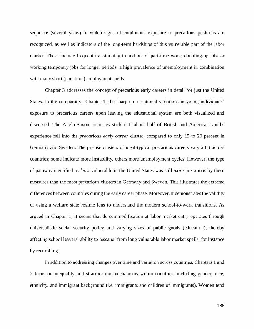
186

sequence (several years) in which signs of continuous exposure to precarious positions are

recognized, as well as indicators of the long-term hardships of this vulnerable part of the labor

market. These include frequent transitioning in and out of part-time work; doubling-up jobs or

working temporary jobs for longer periods; a high prevalence of unemployment in combination

with many short (part-time) employment spells.

Chapter 3 addresses the concept of precarious early careers in detail for just the United

States. In the comparative Chapter 1, the sharp cross-national variations in young individuals’

exposure to precarious careers upon leaving the educational system are both visualized and

discussed. The Anglo-Saxon countries stick out: about half of British and American youths

experience fall into the precarious early career cluster, compared to only 15 to 20 percent in

Germany and Sweden. The precise clusters of ideal-typical precarious careers vary a bit across

countries; some indicate more instability, others more unemployment cycles. However, the type

of pathway identified as least vulnerable in the United States was still more precarious by these

measures than the most precarious clusters in Germany and Sweden. This illustrates the extreme

differences between countries during the early career phase. Moreover, it demonstrates the validity

of using a welfare state regime lens to understand the modern school-to-work transitions. As

argued in Chapter 1, it seems that de-commodification at labor market entry operates through

universalistic social security policy and varying sizes of public goods (education), thereby

affecting school leavers’ ability to ‘escape’ from long vulnerable labor market spells, for instance

by reenrolling.

In addition to addressing changes over time and variation across countries, Chapters 1 and

2 focus on inequality and stratification mechanisms within countries, including gender, race,

ethnicity, and immigrant background (i.e. immigrants and children of immigrants). Women tend

187

to be more exposed to precarious pathways than men. Even after controlling for marital status and

having children, women are much more likely to experience job precarity through moving in and

out of part-time work and unemployment. However, more research is needed to unpack these

gender differences within and across countries because the gender effect ceases to be significant

in some countries.

Furthermore, the analysis for just the United States incorporates parental background

(Chapter 3), showing that both parental social class and race/ethnicity are highly predictive of

being routed into precarious early careers. Black Americans in United States are structurally

disadvantaged in comparison to whites as they are significantly more likely to experience precarity

in the labor market. This finding is robust to educational level, which is by far the best predictor

of early career instability. Job market entrants with a college degree are significantly more likely

to experience a stable full-time pathway in the first years in the labor market, while high school

dropouts and high school graduates lack this protection.

Timing and inequality

During the revision process of one chapter of this dissertation and the presentation of the results

of several chapters at conferences, some scholars’ immediate reaction to precarious early careers

was; “Aren’t young people who first enter the labor market not just figuring out which profession

suits them best?” In other words, the careers of young individuals who transition from school to

work may look precarious, but they are actually a natural component of job matching.

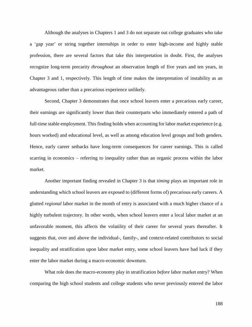
188

Although the analyses in Chapters 1 and 3 do not separate out college graduates who take

a ‘gap year’ or string together internships in order to enter high-income and highly stable

profession, there are several factors that take this interpretation in doubt. First, the analyses

recognize long-term precarity throughout an observation length of five years and ten years, in

Chapter 3 and 1, respectively. This length of time makes the interpretation of instability as an

advantageous rather than a precarious experience unlikely.

Second, Chapter 3 demonstrates that once school leavers enter a precarious early career,

their earnings are significantly lower than their counterparts who immediately entered a path of

full-time stable employment. This finding holds when accounting for labor market experience (e.g.

hours worked) and educational level, as well as among education level groups and both genders.

Hence, early career setbacks have long-term consequences for career earnings. This is called

scarring in economics – referring to inequality rather than an organic process within the labor

market.

Another important finding revealed in Chapter 3 is that timing plays an important role in

understanding which school leavers are exposed to (different forms of) precarious early careers. A

glutted regional labor market in the month of entry is associated with a much higher chance of a

highly turbulent trajectory. In other words, when school leavers enter a local labor market at an

unfavorable moment, this affects the volatility of their career for several years thereafter. It

suggests that, over and above the individual-, family-, and context-related contributors to social

inequality and stratification upon labor market entry, some school leavers have bad luck if they

enter the labor market during a macro-economic downturn.

What role does the macro-economy play in stratification before labor market entry? When

comparing the high school students and college students who never previously entered the labor

189

market, Chapter 2 showed that in most situations of macro-economic downturns while enrolled

(high unemployment or recession), students are less likely to enter the labor market; they stay in

school longer, ceritus paribus, and therefore avoid the turbulent and volatile experience in the

early career. In other words, students are encouraged to stay in education for a bit longer. However,

the opposite is true for high school students in the United States. They are more likely to enter the

labor market for the first time when the economy is in a recession and the unemployment rate is

high. Economists call this a ‘discouraged student effect’ of unfavorable macro-economic

conditions because students may reduce their perceived value of completing high school.

Chapters 2 and 4 also consider the macro-economic conditions, but only for those

individuals who have just entered the labor market. Among school leavers in the United States

who did not complete high school or who did not complete a higher education degree (and

therefore have most to gain for educational reentry), both an economic recession and a high

unemployment reduce the probability of reenrollment. School leavers in the United Kingdom,

Germany, and Sweden showed either no response to macro-conditions or the expected increased

probability of ‘human capital catch-up.’ In addition, when American school leavers face

difficulties in their own early career phase (i.e. a high number of unemployment spells), they also

seem less likely to return to the educational system. In contrast, those who already have above-

average earnings and occupational statuses (SEI) are more likely to reenroll, and more so during a

recession.

Together, these findings regarding school leaving and reenrollment have three important

implications for a sociological understanding of school-to-work trajectories. First, macro-

economic downturns leading to less investment in education among the vulnerable group of

students and school leavers in the United States contradicts Human Capital Theory. More

190

specifically, it shows that youths become more risk averse as a direct consequence of economic

shocks such as a recession. The analyses in these studies cannot address individual-level

incentives. More research is needed to understand how broader socio-economic forces affect

school-and career decision-making of young individuals. However, it is clear that the rationality

assumption is insufficient to explain the changing school leaving and reenrollment pace of some

groups.

Second, macro-economic conditions increase inequality between groups, most primarily

between the lower- and higher-educated. Not only are lower-educated more likely to experience

precarity during the early career, regardless of timing and context, this risk further increases in

response to high unemployment and recessions in the United States. Students and school leavers

who are most vulnerable in the labor market do not have the same chance to benefit from

educational investment and educational refreshing. This process of inequality is not visible in the

aggregate measures of the relationship between the economy and educational enrollment – these

portray an image of higher enrollments during recessions across educational levels. However,

when focusing on individual-level longitudinal data, the hidden inequalities between groups come

to the fore.

Third, risk-aversion regarding school leaving or reentry and exposure to precarious early

careers is much higher in the United States (and to some extent the United Kingdom) than in

Germany and Sweden. This study did not directly observe the consequences of specific policies.

However, if we were to better understand the cross-national differences between these four ideal-

typical welfare states, these findings suggest that traditional corporatist regimes and social-

democratic regimes have built more layers of protection that mitigate risk aversion in the school-

to-work trajectory.

191

Future research

The findings from this dissertation generate a few new research questions. Here, the longitudinal

perspective on precarious work – precarious careers – applies to the phase immediately upon labor

market entry. Trajectories of precarious work are however likely to appear throughout in the mid-

and late-career albeit in different forms. One recent example of a more comprehensive approach

to precarious work is Kalleberg’s (2018) recently published study called Precarious Lives. This

book takes a broader life-course perspective of nonstandard work and career instability by

comparing the transition to adulthood, family formation, and happiness in the United States, the

United Kingdom, Germany, Japan, Spain, and Denmark.

The complexity of reenrollment, in particular during recessions, also requires more

sociological research to inform policy-making. Educational reenrollment is generally considered

as the best rational choice if a young school leaver is exposed to precarious work and

unemployment cycles or enters the labor force during a recession. However, more empirical

research is needed to understand under what conditions and for which groups such an educational

reenrollment actually pays off. Table 32 is an example of how this type of research can be

conducted. It shows the average treatment effect of educational reentry among similarly educated

school leavers during a recession for both the United States and the United Kingdom. The

counterfactual of the binary ‘reenrollment’ treatment is staying in the labor force throughout the

recession. This particular regression adjusts for selection into treatment (reenrollment) and

suggests that reenrollment during a recession has a substantial earnings payoff for higher education

attendees in the United States. No significant benefit was found in the UK or for lower-educated

Americans.

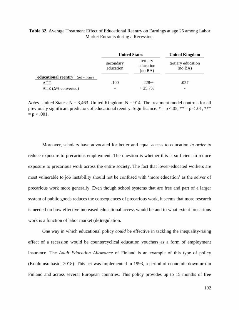
192

Table 32. Average Treatment Effect of Educational Reentry on Earnings at age 25 among Labor

Market Entrants during a Recession.


secondary

education

tertiary

education

(no BA)

tertiary education

(no BA)

educational reentry 1 (ref = none)

ATE .100 .228** .027

ATE (∆% converted) - + 25.7% -

Notes. United States: N = 3,463. United Kingdom: N = 914. The treatment model controls for all

previously significant predictors of educational reentry. Significance: * = p <.05, ** = p < .01, ***

= p < .001.

Moreover, scholars have advocated for better and equal access to education in order to

reduce exposure to precarious employment. The question is whether this is sufficient to reduce

exposure to precarious work across the entire society. The fact that lower-educated workers are

most vulnerable to job instability should not be confused with ‘more education’ as the solver of

precarious work more generally. Even though school systems that are free and part of a larger

system of public goods reduces the consequences of precarious work, it seems that more research

is needed on how effective increased educational access would be and to what extent precarious

work is a function of labor market (de)regulation.

One way in which educational policy could be effective in tackling the inequality-rising

effect of a recession would be countercyclical education vouchers as a form of employment

insurance. The Adult Education Allowance of Finland is an example of this type of policy

(Koulutusrahasto, 2018). This act was implemented in 1993, a period of economic downturn in

Finland and across several European countries. This policy provides up to 15 months of free

193

education for individuals who already transitioned from school to work. Depending on one’s

previous salary it also guarantees an allowance of about 60 percent of the previously held salary.

This type of educational policy not only incentivizes human capital investment among young

adults, it serves as a protection mechanism for lower-educated workers in particular at times when

labor surplus is increasing.

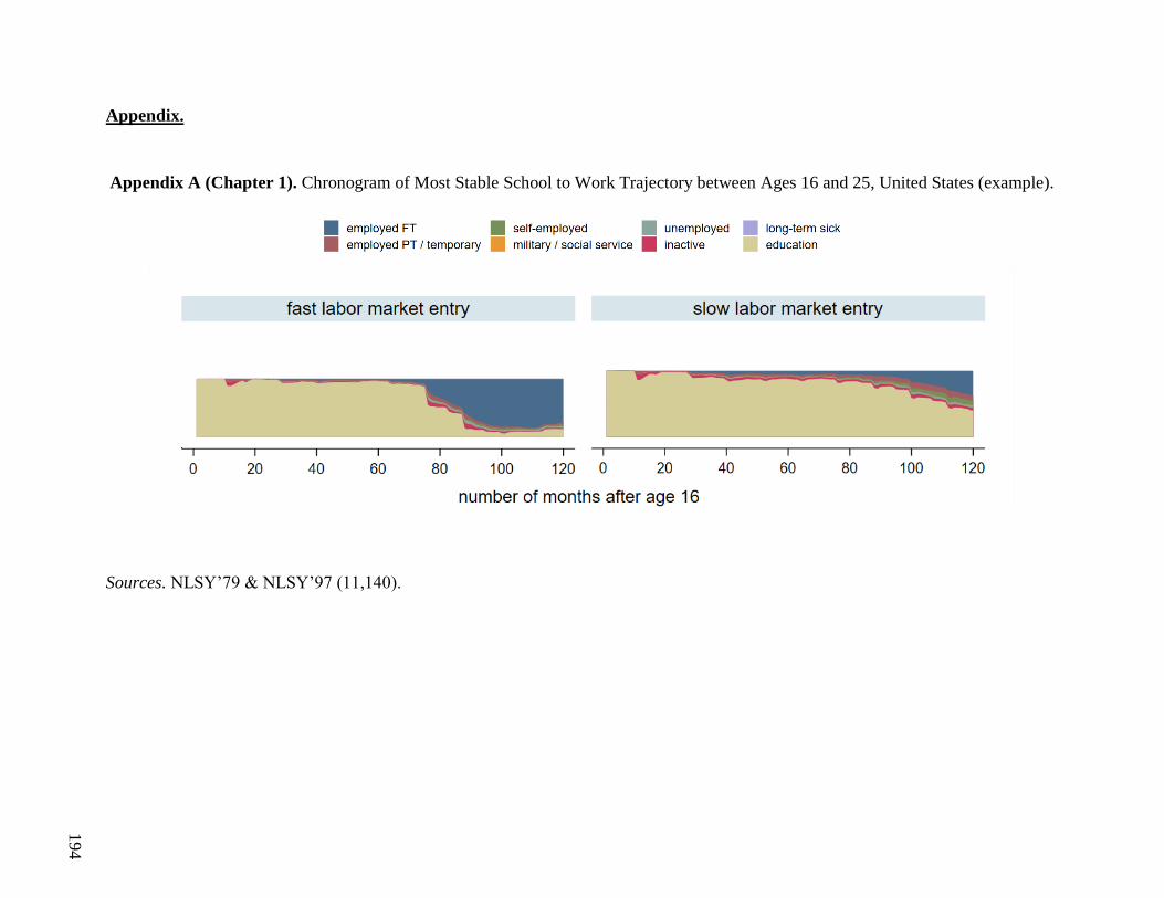
194

Appendix.

Appendix A (Chapter 1). Chronogram of Most Stable School to Work Trajectory between Ages 16 and 25, United States (example).

Sources. NLSY’79 & NLSY’97 (11,140).

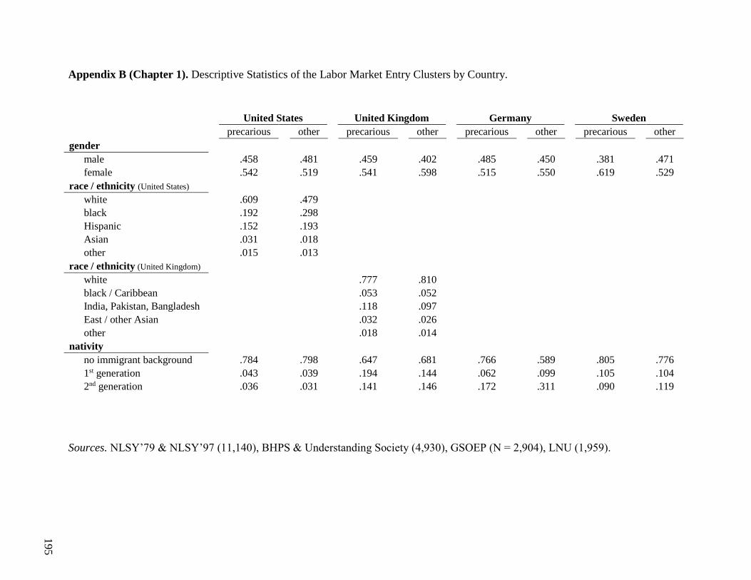
195

Appendix B (Chapter 1). Descriptive Statistics of the Labor Market Entry Clusters by Country.

United States United Kingdom Germany Sweden precarious other precarious other precarious other precarious other

gender

male .458 .481 .459 .402 .485 .450 .381 .471 female .542 .519 .541 .598 .515 .550 .619 .529

race / ethnicity (United States)

white .609 .479

black .192 .298

Hispanic .152 .193

Asian .031 .018

other .015 .013

race / ethnicity (United Kingdom)

white .777 .810

black / Caribbean .053 .052

India, Pakistan, Bangladesh .118 .097

East / other Asian .032 .026

other .018 .014

nativity

no immigrant background .784 .798 .647 .681 .766 .589 .805 .776 1st generation .043 .039 .194 .144 .062 .099 .105 .104 2nd generation .036 .031 .141 .146 .172 .311 .090 .119


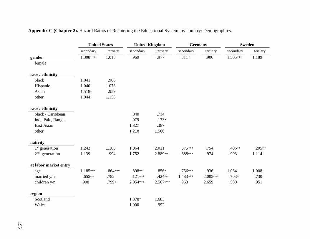
196

Appendix C (Chapter 2). Hazard Ratios of Reentering the Educational System, by country: Demographics.

United States United Kingdom Germany Sweden secondary tertiary secondary tertiary secondary tertiary secondary tertiary

gender 1.308*** 1.018 .969 .977 .811* .906 1.505*** 1.189 female

race / ethnicity

black 1.041 .906

Hispanic 1.040 1.073

Asian 1.518* .959

other 1.044 1.155

race / ethnicity

black / Caribbean .840 .714

Ind., Pak., Bangl. .979 .173*

East Asian 1.327 .387

other 1.218 1.566

nativity

1st generation 1.242 1.103 1.064 2.011 .575*** .754 .406** .205** 2nd generation 1.139 .994 1.752 2.889** .688*** .974 .993 1.114

at labor market entry

age 1.185*** .864*** .898** .856* .756*** .936 1.034 1.008 married y/n .655** .782 .121*** .424** 1.483*** 2.005*** .703* .730 children y/n .908 .799* 2.054*** 2.567*** .963 2.659 .580 .951

region

Scotland 1.378* 1.683

Wales 1.000 .992

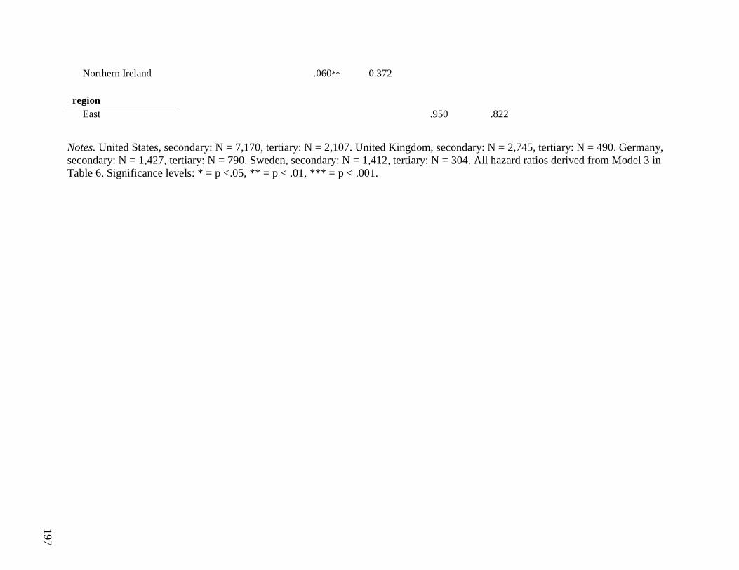
197

Northern Ireland .060** 0.372

region

East .950 .822

Notes. United States, secondary: N = 7,170, tertiary: N = 2,107. United Kingdom, secondary: N = 2,745, tertiary: N = 490. Germany,

secondary: N = 1,427, tertiary: N = 790. Sweden, secondary: N = 1,412, tertiary: N = 304. All hazard ratios derived from Model 3 in

Table 6. Significance levels: * = p <.05, ** = p < .01, *** = p < .001.

198

References

Abbott, A. & Forrest, J. (1986). Optimal matching methods for historical sequences. The Journal

of Interdisciplinary History, 16(3), 471 – 494.

Abbott, A. & Hrycak, A. (1990). Measuring resemblance in sequence data: An optimal matching

analysis of musicians' careers. American Journal of Sociology, 96(1), 144 – 185.

Achterberg, P. & Yerkes, M. (2009). One welfare state emerging? Convergence versus divergence

in 16 western countries. Journal of Comparative Social Welfare, 25(3), 189 – 201.

Addison, J.T. & Surfield, C.J. (2009). Atypical work and employment continuity. Industrial

Relations: A Journal of Economy and Society, 48(4), 655 – 683.

Aisenbrey, S. & Fasang, A.E. (2010). New life for old ideas: The ‘second wave’ of sequence

analysis bringing the ‘course’ back into the life course. Sociological Methods & Research,

38(3), 420 – 462.

Alexander, K., Bozick, R. & Entwisle, D. (2008). Warming up, cooling out, or holding steady?

Persistence and change in educational expectations after high School. Sociology of

Education 81(4), 371 – 396.

Allmendinger, J. (1989). Educational systems and labor market outcomes. European Sociological

Review, 5, 231 – 250.

Anyadike-Danes, M. & McVicar, D. (2005). You'll never walk alone: Childhood influences and

male career path clusters. Labour Economics, 12(4), 511 – 530.

Anyadike-Danes, M. & McVicar, D. (2010). My brilliant career: Characterizing the early labor

market trajectories of British women from Generation X. Sociological Methods &

Research, 38(3), 482 – 512.

https://www.tandfonline.com/toc/rjcs20/current

199

Arum, R. & Shavit, Y. (1995). Secondary vocational education and the transition from school to

work. Sociology of Education, 68, 187 – 204.

Asteriou, D. & Agiomirgianakis, G.M. (2001). Human capital and economic growth: Time series

evidence from Greece. Journal of Policy Modeling, 23(5), 481 – 489.

Astone, N.M., Schoen, R., Ensminger, M. & Rothert, K. (2000). School reentry in early adulthood:

The case of inner-city African Americans. Sociology of Education, 73(3), 133 –154.

Autor, D.H. & Houseman, S.N. (2010). Do temporary-help jobs improve labor market

outcomes for low-skilled workers? Evidence from "Work First". American Economic

Journal: Applied Economics, 2(3), 96 – 128.

Barone, C. & Schizzerotto, A. (2011). Introduction: Career mobility, education, and

intergenerational reproduction in five European societies. European Societies, 13(3), 331

– 345.

Barr, A. & Turner, S.E. (2013). Expanding enrollments and contracting state budgets: The effect

of the Great Recession on higher education. The ANNALS of the American Academy of

Political and Social Science, 650(1), 168 – 193.

Becker, G.S. (1964). Human capital: A theoretical and empirical analysis, with

special reference to education. Chicago: University of Chicago Press.

Bernhardt, A., Morris, M., Handcock, M.S., & Scott, M.A. (2001). Divergent paths: Economic

mobility in the new American labor market. New York: Russell Sage Foundation.

Betts, J.R. & McFarland, L.L. (1995). Safe port in a storm: The impact of labor market conditions

on community college enrollments. Journal of Human Resources, 30(4), 741 – 765.

Beutner, M. & Pechuel, R. (2017). Education and educational policy in Germany. A focus on core

developments since 1944. Italian Journal of Sociology of Education, 9(2), 9 – 24.

200

Biemann, T., Zacher, H. & Feldman, D.C. (2012). Career patterns: A twenty-year panel study.

Journal of Vocational Behavior, 81(2), 159 – 170.

Blanchard, P., Bühlmann, F. & Gauthier, J. (2014). Advances in sequence analysis: Theory,

method, applications (Edited Volume, 2). New York: Springer.

Blossfeld, H., Buchholz, S., Bukodi, E., & Kurz, K. (2009). Young workers, globalization and

the labor market: Comparing early working life in eleven countries. (Edited Volume).

Cheltenham: Edward Elgar.

Boisjoly, J., Duncan, G.J., & Smeeding, T. (1998). The shifting incidence of involuntary job losses

from 1968 to 1992. Industrial relations: A journal of economy and society, 37(2), 207 –

231.

Bol, T. & Van de Werfhorst, H.G. (2011). Signals and closure by degrees: The education effects

across 15 European Countries. Research in Social Stratification and Mobility, 29, 119 –

132.

Bol, T. & Van de Werfhorst, W.G. (2013). Educational systems and the trade-off between labor

market allocation and equality of educational opportunity. Comparative Education Review,

57(2): 285 – 308.

Boudon, R. (1974). Education, inequality and social opportunity. New York: Wiley.

Brauns, H., Steinmann, S., Kieffer, A., & Marry, C. (1999). Does education matter? France and

Germany in comparative perspective. European Sociological Review, 15, 61 – 90.

Breen, R. (1997). Risk, recommodification, and stratification. Sociology, 31(3), 473 – 489.

Breen, R. & Buchmann, M. (2002). Institutional variation in youth unemployment: Market and

institutional factors. Annals of the American Academy, 580, 288 – 305.

201

Breen, R., Luijkx, R., Müller, W. & Pollak R. (2009). Nonpersistent inequality in educational

attainment: evidence from eight European countries. American Journal of Sociology,

114(5), 1475 – 1521.

Brint, S. (1998). Schools and societies. Thousand Oaks: Pine Forge Press.

Brint, S. & Karabel, J. (1989). American education, meritocratic ideology, and the legitimation of

inequality: The community college and the problem of American exceptionalism. Higher

Education, 18(6), 725 – 735.

Brint, S. & Karabel, J. (1989). The Diverted Dream: Community Colleges and the Promise of

Educational Opportunity in America, 1900-1985. Oxford: Oxford University Press.

Brown, D.K. (2001). The social sources of educational credentialism: Status cultures, labor

markets and organizations. Sociology of Education, 74, 19 – 34.

Brückner, H. & Mayer, K.U. (2005). De-standardization of the life course: What it might mean?

And if it means anything, whether it actually took place? Advances in Life Course

Research, 9, 27 – 53.

Brzinsky-Fay, C. (2007). Lost in transition? Labour market entry sequences of school leavers in

Europe. European Sociological Review, 23(4), 409 – 422.

Brzinsky-Fay, C. (2014). The measurement of school-to-work transitions as processes: About

Events and Sequences. European Societies, 16(2), 213 – 232.

Brzinsky-Fay, C. & Kohler, U. (2010). New developments in sequence analysis. Sociological

Methods & Research, 38(3), 359 – 364.

Bureau of Labor Statistics, U.S. Department of Labor. (2014). National Longitudinal Survey of

Youth 1979 cohort, 1979-2012 (rounds 1-25). Columbus: Center for Human Resource

Research, The Ohio State University.

202

Bureau of Labor Statistics, U.S. Department of Labor. (2015). National Longitudinal Survey of

Youth 1997 cohort, 1997-2013 (rounds 1-16). Columbus: Center for Human Resource

Research, The Ohio State University.

Cabus, S.J. & De Witte, K. (2012). Naming and shaming in a ‘fair’ way. On disentangling the

influence of policy in observed outcome. The Journal of Policy Modeling, 34(5), 767 –

787.

Cabus, S.J. & De Witte, K. (2016). Why do students leave education early? Theory and evidence

on high school dropout rates. The Journal of Forecasting, 35(8), 690 – 702.

Camey, S.A., Torman, V.B.L., Hirakata, V.N., Cortes, R.X., Vigo, A. (2014). Bias of using odds

ratio estimates in multinomial logistic regressions to estimate relative risk or prevalence

ratio and alternatives. Cadernos de Saúde Pública, 30(1), 21 – 29.

Card, D. & Lemieux, T. (2001). Dropout and enrollment trends in the postwar period: What went

wrong in the 1970s? In J. Gruber, Risky Behavior among Youths: An Economic Analysis

(pp. 439 – 482). Chicago: Chicago University Press.

Chauvel, L. (2010). The long-term destabilization of youth, scarring effects, and the future of

the welfare regime in post-trente glorieuses France. French Politics, Culture & Society,

28(3), 74 – 96.

Clark, B.R. (1960). The "cooling-out" function in higher education. American journal of

Sociology, 65(6), 569 – 576.

Clark, B.R. (1980). The "cooling-out" function revisited. New Directions for Community Colleges,

32, 15 – 31.

Clark, D. (2011). Do recessions keep students in school? The impact of youth unemployment on

enrolment in post‐compulsory education in England. Economica, 78(311), 523 – 545.

http://www.berghahnjournals.com/view/journals/fpcs/fpcs-overview.xml

http://www.berghahnjournals.com/view/journals/fpcs/fpcs-overview.xml

203

Cohn, A., Engelmann, J., Fehr, E. & Maréchal, M.A. (2015). Evidence for countercyclical risk

aversion: An experiment with financial professionals. The American Economic Review,

105(2), 860 – 885.

Cornwell, B. (2015). Social Sequence Analysis. Methods and Applications. New York: Cambridge

University Press.

Corrales-Herrero, H. & Rodríguez-Prado, B. (2012). Characterizing Spanish labour pathways of

young people with vocational lower-secondary education. Applied Economics, 44(29),

3777 – 3792.

Cox, D.R. (1972). Regression models and life-tables (with discussion). Journal of the Royal

Statistical Society, Series B, 34, 187 – 220.

Crofton, S.O., Anderson, W.L. & Rawe, E.C. (2009). Do higher real minimum wages lead to more

high school dropouts? Evidence from Maryland across races, 1993–2004. American

Journal of Economics and Sociology, 68(2), 445 – 464.

De Witte, K., Nicaise, I., Lavrijsen, J., Van Landeghem, G. , Lamote, C. & Van Damme, J. (2013)

The impact of institutional context, education and labour market policies on early school

leaving: A comparative analysis of EU countries. European Journal of Education, 48, 331

– 345.

DesJardins, S.L., Ahlburg, D.A. & McCall, B.P. (2006). An integrated model of application,

admission, enrollment, and financial Aid. The Journal of Higher Education, 77(3), 381 –

429.

Deterding, N.M. (2015). Instrumental and expressive education: College planning in the face of

poverty. Sociology of Education, 88(4), 284 – 301.

204

DiPrete, T.A. (1993). Industrial restructuring and the mobility response of American workers in

the 1980s. American Sociological Review, 58(1), 74 – 96.

DiPrete, T.A. (2005). Labor markets, inequality, and change: A European perspective. Work and

Occupations, 32(2), 119 – 139.

DiPrete, T.A., Eller C.C., Bol T. & Van de Werfhorst, W.G. (2017). School-to-work linkages in

the United States, Germany, and France. American Journal of Sociology, 122(6), 1869 –

1938.

DiTomaso, N. (2001). The loose coupling of jobs. In I. Berg & A. Kalleberg (Eds.), Sourcebook

of labor markets (pp 247-270). New York: Springer US.

Dougherty, K.J. (1994). The contradictory college: The conflicting origins, impacts, and futures

of the community college. Albany: SUNY Press.

Elman, C. & O'Rand, A. (1998). Midlife entry into vocational training: A mobility model. Social

Science Research, 27(2), 128 – 158.

Elman, C. & O'Rand, A. (2002). Perceived job insecurity and entry into work-related education

and training among adult workers. Social Science Research, 31(1), 49 – 76.

Elman, C. & O'Rand, A. (2004). The race is to the swift: Socioeconomic origins, adult education,

and wage attainment. American Journal of Sociology, 110(1), 123 – 60.

Elman, C. & O'Rand, A. (2007). The effects of social origins, life events, and institutional sorting

on adults’ school transitions. Social Science Research, 36(3), 1276 – 1299.

Esping-Andersen, G. (1990). Three worlds of welfare capitalism. Princeton: Princeton University

Press.

Esping-Andersen, Gøsta. (1999). Social foundations of postindustrial economies. Oxford: Oxford

University Press.

205

Estevez-Abe, M., Iversen, T. & Soskice, D. (2001). Social protection and the formation of skills:

A reinterpretation of the welfare state. In P.A. Hall and D. Soskice (Eds.), Varieties of

Capitalism. The Institutional Foundations of Comparative Advantage (pp. 145-183).

Oxford: Oxford University Press.

Feldman, D.C. & Doerpinghaus, H.I. (1992). Patterns of part-time employment. Journal of

Vocational Behavior, 41(3), 282 – 294.

Fouarge, D., Manzoni, A., Muffels, R., & Luijkx, R. (2010). Childbirth and cohort effects on

mothers' labour supply: A comparative study using life history data for Germany, the

Netherlands and Great Britain. Work, Employment & Society, 24(3), 487 – 507.

Fry, R. (2009). College enrollment hits all-time high, fueled by community college surge.

Washington, DC: Pew Research Center Publications.

Gangl, M. (2003). The structure of labour market entry in Europe: A typological analysis. In W.

Müller (Ed.), Transitions from education to work in Europe (pp. 95-116). Oxford: Oxford

University Press.

Gangl, M. (2006). Scar effects of unemployment: An assessment of institutional

complementarities. American Sociological Review, 71(6), 986 – 1013.

Ghilani, M.E. (2008). Displaced workers successfully reenter the workforce: Post-graduation from

a community college. Community college journal of research and practice, 32(8), 573 –

581.

Goldrick-Rab, S. (2006). Following their every move: An investigation of social-class differences

in college pathways. Sociology of Education, 79(1), 67 – 79.

Goldrick-Rab, S. & Han, S.W. (2011). Accounting for socioeconomic differences in delaying the

transition to college. The Review of Higher Education, 34(3), 423 – 445.

206

Greenwood, M.J. (2014). Migration and economic growth in the United States: National,

regional, and metropolitan perspectives. New York: Academic Press.

Grimshaw, D., Ward, K.G., Rubery J., & Beynon, H. (2001). Organisations and the

transformation of the internal labour market. Work, Employment and Society, 15(1), 25 –

54.

Hacker, J.S. (2006). The Great Risk Shift: The New Economic Insecurity and the Decline of the

American Dream. New York: Oxford University Press.

Halpin, B. (2010). Optimal matching analysis and life course data: The importance of duration.

Sociological Methods & Research, 38(3), 365 – 388.

Halpin, B. (2012). Multiple imputation for life-course sequence data. Retrieved from

teaching.sociology.ul.ie/seqanal/shortptex.pdf

Halpin, B. (2017). SADI: Sequence analysis tools for Stata. The Stata Journal, 17(3), 546 – 572.

Hamming, R.W. (1950). Error detecting and error correcting codes. Bell System Technical Journal,

29(2), 147 – 160.

Harbison, F. & Myers, C. (1964). Education, manpower, and economic growth. New York:

McGraw-Hill.

Hartman, S. (2007). The development of the Swedish educational system. In M. Carlson, A. Rabo

& F. Gök (Eds.), Education in ’multicultural’ societies. Turkish and Swedish perspectives,

London: I.B. Tauris.

Hearn, J.C. (1992). Emerging variations in postsecondary attendance patterns: An investigation of

part-time, delayed, and nondegree enrollment. Research in Higher Education, 33(6), 657

– 687.

207

Hega, G.M. & Hokenmaier, K.G. (2002). The welfare state and education: A comparison of social

and educational policy in advanced industrial societies. German Policy Studies, 2(1), 1 –

29.

Home, A.M. (1998). Predicting role conflict, overload and contagion in adult women university

students with families and jobs. Adult Education Quarterly, 48(2), 85 – 97.

Hollister, M. (2009). Is optimal matching suboptimal? Sociological Methods & Research, 38(2),

235 – 264.

Hollister, M. (2011). Employment stability in the US labor market: Rhetoric versus reality.

Annual Review of Sociology, 37, 305 – 324.

Hopper, E.I. (1968). A typology for the classification of educational systems. Sociology, 2(29), 29

– 46.

Hubert, L. & Arabie, P. (1985). Comparing partitions. Journal of Classification, 2(1), 193 – 218.

Ianelli, C. & Raffe, D. (2007). Vocational upper-secondary education and the transition from

school. European Sociological Review, 23, 49 – 63.

Iversen,T. & Stephens, J.D. (2008). Partisan politics, the welfare state, and three worlds of human

capital formation. Comparative Political Studies, 41, 600 – 627.

Jacob, M. & Weiss, F. (2010). From higher education to work patterns of labor market entry in

Germany and the US. Higher Education, 60(5), 529 – 542.

Kalleberg, A.L. (2009). Precarious work, insecure workers: Employment relations in transition.

American Sociological Review, 74(1), 1 – 22.

Kalleberg, A.L. (2000). Nonstandard employment relations: Part-time, temporary and contract

work. Annual Review of Sociology, 26, 341 – 365.

208

Kalleberg, A.L. (2011). Good jobs, bad jobs. The rise of polarized and precarious employment

systems in the United States, 1970s to 2000s. New York: Russell Sage Foundation.

Kalleberg, A.L. (2012). Job quality and precarious work clarifications, controversies, and

challenges. Work and Occupations, 39(4), 427 – 448.

Kalleberg, A.L., Reskin, B.F., & Hudson, K. (2000). Bad jobs in America: Standard and

nonstandard employment relations and job quality in the United States. American

Sociological Review, 65(2), 256 – 278.

Kasworm, C.E. (1993). Adult higher education from an international perspective. Higher

Education, 25(4), 411 – 423.

Kasworm, C.E. (1993). An alternative perspective on empowerment of adult undergraduates.

Contemporary Education, 64(3), 162 – 165.

Kerckhoff, A.C. (1996). Building conceptual and empirical bridges between studies of educational

and labour force careers. In A.C. Kerckhoff, Generating social stratification: Toward a

new research agenda (pp. 37 – 56). Boulder: Westview Press.

Kerckhoff, A.C. (2001). Education and social stratification processes in comparative perspective.

Sociology of Education, 74, 3 – 18.

Kerckhoff, A.C. & Glennie, E. (1999). The Matthew effect in American education. Research in

Sociology of Education and Socialization, 12(1), 35 – 66.

Kimmel, S.B. & Neese, M.N. (2006). Barriers to business education: Motivating adult learners.

Journal of Behavioral and Applied Management, 7(3), 292 – 303.

Kletzer, L.G. & Fairlie, R.W. (2003). The long-term costs of job displacement for young adult

workers. Industrial & Labor Relations Review, 56(4), 682 – 698.

209

Knapp, T. & Harms, J. (2002). When the screen goes blank: A television plant closing and its

impacts on workers. The Sociological Quarterly, 43(4), 607 – 626.

Kogan, I. (2007). A study of immigrants’ employment careers in West Germany using the

sequence analysis technique. Social Science Research, 36(2), 491 – 511.

Kristen, C. & Granato, N. (2007). The educational attainment of the second generation in

Germany. Ethnicities, 7(3), 343 – 366.

Lamb, S. & Markussen, E. (2011). School dropout and completion: An international perspective.

In S.Lamb, E. Markussen, R. Reese, J. Polesel & N. Sandberg (Eds.), School dropout and

completion (pp. 1 – 18). Dordrecht: Springer.

Lavrijsen, J. & Nicaise, I. (2015). Social inequalities in early school leaving: The role of

educational institutions and the socioeconomic context. European Education, 47(4), 295 –

310.

Lesnard, L. (2008). Off-scheduling within dual-Earner couples: An unequal and negative

externality for family time. American Journal of Sociology, 114(2), 447 – 490.

Lesnard, L. (2010). Setting cost in optimal matching to uncover contemporaneous socio-temporal

patterns. Sociological Methods & Research, 29(1), 34 – 40.

Levenshtein, V.I. (1966). Binary codes capable of correcting deletions, insertions and reversals.

Soviet Physics-Doklady, 10(8), 707 – 110.

Levine, J.H. (2000). But what have you done for us lately? Commentary on Abbott and Tsay:

Sequence analysis. Sociological Methods & Research, 29(1), 34 – 40.

Light, A. (1995). Hazard model estimates of the decision to reenroll in school. Labour Economics,

2(4), 381 – 406.

210

Luijkx, R. & Wolbers, M.H.J. (2009). The effects of non-employment in early work life on

subsequent employment chances of individuals in the Netherlands. European Sociological

Review, 25(6), 1 – 14.

MacIndoe, H. & Abbott, A. (2004). Sequence analysis and optimal matching techniques for social

science data. In M. Hardy and A. Bryman (Eds.), Handbook of Data Analysis (pp. 387-

406). London: Sage.

Manzoni, A. & Mooi-Reci, I. (2011). Early unemployment and subsequent career complexity:

A sequence-based perspective. Schmollers Jahrbuch, 131(2), 339 – 348.

Marsden, D. (1999). A theory of employment systems. Micro-foundations of societal diversity.

Oxford: Oxford University Press.

Marshall. T.H. (1950) [2006]. Citizenship and Social Class. In C. Pierson and F.G. Castles (Eds.),

The Welfare State Reader. Cambridge/Malden: Polity Press.

Marteau, P. (2009). Time warp edit distance with stiffness adjustment for time series matching.

IEEE Transactions on Pattern Analysis and Machine Intelligence, 31(2), 306 – 318.

Martin, P. & Wiggins, R.D. (2011). Optimal matching analysis. In M. Williams and W.P. Vogt,

The sage handbook of innovation in social research methods (pp. 385-408). Thousand

Oaks: Sage.

Mayer, K.U. & Carroll, G.R. (1987). Jobs and classes: Structural constraints on career mobility.

European Sociological Review, 3(1), 14 – 38.

McVicar, D. & Anydike-Danes, M. (2002). Predicting successful and unsuccessful transitions

from school to work by using sequence methods. Journal of the Royal Statistical Society,

165, 317 – 334.

Merton, R.K. (1968). The Matthew effect in science. Science, 159(3810), 56 – 63.

211

Mills, M. & Blossfeld, H. (2006). Globalization, patchwork careers and the individualization of

inequality? A 12-country comparison of men’s mid-career job mobility. In H. Blossfeld,

M. Mills & F. Bernardi (Eds.), Globalization, uncertainty and men’s careers: An international

comparison, pp 457 – 482. Cheltenham: Edward Elgar.

Mills, M., Blossfeld, H., & Klijzing, E. (2006). Becoming an adult in uncertain times: A 14-

country comparison of the losers of globalization. In H. Blossfeld, E. Klijzing, M. Mills,

& K. Kurz (Eds.), Globalization, uncertainty and youth in society: The losers in a

globalizing world, pp. 438 – 459. New York: Routledge.

Mishel, L., Bernstein, J., & Shierholz, H. (2009). The State of Working America 2008/2009. Ithaca,

NY: ILR/Cornell University Press.

Montmarquette, C., Viennot-Briot, N. & Dagenais, M. (2007). Dropout, school performance, and

working while in school. The Review of Economics and Statistics, 89(4), 752 – 760.

Moulin, S. (2010). Statistical categorization of young people’s entry into the labour market. A

France/Canada comparison. International Journal of Comparative Sociology, 51(1–2), 85

– 110.

Mroz, T.A. & Savage, T.H. (2006). The long-term effects of youth unemployment. Journal of

Human Resources, 41(2), 259 – 293.

Müller, W. (2005). Transitions from education to work: a review of 36 countries. EU Research on

Social Sciences and Humanities, 3, 1 – 67.

Müller, W. & Gangl, M. (2003). Transitions from Education to Work in Europe. Oxford: Oxford

University Press.

212

Munoz-Bullon, F. & Malo, M.A. (2003). Employment status mobility from a life-cycle

perspective: A sequence analysis of work-histories in the BHPS. Demographic Research,

9, 119 – 162.

National Center for Education Statistics. (2015). Digest of educational Statistics 2015. Table

303.40. Total fall enrollment in degree-granting postsecondary institutions, by attendance

status, sex, and age. Washington, DC: US Department of Education.

Needleman, S.B. & Wunsch, C.D. (1970). A general method applicable to the search for

similarities in the amino acid sequence of two proteins. Journal of Molecular Biology,

48(3), 443 – 353.

Oettinger, G.S. (1993). Uncertain returns to education and interruptions in school. Austin:

University of Texas, Department of Economics.

Pallas, A.M. (1993). Schooling in the course of human lives: The social context of education and

the transition to adulthood in industrial society. Review of Educational Research, 63(4),

409 – 447.

Pascarella, E.T., Edison, M., Nora, A., Hagedorn, L.S. & Terenzini, P.T. (1998). Does community

college versus four-year college attendance influence students’ educational plans? Journal

of College Student Development, 39(2), 179 – 193.

Pedace, R. & Rohn, S. (2011). The impact of minimum wages on unemployment duration:

Estimating the effects using the displaced worker survey. Industrial Relations, 50(1), 57 –

75.

Pedulla, D.S. (2016). Penalized or protected? Gender and the consequences of nonstandard and

mismatched employment histories. American Sociological Review, 81(2), 262 – 289.

213

Petrongolo, B. & San Segundo, M.J. (2002). Staying-on at school at 16: the impact of labor market

conditions in Spain. Economics of Education Review, 21(4), 353 – 365.

Pfeffer, F.T. (2008). Persistent inequality in educational attainment and its institutional context.

European Sociological Review, 24, 543 – 565.

Quintini, G. & Manfredi T. (2009). Going separate ways? School-to-work transitions in the United

States and Europe. OECD Social, Employment and Migration Working Papers, No. 90.

Raffe, D. (2014). Explaining national differences in education-work transitions: Twenty years

of research on transition systems. European Societies, 16(2), 175 – 193.

Rich, L.M. & Kim, S. (1999). Patterns of later life education among teenage mothers. Gender &

Society, 13(6), 798 – 817.

Rosenbaum, J.E., Kariya, T., Settersten, R., & Maier, T. (1990). Market and network theories of

the transition from high school to work: Their applications to industrialized societies.

Annual Review of Sociology, 16, 263 – 299.

Rowan-Kenyon, H.T. (2007). Predictors of delayed college enrollment and the impact of

socioeconomic status. The Journal of Higher Education, 78(2), 188 – 214.

Rumberger, R.W. (2011) Dropping out. Why students drop out of high school and what can be

done about it. Cambridge: Harvard University Press.

Ryan, P. (2001). The school-to-work transition: A cross-national perspective. Journal of Economic

Literature, 39, 34 – 92.

Scala, M.A. (1996). Going back to school: Participation motives and experiences of older adults

in an undergraduate classroom. Educational Gerontology: An International Quarterly,

22(8), 747 – 773.

214

Scherer, S. (2001). Early career patterns: A comparison of Great Britain and West Germany.

European Sociological Review, 17, 119 – 144.

Scherer, S. (2005). Patterns of labour market entry – long wait or career instability? An empirical

comparison of Italy, Great Britain and West Germany. European Sociological Review, 21,

427 – 440.

Schmitt, C. (2011). Explaining convergence of OECD welfare states: A conditional approach.

Journal of European Social Policy, 21(2), 120 – 135.

Setftersten, R.A. & Lovegreen, L.D. (1998). Educational experiences throughout adult life. New

hopes or no hope for life-course flexibility? Research on Aging, 20(4), 506 – 538.

Shavit, Y., Arum, R. & Gamoran, A. (2007). Stratification in higher education: A comparative

study. Stanford: Stanford University Press.

Shavit, Y. & Blossfeld, H.P. (1993). Persistent inequalities: A comparative study of educational

attainment in thirteen countries. Boulder: Westview.

Shavit, Y. & Müller, W. (1998). From school to work: A comparative study of educational

qualifications and occupational destinations. Oxford: Clarendon Press.

Shavit, Y. & Müller, W. (2000). Vocational secondary education, tracking, and social

stratification. In M.T. Hallinan (Ed.), Handbook of the Sociology of Education (pp. 437-

452). New York: Kluwer Academic/Plenum.

Smart, J.C. & Pascarella, E.T. (1987). Influences on the intention to reenter higher education. The

Journal of Higher Education, 58(3), 306 – 322.

Smith, V. (1997). New forms of work organization. Annual Review of Sociology, 23, 315 – 339.

Socio-Economic Panel. (2018). Data for years 1984-2019. Version 36, SOEP, 2020,

doi:10.5684/soep.v36.

215

Stockholm Universitet. (2010). Levnadsnivåundersökningen (LNU). Stockholm: Institutet för

social forskning.

Stovel, K., Savage, M. & Bearman, P. (1996). Ascription into achievement: Models of career

systems at Lloyds Bank, 1890-1970. American Journal of Sociology, 102(2), 358 – 399.

Stratton, L.S., O’Toole, D.M. & Wetzel, J.N. (2007). Are the factors affecting dropout behavior

related to initial enrollment intensity for college undergraduates? Research in Higher

Education, 48(4), 453 – 485.

Studer, M., Ritschard, G., Gabadinho, A. & Müller, N.S. (2011). Discrepancy analysis of state

sequences. Sociological Methods & Research, 40(3), 471 – 510.

Taylor, M.F. (2010). British household panel survey user manual volume A: Introduction,

technical report and appendices. Colchester: University of Essex.

Tienda, M. & Stier, H. (1996). Generating labor market inequality: Employment opportunities

and the accumulation of disadvantage. Social Problems, 43(2), 147 – 165.

Tumino, A. & Taylor, M.P. (2015). The impact of local labour market conditions on school leaving

decisions (Paper No.14). ZWB. ISER Working Paper Series 2015.

Turner, R.H. (1960). Sponsored and contest mobility and the school system. American

Sociological Review, 25(6), 855 – 867.

University of Essex. Institute for Social and Economic Research, NatCen Social Research, Kantar

Public. (2017). Understanding Society: Waves 1-7, 2009-2016 and Harmonised BHPS:

Waves 1-18, 1991-2009. [data collection]. 9th Edition. UK Data Service. SN: 6614

Valcour, P. M. & Tolbert P. (2003). Gender, family and career in the era of boundarylessness:

Determinants and effects of intra-and inter-organizational mobility. International Journal

of Human Resource Management, 14(5), 768 – 787.

216

Van de Werfhorst, W.G. (2004). Systems of Educational Specialization and Labor Market

Outcomes in Norway, Australia, and The Netherlands. International Journal of

Comparative Sociology, 45(5), 315 – 335.

Vinkenburg, C.J. & Weber, T. (2012). Managerial career patterns: A review of the empirical

evidence. Journal of Vocational Behavior, 80(3), 592 – 607.

Vosko, L.F. (2000). Temporary work: The gendered rise of a precarious employment

relationship. Toronto: University of Toronto Press.

Wagner, G.G., Frick, J.R. & Schupp, J. (2007). The German Socio-Economic Panel Study (SOEP)

- Scope, evolution and enhancements. Schmollers Jahrbuch, 127(1), 139 – 169.

Walther, A. (2006). Regimes of youth transition. Choice, flexibility, and security in young people’s

experiences across different European contexts. Young: Nordic Journal of Youth Research,

14(2), 119 – 139.

Warren, J.R. & Hamrock, C. (2010). The effect of minimum wage rates on high school completion,

Social Forces, 88(3), 1379 – 1392.

Wolbers, M.H.J. (2014). Research on school-to-work transitions in Europe. European Societies,

16(2), 167 – 174.

Wilensky, H. (1975). The Welfare State and Equality. Berkeley: University of California Press.

Willemse, N. & De Beer, P. (2012). Three worlds of educational welfare states? A comparative

study of higher education systems across welfare states. Journal of European Social Policy,

22, 105 – 177.

Wu, L.L. (2000). Some comments on ‘Sequence analysis and optimal matching methods in

sociology: Review and prospect.’ Sociological Methods & Research, 29(1), 41 – 64.

http://www.schmollersjahrbuch.de/webcontent/2007/Wagner%20et%20al.pdf

The Trajectory from School to Work: A Study of Life Chances ...

Documents

Transcript of The Trajectory from School to Work: A Study of Life Chances ...