The sustainable consumption and production development of ...
39
THE SUSTAINABLE CONSUMPTION AND PRODUCTION DEVELOPMENT OF MANUFACTURING: EMPIRICAL EVIDENCE ON CO2 EMISSIONS AND MATERIAL USE Inclusive and Sustainable Industrial Development Working Paper Series WP 13 | 2018
-
Upload
khangminh22 -
Category
Documents
-
view
0 -
download
0
Transcript of The sustainable consumption and production development of ...
THE SUSTAINABLE CONSUMPTION AND PRODUCTION DEVELOPMENT OF MANUFACTURING: EMPIRICAL EVIDENCE ON CO2 EMISSIONS AND MATERIAL USE
Inclusive and Sustainable Industrial Development Working Paper SeriesWP 13 | 2018
DEPARTMENT OF POLICY, RESEARCH AND STATISTICS
WORKING PAPER 13/2018
The sustainable consumption and production
development of manufacturing: Empirical evidence on
CO2 emissions and material use
Massimiliano Mazzanti University of Ferrara
SEEDS
Giovanni Marin University of Urbino “Carlo Bo”
SEEDS
Marianna Gilli University of Ferrara
SEEDS
Francesco Nicolli National Research Council of Italy
SEEDS
UNITED NATIONS INDUSTRIAL DEVELOPMENT ORGANIZATION
Vienna, 2018
This is a background paper for UNIDO Industrial Development Report 2018: Demand for
Manufacturing: Driving Inclusive and Sustainable Industrial Development
The designations employed, descriptions and classifications of countries, and the presentation of the
material in this report do not imply the expression of any opinion whatsoever on the part of the Secretariat
of the United Nations Industrial Development Organization (UNIDO) concerning the legal status of any
country, territory, city or area or of its authorities, or concerning the delimitation of its frontiers or
boundaries, or its economic system or degree of development. The views expressed in this paper do not
necessarily reflect the views of the Secretariat of the UNIDO. The responsibility for opinions expressed
rests solely with the authors, and publication does not constitute an endorsement by UNIDO. Although
great care has been taken to maintain the accuracy of information herein, neither UNIDO nor its member
States assume any responsibility for consequences which may arise from the use of the material. Terms
such as “developed”, “industrialized” and “developing” are intended for statistical convenience and do
not necessarily express a judgment. Any indication of, or reference to, a country, institution or other legal
entity does not constitute an endorsement. Information contained herein may be freely quoted or reprinted
but acknowledgement is requested. This report has been produced without formal United Nations editing.

iii
Table of Contents
1 Introduction ........................................................................................................................... 2
2 Dataset: creation and description .......................................................................................... 6
3 Empirical protocol and models ............................................................................................. 6
4 Decomposition analysis ......................................................................................................... 8
5 Econometric analysis........................................................................................................... 12
5.1 Total emissions ............................................................................................................ 12
5.2 Elasticity of emissions (in relation to GDP) ................................................................ 19
5.3 Wealth effect ............................................................................................................... 20
5.4 Composition effect ...................................................................................................... 21
5.5 Technical effect ........................................................................................................... 23
6. Conclusions ......................................................................................................................... 26
References ................................................................................................................................... 29
Appendix ..................................................................................................................................... 31
List of Tables
Table 1 Estimation results for total CO2 emissions .................................................................. 13
Table 2 Estimation results for total (indirect) material consumption ....................................... 14
Table 3 Estimation results for the wealth effect ....................................................................... 20
Table 4 Estimation results for the composition effect .............................................................. 22
Table 5 Estimation results for technical effect (CO2 emissions) .............................................. 24
Table 6 Estimation results for technical effect (material consumption) ................................... 25
List of Figures
Figure 1 Trends in CO2 emission ............................................................................................. 4
Figure 2 Trends in material use ............................................................................................... 5
Figure 3 Production-based CO2 emissions ............................................................................ 10
Figure 4 Consumption-based CO2 emissions ........................................................................ 10
Figure 5 Consumption-based material use ............................................................................. 11
Figure 6 Fitted value (linear and quadratic) of manufacturing-related CO2 emissions
(production perspective) and GDP per capita (from fixed effect estimates including
year dummies) ......................................................................................................... 15
iv
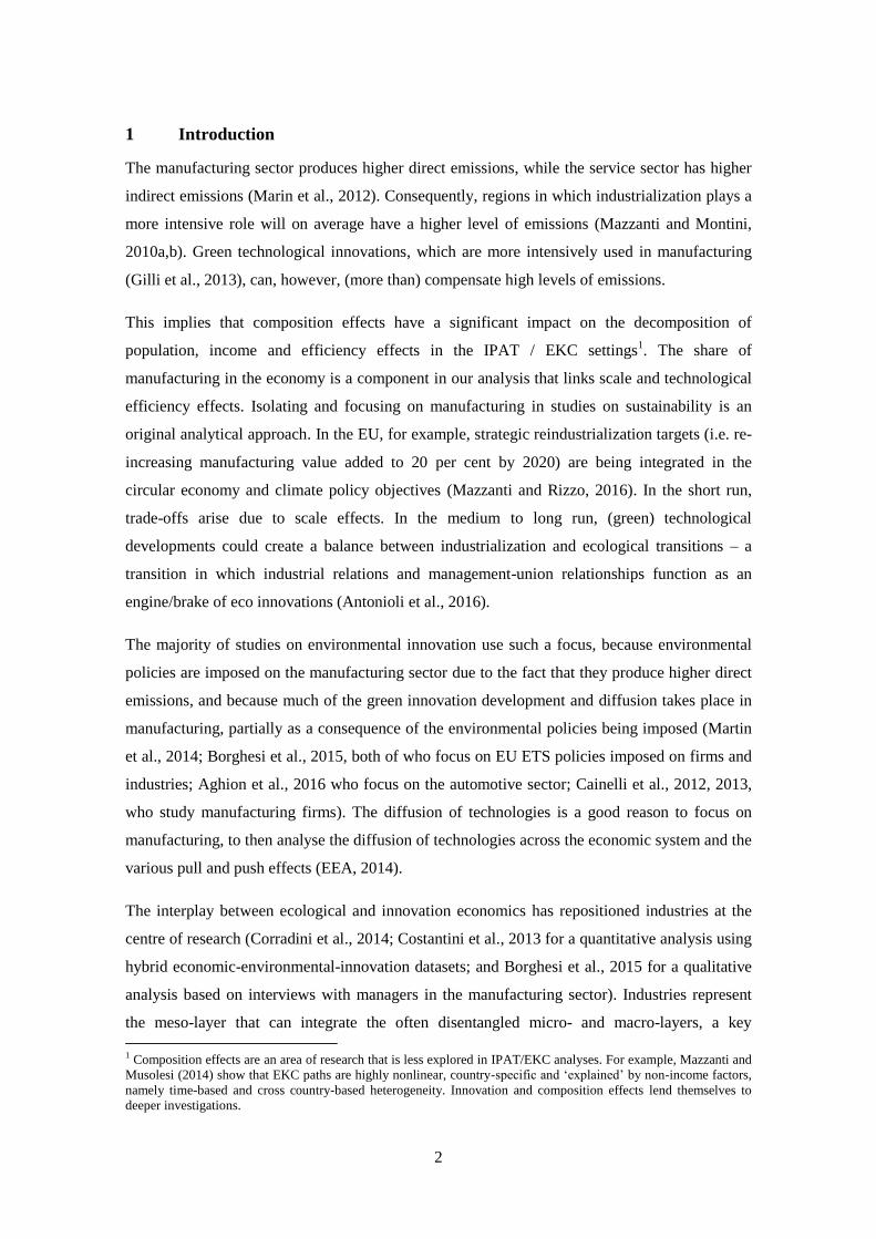
Figure 7 Fitted value (linear and quadratic) of manufacturing-related CO2 emissions
(consumption perspective) and GDP per capita (from fixed effect estimates
including year dummies) ......................................................................................... 16
Figure 8 Fitted value (linear and quadratic) of manufacturing-related material use
(consumption perspective) and GDP per capita (from fixed effect estimates
including year dummies) ......................................................................................... 16
Figure 9 Emissions per capita vs GDP per capita. CO2 in tons (production perspective) ..... 17
Figure 10 Emissions per capita vs GDP per capita. Co2 in tons (consumption perspective) ... 18
Figure 11 Emissions per capita vs GDP per capita. Material in 1,000 tons (indirect material
consumption) ........................................................................................................... 18
Figure 12 Sector-specific elasticity (linear) of CO2 emissions (production perspective) in
relation to GDP per capita (derived from fixed effect estimates including year
dummies) ................................................................................................................. 19
Figure 13 Fitted value (linear and quadratic) of final consumption of manufacturing goods
(value per capita) and GDP per capita (from fixed effect estimates including year
dummies) ................................................................................................................. 21
Figure 14 Sector-specific relationship between share of consumption by industry over total
consumption of manufacturing goods and the logarithm of GDP per capita (from
fixed effect estimates including year dummies) ...................................................... 23
Figure 15 Sector-specific elasticity (linear) of environmental pressure intensity in relation to
GDP per capita (from fixed effect estimates including year dummies) .................. 26

1
Abstract
This paper analyses the relationship between GDP and environmental impacts (e.g. CO2 and
indirect material use). It takes a manufacturing sector perspective at the global scale. The
analyses are based on a dynamics perspective. The level of sustainable development is
examined by looking at structural change and technology/efficiency components, as well as
scale-income effects. By carrying out a decomposition as well as a regression analysis, we first
find that industrialized countries are the only group that registered a negative trend for CO2
emissions over the study period. Second, of the three components included in our
decomposition analysis (scale, composition, efficiency), the scale effect always shows a positive
impact on total emissions, the exception being the group of least developed countries. Third, the
industry-by-industry analysis of income-CO2 elasticities reveals a strong monotonic relationship
between income and CO2 (from the production and consumption perspective) and indirect
material consumption. Finally, a detailed component-by-component analysis shows that (i) the
scale effect is relevant, as expected, (ii) the relationship between the composition effect and
GDP indicates a negative slope, i.e. the manufacturing sector becomes greener as income
increases, and (iii) technological change increases the environmental productivity of aggregate
manufacturing.
2
1 Introduction
The manufacturing sector produces higher direct emissions, while the service sector has higher
indirect emissions (Marin et al., 2012). Consequently, regions in which industrialization plays a
more intensive role will on average have a higher level of emissions (Mazzanti and Montini,
2010a,b). Green technological innovations, which are more intensively used in manufacturing
(Gilli et al., 2013), can, however, (more than) compensate high levels of emissions.
This implies that composition effects have a significant impact on the decomposition of
population, income and efficiency effects in the IPAT / EKC settings1. The share of
manufacturing in the economy is a component in our analysis that links scale and technological
efficiency effects. Isolating and focusing on manufacturing in studies on sustainability is an
original analytical approach. In the EU, for example, strategic reindustrialization targets (i.e. re-
increasing manufacturing value added to 20 per cent by 2020) are being integrated in the
circular economy and climate policy objectives (Mazzanti and Rizzo, 2016). In the short run,
trade-offs arise due to scale effects. In the medium to long run, (green) technological
developments could create a balance between industrialization and ecological transitions – a
transition in which industrial relations and management-union relationships function as an
engine/brake of eco innovations (Antonioli et al., 2016).
The majority of studies on environmental innovation use such a focus, because environmental
policies are imposed on the manufacturing sector due to the fact that they produce higher direct
emissions, and because much of the green innovation development and diffusion takes place in
manufacturing, partially as a consequence of the environmental policies being imposed (Martin
et al., 2014; Borghesi et al., 2015, both of who focus on EU ETS policies imposed on firms and
industries; Aghion et al., 2016 who focus on the automotive sector; Cainelli et al., 2012, 2013,
who study manufacturing firms). The diffusion of technologies is a good reason to focus on
manufacturing, to then analyse the diffusion of technologies across the economic system and the
various pull and push effects (EEA, 2014).
The interplay between ecological and innovation economics has repositioned industries at the
centre of research (Corradini et al., 2014; Costantini et al., 2013 for a quantitative analysis using
hybrid economic-environmental-innovation datasets; and Borghesi et al., 2015 for a qualitative
analysis based on interviews with managers in the manufacturing sector). Industries represent
the meso-layer that can integrate the often disentangled micro- and macro-layers, a key
1 Composition effects are an area of research that is less explored in IPAT/EKC analyses. For example, Mazzanti and
Musolesi (2014) show that EKC paths are highly nonlinear, country-specific and ‘explained’ by non-income factors,
namely time-based and cross country-based heterogeneity. Innovation and composition effects lend themselves to
deeper investigations.
3
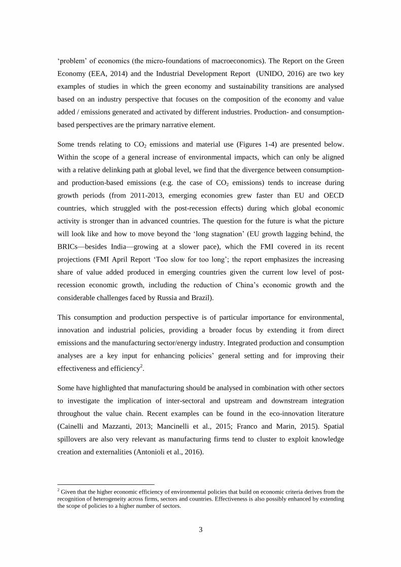
‘problem’ of economics (the micro-foundations of macroeconomics). The Report on the Green
Economy (EEA, 2014) and the Industrial Development Report (UNIDO, 2016) are two key
examples of studies in which the green economy and sustainability transitions are analysed
based on an industry perspective that focuses on the composition of the economy and value
added / emissions generated and activated by different industries. Production- and consumption-
based perspectives are the primary narrative element.
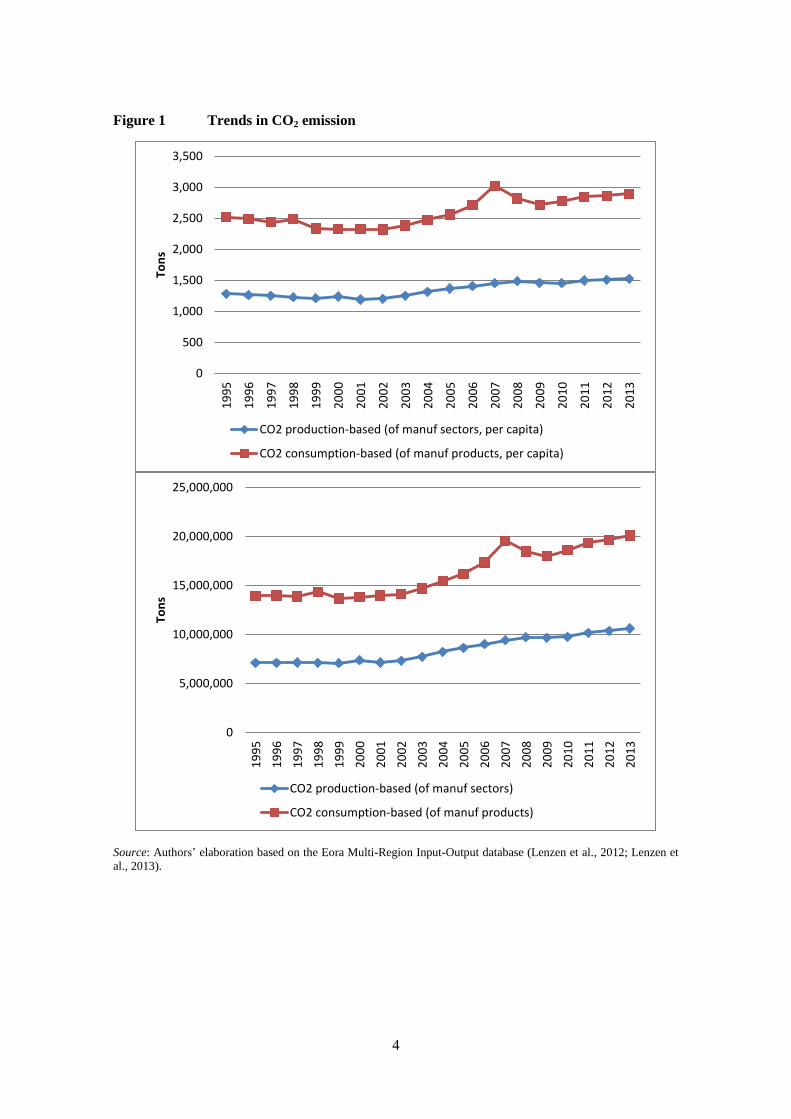
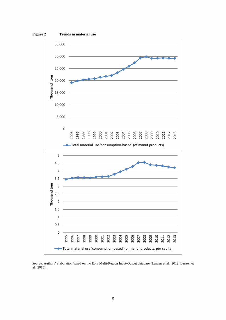
Some trends relating to CO2 emissions and material use (Figures 1-4) are presented below.
Within the scope of a general increase of environmental impacts, which can only be aligned
with a relative delinking path at global level, we find that the divergence between consumption-
and production-based emissions (e.g. the case of CO2 emissions) tends to increase during
growth periods (from 2011-2013, emerging economies grew faster than EU and OECD
countries, which struggled with the post-recession effects) during which global economic
activity is stronger than in advanced countries. The question for the future is what the picture
will look like and how to move beyond the ‘long stagnation’ (EU growth lagging behind, the
BRICs—besides India—growing at a slower pace), which the FMI covered in its recent
projections (FMI April Report ‘Too slow for too long’; the report emphasizes the increasing
share of value added produced in emerging countries given the current low level of post-
recession economic growth, including the reduction of China’s economic growth and the
considerable challenges faced by Russia and Brazil).
This consumption and production perspective is of particular importance for environmental,
innovation and industrial policies, providing a broader focus by extending it from direct
emissions and the manufacturing sector/energy industry. Integrated production and consumption
analyses are a key input for enhancing policies’ general setting and for improving their
effectiveness and efficiency2.
Some have highlighted that manufacturing should be analysed in combination with other sectors
to investigate the implication of inter-sectoral and upstream and downstream integration
throughout the value chain. Recent examples can be found in the eco-innovation literature
(Cainelli and Mazzanti, 2013; Mancinelli et al., 2015; Franco and Marin, 2015). Spatial
spillovers are also very relevant as manufacturing firms tend to cluster to exploit knowledge
creation and externalities (Antonioli et al., 2016).
2 Given that the higher economic efficiency of environmental policies that build on economic criteria derives from the
recognition of heterogeneity across firms, sectors and countries. Effectiveness is also possibly enhanced by extending
the scope of policies to a higher number of sectors.
4
Figure 1 Trends in CO2 emission
Source: Authors’ elaboration based on the Eora Multi-Region Input-Output database (Lenzen et al., 2012; Lenzen et
al., 2013).
0
500
1,000
1,500
2,000
2,500
3,000
3,500
19
95
19
96
19
97
19
98
19
99
20
00
20
01
20
02
20
03
20
04
20
05
20
06
20
07
20
08
20
09
20
10
20
11
20
12
20
13
Ton
s
CO2 production-based (of manuf sectors, per capita)
CO2 consumption-based (of manuf products, per capita)
0
5,000,000
10,000,000
15,000,000
20,000,000
25,000,000
19
95
19
96
19
97
19
98
19
99
20
00
20
01
20
02
20
03
20
04
20
05
20
06
20
07
20
08
20
09
20
10
20
11
20
12
20
13
Ton
s
CO2 production-based (of manuf sectors)
CO2 consumption-based (of manuf products)
5
Figure 2 Trends in material use
Source: Authors’ elaboration based on the Eora Multi-Region Input-Output database (Lenzen et al., 2012; Lenzen et
al., 2013).
0
5,000
10,000
15,000
20,000
25,000
30,000
35,000
19
95
19
96
19
97
19
98
19
99
20
00
20
01
20
02
20
03
20
04
20
05
20
06
20
07
20
08
20
09
20
10
20
11
20
12
20
13
Tho
usa
nd
to
ns
Total material use 'consumption-based' (of manuf products)
0
0.5
1
1.5
2
2.5
3
3.5
4
4.5
5
19
95
19
96
19
97
19
98
19
99
20
00
20
01
20
02
20
03
20
04
20
05
20
06
20
07
20
08
20
09
20
10
20
11
20
12
20
13
Tho
usa
nd
to
ns
Total material use 'consumption-based' (of manuf products, per capita)
6
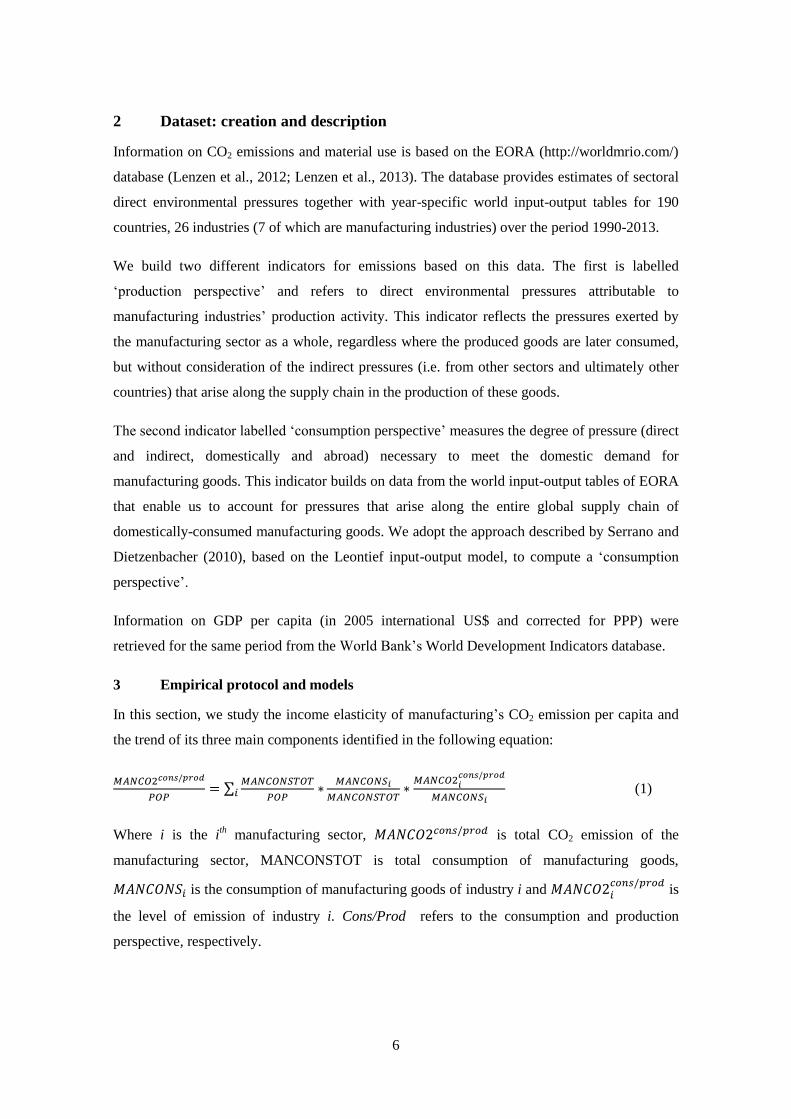
2 Dataset: creation and description
Information on CO2 emissions and material use is based on the EORA (http://worldmrio.com/)
database (Lenzen et al., 2012; Lenzen et al., 2013). The database provides estimates of sectoral
direct environmental pressures together with year-specific world input-output tables for 190
countries, 26 industries (7 of which are manufacturing industries) over the period 1990-2013.
We build two different indicators for emissions based on this data. The first is labelled
‘production perspective’ and refers to direct environmental pressures attributable to
manufacturing industries’ production activity. This indicator reflects the pressures exerted by
the manufacturing sector as a whole, regardless where the produced goods are later consumed,
but without consideration of the indirect pressures (i.e. from other sectors and ultimately other
countries) that arise along the supply chain in the production of these goods.
The second indicator labelled ‘consumption perspective’ measures the degree of pressure (direct
and indirect, domestically and abroad) necessary to meet the domestic demand for
manufacturing goods. This indicator builds on data from the world input-output tables of EORA
that enable us to account for pressures that arise along the entire global supply chain of
domestically-consumed manufacturing goods. We adopt the approach described by Serrano and
Dietzenbacher (2010), based on the Leontief input-output model, to compute a ‘consumption
perspective’.
Information on GDP per capita (in 2005 international US$ and corrected for PPP) were
retrieved for the same period from the World Bank’s World Development Indicators database.
3 Empirical protocol and models
In this section, we study the income elasticity of manufacturing’s CO2 emission per capita and
the trend of its three main components identified in the following equation:
𝑀𝐴𝑁𝐶𝑂2𝑐𝑜𝑛𝑠/𝑝𝑟𝑜𝑑
𝑃𝑂𝑃= ∑
𝑀𝐴𝑁𝐶𝑂𝑁𝑆𝑇𝑂𝑇
𝑃𝑂𝑃∗𝑖
𝑀𝐴𝑁𝐶𝑂𝑁𝑆𝑖
𝑀𝐴𝑁𝐶𝑂𝑁𝑆𝑇𝑂𝑇∗
𝑀𝐴𝑁𝐶𝑂2𝑖𝑐𝑜𝑛𝑠/𝑝𝑟𝑜𝑑
𝑀𝐴𝑁𝐶𝑂𝑁𝑆𝑖 (1)
Where i is the ith manufacturing sector, 𝑀𝐴𝑁𝐶𝑂2𝑐𝑜𝑛𝑠/𝑝𝑟𝑜𝑑 is total CO2 emission of the
manufacturing sector, MANCONSTOT is total consumption of manufacturing goods,
𝑀𝐴𝑁𝐶𝑂𝑁𝑆𝑖 is the consumption of manufacturing goods of industry i and 𝑀𝐴𝑁𝐶𝑂2𝑖𝑐𝑜𝑛𝑠/𝑝𝑟𝑜𝑑
is
the level of emission of industry i. Cons/Prod refers to the consumption and production
perspective, respectively.
7
The right hand side of the equation presents a simple decomposition of total CO2 per capita,
where (i) the first term is the scale or wealth effect, i.e. the effect of the manufacturing sector’s
size per capita; (ii) the second term is a composition effect, i.e. the effect of a change in the
impact of the growth of one industry with respect to others; (iii) while the third term is a
technical effect, i.e. the sum of environmental impacts of every single industry measured as the
ratio between sectoral CO2 emission and sectoral consumption of manufacturing goods. We
therefore apply the following set of equations:
𝑀𝐴𝑁𝐶𝑂2𝑐𝑜𝑛𝑠/𝑝𝑟𝑜𝑑
𝑃𝑂𝑃= 𝛼𝑖 + 𝜏𝑡+𝛽1𝐺𝐷𝑃𝑝𝑐𝑖𝑡 + 𝜀𝑖𝑡 (2)
𝑀𝐴𝑁𝐶𝑂𝑁𝑆𝑇𝑂𝑇
𝑃𝑂𝑃= 𝛼𝑖 + 𝜏𝑡+𝛽1𝐺𝐷𝑃𝑝𝑐𝑖𝑡 + 𝜀𝑖𝑡 (3)
𝑀𝐴𝑁𝐶𝑂𝑁𝑆𝑖
𝑀𝐴𝑁𝐶𝑂𝑁𝑆𝑇𝑂𝑇= 𝛼𝑖 + 𝜏𝑡+𝛽1𝐺𝐷𝑃𝑝𝑐𝑖𝑡 + 𝜀𝑖𝑡 (4)
𝑀𝐴𝑁𝐶𝑂𝑖𝑐𝑜𝑛𝑠/𝑝𝑟𝑜𝑑
𝑀𝐴𝑁𝐶𝑂𝑁𝑆𝑖= 𝛼𝑖 + 𝜏𝑡+𝛽1𝐺𝐷𝑃𝑝𝑐𝑖𝑡 + 𝜀𝑖𝑡 (5)
Where 𝛼𝑡 is a fixed effect varying across countries, 𝜏𝑡 is the year fixed effect, and 𝜀𝑖𝑡 is a
stochastic error term. All estimations present cluster robust standard errors and are run with
ordinary least squared estimators. All variables are log transformed.
Equations 2-5 test the environmental Kuznets hypothesis (Mazzanti et al., 2010). We adopt a
cubic form as a first reference (now illustrated in 2-5 for the sake of brevity). Whether a cubic,
quadratic or linear form is coherent with the available data is an empirical issue that we will
address on a case-by-case basis3. The quadratic form is associated with absolute delinking and
the linear form might present a case of relative delinking if the elasticities are significantly
lower than 1.
The analysis is structured as follows: using a decomposition analysis, Section 4 presents
descriptive evidence of the trend of the above mentioned components across different income
groups over the period 1995-2013. Section 5 presents the result of the empirical analysis
according to the specifications of Equations 2 to 5. The decomposition analysis and the
econometric analyses will elucidate different results: the two analyses complement each other
3 We adopt the typical general to specific reduction approach introduced by the LSE School of Econometrics
(Hendry, 1980): the final econometric specification derives not only from economic theory, but also from a fit with
the available data. “The theory of reduction explains how econometric models are intrinsically a kind of empirical
model, derived from the data-generating process (DGP). The general-to-specific approach mimics the theory of
reduction, and directs econometricians to obtain the final econometric model. The theory of reduction and the
general-to-specific approach demonstrate the fact that the LSE approach is an empiricist methodology in which
econometric models are said to match the phenomena in all measurable respects” (Chao, 2002).

8
and are consequential in logic. We account for the manufacturing industries’ environmental
impact based on three different perspectives: the production perspective (emission of CO2),
consumption perspective (emission of CO2) and indirect material consumption. Both the
decomposition and the econometric analysis capture interesting factors that are of relevance for
environmental policy and circular economy strategies. Finally, section 6 concludes.
4 Decomposition analysis
We decompose the manufacturing sector’s per capita environmental pressures (either direct or
‘consumption-based’) into various components as described in Equation 2:
Scale component => level of value added per capita (for direct pressures) or final
demand of domestic consumers per capita (for ‘consumption-based’ pressures)
𝑀𝐴𝑁𝐶𝑂𝑁𝑆𝑇𝑂𝑇
𝑃𝑂𝑃
Composition component => share of production or consumption of a specific
manufacturing industry over total production or consumption 𝑀𝐴𝑁𝐶𝑂𝑁𝑆𝑖
𝑀𝐴𝑁𝐶𝑂𝑁𝑆𝑇𝑂𝑇
Intensity component => environmental pressures per unit of production or consumption
𝑀𝐴𝑁𝐶𝑂2𝑖𝑐𝑜𝑛𝑠/𝑝𝑟𝑜𝑑
𝑀𝐴𝑁𝐶𝑂𝑁𝑆𝑖
The results are presented for four different country groups (according to UNIDO’s definition).
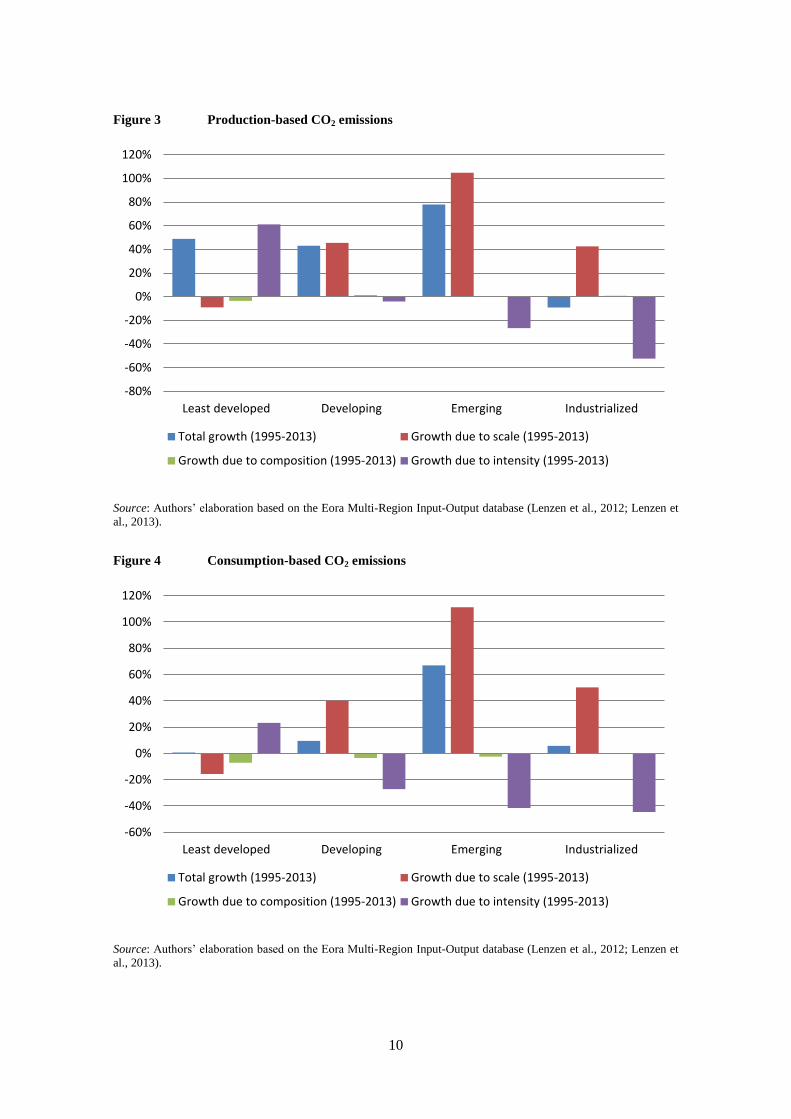
Adopting a production perspective, Figure 3 highlights a striking difference across the four
different income groups. Firstly, we note that “industrialized” countries is the only group
associated with a negative trend for CO2 emissions in the period analysed (1995-2013), while
the other three groups registered a significant increase in emissions.
Among the three components, the wealth effect has a positive impact on total emissions in each
case, with the exception of the “least developed countries” group, where it is negative.
The composition effect, by contrast, has a similar and negligible impact on the four income
groups, while the technical effect indicates some important heterogeneity. Technical
improvements have reduced total emissions in all income groups, with the exception of “least
developed countries”, in which the emission associated with this effect increased over the period
analysed.
The picture that emerges is particularly interesting. It highlights the very critical economic and
environmental situation in least developed countries, which have witnessed economic stagnation
even during a fairly positive period of growth among developing and emerging countries despite
9
the 2008-2009 downturn. Developing countries were able to jump on the growth train, but did
not exploit the period of growth to sustain efficient economic activities. As the composition of
economic activities in developing countries remained negligible, the compensation effect of
efficiency factors was only marginal. In the post-Kyoto phase, notwithstanding the diffusion of
CDM projects worldwide4, LDCs and developing countries neither exploited policy-induced
effects nor technological diffusion. The new Green Climate Fund (GCF) should take this
finding into consideration when financing mitigation and adaptation projects5.
The (expected) growth-led emissions path of emerging countries with some signs of
compensation indicates that internal innovation mechanisms and international transfers of
technology have had an impact on the overall trend of emissions.
Due to the more stable composition of the economy in industrialized countries, they
successfully compensated scale effects with higher efficiency.
These findings do not change significantly when we adopt a consumption perspective, as
illustrated in Figure 4. A comparison between the two perspectives reveals that: (i) exports from
LDCs and developing countries are quite inefficient in environmental terms; (ii) this
inefficiency is also present in emerging countries but to a lower degree; (iii) this is reflected in
the minor role the third component plays in wealthier countries (Figure 6). The difference is not
particularly large due to the still relevant role intra-regional trade (e.g. intra-EU) plays.
Nevertheless, the increasing share of trade between richer and poorer areas gives these findings
considerable significance. They provide a clear message in favour of sustaining deeper
international green techno-organizational diffusion of management practices.
4 For overviews of the distribution of projects by host parties, regional areas and destinations of CDM investments,
we refer to Costantini and Sforna (2014). As far as host parties are concerned, China, Brazil and India represent
around 73 per cent of the total, with China attributing for 48 per cent. Asia and the Pacific amount to more than 80
per cent, with Africa and the MENA Region lagging behind with a total amount of only 3 per cent. Finally, looking at
monetary efforts (investments), China and India represent about 85 per cent in total (China contributes 65 per cent).
The overall distribution is quite biased and linked to strong trade players. This shows that CDM complements
existing projects and reinforces current trade dynamics. CDM investments add value to existing trade/investment
relationships. China and India rank only 6th and 8th in terms of efficiency (saved CO2 / millions US$ invested), with
the Republic of Korea, Brazil and Argentina taking the first three positions. 5 http://www.siecon.org/online/wp-content/uploads/2016/09/COSTANTINI.pdf (paper presented by Anil Markandya
at the last Italian Economic Association conference held at the Bocconi University, Milan, October 2016, during the
IAERE session.
10
Figure 3 Production-based CO2 emissions
Source: Authors’ elaboration based on the Eora Multi-Region Input-Output database (Lenzen et al., 2012; Lenzen et
al., 2013).
Figure 4 Consumption-based CO2 emissions
Source: Authors’ elaboration based on the Eora Multi-Region Input-Output database (Lenzen et al., 2012; Lenzen et
al., 2013).
-80%
-60%
-40%
-20%
0%
20%
40%
60%
80%
100%
120%
Least developed Developing Emerging Industrialized
Total growth (1995-2013) Growth due to scale (1995-2013)
Growth due to composition (1995-2013) Growth due to intensity (1995-2013)
-60%
-40%
-20%
0%
20%
40%
60%
80%
100%
120%
Least developed Developing Emerging Industrialized
Total growth (1995-2013) Growth due to scale (1995-2013)
Growth due to composition (1995-2013) Growth due to intensity (1995-2013)
11
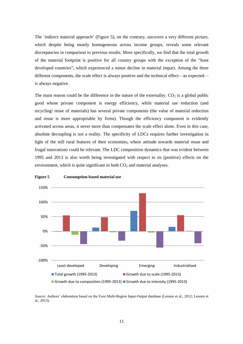
The ‘indirect material approach’ (Figure 5), on the contrary, uncovers a very different picture,
which despite being mostly homogeneous across income groups, reveals some relevant
discrepancies in comparison to previous results. More specifically, we find that the total growth
of the material footprint is positive for all country groups with the exception of the “least
developed countries”, which experienced a minor decline in material impact. Among the three
different components, the scale effect is always positive and the technical effect—as expected—
is always negative.
The main reason could be the difference in the nature of the externality. CO2 is a global public
good whose private component is energy efficiency, while material use reduction (and
recycling/ reuse of materials) has several private components (the value of material reduction
and reuse is more appropriable by firms). Though the efficiency component is evidently
activated across areas, it never more than compensates the scale effect alone. Even in this case,
absolute decoupling is not a reality. The specificity of LDCs requires further investigation in
light of the still rural features of their economies, where attitude towards material reuse and
frugal innovations could be relevant. The LDC composition dynamics that was evident between
1995 and 2013 is also worth being investigated with respect to its (positive) effects on the
environment, which is quite significant in both CO2 and material analyses.
Figure 5 Consumption-based material use
Source: Authors’ elaboration based on the Eora Multi-Region Input-Output database (Lenzen et al., 2012; Lenzen et
al., 2013).
-100%
-50%
0%
50%
100%
150%
Least developed Developing Emerging Industrialized
Total growth (1995-2013) Growth due to scale (1995-2013)
Growth due to composition (1995-2013) Growth due to intensity (1995-2013)
12
5 Econometric analysis
5.1 Total emissions
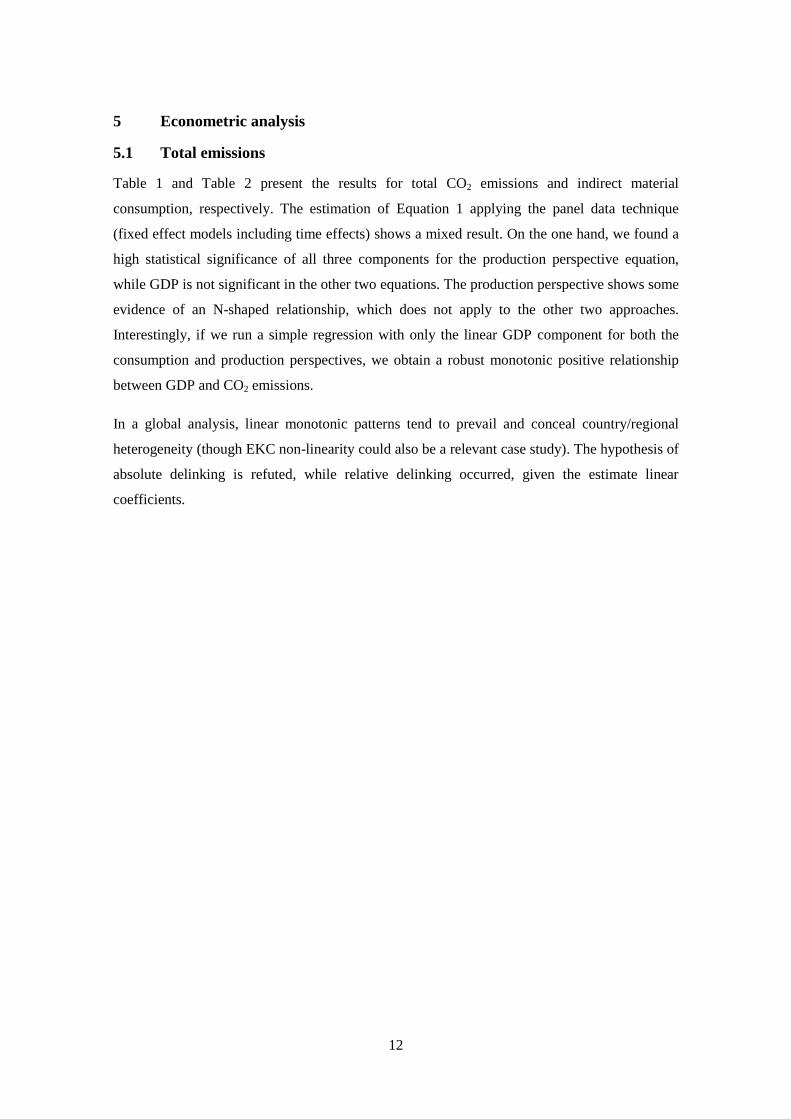
Table 1 and Table 2 present the results for total CO2 emissions and indirect material
consumption, respectively. The estimation of Equation 1 applying the panel data technique
(fixed effect models including time effects) shows a mixed result. On the one hand, we found a
high statistical significance of all three components for the production perspective equation,
while GDP is not significant in the other two equations. The production perspective shows some
evidence of an N-shaped relationship, which does not apply to the other two approaches.
Interestingly, if we run a simple regression with only the linear GDP component for both the
consumption and production perspectives, we obtain a robust monotonic positive relationship
between GDP and CO2 emissions.
In a global analysis, linear monotonic patterns tend to prevail and conceal country/regional
heterogeneity (though EKC non-linearity could also be a relevant case study). The hypothesis of
absolute delinking is refuted, while relative delinking occurred, given the estimate linear
coefficients.
13
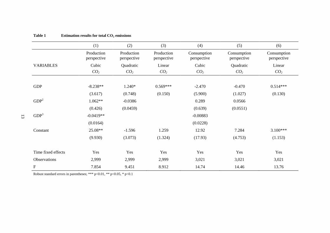
Table 1 Estimation results for total CO2 emissions
(1) (2) (3) (4) (5) (6)
Production
perspective
Production
perspective
Production
perspective
Consumption
perspective
Consumption
perspective
Consumption
perspective
VARIABLES Cubic
CO2
Quadratic
CO2
Linear
CO2
Cubic
CO2
Quadratic
CO2
Linear
CO2
GDP -8.238** 1.240* 0.569*** -2.470 -0.470 0.514***
(3.617) (0.748) (0.150) (5.900) (1.027) (0.130)
GDP2 1.062** -0.0386 0.289 0.0566
(0.426) (0.0459) (0.639) (0.0551)
GDP3 -0.0419** -0.00883
(0.0164) (0.0228)
Constant 25.08** -1.596 1.259 12.92 7.284 3.100***
(9.930) (3.073) (1.324) (17.93) (4.753) (1.153)
Time fixed effects Yes Yes Yes Yes Yes Yes
Observations 2,999 2,999 2,999 3,021 3,021 3,021
F 7.854 9.451 8.912 14.74 14.46 13.76
Robust standard errors in parentheses; *** p<0.01, ** p<0.05, * p<0.1

14
Table 2 Estimation results for total (indirect) material consumption
(1)
Consumption Perspective
(2)
Consumption Perspective
(3)
Consumption Perspective
VARIABLES Cubic
Material consuption
Quadratic
Material consumption
Linear
Material consumption
GDP -2.244 0.0865 0.674***
(1.999) (0.486) (0.0852)
GDP2 0.304 0.0338
(0.232) (0.0260)
GDP3 -0.0103
(0.00879)
Constant 4.051 -2.508 -5.007***
(5.671) (2.285) (0.753)
Time fixed effects Yes Yes Yes
Observations 3,021 3,021 3,021
F 28.69 28.42 25.55
Robust standard errors in parentheses; *** p<0.01, ** p<0.05, * p<0.1
15
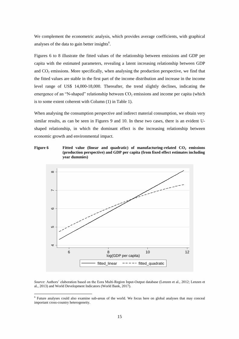
We complement the econometric analysis, which provides average coefficients, with graphical
analyses of the data to gain better insights6.
Figures 6 to 8 illustrate the fitted values of the relationship between emissions and GDP per
capita with the estimated parameters, revealing a latent increasing relationship between GDP
and CO2 emissions. More specifically, when analysing the production perspective, we find that
the fitted values are stable in the first part of the income distribution and increase in the income
level range of US$ 14,000-18,000. Thereafter, the trend slightly declines, indicating the
emergence of an “N-shaped” relationship between CO2 emissions and income per capita (which
is to some extent coherent with Column (1) in Table 1).
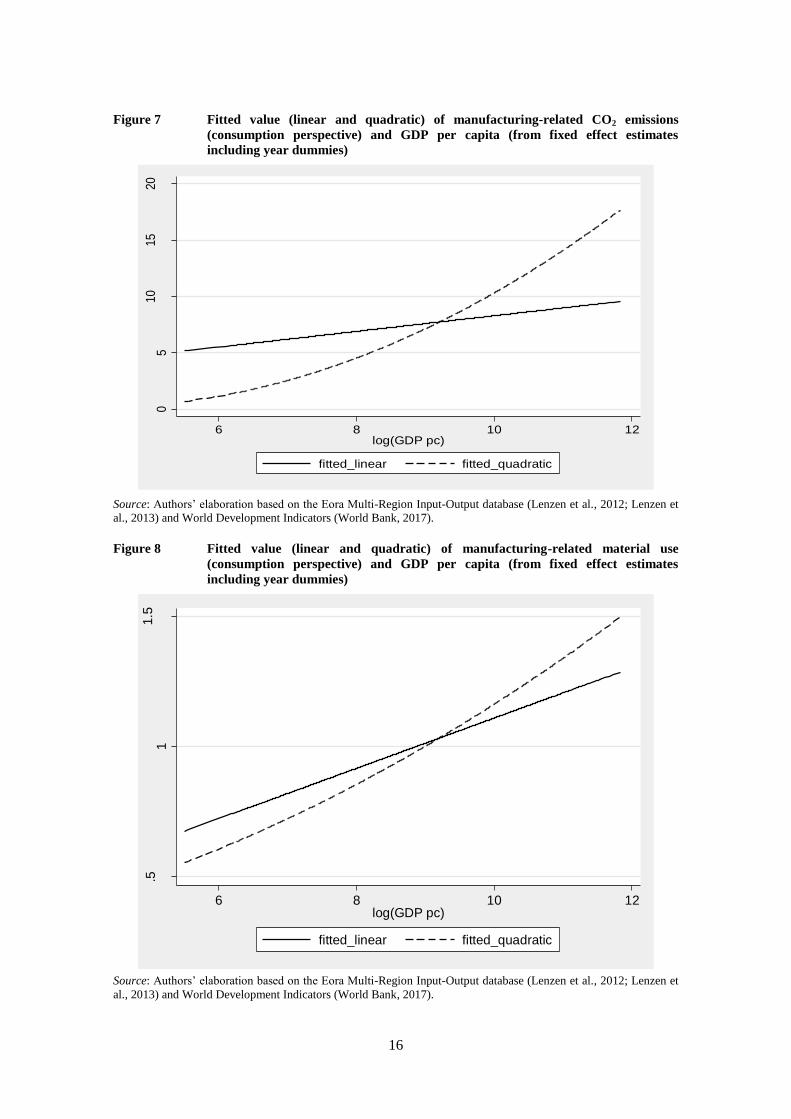
When analysing the consumption perspective and indirect material consumption, we obtain very
similar results, as can be seen in Figures 9 and 10. In these two cases, there is an evident U-
shaped relationship, in which the dominant effect is the increasing relationship between
economic growth and environmental impact.
Figure 6 Fitted value (linear and quadratic) of manufacturing-related CO2 emissions
(production perspective) and GDP per capita (from fixed effect estimates including
year dummies)
Source: Authors’ elaboration based on the Eora Multi-Region Input-Output database (Lenzen et al., 2012; Lenzen et
al., 2013) and World Development Indicators (World Bank, 2017).
6 Future analyses could also examine sub-areas of the world. We focus here on global analyses that may conceal
important cross-country heterogeneity.
45
67
8
6 8 10 12log(GDP per capita)
fitted_linear fitted_quadratic
16
Figure 7 Fitted value (linear and quadratic) of manufacturing-related CO2 emissions
(consumption perspective) and GDP per capita (from fixed effect estimates
including year dummies)
Source: Authors’ elaboration based on the Eora Multi-Region Input-Output database (Lenzen et al., 2012; Lenzen et
al., 2013) and World Development Indicators (World Bank, 2017).
Figure 8 Fitted value (linear and quadratic) of manufacturing-related material use
(consumption perspective) and GDP per capita (from fixed effect estimates
including year dummies)
Source: Authors’ elaboration based on the Eora Multi-Region Input-Output database (Lenzen et al., 2012; Lenzen et
al., 2013) and World Development Indicators (World Bank, 2017).
05
10
15
20
6 8 10 12log(GDP pc)
fitted_linear fitted_quadratic
.51
1.5
6 8 10 12log(GDP pc)
fitted_linear fitted_quadratic

17
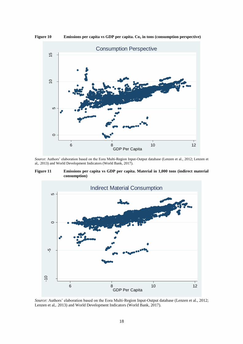
This trend is also confirmed by the three scatter plots presented in Figures 9-11, where each dot
represents the combination of each emissions/CO2 pair in the analysed period for each country.
The trend of the three aggregates is slightly different: the production perspective shows some
non-linearity in the lower tail of income distribution, while the main part of the distribution
confirms a strong increasing relationship between GDP and CO2 per capita. Similarly, in
correspondence to the upper part of income distribution, we see some variability in CO2 per
capita, with several observations below the mean. This tendency might be reflected in the N-
shape trend registered in the estimations (Column 1). By contrast, the scatter plot for both the
consumption and indirect material consumption perspectives indicate an increasing relationship,
confirming the regression results. Overall, against the fitted values and plots evidence, which
reveal some heterogeneity, the econometric analysis seems to convey that a linear relationship
describes the CO2-GDP trends globally.
Figure 9 Emissions per capita vs GDP per capita. CO2 in tons (production perspective)
Source: Authors’ elaboration based on the Eora Multi-Region Input-Output database (Lenzen et al., 2012;
Lenzen et al., 2013) and World Development Indicators (World Bank, 2017).
02
46
810
Co2 P
er
Capita
6 8 10 12GDP Per Capita
Production Perspective
18
Figure 10 Emissions per capita vs GDP per capita. Co2 in tons (consumption perspective)
Source: Authors’ elaboration based on the Eora Multi-Region Input-Output database (Lenzen et al., 2012; Lenzen et
al,. 2013) and World Development Indicators (World Bank, 2017).
Figure 11 Emissions per capita vs GDP per capita. Material in 1,000 tons (indirect material
consumption)
Source: Authors’ elaboration based on the Eora Multi-Region Input-Output database (Lenzen et al., 2012;
Lenzen et al,. 2013) and World Development Indicators (World Bank, 2017).
05
10
15
Co2 P
er
Capita
6 8 10 12GDP Per Capita
Consumption Perspective-1
0-5
05
Mate
rial P
er
Capita
6 8 10 12GDP Per Capita
Indirect Material Consumption

19
5.2 Elasticity of emissions (in relation to GDP)
Figure 12 illustrates the elasticity of emissions of each manufacturing industry according to the
production, consumption and indirect material perspective. In this specific case, we estimated
the following regression to derive direct elasticity. All variables are log transformed:
𝑀𝐴𝑁𝐶𝑂2𝑐𝑜𝑛𝑠/𝑝𝑟𝑜𝑑
𝑃𝑂𝑃= 𝛼𝑖𝑡+𝛽1𝐺𝐷𝑃𝑖𝑡 + 𝜀𝑖𝑡
(6)
Figure 12 Sector-specific elasticity (linear) of CO2 emissions (production perspective) in
relation to GDP per capita (derived from fixed effect estimates including year
dummies)
Source: Authors’ elaboration based on the Eora Multi-Region Input-Output database (Lenzen et al., 2012; Lenzen et
al., 2013) and World Development Indicators (World Bank, 2017).
0 .2 .4 .6 .8
Wood and Paper
Transport Equipment
Textiles and Wearing Apparel
Recycling
Petroleum, Chemical and Non-Metallic Mineral Products
Other Manufacturing
Metal Products
Food & Beverages
Electrical and Machinery
Elasticity between CO2 pc (prod perspective) and GDP pc
Elasticity between CO2 pc (cons perspective) and GDP pc
Elasticity between material use pc (cons perspective) and GDP pc

20
The estimations of simple elasticities confirm the previous findings of a strong monotonic
relationship between income and CO2 production, shown in the aforementioned graphical
analysis as well as in the regressions (Table 1). This is much more pronounced for the
consumption and indirect material consumption perspectives, where the elasticity is always
statistically significant and associated with a positive coefficient. The production perspective,
by contrast, shows that four industries do not have a significant linear effect, a result that
possibly drives the N-shape effect presented in Column 1of Table 1, and is generally a less
clear-cut outcome as far as the findings on the production perspective are concerned.
5.3 Wealth effect
Table 3 presents the results for the wealth component of total CO2 emissions, reflecting the
scale of the manufacturing sector (see Equation 3). Figure 13 plots the fitted value (linear and
quadratic) of the relationship between the final consumption of manufacturing goods and GDP
per capita.
Table 3 Estimation results for the wealth effect
(1)
VARIABLES Wealth effect
GDP -7.588***
(2.491)
GDP2 1.030***
(0.290)
GDP3 -0.0400***
(0.0111)
Constant 27.37***
(7.172)
Time fixed effects Yes
Observations 3,021
F 170.4
Robust standard errors in parentheses
*** p<0.01, ** p<0.05, * p<0.1

21
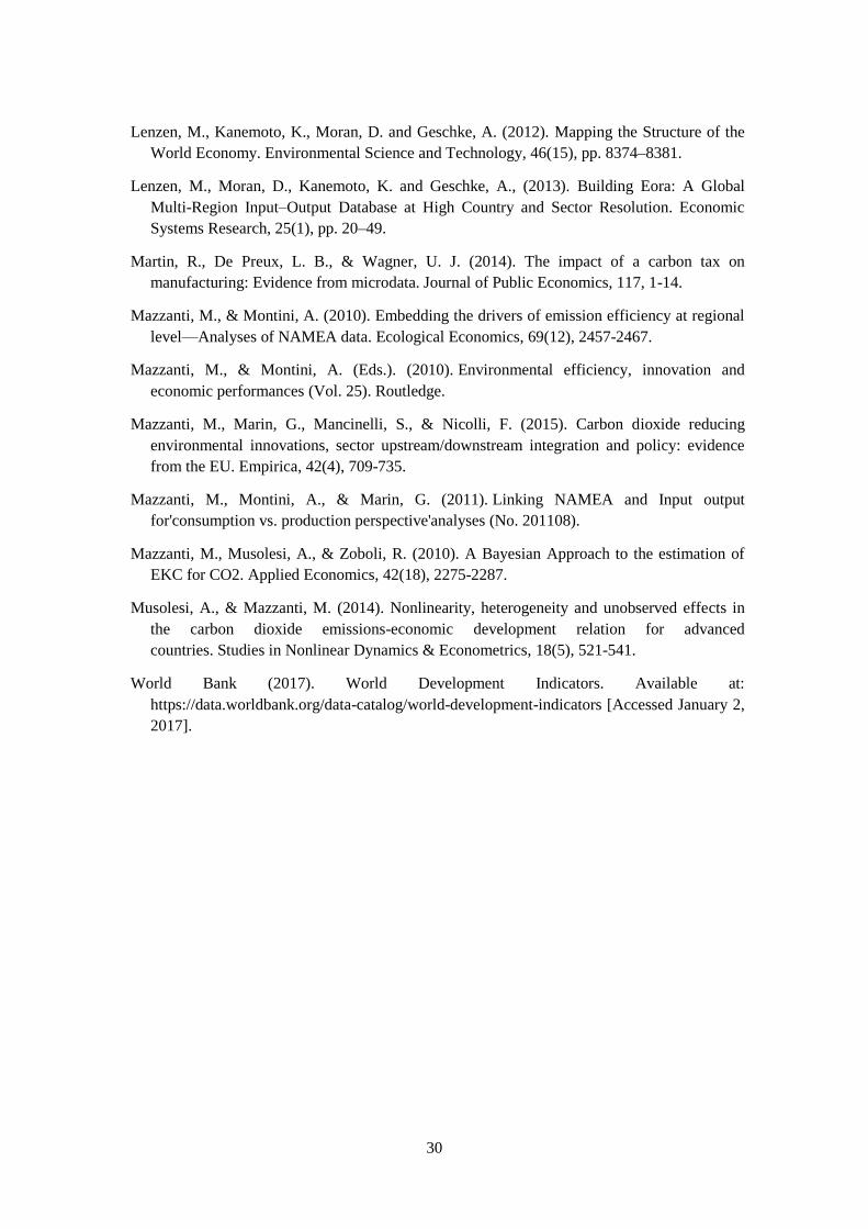
The regression results as well as Figure A1 in the Appendix show that the total consumption of
manufacturing goods per capita increases with income, though this occurs at a different speed.
In the lower part of the distribution of income per capita, the growth of the manufacturing sector
is still slow while the elasticity increases in intensity when income rises.
Figure 13 Fitted value (linear and quadratic) of final consumption of manufacturing goods
(value per capita) and GDP per capita (from fixed effect estimates including year
dummies)
Source: Authors’ elaboration based on the Eora Multi-Region Input-Output database (Lenzen et al., 2012; Lenzen et
al., 2013) and World Development Indicators (World Bank, 2017).
5.4 Composition effect
Table 4 presents the results for the aggregate composition component of total CO2 emissions,
reflecting the effect of a change in the impact of the growth of one industry in comparison to the
others (see Equation 4). The overall trend is analysed with more compelling details by industry
in Figure 14, demonstrating significant differences across industries.
810
12
14
16
18
6 8 10 12log(GDP pc)
fitted_linear fitted_quadratic
22
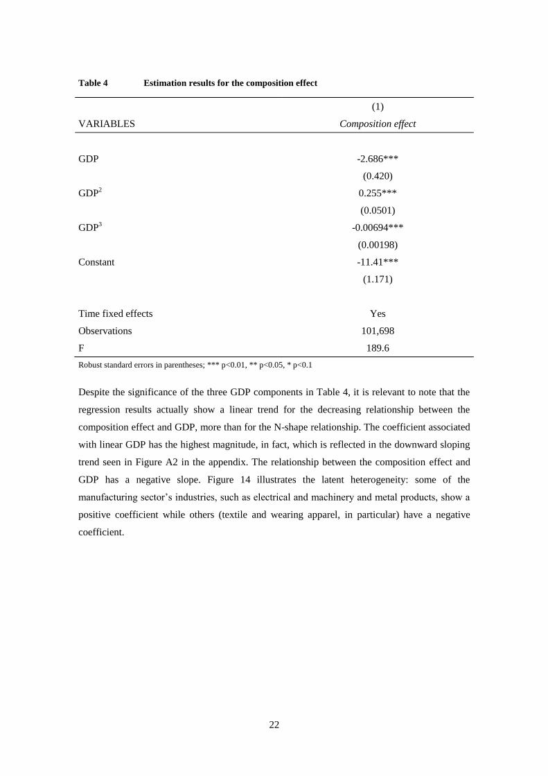
Table 4 Estimation results for the composition effect
(1)
VARIABLES Composition effect
GDP -2.686***
(0.420)
GDP2 0.255***
(0.0501)
GDP3 -0.00694***
(0.00198)
Constant -11.41***
(1.171)
Time fixed effects Yes
Observations 101,698
F 189.6
Robust standard errors in parentheses; *** p<0.01, ** p<0.05, * p<0.1
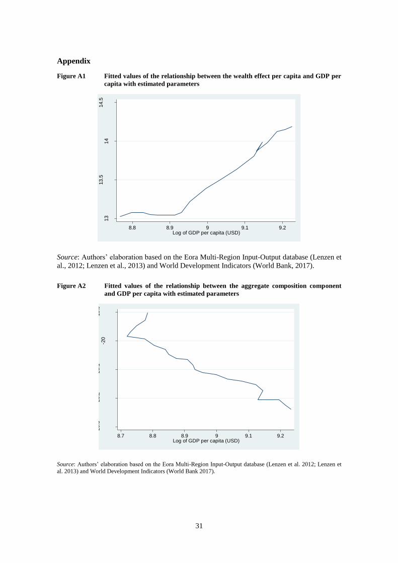
Despite the significance of the three GDP components in Table 4, it is relevant to note that the
regression results actually show a linear trend for the decreasing relationship between the
composition effect and GDP, more than for the N-shape relationship. The coefficient associated
with linear GDP has the highest magnitude, in fact, which is reflected in the downward sloping
trend seen in Figure A2 in the appendix. The relationship between the composition effect and
GDP has a negative slope. Figure 14 illustrates the latent heterogeneity: some of the
manufacturing sector’s industries, such as electrical and machinery and metal products, show a
positive coefficient while others (textile and wearing apparel, in particular) have a negative
coefficient.

23
Figure 14 Sector-specific relationship between share of consumption by industry over total
consumption of manufacturing goods and the logarithm of GDP per capita (from
fixed effect estimates including year dummies)
Source: Authors’ elaboration based on the Eora Multi-Region Input-Output database (Lenzen et al., 2012; Lenzen et
al., 2013) and World Development Indicators (World Bank, 2017).
5.5 Technical effect
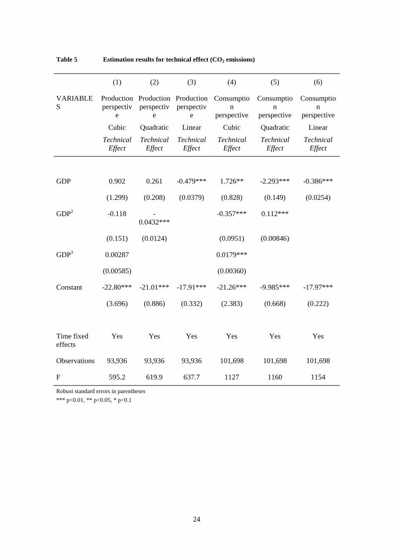
Table 5 presents the results for the aggregate technical effect, i.e. the component of total CO2
emissions which reflect the overall environmental efficiency of the manufacturing sector. We
recall that this component is measured as the by-industry summation of the ‘ratio between the
CO2 emissions of industry i and the consumption of manufacturing goods of industry i.’ By
analysing this component, we can employ all three different approaches for measuring
emissions and the material impact of the manufacturing sector.
-.15 -.1 -.05 0 .05 .1
Wood and Paper
Transport Equipment
Textiles and Wearing Apparel
Recycling
Petroleum, Chemical and Non-Metallic Mineral Products
Other Manufacturing
Metal Products
Food & Beverages
Electrical and Machinery
24
Table 5 Estimation results for technical effect (CO2 emissions)
(1) (2) (3) (4) (5) (6)
VARIABLE
S
Production
perspectiv
e
Cubic
Technical
Effect
Production
perspectiv
e
Quadratic
Technical
Effect
Production
perspectiv
e
Linear
Technical
Effect
Consumptio
n
perspective
Cubic
Technical
Effect
Consumptio
n
perspective
Quadratic
Technical
Effect
Consumptio
n
perspective
Linear
Technical
Effect
GDP 0.902 0.261 -0.479*** 1.726** -2.293*** -0.386***
(1.299) (0.208) (0.0379) (0.828) (0.149) (0.0254)
GDP2 -0.118 -
0.0432***
-0.357*** 0.112***
(0.151) (0.0124) (0.0951) (0.00846)
GDP3 0.00287 0.0179***
(0.00585) (0.00360)
Constant -22.80*** -21.01*** -17.91*** -21.26*** -9.985*** -17.97***
(3.696) (0.886) (0.332) (2.383) (0.668) (0.222)
Time fixed
effects
Yes Yes Yes Yes Yes Yes
Observations 93,936 93,936 93,936 101,698 101,698 101,698
F 595.2 619.9 637.7 1127 1160 1154
Robust standard errors in parentheses
*** p<0.01, ** p<0.05, * p<0.1

25
Table 6 Estimation results for technical effect (material consumption)
(1)
Consumption
perspective
(2)
Consumption
perspective
(3)
Consumption
perspective
VARIABLES Cubic
Technical effect
Quadratic
Technical effect
Linear
Technical effect
GDP 4.486*** -1.320*** -0.144***
(0.592) (0.120) (0.0206)
GDP2 -0.608*** 0.0687***
(0.0690) (0.00671)
GDP3 0.0258***
(0.00265)
Constant -24.63*** -8.342*** -13.26***
(1.684) (0.543) (0.181)
Time fixed effects
Observations 101,698 101,698 101,698
F 1243 1312 1310
Robust standard errors in parentheses
*** p<0.01, ** p<0.05, * p<0.1
Both estimation results and especially Figures A3 to A5 in the appendix highlight that the
aggregate technical component decreases with income level. In addition, as seen in Figure 15,
sector heterogeneity is quite strong: the underlying hypothesis that technological change
increases aggregate manufacturing environmental productivity is not refuted. We recall here that
in Equation 1, the technological component is obtained by aggregating the different degrees of
environmental efficiency by industry. Interestingly, decomposing the aggregate value at
industry level also does not alter the main findings in this case. The individual coefficients are
always negative.

26
Figure 15 Sector-specific elasticity (linear) of environmental pressure intensity in relation to
GDP per capita (from fixed effect estimates including year dummies)
Source: Authors’ elaboration based on the Eora Multi-Region Input-Output database (Lenzen et al., 2012; Lenzen et
al., 2013) and World Development Indicators (World Bank, 2017).
6. Conclusions
This study analysed the relationship between GDP and environmental impacts, namely CO2
emissions and indirect material use. It focused on the manufacturing sector at the global scale.
The analyses were based on a full dynamic perspective. It thus addressed the issue of
sustainable development by looking at structural change and technology/efficiency components,
as well as scale-income effects.
Building on the IDR, decomposition analyses and a panel econometric analysis were used to
analyse the 1995-2013 series. We note that 1995-2013 is a period that witnessed the great bulk
of high growth jumps in developing and emerging countries and the global recession of 2008-
2009. In terms of environmental policy, the period includes the Kyoto Protocol of 1997 and its
ratification in many countries. The period additionally includes the implementation of many key
climate and waste policies, especially in in the EU.
-.8 -.6 -.4 -.2 0
Wood and Paper
Transport Equipment
Textiles and Wearing Apparel
Recycling
Petroleum, Chemical and Non-Metallic Mineral Products
Other Manufacturing
Metal Products
Food & Beverages
Electrical and Machinery
Elasticity between CO2(prod perspective)/VA and GDP pc
Elasticity between CO2(cons perspective)/FD and GDP pc
Elasticity between material use(cons perspective)/FD and GDP pc
27
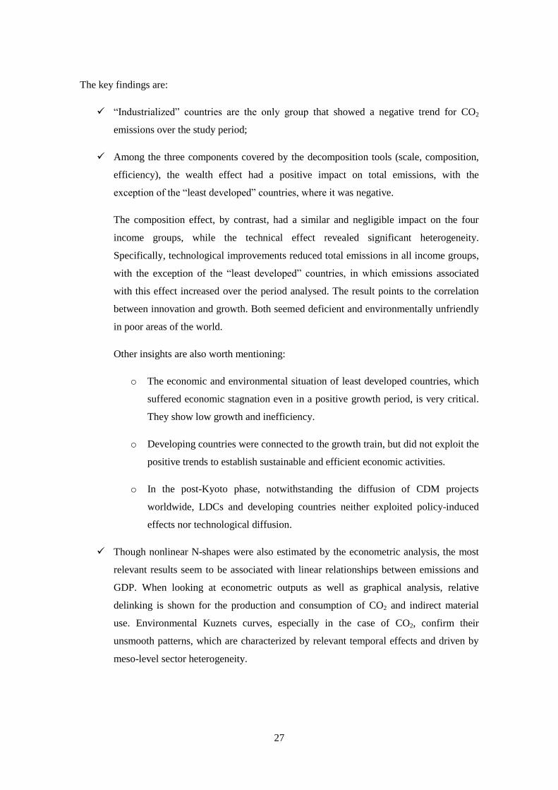
The key findings are:
“Industrialized” countries are the only group that showed a negative trend for CO2
emissions over the study period;
Among the three components covered by the decomposition tools (scale, composition,
efficiency), the wealth effect had a positive impact on total emissions, with the
exception of the “least developed” countries, where it was negative.
The composition effect, by contrast, had a similar and negligible impact on the four
income groups, while the technical effect revealed significant heterogeneity.
Specifically, technological improvements reduced total emissions in all income groups,
with the exception of the “least developed” countries, in which emissions associated
with this effect increased over the period analysed. The result points to the correlation
between innovation and growth. Both seemed deficient and environmentally unfriendly
in poor areas of the world.
Other insights are also worth mentioning:
o The economic and environmental situation of least developed countries, which
suffered economic stagnation even in a positive growth period, is very critical.
They show low growth and inefficiency.
o Developing countries were connected to the growth train, but did not exploit the
positive trends to establish sustainable and efficient economic activities.
o In the post-Kyoto phase, notwithstanding the diffusion of CDM projects
worldwide, LDCs and developing countries neither exploited policy-induced
effects nor technological diffusion.
Though nonlinear N-shapes were also estimated by the econometric analysis, the most
relevant results seem to be associated with linear relationships between emissions and
GDP. When looking at econometric outputs as well as graphical analysis, relative
delinking is shown for the production and consumption of CO2 and indirect material
use. Environmental Kuznets curves, especially in the case of CO2, confirm their
unsmooth patterns, which are characterized by relevant temporal effects and driven by
meso-level sector heterogeneity.

28
The estimations of industry-by-industry income-CO2 elasticities show a strong
monotonic relationship between income and CO2 (production and consumption
perspectives) and indirect material consumption;
The detailed component-by-component analysis shows that (i) the scale effect is
relevant as expected, (ii) the relationship between the composition effect and GDP has a
negative slope: the manufacturing sector becomes greener as income increases, (iii)
technological change has been able to increase aggregate manufacturing environmental
productivity.

29
References
Aghion, P., Dechezleprêtre, A., Hemous, D., Martin, R., & Van Reenen, J. (2016). Carbon
taxes, path dependency, and directed technical change: Evidence from the auto industry.
Journal of Political Economy, 124(1), 1-51.
Antonioli, D., Borghesi, S., & Mazzanti, M. (2016). Are regional systems greening the
economy? Local spillovers, green innovations and firms’ economic performances.
Economics of Innovation and New Technology, 25(7), 692-713.
Borghesi, S., Cainelli, G., & Mazzanti, M. (2015). Linking emission trading to environmental
innovation: evidence from the Italian manufacturing industry. Research Policy, 44(3), 669-
683.
Borghesi, S., Crespi, F., D’Amato, A., Mazzanti, M., & Silvestri, F. (2015). Carbon abatement,
sector heterogeneity and policy responses: evidence on induced eco innovations in the EU.
Environmental Science & Policy, 54, 377-388.
Cainelli, G., & Mazzanti, M. (2013). Environmental innovations in services: Manufacturing–
services integration and policy transmissions. Research Policy, 42(9), 1595-1604.
Cainelli, G., Mazzanti, M., & Montresor, S. (2012). Environmental innovations, local networks
and internationalization. Industry and Innovation, 19(8), 697-734.
Cainelli, G., Mazzanti, M., & Zoboli, R. (2013). Environmental performance,
manufacturing sectors and firm growth: structural factors and dynamic
relationships. Environmental Economics and Policy Studies, 15(4), 367-387.
Chao, H. K. (2001). Professor Hendry's Econometric Methodology Reconsidered: Congruence
and Structural Empiricism. In University of Amsterdam. Holland.
Corradini, M., Costantini, V., Mancinelli, S., & Mazzanti, M. (2014). Unveiling the dynamic
relation between R&D and emission abatement: National and sectoral innovation
perspectives from the EU. Ecological Economics, 102, 48-59.
Costantini, V., & Mazzanti, M. (Eds.). (2012). The dynamics of environmental and economic
systems: innovation, environmental policy and competitiveness. Springer Science &
Business Media.
Costantini, V., & Sforna, G. (2014). Do bilateral trade relationships influence the distribution
of CDM projects?. Climate policy, 14(5), 559-580.
Costantini, V., Mazzanti, M., & Montini, A. (2013). Environmental performance, innovation
and spillovers. Evidence from a regional NAMEA. Ecological Economics, 89, 101-114.
Gilli, M., Mazzanti, M., & Nicolli, F. (2013). Sustainability and competitiveness in
evolutionary perspectives: Environmental innovations, structural change and economic
dynamics in the EU. The Journal of Socio-Economics, 45, 204-215.
Hendry, D. F. (1980). Econometrics-alchemy or science?. Economica, 387-406.
30
Lenzen, M., Kanemoto, K., Moran, D. and Geschke, A. (2012). Mapping the Structure of the
World Economy. Environmental Science and Technology, 46(15), pp. 8374–8381.
Lenzen, M., Moran, D., Kanemoto, K. and Geschke, A., (2013). Building Eora: A Global
Multi-Region Input–Output Database at High Country and Sector Resolution. Economic
Systems Research, 25(1), pp. 20–49.
Martin, R., De Preux, L. B., & Wagner, U. J. (2014). The impact of a carbon tax on
manufacturing: Evidence from microdata. Journal of Public Economics, 117, 1-14.
Mazzanti, M., & Montini, A. (2010). Embedding the drivers of emission efficiency at regional
level—Analyses of NAMEA data. Ecological Economics, 69(12), 2457-2467.
Mazzanti, M., & Montini, A. (Eds.). (2010). Environmental efficiency, innovation and
economic performances (Vol. 25). Routledge.
Mazzanti, M., Marin, G., Mancinelli, S., & Nicolli, F. (2015). Carbon dioxide reducing
environmental innovations, sector upstream/downstream integration and policy: evidence
from the EU. Empirica, 42(4), 709-735.
Mazzanti, M., Montini, A., & Marin, G. (2011). Linking NAMEA and Input output
for'consumption vs. production perspective'analyses (No. 201108).
Mazzanti, M., Musolesi, A., & Zoboli, R. (2010). A Bayesian Approach to the estimation of
EKC for CO2. Applied Economics, 42(18), 2275-2287.
Musolesi, A., & Mazzanti, M. (2014). Nonlinearity, heterogeneity and unobserved effects in
the carbon dioxide emissions-economic development relation for advanced
countries. Studies in Nonlinear Dynamics & Econometrics, 18(5), 521-541.
World Bank (2017). World Development Indicators. Available at:
https://data.worldbank.org/data-catalog/world-development-indicators [Accessed January 2,
2017].
31
Appendix
Figure A1 Fitted values of the relationship between the wealth effect per capita and GDP per
capita with estimated parameters
Source: Authors’ elaboration based on the Eora Multi-Region Input-Output database (Lenzen et
al., 2012; Lenzen et al., 2013) and World Development Indicators (World Bank, 2017).
Figure A2 Fitted values of the relationship between the aggregate composition component
and GDP per capita with estimated parameters
Source: Authors’ elaboration based on the Eora Multi-Region Input-Output database (Lenzen et al. 2012; Lenzen et
al. 2013) and World Development Indicators (World Bank 2017).
13
13.5
14
14.5
log o
f per
capita m
anif
. goods c
onsum
ption (
fitt
ed
valu
es)
8.8 8.9 9 9.1 9.2Log of GDP per capita (USD)
-20.3
-20.2
-20.1
-20
-19.9
log o
f per
capital secto
rial share
of
manuf.
goods c
ons.
over
the t
ota
l (f
itte
d v
al.)
8.7 8.8 8.9 9 9.1 9.2Log of GDP per capita (USD)

32
Figure A3 Fitted values of the relationship between the aggregate technical effect and GDP
per capita with estimated parameters (production perspective)
Source: Authors’ elaboration based on the Eora Multi-Region Input-Output database (Lenzen et al., 2012; Lenzen et
al., 2013) and World Development Indicators (World Bank, 2017).
Figure A4 Fitted values of the relationship between the aggregate technical effect and GDP
per capita with estimated parameters (consumption perspective)
Source: Authors’ elaboration based on the Eora Multi-Region Input-Output database (Lenzen et al., 2012; Lenzen et
al., 2013) and World Development Indicators (World Bank, 2017).
-23.5
-23
-22.5
-22
log o
f (C
O2 e
mis
sio
n/m
anif.
goods c
onsum
ption)
per
capita (
fitt
ed v
al,)
8.7 8.8 8.9 9 9.1 9.2Log of GDP per capita (USD)
Production perspective
-22.5
-22
-21.5
-21
-20.5
Log o
f (C
O2 e
mis
sio
ns/m
anif.
goods c
onsum
ption)
per
capita (
fitt
ed v
al.)
8.7 8.8 8.9 9 9.1 9.2Log of GDP per capita (USD)
Consumption perspective

33
Figure A5 Fitted values of the relationship between the aggregate technical effect and GDP
per capita with estimated parameters (indirect material consumption)
Source: Authors’ elaboration based on the Eora Multi-Region Input-Output database (Lenzen et al., 2012; Lenzen et
al., 2013) and World Development Indicators (World Bank, 2017).
-16
-15.5
-15
-14.5
Log o
f (i
ndir
ect
mate
rial cons./
manif.
goods c
ons)
per
capita (
fitt
ed v
alu
es)
8.7 8.8 8.9 9 9.1 9.2Log of GDP per capita (USD)

Vienna International Centre · P.O. Box 300 9 · 1400 Vienna · AustriaTel.: (+43-1) 26026-o · E-mail: [email protected]