Cities xxx (xxxx) xxx

Please cite this article as: Xin Li, Cities, https://doi.org/10.1016/j.cities.2021.103482

0264-2751/© 2021 Elsevier Ltd. All rights reserved.

The six dimensions of built environment on urban vitality: Fusion evidence from multi-source data

Xin Li a, Yuan Li b, Tao Jia c,*, Lin Zhou a, Ihab Hamzi Hijazi d

a School of Urban Design, Wuhan University, Wuhan, China b School of Architecture and Civil Engineering, Xiamen University, Xiamen, China c School of Remote Sensing and Information Engineering, Wuhan University, Wuhan, China d Urban Planning Engineering Department, An-Najah National University, Nablus, Palestine

A R T I C L E I N F O

Keywords: Urban vitality Built environment Community Big data Wuhan

A B S T R A C T

Long-standing attention has been given to urban vitality and its association with the built environment (BE). However, the multiplicity and complex impacts of BE factors that shape urban vitality patterns have not been fully explored. For this purpose, multisource data from 1025 communities in Wuhan, China, were combined to explore the BE vitality nexus. A deep learning method was explored to segment street-view images, on which a composite indicator of urban vitality was developed with social media data. Then, six dimensions of BE factors, neighbourhood attributes, urban form and function, landscape, location, and street configuration, were incor-porated into a spatial regression model to systematically examine the composite influences. The results show that population density, community age, open space, the sidewalk ratio, streetlights, shopping and leisure density, integration, and proximity to transportation are positive factors that induce urban vitality, whereas the effects of road density, proximity to parks, and green space have the opposite results. This study contributes to an improved understanding of the BE nexus. Managerial implications for mediating the relationship between planning policies and urban design strategies for the optimization of resource allocation and promotion of sustainable development are discussed.

1. Introduction

The unprecedented worldwide urbanization since the mid-20th century has resulted in profound changes in the socioeconomic and built environments in the cities of major industrial countries. Taking one of the largest emerging economies, e.g., China, which has transitioned from industrialization to postindustrialization, has experienced the large-scale demolition of old communities, urban villages, and slums under the pressure of intensified land use in urban centres (Batty, 2016). The implementation of some strategies to improve the cityscape and living conditions has not only reduced the diversity of urban fabric but also brought unanticipated changes to social networks and caused consequences, such as social segregation, population loss, and residen-tial vacancy, threatening the integrity and sustainability of the current urban system (Batty, 2016; Deng & Ma, 2015). Therefore, the appeal for a more vibrant urban life continues to increase, as is believed to promote favourable health and safety outcomes (Braun & Malizia, 2015).

Particularly in the context of the pandemic crisis of coronavirus 2019 (COVID-19), which has infected more than 105 million people and caused 2.3 million deaths worldwide as of January 2021, it is even more necessary to maintain a balance between resource capacities and so-cioeconomic developments to prevent a global economic recession caused by the associated lockdown (Dizdaroglu, 2017; Lu & Ke, 2017). In this sense, more efforts should be made to adjust and optimize the human-place relationship. Therefore, investigating urban vitality in depth and the influencing factors contributes to a better understanding of the intricate relationship between urban dynamics and socioeconomic order (Lang, Chen, & Li, 2015; Li, Shen, & Hao, 2016).

Social communities have long yearned for the renewed livelihood of public spaces (Tang & Long, 2019). In particular, planners are concerned with various qualities of life that influence people's well-being (Carmona & Sieh, 2004). The existing literature on quality of life often includes discussions on safety (Shach-Pinsly, 2019; Shach-Pinsly & Ganor, 2021), walking environment (Ewing & Handy, 2009), visual qualities (Tang &

* Corresponding author. E-mail addresses: li-xin@whu.edu.cn (X. Li), liyuan79@xmu.edu.cn (Y. Li), tao.jia@whu.edu.cn (T. Jia), 2014301530136@whu.edu.cn (L. Zhou), eehab@najah.

edu (I.H. Hijazi).

Contents lists available at ScienceDirect

Cities

journal homepage: www.elsevier.com/locate/cities

https://doi.org/10.1016/j.cities.2021.103482 Received 23 February 2021; Received in revised form 9 August 2021; Accepted 25 September 2021

Cities xxx (xxxx) xxx

2

Long, 2019), public life (Gehl & Svarre, 2013), etc. It is well accepted that community vibrancy, a component of essential quality of life, plays an important role in residents' overall well-being since increasing ideals for rebuilding a lively city have resonated in related urban planning theories, e.g., new urbanism and smart growth, since the 1990s (Grant, 2002; Sternberg & Ernest, 2000). It is believed that places with a high level of vitality often embody extra quality of life through the exhibition of social interactions, public activities, and sense of place, all of which in turn regenerate the significant characteristics of a place (Krier, 2009; Montgomery & John, 1998).

Despite the difficulty of achieving a consensus on the definition of urban vitality, it is reflected in human-space interactions in different places and times (Li et al., 2016). Although the formation of quality of life often originates from a good living environment, well-designed urban form, fully connected public spaces, and easy access to life ser-vices (Jin et al., 2017), determining additional essential factors that influence urban vitality in different contexts has always been a goal of researchers. For instance, many investigations have been conducted to test the association between street configuration and socioeconomic activities within the theoretical framework of space syntax (Hillier & Hanson, 1984), which have revealed the important role of accessibility in facilitating progressive urban development in different contexts (Alalouch, Al-Hajri, Naser, & Al Hinai, 2019; Grant, 2002; Jiang, Alves, Rodrigues, Ferreira, & Pereira, 2015; Ozbil, Peponis, & Stone, 2011; Zeng, Song, He, & Shen, 2018). In addition, Porta et al. (2012) used economic activities as a proxy for urban vitality to discuss its association with street centrality measures (Porta et al., 2012). Omer and Goldblatt (2016) investigated eight Israeli cities and revealed a correlation be-tween retail activities and street configuration (Omer & Goldblatt, 2016), and they found that office building density is correlated with street configuration (Kim & Sohn, 2002). In terms of other BE attributes, an increasing number of studies have investigated how various combi-nations of urban form metrics (e.g., mixed land use, accessibility, den-sity, and external traffic systems) contribute to characterizing neighbourhood vibrancy (Wu, Ta, Song, Lin, & Chai, 2018; Yue, Zhuang, Yeh, & Xie, 2016). In practical terms, several planning principles, e.g., mixed use, small blocks, and intensive development, have been pro-posed to cultivate urban vitality.

Both practical and theoretical investigations of urban vitality within the Western world have revealed its crucial effects on sustainable urban development, and these studies have tremendously improved our un-derstanding of the complicated sociospatial relationships between BE factors and urban vitality. However, some important yet incompletely solved issues remain. For instance, although much scholarly attention has been given to Western experiences, exploration of empirical con-sequences in the context of developing countries is lacking, particularly in China, where residential living modes are different (Weng et al., 2019). More importantly, although traditional methods relying on field surveys are still valuable, they are no longer suitable for large-scale investigations, especially in situations with limited time and resources. The automatic quantitative investigation of urban vitality in large areas has encountered difficulties. Exploring vitality issues with advanced methods, particularly with multisource big-data techniques, is impera-tive for researchers and planners to enrich the existing literature and practices. In addition, to the best of our knowledge, relatively limited BE dimensions have been considered in previous studies, whereas the multiplicity of BEs and the complex impacts of spatial-functional factors that shape the pattern of urban vitality have not been fully explored. Due to data source limitations, it is still difficult to obtain an overview of the whole picture of the composite effects of BE factors on urban vitality without the addition of a rich variety of big data, which might compromise the reliability of the results. For instance, it is still unclear to what extent street configuration provides an independent impetus on urban vitality if many related BE factors are controlled. Moreover, little consideration has been made to reduce the spatial autocorrelation interference among factors, which may compromise the reliability of

estimates (Weng et al., 2019). Along with the development of cutting-edge techniques, such as deep

learning algorithms for image processing and crowdsourcing methods, researchers can explore more intangible qualities, such as urban vitality, in a large geographical area. In this study, we refer to the theory of natural movement to establish a coherent framework linking urban vi-tality and BE factors. As previous studies have been subject to limited sampling strategies and relatively low spatiotemporal resolutions, we attempted to draw support from a new data environment with multiple data sources, which allows researchers to collect large-volume urban data more efficiently (Chen, Zhang, Cui, & He, 2015). With the help of deep learning methods, different categories of human flows can be automatically counted at high resolution. This study enriches the existing body of literature by verifying the composite effects of various BE factors while clarifying the independent effects of street configura-tion, eventually providing improved planning strategies to optimize resource allocation and promote sustainable development (Alalouch et al., 2019).

The remainder of this paper begins with a brief literature review on the concepts of urban vitality, BE factors, and the relevant theories and studies. In the materials section, we introduce the study area, variable measurements, data preparation, and analytical methods. Then, the results are presented. Finally, we discuss the implications of the research findings in combination with the conclusion and research limitations.

2. Literature review

2.1. Urban vitality

Urban vitality often emerges when urban activities interact with spatial entities (Li et al., 2016; Wu, Ta, et al., 2018) and is usually perceived as an essential quality of life in cities (Jin et al., 2017). In Jacobs' (1961) long-standing arguments for making a good neighbour-hood, the concept of vitality was frequently mentioned to describe how a place keeps busy to make people feel vibrant at different times and lo-cations. Recently, Shach-Pinsly (2019) reemphasized Jacobs' impor-tance of increasing the number of people in a public open area, as it not only ensures a sense of personal security in an area but also enhances a city's vitality. To establish a vibrant urban environment, six major conditions need to be noted: density, land use mix, block size, building age, accessibility, and lack of border vacuums (Jacobs, 1961).

According to Lynch (1984), urban vitality is an important indicator to measure how the form of settlement supports people's lives and needs (Lynch, 1984; Maas, 1984). Montgomery and John (1998) attributed successful urban places to street life and the various forms of activities that occur in urban spaces, emphasizing the significance of human ac-tivities for inducing urban vitality and distinguishing good places from others. Several important conditions alike, e.g., the number of people in and around the streets, the presence of small-scale business activities, the uptake of facilities, and the frequency of cultural events and cele-brations, are believed to be applicable to the nourishment of a vibrant atmosphere for a place (Montgomery & John, 1998). A supportive urban environment plays an important role in inducing the continuous pres-ence of people and activities or opportunities (Lynch, 1984; Maas, 1984). Among the essential BE conditions for creating a pleasant urban place, mixed use and density are frequently discussed (Montgomery & John, 1998).

Typically, existing relevant studies have tried to break down urban vitality into measurable aspects. To investigate urban vitality at the neighbourhood level, objective indicators that reflect human conditions have been used. For instance, Wu, Ye, Ren, and Du (2018) used the percentage of out-of-home nonwork activities in which individuals participate within a given distance from the boundary of the neigh-bourhood. Xia, Yeh, and Zhang (2020) proposed using a small catering business to measure a city's daytime vitality (Xia et al., 2020). Recently, social media data and mobile data have also been adopted to

X. Li et al.

Cities xxx (xxxx) xxx

3

characterize urban vitality. For instance, some researchers have used the number of check-ins to measure the degree of neighbourhood vitality (Lu, Huang, Shi, & Yang, 2019). Others have summarized the accumu-lated number of mobile phone users on a working day as a proxy for urban vitality (Yue et al., 2017). Based on the concept of ‘good urban-ism’, some researchers have attempted to compose a composite vitality index that is characterized by a series of street-space qualities: the synergy of safety, security, convenience, continuity, comfort, and attractiveness (Tang & Long, 2019).

Although the convergence of human flows in public urban spaces is often used as an appropriate proxy (Montgomery & John, 1998), it is rare to directly adopt street movements, a concrete embodiment, to investigate vitality more in depth. In theory, Hillier and Penn (1996) noted that cities can be conceptualized as ‘movement economies’, indicating that urban vitality can be measured by accounting for various street movements, as all follow the rule of ‘natural movement’. Initially, pedestrian volume has been counted in field surveys to denote street vitality (Maas, 1984). Later, by comparing the pedestrian volume from field survey data and Baidu street view map data, some researchers confirmed the feasibility of measuring urban vitality using street-view images (Liu, Sheng, & Yang, 2018). Other types of movement have also been explored to provide more evidence of the correlation with urban vitality (Hillier & Iida, 2005; Hillier & Penn, 1996; Lerman, Rofe, & Omer, 2014; McCahill & Garrick, 2008; Sheng, Yang, & Hou, 2015). Therefore, selected street movements, such as those of pedestrians, bi-cycles, motors, buses, and private cars, could represent urban vitality due to their capacity to induce communications and businesses. When investigating an area of manageable scale during a given window period, the street snapshot method is frequently used to determine the density of use, such as usage patterns, pedestrian activities, and vehicles. However, due to the constraints of labour and time consumption, the traditional method of data collection relying on field surveys is not feasible for investigations on a large scale (Filion & Hammond, 2003; Wu, Ta, et al., 2018), while a small sample size and low resolution make it difficult to obtain robust conclusions. With the availability of big data (Wu, Ye, et al., 2018; Yue et al., 2016), it has become possible to collect and process urban vitality data on a relatively large scale (Markusen, 2013).

2.2. BE factors and urban vitality

Within the field of urban studies, BE factors not only profoundly affect the economic development of a city but also play an important role in associating urban vitality with planning policies (Li & Liu, 2018). Many studies have addressed various aspects that affect urban vitality and quality of life, including safety, walkability, and visual quality. A list of up to fifty-one perceptual qualities related to BE factors, such as imageability, enclosure, human scale, transparency and complexity, has even been proposed, and many designers and practitioners have been expecting to translate these concerns into design vocabularies (Ewing & Handy, 2009), which will help facilitate the materialization of the concept of good urban spaces t (Ewing & Clemente, 2013). As the basis of Maslow's theory of the hierarchy of needs, a sense of security has a significant influence on people's lives and needs, so urban design ought to provide enough sense of personal security before a place becomes vibrant (Shach-Pinsly, 2019). For instance, it was found that some physical characteristics such as streetlights and urban aesthetics often affect the way people perceive risks in public spaces; therefore, they should be integrated into urban planning and design (Foster, Wood, Christian, Knuiman, & Giles-Corti, 2013). In addition to synergy in safety, Tang and Long (2019) emphasized the role of the quality of street space, i.e., convenience, continuity, comfort, and attractiveness, all of which could contribute to shaping public spaces with a lively atmo-sphere and enhance the frequency of outdoor activities, thus affecting users' behaviour.

With regard to vitality-related issues, the urban form is also the main

focus of planners and urban researchers. For instance, Conzen (1960) emphasized the importance of urban texture elements, including streets, blocks, plots, and buildings (Conzen, 1960; Whitehand, Samuels, & Conzen, 2009). Song, Merlin, and Rodriguez (2013) summarized 27 sets of urban form elements, which could be further categorized into three groups: permeability, accessibility, and variety (Song et al., 2013). To describe downtown vibrancy in large US cities, Braun and Malizia (2015) developed a composite index based on the combination of spe-cific features of urban form, e.g., the floor area ratio (FAR), compact-ness, density, local connectivity, destination accessibility, and land use mixture (Braun & Malizia, 2015). Similarly, Zeng et al. (2018) adopted density features (e.g., roads, intersections, and buildings) and location features (e.g., distance to shops and tourist attractions) for a comparison between Chicago and Wuhan in terms of the outcome measure of urban vitality (Zeng et al., 2018).

From the accessibility perspective, the space syntax method is often used to investigate the associations among street configuration, urban function, and human activities, providing valuable evidence for under-standing the dynamic mechanism of urban vitality. For instance, re-searchers have observed that streets with a higher degree of integration tend to have greater pedestrian volumes (Foltete & Piombini, 2007; Hajrasouliha & Yin, 2015; Lerman et al., 2014); a possible explanation is that travel distances are shorter between places with well-connected linkages (Frank, 2000), and the core argumentation is based on the theory of natural movement, which affirms that various urban phe-nomena are intrinsically influenced by the directness and accessibility of routes within a street network (Handy, Cao, & Mokhtarian, 2005; Hillier & Hanson, 1984; Hillier, Hanson, & Graham, 1987; Hillier, Yang, & Turner, 2012). Natural movement refers to the ability of the street configuration itself to shape the pattern of human flows rather than relying on only the presence of specific magnets. It considers the street configuration as a primary force that modulates pedestrian flows, positing that highly connected streets are likely to be more accessible from surrounding locations and thus draw more human flows, as can be intuitively discerned in many public open spaces (Dhanani, Tarkhanyan, & Vaughan, 2017; Hillier, Penn, Hanson, Grajewski, & Xu, 1993; Karimi, 2012; Omer & Goldblatt, 2016). Accordingly, street vitality should also be an innate characteristic of natural movement (Hillier et al., 1993; Hillier & Penn, 1996).

On basis of the discussion above, there is also a growing body of literature discussing how the street configuration of a city affects land use, urban function, and facility distribution, all of which can be regarded as potential contributors to urban vitality. For instance, plan-ners often regard multifunctional land use as a beneficial urban design strategy that physically integrates various functions and facilitates social connections, which contribute to promoting urban vibrancy and yield socioeconomic benefits (Katz, Scully, & Bressi, 1994; Koster & Rou-wendal, 2012). The effect of spatial configuration characteristics on land prices has been measured (Lee & Kim, 2009). Kim and Sohn (2002) found that syntactic indicators, e.g., integration, connectivity, and control, present a strong correlation with urban function, particularly the density of office buildings (Kim & Sohn, 2002). Even in different contexts, the association between street configuration and the avail-ability of commercial destinations is significant (Liu, Wei, Jiao, & Wang, 2016; Omer & Goldblatt, 2016; Tsou & Cheng, 2013; Wang, Chen, Xiu, & Zhang, 2014). Similar findings could be observed in Bergen when some researchers investigated how urban transformation takes place in the central area, showing that street layout affects multiple urban phe-nomena, such as commercial activities, building density, and mixed functions (Koning, Nes, Ye, & Roald, 2017). Table 1 summarizes the international literature on related topics.

However, based on the conceptual frameworks and previous find-ings, some limitations exist, which calls for further investigations of the comprehensive effects of multidimensional BE factors on urban vitality outcomes. For instance, due to limited data sources, previous studies have mainly focused on analyzing the pairwise relationships between

X. Li et al.

Cities xxx (xxxx) xxx

4

Table 1 Literature on BEs and vitality-related outcomes.

Study area and scale Outcomes Methods BE variables Main findings

17 neighborhoods in Beijing (Wu, Ta, et al., 2018)

Neighbourhood vibrancy

Multi-level regression

Inter circulation: street intersection, perimeter of blocks, blocks per household, length of cul-de-sacs; External traffic: distance to bus stop/subway station; Density: FAR; Land use mix: Shannon diversity of land use; Accessibility: distance to retail site/commercial site/park;

Positive correlation: density and mixed land use; Negative correlation: external traffic systems;

2 counties of NY State, US (Deng & Ma, 2015)

Residential vacancy Stepwise OLS regression, Logistic regression

Housing age; Distance to: brownfields/bus stop/food/ commercial/community service/farmers market/ grocery store/industrial/recreation/public service; Distance to: rail/rivers/major road; Percentage of parks or recreation facilities; NDVI;

Positivel correlation: NDVI, park/ recreation distance, and grocery distance, and bus stop distance.

150 transport zones and neighborhoods in Madrid, Spain ( Lamíquiz & Lopez-Domínguez, 2015).

Percentage of walking trips (walking rate)

Multivariate regression

Geometry: street length, street density, cul de sac density; Accessibility: configurational accessibility (integration, intelligibility); Density: density of residents/ residents+jobs+students/retail food/retail unit/ retail job, land use mix; Distance to city centre;

Positive correlation: resident density, retail food density, and job density. Negative correlation: integration, street length, street desnity, and distance to city centre.

653 cities in China (Jin et al., 2017) Residential vitality Score of multiple components

Road junctions, Point of interest (POI), Location based service data (LBS)

Residential vitality is associated with three components, i.e. road density, POI, and LBS.

Communities in Chicaga US and Wuhan China (Zeng et al., 2018)

Urban vibrancy DALD model Density: road density, building density; Accessibility: distance to schools/hospitals/shops/ tourist attractions; Livability: number of banks/food service/leisure and recreation/services for beauties and cars; Diversity: Shannon diversity of land use

Chicago is superior in accessibility and diversity, whereas Wuhan has better density and livability. communities around the scenic spots or with large areas are highly likely to be influenced by neighbors

133 to streets and 63 pedestrian zones in the donwndown area of Santiago in Chile (Lunecke & Mora, 2018)

Urban vibrancy Counting based descriptive analysis

Configuration structure of streets, pedestrian zones, commercials.

Pedestrian network introduces a progressive differentiation of pedestrian flows into the urban block

4 morphologies at a one hectare in Mumbai, India (Dovey & Pafka, 2014)

Streetlife vitality Theoretical review FAR, coverage, site area; Open space; Number of intersections, block area/perimeter;

Density enables high levels of streetlife and walkable access to diverse amenities.

1090 individual visits to 324 urban parks in Brisbane, Australia ( Shanahan, Lin, Gaston, Bush, & Fuller, 2015)

Percentage of parks visited

Linear mixed models

Tree cover; remnant vegetation cover Tree cover and remnant vegetation cover have limited overall influence on park visitation rates.

1823 samples in Seoul, South Korea ( Sung & Lee, 2015)

Walking activity Multi-level regression

Land use mix; Block size; Distance from building entrance to street; Building age; Concentration: all building desnity, building desnity for daily activity use, office building density; Accessibility: Distance to the CBDs/bus stop/rail station; Border vacuums: Distance to river or stream/ railway

Positive correlation: intersection density, building age, building density, proximity to border vacuums.

Bat Yam of TelAviv District, Iseral ( Lerman et al., 2014)

Pedestrian movement Bivariate correlation

Global integration/Choice; Local integration/ Choice; Connectivity; Angular mean depth; Normalized angular choice; Commercial fronts; Bus stop;

Pedestrian movement is positively associated with the space syntax variables

Downtown and Midtown of Atlanta, and Virginia Highland neighbourhood, US (Ozbil et al., 2011)

Pedestrian movement Multivariate regression

Connectivity: metric reach, block area; Land use: residential area, non-residential area (office, retail, institution, recreation, industrial);

Positive correlation: metric reach, non-residential area

302 street segments in Buffalo, US ( Hajrasouliha & Yin, 2015)

Pedestrian volume Structural equation modelling (SEM)

Integration; Intersection density; Land use mix; Job density;

All the explanatory BE variables are positive correlated with pedestrian volume. Population density presents non- significant correlation.

X. Li et al.

Cities xxx (xxxx) xxx

5

urban vitality and a few aforementioned BE factors, whereas the po-tential links among broader BE dimensions, as can be observed in daily life, have not been fully taken into account. For instance, certain urban functions that rely heavily on a large number of passers-by, such as commercial, retail, food, and entertainment functions, prefer to be located on the ground floor or in districts with better accessibility. In turn, a service-based location might also become a magnet to attract more people according to the law of natural movement, which assumes that highly accessible street segments might generate high concentra-tions of attractive land use, particularly nonresidential economic and service activities (Hillier et al., 1993; Hillier & Penn, 1996). As a result, the cohesive influence of urban functions might blur the effects of street configuration on urban vitality, leading to either inflated or under-estimated estimations (Vaughan, Jones, Griffiths, & Haklay, 2010). In addition, most of the aforementioned studies adopted nonspatial regression models that abide by the assumption of sample indepen-dence, whereas some geographic events, such as those selected for investigation in this study, are often affected by the characteristics of

neighbouring locations. Neglecting the spatial effect might introduce unexpected bias. It is therefore urgently necessary to employ more BE factors for testing while considering the spatial interference from sur-rounding units.

Recently, there have been discussions that greenery has a positive effect on urban activities, although debates on the mixed effects still exist (Gavrilidis, Ciocanea, Nita, Onose, & Nastase, 2016; Shanahan et al., 2015). As an important BE factor, the green ratio is adopted in this study for validation because the role of green spaces in improving the quality of urban life is discernible, particularly when green spaces are easily reachable by the population (Lopes & Camanho, 2013). Moreover, other potential influences might exist to blur the independent effect of BE factors on urban vitality and should also be taken into consideration. For instance, since population density has been thoroughly determined to be an appropriate indicator of human activities (Sung, Go, & Chang, 2013; Wang & Guldmann, 1996; Zeng et al., 2018), it constitutes the fundamental condition of urban vitality. Aged buildings located in the central urban area in the context of developing countries are important

Fig. 1. The study area and the spatial distribution of street view data and POIs.

X. Li et al.

Cities xxx (xxxx) xxx

6

for depicting the community characteristics that might potentially in-fluence urban vitality nearby. In addition, land prices are employed to limit the bias of potential residential self-selection; i.e., individuals purposely decide where to live in cities on the basis of their socio-demographic status and affordability (Cao, Mokhtarian, & Handy, 2009). In turn, this phenomenon may shape the settlement and activities of the local area, because some researchers have indicated that area- level land prices might affect household wealth (Xiao, Lu, Guo, & Yuan, 2017).

3. Materials

3.1. Study area

In this case, Wuhan, which is the political and economic centre of Hubei Province and one of the national core cities of China (Fig. 1), is selected as the study area. Wuhan covered an area of 8569 km2 and had a population of 11.21 million at the end of 2019. The prosperity of modern industries in Wuhan has created an abundance of job opportu-nities that have attracted an influx of people. After decades of steady economic growth, Wuhan has long ranked among the top ten megacities of China in terms of GDP, reaching 1561.6 billion RMB in 2020 after a three-month lockdown despite the great impact of COVID-19. In this study, we focus on the most urbanized region within the Third Ring, which consists of seven administrative districts (four on the northern side of the Yangtze River and three on the southern side), covering an area of 525 km2. Within the study area, the statistical analysis is based on 1025 community blocks (shequ or juweihui), which are the smallest administrative units for population censuses and the supply of public services in urban China.

3.2. Data sources

In this study, six types of data were used: street vitality data, POI data, urban administration map data, community attribute data, remote sensing image data, and community population data (Table 2). The urban vitality data were based on the detection of featured street ele-ments, such as pedestrians, bicycles, motors, buses, private cars, and trucks, via street-view images from Baidu, which is the largest search engine provider in China. Its application program interface (API) pro-vides the most comprehensive service with adequate coverage of street- view images and various types of points of interest (POIs) within the study area. POIs refer to the point-like geospatial data of a real geographical entity from a spatial perspective for the representation of all types of functional facilities in a city (such as shops, banks, schools, and office buildings), which include descriptive location-based infor-mation, categories, and other attributes. There have been increasing attempts to combine the spatial distribution of these factors with other categorical properties to investigate human perception and behaviour

because of the widespread coverage, large volume, easy accessibility, and high degree of accuracy of these data (Bakillah, Liang, Mobasheri, Arsanjani, & Zipf, 2014; Huang, Gartner, & Turdean, 2013). Batty (2010) noted that information and communication technology (ICT) has recently provided more opportunities to access new growing data sources that enable us to observe and examine cities at a fine scale and gain a better understanding of the pulse of cities. Given this background, utilizing POI data to estimate land use is reasonable and helpful, espe-cially given the emerging public availability of POI data within map- based applications.

The community attribute data were obtained from two major online real estate networks, Soufang and 58-Tongcheng, which provide hous-ing prices, community ages, floor-area ratios, open space rates, etc. Population data were obtained from the Wuhan Land Resources and Planning Information Center, and supplementary data were obtained from the Gridded Population of the World. A digital map containing the Wuhan administrative boundary and related street network was ob-tained from OpenStreetMap, which is an open-access and volunteer GIS platform. Other thematic maps were obtained from the Wuhan Land Resources and Planning Information Center. The remote sensing Landsat image data were obtained from the National Earth System Science Data Center. In general, these variables could be categorized into six groups: neighbourhood attributes, urban form, facility, location, landscape, and accessibility.

3.3. Measurements

3.3.1. Vitality indicators The street-view images used in this study were acquired in May

2019, and the data were obtained by requesting the Baidu API in 2020. To have enough sampling points and ensure a reasonable computation time for analysis, observations were set up approximately every 30 m along the road to cover the streetscape. Ultimately, a total of 67,761 street-view images were collected within the study area. Then, a se-mantic segmentation technique based on deep learning was applied to segment street-view images into common ground objects. For training, a fully convolutional neural network (FCN) was adopted based on a collection of ADE20k datasets, which consist of more than 25,000 an-notated images (Zhou et al., 2017). Then, we input the street-view im-ages into the trained network, as illustrated in Fig. 2. Ultimately, six categories of street elements could be determined for counting, pedes-trians, bicycles, motor-vehicles, buses, private cars, and trucks, and the values were summed to denote urban vitality after normalization, with the mean equal to 0 and the standard deviation equal to 1.

To further take the temporal dimension into account, we enlarged the data source to ensure a more stable estimate. Since the increase in social media applications on mobile devices (e.g., Facebook, Tweeter, and Weibo) has encouraged an increasing number of people to share their location information on the internet, a large volume of open check- in records have been provided, which reflect people's interests or pref-erences in a certain place. A massive amount of these spontaneous location-based data can reflect the popularity of a certain place for a given time span. Therefore, it is reasonable to combine social media data with street view data to compose a composite indicator of urban vitality, denoting a more comprehensive measure of various types of activities and temporal dimensions. Eventually, a one-month record of 114,145 Weibo check-ins was collected within the study area. The counting of check-in data within each community was also normalized, with a mean equal to 0 and a standard deviation equal to 1. Then, the composite measure of urban vitality was obtained by calculating the average mean of the check-in data and street view data.

3.3.2. Urban facilities and land use POI data contain rich location-based information and other attri-

butes from a spatial perspective (Bakillah et al., 2014). Due to the ad-vantages of their widespread coverage, large volume, easy accessibility,

Table 2 Data sources used in this study.

Data Data source

Street vitality Baidu Map (http://lbsyun.baidu.com/) POI data Baidu Map (http://lbsyun.baidu.com/) Weibo check-ins SINA (https://open.weibo.com) Maps of urban

administration OpenStreetMap (https://www.openstreetmap.org)

Community attributes Soufang (https://wh.sofang.com/); 58-Tongcheng (https://wh.58.com/)

Landsat RS image National Earth System Science Data Center (htt p://www.geodata.cn/)

Population Bureau of Wuhan Natural Resource and Planning Gridded Population of the World (http://sedac.ciesi n.columbia.edu/gpw)

Data: social sensing; remote sensing; crowd source; government.

X. Li et al.

Cities xxx (xxxx) xxx

7

and high degree of accuracy, POIs have increasingly emerged as powerful tools to reflect the distribution of urban function and investi-gate human perceptions or behaviors. Within the study area, approxi-mately 0.28 million POIs were collected and regrouped into nine frequently applied categories according to the sectoral classification standard on the Baidu platform, food, life services, shopping, lodging, leisure, tourist attractions, transit, and institution/corporate business, all of which are closely related to residents' daily lives (Tables 3 and 4). Within a 500-metre buffer area of each community containment (within an approximately 10-minute walking distance), we calculated the POI density to denote the availability of urban facilities, and the logarithmic value was adopted for modelling. Since subway stops are sparsely distributed in cities, resulting in many zero-inflated samples, we retained only the bus stop density because they are thoroughly distrib-uted in the study area.

According to previous studies, land-use mixture was employed to measure the diversity of urban functions. In previous studies, the Shannon index of multitype land use was used, but mixed effects or ambiguous results were often generated. Since residential land use often accounts for a majority of land use in most cities (Cervero & Duncan, 2003), some researchers have also proposed measuring the Shannon

index simply based on a two-type land mixture, i.e., residential versus nonresidential (Sung & Lee, 2015). Furthermore, to avoid the afore-mentioned problems and for the purpose of ease of interpretation, this study directly adopted the residential proportion to measure the land use mixture. Compared to the Shannon index, the residential proportion has the advantage of being easier to interpret to obtain more explicit results.

3.3.3. Neighbourhood attributes The neighbourhood attribute factor consists of three variables, i.e.,

population density, community age, and land price. In this study, the population density data are based on the census tracts of permanent residents at the community level. Regarding community age and land price, we combined the open-source data from 4988 residences (Xiaoqu) in Soufang and another 2520 residences in 58-Tongcheng, which are two major online real estate networks. The ordinary kriging method was used to interpolate the average housing price per square metre within the community boundary as a proxy for community land price. Com-munity age was generated using the same method.

The kriging method is an advanced statistical process in which an estimated surface can be generated by a set of scattered points with observed values. In this study, ordinary kriging interpolation is used based on regionalized variable data for linear optimal estimation, in which the weights are determined by the structural characteristics of the variogram, so the estimates are unbiased with minimum variance, avoiding outliers and generating more natural and reasonable results (Zhang, Bian, & Wan, 2021). The ordinary kriging formula is defined as follows:

Fig. 2. Network structure for street-view image segmentation.

Table 3 POI regrouping based on the sectoral classification on the Baidu platform.

Primary sectoral classification

Secondary sectoral classification-Baidu API

Food Restaurant, snack, sweets and dessert, coffffee shop, teahouse, and bar

Shopping Mall, supermarket, store, house building materials, home appliance, shop, and market

Life service Laundry, graphics express printing, photo studio, house agent, public utility, maintenance, housekeeping, funeral and interment service, lottery sale, pet service, kiosk, toilets, auto sales, auto maintenance, auto beauty, post office, auto rental, and auto detection

Tourist attractions Park, zoo, botanical garden, amusement park, museum, aquarium, beach, relics, church, and scenic spot

Leisure Cinema, theater, video game place, KTV, sports, fitness center, and bath and massage

Institution/Corporate business

Office building, work place, and institution

Transit Bus stop and subway station Lodging Star hotel, apartment hotel, guesthouse, hostel, and motel

Table 4 Numbers of POIs adopted in the study area.

POI classification Numbers

Food 55,505 Shopping 100,099 Life service 66,190 Tourist attractions 1482 Leisure 9025 Institution/Corporate business 34,401 Transit stops 2379 Lodging 9571 Total 278,652

X. Li et al.

Cities xxx (xxxx) xxx

8

z(E) =∑

λi z(Xi) (1)

where z(E) stands for the estimate over a given region, z(Xi) is the observed data for point i, and λi denotes the weight, which sums to one to ensure that there is no bias and, subject to this, is chosen to minimize the estimation variance (Oliver & Webster, 1990). The variogram model is determined by fitness, and some commonly used variogram models include spherical, exponential, Gaussian, power, and linear models. Taking the land price variable as an example, we chose the exponential variogram model for ordinary kriging interpolation based on a total of 7508 residence samples. The mean interpolated value within the com-munity boundary was calculated with the zonal statistic function in ESRI ArcGIS Pro.

3.3.4. Urban form Urban designers have emphasized specific features of urban form and

how they cultivate a healthy neighbourhood and cultural vibrancy (Gehl, Kaefer, & Reigstad, 2006; Wu, Ta, et al., 2018). In this study, the urban form factor includes several variables, such as the FAR, open space rate, road density, and intersection density. The FAR refers to the average gross floor area divided by the area of the plots within a com-munity. The open space rate refers to the proportion of the area devoted to areas not occupied by building footprints, ranging from 0 to 100%. Road density and intersection density were included in this study since previous studies indicated that short streets result in more intersections and increase pedestrian volume by reducing walking distances and facilitating more contact opportunities for pedestrians. The road density is calculated as the total length of major street segments divided by the net area of the community, while the intersection density refers to the number of intersections divided by the net area of the community. Regarding other diverse aspects that affect urban vitality, e.g., sense of security, safety, and walkability, we further took the sidewalk ratio and the number of lighted roads into account in the model.

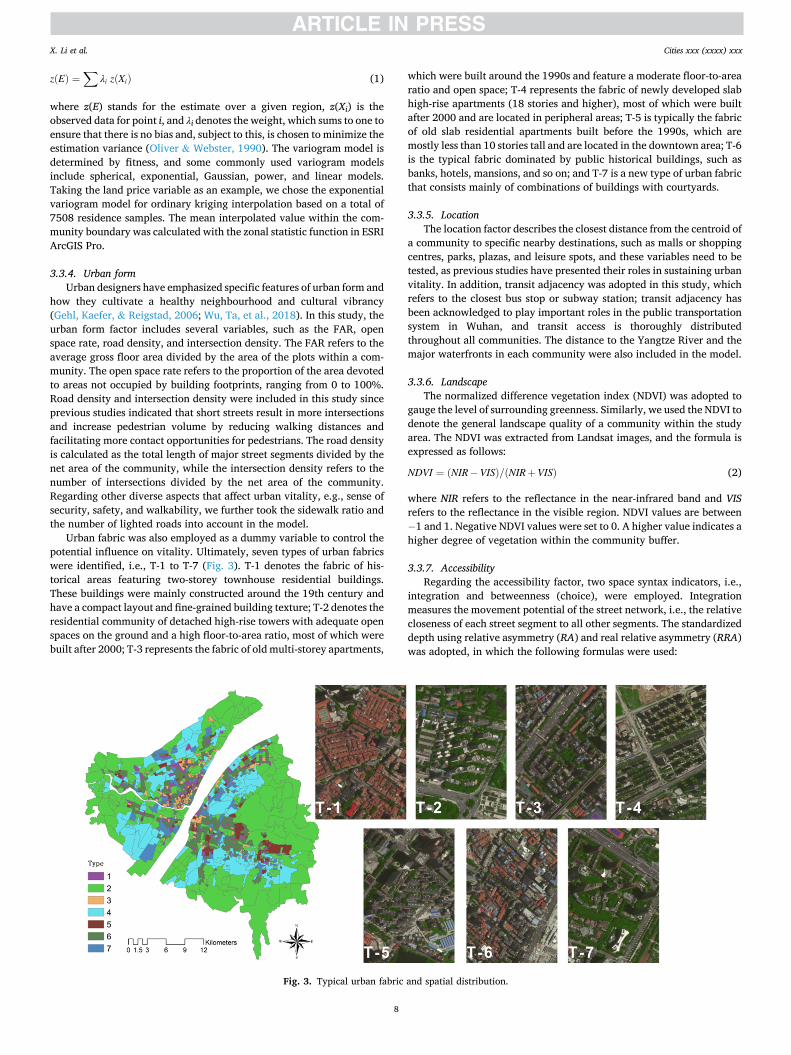
Urban fabric was also employed as a dummy variable to control the potential influence on vitality. Ultimately, seven types of urban fabrics were identified, i.e., T-1 to T-7 (Fig. 3). T-1 denotes the fabric of his-torical areas featuring two-storey townhouse residential buildings. These buildings were mainly constructed around the 19th century and have a compact layout and fine-grained building texture; T-2 denotes the residential community of detached high-rise towers with adequate open spaces on the ground and a high floor-to-area ratio, most of which were built after 2000; T-3 represents the fabric of old multi-storey apartments,

which were built around the 1990s and feature a moderate floor-to-area ratio and open space; T-4 represents the fabric of newly developed slab high-rise apartments (18 stories and higher), most of which were built after 2000 and are located in peripheral areas; T-5 is typically the fabric of old slab residential apartments built before the 1990s, which are mostly less than 10 stories tall and are located in the downtown area; T-6 is the typical fabric dominated by public historical buildings, such as banks, hotels, mansions, and so on; and T-7 is a new type of urban fabric that consists mainly of combinations of buildings with courtyards.

3.3.5. Location The location factor describes the closest distance from the centroid of

a community to specific nearby destinations, such as malls or shopping centres, parks, plazas, and leisure spots, and these variables need to be tested, as previous studies have presented their roles in sustaining urban vitality. In addition, transit adjacency was adopted in this study, which refers to the closest bus stop or subway station; transit adjacency has been acknowledged to play important roles in the public transportation system in Wuhan, and transit access is thoroughly distributed throughout all communities. The distance to the Yangtze River and the major waterfronts in each community were also included in the model.

3.3.6. Landscape The normalized difference vegetation index (NDVI) was adopted to

gauge the level of surrounding greenness. Similarly, we used the NDVI to denote the general landscape quality of a community within the study area. The NDVI was extracted from Landsat images, and the formula is expressed as follows:

NDVI = (NIR − VIS)/(NIR+VIS) (2)

where NIR refers to the reflectance in the near-infrared band and VIS refers to the reflectance in the visible region. NDVI values are between − 1 and 1. Negative NDVI values were set to 0. A higher value indicates a higher degree of vegetation within the community buffer.

3.3.7. Accessibility Regarding the accessibility factor, two space syntax indicators, i.e.,

integration and betweenness (choice), were employed. Integration measures the movement potential of the street network, i.e., the relative closeness of each street segment to all other segments. The standardized depth using relative asymmetry (RA) and real relative asymmetry (RRA) was adopted, in which the following formulas were used:

Fig. 3. Typical urban fabric and spatial distribution.

X. Li et al.

Cities xxx (xxxx) xxx

9

Integration = RA/RRA (3)

RA = 2(MD − 1)/n − 2 (4)

RRA = 2[n(log(n+ 2)/3 − 1 )+ 1 ]/(n − 1)(n − 2) (5)

where n is the number of units in the street network and MD is the average depth of segment i.

Betweenness is a measure of the penetration of a street network, i.e., the number of times a street segment is traversed as the shortest path from all origins to all destinations in the network (Hillier et al., 1987).

Betweenness =∑

j

∑

idjk(i)/djk (6)

where djk refers to the shortest path between segments j and k and djk(i) refers to the shortest path containing segment i between segments j and k.

Table 5 summarizes the statistics for all the variables adopted in this study.

3.4. Methods

To understand the spatial pattern of urban vitality, Moran's I was calculated; the value ranges from − 1 to 1, with the absolute value reflecting the degree of spatial autocorrelation. Then, local Moran's I was further calculated to identify different clusters with high-high values (HHs) and low-low values (LLs). Moreover, outlier clusters of high-low values (HLs) and low-high values (LHs) were also identified.

Since the community units are spatially interconnected, the focal community might be affected by its neighbouring communities,

violating the independence assumption of the traditional ordinary least squares (OLS) model. Therefore, a spatial lag multivariate regression model (SLM) was used to eliminate the bias of autocorrelation (LeSage & Fischer, 2008). For the SLM model, the lagged term of the dependent variable is considered to reduce the interference from neighbouring communities. The formula of the SLM is defined as follows:

Y = β0 + ρWY +∑

iβi Xi + ε (7)

where Y represents the dependent variable (urban vitality), Xi represents the explanatory variable i, β0 is the intercept, βi is the estimated coef-ficient of the explanatory variable, W is the spatial weight matrix, with ρ as the spatial autoregressive coefficient, and ε is the error term.

4. Results

4.1. Spatial pattern description

Spatial autocorrelation analysis was carried out using GeoDa version 1.6.7 software, in which a weight matrix was created using queen con-tinuity. The results show that Moran's I of urban vitality is highly posi-tive (0.491) at a significance level of p = 0.01 using 999 permutation tests, suggesting a spatial relationship at the community level. The Moran's I values of most BE variables are between 0.108 and 0.764, indicating a positive spatial autocorrelation at the significance level of p = 0.01, except for land use mix and betweenness, which have weakly positive spatial autocorrelations.

Fig. 4 depicts the spatial distribution of urban vitality and other selected BE variables in the study area. A strong spatial variation in urban vitality was observed, mainly overlapping with the highly

Table 5 Summary statistics.

Domains Variable Mean Std. Min Max Definition

Neighbourhood attributes (NE)

Population density (Pop)

3.822 3.557 0.007 39.987 Number of permanent residents per net area (100/ha)

Community age (Age) 18.347 3.908 0.000 27.544 Average building age in the community (year) Housing price (PR) 1.802 0.397 0.575 4.736 Average housing price per square meter within communities (10,000 Yuan/

m2) Urban form (FO) Floor-area ration (FAR) 1.088 0.802 0.000 7.645 Total square feet of building space of all kinds divided by the total square feet

within a plot Open space (OP) 85.041 11.281 0.000 100.000 Proportion of areas devoted to open spaces (%) Intersection (InS) 2.584 1.749 0.000 12.932 Number of intersections per net area (/ha) Road density (Rd) 176.352 77.735 0.000 571.249 Length of roads per net area (m/ha) Sidewalk percentage (SW)

1.603 2.354 0.013 30.667 The length of the sidewalk divided by the total length of roads (%)

Street lights (SL) 0.0000 1.000 − 0.909 7.304 Normalized value of the number of the street lights Facilities and land use

(FA) Food (FD) 2.696 3.763 0.000 47.545 Density of food facilities (/ha) Life service (SER) 3.362 4.368 0.000 51.589 Density of life service facilities (/ha) Shopping (SH) 5.510 9.675 0.000 134.605 Density of shopping facilities (/ha) Lodging (HOT) 0.454 1.299 0.000 27.661 Density of lodging facilities (/ha) Transit stops (Bus) 0.082 0.117 0.000 1.125 Density of bus-stop (/ha) Leisure (LEI) 0.396 0.582 0.000 6.190 Density of leisure and sport facilities (/ha) Tourist Attraction (AT) 0.047 0.155 0.000 1.840 Density of tourist attractions (/ha) Work place (WK) 1.268 2.102 0.000 17.429 Density of offices and institutions (/ha) Land use mix (LUM) 0.7113 0.321 0.000 1.000 Percentage of residential land use

Location (L) Distance to river (D.R) 2.390 2.453 0.000 13.961 Distance to the Yangtze River and other major waterfronts (km) Distance to commercial (D.Co)

0.249 0.362 0.000 3.541 Distance to the nearest mall or shopping center (km)

Distance to park (D.Pk) 0.693 0.548 0.000 4.039 Distance to the nearest park (km) Distance to bus-stop (D. Bus)

0.239 0.173 0.010 1.498 Distance to the nearest bus stop (km)

Distance to subway (D. Sub)

0.624 0.471 0.050 4.341 Distance to the nearest subway station (km)

Distance to leisure (D. Lei)

0.172 0.171 0.002 1.898 Distance to the nearest leisure or sport facility (km)

Distance to plaza (D.Pl) 0.867 0.515 0.009 3.547 Distance to the nearest plaza, square, or street garden (km) Landscape (LA) NDVI 16.968 5.071 4.509 46.182 Normalized degree of vegetation index (%) Accessibility (A) Integration (INT) 0.000 1.000 − 1.729 4.634 Normalized depth of street configuration

Betweeness (BT) 0.000 1.000 − 1.237 5.245 Normalized frequency of street segment traversed as the shortest path from all origins to all destinations in the network

X. Li et al.

Cities xxx (xxxx) xxx

10

Fig. 4. Spatial distribution of urban vitality and BE factors in Wuhan.

Fig. 5. Hotspots of urban vitality and several typical streetscapes.

X. Li et al.

Cities xxx (xxxx) xxx

11

integrated streets within a walkable distance (Fig. 6). There appears to be a much higher level of urban vitality on the northern bank of the Yangtze River, where the old downtown area of Hankou is situated, whereas the broad areas on the urban fringe are less active. Further-more, local Moran's I was applied to identify geographical clusters with statistically high or low urban vitality (Fig. 5), and the results confirmed that urban vitality was unevenly distributed at the community level. In Hankou, the largest agglomeration of communities with a high level of urban vitality occurs around the wholesale market area between Hanzheng Street and Youyi Road. The communities along Jinghan Avenue and Jiefang Avenue present a continuous accumulation. How-ever, the overall magnitude of urban vitality on the southern bank is much lower, with only several intermittent hotspots of moderate-level bifurcation along two directions from the old city centre. One direc-tion attenuates along the main corridor (Wuluo Road) to the east hin-terland, and the second direction extends along the Yangtze River water front to northern industrial compounds.

4.2. Regression models

As shown in Fig. 7, there were strong positive correlations among food, life services, and shopping facilities. Therefore, we adopted only the shopping facility for modelling to reduce multicollinearity. Although integration and betweenness also presented a strong positive correlation (Fig. 7), they were included in the model with variance inflation factor (VIF) values <5 for all adopted variables, which means that there was no serious multicollinearity problem. Six categories of BE factors, i.e., neighbourhood attributes, urban form, facility/land use, location, landscape, and accessibility, were included in the model in succession, and the results are shown for Model 1 to Model 6 (Table 6). For estimate optimization, a spatial regression model was further applied to reduce the bias of spatial autocorrelation. Based on a set of Lagrange multiplier tests (LM lag, LM error, robust LM lag, and robust LM error), the SLM model was eventually chosen because the robust LM error test is nonsignificant at the 95% confidence level. The results of these stepwise SLMs remained stable.

For Model 1, in which only the neighbourhood attribute factor was adopted, population density and community age presented a signifi-cantly positive association with urban vitality at the confidence level of p = 0.001, whereas the influence of land price was nonsignificant (p =0.802). When the urban form factor was added, as shown in Model 2, the FAR presented a significantly positive association with urban vitality (p = 0.033), while the road density influence was significantly negative (p < 0.001). According to the results, the sidewalk ratio and number of streetlights significantly promoted the level of urban vitality. Moreover, certain types of urban fabrics influence the differentiation of urban vi-tality. In Model 3, after the facility factor is adopted, three variables, i.e., shopping density, bus stop density, and leisure density, presented significantly positive associations with urban vitality, whereas nonsig-nificant influences were detected for other facilities (p > 0.1). The proportion of residential land had a significantly negative effect on urban vitality (p = 0.017). Notably, the influence of the FAR became nonsignificant when facility factors were added (p = 0.733). When the location factor was added to Model 4, urban vitality significantly decreased with a shorter distance to parks (p = 0.003). In contrast, shorter distances to bus stops (p = 0.001), subway stops (p = 0.003), and plazas (p = 0.022) significantly lead to a higher volume of urban vitality, as presented in Model 4, while nonsignificant influences are derived with regard to the distance to the Yangtze River (p = 0.559), shopping centres (p = 0.916) and leisure spots (p = 0.492). In Model 5 and Model 6, the landscape factor and accessibility factor were successively added, and the results were stable. In these two models, the NDVI had a significantly negative effect (p = 0.001) on urban vitality, and the in-fluence of integration was significantly positive (p = 0.022), whereas betweenness had a nonsignificant negative effect on urban vitality (p >0.1). The adjusted R-squared from Model 1 to Model 6 continued to

increase from 0.407 to 0.583 when the aforementioned factors were included in succession, indicating that these models were stably opti-mized with highly moderate performance and that the combination of the selected variables was reasonable. To confirm these results, two other goodness-of-fit metrics, i.e., the Akaike information criterion (AIC) and Bayesian information criterion (BIC), were adopted, each of which presented consistent conclusions. Instead of the R-squared value, the AIC and BIC are more suitable for the spatial regression model. A lower AIC or BIC value indicates better model performance. The AIC of the SLM model is only 1830.5, which is much lower than that of the ordinary least squares model (AIC = 1967.1), indicating a better goodness of fit. In addition, the detailed pairwise correlation for those variables with statistical significance can be seen in the scatter plot matrix (Fig. 8), in which we can divide the community samples on both sides of the Yangtze River to ensure acceptable variable distribution and sample representation (in the figure, the red dots are for the samples on the southern bank, and the blue dots are for samples on the northern bank).

In summary, the variables with significantly positive impacts on urban vitality include population density, community age, open space rate, sidewalk ratio, number of streetlights, shopping density, bus stop density, distance to parks, and integration, while some variables have significantly negative effects, such as road density, proportion of resi-dential land, distance to bus stops/subway stations/plazas, and the NDVI.

According to Model 6 (Table 6), the spatial lag term of urban vitality is significant at the level of p = 0.001, presenting a positive spillover effect on adjacent communities, indicating that the urban vitality of a local region spreads to nearby areas. Due to the occurrence of spillover effects, estimate decomposition was further carried out to identify the direct effects and indirect effects using the partial derivative method (Elhorst, 2010). The direct effect denotes the influence of explanatory variables of the focal community on urban vitality, while the indirect effect reflects the extent to which variables influence neighbouring communities (Table 7). Furthermore, we constructed an SLM by adopting accessibility factors (i.e., integration and betweenness) at in-cremental radii from 800 m, and the results were consistent until the analysis included radii that reached 1500 m, at which the best model fitness was derived on the basis of the AIC, BIC, and log likelihood. Notably, integration's influence on urban vitality became nonsignificant when the analysis include a radius of 2500 m, but eventually, it became significant again for global metrics.

4.3. GWR results

The variables that were significantly related to urban vitality in the SLM were selected to determine spatial heterogeneity with geographi-cally weighted regression (GWR), which resulted in a good model fit with an average adjusted R2 of 0.832 and an AIC of 11,288.183, indi-cating a very high explanatory power. The range of standardized re-siduals was [− 1.47, 3.22], approximately 99% of which was in the range of [− 2.5, 2.5], showing that GWR had good overall performance (Table 8). The local R2 values are between 0.66 and 0.90, confirming that the data can be fitted well by using the GWR model (Fig. 9).

5. Discussion

The results show that the six dimensions of BE factors are more or less correlated with urban vitality. Among the explanatory variables that had positive effects, the importance of adequate population density was confirmed to maintain the liveliness of a place, which is consistent with the findings of many previous studies (Jacobs-Crisioni, Rietveld, Koo-men, & Tranos, 2014; Sung & Lee, 2015) that have addressed the pos-itive relationship between the community population and walking activities. The accumulation of residents also promotes the survival of small businesses around these communities, providing more potential for people. However, we note that the population alone does not

X. Li et al.

Cities xxx (xxxx) xxx

12

Fig. 6. Variations in integration and betweenness at incremental radii.

X. Li et al.

Cities xxx (xxxx) xxx

13

spontaneously sustain a city quarter with vibrancy without a supportive environment, as confirmed by the results of this study, which revealed a negative association between the proportion of residential land and urban vitality. For instance, there are some areas in this case where it is quite rare to observe a high degree of vibrancy, particularly in mono-functional residential quarters, because of the mismatch between human and urban spaces. The inadequacy of major destinations and the lack of supportive amenities make them less likely for people to be involved in nonwork activities. The reduction in opportunities for people to enjoy commercial, social, cultural, and other urban life activities within a suitable distance lowers the vitality of a place (Boessen, Hipp, Butts, Nagle, & Smith, 2018). To revitalize a place, it is necessary to create opportunities for people to enjoy various daily life activities by providing convenience and services, particularly shopping, leisure, and transportation facilities.

This study reveals that the overall degree of vitality is higher in communities with a longer built history. This result reminds us of the important role of old buildings in nourishing a lively neighbourhood, as emphasized by Jacobs (1961). In another study conducted in South Korea, Sung and Lee (2015) also attribute the existence of old buildings

that contribute to promoting human engagement in urban spaces, indicating that residents in communities with a longer history are more likely to walk out for different purposes. These old communities contain collective memories that are often time based, eventually evolving as local culture, which is the foundation of city attractiveness and vibrancy because it brings uniqueness to urban spaces, evokes people's identity to a place, and in turn enhances the city's collective memories (Tchouka-leyska, 2016; Zukin & Braslow, 2011). Similar results were confirmed by other findings in this study. For instance, compared to historical resi-dential communities (T-1), newly developed high-rise communities (consistently for T-2 and T-4, as well as for T-7 in some certain cases) significantly inhibit the formation of community vibrancy, whereas the other three types of old communities, e.g., T3, T5, and T6, present nonsignificant differences. Therefore, when facing the increasing de-mand for an improved living environment, the target of urban renewal should avoid the oversimplified clearance of old buildings while encouraging more humanized strategies to ensure holistic improvement and rehabilitation of old areas. A contextual difference could be found when we refer to another case in the US (Deng & Ma, 2015), in which the average housing age presented a negative association with residential

Fig. 7. Correlation matrix of the tested variables (the values within the circle are nonsignificant).

X. Li et al.

Cities xxx (xxxx) xxx

14

vacancy, possibly due to a larger influence of social stratification on housing selection in different neighborhoods, where households with lower income tend to be in older communities where facilities and public infrastructure are lacking or are poorly maintained. Such a situ-ation not only makes property values drop but also lowers taxes used for public welfare, which results in the deterioration of community living conditions and a further exodus of affordable residents (Nassauer & Raskin, 2014). In the context of China, both cultural and social psy-chological factors need to be reconsidered, as residents prefer to live in relatively mature urban communities, most of which have a longer history and are situated in downtown areas with good accessibility and a rich supply of amenities, which echoes the aforementioned findings. For instance, this study showed significantly positive influences of shopping density and bus stop density on urban vitality, which can be interpreted

as residents select places that have convenient access to a variety of transportation and retail amenities. Similar results could be found in other Eastern Asian areas, such as in Seoul (Im & Choi, 2019).

In addition to neighbourhood attributes, configurational accessi-bility, particularly street network integration, also greatly contributes to urban vitality in the long term, while the effect of passing through is nonsignificant. According to the results, the influence of integration on urban vitality remains consistently significant within a 20-minute walking distance (approximately 1500 m). The results indicate that integration has a combinatory influence together with other BE factors that shape the pattern of urban vitality, and we manage to extract the corresponding independent effects at the community level. As a funda-mental mechanism, the configurational potential could exploited for advantages of urban function and land use over time, whether changes

Fig. 8. Scatter plot matrix of several key variables with statistical significance.

X. Li et al.

Cities xxx (xxxx) xxx

15

or adjustments are made by zoning or planning strategies over the long history of urban evolution.

With the call to return roads back to pedestrians, the demand for fine-grained blocks and high road density also increase. Many urban designers have emphasized the important role of small block sizes in promoting the friendliness of streetscapes. In China, a new neighbour-hood policy of ‘opening up gated residential communities’ was proposed a few years ago, aiming to break the barrier of the gated community and create some resonance (Wu, Ta, et al., 2018). However, our study does not predict an expected effect on increased urban vitality. The results show that the effect of the intersection density on urban vitality is nonsignificant, whereas a negative effect of the road density on urban vitality is detected. In this sense, a more in-depth understanding of the effects of these factors on urban vitality is needed. Although it has been recognized that small blocks with higher intersection densities are more likely to facilitate human interactions on streets (Jacobs, 1961), it should be noted that small blocks alone are not a solution for promoting vibrant urban life without the fulfilment of other supportive conditions, such as a sense of security and a friendly walking environment (Gan et al., 2021). For instance, increasing the sidewalk ratio and improving continuity are needed, as well as improving the lighting conditions of public open spaces. In addition, the results indicate that a higher pro-portion of open space helps induce human flow to nearby areas, which is consistent with the findings of previous studies (Koohsari et al., 2015). Particularly for areas with intensified development, more public open spaces, e.g., urban plazas, squares, and pocket gardens, should be pro-vided because of the better accessibility to nearby residents.

This study shows a negative correlation between the NDVI and urban

vitality and shows a decline in urban vitality for communities with shorter distances to parks, which is consistent with previous contentions (Mouratidis & Poortinga, 2020). This result also supported the findings of a case study of US cities, in which Deng and Ma (2015) indicated that the NDVI is negatively related to residential occupancy. Due to the rapid urban expansion seen in Wuhan, the large amount of investment has driven the excessive construction of real estate, which exceeds the actual demand. A limited number of residents choose to live in these newly developed communities, which feature low density, a single function, and a lack of public services. It is difficult for public activities to occur without a stable social network. As most large parks in Wuhan are located in urban fringe areas with low accessibility and population density, the number of residents is too limited for adequate human flows in nearby communities. For parks located in urban centres, dead-end space is easily created, which is referred to as the ‘border vacuum’ by Jacobs (1961). Therefore, it is helpful to control the negative effects on walkability and human flows by reasonable subdivision, particularly when vacuum-adjacent areas lack major destination or cross-use op-portunities. These findings demonstrate that the old development mode that encourages extensive urban sprawl should imperatively change (Sung & Lee, 2015). A comprehensive planning strategy is needed to modify the configuration of existing streets, enhance the connectivity of road networks, open community blocks, and optimize winding streets and cul-de-sacs. These results suggest that green spaces may inhibit the sense of vibrancy, which can be anticipated, particularly when people are diffused throughout large-scale, open-air spaces. As some previous studies have reported that proximity to parks is not correlated with residents' physical activities (Jilcott, Evenson, Laraia, & Ammerman,

Fig. 9. GWR results and the spatial pattern of the influences of the selected model estimates.

X. Li et al.

Citiesxxx(xxxx)xxx

16

Table 6 Results of the regression models.

Variable Model-1 Model-2 Model-3 Model-4 Model-5 Model-6

B S.E. p B S.E. p B S.E. p B S.E. p B S.E. p B S.E. p

Cons. − 0.781 0.144 <0.001*** − 1.187 0.330 <0.001*** − 0.341 0.362 0.346 − 0.014 0.369 0.970 0.414 0.373 0.266 0.289 0.372 0.437 N Pop 0.036 0.007 <0.001*** 0.034 0.008 <0.001*** 0.031 0.008 <0.001*** 0.032 0.008 <0.001*** 0.023 0.008 0.003*** 0.019 0.008 0.017**

Age 0.034 0.006 <0.001*** 0.038 0.007 <0.001*** 0.028 0.007 <0.001*** 0.025 0.007 <0.001*** 0.024 0.007 0.001*** 0.022 0.007 0.001*** PR 0.013 0.052 0.802 − 0.008 0.051 0.881 0.038 0.050 0.440 0.029 0.052 0.577 0.018 0.052 0.734 0.027 0.051 0.603

Fo FAR 0.085 0.040 0.033 0.014 0.041 0.733 0.016 0.040 0.701 0.021 0.040 0.599 0.021 0.040 0.591 OP 0.011 0.003 <0.001*** 0.009 0.003 0.002*** 0.009 0.003 0.002*** 0.011 0.003 <0.001*** 0.010 0.003 <0.001*** InS − 0.001 0.023 0.973 − 0.020 0.022 0.361 − 0.020 0.022 0.376 − 0.007 0.022 0.741 − 0.001 0.022 0.951 Rd − 0.003 0.001 <0.001*** − 0.003 0.001 <0.001*** − 0.004 0.001 <0.001*** − 0.004 0.001 <0.001*** − 0.004 0.001 <0.001*** SW 0.032 0.009 0.001 0.042 0.009 <0.001*** 0.033 0.009 <0.001*** 0.035 0.009 <0.001*** 0.036 0.009 <0.001*** SL 0.001 0.000 <0.001*** 0.001 0.000 <0.001*** 0.001 0.000 <0.001*** 0.001 0.000 <0.001*** 0.001 0.000 <0.001*** T-1 (ref.) T-2 − 0.439 0.093 <0.001*** − 0.303 0.090 0.001*** − 0.262 0.089 0.003*** − 0.282 0.088 0.001*** − 0.275 0.088 0.002*** T-3 0.124 0.095 0.193 0.178 0.091 0.050** 0.168 0.090 0.061* 0.133 0.089 0.133 0.122 0.088 0.169 T-4 − 0.324 0.099 0.001*** − 0.301 0.094 0.001*** − 0.280 0.094 0.003*** − 0.318 0.093 0.001*** − 0.310 0.092 0.001*** T-5 − 0.026 0.115 0.821 0.078 0.110 0.478 0.128 0.109 0.239 0.121 0.107 0.257 0.079 0.108 0.462 T-6 − 0.144 0.080 0.072* − 0.096 0.076 0.208 − 0.080 0.075 0.288 − 0.092 0.074 0.218 − 0.097 0.074 0.189 T-7 − 0.118 0.093 0.206 − 0.096 0.089 0.278 − 0.079 0.088 0.370 − 0.118 0.087 0.173 − 0.130 0.087 0.134

Fa SH 0.105 0.026 <0.001*** 0.093 0.027 <0.001*** 0.076 0.027 0.005*** 0.080 0.027 0.003 HOT 0.041 0.033 0.216 0.040 0.033 0.219 0.020 0.033 0.533 0.026 0.033 0.418 Bus 0.390 0.063 <0.001*** 0.298 0.065 <0.001*** 0.275 0.064 <0.001*** 0.252 0.065 <0.001*** LEI 0.077 0.041 0.060* 0.082 0.041 0.046** 0.078 0.040 0.053* 0.067 0.040 0.097* AT − 0.075 0.063 0.234 − 0.061 0.063 0.332 − 0.045 0.062 0.473 − 0.052 0.062 0.397 WK 0.032 0.027 0.232 0.032 0.026 0.228 0.008 0.026 0.752 0.008 0.026 0.748 LUM − 0.098 0.061 0.108 − 0.149 0.062 0.017** − 0.141 0.062 0.022** − 0.154 0.061 0.012**

Lo D.R − 0.005 0.008 0.559 − 0.007 0.008 0.380 − 0.005 0.008 0.509 D.Co 0.006 0.056 0.916 0.017 0.055 0.754 0.014 0.055 0.803 D.Pk 0.175 0.060 0.003*** 0.173 0.059 0.003*** 0.155 0.059 0.008*** D.Bus − 0.439 0.135 0.001*** − 0.454 0.133 0.001*** − 0.440 0.133 0.001*** D.Sub − 0.140 0.047 0.003*** − 0.130 0.046 0.005*** − 0.121 0.046 0.009*** D.Lei 0.099 0.144 0.492 0.012 0.143 0.932 0.036 0.143 0.801 D.Pl − 0.152 0.066 0.022** − 0.174 0.066 0.008*** − 0.158 0.065 0.016**

La NDVI − 0.027 0.005 <0.001*** − 0.025 0.005 <0.001*** A INT 0.075 0.033 0.022**

BT − 0.007 0.031 0.816 Rho 0.554 <0.001*** 0.567 <0.001*** 0.490 <0.001*** 0.464 <0.001*** 0.434 <0.001*** 0.429 <0.001***

Adj. R2 0.407 0.492 0.546 0.565 0.578 0.583 LogL − 1060.759 − 981.866 − 924.132 − 902.181 − 886.521 − 880.270 AIC 2133.500 1999.700 1898.300 1868.400 1839.000 1830.500 BIC 2163.112 2088.516 2032.614 2026.200 2011.851 2003.177

Note: T-1 to T-7 denote the dummy variables of urban fabric. * 0.1. ** 0.05. *** 0.01.

X. Li et al.

Citiesxxx(xxxx)xxx

17

Table 7 Decomposition of spatial effects.

Variable SLM (800 m) SLM (1000 m) SLM (1500 m) SLM (2500 m) SLM (global)

Direct p Indirect p Direct p Indirect p Direct p Indirect p Direct p Indirect p Direct p Indirect p

N Pop 0.020 0.009*** 0.014 0.016** 0.021 0.013** 0.015 0.017** 0.020 0.019** 0.014 0.023** 0.021 0.010*** 0.015 0.015** 0.023 0.006*** 0.016 0.001*** Age 0.027 0.001*** 0.019 0.001*** 0.027 0.001*** 0.019 0.001*** 0.026 0.001*** 0.018 0.001*** 0.026 0.001*** 0.018 0.001*** 0.027 0.001*** 0.019 0.001*** PR 0.010 0.837 0.007 0.837 0.009 0.885 0.006 0.887 0.011 0.858 0.007 0.866 0.006 0.900 0.004 0.909 0.004 0.938 0.003 0.945

Fo FAR 0.029 0.470 0.020 0.473 0.029 0.468 0.020 0.475 0.027 0.491 0.019 0.503 0.029 0.491 0.020 0.495 0.027 0.519 0.019 0.528 OP 0.010 0.001*** 0.007 0.001*** 0.010 0.001*** 0.007 0.002*** 0.010 0.001*** 0.007 0.002*** 0.010 0.001*** 0.007 0.003*** 0.010 0.001*** 0.007 0.002*** InS − 0.007 0.763 − 0.005 0.765 − 0.008 0.707 − 0.005 0.712 − 0.004 0.800 − 0.003 0.806 − 0.009 0.760 − 0.006 0.760 − 0.010 0.678 − 0.007 0.685 Rd − 0.004 0.001*** − 0.003 0.001*** − 0.004 0.001*** − 0.003 0.001*** − 0.004 0.001*** − 0.003 0.001*** − 0.004 0.001*** − 0.003 0.001*** − 0.004 0.001*** − 0.003 0.001*** SW 0.044 0.001*** 0.030 0.001*** 0.043 0.001*** 0.030 0.001*** 0.044 0.001*** 0.030 0.001*** 0.044 0.001*** 0.031 0.001*** 0.042 0.001*** 0.030 0.001*** SL 0.086 0.001*** 0.060 0.001*** 0.086 0.001*** 0.060 0.001*** 0.086 0.001*** 0.059 0.001*** 0.086 0.001*** 0.060 0.001*** 0.088 0.001*** 0.062 0.001*** T-1 (ref.) T-2 − 0.276 0.002*** − 0.191 0.006*** − 0.275 0.003*** − 0.190 0.006*** − 0.273 0.002*** − 0.187 0.005*** − 0.274 0.002*** − 0.191 0.005*** − 0.280 0.002*** − 0.198 0.004*** T-3 0.107 0.238 0.074 0.250 0.108 0.239 0.075 0.249 0.102 0.261 0.070 0.270 0.109 0.232 0.077 0.240 0.114 0.227 0.080 0.242 T-4 − 0.363 0.001*** − 0.251 0.001*** − 0.362 0.001*** − 0.250 0.001*** − 0.361 0.001*** − 0.247 0.001*** − 0.363 0.001*** − 0.254 0.001*** − 0.365 0.001*** − 0.257 0.001*** T-5 0.081 0.472 0.056 0.477 0.085 0.457 0.059 0.462 0.071 0.470 0.049 0.471 0.091 0.434 0.064 0.438 0.102 0.370 0.072 0.375 T-6 − 0.099 0.185 − 0.069 0.193 − 0.098 0.207 − 0.068 0.218 − 0.101 0.167 − 0.069 0.177 − 0.097 0.189 − 0.068 0.199 − 0.094 0.214 − 0.067 0.226 T-7 − 0.146 0.092* − 0.101 0.108 − 0.144 0.083* − 0.100 0.097* − 0.149 0.079* − 0.102 0.093* − 0.143 0.109 − 0.100 0.123 − 0.139 0.131 − 0.098 0.140

Fa SH 0.082 0.002*** 0.057 0.003*** 0.083 0.002*** 0.057 0.003*** 0.084 0.002*** 0.058 0.003*** 0.084 0.003*** 0.059 0.004*** 0.081 0.004*** 0.057 0.006*** HOT 0.020 0.538 0.014 0.545 0.019 0.511 0.013 0.518 0.020 0.556 0.014 0.567 0.015 0.680 0.010 0.687 0.019 0.586 0.013 0.588 Bus 0.241 0.001*** 0.166 0.002*** 0.237 0.001*** 0.164 0.001*** 0.237 0.001*** 0.162 0.001*** 0.240 0.001*** 0.168 0.001*** 0.249 0.001*** 0.175 0.001*** LEI 0.068 0.097 0.047 0.113 0.067 0.113 0.046 0.118 0.065 0.113 0.045 0.127 0.071 0.076* 0.050 0.088* 0.073 0.077* 0.051 0.089* AT − 0.058 0.344 − 0.040 0.354 − 0.056 0.372 − 0.039 0.377 − 0.055 0.380 − 0.038 0.390 − 0.048 0.403 − 0.034 0.403 − 0.047 0.493 − 0.033 0.497 WK 0.001 0.947 0.001 0.951 0.003 0.923 0.002 0.925 0.002 0.938 0.001 0.940 0.001 0.933 0.001 0.936 0.003 0.915 0.002 0.916 LUM − 0.157 0.011** − 0.108 0.017** − 0.157 0.011** − 0.108 0.017** − 0.159 0.012** − 0.109 0.018** − 0.154 0.016** − 0.108 0.021** − 0.153 0.017** − 0.108 0.021**

Lo D.R − 0.011 0.208 − 0.007 0.219 − 0.011 0.237 − 0.007 0.244 − 0.011 0.193 − 0.007 0.202 − 0.011 0.153 − 0.008 0.162 − 0.011 0.174 − 0.008 0.183 D.Co 0.031 0.530 0.022 0.528 0.033 0.582 0.023 0.584 0.034 0.574 0.023 0.574 0.034 0.512 0.024 0.512 0.030 0.609 0.021 0.610 D.Pk 0.214 0.001*** 0.148 0.002*** 0.215 0.001*** 0.149 0.002*** 0.210 0.001*** 0.144 0.002*** 0.217 0.001*** 0.152 0.001*** 0.224 0.001*** 0.158 0.001*** D.Bus − 0.451 0.001*** − 0.312 0.002*** − 0.452 0.001*** − 0.313 0.002*** − 0.452 0.001*** − 0.309 0.002*** − 0.457 0.001*** − 0.320 0.002*** − 0.458 0.001*** − 0.323 0.002*** D.Sub − 0.113 0.016** − 0.078 0.020** − 0.112 0.013** − 0.078 0.015** − 0.111 0.020** − 0.076 0.024** − 0.110 0.016** − 0.077 0.020** − 0.115 0.020** − 0.081 0.025** D.Lei 0.040 0.809 0.028 0.817 0.046 0.772 0.032 0.773 0.054 0.730 0.037 0.733 0.052 0.746 0.037 0.751 0.041 0.775 0.029 0.770 D.Pl − 0.209 0.003*** − 0.144 0.004*** − 0.209 0.003*** − 0.145 0.005*** − 0.204 0.003*** − 0.140 0.005*** − 0.210 0.001*** − 0.147 0.004*** − 0.214 0.002*** − 0.151 0.005***

La NDVI − 0.027 0.001*** − 0.019 0.001*** − 0.027 0.001*** − 0.019 0.001*** − 0.027 0.001*** − 0.018 0.001*** − 0.027 0.001*** − 0.019 0.001*** − 0.027 0.001*** − 0.019 0.001*** A INT 0.078 0.019** 0.054 0.022** 0.064 0.077* 0.044 0.084* 0.084 0.017** 0.058 0.019** 0.025 0.526 0.018 0.536 0.058 0.007*** 0.041 0.012**

BT − 0.008 0.789 − 0.005 0.804 0.012 0.738 0.008 0.739 0.002 0.965 0.001 0.954 0.047 0.207 0.033 0.219 − 0.010 0.643 − 0.007 0.642 Rho 0.429 0.001*** 0.430 0.001*** 0.427 <0.001*** 0.433 0.001*** 0.435 0.001*** LM-test 0.001 0.983 0.005 0.942 0.018 0.893 0.010 0.918 0.138 0.710 Adj. R2 0.583 0.583 0.585 0.583 0.581 Log-L − 880.270 − 887.590 − 877.934 − 880.408 − 882.735 AIC 1830.500 1829.600 1825.900 1830.800 1835.500

Note: T-1 to T-7 denote the dummy variables of urban fabric. * 0.1. ** 0.05. *** 0.01.

X. Li et al.

Cities xxx (xxxx) xxx

18

2007; McGinn, Evenson, Herring, Huston, & Rodriguez, 2007), it can even be argued that the lack of vitality and social interactions are some of the reasons why green spaces maintain calm nature and restorative-ness (Hartig, Mitchell, Vries, & Frumkin, 2014), and some of these places could be purposely preserved for a balanced development of humans and nature.

6. Conclusion and limitations

This study uses Wuhan, a typical megacity in China, to revisit the spatial pattern of urban vitality and influencing factors, which is an important subject of interest for the scientific community. By combining street movements with social media data, we developed a composite indicator as a surrogate of urban vitality. A rich variety of big data sources are combined to comprehensively clarify the BE vitality nexus while extracting the independent effects of street configuration on urban vitality. By systematically incorporating multidimensional BE factors, including neighbourhood attributes, urban form and function, land-scape, location, and street configuration, we adopt an advanced spatial regression model that resonates with traditional spatial syntax tech-niques to contribute to more in-depth understanding of the spatial dif-ferentiation of urban vitality in urban spaces as well as the driving force or inhibiting factors. This study enriches the existing literature by vali-dating previous theories and revealing additional potential associations between urban vitality and BE factors. The results show that population density, community age, open space, the sidewalk ratio, streetlights, shopping and leisure density, integration, and proximity to trans-portation are positive factors that induce urban vitality, whereas the effects of road density, proximity to parks, and green space have the opposite effect. The results of this comprehensive analysis contribute to an improved understanding of the BE vitality nexus, which helps mediate the relationship between planning policies and urban design strategies to optimize resource allocation and promote sustainable development. Based on the findings, both academic and managerial implications are discussed. To ensure the goodness of long-term sus-tainable development, the policy of optimizing the planning stock in urban China needs to be adhered to. The increasing demand for a better living environment should be in harmony with the renewal of existing urban spaces to ensure a holistic improvement of the city. According to the findings of our study, a high density facilitates vital and active communities based on the premise that some important conditions are met.

Some limitations of this study should be noted. First, although the fusion of street-view images with Weibo check-in data can reduce the temporal bias to some degree, it is still difficult to completely capture the temporal characteristics of urban vitality at a fine resolution. In

addition, the proxy of urban vitality is based on data captured from street-view images while some categories of activities may be more likely to be observed. In future studies, more data sources, e.g., mobile data, LBS data, and other social media data, could be added to further reduce this bias. Second, as this study is based on an empirical investi-gation in Wuhan, China, we must be cautious that possible controversies might occur in different contexts, for which additional research should be carried out to produce more generalized results. Moreover, additional investigations should be implemented to interpret the influence of spe-cific urban facilities with more detailed POI subcategories. How reliable estimates can be derived while satisfying multicollinearity standards will be further considered.

Funding sources

This work is supported by the National Natural Science Foundation of China (52078388, 41971332).

CRediT authorship contribution statement

Xin Li: Conceptualization; Methodology; Writing; Funding acquisition;

Yuan Li: Methodology; Data collection; Tao Jia: Project administration; Funding acquisition; Supervision; Lin Zhou: Software; Visualization; Data collection; Ihab Hijazi: Data analysis; literature review.

Declaration of competing interest

The authors declare that they have no known competing financial interests or personal relationships that could have appeared to influence the work reported in this paper.

References

Alalouch, C., Al-Hajri, S., Naser, A., & Al Hinai, A. (2019). The impact of space syntax spatial attributes on urban land use in Muscat: Implications for urban sustainability. Sustainable Cities and Society, 46.

Bakillah, M., Liang, S., Mobasheri, A., Arsanjani, J. J., & Zipf, A. (2014). Fine-resolution population mapping using OpenStreetMap points-of-interest. International Journal of Geographical Information Science, 28(9), 1940–1963.

Batty, M. (2010). The pulse of the city. Environment and Planning B: Planning and Design, 37(4), 575–577.

Batty, M. (2016). Empty buildings, shrinking cities and ghost towns. Environment & Planning B Planning & Design, 43(1), 3–6.

Boessen, A., Hipp, J. R., Butts, C. T., Nagle, N. N., & Smith, E. J. (2018). The built environment, spatial scale, and social networks: Do land uses matter for personal network structure? Environment And Planning B-Urban Analytics And City Science, 45 (3), 400–416.

Braun, L. M., & Malizia, E. (2015). Downtown vibrancy influences public health and safety outcomes in urban counties. Journal of Transport & Health, 2(4), 540–548.

Cao, X. Y., Mokhtarian, P. L., & Handy, S. L. (2009). Examining the impacts of residential self-selection on travel behaviour: A focus on empirical findings. Transport Reviews, 29(3), 359–395.

Carmona, M., & Sieh, L. (2004). Routledge. Cervero, R., & Duncan, M. (2003). Walking, bicycling, and urban landscapes: Evidence

from the San Francisco Bay area. American Journal of Public Health, 93(9), 1478–1483.

Chen, Z., Zhang, M., Cui, J., & He, S. (2015). Monitoring and modeling urban expansion—A spatially explicit and multi-scale perspective. Cities, 43, 92–103.

Conzen, M. R. G. (1960). London: George Philip. Deng, C., & Ma, J. (2015). Viewing urban decay from the sky: A multi-scale analysis of

residential vacancy in a shrinking U.S. city. Landscape & Urban Planning, 141, 88–99. Dhanani, A., Tarkhanyan, L., & Vaughan, L. (2017). Estimating pedestrian demand for

active transport evaluation and planning. Transportation Research Part A Policy & Practice, 103, 54–69.

Dizdaroglu, D. (2017). The role of indicator-based sustainability assessment in policy and the decision-making process: A review and outlook. Sustainability, 9(6).

Dovey, K., & Pafka, E. (2014). The urban density assemblage: modelling multiple measures. Urban Design International, 19(1), 66–76.

Elhorst, J. P. (2010). Applied spatial econometrics: Raising the Bar. Spatial Economic Analysis, 5(1), 9–28.

Ewing, R., & Clemente, O. (2013). Washington, DC: Island Press. Ewing, R., & Handy, S. (2009). Measuring the unmeasurable: Urban design qualities

related to walkability. Journal of Urban Design, 14(1), 65–84.

Table 8 Model estimates of GWR.

Variable Mean STD Min Median Max Model diagnosis

Intercept 0.131 0.267 − 0.351 0.075 0.801 R2 = 0.872 Pop 0.043 0.117 − 0.133 0.022 0.321 Adj. R2 = 0.832 Age 0.127 0.003 0.122 0.127 0.136 Log-L =

− 400.880 OP 0.022 0.003 0.013 0.022 0.027 AIC = 1288.183 Rd − 0.146 0.104 − 0.521 − 0.127 0.006 SW 0.314 0.345 − 0.322 0.227 1.523 SL 0.333 0.286 0.001 0.203 0.948 SH 0.129 0.002 0.125 0.128 0.134 Bus 0.005 0.003 − 0.003 0.006 0.012 LEI 0.032 0.075 − 0.113 0.037 0.251 LUM − 0.085 0.17 − 1.069 − 0.054 0.209 D.Pk 0.126 0.034 0.056 0.132 0.172 D.Bus − 0.118 0.076 − 0.39 − 0.106 0.017 D.Sub − 0.089 0.015 − 0.11 − 0.094 − 0.059 D.Pl − 0.082 0.003 − 0.09 − 0.083 − 0.077 NDVI − 0.085 0.001 − 0.087 − 0.085 − 0.084 INT 0.749 0.466 − 0.063 0.765 2.539

X. Li et al.

Cities xxx (xxxx) xxx

19

Filion, P., & Hammond, K. (2003). Neighbourhood land use and performance: The evolution of neighbourhood morphology over the 20th century. Environment & Planning B Planning & Design, 30(2), 271–296.

Foltete, J. C., & Piombini, A. (2007). Urban layout, landscape features and pedestrian usage. Landscape & Urban Planning, 81(3), 225–234.

Foster, S., Wood, L., Christian, H., Knuiman, M., & Giles-Corti, B. (2013). Planning safer suburbs: Do changes in the built environment influence residents' perceptions of crime risk? Social Science & Medicine, 97, 87–94.

Frank, L. D. (2000). Land use and transportation interaction: Implications on public health and quality of life. Journal of Planning Education & Research, 20(1), 6–22.

Gan, X., Huang, L., Wang, H., Mou, Y., Wang, D., & Hu, A. (2021). Optimal block size for improving urban vitality: An exploratory analysis with multiple vitality indicators. Journal of Urban Planning and Development., 147(3), 1–12.

Gavrilidis, A. A., Ciocanea, C. M., Nita, M. R., Onose, D. A., & Nastase, I. I. (2016). Urban landscape quality index - Planning tool for evaluating urban landscapes and improving the quality of life. Ecosmart - Environment at Crossroads: Smart Approaches for a Sustainable Development, 32, 155–167.

Gehl, J., Kaefer, L. J., & Reigstad, S. (2006). Close encounters with buildings. Urban Design International, 11(1), 29–47.

Gehl, J., & Svarre, B. (2013). How to study public life: Methods in urban design. Planning Perspectives, 29(4).

Grant, J. (2002). Mixed use in theory and practice: Canadian experience with implementing a planning principle. Journal of the American Planning Association, 68 (1), 71–84.

Hajrasouliha, A., & Yin, L. (2015). The impact of street network connectivity on pedestrian volume. Urban Studies, 52(13), 2483–2497.

Handy, S., Cao, X., & Mokhtarian, P. L. (2005). Correlation or causality between the built environment and travel behavior? Evidence from northern California. University of California Transportation Center Working Papers, 10(6), 427–444.

Hartig, T., Mitchell, R., Vries, S. D., & Frumkin, H. (2014). Nature and health. Annual Review of Public Health, 35(1), 207–228.

Hillier, B., & Hanson, J. (1984). Cambridge: Cambridge University Press. Hillier, B., Hanson, J., & Graham, H. (1987). Ideas are in things: An application of the

space syntax method to discovering house genotypes. Environment & Planning B Planning & Design, 14(4), 363–385.

Hillier, B., & Iida, S. (2005). Network effects and psychological effects: A theory of urban movement. In The proceeding paper of the fifth international symposium on space syntax (pp. 553–564). Delft.

Hillier, B., & Penn, A. (1996). Cities as movement economies. Urban Design International, 1(1), 49–60.

Hillier, B., Penn, A., Hanson, J., Grajewski, T., & Xu, J. (1993). Natural movement: Or, configuration and attraction in urban pedestrian movement. Environment & Planning B Planning & Design, 20(1), 29–66.

Hillier, B., Yang, T., & Turner, A. (2012). Normalizing least angle choice in depthmap and how it opens up new perspectives on the global and local analysis of city space. The Journal of Space Syntax, 3(2), 155–193.

Huang, H. S., Gartner, G., & Turdean, T. (2013). Social media data as a source for studying people's perception and knowledge of environments. Mitteilungen Der Osterreichischen Geographischen Gesellschaft, 155, 291–302.

Im, H. N., & Choi, C. G. (2019). The hidden side of the entropy-based land-use mix index: Clarifying the relationship between pedestrian volume and land-use mix. Urban Studies, 56(9), 1865–1881.

Jacobs, J. (1961). New York: Routledge. Jacobs-Crisioni, C., Rietveld, P., Koomen, E., & Tranos, E. (2014). Evaluating the impact

of land-use density and mix on spatiotemporal urban activity patterns: An exploratory study using mobile phone data. Environment And Planning a-Economy And Space, 46(11), 2769–2785.

Jiang, S., Alves, A., Rodrigues, F., Ferreira, J., Jr., & Pereira, F. C. (2015). Mining point- of-interest data from social networks for urban land use classification and disaggregation. Computers Environment & Urban Systems, 53, 36–46.

Jilcott, S., Evenson, K., Laraia, B., & Ammerman, A. (2007). Association between physical activity and proximity to physical activity resources among low-income, midlife women. Preventing Chronic Disease, 4(1), 1–16.

Jin, X., Long, Y., Sun, W., Lu, Y., Yang, X., & Tang, J. (2017). Evaluating cities' vitality and identifying ghost cities in China with emerging geographical data. Cities, 63, 98–109.

Karimi, K. (2012). A configurational approach to analytical urban design: 'Space syntax' methodology. Urban Design International, 17(4), 297–318.

Katz, P., Scully, V. J., & Bressi, T. W. (1994). New York: McGraw-Hill. Kim, H.-K., & Sohn, D. W. (2002). An analysis of the relationship between land use

density of office buildings and urban street configuration. Cities, 19(6), 409–418. Koning, R., Nes, A., Ye, Y., & Roald, H. (2017). Strategies for integrated densification

with urban qualities: Combining Space Syntax with building density, land usage, public transport and property rights in Bergen city. In Paper presented at the proceedingsof the 11th Space Syntax symposium.

Koohsari, M. J., Sugiyama, T., Sahlqvist, S., Mavoa, S., Hadgraft, N., & Owen, N. (2015). Neighborhood environmental attributes and adults' sedentary behaviors: Review and research agenda. Preventive Medicine, 77, 141–149.

Koster, H. R., & Rouwendal, J. (2012). The impact of mix land use on residential property values. Journal of Regional Science, 52(5), 733–761.

Krier, L. (2009). Washington: Island Press. Lamíquiz, P. J., & Lopez-Domínguez, J. (2015). Effects of built environment on walking

at the neighbourhood scale. a new role for street networks by modelling their configurational accessibility? - sciencedirect. Transportation Research Part A: Policy and Practice, 74, 148–163.

Lang, W., Chen, T., & Li, X. (2015). A new style of urbanization in China: Transformation of urban rural communities. Habitat International, 55(1), 1–9.

Lee, I. H., & Kim, Y. O. (2009). The effect of spatial configuration and land use pattern on land price formation. In Paper presented at the proceedings of the 7th international Space Syntax symposium, Stockholm, Sweeden.

Lerman, Y., Rofe, Y., & Omer, I. (2014). Using space syntax to model pedestrian movement in urban transportation planning. Geographical Analysis, 46(4), 392–410.

LeSage, J. P., & Fischer, M. M. (2008). Spatial growth regressions: Model specification, estimation and interpretation. Spatial Economic Analysis, 3(3), 275–304.

Li, M., Shen, Z., & Hao, X. (2016). Revealing the relationship between spatio-temporal distribution of population and urban function with social media data. GeoJournal, 81 (6), 919–935.

Li, Y., & Liu, X. (2018). How did urban polycentricity and dispersion affect economic productivity? A case study of 306 Chinese cities. Landscape and Urban Planning, 173, 51–59.

Liu, X. J., Sheng, Q., & Yang, Z. (2018). A feasibility study of streets view map on street quality evaluation. Urbanism and Architecture, 6, 40–43.

Liu, Y., Wei, X., Jiao, L., & Wang, H. (2016). Relationships between street centrality and land use intensity in Wuhan, China. Journal of Urban Planning & Development, 142(1), 1–14.

Lopes, M. N., & Camanho, A. S. (2013). Public green space use and consequences on urban vitality: An assessment of European cities. Social Indicators Research, 113(3), 751–767.

Lu, S. W., Huang, Y. P., Shi, C. Y., & Yang, X. P. (2019). Exploring the associations between urban form and neighborhood vibrancy: A case study of Chengdu, China. International Journal of Geo-Information, 8(4), 165. https://doi.org/10.3390/ ijgi8040165

Lu, X. H., & Ke, S. G. (2017). Evaluating the effectiveness of sustainable urban land use in China from the perspective of sustainable urbanization. Habitat International, 77, 90–98.

Lunecke, M., & Mora, R. (2018). The layered city: pedestrian networks in downtown santiago and their impact on urban vitality. Journal of Urban Design, 23(3), 336–353.

Lynch, K. (1984). Cambridge, MA, USA: MIT Press. Maas, P. R. (1984). Vancouver, BC, USA: University of British Columbia. Markusen, A. (2013). Fuzzy concepts, proxy data: Why indicators would not track

creative placemaking success. International Journal of Urban Sciences, 17(3), 291–303.

McCahill, C., & Garrick, N. W. (2008). The applicabilityof Space Syntax to bicycle facility planning. Transportation Research Record, (2074), 46–51.

McGinn, A. P., Evenson, K. R., Herring, A. H., Huston, S. L., & Rodriguez, D. A. (2007). Exploring associations between physical activity and perceived and objective measures of the built environment. Journal of Urban Health-Bulletin of the New York Academy of Medicine, 84(2), 162–184.

Montgomery, & John. (1998). Making a city: Urbanity, vitality and urban design. Journal of Urban Design, 3(1), 93–116.

Mouratidis, K., & Poortinga, W. (2020). Built environment, urban vitality and social cohesion: Do vibrant neighborhoods foster strong communities? Landscape and Urban Planning, 204.

Nassauer, J. I., & Raskin, J. (2014). Urban vacancy and land use legacies: A frontier for urban ecological research, design, and planning. Landscape and Urban Planning, 125, 245–253.

Oliver, M. A., & Webster, R. (1990). Kriging: A method of interpolation for geographical information systems. International Journal of Geographical Information System, 4(5), 313–332.

Omer, I., & Goldblatt, R. (2016). Spatial patterns of retail activity and street network structure in new and traditional Israeli cities. Urban Geography, 37(4), 629–649.

Ozbil, A., Peponis, J., & Stone, B. (2011). Understanding the link between street connectivity, land use and pedestrian flows. Urban Design International, 16(2), 125–141.

Porta, S., Latora, V., Wang, F., Rueda, S., Strano, E., Scellato, S., Cardillo, A., Belli, E., Cardenas, F., & Cormenzana, B. (2012). Street centrality and the location of economic activities in Barcelona. Urban Studies, 49(7), 1471–1488.

Shach-Pinsly, D. (2019). Measuring security in the built environment: Evaluating urban vulnerability in a human-scale urban form. Landscape and Urban Planning, 191.

Shach-Pinsly, D., & Ganor, T. (2021). A new approach for assessing secure and vulnerable areas in central urban neighborhoods based on social-groups' analysis. Sustainability, 13(3).

Shanahan, D. F., Lin, B. B., Gaston, K. J., Bush, R., & Fuller, R. A. (2015). What is the role of trees and remnant vegetation in attracting people to urban parks? Landscape Ecology, 30(1), 153–165.

Sheng, Q., Yang, T., & Hou, J. (2015). Continuous movement and hyper-link spatial mechanisms——A large-scale space syntax analysis on chongqing's vehicle and metro flow data. Journal of Human Settlements in West China, 30(5), 16–21.

Song, Y., Merlin, L., & Rodriguez, D. (2013). Comparing measures of urban land use mix. Computers Environment And Urban Systems, 42, 1–13.

Sternberg, & Ernest. (2000). An integrative theory of Urban Design. Journal of the American Planning Association, 66(3), 265–278.

Sung, H., & Lee, S. (2015). Residential built environment and walking activity: Empirical evidence of Jane Jacobs' urban vitality. Transportation Research Part D Transport & Environment, 41D(DEC.), 318–329.

Sung, H. G., Go, D. H., & Chang, G. C. (2013). Evidence of Jacobs's street life in the great Seoul city: Identifying the association of physical environment with walking activity on streets. Cities, 35, 164–173.

Tang, J. X., & Long, Y. (2019). Measuring visual quality of street space and its temporal variation: Methodology and its application in the Hutong area in Beijing. Landscape and Urban Planning, 191.

X. Li et al.

Cities xxx (xxxx) xxx

20

Tchoukaleyska, R. (2016). Public space and memories of migration: Erasing diversity through urban redevelopment in France. Social & Cultural Geography, 17(8), 1101–1119.

Tsou, K. W., & Cheng, H. T. (2013). The effect of multiple urban network structures on retail patterns - A case study in Taipei, Taiwan. Cities, 32, 13–23.

Vaughan, L., Jones, C. E., Griffiths, S., & Haklay, M. (2010). The spatial signature of suburban town centres. Journal of Space Syntax, 1(1), 77–91.

Wang, F., Chen, C., Xiu, C., & Zhang, P. (2014). Location analysis of retail stores in Changchun, China: A street centrality perspective. Cities, 41, 54–63.

Wang, F., & Guldmann, J. M. (1996). Simulating urban population density with a gravity- based model. Socio Economic Planning Sciences, 30(4), 245–256.

Weng, M., Ding, N., Li, J., Jin, X., Xiao, H., He, Z., & Su, S. (2019). The 15-minute walkable neighborhoods: Measurement, social inequalities and implications for building healthy communities in urban China. Journal of Transport & Health, 13, 259–273.

Whitehand, J. W. R., Samuels, I., & Conzen, M. P. (2009). Conzen, M.R.G. 1960: Alnwick, Northumberland: A study in town-plan analysis. Institute of British Geographers Publication 27. London: George Philip. Progress in Human Geography, 33(6), 859–864.

Wu, C., Ye, X., Ren, F., & Du, Q. (2018a). Check-in behaviour and spatio-temporal vibrancy: An exploratory analysis in Shenzhen, China. Cities, 77, 104–116.

Wu, J., Ta, N., Song, Y., Lin, J., & Chai, Y. (2018b). Urban form breeds neighborhood vibrancy: A case study using a GPS-based activity survey in suburban Beijing. Cities, 74(APR.), 100–108.

Xia, C., Yeh, A. G. O., & Zhang, A. Q. (2020). Analyzing spatial relationships between urban land use intensity and urban vitality at street block level: A case study of five Chinese megacities. Landscape and Urban Planning, 193.

Xiao, Y., Lu, Y., Guo, Y., & Yuan, Y. (2017). Estimating the willingness to pay for green space services in Shanghai: Implications for social equity in urban China. Urban Forestry & Urban Greening, 26, 95–103.

Yue, Y., Zhuang, Y., Yeh, A. G. O., & Xie, J.-Y. (2016). Measurements of POI-based mixed use and their relationships with neighbourhood vibrancy. International Journal of Geographical Information Science, 31, 658–675.

Yue, Y., Zhuang, Y., Yeh, A. G. O., Xie, J. Y., Ma, C. L., & Li, Q. Q. (2017). Measurements of POI-based mixed use and their relationships with neighbourhood vibrancy. International Journal of Geographical Information Science, 31(4), 658–675.

Zeng, C., Song, Y., He, Q., & Shen, F. (2018). Spatially explicit assessment on urban vitality: Case studies in Chicago and Wuhan. Sustainable Cities & Society, 296–306.

Zhang, H., Bian, J. M., & Wan, H. L. (2021). Hydrochemical appraisal of groundwater quality and pollution source analysis of oil field area: a case study in Daqing City, China. Environ. Sci. Pollut. Res., 28(15), 18667–18685.

Zhou, B., Zhao, H., Puig, X., Fidler, S., Barriuso, A., & Torralba, A. (2017). Scene parsing through ADE20K dataset. In Paper presented at the proceedings of the IEEE conference on computer vision and pattern recognition.

Zukin, S., & Braslow, L. (2011). The life cycle of New York's creative districts: Reflections on the unanticipated consequences of unplanned cultural zones. City Culture & Society, 2(3), 131–140.

X. Li et al.