The Romanian Economic Journal The Determinants of Corporate debt maturity: a study on listed...

The Romanian Economic Journal

Year XVII no. 51 March 2014

67

The study was intented to identify the determinants of the debt maturity structure of listed firms in Bombay Stock Exchange 500 index. For the analysis we have taken 321 firms during the period 2002- 2011, comprising of a panel model with fixed effects. We also used GMM (1991) and GMM (1998) estimates of our analysis. The result of robustness tests confirms that past year debt maturity, leverage and growth opportunities are directly determined the debt maturity of Indian firms. Liquidity, effective tax and rate prime lending rate are negatively determining the debt maturity of Indian companies. Keywords: debt maturity, panel data, GMM, Indian companies, fixed effect

JEL Classification: C23, G32

1 Raveesh Krishnankutty, Research scholar Faculty of Management Studies, ICFAI

University Tripura, India, [email protected] 2 Kiran Sankar Chakraborty, Regional Director, Indira Gandhi National Open University, Kolkata Regional Centre, Bikash Bhavan, Salt Lake, Kolkata-700091, India [email protected]

The Determinants of Corporate debt maturity: a

study on listed companies of Bombay Stock Exchange 500

index

Raveesh Krishnankutty1 Kiran Sankar Chakraborty2



68

1. Introduction

Mangers choose a debt maturity structure to maximize the value of the firm (Stephan et al., 2011). The maturity structure of debt capital is one of the vital elements of the capital structure decision. Debt capital has three major elements: duration (maturity period), fixed rate of interest and repayment of the principal. Cai et al. (2008) says firm might choose debt maturity policy to address agency problems. Furthermore, firms can signal the quality of their earnings by choosing a specific maturity mix. Moreover, the corporate debt maturity matters if firms happen to consider flexibility in financing, cost of financing, and refunding risk. Diamond and Rajan (2001) also emphasize its importance with reference to credit availability and financial crises.

The debt maturity structure has not yet received much attention in Indian context. Moreover, most of the existing studies of debt maturity structure predominantly focused on developing countries. To contribute to the existing literature in Indian context, this paper has been formulated. The objective of the study is to investigate the potential determinants of the debt maturity structure of Bombay Stock exchange (BSE) 500 index listed companies during the period 2002-2011.

The Bombay Stock exchange is the oldest, Asia largest stock exchange and world’s third biggest stock exchange in terms of volume of transactions. As India is the second biggest emerging economy after China and having a steady economic growth during the study period. However the Indian debt market still is not yet established as well as not getting much attention from the corporate sector. Banks are the major sources of debt capital for Indian companies. This would have a different implication on behalf of the rigorousness of agency theory, information



69

asymmetries, bankruptcy and taxation. Moreover, India is a mixed economy having number of government owned or controlling companies and private sector companies. Consequently, it is exciting to see the debt maturity theories were designed especially with respect to developed economies to the companies in the emerging economies.

Our empirical result reveals that leverage, growth opportunity and past year debt maturity positively determine the debt maturity, constant with predictions of maturity theories. Specified the estimated positive relation between maturity and growth opportunities, the paper reveals that the overinvestment problem has been paying more attention and is more discernible than the underinvestment problem. The findings, based on panel least squares with fixed effect weekly support the theories concerning growth opportunity, effective tax rate, etc. Nevertheless, after avoiding the indignity problem (the correlation between the error term and regressors) with the help of GMM (1991) and GMM (1998) methods, the expected positive sign for growth opportunity and negative sign of tax rate on debt maturity is found. However, negative sign liquidity is not providing a meaning full inference.

The reaming part of the paper is organized as follows. In Section 2 represent literature review. Section 3 describes research methodology, under methodology explaining variables used, sample, model, etc. In section 4 specified the empirical results and findings from different models. Section 5 compares the results of different models. Section 6 concludes the paper.

2. Literature review

Stephan et al. (2011) investigate the determinants of corporate debt maturity choice in emerging markets. Their estimates confirms that the importance of agency cost, liquidity, signalling and tax theories in a



70

transition economy for corporate debt maturity structure. They find that creditworthiness of the firm and access to long-term financing at bond market are the key drivers of corporate debt structure. Deesomask et al. (2009) examine the firm specific and country specific characteristics of the debt maturity structure of Asia pacific region. Their results indicate that firms in this region have a target optimal debt maturity structure. The maturity structure decision of a firm is driven by both its own characteristics and the economic environment. Cai et al. (2008) investigate the potential determinants debt maturity structure of Chinese listed firms. Their empirical analysis reveals that firm size, asset maturity and the liquidity factors tend to be significant in explaining debt maturity mix, consistent with predictions of maturity theories.

Kirch and Terra (2012) try to analyze, in a focus-country setting, how firm characteristics, quality of national institutions, and country level of financial development affect the debt maturity of firms from a sample of South American countries. They find that there is a substantial dynamic component in the determination of a firm's debt maturity, and firms face moderate adjustment frictions toward their optimal maturities. More importantly, the level of financial development does not influence debt maturity, whereas the institutional quality of a country has a significant positive effect on the level of long-term debt in a firm's financial structure. Their results also support the hypothesis that the quality of national institutions is an important determinant of corporate financing in general and of debt maturity in particular. Schmukler, and Vesperoni (2006) studies how financial globalization affects the debt structure in emerging economies. They find that by accessing international markets, firms increase their long-term debt and extend their debt maturity. In contrast, with financial liberalization, long-term debt decreases and the maturity structure shift to the short term for the average firm. These effects are stronger in economies with less developed domestic



71

financial systems. The evidence is consistent with financial integration having opposite effects on the firms that are able to integrate with world markets and obtain financing globally, relative to the firms that rely on domestic financing only. Aarstol (2000) proposes a new explanation for the inverse relationship between inflation and the maturity structure of business debt. It rests on the empirical finding that the variability of relative price changes increases with inflation. Qiuyan et al. (2012) employs the financial engineering approach to test the influencing factors of debt maturity structure with the data of 2012 listed companies distributed in 11 industries of China, by the simulation of single equation models and simultaneous equation model, using stepwise multiple regression analysis. The result of the paper conveys the endogenous relationship between capital structure and debt maturity structure matters a lot. Therefore, when the companies consider this relationship, the short-term debt maturity will not be an effective way to solve the problem of insufficient investment. In contrast, growth opportunity and leverage rate are significant negative correlation. With the role of leverage, growth opportunity will indirectly affect the debt maturity structure. Lopsz-Gracia and Mestre-Barbera (2011) analyses the influence of the tax effect on small and medium-sized (SME) enterprise debt maturity structure. This study builds a dynamic adjustment model which endogenous optimum structure and assumes the existence of adjustment costs. Using Spanish data, the model is estimated using a system- GMM regression to a complete panel 11,028 firms covering 1997–2004. The main results indicate that the model fits the data well and that SMEs seem to adopt an optimum debt maturity structure, which they converge to slowly due to the high adjustment costs they face. Average adjustment speed is estimated at around 37%, the equivalent of taking some 20 months to cover half the existing gap.



72

The effective tax rate is highly significant and both the interest rate gap and interest rate volatility also have a significant impact on debt maturity.

Hajiha and Akhlaghi (2012) test the main theories of firm debt maturity structure in an emerging economy, including agency conflict, signaling and tax theories. The paper investigates the firm specific determinants of debt maturity structure for a sample of 140 Iranian manufacturing firms listed on the Tehran Stock Exchange during the period 2001-2009. They have used random effect panel data analysis and multivariate regression for the analysis. The study provides the empirical evidence that profitability, firm size, tangibility, growth opportunity and financial leverage have significant effects on debt maturity choice . However, tax effects and business risk are not significantly related to the debt maturity structure.

3. Research Methodology

The debt maturity theories and their proxies for the study: The study considers the available debt maturity theories in order to constrain the dependent and independent variables in the analysis.

3.2 variables used for the study Dependent variables: in our study, the dependent variable are debt maturity, LTDTD. The ratio of long-term debt to total debt to measure debt maturity (Stephan et al. 2011, Cai et al. 2008, Antonious et al. 2006, Barclay and Smith. 1995). Independent variables: Antoniou et al. (2006) and Stohs and Mauer (1996), have divided the main debt maturity theories into four categories: agency costs, signaling and liquidity risks, matching and tax effect theories. Under each theory, we discuss the corresponding proxies and define their measurement to test the theories. Proxies for agency theory:



73

Growth opportunity: we measure the growth opportunity by using the variable GROWTH which is the sales growth to total asset growth. We assume that growth opportunity will be directly related to debt maturity. Firm size: We measure a firm's size (LNSA) by the natural logarithm of its total sales. We assume that debt maturity is directly related to firm size. .

Proxies for signaling and liquidity risk theories: Firm’s quality: Due to the lack data relating to the credit rating of the companies We measure firms’ quality as earnings before interest and tax to net sales (PROFIT). The study expects debt maturity to be inversely related to firms’ quality. Liquidity: We measure liquidity (CR) by current assets to current liabilities ratio (Myers and Rajan 1998, Morris 1992). The study predicts debt maturity will be directly related to liquidity. Leverage ratio: We measure leverage (TDTA) by the ratio of the book value of total debt divided by the book value of total assets. Morris (1992) Stohs and Mauer (1996) Leland and Toft (1996) Dennis et al. (2000). Debt maturity may be positively or inversely related to leverage as there is difference in findings of among literatures.

Proxies for matching principles: Asset maturity: Stohs and Mauer's (1996) was measured the asset maturity (NFADEP) by the sum of the weighted maturity of current assets and the weighted maturity of fixed assets. We calculate the un-weighted maturity of fixed assets by the ratio of net fixed assets to the depreciation (NFADEP), which shows the speed of consuming fixed assets. We expect that asset maturity will be positively related to debt maturity. Proxies tax theories:



74

Effective tax rate (EFTAX). We measure the effective tax rate (EFTAX) with the ratio of tax expense to pre-tax profit. Kane et al. (1985) indicate that the tax shield advantage is inversely related to debt maturity. In other words, if the effective tax rate is low, then firms prefer to issue long-term debt.Thus, we expect to find a negative relationship between debt maturity and the effective tax rate. We have used two macroeconomic variable to test its dependence on debt maturity. The proxies for macroeconomic variables are Prime lending rate (PLR): in India banks are the major contributor of debt capital. So we consider PLR will be an important factor that determine the debt maturity. We predict a negative relation between debt maturity and prime lending rate. Wholesale price index (WPI): wholesale price is having a major role in deciding the sales growths. It directly influences the company growth. So we predict a negative relation between WPI and debt maturity. 3.2 Data source The study is dealing with the Bombay Stock Exchange 500 index companies. The banking and finance companies are proposed to be kept out of the scope of the study. A period of ten years ranging from 2002 to 20011 is considered for the study. A total of 321 companies has been selected for the final analysis. Capital line data base is used for collecting the financial data for the prescribed period.

Table.1 Result of correlation analysis

LTDTD LNSA NFADEP TDTA GROWTH PROFIT EFTAX CR PLR WPI

LTDTD 1.00 -0.03 0.08 0.24 0.02 0.08 0.02 0.02 0.03 0.00

LNSA -0.03 1.00 -0.07 0.02 0.01 -0.09 -0.02 -0.18 0.03 0.33

NFADEP 0.08 -0.07 1.00 0.04 0.00 0.06 -0.01 0.00 0.00 -0.02



75

TDTA 0.24 0.02 0.04 1.00 0.02 -0.08 -0.01 -0.05 -0.01 -0.07

GROWTH 0.02 0.01 0.00 0.02 1.00 0.00 0.00 0.00 -0.02 -0.01

PROFIT 0.08 -0.09 0.06 -0.08 0.00 1.00 -0.01 0.14 0.05 0.08

EFTAX 0.02 -0.02 -0.01 -0.01 0.00 -0.01 1.00 0.00 0.02 0.00

CR 0.02 -0.18 0.00 -0.05 0.00 0.14 0.00 1.00 -0.01 0.00

PLR 0.03 0.03 0.00 -0.01 -0.02 0.05 0.02 -0.01 1.00 -0.14

WPI 0.00 0.33 -0.02 -0.07 -0.01 0.08 0.00 0.00 -0.14 1.00

The table. 1 shows the result of correlation analysis. The correlation among the independent variables is narrow. Same as the case for depended variable too.

3.3 Models

3.3.1 Panel least square with fixed and random effect

This study uses the balanced panel data for the analysis. Debt maturity is affected by so many other variable that are not included in this study such as the location of the firm managerial efficiency, marketing strategy, accounting policies, etc. the presence of these other variables may create inconsistent estimates so for minimizing the effects of these omitted variables the study is using firm specific control variables. There are two types of control variables: fixed effects and random effects. To decide between fixed or random effects we have to run a Hausman test where the null hypothesis is that the preferred model is random effects vs. the alternative the fixed effects (Green,

2008, chapter 9). It basically tests whether the unique errors ( ite ) are

correlated with the regressors; the null hypothesis is they are not.

Panel least square with fixed effect:



76

)1.(,.........)()()()()(

)()()()(

98765

4321

itititititit

ititititiit

eWPIPLRCREFTAXPROFIT

GROWTHTDTANFADEPLNSACFLTDTD

+++++++++++=

βββββββββα

Panel least square with Random effect

)2.(,.........)()()()()(

)()()()(

98765

4321

itititititit

ititititiit

eWPIPLRCREFTAXPROFIT

GROWTHTDTANFADEPLNSARELTDTD

+++++++++++=

βββββββββα

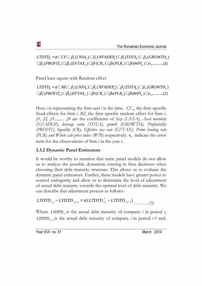
Here i is representing the firm and t is the time. CFi is the firm specific fixed effects for firm i. REi the firm specific random effect for firm i. β1, β2, β3.......... β9 are the coefficients of Size (LNSA), Asset maturity (NFADEP), leverage ratio (TDTA), growth (GROWTH), Profitability (PROFIT), liquidity (CR), Effective tax rate (EFTAX), Prime lending rate

(PLR) and Whole sale price index (WPI) respectively. ite indicate the error

term for the observations of firm i in the year t.

3.3.2 Dynamic Panel Estimators

It would be worthy to mention that static panel models do not allow us to analyze the possible dynamism existing in firm decisions when choosing their debt maturity structure. This allows us to evaluate the dynamic panel estimators. Further, these models have greater power to control endogenity and allow us to determine the level of adjustment of actual debt maturity towards the optimal level of debt maturity. We can describe that adjustment process as follows:

)( 1,*,1,, −− −=− titititi LTDTDLTDTDLTDTDLTDTD α

……….(3)

Where tiLTDTD , is the actual debt maturity of company i in period t,

1, −tiLTDTD is the actual debt maturity of company i in period t-1 and,



77

*,tiLTDTD is the optimal debt maturity of company i in period t.

Regrouping the terms and solving to the order of tiLTDTD , , we have:

))1( 1,*,, −−+= tititi LTDTDLTDTDLTDTD αα

………………(4)

If 1=α we have *,, titi LTDTDLTDTD α= , the actual level of debt maturity

being equal to the optimal level of debt maturity forcing firms to manage an optimal debt maturity structure. On the contrary, if, 0=αwe have 1,, −= titi LTDTDLTDTD i.e., there is no adjustment of the level of

actual debt maturity towards the optimal level of debt maturity. Therefore, a high values of α , means a close proximity of the level of actual debt maturity to optimal level of debt maturity, whereas a low values ofα , means less proximity between the actual level of debt maturity and optimal level of debt maturity.

It is important to mention that the optimal level of debt maturity depends on firms’ specific characteristics that are on the determinants considered relevant in explaining debt maturity as pointed out by Stephan et al. (2011), Cai et al. (2008) Therefore, the optimal level of debt is given by:

)5(,.........)()()()()(

)()()()(

98765

43210*,

itititititit

ititititti

uWPIPLRCREFTAXPROFIT

GROWTHTDTANFADEPLNSALTDTD

++++++++++=

λλλλλλλλλλ

Substituting (5) in (4), and solving to the order of tiLTDTD , , we have:

)6......(,.........)(

)()()()()(

)()()()(

9

87654

3211.0*,

itiit

ititititit

ititittiti

eWPI

PLRCREFTAXPROFITGROWTH

TDTANFADEPLNSALTDTDLTDTD

++++++++++++= −

ηβββββββββδβ



78

Where, )1( αδ −= , 00 αλβ = , 11 αλβ = , 22 αλβ = 33 αλβ = 44 αλβ = ,

55 αλβ = , 66 αλβ = , 77 αλβ = , 88 αλβ = , 99 αλβ = ii αµη = and itite αε= s

To control the correlation between iη and 1, −tiLTDTD between ite and

1, −tiLTDTD in estimating equation (6) using static panel models which

can give biased and inconsistent of the evaluated parameters, Arellano and Bond (1991) proposes evaluation of the equation (6) with the variables in first differences, and the use of debt lags and its determinants at level as instruments. However, Blundell and Bond (1998) concluded that when the dependent variable is persistent, there being a high correlation between its values in the current period and in the previous period, and the number of periods is not very high; the GMM (1991) estimator is inefficient; the instruments used will be generally being weak. In such cases by considering a system with variables at level and first differences Blundell and Bond (1998) extend the GMM (1991) estimator. For the variables at the level in equation (6), the instruments are the variables lagged in first differences. In the case of the variables in first differences in equation (6), the instruments are those lagged variables at level. However the GMM (1991) and GMM system (1998) dynamic estimators can only be considered robust on confirmation of two conditions: 1) if the restrictions created, a consequence of using the instruments, are valid; and 2) there is no second order autocorrelation. Therefore, to test the validity of the restrictions we use the Sargan test in the case of the GMM (1991) estimator and the GMM system (1998) estimator. The null hypothesis in the Sargan test indicates the restrictions imposed by the use of the instruments are valid against the alternative hypothesis that the restrictions are not valid. Rejection of the null hypothesis leads us to conclude that the estimators are not robust. Further, we also test for the existence of first and second order autocorrelation through Arellano and Bond (1991) test. The null hypothesis is that



79

there is no autocorrelation against the alternative hypothesis being the existence of autocorrelation. Rejection of the null hypothesis of the existence of second order autocorrelation leads us to conclude that the estimators are not robust.

4. Empirical results and findings

Table. 2 Result of panel least square with fixed effect

Variable Coefficient Std. Error t-Statistic Prob.

LNSA 0.05727 0.00705 8.12606 0.00000

NFADEP 0.00000 0.00009 0.05509 0.95610

TDTA 0.06885 0.01582 4.35282 0.00000

GROWTH 0.00001 0.00001 0.73365 0.46320

PROFIT 0.02287 0.01466 1.56034 0.11880

EFTAX 0.00238 0.00145 1.63696 0.10180

CR 0.00085 0.00020 4.18646 0.00000

PLR 0.00065 0.00248 0.26214 0.79320

WPI -0.00071 0.00014 -5.14910 0.00000

Constant 0.16306 0.04528 3.60109 0.00030

R-squared 0.613186 Adjusted R-squared 0.563455

F-statistic 12.33006*** Cross-section F- statistics 11.17798***

Note: ***, **, and *denote significance at 1, 5 and 10 percent level of significance respectively

The above table.2 show that the result of panel least square with fixed effect. The result of F- statistics shows that the model is fit and it is significant at one percent level. The values of R-square and Adjusted R-square are more than 0.5. It indicates that the independent variables could explain more than 50 percent variation in the depended variable. Significant Cross- section F-statistics indicates the presence of firm specific fixed effect in the model. The result of Firm size (LNSA) variable is consistent with the predicted sign. Moreover the result is in line with studies of Warner



80

(1977), Titman and Wessel (1988), Stephan et al. (2011), Cai et al. (2008). i.e., larger firms tend to issue long term debt Asset maturity (NFADEP) is having a positive sign, but statistically not significant. Leverage (TDTA) variable is positive and significant at the one percent level, confirms that high leverage firms tend use long- term debt .The result supports the studies such as Morris (1992), Stohs and Mauer (1996), Leland and Toft (1996). Growth opportunity (GROWTH), Firms quality (PROFIT), the effective tax (EFTAX) is showing a positive coefficient but insignificant. In case of Liquidity (CR) variable, the coefficient is positive and significant at the one percent level. The result indicates that a firm with more current assets, employs less long term debt in its capital structure. The macroeconomic variables employed in the study as the prime lending rate (PLR) is insignificant, wholesale price index (WPI) is negatively significant at the one percent level. It specifies that the proportion of long term debt in the total debt is lower at higher inflation. We could not show the result of panel least square with random effect because the result of cross-section test variance is invalid. Hausman statistic set to zero (see appendix). The below table.3 explains the result of dynamic panel data for the sample companies. From the results of the Sargan tests, we can conclude that we can reject the null hypothesis of instrument validity, and consequent restrictions generated, from use of the GMM (1991) and GMM system (1998) dynamic estimators respectively. However, the results of the second order autocorrelation tests concerning respectively the GMM (1991) and GMM system (1998) dynamic estimators, allow us to conclude that we cannot reject the null hypothesis of absence of second order autocorrelation. Therefore, given the validity of the absence of second order autocorrelation, but



81

instruments invalidity we cannot conclude that the GMM (1991) and GMM system (1998) dynamic estimators are efficient and robust.

Table.3 Result of dynamic panel least square

GMM 1991 GMM1998

Variables Coefficient Std. Er Prob. Coefficient Std. Er Prob.

L1.LTDTD 0.735 0.031 0.000 0.663 0.047 0.000

LNSA 0.021 0.013 0.094 0.028 0.015 0.063

NFADEP 5E-05 6E-05 0.45 5E-05 6E-05 0.446

TDTA 0.181 0.055 0.001 0.153 0.056 0.006

GROWTH 2E-05 0E+00 0.000 2E-05 0E+00 0.000

PROFIT -0.011 0.010 0.295 -0.010 0.011 0.344

EFTAX -3E-04 2E-04 0.089 -4E-04 2E-04 0.030

CR -2E-03 4E-04 0.000 -2E-03 5E-04 0.001

PLR -0.005 0.002 0.019 -0.005 0.002 0.030

WPI -2E-04 2E-04 0.355 -3E-04 2E-04 0.132

_CONS 0.015 0.074 0.844 0.048 0.078 0.534

Wald Chi 735.3*** 353.49***

Sargan test 42.85498 34.60435

AB Test Order 1 -8.4141*** -8.1737***

AB Test Order 2 1.1528 1.0667

Number of observations 2568 2247

Notes: 1. In the GMM(1991) estimator the instruments used are ),,(1

2,,2, ∑=

−−

n

Ktikti ZLTDTD in

which 2,, −tikZ are the debt maturity determinants lagged two periods. 2. In the GMM system

(1998) estimators the instruments used are ),,(1

2,,2, ∑=

−−

n

Ktikti ZLTDTD in the first difference

equations, and ),,(1

2,,2, ∑=

−− ∆∆n

Ktikti ZLTDTD in the level equations. 3. The Wald test has χ2



82

distribution and tests the null hypothesis of overall non-significance of the parameters of the explanatory variables, against the alternative hypothesis of overall significance of the parameters of the explanatory variables. 4. The Sargan test has χ2 distribution and tests the null hypothesis of significance of the validity of the instruments used, against the alternative hypothesis of non-validity of the instruments used. 5. The AB Test Order 1 test has normal distribution N(0,1) and tests the null hypothesis of absence of first order autocorrelation, against the alternative hypothesis of existence of first order autocorrelation. 6. The AB Test Order 2 test has normal distribution N(0,1) and tests the null hypothesis of absence of second order autocorrelation against the alternative hypothesis of existence of second order autocorrelation. 7. Standard deviations in brackets. 8. *** significant at 1% significance; ** significant at 5% significance; * significant at 10% significance.

The result shows that Last year debt maturity (L1.LTDTD) was positive and significant at the one percent level for both GMM (1991) and GMM (1998). It indicates that last year debt maturity had a positive influence in determining the current year debt maturity. The firm size (LNSA) variable has a positive and significant coefficient at 10% level for both GMM (1991) and GMM (1998). The result indicates small firms tend to be financed by short term debt. And larger firms will be tending to use long term debt to finance. The variable asset maturity (NFADEP) is insignificant using GMM (1991) and GMM (1998) also. It is contradictory to the studies such as Antoniou et al. (2006), Cai et al. (2008), Guedes and Opler. (1996). The leverage (TDTA) variable is showing a positive and significant coefficient at 10% level for GMM (1991) and at the one percent level for GMM (1998). I.e., the proportion of long term debt in the total debt will be higher in large firms.

Growth opportunity (GROWTH) variable has a positive significant coefficient at the one percent level for both GMM (1991) and GMM (1998). I.e., firm having high growth opportunity tends to put more long-term debt. It supports the over investment theory. The result is not supporting the Myers’ (1977) proposition that firms with high growth opportunity shorten the debt maturity. The variable Firm’s quality (PROFIT) has a negative insignificant coefficient for both the



83

models. The relationship between debt maturity and Effective tax (EFTAX) is negative at 10% level for GMM (1991) and at the five percent level. It indicates that the tax shield advantage is inversely related to issues of long term debt. In other words, in India the debt market is still under progress.

The variable liquidity (CR) has negative and significant coefficient at the one percent level for both GMM (1991) and (1998). The result is a bit contradictory with liquidity theories. Due to high operational cost and cut thought competition presents in Indian market a number of firms have tried to achieve under ideal current ratio. That may be the reason for negative sign. The macroeconomic variable Prime lending rate (PLR) is negatively significant at the 5 % level for both the GMM. It confirms that if firms will have more long term debt at low levels of rate of interest. Wholesale price index (WPI) has negative with insignificant coefficient.

GMM two-step standard errors are biased so we have done; robust standard errors have been checked. The result of the robustness test is shown in the below table.4.

Table.4 Result of Robustness test of Dynamic panel least square

GMM 1991 GMM1998

Variables Coefficient Std.

Error Prob. Coefficient Std.

Error Prob.

L1.LTDTD 0.735 0.043 0.000 0.663 0.058 0.000

LNSA 0.021 0.017 0.212 0.028 0.020 0.146

NFADEP 5E-05 5E-05 0.396 5E-05 5E-05 0.342

TDTA 0.181 0.065 0.006 0.153 0.064 0.016

GROWTH 2E-05 0E+00 0.000 2E-05 0E+00 0.000

PROFIT -0.011 0.009 0.242 -0.010 0.011 0.353

EFTAX -3E-04 2E-04 0.078 -4E-04 3E-04 0.122



84

CR -0.002 0.001 0.023 -0.002 0.001 0.080

PLR -0.005 0.003 0.042 -5E-03 3E-03 0.052

WPI -2E-04 2E-04 0.455 -3E-04 3E-04 0.201

_CONS 0.015 0.094 0.876 0.048 0.099 0.623

Wald Chi 377.26*** 212.91***

Sargan test 42.85498 34.60435

AB Test Order 1 -8.4141*** -8.1737***

AB Test Order 2 1.1528 1.0667

Number of observations 2568 2247

Notes: 1. In the GMM(1991) estimator the instruments used are ),,(1

2,,2, ∑=

−−

n

Ktikti ZLTDTD in

which 2,, −tikZ are the debt maturity determinants lagged two periods. 2. In the GMM system

(1998) estimators the instruments used are ),,(1

2,,2, ∑=

−−

n

Ktikti ZLTDTD in the first difference

equations, and ),,(1

2,,2, ∑=

−− ∆∆n

Ktikti ZLTDTD in the level equations. 3. The Wald test has χ2

distribution and tests the null hypothesis of overall non-significance of the parameters of the explanatory variables, against the alternative hypothesis of overall significance of the parameters of the explanatory variables. 4. The Sargan test has χ2 distribution and tests the null hypothesis of significance of the validity of the instruments used, against the alternative hypothesis of non-validity of the instruments used. 5. The AB Test Order 1 test has normal distribution N(0,1) and tests the null hypothesis of absence of first order autocorrelation, against the alternative hypothesis of existence of first order autocorrelation. 6. The AB Test Order 2 test has normal distribution N(0,1) and tests the null hypothesis of absence of second order autocorrelation against the alternative hypothesis of existence of second order autocorrelation. 7. Standard deviations in brackets. 8. *** significant at 1% significance; ** significant at 5% significance; * significant at 10% significance.

The above table.4 illustrates the result of robustness tests of dynamic panel least square. L1.LTDTD, TDTA and GROWTH have positively determined the debt maturity for both GMM. At the same time CR and PLR negatively determine the debt maturity for both GMM. In case of EFTAX it negatively determines debt maturity for GMM (1991) has a negative and insignificant coefficient for GMM (1998). The rest of the variables are not showing significance.



85

5. Comparison of results among models After comparing the result of different model used Leverage (TDTA) is positively significant in all the models. It confirms that large firms intend to have more long term debt. The variable firm size (LNSA) positively determines the debt maturity for panel least square fixed effect as well as GMM (1991) and GMM (19989). How even in case of robustness test it is having a positive insignificant coefficient. Growth opportunity (GROWTH), effective tax (EFTAX) and prime lending rate (PLR) are having an insignificant coefficient at panel least square fixed effect, other causes all the variables have significant coefficient. It indicates that in the panel it may be due to endogenity present in the fixed effect model. Liquidity (CR) variable is showing a positive sign in panel fixed effect model and the rest of the case it is negative. Wholesale price index (WPI) has a significant negative coefficient in case of panel fixed model remaining model it has a negative insignificant coefficient. This may be also due to the endogenity problem in the panel fixed effect model. Moreover GMM (1991) and GMM (1998) confirms that past year debt maturity (L1.LTDTD) is positively determining the current year debt maturity. Asset maturity (NFADEP) and Firm Quality (PROFIT) are insignificant in all cases. It may be that Indian debt marks are still not grown or underutilized. The firm mostly depended on banks for long term debt. And the long term debt is given on collateral security.

6. Conclusion The study was intended to identify the determinants of the debt maturity structure of listed firms in Bombay Stock Exchange 500 index. For the analysis we have taken 321 firms during the period 2002- 2011, comprising of a panel model with fixed effect. We also used GMM (1991) and GMM (1998) estimates of our analysis. The result of robustness tests confirms that past year debt maturity, leverage and growth opportunity directly determine the debt maturity



86

of Indian firms. It confirms that large companies will go for more long term debt in the total debt, i.e., it holds the liquidity theory. Moreover, firms having a high growth opportunity will also go for long term debt confirms the agency cost theory of overinvestment. Liquidity, effective tax and rate prime lending rate are negatively determining the debt maturity of Indian companies. The negative relationship between liquidity and debt maturity in the Indian context has to check further. It is not supporting the liquidity theories. Effective tax negatively determining debt maturity, it supports that in India the firms are not getting the tax shield advantage. Or it may be due to high transaction and issuance cost prevailing in the Indian debt mark. The prime lending rate is negatively related to debt maturity. It support that if the rate of interest is low companies will prefer more long term debt. As we observed in our data set the endogenity problem, so future research in this area should take into account the endogenity issues. Reference Aarstol, M.P. (2000),“Inflation and debt maturity”,The Quarterly Review of Economics and Finance, 40(4):139-153 Antoniou, A. Guney, Y. and Paudyal, K. (2006), “The determinants of debt maturity structure: evidence from France, Germanyand the UK”, European Financial Management, 12(2) 161–194 Arellano, M. and Bond S. (1991), “Some Tests of Specification for Panel Data: Monte Carlo Evidence and An Application to Employment Equations”, Review of Economic Studies, 58 (2): 277-297 Barclay, M.J. and Smith, C.W. (1995),“The maturity structure of corporate debt”, Journal of Finance, 50(2): 609–631



87

Blundell M., Bond S. (1998), ‘Initial Conditions and Moment Restrictions in Dynamic Panel data Models’, Journal of Econometrics, 87(1): 115-143. Cai, K. Fairchild.R. and Guney,Y. (2008), “Debt maturity structure of Chinese companies”, Pacific- Basin Finance, 16(3): 268-297 Diamond, D.W. and Rajan, R. (2001), “Banks, short term debt, and financial crises: theory, policy implications, and applications”, Proceedings of Carnegie Rochester Series on Public Policy, 54: 37–71 Deesomsak, R. Paudyal, K. and Pescetto, G. (2009), “Debt maturity structure and the 1997 Asian financial crises”, Journal of Multinational Financial Management, 19(1): 26-42 Dennis, S. Nandy, D. And Sharpe, I.G. (2000), “ The determinants of contract terms in bank revolving credit agreements”, Journal of Financial and Quantitative Analysis, 35(1): 87–110 Greene, W. H. (2008), “Econometric analysis” 6th ed., Upper Saddle River, NJ: Prentice Hall. Hajiha, Z. and Akhlaghi, H. A. (2012), “The determinants of debt maturity structure in Iranian firms”, World Applied Science Journal, 18(5): 624-632. Kane, A. Marcus, A.J. and McDonald, R.L. (1985), “ Debt policy and the rate of return premium to leverage”, Journal of Financial and Quantitative Analysis, 20(4): 479–499. Kirch, G. and Terra, P. R.S. (2012), “Determinants of corporate debt maturity in South America: Do institutional quality and financial development matter?”, Journal of Corporate Finance, 18(4): 980-993 Leland, H.E. and Toft, K.B. (1996),“Optimal capital structure, endogenous bankruptcy, and the term structure of credit spreads”, Journal of Finance, 51(3):987–1019 Lopsz-Gracia, j. and Mestre-Barbera, R. (2011),“Tax effect on Spanish SME optimum debt maturity structure” Journal of Business Research, 64(6): 649-655



88

Morris, J.R.(1992),“Factors Affecting the Maturity Structure of Corporate Debt”, Working paper. University of Colorado at Denver Myers, S.C. (1977), “Determinants of corporate borrowing”, Journal of Financial Economics, 5(2): 146–176 Myers, S.C. and Rajan, R.G. (1998),“The paradox of liquidity”, Quarterly Journal of Economics, 113(3): 733–771 Qiuyan, Z. Qian, Z. and Jingjing, G. (2012), “On debt maturity structure of listed companies in financial engineering”, Systems Engineering Procedia, 4(1): 61-67. Schmukler, S. L. and Vesperoni, E. (2006), “Financial globalization and maturity in emerging economies”, Journal of Development Economics, 79(1): 183-207. Stephan, A. Talavera, O. and Tsapin, A. (2011), “Corporate debt maturity choice in emerging financial markets”, The Quarterly Review of Economics and Finance, 51(4): 141-151 Stohs, M.H. and Mauer, D.C.(1996), “The determinants of corporate debt maturity structure”, Journal of Business, 69(3): 279–312 Titman, S., Wessels, R., 1988. The determinants of capital structure choice. Journal of Finance 43(1): 1–19



89

Appendix I

Table 5 Result of panel least square with random effect

Variable Coefficient Std. Error t-Statistic Prob.

LNSA 0.02938 0.00555 5.29072 0.00000

NFADEP 0.00007 0.00009 0.86588 0.38660

TDTA 0.09498 0.01523 6.23626 0.00000

SGGTA 0.00001 0.00001 0.88683 0.37520

PROFIT 0.03647 0.01430 2.55024 0.01080

EFTAX 0.00247 0.00144 1.70830 0.08770

CR 0.00065 0.00020 3.26151 0.00110

PLR 0.00273 0.00246 1.11112 0.26660

WPI -0.00032 0.00013 -2.56695 0.01030

C 0.22578 0.04541 4.97248 0.00000

R-squared 0.028222 Adjusted R-squared 0.025185

F-statistic 9.290236*** Cross-section F 5.997399 Note: Cross-section test variance is invalid. Hausman statistic set to zero

***, **, and *denote significance at 1, 5 and 10 percent level of significance respectively

Table.6 Cross-section random effects test comparisons

Variable Fixed Random Var(Diff.) Prob.

LNSA 0.0573 0.0294 0.0000 0.0000

NFADEP 0.0000 0.0001 0.0000 0.0007

TDTA 0.0689 0.0950 0.0000 0.0000

SGGTA 0.0000 0.0000 0.0000 0.1819

PROFIT 0.0229 0.0365 0.0000 0.0000

EFTAX 0.0024 0.0025 0.0000 0.5894

CR 0.0009 0.0006 0.0000 0.0000

PLR 0.0007 0.0027 0.0000 0.0000

WPI -0.0007 -0.0003 0.0000 0.0000



90

The Romanian Economic Journal The Determinants of Corporate debt maturity: a study on listed...

Documents

Transcript of The Romanian Economic Journal The Determinants of Corporate debt maturity: a study on listed...