1

The role of incidental variables of time in mood assessment

Robin M. Hogarth,1* Mariona Portell,2 & Anna Cuxart3

robin.hogarth@upf.edu

mariona.portell@uab.cat

anna.cuxart@upf.edu

1ICREA & Universitat Pompeu Fabra, Department of Economics and Business, Ramon Trias Fargas, 25-27, 08005 Barcelona, Spain. 2Universitat Autònoma de Barcelona, Department of Psychobiology and Methodology of Health Sciences, Campus de Bellaterra, s/n, 08193, Cerdanyola del Vallès, Spain. 3Universitat Pompeu Fabra, Department of Economics and Business, Ramon Trias Fargas 25-27, 08005 Barcelona, Spain. * This research has been supported by a grant from the Spanish Ministerio de Ciencia y Innovación (number ECO2009-09834).

2

ABSTRACT

Determining what influences mood is important for theories of emotion and research on

subjective well-being. We consider three sets of factors: activities in which people are

engaged; individual differences; and incidental variables that capture when mood is

measured, e.g., time-of-day. These three factors were investigated simultaneously in a study

involving 168 part-time students who each responded 30 times in an experience sampling

study conducted over 10 working days. Respondents assessed mood on a simple bipolar

scale – from 1 (very negative) to 10 (very positive). Activities had significant effects but,

with the possible exception of variability in the expression of mood, no systematic

individual differences were detected. Diurnal effects, similar to those already reported in

the literature, were found as was an overall “Friday effect.” However, these effects were

small. Lastly, the weather had little or no influence. We conclude that simple measures of

overall mood are not greatly affected by incidental variables.

Keywords: Affect; mood; experience sampling; diurnal effects; day-of-the-week; weather;

multilevel analysis.

JEL codes: C93; I00; I19; I131

Version: July 20, 2010

3

1. INTRODUCTION

Understanding variability in levels of mood and happiness in daily life is an important topic

that has attracted a significant scientific literature (see, e.g., Bradburn, 1969;

Csikszentmihayli, 1990; Strack, Argyle, & Schwartz, 1991; Diener & Seligman, 2004;

Kahneman, Krueger, Schkade, Schwartz, & Stone, 2004). It is possible to conceive of this

variability as being moderated by three classes of variables. First are the activities in which

people are involved and specific events that occur (see, e.g., Csikszentmihayli, 1990; Clark

& Watson, 1988; Kahneman et al., 2004). Second are variables that are specific to

individuals such as age, gender, culture, and personality (see, e.g., Diener, Oishi, & Lucas,

2003; Oishi, Diener, Choi, D.-W., Kim-Prieto, & Choi, T., 2007). And third are time-

related factors that are beyond individual control and which form the background against

which daily life is lived. We call this third class of variables incidental.

The purpose of the present paper is to explore – within the same investigation – the

role of three incidental variables on the expression of mood, specifically, time-of-day, day-

of-the-week, and the weather. That each might affect mood matches common intuition.

Moreover, there is already a growing literature that documents effects, albeit separately (see

below).

Our study is motivated by two important issues. The first is to further understanding

of the joint effects of different cyclical factors on mood. Are there regularities? On what do

these depend? How? Are some incidental variables more important than others? The

second has a more practical orientation relating to the measurement of social well-being (or

happiness). Does it matter when such judgments are elicited? Whereas it is well-known

that such assessments can be affected by factors such as question order (see, e.g., Strack,

4

Martin, & Schwartz, 1988) or the occurrence of major events (positive or negative), it is not

clear how they are affected by what we have called incidental variables. Moreover, not only

is it important to establish whether such variables have reliable influences on mood but also

their magnitude.

The data we analyze were originally collected in two studies that used the

Experience Sampling Method (ESM) (Hurlburt, 1997; Hektner, Schmidt, &

Csikszentmihayli, 2007) to study everyday perceptions of risk (Hogarth, Portell, & Cuxart,

2007; Hogarth, Portell, Cuxart, & Kolev, in press). However, an important feature of both

studies was that the first question respondents were asked when prompted at random

moments was an assessment of mood. Indeed, the first three questions of both studies were

identical across experimental treatments (the second and third questions asked what

participants were doing and whether the activity was personal or professional in nature).

Thus, since in the analyses reported here we only use the first three responses, it is

reasonable to aggregate the two sets of data (see also below).

Unlike much of the recent literature on mood, we used a single bipolar measure. We

simply asked respondents “How would you evaluate your emotional state right now?” on a

scale from 1 (very negative) to 10 (very positive). Whereas this “overall mood” question

does not distinguish between negative and positive moods (Watson & Tellegen, 1985;

Clark & Watson, 1988) nor different types of moods (see, e.g., Stone, Schwartz, J.,

Schwartz, N., Schkade, Krueger, & Kahneman, 2006), it does provide a simple overall

measure to which our respondents could relate easily in the context of the other questions

they were asked. In addition, we note that the use of single questions of “subjective well-

being” is quite common in many happiness surveys and has provided meaningful data (see,

5

e.g., Frey & Stutzer, 2002; Diener & Seligman, 2004).1 As such, answers to our question

can be thought of as summary measures of overall mood, possibly equivalent to a ratio of

positive to negative moods. Later in this paper, we detail steps we took to assess the

validity and reliability of our single mood measure.

We collected data on mood (as defined above) by having respondents complete

prepared response sheets when triggered by text messages sent to their cellular telephones

at random moments during their working days. In short, by using cellular telephones

(owned by our respondents), we implemented the ESM and collected random samples of

mood in everyday settings. In addition, we also gathered data on what respondents were

actually doing when asked by the ESM to answer questions. The innovative feature of our

data collection and analysis is the joint consideration of effects on mood due to the three

classes of variables discussed above, namely: activities, individual differences, and

incidental factors.

Our main results document the fact that judgments of mood are affected by the three

classes of incidental variables we considered and, of course, the activities in which people

are engaged. However, although these incidental factors are statistically significant in our

study, they are not very predictive of overall assessments of mood, that is, the effects are

small.

This paper is organized as follows. In the next section, we describe the study in

terms of the participants and procedures used for data collection. This is followed by a

review of literature on incidental factors in studies of mood that provides the motivation for

1 We note here that in our second study (Hogarth et al., in press) we also collected data on emotional reactions (Bradley & Lang, 1994), and thus can use these data to support the appropriateness of our mood measure (see Section 5 below).

6

the analyses and results that we present in the subsequent section. Next, we outline the

steps taken to establish the validity and reliability of our single mood measure. In a final

section, we discuss the implications of our findings.

2. THE STUDY

The data were collected in two phases. The first took place in February and May of 2005,

the second in October of 2006. Each phase involved a separate ESM study designed to

illuminate the perception of risks (Hogarth, et al., 2007; in press) but, as noted above, since

the first three questions were identical in both (see below), we have combined the two

datasets for the purpose of the present analysis (that only involves these three questions).

Participants

All participants were students recruited from the Universitat Autònoma de Barcelona. A

condition of their participation was that they had part-time jobs (defined by at least one

third of full working days). There were 168 participants in all – 74 in phase 1 and 94 in

phase 2. There were more women than men – 46 vs. 28 in phase 1, and 64 vs. 30 in phase

2. They ranged in age between 17 and 56 with a median of 22 in phase 1, and 19 in phase

2. Those participating in phase 1 were each paid 30 euros. In phase 2, the remuneration

was 35 euros. Participants were required to respond to the questions detailed below as well

as to some additional questions that are irrelevant to this analysis. In addition, they were

required to attend sessions before and after the study for instructions and debriefing (that

included some further questions).

7

Procedure

We sent text messages to participants between 8 am and 10 pm over a two-week period that

excluded week-ends, i.e., for 10 consecutive working days. Depending on their working

hours, some participants received their messages between 8 am and 3 pm and the others

between 3 pm and 10 pm (43 and 125 participants, respectively).2 To determine when

messages should be sent, we divided time into segments of 15 minutes and chose six

segments at random each day (three for each group of participants).

When they received a message, participants were required to note the date and time

and to answer a series of questions.3 The first three questions and types of scale used were:

1. How would you evaluate your emotional state right now? Scale from 1 (very

negative) to 10 (very positive)

2. What are you doing right now? Open-ended and subsequently referred to as ACT.

3. Is ACT professional or personal in nature? Binary response, coded (0/1)

There were up to five additional questions after this that varied by phase and

experimental conditions within phases (Hogarth et al., 2007; in press).

After completing the task, participants were thanked, debriefed, and paid in a post-

experimental session in which they also answered demographic and other questions. Phase

1 participants also completed Rotter’s (1966) Internal-External “Locus of Control”

questionnaire (IE).

2 The objective was to send participants messages during the part of the day in which they were mainly at work. 3 All questions were asked in Spanish.

8

3. THE ROLE OF INCIDENTAL FACTORS

Prior studies have specifically and directly investigated factors that we classify as

incidental. Of particular importance are the possible impacts of the timing of mood

questions which can be classified as being due to the time-of-day (diurnal), day-of-the-

week, or seasonal. However, since our data does not contain sufficient samples of seasonal

observations, we exclude the latter from consideration.4

Diurnal effects. Investigators have considered the existence of mood cycles for

several types of mood (not just positive and negative) using a variety of different methods

from simple rating methods to ESM to the more comprehensive Daily Reconstruction

Method (DRM) pioneered by Kahneman et al. (2004).

A priori, this is not a simple area of investigation in that “natural” biological cycles

might well be masked by factors such as the social organization of the day as well as

specific events (cf., Clark & Watson, 1988). Thus, in an especially interesting study where

a heterogeneous sample of 18 adults were kept in isolation over five days, Monk, Fookson,

Moline, and Pollak (1985) measured several moods and activities at frequent intervals.

Their measures of “happy” (or positive mood) and overall “wellbeing” showed inverted-U

patterns with the maxima being achieved some 4.1 hours after waking. “Sad” (or negative

mood) had no temporal pattern.

Wood and Magnello (1992) had several different groups of respondents (students

and non-students) assess moods and energy levels at different points in the day. Their

conclusions were, in brief, that positive mood had a diurnal effect but negative mood did

4 Seasonal effects of weather on moods and behavior have been documented (see, e.g., Smith, 1979; Harmatz, Well, Overtree, Kawamura, Rosal, & Ockene, 2000).

9

not. Second, moods with cycles reached their peaks between 10 a.m. and noon, and

although energy levels dipped after lunch, they rose late at night for students. Third, they

speculated that whereas positive moods might have a biological component, negative

moods might reflect environmental factors to a greater extent. In a related study of chronic

fatigue syndrome patients and a control group, Wood, Magnello, and Sharpe (1992) again

found that diurnal patterns of energy were highly correlated with positive mood and

reached their peaks between 10 a.m. and noon but measures of negative affect showed no

diurnal pattern.

Further evidence for the inverted-U shaped curve across the day for positive affect –

and yet no relation for negative affect – can be found in several other studies (Thayer,

1987; Clark, Watson, & Leeka, 1989; Watson, Wiese, Vaidya, & Tellegen, 1999; Murray,

Allen, & Trinder, 2002; Peeters, Berkhof, Delespaul, Rottenberg, & Nicolson, 2006).

Stone, Smyth, Pickering, and Schwartz (1996) made a detailed study of the moods

experienced by 94 employees of a large insurance company in New York. They collected

data every 15 minutes over the course of most of one day using a diary method. They found

that moods were quite influenced by specific activities or location that were correlated with

times in the day (such as commuting in early morning/late afternoon or lunch at noon), but

that nonetheless other diurnal cycles were not dependent on such factors (in particular,

“rushed,” “ sad,” and “tired”).

Stone et al. (2006) analyzed a large dataset involving responses by 909 working

women in Texas using the DRM (Kahneman et al., 2004). They were able to tabulate

changes in twelve moods (assessed by adjectives) across one working day and noted

several distinctive diurnal patterns. There were peaks for positive emotions at noon and in

10

the evening and peaks for negative emotions in mid-morning and mid-afternoon. Other

moods had V and inverted-U shaped patterns (“tired” and “competent,” respectively). The

advantage of the methodology used by Stone et al. (2006) was its ability to capture a large

amount of relevant data. However, this was limited to the activities of a single day and thus,

by itself, could not capture variation in factors such as the weather. Nonetheless, as the

authors themselves state:

With regard to the diurnal cycles observed in this sample of Texas women, not only were several findings based on smaller scale studies replicated, we detected diurnal rhythms that to our knowledge have not previously been reported. A consistent and strong bimodal pattern was found for positive and negative emotions. For the three positive adjectives, emotion levels during the work day had a peak at noon and a second peak starting at about 7 p.m. and the higher level lasted the rest of the evening. Conversely, peaks for the six negative adjectives were at about 10 a.m. and then at 4 or 5 p.m., although this pattern was relatively weak for some of the adjectives. One interpretation of this bipolarity is that the elevation of negative emotions was due to work and that lunchtime provided a respite from the demands of the work environment, reducing negative emotions (and increasing positive emotions)…. (Stone et al., 2006, p. 145). Finally, we note an interesting implication of diurnal mood fluctuations on

behavior. Kramer (2001) found that stock returns (resulting from trading) tend to be higher

in the morning than in the afternoon, a finding she attributed to people suffering more from

depression earlier rather than later in the day, i.e., negative mood is less in the afternoon

than in the morning.

Day-of-the-week effects. Most people are familiar with feelings of “blue Mondays”

and “happy Fridays” (TGIF) as markers of starting and ending the work week. However,

what evidence exists to support these notions?

Rossi and Rossi (1977) reported a study of daily moods of university students over a

40-day period. Using a measure of the ratio of the endorsements of positive to negative

mood adjectives, they found an increasing trend in mood from Monday through Friday with

11

a stronger slope for men (n=15) than women (n=67). They explain this gender effect by

noting that women’s daily moods are confounded by effects of menstrual cycles that do not

match days of the week. However, they also show that there are day-of-the-week effects for

women controlling for effects of menstrual cycles.

In a further study involving undergraduate students (39 females and 35 males) who

completed mood reports for 84 consecutive days, Larsen and Kasimatis (1990) found a

strong weekly pattern of data similar to that of Rossi and Rossi (1977). Moreover, they

detected a systematic personality difference in that extraverts exhibited more variability in

daily moods than introverts.

Replication of these effects with larger and more representative samples has,

however, not proven successful. For example, Stone, Hedges, Neale, and Satin (1985)

carried out several studies with substantial samples of married men. Their findings can be

summarized by stating that although their respondents believed that Mondays were “blue”

and Fridays “happy,” this was not the case when mood was actually measured on those

days. (At week-ends, however, positive mood was generally higher and negative mood

lower.) In a diary study involving 166 married couples over six weeks, Bolger, De Longis,

Kessler, and Schilling (1989) found no day-of-the-week effects. However, from their study

one might also infer that these could be perturbed by other more impactful events.

Weather conditions. Most people have an intuitive feeling that mood levels vary

with weather. However, both mood and weather conditions can be classified on several

dimensions and the empirical research does not present a clear picture.

Several studies clearly show effects of weather on human actions where it is

assumed that mood, as a reaction to changes in weather, affects behavior. For example,

12

Hirshleifer and Shumway (2003) showed that the amount of sunshine is significantly

correlated (positively) with stock returns. Moreover they documented this effect across 26

countries (national exchanges) from 1982 to 1997 thereby providing support for an earlier

study by Saunders (1993) in the US (see also Trombley, 1997).5 Further evidence has been

provided by Rind (1996) and Rind and Strohmetz, (2001) who documented how beliefs

concerning good weather increased tips given in restaurants. Finally, Simonsohn (2007)

reported that university admissions officers change the weights of their selection criteria

according to weather patterns. In the presence of cloud cover (i.e., lack of direct sunshine),

academic attributes of candidates are weighted more heavily.

There is, however, some evidence that sunshine has a direct affect on mood

(broadly defined). High levels of sunlight have been seen to increase self-reports of

happiness (Schwartz & Clore, 1983) and other similar effects on mood have been reported

by Cunningham (1979) and Parrott and Sabini (1990). On the other hand, when Schkade

and Kahneman (1998) investigated life satisfaction in large samples of students in two

regions in the US that differ in desirable weather (the Midwest and Southern California),

they found no differences. But, when respondents were asked to rate life satisfaction of a

similar other in the other region, Midwesterners gave higher ratings to Californians than

themselves, a difference that Schkade and Kahneman (1998) referred to as a focusing

illusion.

Studies conducted some time ago had relatively few observations (participants and

times of measurement) but produced some interesting results. Thus, K. M. Goldstein (1972)

5 Unfortunately, Hirshleifer and Shumway (2002) point out that trading using a sunshine strategy would not be profitable because it would require so many trades that the transaction costs of trading would not be compensated by the expected benefits.

13

reported that better mood was associated with high barometric pressure on some measures

but low on others. In addition, his results suggested that gender and being an external (on

Rotter’s 1966 IE scale) might mediate reactions between mood and weather. Looking at

these results a decade later, Sanders and Brizzolara (1982) conducted a study using a larger

sample and came to the overall conclusion that the effect of weather on mood is most

marked by levels of humidity (better moods beings associated with low humidity). This

result was replicated by Howarth and Hoffman (1984) who conducted a study relating

measures of ten mood variables to eight weather variables collected from 24 male

respondents over eleven days. Humidity, temperature, and hours of sunshine were found to

have the greatest effects on mood. However, humidity was the most significant “predictor”

(in a regression and canonical correlation analysis).

Recently, Denissen, Butalid, Penke, and van Aken (2008) conducted a

comprehensive online diary study (N=1,233) that examined possible effects of six weather

parameters (temperature, wind power, sunlight, precipitation, air pressure, and photoperiod)

on three measures of mood (positive affect, negative affect, and tiredness). Using multilevel

analysis they found no significant effects of daily weather on positive affect. There were

main effects of temperature, wind power and sunlight on negative affect, and sunlight also

affected tiredness. However, overall weather fluctuations accounted for very little variance

in people’s day-to-day mood. Interestingly, through their multilevel analysis Denissen et al.

(2008) reported individual effects but these could not be explained by either personality

(the Five Factor model) or gender.

In a study by Keller, Fredrickson, Ybarra, Côté, Johnson, Mikels, Conway, and

Wager (2005), no relation was found between weather and mood at different times of the

14

year except that pleasant weather (high temperature or barometric pressure) was related to

higher mood during the spring as time spent outdoors increased. In short, these

investigators posit a post-winter contrast effect due to time spent outdoors in more pleasant

conditions.

At one level, it might seem surprising that the literature does not demonstrate

“simpler” effects of weather on mood. However, as noted, both weather and mood are

multidimensional and, in addition to the fact that the studies reviewed used a variety of

different methodologies, there is also the fact the sampling of weather took place at

different moments in the year and in different geographical locations. Also, people who

have experienced different weather conditions across their lives might well react in

different ways. Clearly, future research will need to control for all these kinds of factors

and the work to date can only be suggestive.

Non-incidental factors. As noted above, the second and third questions asked our

respondents what they were doing when asked to assess their mood. Thus, we can also

investigate to what extent current activities impact mood. Three types of variables are of

interest: (1) the kind of tasks participants were performing (recall they were part-time

students questioned mainly while at work); (2) whether participants were doing something

that was effectively personal or professional in nature. The literature, for example, shows

that people involved in “desirable” events exhibit better moods than those who are not so

involved (David, Green, Martin, & Suls, 1997); and (3) whether they were doing

something on their own or in the company of one or more others (the latter has been shown

to be associated with better moods, Clark & Watson, 1988).

15

4. RESULTS

Response rates

From the 5,040 (= 168 x 10 x 3) messages sent, 5,022 were received (99.6%). For various

reasons, people might not receive text messages when they are sent (e.g., cell telephones

may have been turned off). We therefore checked the extent to which messages were

received when they were sent. For phase 1, participants reported receiving messages

between zero and 22 minutes after they were sent with an overall mean (median) of 3 (2)

minutes. For phase 2, the range was between zero and ten minutes after reception (overall

mean of one minute). We deem both response rates and reported times of receiving

messages satisfactory.

An overview

The design of our study involved data that can be thought of as being collected at two

levels. One of these levels – termed level 1 – is represented by participants’ responses to

the 30 occasions on which they received text messages (i.e., at the level of occasions). The

other – level 2 – is at that of the participants themselves (i.e., characteristics of the

participants that do not change across the 30 occasions). Thus, for example, it is of interest

to know whether, say, mood at the moment judgments are elicited (question 1) is associated

with what participants were doing (question 2) – i.e., at level 1 – and also whether such

judgments reflect differences between the participants in, say, gender – i.e., at level 2. As

such, our data can be efficiently modeled using the techniques of hierarchical linear models

(Byrk & Raudenbush, 2002; H. Goldstein, 1995; Longford, 1993).

(Insert Table 1 about here)

16

Table 1 presents the outcomes of the analysis of such a hierarchical model and

provides an overview of our findings. In fact, we show six models to demonstrate the

additional effects of different classes of variables.

Model 1 simply estimates the overall mean of mood without accounting for any

other factors and the residual variance at level 2 and at level 1 (between and within

individuals, respectively). The estimate for overall mood is 6.76 on a scale of from 1 ("very

negative") to 10 ("very positive"). The intraclass correlation is 0.20, meaning that 20% of

the total variance in mood is accounted for by individual differences. Model 2 shows a

statistically significant and fairly large increase in mood (0.46 points) of being involved in

personal as opposed to professional activities. In Model 3, significant effects of different

types of activities, and the extent to which they involve interaction with other people, are

estimated. Model 4 introduces diurnal effects. Model 5 adds those due to the days of the

week, and Model 6 captures the effects due to weather.

It is important to emphasize that Table 1 provides an overview of all of our data and

that all the models have been estimated assuming fixed effects. We have also estimated

models assuming random effects and, in our discussion of results for each class of variables

below, we comment on implications of different ways of analyzing the data.

Level-2/personal variables

There are two kinds of level-2 variables: methodological and personal. For the former, we

recall that the study was conducted in two phases and, within phases, participants answered

questions either mainly in the morning or in the afternoon. As shown in Table 1, the

dummy variable for phase 2 is not significant thereby implying that it is reasonable to

17

aggregate the data from both phases for analysis. Nor is there a main effect for responding

in the morning or the afternoon but this distinction does interact with level 1 variables as

we will explain further below.

No effects for gender are shown in Table 1 because there were none. As to possible

effects of personality, we did have measures of Rotter’s (1966) IE scale (“Locus of

Control”) for the 74 participants in phase 1. Interestingly, whereas the correlation between

IE scores and mean mood was not statistically significant (r = -0.16), the correlation

between IE scores and the standard deviation of mood was (r= 0.34, p = .003), and

especially for women (r = 0.42, p = .004). The interpretation is that variability in

expressions of mood is associated with more externally-oriented personalities (and

particularly for women). It is not clear how this squares with previous work on locus of

control (see, e.g., Blair et al., 1999; Klonowicz, 2001) but it is suggestive of some

systematic effects.

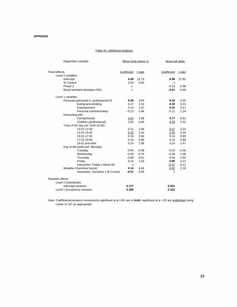
Table A1 in the Appendix shows the effect of including IE scores in a Model 6

analysis limited to phase 1 data. IE score has no main effect at level 2 but does interact

with weather (sunshine hours). Increased sunshine has a greater positive effect on the mood

of our more internally-oriented participants. We are unsure of the meaning of this

interaction. However, since IE score and the standard deviation of mood are correlated in

the phase 1 data, we created a proxy personality measure of variability in mood by using

the standard deviation of each participant’s mood measures. We included this as a level 2

variable in a re-analysis of Model 6. Although one might legitimately question this

statistical manipulation, the result – shown on the right hand side of Table A1 in the

Appendix – is that the standard deviation of mood has a significant negative relation with

18

mood at level 2 (coefficient = -0.61, t = -4.68, p< .001). In other words, variability in

expressions of mood is associated with lower levels of the same variable (cf., Beal &

Ghandour, 2010). Finally, there is also a significant interaction concerning the positive

effects of Fridays that are disproportionately greater if people exhibit less variability in

mood. We have no explanation for this interaction.

Activity effects

In our study, activities were reported by respondents in their own words in response to the

second question they received (i.e., after reporting mood). We classified these data as

follows. First, for data from phase 1 we established definitions of categories for the

activities. Then, two researchers independently allocated responses to categories (Kappa =

0.65). Disagreements between the two coders were resolved by having them discuss until

they reached consensus. Second, for data from phase 2, two coders were trained in the use

of the categories employed in phase 1. Then, they independently allocated responses to

categories and discussed disagreements with a third person (overall Kappa = 0.95). As a

third step, all the data for professional activities (phases 1 and 2) were submitted to an

additional analysis to determine more specific categories.

As will be no surprise to those familiar with the literature, our data show variation

in mood by the activities in which respondents were engaged (cf., Kahneman et al., 2004).

First, as shown by Model 2, being involved in personal as opposed to professional activities

has a positive impact (cf., David et al., 1997). Furthermore, several activities have

significant coefficients in Model 3 of Table 1 – in particular “Eating and drinking,”

“Entertainment,” and “Personal care/rest/sleep” – that are over and above the effect of the

19

dummy variable for “personal/professional.”6 In addition, there is a strong effect (0.81) for

interacting with family/friends (see also Clark & Watson, 1988). Further insight is

provided by Figure 1 that shows 95% confidence intervals of mean z-scores for mood

broken down by the categories of activities that we established and highlights the

distinction between personal and professional types of activity.7 These show that, relative to

each respondent’s average mood state, professional activities were generally associated

with negative (i.e., below average) mood whereas most personal activities were (with a

couple of exceptions) above average.

(Figures 1 through 3 about here)

A more detailed analysis of the Table 1 data broken down by whether participants

were working mornings or afternoons reveals an interaction with type of activity (not

shown in Table 1). Specifically, whereas the pattern of significant effects for different

activities for afternoon workers is the same as the whole sample, this is not true of morning

workers. For the latter, the coefficients for “Eating and Drinking” and “Entertainment” are

not statistically significant nor are the coefficients for interacting with “family/friends” and

“children”. On the other hand, the coefficient for “Personal care/rest/sleep” is significant (-

0.64, p <.001).8 A plausible interpretation of these results lies in the fact that the nature of

activities differed for participants in the morning and afternoon groups.

6 The reference category used as a base for coding the dummy variables for different activities was “Housework, personal time organization, and managing funds.” 7 We calculated z-scores for each individual respondent such that the mean of each person’s mood judgments is 0 with a standard deviation of 1. This allows us to categorize all observations/occasions as being positive or negative, i.e., whether they are above or below each individual’s mean mood score. 8 These results are robust to analyses assuming fixed or random coefficients.

20

Diurnal effects

Model 4 of Table 1 shows effects of time of day on mood relative to the period between 8

and 10:20 am. As can be seen, there are significant effects above this base level between

10:21 to 12:40 and 12.41 to 15:00. Thereafter, there is a significant effect at the end of the

day, i.e., from 19:41 and after. This pattern is illustrated in Figure 2 that shows 95%

confidence intervals for mood at different times of the day. As noted, mood starts low in the

morning, rises to the period between 12:41 to 15:00, and then falls sharply in the afternoon

before rising again in the evening.

Although this figure shows variations across the day, it is important to recall that the

data are comprised of morning and afternoon groups such that the three earlier estimates are

based predominantly on the morning group and the three later estimates on the afternoon

group. Nonetheless, the pattern of data is remarkably similar to results reported by other

researchers – for positive but not negative mood. (Reports of negative mood are that it is

almost “flat” or “unpredictable” across the day.) Several studies discussed in our review of

the literature provide evidence of a similar inverted-U pattern prior to the evening when

there is a late upturn (see, e.g., Monk et al., 1985; Wood & Magnello, 1992; Wood et al.,

1992; Peeters et al., 2006; Stone et al., 2006). One difference with our data, however, is

that the mid-day peak appears later than in the other, mainly US, studies. There is a

plausible cultural explanation. Whereas lunch usually starts at around 12 noon in the US, it

is much later in Spain, starting at 2 or even 3 pm. This external event appears then to

displace the diurnal pattern.

In short, we find a diurnal pattern in our data that is consistent with data from other

studies involving positive mood as well as energy levels. This suggests that our single

21

mood measure taps into either positive mood or the ratio of positive to negative mood

(since negative mood has been found to be flat across the day).

Day-of-the-week effects

Model 5 of Table 1 shows one day-of-the-week effect – a higher level of mood on Fridays.

This is also presented graphically in Figure 3. As noted in our review of literature, when

one excludes week-ends, effects for day-of-the-week are not a consistent finding although

our data do support the findings by Rossi and Rossi (1977) for a Friday effect in a student

population. Comparing the morning and afternoon groups, the patterns of day-of-the-week

effects are remarkably similar except that the Friday effect was marginally greater for the

morning group as compared with the afternoon group (not shown in Figure 3).

Weather conditions

We examined meteorological conditions for the dates when our data were collected and

identified 10 different measures.9 Of these, only one variable – daily sunshine (total

number of hours) – was statistically significant as shown by Model 6 of Table 1 (t = 2.13, p

< .05). However, when the same coefficient is estimated with robust standard errors, its

significance can be questioned (t = 1.56, p = .12). More importantly, whether statistically

significant or not, the effect is quite small.

9 These included: daily average temperature (ºC); precipitation (liter per square meter); rain (dummy variable,

1:yes; 0:not); daily sunshine (total number of hours); relative daily sunshine (percentage out of expected total hours); degree of cloudy at 7am (scale from 0 to 8); degree of cloudy at 1pm (scale from 0 to 8); daily solar radiation (watts per square meter); daily average of relative humidity (%); and daily average of barometric pressure(in hectoPascals, hPa). The data were obtained from the Servei Meteorològic de Catalunya , Xarxa d’Estacions Meteorològiques Automàtiques (XEMA) del Vallès Occidental and Observatori Fabra (Barcelona).

22

Overall then, our data do not show effects of variation in weather on mood. This

therefore adds to the confusion on this topic in the literature. One explanation for the lack

of effects in our data could be the nature of the generally pleasant Mediterranean climate

enjoyed in the Barcelona area. Although the data collection took place in different months,

February, May, and October, the latter two months are typically characterized by

comfortable weather and February is rarely very cold. If data collection had also taken

place in July and August, it is possible that discomfort from humidity could have been a

factor as reported in other studies (Sanders & Brizzolara, 1982; Howarth & Hoffman,

1984).

5. USING A SINGLE MEASURE OF MOOD

For a recent investigation of mood, our study is unusual in its use of a single measure. This

therefore calls for some justification. We present four arguments.

First, recall that we elicited self-reported mood in an ESM study where, to avoid

reactivity, we limited the number of questions (Hektner et al., 2007). The fact that only a

first, single question was used to elicit mood argues in its favor for dealing with one of the

more troubling issues in emotion research, namely, the need to synchronize the timing and

context of participants’ responses (Larsen & Fredrickson, 1999).

Second, we can ask whether the results we obtained with the measure have face

validity or, more precisely, what Hektner et al. (2007) refer to as situational validity. In

other words, are participants’ reports of mood coherent with other more “objective”

findings and data in the study? The answer is undoubtedly “Yes.” Consider, for example,

23

the findings reported above about better moods being associated with personal as opposed

to professional activities as well as the diurnal and day-of-the-week effects.

Our third argument is that we do, in fact, have some data for phase 2 of the study

that could be considered complementary to mood. Specifically, after completing the three

questions defined above (see Procedure), participants in this second phase were also

required to report feelings of their emotional states using the method of self-assessment

manikins (SAMs, Bradley & Lang, 1994). The SAMs represent visually three basic

dimensions of emotions in reactions to events or situations. These are (a) valence (or

pleasure), (b) arousal, and (c) dominance. Each emotion is captured by five “cartoon”

impressions, going from one extreme to the other. For example, valence is shown in the

form of five different figures (mainly faces) going from happy smiling to unhappy. For

each of the three emotions, participants simply checked the figure—or between adjacent

figures—that corresponded most to their feelings (thereby implicitly using nine-point

scales). Conceptually, one would expect valence to have some relation with our measure

of mood given that it taps into an intuitive sense of happiness. On the other hand, no

relation would be expected between mood and arousal although there might be a relation

with dominance (better mood being associated with more control).

(Insert Table 2 about here)

Table 2 reports correlations between our mood measure and the SAMs – both

between individuals (A) and within individuals (B). First note that there are appropriate and

significant correlations between mood and valence (happier valence being associated with

more positive mood). There is no significant relation between mood and arousal; and there

24

is a positive relation between mood and dominance (better mood, more dominance).

However, note that dominance and valence are also correlated in these data.

We realize, of course, that mood at a particular point in time is not the same thing as

emotional reactions to a situation. However, to the extent that these are simultaneous

expressions of affective states, we would expect coherence among different measures of

mood and emotions. Thus, the pattern of correlations in Table 2 supports the notion that our

mood measure has an appropriate level of reliability as well as demonstrating convergent

and discriminant validity.

Finally, our fourth point relates to a question the participants of phase 1 answered in

their post-experimental session. This was to assess their “emotional state over the last two

weeks” using the same 1 to 10 scale (“very negative” to “very positive”) as in the main

study. Whereas people’s memories of their past average mood states might be biased,

significant correlations between the stated average and estimates of actual experience

would provide further evidence of reliability of the mood scale. In fact, this correlation, i.e.,

between estimates of average mood over the two preceding weeks (the means of 30

judgments per individual) and participants’ remembered estimates, is 0.69 (n= 74, p<.001).

Parenthetically, this empirical result also speaks to the literature on the so-called

“peak-end” rule where it has been found that memory of the experience of sequential events

is better modeled by averaging the “peak” (i.e., most extreme) and “end” (i.e., last) stimulus

as opposed to the average of all stimuli experienced (see, e.g., Fredrickson & Kahneman,

1993). However, when we calculated the corresponding peak-end rule for our data, the

correlation with recalled experience was lower than for the mean (i.e., 0.35 vs. 0.69). There

are alternative explanations. One is that, for whatever reason, the peak-end rule result does

25

not apply to our data (see also, Kemp, Burt, & Furneaux, 2008). The second is that whereas

taking the mean of 30 randomly selected moments of experience provides an unbiased

estimate of average mood state, estimating the peak-end rule from our available data might

be biased. This is because there is no guarantee that the sequence of stimuli sampled

actually includes the most extreme experience (mood state) during the relevant period or,

indeed, the most recent mood state. Finally, we take heart from analytical results of

Cojuharenco and Ryvkin (2008) who showed that, under many conditions, peak-end and

average experience are quite highly correlated.

6. DISCUSSION

We used the experience sampling method to investigate assessments of mood made during

working hours by 168 part-time students on a simple bipolar scale – from 1 (very negative)

to 10 (very positive) – on 30 different occasions across a period of 10 working days. We

considered three classes of explanatory variables: types of activities; individual differences;

and incidental variables related to the times that measurements took place.

Participants also reported what they were doing on the occasions mood was

assessed and we used these self-report data to classify their activities. There was a strong

effect if the participants considered that their activities were personal as opposed to

professional in nature (personal activities being rated on average almost one-half point

higher on the mood scale). Moreover, if personal activities involved eating and drinking,

entertainment, or interaction with friends and family, assessments were even higher. These

effects are similar to other studies that have looked at everyday activities (e.g., Clark &

26

Watson, 1988; Kahneman et al., 2004).10 We also analyzed our data to look for possible

effects in the types of part-time work being done by our participants but, with the exception

of a small positive effect for those involved in professional childcare (i.e., babysitting), we

found no differences. A disadvantage of our methodology, of course, is that is ill-suited to

capturing possible systematic effects of unusual events or activities that occurred rarely.

With the exception of gender, our participants were quite homogeneous with respect

to age and other demographic characteristics typical of a part-time student population. As

such, one would not expect to find many effects due to individual differences. Moreover,

except for Rotter’s (1966) IE (“locus of control”) scores for 74 of the 168 participants, we

had no measures of personality. Nonetheless, two points were highlighted by our analysis.

First, there were no main effects for gender or even interactions involving gender. Second,

whereas IE scores did not correlate with mood, they did correlate with variability in mood

with more externally oriented participants having larger standard deviations of mood

scores. Building on this finding, we used standard deviations of mood as a proxy measure

of individual difference (i.e., for variability in mood) and identified an inverse relation

between levels of mood and variability across our whole sample. Whereas only suggestive,

this result highlights the potential importance of individual variability (Beal & Ghandour,

2010).

We investigated three types of incidental variables: diurnal, day-of-the-week, and

weather. Moreover, an important advantage or our methodology was that we could

estimate the potential effects of all from the same data. Our results are largely consistent

with findings in the literature.

10 We do not consider that the types of part-time work in which our respondents were engaged would have allowed for the type of “flow” experiences described by Csikszentmihayli (1990).

27

First, the diurnal pattern of our data suggests an inverted-U shape from morning

until the early evening followed by a rise in the later evening – see Figure 2. Such patterns

have also been observed in other studies that have examined feelings of positive mood

(e.g., Stone et al., 2006). Moreover, since negative mood appears to be unrelated to time

across the day, the argument can be made that total mood (as either the sum or ratio of

positive and negative mood) should also follow pattern that we observed. Finally, we note

that some studies have identified diurnal mood levels (and energy) to differ by age of

participants with older people starting high (in the morning) and ending low at night and

younger people having the reverse pattern (see, e.g., Wood & Magnello, 1992). The pattern

of data of our young, part-time student population clearly followed that of younger people.

Second, we identified a Friday effect – see Figure 3. As pointed out above, this is

both consistent (Rossi & Rossi, 1977) and inconsistent (Stone et al., 1985) with previous

findings of day-of-the-week effects.

Third, we essentially found little or no effects due to the weather. This is consistent

with recent findings concerning positive affect in the extensive, recent study by Denissen et

al., 2008). However, we are acutely aware that our sample of Mediterranean weather may

not have provided sufficient variation for effects to have been observed. Specifically, our

review of the literature suggested two variables that might be particularly relevant to mood

changes, namely; hours of sunshine, and humidity.11 We are intrigued by the possibility

that weather-related mood changes might interact with individual differences in a way that

needs to be specified in future research (cf., K. Goldstein, 1972).

11 In fact, our data suggest a small, “questionable” effect due to hours of sunshine.

28

Finally, whereas our analyses did identify some statistically reliable effects of

incidental variables on assessments of mood, it is important to emphasize that the effects

we found were not large in the sense that their incorporation would make much difference

in a predictive model. Often such a statement might be considered the “death knell” of a

scientific investigation. However, we do not believe that to be the case here. As stated at

the beginning of this paper, not only is it important to establish that effects exist (to

confront theories and intuitions), but sizes of effect are also important from a practical

perspective. For example, from the viewpoint of research on subjective well-being, it is

essential to establish the boundary conditions under which assessments of happiness are

and are not subject to systematic influences. Thus it is important to know that the main

effects of incidental effects are small. Whether their interactions with other variables – and

especially individual differences – are small provides another and open set of questions for

future research.

29

REFERENCES

Beal, D. J., & Ghandour, L. (2010). Stability, change, and the stability of change in daily

workplace affect. Houston, Rice University working paper.

Blair, A. J., Leakey, P. N., Rust, S. R., Shaw, S., Benison, D., & Sandler, D. A. (1999).

Locus of control and mood following myocardial infarction. Coronary Health Care,

3, 140-144.

Bolger, N., De Longis, A., Kessler, R. C., & Schilling, E. A. (1989). Effects of daily stress

on negative mood. Journal of Personality and Social Psychology, 57(5), 808-818.

Bradburn, N. M. (1969). The structure of psychological well-being. Chicago, IL:Aldine.

Bradley, M. M., & Lang, P. J. (1994). Measuring emotion: The self-assessment manikin

and the semantic differential. Journal of Behavioral Therapy and Experiential

Psychiatry, 25, 49-59.

Byrk, A. S., & Raudenbush, S. W. (2002). Hierarchical linear models: Applications and

data analysis methods. (2nd ed.). Newbury Park: Sage Publications.

Clark, L. A., & Watson, D. (1988). Mood and the mundane: Relations between daily life

events and self-reported mood. Journal of Personality and Social Psychology,

54(2), 296-308.

Clark, L. A., Watson, D., & Leeka, J. (1988). Diurnal variation in the positive affects.

Motivation and Emotion, 13(3), 205-234.

Cojuharenco, I., & Ryvkin, D. (2008). Peak-End rule versus average utility: How utility

aggregation affects evaluation of experiences. Journal of Mathematical Psychology,

52, 326-335.

Csikszentmihayli, M. (1990). Flow: The psychology of optimal experience. New York, NY:

HarperCollins.

Cunningham, M. R. (1979). Weather, mood, and helping behavior: Quasi experiments with

the sunshine Samaratin. Journal of Personality and Social Psychology, 37(11),

1947-1956.

David, J. P., Green, P. J., Martin, R., & Suls, J. (1997). Differential roles of neuroticism,

extraversion, and event desirability for mood in daily life: An integrative model of

30

top-down and bottom-up influences. Journal of Personality and Social Psychology,

73(1), 149-159.

Denissen, J. J. A., Butalid, L., Penke, L., & van Aken, M. A. G. (2008). The effects of

weather on daily mood: A multilevel approach. Emotion, 8(5), 662-667.

Diener, E., Oishi, S., & Lucas, R. E. (2003). Personality, culture, and subjective well-being:

Emotional and cognitive evaluations of life. Annual Review of Psychology, 54, 403-

425.

Diener, E., & Seligman, M. E. P. (2004). Beyond money: Towards an economy of well-

being. Psychological Science in the Public Interest, 5(1), 1-31.

Frederickson, B., & Kahneman, D. (1993). Duration neglect in retrospective evaluations of

affective episodes. Journal of Personality and Social Psychology, 65, 45-55.

Frey, B.S., & Stutzer, A. (2002). What can economists learn from happiness research?

Journal of Economic Literature, 40, 402-435.

Goldstein, H. (1995). Multilevel statistical models. (2nd ed.). Kendall’s Library of Statistics

3. London, UK: Edward Arnold.

Goldstein, K. M. (1972). Weather, mood, and internal-external control. Perceptual and

Motor Skills, 35, 786.

Harmatz, M. G., Well, A.D., Overtree, C. E., Kawamura, K.Y., Rosal, M., & Ockene, I.S.

(2000). Seasonal variation of depression and other moods: A longitudinal approach.

Journal of Biological Rhythms, 15, 344-350.

Hektner, J. M., Schmidt, J. A., & Csikszentmihayli, M. (2007). Experience sampling method:

Measuring the quality of everyday life. Thousand Oaks, CA: Sage Publications.

Hirshleifer, D., & Shumway, T. (2003). Good day sunshine: Stock returns and the weather.

Journal of Finance, 58(3), 1009-1032.

Hogarth, R. M., Portell, M., & Cuxart, A. (2007). What risks do people perceive in

everyday life? A perspective gained from the experience sampling method (ESM).

Risk Analysis, 27(6), 1427-1439.

Hogarth, R. M., Portell, M., Cuxart, A., & Kolev, G. I. (in press). Emotion and reason in

everyday risk perception. Journal of Behavioral Decision Making.

Howarth, E., & Hoffman, M. S. (1984). A multidimensional approach to the relationship

between mood and weather. British Journal of Psychology, 75, 15-23.

31

Hurlburt, R. T. (1997). Randomly sampling thinking in the natural environment. Journal of

Consulting and Clinical Psychology, 67 (6), 941-949.

Kahneman, D., Krueger, A, B., Schkade, D. A., Schwartz, N., & Stone, A. A. (2004). A

survey method of characterizing daily life experience: The day reconstruction

method. Science, 306 (5702), 1776-1780.

Keller, M. C., Fredrickson, B. L., Ybarra, O., Côté, S., Johnson, K., Mikels, J., Conway, A.,

& Wager, T. (2005). A warm heart and a clear head: The contingent effects of

weather in mood and cognition. Psychological Science, 16(9), 724-731.

Kemp, S., Burt, C. D. B., & Furneaux, L. (2008). A test of the peak-end rule with extended

autobiographical events. Memory & Cognition, 36 (1), 132-138.

Klonowicz, T. (2001). Discontented people: Reactivity and locus of control as determinants

of subjective well-being. European Journal of Personality, 15, 29-47.

Kramer, L. A. (2001). Intraday stock returns, time-varying risk premia, and diurnal mood

variation. Working paper, Department of Economics, Simon Fraser University.

Larsen, R. J. & Fredrickson, B. L. (1999). Measurement issues in emotion research. In D.

Kahneman, E. Diener & N. Schwarz (Eds.) Well-being: Foundations of hedonic

psychology (pp. 40-60). New York, NY: Russell Sage.

Larsen, R.J., & Kasimatis. M. (1990). Individual differences in entrainment of mood to the

weekly calendar. Journal of Personality and Social Psychology, 58(1), 164-171.

Longford, N.T. (1993). Random coefficient models. Oxford, UK: Oxford University Press.

Monk, T., Fookson, J., Moline, M., & Pollak, C. (1985). Diurnal variation in mood and

performance in a time-isolated environment. Chronobiology International, 2(3),

185–193.

Murray, G., Allen, N. B., & Trinder, J. (2002). Mood and the circadian system:

Investigation of a circadian component in positive affect. Chronobiology

International, 19(6), 1151-1169.

Oishi, S., Diener, E., Choi, D.-W., Kim-Prieto, C., & Choi, I. (2007). The dynamics of

daily events and well-being across cultures: When less is more. Journal of

Personality and Social Psychology, 93(4), 685-698.

32

Parrott, W. G., & Sabini, J. (1990). Mood and memory under natural conditions: Evidence

for mood incongruent recall. Journal of Personality and Social Psychology, 59(2),

321-336.

Peeters, F., Berkhof, J., Delespaul, P., Rottenberg, J., & Nicolson, N.A. (2006). Diurnal

mood variation in major depressive disorder. Emotion, 6(3), 383-391.

Rind, B. (1966). Effects of beliefs about weather conditions on tipping. Journal of Applied

Social Psychology, 26(2),137-147.

Rind, B., & Strohmetz, D. (2001). Effects of belief about future weather conditions on

restaurant tipping. Journal of Applied Social Psychology, 31(10), 2160-2164.

Rossi, A. S., & Rossi, P. E. (1977). Body time and social time: Mood patterns by menstrual

cycle phase and day of the week. Social Science Research, 6, 273-308.

Rotter, J. B. (1966). Generalized expectancies for internal versus external control of

reinforcement. Psychological Monographs, 80, (1, Whole No. 609).

Sanders, J. L., & Brizzolara, M. S. (1982). Relationships between weather and mood.

Journal of General Psychology, 107, 155-156.

Saunders, E. M., Jr. (1993). Stock prices and Wall Street weather. American Economic

Review, 83, 1337-1345.

Schkade, D. A., & Kahneman, D. (1998). Does living in California make people happy?

A focusing illusion in judgments of life satisfaction. Psychological Science, 9(5),

340-346.

Schwartz, N., & Clore, G. L. (1983). Mood, misattribution, and judgments of well-being:

Informative and directive functions of affective states. Journal of Personality and

Social Psychology, 45(3), 513-523.

Simonsohn, U. (2007). Clouds make nerds look good: Field evidence of the impact of

incidental factors on decision making. Journal of Behavioral Decision Making, 20

(2), 143-152.

Smith, T. W. (1979). Happiness: Time trends, seasonal variations, intersurvey differences,

and other mysteries. Social Psychology Quarterly, 42(1), 18-30.

Stone, A. A., Hedges, S. M., Neale, J. M., & Satin, M. S. (1985). Prospective and cross-

sectional mood reports offer no evidence of a “Blue Monday” phenomenon. Journal

of Personality and Social Psychology, 49(1), 129-134.

33

Stone, A. A., Schwartz, J. E., Schwartz, N., Schkade D., Krueger, A., & Kahneman, D.

(2006). A population approach to the study of emotion: Diurnal rhythms of a

working day examined with the day reconstruction method. Emotion, 6(1), 139-149.

Stone, A. A., Smyth, J. M., Pickering, T., & Schwartz, J. (1996). Daily mood variability:

Form of diurnal patterns and determinants of diurnal patterns. Journal of Applied

Social Psychology, 26 (14), 1286-1305.

Strack, F., Argyle, M., & Schwartz, N. (1991). (Eds). Subjective wellbeing: An

interdisciplinary perspective. Oxford, UK: Pergamon Press.

Strack, F., Martin, L. L., & Schwartz, N. (1988). Priming and communication; Social

determinants of information use in judgments of life satisfaction. European Journal

of Social Psychology, 18 (5), 429-442.

Thayer, R. E. (1987). Problem perception, optimism, and related states as a function of the

time of day (diurnal rhythm) and moderate exercise: Two arousal systems in

interaction. Motivation and Emotion, 11(1), 19-36.

Trombley, M. A. (1997). Stock prices and Wall Street weather: Additional evidence.

Quarterly Journal of Business and Economics, 36, 11-21.

Watson, D., & Tellegen, A. (1985). Toward a consensual structure of mood. Psychological

Bulletin, 98, 219-235.

Watson, D., Wiese, D., Vaidya, J., & Tellegen, A. (1999). The two general activation

systems of affect: Structural findings, evolutionary considerations, and

psychobiological evidence. Journal of Personality and Social Psychology, 76(5),

820-838.

Wood, C., & Magnello, M. (1992). Diurnal changes in perceptions of energy and mood.

Journal of the Royal Society of Medicine, 85, 191–194.

Wood, C., Magnello, M., & Sharpe, M. C. (1992). Fluctuations in perceived energy and

mood among patients with chronic fatigue syndrome. Journal of the Royal Society

of Medicine, 85, 195-198.

34

Table 1: Reported mood, activities, and incidental variables

Model 1 Model 2 Model 3 Model 4 Model 5 Model 6

RANOVA for Type of activity Different activities Time of day Day of the week Weathermood

Fixed effects Coefficient t-ratio Coefficient t-ratio Coefficient t-ratio Coefficient t-ratio Coefficient t-ratio Coefficient t-ratioLevel 2 variables

Intercept 6.76 68.97 6.48 62.74 6.47 62,22 6.19 41.80 6.13 39.36 6.10 35.45Phase 2 -0.11 -0.84 -0.16 -1.18 -0.21 -1.62 -0.23 -1.68 -0.23 -1.63 -0.12 -0.80

Level 1 variablesPersonal (personal=1, professional=0) 0.46 9.10 0.33 5.61 0.31 5.18 0.32 5.33 0.32 5.16

Eating and drinking 0.34 4.41 0.33 4.32 0.32 4.15 0.34 4.26Entertainment 0.31 3.72 0.30 3.61 0.31 3.70 0.30 3.54Personal care/rest/sleep -0.17 -1.97 -0.12 -1.32 -0.13 -1.49 -0.11 -1.20

Interacting withFamily/friends 0.81 9.15 0.79 9.00 0.76 8.65 0.76 8.53Children (professional) 0.36 2.57 0.35 2.45 0.36 2.53 0.34 2.35

Time of the day (ref. 8:00-10:20)10:21-12:40 0.30 2.75 0.31 2.80 0.26 2.3212:41-15:00 0.40 3.70 0.44 3.99 0.35 3.0215:01-17:20 0.25 1.61 0.28 1.75 0.08 0.5017:21-19:40 0.30 1.87 0.29 1.78 0.09 0.5319:41 and after 0.38 2.39 0.36 2.28 0.18 1.07

Day of the week (ref. Monday)Tuesday -0.00 -0.02 -0.02 -0.34Wednesday -0.08 -1.13 -0.08 -1.07Thursday 0.09 1.30 0.04 0.51Friday 0.28 3.95 0.25 3.42

Weather (Sunshine hours) 0.02 2.13

Random effectsLevel 2 (individuals)

Intercept variance 0.633 0.641 0.646 0.649 0.649 0.670Level 1 (occasions) variance 2.458 2.417 2.351 2.344 2.330 2.344

Note: Coefficients/variance components significant at p<.001 are in bold, significant at p <.05 are underlined using t-tests or chi2 as appropriate.

35

Table 2. Correlations of mood with SAM measures

A. Correlations between individuals (n=94)

Valence1 Arousal2 Dominance3 Mood4 SAMs: Valence 1.00

Arousal 0.07 1.00Dominance -0.21 0.32 1.00

Mood -0.66 -0.03 0.41 1.00

B. Correlations within individuals (n > 2,779)

Valence1 Arousal2 Dominance3 Mood4

SAMs: Valence 1.00Arousal 0.07 1.00Dominance -0.37 0.01 1.00

Mood -0.57 -0.11 0.33 1.00

Note: figures in bold indicate p< 0.001

1 Scale "happy" (1) left to "unhappy" right (9)2 Scale: "aroused" (1) left to "quiet" (9) right 3 Scale: "lack of control" (1) left to "dominating" (9) right4 Scale: "very negative" (1) to "very positive" (10).

36

Figure 1. Mood as a function of personal and professional activities

37

Figure 2. Diurnal effects – mood as function of time of day

38

Figure 3. Day of the week – mood as a function of day-of-the-week

39

APPENDIX

Table A1: Additional analyses

Dependent variable: Mood (only phase 1) Mood (all data)

Fixed effects Coefficient t-ratio Coefficient t-ratioLevel 2 variables

Intercept 5.68 12.73 6.98 27.82IE Control 0.03 0.83 xPhase 2 x -0.13 -0.98Mood standard deviation (SD) x -0.61 -4.68

Level 1 variablesPersonal (personal=1, professional=0) 0.38 4.04 0.32 5.20

Eating and drinking 0.17 1.31 0.35 4.41Entertainment 0.14 1.07 0.30 3.57Personal care/rest/sleep -0.22 -1.46 -0.11 -1.24

Interacting withFamily/friends 0.54 2.68 0.77 8.62Children (professional) 0.25 0.89 0.33 2.32

Time of the day (ref. 8:00-10:20)10:21-12:40 0.21 1.46 0.27 2.3212:41-15:00 0.33 2.24 0.35 3.0415:01-17:20 0.19 0.90 0.14 0.8517:21-19:40 0.15 0.66 0.15 0.8819:41 and after 0.24 1.09 0.24 1.47

Day of the week (ref. Monday)Tuesday -0.04 -0.38 -0.03 -0.36Wednesday -0.09 -0.79 -0.08 -1.06Thursday -0.08 -0.61 0.04 0.50Friday 0.13 1.03 0.80 4.21Interaction: Friday x Mood SD x -0.37 -3.12

Weather (Sunshine hours) 0.14 4.16 0.02 2.19Interaction: Sunshine x IE Control -0.01 -3.45 x

Random effectsLevel 2 (individuals)

Intercept variance 0.727 0.551Level 1 (occasions) variance 2.396 2.331

Note: Coefficients/variance components significant at p<.001 are in bold, significant at p <.05 are underlined using t-tests or chi2 as appropriate.