The rise of the maquiladoras: Labor market consequences of offshoring in developing countries

The rise of the maquiladoras: Labor market

consequences of offshoring in developing countries∗

Benedikt Heid†, Mario Larch‡, Alejandro Riano§

PRELIMINARY AND INCOMPLETE

PLEASE DO NOT CIRCULATE WITHOUT PERMISSION

February 28, 2011

Abstract

Conventional wisdom has it that the Mexican maquiladora program attracted

much needed foreign capital and increased overall employment by offering new

job opportunities especially for low-skilled workers and has thus increased over-

all welfare in Mexico. We present a simple calibrated heterogeneous firm model

which captures the salient features of the Mexican economy. Specifically, we

model the two-tier division between manufacturing and maquila plants, their

heavy reliance on intermediate inputs and unskilled labor, as well as the pre-

dominance of foreign ownership and the existence of an informal labor market

for low-skilled workers. Our model simulations reproduce key features of the

observed time series of economic variables as the development of the skill pre-

mium, expansion of the maquila sector and the accompanied increase in imports

of intermediates and final goods exports. The simulations indicate that export-

promoting policies like a reduction of exporting fixed costs for foreign firms as

well as a differential fall of trade costs for maquila goods lead to negative welfare

effects across a variety of model specifications. We also find that welfare is higher

in the presence of an informal sector.

JEL codes: F12, F14, F16, F23, O24

Keywords: Offshoring, informal sector, maquilas, trade and labor markets, Mex-

ico

∗Funding from the Leibniz-Gemeinschaft (WGL) under project “Pakt 2009 Globalisierungsnetzw-erk” is gratefully acknowledged. We thank Hartmut Egger and participants at University of Bayreuthand ifo Institute for Economic Research Munich internal seminars for helpful comments.

†University of Bayreuth and ifo Institute Munich, [email protected]‡University of Bayreuth, ifo Institute Munich, CESifo, and GEP, [email protected]§University of Nottingham, GEP [email protected]

1

1 Introduction

Beginning in the mid-1980s, all over Latin America governments began shying

away from import-substitution as an industrialization policy and in turn tried

to attract foreign direct investment and moved to export promoting policies for

their manufacturing industries. One of the front runners of this policy change was

Mexico. It liberalized its restrictions on foreign direct investment and introduced

programs to encourage engagement of foreign owned multinational enterprises,

with great success. The creation of the North American Free Trade Agreement

(NAFTA) in 1994 further strengthened this trend by a spectacular expansion

of predominantly US-owned input-processing plants known as maquiladoras or

maquilas which took advantage of low labor costs and low transportation costs

to sell in the US market. From 1980 to 1998, more than 60% of all FDI flows

into Mexico came from the US, see Graham and Wada (2000). Policy makers

stressed the importance of the maquila sector for increasing exports, creating

job opportunities for Mexican workers and ultimately promote growth and an

increase in welfare. Further jobs were expected as maquilas would ultimately use

inputs not only from US-suppliers but also from domestic manufacturing firms.

This export-oriented growth model was also seen as a way for Mexico to get

access to foreign currency, thus allowing imports of foreign consumer and capi-

tal goods. Finally, hopes were high that the increase in labor demand brought

about by the influx of foreign capital would reduce the size of informal sector

employment which represents a substantial fraction of the labor force in most

Latin American countries, e.g. about 30% in Mexico.1 Informal sector jobs are

mainly characterized by low productivity and hence low wages, lack access to so-

cial security systems like e.g. the pension system and are less stable than formal

sector employment. Maquilas were thus seen as a golden bullet to increase the

overall productivity of the Mexican economy by replacing “bad” informal sector

jobs by “good” formal sector jobs in the maquila sector driven by its export-led

growth, see e.g. Martin (2000).

However, informal sector employment remained high. Irrespective of different

definitions of informality, the hoped for general decline in informal jobs did not

materialize in Mexico.

Understanding the determinants of informal sector employment, its link to for-

eign direct investment and the maquila phenomenon and its larger welfare im-

plications are of major interest for policy makers in Mexico but also in other

developing and emerging economies in Latin America and beyond.2 However,

empirical studies evaluating the impact of the rise of the maquila sector are

scarce. The few existing studies offer mixed results at best. Whereas Graham

1For a survey on levels of informality throughout Latin America, see Gasparini and Tornarolli(2009).

2For a comparative world-wide survey of informality, see Jutting and de Laiglesia (2009).

2

and Wada (2000) stress positive effects on wages, they also note that inequality

between high-skilled and low-skilled workers may have increased due to trade

liberalization and the increased importance of maquila production. Waldkirch,

Nunnenkamp, and Bremont (2009) find only modest positive employment effects

of FDI inflows in non-maquila manufacturing sectors for blue-collar workers but

none for white-collar workers. Paus and Gallagher (2008) stress the fact that

most of the potential of FDI could not translate into overall positive effects for

Mexican employment as MNEs procured the necessary inputs from US and other

international suppliers whereas input producers from the domestic manufactur-

ing sector where forced out of business by increasing competition from abroad.

One reason for the mixed conclusions about the maquila-employment nexus is

that most studies either focus on informal or formal sector employment or the

expansion of foreign direct investment separately. The maquila phenomenon is

mostly viewed in terms of the invested foreign capital in Mexico without taking

into account its broader implications for Mexican imports and exports. To the

best of our knowledge, the implications of maquilas for informal sector employ-

ment have not been investigated so far. Hence most studies are oblivious to the

linkages between increased foreign activity, trade and the informal sector.

To evaluate these complex interrelations, a unifying theoretical framework is

needed. So far, theoretical models of the informal sector tend to neglect the

impact of the export-oriented policies implemented throughout Latin America.

This paper advances the literature by presenting several calibrated theoretical

models which replicate key stylized facts of the Mexican economy like e.g. an

increase in the skill premium after trade reforms of the mid-1980s, see Attana-

sioa, Goldberg, and Pavcnik (2004). Our models allow to evaluate the welfare

implications of an increase of the maquila sector. Our simulations indicate that a

rise of the maquila sector may actually be detrimental to Mexican welfare, even

though the informal sector may decrease. Counterfactually shutting down the

informal sector, we find that welfare is lower than in the economy with the pos-

sibility of informal employment. The intuition for this result is that taking away

the possibility for workers to work in the informal sector hurts their bargaining

power. As workers cannot opt out from working in the formal sector, wages in

the formal part of the economy will be lower. If workers can use informality as a

threat in their wage bargaining process, less profits will get siphoned off to for-

eign owners and hence more income is retained in the home country for domestic

consumption. This directly increases welfare.

To the best of our knowledge, this mechanism has not been discussed in the litera-

ture so far. This paper is the first in presenting a unified treatment of themaquila

phenomenon and informality using a heterogeneous firm model. Empirical trade

studies show that there are vast differences in productivity across firms, see e.g.

Bernard and Jensen (1999) and Bernard and Jensen (2004). Furthermore, re-

3

source reallocations induced by trade liberalization occur not only across sectors

as stressed by standard Heckscher-Ohlin type models but also within industries

from less productive firms to more productive ones, see Pavcnik (2002). These

adjustment processes are crucial to evaluate the labor market implications of the

rise of the maquila sector.

Informal sector jobs can be evaluated from two viewpoints: On the one side,

they can be considered unequivocally to be “bad” jobs as workers only turn to

the informal sector when they cannot find a formal sector job. In this view, infor-

mality is involuntary. On the other side, picking up a job in the informal sector

can be the outcome of a rational choice when a formal sector job is not attrac-

tive enough. In this view, workers choose to become informal. Intuitively, one’s

evaluation of the impact of the rise of maquilas on informal sector employment

and on general welfare will depend on one’s view on informality. For this reason,

we present two different models, each representing one of these conflicting views

on informality. By comparing the results across both models and thus across

both views on informality, we can check the robustness of our results and of our

evaluation of the maquila phenomenon.

The remainder of the paper is structured as follows: Section 2 reviews the litera-

ture, section 3 presents key stylized facts of the Mexican informal sector and the

maquila industry. Section 4 presents two theoretical models: One using a search

and matching approach to informality with heterogeneous firms combining model

features presented in Bernard, Redding, and Schott (2007) and Felbermayr, Prat,

and Schmerer (2010). The second model uses fair wage considerations as in Eg-

ger and Kreickemeier (2009) which give rise to informality. Comparative statics

from model simulations are presented in section 5. Section 6 shows results from

policy experiments under varying different assumptions on preferences and the

production structure to check the robustness of our results. Finally, section 8

concludes. In the appendix, we present results from a model with a simplified

one-shot matching mechanism borrowed from Keuschnigg and Ribi (2009) as a

further robustness check of our results.

2 Literature review

There exists a body of theroretical literature which analyzes the conditions for

detrimental effects of foreign direct investment, dating back in spirit at least to

Bhagwhati’s (1958) case of immiserizing growth for a small open economy in a

perfectly competitive framework with no frictions on the labor market. Growth

is assumed to happen exogenously by moving out the production possibility fron-

tier.

Chandra and Khan (1993) analyze the welfare effects of foreign direct investment

in a Harris and Todaro (1970) type economy. Workers have the choice between

4

employment in the rural sector or in the urban center. There, they can either

be employed in the formal or informal sector. Chandra and Khan (1993) en-

dogenize the size of the informal sector using a variant of the Heckscher-Ohlin

model where the output produced in the informal sector is internationally traded.

They demonstrate that an influx of capital can be immiserizing for a small open

economy in the presence of an informal sector. In their model, however, no ex-

planation is offered as to why wages should not be equalized in the formal and

informal sector by underbidding in the absence of any labor market rigidities as

the informal sector is in essence just a label attributed to an otherwise standard

sector.

Marjit, Ghosh, and Biswas (2007) present a theoretical model of homogeneous

firms employing both formal and informal workers where firms have the possibil-

ity to bribe government officials to get away with employing informal workers.

In this setup, trade liberalization leads to an increase in informality. The mech-

anisms in their model are complementary to ours as we abstract from the public

sector.

Satchi and Temple (2009) present a calibrated model of the Mexican economy

with search and matching frictions in the urban labor market where workers

have the possibility of self-employment in the informal sector. However, the

model does not include a foreign-owned maquila sector and no self-selection of

more productive firms into exporting as our model does.

Ulyssea (2010) presents a model where an intermediate good can be used in the

production of a final consumption good that can either be produced in the formal

or informal sector. Homogeneous firms face vacancy costs to post both formal

and informal jobs, where the latter jobs are less costly. The model completely

abstracts from trade and hence the maquila sector is not accounted for. Hence,

our paper is the first to address the linkages between the informal sector and the

export-processing plants phenomenon in a unified theoretical framework.

A unifying theme in the theoretical literature is its non-uniform modeling of

the informal sector. Similarly, in the empirical literature, different definitions of

informality are used. This reflects at least partly the division on how to evaluate

informality from a welfare standpoint. In the vein of Harris and Todaro (1970),

the informal sector is a residual part of the economy where workers subsist on low

wages, absence of social security benefits and general dire conditions while they

are queing for “good” formal sector jobs. This involuntary view on informality

argues that above-market clearing wages, too strict labor regulation and red tape

force workers into informal work. In this view, the bigger the informal sector, the

lower the general welfare of the society. The general thrust of this literature is

therefore that reducing the informal sector is necessarily welfare-improving, and

measures like extending social security benefits to informal workers will alleviate

the poor conditions in which these workers live. Contrary to this view, Maloney

5

(2004) stresses the fact that very often, informal sector workers voluntarily choose

to become informal. Self-employment can be a utility-maximizing choice given

the low productivity of formal sector jobs, the preference for being one’s own

boss instead of being a salaried factory worker, and the poor quality of the social

security system. Especially entrepreneurial-minded workers may shun away from

paying welfare contributions if they have the perception that future governments

will default on future pension payments and will therefore tend to invest their

assets themselves. The consequences of this view for policy recommendations are

starkly different. If e.g. informal sector workers may gain access to the public

health system, this works as a de facto subsidy for informal work and will induce

even more workers to move into the informal sector, as the relative benefits of

picking up a formal sector job have decreased. These conflicting views on infor-

mality hint at the core question of how to model the informal sector. Modeling

choice is crucial for policy conclusions to be drawn from the theoretical analysis.

To the best of our knowledge, the literature on heterogeneous firms has so far

neglected the question of the effects of foreign investment on the welfare effects

of the host country in the presence of an informal sector and foreign ownership

of plants using different views on informality. In section 4, we therefore present

two models, capturing different aspects of the informal sector. Firstly, we present

a heterogeneous firms model where the informal sector arises as wages are set

above the market-clearing level due to fairness considerations, using the model-

ing framework from Egger and Kreickemeier (2009). In this model, informality

is a purely involuntary phenomenon. Secondly, we present a model with a search

and matching framework where workers are matched with formal sector jobs.

Unmatched workers gain income in the informal sector. This income directly in-

fluences the bargaining process between formal sector employers and employees

where income generated in the informal sector props up wages by offering an exit

option from the formal sector, stressing Maloney’s view on the partly voluntary

decision to become informal when formal jobs do not pay well enough.

3 Stylized facts on the Mexican economy

3.1 The rise of the maquila sector

During the 1990s, maquila production experienced a major expansion, both in

terms of output produced as well as in terms of employment. Figure 1 shows the

increase of the value added in the maquila sector from 1990 to 2004.3 During

3More recent data are not available as the Mexican statistical office INEGI discontinued its surveyof maquila plants, Estadıstica de la Industria Maquiladora de exportacion (EIM) in 2006. Since 2007,maquila plants are incorporated in the survey Industria Manufacturera, Maquiladora y de servicios de

EXportacion (IMMEX), hence the data do not allow to discriminate between maquila and standardmanufacturing plants after 2006.

6

this period, value added has more than doubled. Accordingly, also the number

of employees has increased substantially, from 450,000 to 1,115,000 persons in

total. In 1990, this figure represented 1.5% of the labor force. In 2004, 3.7% of

the economically active population worked at a maquila plant. This increase in

employment figures is not due to the overall growth of the Mexican economy but

reprents a genuine structural shift towards a larger reliance on export processing

plants. Whereas maquilas were a relatively minor phenomenon at the beginning

of the 1990s representing only about 6% of total manufacturing output, in 2004

more than a quarter of all manufacturing goods were produced in the export-

processing sector, see figure 4. Likewise, the share of maquila workers as a

percentage of total manufacturing employment increased from 15% in 1995 to

20% in 2004, see figure 3. At the same time, the overall contribution of the

manufacturing sector to GDP remained fairly stable at around 18%, a figure

literally unchanged over 26 years from 1980 onwards, see figure 5.

Another key feature of the maquila mode of production is that most plants are

foreign owned. Hence, profits generated in the sector are moved abroad. Ramirez

(2006) presents evidence that overall remittances of profits and dividends from

Mexico more than doubled from 1990 to 2000 (from US$2.3 to $5.2 billion).

Finally, the relative wage of white collar workers compared to blue collar workers

in Mexican maquilas rose during the 1990s which is commonly linked to skill-

biased technological change in the presence of complementarities between skilled

labor and capital, see Mollick (2008). With our model presented in section 4, we

offer a distinct explanation for the rise in the skill-premium via the increase in

the maquila sector.

3.2 Informality and the Mexican labor market

The literature on jobs in the informal sector uses heterogeneous definitions of

which job characteristics constitute an informal job. This reflects partly that

definitions of informality have evolved over the last decades. Earlier studies

stress informality as a concept refering to a specific sector of the economy. This

productive definition focuses on characteristics of the single establishment. En-

terprises belong to the informal sector when they operate “with scarce or even

no capital, using primitive technologies and unskilled labor, and then with low

productivity” as in the ILO (1993) definition of the informal sector. More re-

cently, emphasis has moved away from enterprise centered definitions towards

informal employment, recognizing the fact that informal employment can arise

both in formal as well as informal establishments. For example, formal businesses

may subcontract informal workers to cut labor costs as a response to increasing

7

competition.4 This legalistic definition of informality5 comprises employees and

self-employed which do not have access to social security benefits like e.g. the

pension system, but also workers who do not have a written work contract. As

data on informality are often scarce, proxies like the share of self-employed in the

labor force are also used to measure informality. Obviously, this measure includes

freelancing professions like e.g. doctors which are normally not considered to be

informal workers. Hence, depending on one’s definition, informality can refer to

very heterogeneous economic conditions.6

Recent studies on stylized features of the informal sector in Mexico are scarce.

Martin (2000) presents evidence on trends in unemployment and informal em-

ployment rates for Mexico for the 1990s.

The hoped-for reduction in the informal sector employment rate by the increase

of maquila activity did not materialize. As indicated by figure 7, there is no

discernible trend in the informal sector employment rate, at least not for the

last decade. Informal sector employment fluctuated around an average value of

just below 28% of the economically active population. Gasparini and Tornarolli

(2009) corroborate this finding using micro-level household data and using dif-

ferent definitions of informality.

Informal sector employment is mainly a phenomenon affecting unskilled workers.

On average, 57% of all informal sector workers only have primary education or

no formal education at all. Only 14% of informal sector employment represents

individuals with an university degree, see figure 8. Finally, informal jobs tend

to pay lower wages on average. As can be seen from comparing figures 9 and

10, whereas about 60% of informal sector workers earn less than three mini-

mum wages (including those 10% who do not earn anything at all), workers in

the formal private sector represent about 45% of the total in the same income

bracket.

4 A tale of two models

In our modeling framework, we use a small country assumption, and treat the

US as the rest of world, abstracting from all other trade partners. This is not

unduly restrictive, as 80% of all Mexican exports are shipped to the US.7 Thus,

we only model Mexico explicitly and take the prices of final goods as well as of the

imported intermediate goods as given. In the following, we refer to Mexico as the

home economy (H) and the US as the rest of the world or the foreign economy

(F ). In all models, the home economy consists of two sectors, the maquila sector

4See Sanchez, Joo and Zappala (2001), as cited in Maloney (2004).5For the terms productive and legalistic definition of informality, see Gasparini and Tornarolli

(2009).6For a detailed overview of informality definitions see Jutting and de Laiglesia (2009).7In 1991, 79.4% of all exports were shipped to the US; in 2009, 80.5%, see INEGI (2010).

8

Figure 1: Value of maquila production, 1990-2004

50

100

150

200

250

300

maquila value added,1990=100

0

50

100

150

200

250

3001990

1992

1994

1996

1998

2000

2002

2004

maquila value added,1990=100

maquila value of production,1990=100

source: INEGI

Figure 2: Employees in the maquila sector, percentage of the labor force, 1990-2004

1

2

3

4

5

Employees in the maquila sector

0

1

2

3

4

5

1990

1991

1992

1993

1994

1995

1996

1997

1998

1999

2000

2001

2002

2003

2004


percentage of labor force

source: INEGI, labor force data from WDI

9

Figure 3: Employees in the maquila sector, percentage of total manufacturing employ-ment, 1995-2004

5

10

15

20

25


0

5

10

15

20

25

1995

1996

1997

1998

1999

2000

2001

2002

2003

2004


percentage of manufacturing employment (ILO 2F)

source: INEGI, manufacturing labor force data from ILO

Figure 4: Relative share of maquila output of total manufacturing output, 1990-2004

0 3

0,4

0,5

0,6

0,7

0,8

0,9

1

maquila output as percentage of manufacturing sector

non‐maquila output as

0

0,1

0,2

0,3

0,4

0,5

0,6

0,7

0,8

0,9

1

1990

1991

1992

1993

1994

1995

1996

1997

1998

1999

2000

2001

2002

2003

2004

maquila output as percentage of manufacturing sector

non‐maquila output as percentage of total manufacturing output

source: INEGI

10

Figure 5: Share of manufacturing output of total GDP, 1980-2006

0,1

0,15

0,2

0,25

manufacturing output as pct of gdp

0

0,05

0,1

0,15

0,2

0,25

1980 1982 1984 1986 1988 1990 1992 1994 1996 1998 2000 2002 2004 2006



source: INEGI

Figure 6: Share of intermediate input use in the maquila industry, 1990-2004

0 80,820,840,860,880,9

0,920,94

share of intermediate inputs of maquila production

0,740,760,780,8

0,820,840,860,880,9

0,920,94

share of intermediate inputs of maquila production

share

source: INEGI

11

Figure 7: Informal sector employment share, 2000-2010

29,5

Monthly informal sector employment rate

28,5

29

29,5


y = ‐0,0009x + 27,88327,5

28

28,5

29

29,5


y = ‐0,0009x + 27,883R² = 0,0002

26,5

27

27,5

28

28,5

29

29,5


y = ‐0,0009x + 27,883R² = 0,0002

25 5

26

26,5

27

27,5

28

28,5

29

29,5


y = ‐0,0009x + 27,883R² = 0,0002

25

25,5

26

26,5

27

27,5

28

28,5

29

29,5


y = ‐0,0009x + 27,883R² = 0,0002

25

25,5

26

26,5

27

27,5

28

28,5

29

29,5


source: INEGI

(j = 1) and the standard manufacturing sector (j = 2). In all models, consumers

at home only care about the standard manufacturing good. This implies that

the maquila good is only produced for export purposes only. Hence,

UH = C2, (4.1)

C2 =

(∫

v∈V[qH2 (v)]

σ−1σ dv +

∫

v′∈V ′

[qF2 (v′)]

σ−1σ dv′

) σσ−1

. (4.2)

C2 is a composite good which consists of the varieties produced in sector 2 in the

home economy (v ∈ V ) and varieties produced abroad (v′ ∈ V ′).

Production in standard manufacturing uses low-skilled and high-skilled labor,

L and K. In addition, the maquila sector uses intermediate inputs I:

q1(ϕ) = ϕKβK11 L

βL11 I

1−βK1 −βL11 (4.3)

q2(ϕ) = ϕKβK22 L

1−βK22 (4.4)

where ϕ can be used as a firm index. There is an unbounded number of potential

entrants in every sector. These firms can enter the market after having incurred

the fixed and sunk entry costs fje. We assume that all manufacturing firms

are domestically owned, hence f2e are paid in the home economy, whereas all

12

Figure 8: Educational attainment shares of informal sector workers, 2005-2010

30%

40%

50%

60%

70%

80%

90%

100%

share higher

secondary

primary or less

0%

10%

20%

30%

40%

50%

60%

70%

80%

90%

100%

2005 2006 2007 2008 2009 2010

share higher

secondary

primary or less

Graph shows the relative shares of educational attainment of workers in the informalsector. Primary refers to workers with Primaria as their highest degree, secondaryrefers to Secundaria, and higher refers to education at the level Medio superior y su-

perior. Yearly averages of quarterly data. Average for 2010 is based on the first threequarterly data. Individuals who did not report any educational level were subtractedfrom the total. Those represent 0.07% of the individuals included in the survey.source: INEGI, Encuesta Nacional de Ocupacion y Empleo. Data can be accessedon INEGI’s website in the section Estadıstica>Consulta interactiva de datos athttp://www.inegi.mx/est/contenidos/espanol/cubos/default.asp?c=1413.

13

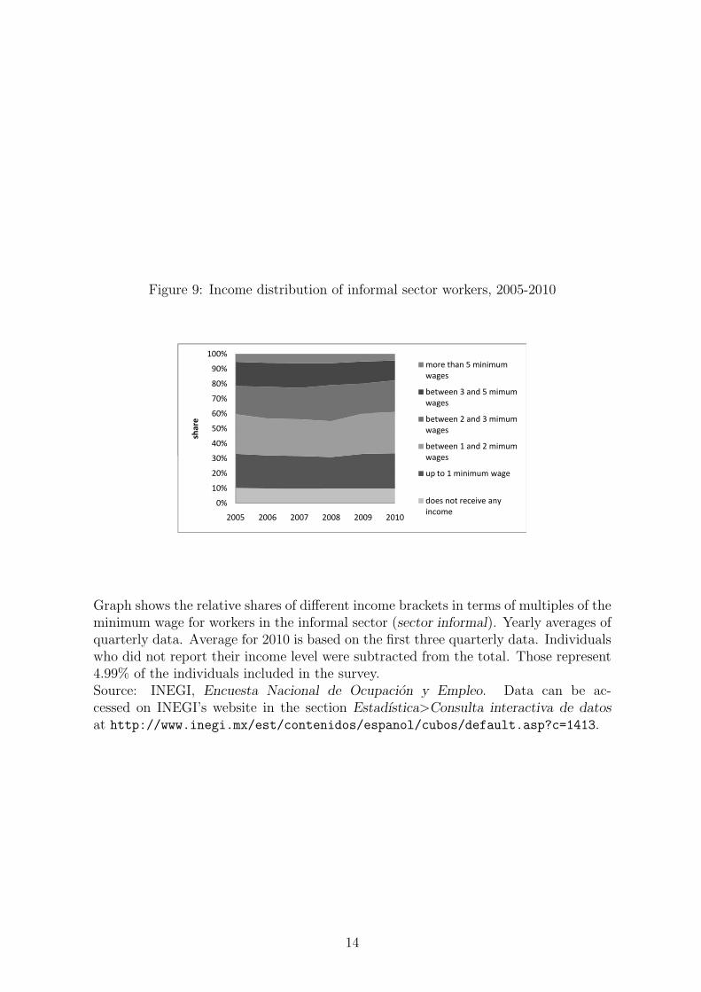
Figure 9: Income distribution of informal sector workers, 2005-2010

30%

40%

50%

60%

70%

80%

90%

100%

share

more than 5 minimum wages

between 3 and 5 mimum wages



0%

10%

20%

30%

40%

50%

60%

70%

80%

90%

100%

2005 2006 2007 2008 2009 2010

share





up to 1 minimum wage

does not receive any income

Graph shows the relative shares of different income brackets in terms of multiples of theminimum wage for workers in the informal sector (sector informal). Yearly averages ofquarterly data. Average for 2010 is based on the first three quarterly data. Individualswho did not report their income level were subtracted from the total. Those represent4.99% of the individuals included in the survey.Source: INEGI, Encuesta Nacional de Ocupacion y Empleo. Data can be ac-cessed on INEGI’s website in the section Estadıstica>Consulta interactiva de datos

at http://www.inegi.mx/est/contenidos/espanol/cubos/default.asp?c=1413.

14

Figure 10: Income distribution of workers in the private sector, 2005-2010

30%

40%

50%

60%

70%

80%

90%

100%

share





0%

10%

20%

30%

40%

50%

60%

70%

80%

90%

100%

2005 2006 2007 2008 2009 2010

share





up to 1 minimum wage

does not receive any income

Graph shows the relative shares of different income brackets in terms of multiples ofthe minimum wage for workers in the private sector (empresas y negocios). Yearlyaverages of quarterly data. Average for 2010 is based on the first three quarterly data.Individuals who did not report their income level were subtracted from the total. Thoserepresent 7.46% of the individuals included in the survey.Source: INEGI, Encuesta Nacional de Ocupacion y Empleo. Data can be ac-cessed on INEGI’s website in the section Estadıstica>Consulta interactiva de datos

at http://www.inegi.mx/est/contenidos/espanol/cubos/default.asp?c=1413.

15

maquila plants are foreign-owned, hence their entry fixed costs are paid from

abroad. After entering, firms draw a productivity ϕ from a Pareto distribution

given by

gj(ϕ) = g(ϕ) = akaϕ−(a+1) (4.5)

which is the same across all sectors. k can be interpreted as the minimum value

of productivity, i.e. ϕ > k, and a > 0 is a shape parameter which governs the

skewness of the distribution. Productivity remains constant and can be used as

a firm identifier. Hence, only firms which get a high enough productivity draw

start production. The entry decision can be described by the per-period profit

of the firm as

πd(ϕH) = pj(ϕ

H)qd(ϕH)− wKK(ϕH)− wLL(ϕ

H)− wI(ϕH)− fjP

Hj (4.6)

where profit of a domestic firm is equal to revenues at home minus factor cost

payments to the two types of labor as well as for the input cost and fixed produc-

tion costs fj . Profits in the manufacturing sector remain in the home economy,

whereas profits frommaquila sales are sent abroad to their foreign owners. Hence,

in the trade balance, entry fixed costs of maquilas enter the domestic economy

and are balanced by the outflow of profits.

Firms face a demand curve with constant elasticity of substitution in the domestic

market:

qHj (ϕ) =αHj Y

H

MH + χFMF(PHj )σ−1pj(ϕ)

−σ (4.7)

where Y H is total income of the home economy and αHj is the expenditure share

on sector j. As we assume that the home economy only consumes the goods

produced in the manufacturing sector, αH1 = 0 and αH2 = 1. Prices at home and

abroad are given by

pHj (ϕ) =wβKjK w

βLjL (τIwI)

1−βKj −βLj

ρϕ(4.8)

ρ = (σ − 1)/σ (4.9)

pFj = τjpHj (4.10)

We follow Demidova and Rodrıguez-Clare (2009) in assuming that domestic firms

do not affect the expenditure level in the foreign economy.8 Still, domestic pro-

8Specifically, we differ from Flam and Helpman (1987) in assuming that domestic firms do not havean impact on the overall price level in the foreign economy.

16

ducers of varieties set prices facing an exogenously given downward sloping de-

mand curve in the foreign economy. Trade costs for final goods τj are symmetric

but can differ across both sectors. τI are the trade costs for the intermediate

good.

The price level in the manufacturing sector in the home economy is given by:

P 1−σ2H =

1

MH2 + χF2 M

F2

[(

MH2 p

H2 (ϕd2H)

)1−σ+ χF2 M

F2

(

τ2ϕd2Fϕx2F

pF2 (ϕx2F )

)1−σ]

Note that this is equal to the overall price level in the domestic economy as

varieties from sector 1 are not consumed. We follow Blanchard and Giavazzi

(2003), Felbermayr et al. (2010) and Larch and Lechthaler (2009) and normal-

ize by (MH)−1/σ where MH is the mass of varieties available in the domestic

economy (i.e. MH =MH1 + χF1 M

F1 ). This ensures that unemployment does not

depend on the size of the economy as the number of varieties does not increase

output as in the standard Dixit-Stiglitz model. As every firm produces a new

variety, ϕ and v can be used interchangeably as firm identifier.

When a firm wants to export, it has to incur additional fixed costs fjx, where

fjx > fj . This fixed cost ranking implies a sorting of firms into exporting. As

maquila plants are set up specifically to reexport their produced varieties, only

firms enter the market which can profitably serve the export market. All fixed

costs, i.e., per period production fixed costs, fHj , per period exporting fixed

costs fHjx, and up-front entry fixed costs fH1e , are in terms of the final good of the

respective industry.

Given this sorting into exporting, one can express the share of firms exporting

by

χHj =1−G(ϕ∗

jx)

1−G(ϕ∗

jd)=

(

ϕ∗

jd

ϕ∗

jx

)a

. (4.11)

where G is the cumulative distribution function of the productivity distribution

g. Note that by construction, χH1 = 1.

We follow Melitz (2003) and define the average productivity of all domestically

active firms:

ϕj =

(

1

1−G(ϕ∗

jd)

∫∞

ϕ∗

jd

ϕσg(ϕ)dϕ

)1/(σ−1)

(4.12)

Similarly, we define the average productivity of all exporting firms as

ϕjx =

(

1

1−G(ϕ∗

jx)

∫∞

ϕ∗

jx

ϕσg(ϕ)dϕ

)1/(σ−1)

(4.13)

17

where ϕ∗

jd and ϕ∗

jx are the cut-off productivities for being active on the domestic

market and on the export market respectively. Profit maximizing firms receive

the following revenues from the domestic and foreign market respectively:

rHj (ϕ) =αjRH

MHj + χFj M

Hj

(PHj )σ−1pHj (ϕ)1−σ (4.14)

rFj (ϕ) =αjRF

MFj + χHj M

Hj

(PFj )σ−1τ1−σj pHj (ϕ)1−σ (4.15)

whereMHj is the mass of domestic firms andMF

j is the mass of foreign firms sell-

ing varieties in the domestic economy. Finally, there is an exogenous probability

of firm death due to force majeure events δ.

4.1 Informality in a search and matching framework

Having introduced the export selection mechanism of our heterogeneous firms

model of international trade in the vein of Melitz (2003) which is the same across

both models of informality, we now turn to describing the features of the labor

market by using search and matching frictions as in Felbermayr et al. (2010).9

We assume that only unskilled labor is “traded” on imperfect labor markets. The

rate of unmatched workers is the share of informal sector employment. Workers

who do not find a job in the formal sector earn b in the informal sector which is a

fraction of the formal sector wage wHL . For a firm, the costs of posting a vacancy

are c and are paid in terms of the final good of industry 2.

The firm posts new vacancies as long as its marginal profit covers the addi-

tional cost of an additional vacancy.

Only a share m of the vacancies v opened by a firm is filled with informal sec-

tor workers. The matching process between informal workers and formal sector

employers is described by a Cobb-Douglas matching function:

m = mθ−γm (4.16)

where θ is the labor market tightness defined as θ = V/U where V is the total

number of vacancies posted and U is the number of informal sector workers. m

measures the overall efficiency of the labor market.

Every match between an informal sector worker and an employer is destroyed

with probability d due to exogenous reasons. Hence, the stock of workers at a

firm evolves according to

Lj,t+1(ϕ) = (1− d)Lj,t(ϕ) +m(θ)vj,t(ϕ) (4.17)

9A similar version of the model was used in Larch and Lechthaler (2009) with sectoral unemploy-ment rates for two skill groups.

18

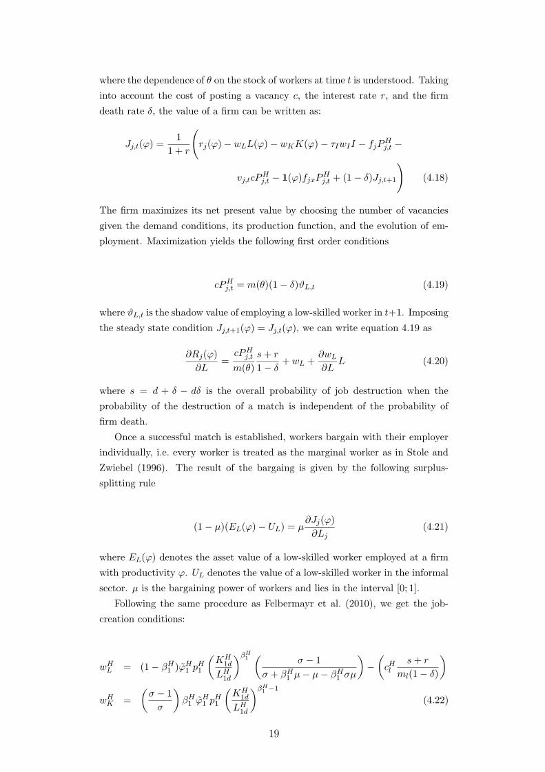
where the dependence of θ on the stock of workers at time t is understood. Taking

into account the cost of posting a vacancy c, the interest rate r, and the firm

death rate δ, the value of a firm can be written as:

Jj,t(ϕ) =1

1 + r

(

rj(ϕ)− wLL(ϕ)− wKK(ϕ)− τIwII − fjPHj,t −

vj,tcPHj,t − 1(ϕ)fjxP

Hj,t + (1− δ)Jj,t+1

)

(4.18)

The firm maximizes its net present value by choosing the number of vacancies

given the demand conditions, its production function, and the evolution of em-

ployment. Maximization yields the following first order conditions

cPHj,t = m(θ)(1− δ)ϑL,t (4.19)

where ϑL,t is the shadow value of employing a low-skilled worker in t+1. Imposing

the steady state condition Jj,t+1(ϕ) = Jj,t(ϕ), we can write equation 4.19 as

∂Rj(ϕ)

∂L=cPHj,tm(θ)

s+ r

1− δ+ wL +

∂wL∂L

L (4.20)

where s = d + δ − dδ is the overall probability of job destruction when the

probability of the destruction of a match is independent of the probability of

firm death.

Once a successful match is established, workers bargain with their employer

individually, i.e. every worker is treated as the marginal worker as in Stole and

Zwiebel (1996). The result of the bargaing is given by the following surplus-

splitting rule

(1− µ)(EL(ϕ)− UL) = µ∂Jj(ϕ)

∂Lj(4.21)

where EL(ϕ) denotes the asset value of a low-skilled worker employed at a firm

with productivity ϕ. UL denotes the value of a low-skilled worker in the informal

sector. µ is the bargaining power of workers and lies in the interval [0; 1].

Following the same procedure as Felbermayr et al. (2010), we get the job-

creation conditions:

wHL = (1− βH1 )ϕH1 pH1

(KH

1d

LH1d

)βH1(

σ − 1

σ + βH1 µ− µ− βH1 σµ

)

−

(

cHls+ r

ml(1− δ)

)

wHK =

(σ − 1

σ

)

βH1 ϕH1 p

H1

(KH

1d

LH1d

)βH1 −1

(4.22)

19

The equilibrium informal sector employment share is then given by

uH =s

s+ θm. (4.23)

Labor market clearing implies:

Le = (1− uH)L (4.24)

L1e = Le − L2e (4.25)

The mass of firms is also pinned down by the labor market equilibirum:

MHj [L(ϕjd) + χHj L(ϕjx)] = (1− uH)L (4.26)

MH1 (KH

1d +KH1xχ

H1 ) +MH

2 (KH2d +KH

2xχH2 ) = KH (4.27)

Total income of the home economy is given by:

Y H = wKK + wLLHe

+ (1− η)PH2 MH1

f1e

r + δ(

kϕH1

)c

1

1− δ+(f1 + χH1 f1x

)(1 + r

1− δ

)

+ PH2 MH2

f2e

r + δ(

kϕH2

)c

1

1− δ+(f2 + χH2 f2x

)(1 + r

1− δ

)

+c

mLHe

(s+ r

1− δ

)

(4.28)

Note that a share of 1−η of the profits in the maquila sector remain in the home

economy, and that we use the manufacturing good as the numeraire.

• θ = 1−δc

[(1−b)(1−µ)

µ wHL −(r+s1−δ

)cm

]

.

Productivity cutoffs, entry and exit:

λH1 = 1 (4.29)

• λH2 = τ2

(PH2PF2

)

(1−α)RH

MH2

+χF2MF

2(1−α)RF

M2(j)+χH2MH

2

fH2xfH2

1σ−1

.

• ϕ∗

1d =(

fH1 + fH1x(λH1)−c) 1c(

1fH1e

) 1c((

1+rr+δ

)(cγ − 1

)

kc) 1c.

• ϕ∗

2d =(

fH2 + fH2x(λH1)−c) 1c(

1fH2e

) 1c((

1+rr+δ

)(cγ − 1

)

kc) 1c.

• ϕ∗

1x = λH1 ϕ∗

1d.

20

• ϕ∗

2x = λH2 ϕ∗

2d.

• ϕ1d =(aγ

) 1σ−1

ϕH1 .

• ϕH2 =(aγ

) 1σ−1

ϕH2 .

• BH1 =

(aγ

) 1σ−1

ϕH1x.

• BH2 =

(aγ

) 1σ−1

ϕH2x.

Prices and expenditure:

•(1−δr+δ

)

pH1 ϕH1

(LH1d)1−β1 (KH

1d

)β1(

1− β1(σ−1σ

)− (1− β1)

(σ−1

σ+β1µ−µ−β1σµ

))

=(ϕH1ϕH1

)σ−1 (1+rr+δ

)

fH1 PH1 .

•(1−δr+δ

)

pH2 ϕH2

(LH2d)1−β2 (KH

2d

)β2(

1− β2(σ−1σ

)− (1− β2)

(σ−1

σ+β2µ−µ−β2σµ

))

=(ϕH2ϕH2

)σ−1 (1+rr+δ

)

fH2 PH2 .

• LH1x = LH1d.

• LH2x =(ϕH2BH2

)1−στ1−σ2

(

(1−α)RF

MF2

+χH2MH

2

)

(

(1−α)RH

MH2

+χF2MF

2

)

(PF2PH2

)σ−1LH2d.

• KH1x =

(ϕH1BH1

)1−στ1−σ1

(

αRF

MF1

+χH1MH

1

)

(

αRH

MH1

+χF1MF

1

)

(PF1PH1

)σ−1KH

1d.

• KH2x =

(ϕH2BH2

)1−στ1−σ2

(

(1−α)RF

MF2

+χH2MH

2

)

(

(1−α)RH

MH2

+χF2MF

2

)

(PF2PH2

)σ−1KH

2d.

• MH1 =

LH1eLH1d+χ

H1 L

H1x.

• MH2 =

LH1eLH1d+χ

H2 L

H1x.

Trade balance:

0 =(PH1)σ−1

τ1−σ1

(ϕF1BF

1

pF1

)1−σ

αRH

MH1 + χF1 M

F1

χF1 MF1

+(PH2)σ−1

τ1−σ2

(ϕF2BF

2

pF2

)1−σ

(1− α)RH

MH2 + χF2 M

F2

χF2 MF2

−(PF1)σ−1

τ1−σ1

(ϕH1BH

1

pH1

)1−σ

αRF

MF1 + χH1 M

H1

χH1 MH1

−(PF2)σ−1

τ1−σ2

(ϕH2BH

2

pH2

)1−σ

(1− α)RF

MF2 + χH2 M

H2

χH2 MH2

+ηΠ1 + τIwI(IH1 + IH2 )

21

4.2 Informality in a fair wages framework

Whereas the search and matching framework more closely resembles the view

of Maloney (2004) on informality where informal sector jobs appear as an exit

option for workers, we will now present a model where informality is a purely

involuntary phenomenon. In this setting, informal sector workers are simply

queuing for formal sector jobs. The theoretical vehicle we use to model this

dualistic view on informality is a fair wages framework as used in Egger and

Kreickemeier (2009). As wages are set above the market-clearing level due to the

fairness considerations of workers, some workers would have to get paid a wage

higher than their marginal productivity. Hence, these workers are not offered a

job in the formal sectors and thus have to work in the informal sector. We assume

that low-skilled workers have a preference for a fair wage wL. This fair wage paid

in the formal sector is a weighted average of the productivity of the firm and the

informal sector employment rate as in Egger and Kreickemeier (2009):

wL(ϕ) = ϕθ[(1− uL)w]1−θ (4.30)

The fair wage hypothesis was introduced by Akerlof and Yellen (1990). Since

then, numerous empirical studies have provided robust evidence that fairness

concerns are a relevant determinant of wages, see Howitt (2002) and Bewley

(2005). When a firm pays the fair wage, workers choose to provide full effort.

If the firm paid only a fraction of the fair wage, workers would provide only

a fraction of their maximum effort. This implies that the firm is indifferent

between paying the fair wage or less, as output in efficiency units remains the

same.10 Therefore, we assume that the firm pays the fair wage when it does not

reduce its profits.

to be completed...

The ratio of cut-off revenues, i.e. of zero (export) profits is given by

rHirFi

=σfiP

Hi

σfixPFi⇒

RHMHi +χFi M

Hi

(PHi )σ−1PHi (ϕ∗

i )1−σ

RFMFi +χHi M

Hi

(PFi )σ−1τ1−σi PHi (ϕ∗

ix)1−σ

=fifix

(4.31)

Now plug in price of variety (4.8):

τσ−1i

RHMHi +χFi M

Hi

RFMFi +χHi M

Hi

(PHiPFi

)σ−1

wβKiK wL(ϕ

∗

i )βLi w

1−βKi −βLiI /(ρϕ∗

i )

wβKiK wL(ϕ∗

ix)βLi w

1−βKi −βLiI /(ρϕ∗

ix)

1−σ

=fifix

Then cancel stuff and plug in the fair wage constraint (4.30):

10For details, see Akerlof and Yellen (1990).

22

τσ−1i

RHMHi +χFi M

Hi

RFMFi +χHi M

Hi

(PHiPFi

)σ−1[(

ϕ∗

i

ϕix

)θβLi −1]1−σ

=fifix

(4.32)

Define ξi = (1− σ)(θβLi − 1) and solve for the cut-off ratio:

ϕ∗

ix

ϕi=

RHMHi +χFi M

Fi

RFMFi +χHi M

Hi

(PHiPFi

)σ−1

τσ−1i

fixfi

1/ξi

︸︷︷︸

(4.33)

⇒ ϕ∗

ix = Λ1/ξii ϕ∗

i (4.34)

average productivity of all firms which are active domestically ⇒ Mario’s A

ϕi =

(

1

1−G(ϕ∗

i )

∫∞

ϕ∗

i

ϕξi g(ϕi)dϕi

)1/ξi

(4.35)

(4.36)

Assume that ξi < a, then the integral converges and we have

ϕid =

(a

a− ξi

)1/ξi

ϕ∗

i (4.37)

average productivity of all exporting firms ⇒ Mario’s B

ϕix =

(

1

1−G(ϕ∗

i )

∫∞

ϕ∗

ix

ϕξi g(ϕi)dϕi

)1/ξi

(4.38)

= (ϕ∗

i )a/ξi a1/ξi

{[1

ξi − aϕξi−ai

]∞

ϕ∗

ix

}1/ξi

(4.39)

(4.40)

Remember the cut-off relation given by (4.34) and again assume that ξi < a,

then the integral converges and we have

ϕix =

(a

a− ξi

)1/ξi

Λξi−a

ξ

i ϕ∗

i (4.41)

Deriving the labor demand for a firm with productivity ϕi yields

∂π

∂K=

σ − 1

σ(RH)1/σ(PHi )(σ−1)/σβKi ϕidK

βKi −1i L

βLii I

1−βLi −βKi

i = wK

∂π

∂L=

σ − 1

σ(RH)1/σ(PHi )(σ−1)/σβLi ϕ

1−θid K

βKii L

βLi −1i I

1−βLi −βKi

i = [(1− uL)wL]1−θ

∂π

∂I=

σ − 1

σ(RH)1/σ(PHi )(σ−1)/σβIi ϕidK

βKii L

βLii I

−βLi −βKi

i = wI

23

Free entry condition: NPV of average profit per firm equals entry costs

[1−G(ϕ∗

i )]πiδ

= PHi fei (4.42)

[1−G(ϕ∗

i )]

∫∞

ϕ∗

i

πd(ϕi)g(ϕi)dϕi + χi

∫∞

ϕ∗

ix

πx(ϕi)g(ϕi)dϕi = δPHi fei (4.43)

5 Policy experiments

Having set up the two models, we solve them numerically to get comparative

static results. In order to obtain analytical results, we would have to simplify

our model considerably which would preclude any comparison with the actual

Mexican experience. Numerical solutions have gained importance for the analysis

of international trade models in recent years, see e.g. Anderson and van Wincoop

(2003), Bernard, Eaton, Jensen, and Kortum (2004), Bernard et al. (2007), and

Helpman and Itskhoki (2010).

5.1 Calibration of search and matching model

5.1.1 Parameter values

We assume that the maquila sector is low-skilled labor intensive (βL1 = 0.3,

βK1 = 0.1), whereas the standard manufacturing sector is high-skilled intensive

(βK2 = 0.6). We closely follow Felbermayr et al. (2010) and set the parameters

of the Pareto distribution as in their paper (k = 0.2, a = 3.4). The probability

of firm death is set to δ = 0.11. The interest rate is set to r = 0.04. Following

Bernard et al. (2007), we set the elasticity of substitution σ = 3.8. In our baseline

scenario, all profits may be shifted abroad (η = 1). The entry fixed costs are set

equal to fie = 0.1 in both sectors. Per period production fixed costs are equal

to fi = 2 in both sectors. The ratio of entry fixed costs to exporting fixed costs

is 1.93. This implies that approximately 22% of all manufacturing firms export,

which is in line with Bernard et al. (2004). Trade costs of the final maquila

good are set to τ1 = 1.5, for the final manufacturing good τ2 = 1.2, and for the

intermediate good τI = 1.5. The price for the intermediate good is set to wI = 1,

the relative price of the maquila good vs. the manufacturing good is set equal

to 5. We set the informal sector income to 50% of the formal sector wage of

unskilled workers. The elasticity of the matching function is set to γ = 0.5 as

in Petrongolo and Pissarides (2001). The productivity of the matching function

is set to m = 7.6, the exogenous rate of job destruction is set to d = 0.3. The

bargaining power of the worker is set to µ = 0.5.

24

Figure 11: Comparative statics of the final good price in the maquila sector

Further details can be found in the appendix.

We analyze the effect of different policy changes:

1. rise in the relative price of the maquila good

2. fall in the profit tax in the maquila sector

3. reduction in the fixed exporting costs in the maquila sector

4. reduction of maquila/intermediate trade costs

5.1.2 A rise in the final maquila good price

Result 1. A rise in the final maquila good price will decrease the informal sector

and increase welfare in the home economy. Welfare will be unambiguously higher

in an economy with an informal sector than in an economy where the informal

sector is shut down.

As can be seen in figure 11, an exogenous rise in the price of the final maquila

good will decrease the informal sector and increase domestic welfare, a result in

line with standard trade models. We resimulate the model without any labor

market rigidities, i.e. we shut down the informal sector. All other parameter

settings remain equal. For all prices of the final maquila good, welfare will be

higher in the economy with an informal sector. Also the gradient of the increase

in welfare is higher in the economy with the informal sector. A higher price of the

maquila good increases relative demand for low-skilled workers as the maquila

sector is low-skilled intensive. This props up wages for low-skilled workers. What

is more, low-skilled workers have to be offered a higher wage. If the wage paid

in the formal sector is too low, workers will opt out of the bargaining and start

a business in the informal sector. This threat of the exit option forces employers

to pay more to their employees. This reduces profits. As the increase in the

maquila sector will also increase profits transferred abroad, the threat of the exit

25

option will leave more income in the domestic economy and directly increase

welfare. When the informal sector is shut down, workers cannot use informal

sector employment. In a perfectly competitive labor market, workers have no

bargaining power and are simply paid as their marginal productivity implies.

This implies higher profits for the foreign owned companies. Hence, workers do

not profit as much from the increase in the final maquila good price as in the

model economy with an informal sector.

5.1.3 A reduction in the profit tax in the maquila sector

to be added

5.1.4 A fall in exporting fixed costs in the maquila sector

Result 2. A fall in the exporting fixed costs in the maquila sector will increase

the informal sector and decrease welfare in the home economy. Welfare will be

unambiguously higher in an economy with an informal sector than in an economy

where the informal sector is shut down.

The domestic government may create programs which specifically reduce the

exporting fixed costs in the maquila sector to attract multinational enterprises.

Programs may include simplified customs procedures, a general cut in red tape

or efforts to reduce corruption or increase general efficiency of government agen-

cies. As can be seen in figure 12, a reduction in exporting fixed costs in the

maquila sector decreases welfare. Shutting down the possibility of employment

in the informal sector, we again resimulate the model. Comparing both model

economies with the same parameter values, again welfare is higher across all con-

sidered values of exporting fixed costs in the economy with the informal sector.

A reduction in exporting fixed costs in the maquila sector increases the size of

the maquila sector and increases profits for multinational enterprises operating

there. As profits are going abroad, less income remains in the home economy,

overall consumption is lower and hence domestic welfare. Again the possibility of

employment in the informal sector is a credible threat of low-skilled workers and

therefore preps up their wage. This keeps more profits in the domestic economy

and directly leaves more income for domestic consumption directly increasing

domestic welfare.

5.1.5 A differential fall in trade costs in the maquila sector

Result 3. A differential fall in trade costs for the final maquila good will decrease

the informal sector and decrease welfare in the home economy. Welfare will be

unambiguously higher in an economy with an informal sector than in an economy

where the informal sector is shut down.

26

Figure 12: Comparative statics of exporting fixed costs in the maquila sector

As can be seen in the left panel of figure 13, a differential fall in trade costs for

shipping the final maquila good abroad decreases welfare in the home economy.

A fall in iceberg trade costs implies that less output has to be produced to ship

one unit to consumers in the foreign economy. At the same time, demand for the

maquila good increases as its goods are cheaper for foreign consumers and the

maquila sector expands. However, Mexican consumers do not profit from the fall

in trade costs as they do not consume the good. What is more, the increase of

the maquila sector comes at the expense of the standard manufacturing sector.

The latter sector is domestically owned, whereas the maquila sector is foreign-

owned. Hence, the expansion of the maquila sector increases the overall amount

of profits sent out of the home economy directly decreasing available income

for domestic consumption and hence decreasing overall welfare. Thus the home

country over-specializes in the production of the maquila good. Note also that

the fall in trade costs is accompanied by a decrease in the informal sector. Hence,

two obvious measures of political success as an increase of multinationals in the

maquila sector as well as the reduced informal sector would indicate an improve-

ment of domestic welfare. Resimulating the model without the informal sector,

we again find that welfare is lower across all considered trade cost values in the

economy without the possibility of informal sector employment. The mechanism

at work is again the exit option of low-skilled workers which retains more income

for consumption in the home economy. The counter factual fall in informal sec-

tor employment in our model simulations compared to the actual experience of

Mexico can be rationalized by recognizing countervailing effects of trade liber-

alization on informality as indicated by Marjit et al. (2007). Their channel of

higher corruption due to trade liberalization increases informal employment is

not present in our model. Empirically, it may well be that both effects exactly

set off each other leading to the observed pattern of informality. Furthermore,

the fall in the informal sector size is very small, contradicting the expected bigger

27

Figure 13: Comparative statics of trade costs for the final maquila good

effect of the expansion of maquilas on informal sector employment.

Result 4. Comparing two model economies with and without an informal sec-

tor, welfare will be higher in the economy with the informal sector across all

comparative static exercises.

5.2 Calibration of fair wages model

to be added...

6 Robustness checks

In order to check the robustness of our results, we also simulate our models by

allowing consumption of the maquila good also in the home economy. Hence,

preferences are given by

UH = (CH1 )α1(CH2 )α2 (6.1)

with α1 + α2 = 1.

DATA ON MEXICAN CONSUMPTION OF MAQUILA GOODS?

to be added...

To see whether our results crucially hinge on the specific form of small country

assumption we use, we simulate a two country version of our model where the

small economy is characterized by an informal labor market whereas in the large

economy, labor markets are perfectly competitive. RESULTS TO BE ADDED

28

7 Estimation

We will try to fit key moments of the data with our model in order to get estimates

of the different fixed costs of production. We will then use the estimated model

to counter factually shut down the informal sector and study the implied welfare

changes.

We minimize the following objective function

θ = argminθ

(g(θ)− g(∆))′ I (g(θ)− g(∆)) (7.1)

where θ = (fx1, f2, fe2/fe1, fx2)′ is the parameter vector, ∆ is the data, I is the

identity matrix, and g(θ) is a (M × 1) vector of moment conditions. Note that

f1 = 0.

g(θ) =

g1

g2

g3

g4

=

relative size of manufacturing to maquila

average size of maquila

average size of manufacturing

share of exporters manufacturing

(7.2)

=

R1/R2 −R1/R2

rx1 (φ)− rx1 (φ)

(rd2(φ) + rx2 (φ))− (·)

χ2 − χ2

⇒ fe2/fe1

⇒ fx1

⇒ f2

⇒ fx2

(7.3)

Results to be included.

8 Conclusion

This paper has investigated the relationship between the rise of the maquila sec-

tor in Mexico, its linkages to informal sector employment as well as its broader

implications for Mexican welfare. Our simulations of a small open economy with

heterogeneous firms and labor market rigidities for low-skilled workers indicate

that a reduction in plant set up costs in the maquila sector like a reduction

of red tape and other non-tariff barriers to trade and foreign direct investment

lead to a decrease in general welfare. Most of the newly created jobs in the in-

termediate input processing plants sector replace standard manufacturing jobs

without inducing a major decrease in informal sector employment. The decline

in informality is accompanied by a general decline of welfare. Even though stan-

dard measures of political achievement like an increase in overall formal sector

employment as well as an increase of foreign-owned plants seem to indicate a

positive development of the model economy, welfare actually declines. This is

due to XXX, WHAT HAPPENS TO RELATIVE WAGES (W/, W/O informal

29

sector?). Hence, there arises a distributional conflict between high-skilled work-

ers who prefer a stricter stance on informality whereas low-skilled workers prefer

a two-tier labor market. Our results suggest that the presence of a large infor-

mal sector is not necessarily detrimental to general welfare in an economy, at

least given the level of development and its general production and consumption

structure. What is more, the reduction of informality creates a new distributional

conflict between high-skilled and low-skilled workers which has been overlooked

both in the theoretical literature as well as in policy discussions so far. The

results also indicate that labor market rigidities may create intricate choices for

policy makers as increasing formal sector employment and restricting access to

informal jobs in order to increase tax revenues and payments to pension sys-

tems may well be detrimental to voters’ welfare. This highlights the importance

of future research on informality to uncover its Janus-faced nature in order to

enlighten policy choices faced by emerging economies.

References

Akerlof, G. A. and J. L. Yellen (1990): “The fair wage-effort hypothesis

and unemployment,”Quarterly Journal of Economics, 105, 255–283.

Anderson, J. E. and E. van Wincoop (2003): “Gravity with gravitas: A

solution to the border puzzle,”American Economic Review, 93, 170–192.

Attanasioa, O., P. K. Goldberg, and N. Pavcnik (2004): “Trade reforms

and wage inequality in Colombia,” Journal of Development Economics, 74,

331–366.

Bernard, A. B., J. Eaton, J. B. Jensen, and S. Kortum (2004): “Plants

and productivity in international trade,” American Economic Review, 93,

1268–1290.

Bernard, A. B. and J. B. Jensen (1999): “Exceptional exporter performance:

cause, effect, or both?” Journal of International Economics, 47, 1–25.

——— (2004): “Why some firms export,” Review of Economics and Statistics,

86, 561–569.

Bernard, A. B., S. J. Redding, and P. K. Schott (2007): “Comparative

advantage and heterogeneous firms,”Review of Economic Studies, 74, 31–66.

Bewley, T. (2005): “Fairness, reciprocity, and wage rigidity,” in Moral Senti-

ments and Material Interests: The Foundations of Cooperation in Economic

Life, ed. by H. Gintis, S. Bowles, R. Boyd, and E. Fehr, Cambridge: MIT

Press, 303–338.

30

Bhagwati, J. (1958): “Immiserizing growth: A geometrical note,” Review of

Economic Studies, 25, 201–205.

Blanchard, O. and F. Giavazzi (2003): “Macroeconomic effects of regu-

lation and deregulation in goods and labor markets,” Quarterly Journal of

Economics, 118, 879–907.

Chandra, V. and M. A. Khan (1993): “Foreign investment in the presence of

an informal sector,” Economica, 60, 79–103.

Demidova, S. and A. Rodrıguez-Clare (2009): “Trade policy under firm-

level heterogeneity in a small economy,” Journal of International Economics,

78, 100–112.

Egger, H. and U. Kreickemeier (2009): “Firm heterogeneity and the la-

bor market effects of trade liberalization,” International Economic Review, 50,

187–216.

Felbermayr, G., J. Prat, and H.-J. Schmerer (2010): “Globalization and

labor market outcomes: Wage bargaining, search frictions, and firm hetero-

geneity,” Journal of Economic Theory, forthcoming.

Flam, H. and E. Helpman (1987): “Industrial policy under monopolistic com-

petition,” Journal of International Economics, 22, 79–102.

Gasparini, L. and L. Tornarolli (2009): “Labor informality in Latin Amer-

ica and the Caribbean: Patterns and trends from household survey microdata,”

Desarollo y Sociedad, 13–80.

Graham, E. M. and E. Wada (2000): “Domestic reform, trade and invest-

ment liberalisation, financial crisis, and foreign direct investment into Mexico,”

World Economy, 23, 777–797.

Harris, J. R. and M. P. Todaro (1970): “Migration, unemployment and

development: A two-sector analysis,” American Economic Review, 60, 126–

142.

Helpman, E. and O. Itskhoki (2010): “Labour market rigidities, trade and

unemployment,”Review of Economic Studies, 77, 1100–1137.

Howitt, P. (2002): “Looking inside the labor market: A review article,”Journal

of Economic Literature, 40, 125–138.

ILO (1993): Resolution concerning statistics of employment in the informal sec-

tor, adopted by the Fifteenth International Conference of Labour Statisticians,

Geneva: International Labor Organization (ILO).

31

INEGI (2010): Mexico at a glance 2010, Instituto Nacional de Estadıstica y

Geografıa (INEGI).

Jutting, J. P. and J. R. de Laiglesia, eds. (2009): Is informal normal?

Towards more and better jobs in developing countries, Paris: OECD.

Keuschnigg, C. and E. Ribi (2009): “Outsourcing, unemployment and welfare

policy,” Journal of International Economics, 78, 168–176.

Larch, M. and W. Lechthaler (2009): “Comparative advantage and skill-

specific unemployment,” CESifo Working Paper No. 2754.

Maloney, W. F. (2004): “Informality revisited,”World Development, 32, 1159–

1178.

Marjit, S., S. Ghosh, and A. Biswas (2007): “Informality, corruption and

trade reform,” European Journal of Political Economy, 23, 777–789.

Martin, G. (2000): “Employment and unemployment in Mexico in the 1990s,”

Monthly Labor Review, 123, 3–18.

Melitz, M. (2003): “The impact of trade on intra-industry reallocations and

aggregate industry productivity,” Econometrica, 71, 1695–1725.

Mollick, A. V. (2008): “The rise of the skill premium in Mexican maquilado-

ras,” Journal of Development Studies, 44, 1382–1404.

Paus, E. A. and K. P. Gallagher (2008): “Missing links: Foreign investment

and industrial development in Costa Rica and Mexico,”Studies in Comparative

International Development, 43, 53–80.

Pavcnik, N. (2002): “Trade liberalization, exit, and productivity improvements:

Evidence from Chilean plants,”Review of Economic Studies, 69, 245–276.

Petrongolo, B. and C. A. Pissarides (2001): “Looking into the black box:

A survey of the matching function,” Journal of Economic Literature, 39, 390–

431.

Ramirez, M. D. (2006): “Is foreign direct investment beneficial for Mexico? An

empirical analysis, 1960-2001,”World Development, 34, 802–817.

Satchi, M. and J. Temple (2009): “Labor markets and productivity in devel-

oping countries,”Review of Economic Dynamics, 12.

Stole, L. A. and J. Zwiebel (1996): “Intra-firm bargaining under non-binding

contracts,”Review of Economic Studies, 63, 375–410.

32

Ulyssea, G. (2010): “Regulation of entry, labor market institutions and the

informal sector,” Journal of Development Economics, 91, 87–99.

Waldkirch, A., P. Nunnenkamp, and J. E. A. Bremont (2009): “Employ-

ment effects of FDI in Mexico’s non-maquiladora manufacturing,” Journal of

Development Studies, 45, 1165–1183.

33

A Parameter settings for model simulations

for search and matching model

The calibration closely follows Bernard et al. (2007) and on the labor market

side Felbermayr et al. (2010).

Parameters for exogenous large foreign country F :

• MF1 = 10.

• MF2 = 10.

• XF1 = 0.3.

• XF2 = 0.3.

• AF1 = 0.5.

• AF2 = 0.5.

• BF1 = 0.8.

• BF2 = 0.8.

• pF1 = 1.

• pF2 = 1.

General parameters:

• N = 1, denoted in the subsequent with superscript H (for home country).

• fH1 = 0.1.

• fH2 = 0.1.

• fH1e = 2.

• fH2e = 2.

• fH1x = f1 × 1.93.

• fH2x = f2 × 1.93.

• δ = 0.11.

• τ1 = [1...0.05...1.6].

• τ2 = [1...0.05...1.6].

• α = 0.5.

• σ = 3.8.

• ς = 1− 1/σ.

Technological assumptions:

• Good 1 capital-intensive: β1 = 0.6.

• Good 2 labor-intensive: β2 = 0.4.

34

Assumption about the Pareto distribution:

• k = 0.2.

• c = 3.4.

• γ = c− σ + 1.

• ξ = c(kc−γ)/γ.

Job Market parameter assumptions:

• cl = 0.134.

• r = 0.04.

• ρ = 0.3.

• s = ρ+ δ − ρδ.

• µ = 0.5.

• m = 7.6.

• γm = 0.5.

• b = 0.4.

Factor endowments are assumed as follows:

• LH = 1000.

• KH = 1200.

B Model with one-shot matching

For this model, we use a simplified version of a search and matching model as

presented in Keuschnigg and Ribi (2009). In this modelling context, the whole

labor supply is assumed to be working in the informal sector and all workers

start to search for a potential employer either in the domestic manufacturing

sector or in the maquila industry. Once a successful match has been established,

workers remain at their employer forever, hence the term one-shot matching.

This simplification gets rid of the dynamics and hence of much of the analytical

complexities without sacrificing the richer model structure of the search and

matching framework.

B.1 Assumptions

• We have two industries: maquiladora (1) and regular manufacturing (2)

• All the output from the maquiladora sector is exported

• There is a measure 1 of unskilled workers and a measure H of skilled work-

ers. Labor market for unskilled workers is imperfectly competitive

35

B.2 Preferences

• Consumers at Home only care about good 2, hence,

U = C2, (B.1)

C2 =

( n2∑

i=1

dσ−1σ

2i +

n∗

2∑

i=1

(d∗2i)σ−1σ

) σσ−1

. (B.2)

• There is a large country with which Home trades, so we take as given n∗1,

n∗2 and the prices of these varieties, which we set equal to 1 + t1 and 1 + t2

in sector 1 and 2 respectively.

• Preferences in the large foreign country are given by:

U∗ = (C∗

1 )1−α(C∗

2 )α. (B.3)

B.3 Maquiladora Sector

• Production in sector 1 is given by:

q1i = A1lβi1h

1−βi1 . (B.4)

• The matching function for unskilled workers is given by:

M(u, v) =uv

[uψ + vψ

] 1ψ

, ψ ∈ (0, 1) ⇒ (B.5)

M(1, v) =v

[1 + vψ

] 1ψ

. (B.6)

the reason behind this particular functional form for the matching function

is that it insures that q(θ), e(θ) ∈ [0, 1].

• since u = 1, we have that market tightness is given by θ ≡ v/u = v. Define

q(θ) as the probability of filling a vacancy and e(θ) the probability of finding

a job. Then:

q(θ) =M(1, v)

v=

1[1 + vψ

] 1ψ

, (B.7)

e(θ) =M(1, v)

1=

v[1 + vψ

] 1ψ

= vq(θ), (B.8)

e(θ) = θq(θ). (B.9)

In equilibrium, L1 = n1l1i = e(θ), which results in:

v = L1

(1

1− Lψ1

) 1ψ

. (B.10)

36

• The cost of posting a vacancy is k (denominated in units of skilled labor).

So, if a firm wants to employ l1i workers, it needs to post q(θ)v vacancies,

that is l1i = vq(θ). Therefore, given the unskilled wage, wl, the cost of

employing one worker is

Wl = wl +k

q(θ). (B.11)

• The unit cost of production in sector 1 is:

mc1 = A−11 [β−β(1− β)−(1−β)]W β

l w1−βh . (B.12)

• Demand for sector 1’s output comes only from abroad:

q1i = d∗1i =p−σ1i (1− α)E∗

∑n1j=1 p

1−σ1j + n∗1(1 + t1)1−σ

. (B.13)

with

P1 =

[ n1∑

j=1

p1−σ1j + n∗1(1 + t1)1−σ

] 11−σ

=

[

n1p1−σ1 + n∗1(1 + t1)

1−σ

] 11−σ

. (B.14)

since p1i = p1 = (σ/(σ − 1))mc1

• To find out the optimal factor demands for firms in sector 1, we solve the

following problem (dropping out the i indices since, the solution is identical

for all firms):

π = maxl1,h1

{

[(1− α)E∗]P σ−11 (lβ1h

1−β1 )1−1/σ − whh1 −Wll1

}

. (B.15)

which results in the following F.O.Cs:

(σ − 1

σ

)

[(1− α)E∗]1σP

σ−1σ

1 (A1lβ1h

1−β1 )−1/σ(1− β)A1l

β1h

−β1 = wh,

(MRPh = wh)(σ − 1

σ

)

[(1− α)E∗]1σP

σ−1σ

1 (A1lβ1h

1−β1 )−1/σβA1l

β−11 h1−β1 =Wl

(MRPl =Wl)

hence, we have that MRPl = wl +kq(θ) .

• The unskilled labor wage is determined by Nash bargaining solution. We

assume that the outside option of unemployed workers is zero. Then

wl = maxwl

{

wγl (MRPl − wl)1−γ

}

. (B.16)

37

which results in

wl =γ

1− γ(MRPl − wl), (B.17)

=γ

1− γ

k

q(θ). (B.18)

• The number of firms in sector 1 is pinned down by the zero profit condition:

(1− α)E∗P σ−11 p1−σ1 = σf1. (B.19)

• Since all the output of sector 1 is exported, net exports are given by:

Net Exports1 = n1p1q1 = n1(1− α)E∗P σ−11 p1−σ1 . (B.20)

• Skilled labor used in sector 1:

H1 = n1h1 + n1f1 + kv. (B.21)

B.4 Manufacturing Sector

• Production: q2i = A2h2i, which implies that the marginal cost of production

is mc2 = wh/A2

• Demand:

d2i =p−σ2i E

∑n2j=1 p

1−σ2j + n∗2(1 + t2)1−σ

, (B.22)

d∗2i =p−σ2i αE

∗

∑n2j=1 p

1−σ2j + n∗2(1 + t2)1−σ

(B.23)

q2i = d2i + d∗2i =p−σ2i (E + αE∗)

∑n2j=1 p

1−σ2j + n∗2(1 + t2)1−σ

. (B.24)

• Demand for imported varieties in sector 2 is given by:

df2i =(1 + t2)

−σE∑n2

j=1 p1−σ2j + n∗2(1 + t2)1−σ

. (B.25)

• If wh is the numeraire, then, optimal pricing is:

p2i = p2 =σ

σ − 1

1

A2. (B.26)

and the price index P2 is given by:

P2 =

[

n2p1−σ2 + n∗2(1 + t2)

1−σ

] 11−σ

. (B.27)

38

which results in quantity per firm:

q2i = q2 = (E + αE∗)P σ−12 p−σ2 . (B.28)

• Demand for skilled labor (we assume that the fixed cost of production is

denominated in units of skilled labor):

H2 = n2

(q2A2

+ f2

)

. (B.29)

• The number of firms in sector 2 is pinned down by the zero profit condition:

(E + αE∗)P σ−12 p1−σ2 = σf2. (B.30)

• Total domestic income is given by:

E = wlL1 +H. (B.31)

• Net exports in sector 2 are given by:

Net Exports2 =1

n2p1−σ2 + n∗2(1 + t2)1−σ

[n2αE

∗p1−σ2i − n∗2E(1 + t2)1−σ].

(B.32)

B.5 Market Clearing

An equilibrium is given by a vector of variables (n1, n2, E∗, l1, h1) such that:

1. Zero profit conditions for both sectors are satisfied, equations (B.19) and

(B.30)

2. The first order conditions for l1 and h1 are satisfied, equations (MRPh =

wh) and (MRPl =Wl)

3. Market clearing in the skilled labor market: H1+H2 = H, equations (B.21)

plus (B.29)

If the model is correctly written, then the balanced trade condition should

also be satisfied:

Net Exports1 +Net Exports2 = 0. (B.33)

So we have:

(1− α)E∗P σ−11 p1−σ1 = σf1. (B.34)

(E + αE∗)P σ−12 p1−σ2 = σf2. (B.35)

39

(σ − 1

σ

)

[(1− α)E∗]1σP

σ−1σ

1 (A1lβ1h

1−β1 )−1/σ(1− β)A1l

β1h

−β1 = wh, (B.36)

(σ − 1

σ

)

[(1− α)E∗]1σP

σ−1σ

1 (A1lβ1h

1−β1 )−1/σβA1l

β−11 h1−β1 =Wl. (B.37)

n1h1 + n1f1 + kv︸︷︷︸

H1

+n2

(q2A2

+ f2

)

︸︷︷︸

H2

= H. (B.38)

B.6 Comparative Statics

B.6.1 Benchmark

We study the comparative statics resulting from an increase in 1 + t1, the world

price of the maquiladora good.

Figure 14: Comparative Statics - Increase in 1 + t1

0 50.06

0.08

0.1

0.12

wl

1+t1

0 50.25

0.3

0.35

0.4

0.45

Wl

1+t1

0 50.5

1

1.5

P1

1+t1

0 5

0.3

0.32

0.34

P2

1+t1

0 50.05

0.1

0.15

0.2

0.25

NX1

1+t1

0 5−0.2

−0.15

−0.1

−0.05

0

NX2

1+t1

0 50.05

0.1

0.15

0.2

0.25

L1

1+t1

0 50.8

0.85

0.9

0.95

1Informal

1+t1

0 50.2

0.4

0.6

0.8

1

n1

1+t1

0 54.2

4.4

4.6

4.8

5

n2

1+t1

0 53.1

3.2

3.3

3.4

3.5Welfare

1+t1

0 50.4

0.5

0.6

0.7

0.8E*

1+t1

Intuition: when (1 + t1) increases, this has a positive direct effect on P1. In

order to maintain the zero profit condition in sector 1, we need n1 to increase

(higher foreign prices will induce entry in the domestic market). To be com-

pleted...

Informal = 1− L1 (B.39)

40

Welfare =E

P2(B.40)

Table 1: Comparative Statics - Other Variables

Variable Direction of Change

qi1 ↓

Q1 = n1qi1 ↑

li1 ↓

L1 = n1li1 ↑

hi1 no changeqi2 no changeQ2 = n2qi2 ↓

hi2 no changev ↑

B.6.2 Home Country Consumes Good 1

In this case we allow for the Home country to consume good 1. We assume

α = 0.1 and αf = 0.5 (in this scenario, αf denotes the weight of good 1 in

foreign consumers’ utility).

B.6.3 Sector 2 Also Uses Unskilled Labor

Under this scenario, equation (B.10) becomes:

v =L1 + L2

(1− (L1 + L2)ψ

) 1ψ

(B.41)

the marginal cost of production for good 2 becomes (assuming β1 > β2):

mc2 = A−12 [β−β22 (1− β2)

−(1−β2)]W β2l w1−β2

h . (B.42)

41

Figure 15: Comparative Statics - Home Country Consumes Good 1

0 50.2

0.22

0.24

0.26

wl

1+t1

0 50.85

0.9

0.95

1

1.05

Wl

1+t1

0 50.4

0.5

0.6

0.7

P1

1+t1

0 5

0.8

1

1.2

1.4

P2

1+t1

0 5−0.2

−0.1

0

0.1

0.2

NX1

1+t1

0 5−0.2

−0.1

0

0.1

0.2

NX2

1+t1

0 50.36

0.38

0.4

0.42

L1

1+t1

0 5

0.58

0.6

0.62

0.64Informal

1+t1

0 54

4.5

5

5.5

6

n1

1+t1

0 5−0.5

0

0.5

1

1.5

n2

1+t1

0 51.8

2

2.2

2.4

2.6Welfare

1+t1

0 50

0.5

1

1.5E*

1+t1

42

Figure 16: Comparative Statics - Sector 2 Also Uses Unskilled Labor

0 50.24

0.25

0.26

0.27

0.28

wl

1+t1

0 50.95

1

1.05

1.1

1.15

Wl

1+t1

0 50.4

0.45

0.5

0.55

0.6

P1

1+t1

0 50.8

1

1.2

1.4

1.6

P2

1+t1

0 50

0.1

0.2

0.3

0.4

NX1

1+t1

0 5−0.4

−0.3

−0.2

−0.1

0

NX2

1+t1

0 50.35

0.4

0.45

0.5

L1

1+t1

0 5

0.58

0.6

0.62Informal

1+t1

0 54.5

5

5.5

6

6.5

n1

1+t1

0 5−1

−0.5

0

0.5

1

n2

1+t1

0 51.8

2

2.2

2.4

2.6Welfare

1+t1

0 50.8

1

1.2

1.4

1.6E*

1+t1

43

The rise of the maquiladoras: Labor market consequences of offshoring in developing countries

Documents

Transcript of The rise of the maquiladoras: Labor market consequences of offshoring in developing countries