THE RESEARCH PROPOSAL TEMPLATE - CORE

Tools for Evaluating Fault Detection and

Diagnostic Methods for HVAC Secondary

Systems

A Thesis

Submitted to the Faculty

Of

Drexel University

By

Shokouh Pourarian

in partial fulfillment of the

requirements for the degree

of

Doctor of Philosophy

December, 2015

Dissertation approval form

ii

ACKNOWLEDGMENTS

Ostensibly, this dissertation represents the consummation of my PhD work. In

reality, it represents thirty years of patient and thoughtful support from family, friends

and all my teachers and mentors. In this regard I would like to acknowledge all who

contributed to this journey for such a long time. In particular, I must express my

appreciation to Dr. Jin Wen who granted me the opportunity to pursue the doctoral

degree at Drexel University. In the last five years, she has emerged as a trusted guide

and invaluable mentor for this work.

To Dr. Daniel A. Veronica, Dr. Anthony José Kearsley and Dr. Amanda

Pertzborn from National Institute of Standard and Technology: I extend special

appreciation for their dependable, serious, and accurate guidance, input and support

during the accomplishment of this work.

To members of my committee, Dr. Amanda Pertzborn (National Institute of

Standard and Technology), Dr. Xiaohui Zhou (Iowa Energy Center), Dr. Patrick L.

Gurian and Dr. Michael Waring (Drexel- Civil, Architectural and Environmental

Engineering): thank you for reviewing my dissertation and your valuable inputs.

The developed testbeds in this thesis were validated using experimental data

provided by Iowa Energy Center. I would like to thank Dr. Xiaohui Zhou and Dr. Ran

Liu from this center for their support, help as well as patience in answering the

questions.

I would like to express my gratitude to the U.S. National Institute of Standard and

Technology for financially sponsoring my researches and providing this wonderful

opportunity to pursue my PhD.

I appreciate all my BSEG lab mates specially Xiwang Li for his generous

collaboration and Jared Langevin for his perpetual company and encouragement. I am

iii

particularly indebted to many wonderful and intimate friends who make my stay in

beloved Philadelphia an enjoyable, pleasant and unforgettable experience.

I must express my deepest gratitude and warmest appreciation to my parents,

Mohamadali Pourarian and Nasrin Razzagh Rostami and to my sisters, Dr. Shohreh,

Shahla and Nasim for the tireless support and unconditional love offered in forms that

only a family can provide. I am eternally indebted to them for their continuous and

unwavering source of energy. I am further grateful to Mehdi Mohebi-Moghadam and

Jila Shapouri, my parents-in-law, who managed to help me and taking care of my

little son during the last months of my PhD.

Finally, to my lovely husband, Mahyar Mohebi-Moghadam: Indeed, I owe this

work to you. You have been the continuous source of energy, enthusiasm, intellectual

support and studied advice, most particularly appreciated at those fragile moments

when the path appeared the most difficult and the obstacles insurmountable.

Shokouh Pourarian,

December 2015

Drexel University, Philadelphia, PA

iv

TABLE OF CONTENTS

ACKNOWLEDGMENTS ..................................................................................................................... II

TABLE OF CONTENTS .................................................................................................................... IV

LIST OF TABLES ............................................................................................................................. VII

LIST OF FIGURES ......................................................................................................................... VIII

ABSTRACT ........................................................................................................................................ XII

INTRODUCTION .............................................................................................................................. XV

1. CHAPTER ONE: PROBLEM STATEMENT ................................................................................ 1

1.1 BACKGROUND ................................................................................................................... 1 1.2 LITERATURE REVIEW ......................................................................................................... 6

1.2.1 Existing HVAC dynamic modelling environment .................................................... 6 1.2.2 Existing dynamic models for the proposed secondary systems ............................... 9 1.2.3 HVAC dynamic model validation ............................................................................ 9 1.2.4 Fault modelling and validation ............................................................................. 12 1.2.5 Existing dynamic models for building thermal response ...................................... 15 1.2.6 Various solution techniques employed in common building energy performance

tools ....................................................................................................................... 17 1.3 OBJECTIVES AND APPROACH ........................................................................................... 24

1.3.1 Overall objectives ................................................................................................. 25 1.3.2 Scope ..................................................................................................................... 26

1.3.2.1 Fault-free dynamic model development ......................................................................... 26 1.3.2.2 Fault-free dynamic model validation ............................................................................. 28 1.3.2.3 Faults modelling ............................................................................................................ 30 1.3.2.4 Fault model validation ................................................................................................... 32 1.3.2.5 Modification and validation of building zone model ..................................................... 33 1.3.2.6 Study two different solution techniques in HVACSIM+ ............................................... 33

1.4 OVERALL METHODOLOGY ................................................................................................ 34 1.4.1 Fault-free model development and validation methodology ................................. 34

1.4.1.1 Fault-free model performance evaluation ...................................................................... 35 1.4.2 Fault model development and validation methodology ........................................ 36

2. CHAPTER TWO: FAN COIL UNIT DYNAMIC MODEL DEVELOPMENT IN HVACSIM+

AND VALIDATION- FAULTY AND FAULT FREE ...................................................................... 38

2.1 INTRODUCTION ................................................................................................................ 38 2.2 TEST FACILITY AND EXPERIMENTAL SET UP ................................................................... 39 2.3 FAULT-FREE DYNAMIC MODEL DEVELOPMENT.............................................................. 41

2.3.1 New TYPEs added to HVACSIM+ to model FCU ................................................ 42 2.3.2 Model parameters ................................................................................................. 44

2.3.2.1 Control network parameters determination .................................................................... 45 2.3.2.2 Air flow network parameters determination .................................................................. 46

2.3.2.2.1 Coefficients of fan .................................................................................................. 46 2.3.2.2.2 Pressure resistance for mixed air damper ............................................................... 48

2.3.2.3 Thermal network parameters determination................................................................... 53 2.3.2.3.1 Building Zones thermal parameters ........................................................................ 54 2.3.2.3.2 Cooling and heating coil valves model ................................................................... 56

2.4 BOUNDARY FILE GENERATION ........................................................................................ 61 2.5 FAULT-FREE MODEL VALIDATION .................................................................................. 62

2.5.1 Validation procedure ............................................................................................ 63 2.5.2 Fault –free model validation results ..................................................................... 70

2.6 FAULT MODEL DEVELOPMENT ........................................................................................ 76 2.6.1 Equipment Fault .................................................................................................... 78 2.6.2 Sensor Fault .......................................................................................................... 79 2.6.3 Controlled Device Fault........................................................................................ 80 2.6.4 Controller Fault .................................................................................................... 80

v

2.6.1 Fault flag system ................................................................................................... 80 2.7 FAULT MODEL VALIDATION ........................................................................................... 82

2.7.1 Validation procedure ............................................................................................ 83 2.7.2 Fault model validation results .............................................................................. 84

2.8 CONCLUSION AND SUMMARY .......................................................................................... 96

3. CHAPTER THREE: DUAL DUCT DOUBLE FAN SYSTEM DYNAMIC MODEL

DEVELOPMENT IN HVACSIM+ AND VALIDATION- FAULTY AND FAULT FREE .......... 98

3.1 INTRODUCTION ................................................................................................................ 98 3.2 TEST FACILITY AND EXPERIMENTAL SET UP ................................................................. 100 3.3 FAULT-FREE DYNAMIC MODEL DEVELOPMENT............................................................ 105

3.3.1 Dual duct double fan system structure in HVACSIM+ ....................................... 106 3.3.1.1 New TYPEs added to HVACSIM+ to model dual duct double fan system ................. 109 3.3.1.2 Special Challenges in the simulation of dual duct systems .......................................... 110

3.3.2 Model parameters ............................................................................................... 112 3.3.2.1 Air flow network parameters determination ................................................................ 112

3.3.2.1.1 Pressure resistance of modified junctions in supply and return ducts ................... 113 3.3.2.1.2 Pressure resistance of hot and cold dampers in dual duct terminal units .............. 114 3.3.2.1.3 Coefficient of fans (hot and cold deck supply fan and return fan) ........................ 117

3.3.2.2 Thermal network parameters determination................................................................. 120 3.3.2.2.1 Heating and cooling coil valves model ................................................................. 120

3.4 FAULT-FREE MODEL VALIDATION ................................................................................ 127 3.4.1 Validation procedure .......................................................................................... 127

3.4.1.1 Air flow network validation results .............................................................................. 129 3.4.1.2 Airflow and thermal network validation results ........................................................... 134 3.4.1.3 Entire system validation results ................................................................................... 139

3.5 FAULT MODEL DEVELOPMENT ...................................................................................... 145 3.5.1 Fault flag system ................................................................................................. 147

3.6 FAULT MODEL VALIDATION ......................................................................................... 148 3.6.1 Fault model validation results ............................................................................ 149

3.7 CONCLUSION AND SUMMARY ........................................................................................ 187

4. CHAPTER FOUR: EFFICIENT AND ROBUST OPTIMIZATION FOR BUILDING

ENERGY SIMULATION .................................................................................................................. 189

4.1 INTRODUCTION .............................................................................................................. 189 4.2 SIMULATION DESCRIPTION ............................................................................................ 189

4.2.1 Levenberg Marquardt method ............................................................................ 190 4.2.2 Powell’s Hybrid method...................................................................................... 193

4.3 NUMERICAL CASE STUDY ............................................................................................. 196 4.4 CONCLUSION AND SUMMARY ........................................................................................ 205

5. CHAPTER FIVE: MODIFICATION AND VALIDATION OF BUILDING ZONE MODEL

.............................................................................................................................................................. 207

5.1 INTRODUCTION .............................................................................................................. 207 5.2 BUILDING ZONE THERMAL MODEL IN HVACSIM+ LIBRARY OF COMPONENT ............ 209 5.3 SOLAR GAINS AND SKY RADIATION .............................................................................. 215

5.3.1 Calculating the long-wave heat transfer ............................................................. 216 5.3.2 Calculating the short-wave heat transfer ............................................................ 216 5.3.3 Calculating the reflected solar radiation Er........................................................ 217 5.3.4 Calculating the direct normal irradiance EDN .................................................... 217 5.3.5 Calculating the total diffuse radiation from sky and ground Ed ......................... 217 5.3.6 Incident angle θ and solar altitude β .................................................................. 219

5.4 THE ISSUES ASSOCIATED WITH THE ZONE MODEL IN HVACSIM+ LIBRARY OF

COMPONENT .................................................................................................................. 220 5.4.1 Assumptions for zone model study ...................................................................... 220 5.4.2 Zone model comprehensive study ........................................................................ 221

5.4.2.1 Transmitted solar radiation through glazing ................................................................ 225 5.4.2.2 The uncertainty associated with the measured data ..................................................... 229 5.4.2.3 Optimizing the zone model physical parameters.......................................................... 231

5.4.2.3.1 Sensitivity analysis ............................................................................................... 231 5.4.2.3.2 Zone model physical parameters modification ..................................................... 235

vi

5.5 RESULTS AND DISCUSSION ............................................................................................ 242 5.6 CONCLUSION AND SUMMARY ........................................................................................ 247

CONCLUSION ................................................................................................................................... 249

LIST OF REFERENCES .................................................................................................................. 254

APPENDIX A: FAN COIL UNIT CONTROL SEQUENCE ......................................................... 260

APPENDIX B: LIST OF PARAMETERS AND THEIR VALUE FOR FCU SIMULATION IN

HVACSIM+ ........................................................................................................................................ 267

APPENDIX C: CARRIER DUAL DUCT VAV TERMINAL UNITS CONTROL STRATEGY

.............................................................................................................................................................. 270

APPENDIX D: LIST OF PARAMETERS AND THEIR VALUE FOR DUAL DUCT DOUBL

FAN SIMULATION IN HVACSIM+ ............................................................................................... 276

APPENDIX E: FLOW RESISTANCE FOR DUCT SYSTEM ...................................................... 284

VITA .................................................................................................................................................... 287

vii

LIST OF TABLES

Table 2-1. Calculated coefficients in Eqs. ((2-13a)-(2-13c)), K0 and f1 for damper model .................... 53

Table 2-2. Cooling and heating coil valves parameters estimated from experimental data ................... 60

Table 2-3. FCU model performance for summer test day (07.30.2011) ................................................. 73

Table 2-4. FCU model performance for winter test day (01.08.2012) ................................................... 76

Table 2-5. FCU fault summary ............................................................................................................... 78

Table 2-6. FCU fault flag system summary ........................................................................................... 82

Table 3-1. Cooling and heating coil valves parameters estimated from experimental data ................. 123

Table 3-2. Dual duct system model performance ................................................................................. 145

Table 3-3. Dual duct double fan system fault summary ....................................................................... 146

Table 3-4. Dual duct double fan system fault flag system summary .................................................... 147

Table 3-5. Summary of symptoms associated with each fault in dual duct double fan system ............ 150

Table 4-1. Levenberg Marquardt method algorithm ............................................................................ 192

Table 4-2. Powell’s Hybrid method algorithm ..................................................................................... 194

Table 4-3. Category and number of state variables .............................................................................. 198

Table 5-1. ERS measurements accuracy (Lee et al., 2008) .................................................................. 229

Table 5-2. Modified parameters for 2C3R model ................................................................................ 240

viii

LIST OF FIGURES

Figure 2-1. The schematic of Energy resource station building zones equipped with FCU ................... 39

Figure 2-2. The ERS fan coil unit schematic .......................................................................................... 40

Figure 2-3. Fan coil unit model structure in HVACSIM+ ...................................................................... 44

Figure 2-4. Fan performance curves at different speeds ......................................................................... 47

Figure 2-5. The proportions of return air and outdoor air mass flow rate in supply air ......................... 51

Figure 2-6. Experimentally calculated and model predicated Log Kθ vs. damper angle θ ..................... 53

Figure 2-7. Illustration of a 2C3R model for a building zone (DeSimone,1996) ................................... 56

Figure 2-8. Diagram of a two port valve model ..................................................................................... 57

Figure 2-9. Experimental and simulated water flow rates vs. valve opening for cooling coil ................ 60

Figure 2-10. Experimental and simulated water flow rates vs. valve opening for heating coil .............. 61

Figure 2-11. Fractional internal loads as time dependent boundary conditions ..................................... 62

Figure 2-12. FCU thermal network validation fed by control signals from experimental data .............. 66

Figure 2-13. FCU heating coil performance for east, south and west-facing rooms .............................. 68

Figure 2-14. Comparison of supply, mixing, ambient and room air temperatures with OA damper=%

open & 100% open ....................................................................................................................... 69

Figure 2-15. The results of FCU fault-free model validation in summer (07.30.2011) .......................... 72

Figure 2-16. The results of FCU fault-free model validation in winter (01.08.2012) ............................ 75

Figure 2-17. Weather comparison to pick a normal test day as reference day for heating control reverse

action fault in FCU ....................................................................................................................... 84

Figure 2-18. Some examples of FCU equipment category fault ............................................................ 89

Figure 2-19. East-facing room results for FCU room temperature sensor bias (+2◦F) (01.04.2012) ...... 90

Figure 2-20. Some examples of FCU equipment category fault ............................................................ 94

Figure 2-21 .East-facing room results for FCU heating control reverse action (01.14.2012) ................ 96

Figure 3-1. Schematic of dual duct double fan system at ERS serving four perimeter zones .............. 102

Figure 3-2. Cold deck supply air temperature control sequence .......................................................... 104

Figure 3-3. Dual duct terminal unit control diagram ............................................................................ 105

Figure 3-4. Dual duct system air flow network configuration .............................................................. 107

Figure 3-5. Dual duct system thermal network configuration .............................................................. 108

Figure 3-6. Dual duct system control network configuration ............................................................... 108

ix

Figure 3-7. Hot (top) and cold (bottom) damper models (using three region approach) in dual duct

terminal unit ................................................................................................................................ 116

Figure 3-8. Hot (left) and cold (right) damper models (using least square method) in dual duct terminal

unit .............................................................................................................................................. 116

Figure 3-9. Hot deck (top) and cold deck (bottom) supply fan dimensional performance curve ......... 118

Figure 3-10. Hot deck (top) and cold deck (bottom) supply fan dimensional efficiency curve ........... 119

Figure 3-11. Return fan dimensional performance curve ..................................................................... 120

Figure 3-12. Diagram of a three port valve model (Wprim refers to the total water flow rate) .............. 121

Figure 3-13. Experimental and simulated water flow rates through the coil and bypass path vs. valve

opening for heating coil .............................................................................................................. 124

Figure 3-14. Experimental and simulated water flow rates through the coil and bypass path vs. valve

opening for cooling coil .............................................................................................................. 125

Figure 3-15. Lighting schedule as time dependent boundary conditions ............................................. 126

Figure 3-16. Dual duct system air flow network sub-system ............................................................... 130

Figure 3-17. Dual duct system air flow network sub-system simulation result comparison with the real

operational data (June 9th

2013) .................................................................................................. 131

Figure 3-18. Dual duct system air flow network simulation result comparison with the real operational

data (June 9th

2013) ..................................................................................................................... 133

Figure 3-19. Dual duct system air flow & thermal network simulation result comparison with the real

operational data (Oct 7th

2013) ................................................................................................... 137

Figure 3-20. Dual duct system simulation result comparison with the real operational data (June 9th

2013) ........................................................................................................................................... 144

Figure 3-21. Validation of cold deck supply fan failure fault in dual duct double fan system (June 25th

)

.................................................................................................................................................... 162

Figure 3-22. Validation of cooling coil inadequate capacity on water side fault in dual duct double fan

system (Nov 6th

) .......................................................................................................................... 165

Figure 3-23. Validation of cold deck supply air temperature sensor bias fault (+5 ◦F) in dual duct

double fan system (Sep 17th

) ....................................................................................................... 169

Figure 3-24. Validation of hot deck supply air static pressure sensor bias fault (0.6 in W.G.) in dual

duct double fan system (June 12th

) .............................................................................................. 173

Figure 3-25. Validation of dual duct terminal unit cold deck damper stuck at fully open position fault in

dual duct double fan system (July 8th

) ........................................................................................ 177

Figure 3-26. Validation of dual duct terminal unit hot deck damper stuck at fully closed position fault

in dual duct double fan system (Nov 17th

) .................................................................................. 182

Figure 3-27. Validation of chiller fault in dual duct double fan system (June 13th

) ............................. 187

Figure 4-1. Visualization of the Cauchy Point for a system of nonlinear equations with trust-region . 196

x

Figure 4-2. Fan coil unit configuration ................................................................................................. 198

Figure 4-3. Simulation results of FCU operational variables in east room by PH and LM method ..... 200

Figure 4-4. Simulation results of FCU operational variables in south room by PH and LM method .. 201

Figure 4-5. Comparison of the cumulative number of iterations and the number of iterations at each

time step for the PH and LM methods in the air flow and thermal superblocks for the FCU in the

east room. In the air flow superblock the LM method rapidly oscillates between seven and eight

iterations, resulting in what appears to be a solid block.............................................................. 203

Figure 4-6. Comparison of the cumulative number of function evaluations and the number of function

evaluations at each time step for the PH and LM methods in the air flow and thermal superblocks

for the FCU in the east room. In the air flow superblock the LM method rapidly oscillates

between seven and eight iterations, resulting in what appears to be a solid block. ..................... 203

Figure 4-7. Comparison of the cumulative number of iterations and the number of iterations at each

time step for the PH and LM methods in the air flow and thermal superblocks for the FCU in the

south room. In the air flow superblock the LM method rapidly oscillates between seven and eight

iterations, resulting in what appears to be a solid block.............................................................. 204

Figure 4-8. Comparison of the cumulative number of function evaluations and the number of function

evaluations at each time step for the PH and LM methods in the air flow and thermal superblocks

for the FCU in the south room. In the air flow superblock the LM method rapidly oscillates

between seven and eight iterations, resulting in what appears to be a solid block. ..................... 204

Figure 5-1. Illustration of a 2C3R model for a building zone (DeSimone,1996) ................................. 210

Figure 5-2. Comparison of simulation result with FCU experimental data for isolated zone model ... 223

Figure 5-3. Fractional internal loads including occupant, lighting and equipment heating load as time

dependent boundary conditions .................................................................................................. 224

Figure 5-4. Two approaches to incorporate transmitted solar radiation through glazing to the 2C3R

zone model .................................................................................................................................. 227

Figure 5-5. Zone simulation results comparison when transmitted heat is added to room air node and

structure node .............................................................................................................................. 228

Figure 5-6. Comparison of measured and calculated supply air temperature to east room (06.02.2012)

.................................................................................................................................................... 230

Figure 5-7. Simulation result comparison when the measured and calculated supply air temperatures

serve as zone model input (06.02.2012) ..................................................................................... 231

Figure 5-8. Supply air & sol-air temperature (left axis) and supply air flow rate (right axis) to west-

facing room on 06.02.2012 ......................................................................................................... 232

Figure 5-9. Sensitivity analysis of the modelled room temperature to the sol-air temperature and input

experimental data (06.02.2012) .................................................................................................. 233

Figure 5-10. Sensitivity analysis of the modelled room temperature to the capacitance of room mass

node (C03) .................................................................................................................................... 234

Figure 5-11. Sensitivity analysis of the modelled room temperature to the direct resistance of room air

node to the ambient (R01) ............................................................................................................ 235

Figure 5-12. Algorithm for optimizing the 2C3R model parameters ................................................... 239

xi

Figure 5-13. The time-dependent input variables to the exterior zone models (06.02.2012) ............... 241

Figure 5-14. Simulation result comparison when physical parameters of the zone are modified with the

unmodified parameters result (06.02.2012) ................................................................................ 242

Figure 5-15. Zone model simulation results with new modifications for a summer test day ............... 244

Figure 5-16. Zone model simulation results with new modifications for a winter test day .................. 246

xii

ABSTRACT

Tools for Evaluating Fault Detection and Diagnostic Methods for HVAC Secondary

Systems

Shokouh Pourarian

Jin Wen, advisor, PhD

Although modern buildings are using increasingly sophisticated energy

management and control systems that have tremendous control and monitoring

capabilities, building systems routinely fail to perform as designed. More advanced

building control, operation, and automated fault detection and diagnosis (AFDD)

technologies are needed to achieve the goal of net-zero energy commercial buildings.

Much effort has been devoted to develop such technologies for primary heating

ventilating and air conditioning (HVAC) systems, and some secondary systems.

However, secondary systems, such as fan coil units and dual duct systems, although

widely used in commercial, industrial, and multifamily residential buildings, have

received very little attention. This research study aims at developing tools that could

provide simulation capabilities to develop and evaluate advanced control, operation,

and AFDD technologies for these less studied secondary systems.

In this study, HVACSIM+ is selected as the simulation environment. Besides

developing dynamic models for the above-mentioned secondary systems, two other

issues related to the HVACSIM+ environment are also investigated. One issue is the

nonlinear equation solver used in HVACSIM+ (Powell’s Hybrid method in

subroutine SNSQ). It has been found from several previous research projects

(ASRHAE RP 825 and 1312) that SNSQ is especially unstable at the beginning of a

simulation and sometimes unable to converge to a solution. Another issue is related to

xiii

the zone model in the HVACSIM+ library of components. Dynamic simulation of

secondary HVAC systems unavoidably requires an interacting zone model which is

systematically and dynamically interacting with building surrounding. Therefore, the

accuracy and reliability of the building zone model affects operational data generated

by the developed dynamic tool to predict HVAC secondary systems function. The

available model does not simulate the impact of direct solar radiation that enters a

zone through glazing and the study of zone model is conducted in this direction to

modify the existing zone model.

In this research project, the following tasks are completed and summarized in this

report:

1. Develop dynamic simulation models in the HVACSIM+ environment for

common fan coil unit and dual duct system configurations. The developed

simulation models are able to produce both fault-free and faulty operational

data under a wide variety of faults and severity levels for advanced control,

operation, and AFDD technology development and evaluation purposes;

2. Develop a model structure, which includes the grouping of blocks and

superblocks, treatment of state variables, initial and boundary conditions, and

selection of equation solver, that can simulate a dual duct system efficiently

with satisfactory stability;

3. Design and conduct a comprehensive and systematic validation procedure

using collected experimental data to validate the developed simulation models

under both fault-free and faulty operational conditions;

4. Conduct a numerical study to compare two solution techniques: Powell’s

Hybrid (PH) and Levenberg-Marquardt (LM) in terms of their robustness and

accuracy.

xiv

5. Modification of the thermal state of the existing building zone model in

HVACSIM+ library of component. This component is revised to consider the

transmitted heat through glazing as a heat source for transient building zone

load prediction

In this report, literature, including existing HVAC dynamic modeling

environment and models, HVAC model validation methodologies, and fault modeling

and validation methodologies, are reviewed. The overall methodologies used for fault

free and fault model development and validation are introduced. Detailed model

development and validation results for the two secondary systems, i.e., fan coil unit

and dual duct system are summarized. Experimental data mostly from the Iowa

Energy Center Energy Resource Station are used to validate the models developed in

this project. Satisfactory model performance in both fault free and fault simulation

studies is observed for all studied systems.

xv

INTRODUCTION

Over the past three decades, various computer software applications have been

developed to simulate the dynamic interactions between the shell, internal loads,

ambient conditions, and the heating, ventilating, and air conditioning (HVAC)

systems of buildings. Building and HVAC system simulation techniques provide

convenient and low-cost tools for predicting energy and environment performance of

building and HVAC system in their design, commissioning, operation and

management (Lebrun et al, 1999 & Kusuda et al, 1999), and testing and evaluating the

control strategies and algorithm in energy management and control systems (Lebrun

et al, 1993 & Wang et al, 1999).

Software packages offering dynamic simulations of the actual physics of

buildings are clearly distinct from software able only to simulate fictitious equilibrium

quantities presumed to be static for significant periods of time, as in the hourly

averaged simulations used to evaluate energy conservation options. By generating

values that realistically simulate the transient physical quantities observable by real

system instrumentation, dynamic simulation software serves as a platform -or, as

called here, a tool- for research and development of HVAC operations, optimal

controls, and automated fault detection and diagnosis (AFDD). Faulty operation of

HVAC systems might be caused by component degradation, malfunction or improper

control strategy, leading to waste of energy and lack of comfort for building

occupants. Early detection and diagnosis of faults through AFDD technologies

development may result in energy savings as much as 30% (Ardehali et al, 2003). To

achieve the goal of realizing net-zero energy commercial building by 2025, advanced

building control, operation and AFDD technologies need to be developed and tested.

xvi

Various faults including design faults, installation faults, sensor faults, equipment

faults and control faults often exist in the building HVAC system and associated

energy management and control systems (EMCSs) without being noticed for a long

time. A study of 60 commercial buildings found that more than one half of them

suffered from control problems, 40 percent had problems with the HVAC equipment

and one third had sensors that were not operating properly (PECI 1998). Such faults

cause increased energy consumption and utility cost, uncomfortable and unhealthy

indoor environment, as well as equipment failures. The problems associated with

identifying and isolating faults in HVAC systems are more severe than those occur in

the most process applications (Katipamula et al, 2001; Dexter and Ngo, 2001).

Dynamic simulation of HVAC systems thus not only opens ways to synthesize

operational data under different control strategies, but also makes it possible to predict

the symptoms associated with various faulty conditions and their effects on system

performance and occupant comfort.

This study aims at developing necessary tools for building performance, control,

operation and AFDD technologies development and evaluation. Its focus is mostly on

dynamic model development for secondary HVAC systems which have not been

studied thoroughly although are widely used, such as fan coil unit, (FCU) and dual

duct system. For this purpose, the HVACSIM+ (Park et al, 1985) dynamic simulation

software package developed by the U.S. National Institute of Standards and

Technology (NIST) is used. It employs a unique hierarchical computation approach.

HVACSIM+ is a component based modelling package which is comprised of a

collection of programs belonging to one of three categories: pre-processing,

simulation, and post-processing. During the pre-processing stage, a simulation work

file is created by the interactive front-end program. The essence of HVACSIM+ lies

xvii

in MODSIM known as the solver. The MODSIM program consists of a main drive

program and many subprograms for input/output operation, block and state variable

status control, integrating differential equations, solving a system of simultaneous

non-linear algebraic equations, component models (HVAC, controls, building shell,

etc.), and supporting utilities (Clark and May, 1985). The simulation work file is

constructed in the hierarchical structure, comprising super blocks, blocks, and units

for the purpose of saving the required time for simulation execution while retaining

the highest level of accuracy.

Individual simulation elements (called “units”) are first grouped by the user into

“blocks” for simultaneous solution. Blocks are then similarly grouped into

“superblocks” for simultaneous solution. Each superblock is a numerically

independent subsystem of the overall simulation; its time evolution and internal

solutions are propagated independently of other superblocks. The time step in a

superblock is a variable that is automatically and continuously adjusted by a solver

subroutine to maintain numerical stability. Each individual unit is an instance of a

specifically serialized equipment or device “TYPE” (written all caps, to distinguish

from the common use of the word), requiring the user to link inputs and outputs

between all units and assign unit parameters. A subroutine solves the resulting sets of

nonlinear algebraic and differential equations to determine system state at each time

step (Clark, 1985). This hierarchical approach makes even complex simulations

solvable. HVACSIM+ has been experimentally validated and improved (Dexter et al.,

1987), and proven appropriate for fault modelling (Bushby et al. 2001, Dexter, 1995,

and Peitsman et al. 1997). Fault symptoms of varying severity are represented by a

fault flag system that changes the values of relevant unit parameters.

xviii

A subroutine (SNSQ) with its associated subprograms is used in MODSIM to

solve the resulting sets of nonlinear algebraic and differential equations to determine

system state at each time step (Clark, 1985). The method used in the SNSQ is based

on Powel’s Hybrid (PH) method (Park et.al 1986). During the simulation of the

mentioned secondary systems, it was found out that in some cases, PH method fails to

converge to a solution. Thus it is necessary to examine alternatives to PH or to

investigate problem formulation. Efficiently, robustly and accurately solving large

sets of structured, non-linear algebraic and differential equations is computationally

expensive requirement for dynamic simulation of building energy systems. In this

study, a straight-forward replacement of PH with the commonly employed

Levenberg-Marquardt method (LM) is suggested to be investigated for the cases with

convergence failure of PH method.

Another problem specifically observed during FCU and dual duct system model

validation which needs to be addressed in this research study is the 2C3R zone model

available in the HVACSIM+ library of components. The dynamic simulation of FCU

and dual duct system unavoidably requires an interacting zone model including

systemic interactions with the building’s surroundings. Therefore the accuracy and

dynamic of modelled zone will affect dynamic response of HVAC systems. The

2C3R model for zone does not simulate well the impact of direct solar radiation that

enters a zone through glazing. This causes a discrepancy between the model predicted

results and experimental data during the validation process. Besides the mentioned

purposes, this research will address modification of building zone model considering

the direct solar radiation through transparent surfaces of the building.

More specifically, this research study has been conducted in three directions:

xix

Firstly, it seeks to develop and validate a dynamic simulation tool for FCU and

dual duct system under faulty and fault-free conditions;

Secondly, it seeks to study the solver of HVACSIM+ to replace the existing one

with a more robust, reliable and efficient method;

Thirdly, it seeks to modify the existing building zone model in HVACSIM+

library of component to include the radiation heat transfer received by the zone

through the glazing.

In support of the proposed general aims, five chapters have been developed to

describe the tasks and taken directions as follows:

Chapter 1: provides the literature related to this project and the overall

methodology used to simulate and validate the dynamic model.

Chapter 2: describes development and validation procedure of dynamic

simulation model in HVACSIM+ environment for common FCU configuration. The

developed model is capable of generating operational data under fault-free and

replicate fault symptoms under various faults with different severities.

Chapter 3: describes development and validation procedure of dynamic

simulation model in HVACSIM+ environment for dual duct double fan system. The

developed model is capable of generating operational data under fault-free and

replicate fault symptoms under various faults with different severities.

Chapter 4: describes the conducted study to investigate and comparison of the

efficiency, robustness and accuracy of the two commonly employed solution methods,

PH & LM.

Chapter 5: describes the required modifications to the building zone model to

include the transmitted radiation energy through the glazing and to improve its

accuracy.

xx

Conclusion and summary: summarizes the work and key outcomes of the work

presented in this dissertation. Furthermore, it proposes some direction for future

works to enrich the studies and researches accomplished in this project.

1

1. CHAPTER ONE: PROBLEM STATEMENT

1.1 Background

Although modern buildings are using increasingly sophisticated Energy

Management and Control Systems (EMCSs) that have tremendous control and

monitoring capabilities, building systems routinely fail to perform as designed (CEC,

1999). Various faults including design faults, installation faults, sensor faults,

equipment faults and control faults often exist in the building Heating, Ventilation and

Air Conditioning (HVAC) system and associated EMCS without being noticed for

long periods of time. A study of 60 commercial buildings found that more than one

half of them suffered from control problems, 40 percent had problems with the HVAC

equipment and one-third had sensors that were not operating properly (PECI, 1998).

Such faults cause increased energy consumption and utility cost, uncomfortable and

unhealthy indoor environment, as well as equipment failures.

Early detection of faults prevents energy wastage and equipment damage. The

problems associated with identifying and isolating faults in HVAC systems are more

severe than those occur in most process control applications (Katipamula et al., 2001;

Dexter and Ngo, 2001). The behavior of HVAC plants and buildings are more

difficult to predict. Accurate numerical and mathematical models cannot be produced

because most of HVAC designs are unique and financial considerations restrict the

amount of time and effort that can be put in deriving a model. Detailed design

information is seldom available, and measured data from actual plant are often

inadequate indicator of the overall behavior, since test signals cannot be injected

during normal operation due to the occupant discomfort and possibly the equipment

damage. Another problem is that many variables cannot be measures accurately, and

some measurements, needed for proper modelling, are not even available. Finally, the

2

issue of fault diagnosis can be problematic since several faults may have the same

symptoms.

Extensive research has been conducted during the past decades in the AFDD area

to identify different technologies that are suitable for building HVAC systems (a good

review is provided by Katipamula et al., 2001, 2005a, and 2005b). Physical

redundancy, heuristics or statistical bands, including control chart approach, pattern

recognition techniques, and innovation-based methods or hypothesis testing on

physical models are usually used to detect faults. Information flow charts, expert

systems, semantic networks, artificial neural network, and parameter estimation

methods are commonly used to isolate faults. Heuristics rules and probabilistic

approaches are used for evaluate faults. Based on the research, a series of AFDD

products including software and hardware products have been or being developed.

However, efficiently evaluating different AFDD technologies and products is not an

easy task, and is well appreciated by professionals in this area.

To assist in the development and evaluation of chiller system AFDD methods,

American Society of Heating Refrigeration and Air-conditioning Engineers

(ASHRAE) 1043-RP “Fault Detection and Diagnostic Requirement and Evaluation

Tools for Chillers” (Comstock and Braun,1999a,b; Bendapudi and Braun, 2002)

produced several experimental data sets of chiller operation under fault-free as well as

faulty data (under different faults and four severity levels each) as well as a dynamic

simulation model for centrifugal chillers. A similar project, ASHRAE 1312-RP

“Tools for Evaluating Fault Detection and Diagnostic Methods for Air-Handling

Units” (Li and Wen, 2010, Li et al., 2010, and Wen, 2010), produced extensive

experimental data sets and a dynamic simulation testbed, which was developed using

HVACSIM+ environment, for single duct dual fan air handling unit (AHU) AFDD

3

study. Several studies conducted by National Institute of Standard and Technology

(NIST) (Schein and Bushby, 2005 and Schein, 2006) generated simulation programs

(using HVACSIM+ environment) and laboratory and field data for variable air

volume terminal system AFDD study.

However, for other typical secondary systems, such as dual duct system and fan

coil unit, there are very limited AFDD development and evaluation tools. Very

limited experimental data exist for developing these tools as well. These typical but

less studied secondary systems are widely used in the commercial, industrial, hospital

and multifamily residential buildings. The operation of these secondary systems

greatly affects building energy consumption and occupant comfort. To achieve the

goal of marketable net zero energy buildings by 2025, dynamic simulation models to

help developing and evaluating control, operation and AFDD strategies for these

typical but less studied secondary systems are needed. Moreover, such dynamic

simulation models need to be properly validated with experimental data for both fault-

free and faulty operation.

Dynamic simulation using the developed model for the proposed secondary

HVAC systems unavoidably requires an interacting building zone model, including

systemic interactions with the building’s surroundings. Building zone models are

fundamental tools used to investigate the thermal performance and energy use of a

HVAC system. Real time monitoring of building thermal performance and control

play a significant role in operating HVAC equipment. The dynamics of temperature

evolution in a building is one of the most important aspects of the overall building

dynamics. The complexity in the dynamics of temperature evolution comes from the

thermal interaction among rooms and the outside. This interaction can be either

through conduction through various building elements such as walls, roof, ceiling,

4

floor, etc., or through convective air exchange among rooms and radiation from

different surfaces. Besides, solar radiation is transmitted through transparent windows

and is absorbed by the internal surfaces of the building. Heat is also added to the

space due to the presence of human occupants and the use of lights and equipment.

Therefore, to capture the dynamic of HVAC secondary systems under fault-free

and faulty conditions the building zone model accuracy and effectiveness is a matter

of importance. Currently several building simulators exist which are able to model

most of the physical phenomena affecting buildings (Crawley et al., 2008). However,

these simulators need a substantial computational time to perform a long run

simulation. When the user requires running a large number of simulations, these tools

might not be ideal, as their use might render the study unfeasible due to prohibitive

overall computational times. Some authors have faced this and used surrogate models

to reduce the computational times (such as Magnier et al., 2010) but others have used

simpler simulators to represent building zones (such as Coley et al., 2002; Kampf et

al., 2009 or Kershaw et al., 2011). This research study not only briefly investigates the

effectiveness of the models for building thermal response but also attempt to modify

the available model for building zone in HVACSIM+ library of component. The

available building zone model in the HVACSIM+ library does not consider

transmitted thermal radiation through the glazing. The large discrepancy of the

simulation results from experimental data during the FCU and dual duct model

validation especially for the transient seasons certify the deficiency of this model.

The essence of simulation is to solve the differential and algebraic equations

resulted from mathematical modelling of the building and HVAC equipment.

Efficiently, robustly and accurately solving large sets of structured, non-linear

algebraic and differential equations is one of the most computationally expensive

5

steps in the dynamic simulation of building energy systems. In this study, besides

development and validation of dynamic models for the three proposed secondary

systems, the efficiency, robustness and accuracy of two commonly employed solution

methods are compared. More specifically, the following tasks performed in this

project:

1 Develop dynamic simulation models in the HVACSIM+ environment for

common fan coil unit and dual duct system configurations. The developed

simulation models is able to produce both fault-free and faulty operational

data under a wide variety of faults and severity levels for advanced

control, operation, and AFDD technology development and evaluation

purposes;

2 Analyze experimental data provided by Energy Resource Center Iowa

Energy Center (ERS) to validate the developed simulation models under

both fault-free and faulty conditions;

3 Design and conduct a comprehensive and systematic validation procedure

using provided experimental data to validate the developed simulation

models under both fault-free and faulty operational conditions;

4 Conduct a study to compare two solution methods for solving the system

of nonlinear algebraic equations arising from the developed dynamic

models in the HVACSIM+ environment;

5 Modify the existing building zone model in HVACSIM+ component

library in order to consider the transmitted part of solar radiation through

glazing as a heat source received by the zone ; and

6 Document the model development and validation process

6

1.2 Literature review

The scope of this research is not to develop or evaluate AFDD methods but to

develop and validate tools that are capable of predicting performance data for the

proposed HVAC systems under fault-free condition and replicating faulty symptoms

under various faulty conditions with different fault severities. In addition, the

robustness and accuracy of the available solution technique, namely Powell’s hybrid,

in the HVACSIM+ is studied against a common method, namely Levenberg-

Marquardt. This research also focuses on modelling thermal response of building

zones and the issues associated with the current model in the HVACSIM+ library of

components. Hence the literature review focuses on:

1) Existing HVAC dynamic modelling environment

2) Existing dynamic models for fan coil unit and dual duct system

3) HVAC dynamic model validation

4) Fault modelling and validation

5) Existing dynamic models for thermal performance of building zone model

6) Various solution techniques employed in common building energy

performance tools

1.2.1 Existing HVAC dynamic modelling environment

Various building HVAC simulators have been developed during the past decade

for different purposes (Reddy et al., 2005): 1) Simplified Spreadsheet Programs, such

as BEST (Waltz, 2000); 2) Simplified System Simulation Method, such as SEAM and

ASEAM (Knebel, 1983 and ASEAM, 1991); 3) Fixed Schematic Hourly Simulation

Program, such as DOE-2 (Winkelmann et al., 1993, and BLAST (BSL, 1999); 4)

Modular Variable Time-Step Simulation Program, such as TRNSYS (SEL, 2000),

7

SPARK (SPARK, 2003), ESP (Clarke and McLean, 1998), Energy Plus (Crawley et

al., 2004), ASHRAE Primary and Secondary Toolkits (Bourdouxhe et al., 1998 and

Brandemuehl, 1993); and 5) Specialized Simulation Program, such as HVACSIM+

(Park et al., 1985), GEMS (Shah, 2001), and other CFD programs (Broderick and

Chen, 2001). Detailed building and HVAC simulation model reviews can also be

found in Kusuda (1991 and 2001), Bourdouxhe et al. (1998), Shavit (1995), Ayres

and Stamper (1995), and Yuill and Wray (1990).

Among all available HVAC simulation models, HVACSIM+ (Park et al.,1985)

developed by the U.S. National Institute of Standard and Technology (NIST), is of

interest in this study. It is a component based modelling package which employs a

unique hierarchical computation approach. Individual simulation elements (called

“units”) are first grouped by the user into “blocks” for simultaneous solution. Blocks

are then similarly grouped into “superblocks” for simultaneous solution. Each

superblock is a numerically independent subsystem of the overall simulation; its time

evolution and internal solutions are propagated independently of other superblocks.

The time step in a superblock is a variable that is automatically and continuously

adjusted by a solver subroutine to maintain numerical stability. Each individual unit is

an instance of a specifically serialized equipment or device “TYPE” (written all caps,

to distinguish from the common use of the word), requiring the user to link inputs and

outputs between all units and assign unit parameters. A subroutine solves the resulting

sets of nonlinear algebraic and differential equations to determine system state at each

time step. This hierarchical approach makes even complex simulations solvable.

HVACSIM+ has been experimentally validated and improved (Dexter et al., 1987),

and proven appropriate for fault modeling (Bushby et al. 2001, Dexter, 1995, and

Peitsman et al. 1997).

8

Results from several ASHRAE research projects have enriched the HVACSIM+

simulation capability. ASHREA 825-RP (Norford and Haves, 1997) extended the

ability of HVACSIM+ and TRNSYS in the following areas:

1) New models such as those for controller, sensor, and air flow related

components were developed

2) Component models of the building fabric and mechanical equipment were

enriched

3) A real building, including the AHU system, was simulated and documented

in detail to demonstrate the use of the component models.

An ASHRAE project 1194-RP (Braun and Zhou, 2004) developed and validated

a dynamic cooling coil model in great detail, which was generally not available from

other discussed HVAC simulation programs.

ASHRAE 1312-RP (Li and Wen, 2012, Li et al., 2010, and Wen, 2012)

developed a four zone building simulation testbed based on the model developed for

ASHRAE 825-RP using HVACSIM+. The 1312 model also included the cooling coil

model developed in ASHRAE 1194-RP. The 1312 model was capable of simulating

fault-free and faulty AHU operational data. It was validated using experimental data

for both faulty and fault-free operations.

In Summary, HVACSIM+ is a simulation environment that provides its user

flexibility to develop comprehensive dynamic simulation models for building and

HVAC systems. Several ASHRAE research projects have developed various

sybsystem models and enriched the HVACSIM+ library of component and its

simulation capability. Therefore, HVACSIM+ is selected as the simulation

environment for this project.

9

1.2.2 Existing dynamic models for the proposed secondary systems

The above discussed HVAC dynamic modelling environments, including

HVACSIM+, have mostly focused on single AHU and VAV terminal systems. Very

few studies and dynamic simulation models have focused on other secondary HVAC

systems, including fan coil unit and dual duct system although they are widely used in

the buildings.

Publications discuss fuzzy logic control of FCUs (Chu et al., 2005, Ghiaus,

2000), but there has been no prior work specifically about dynamic simulation and

validation of FCUs, as evidenced by the lack of any dynamic model by which FCU

performance can be simulated to generate data for study. Joo and Liu (2002) used a

model to simulate energy performance of dual duct AHU and Salsbury et al. (2000)

discussed the potential of simulation as a performance validation tool to evaluate a

dual duct single fan system installed in an office in San Francisco. But there has been

no prior work specifically about dynamic simulation and model validation for dual

duct systems. The development of advanced control, operation, and automated fault

detection and diagnosis techniques requires reliable simulation tools, therefore there is

a need to develop a simulation tool that is capable of simulating realistic fault free and

faulty operational data for fan coil units and dual duct systems.

1.2.3 HVAC dynamic model validation

Validation of A HVAC and building simulation model is not a trivial issue. There

are publications in the literature that discuss HVAC system dynamic model

verification and validation, such as those focus on a) component models (Clark et al.,

1985, Braun and Zhou, 2004); b) primary systems (Wang et al., 2004) ; and c) air

conditioning process and its interaction with building zones (Brandemuehl et al.,

10

1993). Detailed review about simulation code verification and validation has been

provided by Reddy et al. (2005) as part of an ASHRAE Research Project 1051-RP.

Bloomfield (1999) provides a good review of work done on validation of computer

programs for predicting the thermal performance of buildings. A more recent and

more complete document is the draft addition to Chapter 31 of ASHRAE Handbook

Fundamental. Major conceptual issues are described along with outstanding problems,

both pragmatic and philosophical. Finally, Bloomfield, based on several previous

papers categorized validation techniques as follows:

(i) Code checking, which involves a series of activities designed to test the

operation of the code against specified functionalities and expected

behavior;

(ii) Analytical validation tests, in which outputs from the program,

subroutines, or algorithm are compared against results from a generally

accepted numerical method for isolated heat transfer mechanisms under

very simple and highly constrained boundary conditions;

(iii) Inter-model (or comparative) comparisons, where the results of one

program are checked against those of another which may be considered

better validated or more detailed, or presumably, more physically correct;

and

(iv) Empirical validation, which entails comparing simulation predictions

with measurements or monitored data from real building, test cell or

laboratory experiments.

Though, several papers can be found in the literature on verification and

validation of building energy analysis programs, the first systematic and complete

study was undertaken by researchers from National Renewable Energy

11

Laboratory (NREL) called the BESTEST inter-model comparison method which

provides both systematic model testing and diagnosing the source of predictive

disagreement (Judkoff and Neymark, 1999). The NREL methodology as it

pertains to empirical validation distinguishes between different levels, depending

on the degree of control exercised over the possible sources of error during the

simulation. The error sources were divided into:

(a) External error types due to differences/discrepancies between actual and

simulation inputs:

1. In weather data,

2. In building operational data (such as schedules, control strategies,

effect of occupant behavior,…),

3. In physical properties (thermal, optical,…) of the various building

envelope and equipment components, and

4. Due to the user error in deriving model input files.

(b) Internal error types having to do with accuracy of the models and algorithms:

1. Due to the model simplifications in how the heat, mass and fluid flow

processes are modelled,

2. From improper numerical resolution of the models, and

3. Due to coding errors.

A systematic validation strategy, including system level steady state validation,

system level validation dynamic and component model calibration was recommended

by Li et al. (2010) as part of ASHRAE 1312-RP project. Li et al. indicated that the

key for the validation process was to separate different component dynamics and

parameter from each other. During a system level validation, if a component model

12

was found to be unacceptable, experimental data specifically for that component were

then sought to modify the component model.

1.2.4 Fault modelling and validation

In general, models of faulty component and process are used either as part of

AFDD method or used as part of the simulation to develop or evaluate an AFDD

method (Haves, 1997). None of the simulation models discussed in section 1.2.1 and

1.2.2 directly provides the capability to simulate faulty operation except those

developed at NIST (Bushby et al., 2001) and in ASHRAE 1312-RP. Although many

AFDD studies simulate various faults for their own methodology development, few

supplies detailed information about how the faults are modelled. Fewer studies

describe how their simulated faulty operation data are validated.

Haves (1997) provides a general discussion about fault modelling methodology,

in which faults are grouped into design, installation, abrupt and degradation

categories. He suggests that faults can be modelled in two different ways, i.e., by 1)

changing parameter values in a fault-free model, such as reducing UA value to model

a fouled coil in a simple coil model; 2) extending the structure of a fault-free model to

treat faults explicitly, such as adding a new parameter that specifies the thermal

resistance of the deposit for a detailed coil model when modelling coil fouling fault.

Furthermore, it is noted that if a fault is such that a basic assumption of the model is

no longer valid, a major change in the fault-free model is needed, such as poor sensor

placement, which invalidates the perfect mixing assumption. Examples on cooling

coil and valve faults modelling are also provided.

As part of the scope for ASHRAE project 1043-RP, a simulation model was

developed for a vapor compression centrifugal liquid chiller (Bendapudi and Braun,

13

2002). The model is based on first principals and is able to capture start-up and other

transient caused by changes in steady state operation. Four faults, namely, 1) 20%

reduced condenser and evaporator water flow rates; 2) 20% reduced refrigerant

charge; 3) 20% refrigerant overcharge; and 4) 45% fouling in condenser, are modelled

in the simulation tool. The fault-free and four faulty simulation data sets are validated

using experimental data under steady state, start-up, and other transient states. System

pressure, power, and various temperatures are generally used to compare the

simulation model against real system. Large deviation in the model predictions have

been observed for evaporator pressure prediction under both fault-free and faulty

operations. Furthermore, it is hard to judge what are the criteria used to claim that the

model is “validated”. Different levels of difference exist between model prediction

and real measurements especially under transient states. For example, the model over-

predicts the motor power by nearly 30% and over-predicts the sub-cooling by nearly

100% under load charge (LC9) for 20% excess refrigerant fault simulation.

Bushby et al. (2001) describes two tools, namely an AFDD test shell and the

Virtual Cybernetic Building Testbed (VCBT), used for AFDD tool development. The

VBCT employs HVACSIM+ as the simulation program and is able to emulate the

characteristics and performance of a cybernetic building system. Twelve faults

associated with VAV AHU are modelled using VCBT, which include supply, return,

mixed, and outdoor air temperature sensor offset faults; stuck open, closed, or

partially open outdoor air damper; leaking outdoor air damper; stuck closed cooling

coil valve; leaking cooling coil valve; stuck closed heating coil valve and leaking

heating coil valve. The fault modelling details are provided in Bushby et al. (2001).

Experiments also have been conducted at the Iowa Energy Centre Energy resource

Station (ERS) testing facility to examine the simulated faults. However, differences

14

exist between the simulation and testing conditions, like during simulation, historic

weather data are used which are different from the testing weather conditions. Such

differences prevent a rigorous validation comparison. Hence, only the trends between

faulty operation and fault-free operation displayed in the simulation results are

compared with those shown in the real measurements. It is noted that during the tests,

two identical AHUs have been employed at the ERS. One AHU serves as fault-free

AHU while another serves as the faulty AHU. A large variety of faults which are

typical for a single duct AHU have been modelled in the ASHREA 1312-RP (Wen,

2009). Similar strategies as those described by Haves (1997) have been used to model

faults. Extensive experiments were conducted at ERS test facility to validate the fault

models. It has been concluded that because fault models are often a much simplified

representation of the real phenomena, the objective of the validation process for the

faulty operation simulation should be in the direction of replicating fault symptoms

associated with the given fault and severity. Most faults have been modelled by

adding parameters or changing values of existing parameters, which did not involve

new component model development. In order to ideally validate a fault model

simulation, a parallel fault-free system running side by side is necessary. Comparison

of the operational data of both parallel systems is a good indication of fault presence

in the faulty operating system and reflecting the fault symptoms associated with each

fault. Fault model simulation results in 1312-RP project have been validated based on

the described rule having two parallel and similar system running side by side one

under faulty and another under fault-free condition.

15

1.2.5 Existing dynamic models for building thermal response

Much effort has been devoted to modelling building thermal response in order to

provide techniques for a range of building design and analysis problems including

building energy demands, passive design, environmental comfort and the response of

plant and control. Much of the early effort throughout the 1970s and 1980s

concentrated on the development of a group of three contrasting thermal modelling

methodologies: the impulse response factor method (Mitalas et al., 1967); the finite

difference method (Clarke, 1985) and the lumped parameter method (Crabb et al.,

1987). As a result, a significant number of commercially available and public domain

codes have become available most of which are based on the first two of the three

methods mentioned (for a review of the principles see Wright et al., 1992; for a

comparison of available codes see Bunn, 1995). The impulse response factor method

is based on the theoretical response of building elements to a unit pulse in some input

excitation (e.g. heat flux) and can be expressed as a time series of multiplying factors

that can be applied independently to the actual input excitations experienced by the

element. This means that the response factors need be computed once only at the

outset of a simulation. This led to substantial economies in computational effort

which at the time of development of the method (1960s/1970s) was a crucial

consideration but is much less so today due to major advances in computer power.

The time series are usually of one hour interval whereas when plant and control

system analyses is required a much shorter time interval is needed for satisfactory

solution. This led to the need to pre-process the time series data and then post-process

the plant model in order to capture the economies of computational effort

necessitating the introduction of weighting factors for building response in order to

match the quicker response of the plant for a sequential solution. Accuracy then

16

became an issue and the method has never generally been suitable for fully dynamic

simulations where the simulation time step is necessarily low (e.g. where control

system response is of interest).

The finite difference method simply seeks to solve the Fourier conduction

equation using difference equations in which the layering of construction elements

and time interval can be independently fixed with reference to model stability criteria.

In principle, the method is accurate especially at high construction element layering

resolutions and low time intervals but the large number of simultaneous calculations

renders the method computationally demanding especially at time intervals relevant to

plant and control system simulations.

The lumped parameter method has probably received least attention of all three

methods and yet is the simplest method of building thermal response modelling

involving the break-up of construction elements into a (usually small) number of

temperature-uniform elements about which an energy balance can be expressed. The

resulting linear differential equation for each element can be solved analytically in

principle making the method very computationally efficient. Model orders as low as

5th

order are possible (4 describing construction element balances and the 5th

describing room air) but accuracy is limited. However, accuracy can be improved by

increasing the model order (i.e. describing each construction element by a larger

number of temperature-uniform elements). This method is therefore suitable for full

simulations including plant and control since it offers economies of computational

effort at the time intervals involved.

In order to analyze the control system, short-time-horizon modelling of the

building thermal response is of interest in this research. Therefore, the lumped

parameter method is used to simulate building zones interacting with FCU and dual

17

duct system. The available 2nd

order model for zone modelling does not include the

radiation heat transfer through the glazing which input inaccuracy in the simulation

results. Therefore, there is a potential to modify the available model in this direction.

1.2.6 Various solution techniques employed in common building energy

performance tools



steps in the dynamic simulation of building energy systems. The building engineering

software packages employ mathematical models of real systems, so a common

challenge encountered by software developers is selecting numerical solution methods

appropriate for the mathematical structures inherent to the dynamic modeling of

energy in buildings. The goal is an accurate, stable and globally convergent solution

at each step of the time sequence being simulated.

Development of building energy simulation tools during the recent four decades

resulted in a wide range of currently available products (DOE 2009, Crawley et al,

2008). These products range (complexity-wise) from spread-sheet tools to more

advanced special-purpose simulation tools, and (integration-wise) from tools that

handle a single aspect of the building design, to tools that integrate multiple aspects of

the building design (Hensen, 2009, Trcka et al, 2010). The evolution of using

analytical solution as well as simplifying assumptions to numerical solution

considering the real building dynamic is observable in various generations of building

energy simulation tools (Trcka et al, 2010). The current tools can capture reality much

better than earlier tools, but are more complex to use. Currently, publically available

simulation tools used to simulate dynamic behavior of building and HVAC system as

18

a fully integrated model include SPARK, EnergyPlus, MODELICA, TRNSYS,

HVACSIM+, etc. They employ different solution techniques to solve the equations

resulting from mathematical modeling of the constitutive components. In the

following a brief review of the solution techniques employed in the above mentioned

simulation tools is presented.

SPARK (SPARK, 2003):

It is similar to a general differential/algebraic equation solver, which is an object-

oriented software system that can be used to simulate physical systems described in

differential and algebraic equations. By object-oriented we mean that components and

subsystems are modeled as objects that can be interconnected to specify the model of

the entire system. In another word, in SPARK, components and subsystems are

modeled as objects that can be interconnected to specify the model of the entire

system. Models are expressed as systems of interconnected objects, either created by

the user or selected from a library. The integrator classes in the SPARK library are

used for numerical solution of differential equations. All of the implemented

integration methods in SPARK include, the Euler explicit and implicit methods, the

Backward-Forward difference method, the 4th -Order Backward-Forward difference

method, the Adams-Bashforth-Moulton method, the PC Euler method and the PC

Trapezoidal method. The interested reader is referred to SPARK manual to

distinguish the differences and pros and cons of each integrator.

Systems of algebraic equations often have to be solved iteratively. In SPARK, in

the problem setup phase, it determines if iteration is required by detecting cycles in

the problem graph. If cycles are detected, a graph algorithm is used to find a small set

of variables (nodes in the graph) that “cut” the cycles. In another words, graph-

theoretic methods are used to decompose the problem into a series of smaller

19

problems, called components that can be solved independently. The associated

problem variables, called break variables, are placed in a vector to act as the unknown

vector x in a multi-dimensional Newton-Raphson (N-R) solution scheme as the

default method. Normally, this process converges to the solution quite rapidly

(quadratically). However, it is well known that the Newton-Raphson process, like all

methods for solving general sets of nonlinear equations, can fail to converge under

certain circumstances. Failure occurs when the residual functions have particular

kinds of non-linearities and the starting values are not sufficiently close to the actual

solution. Other available numerical methods for the user in the case of N-R method

failure are Perturbed Newton and Secant methods.

EnergyPlus (EnergyPlus, 2005):

The Building Systems Laboratory together with Lawrence Berkeley National

Laboratory and the Department of Energy has combined two programs: BLAST and

DOE-2 (EnergyPlus, 2005). With this program, the heating, cooling, lighting,

ventilation and other energy related flows in a building can be simulated. It uses a heat

balance-based zone simulation method to perform calculations. When analyzing

buildings, EnergyPlus can account for moisture adsorption and desorption within the

building elements. Calculated loads at a user-specified time step are passed to the

building systems simulation module to calculate heating and cooling system and plant

and electrical system response. EnergyPlus provides three different solution

algorithms to solve the energy and moisture balance equations. These are 3rd

order

backward difference, Euler method and analytical solution. The first two methods use

the finite difference approximation while the third uses an analytical solution. The use

of numerical integration in a long time simulation is a cause for some concern due to

the potential build-up of truncation error over many time steps. In this case, the finite

20

difference approximation is of low order that further aggravates the problem. To

improve on this, higher order expressions for the first derivative, with corresponding

higher-order truncation errors, is used. The goal of this approach is to allow for the

use of larger time steps in the simulation than would be possible using the first order

Euler form, without experiencing instabilities. Approximations from second through

fifth order have been tried with the conclusion that the third order finite difference

approximation gave the best result. The analytical solution algorithm provides a

possible way to obtain solutions without truncation errors and independent of time

step length (EnergyPlus, 2014).

MODELICA (LBNL, 2011):

MODELICA, is an object-oriented, equation based language to conveniently

model complex physical systems containing, e.g., mechanical, electrical, electronic,

hydraulic, thermal, control, electric power or process-oriented subcomponents. It is

the newest dynamic building models library currently being developed and supported

by the LBNL. Two versions of the MODELICA building library were released by the

LBNL in March and May 2011. MODELICA allows the separation of the “modeling

(i.e., defining the model equations) and simulation (i.e., computing a numerical

solution to the equations)” (LBNL, 2011). Such a separation allows (LBNL, 2011):

“1) a high degree of model reuse; 2) graphical "plug and play" modeling since

modular models can be connected in an arbitrary way; 3) the integration of models

from different domains (controls, thermodynamics, heat and mass transfer, fluid flow,

electrical systems, etc.); 4) the coupling of models with fast dynamics in the order of

seconds (local loop control) and slow dynamics (energy storage); 5) the coupling of

models whose evolution is described by continuous time equations (for the physics

and local loop control), discrete time equations (for supervisory control) and state

21

events (for control that switches when a threshold is reached); 6) the exchange of

models with other simulation platforms; and 7) the use of state-of-the art numerical

solvers.”

There are three different kinds of equation systems resulting from the translation

of MODELICA model to a flat set of equations, from the simplest to the most

complicated and powerful (Frtitzson, 2004):

ODEs- Ordinary differential equations for continues-time problems.

DAEs- differential algebraic equations for continuous-time problems.

Hybrid DAEs- Hybrid differential algebraic equations for mixed continues-

discrete problems.

Since the focus of this study is modeling continues-time problem, in the

following a short review of the methods to solve these kinds of equation systems is

presented. However, these representations are strongly interrelated: an ODE is a

special case of DAE without algebraic equations, whereas a DAE is a special case of

hybrid DAEs without discrete or conditional equations. We should also point out that

in certain cases a MODELICA model results in one of the following two forms of

purely algebraic equation systems, which can be viewed as DAEs without a

differential equation part: a) Linear algebraic equation systems; and b) Nonlinear

algebraic equation systems

The purpose of solving an ordinary differential equation (ODE) problem is to

compute, i.e., to integrate, the continues-time state variables from their derivatives.

Some well-known methods for solving ODEs used in MODLEICA are:

The explicit and implicit Euler methods

Multistep methods

The Runge-Kutta methods

22

The Adams-Bashforth methods

When the simulation problem is a DAE the method of choice is differential

algebraic system solver by Petzold 1982, and continuously improved.

TRNSYS:

The TRaNsient SYstems Simulation (TRNSYS) program was developed by the

Solar Energy Laboratory at the University of Wisconsin Madison since 1975 (SEL,

2007). It is a flexible simulation tool that can simulate the transient performance of

thermal energy systems. The simulation program uses component based methodology

in which: 1) a building is decomposed into components each of which is described by

a FORTRAN subroutine, 2) the user assembles the arbitrary system by linking

component inputs and outputs and by assigning component performance parameters,

and 3) the program solves the resulting non-linear algebraic and differential equations

to determine system response at each time step. The three numerical integration

algorithms that allow TRNSYS to solve the differential equations comprising the

system model each time step are:

1. Modified-Euler method (a 2nd order Runge-Kutta method)

2. Non-self-starting Heun's method (a 2nd order Predictor-Corrector method)

3. Fourth-order Adams method (a 4th order Predictor-Corrector method)

TRNSYS is outfitted with two methods for solving the coupled system of

algebraic and differential equations that model a given system: the “successive

substitution” method and “Powell’s” method. With successive substitution, the

outputs of a given model are substituted for the inputs of the next model in the

system. The performance of that next model is recomputed and its outputs are then

substituted for the inputs of the next model. This substitution continues at a given

time step until all connected outputs have stopped changing. At that point simulation

23

proceeds on to simulate the next time step. Although the successive substitution

computational scheme has proven to be reliable and efficient for simulating systems

with coupled differential equations and nearly-linear algebraic equations; the

limitations of the computational scheme become apparent when TRNSYS is used to

solve sets of non-linear algebraic equations without differential equations. The

successive substitution solution method does not efficiently solve non-linear algebraic

equations and may, in fact, not be able to find a solution if the equations are highly

non-linear. Another option of TRYNSYS for those cases is Powel’s method.

HVACSIM+ (Park et al, 1985):

The HVACSIM+ dynamic simulation software package developed at NIST is a

component based modeling package that is comprised of a collection of programs

belonging to one of three categories: preprocessing, simulation, and post-processing.

During the preprocessing stage, a simulation work file is created by the interactive

front-end program. The equation solving routines of HVACSIM+ reside in the core

program, MODSIM. The MODSIM program consists of a main driving routine and

many subprograms for input/output operation, block and state variable status control,

integrating differential equations, solving a system of simultaneous non-linear

algebraic equations, component models (HVAC, controls, building shell, etc.), and

supporting utilities (Clark and May, 1985). A simulation run essentially involves the

MODSIM program operating upon a simulation model representing the real system,

with that model being in the form of a text file defining a hierarchical composition of

units, blocks, and superblocks.

Each unit, represented by a TYPE, in the simulation model is an individual

instance of a generic component model representing a specific piece of equipment,

envelope element, or control device. A TYPE is comprised of one or more nonlinear

24

differential or nonlinear algebraic equations as a FORTRAN 90 routine expressing the

component dynamics. Instantiating a TYPE as a unit in the simulation model requires

the HVACSIM+ user to link its input and output quantities to those of other,

functionally-related units, which contributes equations to the overall system-level set

of simultaneous equations that must be solved Closely-coupled units are first grouped

by the user into blocks for simultaneous solution. Blocks are then similarly grouped

into a superblock for simultaneous solution. Superblocks are weakly coupled through

the state variables and the solver treats each superblock as an independent subsystem

of the overall simulation (Park et al, 1986). In each superblock, time evolution and

internal solutions are propagated independently of other superblocks. A subroutine

(SNSQ) with its associated subprograms is used in MODSIM to solve the resulting

sets of nonlinear algebraic and differential equations to determine the system state at

each time step (Clark, 1985). The method used in SNSQ is based on Powell’s Hybrid

(PH) method (Park et al, 1986).

In some simulated cases in HVACSIM+, the PH method fails to converge to a

solution. There is another study performed by Shterenlikht and Alexander (2012) to

investigate the performance of Powell’s method in fracture simulation. It ended up the

same conclusion that Powell’s method is unable to converge in some studied cases.

Thus it is necessary to examine alternatives to this method or to investigate problem

formulation.

1.3 Objectives and Approach

Based on the literature review, there is a need to develop and validate simulation

tools for those less studied secondary HVAC systems in the HVACSIM+

environment. The developed tools should be able to generate operational data under

25

fault-free condition and replicate fault symptoms under various faulty conditions with

different fault severities. Unavoidable dynamic interactions of the secondary HVAC

systems with an interacting building zone requires a close look at the available

building zone model and fix the deficiencies associated with that. Furthermore, the

solution technique employed in the HVACSIM+ needs to be studied in order to

examine the robustness and accuracy of a substitute method of solution. In this

section, the overall objectives and the scope of the research tasks are discussed.

1.3.1 Overall objectives

The objectives of the research project are to:

1) Develop dynamic simulation model in the HVACSIM+ environment for the

following secondary HVAC systems: a) fan coil unit with four pipe and

outdoor air damper configuration; b) dual duct system with double supply fan

and one return fan and variable air volume configuration.

2) Identify the typical faults associated with the above secondary systems and

extend the simulation ability of the developed models to replicate fault

symptoms under faulty conditions of various categories of faults with

different severities. The generated faulty operational data can be used for the

purpose of AFDD methods evaluation for the mentioned systems.

3) Design and identify validation process for the developed dynamic models

under both fault-free and faulty conditions (under different types of fault and

severity levels) using collected experimental data provided by ERS.

4) Collect and analyze experimental data for the proposed secondary HVAC

systems at different seasons provided by ERS for validation purposes.

26

5) Modify the building zone model in the HVACSIM+ library in order to reflect

the transmitted radiation through glazing.

6) Validate the modified model for building zone using the collected

experimental data at ERS.

7) Conduct a numerical study to compare two solution techniques: Powell’s

Hybrid (PH) and Levenberg-Marquardt (LM) in terms of their robustness and

accuracy. In this study, the PH algorithm, as implemented in SNSQ, is

replaced by the LM algorithm to solve the identical problem.

1.3.2 Scope

This project includes five major areas: 1) fault-free dynamic models

development; 2) fault-free dynamic model validation; 3) fault identification and

model development; 4) fault model validation; 5) modify and validate building zone

model; and 6) study two different solution techniques in HVACSIM+.

1.3.2.1 Fault-free dynamic model development

To simulate the dynamic behavior of the proposed secondary systems, new

HVACSIM+ subroutines and new component models is developed. Moreover, a

model structure, which includes the grouping of blocks and superblocks, initial and

boundary conditions, needs to be examined.

As summarized by the ASHRAE handbook (HVAC systems and equipment,

chapter 3, 2008), a large variety of fan coil unit configurations exist. A FCU consists

of at least one air-water heat exchanger coil for heating or cooling its air flow and a

fan. To condition its space, hot or cold water is circulated through the FCU coil to add

or remove heat from the airstream discharged to the space by the fan. The amount of

heating or cooling is regulated primarily by control of the water flow and secondarily

27

by control of the speed of the fan. Unit configurations include horizontal (ceiling

mounted) or vertical (floor mounted). There are also two distinct configurations with

regard to the water side. Two-pipe FCUs have one supply pipe, providing hot or cold

water to the coil depending on the season, and one return pipe. Four-pipe FCUs have

two supply pipes and two return pipes. This allows either hot or cold water to enter

the unit at any given time. Since it is often necessary to heat and cool different areas

of a building at the same time, due to differences in internal heat loss or heat gain, the

four-pipe fan coil unit is the most commonly used (ASHRAE Handbook, 2008).

The purpose of this research is to develop a dynamic simulation model for a

typical fan coil unit. The modelled FCU is characterized as a vertical four pipe

hydronic FCU with three fans running by two electric motors of triple speeds: low,

medium and high. The existing HVACSIM+ library of component models does not

include a FCU as a single, integrated TYPE. With this work, new necessary TYPEs

are added to the library as Fortran subroutines representing the control logic, mass

flows, and thermal states of a FCU.

ASHRAE Handbook (HVAC systems and equipment, chapter 2, 2008)

summarized typical configurations for dual duct AHUs. In a dual duct system, hot and

cold air flows are separately carried by two parallel duct systems. The hot deck is

equipped with a heating coil and the cold deck is equipped with a cooling coil. The

two decks run in a parallel configuration throughout the building. In a terminal unit,

the proper proportions of hot and cold air streams are modulated by cold air and hot

air dampers before proceeding downstream to the space. The simultaneous

availability of hot and cold air enriches the flexibility of this system to handle zones

with widely varying loads. Meanwhile, energy could be saved by utilizing outside air

directly as hot air or cold air in different seasons. The dual duct systems may be

28

designed as constant air volume (CAV) or variable air volume (VAV). In a CAV dual

duct system, the supply air flow rate through the supply fan and to each zone is

constant. However, the flow rates through the cold and hot decks vary depending on

the requirements to satisfy the individual zone load. In a VAV dual duct system, the

supply air flow rate through the supply fan is not constant and is dependent on the

zone temperature control and ventilation needs. Similar to single duct VAV terminal

units, VAV dual duct terminal units can also be categorized as pressure-dependent or

pressure-independent units. More details about how dual duct systems are controlled

can be found in (Kreider et al. 2002). This project specifically focuses on simulating a

pressure-independent VAV dual duct double fan system serving four zones that have

various orientations. To simulate this system besides using the available TYPES in

HVACSIM+ library of components, new TYPES are developed to simulate VAV

dual duct terminal units and represent control strategy. Simulation model for dual duct

system is generated based on ASHRAE 1312 model to include dual duct terminal

units and four building zones. In comparison with single duct systems, dual duct

systems present unique challenges, especially regarding air flow simulations. Since

the cold and hot air flow network are strongly coupled, how to simulate them

simultaneously and robustly is a key obstacle. In this research, the focus is to model

the constituent components of a dual duct system in terms of their governing

equations, as well as the arrangement of these equations to achieve a stable and

efficient simulation.

1.3.2.2 Fault-free dynamic model validation

According to ASHRAE 1312-RP project, a well validated fault-free dynamic

model is the basis for fault model development and validation. Li et al. (2010) also

showed that a HVAC system constitutive component parameters identified from

29

experimental data lead to much better simulation results than those calculated using

manufacturer data/ catalogue. When validating a dynamic model, performance

indexes of a simulation model need to be in close agreement to those from

experimental data. Performance indexes include: 1) energy consumptions; 2) key

measurements; 3) model dynamic response time. Key measurements are those

measurements that are commonly available for control, operation and AFDD

purposes. The magnitude of closeness, however, could vary due to the sensor

accuracy, data quality, and the nature of a model.

Extensive experiments are conducted at ERS on real FCUs and full scale dual

duct double fan system in three different seasons to generate operational data under a

wide variety of fault-free and faulty operational conditions used in validation of the

developed model for this study. The ERS has been described in at least three earlier

studies (Norford et al. 2000, Castro et al. 2003, Li et al. 2010). Of the several rooms

of the ERS having exterior exposures, the east, south and west-facing rooms were

equipped with FCUs of a common configuration, serving as the prototype for the FCU

simulation model. Besides, the major feature of this test facility is two identical air

handling units (AHU A and B). In order to provide experimental data for dual duct

system, significant modifications have been made to the two identical single duct

AHU systems to convert them from two single duct systems to one dual duct double

fan system with one return duct.

Validation of the dynamic model for the mentioned secondary systems is

accomplished by a separate procedure at each of two levels: at the component level

and at the system level. At each level of validation, the model parameters or structures

are adjusted to achieve good agreement between simulated and experimental data. For

each UNIT, the values for the parameters need to be determined. These parameter

30

values are determined either through manufacturer’s catalogue data or a component

test (especially for critical components). Where manufacturer catalogues include

parameters for key components, component level validation is still conducted to

ensure realistic model behavior. Because as mentioned earlier parameters identified

from experimental data lead to much better simulation results than those calculated

using manufacturer catalogue data.

At the component level validation, the key components which strongly affect

system behaviour such as fan, valves, and dampers undergo experiment as an isolated

equipment or component. Component test results with focus just on a specific

equipment/part provide important data to determine the physical parameters

representing component behavior which affects overall system dynamic model.

Therefor the first step in fault-free model validation is to tune the constitutive

component parameters with the available experimental data. Then, the entire system

level validation is performed under real operational conditions applying the control

strategies and weather conditions of the test facility. Finally, dynamic behavior of the

model is validated by comparing simulation results with corresponding experimental

data. A well validated fault-free dynamic model is the foundation for faulty model

validation.

1.3.2.3 Faults modelling

To achieve the goal of assessing the performance of AFDD methods, the

proposed simulation models should be able to simulate large variety of faults likely to

occur in those two secondary systems. As discussed in the literature, very few studies

exist in the literature that discusses faults specifically related to the proposed

secondary systems. Based on the literature of other typical secondary systems and

31

logical analysis, a comprehensive and categorized list of faults for these three

subsystems are proposed in the following chapters.

Theoretically, all devices including control software could develop faults.

Therefore, the faults are categorized based on the specific device corrupted by a fault,

with the devices grouped into four categories: equipment, sensor, controlled device,

and controller. Such categories are mostly used among control engineers. It is noted

that some devices, such as fans and pumps can be either grouped into the controlled

device category or the equipment category.

Although the simulation tool should be able to simulate fault with any user-

defined level of severity, it is impossible for all of them to be validated through

designed experiments. In general, the nonlinear characteristic of HVAC components

results in nonlinear impact for a fault severity on HVAC measurements. For example,

a 10◦F supply air temperature sensor offset may yield similar system measurements as

a 4◦F offset. Furthermore, when the severity levels exceed certain values, the system

measurements may asymptote (or be saturated). Therefore, the fault severity levels

should be selected so that they are between the minimum and maximum values that

would saturate the system measurements.

Faults can be modelled in two different ways (Haves, 1997): 1) by changing

parameter values in a fault-free model, such as reducing the UA value (heat

conductance coefficient) to model a fouled coil in a simple coil model; and 2) by

extending the structure of a fault-free model to treat faults explicitly, such as

modelling a coil fouling fault by adding a new parameter that specifies the thermal

resistance of the deposit in a detailed coil model. In this study, faults are modelled by

changing values of existing parameters, avoiding the need to develop new model

components explicitly replicating faults. A fault flag arrangement is employed to

32

allow the user to select a fault type and severity. Given the simulation system model

has been validated under fault-free conditions, the only further validations require to

ensure realistic representation of faults are those on the altered parameter values. The

developed dynamic model simulates the faults with varying severity, which projects

proportionally to the fault symptoms observable in data.

1.3.2.4 Fault model validation

The objective of faulty operation simulation is to assure that the fault symptoms

produced from the simulation system models are consistent with those in a real

system when faults exist. During the validation of fault modelling, it is more

important to compare fault symptoms rather than regenerating the dynamics of each

variable. This is due to the complex impacts of faults under real world conditions, and

the difficulty of simulating such impacts precisely. In order to ideally validate the

system under faulty condition, two identical systems operating side by side, with one

system implemented with a fault and the other one without fault is necessary. Fault

symptoms can be identified easily by comparing measurements from these two

systems. Both simulation results and experimental data are used to validate the

modelling of faults, involving simulation results under both faulty and fault-free

conditions (to identify simulated fault symptoms), and similarly for experimental real

data (to identify the real fault symptoms). Once fault symptoms are identified, it is

easy to validate fault models. Based on the experimental data provided by ERS for

FCU and dual duct system, there is a lack of experimental data under fault-free

conditions for the same test day and exterior rooms undergoing the faulty test. Thus in

this research project, a normal test day with close or more severe weather condition

(that is, a condition that will cause system variables to change similarly as the tested

fault) is picked as a reference day to confirm that the system behavior and the

33

observed symptoms in real data have resulted from the fault and not the weather. The

fault-free and faulty simulation results are generated by adjusting fault flags.

1.3.2.5 Modification and validation of building zone model

Dynamic simulation using the FCU and dual duct system model unavoidably

requires an interacting zone model, including systemic interactions with the building’s

surroundings. Physical characteristics of zone interactions also needed to be assigned.

The 2C3R model (TYPE 403) that has been used in ASHRAE 825 and 1312-RP is

used in dynamic model development of FCU and dual duct system. Therefore,

parameters from the ASHRAE 1312 research project (Li et al., 2010) are used to

represent the thermal characteristics and zone mass interaction properties between

ambient conditions and adjacent zones. However, it is found that the 2C3R model

does not properly simulate the impact of direct solar radiation that enters a zone

through glazing, which causes a discrepancy between simulation data and

experimental results during the validation process especially for transient seasons.

ERS exterior rooms have large uncovered windows which allow a significant amount

of radiation heat transmitted to the zone. This deficiency of the available component

model for simulating thermal state of the zone is addressed and validated against

experimental data for each orientation and various seasons.

1.3.2.6 Study two different solution techniques in HVACSIM+



steps in the dynamic simulation of building energy systems. Here, the efficiency,

robustness and accuracy of two commonly employed solution methods are compared.

The HVACSIM+ software presently employs Powell’s Hybrid method to solve

34

systems of nonlinear algebraic equations that model the dynamics of energy states and

interactions within buildings. It is shown here that the Powell’s method does not

always converge to a solution. Since a myriad of other numerical methods are

available, the question arises as to which method is most appropriate for building

energy simulation. This research finds considerable computational benefits result from

replacing the Powell’s Hybrid method solver in HVACSIM+ with a solver more

appropriate for the challenges particular to numerical simulations of buildings.

Evidence is provided that a variant of the Levenberg-Marquardt solver has superior

accuracy and robustness compared to the Powell’s Hybrid method presently used in

HVACSIM+.

1.4 Overall methodology

The overall methodology followed in this project to develop dynamic model

under fault-free and faulty conditions and also to validate these models is described in

this section. The following validation strategy is especially crucial for large systems

like dual duct system which has its own complications and made up of various

components. This section is composed of two subsections the overall methodology for

fault-free model development and validation and the overall methodology for fault

model development and validation.

1.4.1 Fault-free model development and validation methodology

In order to develop the dynamic model of every HVAC system well in the

HVACSIM+ environment, it is necessary to decompose the system into the

constituent states. Generally for the systems under study in this project, there are five

distinct constitutive processes including: control logic, actuator, air flow, thermal and

sensor states. They can be described with independent subsystems whose time

35

evolution in the process of numerical calculation is independent of other subsystems.

Therefore, the first step of fault-free model development is to develop the subsystems

describing the overall system. If the existing HVACSIM+ library of component

models does not include the components (TYPEs) to represent the system, the new

required TYPEs are added to the library. Determining the parameters representative

the operational condition and physical characteristic of each component (TYPE) is a

matter of importance. So validation of the developed dynamic model is accomplished

by a separate procedure at each of two levels: at the component level and at the

system level. During model development, nominal parameters for system

performance within each TYPE are assigned only when suitable parameters from

manufacturer data are not available. Assignment of nominal parameters is

accomplished by an experimental procedure. Where manufacturer catalogs included

parameters for key components, component level validation is still conducted to

ensure realistic model behavior.

Finally, dynamic behavior of the model is validated by comparing simulation

results with corresponding experimental data provided by ERS at different seasons. At

the system level validation the interaction of the system with the environment and its

own various constituent processes are examined. The representative variables like

control signals, air flow rates and temperatures of different points of the system are

used to examine the developed model in system level validation.

1.4.1.1 Fault-free model performance evaluation

At system level validation the developed fault-free model is compared against the

provided experimental data. In order to quantify the accuracy of the developed model

in predicting the dynamic of the system, coefficient of determination, R2 (Eq. (1-1)) is

used (Devore, 2004).

36

𝑅2 = (∑ (𝑥𝑖 − �̅�)(�̂�𝑖 − �̅̂�)𝑛

𝑖=1

√∑ (𝑥𝑖 − �̅�)2𝑛𝑖=1 ∑ (�̂�𝑖 − �̅̂�)2𝑛

𝑖=1

)

2

(1-1)

Where 𝑥𝑖 is the experimentally measured variable like control signals (heating/

cooling coil valves, dampers,…), temperature, flow rate and etc., �̂�𝑖 is the

corresponding variable predicted by the model, 𝑥 ̅ and 𝑥 ̂ ̅are their average.

Root-mean-square error (Eq. (1-2)) is also used to evaluate the model

performance.

RMSE = √∑ (𝑥𝑖 − �̂�𝑖)2𝑛

𝑖=1

𝑛

(1-2)

Where 𝑥𝑖 and �̂�𝑖 has the same definition as mentioned earlier.

1.4.2 Fault model development and validation methodology

Faults can be modeled in two different ways (Haves, 1997): 1) by changing




modeling a coil fouling fault by adding a new parameter that specifies the thermal

resistance of the deposit in a detailed coil model. In this study, faults are modeled by



allow the user to select a fault type and severity. The category of potential faults

which may occur in every HVAC system and the devices affected by these faults are

listed and tested at ERS in different seasons. Given the simulation system model had

been validated under fault-free conditions, the only further validations required to

ensure realistic representation of faults are those on the altered parameter values.

37

During the validation of fault modeling, it is more important to compare fault

symptoms rather than regenerating the dynamics of each variable. This is due to the

complex impacts of faults under real world conditions, and the difficulty of simulating

such impacts precisely. Therefore, faulty operation validation does not need a

comprehensive process as described for fault-free validation. Therefore, we don’t

define evaluation index for the performance of fault model as the purpose is just to

replicate the fault symptoms rather than regenerating the exact value of variables.

Both simulation results and experimental data are used to validate the modeling

of faults, involving simulation results under both faulty and fault-free conditions (to

identify simulated fault symptoms), and similarly for experimental real data (to

identify the real fault symptoms). The fault-free and faulty simulation results are

generated by adjusting fault flags. In order to ideally validate the system under faulty

condition; fault-free experimental data of a similar system running in parallel with the

faulty system is necessary. For the studied HVAC systems, there is a lack of

experimental data under fault-free conditions for the same test day and exterior rooms

undergoing the faulty test. Thus, a normal test day with close or more severe weather

condition (that is, a condition that will cause system variables to change similarly as

the tested fault) is picked as a reference day to confirm that the system behavior and

the observed symptoms in real data are resulted from the fault and not the weather.

38

2. CHAPTER TWO: FAN COIL UNIT DYNAMIC MODEL DEVELOPMENT IN HVACSIM+ AND VALIDATION- FAULTY AND FAULT FREE

2.1 Introduction

Fan coil units (FCU) are simple, economical devices used extensively in the

HVAC systems of commercial, institutional and multifamily residential buildings.

However, very little has been reported in the literature to improve their design and

operation. There has also been a lack of dynamic simulation tool development

focusing on FCUs. The work documented here models a vertical four pipe hydronic

FCU as an integrated component to be run within the HVACSIM+ dynamic

simulation software package. Dynamic simulation of FCU not only opens ways to

synthesize operational data under fault-free conditions, but also makes it possible to

predict the symptoms associated with various faulty conditions and their effects on

system performance and occupant comfort. A comprehensive and systematic

validation procedure, using data collected experimentally from real FCUs at ERS

laboratory, is used to validate the tool under both faulty and fault-free operating

conditions in three different seasons. The validated tool not only predicts real-world

FCU behavior under different control strategies, but it also predicts symptoms

associated with various faults, as well as the effects those faults have on system

performance at various severities. Fault symptoms of varying severity are represented

by a fault flag system that changes the values of relevant unit parameters. This chapter

describes the procedure of model development from the new added TYPEs to

HVACSIM+ library of components to validation of the model at both component and

system levels. It also spends on fault modeling by designing fault flag and validation

of fault model.

39

2.2 Test Facility and Experimental Set up

Extensive experiments were conducted at ERS on real FCUs in three different

seasons to generate operational data under a wide variety of fault-free and faulty

operational conditions. As Figure 2-1 demonstrates, of the several rooms of the ERS

having exterior exposures, the east B, south B and west B-facing rooms are equipped

with FCUs of a common configuration, serving as the prototype for the FCU

simulation model. To generate FCU data under normal conditions all rooms were

operated without imposed faults. To establish data under faulty conditions, the east

and west-facing rooms were operated with deliberately imposed faults while the south

room ran normally. The zones have identical construction and details about the zone

envelop structure are provided by Price and Smith (2003).

Figure 2-1. The schematic of Energy resource station building zones equipped with FCU

40

Each FCU modulated the amount of ventilation supplied to its zone by way of a

motorized damper over the outside air connection at the back of the unit. The FCUs

are vertical four pipe hydronic ones with three fans running by two electric motors of

triple speeds: high, medium and low. Figure 2-2 shows the schematic of the FCU at

ERS.

Figure 2-2. The ERS fan coil unit schematic

The control mode of the FCU can be selected as either “Unoccupied” or

“Occupied”. In “Unoccupied” mode, the fan is off, the mixed air damper and heating

and cooling coil valves are fully closed, and the test room temperature floats. In

“Occupied” mode, the fan coil unit is controlled to maintain test room thermostat

heating and cooling setpoints, with the 3-speed fan in one of three modes of

operation: “Automatic On/Off” with different fan speed control, “Always On” at

predetermined speed, and “Cycle On/Off” at a predetermined speed. The mixed air

damper is modulated by a proportional-integral-derivative (PID) control loop,

maintaining at least a minimum damper position in both cooling and heating modes.

When room demand calls for cooling, the mixed air damper will modulate

automatically to meet a mixed air temperature setpoint. When the FCU is in

41

“Occupied” mode, the controller compares room temperature to the cooling setpoint

(72 F (22.22 oC) in fall and winter, 74 F (23.33

oC) in summer) and heating setpoint

(68 F (20 oC) in fall and winter, 70 F (21.11

oC) in summer). If the actual room

temperature is greater than (cooling setpoint - 1F (0.56 oC)), the FCU is in “cooling”

mode and if it is less than (heating setpoint + 1F (0.56 oC)), the FCU is in “heating”

mode. A dedicated PID loop is enabled for each mode to control cooling or heating

valve position. As long as room temperature lies between the heating and cooling

setpoints, the PID loops are disabled and the corresponding valves are fully closed. It

is worth mentioning that, during fault-free tests, FCUs were run with a fixed outside

air damper position (0% open) in summer and (30% Open) in fall and winter with

“Always ON” mode to run the fan at high speed. The mixed air temperature was not

controlled. Detailed description about FCU control sequence, algorithm and point

names can be found in APPENDIX A.

2.3 Fault-Free Dynamic Model Development

This section presents the structure of the FCU model in HVACSIM+.

Publications discuss fuzzy logic control of FCUs (Chu et al., 2005, Ghiaus, 2000), but

there has been no prior work specifically about dynamic simulation and validation of

FCUs, as evidenced by the lack of any dynamic model by which FCU performance

can be simulated to generate data for study. The FCU model developed here is

validated by comparing the data from simulated operation under faulty and fault–free

conditions with the corresponding experimental data from ERS.

As mentioned earlier, there are different configurations, types and operational

strategies for fan coil units. Since the purpose of this project is to develop FCU

dynamic model and validate it by experimental data representing real operational data,

42

the simulated FCU has the characteristic of FCU at ERS test facility. In this study, the

dynamic behavior of a vertical four pipe hydronic FCU in conjunction with the

affiliated zone is simulated using a component based approach by HVACSIM+.

Prior to this work, the existing HVACSIM+ library of component models did not

include a FCU as a single, integrated TYPE. In this project, different TYPEs

representing control logic, mass flows, and thermal states of FCU has been added to

HVACSIM+ library to give the user the ability of FCU modeling with no concern

about the constitutive components. In order to dynamic simulation of FCU, user can

input parameters, provide weather information and zone interior loads. The user is

allowed to alter the parameters of the model but it is worth mentioning that just FCUs

which have parameters similar to those at the test facility can be considered as a

validated model. The scope of this project does just include development and

validation of FCU dynamic model and validation of building zone model is out of the

project scope. Building zone model affect FCU model result by providing values for

the return air temperature. In the following the required TYPEs which should be

added to HVACSIM+ library to model FCU are discussed. In addition, the process of

key components validation including mixed air damper, fan as well as heating and

cooling coil valves is discussed. Furthermore, the characteristic of test facility and the

experimental tests procedure are described in the following sections.

2.3.1 New TYPEs added to HVACSIM+ to model FCU

In order to include FCU as a single, integrated TYPE to HVACSIM+ library of

component, new TYPEs 479, 307 and 314 are added to the library as Fortran

subroutines representing, respectively, the control logic, mass flows, and thermal

states of a FCU. The inputs, outputs and parameters required for new TYPEs are

43

presented in APPENDIX B. Modeling any HVAC device well in HVACSIM+

requires all of the constitutive processes represented by the model to be divided

among multiple constituent TYPEs, each TYPE expressing separately one category of

process states that is both physically and numerically independent from- or at most,

coupled only weakly to- any other category of the process states in the device. In the

case of the FCU, five distinct categories of states- (1) sensors, (2) actuators, (3)

control logic, (4) fluid (i.e., mass flow and pressure), and (5) thermal (temperature and

humidity)- are each modeled by a dedicated TYPE. The user groups each of these

TYPEs into a block with corresponding TYPEs of the same state category

representing other devices (i.e., units) in the HVAC system. That block may or may

not be grouped with other blocks of the same category, depending upon the extent of

the overall HVAC system being represented. In any case, the result is a system

simulation having at least one superblock dedicated specifically to each of the five

state categories mentioned. Figure 2-3 illustrates this HVACSIM+ structure in the

case of the FCU model.

In this Figure, T represents the TYPE model and SB stands for superblock. C, N,

TMA and TROOM represent control signals, fan rotational speed, mixed air

temperature and room air temperature respectively. Figure 2-3 shows the mixed air

and room air temperature signals, sent from a sensors superblock (SB5) to a controls

superblock (SB1), result in positioning of the heating and cooling coil valves and

outdoor air damper. Valve and damper positions determined in the control superblock

are passed to other superblocks as appropriate. Simultaneous solution of mass-

pressure equations occurs in the fluid superblock (SB3), while energy balance

equations are solved simultaneously in the thermal superblock (SB4).

44

Figure 2-3. Fan coil unit model structure in HVACSIM+

2.3.2 Model parameters

There are too many parameters needed to be determined for simulation to

represent the FCU at the test facility. Some of the parameters are identified directly

from the manufacturer catalog data or calculated based on the catalog information.

Some other parameters, which could not be easily calculated based on catalog

information, are determined through a designed experiment. The designed experiment

concentrates on a specific piece of equipment/component to obtain the necessary data

required for predicting its dynamic behavior. Where manufacturer catalogs included

parameters for key components like mixed air damper, heating and cooling coil,

45

component level validation is still conducted to ensure realistic model behavior.

Therefore, validation of the FCU model is accomplished by a separate procedure at

each of two levels: at the component level and at the system level. For instance

damper and valves dynamic behavior need to be tested separately in component level

validation which is different from fault-free and faulty system level validation.

In the following section the process of determining model parameters for the

components of each superblock including control, air flow and thermal superblocks is

reviewed.

2.3.2.1 Control network parameters determination

In the control superblock the FCU control mode (occupied or unoccupied) and

fan control mode (auto/ on or cycle) are determined. The adjustment of mixed air

damper, heating and cooling coil valves is performed by three separate Proportional-

Integral-Derivative (PID) loops fed by signals coming from mixed air and room air

temperature sensors. The parameters for each PID control loop including proportional

band, integral time and derivative time are the required parameters in TYPE 479

representing the FCU control sequence. Although PID algorithm parameters are

obtained from ERS but they might be changed during PID loops tuning at system

level validation to provide stable control action. Since dynamic of the real system is

different form simulation model; control loop parameters for model are not

necessarily identical with the real system. Detailed description about FCU control

sequence, algorithm and point names can be found in APPENDIX A and the

parameters values are listed in APPENDIX B.

46

2.3.2.2 Air flow network parameters determination

In the air flow network, TYPE 307 represents the air flow-pressure equations of

FCU. Therefore, parameters representing fan performance curves and damper

dynamic behavior need to be determined. The governing equations of fan and

procedure of defining fan parameters are described in section 2.3.2.2.1. Determining

mixed air damper parameters require designing an experiment to measure pressure

drop by mixed air damper at different openings. In section 2.3.2.2.2 the experiment

conducted for damper component validation and the approach of identifying its

parameters is discussed. Since the test facility is identical with 1312 project the

needed parameters for building zones, TYPE 349, can be derived from this project.

2.3.2.2.1 Coefficients of fan

TYPE 307 representing the air flow state of FCU calls fan model, TYPE 355, as a

subroutine. The fan model in TYPE 355 uses a dimensionless fourth order polynomial

equation, Eq. (2-1), to represent the correlation of static pressure rise, air flow rate,

fan diameter and rotational speed. Furthermore, Eq. (2-2) represents the correlation of

fan efficiency, air flow rate, fan diameter and rotational speed in a dimensionless

fourth order polynomial format.

∆𝑃′(�̇�) = 𝑎4�̇�4 + 𝑎3�̇�3 + 𝑎2�̇�2 + 𝑎1�̇� + 𝑎0 (2-1)

ɳ𝑓(�̇�) = 𝑒4�̇�4 + 𝑒3�̇�3 + 𝑒2�̇�2 + 𝑒1�̇� + 𝑒0 (2-2)

where ∆𝑃′ is the dimensionless pressure rise expressed in Eq. (2-3), �̇� is the

dimensionless mass flow rate defined in Eq. (2-4) and ɳ𝑓 is the fan efficiency. Based

on the fan similarity laws (ASHRAE, 2008), ∆𝑃′and �̇� are independent of fan speed

and fan diameter.

47

∆𝑃′(�̇�) =1000 ∆𝑃

𝜌𝑁2𝐷2

(2-3)

�̇� =�̇�

𝜌𝑁𝐷3

(2-4)

where ∆𝑃 is the fan pressure rise (Kpa); 𝜌 is the fluid density (Kg/m3); N is the

rotational speed (rev/s); D is the fan diameter and �̇� is air mass flow rate (Kg/s).

ERS fan coil units provider catalog does not include fan characteristic curves to

determine fan coefficient for FCU model. Pressure measurement at different flow

rates corresponding to various damper positions is needed to determine the fan

operational point at each fan speed. As Figure 2-4 demonstrates, the performed

experiment measurements cover a narrow range of the performance curve of the

employed fans. Therefore, the fan performance curve provided by the other

manufacturers with similar operational conditions was used to determine the

coefficients in Eqs. (2-1) and (2-2). The calculated coefficients for normalized fan

performance curve can be found in APPENDIX B.

Figure 2-4. Fan performance curves at different speeds

48

2.3.2.2.2 Pressure resistance for mixed air damper

Outdoor air damper in the FCU is a single piece counter balance damper

adjusting the proportion of outdoor and return air in supply air flow rate. In general,

damper resistances are modeled by Eq. (2-5) (Legg, 1986):

∆𝑃 = 𝐾𝜃

𝜌𝑣2

2 (2-5)

where ∆𝑃 is the pressure drop across damper (Pa or Psf) 𝜌 is air density (kg/m3 or

lbm/ft3), 𝑣 is mean air velocity (m/s or fpm), and 𝐾𝜃 is the loss coefficient calculated

by:

𝑙𝑜𝑔𝑒𝐾𝜃 = 𝑎 + 𝑏𝜃 {15 < θ < 55 for opposed, 15 < θ < 65 for parallel

blades} (2-6)

𝑙𝑜𝑔𝑒𝐾𝜃 = 𝐴1𝜃2 + 𝐵1𝜃 + 𝐶1 {0 < θ < 15 for both opposed and parallel blades} (2-7)

𝑙𝑜𝑔𝑒𝐾𝜃 = 𝐴2𝜃2 + 𝐵2𝜃 + 𝐶2 {55 < θ < 90 for opposed, 65 < θ < 90 for parallel

blades} (2-8)

where θ is the angle between damper blade and the direction of air flow. a and b

are constants. For opposed and single blades, a = -1.51 and b = 0.105 deg-1

and for

parallel blades, a = -1.51 and b= 0.0842 deg-1

. A1, B1, C1, A2, B2, and C2 are

parameters whose values need to be determined with the method introduce later.

Flow resistance, R (1/kg.m or 1/lbm.ft) for dampers are calculated from Eq. (2-9)

(Norford and Haves, 1997).

𝑅 =∆𝑃

𝑚2 (2-9)

where m is the air mass flow rate (kg/s or lbm/hr) and is calculated by:

𝑚 = 𝜌𝐴𝑓𝑣 (2-10)

where Af is the face area of the damper (m2 or ft

2). Combining Eqs. (2-5), (2-9)

and (2-10), flow resistance for damper is calculated by:

49

𝑅 = 𝐾𝜃

2𝜌𝐴𝑓2 (2-11)

The loss coefficient K0 at fully open damper position (θ=0) is given by Eq. (2-12)

𝐾𝜃=0 = 𝐾0 = 2𝜌𝐴𝑓2𝑅0 (2-12)

where 𝑅0 is the resistance of a fully open damper (1/kg·m or1/lbm·ft). The

resistance of a fully closed damper, 𝑅90 (1/kg·m or 1/lbm·ft) is calculated by Eq.

(2-13):

𝑅90 = 𝑓1−2𝑅0 (2-13)

where 𝑓1 is flow leakage ratio, which is the ratio of the flow with a fully closed

damper to the flow with a fully open damper. Therefore the loss coefficient 𝐾𝜃=90 =

𝐾90 at θ=90 (fully closed damper position) is expressed by Eq. (2-14)

𝐾90 = 2𝜌𝐴𝑓2𝑅90 = 2𝜌𝐴𝑓

2𝑓1−2𝑅0 (2-14)

Parameters in Eqs. (2-6)-(2-8) including A1, B1, C1, A2, B2, and C2 are

determined so that:

1) The gradients at points of θ=15 and θ=55/65 are continuous.

2) 𝐾𝜃 for θ=0 and 90 agree with those calculated from Eqs. (2-12) and (2-14)

The governing equations to obtain the parameters for damper model are given

below (refer to INTERPAR subroutine in HVACSIM+)

@ 𝜃 = 15 𝑑(log 𝐾𝜃)

𝑑𝜃= 𝑏 = 2𝐴1𝜃 + 𝐵1 (2-15)

@ 𝜃 = 55 𝑑(log 𝐾𝜃)

𝑑𝜃= 𝑏 = 2𝐴2𝜃 + 𝐵2 (2-16)

@ 𝜃 = 15 𝑎 + 𝑏𝜃 = 𝐴1𝜃2 + 𝐵1𝜃 + 𝐶1 (2-17)

@ 𝜃 = 55 𝑎 + 𝑏𝜃 = 𝐴2𝜃2 + 𝐵2𝜃 + 𝐶2 (2-18)

@ 𝜃 = 0 𝐾0 = 2𝜌𝐴𝑓2𝑅0 = 𝐶1 (2-19)

@ 𝜃 = 90 𝐾90 = 2𝜌𝐴𝑓2𝑓1

−2𝑅0 = 𝐴2𝜃2 + 𝐵2𝜃 + 𝐶2 (2-20)

50

Now there are 6 unknowns and 6 equations to calculate the required parameters

estimating damper dynamic. Moreover, resistance for a fully open damper R0 and a

damper flow leakage ratio fl are also needed.

2.3.2.2.2.1 Least square method application for damper dynamic validation

In order to accurately estimate damper dynamic, it is necessary to measure the

pressure drop across the damper and corresponding outdoor air flow rate at different

damper positions during a component test. In the designed experiment, the pressure

difference across the damper was measured at different damper positions and fan

speeds. Experimental data were used to obtain the unknown outdoor air damper

parameters. In addition, coefficients a and b and the linear range region in Eq.(2-6)

need to be validated using the experimental data because for outdoor air damper in

FCU the angle for 0% open position is 65 and for totally open (100%) position is 0

degree.

In the conducted experiment, damper pressure drop and supply air flow rate was

measured varying damper position. The proportion of outdoor air flow rate at every

damper position is calculated using mixed air law. Although, there are some predicted

inaccuracies in the calculation of 𝑚𝑅𝐴

𝑚𝑆𝐴 and

𝑚𝑂𝐴

𝑚𝑆𝐴 based on the return air, fresh air and

mixed air temperatures; outdoor air flow rate measurement incorporates more

inaccuracies. The assumptions associated with using this law are:

1- The location of mixed air sensor is so that it feels the temperature of air stream

after two air streams including outdoor air and return air get thoroughly blend.

2- Room air temperature is used as return air temperature.

51

3- During the experiment, the adequate time span of changing damper position

has been considered by the operator. Due to changes in damper position air

stream regime alters and it takes time to reach to the steady state situation.

𝑚𝑅𝐴

𝑚𝑆𝐴 and

𝑚𝑂𝐴

𝑚𝑆𝐴 are calculate by:

𝑚𝑂𝐴

𝑚𝑆𝐴=

𝑇𝑅𝐴 − 𝑇𝑀𝐴

𝑇𝑂𝐴 − 𝑇𝑅𝐴

(2-21)

𝑚𝑅𝐴

𝑚𝑆𝐴=

𝑇𝑀𝐴 − 𝑇𝑂𝐴

𝑇𝑂𝐴 − 𝑇𝑅𝐴

(2-22)

where 𝑇𝑅𝐴, 𝑇𝑀𝐴 and 𝑇𝑂𝐴 are return air, mixed air and outdoor air temperatures (F

or C) respectively and are automatically recorded at the test facility. The calculated

ratios are demonstrated in Figure 2-5.

a) mOA/mSA vs. outdoor air damper positions b) mRA/mSA vs. outdoor air damper positions

Figure 2-5. The proportions of return air and outdoor air mass flow rate in supply air

As Figure 2-5 shows the calculated proportions at medium speed of the fan has a

totally different trend from low and high speeds. The experiment shows that for low

and high speeds of fan, damper position opens up gradually from fully closed to fully

open but for medium speed the process is reverse. In the medium speed, transition

occurs form turbulent flow to laminar. In other words, transition is from higher

52

entropy to lower which is in the reverse direction of natural phenomena and takes

more time for the air stream to reach to the steady state situation. It is the reason

behind totally different trend of mOA/mSA vs. damper position for medium speed of

the fan.

Here, experimental data corresponding to high speed of fan are used to validate

damper dynamic. The reason is that return air and outdoor air streams have enough

kinetic energy to mix together and it is most probable that mixed air temperature

sensor shows the well mixed air streams temperature. The calculated ratio of mOA/mSA

for high speed of fan at 100% open outdoor air damper position given temperatures

provides adequate evidence for this reasoning.

𝑙𝑜𝑔𝑒𝐾𝜃 is calculated form experimental data using Eq. (2-5).

𝑙𝑜𝑔𝑒𝐾𝜃 = 𝑙𝑜𝑔𝑒 (2 ∆𝑃𝜃

𝜌𝑣2𝜃

) (2-23)

where ∆𝑃𝜃 is the pressure drop across damper (Pa or Psf) corresponding to the

damper angle θ, and 𝑣𝜃 is the mean air velocity (m/s or fpm) calculated using:

𝑣𝜃 = 𝑄𝜃

𝐴𝑓

(2-24)

Where 𝑄𝜃 is the measured volumetric flow rate (m3/s or CFM) corresponding to

the damper angle θ.

Figure 2-6 shows the calculated 𝑙𝑜𝑔𝑒𝐾𝜃 from experimental data and the best fit

model. Different try and errors show that the proper range of linear region for 𝑙𝑜𝑔𝑒𝐾𝜃

is 7< θ < 40 and the new set of a and b coefficient were determined using least square

method. To obtain the coefficients of lower and upper regions, 0< θ <7 and 40< θ <

65, INTERPAR subroutine in HVACSIM+ is used having 𝑙𝑜𝑔𝑒𝐾𝜃 at fully open

damper position for low end point of Eq. (2-7) and 𝑙𝑜𝑔𝑒𝐾𝜃 at fully closed damper

position for high end point of Eq. (2-8). Finally the required parameters for modeling

53

damper dynamic refer to Eqs. ((2-6)-(2-8)) and K0 and f1 are obtained and

summarized in Table 2-1. The R2 for damper model is 0.97.

Table 2-1. Calculated coefficients in Eqs. (2-6)-(2-8), K0 and f1 for damper model

Mixed

air

damper

a b A1 B1 C1 A2 B2 C2 K0 f1

0.4877 0.0715 0.0118 −0.0942 1.0676 0.0156 −1.176 25.43 2.91 0.001

Figure 2-6. Experimentally calculated and model predicated Log Kθ vs. damper angle θ

2.3.2.3 Thermal network parameters determination

In the thermal network, the thermal interaction of FCU with the building zone is

simulated. The FCU thermal state is represented by TYPE 314, a new TYPE added to

HVACSIM+ library, and TYPE 403 represents the building zone thermal state. The

thermal calculation of heating and cooling coils is performed base on the parameters

representing their physical characteristics and water flow rate through the coil.

54

Cooling and heating water flow rate is adjusted by mean of two way valve for each

coil. The physical parameters of coils are determined based on the manufacturer

catalog or some simple measurements. While heating and cooling coil valve

parameters determination is accomplished through component validation. Two

experiments conducted for valve dynamic validation.

Section 2.3.2.3.1 briefly describes the procedure of zone parameters calculation

and their values are presented in APPENDIX B. In section 2.3.2.3.2 the experiment

conducted for cooling and heating coil valves component validation and the approach

of identifying their parameters is discussed.

2.3.2.3.1 Building Zones thermal parameters

As is shown in Figure 2-1, ERS test facility consists of eight zones which exterior

B-rooms are equipped with vertical four pipe fan coil units. Details about the zone

envelope structure are provided by (Price and Smith, 2003) and like air flow

parameters thermal parameters for zones are derived from 1312 project.

Building zones characterized by a uniform temperature and a perfectly mixed

volume (supposed to be thermally homogeneous) are modeled by TYPE 403 in

HVACSIM+ library of components. In TYPE 403, each building zone is composed of

two sets of Two-Capacitor–Three-Resistor (2C3R) model (Norford and Haves, 1997,

DeSimone, 1996). One set of 2C3R model represents the occupied space and the

contents of the zone and the other set represents the corresponding plenum or

unoccupied space and its contents (Figure 2-7). The two sets of 2C3R models are

coupled together with a connecting resistance (R) which represents the ceiling

separating the two spaces. As Figure 2-7 illustrates for each building zone, there are

eleven parameters which need to be determined.

55

In Figure 2-7 the upper 2C3R network is representative of plenum and the lower

one is room model the connecting resistance of the two networks (R11) is

representative of ceiling. The constitutive resistances and capacitances of plenum

2C3R network are:

R21 represents light external wall and R22 and R23 are representative of

proportioned structural resistances. C22 and C23 are internal and structural

capacitance respectively.

Zone 2C3R network is composed of:


proportioned structural resistances. C02 and C03 are internal and structural

capacitance respectively.

Heat sources for zone directly added to the internal air node of zone network are

lighting and equipment (Qr) and occupant (Qo) and HVAC heat gain (Qv). Similarly

heat gain in the plenum (Qp) is added to the internal air node of the plenum network.

Tpa and Tra are temperatures of the internal air and all light structures in the

plenum and room model which are calculated in TYPE 403 as a weighted average,

taking into account the influences of surrounding walls, the outside ambient air,

leakage and infiltration from adjacent zones, and the supply air (Norford and Haves,

1997, DeSimone, 1996). Tp and Tr are plenum and zone structure temperature and Tsa

is sol-air temperature.

To determine the global parameters of 2C3R network, the resistances and

capacitances of all individually identifiable walls, floor and ceiling components of the

zone including internal, external and connecting walls are needed to be defined. The

global model is an attempt to bring together a large number of individual systems in

order to render a complex system into a simple network replicating the real behavior

56

of the building zones. The details about the procedure and equations used to

determine the resistance and capacitance of different constitutive components of the

zone which consequently lead to determine the parameters for 2C3R global model are

provided by DeSimone (1996) and are not reproduced here.

Figure 2-7. Illustration of a 2C3R model for a building zone (DeSimone,1996)

2.3.2.3.2 Cooling and heating coil valves model

HVACSIM+ provides a two port valve model (used in TYPE 522) which is

illustrated in Figure 2-8. The provided valve model can have either linear or nonlinear

behavior. When valve position varies, valve resistance changes and results in the

change of water flow rates through the coil. As demonstrated in Figure 2-8, two

resistances are used for two port valve model: coil flow resistance (Rcoil) and valve

resistance that controls the coil water flow rate (Rvalve).

57

Figure 2-8. Diagram of a two port valve model

The two resistances are calculated based on valve position and valve

characteristics. The following equation is used to calculate valve resistances (Norford

and Haves, 1997):

𝑅𝑣𝑎𝑙𝑣𝑒 = 1296 𝐾𝑣−2𝑓−2 (SI unit) or 𝑅𝑣𝑎𝑙𝑣𝑒 = 66.94 𝐾𝑣

−2𝑓−2 (IP unit) (2-25)

Where 𝐾𝑣 is valve capacity (m3/hr or GPM) and ƒ is fractional flow (%). f is a

function of valve position x (ranging from 0 to 1). The procedure of calculating f is

discussed in the following. Water flow rate through the coil is finally calculated by:

𝑊 = √∆𝑃

𝑅

(2-26)

Where W is the coil water flow rate (kg/s or GPM), ∆P is the pressure drop

across the coil and valve (Kpa or in.w.c) and R is the total flow resistance (0.001

Kg.m or 0.001 lbm.ft) which is calculated by:

𝑅 = 𝑅𝑐𝑜𝑖𝑙 + 𝑅𝑣𝑎𝑙𝑣𝑒 (2-27)

According to the manufacturer information cooling and heating coil valves are

equal percentage. But component test for both valves show that their behavior is

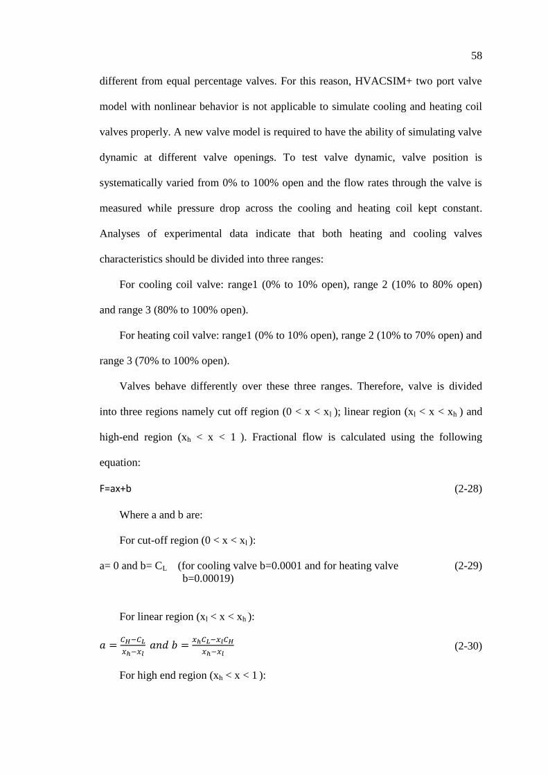
58

different from equal percentage valves. For this reason, HVACSIM+ two port valve

model with nonlinear behavior is not applicable to simulate cooling and heating coil

valves properly. A new valve model is required to have the ability of simulating valve

dynamic at different valve openings. To test valve dynamic, valve position is

systematically varied from 0% to 100% open and the flow rates through the valve is

measured while pressure drop across the cooling and heating coil kept constant.

Analyses of experimental data indicate that both heating and cooling valves

characteristics should be divided into three ranges:

For cooling coil valve: range1 (0% to 10% open), range 2 (10% to 80% open)

and range 3 (80% to 100% open).

For heating coil valve: range1 (0% to 10% open), range 2 (10% to 70% open) and

range 3 (70% to 100% open).

Valves behave differently over these three ranges. Therefore, valve is divided

into three regions namely cut off region (0 < x < xl ); linear region (xl < x < xh ) and

high-end region (xh < x < 1 ). Fractional flow is calculated using the following

equation:

F=ax+b (2-28)

Where a and b are:

For cut-off region (0 < x < xl ):

a= 0 and b= CL (for cooling valve b=0.0001 and for heating valve

b=0.00019)

(2-29)

For linear region (xl < x < xh ):

𝑎 =𝐶𝐻−𝐶𝐿

𝑥ℎ−𝑥𝑙 𝑎𝑛𝑑 𝑏 =

𝑥ℎ𝐶𝐿−𝑥𝑙𝐶𝐻

𝑥ℎ−𝑥𝑙 (2-30)

For high end region (xh < x < 1 ):

59

𝑎 =1−𝐶𝐻

1−𝑥ℎ 𝑎𝑛𝑑 𝑏 =

𝐶𝐻−𝑥ℎ

1−𝑥ℎ (2-31)

CL and CH are parameters representing fractional flow rate corresponding to valve

positions at xl and xh respectively. As Figure 2-9 demonstrate for cooling valve CL =

0.0001 and CH = 0.9834 and based on Figure 2-10 for heating valve CL = 0.00019 and

CH = 0.9703

Experimental data are used to estimate unknown parameters in the new valve

model. Eqs. (2-25) to (2-27) are combined to obtain the following model equation:

1

𝑊2 =1296

∆𝑃 𝐾𝑣2 (𝑎𝑥 + 𝑏)−2 +

𝑅𝑐𝑜𝑖𝑙

∆𝑃 (SI unit) or

1

𝑊2 =66.94

∆𝑃 𝐾𝑣2 (𝑎𝑥 + 𝑏)−2 +


∆𝑃 (IP unit)

(2-32)

This equation can be rewritten into the linear form:

𝑦 = 𝜃1∅1 + 𝜃2∅2 (2-33)

where y = 1

𝑊2 , ∅1 = (𝑎𝑥 + 𝑏)−2 , ∅2 = 1, 𝜃1 =1296

∆𝑃 𝐾𝑣2 and 𝜃2 =


∆𝑃. The

calculated values for fractional flow f form Eqs. (2-29)-(2-31) are used to calculate ∅1

at different regions and consequently applying least square method results in the

values of unknown parameters. Table 2-2 summarizes the parameters for heating and

cooling coil valves. Figure 2-9 & Figure 2-10 demonstrate the comparison between

simulated heating and cooling coil water flow rate at different valve positions and

corresponding experimentally measured values. Although, predicted flow rates by

model does not exactly match with experimental values but it is representing the best

fit model and yields to satisfactory results. The R2 for cooling coil valve model is 0.62

and for heating coil valve model is 0.84.

60

Table 2-2. Cooling and heating coil valves parameters estimated from experimental data

Parameters Explanation Value

Rcooling coil Cooling coil water flow resistance, 0.001 kg-m 90.18

KV-cooling coil Cooling coil valve capacity, m3/hr 0.93

CL-cooling coil Cooling coil valve leakage (fractional flow), % 0.0001

CH-cooling coil Cooling coil high-end fractional flow, % 0.9834

Rheating coil Heating coil water flow resistance, 0.001 kg-m 9584.4

KV-heating coil Heating coil valve capacity, m3/hr 0.45

CL-heating coil Heating coil valve leakage (fractional flow), % 0.0002

CH-heating coil Heating coil high-end fractional flow, % 0.9703

Figure 2-9. Experimental and simulated water flow rates vs. valve opening for cooling coil

61

Figure 2-10. Experimental and simulated water flow rates vs. valve opening for heating

coil

2.4 Boundary File Generation

The essence of HVACSIM+ simulation package can be found in MODSIM

which contains the solver of this package. In order to solve the system of governing

equations; it calls model definition file and boundary data files. Model definition file

contains structure of the model, physical and geometric characteristics of each

component, state variables initial value and state variables comprising time dependent

boundary variables. Therefore, the FCU model is influenced directly or indirectly by

both steady and time dependent factors that are included in the overall system

simulation: device performance parameters, zone interior loads, outdoor air

temperature and humidity, room and plenum temperatures, and inlet cooling and

heating water temperatures. The three types of controllable internal loads in each test

room are: lighting loads, sensible heat loads from people and false thermal loads

generated by the baseboard heaters. The values of these boundary conditions are

62

directly determined from the test facility measurements. Internal gain profiles are

provided to the model as time dependent boundary condition on the fractional basis

according to ERS schedule for various zones. Figure 2-11 is representing the actual

schedule of the internal gain profile. External gains consist of effective sol-air

temperatures based on ambient air temperature, solar flux and external wall properties

(DeSimone, 1996).

Figure 2-11. Fractional internal loads as time dependent boundary conditions

The ambient air physical properties and solar radiation effective on room heating

and cooling loads as well as internal heat gains are defined as time variant boundary

conditions.

2.5 Fault-free Model Validation

According to the literature there has been no prior work specifically about

dynamic simulation and validation of FCUs. As evidenced by the lack of any dynamic

model by which FCU performance can be simulated to generate data to assist further

63

research in their control and operation, as well as automatic fault detection and

diagnosis. The comprehensive FCU dynamic model developed here is validated by

comparing the data from simulated operation under fault-free condition with the

corresponding experimental data from ERS. Validation of the FCU model is

accomplished by a separate procedure at each of two levels: at the component level

and at the system level. The component level validation described in the previous

sections was accomplished to obtain the representative parameters of the

corresponding components. During model development, nominal parameters for FCU

performance within each TYPE were assigned only when suitable parameters from

manufacturer data were not available. Assignment of nominal parameters was

accomplished by an experimental procedure. Where manufacturer catalogs included

parameters for key components like fan, mixed air damper, heating and cooling coil,

component level validation was still conducted to ensure realistic model behavior.

Despite all of the efforts have been to validate the components accurately there are

some unavoidable uncertainty/error associated with measurement and data fitting.

Therefore, system level performance may not be in a very close agreement with

experimental data due to error propagation and problems with numerical stability and

convergence in the calculations. In this section the system level validation procedure

of fault-free dynamic simulation model for FCU is summarized.

2.5.1 Validation procedure

After component level validation to obtain FCU parameters, system level

validation is accomplished to evaluate the performance of the integrated components

all together. Furthermore, validation involves solving the right governing equations of

the system under simulation and comparing model predicted results against field or

64

experimental data. For FCU system level validation, dynamic behavior of the model is

validated by comparing simulation results with corresponding experimental data

generated by ERS. ERS has generated experimental data under fault-free operation of

FCUs interacting with exterior zones (east, west and south) for winter, summer and

fall seasons. Dynamic simulation using the FCU model unavoidably requires an

interacting zone model, including systemic interactions with the building’s


Parameters from the ASHRAE 1312 research project (Li et al., 2010) were used to


ambient conditions and adjacent zones.

Variables examined for system level validation included cooling and heating coil

valve positions, room air temperature, outdoor air damper position and hot water flow

rate. Although discharge (supply) and mixed air temperatures are measured in the test

facility, they are not used for validation due to very large experimental uncertainty

caused by uneven flow profiles around sensors. Thermal network validation as an

isolated superblock fed by supply air flow rate, outdoor air damper position, heating

and cooling coil valve positions from experimental data as well as corresponding time

dependent boundary condition raised this problem. The observations from thermal

network validation showed large disagreement between the model predicted supply

air and mixed air temperatures and the experimental ones (examined for couple days

in different seasons). Figure 2-12 (a-c) illustrates the result of isolated validation of

thermal network for a winter test day (Dec 22nd

2011). The corresponding control

signals and supply air flow rate are provided to the model from experimental data.

65

(a) East room FCU thermal network validation

(b) South room FCU thermal network validation

66

(c) West room FCU thermal network validation

Figure 2-12. FCU thermal network validation fed by control signals from experimental

data

In order to narrow down the problem, further analysis was accomplished focusing

on the coil model. Inlet air and water temperatures, inlet water and air flow rates were

provided to the model from experimental data. In Figure 2-13 the observations of

heating coil analysis on a winter test day (Jan 13th

2012) for east, south and west-

facing rooms are illustrated. This analysis was done for a couple of test days but we

suffice to illustrate the results of one day. As Figure 2-13 (a-c) demonstrates the

model predicted results for supply air temperatures do not match with experimental

data. The following evidences ended up to the conclusion that mixed and supply air

temperature sensor reading are unreliable:

1) For south room and partially east room mixed air temperature which is the

inlet air temperature of the heating coil is less than supply air temperature

while FCU is in heating mode.

2) For all rooms there is large discrepancy between heat transfer rate for water

side and air side for experimental data

67

(a) East room

(b) South room

68

(c) West room

Figure 2-13. FCU heating coil performance for east, south and west-facing rooms

Those weird observed evidences called for more analysis. In order to further

study this matter, the cases with no call for heating and cooling under the conditions

of 0% open and 100% open outdoor air damper (26th

& 29th

Oct 2011) underwent

investigation. Figure 2-14(a) illustrates comparison of supply, mixing and room air

temperatures for east and west- facing rooms and Figure 2-14(b) demonstrates those

temperatures comparison with ambient temperature for east, south and west-facing

rooms. The uncertainty associated with mixing air and supply air temperature sensor

can be clearly observed from the graphs. Especially Figure 2-14(b) illustrates uneven

temperature profile for supply and mixing air temperatures while they are expected to

be equal. In addition, the significant difference between ambient temperature and both

supply and mixing air temperatures imply to the uncertainty associated with those

temperature sensors.

69

(a) Comparison of supply, mixing and room air temperatures (outdoor air damper=0% open,

no call for heating and cooling)

(b) Comparison of supply, mixing, ambient and room air temperatures (outdoor air

damper=100% open, no call for heating and cooling)

Figure 2-14. Comparison of supply, mixing, ambient and room air temperatures with OA

damper=% open & 100% open

The mixed air temperature sensor located in the mixing chamber/box of FCU

does not reflect the well mixed temperature caused by mixture of fresh air and return

air due to the limited space of mixing chamber. The error/uncertainty in temperature

reading of mixed air propagates to supply air temperature profile too. In spite of

uneven supply air temperature profile alongside the FCU, its sensor reflects a local

point reading. All of these analyses and studies led us to ignore the mixed and supply

70

air temperatures for validation of FCU at system level. In the following sections the

results of normal validation are illustrated and discussed.

2.5.2 Fault –free model validation results

Validation of the FCU model under fault-free condition is accomplished by a

separate procedure at each of two levels: at the component level and at the system

level. During model development, nominal parameters for FCU performance within

each TYPE were assigned only when suitable parameters from manufacturer data

were not available. Assignment of nominal parameters was accomplished by an

experimental procedure. Where manufacturer catalogs included parameters for key

components like mixed air damper, heating and cooling coil, component level

validation was still conducted to ensure realistic model behavior. Although not

detailed here, dynamic simulation using the FCU model unavoidably requires an

interacting zone model, including systemic interactions with the building’s


Parameters from the ASHRAE 1312 research project (Li et al., 2010) were used to


ambient conditions and adjacent zones. Finally, dynamic behavior of the model is

validated by comparing simulation results with corresponding experimental data.

Variables examined for system level validation include cooling and heating coil valve

positions, room air temperature, outdoor air damper position and hot water flow rate.

Although discharge and mixed air temperatures are measured in the test facility, they

are not used for validation due to very large experimental uncertainty caused by

uneven flow profiles around sensors. Validation of FCU fault-free model has been

done on various days of three different seasons: fall, winter and summer. Figure 2-15

71

and Figure 2-16 show the simulation results comparison against experimental data on

a summer test day (July 30th

2011) and winter test day (January 8th

2012) for east,

south and west- facing rooms.

(a) East-facing room validation results

(b) South-facing room validation results

72

(c) West-facing room validation results

Figure 2-15. The results of FCU fault-free model validation in summer (07.30.2011)

In the presented graphs, the red line is representative of experimental data and

navy blue line is representative of simulation results. In summer operation, the

outdoor air minimum damper position is set to zero and the mixed air temperature set-

point is set to 100 F so that it is always closed. Fan mode is in “On” mode which

always runs at preset speed set at High during the normal test days, regardless the

cooling or heating PID output. As the heating coil valve position graph shows, there is

no need for heating and the FCU is operating in cooling mode in the depicted time

window. In the beginning of the simulation especially for east and west-facing rooms,

the cooling coil valve position tracks the value and trend of the experimental data but

as it gets closer to the evening the discrepancy between the two cases emerges. The

discrepancy between the simulated cooling coil valve position and the real position

arises from two factors. First, component tests for valve model validation were only

performed in the south facing room. Although ERS FCUs in the exterior rooms are

73

the same, there might be some differences that were neglected here. Secondly, the

simulated zone is more sensitive to changes in internal load and ambient air

fluctuations than the actual zone. The simulated room air temperature is representative

of well mixed air within the room, but in reality the room temperature sensor may

reflect a local temperature that is not necessarily reflective of a bulk room

temperature. For these reasons, the dynamics of the modeled FCU display some

deviation from the real FCU due in part to unavoidable simplifications to the zone

model that were necessary to keep the zone model tractable.

The performance of the developed model in predicting the dynamic variables for

FCU is evaluated using the R2 and RMSE defined in Eqs. (1-1) & (1-2)) and is

tabulated in Table 2-3.

Table 2-3. FCU model performance for summer test day (07.30.2011)

Variable R2 RMSE

Cooling coil valve

position

East Room 0.56 8.173

South Room 0.33 18.586

West Room 0.67 9.237

Room air temperature

East Room 0.65 0.75



To show the performance of the developed model in different weather condition a

winter test day ( 01.08.2012) is picked. Figure 2-16 demonstrates the simulation result

compare with the real one for this day.

74

(a) East-facing room validation results

75

(b) South-facing room validation results

(c) West-facing room validation results

Figure 2-16. The results of FCU fault-free model validation in winter (01.08.2012)

Validation of the FCU model for winter also demonstrates the same trend and led

to the same conclusion. As Figure 2-16 demonstrates as soon as turning off the

76

internal loads in 720-780 and 1020-1200 time frames; the modeled room calls for

heating while the real room either has lag or no call for heating. In addition, the room

model in TYPE 403 using 2C-3R model does not consider the solar beam radiation

transferred trough glazing. Considering the fact that ERS exterior rooms are

facilitated with large windows without any covering; the amount of solar radiation

transmitted to the room can’t be negligible. This evidenced the lag of the real room

response to the absence of internal load. Table 2-4 represents the performance of the

model for the winter test day.

Table 2-4. FCU model performance for winter test day (01.08.2012)

Variable R2 RMSE

Cooling coil valve

position




Heating coil valve

position

East Room 0.51 10.698


West Room 0.36 15.152

Room air temperature




2.6 Fault Model Development

Faults can be modeled in two different ways (Haves, 1997): 1) by changing




modeling a coil fouling fault by adding a new parameter that specifies the thermal

resistance of the deposit in a detailed coil model. In this study, faults are modeled by

77



allow the user to select a fault type and severity. The category of faults which may

occur in FCUs and the devices affected by these faults are listed in Table 2-5. The

FCU model simulates those faults with varying severity, which projects

proportionally to the fault symptoms observable in data. As Table 2-5 demonstrates,

various fault categories associated with FCU are listed in four different categories:

equipment, sensor, controlled devices and controllers. In the following sections a brief

review of various categories of potential faults for FCU and the type of faults which

are artificially implemented to different devices are described. Furthermore, the fault

flag arrangement imposing the fault type and severity to the simulation model is

discussed.

78

Table 2-5. FCU fault summary

Category Device Fault Name Fault Type

Summer

Test

Days

Fall

Test

Days

Winte

r Test

days

Equipment

Fan Failure Abrupt 1

Outlet Blockage Abrupt 1

Heating Coil Fouling-Airside Degradation 2

Fouling-Waterside Degradation 1

Cooling Coil Fouling-Airside Degradation 2

Fouling-Waterside Degradation 2

Filter Filter Restriction Degradation 1 1

Economizer

Restricted Airflow Opening

Blockage

1 1

Leaking OA/RA

DMPR Degradation

1 1

Sensor Room Temp Offset Degradation 2 2

MA Temp Offset Degradation 2 2

Controlled

Device

Heating Valve Stuck

Full Open 1

Full Closed 1

Partial Open 1

Leaking Degradation 1

Cooling Valve Stuck

Full Open 1

Full Closed 1

Partial Open 1

Leaking Degradation 1

OA/RA Damper Stuck

Full Open 1 1

Full Closed 1

Partial Open 1 1 1

Control

FCU Cycle I

Control Unstable Control Degradation

1 1

FCU Cycle II


1 1

FCU Cycle III


1 1

Heating Control Reverse Acting Implementation 1 1

Cooling Control Reverse Acting Implementation 1 1

2.6.1 Equipment Fault

The components of FCU may undergo faulty condition where faults could occur

in fan, coil (heating or cooling) filter and economizer. For fan, two types of faults,

namely, fan motor failure/ fan bearing seized and discharge outlet blockage are

modeled. Complete failure fault is modeled by outputting zero fan movement and

outlet blockage fault is modeled by adding a user specified bias to the simulated

pressure drop in FCU.

79

Two types of faults, namely, air side fouling and water side fouling are modeled

for coils. The studies in the literature shows that heat exchanger fouling can be

implemented by altering the heat-transfer coefficients (Bendapudi and Braun, 2002)

or the increase of thermal resistance can be represented by a fouling factor (House et

al.,1999). In this study, water side fouling fault in the experiment is imitated by

reducing the amount of hot or chilled water flow rate to a certain amount of total

water flow rate. Therefore the heat transfer coefficient or resistance does not change.

In the model it is replicated by increasing water flow pressure resistance of the coil by

a user specified value without affecting heat transfer coefficient. There is the same

situation for air side fouling; without manipulating air side heat transfer coefficient

the air flow pressure resistance is increased by a user specified value.

Filter fault is caused by depositing dirt and dust in it and results in more air

pressure drop passing through the filter. To replicate this fault in the model the air

flow pressure resistance is increased by a user specified value. Opening blockage of

outdoor air damper by debris, leaves etc. is the cause of restricted air flow fault for

economizer in equipment fault category which is replicated by increasing the pressure

resistance of the damper by a user specified value. Degradation of seating location of

mixed air damper caused its leakage and is modeled by adjusting a user specified

outdoor air flow rate when the damper is at fully closed position for outdoor air.

2.6.2 Sensor Fault

Offset fault for mixed air temperature and room air temperature sensor is

modeled by adding a user specified bias to the simulated sensor output, which is

achieved by Eq. (2-34)

𝑌𝑜𝑢𝑡𝑝𝑢𝑡 = 𝑌𝑖𝑛𝑝𝑢𝑡 + 𝐵𝑖 (2-34)

80

Where Youtput and Yinput are the output and input of sensor and Bi is user specified

bias which keeps constant with time.

2.6.3 Controlled Device Fault

Controlled device category includes mixed air damper and heating and cooling

valves faults. Two types of faults, namely, stuck fault and leaking fault are modeled

for valves and stuck fault is modeled for mixed air damper. Stuck fault which occurs

due to the actuator malfunction for both damper and valves is modeled by fixing the

simulated controlled device position to be a user specified position. Leaking fault

which is caused by wear and tear is modeled by adjusting a user specified flow rate

when the controlled device is 100% closed.

2.6.4 Controller Fault

Two types of control faults, namely, unstable control fault and reverse acting

control fault, are modeled in this study. Unstable control fault occurs when the PID

loops has not been tuned properly and the system is unstably controlled. This fault is

modeled by implementing a user specified proportional band for PID controllers. A

reverse acting actuator is a typical commissioning fault usually caused by incorrect

setting of the directional switch on the actuator. During this fault, the actuator follows

the control signal command reversely (i.e., the actuator closes down the heating valve

instead of opening it up).

2.6.1 Fault flag system

It is important to design a proper fault flag system that can be used by the users to

indicate fault selection and their associated severities. In this study, the fault model

implementation has been accomplished by designing a fault flag system in MODSIM

81

HEAD subroutine (Fortran 90). It is accessible to each TYPE of HVACSIM+ library

of components. In the designed fault flag system the category of fault is reflected by

the fault variable and the associated fault severity is determined by the fault severity

variable. The designed fault flag system for FCU has been summarized in Table 2-6.

In Table 2-6, the first column lists the four fault categories, which are equipment,

sensor, controlled device and controller faults. The second column lists the device or

process that would be affected by a fault. The third column summarizes the potential

fault status and fault type for a device or process. The fourth and fifth column list

variables used in MODSIM HEAD subroutine to store fault type and severity for each

device or process. The last column lists the TYPE in HVACSIM+ library of

component that would be affected by the faults associated with each device or

process.

82

Table 2-6. FCU fault flag system summary

Category Device Fault type Fault variable Fault severity

variable TYPE

Equipment

Fan 0- No fault, 1- Fan motor failure, 2-

Fan outlet blockage fan Vfan 307

Heating Coil

0- No fault, 1- Fouling Air-side, 2-

Fouling Water-side

coilfault(4) Vcoilfault(2,3) 314

Cooling Coil coilfault(3) Vcoilfault(2,3) 314

Filter 0- No fault, 1- Filter restriction filter Vfilter 307

Economizer 0- No fault, 1- Restricted air flow, 2-

leaking mixed air damper economizer Veconomizer 307

Sensor

Room air

temperature sensor 0- No fault; 1- Offset fault

RAtemp VRAtemp 311

Mixed air

temperature sensor MAtemp VMAtemp 311

Controlled

Device

Heating Valve 0- No fault, 1- Stuck, 2- leakage coilfault(2) Vcoilfault(1) 314

Cooling Valve 0- No fault, 1- Stuck, 2- leakage coilfault(1) Vcoilfault(1) 314

OA/RA Damper 0- No fault, 1- Stuck OAdamp VOAdamp 307

Controller

Heating coil control 0- No fault, 1- Unstable CONheat VCONheat 479

Cooling coil control 0- No fault, 1- Unstable CONcool VCONcool 479

Heating coil reverse

action 0- No fault, 1- Reverse CONheatreverse - 321

Cooling coil reverse

action 0- No fault, 1- Reverse CONcoolreverse - 321

2.7 Fault Model Validation

Given the simulation system model had been validated under fault-free

conditions, the only further validations required to ensure realistic representation of

faults were those on the altered parameter values. During the validation of fault

modeling, it is more important to compare fault symptoms rather than regenerating

83

the dynamics of each variable. This is due to the complex impacts of faults under real

world conditions, and the difficulty of simulating such impacts precisely. Therefore,

faulty operation validation does not need a comprehensive process as described for

fault free validation. In the following subsections the procedure of fault model

validation for FCU is described.


Both simulation results and experimental data are used to validate the modeling

of faults, involving simulation results under both faulty and fault-free conditions (to

identify simulated fault symptoms), and similarly for experimental real data (to

identify the real fault symptoms). The fault-free and faulty simulation results are

generated by adjusting fault flags. In order to ideally validate the system under faulty

condition; fault-free experimental data of a similar system running in parallel with the

faulty system is necessary. There is a lack of experimental data under fault-free

conditions for the same test day and exterior rooms undergoing the faulty test. Thus, a

normal test day with close or more severe weather condition (that is, a condition that

will cause system variables to change similarly as the tested fault) is picked as a

reference day to confirm that the system behavior and the observed symptoms in real

data are resulted from the fault and not the weather. As an example, for heating

reverse action fault in FCU on Jan 14th

a warmer fault-free test day can serve as

reference day. Comparison with a warmer test day helps to justify that the observed

symptoms are just due to the fault regardless of weather condition. As Figure 2-17

displays, Jan 8th

with a warmer weather condition is a candidate to be a reference day

for Jan 14th

. In Figure 2-17, the normal test day weather conditions are shown by solid

lines and the dotted line represents faulty test day weather conditions.

84

Figure 2-17. Weather comparison to pick a normal test day as reference day for heating

control reverse action fault in FCU

To assist validation of FCU fault model, experimental data under faulty

conditions (under different faults and severity levels) are collected from east and west

facing rooms in the ERS. Like fault-free tests, three test periods are scheduled during

summer, fall and winter for collecting faulty experimental data. Different faults are

implemented in different seasons because system operational characteristics and

control sequence change with weather conditions. Table 2-5 demonstrates the faulty

condition which has been tested in different seasons. The season operation has been

selected so that a specific fault yields measurable system difference compared with a

fault-free system. Since it is impractical to test all levels of severity for a degradation

fault only two or three levels of severity has been tested for each degradation fault.

Some faults have similar effects on the system during different seasons.

2.7.2 Fault model validation results

Validation of FCU fault model has been done on all faulty test days of three

different seasons: fall, winter and summer. For brevity a few fault cases from each

category is picked to demonstrate the symptoms associated with a certain fault and

85

defined severity. The following figures depict the comparison of simulation results

under faulty and fault-free conditions with the corresponding experimental

operational data. In the presented graphs, red and dashed navy blue lines are

representative of experimental data and simulation results, respectively, under the

faulty condition. In the same way, purple and dotted green lines are representative of

experimental data and simulation results under fault-free condition.

From the equipment category heating coil air-side fouling, cooling coil water-side

fouling as well as fan failure faults are picked to show the symptoms associated with

these faults. Figure 2-18 (a) demonstrates the fault model simulation results of FCU

with heating coil air-side fouling fault on a winter test day (Dec 24th

). Air side fouling

in the coils happens gradually due to the deposition of indoor dusts and other particles

included in indoor or outdoor air on the heat exchanger surfaces in contact with air.

Air side fouling of coils leads to increase in system pressure drop and,

correspondingly, decrease in heat transfer rate and eventually degrade system

performance. In the test site this phenomena is testing just by reducing fan speed

mimicking the decrease of supply air flow rate due to increase in pressure drop

followed by fouling while under normal condition fan speed is always at high. Thus

replicating this fault in the simulation is just by increasing the pressure resistance

without manipulating heat transfer coefficient of the coil. In order to emphasis the

symptoms associated with heating coil air-side fouling the closest normal test day is

selected (Jan 8th

). The symptoms associated with this fault are listed as the following:

1) Increase in cooling coil valve position. Heat transfer rate in water-side of

cooling coil increases by water flow rate elevation to compensate the decrease

of cold air flow rate due to the fouling.

86

2) Decrease in heating coil valve position and consequently hot water flow rate.

Due to this fault, air passages in heating coil are blocked which causes

increase in pressure drop and decrease in air flow rate. Air flow rate drops and

consequently the proportion of fresh cold air in the supply air decreases which

leads to decrease in heat transfer rate on both sides.

Figure 2-18 (b) demonstrates the fault model simulation results of FCU with

cooling coil water-side fouling fault on a summer test day (July 24th

). The water side

fouling is caused by deposition of mineral material of circulating water on the

surfaces of heat exchanger in contact with water. This phenomenon results in heat

exchanger performance degradation by reducing the overall heat transfer coefficients

and increasing the resistance to the fluid flow. In the experiment, water side fouling

faulty test is employed by restricting the maximum water flow rate through the coil by

50% and 25% to mimic the increase of resistance to water flow rate. Thus, heat

transfer coefficient of the coil does not change during the experiment. Replicating this

fault to the model is accomplished just by increasing water side pressure resistance

without manipulating heat transfer coefficient of the cooling coil. The closest normal

test day to serve as reference day is July 16th

. The symptoms associated with this fault

are listed as the following:

1 Increase in cooling coil valve position. Cooling water flow is restricted due to

this fault therefore its lack during the cooling mode operation of FCU is

compensated by increase in valve position.

2 Increase in room air temperature. Increase in cooling coil valve position in the

morning result in more chilled water flow rate which is adequate to keep room

temperature set point. But restricted chilled water flow rate shows its obvious

87

effect in the afternoon. Even fully opening of cooling coil valve does not result

in adequate water flow rate to keep room cooling temperature set point.

Figure 2-18 (c) depicts the fault model simulation results of FCU with fan failure

fault on a fall test day (Oct 21st). A cooler normal test day is selected to serve as

reference day (Oct 20th

). The symptoms associated with this fault are as the following:

1) Increase in cooling coil valve position. Cooling valve position elevation is the

results of decrease in forced convection heat transfer rate due to the fan

failure.

2) Room temperature floating. Even fully opening of the cooling coil valve is

unable to meet room cooling demand. Because the equipment in charge of

blowing the air through the coils is broken.

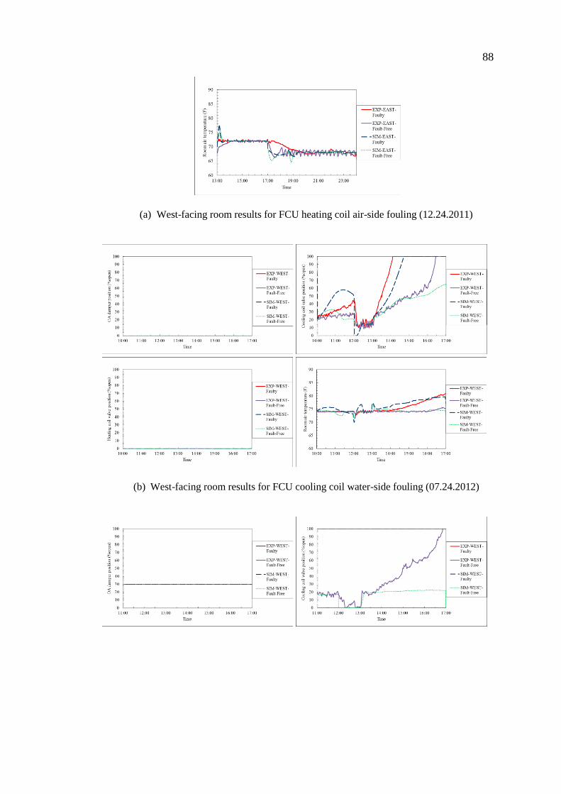
88

(a) West-facing room results for FCU heating coil air-side fouling (12.24.2011)

(b) West-facing room results for FCU cooling coil water-side fouling (07.24.2012)

89

(c) West-facing room results for FCU fan failure (10.21.2011)

Figure 2-18. Some examples of FCU equipment category fault

From sensor category the room temperature sensor bias fault is picked to show.

Figure 2-19 depicts the fault model simulation results of FCU with a +2◦F bias in

room temperature sensor reading on a winter test day (Jan 4th

). The closest normal test

day is selected to serve as reference day (Jan 8th

). The symptoms associated with this

fault are as the following:

Decrease in heating coil valve position and hot water flow rate. Room

temperature sensor reading is passed to the controller to keep room

temperature by adjusting heating and cooling coil valve positions. Room

temperature sensor bias causes artificial decrease in the room heating load

and heating coil load decreases accordingly.

Decrease in the room temperature by 2◦F. The dashed navy blue line is

representing the room temperature (result of thermal superblock) while the

light blue one is representing sensor reading (result of sensor superblock)

under faulty condition. The simulated room temperature under the faulty

condition is 2◦F less than the temperature sensor reading.

90

Figure 2-19. East-facing room results for FCU room temperature sensor bias (+2◦F)

(01.04.2012)

Form the controlled device category fault, heating coil valve stuck at fully open

position and leakage as well as cooling coil valve stuck at partially open position are

picked to show the symptoms associated with each fault. Those fault occurs as the

result of actuator malfunctioning. Figure 2-20 (a) demonstrates the fault model

simulation results of FCU with heating coil valve stuck at fully open position on a

winter test day (Jan 10th

). The closest normal test day is selected to serve as reference

day (Jan 8th

). Figure 2-20 (b) displays the fault model simulation results of FCU with

heating coil valve leakage fault on a winter test day (Jan 12th

). This fault occurs when

91

the valve signal is totally closed but due to its wear and tear, valve is unable to block

water flow rate through the coil. A warmer normal test day is selected to serve as

reference day (Dec 22nd

).The symptoms of these two faults can be readily

distinguished by noticing:

1) The contradiction of heating coil valve position and heating water flow rate.

While the controller is sending a signal for the heating coil valve to be closed, the

heating water flow rate is at the maximum level for the fully open stuck valve and at

0.5 GPM for leaking valve fault.

2) The heating coil valve position at 0% open on a cold winter evening.

According to the fault-free experimental data, the west-facing room calls for heating.

The same behavior is displayed in the simulation result for a fault-free condition.

3) The cooling coil valve position on a cold winter evening. Under the faulty

condition on a winter night, the zone calls for cooling in both the experiment and

simulation cases due to the hot supply air, which is caused by excess hot water flow

rate through the heating coil.

4) The room temperature maintained at cooling setpoint. For the faulty situation

the FCU is operating in cooling mode, so room temperature is kept near the cooling

setpoint, while for the fault-free condition it is fluctuating around the heating setpoint.

Figure 2-20 (c) demonstrates the fault model simulation results of FCU with

cooling coil valve stuck at partially open position on a summer test day (July 28th

).

The closest normal test day to serve as reference day is Aug 9th

. The symptoms

associated with this fault can be readily distinguished by noticing:

1) The cooling coil valve position at 0% open on a hot summer day. According

to the fault-free experimental data, the west-facing room calls for cooling.

92

The same behavior is displayed in the simulation result for a fault-free

condition.

2) The heating coil valve position on a hot summer day. Under the faulty

condition, the zone calls for heating in both the experiment and simulation

cases due to the extremely cold supply air, which is caused by excess chilled

water flow rate through the cooling coil.

3) The room temperature maintained at heating setpoint. For the faulty situation

the FCU is operating in heating mode, so room temperature is kept near the

heating setpoint, while for the fault-free condition it is fluctuating around the

cooling setpoint.

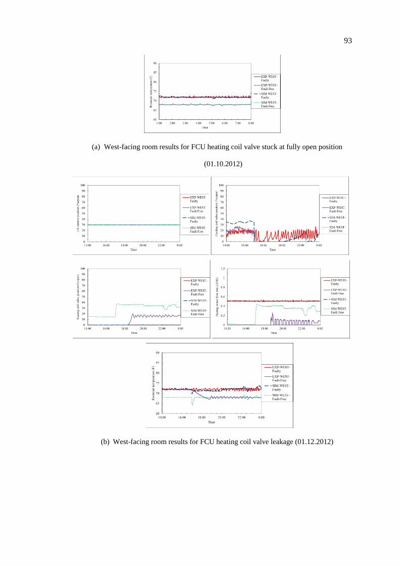
93

(a) West-facing room results for FCU heating coil valve stuck at fully open position

(01.10.2012)

(b) West-facing room results for FCU heating coil valve leakage (01.12.2012)

94

(b) West-facing room results for FCU cooling coil valve stuck at partially open position

(07.28.2011)

Figure 2-20. Some examples of FCU equipment category fault

To illustrate a fault case for control category, reversed action of heating coil in an

east-facing zone on a winter evening (Jan 14th

) is selected. A reverse-acting actuator

is a typical commissioning fault usually caused by incorrect setting of the directional

switch on the actuator. During this fault, the actuator follows the control signal

command reversely (i.e., the actuator closes down the heating valve instead of

opening it up). A warmer normal test day would cause the system variables to behave

95

similarly to the fault, so this is chosen as a reference day (Jan 8th

). The symptoms of

the heating coil reverse acting fault can be readily distinguished by noticing:

1) The contradiction of heating coil valve position and heating water flow rate.

While the controller is sending a signal for the heating coil valve to be closed, the

heating water flow rate is at the maximum level.

2) The heating coil valve position at 0% open on a cold winter evening (below

30F). According to the fault-free experimental data, the east-facing room on a warmer

normal day calls for heating. The same behavior is displayed in the simulation result

for a fault-free condition.

3) The cooling coil valve position on a cold winter evening (below 30F). Under

the faulty condition on a winter evening, the zone calls for cooling in both the

experiment and simulation cases due to the extremely hot supply air, which is caused

by excess hot water flow rate through the heating coil.

4) The room temperature maintained at cooling setpoint. For the faulty situation

the FCU is operating in cooling mode, so room temperature is kept near the cooling

setpoint, while for the fault-free condition it is fluctuating around the heating setpoint.

96

Figure 2-21 .East-facing room results for FCU heating control reverse action (01.14.2012)

2.8 Conclusion and Summary

A validated, dynamic numerical model of a FCU has been developed as a single

integrated component for inclusion in the component library of the HVACSIM+

simulation package by adding three new TYPEs to that library. The structure of the

FCU model and the justification for using the HVACSIM+ package in particular have

been discussed. Validation of the FCU model started with component level validation,

followed by validation of the model “installed” within an overall system. Experiments

were conducted to investigate and determine key model parameters. Real operational

data provided by ERS served as a reference to which simulation results were

compared. Under fault-free conditions, the FCU model agreed well with reference

data for several days in different seasons (summer, fall and winter). A fault flag

system gives the model the flexibility to simulate various faults modes with differing

97

severities without the need to develop additional TYPEs. That the model underwent a

comprehensive fault matrix and validated well against experimental data establishes

its validity to serve as a tool for evaluating FCU fault detection and diagnostic

methods.

98

3. CHAPTER THREE: DUAL DUCT DOUBLE FAN SYSTEM DYNAMIC MODEL DEVELOPMENT IN HVACSIM+ AND VALIDATION- FAULTY AND FAULT

FREE

3.1 Introduction

In a dual duct system, hot and cold air flows are separately carried by two parallel

duct systems. The hot deck is equipped with a heating coil and the cold deck is

equipped with a cooling coil. The two decks run in a parallel configuration throughout

the building. In a terminal unit, the proper proportions of hot and cold air streams are

modulated by cold air and hot air dampers before proceeding downstream to the

space. The simultaneous availability of hot and cold air enriches the flexibility of this

system to handle zones with widely varying loads. Meanwhile, energy could be saved

by utilizing outside air directly as hot air or cold air in different seasons. The dual

duct systems may be designed as constant air volume (CAV) or variable air volume

(VAV). In a CAV dual duct system, the supply air flow rate through the supply fan

and to each zone is constant. However, the flow rates through the cold and hot decks

vary depending on the requirements to satisfy the individual zone load. In a VAV dual

duct system, the supply air flow rate through the supply fan is not constant and is

dependent on the zone temperature control and ventilation needs. Similar to single

duct VAV terminal units, VAV dual duct terminal units can also be categorized as

pressure-dependent or pressure-independent units. A pressure-dependent VAV control

scheme uses the space temperature sensor to directly control the position of the

modulating devices. The actual airflow delivered to the space is a by-product of this

position and depends on the duct system static pressure at the inlet of the terminal

unit. Although the space temperature sensor will continually correct the position of

the modulating device, the response can be sluggish and cause unacceptable

temperature variations within the space. In contrast, a pressure-independent VAV

99

control scheme directly controls the actual volume of primary air that flows to the

space (Kreider et al. 2002). An airflow-measuring device on the terminal unit makes

this possible. The position of the modulation device is not directly controlled and is

basically a by-product of regulating the airflow through the unit. Because the airflow

delivered to the space is directly controlled, it is independent of inlet static pressure.

Pressure-independent control increases the stability of airflow control, and allows

minimum and maximum airflow settings to become actual airflows rather than

physical positions of the modulation device. It is clearly the most popular form of

VAV terminal unit control. More details about how dual duct systems are controlled

can be found in (Kreider et al. 2002).

Over the past three decades, various computer software applications have been

developed to simulate dynamic interactions between a building’s envelope, its internal

loads, its ambient conditions, and its HVAC systems, but very little attention has been

devoted to dual duct systems. Salsbury et al. (2000) discussed the potential of

simulation as a performance validation tool to evaluate a dual duct single fan system

installed in an office in San Francisco. But there has been no prior work specifically

about dynamic simulation and model validation for dual duct systems. The

development of advanced control, operation, and automated fault detection and

diagnosis techniques requires reliable simulation tools, therefore there is a need to

develop a simulation tool that is capable of simulating realistic fault free and faulty

operational data for dual duct systems.

The work documented here models a pressure-independent VAV dual duct

double fan system serving four zones -vary in orientation- to be run within the

HVACSIM+ dynamic simulation software package. Dynamic simulation of dual duct

system presents unique challenges whish are addressed in this chapter. The developed

100

model not only opens ways to synthesize operational data under fault-free conditions,

but also makes it possible to predict the symptoms associated with various faulty

conditions and their effects on the system performance and occupant comfort. A

comprehensive and systematic validation procedure, using data collected

experimentally from real dual duct system at ERS laboratory, is used to validate the

tool under both faulty and fault-free operating conditions in three different seasons.

The validated tool not only predicts real-world dual duct system behavior under

different control strategies, but it also predicts symptoms associated with various

faults, as well as the effects those faults have on system performance at various

severities. This chapter describes the challenges during the air flow network

development and the way to tackle them. It also express the procedure of model

development from the new added TYPEs to HVACSIM+ library of components to

validation of the model at both component and system levels. It also spends on fault

modeling by designing fault flag and validation of fault model.

3.2 Test Facility and Experimental Set up

Experiments have been conducted at Iowa Energy Center Energy Resource

Station (ERS) on a full scale dual duct system in three different seasons to generate

operational data used in validation of the developed model for this study. The ERS

has been described in at least three earlier studies (Norford et al. 2000, Castro et al.

2003, Li et al. 2010). The major feature of this test facility is two identical HVAC

systems (A and B systems). However, significant modifications have been made to

the two identical single duct AHU systems (AHU-A and B) to convert them from two

101

single duct systems as previously described to one dual duct double fan system with

one return duct.

More specifically, the following major changes have been made: 1) The two

existing and identical single duct AHUs (AHU-A and B) were connected by a duct

(bridge), so that the mixing box and return duct of the AHU-B were used as the dual

duct mixing box and return duct; 2) In AHU-A, the duct work before the bridge

connection was completely blocked. The downstream (after the connecting bridge)

components of AHU-A, including a heating coil, a cooling coil (not used), and a

supply fan, were used in the dual duct system; 3) In the four test rooms that were used

in this study, pressure independent dual duct terminal units were installed. After these

changes, AHU-A and B were respectively serving as the hot deck and cold deck of the

new dual duct system. Instrumentation used in this study consisted of humidity,

pressure, temperature and air flow sensors as well as electric power meters to monitor

the system. Figure 3-1 demonstrates the new dual duct double fan system and the four

test rooms including: west A, south A & B and east B.

ERS has provided operational data under a wide variety of fault-free and faulty

operational conditions in three different seasons: summer, fall and winter. To generate

dual duct system operational data under normal conditions all rooms were operated

without imposed faults. To establish data under faulty conditions, the east B, south A

and west A-facing rooms were operated with deliberately imposed faults while the

102

south B room ran normally. The zones have identical construction and details about

the zone envelop structure are provided by Price and Smith (2003).

Figure 3-1. Schematic of dual duct double fan system at ERS serving four perimeter zones

The speed of supply fans are modulated to maintain each deck static pressure at

the static pressure setpoint, which is generally at 1.6 in. W.G. Two PI control

algorithms are used to control the speed of cold and hot deck supply fans. The control

sequence used to control the return fan is air flow rate matching, the summation of

airflow rate from hot and cold decks. In the summer the economizer mode is disabled

and the minimum requirement for outdoor air damper opening is 0% while in the

winter and fall economizer is enabled and the minimum requirement for outdoor air

103

damper opening is 45%. Therefore, in the summer cold deck supply air temperature is

maintained at the set point just by mechanical cooling or control of cooling coil valve.

But in the winter and fall the control sequence used to maintain cold deck supply air

temperature at the setpoint is divided into three control regions, namely, mechanical

cooling, mechanical and economizer cooling and economizer cooling as shown in

Figure 3-2. Each region depends on whether or not outdoor air temperature is greater

or less than a reference temperature known as the economizer temperature setpoint

(60F), and whether the cold deck supply air temperature is above or below setpoint.

The regions correspond to the output from a single PI control algorithm that is

split into the control of outdoor air damper and cooling coil valve. The PI control

algorithm has an output that ranges from 0 to 200. During the mechanical and

mechanical and economizer cooling modes, the output from the PI control algorithm

ranges from 100 to 200, corresponding to a cooling coil position from 0 to 100 %

open. The outdoor air damper is held in the minimum position (mechanical cooling

only) when outdoor air temperature is above economizer setpoint. The outdoor air

damper is fully open (mechanical and economizer cooling) when outdoor air

temperature is less than economizer setpoint and when the output of PI is larger than

100. As outdoor air temperature drops, the need for mechanical cooling is eliminated

(output from the PI control algorithm drops below 100) thereby switching the control

sequence to the economizer cooling mode. In this mode, cold deck supply air

temperature is maintained by modulating the outdoor air damper. The output from the

PI control algorithm ranges from 0 to 100, corresponding to the outdoor air damper

position ranges from the minimum requirement to 100 % open.

During this project, AHU-A provides 90°F supply air as the hot deck, and AHU-

B provides 55°F as the cold deck to the four dual duct mixing boxes. All four test

104

rooms (EB, SA, SB, and WA) are equipped with the identical model dual-duct mixing

box. The room temperature setpoint for the four test rooms is constant during the test

and is 68°F for heating setpoint and 72°F for cooling setpoint.

Figure 3-2. Cold deck supply air temperature control sequence

The dual-duct terminal unit mixes air from the hot and cold deck supply inlets in

order to maintain the space temperature in the test room. The dampers modulate from

a minimum CFM setpoint of 100 CFM for both the cold and hot decks, to a maximum

CFM setpoint of 1000 and 400 CFM for the cold and hot deck respectively. Each dual

duct box terminal unit is controlled by a Johnson Controls VMA-1420 controller to

implement the control sequence. The VMA controller determines the flow setpoint for

each deck, which is compared to the actual flow rate that is measured via a differential

pressure sensor for each deck. The controller modulates the damper open and close in

order to achieve the setpoint. Figure 3-3 shows the dual duct terminal unit control

105

diagram. Since the implemented control sequence by Johnson Control is a patented

one, a similar control sequence from Carrier is selected as a substitute.

Figure 3-3. Dual duct terminal unit control diagram

On a call for cooling, the hot deck damper will remain at its minimum position

(for 100 CFM) and the cold deck damper will modulate open in order to satisfy the

space temperature setpoint. As the space load decreases the cold deck damper will

gradually close until it reaches its minimum position (for 100 CFM). On a call for

heating, the cold deck damper will remain at its minimum position and the hot deck

damper will modulate open to satisfy the room temperature setpoint.

3.3 Fault-Free Dynamic Model Development

In order to model dual duct system properly in HVACSIM+, all of the

constitutive processes represented by the model are divided among different

superblocks. Each superblock represents one category of process states associated

with the system that is both physically and numerically independent from- or at most,

coupled only weakly to- any other category of the process states in the system. In the

case of the dual duct system, five distinct categories of states—(1) sensors, (2)

actuators, (3) control logic, (4) fluid (i.e., mass flow and pressure), and (5) thermal

106

(temperature and humidity)—are each modeled by a dedicated superblock/network.

Especially for a large system like dual duct containing various components; breaking

the system down into the constituent independent subsystems helps to reduce time

intensity of the simulation. This section presents the subsystem structures of a dual

duct system in HVACSIM+, the constituent TYPEs of each superblock and the

required TYPEs which should be added to the HVACSIM+ library of components to

model dual duct system. Furthermore, the special challenges to model air flow

network of dual duct system are described. In addition, the process of determining the

parameters of key/new components in the air flow and thermal networks are

described.

3.3.1 Dual duct double fan system structure in HVACSIM+

The representative components (TYPEs) of each state category in dual duct

system are grouped as a network to create a single superblock/network. Each

superblock is an independent subsystem within which the system of governing

equations of one state category is solved simultaneously. In the air flow superblock

mass-pressure equations are solved simultaneously independent from other process

states constituent of dual duct system. Figure 3-4 shows air flow network

configuration of ERS dual duct system with double fans.

107

Figure 3-4. Dual duct system air flow network configuration

In this Figure, each box represents an UNIT to which a TYPE has been assigned.

The description and the TYPE that each UNIT uses have been provided within the

UNIT box. The inputs and outputs of each UNIT have also been specified. In Figure

3-4, mass flow rates, pressures, and control signals are respectively presented by m, p

and C.

Similarly the constitutive components of dual duct system thermal state are

grouped to create thermal network as an independent superblock/ network. Figure 3-5

demonstrates the thermal network configuration of ERS dual duct system with double

fans. Like air flow superblock, each unit is representative of a component described

by a TYPE containing the governing equations of each component thermal state. In

Figure 3-5, temperature, humilities, and heat transfer rates are respectively presented

by T, H and Q.

All of the control signal inputs are provided by control superblock. Figure 3-6

shows the control network of dual duct system comprising the control signals passed

to different superblocks.

108

Figure 3-5. Dual duct system thermal network configuration

Figure 3-6. Dual duct system control network configuration

109

3.3.1.1 New TYPEs added to HVACSIM+ to model dual duct double fan system

Most of the TYPEs that have been used in this dual duct air flow network (Figure

3-4) are the existing TYPEs provided by the HVACSIM+ component library and have

been used in previous studies. Three new TYPEs, i.e., TYPEs 535, 536 and 538 have

been developed to simulate the air flow rate and pressure in dual duct terminal units.

TYPE 535 determines hot, cold, and total air flow rates at the two inlets and one

outlet, when pressures at these inlets and outlet are given. TYPE 536 determines air

flow rate for hot deck inlet, total air flow rate for outlet, and cold deck inlet pressure,

when hot deck inlet pressure, outlet pressure, and cold deck inlet air flow rate are

given. Similarly, TYPE 538 determines air flow rate for cold deck inlet, total air flow

rate for outlet, and hot deck inlet pressure, when cold deck inlet pressure, outlet

pressure, and hot deck inlet air flow rate are given. These different TYPEs are used

for different test room configurations. Dominant equations of TYPE 535, which is

used as dual duct terminal unit for south B room (refer to Figure 3-4), are presented in

Eqs. (3-1) to (3-3).

𝑚8 = √𝑃13 − 𝑃23

𝑅ℎ𝑜𝑡 𝑑𝑎𝑚𝑝𝑒𝑟

(3-1)

𝑚16 = √𝑃21 − 𝑃23

𝑅𝑐𝑜𝑙𝑑 𝑑𝑎𝑚𝑝𝑒𝑟 (3-2)

𝑚18 = 𝑚8 + 𝑚16 (3-3)

m8, m16 and m18 as well as P13, P21 and P23 have been illustrated in Figure 3-4.

Furthermore, Rhot damper and Rcold damper are the pressure resistances of hot and cold

dampers, respectively. The required parameters including the duct and damper

pressure resistance determination is described in section 3.3.2. The governing

equations of TYPE 536 and 538 are similar. For example, the dominant equations for

110

TYPE 536, which is used as terminal unit for West-A room, are presented in Eqs.

(3-4) to (3-6).

𝑚6 = √𝑃11 − 𝑃22

𝑅ℎ𝑜𝑡 𝑑𝑎𝑚𝑝𝑒𝑟

(3-4)

𝑃20 = 𝑃22 + 𝑅𝑐𝑜𝑙𝑑 𝑑𝑎𝑚𝑝𝑒𝑟𝑚152

(3-5)

𝑚17 = 𝑚6 + 𝑚15 (3-6)


Equations for TYPE 538 are not presented here for brevity.

all of the TYPEs that have been used in dual duct thermal network (Figure 3-5)

are the existing TYPEs provided by the HVACSIM+ component library and have

been used in previous studies. In order to control the dual duct terminal units, a new

TYPE has also been added to HVACSIM+ library (Figure 3-6). TYPE 477 is

representing the Carrier dual duct terminal units with control strategy close to ERS

dual duct terminal units. Carrier control sequence for dual duct terminal units can be

found in APPENDIX C.

3.3.1.2 Special Challenges in the simulation of dual duct systems

In comparison with single duct systems, dual duct systems present unique

challenges, especially regarding air flow simulations. Because the dual duct air flow

network has two separate air flow paths (hot and cold) that are strongly coupled, it is

subject to convergence issues. Therefore, how to simulate them simultaneously and

robustly is a key obstacle. Here, the focus is to model the constituent components of a

dual duct system in terms of their governing equations, as well as the arrangement of

these equations to achieve a stable and efficient simulation. The arrangement of

UNITs as well as the equation formats within a UNIT need to be carefully considered

111

to avoid convergence problems. Different UNIT arrangements and equations formats

were tried and discarded before those shown in Figure 3-4 were found effective. One

unique TYPE specifically used for the dual duct air flow network is the main duct

splitter unit TYPE 345. The equations used in this TYPE are summarized here:

𝑚4 =𝑅𝐻𝐷𝑚2 ∓ √𝑅𝐻𝐷 𝑅𝐶𝐷 𝑚2

2 − (𝑅𝐻𝐷 − 𝑅𝐶𝐷)(𝑃4 − 𝑃5)

(𝑅𝐻𝐷 − 𝑅𝐶𝐷)

(3-7)

𝑚3 = 𝑚2 − 𝑚4 (3-8)

𝑃3 = 𝑃4 + 𝑅𝐻𝐷m32 − 𝑅𝑖𝑛𝑙𝑒𝑡m2

2 (3-9)


Furthermore, RHD, RCD and Rinlet are the pressure resistances of the junction dividing

the flow between hot and cold decks.

The TYPE 345 splitter equations are different from those of TYPE 346,

commonly used in single duct simulations. For comparison, the equations for TYPE

346 are provided as Eqs. (3-10) to (3-12).

mmain outlet = minlet − mbranch (3-10)

𝑃𝑖𝑛𝑙𝑒𝑡 = 𝑃𝑚𝑎𝑖𝑛 𝑜𝑢𝑡𝑙𝑒𝑡 + 𝑅𝑚𝑎𝑖𝑛 𝑜𝑢𝑡𝑙𝑒𝑡m𝑚𝑎𝑖𝑛 𝑜𝑢𝑡𝑙𝑒𝑡2 + 𝑅𝑖𝑛𝑙𝑒𝑡minlet

2 (3-11)

𝑃branch = 𝑃𝑚𝑎𝑖𝑛 𝑜𝑢𝑡𝑙𝑒𝑡 + 𝑅𝑚𝑎𝑖𝑛 𝑜𝑢𝑡𝑙𝑒𝑡m𝑚𝑎𝑖𝑛 𝑜𝑢𝑡𝑙𝑒𝑡2 − 𝑅𝑏𝑟𝑎𝑛𝑐ℎmbranch

2 (3-12)

Considering the first splitter after the supply fan in the hot deck (the top deck)

minlet and Pinlet are m3 and P7, mmain outlet and Pmain outlet are m5 and P10 and mbranch and

Pbranch are m6 and P11. Parameters Rinlet, Rmain outlet and Rbranch are the respective

pressure resistances. The use of TYPE 345 as the main duct splitter was found to be

critical to receive robust and converging performance of dual duct air flow network

simulations.

112

3.3.2 Model parameters

For each UNIT of every superblock, the values for the parameters need to be

determined. Therefore, there are too many parameters need to be determined for

simulation to represent the dual duct double fan system at the test facility. Many of

the components in this dual duct system, such as the mixing box, heating/cooling

coils, hot and cold deck supply fans and the return fan are the same components used

in the ASHRAE 1312 research project (Li, et al., 2010). Therefore, some parameters

obtained from ASHRAE 1312 project are kept the same for these components. Some

other parameters are determined through a designed experiment especially for the

critical and new components like hot and cold deck dampers in the terminal units and

heating and cooling coil valves. Therefore, at this point component level validation is

accomplished for those key components to determine their representative parameters.

In the following the parameter determination procedure for different components in

the air flow and thermal network are discussed in detail.

3.3.2.1 Air flow network parameters determination

In the modelling of air flow network, duct work pressure resistances and fan

performance curve are of significance and need to undergo component validation. As

mentioned earlier, other than the modifications to the duct work of AHU-A & B, to

convert them to a dual duct double fan system, VAV boxes are replaced by four new

terminal units. Therefore, duct work pressure resistances especially in the modified

junctions and also dual duct terminal unit dampers model parameters need to be

determined. ERS run component test for hot and cold dampers in the terminal unit of

south B room to provide data to determine their required parameters. The procedure

of determining parameters for the modified junctions and terminal unit dampers are

described in sections 3.3.2.1.1 and 3.3.2.1.2 respectively. Furthermore, significant

113

differences were found between the fan data generated from the ASHRAE 1312

project and this study. Therefore, new parameters are generated for supply fans and

return fan which are discussed in section 3.3.2.1.3. APPENDIX D provides a detailed

table that summarizes all parameters needed for the dual duct simulation and their

values based on the ERS system.

3.3.2.1.1 Pressure resistance of modified junctions in supply and return ducts

In this project, which uses explicit method, the relationship between mass flow

rate and corresponding pressure drop for a straight duct (TYPE 341), a flow split

junction (TYPE 345 & 346), and a flow merge junction (TYPE 348) is modeled using

the flow resistance model as expressed in Eq. (3-13):

ΔP = R𝑇w2 (3-13)

where ΔP is the pressure drop, w is the mass flow rate, and RT is the air flow

resistance. One parameter, namely, the flow resistance for the straight duct RT, needs

to be determined for each straight duct. One flow split model (TYPE 345) for main

duct and three flow split models (Type 346) before the first three zones are used to

model the flow split junctions. Each flow split junction is characterized by three

pressure resistances. The flow split model incorporates pressure resistances for the

fitting and the straight ducts connecting with it. Three flow merge models (Type 348)

are used in the return duct to model the flow merge junctions for the zones. Similar to

the flow split model, flow merge model also includes three flow resistances which

incorporate the pressure resistances for both fitting and straight ducts connected to the

fitting.

To determine the flow resistance parameter needed in a straight duct model, the

friction loss for a typical galvanized steel duct is determined first based on the duct

114

size and design air flow rate (ASHRAEb, 2001). Eq. (3-13) is then used to calculate

the flow resistance RT based on the design air flow rate (w) and corresponding friction

loss (P).

For a flow split or flow merge model, the friction loss coefficient for the junction

is firstly determined based on the junction size and its design air flow rate (Pita,

2002). The pressure drop for a flow split or merge junction at the design air flow rate

is then calculated based on the friction loss coefficient (Pita, 2002):

ΔP = C ∗ (𝑉

4000)2 (3-14)

where C is the loss coefficient, and V is the design air velocity (ft/min). Based on

the design air flow rate and pressure drop, the flow resistance for the converging or

diverging junctions in supply and return ducts are calculated using Eq. (3-13). Notice

that the three flow resistances used in the flow split or merge models also include the

straight ducts connected to the fitting. Detailed calculation information is summarized

in APPENDIX E.

3.3.2.1.2 Pressure resistance of hot and cold dampers in dual duct terminal units

Since dual duct terminal units are new components in the modified AHUs at

ERS, a new component test was performed in south B room for its hot and cold

dampers. During damper component testing, damper positions were systematically

adjusted from 0% to 100% open with 10% increments for cold and hot dampers in the

south B room dual duct terminal unit. The pressure drop across the dampers and

resulting discharge air flow rate were measured after the system reached steady state.

Experimental data generated from this component test are then used to determine hot

and cold dampers’ loss coefficient (𝐾𝜃) and then pressure resistances at various

damper positions. The pressure drop across the dampers is calculated by Eq. (2-5).

115

As Eq. (2-5) shows 𝑙𝑜𝑔𝑒𝐾𝜃 is a function of damper position. Various models

considering linear region covering various ranges of 𝜃 (damper opening) were fitted

to the experimental data points using the three region model approach for 𝑙𝑜𝑔𝑒𝐾𝜃

versus damper position (refer to Eqs.(2-6)- (2-8)). The changes between different

models (in Figure 3-7) included starting and ending damper positions for each region

and/or model parameters. The goal was to develop a model with good overall R2 and

also small modeling error between 50 and 60% damper positions. As Figure 3-7

demonstrates that approach was unable to fit a model with proper coverage for all data

points especially for damper opening between 50 and 60 % which is very commonly

used damper position range (according to the experimental data examination).

Therefore different approach, least square method, is used to fit a polynomial model

which is the best model to the experimental data points. As Figure 3-8 depicts the

polynomial model represents component test data point with close agreement

covering for the whole range of damper opening.

116

Figure 3-7. Hot (top) and cold (bottom) damper models (using three region approach) in

dual duct terminal unit

Figure 3-8. Hot (left) and cold (right) damper models (using least square method) in dual

duct terminal unit

117

3.3.2.1.3 Coefficient of fans (hot and cold deck supply fan and return fan)

Although the supply fans used in this dual duct system are the same as the ones

(AHU-A and -B) used in the ASHRAE 1312 project, significant differences were

found between the fan data generated from the ASHRAE 1312 project and this study,

mostly due to the duct work modifications and different operating conditions.

Therefore, new parameters are generated from experimental data collected under

normal operation for the two supply fans. The procedures used in determining the new

fan parameters are similar to those described in the previous chapter and ASHRAE

RP1312 project and not repeated here.

Therefore, new parameters are generated from experimental data (June 9th

2013

and Oct 3rd

2013 for cold deck and Nov 12th

2013 for hot deck) for the two supply

fans. The experimental data has picked to cover the widest range of supply fan

operations for both cold and hot decks. According to Figure 3-9, the fitted model in

ASHRAE 1312 project for hot and cold deck supply fans shows large deviation from

experimental data. It was found out that shifting the intercept of the fitted model in

1312 project for dimensional pressure curve of both supply fans result in a good fit for

the new fans with acceptable R2. The navy blue line in these figures is representing

the updated model for both supply fans.

118

Figure 3-9. Hot deck (top) and cold deck (bottom) supply fan dimensional performance

curve

Unlike performance curve, shifting the fitted model in 1312 project for efficiency

curves does not result in a good fit for experimental data. Therefore a new model is

generated for efficiency curve of each supply fan. Figure 3-10 demonstrates the new

model for efficiency curve with navy blue line which predicts the efficiency of hot

and cold deck

119

Figure 3-10. Hot deck (top) and cold deck (bottom) supply fan dimensional efficiency

curve

A similar analysis has been done for return fan by collecting experimental data of

several normal test days. As experienced in ASHRAE 1312 project, return fan data

are so scattered to be able to fit a model properly representing the return fan behavior.

As Figure 3-11 illustrates neither 1312 project polynomial model nor the fitted model

are the best fits for predicting the return fan function. Therefore, comparison of

120

simulation results and experimental data for return fan cannot be reliable in system

level validation.

Figure 3-11. Return fan dimensional performance curve

3.3.2.2 Thermal network parameters determination

All of the components used in the dual duct double fan system thermal network

are the same components used in the ASHRAE 1312 research project. Therefore, the

thermal network parameters obtained from ASHRAE 1312 project are kept the same

for these components. Due to the changes in operational condition of pumps and in

the head pressure of heating and cooling water loops, the heating and cooling coil

valves underwent a component level validation using the experimental data provided

by ERS.

3.3.2.2.1 Heating and cooling coil valves model

Heating coil in AHU-A and cooling coil in AHU-B have three way valve to

control water flow rate through the coil. HVACSIM+ provides a three port valve

121

model (used in TYPE 524) which is illustrated in Figure 3-12. When valve position

varies, valve resistance changes which results in the change of water flow rates

through the coil and bypass pipes. As demonstrated in Figure 3-12, four water flow

resistances are used: coil flow resistance (Rcoil), bypass pipe flow resistance (Rbypass),

valve resistance that controls the coil water flow (Rv1), and valve resistance that

controls bypass water flow (Rv2). The valve resistances (Rv1 and Rv2) are calculated

based on the valve position and characteristics according to Eq. (2-25).

Figure 3-12. Diagram of a three port valve model (Wprim refers to the total water flow rate)

As discussed in 1312 research project, the valve model used in TYPE 524 is

unable to precisely predict the cooling and heating coil three way valves behavior.

Therefore, a new three way valve model was developed which is used here too. But

the calculated parameters in 1312 project cannot be used here due to the difference in

the loops head pressure. No specific component tests were performed for heating and

cooling coil valves validation. But using experimental data provide enough

information to validate these components. At the test facility the total water flow rate

(Wprim) through the heating and cooling loops, mixed water temperature (TM) as well

122

as entering and leaving water temperatures (TE & TL) are recorded which give the

ability of calculating water flow rate through the coil using Eq. (3-15).

𝑊𝑝𝑟𝑖𝑚(𝑇𝑀−𝑇𝐸)

(𝑇𝐿−𝑇𝐸)= 𝑊𝑐𝑜𝑖𝑙

(3-15)

The experimental data are picked from normal test days covering a wide range of

valve openings. Therefore, heating and cooling coil three way valves can undergo

component validation to obtain the new parameters.

Water flow rate through the coil or bypass path is calculated based on Eq. (2-26).

For coil and bypass water flow rate calculations R is respectively calculated by Eq.

(3-16) and (3-17):

𝑅 = 𝑅𝑐𝑜𝑖𝑙 + 𝑅𝑣1 (3-16)

𝑅 = 𝑅𝑏𝑦−𝑝𝑎𝑠𝑠 + 𝑅𝑣2 (3-17)

In the developed valve model, three regions represent fractional flow (Eq. (2-28))

of the cooling and heating coil valves including cut-off region (0 < x < xl=0.2); linear

region (xl < x < xh); and high-end region (0.8= xh < x < 1). Fractional flow is

calculated using the following equations which calculate a and b in different regions:

For cut-off region (0 < x < xl ):

𝑎 =𝐶𝐿

𝑥𝑙 𝑎𝑛𝑑 𝑏 = 0 (3-18)

For linear region (xl < x < xh ):

𝑎 =𝐶𝐻−𝐶𝐿

𝑥ℎ−𝑥𝑙 𝑎𝑛𝑑 𝑏 =

𝑥ℎ𝐶𝐿−𝑥𝑙𝐶𝐻

𝑥ℎ−𝑥𝑙 (3-19)

For high end region (xh < x < 1 ):

𝑎 =1−𝐶𝐻

1−𝑥ℎ 𝑎𝑛𝑑 𝑏 =

𝐶𝐻−𝑥ℎ

1−𝑥ℎ (3-20) (2-29)

The parameters of heating and cooling coil valves are calculated using Eqs.

(2-32) & (2-33).

123

Table 3-1 summarizes the parameters for heating and cooling coil valves and

bypass paths. Figure 3-13 & Figure 3-14 demonstrate the comparison between

simulated heating and cooling water flow rate through the coil and bypass at different

valve positions and corresponding experimental data. Although, predicted flow rates

by model does not exactly match with experimental values but it is representing the

best fit model and yields to satisfactory results. The R2 for the predicted water flow

rate through the heating coil and cooling coil valve by the regressed model is 0.87 and

0.56 respectively.

Table 3-1. Cooling and heating coil valves parameters estimated from experimental data

Parameters Explanation Value

Rcooling coil Cooling coil water flow resistance, 0.001 kg-m 0.001

KV-cooling coil Cooling coil valve capacity, m3/hr 3.65

CL-cooling coil Cooling coil valve leakage (fractional flow), % 0.0123

CH-cooling coil Cooling coil high-end fractional flow, % 0.9701

Rcooling coil-bypass Cooling coil water flow resistance, 0.001 kg-m 0.001

KV-cooling coil-bypass Cooling coil valve capacity, m3/hr 4

CL-cooling coil-bypass Cooling coil valve leakage (fractional flow), % 0.95

CH-cooling coil-bypass Cooling coil high-end fractional flow, % 0.0123

Rheating coil Heating coil water flow resistance, 0.001 kg-m 10

KV-heating coil Heating coil valve capacity, m3/hr 1.28

CL-heating coil Heating coil valve leakage (fractional flow), % 0.01

CH-heating coil Heating coil high-end fractional flow, % 0.971

Rheating coil-bypass Heating coil water flow resistance, 0.001 kg-m 10

KV-heating coil-bypass Heating coil valve capacity, m3/hr 1.335

CL-heating coil-bypass Heating coil valve leakage (fractional flow), % 0.99

CH-heating coil-bypass Heating coil high-end fractional flow, % 0.12

124

Figure 3-13. Experimental and simulated water flow rates through the coil and bypass path

vs. valve opening for heating coil

125

Figure 3-14. Experimental and simulated water flow rates through the coil and bypass path

vs. valve opening for cooling coil

126

In order to solve the system of governing equations in dual duct system;

MODSIM calls model definition file and boundary data files. Model definition file

contains structure of the model, physical and geometric characteristics of each

component, state variables initial value and state variables comprising time dependent

boundary variables. Therefore, the dual duct system model is influenced directly or

indirectly by both steady and time dependent factors that are included in the overall

system simulation: device performance parameters, zone interior loads, outdoor air

temperature and humidity, room and plenum sol- air temperatures, and inlet cooling

and heating water temperatures. The only type of controllable internal load applied in

each test room served by dual duct system is lighting loads. Figure 3-15 is

representing the actual schedule of the internal gain profile. The ambient air physical

properties and solar radiation effective on room heating and cooling loads as well as

internal heat gain are defined as time variant boundary conditions.

Figure 3-15. Lighting schedule as time dependent boundary conditions

127

3.4 Fault-free Model Validation

Validation of a large system model, such as the one developed here, is a

complicated process. Although component models used in HVACSIM+ have mostly

been experimentally validated, a system level model validation has not been reported

in the literature. Validation of the dual duct system model has been accomplished by a

two level approach: at the component level model, and at the system level model. At

each level of validation, the model parameters or structures are adjusted to achieve

good agreement between simulated and experimental data. Many of the components

in this dual duct system are the same components used in the ASHRAE RP1312

research project (Li, et al., 2010). Therefore, parameters obtained from that project

have been kept the same for these components.

In the component level validation for each UNIT, the values for the parameters

need to be determined. These parameter values are determined either through

manufacturer’s catalog data or a component test (especially for critical/new

components) or experimental data. However, for the duct work, the pressure

resistances of the converging and diverging junctions in supply and return ducts are

calculated based on a loss coefficient method (Pita 2002).

Even if all component models perform satisfactorily, the system performance

may still not be satisfactory due to error propagation and problems with numerical

stability in the calculations. In this section the general strategy used for system level

validation of fault-free model is discussed.


In order to simplify the validation of large systems at the system level validation,

a hierarchical approach is taken. The system has already broken down into the

constituent state categories at the model development stage. It is not only helpful in

128

reducing computational time but also grants the possibility of hierarchical validation

at the system level validation. Validation of the developed model is accomplished in

three consequent steps:

1) Air flow network validation:

This step of system level validation is dedicated to validate the air flow state

category of the system providing the necessary boundary conditions from

experimental data. At this step, the pressure resistances of duct work and

dampers defining the system performance curve interacting with fan

performance curves are examined using the real system control signals.

Generally, variables examined for this step of system level validation include

total supply air flow rate and return air flow rate as well as their values for

each zone.

2) Air flow and thermal network validation:

The first step of validation guarantee the proper performance of air flow

network model which can be coupled to thermal network model for the next

step of validation. The model is fed by control signal from experimental data

and time dependent boundary conditions including environment temperature

and humidity, rooms and plenums sol-air temperatures, internal loads and

inlet heating and cooling water temperatures. A close examination of heating

and cooling coil performance fed by the real system valve positions as well as

zones thermal dynamic are of significance at this step of validation.

3) The entire system validation:

In reality, this step is the final goal of dynamic model validation. The control

network, sensor and actuator networks are coupled to the validated air flow

and thermal networks to construct the entire simulation model. The entire

129

system validation fed by time dependent boundary condition is the final

achievement of this step. All variable examined in the previous steps besides

the control signals are compared against experimental data to validate the

entire system model.

This approach is really helpful to narrow down the problems and contradictions

between the simulation results and experimental data associated with modeling of

constitutive state processes of the system.

3.4.1.1 Air flow network validation results

In order to validate the air flow network model independently from other

networks, control signals (mixing box dampers, terminal units hot and cold dampers,

supply and return fan speeds) are provided directly from experimental data as

boundary conditions. The system level validation of dual duct system air flow

network is further designed to include two steps. The first step is to validate a

subsystem starting from the hot and cold supply deck splitters all the way down to the

rooms (before any flow merging). As Figure 3-16 demonstrates this step validates the

hot and cold air supply decks, including the majority of modifications of the duct

work. Satisfactory results from this first step ensure the accuracy of new parameters

and new TYPEs. Subsequently, the entire air flow network validation is performed.

130

Figure 3-16. Dual duct system air flow network sub-system

In order to perform the first step of validation, hot and cold deck air flow rates

(m3 and m4 in Figure 3-16) along with corresponding damper positions for each zone,

are obtained from experimental data to be boundary conditions. Experimental data

from a normal test day in cooling season (June 9th

, 2013) are used for sub-system

level validation. Figure 3-17 displays the simulation results for the defined sub-system

in the cooling season test case (June 9th

2013 data). In this Figure, navy blue and red

lines respectively represent experimental data and model predicted results and green

lines represent the control signal that is provided to the model from experimental data.

As Figure 3-17 displays each pair of the graphs respectively display hot and cold air

flow rate to the West-A, South-B, South-A and East-B rooms. According to this

figure, the comparison of experimental data and simulation results demonstrates that

the pressure resistances calculated for the new splitters and the fitted model for hot

and cold dampers in VAV terminal units simulates the distribution of air flow among

various rooms satisfactorily.

131

Figure 3-17. Dual duct system air flow network sub-system simulation result comparison

with the real operational data (June 9th 2013)

There are slight discrepancies between the simulated hot and cold air flow rates

and the real data due to the fact that component tests for damper model validation

were only performed in the south-B room.

Lastly, the entire air flow model is validated using data from June 9th

2013, Oct

1st 2013, Oct 3

rd 2013, Oct 7

th 2013, November 12

th 2013 and November 25

th 2013.

For the cooling season test days, the outdoor air damper is fully closed and the system

is in 100% recirculation mode. For the heating and swing seasons, the outdoor air

132

damper position is mostly maintained at a minimum position (45%). But when

outdoor air temperature is below 15.56 °C (60 °F), the outdoor air damper is

controlled by an economizer mode. Satisfactory results from this step ensure the

accuracy of new parameters for the existing and revised components (mixing box, hot

and cold deck supply and return fans, pressure resistances of different components,

converging and diverging junctions) and new TYPEs (dual duct terminal units).

133

Figure 3-18. Dual duct system air flow network simulation result comparison with the real

operational data (June 9th 2013)

Figure 3-18 displays the simulation results for the entire air flow network

simulation in the cooling season test case (June 9th

2013 data). The first three graphs

illustrate hot and cold deck supply air and total return air flow rates. Each pair of the

following graphs respectively display hot and cold air flow rate to the West-A, South-

B, South-A and East-B rooms. In general, model predicted results are in close

agreement with operational data. The difference between experimental and model

predicted hot air supply flow rate is on average within 0.0368 m3/s (78 CFM) and this

difference for cold air supply flow rate is on average within 0.0269 m3/s (57 CFM).

The biggest discrepancy between the model predicted results and experimental data is

the 0.094 m3/s (200 CFM) for cold air and 0.055 m

3/s (117 CFM) for hot air supply

flow rates. As Figure 3-18 displays, the East-B room cold air flow rate simulation

shows the highest discrepancy when damper positions are greater than 60%. Results

from other seasons have very similar trends to those shown in Figure 3-18 and, for

brevity are not presented here. For other seasons, the difference between experimental

and model predicted hot air supply flow rate is on average within 0.07 m3/s (150

134

CFM) and this difference for cold air supply flow rate is on average within 0.12 m3/s

(250 CFM). The amount of discrepancy between the model and experiment for

outdoor air is around 0.094 m3/s (200 CFM), which is about 14 percent of the outdoor

air flow rate.

Since the mixing box used in this dual duct system is the same as the one (AHU-

B mixing box) used in the ASHRAE RP1312 project, the parameters obtained in that

project are used here. But it seems that the mixing box parameters are not properly

tuned for this project reflecting it’s dynamic. Unfortunately, the experimental data are

not enough to retune the mixing box parameters and no component test has been

performed for it.

3.4.1.2 Airflow and thermal network validation results

In order to validate the air flow and thermal network model independently from

control network, control signals (mixing box dampers, terminal units hot and cold

dampers, supply and return fan speeds, heating and cooling coil valves) are provided

directly from experimental data as boundary conditions. In addition to control signals

time dependent boundary conditions (outdoor air temperature and humidity, sol-air

temperature of rooms and plenums with various orientations) are also provided to the

model composed of air flow and thermal networks. The system level validation of

dual duct system air flow and thermal network is designed to validate the thermal

performance of dual duct system while the numerically calculated air flow rates are

provided by air flow network. This level of validation is also done for different test

cases like air flow network validation. Here a test case in fall season (Oct 7th

2013) is

presented as illustration.

135

(a) Air handling unit result of dual duct system air flow and thermal network validation

137

(b) Zones result of dual duct system air flow and thermal network validation

Figure 3-19. Dual duct system air flow & thermal network simulation result comparison

with the real operational data (Oct 7th 2013)

Figure 3-19 (a) demonstrates the simulation results of air flow and thermal

networks for AHU and air flow and thermal states of the serving zones. In the first

three pairs of graphs in this Figure, navy blue and red lines respectively represent

experimental data and model predicted results and green lines represent the control

signal that is provided to the model from experimental data. The first four graphs

illustrate hot and cold deck supply air; fresh air and total return air flow rates. The

model predicted hot deck air flow rate deviation from experimental data is around

0.07 m3/s (150 CFM). There is good agreement between simulation result and

experimental data for cold deck supply air flow rate. The deviation of model predicted

hot deck supply air flow rate from experimental data affect the comparison of return

air flow rate too. As mentioned earlier, due to the lack of information retuning the

mixing box parameters for this project was not possible and we can see some

deviation in the function of mixing box dampers here.

138

The deviation of model predicted hot deck supply air flow rate from experimental

data can be explained from two perspectives: flow meter uncertainty in low flow rates

and the uncertainty associated with the component models particularly fans and

dampers here. A close look at the experimental data for hot air flow distribution

between zones indicate that the summation of individual flow meter readings in each

zone does not match with the total amount of experimentally recorded hot deck

supply air flow rate. In addition, as discussed earlier there are uncertainty associated

with the fitted model for fan and dampers which both mutually affect the head and

system curve and finally the operation point of the system. Furthermore, according to

the damper models, they impose a large resistance to the air flow network and even

one degree difference in their position cause a different air flow rate to the zones. A

comparison of the hot deck damper position in each room dual duct terminal unit

indicates that they are not exactly the same.

In the third pair of graphs in Figure 3-19 (a) the hot and cold water flow rate

through the coil predicted by the model is displayed. At the ERS test facility just the

primary water flow rates in heating and cooling loops are measured and the water

flow rate through the coil is not recorded. The forth pair of graphs show the hot and

cold deck supply fans pressure rise and power consumption. The model predicted

pressure rise and power consumption for both supply fans follow the trend and value

of experimental data in close agreement. The last pair of graphs in this figure

illustrates the comparison of simulation results and experimental data for mixing and

return air temperature as well as hot and cold deck supply air temperatures.

The model predicted return air temperature deviation form experimental data is

the result of different dynamic behavior of the modeled room from the real one as

discussed before. Figure 3-19 (b) illustrates the room air temperature of different

139

zones. The mixing air temperature is the result of mixing fresh air and return air. The

deviation of model predicted mixing air temperature form the experimental data is the

consequence of return and fresh air flow rates and also return air temperature from

experimental data.

The model predicted supply air temperature deviation from experimental data

emanates from the uncertainty associated with the water flow rate through the coil.

This is especially more obvious for hot deck supply air temperature. Different

analyses have been done on the model of coil (TYPE 533) to investigate the reason of

this deviation. As mentioned earlier, in valve models development the water flow

rates through the coils are calculated based on entering, leaving and mixing water

temperatures as well as primary water flow rate. Any inaccuracy in temperature

sensor readings can affect water flow rate calculation and consequently coil leaving

air temperature calculation. As Figure 3-13 shows for heating coil valve opening

ranging from 0.2 to 0.6 the calculated lower and higher limit of water flow rate

through the coil differs 1 GPM. Therefore, the deviation of supply air temperature can

be explained by the uncertainty associated with water flow rate calculation.

Hot and cold decks air flow distribution between different rooms as well as

mixed air temperature in terminal units and room air temperature are illustrated in

Figure 3-19 (b). The deviation of room air temperatures is within a range of 2 to 6 oF

which obviously certifies the difference in dynamic behavior of the modeled room

and real one.

3.4.1.3 Entire system validation results

The last step of dual duct system validation is to couple the entire system

constituent superblocks including control, actuator, air flow, thermal and sensor

networks. As mentioned earlier, the control strategy used in this project differs from

140

the one used at ERS. Because, Johnson Control has implemented a pattern recognition

method to control the dual duct terminal units which is a patented control strategy.

The previous steps of validation ensure the validity of the air flow and thermal

networks while they are fed by real experimental inputs specially control signals. The

goal of this project is to provide a testbed for research and development of improved

methods for automatic control and AFDD of HVAC systems. Therefore, we suffice to

apply a similar control strategy to dual duct terminal units to study the capabilities of

the developed testbed for dual duct system in the directions of project objectives.

Therefore, the performance of the model is just evaluated by RMSE as is shown in

Table 3-2 to have a sense of the model deviation from the real operational data.

A test case in summer (June 9th

2013) is picked to illustrate the final simulation

results of dual duct double fan system. Figure 3-20 demonstrates the simulation result

comparison against experimental data for the entire model simulation of dual duct

double fan system. In this Figure AHU (Figure 3-20 (a-c)) as well as east-B and

south-B rooms (Figure 3-20 (d,e)) results are illustrated.

In Figure 3-20 (a) the model predicted control signals are compared against

experimental data. Deviation of the model predicted cold deck and return fan speeds

from experimental data can be explained by the cold deck supply and return air flow

rates graphs in Figure 3-20 (b). This contradiction is also originated from the

deviations illustrated in cold deck air flow rate graphs in Figure 3-20 (d,e). Not only

the dynamic of the modeled rooms are different form the real one but also the applied

control strategy for the modeled dual duct terminal units does not match with the real

one. These variations lead to different zone damper responses and consequently the

cold and hot air flow rates to the rooms. Here, the consequence of deviation in cold

deck air flow rate affect the cold deck supply fan in charge of maintaining the static

141

pressure of the cold deck. As Figure 3-20 (d,e) shows the rooms are in cooling mode

and dual duct terminal units modulate the hot deck damper to maintain the minimum

requirement of hot air flow rate (100 CFM) while cold deck damper modulates the

cold air flow rate to meet room air set point. According to Figure 3-20 (c) return air

temperature and mixing air temperature are reflecting the same temperature due to no

presence of fresh air.

(a) Control signals of dual duct system AHU

142

(b) Air and water flow rates and power consumption of supply fans in dual duct system

AHU

143

(c) Temperatures of dual duct system AHU

(d) East-B room

144

(e) South-B room

Figure 3-20. Dual duct system simulation result comparison with the real operational data

(June 9th 2013)

The performance of the developed model in predicting the dynamic of each

variable representing dual duct system function is evaluated using the R2 and RMSE

defined in Eqs. (1-1) & (1-2)) and is tabulated in Table 3-2. As the control strategy for

the modeled dual duct system is not exactly the same as the real system RMSE for

some variables, especially for control signals including valves, dampers and supply

fan speeds, is significant. The error in predicting the control signals also propagates to

other variable predictions.

145

Table 3-2. Dual duct system model performance Variable RMSE

AH

U

Supply fan speed Hot deck 1.46

Cold deck 6.72

Supply fan power Hot deck 62.947

Cold deck 94.90

Valve position Heating coil 6.278

Cooling coil 5.021

Water flow rate Heating coil 0.205

Cooling coil 1.846

Supply air flow rate Hot deck 29.18

Cold deck 364.62

Temperature

Mixing air 0.567

Return air 0.336

Hot deck supply air 1.27

Cold deck supply air 1.44

Eas

t-B

Ro

om

Damper position Hot deck 0.682

Cold deck 10.003

Air flow rate Hot deck 8.221

Cold deck 229.56

Temperature Mixing box discharge air 5.276

Room air 1.084

So

uth

-B R

oo

m

Damper position Hot deck 0.521

Cold deck 3.63

Air flow rate Hot deck 5.375

Cold deck 38.334

Temperature Mixing box discharge air 1.31

Room air 0.978

3.5 Fault Model Development

The designed fault flag system for FCU is extended to include the faulty

conditions associated with dual duct double fan systems. The category of faults which

may occur in dual duct double fan systems and the devices affected by these faults are

listed in Table 3-3. The dual duct system model simulates those faults with varying

severity, which projects proportionally to the fault symptoms observable in data. As

Table 3-3 demonstrates, various fault categories associated with dual duct system are

listed in four different categories: AHU equipment, sensor, actuator and controllers. In

AHU equipment category the fan motor failure for hot and cold deck supply fans as

well as return fan is modeled. Furthermore, the fouling fault for air side and water

146

side of both heating and cooling coils are simulated. In the sensor category, hot and

cold deck temperature sensors as well as static monometers undergo offset fault

modeling. Under actuator category, the stuck fault with different severities is

simulated for heating and cooling coil valves and outdoor air damper in mixing box.

In control category, two types of fault, namely, unstable control fault for heating and

cooling loop and outdoor air damper as well as improper temperature fault for hot and

chilled water are modeled. A brief review of various fault categories and their

implementation to different devices of the real system can be found in Chapter two

Section 2.6.

Table 3-3. Dual duct double fan system fault summary

Category Device Fault Name Fault Type

Summer

Test Days

Fall

Test

Days

Winte

r Test

days

Equipment

Cooling Supply Fan Failure Abrupt 1

Heating Supply Fan Failure Abrupt 1

Return Fan Failure Abrupt 1

Heating Coil Inadequate Capacity Restricted HW flow 1 1

Fouling-Airside Gradual to 50% flow 1

Cooling Coil Inadequate Capacity

Restricted CHW

flow

1 1

Fouling-Airside Gradual to 50% flow 1

Sensor

Cold Deck SA Temp Offset Degradation 1 1 1

Hot Deck SA Temp Offset Degradation 1 1 1

Cold Duct SA Pressure Inadequate Pressure Degradation 1 1

Hot Duct SA Pressure Inadequate Pressure Degradation 1 1

Actuator

Cooling Damper Stuck

Full Open 1 1

Full Closed 1 1

Partial Open (50%) 1 1

Heating Damper Stuck

Full Open 1 1

Full Closed 1 1

Partial Open (50%) 1 1

AHU OA Damper Stuck

Full Open 1 1

Full Closed (20%) 1 1

Partial Open (50%) 1

Control

Heating Sequence Unstable Control Degradation 2 2

Cooling Sequence Unstable Control Degradation 2 2

OA Damper

Sequence

Unstable Control Degradation

2

Heating Water Supply Temp Too

Low Implementation

1

Chilled Water Supply Temp Too

High Implementation

1

147

3.5.1 Fault flag system

The designed fault flag system for dual duct double fan system has been

summarized in Table 3-4. In Table 3-4, the first column lists the four fault categories;

the second column lists the device or process that would be affected by a fault. The

third column summarizes the potential fault status and fault type for a device or

process. The fourth and fifth column list variables used in MODSIM HEAD

subroutine to store fault type and severity for each device or process. The last column

lists the TYPE in HVACSIM+ library of component that would be affected by the

faults associated with each device or process.

Table 3-4. Dual duct double fan system fault flag system summary

Category Device Fault type Fault variable Fault severity

variable

TYP

E

Equipment

Cooling Supply Fan

0- No fault, 1- Fan

motor failure, 2- Fan

outlet blockage

sfancold vsfan 355

Heating Supply Fan

0- No fault, 1- Fan


outlet blockage

sfanhot vsfan 355

Return Fan

0- No fault, 1- Fan


outlet blockage

rfan vrfan 355

Heating Coil 0- No fault, 1- Fouling

Air-side, 2- Fouling

Water-side

coilfault(4) Vcoilfault(2,3) 533

Cooling Coil coilfault(3)

Vcoilfault(2,3) 533

Sensor

Cold Deck SA Temp 0- No fault; 1- Offset

fault

SAcoldtemp VSAcoldtemp 311

Hot Deck SA Temp SAhottemp VSAhottemp

Cold Duct SA

Pressure 0- No fault; 1- Offset

fault

pscoldset Vpscoldset 481

Hot Duct SA Pressure pshotset Vpshotset

Actuator

Cooling Damper 0- No fault, 1- Stuck CLGdamp VCLGdamp

531,

532,

534

Heating Damper 0- No fault, 1- Stuck HTGdamp VHTGdamp

531,

532,

534

AHU OA Damper 0- No fault, 1- Stuck, 2-

leakage OAdamp VOAdamp 325

Control

Heating Sequence Unstable Control Degradation

Cooling Sequence Unstable Control Degradation

OA Damper

Sequence Unstable Control Degradation

Heating Water Supply Temp Too Low Implementation

Chilled Water Supply Temp Too High Implementation

148

3.6 Fault Model Validation

Given the simulation system model had been validated under fault-free

conditions, the only further validations required to ensure realistic representation of

faults are those on the altered parameter values. During the validation of fault

modeling, it is more important to compare fault symptoms rather than regenerating

the dynamics of each variable. This is due to the complex impacts of faults under real

world conditions, and the difficulty of simulating such impacts precisely. Therefore,

faulty operation validation does not need a comprehensive process as described for

fault free validation. The overall procedure of fault model validation for the secondary

systems in this project has been described in Chapter one. It is worth mentioning that

false implementation of faults is applied to all rooms except for south-B room.

Therefore, when dual duct terminal units undergo faulty operation comparison of

south-A room (under faulty condition) with south-B room (under fault-free condition,

reference model) simulation results is helpful in fault symptoms identification.

To assist validation of dual duct double fan system fault model, experimental data

under faulty conditions (under different faults and severity levels) are collected from

AHU and east-B and west-A and south-A facing rooms in the ERS. Like fault-free

tests, three test periods are scheduled during summer, fall and winter for collecting

faulty experimental data. Different faults are implemented in different seasons

because system operational characteristics and control sequence change with weather

conditions. Table 3-3 demonstrates the faulty condition which has been tested in

different seasons. The season operation has been selected so that a specific fault yields

measurable system difference compared with a fault-free system.

149

3.6.1 Fault model validation results

Validation of dual duct double fan system fault model has been done on all faulty

test days of three different seasons: summer, fall and winter. The symptoms

associated with each fault at every season for AHU and zones are listed in Table 3-5.

Furthermore, the picked reference normal test days which can help to show the

symptom caused by the faults to the system have also been summarized.

150

Table 3-5. Summary of symptoms associated with each fault in dual duct double fan system

Ca

tego

ry

Dev

ice

Fa

ult

Na

me

Fa

ult

severit

y

Ca

se #

Su

mm

er

Test

Test

da

te

Refe

ren

ce

no

rm

al

test

da

y

Fa

ll T

est

Test

da

te

Refe

ren

ce

no

rm

al

test

da

y

Win

ter

Test

Test

da

te

Refe

ren

ce

no

rm

al

test

da

y

Ob

serv

ed

AH

U

sym

pto

ms

Ob

serv

ed

Zo

ne

sym

pto

ms

No

te

AH

U E

quip

men

t

Co

oli

ng S

upp

ly F

an

Fai

lure

Fai

lure

1 1

June

4th

& 2

5th

Ho

tter

(Ju

ne

9th

) (J

un

e

19th

)

cold deck SF speed ↑/ cold deck SF

power=0 ↓/ cooling coil VLV=0% ↓ -> chilled water flow rate ↓/ heating coil

VLV ↓ -> hot water flow rate ↓/ cold

deck static pressure=0 ↓/ cold deck SA CFM ↓-> return air CFM ↓/ mixing air

& return air temp↑

discharge air temp ↑/

room temp ↑/ cold deck damper ↑ but

cold deck CFM=0

Hea

tin

g S

upp

ly F

an

Fai

lure

Fai

lure

2 1

No

v 5

th

coo

ler

(Nov

25th

)

hot deck SF speed ↑/ hot deck SF

power=0 ↓/ heating coil VLV=0% ↓ ->

hot water flow rate ↓/ hot deck static

pressure=0 ↓/ hot deck SA CFM ↓->

return air CFM ↓/ return air temp↓

discharge air temp ↓

/ room temp ↓/ hot

deck damp ↑ but hot deck CFM =0

Ret

urn

Fan

Fai

lure

Fai

lure

3 1 S

ep 1

2th

Ho

tter

(S

ep 1

1th

)

return fan speed ↑=100% but power=0 -

Hea

tin

g C

oil

In

adeq

uat

e C

apac

ity

Res

tric

t H

W f

low

4 1

Sep

13

th

Coo

ler

(Sep

23

rd)

1

No

v 6

th

Coo

ler

(Nov

25

th)

heating coil VLV ↑ but hot water GPM

doesn't change/ total hot water flow rate ↓

151

Fou

ling

- A

irsi

de

gra

dual

to

50%

flo

w

5 1

No

v 7

th

Coo

ler

(Nov

25

th)

hot deck SF speed ↑-> hot deck SF

power ↑/ heating coil VLV ↓ -> hot water flow rate ↓

Co

oli

ng C

oil

In

adeq

uat

e C

apac

ity

rest

rict

CH

W F

low

6 1

July

2n

d

Ho

tter

(Ju

ne

19th

)

1

Sep

14

th

Ho

tter

(S

ep 1

1th

)

cooling coil VLV ↑/ cold water GPM

↑(summer) & cold water flow rate does not change (fall) / total cold water flow

rate ↓

-

Fou

ling

- A

irsi

de

gra

dual

to

50%

flo

w

7 1

July

3rd

Ho

tter

(Ju

ne

19th

)

cold deck SF speed ↑-> cold deck SF

power ↑/ cooling coil VLV ↑ -> cold

water flow rate ↑ / cold deck static

pressure ↑

cold deck damper ↓

but cold deck CFM no change

Sen

sor

Co

ld D

eck S

A T

emp

Dri

ft

+ 5

deg

F

8 1

June

5th

& 2

9th

Ho

tter

(Ju

ne

14th

)

(Ju

ne

19th

)

1 S

ep 1

7th

Ho

tter

(S

ep 1

1th

)

1

No

v 9

th

Ho

tter

(N

o h

ott

er t

est

day

) th

e bes

t ch

oic

e is

No

v 2

2n

d cold deck SF speed ↓ -> cold deck SF

power ↓/cooling coil VLV ↑-> cold

water flow rate ↑/ cold deck SA flow arte ↓-> return air flow rate ↓ / cooling

coil outlet air temp ↓

mixing box cold

deck entering air

temp ↓/ cold deck damper ↓ -> cold

deck CFM ↓

Ho

t D

eck

SA

Tem

p

Dri

ft

- 5

deg

F

9 1

June

20th

coo

ler

(May

30

th)

1

Sep

18

th

Coo

ler

(Sep

23

rd)

1

No

v 1

1th

Coo

ler

(Nov

25

th)

heating coil VLV ↑-> hot water flow

rate ↑/ cooling coil VLV ↑-> cold water flow rate ↑/ cold deck SA flow rate ↑->

return air flow rate↑/ heating coil outlet air temp↑

mixing box hot deck

entering air temp ↑/ cold deck damp ↑->

cold deck flow rate↑

152

Co

mm

on

RA

Tem

p

Dri

ft

+5

deg

F

10 1

June

7th

& 2

1st

Ho

tter

(Ju

ne

19th

)

1

Sep

19

th

Ho

tter

(S

ep 1

1th

)

1

No

v 1

0th

Ho

tter

(N

o h

ott

er t

est

day

) th

e bes

t ch

oic

e is

No

v 2

2n

d

There is

no

reason for this

faulty

test

Co

ld D

uct

SA

Pre

ssu

re

In

adeq

uat

e P

ress

ure

1.6

" ->

0.6

"

11 1

June

11th

Ho

tter

(Ju

ne

9th

)

1

Sep

15

th

Ho

tter

(S

ep 1

1th

)

cold deck SF speed ↓ -> cold deck SF

power ↓ / cooling coil VLV ↓-> cold

water flow rate ↓/ cold deck static pressure ↓

cold deck damper ↑ but cold air flow rate

no change

Ho

t D

uct

SA

Pre

ssu

re

In

adeq

uat

e P

ress

ure

1.6

" ->

0.6

"

12 1

June

12th

Coo

ler

(Jun

e 2nd

)

1

Sep

16

th

Coo

ler

(Oct

8th

)

1

No

v 4

th

Coo

ler

(Nov

25

th)

hot deck SF speed ↓ -> hot deck SF power ↓/ heating coil VLV ↑-> hot

water flow rate ↑/ hot deck static pressure ↓

hot deck damper ↑

but hot air flow rate no change

Act

uat

or

Co

oli

ng D

amp

er

Stu

ck

100

%

13 1

July

8th

Coo

ler

(No c

oole

r te

st

day

) th

e bes

t ch

oic

e is

May

30th

1

No

v 1

3th

Coo

ler

(Nov

27

th)

hot & cold deck SF speed ↑-> hot &

cold deck SF power ↑/heating & cooling

coil VLV ↑-> hot & cold water flow rate ↑/ hot & cold deck SA CFM ↑-> return

air flow rate ↑/ hot & cold deck static

pressure ↓/ Mixing & return air temp ↓

room air temp ↓/ mixing box

discharge air temp ↓/

hot deck damper ↑ -> hot deck flow rate

↑/ cold deck damp

=0 but cold deck flow rate ↑

100

%

14 1

July

6th

Ho

tter

(N

o h

ott

er

test

day

) th

e bes

t

cho

ice

is J

un

e

19th

1 N

ov 1

4th

Ho

tter

(N

ov

1st

) hot & cold deck SF speed ↓-> hot &

cold deck SF power ↓/ heating & cooling coil VLV ↓-> hot & cold water

flow rate ↓/ cold deck SA CFM ↓->

return air flow rate ↓/ Mixing & return air temp ↑

room air temp ↑/

cold deck damper =100 but no cold air

flow rate/ mixing

box discharge air temp ↑

153

50%

15 1

July

7th

Ho

tter

(N

o h

ott

er t

est

day

)

the

bes

t ch

oic

e is

Ju

ne

19th

1

No

v 1

5th

Coo

ler

(Nov

3rd

)

Hot deck Sa flow rate ↑&↓/ cold deck SA CFM ↑ -> return air flow rate ↑/ hot

& cold deck SF speed ↑-> hot &cold

deck SF power ↑/ mixing and return air temp ↓

room temp ↓/

mixing box

discharge air temp ↓/ hot deck damper ↑ &

↓-> hot deck air flow

rate ↑ & ↓/ cold deck damper=50% ↑ and

cold deck flow rate

=cons ↑

dependi

ng on the

season

and the room

heating

requirement is

different

Hea

tin

g D

amp

er

Stu

ck

100

%

16 1

July

9th

Coo

ler

(Jun

e 2nd

)

1

No

v 1

6th

Ho

tter

(N

ov

1st

)

hot & cold deck SF speed ↑-> hot &

cold deck SF power↑/ heating & cooling coil VLV ↑- hot & cold water flow rate

↑/ hot &cold deck SA flow rate ↑->

retrun air flow rate ↑/ return air temp↑

room air temp ↑/

mixing bix discharch air temp↑/ cold deck

damper ↑-> cold

deck flow rate room air temp ↑/ hot deck

damper=0% ↓ but

hot deck flow rate ↑

100

%

17 1

July

10

th

coo

ler

(Jun

e 2nd

)

1

No

v 1

7th

Coo

ler

(Nov

25

th)

hot & cold deck SF speed ↓-> hot & cold deck SF power↓/ heating & cooling

coil VLV ↓-> hot & cold water flow rate

↓/ hot &cold deck SA flow rate ↓-> retrun air flow rate ↓/ return air temp ↓

room air temp ↓/ mixing box

discharge air temp ↓/

hot deck damper= 100% but no hot

deck flow rate/ cold

deck damper ↓ -> cold deck flow rate ↓

50%

18 1

July

11

th

Ho

tter

(Ju

ne

19th

)

1

No

v 1

8th

Ho

tter

(N

o h

ott

er t

est

day

)

heating coil VLV ↑-> hot watre flow

rate ↑

cold deck damper ↑ -

> cold deck CFM ↑

since all

rooms are in

cooling

mode with the

minimu

m require

ment of

hot air=100

CFM

which is equivale

nt to

50% open hot

deck

damper, no

154

obvious

symptom is

observe

d

AH

U O

A D

amper

Stu

ck

100

%

19 1

July

4th

Ho

tter

(Ju

ne

19th

)

1

Sep

20

th

Ho

tter

(S

ep 1

1th

)

hot & cold deck SF speed ↓-> hot &

cold deck SF power ↓/ cooling coil VLV ↑-> cold watre flow rate ↑/ outdoor air

flow rate ↑

-

because

the outdoor

air flow

rate even in

100%

opening of

outdoor

air

damper

is small,

no obvious

sympto

m is observa

ble

20%

20 1

Sep

21

st

sim

ilar

a l

ittl

e co

ole

r

(Oct

2nd

) 1

No

v 8

th

Ho

tter

(N

o h

ott

er t

est

day

) th

e bes

t ch

oic

e is

No

v 1

st

OA CFM ↓/ heating coil VLV ↓ -> hot

water flow rate ↓/ mixing air temp ↓ -

no

obvious sympto

ms were

observe

d

speciall

y for fall

155

50%

21 1

Sep

22

nd

sim

ilar

a l

ittl

e w

arm

er (

Sep

23

rd)

OA CFM ↓/ heating coil VLV ↓ -> hot

water flow rate ↓/ cooling coil VLV ↑ -> cold water flow rate ↑/ mixing air temp

↑

-

The

symptoms are

especiall

y observa

ble

when the

economi

zer cooling

is

active. When

outdoor

air damper

is at the

minimu

m

require

ment (45%

open) no

obvious sympto

ms can be

detected

.

Con

tro

l Hea

tin

g S

equen

ce

Un

stab

le C

on

trol

two

sta

ges

22 2

Sep

26

th

Sep

11

th

2

No

v 2

1st

No

v 2

5th

fluctuation in heating coil VLV, hot

water flow rate and hot deck SA temp -

Co

oli

ng S

equen

ce

Un

stab

le C

on

trol

two

sta

ges

23 2

June

30th

& J

uly

1st

June

11th

2

Sep

24

th

Sep

11

th

fluctuation in cooling coil VLV, cold

water flow rate and cold deck SA temp -

156

OA

Dam

per

Seq

uen

ce

Un

stab

le C

on

trol

two

sta

ges

24 2

Oct

5&

6th

- -

No

sympto

m observe

d in

experimental

data

because outdoor

air

temperature is so

that

AHU-B controls

SA temp

in mechani

cal and

economizer

mode

and damper

position is totally

open.

No fluctuati

on is

observed in

outdoor

air damper

control

Hea

tin

g W

ater

Sup

ply

Tem

p T

oo

Lo

w

Op

erat

ional

25 1

No

v 1

9th

Coo

ler

(Nov

26

th)

heating coil VLV ↑-> hot water flow

rate ↑/ hot deck SA temp ↓/ cold deck SA flow rate ↓-> return air flow rate ↓/

cold deck SF speed ↓-> cold deck SF

power ↓

mixing box

discharge air temp ↓/ cold deck damper ↓-

> cold deck flow

rate ↓

157

Ch

ille

d W

ater

Sup

ply

Tem

p T

oo

Hig

h

Op

erat

ional

26 1

June

13th

(Ju

ne

9th

)

hot & cold deck SF speed ↑ -> hot &

cold deck SF power ↑/ cooling coil VLV ↑-> cold water flow rate ↑/ heating

coil VLV ↓/-> hot water flow rate ↓/ cold deck SA flow rate ↑-> return air

flow rate ↑/ mixing & return air temp ↑/

hot & cold deck SA temp ↑/ cold deck static pressure ↓

room air temp ↑/ mixing box

discharge air temp ↑/ cold deck damper ↑ -

> cold deck flow

rate ↑

158

For brevity a few fault cases from each category is picked to demonstrate the

symptoms associated with a certain fault and defined severity. The following figures

depict the comparison of simulation results under faulty and fault-free conditions with

the corresponding experimental operational data. In the presented graphs, navy blue

and dark red lines are representative of experimental data and simulation results,

respectively, under the faulty condition. In the same way, dashed red and dashed light

blue lines are representative of experimental data and simulation results under fault-

free condition. The graphs included in Figures (a) to (c) compare simulation result

under faulty and fault-free conditions with the corresponding experimental data for

AHU. While the graphs in Figures (d) and (e) represents comparison of simulation

results and experimental operational data for zones under both conditions.

From the equipment category cold deck supply fan failure and inadequate

capacity for the hot deck heating coil on water side faults are picked to show the

symptoms associated with these faults. Figure 3-21 demonstrates the failure of cold

deck supply fan fault simulation results of dual duct double fan system on a summer

test day (June 25th

). The fault is implemented at the test facility by shutting off the

power to the cold deck supply fan. A hotter normal test day (June 19th

) can serve as

the reference day to emphasis that the observed symptoms are due to the fault not the

weather condition. The symptoms associated with this fault are listed as the

following:

Fault symptoms observable in AHU:

1) Increase in cold deck supply fan speed. Although this symptom is not

observable from the experimental data because it just demonstrates the fan

rotational speed when it is off. This contradiction is due to the false

implementation of fault to the test system. While the simulation result is

159

reflecting the control signal passed to the cold deck supply fan assuming that it

should provide the set point static pressure. Since the cold deck pressure set

point cannot be maintained due to the occurrence of this fault, the control

superblock commands for more speed.

2) Decrease in cold deck supply fan power. Due to the cold deck supply fan

motor failure no power is drained.

3) Decrease in heating coil valve position and consequently hot water flow rate.

This symptom is due to the heating coil load drop which is caused by elevation

in return air temperature.

4) Decrease in cooling coil valve position. Cooling coil valve is totally closed

because there is no air flow in the cold deck and so no call for cooling.

5) Decrease in static pressure of cold deck. Static pressure of cold deck decreases

to zero because there is no flow rate in this deck.

6) Decrease in cold deck supply air flow rate and consequently return air flow

rate. No flow rate in the cold deck due to this fault and return air flow rate

reduction.

7) Increase in mixing air, return air and cold deck supply air temperatures. No

cold air is provided by the cold deck which results in the elevation of those

temperatures.

Fault symptoms observable in zones:

1) Increase in discharge air temperature from dual duct terminal unit.

2) Increase in room air temperature.

3) Increase in cold deck damper position. Room air temperature elevation

triggers the dual duct terminal unit controller to provide more cold air by

opening the cold deck damper to 100% open.

160

4) Decrease in cold deck air flow rate. No cold air flow rate is provided to the

room while cold deck damper is totally open.

(a) Dual duct system AHU control signals

161

(b) Air & water flow rates and supply fan power consumptions in dual duct system AHU


162

(d) South-B room results

(e) West-A room results

Figure 3-21. Validation of cold deck supply fan failure fault in dual duct double fan

system (June 25th)

163

Figure 3-22 demonstrates the fault model simulation results of dual duct double

fan system with heating coil water-side inadequate capacity fault on a winter test day

(Nov 6th

). This fault is caused by the water-side fouling due to deposition of mineral

material of circulating water on the surfaces of heat exchanger in contact with water.

In the experiment, this faulty test is employed by throttling the isolation ball valve on

the outlet of heating coil to restrict water flow rate from 5 GPM to 1.5 GPM. A cooler

normal test day like Nov 25th

can be picked to serve as the reference day. The

symptoms associated with this fault are listed as the following:


1) Increase in heating coil valve position but no increase in hot water flow rate

through the coil. In order to maintain the hot deck supply air temperature set

point, the controller calls for more heating which leads to elevation of heating

coil valve position. But due to the fouling on water-side and increase in

pressure resistance of the coil even more valve opening doesn’t result in more

hot water flow rate through the coil.

2) Decrease in the total water flow rate of heating loop. Due to the pressure

resistance increase in the hot water loop, a reduction from 5 GPM to 1.5 GPM

is observed in the total hot water flowrate.

No symptoms are observed in the zones due to this fault.

164


165



Figure 3-22. Validation of cooling coil inadequate capacity on water side fault in dual duct

double fan system (Nov 6th)

From sensor category the cold deck supply air temperature sensor bias and hot

deck supply air static pressure sensor bias faults are picked as illustration. Figure 3-23

depicts the fault model simulation results of dual duct double fan system with a +5◦F

bias in cold deck supply air temperature sensor reading on a fall test day (Sep 17th

). A

166

hotter normal test day (Sep 11th

) is selected to serve as the reference day. The

symptoms associated with this fault are as the following:


1) Increase in cooling coil valve position and consequently chilled water flow

rate. This fault causes artificial increase in cooling load of cold deck cooling

coil which is in charge of maintaining the cold deck supply air temperature

set point.

2) Decrease in cold deck supply air flow rate. Due to this fault, the real cold

deck supply air temperature is colder than the defined set point. Therefore, to

keep the room air temperature set point the controller calls for less cold air

which affects the total cold deck supply air flow rate.

3) Decrease in return air flow rate. This symptom is cause by reduction in cold

deck supply air flow rate.

4) Decrease in cold deck supply fan power consumption. This symptom is the

result of cold deck supply air flow rate drop.


1) Decrease in cold deck damper position in dual duct terminal units.

2) Decrease in cold deck air flow rates to the rooms.

167


168



169

(d) South-A room results

(e) West-A room results

Figure 3-23. Validation of cold deck supply air temperature sensor bias fault (+5 ◦F) in

dual duct double fan system (Sep 17th)

Figure 3-24 depicts hot deck supply air inadequate static pressure on a summer

test day (June 12th

). At the test facility and simulation model, this fault is

implemented by changing the hot deck supply air pressure set point from 1.6 to 0.6 in

W.G. A cooler normal test day (June 2nd



170


1) Decrease in the hot deck supply fan speed. Due to the reduction in the hot

deck static pressure the operating point of the system (the intersection of fan

performance curve and system curve) descend from a higher speed to a lower

one.

2) Decrease in the hot deck supply air static pressure. The controller adjusts hot

deck fan speed to maintain the new hot deck static pressure (0.6 in W.G.).

3) Decrease in the hot deck supply fan power. Reduction in hot deck supply fan

speed is the reason of this symptom.


1) Increase in the hot deck damper position at dual duct terminal units. The

operating point of the system has a descending trend due to the fault which

means a milder slop for the system curve. In order to provide a certain

amount of hot air to the rooms, a higher damper position is needed under this

faulty condition.

171



172


(d) East-B room results

173

(e) East-B room results

Figure 3-24. Validation of hot deck supply air static pressure sensor bias fault (0.6 in

W.G.) in dual duct double fan system (June 12th)

From actuator category the cold deck damper stuck at fully open position and the

hot deck damper stuck at fully closed positions are selected to show the validation of

the developed model under faulty condition. Figure 3-25 depicts the fault model

simulation results of dual duct double fan system with cold deck damper in the dual

duct terminal unit stuck at fully open position on a summer test day (July 8th

). The

closest normal test day (May 30th




1) Increase in the cold and hot deck supply air flow rates. Increase in the

cold deck supply air flow rate is the consequence of this fault which

174

results in the elevation of hot air flow requirement of the rooms to keep

temperature set point.

2) Increase in the return air flow rate. Escalation of supply air flow rates in

both hot and cold decks ends up to this symptom.

3) Increase in the hot and cold deck supply fan speeds. The elevated hot and

cold deck air flow rates result in the elevation of corresponding supply fan

speeds.

4) Increase in the hot and cold deck supply fan power consumption. Fan

power consumption is a direct function of air flow rate and speed.

Obviously increase in both flow rate and speed cause power consumption

growth.

5) Increase in heating and cooling coil valve positions and consequently hot

and cold water flow rates through the coils. The heating and cooling coil

loads has increased due to the both decks supply air flow rate rise.

6) Decrease in the return air temperature and consequently mixed air

temperature. Due to the excessive amount of cold air to the rooms, their

dual duct terminal units operate in the heating mode to maintain the

heating temperature set point (68 ◦F).


1) Decrease in the cold deck damper position. Dual duct terminal unit

controller reacts to the excessive amount of the cold air provided to the

room. While controller command is to close down the cold deck damper

but actuator does not follow it due to its malfunction.

2) Increase in the cold deck air flow rate to the room.

175

3) Increase in hot deck damper position and consequently hot deck air flow

rate. Room calls for heating due to the excessive amount of cold air to

keep room temperature set point.

4) Decrease in room air temperature. This fault causes the shift of dual duct

terminal unit controller operation from cooling mode to heating mode.

Room air temperature is maintained at heating temperature set point.


176



177

(d) South-A room results

(e) East-B room results

Figure 3-25. Validation of dual duct terminal unit cold deck damper stuck at fully open

position fault in dual duct double fan system (July 8th)

178

Figure 3-25 depicts the fault model simulation results of dual duct double fan

system with hot deck damper in the dual duct terminal unit stuck at fully closed

position on a winter test day (Nov 17th

). A colder normal test day (Nov 25th

) is

selected to serve as the reference day. The symptoms associated with this fault are as

the following:


1) Decrease in the cold and hot deck supply air flow rates. Decrease in the

hot deck supply air flow rate is the consequence of this fault which

results in the reduction of cold air flow requirement of the rooms to keep

temperature set point.

2) Decrease in the return air flow rate. Reduction of supply air flow rates in

both hot and cold decks ends up to this symptom.

3) Decrease in the hot and cold deck supply fan speeds. The reduced hot

and cold deck air flow rates result in the drop of corresponding supply

fan speeds.

4) Decrease in the hot and cold deck supply fan power consumption. Fan

power consumption is a direct function of air flow rate and speed.

Obviously decrease in both flow rate and speed cause power

consumption drop.

5) Decrease in heating coil valve position and consequently hot water flow

rate through the coil. The heating coil load has decreased due to the hot

deck supply air flow rate reduction.

6) Decrease in the return air temperature and consequently mixed air

temperature. This symptom is caused by the reduction in the amount of

hot air flow rates to the rooms.

179


1) Increase in the hot deck damper position. While controller in dual duct

terminal unit commands to open up the hot deck damper but actuator does

not follow it due to its malfunction.

2) Decrease in the hot deck air flow rate to the room.

3) Decrease in the cold deck damper position and consequently cold deck air

flow rate to the rooms.

4) Decrease in the room air temperature. This fault causes the shift of dual

duct terminal unit controller operation from cooling mode to heating or

neutral mode.

180



181


(d) South-B room results

182

(e) South-A room results

Figure 3-26. Validation of dual duct terminal unit hot deck damper stuck at fully closed

position fault in dual duct double fan system (Nov 17th)

To illustrate a fault case for control category, chiller fault on a summer test day

(Jun 13th

) is selected. Due to this fault the chilled water supply temperature is too

high. At the test facility this fault is simply implemented by disabling the chiller

which provides chilled water to the cooling coil in AHU-B. In the model this fault is

reflected in the inlet chilled water temperature which is a time dependent boundary

variable. A close normal test day (June 9th

) is chosen to be served as reference day.

Figure 3-27 demonstrates the validation of the developed model for dual duct double

fan system under this faulty condition. The symptoms of this fault can be readily

distinguished by noticing:

183


1) Decrease in the heating coil valve position and heating water flow rate.

The load of heating coil in hot deck drops due to the increase in the inlet

air temperature (mixed air temperature).

2) Increase in the cooling coil valve position and chilled water flow rate.

Cold deck supply air temperature controller commands to open up cooling

coil valve to maintain temperature set point but it is unable to do so.

Because the chilled water inlet temperature is too high.

3) Increase in the cold deck supply air flow rate. Since the supplied cold air

to the rooms is not cold enough; the dual duct terminal unit controller

calls for more cooling by opening up the cold deck damper to 100% open.

4) Decrease in the cold deck supply air static pressure. The operating point

of cold deck drops to a lower point due to the increase in supply air flow

rate. This deck supply fan is not able to keep the pressure set point even

by operating in full speed.

5) Increase in the hot and cold deck supply fan speeds. The pressure drop in

the cold deck has a similar effect on the hot deck which causes hot deck

supply fan operation at a higher speed to compensate the pressure drop

and maintain the static pressure set point.

6) Increase in the hot and cold deck supply fan power. Both supply fans

work harder to maintain the supply decks pressure set point and draw

more power.

7) Increase in the return air flow rate. This symptom is caused by the cold

deck supply air flow rate increase.

184

8) Increase in the return air temperature and consequently mixing air

temperature. The cold deck supply air temperature to the rooms is too

high to keep room temperature set point. Therefore, the returned air

temperature from the rooms is too high and the mixture of this air with the

fresh air would be also high.

9) Increase in the hot and cold deck supply air temperatures. Supply air

temperature of both decks float because the mixed air temperature (the

inlet temperature to both hot and old deck) is too high. Even totally

closing down the heating coil valve and totally opening up the cooling

coil valve is unable to maintain supply air temperature set point.


1) Increase in the cold deck damper position.

2) Increase in the cold deck air flow rate.

3) Increase in the terminal unit discharge air and room air temperature. The

discharged air from dual duct terminal unit is the mixture of both hot and

cold decks air streams. Both decks supplied air temperatures are too high

to maintain room temperature set point.

185


186

(b) Air & water flow rates and supply fan power consumptions in dual duct system

AHU


187

(d) East-B room results

(e) South-A room results

Figure 3-27. Validation of chiller fault in dual duct double fan system (June 13th)


In this work, a dynamic numerical model of a dual duct double fan system has

been developed and validated. Four new components models (TYPE) which three of

them representing the air flow state and one of them representing the control sequence

of VAV dual duct terminal units have been created for inclusion in the component

188

library of the HVACSIM+ simulation package. A model structure for the air flow

states of dual duct systems that will result in robust dynamic simulations is

introduced. Validation of the air flow model was in three steps, starting with

component level validation, followed by system level validation itself in two separate

steps. Validation of air flow subsystem including hot and cold deck splitters and

ductwork all the way to rooms laid the groundwork for the entire air flow model

validation. Similarly, the satisfactory validation results from the entire air flow model

led us to the next steps of validation. Firstly, thermal network was added to the

validated air flow model and at last all networks representing control, actuator, air

flow, thermal and sensor states were validated all together. Full system experimental

data from three seasons were used to validate the system at every step of validation.

Experiments were conducted to investigate and determine key model parameters like

dampers in dual duct terminal units. Real operational data provided by ERS served as

a reference to which simulation results were compared. Under fault-free conditions,

the dual duct model agreed well with reference data for several days in different

seasons (summer, fall and winter) considering that the control sequence of the model

is different from ERS. A fault flag system gives the model the flexibility to simulate

various faults modes with differing severities without the need to develop additional

TYPEs. That the model underwent a comprehensive fault matrix and validated well

against experimental data establishes its validity to serve as a tool for evaluating dual

duct systems fault detection and diagnostic methods.

189

4. CHAPTER FOUR: EFFICIENT AND ROBUST OPTIMIZATION FOR BUILDING ENERGY SIMULATION

4.1 Introduction



steps in the dynamic simulation of building energy systems. Here, the efficiency,

robustness and accuracy of two commonly employed solution methods are compared.

The comparison is conducted using the HVACSIM+ software package, a component

based building system simulation tool. The HVACSIM+ software presently employs

Powell’s Hybrid method to solve systems of nonlinear algebraic equations that model

the dynamics of energy states and interactions within buildings. It is shown here that

the Powell’s method does not always converge to a solution. Since a myriad of other

numerical methods are available, the question arises as to which method is most

appropriate for building energy simulation. This study finds considerable

computational benefits result from replacing the Powell’s Hybrid method solver in

HVACSIM+ with a solver more appropriate for the challenges particular to numerical

simulations of buildings. Evidence is provided that a variant of the Levenberg-

Marquardt solver has superior accuracy and robustness compared to the Powell’s

Hybrid method presently used in HVACSIM+.

In this chapter, Section 4.2 summarizes the LM and PH methods while Section

4.3 describes the numerical study and implementation of both methods in

HVACSIM+. The numerical results and comparison are also presented in this section.

Finally, Section 4.4 provides conclusions and future research directions.

4.2 Simulation Description

The subroutine SNSQ in MODSIM implements PH, which seeks to find a zero of

a system of N nonlinear, continuously differentiable functions in N variables. The N

190

variables are representative of state variables defined in the model and the N functions

are the governing equations in the physical units. The system of nonlinear algebraic

equations can be rewritten more generally in vector form as

F(x)=0 (4-1)

where 𝐹: ℜ𝑁 → ℜ𝑁, 𝑥 ∈ ℜ𝑁 is the vector function of primal variables. It has been

observed that in some cases like the FCU model, the PH method fails to converge to a

solution in a reasonable number of steps even when a reasonable solution exists. The

LM method appears to converge to this desirable solution efficiently. What follows is

a short description of both the LM method and the PH method. The interested reader

is referred to more thorough references on both the LM method (Levenberg, 1944;

Marquardt, 1963) and the PH method (Powell, 1970).

4.2.1 Levenberg Marquardt method

In this section we summarize the LM algorithm; Table 1 presents pseudo-code

for the method as implemented. The interested reader is referred to (Levenberg, 1944;

Marquardt, 1963) for a more detailed description. The LM method has become a

standard method for solving systems like Equation (4-1). Loosely speaking, LM can

be thought of as a combination of both steepest descent and the Gauss-Newton

methods in so far as the algorithm behaves like steepest descent when iterates are far

from a local minimizer and when iterates draw closer to a local minimizer the method

becomes the Gauss-Newton method. Making clear the distinction between being

‘close’ and ‘far’ from a local solution can be made more mathematically justified (see,

for example (Yamashita, 2001; Kelley, 1999)). To help with a comparison, a short

description of LM is presented here. In this implementation of LM, specific norms

‖ . ‖ are not chosen because in this case, all norms are equivalent; the interested reader

is referred to more extensive treatments presented in (Stewart et al., 1990). The LM

191

method is based on a linear approximation to F in a neighborhood of the point x. The

Jacobian matrix J, which is comprised of the partial derivatives of F, 𝜕𝐹/𝜕𝑥 can be

approximated by a Taylor series with step size 𝜕𝑥,

𝐹(𝑥 + 𝛿𝑥) ≈ 𝐹(𝑥) +𝜕𝐹

𝜕𝑥𝛿𝑥 = 𝐹(𝑥) + 𝐽𝛿𝑥

(4-2)

and forms the basis of the iterative technique. In this way, the initial

approximation 𝑥0 produces iterates 𝑥𝑖, which seek to converge to the local minimizer

𝑥∗. Based on this formulation, the goal at each step is to minimize the residual,

‖𝑏 − 𝐹(𝑥 + 𝛿𝑥)‖ ≈ ‖𝑏 − 𝐹(𝑥) − 𝐽𝛿𝑥‖ = ‖𝑏 − 𝐽𝛿𝑥‖. (4-3)

where b is defined by,

𝐹(𝑥∗) ≈ 𝑏 (4-4)

In this case the step 𝛿𝑥 is a solution to a linear least squares problem and the

solution occurs when 𝐽𝛿𝑥 − 𝑟𝑥 is orthogonal to the column space of J leading to the

observation that 𝐽𝑇(𝐽𝛿𝑥 − 𝑟𝑥) = 0. The Gauss-Newton step, 𝛿𝑔𝑛, solves the so-called

normal equations,

𝐽𝑇𝐽𝛿𝑔𝑛 = 𝐽𝑇(𝑏 − 𝐹(𝑥)) = 𝐽𝑇𝑟𝑥. (4-5)

When higher order terms are neglected the matrix 𝐽𝑇𝐽 approximates the Hessian

matrix 𝑟𝑥𝑇𝑟𝑥. In this case 𝐽𝑇𝑟𝑥 is along the steepest descent direction as −𝐽𝑇𝑟𝑥 is the

gradient of 1

2𝑟𝑥

𝑇𝑟𝑥. In practice the augmented normal equation is:

(𝐽𝑇𝐽 + 𝜇𝐼)𝛿𝑥 = 𝐽𝑇𝑟𝑥 𝑤ℎ𝑒𝑟𝑒 𝜇 > 0. (4-6)

Here, I is the appropriately sized identity matrix. The process of adjusting µ is

regulated by monitoring the updates in primal variables 𝑥 + 𝛿𝑥. If this update results

in a decrease in the squared residuals 𝑟𝑥𝑇𝑟𝑥 then the change that resulted from the µ is

192

accepted and the algorithm continues to a new iteration. If not, the term µ can be

increased and the system is solved again until a value of µ results in a sufficient

decrease in the squared residuals 𝑟𝑥𝑇𝑟𝑥 . As Table 4-1 demonstrates, this adjustment

takes place at every iteration of the LM algorithm. The larger the µ the more

diagonally dominant the normal equations become and the closer the solution to these

equations draw to the steepest descent, 𝐽𝑇𝛿𝑥. The magnitude of the residual also

decreases significantly with increasing µ. Clearly the smaller the steps the greater the

robustness, but slower convergence follows. This regularization is also employed for

rank deficient matrices J as it ensures the linear system being solved is always positive

definite for positive µ. This method terminates, in most implementations, when at

least one of the following conditions holds:

o The maximum number of iterations is reached,

o The norm of the gradient is sufficiently small,

o The norm of the step is sufficiently small.

Table 4-1. Levenberg Marquardt method algorithm

Input: A function 𝐹: ℜ𝑛 → ℜ𝑛 and initial estimate 𝑥0 ∈ ℜ𝑛 and output

parameters b

Output: A vector 𝑥∗ ∈ ℜ𝑛 where 𝐹(𝑥∗) ≈ 𝑏

1 𝑘 ≔ 0; ƞ ≔ 2; 𝑥 ≔ 𝑥0

2 𝐴 ≔ 𝐽𝑇𝐽; 𝑟𝑥 ≔ 𝑏 − 𝐹(𝑥); 𝑔 ≔ 𝐽𝑇𝑟𝑥

3 𝒄𝒐𝒏𝒗𝒆𝒓𝒈𝒆 ≔ (‖𝑔‖ ≤ 𝜖𝑔); 𝜇 = 𝜏 𝑚𝑎𝑥𝑖 𝐴𝑖𝑖

4 𝒘𝒉𝒊𝒍𝒆 (𝑘 < 𝑘𝑚𝑎𝑥 𝑎𝑛𝑑 𝒄𝒐𝒏𝒗𝒆𝒓𝒈𝒆 = 𝒇𝒂𝒍𝒔𝒆) 𝒅𝒐

5 𝑘 = 𝑘 + 1

6 𝑹𝒆𝒑𝒆𝒂𝒕

7 𝑺𝒐𝒍𝒗𝒆 (𝐴 + 𝜇𝐼)𝛿𝑥 = 𝑔

8 𝒊𝒇 (‖𝛿𝑥‖ ≤ 𝜖𝑥‖𝑥‖) 𝒕𝒉𝒆𝒏

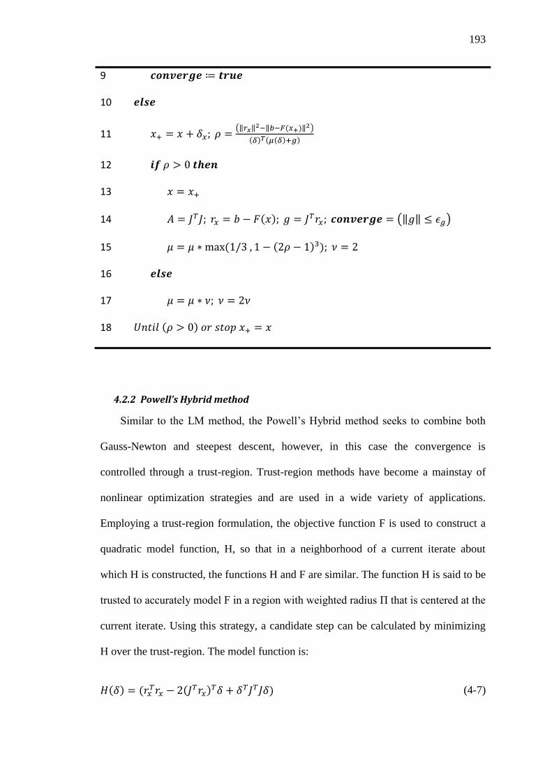
193

9 𝒄𝒐𝒏𝒗𝒆𝒓𝒈𝒆 ≔ 𝒕𝒓𝒖𝒆

10 𝒆𝒍𝒔𝒆

11 𝑥+ = 𝑥 + 𝛿𝑥; 𝜌 =(‖𝑟𝑥‖2−‖𝑏−𝐹(𝑥+)‖2)

(𝛿)𝑇(𝜇(𝛿)+𝑔)

12 𝒊𝒇 𝜌 > 0 𝒕𝒉𝒆𝒏

13 𝑥 = 𝑥+

14 𝐴 = 𝐽𝑇𝐽; 𝑟𝑥 = 𝑏 − 𝐹(𝑥); 𝑔 = 𝐽𝑇𝑟𝑥; 𝒄𝒐𝒏𝒗𝒆𝒓𝒈𝒆 = (‖𝑔‖ ≤ 𝜖𝑔)

15 𝜇 = 𝜇 ∗ max (1/3 , 1 − (2𝜌 − 1)3); 𝜈 = 2

16 𝒆𝒍𝒔𝒆

17 𝜇 = 𝜇 ∗ 𝜈; 𝜈 = 2𝜈

18 𝑈𝑛𝑡𝑖𝑙 (𝜌 > 0) 𝑜𝑟 𝑠𝑡𝑜𝑝 𝑥+ = 𝑥

4.2.2 Powell’s Hybrid method

Similar to the LM method, the Powell’s Hybrid method seeks to combine both

Gauss-Newton and steepest descent, however, in this case the convergence is

controlled through a trust-region. Trust-region methods have become a mainstay of

nonlinear optimization strategies and are used in a wide variety of applications.

Employing a trust-region formulation, the objective function F is used to construct a

quadratic model function, H, so that in a neighborhood of a current iterate about

which H is constructed, the functions H and F are similar. The function H is said to be

trusted to accurately model F in a region with weighted radius Π that is centered at the

current iterate. Using this strategy, a candidate step can be calculated by minimizing

H over the trust-region. The model function is:

𝐻(𝛿) = (𝑟𝑥𝑇𝑟𝑥 − 2(𝐽𝑇𝑟𝑥)𝑇𝛿 + 𝛿𝑇𝐽𝑇𝐽𝛿) (4-7)

194

and a candidate step can be attained by solving:

min𝛿 𝐻(𝛿) 𝑠𝑢𝑏𝑗𝑒𝑐𝑡 𝑡𝑜 ‖𝛿‖ ≤ Π. (4-8)

In practice, the trust region radius is selected based on the ability of the model to

‘fit’ the objective function - strong agreement between the approximation and the

original model suggest a strong value of Π. The solution to the trust-region in

Equation (4-1) can be seen in Figure 4-1. In his seminal paper, Powell (Powell, 1970)

used piecewise linear trajectories consisting of two line segments in order to

approximate the solution curve. In other words, rather than solving the normal

equations directly, which can be expensive, Powell approximated the solution using

two less expensive calculations. The first segment emanates from the current

approximation to the so-called Cauchy point which is the unconstrained minimum of

the objective function along the steepest descent (or gradient) plane, 𝐽𝑇𝑟𝑥 and is given

by:

𝛿𝑠𝑑 ≔𝑔𝑇𝑔

𝑔𝑇𝐽𝑇𝐽𝑔𝑔, (4-9)

the second component runs from this 𝛿𝑠𝑑 to the Gauss-Newton step. Table 4-2

summarizes the Powell’s Hybrid algorithm.

Table 4-2. Powell’s Hybrid method algorithm

Input: A function 𝐹: ℜ𝑛 → ℜ𝑛 and initial estimate 𝑥0 ∈ ℜ𝑛 and output parameters b Output: A vector 𝑥∗ ∈ ℜ𝑛 where 𝐹(𝑥∗) ≈ 𝑏 1 𝑘 ≔ 0; Π ≔ Π 0; 𝑥 ≔ 𝑥0 2 𝐴 ≔ 𝐽𝑇𝐽; 𝑟𝑥 ≔ 𝑏 − 𝐹(𝑥); 𝑔 ≔ 𝐽𝑇𝑟𝑥

3 𝒄𝒐𝒏𝒗𝒆𝒓𝒈𝒆 ≔ (‖𝑔‖ ≤ 𝜖𝑔)

4 𝒘𝒉𝒊𝒍𝒆 (𝑘 < 𝑘𝑚𝑎𝑥 𝑎𝑛𝑑 𝒄𝒐𝒏𝒗𝒆𝒓𝒈𝒆 = 𝒇𝒂𝒍𝒔𝒆) 𝒅𝒐

5 𝑘 = 𝑘 + 1

195

6 𝛿𝑠𝑑 =‖𝑔‖2

‖𝐽𝑔‖𝑔

7 𝑮𝒂𝒖𝒔𝒔 𝑵𝒆𝒘𝒕𝒐𝒏 = 𝒇𝒂𝒍𝒔𝒆

8 𝑹𝒆𝒑𝒆𝒂𝒕

9 𝒊𝒇 (‖𝛿𝑠𝑑‖ ≥ Π) 𝒕𝒉𝒆𝒏

10 𝛿𝑑 ≔Π

𝜹𝒔𝒅𝛿𝑠𝑑

11 𝒆𝒍𝒔𝒆

12 𝒊𝒇 𝒏𝒐𝒕 𝑮𝒂𝒖𝒔𝒔 𝑵𝒆𝒘𝒕𝒐𝒏 𝒕𝒉𝒆𝒏

13 𝑺𝒐𝒍𝒗𝒆 𝐴𝛿𝑔𝑛 = 𝑔

14 𝑮𝒂𝒖𝒔𝒔 𝑵𝒆𝒘𝒕𝒐𝒏 = 𝒕𝒓𝒖𝒆

15 𝒊𝒇 (‖𝛿𝑠𝑑‖ ≤ Π) 𝒕𝒉𝒆𝒏

16 𝛿𝑑 = 𝛿𝑔𝑛

17 𝒆𝒍𝒔𝒆

18 𝛿𝑑 = 𝛿𝑠𝑑 + 𝛼(𝛿𝑔𝑛 − 𝛿𝑠𝑑)

19 𝐶ℎ𝑜𝑜𝑠𝑒 𝛼 𝑠𝑜 𝑡ℎ𝑎𝑡 ‖𝛿𝑑‖ = Π

20 𝒊𝒇 (‖𝛿𝑑‖ ≤ 𝜖𝛿) 𝒕𝒉𝒆𝒏

21 𝐶𝑜𝑛𝑣𝑒𝑟𝑔𝑒 = 𝑡𝑟𝑢𝑒

22 𝒆𝒍𝒔𝒆

23 𝑥+ = 𝑥 + 𝛿𝑑; 𝜌 =(‖𝑟𝑥‖2−‖𝑏−𝐹(𝑥+)‖2)

𝐻(0)−𝐻(𝛿𝑑)

24 𝒊𝒇 (𝜌 > 0) 𝒕𝒉𝒆𝒏

25 𝑥 = 𝑥+

26 𝐴 ≔ 𝐽𝑇𝐽; 𝑟𝑥 ≔ 𝑏 − 𝐹(𝑥); 𝑔 ≔ 𝐽𝑇𝑟𝑥

27 𝐶𝑜𝑛𝑣𝑒𝑟𝑔𝑒 ≔ (‖𝑔‖ ≤ 𝜖𝑔)

28 𝑼𝒑𝒅𝒂𝒕𝒆 Π 𝒄𝒐𝒏𝒗𝒆𝒓𝒈𝒆 ≔ (Π ≤ 𝜖𝑥‖𝑥‖)

29 𝐔𝐧𝐭𝐢𝐥 ρ > 0 or 𝐜𝐨𝐧𝐯𝐞𝐫𝐠𝐞

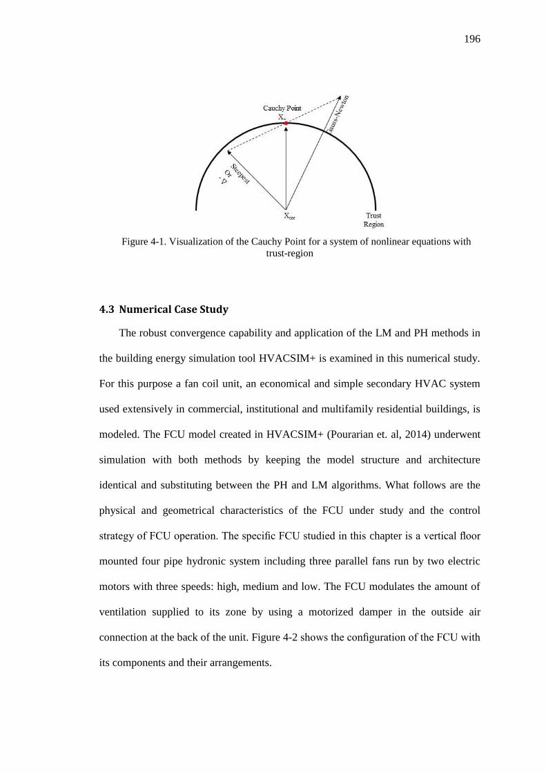
196

Figure 4-1. Visualization of the Cauchy Point for a system of nonlinear equations with

trust-region

4.3 Numerical Case Study

The robust convergence capability and application of the LM and PH methods in

the building energy simulation tool HVACSIM+ is examined in this numerical study.

For this purpose a fan coil unit, an economical and simple secondary HVAC system

used extensively in commercial, institutional and multifamily residential buildings, is

modeled. The FCU model created in HVACSIM+ (Pourarian et. al, 2014) underwent

simulation with both methods by keeping the model structure and architecture

identical and substituting between the PH and LM algorithms. What follows are the

physical and geometrical characteristics of the FCU under study and the control

strategy of FCU operation. The specific FCU studied in this chapter is a vertical floor

mounted four pipe hydronic system including three parallel fans run by two electric

motors with three speeds: high, medium and low. The FCU modulates the amount of

ventilation supplied to its zone by using a motorized damper in the outside air

connection at the back of the unit. Figure 4-2 shows the configuration of the FCU with

its components and their arrangements.

197

To simulate the FCU interacting with the corresponding zone in HVACSIM+, the

components (units) models are grouped into five blocks and each block constitutes a

superblock. The final model consists of five superblocks: control logic, actuators, air

flow, thermal, and sensors. The superblocks are weakly coupled to each other. The

solution of each superblock (obtained to some specified convergence tolerance) is the

input for the next simulation time step and this process is repeated at every time step.

The model of the FCU interacting with two exterior building zones, east and south

facing, is simulated on a summer test day. These zones are referred to as rooms in the

following discussion. In summer, the outdoor air damper is fully closed and the fan

speed is normally set at high. When the FCU is operating properly, the controller

compares room temperature to the cooling set-point (74F (23.33C)) and heating set-

point (70F (21.11 C)). If the actual room temperature is greater than (cooling set-point

−1F (0.56 C)), the FCU is in cooling mode and if it is less than (heating set-point +1F

(0.56 C)), the FCU is in heating mode. A dedicated proportional integral derivative

(PID) loop is enabled for each mode to control the cooling or heating valve position.

A PID loop is a means of regulating a process quantity (room temperature) by

compensating it with closed-loop feedback of its error (difference between the room

temperature and set-point), with the compensation amount computed linearly using

three gain coefficients.

As long as room temperature lies between the heating and cooling set-points, the

PID loops are disabled and the corresponding valves are fully closed. The room air

temperature signal is passed from the sensors superblock to the controls superblock,

which calculates the required position of the heating and cooling coil valves. Valve

positions as determined in the control superblock are passed to other superblocks as

appropriate. Simultaneous solution of mass-pressure equations occurs in the air flow

198

superblock, while energy balance equations are solved simultaneously in the thermal

superblock. As shown in Table 4-3, the total number of variables in the FCU

simulation is 58. In this table the category and number of variables in those categories

are listed. The Iowa Energy Center Energy Resource Station (ERS) provides weather

condition and experimental data necessary for simulation and validation of the FCU

model. Additional details of this model, including a discussion of model validation,

can be found in (Pourarian et. al, 2014).

Figure 4-2. Fan coil unit configuration

Table 4-3. Category and number of state variables

Category Pressure Flow

rate Temperature Control

Other (Fan

rotational speed) Power Humidity

Number of state

variables 7 8 16 14 1 8 4

In this section the simulation results of the FCU model as simulated with both

methods are presented and compared. The FCU performance variables as well as the

solver function variables are shown in order to compare the performance of the two

methods. Room air temperature and cooling coil valve position are the FCU

199

performance variables. The number of function evaluations, number of iterations,

cumulative number of iterations, and cumulative number of function evaluations are

the performance variables of each solver method.

In Figure 4-3 and Figure 4-4 the FCU performance variables of simulations for

east and south facing rooms using both the PH and LM methods are compared for

identical initial conditions. The solid line represents experimental data, the dotted line

represents the simulation result with the PH method and dashed line represents

simulation results with the LM method. The FCU model parameters have been

validated using experimental data which are reported in another publication

(Pourarian et. al, 2014). Here, experimental data serve as a reference to compare the

two solver methods.

As Figure 4-3 illustrates, the FCU in the east room is operated in cooling mode to

maintain the cooling temperature set point. The cooling coil valve controls the water

flow rate, which in part determines the heat transfer rate, and maintains the room

temperature near the cooling set point. As the east room air temperature graph in

Figure 4-3 shows, the results of the simulation for the PH and LM methods for room

air temperature are identical except for the 10:00 to 11:10 and 13:30 to 15:40 time

frames, in which the model using the PH method moves around the cooling

temperature set point but is not able to capture it. When a nonlinear system does not

converge at a given time step (i.e. the simulation fails to meet the termination

criteria), the inaccurate solution is passed to later time steps. This can lead the

simulation into non-physical state space (e.g., negative humidity) and/or an inaccurate

solution. This can happen when residuals become small, but fail to vanish. Thus,

while all but one superblock may reach convergence within a time step, the one

superblock that failed to converge can cause the entire simulation to fail at that time

200

step. That scenario is avoided by the LM method, which successfully iterates all

superblocks to desirable solutions within the simulation time window. For this reason,

the simulation result for cooling coil valve position by the LM method is reasonable,

whereas the solution provided by the PH method is not. The bump that occurs around

11:00 in the east room air temperature values calculated by the PH method shows that

solver became trapped in an unsatisfactory region where it could not find the

minimum of the sum of the squares of the functions.

Figure 4-3. Simulation results of FCU operational variables in east room by PH and LM

method

As Figure 4-4 shows, the FCU operation in the south room is consistent with the

operation in the east room. The PH method did not solve the thermal superblock in the

10:00 to 11:10 and 13:10 to 15:45 time frames, having completed all iterations

unsuccessfully. On the other hand, the LM method converged to a desirable solution

for both the air flow and thermal superblocks. The simulation results predicting the

FCU operation in the east and south rooms are acceptable when the solver returns a

converged solution for all superblocks. As the south room air temperature graph in

Figure 4-4 shows, the results of the simulation for the PH and LM methods for room

air temperature are identical except for the 10:00 to 11:10, 13:10 to 14:00 and 14:30

201

to 16:00 time frames, in which the PH method moves around the cooling temperature

set point but is not able to capture it. The cooling coil valve position based on the LM

method, which successfully converged to a solution, gives more reasonable results.

The prior validation work (Pourarian et. al, 2014) revealed some weaknesses in

the combined model of the FCU and room. The thermodynamic interaction between

the modeled room and the ambient environment differs from the interaction that

occurs in the real physical space. Thus, the cooling coil valve signals solved for in the

control superblock do not completely agree with the experimental data. This weakness

in the model is most clearly demonstrated by the decrease in cooling coil valve

position shown near 14:00 in Figure 4-4 for both the PH and LM methods.

Figure 4-4. Simulation results of FCU operational variables in south room by PH and LM

method

Figure 4-5- Figure 4-8 are a brief comparison of the PH and LM method

performance variables obtained in solving the system of nonlinear equations that

emerge in the FCU simulation. Figure 4-5 is a comparison of the PH and LM method

cumulative number of iterations and the number of iterations at each time step in the

air flow and thermal superblocks for the FCU in the east room. Similarly, Figure 4-6

displays the comparison of the PH and LM method cumulative number of function

202

evaluations and the number of function evaluations at each time step in the air flow

and thermal superblocks for the FCU in the east room; Figure 4-7 and Figure 4-8

display the same data for the south room. According to the number of iterations at

each time step for the thermal superblock of the FCU in the east and south room in

Figure 4-5 and Figure 4-7, it is obvious that for the PH method, during the time

frames with unsuccessful solutions, the number of iterations in the thermal superblock

is greater. This implies that the PH method attempts to make good progress toward

the solution by increasing the number of iterations. A close look at the number of

function evaluations in Figure 4-6 and Figure 4-8 for the FCU thermal superblock in

the east and south rooms leads us to the same conclusion. Note that in Figure 4-8, near

14:00 the number of function evaluations does not spike for either PH or LM because,

as noted above, the deviation from the experimental data is not due to convergence

failure.

Figure 4-6 and Figure 4-8show that the LM method requires more function

evaluations than the PH method because, as discussed in Section 4.2, the LM method

solves the normal equations directly rather than using the approximation employed in

the PH method. Figure 4-5 and Figure 4-7 show that, for the airflow superblock, the

LM method requires more iterations than the PH method; this is also a result of the

direct solution of the normal equations. In Figure 4-7, for the thermal superblock, the

LM method requires more iterations than the PH method, as expected, but in Figure

4-5, the thermal superblock requires more iteration for the PH method than for the

LM method. This behavior demonstrates the difficulty that the PH method has

converging to a solution in the thermal superblock for the east room as previously

discussed in relation to Figure 4-3. If both methods are properly converging, the LM

method should require more iterations than PH due to its greater complexity.

203

Figure 4-5. Comparison of the cumulative number of iterations and the number of

iterations at each time step for the PH and LM methods in the air flow and thermal

superblocks for the FCU in the east room. In the air flow superblock the LM method rapidly

oscillates between seven and eight iterations, resulting in what appears to be a solid block.

Figure 4-6. Comparison of the cumulative number of function evaluations and the number

of function evaluations at each time step for the PH and LM methods in the air flow and

thermal superblocks for the FCU in the east room. In the air flow superblock the LM method

rapidly oscillates between seven and eight iterations, resulting in what appears to be a solid

block.

204

Figure 4-7. Comparison of the cumulative number of iterations and the number of

iterations at each time step for the PH and LM methods in the air flow and thermal

superblocks for the FCU in the south room. In the air flow superblock the LM method rapidly

oscillates between seven and eight iterations, resulting in what appears to be a solid block.

Figure 4-8. Comparison of the cumulative number of function evaluations and the number

of function evaluations at each time step for the PH and LM methods in the air flow and

thermal superblocks for the FCU in the south room. In the air flow superblock the LM method

rapidly oscillates between seven and eight iterations, resulting in what appears to be a solid

block.

205

4.4 Conclusion and summary

A qualitative difference between the LM and PH methods arises when a trial step

fails to yield sufficient decrease in the residual of the nonlinear equations and the

search direction must be altered. Many simple methods for solving nonlinear

equations simply shorten the length of the search trial step in hopes that a shorter step

will yield sufficient decrease of the residuals. Other more sophisticated techniques

alter both the length and the direction of the trial step. In the case of LM, the µ

parameter is increased and the resulting Eq. (4-6) is solved. This is the case even

when a trial step with length less than that of the Cauchy step yields sufficient

decrease in the residuals of the nonlinear equations and this trial step is an acceptable

step. On the other hand, when PH computes a trial step, it is generated by augmenting

or ‘adding onto’ the Gauss-Newton step. Once the Gauss-Newton step has been

computed at a given point, the PH algorithm computes trial steps by changing the

parameter Π. The PH algorithm, therefore, computes all trial steps, both successful

steps and failed steps, without resolving the normal equations, (Eq. (4-7)). This is true

even when a trial step with length less than the length of the Cauchy step is chosen to

be the accepted step of PH. Where the LM method solves the normal equations, the

PH method uses an approximation. This is the reason for the improvements in the LM

method over the PH method, but it is also the reason why the LM method can be more

computationally expensive.

An important computational issue that arises in the multiphysics framework of

modelling buildings is that of preconditioning of nonlinear systems. This occurs when

two or more component models are coupled with the goal of simulating events

involving the output from these components. Many linear preconditoners exist for

applications-specific linear systems; however, in the context of improving

206

HVACSIM+, greater improvement can be seen from considering directly the

nonlinear system coupling components. Future research will focus on improving the

problem formulation by developing and applying a preconditioner that is designed

specifically for HVAC applications. This process will include creating a more

uniform scaling across variables and ordering the solution of equations in a way that

is numerically stable.

207

5. CHAPTER FIVE: MODIFICATION AND VALIDATION OF BUILDING ZONE MODEL

5.1 Introduction

The application of lumped parameter modelling methods to building dynamic

thermal response is motivated by the desire to find simpler and, hence,

computationally less expensive methods for the analysis building thermal energy

response. Furthermore, this method simplicity and competence for full simulations

including control system analysis and AFDD methods have been highlighted in the

literature. Approaches broadly fall into two categories:

• Lumped parameter construction element models from which whole room

models may be constructed (Gouda et al., 2002; Lorenz et al., 1982; Fraisse et al.,

2002, Chaturvedi et al., 2002)

• Lumped parameter whole room models (Crabb et al., 1987; Tindale, 1993;

Nielsen, 2005; Kampf et al., 2007; Antonopoulos et al., 2001)

Though the differences between the two approaches are rather subtle (since

models of individual construction elements are almost always used as a basis for

grouping or aggregating into whole room models), the treatment of individual

elements usually provide greater detail in modelling information such as individual

surface temperatures which can be important when dealing with radiant sources, etc.

Lorenz et al., 1982, were among the first to propose a simplified lumped

parameter approach to building response modelling using a first-order model

consisting of two resistances and one capacitor. Gouda et al., 2002, demonstrated

improved accuracy using a second order model in which each construction element is

described using three resistances and two capacitances. These approaches to

modelling were often referred to as ‘analogue circuit’ models due to their similarity

with electric circuits.

208

Fraisse et al., 2002, also compared first- and second-order element models (the

latter referred to as a ‘3R2C’ model) and went further to propose a fourth-order

‘3R4C’ model with aggregated resistances. Like Lorenz et al. they propose an

analytical method for deriving the parameters of the model (essentially, the

distribution of resistance and capacitance values throughout the ‘circuit’) whereas

Gouda et al. and Chaturvedi et al. used an optimization method to determine the

parameters with reference to a rigorous reference model.

Crabb et al., Tindale, Nielsen et al. Kampf et al. and Antonopoulos et al. have

applied the lumped parameter approach to the formulation of low-order whole room

models by casting the capacitance parameter over the higher capacity elements of a

room (external walls, solid floors, etc.) and using algebraic heat balances for the lower

capacity room elements (demountable partitions, etc.). Tindale attempted this using a

second-order room model but found that it provided unacceptable results for rooms

with very high thermal capacity (i.e. ‘traditional’ construction). He corrected this by

introducing a third ‘equivalent’ room capacitance which required an inconvenient

method for its parameterization.

Though low-order whole room models offer very low computational demands

and simplicity, there remain questions over the accuracy of these models particularly

over long time horizons and they tend to provide less modelling information (i.e.

individual and accurate element surface temperatures) essential in many lines of

design enquiry. For this reason, it is argued that room models constructed from

second-order (or higher) construction element descriptions provide greater accuracy

and detail whilst retaining some of the key advantages of simplicity and low

computational demand and are, therefore, to be preferred other than for approximate

and early feasibility simulation studies. The key advantage of using lumped parameter

209

method to represent buildings is that they can be mathematically modelled by a set of

first order differential equations; also called state-space systems. The integration of

these systems provides the variables of the model (temperatures of building elements

and zones) at a relatively low computational cost. The short computational times

made these models popular during the 1970s when computational resources were

limited. However they are still used when quick building simulators are needed to

perform a large number of simulations (Coley et al., 2002; Kampf et al., 2009 and

Kershaw et al., 2011). They are particularly suited to research-based building

response modelling using either modular-graphical modelling tools or equation based

methods and also to applications involving detailed systems, plant and control

simulations requiring accurate short-term building model performance at minimum

computer time.

5.2 Building Zone Thermal Model in HVACSIM+ Library of Component

Building zones characterized by a uniform temperature and a perfectly mixed

volume (supposed to be thermally homogeneous) are modeled by TYPE 403 in

HVACSIM+ library of components. In TYPE 403, each building zone is composed of

two sets of Two-Capacitor–Three-Resistor (2C3R) LMP model (Norford and Haves,

1997, DeSimone, 1996). One set of 2C3R model represents the occupied space and

the contents of the zone and the other set represents the corresponding plenum or

unoccupied space and its contents (Figure 5-1). The two sets of 2C3R models are

coupled together with a connecting resistance (R11) which represents the ceiling

separating the two spaces. As Figure 5-1 illustrates for each building zone, there are

eleven parameters which need to be determined.

In Figure 5-1 the upper 2C3R network is representative of plenum and the lower

one is room model the connecting resistance of the two networks (R11) is

210

representative of ceiling. The constitutive resistances and capacitances of plenum

2C3R network are:


proportioned structural resistances. C22 and C23 are internal and structural capacitance

respectively.

Zone 2C3R network is composed of:


proportioned structural resistances. C02 and C03 are internal and structural capacitance

respectively.

Heat sources for zone directly added to the internal air node of zone network are

lighting and equipment (Qr) and occupant (Qo) and HVAC heat gain (Qv). Similarly

heat gain in the plenum (Qp) is added to the internal air node of the plenum network.

Tpa and Tra are temperatures of the internal air and all light structures in the

plenum and room model which are calculated in TYPE 403 as a weighted average,

taking into account the influences of surrounding walls, the outside ambient air,

leakage and infiltration from adjacent zones, and the supply air (Norford and Haves,

1997, DeSimone, 1996). Tp and Tr are plenum and zone structure temperature and Tsa

is sol-air temperature.

Figure 5-1. Illustration of a 2C3R model for a building zone (DeSimone,1996)

211

To determine the global parameters of 2C3R network, the resistances and

capacitances of all individually identifiable walls, floor and ceiling components of the

zone including internal, external and connecting walls are needed to be defined. The

global model is an attempt to bring together a large number of individual systems in

order to render a complex system into a simple network replicating the real behavior

of the building zones. The details about the procedure and equations used to

determine the resistance and capacitance of different constitutive components of the

zone which consequently lead to determine the parameters for 2C3R global model are

provided by DeSimone (1996) and are summarized here.

The individual walls are represented by two resistors and one capacitor. The

thermal capacitance is located between the two thermal resistors at a location in the

wall specified by a weighting factor m. The walls are assumed to be comprised of

“N” definable layers, each characterized by a resistive element and a capacitive

element. Air boundary layers on both sides of the walls are accounted for as

individual resistive elements, adding two additional resistors to the “N” wall layers

combines for a total of “N+2” series resistors in each wall section. The “N+2”

resistive elements are summed in series to obtain an overall resistance (Eq.(5-1)). The

“N” capacitances are summed to obtain an overall capacitance (Eq.(5-2)), and the

weighting factor is calculated by (Eq. (5-3)).

𝑅𝑚 = ∑ 𝑅𝑚,𝑛

𝑁+1

𝑛=0

(5-1)

𝐶𝑚 = ∑ 𝐶𝑚,𝑛

𝑁

𝑛=1

(5-2)

𝜃𝑚 = 1 − ∑(∑ 𝑅𝑚,𝑝 +

𝑅𝑚,𝑛

2𝑛−1𝑝=0 ) 𝐶𝑚,𝑛

𝑅𝑚𝐶𝑚

𝑁

𝑛=1

(5-3)

212

A time constant, expressed as a function of Rm, Cm and m. in Eq. (5-4) is used to

differentiate between light and heavy walls and sub-walls or structures.

𝜏𝑚 = 𝜃𝑚(1 − 𝜃𝑚)𝑅𝑚𝐶𝑚 (5-4)

Where: m≤limit→light structure;

m＞limit→Heavy structure; and

the approximate limits for limit are 1 hour ≤limit ≤ 2 hour.

Each of the resistive elements within the 2C3R zone model is defined as follows:

𝑅01 =1

𝐾𝑙𝑖𝑡𝑒,𝑒𝑥𝑡 (5-5)

𝑅02 =1

𝐾ℎ𝑣𝑦,𝑖𝑛𝑛𝑒𝑟𝜃𝑖 (5-6)

𝑅03 =1

𝐾ℎ𝑣𝑦,𝑖𝑛𝑛𝑒𝑟(1 − 𝜃𝑖) (5-7)

where 𝐾𝑙𝑖𝑡𝑒,𝑒𝑥𝑡 is the conductance of internal structure directly to outside through

light walls and 𝐾ℎ𝑣𝑦,𝑖𝑛𝑛𝑒𝑟 is the conductance of inner portion of heavy walls. The

factor 𝜃𝑖 (global accessibility of structural capacitance) is expressed by,

𝜃𝑖 =𝐾ℎ𝑣𝑦,𝑒𝑥𝑡

𝐾ℎ𝑣𝑦,𝑖𝑛𝑛𝑒𝑟 (5-8)

where 𝐾ℎ𝑣𝑦,𝑒𝑥𝑡 is the conductance of heavy external wall. The conductance

variables, Klite, ext, Khvy, inner, and Khyy,ext expressed in terms of composite

resistance values are defined as follows:

𝐾𝑙𝑖𝑡,𝑒𝑥𝑡 = ∑(1 − 𝐻𝑚)𝐸𝑚

𝑅𝑚𝑚

(5-9)

𝐾ℎ𝑣𝑦,𝑖𝑛𝑛𝑒𝑟 = ∑𝐻𝑚

𝑅𝑚𝜃𝑚𝑚

(5-10)

𝐾ℎ𝑣𝑦,𝑒𝑥𝑡 = 𝐾𝑒𝑥𝑡 − 𝐾𝑙𝑖𝑡,𝑒𝑥𝑡; or (5-11)

213

𝐾ℎ𝑣𝑦,𝑒𝑥𝑡 = ∑𝐸𝑚

𝑅𝑚𝑚

− ∑(1 − 𝐻𝑚)𝐸𝑚

𝑅𝑚𝑚

Where: Em= 0 for each internal wall or connection sub-wall

Em= 1 for each external wall

Hm= 0 for all wall or sub-walls with τm ≤ τlimit (light walls)

Hm= 1 for all wall or sub-walls with τm ＞ τlimit (heavy walls)

The time constant τi which characterizes the response to excitation for the zone

system ascribed to each zone is expressed in the following equation:

𝜏𝑖 =1

𝐾𝑖∑(1 − 𝜃𝑚𝐸𝑚)𝐻𝑚𝐶𝑚

𝑚

(5-12)

The conductance Ki is defined as the overall loss coefficient and is expressed in

terms of Ci,out (the capacitive flow of infiltration in zone i based on the volumetric

flow rate Vi,out for infiltration) and Kext (the overall loss coefficient for the heavy

walls) in the following equations:

𝐾𝑖 = 𝐶𝑖,𝑜𝑢𝑡 + 𝐾𝑒𝑥𝑡 ; where (5-13)

𝐶𝑖,𝑜𝑢𝑡 = 𝜌𝑎𝐶𝑝𝑎𝑉𝑖,𝑜𝑢𝑡 ; and (5-14)

𝐾𝑒𝑥𝑡 = ∑𝐸𝑚

𝑅𝑚𝑚

(5-15)

The infiltration volumetric flow rate Vi,out is calculated by 0.37 CFM per feet of

exterior window’s sash crack (Pita, 2002).

The structural capacitance parameter C03,i represents the heavy structures in the

zone model. It is expressed in terms of the overall heavy structure capacitance and a

factor which characterizes the response of the 2C3R network to step changes in

internal heat flux and outdoor temperature.

214

𝐶03 = 𝐾𝑖𝜏𝑖

(1 −𝜉𝑖𝐾𝑖

𝐾𝑒𝑞,𝑖)

2

(1 −𝐾𝑖

𝐾𝑒𝑞,𝑖)

(5-16)

The conductance Keq,i is described as the equivalent resistance for zone i and is

expressed in the following equation:

𝐾𝑒𝑞,𝑖 = 𝐶𝑖,𝑜𝑢𝑡 + 𝐾𝑙𝑖𝑡,𝑒𝑥𝑡 + 𝐾ℎ𝑣𝑦,𝑖𝑛𝑛𝑒𝑟 (5-17)

and the term 𝜉𝑖 is described as the ratio of heat loss through the light walls to the

total heat loss to the outside:

𝜉𝑖 =𝐶𝑖,𝑜𝑢𝑡 + 𝐾𝑙𝑖𝑡,𝑒𝑥𝑡

𝐶𝑖,𝑜𝑢𝑡 + 𝐾𝑒𝑥𝑡 (5-18)

The internal capacitance parameter C02,i represents the light structures and the air

contained within the zone. It is simply the sum of the represented thermal capacitance

values:

𝐶02 = 𝐶𝑎,𝑖 + ∑ 𝐶𝑚(1 − 𝜃𝑚𝐸𝑚)(1 − 𝐻𝑚)

𝑚

(5-19)

The term Ca,i represents the capacitance for the air within zone I

(𝜌𝑟𝑜𝑜𝑚 𝑎𝑖𝑟𝐶𝑝,𝑟𝑜𝑜𝑚 𝑎𝑖𝑟𝑉𝑟𝑜𝑜𝑚 𝑎𝑖𝑟. The sum adds the entire contribution from the light,

internal walls to a fractional contribution from the light, external walls.

In summary, for each building zone, there are eleven parameters (R01, R02, R03,

C02, C03, R11, R21, R22, R23, C22, C23) which need to be determined. To determine

these eleven parameters, there are even more intermediate parameters that need to be

calculated.

215

5.3 Solar Gains and Sky Radiation

Solar gains and sky radiation are expressed through the definition of an

equivalent “sol-air” temperature tsa,i. The overall, equivalent temperature represents an

estimate of the energy flux across the external zone barriers. It is weighted average

taking into account the effect of all incident radiation on all surfaces for each

individual zone. Normally, weighting is derived from ratios of the conductance for the

surfaces of similar optical characteristics and physical orientation within a given zone

to the conductance for the entire external zone surface. The overall, equivalent sol-air

temperature incorporating the effect of opaque surfaces, single pane windows and

general barriers of any configuration is expressed in the following equation:

𝑇𝑠𝑎,𝑖 =∑ 𝐾𝑒𝑥𝑡,𝑚 𝑡𝑠𝑎,𝑚,𝑖,𝑜𝑝𝑎𝑞𝑚

𝐾𝑖+

∑ 𝐾𝑒𝑥𝑡,𝑚 𝑡𝑠𝑎,𝑚,𝑖,𝑠𝑖𝑛𝑔𝑚

𝐾𝑖 (5-20)

The conductance Ki and Kext,m are previously defined and the sol-air temperatures

for the various barrier types are expressed as follows:

𝑡𝑠𝑎,𝑚,𝑖,𝑜𝑝𝑎𝑞 = 𝑡𝑜𝑢𝑡 +1

ℎ𝑜𝑢𝑡,𝑚,𝑖(𝛼𝑚,𝑖𝐼𝑔,𝑚,𝑖 − 𝜖𝑚,𝑖𝐼𝑟,𝑚,𝑖) (5-21)

𝑡𝑠𝑎,𝑚,𝑖,𝑠𝑖𝑛𝑔 = 𝑡𝑜𝑢𝑡 +1

ℎ𝑜𝑢𝑡,𝑚,𝑖(𝛼𝑚,𝑖𝐼𝑔,𝑚,𝑖 − 𝜖𝑚,𝑖𝐼𝑟,𝑚,𝑖) +

𝜏𝑚,𝑖𝐼𝑔,𝑚,𝑖

𝑈𝑚,𝑖 (5-22)

Where: 𝑡𝑠𝑎,𝑚,𝑜𝑝𝑎𝑞= the sol-air temperature for an opaque wall

𝑡𝑠𝑎,𝑚,𝑠𝑖𝑛𝑔 = the sol-air temperature for a single pane window

The coefficients included in Eqs. (5-21) and (5-22) are defined as follows:

𝐼𝑟,𝑚,𝑖= the longwave heat transfer between the outer surface of wall m in zone i

and the sky cover (W/m2)

𝐼𝑔,𝑚,𝑖= the shortwave solar gain on the outer surface of wall m in zone i (W/m2)

216

𝑈𝑚,𝑖= the overall conductive heat transfer coefficient for wall m in zone i (W/◦K

m2)

𝛼𝑚,𝑖= the outer surface absorptance of wall m in zone i

휀𝑚,𝑖= the emissivity of the outer surface of wall m in zone i

𝜏𝑚,𝑖= the transmittance of the outer surface of wall m in zone i

ℎ𝑜𝑢𝑡,𝑚,𝑖= film coefficient for exterior surface of wall m in zone I (W/◦K m

2)

𝑡𝑜𝑢𝑡= outdoor air dry bulb temperature (◦C)

5.3.1 Calculating the long-wave heat transfer

The heat flux 𝐼𝑟,𝑚,𝑖 across surface m can be expressed as a function of the long-

wave (infrared) sky radiative transfer of a horizontal surface to the celestial surface

and the angle sm of surface m (measured from horizontal):

𝐼𝑟,𝑚,𝑖 =1 + cos 𝑠𝑚

2𝐼𝑟,ℎ 𝑆𝑚 < 90 (5-23)

Where 𝐼𝑟,ℎ is defined as the long-wave sky radiative transfer of a horizontal

surface. Typical values for 𝐼𝑟,ℎ range between 100 W/m2 for clear sky condition to 45

W/m2 for overcast conditions. When figuring what value to use, cloud cover data can

provide a basis for factorization the difference between the two extremes. For

𝑠𝑚 = 90 the value 0.5 𝐼𝑟,ℎ is used.

5.3.2 Calculating the short-wave heat transfer

The total solar gain 𝐼𝑔,𝑚,𝑖 on the external surface of wall m is the sum of the

direct solar radiation 𝐸𝐷, the total diffuse radiation 𝐸𝑑 from the sky and ground and

the solar radiation reflected from the surroundings 𝐸𝑟 as follows:

𝐼𝑔,𝑚,𝑖 = 𝐸𝐷 + 𝐸𝑑 + 𝐸𝑟 (5-24)

where:

217

𝐸𝐷 = 𝐸𝐷𝑁 cos 𝜃𝑣 (5-25)

And

𝐸𝑑 = 𝐸𝑑𝑠 + 𝐸𝑑𝑔 (5-26)

With 𝐸𝐷𝑁 = the direct normal irradiance;

𝜃𝑣 = the incident angle of the sun to the surface of wall m;

𝐸𝑑 = total diffuse radiation from the sky and ground;

𝐸𝑑𝑠 = diffuse radiation from the sky;

𝐸𝑑𝑔 = diffuse radiation from the ground;

5.3.3 Calculating the reflected solar radiation Er

Er is considered to be negligible for ERS building. Because, the building is open

with an unobstructed view to all orientations.

5.3.4 Calculating the direct normal irradiance EDN

For this project, direct normal irradiance is provided by the test facility and 𝜃𝑣

can be calculated following the procedure outlined in the next section.

5.3.5 Calculating the total diffuse radiation from sky and ground Ed

Here ASHREA handbook method is used to determine total diffuse radiation.

Based on this method the diffuse sky radiation Eds for vertical and horizontal surfaces

can be expressed in terms of EDN. some trigonometric relations relates to the

orientation of the surface receiving the radiation, and a factor representing the degree

of scatter introduced by the atmosphere as a function of the earth’s relative position to

the sun:

𝐸𝑑𝑠,𝑣𝑒𝑟𝑡 = 𝐶 𝑌 𝐸𝐷𝑁 ; and (5-27)

𝐸𝑑𝑠,𝜎≠90 = 𝐶 𝐸𝐷𝑁(1+cos 𝜎)

2 ; where (5-28)

218

𝑌 = 0.55 + 0.437 cos 𝜃 + 0.313 cos2 𝜃 ∀ cos 𝜃 > −0.2; (5-29)

Otherwise Y=0.45 (5-30)

And: C = Sky diffuse factor

The sky diffuse factor is a dimensionless ratio indicating the effect of the earth’s

relative position to the sun throughout the year, proportioning the effect of the direct

normal irradiance as the season change. Values for C over the course of a year have

been provided in ASHRAE fundamentals. It should be noted that this coefficient is

affected by the local levels of smog, water vapor, and suspended dust in the

atmosphere.

The diffuse radiation reflected from the ground is expressed as a function of the

direct normal radiation:

𝐸𝑑𝑔 =𝐸𝐷𝑁(𝐶 + sin 𝛽)𝜌𝑔(1 − cos 𝜎)

2 (5-31)

Where: C = Sky diffuse factor;

𝛽 = Solar altitude;

𝜌𝑔 = Ground reflectance; and

𝜎 = receiving surface tilt angle from horizontal.

The coefficient C in this expression intensifies the effect of the direct normal

irradiance as the season change. Again this effect is, in practice, subject to local

variations in atmosphere conditions. The solar altitude 𝛽 is calculated in Eq. (5-36).

The ground reflectance is assumed to be 0.2. For this research, 𝜎 is equal to either 90

for vertical or 0 for horizontal surfaces.

219

5.3.6 Incident angle 𝜽 and solar altitude 𝜷

The incident angle 𝜃𝑣 can be expressed, in general for any surface orientation, as

a function of the solar altitude β, the surface solar azimuth 𝛾, and surface tilt angle 𝜎

as follows:

cos 𝜃 = cos 𝛽 cos 𝛾 sin 𝜎 + sin 𝛽 cos 𝜎 (5-32)

For vertical surfaces (𝜎 = 90) and with 𝛾 expressed in terms of the solar azimuth

ϕ and the surface azimuth ψ Eq. (5-32) becomes:

cos 𝜃𝑣 = cos 𝛽 cos(𝜙 − 𝜓) (5-33)

For horizontal surfaces (𝜎 = 90) and with 𝛾 expressed in terms of ϕ and ψ Eq.

(5-32) becomes:

cos 𝜃ℎ = sin 𝛽 (5-34)

The surface azimuth ψ is obtained from ASHRAE fundamentals, and the solar

azimuth angle ϕ (a function of the solar altitude β, local latitude L, and the solar

declination δ) can be calculated:

cos 𝜙 = sin 𝛽 sin 𝐿 − sin 𝛿

cos 𝛽 cos 𝐿 (5-35)

The solar altitude β is a function of local latitude L, solar declination δ and

apparent solar time expressed as an hour angle H:

sin 𝛽 = cos 𝐿 cos 𝛿 cos 𝐻 + sin 𝐿 sin 𝛿 (5-36)

𝐻 = 0.25 × 𝑀𝑛𝑢𝑚𝑏𝑒𝑟 𝑜𝑓 𝑚𝑖𝑛𝑢𝑡𝑒𝑠 𝑓𝑟𝑜𝑚 𝑙𝑜𝑐𝑎𝑙 𝑠𝑜𝑙𝑎𝑟 𝑛𝑜𝑜𝑛 (5-37)

𝑀𝑛𝑢𝑚𝑏𝑒𝑟 𝑜𝑓 𝑚𝑖𝑛𝑢𝑡𝑒𝑠 𝑓𝑟𝑜𝑚 𝑙𝑜𝑐𝑎𝑙 𝑠𝑜𝑙𝑎𝑟 𝑛𝑜𝑜𝑛

= 720 − 𝐴𝑆𝑇𝑖𝑛 𝑚𝑖𝑛𝑢𝑡𝑒𝑠 𝑎𝑓𝑡𝑒𝑟 𝑚𝑖𝑑𝑛𝑖𝑔ℎ𝑡 (5-38)

220

𝐴𝑆𝑇 = 𝐿𝑆𝑇 + 𝐸𝑇 + 4(𝐿𝑆𝑀 − 𝐿𝑂𝑁) (5-39)

Where: LST = local standard time (minutes);

ET = the equation of time (minutes of time);

LSM= local standard time meridian (degrees of arc);

LON= local longitude (degree of arc);

4 = minutes of time required for 1.0 degree rotation of earth

5.4 The Issues Associated with the Zone Model in HVACSIM+ Library of

Component

In order to investigate the zone model in HVACSIM+ library of component,

TYPE 403 needs to undergo a close study as an isolated unit. For this reason, The

inputs to the model which include supply air dry bulb temperature, humidity ratio and

mass flow rate, ambient dry bulb temperature and humidity ratio, room and plenum

sol-air temperatures as well as internal heat gain (occupant, light and equipment) need

to be provided to the model from experimental data. The only output of the model

which can be compared against experimental data is the room temperature which is

also recorded at the test facility. A comprehensive study has been done to investigate

the issues associated with the existing 2C3R model in HVACSIM+ component

library. The outcome of this study is applied toward 2C3R zone model improvement.

5.4.1 Assumptions for zone model study

Originally in TYPE 403, all resistances and capacitances are assumed to be time

invariant. Thus, the effect of varying wind velocity on external convection

coefficients and room pressurization is not considered. Furthermore, TYPE 403

characterizes building zones by a uniform temperature and a perfectly mixed volume.

In order to study the zone model as an independent unit some assumption has been

made as following:

221

• No air leakage from/to outside

• No flow from/to adjacent zone 1 & 2

• No heat gain/loss from supply duct

• No heat gain/loss from return duct

5.4.2 Zone model comprehensive study

At the preliminary study the experimental data provided by ERS for fan coil unit

in east, south and west facing rooms on a normal summer test day were picked to be

fed to the model as inputs. Figure 5-2 illustrates the comparison of east, south and

west facing rooms simulation result with experimental data on a summer test day

(07.15.2012). The first graph at the top shows the ambient temperature and supply air

temperature provided by FCU to each room. As this Figure demonstrates, there is a

large deviation of the model results from experimental data for all rooms. While the

provided supply air conditions and flow rate (0.421 kg/s (745 CFM)) to the rooms are

the same as experiment, the modeled room is unable to keep room air temperature set

point. Since fan coil unit is functioning in cooling mode, the room temperature is to

be maintained at cooling set point temperature. In the legend of all following figures

including this section and the next ones, CLGSTP and HTGSTP refer to cooling set-

point and heating set-point respectively.

Figure 5-2 demonstrates that under the defined conditions based on the

experimental data the simulated rooms get overcooled. The simulated room air

temperature is representative of well mixed air within the room, but in reality the

room temperature sensor may reflect a local temperature that is not necessarily

reflective of a bulk room temperature. Furthermore, simulated zone is more sensitive

to changes in internal load and fluctuations in supply air flow rate and temperature

than the actual zone. As Figure 5-2 shows the simulated room temperature has

222

particularly sharp spikes in the absence and presence of equipment heat load at

minutes 480 (presence), 720 (absence), 780 (presence) and 1020 (absence) (refer to

Figure 5-3). The dynamics of the modeled zone display some deviation from the real

one due in part to unavoidable simplification which needs to be thoroughly addressed.

223

Figure 5-2. Comparison of simulation result with FCU experimental data for isolated zone

model

224

Figure 5-3. Fractional internal loads including occupant, lighting and equipment heating

load as time dependent boundary conditions

Based on the comparison of the modeled zone results with real room temperature,

a close observation in the following direction is needed:

1) Solar radiation through glazing: the existing 2C3R model does not consider

the radiation received by the rooms through transparent surfaces

2) Optimizing the zone model physical parameters: as Figure 5-2 shows, the

discrepancy of the zone model and experimental data at the beginning and

late hours of the day cannot be related to the lack of the model in simulating

the transmitted radiation. The main reason resides in the physical parameters

of the zone model. It is partly due to the assumptions associated with the

simulation and also the simplifications involved with the model to make it

computationally efficient and feasible.

3) The uncertainty associated with the measured data: The uncertainty

associated with sensors in collecting experimental data is unavoidable. As far

as using experimental data as input to the model, this uncertainty propagates

to the simulation as well as validation. For example, in the preliminary study

the ERS experimental data collected for FCU has been used. The FCU supply

225

air temperature is recorded at one point. Obviously, in order to have a semi

accurate supply air temperature the average of various point measurements at

the outlet of FCU is needed.

5.4.2.1 Transmitted solar radiation through glazing

In the proposed 2C3R model for zone in TYPE 403 of HVACSIM+ the internal

heat sources are confined to occupant, lighting and equipment heat loads which are

directly added to the internal air node of zone network (refer to Figure 5-1). Most of

the radiation heat received by the zone through the transparent surfaces is first

absorbed by the internal surfaces, which include ceiling, floor, internal walls,

furniture etc. Due to the large but finite thermal capacity of the roof, floor, walls etc.,

their temperature increases slowly due to absorption of radiant heat. The radiant

portion introduces a time lag and also a decrement factor depending upon the dynamic

characteristics of the surfaces. Due to the time lag, the effect of radiation will be felt

even when the source of radiation, in this case the sun is removed. According to the

literature using lumped parameter method particularly, Kampf et al., 2007; Xu et al.,

2008; Braun et al., 2002; the transmitted solar radiation through the windows is

considered as an internal heat source which is added to the internal air absorbed by

space air and internal furniture. On the other hand, Chaturvedi et al., 2002, Cai et al.

and Lee et al., 2008 denotes the transmitted solar radiation as a heat source added to

the internal walls and floors. In the available model, sol-air temperature is calculated

to represent exterior opaque surfaces heat exchange with the ambient. Sol-air

temperature is the fictitious temperature of the outdoor air which, in the absence of

radiative exchanges on the outer opaque surface of the roof or wall, would give the

same rate of heat transfer through the façade as the actual combined heat transfer

mechanism between the sun, the surface of exterior walls or roof, the outdoor air and

226

ambient. But the model lacks in incorporating the transmitted solar radiation through

the glazing in zone model. Especially during the seasons with intense and longer

exposure of the exterior rooms and windows to the sunshine, the role of transmitted

radiation in the building zone load calculation cannot be ignored.

The objective is to incorporate the transmitted portion of solar radiation through

transparent areas to the zone model as heat source. Two approaches are considered to

treat transmitted solar radiation in the existing 2C3R model (refer to Figure 5-1):

1) As a direct heat source to the room node (Figure 5-4 (a))

2) As a direct heat source to the wall (structure) node (Figure 5-4 (b))

In Figure 5-4, Qt is representing the transmitted solar radiation through glazing.

For the first approach it is assumed that the total transmitted solar radiation is

absorbed by room air (Eq. (5-40)) and for the second approach it is absorbed by the

structure following Eq. (5-41) and then the stored heat is released to the room.

𝑄𝑡 = 𝜏𝑚,𝑖𝐼𝑔,𝑚,𝑖 ∗ 𝐴𝑖 (5-40)

𝑄𝑡 = ∝𝑖 𝜏𝑚,𝑖𝐼𝑔,𝑚,𝑖 ∗ 𝐴𝑖 (5-41)

Where

∝𝑖= the effective solar absorptance of the zone i

𝐼𝑔,𝑚,𝑖= the shortwave solar gain on the outer surface of wall m in zone i (W/m2)

𝜏𝑚,𝑖= the transmittance of the outer surface of wall m in zone i

𝐴𝑖= the surface area of window in zone i

227

(a) Qt as a heat source added

to room air node (b) Qt as a heat source added

to structure node Figure 5-4. Two approaches to incorporate transmitted solar radiation through glazing to

the 2C3R zone model

The results of modelling zone incorporating transmitted solar radiation utilizing

both approaches are compared in Figure 5-5. As it shows adding the heat source to the

room air node entails the instantaneous and sharp increase in the room air

temperature. Whereas, by applying the transmitted solar radiation to the structure

node the storage effect of building mass is also observable. As south and west facing

rooms clearly show during their peak hours the added heat source causes a slow

increase in room air temperature. Furthermore, the stored portion of radiation also

plays a role in temperature increase after peak hours of solar radiation. It is what

happened in reality even for light weight buildings so the second approach is followed

here after.

228

Figure 5-5. Zone simulation results comparison when transmitted heat is added to room air

node and structure node

229

5.4.2.2 The uncertainty associated with the measured data

Uncertainty and inaccuracy associated with sensors in experimental data

collection make its way into validation and especially for this case into simulation. In

this case the inputs are directly fed to the zone model from experimental data. During

the FCU model validation, we came up to the understanding that the measured supply

air temperature is erroneous. On the other hand, supply air temperature as input plays

a significant role in the prediction of zone model behavior. Therefore, dual duct

system experimental data were found more reliable to be used for further detailed

study although there are still some unavoidable inaccuracies in the sensor

measurements. Table lists the accuracy of ERS measurements based on Lee et al.,

2008.

Table 5-1. ERS measurements accuracy (Lee et al., 2008)

Name Accuracy

Outdoor air temperature ±0.1 ℃ (±0.18℉) Outdoor air humidity ±2%

Room temperature ±0.14 ℃ (±0.25℉) Room supply air temperature ±0.14 ℃ (±0.25℉)

Room supply air flow rate (for exterior rooms) ±1.13 𝑚3

𝑚𝑖𝑛⁄ (±40 𝐶𝐹𝑀)

There is also another source of inaccuracy regarding supply air temperature for

dual duct VAV system measurements. In the VAV terminal unit, the proper

proportions of hot and cold air streams are mixed before proceeding downstream to

the space and the temperature sensor is right after the terminal unit. There is a

hypothesis that due to inadequate space for the air streams to mix thoroughly, the

supply air temperature sensor reading might be erroneous. The mixed air temperature

230

can be calculated given the air flow rate and temperature of each air stream, Eq.

(5-42).

𝑇𝑚𝑖𝑥 = (𝑚𝐻 ∗ 𝑇𝐻 + 𝑚𝐶 ∗ 𝑇𝐶)/(𝑚𝐻 + 𝑚𝐶) (5-42)

Where, Tmix is the supply air temperature and mH and TH are flow rate and

temperature of hot deck and similarly mC and TC are flow rate and temperature of cold

deck.

In Figure 5-6, the calculated supply air temperature to east facing room on a

summer test day is compared against the measured one. As it shows the supply air

temperatures are not equal. Figure 5-7 compares zone model simulation results when

the measured supply air temperature serves as input against feeding the simulation

with the calculated supply air temperature as input. There is 0.8-1℃ difference

between the results. In order to reduce the propagation of uncertainty in the simulation

and validation the calculated supply air temperature is used to serve as input to the

zone simulation.

Figure 5-6. Comparison of measured and calculated supply air temperature to east room

(06.02.2012)

231

Figure 5-7. Simulation result comparison when the measured and calculated supply air

temperatures serve as zone model input (06.02.2012)

5.4.2.3 Optimizing the zone model physical parameters

The early hours comparison of simulation results with experimental data

strengthen the hypothesis of redefining the physical parameters describing the

building zone dynamic. These parameters reflect the physical behavior and energy

flows in the building structure. During the night hours when there is no solar radiation

the discrepancy of the modeled room temperature and real one can be mostly due to

the incorrect physical description of the building. Although the leakage and

infiltration effects besides the other assumptions play a role here. In order to certify

the necessity of redefining zone physical parameters through an optimization method;

a sensitivity analysis is accomplished.

5.4.2.3.1 Sensitivity analysis

A brief sensitivity analysis was accomplished before concluding that the

optimization is the last resort to modify the parameters of the zone which were

borrowed from 1312 project. It is worth mentioning that the studies in this section are

accomplished without treating the transmitted solar radiation. Figure 5-8 shows the

232

experimentally recorded supply air flow rate and temperature to the west-facing room

and the calculated sol-air temperature on a summer test day (06.02.2012).

Figure 5-9 illustrates the west-facing room simulation results with the

experimentally provided supply air flow rate and temperature. During the evening

hours (minute 900-1260) when dual duct system provide ascending supply air flow

rate with descending temperature to the room, simulated zone temperature is also

descending. It implies that heat load of the zone during the evening hours and the

HVAC system load are not in balance for the modeled zone. In another word, the

modeled zone is mostly affected by the provided supply air flow rate and temperature

rather than sol-air temperature. The same analysis was accomplished for other zones

and various dates which led to the same conclusion. By these observations, a

conclusion can be made that the conductivity of the modeled zone is higher than the

real one so less responsive to sol-air temperature.

Figure 5-8. Supply air & sol-air temperature (left axis) and supply air flow rate (right axis)

to west-facing room on 06.02.2012

233

Figure 5-9. Sensitivity analysis of the modelled room temperature to the sol-air

temperature and input experimental data (06.02.2012)

Further sensitivity analysis in the direction of improving zone model through

physical parameter modification is to investigate the effect of R01 and C03 (refer to

Figure 5-1)). R01 directly reflects the effect of sol-air temperature fluctuations to the

room air temperature. C03, the capacitance of the zone mass, represents the thermal

storage of the zone and the impact of stored heat in the room air temperature

especially during and after the peak hours. Capacitance of the room mass node

undergoes sensitivity analysis while the other parameters remain constant at the

original values (based on 1312 project).

Figure 5-10 illustrates that effect of the capacitance of zone mass node (C03) on

the modeled room temperature. The navy blue line represents the west-facing room

temperature with original parameters. Orange and light blue lines illustrate the

modeled room temperature after increasing C03. As C03 increases the room air

temperature at the mid night and late in the afternoon gets closer to the real room

temperature. The same sensitivity analysis was accomplished for the other zones (east

234

and south-facing) and another dates. All of them unanimously evidence that room

mass capacitance is too low to reflect the thermal storage effect on room temperature.

Increasing C03 alleviates the difference of the modeled and real room temperatures at

the beginning and last hours of the day as well as dampening the temperature drop

slope in 900-1200 minute. But the conductivity of the room is still too high to reflect

the effect of intense solar radiation to the west-facing room on a summer evening test

day. Now, a sensitivity analysis of the room temperature to R01 (direct resistance of

the room air node to ambient) is needed to investigate the conductivity of the modeled

room. Comparison of the simulated room temperature with varying R01 in Figure 5-11

while adjusting C03 to 1500000 demonstrates that the original zone model is highly

isolated from ambient fluctuations. According to Figure 5-11 the more decrease in R01

the more dependency on sol-air temperature. By decreasing R01, the room air

temperature follow the trend of sol-air temperature (refer to Figure 5-8) and gets

cooler in the mid night and warmer late in the evening.

Figure 5-10. Sensitivity analysis of the modelled room temperature to the capacitance of

room mass node (C03)

235

Figure 5-11. Sensitivity analysis of the modelled room temperature to the direct resistance

of room air node to the ambient (R01)

5.4.2.3.2 Zone model physical parameters modification

The accomplished sensitivity analysis confirm that the adapted parameter from

1312 project do not properly reflect the building zone behavior and endorse their

modification. In order to modify the parameters representing building zone dynamic

pattern search algorithm is used. As Figure 5-1 shows four Cs and seven Rs need to

be determined/ modified. The transfer functions representing the temperature of each

node are derived as follows:

𝐶02

𝑑𝑇𝑟𝑎

𝑑𝑡=

𝑇𝑝𝑎 − 𝑇𝑟𝑎

𝑅11+

𝑇𝑟 − 𝑇𝑟𝑎

𝑅02+

𝑇𝑠𝑎−𝑟 − 𝑇𝑟𝑎

𝑅01+ 𝑄𝐻𝑉𝐴𝐶 + 𝑄𝑠𝑒𝑛𝑠−𝑟 (5-43)

𝐶03

𝑑𝑇𝑟

𝑑𝑡=

𝑇𝑠𝑎−𝑟 − 𝑇𝑟

𝑅03+

𝑇𝑟𝑎 − 𝑇𝑟

𝑅02 (5-44)

𝐶22

𝑑𝑇𝑝𝑎

𝑑𝑡=

𝑇𝑝 − 𝑇𝑝𝑎

𝑅22+

𝑇𝑟𝑎 − 𝑇𝑝𝑎

𝑅11+

𝑇𝑠𝑎−𝑝 − 𝑇𝑝𝑎

𝑅21+ 𝑄𝑠𝑒𝑛𝑠−𝑝 (5-45)

𝐶23

𝑑𝑇𝑝

𝑑𝑡=

𝑇𝑠𝑎−𝑝 − 𝑇𝑝

𝑅23+

𝑇𝑝𝑎 − 𝑇𝑝

𝑅22 (5-46)

236

Where 𝑄𝐻𝑉𝐴𝐶, 𝑄𝑠𝑒𝑛𝑠−𝑟, 𝑄𝑠𝑒𝑛𝑠−𝑝 are HVAC load, room and plenum sensible load and

the window transmitted heat respectively. All of them are experimentally measures or

calculated form experimentally recorded data.

Therefore, the thermal network of Figure 5-1 can be represented with a state-

space model of the form of Eq. (5-47) with the following definition of state and input

variables.

𝑑𝑋

𝑑𝑡= 𝐴𝑋 + 𝐵𝑈 (5-47)

Where X is the state vector containing temperature of the nodes (room air and

structure temperature as well as plenum air and structure temperature) and U is the

input vector includes all of the important time varying driving conditions, such as

zone and plenum sol-air temperature, room sensible load, HVAC load, plenum

sensible load and solar radiation to the room through window.

𝑋𝑇 = [𝑇𝑟𝑎 𝑇𝑟 𝑇𝑝𝑎 𝑇𝑝] (5-48)

𝑈𝑇 = [𝑇𝑠𝑎−𝑟 𝑇𝑠𝑎−𝑝 𝑄𝑠𝑒𝑛𝑠−𝑟 𝑄𝐻𝑉𝐴𝐶 𝑄𝑠𝑒𝑛𝑠−𝑝] (5-49)

Matrices A and B are coefficient matrices calculated by the Rs and Cs. In this

2C3R model, 𝐴 is a 4 × 4 matrix, 𝐵 is a 4 × 5 matrix whose nonzero elements are

determined as following:

𝐴(1,1) = − (1

𝐶02𝑅01+

1

𝐶02𝑅02+

1

𝐶02𝑅11), 𝐴(1,2) =

1

𝐶02𝑅02,

𝐴(1,3) =1

𝐶02𝑅11

𝐴(2,1) =1

𝐶03𝑅02, 𝐴(2,2) = − (

1

𝐶03𝑅02+

1

𝐶03𝑅03)

𝐴(3,1) =1

𝐶22𝑅11, 𝐴(3,3) = − (

1

𝐶22𝑅22+

1

𝐶22𝑅21+

1

𝐶22𝑅11),

(5-50)

237

𝐴(3,4) =1

𝐶22𝑅22

𝐴(4,3) =1

𝐶23𝑅22, 𝐴(4,4) = −(

1

𝐶23𝑅22+

1

𝐶23𝑅23)

𝐵(1,1) =1

𝐶02𝑅01, 𝐵(1,3) =

1

𝐶02, 𝐵(1,4) =

1

𝐶02

𝐵(2,1) =1

𝐶03𝑅03,

𝐵(3,2) =1

𝐶22𝑅21, 𝐵(3,5) =

1

𝐶22

𝐵(4,2) =1

𝐶23𝑅23

(5-51)

Figure 5-12 shows the process for optimizing appropriate values for resistances

(Rs) and capacitances (Cs) used for 2C3R zone model. These parameters are

identified through the process of comparing the simulated zone temperature with the

ERS measured zone temperature using a specific period of time. Initial guess values

of the Rs and Cs are adopted from 1312 project. Physical description of the building

including rough estimates of wall thicknesses, surface areas, and bounds on maximum

and minimum thermal conductivity, specific heat, and density are required to set

bounds on the Rs and Cs to establish a region within the parameter space for a global

direct search. In addition, the orientations of external walls and windows are required,

along with surface areas and transmittances of windows and solar absorptances for

external surfaces. It is worth mentioning that transmittance of windows and

absorbtances of external walls is considered constant in the calculation of room and

plenum sol-air temperature and is not adjusted in the optimization duration. Zone

temperature predicted by the model is defined by solving state-space equations

(5-43)-(5-46). Here Pattern Searching optimization method is employed to update Rs

238

and Cs in order to minimize the integrated root-mean-square error defined as the

objective function:

𝐽 = √∑ (𝑇𝑐𝑎𝑙𝑐,𝑗 − 𝑇𝑚𝑒𝑎𝑠,𝑗)

2𝑁𝑗=1

𝑁 − 1

(5-52)

where N is the number of experimental data points or simulation time steps and

the subscripts calc and meas denote simulated and measured temperature,

respectively.

The evaluation of optimization is accomplished based on the following set up for

pattern searching algorithm:

Maximum number of iteration: 500

Tolerance on mesh size: 1e-10

Tolerance on function: 1e-13 (Iterations stop if the change in function value is

less than TolFun and the mesh size is less than TolX)

Tolerance on variables: 1e-7 (Iterations stop if both the change in position and the

mesh size are less than TolX)

Maximum number of objective function evaluations: 1e10

239

Figure 5-12. Algorithm for optimizing the 2C3R model parameters

Using experimental data for one test day in summer recorded every minute (1440

data points); the parameters of 2C3R model in HVASCIM+ library are modified. The

performance of the 2C3R with the optimized parameters is evaluated using

normalized root-mean-square (NRMS) errors as Eq. (5-53) and remodeling the zone

with new parameters in HVACSIM+.

𝐸𝑟𝑚𝑠 =100

(𝑇𝑚𝑒𝑎𝑠,𝑚𝑎𝑥 − 𝑇𝑚𝑒𝑎𝑠,𝑚𝑖𝑛)√

∑ (𝑇𝑐𝑎𝑙𝑐,𝑗 − 𝑇𝑚𝑒𝑎𝑠,𝑗)2𝑁

𝑗=1

𝑁 − 1 (5-53)

The modified parameters and NRMS for each east, south and west facing zones

are summarized in Table 5-2.

240

Table 5-2. Modified parameters for 2C3R model

Zone Resistances (K/KW) Capacitances (Kj/K) Error

East-facing zone

R01=39.6094

R02=2.3987

R03=300.0581

R21=1e+11

R22=15.2225

R23=100

R11=4.9375

C02=339.7012

C03=35078

C22=61.84

C23=5000

NRMSE=5%

South-facing zone

R01=45.4961

R02=3.2425

R03=500

R21=1e+11

R22=23.0428

R23=200

R11=9.5

C02=241.3575

C03=35078

C22=23.3791

C23=5000

NRMSE=2.7%

West-facing zone

R01=15.5

R02=3.4967

R03=300

R21=1e+11

R22=21.3764

R23=100

R11=1.5

C02=443.1354

C03=35078

C22=55.3595

C23=4000

NRMSE=2.8%

Another summer test date (06.02.2012) is picked to run the zone model with

employing the modified physical parameters. Figure 5-13 demonstrates the inputs

provided to the zone model including zone and plenum sol-air temperatures, HVAC

cooling load calculated by supply air flow rate and temperature and zones and plenum

sensible heat load. Figure 5-14 compares the model predicted zone temperature when

employing modified parameters and 1312 project adopted parameters against ERS

measured zone temperature. The simulation results show a significant improvement

toward predicting the building zone dynamic after optimizing the zone physical

parameters. The NRMS for east, south and west facing rooms are 5%, 2.7% and 2.8%

respectively.

241

Exterior zones and plenums sol-air

temperature

Exterior zones supply air flow rate

and temperature

Exterior zones and plenums sensible load and the HVAC provided cooling load

Figure 5-13. The time-dependent input variables to the exterior zone models (06.02.2012)

242

Figure 5-14. Simulation result comparison when physical parameters of the zone are

modified with the unmodified parameters result (06.02.2012)

5.5 Results and Discussion

The final simulation regarding 2C3R model study is to model the zone with new

parameters considering the transmitted solar radiation as a heat source to zone

structure node. Figure 5-15 compares the modified zone model with new parameters

and incorporated transmitted solar heat with the original one for a summer test day

(06.02.2012). The modified model is still sensitive to internal load changes and also

243

the HVAC system load. But now it can balance between the internal changes and

ambient fluctuations. The instantaneous and dampened effect of heat gain due to the

solar radiation through glazing is observable from the results especially south-facing

room temperature. Since the modified zone model has a high structural capacitance;

time lag of heat gain is more obvious than its sudden effect. Especially south-facing

room has a prolonged exposer with higher intensity to the sun. Therefore, the effect of

load shifting to the evening hours gets more highlighted comparing with east and west

facing rooms.

244

Figure 5-15. Zone model simulation results with new modifications for a summer test day

The parameters optimized based on a summer test day served as training data are

used for modeling the zone on a winter test day (11.23.2012). The purpose of this

simulation is to figure out whether the modified parameters also properly represent

the building zone dynamic for a different weather condition. As Figure 5-16

demonstrates, although the modified model including the optimized parameters and

incorporating the transmitted solar radiation enhance the simulation result accuracy; it

245

still deviates from the real zone dynamic. It should be reminded that the building zone

model has some limitation in considering wind effect and room pressurization as well

as considering Cs and Rs as time invariant. The wind plays a significant role in

changing the air flow regime on the outer layer of the building as well as heat

conduction coefficient. Therefore, the Rs and Cs obtained through training process by

the applied optimization algorithm is unable to perfectly predict the building zone

dynamic for all types of weather condition encountered in various seasons. To show

these limitations associated with the available zone model (2C3R) a winter test day is

demonstrated in Figure 5-16. Although the new model incorporating the modified

parameters and transmitted solar radiation has been tested on a winter weather

condition, the model is still unable to predict the dynamic of the zone accurately.

The accuracy of the modified 2C3R model has significantly improved in this

study. Further improvement in the building zone model is required to make it capable

of predicting the building zone dynamic for all weather conditions. Also, a more

detailed lumped parameter method is required to cover the limitations associated with

the current model as this model is just to approximate the building dynamic.

246

Figure 5-16. Zone model simulation results with new modifications for a winter test day

247


In this work the two time constant lumped parameter model employed in TYPE

403 of HVACSIM+ underwent a comprehensive study from different prospective to

investigate the reasons of model results deviation from experiment. The inaccuracies

associated with the model are partly due to the limitations of the model and partly due

to the defined physical parameters for the building zone fabric, the uncertainty of the

model inputs as well as the assumptions associated with the simulation. The

accomplished sensitivity analysis indicated that the parameters representing the

dynamic of zone envelope are highly insulating the zone from ambient air fluctuations

and need to be redefined. Pattern searching algorithm employed for optimization of

physical parameters with the objective function defined as minimizing the difference

of model predicted zone temperature and the ERS measured one. Furthermore, the

existing model lacks in considering transmitted solar radiation in load calculation. The

final outcome of this study led to satisfactory results considering the limitations of the

model which need to be addressed in future studies.

The 2C3R model with two time constants is computationally undemanding, but

has limitations that may restrict its applicability to situations in which only an

approximate treatment of the dynamics of the building envelope is required

(ASHRAE RP 825). The approximations arise from combining the thermal capacity

of high mass internal and external walls into a single node. The limitation of the

model is the lack of a public domain computer-based procedure for calculating the

resistance and capacitance parameters. If such a procedure were to become available,

this extended model would be an attractive replacement for the basic two time

constant model implemented here.

248

Therefore, a more accurate and also complicated zone model sacrificing the

calculation time is required to capture the real dynamic behavior of the building

reacting to ambient air with high frequency fluctuations. Furthermore, in the existing

model the effect of fluctuating wind pressure on outside air flow rates and its

convection coefficient and also room pressurization has not been considered. In the

existing model, the internal heat gains due to lighting, occupant, equipment and etc.

are considered as a convective component and their radiative portion is ignored.

Another limitation of the existing model is to consider the windows transmittance

time invariant while according to the literature it varies with incidence, Cai et al.,

2012.

249

CONCLUSION

This thesis has developed testbeds in HVACSIM+ environment for two common

secondary HVAC systems including fan coil unit and dual duct system. The prepared

platform provides the user the possibility of dynamic simulation of these systems

under fault-free and faulty condition. The generated operational data under fault-free

and faulty conditions can be employed for the purpose of developing advanced

control, operation, and fault detection and diagnosis techniques. The new approach

adapted in this study for validation of large HVAC secondary systems has not taken

hold in the existing literature and can emerge out as a new validation technique or

procedure for researcher in the field. In the following the thesis is concluded with the

summary of key achievements as well as a list of suggestions for future studies to

enrich the work presented here.

Key Achievements:

1- A dynamic numerical model of a FCU has been developed as a single

integrated component for inclusion in the component library of the

HVACSIM+ simulation package by adding three new TYPEs to that library.

2- Validation of the FCU model started with component level validation,

followed by validation of the model “installed” within an overall system. The

experimental data provided by ERS in different seasons (summer, fall and

winter) served as a reference to which simulation results were compared.

3- A fault flag system has been designed to give the model the flexibility to

simulate various FCU faults modes with differing severities without the need

to develop additional TYPEs.

250

4- A dynamic numerical model of a dual duct double fan system in a step by

step approach has been developed. Four new components models (TYPE)

which three of them representing the air flow state and one of them

representing the control sequence of VAV dual duct terminal units have been

created for inclusion in the component library of the HVACSIM+ simulation

package.

5- Due to the complexity of air flow network of dual duct system, this secondary

system model development started with creating a model structure for the air

flow states of dual duct systems that would result in robust dynamic

simulations.

6- Validation of dual duct double fan system has been accomplished in three

independent steps: Air flow network validation, air flow and thermal network

validation and the entire system validation. The required time dependent

boundary variables for each step of validation have been fed to the model

using experimental data provided by ERS. The key components in each

network also underwent component level validation employing experimental

data provided by ERS.

7- The designed fault flag system has been extended to include the potential

faults of dual duct double fan system. System model underwent a

comprehensive fault matrix and validated well against experimental data

establishes its validity to serve as a tool for evaluating dual duct double fan

system fault detection and diagnostic methods.

8- A numerical study has been performed to compare two solution techniques:

Powell’s Hybrid (PH) and Levenberg-Marquardt (LM) in terms of their

robustness and accuracy. In this study, the PH algorithm, as implemented in

251

SNSQ, is replaced by the LM algorithm to solve the identical problem. In this

numerical study, the developed dynamic model for FCU interacting with a

building zone underwent investigation. We found out that the LM method

outperform PH in robustness and accuracy in the expense of more

computational efforts.

9- In order to adapt an accurate, robust and reliable solution method to solve the

system of nonlinear algebraic equations emerged from the developed testbed

two numerical methods underwent a thorough study. For this purpose, a

numerical study has been performed to compare two solution techniques:

Powell’s Hybrid (PH) and Levenberg-Marquardt (LM). This study finds

considerable computational benefits result from replacing the Powell’s

Hybrid method solver in HVACSIM+ with a solver more appropriate for the

challenges particular to numerical simulations of buildings. Evidence has

been provided that a variant of the Levenberg-Marquardt solver has superior

accuracy and robustness compared to the Powell’s Hybrid method presently

used in HVACSIM+.

10- Dynamic simulation of the secondary HVAC systems unavoidably requires

an interacting zone model, including systemic interactions with the building’s

surroundings. Since the zone model and its dynamic directly affect the

performance of HVAC systems, the deficiencies of the available building

zone model in HVACSIM+ library of components need to be addressed. The

work presented here has thoroughly investigated the 2C3R method used in

HVACSIM+ in order to modify the building zone model accuracy.

252

Future Works:

1 Improve the solver robustness and accuracy:

An important computational issue that arises in the multiphysics framework

of modelling buildings is that of preconditioning of nonlinear systems. This

occurs when two or more component models are coupled with the goal of

simulating events involving the output from these components. Many linear

preconditoners exist for applications-specific linear systems; however, in the

context of improving HVACSIM+, greater improvement can be seen from

considering directly the nonlinear system coupling components. Future

research will focus on improving the problem formulation by developing and

applying a preconditioner that is designed specifically for HVAC

applications. This process will include creating a more uniform scaling across

variables and ordering the solution of equations in a way that is numerically

stable.

2 Improve the validation procedure for HVAC system components:

For some components the provided experimental data are scarce, sparse and

inadequate to entirely and accurately cover the operational conditions of the

devise /component. Even, for some cases collecting experimental data due to

inaccessibility of the component is challenging. Given enough experimental

data for training the component model under different operational conditions

along with employing an optimization method would help to improve the

accuracy of parameter determination process for the constituent components

of a HVAC secondary system. Further accuracy in parameter estimation for

detailed modeling such as the work documented here lead to more accurate

and reliable simulation results.

253

3 Replacement or improvement the 2C3R zone model:

The model used in HVACSIM+ is just for approximating the dynamic

response of the building to the ambient. Aggregating the entire building mass

and envelope in two nodes would definitely cause to lose the accuracy of the

model in responding to the surrounding with high frequency in fluctuating

and variation. A more complicated model with further degree of freedoms is

needed to capture the building behavior.

The existing model considers constant resistances for all seasons and weather

condition for the zone envelope. The wind and room pressurization affect the

inside and outside flow rate and consequently the convection coefficients of

inside and outside. The existing model needs to be revised as these effects

have considerable impact on the simulation results accuracy.

4 Creating a data base for the fault symptoms:

The symptoms associated with various faults simulated in this work and the

previous projects can be collected in a data base for the fault diagnosis

purposes.

254

LIST OF REFERENCES

Antonopoulos, K.A., E.P. Koronaki, 2001. On the dynamic thermal behavior of indoor spaces,

Applied Thermal Engineering 21: 929–940.

Ardehali, M.M., T.F. Smith, J.M. House, and C.J. Klaassen. 2003. "Building Energy Use and

Control Problems: An Assessment of Case Studies," ASHRAE Transactions, Vol. 109, Pt. 2.

ASHRAE. 2008. ASHRAE Handbook-Systems & Equipment, Chapter 12. Atlanta: American

Society of Heating Refrigeration and Air Conditioning Engineers, Inc.

ASEAM 3.0, 1991. A Simplified Energy Analysis Method, U.S. Department of Energy,

Washington, D.C.

Ayres, J. M., and E. Stamper. 1995. "Historical Development of Building Energy Calculations,"

ASHRAE Transactions, 101(1), pp. 31 – 38.

Bunn R. (ed.), 1995. Main feature—dynamic thermal simulation. Building Services; 17(1): 23–8.

Bendapudi, S., and J. E. Braun, 2002. Development and Validation of a Mechanistic, Dynamic

Model for a Vapor Compression Centrifugal Liquid Chiller, Report #4036-4, Deliverable for

Research Project 1043-RP, ASHRAE, Atlanta, GA.

Bloomfield, D.P. 1999. "Overview of Validation Methods for Energy and Environmental

software," ASHRAE Transactions, 105, pp. 685-693.

Bourdouxhe, J. P., M. Grodent and J. Lebrun, 1998. Reference Guide for Dynamic Models of

HVAC Equipment, ASHRAE, Atlanta, GA.

Brandemuehl, M., 1993. HVAC 2: Toolkit for Secondary HVAC System Energy Calculations,

ASHRAE, Atlanta, GA.

Braun, J. E., and X. Zhou, 2004. A Dynamic Forward Model for Chilled Water Cooling Coils,

Interim Report, ASHRAE Research Project 1194 – RP, ASHRAE, Atlanta, GA.

Broderick, C. R., and Q. Chen, 2001. "A Simple Interface to CFD Codes for Building

Environment Simulations," Seventh International IBPSA Conference, pp. 577 – 584, August,

Rio de Janeiro, Brazil.

BSL, 1999. BLAST 3.0 Users’ Manual, Building Systems Laboratory, Department of Mechanical

and Industrial Engineering, University of Illinois, Urbana-Champaign, IL.

Bushby, S. T., N. Castro, M. A. Galler, and C. Park, 2001. "Using the Virtual Cybernetic Building

Testbed and AFDD Test Shell for AFDD Tool Development," NISTIR 6818, National

Institute of Standards and Technology, Gaithersburg, MD.

Cai, J. and Braun, J.E., 2012. “An Efficient and Robust Training Methodology for Inverse

Building Modeling”, SimBuild 2012.

Castro, N. S., Schein, J., Park, C., Galler, M. A., Bushby, S. T., and J. M. House. 2003. Results

from simulation and laboratory testing of air handling unit and variable air volume box

diagnostic tools, NISTIR 6964, National Institute of Standards and Technology, Washington,

DC.

255

CEC, 1999, Performance Assessment and Adoption Processes of an Information Monitoring and

Diagnostic System Prototype, Contract 500-97-013 Final Report, California Energy

Commission.

Chaturvedi N, JE. Braun, 2002. An inverse grey-box model for transient building load prediction.

International Journal of HVAC&R Research, 8(1): 73–100.

Chu, C. M., Jong, T. L., and Y. W. Huang. 2005. Thermal comfort control on multi-room fan coil

unit system using LEE-based fuzzy logic. Energy Conversion & Management, 46: 1579-1593.

Clark, D. R. and May, W. R, Jr. HVACSIM+ Building Systems and Equipment Simulation

Program Users Guide. NBSIR 85-3243. National Bureau of Standards, September, 1985.

Clark, D. R. HVACSIM+ Building Systems and Equipment Simulation Program Reference

Manual. NBSIR 84-2996. NIST, January, 1985.

Clarke, J.A., 1985. Energy Simulation in Building Design. Bristol: Adam Hilger.

Clarke, J. and D. McLean, 1988. ESP – A Building and Plant Energy Simulation System, version

6, Release 8, University of Strathclyde, Glasgow, UK.

Coley, D.A. and S. Schukat, 2002. Low-energy design: combining computer-based optimization

and human judgment, Building and Environment 37: 1241–1247.

Comstock, M. C. and J. E. Braun. 1999a. “Experimental Data from Fault Detection and

Diagnostic Studies on a Centrifugal Chiller,” Ray W. Herrick Laboratories, HL 99-18: Purdue

University, West Lafayette, IN.

Comstock, M. C. and J. E. Braun. 1999b. “Development of Analysis Tools for the Evaluation of

Fault Detection and Diagnostics in Chillers,” Ray W. Herrick Laboratories, HL 99-20: Purdue

University, West Lafayette, IN.

Crabb, J.A., N. Murdoch, J.M. Penman, 1987. A Simplified Thermal Response Model. Building

Services Engineering Research& Technology; 8: 13–19.

Crawley, D.B., J.W. Hand, M. Kurnmert, B.T. Griffith. 2008. Contrasting the capabilities of

building energy performance simulation programs, Building Environment, 43: 661–673.

Crawley, D. B, L. K. Lawrie, C. O. Pedersen, F. C. Winkelmann, M. J. Witte, R. K. Strand, R. J.

Liesen, W. F. Buhl, Y. J. Huang, R. H. Henninger, J. G., D. E. Fisher, D. B. Shirey III, B. T.

Griffith, P. G. Ellis, and L. Gu. 2004. "EnergyPlus: New, Capable, and Linked," Journal of

Architectural and Planning Research, 21 (4).

DeSimone, M. 1996. A Standard Simulation Testbed for the Evaluation of Control Algorithms and

Strategies Related to Variable Air Volume HVAC System. Massachusetts Institute of

Technology, Cambridge, MA, M.S. Thesis.

Dexter, A.L., D., Ngo, 2001. "Fault diagnosis in air-conditioning systems: a multi-step fuzzy

model-based approach," HVAC & R Research, 7(1), pp. 83-102.

Dexter, A. L., M. M. Eftekhari, P. Haves, and J. G. Jota, 1987. "The Use of Dynamic Simulation

Models to Evaluate Algorithms for Building Energy Control: Experience with HVASIM+",

Proceedings of ICBEM'87, International Congress on Building Energy Management, October,

Lausanne, Switzerland.

DOE, Building Energy Software Tools Directory, U.S. Department of energy, 2009, Available at:

http://www.eere.energy.gov/ [Accessed: August, 2009].

256

Devore, J.L., Probability and Statistics for Engineering and the Sciences, ed. 6. 2004:

Brooks/Cole Publishing Co.

EnergyPlus, 2005. EnergyPlus Energy Simulation Software, U. S. Department of Energy,

http://www.eere.energy.gov/buildings/energyplus.

EnergyPlus, 2014. The reference to EnergyPlus calculations, U. S. Department of Energy.

Furr, J. C.; O'Neal, D. L.; Davis, M. A.; Bryant, J. A.; Cramlet, A., “Performance of VAV parallel

fan-powered terminal units: Experimental results and models,” ASHRAE Transactions, v 114

PART 1, p 83-90, 2008a.

Furr, J. C., O'Neal, D. L.; Davis, M. A.; Bryant, J. A., Cramlet, A., “Performance of VAV fan-

powered terminal units: Experimental setup and methodology,” ASHRAE Transactions, v 114

PART 2, 2008.

Fraisse, G., C. Viardot, O. Lafabrie, G. Achard, 2002. Development of a simplified and accurate

building model based on electrical analogy, Energy and Buildings 34: 1017–1031.

Frtitzson, P. Principals of object-oriented modeling and simulation with MODELICA 2.1. IEEE

press, 667-677, 2004.

Ghiaus, C. 2001. Fuzzy model and control of a fan-coil. Energy and Building, 33: 545-551.

Gouda, M.M., S. Danaher, C.P. Underwood, 2002.Building thermal model reduction using

nonlinear constrained optimization, Building and Environment 37: 1255–1265.

Haves, P., 1997. "Fault Modeling in Component-Based HVAC Simulation," Proceedings of

Building Simulation 97, IBPSA, pp. 119 – 126.

Hensen, J. Simulation Tools for Energy Efficient Building Design, 2009, Available at:

http://www.bwk.tue.nl/bps/hensen/courseware [Accessed: August, 2009].

House, J. M., W. Y. Lee, and D. R. Shin, 1999. "Classification Techniques for Fault Detection and

Diagnosis of an Air-Handling Unit," ASHRAE Transactions, 105 (1).

Joo, I., and Liu, M.S., “Performance Analysis of Dual-fan, Dual-duct Constant Volume Air-

handling Units,” ASHRAE Transactions, V. 108, Part 2, pp. 39-46, 2002.

Judkoff, R. D., J. S. Neymark, 1999. "Adaptation of the BESTEST Intermodel Comparison

Method for Proposed ASHRAE Standard 140P: Method of Test for Building Energy

Simulation Programs," ASHRAE Transactions, 105, pp. 721-736.

Kämpf, J.H., D. Robinson, 2007. A simplified thermal model to support analysis of urban resource

flows, Energy and Buildings 39: 445–453.

Kämpf, J.H. and D. Robinson, 2009. A hybrid CMA-ES and HDE optimization algorithm with

application to solar energy potential, Applied Soft Computing 9: 738–745.

Katipamula, S. R. G. Pratt, and J. Braun, 2001. "Building System Diagnostics and Preventive

Maintenance," Section 7.2, Handbook of Heating, Ventilation, and Air Conditioning, CRC

Press, Boca Raton, FL.

Katipamula, S. and M.R. Brambley, 2005a,b. Methods for fault detection, diagnostics, and

prognostics for building systems, Part I and II, HVAC&R Research Journal, Jan, April.

257

Kelley, C.T., 1999, Iterative Methods for Optimization. Frontiers in Applied Mathematics, 18,

SIAM, Philadelphia, PA.

Kershaw, T., M. Eames, D. Coley, 2011. Assessing the risk of climate change for buildings: a

comparison between multi-year and probabilistic year simulations, Building and Environment

46: 1303–1308.

Knebel, D. 1983. Simplified Energy Analysis Method, ASHRAE, Atlanta, GA.

Kreider, J. F., Curitis, P. S., and A. Rabl. 2002. Heating and Cooling of Buildings (2nd Ed.).

McGraw-Hill.

Kusuda, T., 1999. "Early History and Future Prospects of Building Systems Simulation,"

Proceedings of the Sixth International IBPSA Conference, Kyoto, Japan.

Kusuda, T., 2001. "Building Environment Simulation Before Desktop Computers in the USA

through a Personal Memory," Energy and Buildings, 33, pp. 291 – 302.

LBNL, 2011, Modelica Library for Building Energy and Control Systems, Lawrence Berkeley

National Laboratory, https://gaia.lbl.gov/bir.

Lebrun J., M. Jokela, A. Karola, P. Andre, U. Willan, Annex 30: Bringing Simulation to

Application- Final report. International Energy Agency, University of Liege, Belgium, April

1999.

Lebrun J., SW. Wang, Evaluation and Emulation of Building Energy Management Systems-

Synthesis Report, IEA (BCS) Annex 17 Final report, University of Liege, Belgium, 1993.

Lee, K.H., J.E Braun, 2008. Model-based demand-limiting control of building thermal mass.

Building and Environment 43 (10), 1633–1646.

Legg, R. C., 1986. Characteristics of single and multi-blade dampers for ducted air systems.

Building Services Engineering Research and Technology, 7(4), 1986.

Levenberg, K., A Method for the Solution of Certain Non-linear Problems in Least Squares.

Quarterly of Applied Mathematics, 2(2); 164-168, 1944.

Li, S. and J. Wen, 2010. “Development and Validation of a Dynamic Air Handling Unit Model -

Part I (RP 1312)”, ASHRAE Transactions, Vol. 116, Pt. 1, pp. 45–56.

Li, S., J. Wen, X. Zhou, and C. J. Klaassen, 2010. “Development and Validation of a Dynamic Air

Handling Unit Model - Part II ( RP 1312) ”, ASHRAE Transactions, Vol. 116, Pt 1, pp. 57 –

73.

Loughborough University and Massachusetts Institute of Technology, 1997, “A Standard

Simulation Testbed for the Evaluation of Control Algorithms and Strategies”, ASHRAE 825

Final Report.

Marquardt, D., An Algorithm for the Least-Squares Estimation of Nonlinear Parameters. SIAM

Journal of Applied Mathematics, 11(2); 431-441, 1963.

Mitalas, G. P. and D.G. Stephenson, 1967. Room Thermal Response Factors. ASHRAE

Transactions, Vol. 73, Pt. 2, pp. 1–10.

Magnier, L. and F. Haghighat, 2010. Multiobjective optimization of building design using TRNSYS simulations, genetic algorithm, and artificial neural network, Building and

Environment 45: 739–746.

258

Nielsen, T.R. 2005. Simple tool to evaluate energy demand and indoor environment in the early

design stages, Solar Energy 78: 73–83.

Norford, L. K. and P. Haves. 1997. A Standard Simulation Testbed for the Evaluation of Control

Algorithms and Strategies. Final Report of ASRAE 825-RP. American Society of Heating,

Refrigerating, and Air-Conditioning Engineers, Inc.: Atlanta, Georgia.

Norford, L. K., Wright, J. A., Buswell, R. A., and D. Luo. 2000. Demonstration of fault detection

and diagnosis methods in a real building. Final Report of ASHRAE 1020RP. Atlanta:

American Society of Heating, Refrigerating, and Air-Conditioning Engineers, Inc.

Park, C., D. R. Clark, and G. E. Kelly, 1985. ''An Overview of HVACSIM+, A Dynamic

Building/ HVAC/ Control System Simulation Program," the 1st Annual Building Energy

Simulation Conference, Seattle, WA, August 21-22.

Park, C., D.R. Clark, and G.E. Kelly, 1986. HVACSIM+ Building Systems and Equipment

Simulation Program Building Loads Calculation, NBSIR 86-3331, NIST.

PECI, 1998. Model Commissioning Plan and guide Commissioning Specifications, U.S.

Department of Energy, version 2.05, Portland, OR.

Peitsman, H. C., and L.L. Soethout. 1997. ARX models and real-time model-based diagnosis.

ASHRAE Transactions, 103 (1): 657-671.

Pita, E.G. 2002. Air conditioning principles and system (4th Ed.). Prentice Hall.

Powell M. J. D., 1970. A Hybrid Method for Nonlinear Equations. In P. Rabinowitz, editor,

Numerical Methods for Nonlinear Algebraic Equations, pages 87-144. Gordon and Breach

Science, London.

Powell M. J. D., 1970. A new algorithm for unconstrained optimization, In Nonlinear

Programming J. B. Rosen, Ol. L. Mangasarian and K. Ritter (eds.), Academic Press, New

York.

Price, B. A., and T. F. Smith. 2003. Development and validation of optimal strategies for building

HVAC systems. Technical Report: ME-TEF-03-001, Department of Mechanical Engineering,

The University of Iowa, Iowa City, Iowa.

Pourarian, S., J. Win, D. Veronica, X. Zhou, R. Lui, A Tool for Evaluating Fault Detection and

Diagnostic Methods for Fan Coil Units. Annual ASHRAE Conference, Seattle, Washington,

June 28-July 2, 2014.

Reddy, T.A. and al. 2005. Literature review on calibration of building energy simulation

programs: uses, problems, procedures, uncertainty and tools, accepted for publication by

ASHRAE Trans.

Salsbury, T., and R. Diamond. 2000. Performance validation and energy analysis of HVAC

systems using simulation. Energy and Buildings, 32: 5–17.

Schein, J. and S. Bushby, 2005. “A Simulation Study of a Hierarchical, Rule-Based Method for

System-Level Fault Detection and Diagnostics in HVAC Systems”, Technical Report,

NISTIR 7216, U.S DEPARTMENT OF COMMERCE, National Institute of Standard and

Technology, Building Environment Division, Building and Fire Research Laboratory,

Gaithersburg, MD 20899-8631.

Schein, J, 2006. “Results from Field Testing of Embedded Air Handling Unit and Variable Air

Volume Box Fault Detection Tools”, Technical Report, NISTIR 7365, U.S DEPARTMENT

259

OF COMMERCE, National Institute of Standard and Technology, Building Environment

Division, Building and Fire Research Laboratory, Gaithersburg, MD 20899-8631.

SEL, 2000. TRNSYS Version 15 User Manual and Documentation, Solar Energy Laboratory,

Mechanical Engineering Department, University of Wisconsin, Madison.

SEL, 2007. TRNSYS Version 16 programmer’s guide, Volume 8, Solar Energy Laboratory,

Mechanical Engineering Department, University of Wisconsin, Madison.

Shah, D. J., 2001. "Generalized Engineering Modeling and Simulation (GEMS)," Seventh

International IBPSA Conference, pp. 723 – 730, August, Rio de Janeiro, Brazil.

Shavit, G., 1995. "Short-time Step Analysis and Simulation of Homes and Buildings during the

last 100 years," ASHRAE Transactions, 101 (1).

Shterenlikht A., N.A. Alexander, Levenberg-Marquardt vs Powell’s Dogleg Method for Gurson-

Tvergaard-Neeldeman Plasticity Model. Comput. Methods Appl. Mech. Engrg, 237-240,

2012.

SPARK 2003. Simulation Problem Analysis and Research Kernel. Lawrence Berkeley National

Laboratory and Ayres Sowell Associates, Inc.

SPARK, 2003. Simulation Problem Analysis and Research Kernel. Lawrence Berkeley National

Laboratory and Ayres Sowell Associates, Inc.

Stewart, G.W. and Sun, J.G., 1990. Matrix Perturbation Theory. San Diego, Academic Press.

Tindale, A. 1993. Third-order lumped-parameter simulation method, Building Services

Engineering Research and Technology 14 (3): 87–97.

Trcka, M. & Hensen, J. L. M. 2010. Overview of HVAC system simulation, Automation in

Construction, vol. 19, no. 2, pp. 93-99.

Waltz, J. P., 2000. Computerized Building Energy Simulation Handbook, Fairmont Press, Liburn,

GA.

Wang S.W., 1999. Dynamic simulation of a building VAV air-conditioning system and evaluation

of EMCS online control strategies, Build. Environ. 34: 681-705.

Wang, F., Yoshida, H., and Miyata, M., 2004. "Total Energy Consumption Model of Fan

Subsystem Suitable for Continuous Commissioning," ASHRAE Transactions, 110(1).

Wen, 2010, “Tools for Evaluating Fault Detection and Diagnostic Methods for Air-Handling

Units”, ASHRAE 1312 Final Report.

Winkelmann, F. C., B. E. Birdsall, W. F. Buhl, K. L. Ellington, A. E. Erdem, J. J. Hirsch, and S.

Gates, 1993. DOE-2 Supplement Version 2.1 E, Lawrence Berkeley National Laboratory,

November.

Wright, A.J., D. Bloomfield, T.J. Wiltshire, 1992. Building Simulation and Building

Representation: Overview of Current Developments. Building Services Engineering

Research& Technology; 13(1): 1–11.

Yamashita, N. and Fukushima, M., 2001. On the Rate of Convergence of the Levenberg-

Marquardt Method. Computing (suppl. 15), 237-249.

260

APPENDIX A: FAN COIL UNIT CONTROL SEQUENCE

A.1 OBJECTIVE

The purpose of this document is to describe the Energy Resource Station Fan

Coil Units (FCU) sequence of operations and operation control modes.

A.2 INTRODUCTION AND POINT NAMES:

There are currently four FCUs in ERS, one in each of the four B test rooms. Each

FCU has a three-speed fan, a mixed air damper, a heating coil and a cooling coil. FCU

controls are fully automated via ERSTEST system DDC controller (Johnson Control

DX-9100). Chilled water and heating water supply are controlled by ERSTEST

system Network Control Unit (NCU). The related FCU control and chilled water /

heating water supply control point names are listed below:

Room Temperature Points

FCU Points

RM-TEMP Room Temperature Deg F

RMCLGSPT Room Cooling Setpoint Deg F

RMHTGSPT Room Heating Setpoint Deg F

FCU-CTRL Fan Coil Unit Control Modes Occ/Unocc

FCUOAMIN Fan Coil Unit Outside Air Min. Damper Position Setpoint %Open

FCUMATSP Fan Coil Unit Mixed Air Temperature Setpoint Deg F

FCU-MAT Fan Coil Unit Mixed Air Temperature Deg F

FCU-DAT Fan Coil Unit Discharge Air Temperature Deg F

FCU-CVLV Fan Coil Unit Cooling Coil Valve Position %Open

FCU-HVLV Fan Coil Unit Heating Coil Valve Position %Open

FCU-DMPR Fan Coil Unit Mixed Air Damper Position %Open to O.A.

FAN-CTRL Fan Coil Unit Fan Operation Mode Auto/Cycle/ON

FAN-SPD Fan Coil Unit Fan Cycle/ON Mode Preset Speed Low/Med/High

FCU-AMPS Fan Coil Unit Fan Current Amps

FCU-LOW Fan Coil Unit Fan Low Speed On/Off

FCU-MED Fan Coil Unit Medium Speed On/Off

FCU-HI Fan Coil Unit High Speed On/Off

FCU_MAT Calibrated Fan Coil Unit Mixed Air Temperature Deg F

FCU_DAT Calibrated Fan Coil Unit Discharge Air Temperature Deg F

FCU-MAT0 True Mixed Air Temperature (not biased from fault testing) Deg F

RM-TEMP0 True Room Temperature (not biased from fault testing) Deg F

261

Heating Water Supply Points

Chilled Water Supply Points

A.3 FCU CONTROL SEQUENCE:

A.3.1 FCU CONTROL MODES

Fan coil unit control modes (“FCU-CTRL”) can be selected either “Unoccupied”

or “Occupied” mode. In “Unoccupied” mode, the fan is positively off. The mixed air

damper is fully closed. FCU cooling coil valve and heating coil valve are also fully

closed. Test Room temperatures float. In “Occupied” mode, the fan coil unit is

controlled to maintain test room heating and cooling temperature setpoint. Fan control

operates in one of three modes: Auto/Cycle/On. Mixed damper adjust to maintain

minimum damper position setpoint set by “FCUOAMIN”. When cooling is needed,

damper will also be adjusted to maintain a mixed air temperature setpoint set by

FCU-TEST Fan Coil Unit Test Mode 0=setup/1=norm/2=fault

VAVHCGPM Fan Coil Unit Heating Water Flow Rate GPM

LBP-GPM Heating Water LB Water Flow Rate GPM

LB-SWT Heating Water LB Supply Water Temperature Deg F

LB-RWT Heating Water LB Return Water Temperature Deg F

LB-DP Heating Water LB Differential Pressure PSI

LB_DPSPT Heating Water LB Differential Pressure Setpoint PSI

LBP-SPD Heating Water Pump LB Speed %Speed

LBP-SST Heating Water Pump LB Start/Stop On/Off

LBP-STS Heating Water Pump LB Status On/Off

LBP-ALM Heating Water Pump LB Alarm Normal/Alarm

LBP-WAT Heating Water Pump LB Power Watts

LCP-GPM Chilled Water LC Water Flow Rate GPM

LC-SWT Chilled Water LC Supply Water Temperature Deg F

LC-RWT Chilled Water LC Return Water Temperature Deg F

LCP-SST Chilled Water Pump LC Start/Stop Start/Stop

LCP-SPD Chilled Water Pump LC Speed %Speed

LCP-WAT Chilled Water Pump LC Power Watts

LC-HP Chilled Water LC Discharge Head Pressure PSI

LC_HPSPT Chilled Water LC Discharge Head Pressure Setpoint PSI

262

“FCUMATSP”. When heating is needed, the damper will maintain the minimum

damper position.

A.3.2 FCU COOLING VALVE CONTROL

In each test room, there is a room cooling setpoint (“RMCLGSPT”) that can be

scheduled or adjusted. When FCU is in “Occupied” mode, the controller will

compare room temperature “RM-TEMP“ with the cooling setpoint. If the actual room

temperature is within 1 Deg F of the cooling setpoint, the FCU is in the “cooling”

mode, and the controller cooling PID loop is enabled and the cooling valve position

will be controlled by the cooling PID output. When the room temperature falls below

more than 1 Deg F compared to the cooling setpoint, the cooling PID is disabled and

valve fully closed.

A.3.3 FCU HEATING VALVE CONTROL

In each test room, there is a room heating setpoint (“RMHTGSPT”) that can be

scheduled or adjusted. When FCU is in “Occupied” mode, the controller will

compare room temperature “RM-TEMP“ with the heating setpoint. If the actual room

temperature is within 1 Deg F of the heating setpoint, the FCU is in the “heating”

mode, and the controller heating PID loop is enabled and the heating valve position

will be controlled by the heating PID output. When the room temperature rises above

more than 1 Deg F compared to the heating setpoint, the heating PID is disabled and

valve fully closed.

A.3.4 FCU MIXED AIR DAMPER CONTROL

The mixed air damper is controlled by a separate PID loop in the controller.

When FCU is in “Unoccupied” mode, this damper will be fully closed. When FCU is

in “Occupied” mode and the room demand calls for cooling, the mixed air damper

will be adjusted automatically to meet the mixed air temperature setpoint for mixed

263

air temperature (“FCU-MAT”), with a minimum damper position set by

“FCUOAMIN”. When FCU is in “Occupied” mode and the room does not require

heating or cooling, the mixed air damper will be at the minimum position.

A.3.5 FCU FAN OPERATION MODES AND SPEED CONTROL

The FCU fan can operate in three speeds: Low, Medium, or High. The On/Off

and fan speed change can be based on three different modes of operations in point

“FAN-CTRL” selection: Auto, Cycle, and ON.

Auto Mode:

In “Auto” mode, the fan on/off and speed change is based on the cooling PID

output / heating PID output values. If PID outputs (thus valve position) are greater

than 0%open but smaller than 40%, the fan is running in “Low” speed. If PID outputs

are greater than 40%open but smaller than 80%, the fan is running in “Medium”

speed. If PID outputs are greater than 80%open, the fan is running in “High” speed.

There is 10% dead band at each switchover level to minimize the fan speed

changeover. The fan will be off when there is not a demand for heating or cooling, or

FCU is in “Unoccupied” mode.

Cycle Mode:

In “Cycle” mode, the fan on/off and speed change are based on the preset speed

value set at “FAN-SPD”: Low, Medium, or High. Whenever the FCU demands for

cooling or heating, the fan will run at the specified speed. The fan will be off when

there is not a demand for heating or cooling, or FCU is in “Unoccupied” mode.

On Mode:

In “On” mode, the fan will always run at preset speed set by “FAN-SPD” (Low,

Medium, or High), regardless the cooling or heating PID output. The fan will be off

only when FCU is in “Unoccupied” mode.

264

A.3.6 HEATING WATER SUPPLY PUMP CONTROL

The heating water to B test room fan coil units runs through heating loop B. If all

four B test room FCUs are in “Unoccupied” mode for “FCU-CTRL” The heating

water loop B pump “LBP-SST” will be automatically stopped.

If all four B test room FCUs are in “Occupied” mode for “FCU-CTRL”, but the

maximum heating valve position for the four FCUs is less than 15% (with 5% dead

band), the heating water loop B pump “LBP-SST” will also be automatically stopped.


maximum heating valve position for the four FCUs is greater than 15% (with 5% dead

band), the heating water loop B pump “LBP-SST” will be automatically started. The

pump speed “LBP-SPD” will be controlled to maintain the loop differential pressure

“LB-DP” at the preset setpoint by “LB_DPSPT”.

A.3.7 COOLING WATER SUPPLY PUMP CONTROL

The cooling water to B test room fan coil units runs through chilled water loop C.

If all four B test room FCUs are in “Unoccupied” mode for “FCU-CTRL” The chilled

water loop C pump “LCP-SST” will be automatically stopped.


maximum cooling valve position for the four FCUs is less than 15% (with 5% dead

band), the chilled water loop C pump “LBP-SST” will also be automatically stopped.


maximum cooling valve position for the four FCUs is greater than 15% (with 5%

dead band), the heating water loop B pump “LCP-SST” will be automatically started.

The pump speed “LCP-SPD” will be controlled to maintain the loop head pressure

“LC-HP” at the preset setpoint by “LC_HPSPT”. Figure A1 shows the algorithm of

FCU control sequence used as the basis for TYPE 479 coding. PID1 is a PID loop that

265

compares zone temperature with zone cooling set point, PID2 is a PID loop that

compares zone temperature with zone heating set point and PID3 is a PID loop that

compares mixed air temperature with mixed air temperature set point.

266

Figure A1. Control sequence algorithm for ERS fan coil units

267

APPENDIX B: LIST OF PARAMETERS AND THEIR VALUE FOR FCU

SIMULATION IN HVACSIM+

Table B1 Required parameters for Fan coil Unit simulation in HVACSIM+ TYPEs PARAMETER VALUE

TYPE 479

(Fan coil unit supply air

temperature control)

heating set point for zone (C) 21.11

cooling set point for zone (C) 23.33

mixed air temperature set point(C) 37.78

outdoor air minimum damper position (0-1) 0

fan speed in cycle or on mode (0=off, 1=low, 2=medium,

3=high) 3

fan rotational speed in low speed (rev/s) 9.75

fan rotational speed in medium speed (rev/s) 13.083

fan rotational speed in high speed (rev/s) 18.083

proportional band for PID1 (K)(cooling) 10*1.8=18

integral time for PID1 (s) (cooling) 0.3

derivative time for PID1 (s) (cooling) 0

proportional band for PID2 (K)(heating) -30*1.8=-54

integral time for PID2 (s)(heating) 0.3

derivative time for PID2 (s)(heating) 0

proportional band for PID3 (K) (damper) 60

integral time for PID3 (s) (damper) 1

derivative time for PID3 (s) (damper) 0

control mode (0=open loop, 1=closed loop) (-) 1

open loop outdoor air damper position (0-1) (-) 0.3

open loop cooling coil valve demand (0-1) (-) 0.5

open loop heating coil valve demand (0-1) (-) 0.5

sampling interval (s) 1

controller number (parameters in file contN.par) (-)

TYPE 321

(Motor-driven actuator)

(OA DAMPER)

direction: 1=forward, -1=reverse, 0=stuck 1

starting position (0-1) 0

travel time (lim-lim) (s) 150

minimum change in demanded position for movement (-) 0

hysteresis (-) 0

crank travel angle (0 for linear) (deg) 0

Upper limit of control element range on actuator scale 1

Lower limit of control element range on actuator scale 0

TYPE 321


(COOLING VALVE)





hysteresis (-) 0




TYPE 321


(HEATING VALVE)





hysteresis (-) 0




TYPE 307

(Fan coil unit air flow

network)

number of the fans in fan coil unit 3

1st pressure coefficient 11.609,

0.277660E+03

2nd pressure coefficient -6.4299,

268

-0.693570E+02

3rd pressure coefficient 0

4th pressure coefficient 0

5th pressure coefficient 0

1st efficiency coefficient 0.9, -0.185000E+00

2nd efficiency coefficient 0,0.770590E+01

3rd efficiency coefficient 0

4th efficiency coefficient 0

5th efficiency coefficient 0

diameter (m) 0.160274

lowest valid normalized flow (-) 0.832, 0.422607E+00

highest valid normalized flow (-) 1.782,

0.211304E+01

total resistance of fan coil components (1000/kg.m) 0.07,9.6

face area of outside air damper (m2) 0.14429464403

face area of return air damper (m2) 0.14429464403*

TYPE 341

(Fluid resistance)

(FCU OUTLET GRILL

RESISTANCE)

flow resistance (1000/kg.m) 0.0018

TYPE 349

(Room air mass balance)

resistance to 1st adjacent zone [1000/(kg m)] 100000

leakage resistance [1000/(kg m)] 1.93700

local extract fan mass flow rate [kg/s] 0

TYPE 314

Four pipes Fan coil unit

(THERMAL NETWORK)

method : 0 = steady state, 1 = dynamic 1

fault : 0 for no faults, 1 = parallel flow (cooling co 0

psycho : 0 = no psychrometric output calcs, 1 = calcs 0

number of rows of tubes in cooling coil 3

number of tubes per row in cooling coil 8

number of parallel water circuits in cooling coil 4

length of cooling coil finned section in direction of f 0.0635

number of rows of tubes in heating coil 1

number of tubes per row in heating coil 6

number of parallel water circuits in heating coil 1

length of heating coil finned section in direction of f 0.0254

height of finned section (m) 0.2032

width of finned section (m) 1.2446

tube outside diameter (m) 0.009525

tube wall thickness (m) 0.00079375

tube material (Al=1,Cu=2,Fe=3,CaCO3=4) 2

fin spacing (pitch) (m) 0.00213

fin thickness (m) 0.0001905

fin material (Al=1,Cu=2,Fe=3) 1

cooling coil water flow resistance (1000/kg.m) 334.85

cooling coil valve capacity (Kv) (m3/hr @ 1 bar) 4.042

cooling coil valve curvature parameter (0=linear) (-) 2

cooling coil valve rangability (-) 34

cooling coil valve leakage (fractional flow) (-) 0.0001

heating coil water flow resistance (1000/kg.m) 13298

heating coil valve capacity (Kv) (m3/hr @ 1 bar) 1.634

heating coil valve curvature parameter (0=linear) (-) 2

heating coil valve rangability (-) 22

heating coil valve leakage (fractional flow) (-) 0.0001

time constant (s) 30

TYPE 403

Room with plenum and ducted

return and interzone flows

room air capacity multiplier (-) 1

direct resistance room air node <-> ambient (K/kW) 46.5340

resistance room air node <-> room mass node (K/kW) 4.43000

resistance ambient <-> room mass node (K/kW) 308.730

269

direct resistance plenum air node <-> ambient (K/kW) 0.100000E+12

resistance plenum air node <-> plenum mass node (K/kW) 21.6600

resistance ambient <-> plenum mass node (K/kW) 192.000

resistance room air node <-> plenum air node (K/kW) 9.50600

capacitance of room mass node (kJ/K) 5078.28

capacitance of room air node (unmodified) (kJ/K) 145.920

capacitance of plenum mass node (kJ/K) 4569.91

capacitance of plenum air node (kJ/K) 47.3400

volume of room (m3) 48.0000

volume of plenum (m3) 13.0000

number of occupants (-) 0

lighting heat gain (kW) 0.54

fraction of lighting heat gain to extract air (-) 0

equipment heat gain (kW) 1.8

zone number (parameter file=zoneN.par, n > 0) (-) 0

TYPE 301

Room temperature sensor

offset: input for zero output (C) 0

gain: change in input for 0->1 output (K) 1


upper limit of output range (-) 40

lower limit of output range (-) -10

TYPE 301

Room temperature sensor

offset: input for zero output (C) 0

gain: change in input for 0->1 output (K) 1


upper limit of output range (-) 121.11

lower limit of output range (-) -38.89

270

APPENDIX C: CARRIER DUAL DUCT VAV TERMINAL UNITS CONTROL

STRATEGY

C.1 OBJECTIVE

The purpose of this document is to describe the Energy Resource Station dual-

duct dual fan system sequence of operations and control modes.

C.2 INTRODUCTION AND POINT NAMES

Four dual duct VAV terminal units were tested in East B, South A, South B, and

West A rooms. They were automatically controlled by Johnson Controls VMA-1420

controllers. The dual-duct VAV system was served by a double fan, single return

AHU described in Section 3.2. The related dual duct control point names are listed

below:

Room Temperature Points

Dual-Duct Terminal Unit Points

AHU-A (Hot Deck) Points SYS-CTL Occupied/Unoccupied/StartUp/SetBack Control Mode

HWC-DAT Heating Water Coil Discharge Air Temperature Deg F

HWC-EWT Heating Water Coil Entering Water Temperature Deg F

HWC-LWT Heating Water Coil Leaving Water Temperature Deg F

HWC-MWT Heating Water Coil Mixed Water Temperature Deg F

HWC-VLV Heating Water Coil Valve Position %Closed

HWP-DP Heating Water Pump Differential Pressure PSI

HWP-GPM Heating Water Pump HWP Water Flow Rate GPM

HWP-SST Heating Water Pump HWP Start/Stop On/Off

HWP-WAT Heating Water Pump HWP Power Watts

RM-TEMPD Room Temperature for Dual-duct System Test Deg F

RMCLGSPT Room Cooling Setpoint Deg F

RMHTGSPT

Room Heating Setpoint Deg F

VAV-DATD Dual-duct Mixing Box Discharge Air Temperature Deg F

VAV-DP1 Dual-duct Mixing Box Cold-deck Velocity Pressure in. WG

VAV-DP2 Dual-duct Mixing Box Hot-deck Velocity Pressure in. WG

VAV-DMPR1 Dual-duct Mixing Box Cold-deck Damper Command %Open

VAV-DMPR2 Dual-duct Mixing Box Hot-deck Damper Command %Open

VAVCFM-C Dual-duct Mixing Box Cold-deck Air Flow Rate CFM

VAVCFM-H Dual-duct Mixing Box Hot-deck Air Flow Rate CFM

VAVCFM-T Dual-duct Mixing Box Total Air Flow Rate CFM

VAV-EAT1 Dual-duct Mixing Box Cold Deck Entering Air Temp. Deg F

VAV-EAT2 Dual-duct Mixing Box Hot Deck Entering Air Temp. Deg F

271

SA_SPSPT Supply Air Duct Static Pressure Setpoint in. WG

SA-CFM Supply Air Flow Rate CFM

SA-HUMD Supply Air Humidity %RH

SA-SP Supply Air Duct Static Pressure in. WG

SAT_SPT AHU Supply Air Temperature Setpoint Deg F

SA-TEMP AHU Supply Air Temperature Deg F

SF-ALM Supply Fan Alarm Normal/Alarm

SF-CS Supply Fan Current Status On/Off

SF-DP Supply Fan Differential Pressure in. WG

SF-SPD Supply Fan VFD Speed %Speed

SF-SST Supply Fan Start/Stop On/Off

SF-STS Supply Fan Status On/Off

SF-WAT Supply Fan Power Watts

AHU-B (Cold Deck) Points SYS-CTL Occupied/Unoccupied/StartUp/SetBack Control Mode

CHWC-DAT Chilled Water Coil Discharge Air Temperature Deg F

CHWC-EAH Chilled Water Coil Entering Air Relative Humidity - AHU A Only %RH

CHWC-EAT Chilled Water Coil Entering Air Temperature - AHU A Only Deg F

CHWC-EWT Chilled Water Coil Entering Water Temperature Deg F

CHWC-LAT Chilled Water Coil Leaving Air Temperature - AHU A Only Deg F

CHWC-LWT Chilled Water Coil Leaving Water Temperature Deg F

CHWC-MWT Chilled Water Coil Mixed Water Temperature Deg F

CHWC-VLV Chilled Water Coil Valve Position %Open

CHWP-GPM Chilled Water Pump CHWP Water Flow Rate GPM

CHWP-SST Chilled Water Pump CHWP Start/Stop On/Off

CHWP-WAT Chilled Water Pump CHWP Power Watts

EA-DMPR Exhaust Air Damper %Open

EADPRALM Exhaust Air Damper Alarm Normal/Alarm

EA-FDBK EA Damper Feedback %Open

ECONCTRL Economizer Control Options See Note 3.

ECONHSPT Economizer Humidity Setpoint %RH

ECONTSPT Economizer Temperature Setpoint Deg F

MA_LLSPT MA Low Limit Setpoint Deg F

MA-LL MA Low Limit Freezestat Status Normal/Alarm

MA-TEMP Mixed Air Temperature Deg F

OA-CFM Outside Air Flow Rate CFM

OACFMSPT Outside Air CFM Setpoint CFM

OA-CTRL Min Outside Air Control Mode Select %Open

OA-DMPR Outside Air Damper %Open

OADPRALM Outside Air Damper Alarm Normal/Alarm

OAD-TEMP OA Duct Temperature Deg F

OAENTHPY Outside Air Enthalpy BTU/LB

OA-FDBK OA Damper Feedback %Open

OAF-SST OA Fan Start/Stop Stop/Start

OA-HUMD Outside Air Humidity Deg F

OAMINSPT Outside Air Minimum Damper Position Setpoint %Open

OA-TEMP Outside Air Temperature Deg F

RA-CFM Return Air Flow Rate CFM

RA-DMPR Recirculated Air Damper %Closed

RADPRALM Return Air Damper Alarm Normal/Alarm

RAENTHPY Return Air Enthalpy BTU/LB

RA-FDBK RA Damper Feedback %Closed

RA-HUMD Return Air Humidity %RH

RA-TEMP Return Air Temperature Deg F

RF%SFSPD Return Fan % of Supply Fan Speed %

RFCFMLAG Return Fan CFM Lag CFM

272

RFCFMSPT Return Fan Calculated CFM Setpoint CFM

RF-CTRL Return Fan Control Mode Select CFM

RF-DP Return Fan Differential Pressure in. WG

RF-SPD Return Fan VFD Speed %Speed

RF-SST Return Fan Start/Stop On/Off

RF-STS Return Fan Status On/Off

RF-WAT Return Fan Power Watts

RMT-CFM Sum of Room Supply Air Flow Rates CFM

SA_SPSPT Supply Air Duct Static Pressure Setpoint in. WG

SA-CFM Supply Air Flow Rate CFM

SA-HUMD Supply Air Humidity %RH

SA-SP Supply Air Duct Static Pressure in. WG

SAT_SPT AHU Supply Air Temperature Setpoint Deg F

SA-TEMP AHU Supply Air Temperature Deg F

SF-ALM Supply Fan Alarm Normal/Alarm

SF-CS Supply Fan Current Status On/Off

SF-DP Supply Fan Differential Pressure in. WG

SF-SPD Supply Fan VFD Speed %Speed

SF-SST Supply Fan Start/Stop On/Off

SF-STS Supply Fan Status On/Off

SF-WAT Supply Fan Power Watts

C.3 DUAL DUCT CONTROL MODE

The controller determines the control mode, heating, deadband, or cooling by

comparing the zone temperature to the active heating temperature setpoint and active

cooling temperature setpoint.

The controller enters the cooling control mode when the zone temperature equals

or is greater than the active cooling temperature setpoint. The hot deck damper will

modulate to maintain the minimum flow setpoint (100 cfm) and the cold deck damper

will modulate open to maintain calculated cooling airflow setpoint. The control

reenters the deadband mode, when the zone temperature is below the active cooling

temperature setpoint and the calculated cooling requirement is equal to zero. The

control enters the heating mode when the zone temperature is equal to or less than the

273

active Heating temperature setpoint. The cold deck damper will modulate to maintain

the minimum flow setpoint (100 cfm) and the hot deck damper will modulate open to

maintain calculated heating airflow setpoint. The control reenters the deadband mode

when the zone temperature is greater than the active heating temperature setpoint and

the calculated heating requirement is equal to zero. The controller maintains the zone

temperature between active cooling and heating temperature setpoints.

The dampers modulate from a minimum CFM set point of 100 CFM to a

maximum CFM set point of 1000 and 400 for the cold and hot decks, respectively.

The cold deck supply air temperature set point is 55°F and the hot deck supply air

temperature is 90°F. Figure C.1 shows the dual duct flow schedule.

Figure C-1. Dual duct VAV system control sequence

C.4 COOLING AND HEATING REQUIREMENT

In deadband control mode, the heating and cooling requirements are zero. In the

cooling or heating control mode, the cooling or heating requirement is calculated

using a PI control loop. The change in heating or cooling requirement is calculated.

In heating: Error = Active HTG SP - Zone Temp

∆Error = Previous Zone Temp - Zone Temp

274

or in cooling: Error = Zone Temp - Active CLG SP

∆Error = Zone Temp - Previous Zone Temp.

∆Requirement = (100%/ThrottleRange)*[Error*(CalcTime/Int Time) + ∆ Error]

The factory setting for throttle range is 4.0 degrees, and for integral time is 2.5

minutes.

C.5 AHU FLOW AND TEMPERATURE CONTROL

The dual-duct dual-fan AHU modulate dampers, fan speeds and valve positions

to maintain desired airflow rates and supply air temperature. Supply fans in both hot

deck and cold deck are controlled by separate variable frequency drives (VFDs),

which vary the fan speeds to maintain the supply air pressure setpoints (1.6 in.wc for

both decks). The return fan also adjusts the speed to maintain a return airflow rate

which equals to the summation of supply air flow rates in both the hot deck and the

cold deck. In the hot deck, heating PID loop controls the valve position on the heating

water coil to maintain the hot deck supply air temperature at 90 °F. In the cold deck,

cooling PID loop controls the valve position on the chilled water coil to maintain the

cold deck supply air temperature at 55 °F, if the economizer is not enabled. In dual-

duct summer test, the economizer is disabled and the minimum outside air (OA)

damper is 0% open. In fall and winter tests, the economizer is enabled and the

minimum outside air damper is 45% open. 45% open minimum OA damper is

maintained to meet the minimum ventilation requirements based on ASHRAE

Standard 62.1 (2010), which is 0.06 cfm/ft2

plus 5 cfm/person (assuming 2 people in

each test room) for office building. When the OA temperature is below 60 °F, the

economizer starts to operate. The outside air and exhaust air (EA) dampers will

modulate to open and the return air (RA) damper will modulate to close. The cold

deck will use the outside air preferentially to maintain the cold deck supply air

275

temperature setpoint. OA, EA, and RA dampers will modulate accordingly. If the

economizer cannot maintain the cold deck supply air temperature setpoint, the chilled

water valve will open to provide more cooling capacity.

276

APPENDIX D: LIST OF PARAMETERS AND THEIR VALUE FOR DUAL DUCT

DOUBL FAN SIMULATION IN HVACSIM+

Table D1 Required parameters for dual duct double fan simulation in HVACSIM+ Module Value

Air Flow Network

Mixing box (U21 T325)

1- Outside air damper: opposed (0) or parallel (1) 0

2- Recirc air damper: opposed (0) or parallel (1) 0

3- Exhaust air damper: opposed (0) or parallel (1) 0

4- Open resist. for outside air damper (0.001/k.m) 0.530000E-01

5- Open resist. for recirc air damper (0.001/k.m) 0.530000E-02

6- Open resist. for exhaust air damper (0.001/k.m) 0.140000E-01

7- Face area of outside air damper (m2 0.2713

8- Face area of recirc air damper (m2) 0.2713

9- Face area of exhaust air damper (m2) 0.3475

10- Leakage for outside air damper 0.930000E-02

11- Leakage for recirc air damper 0.910000E-02

12- Leakage for exhaust air damper 0.930000E-02

13- Fixed resistance in outside air branch (0.001/k.m) 0.100000

14- Fixed resistance in recirc air branch (0.001/k.m) 0.117700

15- Fixed resistance in exhaust air branch (0.001/k.m) 0.480000E-02

16- 0=invert return air damper, 1=not inverted 1.0

Duct between mixing box and main splitter (U22 T341)

1- flow resistance (0.001/kg.m) 0.100000E-11

Flow split (main duct flow splitter) (U23 T345)

1- inlet resistance (0.001/kg.m) 0.100000E-04

2- resistance of outlet 1 (0.001/kg.m) 0.168000E-04

3- resistance of outlet 2 (0.001/kg.m) 0.405000E-01

Fluid resistance (U24 T343)

1- coefficient of PN**0 in resistance curve 1.00210

2- coefficient of PN**1 in resistance curve -2.30280




6- location: 1-hot deck, 2-cold deck 1.00000

Hot deck supply air fan (U25 T355)

1- 1st pressure coefficient 9.80000

2- 2nd pressure coefficient -6.69960

3- 3rd pressure coefficient 9.14630

4- 4th pressure coefficient -3.85990

5- 5th pressure coefficient 0.495900

6- 1st efficiency coefficient -0.191000E-01

7- 2nd efficiency coefficient 0.595700

8- 3rd efficiency coefficient -0.391900

9- 4th efficiency coefficient 0.192300

10- 5th efficiency coefficient -0.400000E-01

11- diameter (m) 0.2667

12- mode: air=1, water=2 1

13- lowest valid normalized flow 0.2

14- highest valid normalized flow 2.5

15- location: 1-SA hot deck (or SA for single deck AHUs),2-SA cold deck, 3- return fan 1.0

Asymmetric flow split (U26 T346)


2- resistance of main outlet (0.001/kg.m) 0.610000E-02

3- resistance of branch outlet (0.001/kg.m) 4.15250



2- resistance of main outlet (0.001/kg.m) 0.260000E-02




2- resistance of main outlet (0.001/kg.m) 0.537100

277


Fluid resistance (U29 T343)






6- location: 1-hot deck, 2-cold deck 2.00000

Cold deck supply air fan (U30 T355)

1- 1st pressure coefficient 10.6500

2- 2nd pressure coefficient -6.69960

3- 3rd pressure coefficient 9.14630



6- 1st efficiency coefficient -0.500000E-01

7- 2nd efficiency coefficient 0.595700

8- 3rd efficiency coefficient -0.391900


10- 5th efficiency coefficient -0.400000E-01

11- diameter (m) 0.266700

12- mode: air=1, water=2 1.00000





1- Inlet resistance (0.001/kg.m) 0.200000E-01

2- Resistance of main outlet (0.001/kg.m) 0.620000E-02

3- Resistance of branch outlet (0.001/kg.m) 0.687500



2- Resistance of main outlet (0.001/kg.m) 0.230000E-02




2- Resistance of main outlet (0.001/kg.m) 0.198800


Motorized pressure-independent dual duct VAV box 1 (U34 T531)

1- nominal volumetric flow rate of cold deck (m3/s) 0.471947

2- nominal volumetric flow rate of hot deck (m3/s) 0.188779

3- face area of damper of cold deck (m2) 0.410430E-01

4- face area of damper of hot deck (m2) 0.182400E-01

5- cold deck dual duct box resistnace (1/1000kg.m) 0.149000E-01

6- hot deck dual duct box resistnace (1/1000kg.m) 0.819200E-01

7- actuator travel time (0-90 deg) of cold deck (s) 150.000

8- actuator travel time (0-90 deg) of hot deck (s) 150.000

9- minimum fractional motor speed cold deck 0.00000

10- minimum fractional motor speed hot deck 0.00000

11- hysteresis of cold deck (-) 0.00000

12- hysteresis of hot deck (-) 0.00000

13- controller gain (frac speed/frac error) of cold deck (-) 19.9900

14- controller gain (frac speed/frac error) of hot deck (-) 3.99000















278


15- location: 1- SA room, 2- SB room (-) 2.00000
















15- location: 1- SA room, 2- SB room (-) 1.00000
















Fluid resistance (U38 -U41 T341)

1- flow resistance (0.001/kg.m) 0.500000E-01

Room air mass balance (U42 – U45 T349)

1- Resistance to 1st adjacent zone [0.001/(kg m)] 100000

2- Leakage resistance [0.001/(kg m)] 193.7

3- Local extract fan mass flow rate [kg/s] 0

Flow merge (U46 T348)

1- Inlet resistance 1 (0.001/kg.m) 0.196700

2- Inlet resistance 2 (0.001/kg.m) 0.273700

3- Resistance of outlet (0.001/kg.m) 0.100000E-04


1- Inlet resistance 1 (0.001/kg.m) 0.100000E-04







Return air fan (U49 T355)

1- 1st pressure coefficient -1069.00

2- 2nd pressure coefficient 1676.80

3- 3rd pressure coefficient -974.130



6- 1st efficiency coefficient 949.170

7- 2nd efficiency coefficient -1174.60

8- 3rd efficiency coefficient 543.530

9- 4th efficiency coefficient -111.430


11- diameter (m) 0.311150

12- mode: air=1, water=2 1.00000


279



Duct between mixing box and return fan (U50 T341)

1- flow resistance (0.001/kg.m) 0

Thermal Network

Mixing box (U51 T367)

1- (dummy) 0

Hot deck supply fan heating (U52 T366)

1- fluid: 1 = air, any other value = water (-) 1.00000

2- time constant (s) 30.0000

Heating coil (U53 T533)

1- Method : 0- steady state, 1- dynamic 1

2- Fault: 0 - for no faults, 1 - parallel flow 0

3- Psycho : 0 - no psychrometric output calcs, 1 - calcs 0

4- Number of rows of tubes 2

5- Number of tubes per row 18

6- Number of parallel water circuits 18

7- Length of finned section in direction of flow (m) 0.165100

8- Height of finned section (m) 0.609600

9- Width of finned section (m) 0.914400

10- Tube outside diameter (m) 0.127E-01

11- Tube wall thickness (m) 0.4064E-03

12- Tube material (Al=1,Cu=2,Fe=3,CaCO3=4) 2

13- Fin spacing (pitch) (m) 0.265043E-02

14- Fin thickness (m) 0.190500E-03

15- Fin material (Al=1,Cu=2,Fe=3) 1

16- Flow resistance on air side (0.001 kg.m) 0.155270E-01

17- Coil water flow resistance (0.001 kg.m) 10

18- By-pass water flow resistance (0.001 kg.m) 10

19- Valve type: 0=lin/lin, 1=eq%(flow)/lin(byp), 2=lin/eq% 0

20- Valve capacity (Kv) (m3/hr @ 1 bar) 1.28000

21- Valve curvature parameter (0=linear) 0

22- Valve rangability-ratio of highest to lowest controllable flow 1

23- Valve leakage (flow fraction at second segment start position) 0.1E-01

24- stem position at which second segment starts (-) 0.200000

25- Third segment start position (No wearoff -- 1) (-) 0.800000

26- Flow fraction at third segment start position (-) 0.970660

27- Bypass valve capacity (Kv) (m3/hr @ 1 bar) 1.33500

28- Bypass valve leakage (Flow fraction at second segment start position) 0.120000

29- Bypass Flow fraction at third segment start position (-) 0.990000

30- coil : 1- heating coil, 2- cooling coil (-) 1.00000

Cold deck supply fan heating (U54 T366)

1- fluid: 1 - air, any other value = water 1

2- time constant (s) 30

Cooling coil (U55 T533)

1- Method : 0- steady state, 1- dynamic 1

2- Fault: 0 - for no faults, 1 - parallel flow 0

3- Psycho : 0 - no psychrometric output calcs, 1 - calcs 0

4- Number of rows of tubes 6

5- Number of tubes per row 18

6- Number of parallel water circuits 18

7- Length of finned section in direction of flow (m) 0.317500

8- Height of finned section (m) 0.609600

9- Width of finned section (m) 0.914400

10- Tube outside diameter (m) 0.127000E-01

11- Tube wall thickness (m) 0.406400E-03

12- Tube material (Al=1,Cu=2,Fe=3,CaCO3=4) 2.00000

13- Fin spacing (pitch) (m) 0.264200E-02

14- Fin thickness (m) 0.190500E-03

15- Fin material (Al=1,Cu=2,Fe=3) 1.00000

16- Flow resistance on air side (0.001 kg.m) 0.465810E-01

17- Coil water flow resistance (0.001 kg.m) 0.100000E-02

18- By-pass water flow resistance (0.001 kg.m) 0.100000E-02

19- Valve type: 0=lin/lin, 1=eq%(flow)/lin(byp), 2=lin/eq% 0.00000

20- Valve capacity (Kv) (m3/hr @ 1 bar) 3.65000

280

21- Valve curvature parameter (0=linear) 0.00000

22- Valve rangability-ratio of highest to lowest controllable flow 1.00000

23- Valve leakage (flow fraction at second segment start position) 0.123000E-01

24- stem position at which second segment starts (-) 0.200000

25- Third segment start position (No wearoff -- 1) (-) 0.800000

26- Flow fraction at third segment start position (-) 0.970660

27- Bypass valve capacity (Kv) (m3/hr @ 1 bar) 4.00000

28- Bypass valve leakage (Flow fraction at second segment start position) 0.123000E-01

29- Bypass Flow fraction at third segment start position (-) 0.950000

30- coil : 1- heating coil, 2- cooling coil (-) 2.00000

Mixing of two moist air streams (U56- U59 T367)

1- dummy 0

Z1 – Z4 Room with plenum (U60 – U63 T403)

1- room air capacity multiplier (-) 1

2- direct resistance room air node <-> ambient (K/kW) 46.5340

3- resistance room air node <-> room mass node (K/kW) 4.43000

4- resistance ambient <-> room mass node (K/kW) 308.730

5- direct resistance plenum air node <-> ambient (K/kW) 0.1E+12

6- resistance plenum air node <-> plenum mass node (K/kW) 21.6600

7- resistance ambient <-> plenum mass node (K/kW) 192.000

8- resistance room air node <-> plenum air node (K/kW) 9.50600

9- capacitance of room mass node (kJ/K) 5078.28

10- capacitance of room air node (unmodified) (kJ/K) 145.920

11- capacitance of plenum mass node (kJ/K) 4569.91

12- capacitance of plenum air node (kJ/K) 47.3400

13- volume of room (m3) 48.0000

14- volume of plenum (m3) 13.0000

15- number of occupants (-) 0.00000

16- lighting heat gain (kW) 0.540000

17- fraction of lighting heat gain to extract air (-) 0.00000

18- equipment heat gain (kW) 1.80000

19- zone number (parameter file=zoneN.par, n > 0) (-) 0.00000

Mixing of four moist air streams (U64 T368)

1- (dummy) 0

Return fan heating (U65 T366)

1- fluid: 1 = air, any other value = water 1


Control Network

Read inputs from a file (U1 T554)

1- file number (FILE=inputN.par, N > 0) 1

2- sample time (interval between reads) (s) 5

3- real time scaling factor (0=no wait, 1=real time) 0

4- text output to screen (0=no, 1=yes) 0

5- number of values to read 3

6- room heating temperature setpoint (C) 21.6667

7- room cooling temperature setpoint (C) 22.22

Hot deck supply fan static pressure control (U2 T481)

1- proportional band (kPa) 5

2- integral time (s) 50

3- derivative time (s) 0

4- deadband (KPa) 0.33E-01

5- high limit override proportional band (kPa) 0.125

6- high limit override setpoint (KPa) 0.623

7- control mode (0=open loop, 1=closed loop) 1

8- open loop supply fan speed (0-1) 1

9- sampling interval (s) 5

10- controller number (parameters in file contN.par) 0

11- location (1=SA hot deck, 2=SA cold deck) (-) 1

Cold deck supply fan static pressure control (U3 T481)

1- proportional band (kPa) 5



4- deadband (KPa) 0.33E-01

5- high limit override proportional band (kPa) 0.125

6- high limit override setpoint (KPa) 0.623

281


8- open loop supply fan speed (0-1) 1



11- location (1=SA hot deck, 2=SA cold deck) (-) 2

Flow difference control of return fan (U4 T482)

1- proportional band (m3/s) -25



4- deadband (m3/s) 0.236E-01


6- open loop return fan speed (0-1) 1



ERS economizer control (U5 T587)


2- economizer air temperature setpoint (C) 15.556

Low temperature control (U6 T488)

1- supply air temperature limit (C) -44.44

2- outdoor air temperature limit (C) -66.66



ERS dual duct system HD & CD supply air temperature (U7 T586)

1- cold deck proportional band (K) -45.7000

2- cold deck integral time (s) 2.00000

3- cold deck derivative time (s) 0.00000

4- breakpoint between damper and cooling coil demand (0-2) 1.00000

5- cold deck deadband (K) 0.00000

6- cold deck control mode (0=open loop, 1=closed loop) (-) 1.00000

7- cold deck supply air temperature setpoint (C) 12.7780

8- hot deck proportional band (K) 45.7000

9- hot deck integral time (s) 0.500000

10- hot deck derivative time (s) 0.00000

11- hot deck deadband (K) 0.00000

12- hot deck control mode (0=open loop, 1=closed loop) (-) 1.00000

13- hot deck supply air temperature setpoint (C) 32.2200

14- manual cooling coil demand (0-1) (-) 0.00000

15- manual heating coil demand (0-1) (-) 0.00000

16- sampling interval (s) 5.00000

17- controller number (parameters in file contN.par) (-) 0.00000

ERS modulated mixed air damper control (U8 T585)

1- mixed air temperature setpoint (C) 12.7780

2- proportional band (K) -3.89000

3- integral time (s) 0.00000

4- derivative time (s) 0.00000

5- deadband (K) 0.00000

6- control mode (0=open loop, 1=closed loop) (-) 1.00000

7- open loop outside air damper position (-) 1.00000

8- open loop return air damper position (-) 0.00000

9- open loop exhaust air damper position (-) 1.00000

10- OA damper minimum position (0-1) (-) 0.00000



Dual duct VAV room temperature control (U9- U12 T477)

1- cooling setpoint for zone (C) 22.2200

2- heating setpoint for zone (C) 20.0000

3- minimum normalized volumetric cold flow demand (0-1) (-) 0.100000

4- minimum normalized volumetric hot flow demand (0-1) (-) 0.250000

5- proportional band (K) 4.00000

6- integral time (s) 2.50000

7- derivative time (s) 0.00000

8- deadband (K) 0.00000

9- control mode (0=open loop, 1=closed loop) (-) 1.00000

10- open loop demanded normalized volumetric cold flow rate 0.00000

11- open loop demanded normalized volumetric hot flow rate 0.00000

282



Variable speed drive (U13 and U14 T333)

1- maximum rotation speed (rev/s) 35.667

2- travel time (lim-lim) (s) 90

Variable speed drive (U15 T333)

1- maximum rotation speed (rev/s) 16.35


Motor-driven actuator (U16 – U20 T321)

1- direction: 1=forward, -1=reverse, 0=stuck 1

2- starting position (0-1) 0


4- minimum change in demanded position for movement (-) 0

5- hysteresis (-) 0

6- crank travel angle (0 for linear) (deg) 0

7- Upper limit of control element range on actuator scale 1

8- Lower limit of control element range on actuator scale 0

Static pressure sensor (U66 T305)

1- air = 1, water = 2 (-) 1

2- cross-sectional area of duct or pipe (m2) 0.2477

3- offset: input for zero output (kpa) 0

4- gain: change in input for 0->1 output (kpa) 1


6- upper limit of output range (-) 5

7- lower limit of output range (-) -5

8- location: 1-SA hot deck, 2-SA cold deck (-) 1

Static pressure sensor (U67 T305)

1- air = 1, water = 2 (-) 1


3- offset: input for zero output (kpa) 0

4- gain: change in input for 0->1 output (kpa) 1




8- location: 1-SA hot deck, 2-SA cold deck (-) 2

Flow rate sensor (U68 T303)

1- mass flow=1, vol flow=2, vel=3, vel pres=4 (-) 2

2- air = 1, water = 2 (-) 1


4- offset: input for zero output (sensed quantity) 0

5- gain: change in input for 0->1 output (sensed quantity) 1




Flow rate sensor (U69 T303)

1- mass flow=1, vol flow=2, vel=3, vel pres=4 (-) 2

2- air = 1, water = 2 (-) 1


4- offset: input for zero output (sensed quantity) 0

5- gain: change in input for 0->1 output (sensed quantity) 1




Temperature sensor (U70 T311)

1- offset: input for zero output (C) 0

2- gain: change in input for 0->1 output (K) 1




6- location: 1-RA, 2-MA, 3-OA, 4-SA hot deck, 5-SA cold deck 2






283










Temperature sensor (U73-76 T311)














284

APPENDIX E: FLOW RESISTANCE FOR DUCT SYSTEM

Sectio

n Item

Flow

rate (CFM)

Duct

size (inch)

Equivalent

round

(inch)

V

(FPM)

Friction

loss/100 ft (in.w.)

Lengt

h (ft)

Loss

coefficient, C

Pressur

e loss (in.w.)

Note (Ptia,

2002)

Hot deck supply air section (AHU-A)

AHU-A

Supply fan inlet 1600

0.2000 T 8.10

Supply fan outlet

0.0800 T 8.10

A1 Duct

24*16 21 600.00 0.03 26.6

0.0090 Fig 8.21

A1-A2 Converging Transition

1600 24*14

0.06 0.0018 T 8.6 θ=60

A1-A2 Duct

24*14 20 685.71 0.04 28.5

0.0114 Fig 8.21

A2-A3 Converging

Transition 1200 16*14

0.06 0.0022 T 8.6 θ=60

A2-A3 Elbow

16*14

771.43

0.18 0.0067 T 8.4 E

R/W=1.5

A2-A3 Duct

16*14 16 771.43 0.07 20

0.0136 Fig 8.21

A2-A3 Duct 800 16*14 16 514.29 0.03 12.5

0.0043 Fig 8.21

A3-A4 Converging Transition

400 10*14

0.06 0.0006 T 8.6 θ=60

A3-A4 Elbow

10*14

411.43

0.154 0.0016 T 8.4 E

R/W=1.5

A3-A4 Duct

10*14 13 411.43 0.03 34

0.0085 Fig 8.21

Cold deck supply air section (AHU-B)

AHU-B

Supply fan inlet 4000

0.2000 T 8.10

Supply fan outlet

0.0800 T 8.10

B1 Duct

24*16 21 1500.0

0 0.19 26.6

0.0505 Fig 8.21

B1-B2 Converging


0.06 0.0110 T 8.6 θ=60

B1-B2 Duct

24*14 20 1714.2

9 0.25 28.5

0.0713 Fig 8.21

B2-B3 Converging


0.04

0.06 0.0139 T 8.6 θ=60

B2-B3 Elbow

16*14

1928.5

7 0.18 0.0418

T 8.4 E

R/W=1.5

B2-B3 Duct

16*14 16 1928.5

7 0.44 20

0.0880 Fig 8.21

B2-B3 Duct 2000 16*14 16 1285.7

1 0.19 12.5

0.0238 Fig 8.21

B3-B4 Converging


0.06 0.0040 T 8.6 θ=60

B3-B4 Elbow

10*14

1028.5

7 0.154 0.0102

T 8.4 E

R/W=1.5

B3-B4 Duct

10*14 13 1028.5

7 0.15 34

0.0510 Fig 8.21

Return air duct

AHU-

B Return fan inlet 5600

0.2000 T 8.10

Return fan outlet

0.0800 T 8.10

R1 Elbow

30*16

1680.0

0 0.17 0.0300

T 8.4 E

R/W=1.5

R1 Duct

30*16 23.5 1680.0

0 0.22 16

0.0352 Fig 8.21

R1-R2 Diverging

Transition 0.31 0.0675 T 8.5 B θ=60

R1-R2 Elbow

24*18

1866.67

0.17 0.0370 T 8.4 E

R/W=1.5

R1-R2 Elbow

24*18

1866.6

7 0.17 0.0370

T 8.4 E

R/W=1.5

R1-R2 Duct

24*18 22.5 1866.6

7 0.26 51.5

0.1339 Fig 8.21

R2-R3 Diverging

Transition 4200

0.31 0.0380 T 8.5 B θ=60

R2-R3 Elbow

18*16

2100.00

0.17 0.0469 T 8.4 E

R/W=1.5

R2-R3 Duct

18*16 18

0.44 55

0.2420

R2-R3 Duct 2800 18*16 18 1400.0 0.18 15

0.0270 Fig 8.21

285

0

R3-R4 Diverging

Transition 1400

0.31 0.0243 T 8.5 B θ=60

R3-R4 Elbow

18*10

1120.0

0 0.17 0.0133

T 8.4 E

R/W=1.5

R3-R4 Duct

18*10 14 1120.0

0 0.18 70

0.1260 Fig 8.21

Supply air branch duct sections into dual duct box

Supply

A

(WA)

Duct 400

6 2038.2

2 1.30 5

0.0650 Fig 8.21

Supply B

(WA)

Duct 1000

9 2264.6

9 0.90 6

0.0540 Fig 8.21

Supply A (SB)

Duct 400

6 2038.2

2 1.30 6

0.0780 Fig 8.21

Supply

B (SB) Duct 1000

9

2264.6

9 0.90 5

0.0450 Fig 8.21

Supply A (SA)

Duct 400

6 2038.2

2 1.30 5

0.0650 Fig 8.21

Supply

B (SA) Duct 1000

9

2264.6

9 0.90 6

0.0540 Fig 8.21

Supply A (EB)

Duct 400

6 2038.2

2 1.30 6

0.0780 Fig 8.21

Supply

B (EB) Duct 1000

9

2264.6

9 0.90 5

0.0450 Fig 8.21

Return air branch duct sections to the plenume

R (WA)

Duct 1400

16 1003.1

8 0.10 6

0.0057 Fig 8.21

R (SB) Duct 1400

16 1003.1

8 0.10 5

0.0048 Fig 8.21

R (SA) Duct 1400

16 1003.1

8 0.10 6

0.0057 Fig 8.21

R (EB) Duct 1400

16 1003.1

8 0.10 5

0.0048 Fig 8.21

Sectio

n Item

Flow rate

(CFM)

Duct size

(inch)

Equival

ent

round (inch)

V

(FPM) Vb/Vc

Qb/Q

c

Loss coefficient,

C

Pressure loss

(in.w.)

Note (Ptia,

2002)

Supply air Tee sections

Supply

A

(WA)

Tee 400

10 733.76 1.07 0.25 1.29 0.0379 T 8.8 F

Supply

B

(WA)

Tee 1000

10 1834.3

9 1.78 1 2.07 0.1369 T 8.8 F

Supply

A (SB) Tee 400

10 733.76 0.95

0.33333333

3

1.18 0.0439 T 8.8 F

Supply B (SB)

Tee 1000

10 1834.3

9 1.43 0.5 1.57 0.1622 T 8.8 F

Supply

A (SA) Tee 400

10 733.76 1.43 0.5 1.57 0.0260 T 8.8 F

Supply

B (SA) Tee 1000

10

1834.3

9 0.95

0.33333333

3

1.18 0.2743 T 8.8 F

Supply A (EB)

Tee 400

10 733.76 1.78 1 2.07 0.0219 T 8.8 F

Supply

B (EB) Tee 1000

10

1834.3

9 1.07 0.25 1.29 0.2369 T 8.8 F

Supply

A

(WA)

Converging

Transition 400

2038.2

2 0.065 0.0169 T 8.6 A θ=60

Supply

B (WA)

Converging

Transition 1000

2264.6

9 0.06 0.0192 T 8.6 A θ=60

Supply

A (SB)

Converging

Transition 400

2038.2

2 0.065 0.0169 T 8.6 A θ=60

Supply B (SB)

Converging Transition

1000

2264.69

0.06 0.0192 T 8.6 A θ=60

Supply

A (SA)

Converging

Transition 400

2038.2

2 0.065 0.0169 T 8.6 A θ=60

286

Supply

B (SA)

Converging

Transition 1000

2264.6

9 0.06 0.0192 T 8.6 A θ=60

Supply

A (EB)

Converging

Transition 400

2038.2

2 0.065 0.0169 T 8.6 A θ=60

Supply

B (EB)

Converging

Transition 1000

2264.6

9 0.06 0.0192 T 8.6 A θ=60

Return air Tee sections

Return (WA)

Tee 1400

16 1003.1

8 0.90 1 5.6 0.4390 T 8.7 A

Return

(SB) Tee 1400

16

1003.1

8 0.72 0.5 1.27 0.1556 T 8.7 A

Return

(SA) Tee 1400

16

1003.1

8 0.48

0.33333333

3

0.23 0.0634 T 8.7 A

Return (EB)

Tee 1400

16 1003.1

8 0.54 0.25 0.01 0.0022 T 8.7 A

287

VITA

Shokouh Pourarian

E-mail: [email protected]

Tel: 678.882.9098

2010- 2015

Drexel University Philadelphia, PA

Doctor of Engineering, College of Engineering (Advisor: Dr. Jin Wen)

Dissertation Title: Tools for Evaluation Fault Detection and Diagnostic

Methods for HVAC secondary systems 2003-2005

Sharif University of Technology Tehran, Iran

Master of energy systems engineering, College of Engineering

Thesis Title Development of a CFD model for heat transfer in a

pelletizing furnace 1998-2002

Isfahan University if Technology Isfahan, Iran

Bachelor of Mechanical Engineering, College of Engineering

Project Mechanical analysis of hydraulic lifters and a software

development for their design and analysis

2010-2015

Tools for Evaluation Fault Detection and Diagnostic Methods for HVAC secondary systems of a Net Zero Building


U.S. National Institute of Standard and Technology

The purpose of this project are to develop and validate

necessary tools for building control, operation and automated fault

detection and diagnosis (AFDD) technologies for secondary HVAC systems

which has been less studied in the literature. However, secondary systems

such as fan coil units, fan powered VAV boxes and dual duct systems,

although widely used in commercial, industrial and multifamily residential

buildings, have received very little attention. The developed dynamic

models are able to generate operational data under fault-free condition

and replicate faulty symptoms under wide variety of faults and different

fault severities for the mentioned secondary HVAC systems.

2011-2013 Efficient and Robust Optimization for Building Energy Simulation


U.S. National Institute of Standard and Technology

Efficiently, robustly and accurately solving large sets of

288

structured, non-linear algebraic and differential equations is one of the

most computationally expensive steps in the dynamic simulation of building

energy systems. This project aims at applying various mathematical

methods to solve the system of nonlinear algebraic equations whose

solution leads to dynamic energy simulation of buildings.

Peer-Reviewed Journal Publications (Under review or In Preparation)

2015

Pourarian Sh, Kearsley A, Wen J, Pertzborn A. Efficient and Robust

Optimization for building energy simulation. (Submitted)

Pourarian Sh, Wen J, Li X, Veronica D, Zhou X, Liu R. Tools for evaluating

air flow & thermal network of dual duct double fan systems. (In

preparation)

Pourarian Sh, Wen J, Veronica D, Zhou X, Liu R. A tool for evaluating fault

detection and diagnostic methods for fan coil units. (Submitted)

Pourarian Sh, Wen J, Veronica D, Zhou X, Liu R. A tool for evaluating fault

detection and diagnostic methods for dual duct double fan systems. (In

preparation)

Pourarian Sh, Jang B, Wen J, Veronica D, Zhou X, Liu R. A tool for

evaluating fault detection and diagnostic methods for fan powered VAV

units. (In preparation)

DavazdahEmami M and Pourarian Sh. Text book of “Heat exchanger

design. (In preparation)

Peer-Reviewed Conference Proceedings 2014

Pourarian Sh, Wen J, Veronica D, Zhou X, Liu R A tool for evaluating fault

detection and diagnostic methods for fan coil units. Presented at: ASHRAE

Annual Conference 2014; June 27-July 02, 2014; Seattle, WA.

Pourarian Sh, Wen J, Li X, Veronica D, Zhou X, Liu R. Tools for evaluating

air flow network of dual duct double fan systems. Paper accepted to: 2014

ASHRAE/IBPSA-USA Building Simulation Conference; September 12-14,

2014; Atlanta, GA.

2006 Pourarian Sh, Saboohi Y. A CFD 3-D model for gas-fired furnace of

pelletizing unit. Presented at: ISME 2006; May 16-18, 2006; Isfahan, Iran.

2008

DavazdahEmami M and Pourarian Sh. Numerical simulation of a 200 MW

industrial boiler. Presented at: the 12th Asian Congress of Fluid Mechanics;

Aug 18-21, 2008; Daejeon, Korea.

289

2006-2009

Isfahan Science and Technology Town Isfahan, Iran

Aerodynamic and thermal analysis of combustion flow in the boiler of

Montazeri Power Plant.

2003-2006

Sharif Energy Research Institute Tehran, Iran

Active & passive cooling and heating of buildings

Load calculation of two residential buildings and design their HVAC

systems

Optimization of heat recovery in steam generators of power plants

Performance comparison of various types of tube inserts in shell & tube

heat exchangers

Techno-economic analysis of co-fired biomass integrated

gasification/combined cycle systems with inclusion of economies of scale

2007-2009

Nargan Company, Mechanical Department Tehran, Iran

Senior engineer of Fixed equipment (especially Heat Exchanger design and

analysis)

2006-2007 Saman Energy Company, Isfahan Science and Technology Town

Isfahan, Iran

Senior Engineer of "preliminary energy auditing of Isfahan Steel Co."

project

Senior Engineer of "preliminary and detailed energy auditing in 5 main

Iranian steel companies” project

Senior Engineer of "detailed energy auditing in Mobarakeh steel company”

project

2003-2006 Sharif University of Technology….Tehran, Iran

Computer Administrator in dormitory

2002-2003 Isfahan Science and Technology Town Isfahan, Iran

Coordinator of Energy and environment Committee

Parsayesh Company, Isfahan Science and Technology Town Isfahan,

Iran

Design the components of Tribotester

1999-2002 Isfahan University of Technology, Mechanical Engineering Department

Isfahan, Iran

Editor in chief of department science magazine (TAKIN)

290

2006-2007

Adjunct faculty ….Material Science Engineering Department, Najaf Abad

Azad University, Isfahan, Iran

Adjunct faculty ….Mechanical Engineering Department, Khomeini Shahr

Azad University, Isfahan, Iran

Courses:

Strength of Materials

Fluid Mechanics

2007-2008 Mathematics & Physics Tehran, Iran

Private tutor of high school students

2009-2010 Thermal Science Lab (MIME 3470) The University of Toledo, Toledo,

OH

Teaching Assistant for undergraduate-level lab (Instructor: Dr. Terry Ng)

03.2013-06.2013 Control Systems for HVAC (AE 430) Drexel University, Philadelphia, PA

Teaching Assistant for undergraduate-level course (Instructor: Dr. Jin Wen)

10.2013-01-2014 HVAC load (MEM 413) Drexel University, Philadelphia, PA


01.2014-04.2014 HVAC Equipment (MEM 414) Drexel University, Philadelphia, PA


American Society of Heating, Refrigerating, and Air-Conditioning Engineers

(ASHRAE)

Proficient Fortran, MATLAB, C++, Basic, HVACSIM+, Carrier, CATIA, Tecplot, Fluent,

Ansys, Nisa, Pipe Flow, PvElite, Aspen BJac, SPSS, MS Office Suite

(PowerPoint, Word, Excell),

Familiar AutoCAD, EnergyPlus, Trnsys

Jin Wen, Ph.D. Associate Professor, Department of Civil, Architectural and

Environmental Engineering, Drexel University, 3141 Chestnut St.,

Philadelphia, PA 19104, (215) 895-4911, [email protected]

mailto:[email protected]

291

Daniel A. Veronica, Ph.D. Mechanical Engineer, Energy and Environment

Division, National Institute of Standards and Technology (NIST),

Gaithersburg, MD 20899, (301) 975-5874, [email protected]

Anthony J. Kearsley, Ph.D. Research Mathematician, Mathematical and

Computational Science Division, National Institute of Standards and

Technology, Gaithersburg, MD 20899, (301) 975-6103, [email protected]

Patrick L. Gurian, Ph.D. Associate Professor, Department of Civil,

Architectural and

Environmental Engineering, Drexel University, 3141 Chestnut St.,

Philadelphia, PA 19104, (215) 895-2889, [email protected]




THE RESEARCH PROPOSAL TEMPLATE - CORE

Documents

Transcript of THE RESEARCH PROPOSAL TEMPLATE - CORE