Elsevier Editorial System(tm) for Ecological Indicators Manuscript Draft Manuscript Number: Title: The relationship between percentage of singletons and sampling effort: a new approach to reduce the bias of richness estimates Article Type: Research Paper Keywords: species richness estimation, sampling intensity, singletons, inventory completeness, chao1, jackknife, bootstrap, chao2, ACE, ICE Corresponding Author: Dr Luiz Carlos Serramo Lopez, Corresponding Author's Institution: Universidade Federal da Paraiba First Author: Luiz Carlos Serramo Lopez Order of Authors: Luiz Carlos Serramo Lopez; Maria P Fracasso; Daniel O Mesquita; Alexandre R Palma; Pablo Riul Abstract: Estimate the richness of a community with accuracy despite differences in sampling effort is a key aspect to monitoring high diverse ecosystems. We compiled a worldwide multitaxa database, comprising 185 communities, in order to study the relationship between the percentage of species represented by one individual (singletons) and the intensity of sampling (number of individuals divided by the number of species sampled). The database was used to empirically adjust a correction factor to improve the performance of non-parametrical estimators under conditions of low sampling effort. The correction factor was tested on seven estimators (Chao1, Chao2, Jack1, Jack2, ACE, ICE and Bootstrap). The correction factor was able to reduce the bias of all estimators tested under conditions of undersampling, while converging to the original uncorrected values at higher intensities. Our findings led us to recommend the threshold of 20 individuals/species, or less than 21% of singletons, as a minimum sampling effort to produce reliable richness estimates of high diverse ecosystems using corrected non-parametric estimators. This threshold rise for 50 individuals/species if non-corrected estimators are used which implies in an economy of 60% of sampling effort if the correction factor is used.

1

The relationship between percentage of singletons and sampling effort: a new approach to reduce 1

the bias of richness estimates. 2

3

Luiz Carlos Serramo Lopez1; Maria Paula de Aguiar Fracasso

2; Daniel Oliveira Mesquita

1; 4

Alexandre Ramlo Torre Palma1; Pablo Riul

3. 5

6

1Departamento de Sistemática e Ecologia, Centro de Ciências Exatas e da Natureza, Universidade 7

Federal da Paraíba, Cidade Universitária, João Pessoa Paraíba, 58059-900, Brazil. 8

lcslopez@yahoo.com; danmesq@dse.ufpb.br; artpalma@gmail.com 9

2Departamento de Biologia, Universidade Estadual da Paraíba, Av. das Baraúnas, 351/Campus 10

Universitário, Bodocongó, 58109-753,Campina Grande, Paraíba, Brazil. mpaguiar@gmail.com 11

3Departamento de Engenharia e Meio Ambiente, Centro de Ciências Aplicadas e Educação, 12

Universidade Federal da Paraíba - Campus IV, R: Mangueira s/n, Centro CEP: 58.297-000, Rio 13

Tinto - Paraíba - Brazil. pabloriul@yahoo.com.br 14

Correspondent author: Luiz Carlos Serramo Lopez 15

Address: Departamento de Sistemática e Ecologia, Centro de Ciências Exatas e da Natureza, 16

Universidade Federal da Paraíba, Cidade Universitária, João Pessoa Paraíba, 58059-900, Brazil. 17

Phone: 55 83 9937 6226. Email: lcslopez@yahoo.com 18

19

20

ManuscriptClick here to view linked References

2

1. Introduction 21

Species richness is a key indicator for biodiversity and the demand for more accurate 22

richness estimation grows in parallel with the increased human alteration of our biosphere 23

(Clarke et al. 2011, Gotelli and Colwell 2001). However, researches face a trade-off between 24

very complete diversity inventories, which are time and resource consuming, and briefer ones 25

thought to be more imprecise. Longino et al. (2002) and Mao and Colwell (2005) stressed the 26

challenges involved in determining the total richness of a given community, since there is an 27

overwhelming presence of rare species in mega-diverse ecosystems. 28

Using non-parametric richness estimators is a potential tool to evaluate the completeness of 29

an inventory (Chao 1984; Smith and van Belle 1984; Colwell and Coddington 1994). Non-30

parametric estimators are thought to be less dependent on the rate of collection of unseen species 31

discovery or the shape of the assemblage distribution (Chao et al. 2009, Palmer 1990, Palmer 32

1991, Zelmer and Esch 1999). However, they demand a minimum sampling effort to produce 33

reliable estimates (Brose and Martinez 2004, Chao et al. 2009, Chiarucci et al. 2003). 34

Coddington et al. (2009) suggested that many inventories of tropical arthropods suffer from 35

an undersampling bias, strong enough to impair even the use of richness estimators in order to 36

assess the real richness of these assemblages. In a large compilation of tropical arthropod 37

inventories, they also found a significant negative relationship between the percentage of species 38

represented by one individual (singleton) and the sample intensity (abundance divided by 39

richness). Singletons have an intuitive connection with inventory completeness, since we expect 40

that the proportions of singletons should decrease as the sampling effort increases, until we come 41

close to the “real” proportion of singletons present in a community. For instance, Coddington et 42

al. (2009) estimated a true proportion of 4% singletons by lognormal extrapolation from their 43

spider assemblage, which originally presented 29% singletons. 44

3

Solutions to this undersampling bias are either a dramatic increase in sample effort or the 45

development of better richness estimators (Chiarucci et al. 2003, Ulrich and Ollik 2005). Here we 46

proposed that it is possible to correct classical non-parametrical estimators in order to boost their 47

performance under conditions of undersampling. We empirically derived this correction using the 48

relationship between the intensity of sampling and the proportion of singletons found in a large 49

database of communities we obtained from the literature. 50

51

1.1 Deriving the estimator correction 52

53

Our correction to improve a non-parametric estimator under low sampling conditions 54

consists in multiplying the original estimative by 1 plus the proportions of singletons in the 55

sample elevated by a constant: 56

57

SestP= Sest (1+Pz) (1) 58

59

Where SestP is the modified estimate, Sest is the original estimate, P is the proportion of 60

singletons (singletons / observed species richness) and z is a constant higher than one. Since the 61

proportions of singletons (P) falls as the sampling effort increases, this basic formula will 62

improve the performance of the estimator under low sampling effort but will converge to the 63

original estimate at high sampling effort conditions. 64

The constant z in the formula shall mirror the allometric relationship between the 65

proportions of singletons and the intensity of sampling in natural assemblages. The value of the 66

constant z can be empirically derived as 67

z= - (ln I / ln P) (2) 68

4

Where ln I is the natural logarithm of the sampling intensity (the number of individuals 69

divided by the number of species observed in a given sample) and ln P is the natural logarithm of 70

the proportions of singletons in the same sample. To estimate the value of z we made a large 71

compilation of different communities, varying widely in sampling intensity and taxonomical 72

composition. We found the average value of z in this database of 185 assemblages to be close to 73

2 (2.06 ± 0.73 SD, n= 185), leading us to a general transformation to correct non-parametric 74

estimators under low sampling effort 75

SestP= Sest (1+P2) (3) 76

This correction (called P correction) can also be used to species-incidence estimators by 77

substituting the proportion of singletons (P) by the proportions of uniques (Pu). The 78

transformation will increase the estimate (up to 100%) when the proportion of singletons (or 79

uniques) in the sample is high, but decreases exponentially, converging towards the original 80

estimator value when the proportion is low. For example, a sample with a proportion of 0.5 81

singletons (or uniques) will generate a transformed estimate 25% (1+ (0.5 2) = 1.25) higher than 82

the non-transformed estimate, while another sample with a proportion of 0.1 of singletons would 83

be just 1% (1+ (0.1 2) = 1.01) higher. 84

We also used our database of communities to search for trends that could indicate the 85

“real” proportions of singletons in well sampled assemblages and to evaluate the limits that low 86

sample intensities pose to the reliability of non-parametric estimators, with and without the 87

correction we developed. 88

We tested our P correction in the most common used non parametric estimators: Chao1 89

(Chao 1984), Chao2 (Chao 1987), Jackknife1 (Heltshe and Forrester 1983), Jackknife2 (Burnham 90

and Overton 1978), ACE, ICE (Chao and Lee 1992), and Bootstrap (Smith and van Belle 1984). 91

Our goal was to assess whether the P corrected estimators were able to produce better estimations 92

5

at lower sampling intensity, in relation to their uncorrected versions, while converging to their 93

original values at conditions of higher sampling effort. 94

We start by doing test comparisons between the Chao1 estimator and is transformed version 95

(“Chao1P”), because the parameters needed to calculate Chao1 and the transformed “Chao1P” 96

(observed richness, singletons and doubletons) are widely available in the literature allowing us 97

to calculate the difference between both estimations for a large database of communities. After 98

that, we extended our tests to include the other six estimators in order to confirm if the results 99

found with Chao1 correction could be applied to non-parametrical estimators in general. 100

101

6

2. Methods 102

103

2.1 Database of communities 104

We expanded Coddington et al. (2009) original compilation of terrestrial arthropod 105

inventories, adding other taxa (tropical trees, corals and terrestrial vertebrates) to produce a set of 106

185 datasets where the singletons-richness ratio and the intensity of sampling 107

(abundance/richness) were calculated (see Appendix S1 in Supporting Information for details). 108

109

2.2 Testing the efficacy of the P transformation for Chao1 estimator using data from large 110

plots of tropical forests 111

112

We used the data from six inventories produced by research teams belonging to The Center 113

for Tropical Forest Science network of large forests plots around the world ((Condit et al. 2005), 114

(CTFS 2009)). We used data from 3 different continents: Africa (Korup Forest, census 1998 and 115

Edoro Forest, census 2000), Americas (BCI, census 2005 and Luquillo, census 1995) and Asia 116

(Huai Kha Khaeng, census 1999 and Pasoh, census 1995). For each plot, we obtained simulated 117

sets of 100 rarefied sub-samples with increasing average intensities (5, 25, 75 and 100 ind/spp). 118

Simulations were made such that each abundance from the original set was reduced according to 119

the formula: 120

121

Fi = (ai/f)r (3) 122

123

where Fi is the fraction of species i abundance, ai is the original abundance of species i, f is 124

the fraction (varying between 1 and ∞) by which the set is rarefied and r is a random number 125

7

between 0 and 1 (uniform distribution). This procedure generates samples containing fractions of 126

the original set with similar proportions among species to those found in the original one, but 127

with a random noise simulating the effect of random variations due to incomplete sampling. 128

We used the classical Chao1 (Chao 1984) estimator to perform a series of comparisons 129

between the original Chao1 formula and the P corrected “Chao1P”. We calculated the average 130

Chao1 estimates and our corrected Chao1P for each set of rarefaction simulations at different 131

intensities. Using these estimates, we calculated the bias and precision of these two estimators 132

using the scaled mean error (SME) and the coefficient of variation respectively (Walther and 133

Moore 2005). Fitting the average estimates from these rarefactions to power curves, we also 134

inferred the minimum sampling intensity necessary to estimate 100% and 95% of the original 135

richness. 136

137

2.3 Using the database of communities to test the efficiency of Chao1 estimator 138

We calculated the percentage difference between Chao1 and Chao1P estimates for the 185 139

communities in our database. This difference can be derived from the Chao1P formula (eq. 2) as 140

follows: 141

142

Difference Chao1 vs Chao1P= (( f1/ Sobs)2) 100 (4) 143

144

To check the validity of our rarefactions, we calculated the mean difference between Chao1 145

and Chao1P estimates from simulated intensities of 5, 25, 75 and 100 (obtained from the high 146

intensity forest plots) and compared them with the differences obtained from our multi-taxa 147

database with similar non-rarefied intensities. We used the mid-points of intensity intervals 0-10 148

8

(comparing them with simulations with intensity 5), 15-35 (intensity 25), 40-60 (intensity 50), 149

65-85 (intensity 75) and 90-110 (intensity 100). 150

151

2.4 Testing the P correction for Chao 2, Jackknife 1, Jackknife 2, ACE, ICE and 152

Bootstrap estimators. 153

154

To test the performance of the P correction for other non-parametrical estimators, besides 155

the Chao 1, we made simulations using data from BCI tree plot (census 2005) (CTFS, 2009). We 156

created 50 pairs of rarefied samples drawn from BCI data with 5 levels of sampling intensity (5, 157

25, 50, 75 and 100 ind/spp). These subsamples were used as an input data for EstimateS 8.2 158

(Colwell 2009) create the original, uncorrected, estimates using Chao2, Jack1, Jack2, ACE, ICE 159

and Bootstrap estimators (100 simulations per sample). Using the formula (1) we transformed 160

the original estimates in their corrected P versions ( Chao2P, Jack1P etc.) and compare the ability 161

of corrected and uncorrected estimators to estimate 100% of BCI dataset richness (299 species) 162

using sub-sets with reduced intensity of sampling. 163

164

3. Results 165

166

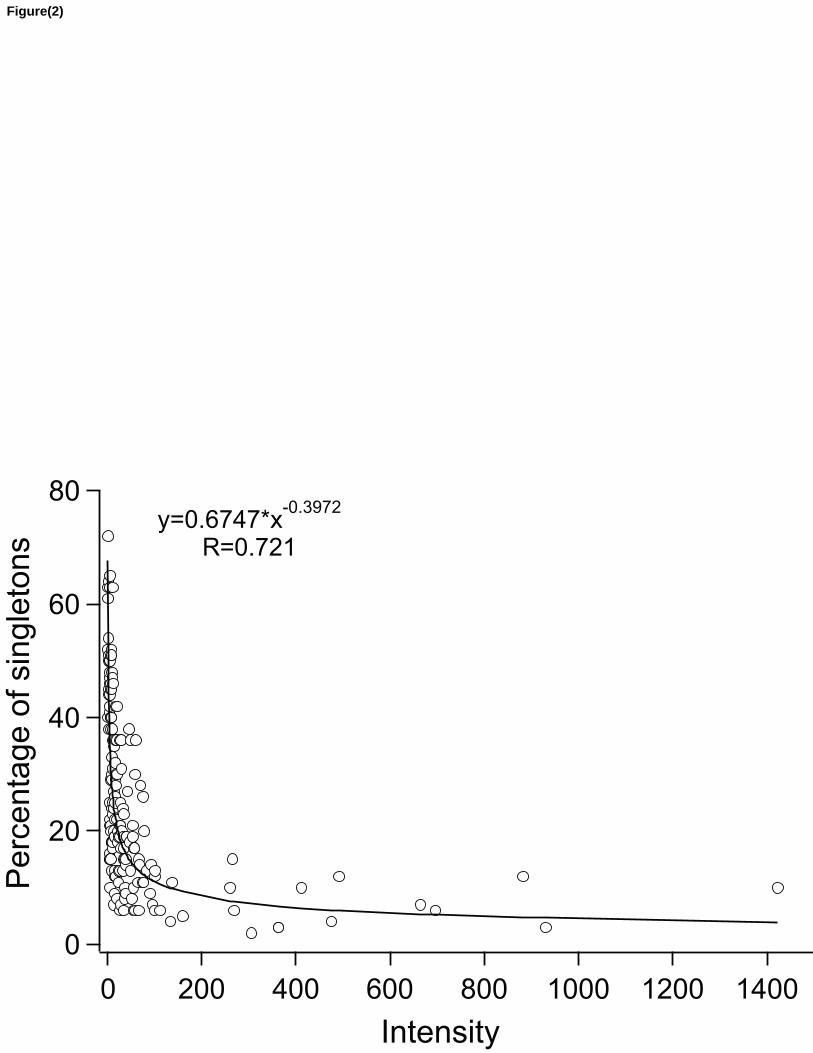
Our expanded database encompasses 185 communities, ranging from 1 to 1,423 ind/spp of 167

intensity and between 2% and 72% singletons. The median intensity was 20.3 and the median 168

percentage of singletons 19.2%. The communities samples belonged to four major groups: 169

terrestrial vertebrates (n=79), terrestrial arthropods (n=72), corals (n=22) and trees (n=12) (see 170

Appendix S1). The correlation between intensity and percentage of singletons was highly 171

significant (log-transformed power curve, r= 0.72; p<0.0001; Fig. 2). The percentage of 172

9

singletons tended to decline as sampling intensity increased, with samples of intensity 5 or less 173

(n= 23) having an average of 46% singletons (±3% SE), while communities with a sampling 174

intensity of 100 or more (n= 20) had an average of 8% of singletons (±1% SE). Due to the shape 175

of the power curve, most of the reduction in singleton percentage occurred at lower intensities, 176

between 0 and 75 species/individuals. 177

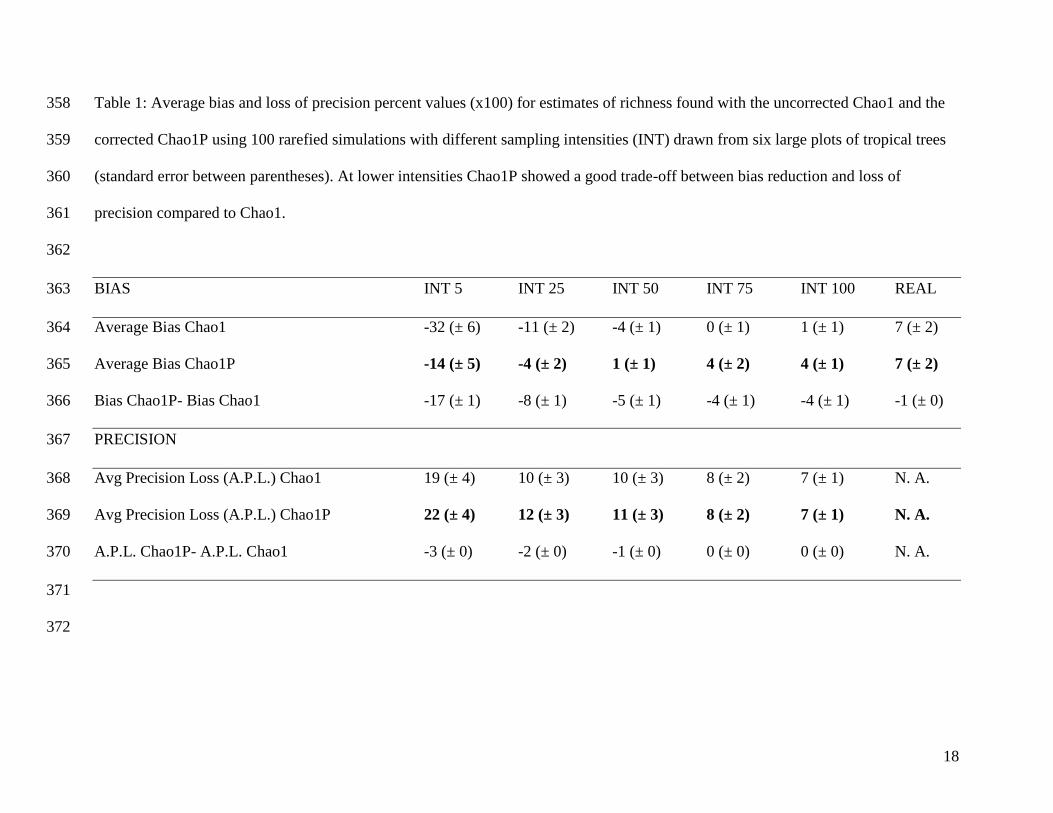
The Chao1P estimator had less bias and precision compared to Chao1, when tested in 178

rarefied sub-samples from six large plots of trees (Table 1). At higher intensities, both estimators 179

yield very similar results (0.8% on average bias difference at original intensities). However, at the 180

low intensity of 5 ind/spp, Chao1P outperforms Chao1 by 17.1% in terms of bias, with an 181

average precision loss of 2.8 % compared to Chao1 (Table 1). 182

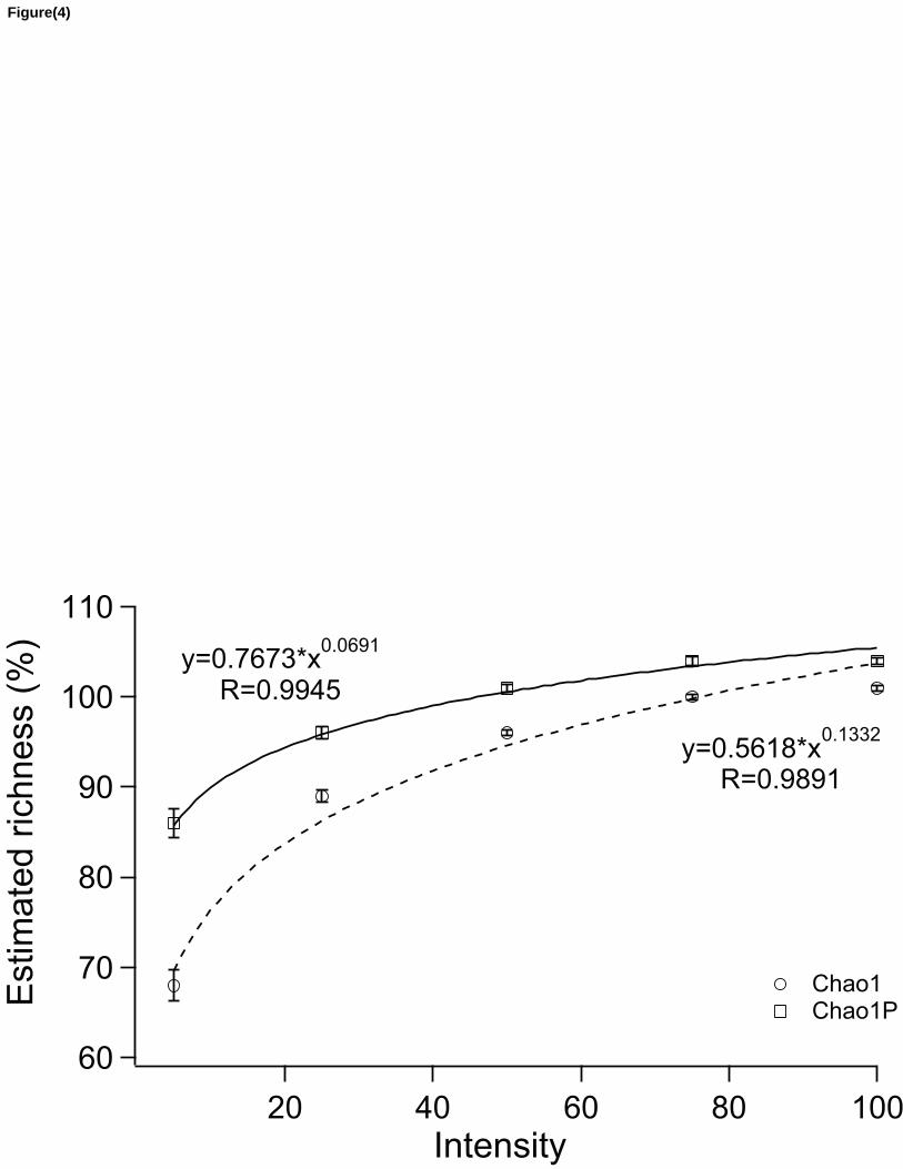
The estimated richness increased with rarefaction intensities in a pattern that fits very well 183

to the power curves for both Chao1P and Chao1 (R2 = 0.99 for Chao1P and 0.98 for Chao1) (Fig 184

4). These curves predict that, on average, Chao1P will estimate 100% of original richness at an 185

intensity of 52.0 ind/spp (± 9.4 SE), while Chao1 will reach 100% at an intensity of 78.7 ind/spp 186

(± 5.5 SE) (Fig. 4). If we use 95% of original richness instead of 100% as a good approximation 187

of original richness (as proposed by Chao et al. (2009)), the thresholds change to 20.7 ind/spp (± 188

5.9 SE) for Chao1P and 50.0 ind/spp (± 9.4 SE) for Chao1. 189

The difference between the two estimators obtained from the rarefaction simulations (from 190

tree plots with intensity 261 or more) showed good agreement with the average difference 191

obtained from samples of taxa that had low intensity (Fig.5). For example, on rarefactions to an 192

intensity of 5 the Chao1P estimates were, on average, 17.1% (± 1% SE) higher than Chao1 while 193

for the 57 communities (29 of arthropods and 28 of vertebrates) in our database with intensities 194

ranging between zero and 10 (midpoint intensity 5) the average difference was 17.2% (± 2% SE) 195

(Fig. 5). 196

10

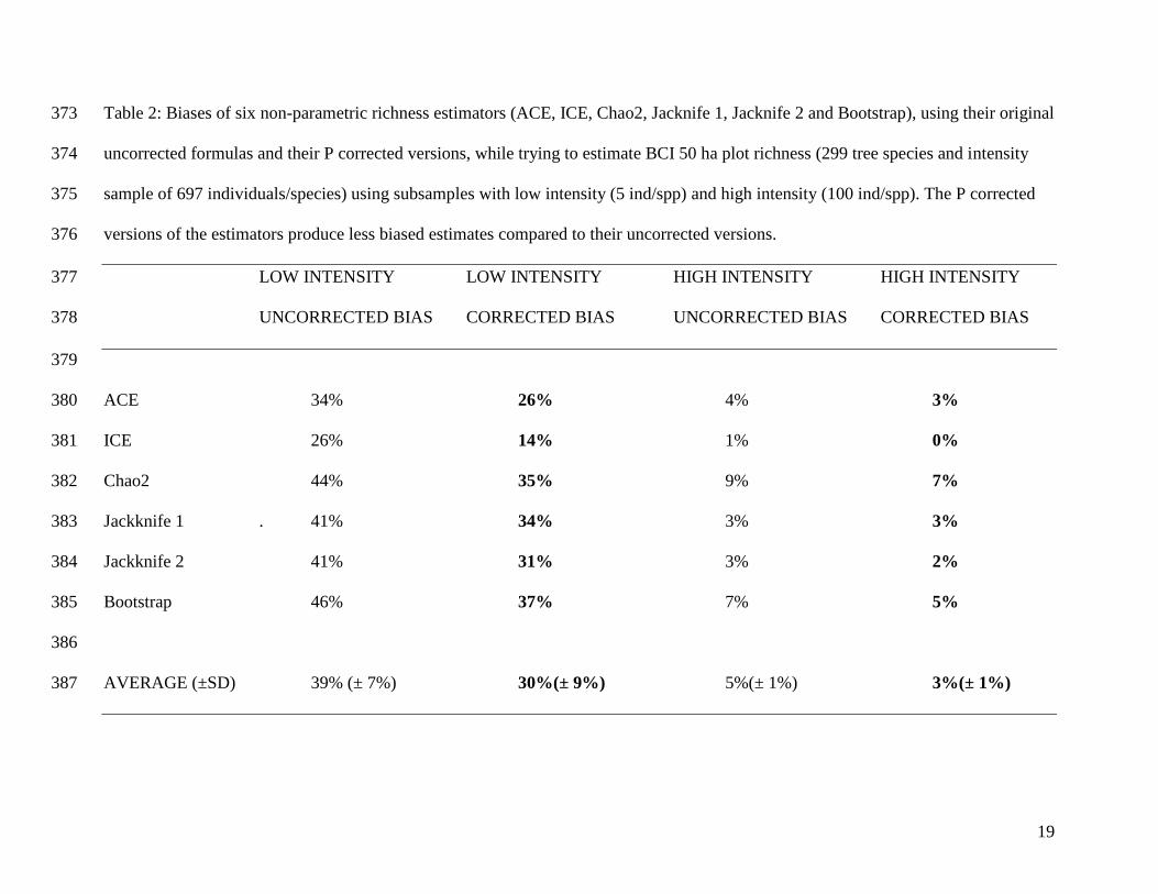
The P transformation improved the performance of the other 6 non-parametrical estimators 197

(Chao2, Jack1, Jack2, ACE, ICE and Bootstrap) in similar way it did for Chao1. The transformed 198

estimators produced estimates that were more close to BCI real richness compared to their 199

untransformed versions under simulated conditions of low sampling effort (9% less biased, in 200

average, compared to the uncorrected formulas at the intensity of 5 ind/spp) and converge to the 201

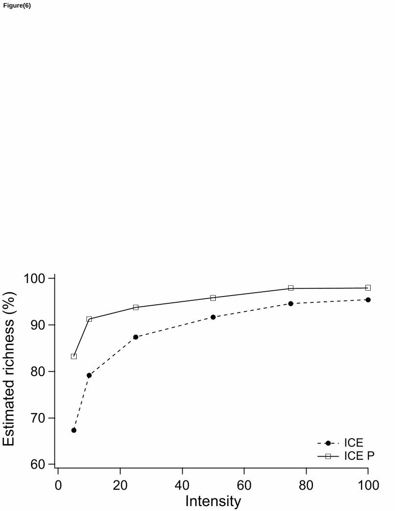
untransformed values as sampling effort increases (Table 2). The ICE corrected estimator 202

(“ICEP”) showed the best overall performance, in these simulations, estimating, in average, 83% 203

of BCI real richness at intensity 5 ind/spp compared to 67% made using its uncorrected version 204

(Fig. 6). 205

206

4. Discussion 207

208

Our expanded dataset confirmed the trend found by Coddington et al. (2009) for their 209

arthropod database: the percentage of singletons tends to decrease with an increase in the 210

sampling intensity in a very consistent way. At lower intensities, one needs to increase the 211

intensity of sampling by five-fold in order to halve the frequency of singletons. However, at 212

higher intensities (roughly, above intensity 100), the frequency of singletons tends to stabilize 213

around 8% (Fig. 2). Given that we have a phylogenetically diverse group of assemblages present 214

in our database (corals, arthropods, vertebrates and trees), we assume that this pattern is a general 215

one among communities. Consequently, the value of 8% (± 4% SD) is probably close to the 216

percentage of singletons expected from most natural communities after severe undersampling 217

bias is removed. 218

Since the proportion of singletons has a robust statistical relationship with the degree of 219

undersampling, it can be used to adjust the results from non-parametrical estimators. Our 220

11

transformation, empirically derived from this relationship, was able to reduce the bias from all 221

the non-parametric estimators tested compared to their untransformed versions at low sampling 222

intensities, while both versions (corrected x uncorrected) converged to very similar values at high 223

intensities. 224

The accuracy of an estimator is a compromise between the variation among estimations 225

(precision) and the distance between the estimated richness and the real richness (bias) (Brose et 226

al. 2003, Walther and Moore 2005). For example, at lower intensities (intensity 5), the corrected 227

Chao1P showed a reasonable trade-off, losing on average 3% precision, but gaining 17% in bias 228

reduction compared to Chao1. A mean of 17% less bias was found in both the rarefaction 229

simulations, drawn from high intensity samples, and from non-rarified lower intensity samples 230

(Fig. 5). This agreement between rarefied sub-samples from large tree plots and other multi-taxa 231

data suggests that the simulations were able to reproduce realistic patterns in low intensity 232

samples of natural situations. 233

Notice that the improvement provided by Chao1P applies not only to the average values but 234

also to the 95% boundary, which can be used to produce less conservative richness estimates. For 235

example, for the BCI dataset rarefied at an intensity of 5 ind/spp, Chao1P improved both the 236

average estimate (24% less bias) and the upper 95% estimate (26% less bias) compared to 237

untransformed Chao1. 238

The rarefactions, using data from six large plots of trees, also allows us to predict the 239

minimum intensity necessary for Chao1 and Chao1P to make estimates close to 100% of original 240

species richness. According to these simulations, it would be necessary to sample, on average, 241

51% more individuals to be able to make an accurate estimation using Chao1 (minimum intensity 242

78.7 ind/spp) compared to Chao1P (minimum intensity 52.0 ind/spp). A difference of this 243

12

magnitude can represent a great economy of time and resources while estimating the total 244

richness of very diverse communities. 245

If one uses 95% of the total richness estimated as a more tenable goal (Chao et al. 2009), 246

the difference in sampling effort between Chao1P and Chao1 becomes even larger, since our 247

simulations predict that one would need to sample, on average, 142% more individuals using 248

Chao1 (minimum intensity 50.0) than for Chao1P (minimum intensity 20.7) to estimate 95% of a 249

total sample richness. Since we found an increase of only 2% on Chao1P precision loss compared 250

to Chao1 at intensity 25 (close to the threshold of 20.7 for Chao1P for 95% estimation), the 251

trade-off between loss of precision and gain in economy of sampling effort in order to estimate 252

95% of total richness appears to be extremely positive. 253

The other non-parametric estimators tested (Chao2, Jack1, Jack2, ACE, ICE and Bootstrap) 254

presented the same pattern found with Chao1 (Fig. 6). The P corrected versions of each estimator 255

tested produced less biased estimates at low sampling intensities compared to their original 256

formulas while the corrected values converge to the original ones as the intensity of sampling 257

increases. The corrected version of ICE (ICEP), for example, was able to estimate 95% of BCI 258

plot using sub-samples with 50 ind/spp of intensity while the uncorrected version of ICE only 259

achieved the same feat at intensity 100 ind/spp (Fig. 6), this difference represents an economy of 260

50% in terms of sampling effort. 261

Consequently, our findings strongly indicate that our correction for non-parametric 262

estimators (equation (3)) produce less biased results and should be used to estimate the richness 263

in ecological studies that are trying to remove the effects of undersampling. An alternative option 264

is to parametric extrapolate the number of species to a given area or number of individuals (Melo 265

et al. 2007, O'Dea et al. 2006, Reichert et al. 2010). However, if such information (the total 266

13

community area, or the final number of individuals expected to be sampled) is not available, a 267

non-parametrical estimation using the correction present in equation (3) is the best option. 268

We also demonstrated that the intensity of sampling (the number of individuals sampled 269

divided by the number of species) and the proportion of singletons (the number of species 270

represented by one individual divided by the total number of species) can be used to indirectly 271

access the accuracy of richness estimates. Since these two parameters can be easily determined at 272

each stage of a real sampling program they can provide useful guidelines for planning and 273

evaluating biodiversity surveys. In our multi-taxa database, for example, 74% of the inventories 274

are below the average intensity threshold necessary to estimate at least 95% of the total richness 275

using Chao1, and 50% did not reach the same kind of threshold for Chao1P. These numbers give 276

support to Coddington et al.’s (2009) arguments that we need greater investment in biodiversity 277

inventories in order to get a realistic picture of the true richness of highly diverse ecosystems. 278

Our results indicate that ecological surveys that present more than 8% of singletons, or less 279

than 100 individuals/species of sampling intensity, probably are suffering from some degree of 280

undersampling and could be improved either by an increase of sampling effort or by using 281

richness estimators. Our simulations and database analysis led us to recommend the threshold of 282

20 individuals/species, or less than 21% of singletons, as a minimum sampling effort to produce 283

reliable richness estimates (at least 95% of richness estimated) using corrected non-parametric 284

estimators. This threshold rise for 50 individuals/species, or less than 14% of singletons, if non-285

corrected estimators are used, which implies in an economy of 60% of sampling effort due to the 286

correction factor. 287

288

289

14

Acknowledgments 290

We thank Nicholas Gotelli, Adriano S. Melo and Carlos Eduardo Grelle for insightful 291

comments on the subject.This work is supported by research fellowship from CNPq to DOM and 292

a post doc fellowship from CNPq/FAPESQ to MPAF. 293

294

15

References 295

296

Brose, U.,Martinez, N. D. 2004. Estimating the richness of species with variable mobility. Oikos 297

105(2), 292-300. 298

Burnham, K. P.,Overton, W. S. 1978. Estimation of the size of a closed population when capture 299

probabilities vary among animals. Biometrika 65, 623–633 300

Chao, A. 1984. Nonparametric-estimation of the number of classes in a population. Scandinavian 301

Journal of Statistics 11(4), 265-270. 302

Chao, A. 1987. Estimating the population size for capture-recapture data with unequal 303

catchability. Biometrics 437, 83-791. 304

Chao, A., Colwell, R. K., Lin, C. W.,Gotelli, N. J. 2009. Sufficient sampling for asymptotic 305

minimum species richness estimators. Ecology 90(4), 1125-1133. 306

Chao, A.,Lee, S. M. 1992. Estimating the number of classes via sample coverage. Journal of the 307

American Statistical Association 87210–217. 308

Chiarucci, A., Enright, N. J., Perry, G. L. W., Miller, B. P.,Lamont, B. B. 2003. Performance of 309

nonparametric species richness estimators in a high diversity plant community. Diversity 310

and Distributions 9(4), 283-295. 311

Clarke, K., Lewis, M.,Ostendorf, B. 2011. Additive partitioning of rarefaction curves: Removing 312

the influence of sampling on species-diversity in vegetation surveys. Ecological 313

Indicators 11(1), 132-139. 314

Coddington, J. A., Agnarsson, I., Miller, J. A., Kuntner, M.,Hormiga, G. 2009. Undersampling 315

bias: the null hypothesis for singleton species in tropical arthropod surveys. Journal of 316

Animal Ecology 78(3), 573-584. 317

Colwell, R. K. 2009. EstimateS: Statistical estimation of species richness and shared species from 318

samples. Version 8.2. User's Guide and application published at: 319

http://purl.oclc.org/estimates. 320

Condit, R. G., M. S. Ashton, H. Balslev, N. V. L. Brokaw, S. Bunyavejchewin, G. B. Chuyong, 321

Co, L., H. S. Dattaraja, S. J. Davies, S. Esufali, C. E. N. Ewango, R. B. Foster, N. 322

Gunatilleke, S. Gunatilleke, C. Hernandez, S. P. Hubbell, R. John, D. Kenfack, S. 323

Kiratiprayoon, P. Hall, T. H. Hart, A. Itoh, J. V. LaFrankie, I. Liengola, D. Lagunzad, S. 324

Lao, E. C. Losos, E. Magard, J. R. Makana, N. Manokaran, H. Navarrete, S. Mohammed 325

16

Nur, T. Okhubo, R. Perez, C. Samper, L. H. Hua Seng, R. Sukumar, J. C. Svenning, S. 326

Tan, D. W. Thomas, J. D. Thompson, M. I. Vallejo, G. Villa Muñoz, R. Valencia, T. 327

Yamakura,Zimmerman., J. K. 2005. Tropical tree α -diversity: Results from a worldwide 328

network of large plots. Biologiske Skrifter 55, 565-582. 329

CTFS 2009. Center for Tropical Forest Science.[WWW document]. URL http://www.ctfs.si.edu/. 330

Gotelli, N. J.,Colwell, R. K. 2001. Quantifying biodiversity: procedures and pitfalls in the 331

measurement and comparison of species richness. Ecology Letters 4(4), 379-391. 332

Heltshe, J. F.,Forrester, N. E. 1983. Estimating species richness using the Jackknife procedure. 333

Biometrics 3, 91–11. 334

Mao, C. X.,Colwell, R. K. 2005. Estimation of species richness: Mixture models, the role of rare 335

species, and inferential challenges. Ecology 86(5), 1143-1153. 336

Melo, A. S., Bini, L. M.,Thomaz, S. M. 2007. Assessment of methods to estimate aquatic 337

macrophyte species richness in extrapolated sample sizes. Aquatic Botany 86(4), 377-338

384. 339

O'Dea, N., Whittaker, R. J.,Ugland, K. I. 2006. Using spatial heterogeneity to extrapolate species 340

richness: a new method tested on Ecuadorian cloud forest birds. Journal of Applied 341

Ecology 43(1), 189-198. 342

Palmer, M. W. 1990. The estimation of species richness by extrapolation. Ecology 711195–1198. 343

Palmer, M. W. 1991. Estimating species richness: the second order jackknife reconsidered. 344

Ecology 72, 1512–1513. 345

Reichert, K., Ugland, K. I., Bartsch, I., Hortal, J., Bremner, J.,Kraberg, A. 2010. Species richness 346

estimation: estimator performance and the influence of rare species. Limnology and 347

Oceanography: Methods 8, 294-303. 348

Smith, E. P.,van Belle, G. 1984. Non-parametric estimation of species richness. Biometrics 40, 349

119–129. 350

Ulrich, W.,Ollik, M. 2005. Limits to the estimation of species richness: The use of relative 351

abundance distributions. Diversity and Distributions 11(3), 265-273. 352

Walther, B. A.,Moore, J. L. 2005. The concepts of bias, precision and accuracy, and their use in 353

testing the performance of species richness estimators, with a literature review of 354

estimator performance. Ecography 28(6), 815-829. 355

17

Zelmer, D. A.,Esch, G. W. 1999. Robust estimation of parasite component community richness. 356

Journal of Parasitology 85, 592–594. 357

18

Table 1: Average bias and loss of precision percent values (x100) for estimates of richness found with the uncorrected Chao1 and the 358

corrected Chao1P using 100 rarefied simulations with different sampling intensities (INT) drawn from six large plots of tropical trees 359

(standard error between parentheses). At lower intensities Chao1P showed a good trade-off between bias reduction and loss of 360

precision compared to Chao1. 361

362

BIAS INT 5 INT 25 INT 50 INT 75 INT 100 REAL 363

Average Bias Chao1 -32 (± 6) -11 (± 2) -4 (± 1) 0 (± 1) 1 (± 1) 7 (± 2) 364

Average Bias Chao1P -14 (± 5) -4 (± 2) 1 (± 1) 4 (± 2) 4 (± 1) 7 (± 2) 365

Bias Chao1P- Bias Chao1 -17 (± 1) -8 (± 1) -5 (± 1) -4 (± 1) -4 (± 1) -1 (± 0) 366

PRECISION 367

Avg Precision Loss (A.P.L.) Chao1 19 (± 4) 10 (± 3) 10 (± 3) 8 (± 2) 7 (± 1) N. A. 368

Avg Precision Loss (A.P.L.) Chao1P 22 (± 4) 12 (± 3) 11 (± 3) 8 (± 2) 7 (± 1) N. A. 369

A.P.L. Chao1P- A.P.L. Chao1 -3 (± 0) -2 (± 0) -1 (± 0) 0 (± 0) 0 (± 0) N. A. 370

371

372

19

Table 2: Biases of six non-parametric richness estimators (ACE, ICE, Chao2, Jacknife 1, Jacknife 2 and Bootstrap), using their original 373

uncorrected formulas and their P corrected versions, while trying to estimate BCI 50 ha plot richness (299 tree species and intensity 374

sample of 697 individuals/species) using subsamples with low intensity (5 ind/spp) and high intensity (100 ind/spp). The P corrected 375

versions of the estimators produce less biased estimates compared to their uncorrected versions. 376

LOW INTENSITY LOW INTENSITY HIGH INTENSITY HIGH INTENSITY 377

UNCORRECTED BIAS CORRECTED BIAS UNCORRECTED BIAS CORRECTED BIAS 378

379

ACE 34% 26% 4% 3% 380

ICE 26% 14% 1% 0% 381

Chao2 44% 35% 9% 7% 382

Jackknife 1 . 41% 34% 3% 3% 383

Jackknife 2 41% 31% 3% 2% 384

Bootstrap 46% 37% 7% 5% 385

386

AVERAGE (±SD) 39% (± 7%) 30%(± 9%) 5%(± 1%) 3%(± 1%) 387

20

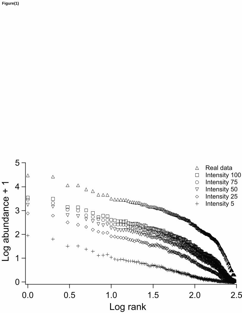
Figure 1: Abundance (log10) of tree species from BCI utilizing real data (census 2005, real 388

intensity 697 ind/spp) and the abundance averages from 100 rarefaction simulations under five 389

sampling intensities (100, 75, 50, 25 and 5 ind/spp). 390

391

Figure 2: Scatterplot between percentage sampling intensity (ind/spp) and percentage of 392

singletons for 185 communities belonging to 4 major taxa (arthropods, corals, trees and 393

vertebrates). The percentage of singletons falls sharply between 0 and 75 ind/spp, but tends to 394

stabilize around 8% singletons above intensity 100. 395

396

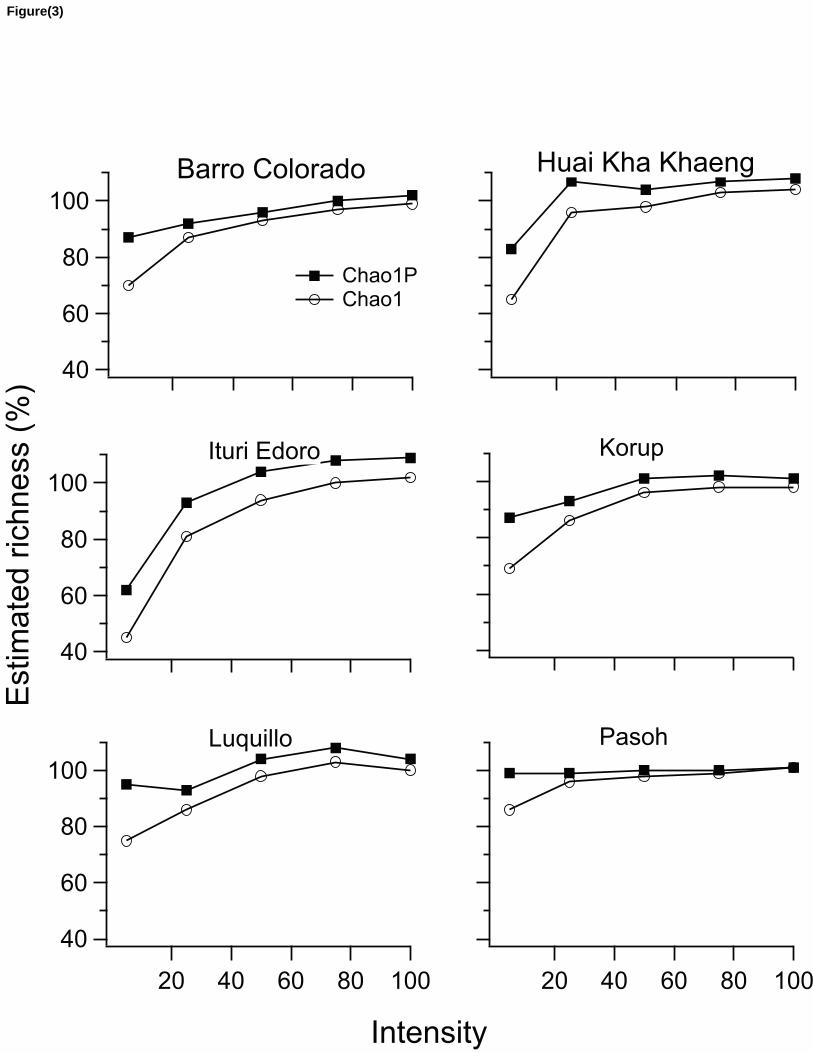
Figure 3: Average percentage of original richness estimated with uncorrected Chao1 and 397

corrected Chao1P estimators from rarified simulations with different sampling intensity efforts. 398

At higher intensities, both estimators tend to converge, but Chao1P estimates approaches faster 399

than Chao1 toward 100% of estimation as intensity increased in the six large plots of trees used 400

in the simulations. 401

402

Fig 4- Mean richness (SE bars) estimated by Chao1 and Chao1P estimators obtained from 403

rarefactions of six large plots of tropical trees. The fitted power curves were used to calculate the 404

minimum intensity necessary to estimate 95% and 100% of original richness. Chao1P crosses 405

these thresholds (95% and 100%) with less sampling effort than Chao1. 406

407

Figure 5: Average differences (SE bars) between Chao1 and Chao1P estimates for rarefactions 408

extracted from high intensity samples compared to differences obtained from real samples with 409

original low intensities. The pattern of improved estimation by Chao1P at low intensities 410

21

followed by convergence at higher intensities is very similar between rarefaction simulations and 411

real data. 412

Figure 6 : Comparative performance between corrected (ICEP) and uncorrected (ICE) version of 413

the ICE non-parametric richness estimator trying to predict the richness of BCI 50 ha plot (census 414

2005, richness= 299, intensity= 697 ind/spp). The corrected estimator produced less biased 415

estimates and make better predictions with less sampling effort. 416

5

4

3

2

1

0

2.52.01.51.00.50.0

Real data Intensity 100 Intensity 75 Intensity 50 Intensity 25 Intensity 5

Log rank

Lo

g a

bu

nd

an

ce

+ 1

Figure(1)

80

60

40

20

0

1400120010008006004002000

y=0.6747*x-0.3972

R=0.721

Intensity

Pe

rce

nta

ge

of sin

gle

ton

sFigure(2)

100

80

60

40

Chao1P Chao1

Barro Colorado

Huai Kha Khaeng

100

80

60

40

Ituri Edoro

Korup

10080604020

Pasoh

100

80

60

40

10080604020

Luquillo

Intensity

Estim

ate

d r

ich

ne

ss (

%)

Figure(3)

110

100

90

80

70

60

10080604020

Chao1 Chao1P

y=0.7673*x0.0691

R=0.9945

y=0.5618*x0.1332

R=0.9891

Intensity

Estim

ate

d r

ich

ne

ss (

%)

Figure(4)

20

15

10

5

0

10080604020

Real samples Rarefactions

Intensity

Estim

ate

s d

ife

ren

ce

(%

)Figure(5)

100

90

80

70

60

Estim

ate

d r

ich

ne

ss (

%)

100806040200

Intensity

ICE ICE P

Figure(6)

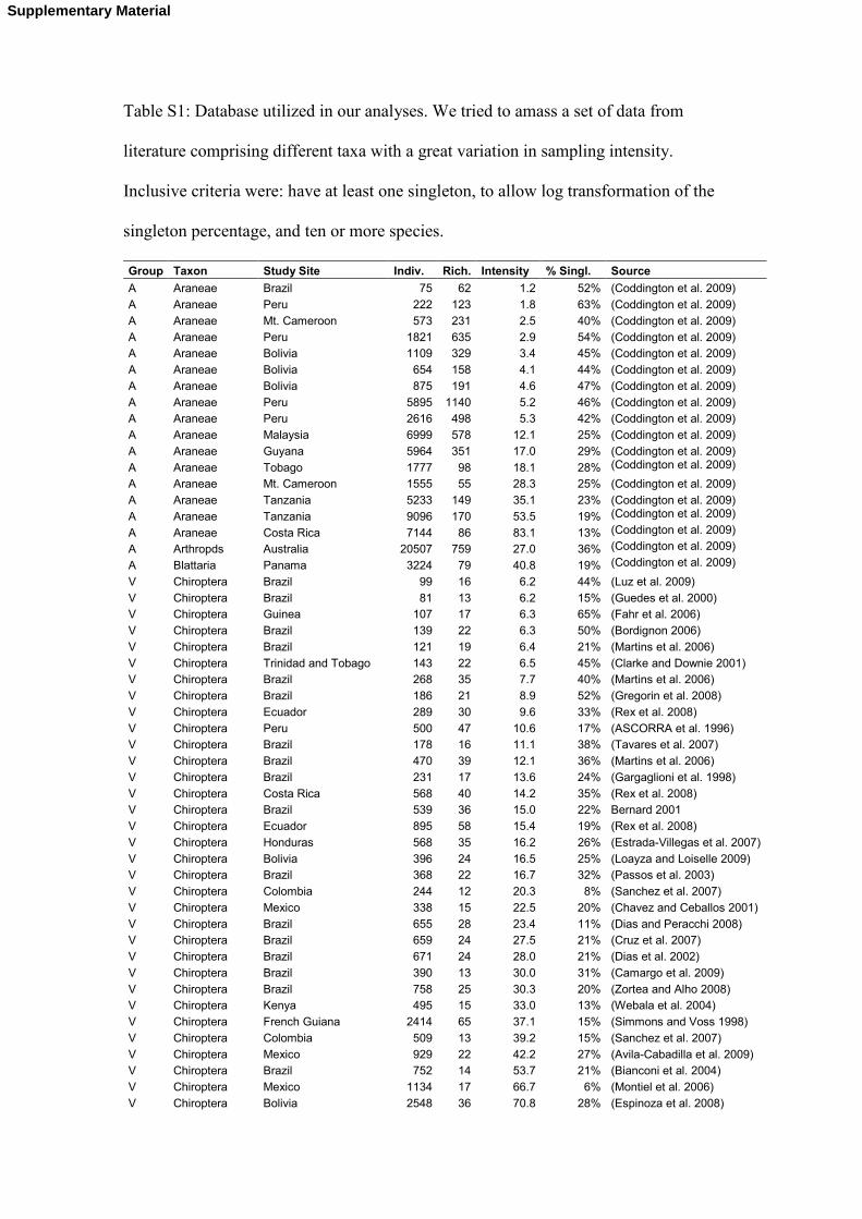
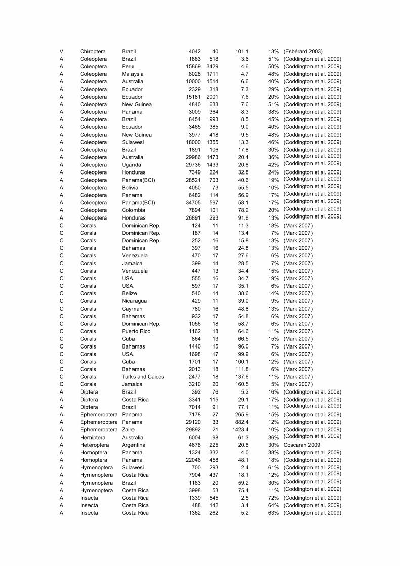
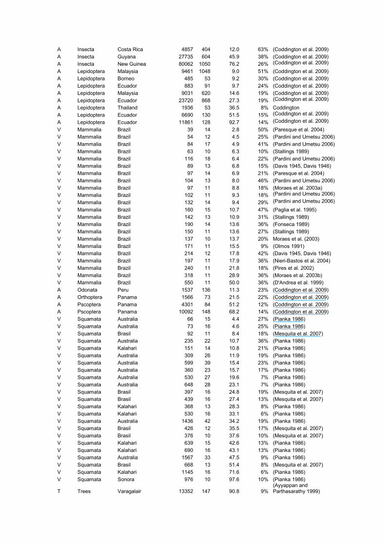
Table S1: Database utilized in our analyses. We tried to amass a set of data from

literature comprising different taxa with a great variation in sampling intensity.

Inclusive criteria were: have at least one singleton, to allow log transformation of the

singleton percentage, and ten or more species.

Group Taxon Study Site Indiv. Rich. Intensity % Singl. Source

A Araneae Brazil 75 62 1.2 52% (Coddington et al. 2009)

A Araneae Peru 222 123 1.8 63% (Coddington et al. 2009)

A Araneae Mt. Cameroon 573 231 2.5 40% (Coddington et al. 2009)

A Araneae Peru 1821 635 2.9 54% (Coddington et al. 2009)

A Araneae Bolivia 1109 329 3.4 45% (Coddington et al. 2009)

A Araneae Bolivia 654 158 4.1 44% (Coddington et al. 2009)

A Araneae Bolivia 875 191 4.6 47% (Coddington et al. 2009)

A Araneae Peru 5895 1140 5.2 46% (Coddington et al. 2009)

A Araneae Peru 2616 498 5.3 42% (Coddington et al. 2009)

A Araneae Malaysia 6999 578 12.1 25% (Coddington et al. 2009)

A Araneae Guyana 5964 351 17.0 29% (Coddington et al. 2009)

A Araneae Tobago 1777 98 18.1 28% (Coddington et al. 2009) A Araneae Mt. Cameroon 1555 55 28.3 25% (Coddington et al. 2009)

A Araneae Tanzania 5233 149 35.1 23% (Coddington et al. 2009)

A Araneae Tanzania 9096 170 53.5 19% (Coddington et al. 2009) A Araneae Costa Rica 7144 86 83.1 13% (Coddington et al. 2009) A Arthropds Australia 20507 759 27.0 36% (Coddington et al. 2009) A Blattaria Panama 3224 79 40.8 19% (Coddington et al. 2009) V Chiroptera Brazil 99 16 6.2 44% (Luz et al. 2009)

V Chiroptera Brazil 81 13 6.2 15% (Guedes et al. 2000)

V Chiroptera Guinea 107 17 6.3 65% (Fahr et al. 2006)

V Chiroptera Brazil 139 22 6.3 50% (Bordignon 2006)

V Chiroptera Brazil 121 19 6.4 21% (Martins et al. 2006)

V Chiroptera Trinidad and Tobago 143 22 6.5 45% (Clarke and Downie 2001)

V Chiroptera Brazil 268 35 7.7 40% (Martins et al. 2006)

V Chiroptera Brazil 186 21 8.9 52% (Gregorin et al. 2008)

V Chiroptera Ecuador 289 30 9.6 33% (Rex et al. 2008)

V Chiroptera Peru 500 47 10.6 17% (ASCORRA et al. 1996)

V Chiroptera Brazil 178 16 11.1 38% (Tavares et al. 2007)

V Chiroptera Brazil 470 39 12.1 36% (Martins et al. 2006)

V Chiroptera Brazil 231 17 13.6 24% (Gargaglioni et al. 1998)

V Chiroptera Costa Rica 568 40 14.2 35% (Rex et al. 2008)

V Chiroptera Brazil 539 36 15.0 22% Bernard 2001

V Chiroptera Ecuador 895 58 15.4 19% (Rex et al. 2008)

V Chiroptera Honduras 568 35 16.2 26% (Estrada-Villegas et al. 2007)

V Chiroptera Bolivia 396 24 16.5 25% (Loayza and Loiselle 2009)

V Chiroptera Brazil 368 22 16.7 32% (Passos et al. 2003)

V Chiroptera Colombia 244 12 20.3 8% (Sanchez et al. 2007)

V Chiroptera Mexico 338 15 22.5 20% (Chavez and Ceballos 2001)

V Chiroptera Brazil 655 28 23.4 11% (Dias and Peracchi 2008)

V Chiroptera Brazil 659 24 27.5 21% (Cruz et al. 2007)

V Chiroptera Brazil 671 24 28.0 21% (Dias et al. 2002)

V Chiroptera Brazil 390 13 30.0 31% (Camargo et al. 2009)

V Chiroptera Brazil 758 25 30.3 20% (Zortea and Alho 2008)

V Chiroptera Kenya 495 15 33.0 13% (Webala et al. 2004)

V Chiroptera French Guiana 2414 65 37.1 15% (Simmons and Voss 1998)

V Chiroptera Colombia 509 13 39.2 15% (Sanchez et al. 2007)

V Chiroptera Mexico 929 22 42.2 27% (Avila-Cabadilla et al. 2009)

V Chiroptera Brazil 752 14 53.7 21% (Bianconi et al. 2004)

V Chiroptera Mexico 1134 17 66.7 6% (Montiel et al. 2006)

V Chiroptera Bolivia 2548 36 70.8 28% (Espinoza et al. 2008)

Supplementary Material

V Chiroptera Brazil 4042 40 101.1 13% (Esbérard 2003)

A Coleoptera Brazil 1883 518 3.6 51% (Coddington et al. 2009)

A Coleoptera Peru 15869 3429 4.6 50% (Coddington et al. 2009)

A Coleoptera Malaysia 8028 1711 4.7 48% (Coddington et al. 2009)

A Coleoptera Australia 10000 1514 6.6 40% (Coddington et al. 2009)

A Coleoptera Ecuador 2329 318 7.3 29% (Coddington et al. 2009)

A Coleoptera Ecuador 15181 2001 7.6 20% (Coddington et al. 2009)

A Coleoptera New Guinea 4840 633 7.6 51% (Coddington et al. 2009)

A Coleoptera Panama 3009 364 8.3 38% (Coddington et al. 2009)

A Coleoptera Brazil 8454 993 8.5 45% (Coddington et al. 2009)

A Coleoptera Ecuador 3465 385 9.0 40% (Coddington et al. 2009)

A Coleoptera New Guinea 3977 418 9.5 48% (Coddington et al. 2009)

A Coleoptera Sulawesi 18000 1355 13.3 46% (Coddington et al. 2009)

A Coleoptera Brazil 1891 106 17.8 30% (Coddington et al. 2009)

A Coleoptera Australia 29986 1473 20.4 36% (Coddington et al. 2009) A Coleoptera Uganda 29736 1433 20.8 42% (Coddington et al. 2009) A Coleoptera Honduras 7349 224 32.8 24% (Coddington et al. 2009)

A Coleoptera Panama(BCI) 28521 703 40.6 19% (Coddington et al. 2009) A Coleoptera Bolivia 4050 73 55.5 10% (Coddington et al. 2009) A Coleoptera Panama 6482 114 56.9 17% (Coddington et al. 2009) A Coleoptera Panama(BCI) 34705 597 58.1 17% (Coddington et al. 2009) A Coleoptera Colombia 7894 101 78.2 20% (Coddington et al. 2009) A Coleoptera Honduras 26891 293 91.8 13% (Coddington et al. 2009) C Corals Dominican Rep. 124 11 11.3 18% (Mark 2007)

C Corals Dominican Rep. 187 14 13.4 7% (Mark 2007)

C Corals Dominican Rep. 252 16 15.8 13% (Mark 2007)

C Corals Bahamas 397 16 24.8 13% (Mark 2007)

C Corals Venezuela 470 17 27.6 6% (Mark 2007)

C Corals Jamaica 399 14 28.5 7% (Mark 2007)

C Corals Venezuela 447 13 34.4 15% (Mark 2007)

C Corals USA 555 16 34.7 19% (Mark 2007)

C Corals USA 597 17 35.1 6% (Mark 2007)

C Corals Belize 540 14 38.6 14% (Mark 2007)

C Corals Nicaragua 429 11 39.0 9% (Mark 2007)

C Corals Cayman 780 16 48.8 13% (Mark 2007)

C Corals Bahamas 932 17 54.8 6% (Mark 2007)

C Corals Dominican Rep. 1056 18 58.7 6% (Mark 2007)

C Corals Puerto Rico 1162 18 64.6 11% (Mark 2007)

C Corals Cuba 864 13 66.5 15% (Mark 2007)

C Corals Bahamas 1440 15 96.0 7% (Mark 2007)

C Corals USA 1698 17 99.9 6% (Mark 2007)

C Corals Cuba 1701 17 100.1 12% (Mark 2007)

C Corals Bahamas 2013 18 111.8 6% (Mark 2007)

C Corals Turks and Caicos 2477 18 137.6 11% (Mark 2007)

C Corals Jamaica 3210 20 160.5 5% (Mark 2007)

A Diptera Brazil 392 76 5.2 16% (Coddington et al. 2009)

A Diptera Costa Rica 3341 115 29.1 17% (Coddington et al. 2009)

A Diptera Brazil 7014 91 77.1 11% (Coddington et al. 2009) A Ephemeroptera Panama 7178 27 265.9 15% (Coddington et al. 2009)

A Ephemeroptera Panama 29120 33 882.4 12% (Coddington et al. 2009)

A Ephemeroptera Zaire 29892 21 1423.4 10% (Coddington et al. 2009)

A Hemiptera Australia 6004 98 61.3 36% (Coddington et al. 2009) A Heteroptera Argentina 4678 225 20.8 30% Coscaran 2009

A Homoptera Panama 1324 332 4.0 38% (Coddington et al. 2009)

A Homoptera Panama 22046 458 48.1 18% (Coddington et al. 2009)

A Hymenoptera Sulawesi 700 293 2.4 61% (Coddington et al. 2009)

A Hymenoptera Costa Rica 7904 437 18.1 12% (Coddington et al. 2009) A Hymenoptera Brazil 1183 20 59.2 30% (Coddington et al. 2009) A Hymenoptera Costa Rica 3998 53 75.4 11% (Coddington et al. 2009) A Insecta Costa Rica 1339 545 2.5 72% (Coddington et al. 2009)

A Insecta Costa Rica 488 142 3.4 64% (Coddington et al. 2009)

A Insecta Costa Rica 1362 262 5.2 63% (Coddington et al. 2009)

A Insecta Costa Rica 4857 404 12.0 63% (Coddington et al. 2009)

A Insecta Guyana 27735 604 45.9 38% (Coddington et al. 2009)

A Insecta New Guinea 80062 1050 76.2 26% (Coddington et al. 2009) A Lepidoptera Malaysia 9461 1048 9.0 51% (Coddington et al. 2009)

A Lepidoptera Borneo 485 53 9.2 30% (Coddington et al. 2009)

A Lepidoptera Ecuador 883 91 9.7 24% (Coddington et al. 2009)

A Lepidoptera Malaysia 9031 620 14.6 19% (Coddington et al. 2009)

A Lepidoptera Ecuador 23720 868 27.3 19% (Coddington et al. 2009) A Lepidoptera Thailand 1936 53 36.5 8% Coddington

A Lepidoptera Ecuador 6690 130 51.5 15% (Coddington et al. 2009) A Lepidoptera Ecuador 11861 128 92.7 14% (Coddington et al. 2009) V Mammalia Brazil 39 14 2.8 50% (Paresque et al. 2004)

V Mammalia Brazil 54 12 4.5 25% (Pardini and Umetsu 2006)

V Mammalia Brazil 84 17 4.9 41% (Pardini and Umetsu 2006)

V Mammalia Brazil 63 10 6.3 10% (Stallings 1989)

V Mammalia Brazil 116 18 6.4 22% (Pardini and Umetsu 2006)

V Mammalia Brazil 89 13 6.8 15% (Davis 1945, Davis 1946)

V Mammalia Brazil 97 14 6.9 21% (Paresque et al. 2004)

V Mammalia Brazil 104 13 8.0 46% (Pardini and Umetsu 2006)

V Mammalia Brazil 97 11 8.8 18% (Moraes et al. 2003a)

V Mammalia Brazil 102 11 9.3 18% (Pardini and Umetsu 2006) V Mammalia Brazil 132 14 9.4 29% (Pardini and Umetsu 2006) V Mammalia Brazil 160 15 10.7 47% (Paglia et al. 1995)

V Mammalia Brazil 142 13 10.9 31% (Stallings 1989)

V Mammalia Brazil 190 14 13.6 36% (Fonseca 1989)

V Mammalia Brazil 150 11 13.6 27% (Stallings 1989)

V Mammalia Brazil 137 10 13.7 20% Moraes et al. (2003)

V Mammalia Brazil 171 11 15.5 9% (Olmos 1991)

V Mammalia Brazil 214 12 17.8 42% (Davis 1945, Davis 1946)

V Mammalia Brazil 197 11 17.9 36% (Nieri-Bastos et al. 2004)

V Mammalia Brazil 240 11 21.8 18% (Pires et al. 2002)

V Mammalia Brazil 318 11 28.9 36% (Moraes et al. 2003b)

V Mammalia Brazil 550 11 50.0 36% (D'Andrea et al. 1999)

A Odonata Peru 1537 136 11.3 23% (Coddington et al. 2009)

A Orthoptera Panama 1566 73 21.5 22% (Coddington et al. 2009)

A Pscoptera Panama 4301 84 51.2 12% (Coddington et al. 2009)

A Pscoptera Panama 10092 148 68.2 14% (Coddington et al. 2009)

V Squamata Australia 66 15 4.4 27% (Pianka 1986)

V Squamata Australia 73 16 4.6 25% (Pianka 1986)

V Squamata Brasil 92 11 8.4 18% (Mesquita et al. 2007)

V Squamata Australia 235 22 10.7 36% (Pianka 1986)

V Squamata Kalahari 151 14 10.8 21% (Pianka 1986)

V Squamata Australia 309 26 11.9 19% (Pianka 1986)

V Squamata Australia 599 39 15.4 23% (Pianka 1986)

V Squamata Australia 360 23 15.7 17% (Pianka 1986)

V Squamata Australia 530 27 19.6 7% (Pianka 1986)

V Squamata Australia 648 28 23.1 7% (Pianka 1986)

V Squamata Brasil 397 16 24.8 19% (Mesquita et al. 2007)

V Squamata Brasil 439 16 27.4 13% (Mesquita et al. 2007)

V Squamata Kalahari 368 13 28.3 8% (Pianka 1986)

V Squamata Kalahari 530 16 33.1 6% (Pianka 1986)

V Squamata Australia 1436 42 34.2 19% (Pianka 1986)

V Squamata Brasil 426 12 35.5 17% (Mesquita et al. 2007)

V Squamata Brasil 376 10 37.6 10% (Mesquita et al. 2007)

V Squamata Kalahari 639 15 42.6 13% (Pianka 1986)

V Squamata Kalahari 690 16 43.1 13% (Pianka 1986)

V Squamata Australia 1567 33 47.5 9% (Pianka 1986)

V Squamata Brasil 668 13 51.4 8% (Mesquita et al. 2007)

V Squamata Kalahari 1145 16 71.6 6% (Pianka 1986)

V Squamata Sonora 976 10 97.6 10% (Pianka 1986)

T Trees Varagalair 13352 147 90.8 9% (Ayyappan and Parthasarathy 1999)

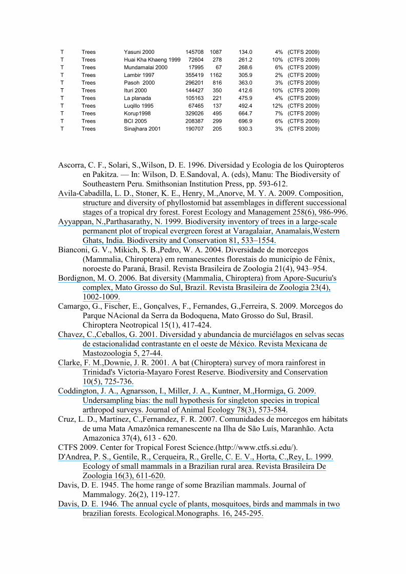
T Trees Yasuni 2000 145708 1087 134.0 4% (CTFS 2009)

T Trees Huai Kha Khaeng 1999 72604 278 261.2 10% (CTFS 2009)

T Trees Mundamalai 2000 17995 67 268.6 6% (CTFS 2009)

T Trees Lambir 1997 355419 1162 305.9 2% (CTFS 2009)

T Trees Pasoh 2000 296201 816 363.0 3% (CTFS 2009)

T Trees Ituri 2000 144427 350 412.6 10% (CTFS 2009)

T Trees La planada 105163 221 475.9 4% (CTFS 2009)

T Trees Luqillo 1995 67465 137 492.4 12% (CTFS 2009)

T Trees Korup1998 329026 495 664.7 7% (CTFS 2009)

T Trees BCI 2005 208387 299 696.9 6% (CTFS 2009)

T Trees Sinajhara 2001 190707 205 930.3 3% (CTFS 2009)

Ascorra, C. F., Solari, S.,Wilson, D. E. 1996. Diversidad y Ecologia de los Quiropteros

en Pakitza. — In: Wilson, D. E.Sandoval, A. (eds), Manu: The Biodiversity of

Southeastern Peru. Smithsonian Institution Press, pp. 593-612.

Avila-Cabadilla, L. D., Stoner, K. E., Henry, M.,Anorve, M. Y. A. 2009. Composition,

structure and diversity of phyllostomid bat assemblages in different successional

stages of a tropical dry forest. Forest Ecology and Management 258(6), 986-996.

Ayyappan, N.,Parthasarathy, N. 1999. Biodiversity inventory of trees in a large-scale

permanent plot of tropical evergreen forest at Varagalaiar, Anamalais,Western

Ghats, India. Biodiversity and Conservation 81, 533–1554.

Bianconi, G. V., Mikich, S. B.,Pedro, W. A. 2004. Diversidade de morcegos

(Mammalia, Chiroptera) em remanescentes florestais do município de Fênix,

noroeste do Paraná, Brasil. Revista Brasileira de Zoologia 21(4), 943–954.

Bordignon, M. O. 2006. Bat diversity (Mammalia, Chiroptera) from Apore-Sucuriu's

complex, Mato Grosso do Sul, Brazil. Revista Brasileira de Zoologia 23(4),

1002-1009.

Camargo, G., Fischer, E., Gonçalves, F., Fernandes, G.,Ferreira, S. 2009. Morcegos do

Parque NAcional da Serra da Bodoquena, Mato Grosso do Sul, Brasil.

Chiroptera Neotropical 15(1), 417-424.

Chavez, C.,Ceballos, G. 2001. Diversidad y abundancia de murciélagos en selvas secas

de estacionalidad contrastante en el oeste de México. Revista Mexicana de

Mastozoologia 5, 27-44.

Clarke, F. M.,Downie, J. R. 2001. A bat (Chiroptera) survey of mora rainforest in

Trinidad's Victoria-Mayaro Forest Reserve. Biodiversity and Conservation

10(5), 725-736.

Coddington, J. A., Agnarsson, I., Miller, J. A., Kuntner, M.,Hormiga, G. 2009.

Undersampling bias: the null hypothesis for singleton species in tropical

arthropod surveys. Journal of Animal Ecology 78(3), 573-584.

Cruz, L. D., Martínez, C.,Fernandez, F. R. 2007. Comunidades de morcegos em hábitats

de uma Mata Amazônica remanescente na Ilha de São Luís, Maranhão. Acta

Amazonica 37(4), 613 - 620.

CTFS 2009. Center for Tropical Forest Science.(http://www.ctfs.si.edu/).

D'Andrea, P. S., Gentile, R., Cerqueira, R., Grelle, C. E. V., Horta, C.,Rey, L. 1999.

Ecology of small mammals in a Brazilian rural area. Revista Brasileira De

Zoologia 16(3), 611-620.

Davis, D. E. 1945. The home range of some Brazilian mammals. Journal of

Mammalogy. 26(2), 119-127.

Davis, D. E. 1946. The annual cycle of plants, mosquitoes, birds and mammals in two

brazilian forests. Ecological.Monographs. 16, 245-295.

Dias, D.,Peracchi, A. L. 2008. Quirópteros da Reserva Biológica do Tinguá, estado do

Rio de Janeiro, sudeste do Brasil (Mammalia: Chiroptera). Revista Brasileira de

Zoologia 25(2), 333–369.

Dias, D., Peracchi, A. L.,Silva, S. S. P. 2002. Quirópteros do Parque Estadual da Pedra

Branca, Rio de Janeiro, Brasil (Mammalia, Chiroptera). Revista Brasileira de

Zoologia 19(Supl. 2), 113 - 140.

Esbérard, C. E. L. 2003. Diversidade de morcegos em área de Mata Atlântica

regenerada no sudeste do Brasil. Revista Brasileira de Zoociencias 5(2), 189-

204.

Espinoza, A. V., Aguirre, L. F., Galarza, M. I.,Gareca, E. 2008. Ensamble de

murciélagos en sitios con diferente grado de perturbación en un bosque montano

del parque nacional carrasco, Bolivia. Mastozoologia Neotropical 15(2), 297-

308.

Estrada-Villegas, S., Allen, L., García, M., Hoffmann, M.,Munroe, M. L. 2007. Bat

assemblage composition and diversity of the Cusuco National Park, Honduras.

Operation Wallacea, pp. 1-6.

Fahr, J., Djossa, B. A.,Vierhaus, H. 2006. Rapid assessment of bats (Chiroptera) in

Déré, Diécké and Mt. Béro classified forests, southeastern Guinea; including a

review of the distribution of bats in Guinée Forestière. — In: Wright, H.

E.McCullough, J.Alonso, L. E.Diallo, M. S. (eds), A Rapid Biological

Assessment of Three Classified Forests in Southeastern Guinea. Conservation

International, pp. 168-180, 245-47.

Fonseca, G. A. B. 1989. Small mammal species diversity in Brazilian tropical primary

and secundary forests of different sizes. Revista Brasileira.de Zoologia. 6(3),

381-422.

Gargaglioni, L. H., Batalhão, M. E., Lapenta, M. J., Carvalho, M. F., Rossi, R.

V.,Veruli, V. P. 1998. Mamíferos da Estação ecológica de Jataí, Luiz Antônio,

São Paulo. Papeis avulsos de zoologia 40(17), 267-287.

Gregorin, R., Capusso, G. L.,Furtado, V. R. 2008. Geographic distribution and

morphological variation in Mimon bennettii (Chiroptera, Phyllostomidae).

Iheringia Serie Zoologia 98(3), 404-411.

Guedes, P. G., Silva, S. S. P., Camardella, A. R., Abreu, M. F. G., Borges-Nojosa, D.

M., Silva, J. A. G.,Silva, A. A. 2000. Diversidade de mamíferos do parque

nacional de Ubajara (Ceará, Brasil). Mastozoologia Neotropical 7(2), 95-100.

Loayza, A. P.,Loiselle, B. A. 2009. COMPOSITION AND DISTRIBUTION OF A

BAT ASSEMBLAGE DURING THE DRY SEASON IN A NATURALLY

FRAGMENTED LANDSCAPE IN BOLIVIA. Journal of Mammalogy 90(3),

732-742.

Luz, J. L., Costa, L. M., Lourenço, E. C., Gomes, L. A. C.,Esbérard, C. E. L. 2009. Bats

from the Restinga of Praia das Neves, state of Espírito Santo, Southeastern

Brazil. Check List 5(2), 364–369.

Mark, K. W. 2007. AGRRA Database, version (10/2007).

(http://www.agrra.org/Release_2007-10/).

Martins, A. C. M., Bernard, E.,Gregorin, R. 2006. Rapid biological surveys of bats

(Mammalia, Chiroptera) in three conservation units in Amapa, Brazil. Revista

Brasileira de Zoologia 23(4), 1175-1184.

Mesquita, D. O., Colli, G. R.,Vitt, L. J. 2007. Ecological release in lizard assemblages

of neotropical savannas. Oecologia 153(1), 185-195.

Montiel, S., Estrada, A.,Leon, P. 2006. Bat assemblages in a naturally fragmented

ecosystem in the Yucatan Peninsula, Mexico: species richness, diversity and

spatio-temporal dynamics. Journal of Tropical Ecology 22, 267-276.

Moraes, L. B. d., Bossi, D. E. P.,Linhares, A. X. 2003a. Siphonaptera parasites of wild

rodents and marsupials trapped in three mountain ranges of the Atlantic Forest

in Southeastern Brazil. Memórias do Instituto Oswaldo Cruz 98(8), 1071-1076.

Moraes, L. B. d., Bossi, D. E. P.,Linhares, A. X. 2003b. Siphonaptera parasites of wild

rodents and marsupials trapped in three mountain ranges of the Atlantic Forest

in Southeastern Brazil. Memorias Do Instituto Oswaldo Cruz 98(8), 1071-1076.

Nieri-Bastos, F. A., Battesti, D. M. B., Linardi, P. M., Amaku, M., Marcili, A.,

Favorito, S. E.,Rocha, R. P. 2004. Ectoparasites on wild rodents from Parque

Estadual da Cantareira, SÆo Paulo, Brazil. Revista Brasileira de Parasitologia

Veterin ria 13(1), 29-35.

Olmos, F. 1991. Observations on the behavior and population dynamics of some

brazilian Atlantic Forest rodents. Mammalia. 55(4), 555-565.

Paglia, A. P., de Marco, J., Costa, F. M., Pereira, R. F.,Lessa, G. 1995. Heterogeneidade

estrutural e diversidade de pequenos mam¡feros em um fragmento de mata

secund ria de Minas Gerais, Brasil. Revista Brasileira.de Zoologia. 12(1), 67-79.

Pardini, R.,Umetsu, F. 2006. Pequenos mam¡feros nao-voadores da Reserva Florestal

do Morro Grande: distribuicao das especies e da diversidade em uma rea de

Mata Atlantica. Biota Neotropica (Online) 6

Paresque, R., Souza, W. P., Mendes, S. L.,Fagundes, V. 2004. Composicao cariotipica

da fauna de roedores e marsupiais de duas reas de Mata Atlantica do Espirito

Santo, Brasil. Boletim do Museu de Biologia Mello Leitao Nova Serie. 175-33.

Passos, F. C., Silva, W. R., Pedro, W. A.,Bonin, M. R. 2003. Frugivoria em morcegos

(Mammalia, Chiroptera) no Parque Estadual Intervales, sudeste do Brasil.

Revista Brasileira de Zoologia 20(3), 511–517.

Pianka, E. R. 1986. Ecology and Natural History of Desert Lizards: Analyses of the

Ecological Niche and Community Structure. Princeton Univ. Press.

Pires, A. S., Lira, P. K., Fernandez, F. A. S., Schittini, G. M.,Oliveira, L. C. 2002.

Frequency of movements of small mammals among Atlantic Coastal Forest

fragments in Brazil. Biological Conservation 108(2), 229-237.

Rex, K., Kelm, D. H., Wiesner, K., Kunz, T. H.,Voigt, C. C. 2008. Species richness and

structure of three Neotropical bat assemblages. Biological Journal of the

Linnean Society 94(3), 617-629.

Sanchez, F., Alvarez, J., Ariza, C.,Cadena, A. 2007. Bat assemblage structure in two dry

forests of Colombia: Composition, species richness, and relative abundance.

Mammalian Biology 72(2), 82-92.

Simmons, N. B.,Voss, R. S. 1998. The mammals of Paracou, French Guiana: A

neotropical lowland rainforest fauna part - 1. Bats. Bulletin of the American

Museum of Natural History(237), 1-219.

Stallings, J. R. 1989. Small mammal inventories in an eastern Brazilian park.

Bull.Florida State Mus.Biol.Sci. 34(4), 153-200.

Tavares, V. C., Perini, F. A.,Lombardi, J. A. 2007. The bat communities (Chiroptera) of

the Parque Estadual do Rio Doce, a large remnant of Atlantic Forest in

southeastern Brazil. Lundiana 8(1), 35-47.

Webala, P. W., Oguge, N. O.,Bekele, A. 2004. Bat species diversity and distribution in

three vegetation communities of Meru National Park, Kenya. African Journal of

Ecology 42(3), 171-179.

Zortea, M.,Alho, C. J. R. 2008. Bat diversity of a Cerrado habitat in central Brazil.

Biodiversity and Conservation 17(4), 791-805.