The relationship between monthly and seasonal South-west England rainfall anomalies and concurrent...

INTERNATIONAL JOURNAL OF CLIMATOLOGY

Int. J. Climatol. 22: 197–217 (2002)

Published online in Wiley InterScience (www.interscience.wiley.com). DOI: 10.1002/joc.726

THE RELATIONSHIP BETWEEN MONTHLY AND SEASONAL SOUTH-WESTENGLAND RAINFALL ANOMALIES AND CONCURRENT NORTH

ATLANTIC SEA SURFACE TEMPERATURESIAN D. PHILLIPS* and GLENN R. MCGREGOR

School of Geography and Environmental Sciences, The University of Birmingham, Edgbaston, Birmingham, B15 2TT, UK

Received 11 April 2001Revised 8 August 2001

Accepted 20 August 2001

ABSTRACT

This paper assesses the relationship between a regional index of rainfall (SWER) over Devon and Cornwall, South-westEngland, and concurrent gridded (5° × 5°) sea-surface temperature anomalies (SSTAs) for the North Atlantic–Europeandomain (10–70°N, 80°W–20°E) over the period 1950–97. Monthly and seasonal SSTA : SWER correlation fields arederived, and stepwise regression models are then constructed to specify SWER through SSTA variations. In particular,this paper emphasizes the importance of assessing all correlation matrices for field significance, an analysis stage thatis often ignored by many researchers. The most temporally reproducible signal is found between depressed SSTs to thewest of the British Isles and above-average rainfall over Devon and Cornwall, although this eastern Atlantic signal isby no means constant over time in terms of its location and spatial extent. Another distinctive feature of the anomalycorrelation maps is for locally significant positive SSTA : SWER associations to emerge at high latitudes (60–70°N) insummer and early autumn, e.g. Davis Strait, Norwegian Sea. Field significance testing reveals that seasonal SSTA : SWERcorrelation fields are statistically more robust than their monthly counterparts. This is demonstrated by the fact that theseasonal fields (excluding summer) all achieve field significance at the 0.1 level, whereas only five of the 12 monthlyfields (January, May, July, October and December) do so, suggesting that some of the locally significant SSTA : SWERcorrelations presented in this paper could have been obtained by merely correlating SWER with a random number series.Copyright 2002 Royal Meteorological Society.

KEY WORDS: South-west England; rainfall; sea-surface temperatures; North Atlantic–European domain; field significance; locallysignificant correlation; stepwise regression

1. INTRODUCTION

There are two distinguishing characteristics of the climatology of the South-west Peninsula of England:the winter rainfall maximum and the moderate seasonal temperature range. These characteristics are not onlyimportant for water resource management, but have also shaped the human geography of Devon and Cornwall,the two administrative counties that form the South-west Peninsula. For example, the equable temperatureregime, and thus mild winters, results in the region being a popular retirement destination.

As groundwater accounts for less than 10% of the area’s water resources, the region is highly dependentupon a seasonally consistent and reliable precipitation input if negative socio-economic and environmentalimpacts are to be avoided. Consequently, South-west England is prone to shorter duration droughtsthat arise from inadequate reservoir recharge during a single dry winter and spring (Jones and Lister,1998).

This hydro-climatological sensitivity is further compounded by an influx of visitors into the Peninsuladuring the summer holiday season, when rainfall totals are usually at their lowest and evaporation rates at their

* Correspondence to: Ian D. Phillips, School of Geography and Environmental Sciences, The University of Birmingham, Edgbaston,B15 2TT, UK; e-mail: [email protected]

Copyright 2002 Royal Meteorological Society

198 I. D. PHILLIPS AND G. R. MCGREGOR

highest. For example, 18.4 million tourists visited the West Country Tourist Board Region in 1997, contributing£3268 million to the region’s economy (ONS, 1999). This seasonal mismatch between precipitation input andwater demand must also be placed in the context of the 33% increase in average daily water demand between1977 and 1996 that has intensified the strains evident on the region’s water supply system. However, it isimportant to note that the rapid increase in water demand has not continued throughout the late 1990s and early21st century, as demand management and other mitigation measures have begun to curtail increases in demand(Marsh, personal communication). This trend is reflected in most other Western European countries too.

The precipitation climatology of South-west England is characterized by its variability at a variety oftemporal scales (Phillips and McGregor, 1998). Although attempts have been made at trying to understandthis variability by considering atmospheric circulation variations (Phillips, 2000; Phillips and McGregor,2001a,b), little work has been done on assessing the importance of other climate variables, such as seasurface temperature (SST). SSTs actively modify and sometimes amplify atmospheric processes (Palmer,1993), and are thus important in explaining precipitation anomalies (Mo and Paegle, 2000). It is thusmore realistic to view the surface climate as a manifestation of the behaviour of the ocean–atmospheresystem.

There appears to be evidence for an association between SST and rainfall variations over South-westEngland and the British Isles as a whole. Research into the relationship between the British climate andSST variations began in the 1960s. Unlike the globally complete sea temperature and ice data sets that existtoday (Parker et al., 1995), these early research efforts were hindered by information sources that were oftengeographically sparse, of limited record length and of questionable homogeneity.

One such early investigation into sea temperature–climate linkages was the Murray and Ratcliffe (1969)study of the 1968 summer, which was characterized by blocking anticyclones and the unusually high frequencyof northerly and easterly winds over the British Isles, especially during July and August 1968. A large area ofbelow-average SSTs to the south-east of Newfoundland accompanied the summer of 1968, a pattern that wasestablished in June 1968. To test whether this SST–climate linkage was real, as opposed to being a productof chance, Murray and Ratcliffe (1969) analysed 11 Julys that followed Junes that had similar SST patternsto June 1968. The pressure anomaly fields for these 11 Julys were broadly consistent with the 1968 pattern,suggesting that sea temperatures played some part in determining the weather conditions over the UK in Julyand August 1968.

In light of these positive research findings, Ratcliffe and Murray (1970) conducted a more comprehensiveanalysis of the associations between North Atlantic sea temperature and European pressure. Study results,which are quoted extensively by subsequent authors, revealed that European pressure was most sensitive tofluctuations in SST to the south of Newfoundland. Above (below) average SSTs in this area were linkedstatistically to below (above) average pressure over Europe in the following month. Ratcliffe and Murray(1970) explained these findings through variations in the latent and sensible heat fluxes from the oceanto the atmosphere: above (below) normal ocean surface temperatures increase (decrease) the transfer ofheat fluxes to the overlying atmosphere, thereby encouraging (suppressing) the development of Atlanticdepressions.

The 1990s has seen a resurgence of interest in SST–climate studies in the mid-latitude belt (Peng andMysak, 1993; Barnston, 1994; Barnston and Smith, 1996; Colman, 1997; Johansson et al., 1998; Colman andDavey, 1999). Compared with the 1960s, today’s researchers have the advantage of being able to draw uponglobally complete data sets that contain an additional 20 years of good-quality historical data.

Wilby (1998) has recently explored the utility of sea temperatures for downscaling general circulationmodel (GCM) output. Statistical downscaling schemes to date have concentrated almost exclusively onatmospheric circulation indices (Kilsby et al., 1998) or weather classification systems. In his study, Wilby(1998) investigated whether the use of seasonal North Atlantic SST anomalies in addition to daily vorticitywould provide more realistic scenarios of daily precipitation characteristics at two stations in the UK. Wilby(1998 : 174) concluded from his results that ‘there may be some merit in using the North Atlantic SST seriesas a downscaling predictor variable for sites in the UK’.

In light of this suggestion, and given the improved SST data base that now exists, a study whose aim is toinvestigate the association between SST and rainfall in South-west England, a hydro-climatologically sensitive

Copyright 2002 Royal Meteorological Society Int. J. Climatol. 22: 197–217 (2002)

SOUTH-WEST ENGLAND RAINFALL SST RELATIONSHIPS 199

region of Britain, is certainly justified. Furthermore, the results presented in this paper are unique in tworespects. Firstly, this study will describe SST centres of action in the context of monthly and seasonal rainfallanomalies over South-west England, a task that has not been attempted to date. Secondly, and important froma methodological angle, all correlations presented in this paper will be tested for field significance. Frequently,researchers have described spatial patterns of correlations without considering whether such correlations couldhave arisen merely by chance.

More specifically, the objectives of this paper are:

(i) to describe associations between monthly and seasonal values of a rainfall anomaly index for Devon andCornwall (South-west England rainfall : SWER) and concurrent variations in North Atlantic SST;

(ii) to test the monthly and seasonal correlation patterns for field significance; and(iii) to develop equations that efficiently describe variations in monthly and seasonal SWER values from

concurrent SST fluctuations.

In Section 2 of this paper, details regarding the study area are provided, emphasizing throughout theimportance of sea temperature variations. The data and methodology used in this study are described inSection 3, which includes a detailed account of the field significance testing procedure used. Study results arepresented in Section 4; the implications of the results and their relationship to previous studies are discussedin Section 5, before conclusions are drawn in Section 6.

2. STUDY AREA

Being completely surrounded by sea, which has a higher specific heat capacity compared with the adjoininglandmass (McIlveen, 1992), and warmed by the North Atlantic drift, South-west England has one of themost equable temperature climatologies in the British Isles. In western Cornwall, for example, the annualtemperature range between the warmest and coldest months is only 9 °C compared with the 14 °C range thatis often observed in central England (Perry, 1997).

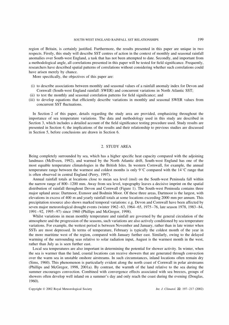
Annual rainfall totals at locations close to mean sea level (msl) on the South-west Peninsula fall withinthe narrow range of 800–1200 mm. Away from sea level, topography leaves a decisive imprint on the spatialdistribution of rainfall throughout Devon and Cornwall (Figure 1). The South-west Peninsula contains threemajor upland areas: Dartmoor, Exmoor and Bodmin Moor. Of these three areas, Dartmoor is the largest, withelevations in excess of 400 m and yearly rainfall totals at some locations exceeding 2000 mm per annum. Thisprecipitation resource also shows marked temporal variations: e.g. Devon and Cornwall have been affected byseven major meteorological drought events (winter 1962–63, 1964–65, 1975–76, late season 1978, 1983–84,1991–92, 1995–97) since 1960 (Phillips and McGregor, 1998).

Whilst variations in mean monthly temperature and rainfall are governed by the general circulation of theatmosphere and the progression of the seasons, such variations are also actively conditioned by sea temperaturevariations. For example, the wettest period is between November and January, rather than in late winter whenSSTs are most depressed. In terms of temperature, February is typically the coldest month of the year inthe more maritime west of the region, compared with January further east. Similarly, owing to the delayedwarming of the surrounding seas relative to solar radiation input, August is the warmest month in the west,rather than July as is seen further east.

Local sea temperatures are also important in determining the potential for shower activity. In winter, whenthe sea is warmer than the land, coastal locations can receive showers that are generated through convectionover the warm sea in unstable onshore airstreams. In such circumstances, inland locations often remain dry(Sims, 1960). This phenomenon is particularly evident along the north coast of Cornwall in polar airstreams(Phillips and McGregor, 1998, 2001a). By contrast, the warmth of the land relative to the sea during thesummer encourages convection. Combined with convergence effects associated with sea breezes, groups ofshowers often develop well inland on a summer’s day and only reach the coast during the evening (Douglas,1960).



Chivenor

Pr incetown

St Mawgan

Culdrose

DEVON

CORNWALL

0 40 Mi les

60 Ki lometres0

N

1200

800

1200

1000

1000

1400 1000

1800

1400

12001000

2000

2000

1800

16001400

1200

1000

1000

800

1000

1000

800

1000

800

1000

1000

1000

1000

1200

18001600

1400

1200

Figure 1. Mean annual rainfall (1961–90) over the South-west Peninsula of England and the location of rainfall stations used in thisstudy

Anomalous sea temperatures have the ability to perpetuate and amplify weather anomalies. One example ofthis mechanism in operation was the exceptionally wet conditions that affected Devon and Cornwall, togetherwith much of England and Wales, in September and October 1976 following the 1975–76 drought event(Doornkamp et al., 1980). When this drought event terminated in late August 1976, an upper-level troughreplaced the upper ridge that had dominated Britain’s weather throughout the summer of 1976. Ratcliffe(1977) argued that this circulation change was inadequate to explain the high rainfall totals that occurredover the subsequent two months. He suggested that the high sea temperatures that had developed during thevery warm summer offered a possible explanation. Enhanced evaporation rates over the ocean during thesummer drought added more moisture into the lower layers of the atmosphere. This moisture source was thenprecipitated out when the upper level circulation became favourable for rainfall generation in late August1976 and through the autumn of that year. Ratcliffe (1977) also noted how a strong north-west to south-eastSST gradient enhanced the baroclinicity ahead of the upper trough, and so led to the development of moredepressions in the area.

Wilby et al. (in press) used area-average SST anomalies for the North Atlantic sector (40–60°N, 35°W–5°E)in combination with airflow indices and values of the North Atlantic oscillation (NAO) index (Hurrell, 1995)to specify daily rainfall characteristics (e.g. mean wet-day amount) at 93 UK meteorological stations. Two ofthese stations, Bude and Plymouth, are located on the South-west Peninsula. The most coherent and widespreadSST forcing of daily rainfall characteristics, especially dry-spell persistence, was evident during spring andautumn. For example, above (below) average SSTs in these two seasons were associated with longer (shorter)dry spells. In autumn, the SST forcing was particularly widespread across central and southern England,including Devon and Cornwall. In light of their findings, Wilby et al. (in press) chose to investigate ingreater detail the conditioning of spring precipitation at Bude in north Cornwall as a ‘best-case’ scenario. Allmodels were calibrated over the period 1961–75; the validation period was 1976–90. With respect to Bude,inclusion of the low-frequency SST parameter achieved greater skill in diagnosing daily rainfall propertieswhen compared with models conditioned solely by regional airflow indices. Wilby et al. (in press) thus found



South-west England to be one of the most sensitive areas of the UK to North Atlantic SST forcing. Thisprovides further justification for this study’s investigation into SST–rainfall associations over Devon andCornwall. In particular, such a study is further justified on the grounds that the strength of SST conditioningcan be highly site specific. The Bude results presented by Wilby et al. (in press) thus may or may not berepresentative of South-west England as a whole.

3. DATA AND METHODOLOGY

Daily rainfall data were obtained from the archives of the region’s water supply company South West Waterfor 12 stations in Devon and Cornwall. These 12 rainfall stations are used by South West Water to monitorthe current hydrological and water resource situation across Devon and Cornwall. Phillips and McGregor(2001a) also used this station network to analyse the relationship between daily rainfall and wind directionin the South-west Peninsula.

Data from four of these locations (Figure 1), St Mawgan, Princetown, Chivenor and Culdrose, will be usedin this paper’s investigation of SST–rainfall associations. These four stations were chosen on the basis of theirrecord lengths (Table I) and the fact that they occupy geographically contrasting locations on the Peninsula.No data were available at Chivenor from September 1974 to August 1980 or at Culdrose in 1994. Phillipsand McGregor (1998) described the variations in meteorological drought severity at these four locations since1950. The Princetown series was extended back, in terms of monthly totals, to January 1950 using data fromthe Monthly Weather Report (MWR) of the UK Meteorological Office (UKMO) and British Rainfall. Thehomogeneity of the four monthly time series was confirmed by computing the non-parametric Kruskal–WallisH statistic (Ebdon, 1985). Further details can be found in Phillips and McGregor (1998).

Monthly rainfall totals (millimetres) were expressed as anomalies relative to the respective 1961–90monthly mean; Chivenor’s mean monthly totals were abstracted from the MWR. The four time series ofanomalies created were used to compute a regional rainfall anomaly index (SWER) for Devon and Cornwall.Given that daily rainfall over the South-west Peninsula is largely coherent in space and time (Phillips, 2000),such an index will provide an adequate first approximation of monthly variations in the region’s rainfallreceipt. Phillips and McGregor (2001b) also used this index in an analysis of water vapour flux–rainfallassociations over South-west England.

SWER is defined as:

SWER = 100N∑

1

(X/X)

where X is the monthly rainfall anomaly at one station, X is the station’s mean annual rainfall and N isthe number of stations, in this case four. Summing quotients of monthly anomalies to mean annual rainfallis a valid procedure because the magnitude of the anomalies themselves is closely related to each station’smean annual rainfall total (Phillips, 2000). Calculating SWER for months which had missing data at one ofthe four stations will have had a negligible impact on the SWER series. For example, three- and four-station

Table I. Record lengths of the archived daily SouthWest Water data used in this study

Station Record starts Record finishes

St Mawgan January 1957 June 1997Princetown January 1967 June 1997Chivenor February 1949 July 1997Culdrose January 1957 June 1997



SWER series, calculated excluding and including Chivenor’s rainfall anomaly, were very strongly correlatedwith each other (r = 0.991, n = 354).

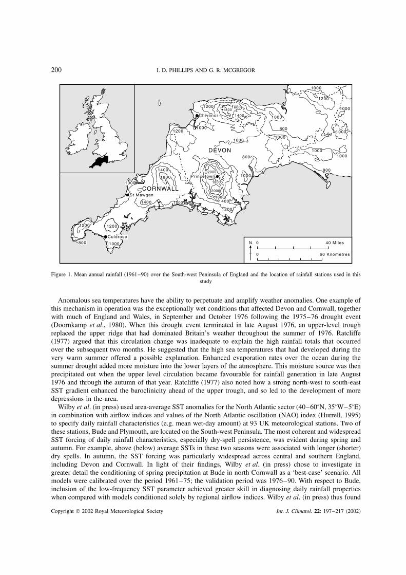
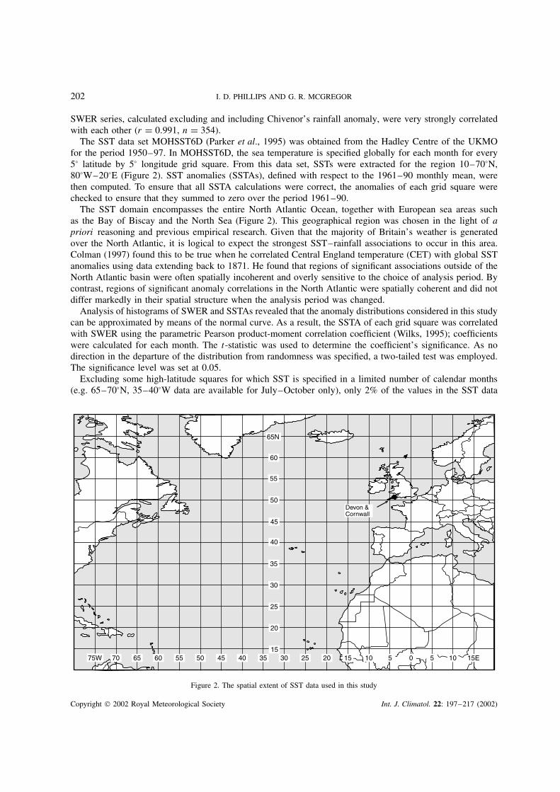
The SST data set MOHSST6D (Parker et al., 1995) was obtained from the Hadley Centre of the UKMOfor the period 1950–97. In MOHSST6D, the sea temperature is specified globally for each month for every5° latitude by 5° longitude grid square. From this data set, SSTs were extracted for the region 10–70°N,80°W–20°E (Figure 2). SST anomalies (SSTAs), defined with respect to the 1961–90 monthly mean, werethen computed. To ensure that all SSTA calculations were correct, the anomalies of each grid square werechecked to ensure that they summed to zero over the period 1961–90.

The SST domain encompasses the entire North Atlantic Ocean, together with European sea areas suchas the Bay of Biscay and the North Sea (Figure 2). This geographical region was chosen in the light of apriori reasoning and previous empirical research. Given that the majority of Britain’s weather is generatedover the North Atlantic, it is logical to expect the strongest SST–rainfall associations to occur in this area.Colman (1997) found this to be true when he correlated Central England temperature (CET) with global SSTanomalies using data extending back to 1871. He found that regions of significant associations outside of theNorth Atlantic basin were often spatially incoherent and overly sensitive to the choice of analysis period. Bycontrast, regions of significant anomaly correlations in the North Atlantic were spatially coherent and did notdiffer markedly in their spatial structure when the analysis period was changed.

Analysis of histograms of SWER and SSTAs revealed that the anomaly distributions considered in this studycan be approximated by means of the normal curve. As a result, the SSTA of each grid square was correlatedwith SWER using the parametric Pearson product-moment correlation coefficient (Wilks, 1995); coefficientswere calculated for each month. The t-statistic was used to determine the coefficient’s significance. As nodirection in the departure of the distribution from randomness was specified, a two-tailed test was employed.The significance level was set at 0.05.

Excluding some high-latitude squares for which SST is specified in a limited number of calendar months(e.g. 65–70°N, 35–40°W data are available for July–October only), only 2% of the values in the SST data

Devon &Cornwall

65N

60

55

50

45

40

35

30

25

20

1575W 70 65 60 55 50 45 40 35 30 25 20 15 10 5 0 5 10 15E

Figure 2. The spatial extent of SST data used in this study



matrices from January 1950 to December 1997 were missing. In particular, no data were available for June1972, September 1975 and July 1990. Given the low percentage of missing data, all correlation coefficientswere calculated using all available SSTA values; months with missing values for a particular grid square weresimply discarded from the analysis.

For each month, mean SSTAs were calculated for clusters of significant SSTA : SWER anomaly correla-tions. A cluster here is defined as being comprised of two or more 5° × 5° grid squares that share at leastone common edge or vertex. Cluster means (C1, C2, C3,. . ., Cn) were then used as the input variables intomultiple linear-regression models that specify SWER from SSTA. If no SSTA value was available for aparticular grid square in a given cluster, then the month’s SSTA cluster mean was computed using data fromthe remaining squares in the cluster. The stepwise option (Colman and Davey, 1999) was used to developan equation that describes variations in monthly SWER using mean SSTAs from the smallest number ofstatistically significant clusters possible.

There are a number of possible advantages of using local anomalies as the input (state) variables intomodels rather than principal components. Foremost, a low-dimensional state consisting of selected local valuesis easier to understand than principal components. Thacker and Lewandowicz (1997 : 3) noted: ‘Althoughprincipal components have the advantage of being uncorrelated, they are intrinsically non-local variablescharacterizing global patterns of correlations, and as such they contribute to the difficulties in interpreting thestatistical models in terms of regional effects’. Local and regional variables can thus be more easily relatedto physical processes.

Seasonal SSTA : SWER anomaly correlations were also calculated after all monthly sea temperature andrainfall anomalies had been summed across the respective season. This procedure creates seasonal values thathave a greater magnitude when compared with seasonal anomalies that are computed using the respective1961–90 seasonal mean. In this study, the standard climatological seasons were used: March–May (MAM);June–August (JJA); September–November (SON); December–February (DJF). Carrying out the analysesat the seasonal time frame is justified because SST–climate signals are often more evident at the three-monthly than the one-monthly time scale (Barnston, 1994), owing to the slow evolution of sea temperatureanomalies. The standard climatological seasons are merely artificial compartmentalizations of time rather thanobjectively existing entities. There are thus no a priori reasons to suggest that stronger SST conditioningwould not emerge if different combinations of months were used (e.g. JFM, OND) or indeed time periodsof, say, 4 or 5 months. The seasonal SST : SWER anomaly correlations presented in this paper are thus notnecessarily indicative of the strongest relationships that may be evident at the seasonal time scale.

Whilst any individual correlation coefficient may be statistically significant at the local 95% confidencelevel, there is still a possibility that such significant relationships have merely arisen by chance. For example,it is possible to obtain a statistically significant coefficient by simply correlating two random number series.To complete the significance testing, the spatial extent of the region of locally significant correlations must beassessed for field significance by considering the properties of finiteness and interdependence of the spatialgrid (Livezey and Chen, 1983). Some earlier studies (e.g. Colman and Davey, 1999; Wilby et al., in press)have not considered field significance.

Finiteness is defined as the dimensionality of the grid. There are two possible outcomes when calculatinga correlation coefficient for any given grid square: the coefficient is significant at the 95% confidence level(outcome a); the coefficient is not significant at the 95% confidence level (outcome b). This procedure isrepeated n times, where n is the number of grid squares in the data matrix. A two-outcome process (a + b)that is repeated n times has a binomial probability distribution. Examples of the binomial distribution arisingin everyday situations include the outcome of tossing a coin (head + tail) and drawing a heart from a standardpack of playing cards with replacement (heart + not a heart). The binomial expansion of (a + b)n can thus beused to determine the number of grid squares that must have statistically significant correlations at the 95%confidence level (Mo) from a total of n (the total number of correlation coefficients calculated) such that theprobability of the result occurring by chance is less than 0.05. Livezey and Chen (1983 : 49, figure 3) provideda graph in which this critical percentage (Mo) is given as a function of the number of tests n conducted.Mo is sensitive to n, decreasing as n increases. Owing to data availability, the number of independent testsconducted by month in this study ranges from 180 in March to 198 in August. Taking the lower of these two



figures, the critical value (Mo) for 180 independent tests can be estimated from Livezey and Chen’s (1983)diagram as being 8.0%. At least 8% of grid squares in any given month must, therefore, be locally significantfor the finiteness criterion for field significance to be satisfied at the 95% confidence level.

The finiteness criterion does not consider spatial interdependence in the grid. As SST is spatiallyautocorrelated, the number of degrees of freedom in the spatial field is reduced. For SSTA, suchautocorrelations are likely to be even more marked because the SSTs of some grid squares have simply beenextrapolated from neighbouring grid squares and do not represent data measurements per se. Furthermore,SSTs are specified for grid squares that contain only a small percentage of sea relative to land, suggestingthat these have also been merely extrapolated from adjoining squares.

The most likely outcome of strong interdependence in a spatial field is to increase the number of coefficientsthat are significant by chance. If one grid square is a ‘chance’ correlation, then neighbouring grid squaresare likely to be significant for the same reason. The finiteness criterion alone is thus inadequate for assessingfield significance in a spatially correlated data matrix.

Monte Carlo simulations are frequently employed to test for field significance in a spatially correlated datamatrix (Livezey and Chen, 1983; Wilks, 1995). Given that SSTAs exhibit strong autoregressive behaviour,which reduces the number of effective samples in the time series, the Monte Carlo simulations were conductedusing the January SSTA data only. SSTA data were available for 184 grid squares in the study area for January.

For the Monte Carlo simulation, the SWER series was replaced with a Gaussian noise series generated froma normal population whose mean and variance, N (0.159, 3.961), are identical to that of the SWER series overthe period January 1950 to June 1997. The ‘January’ values of this Gaussian noise series were then correlatedwith the January SSTA values of the 184 grid squares and the number of coefficients statistically significantat the 0.05 level noted. This procedure was repeated 200 times, using a new Gaussian noise series for eachsimulation in order to ensure that the probability distribution function was estimated adequately. A histogramwas constructed showing the number of statistically significant grid squares across the 200 trials from whichthe critical percentage Mo required for field significance at the 95% confidence level was estimated.

The assumption was thus made that the Monte Carlo simulations conducted using the January SSTA datawere representative of the results that would have been obtained if data from other months had been used.This assumption can be justified on the grounds that the calculation of anomalies has the effect of removingthe seasonal cycle from the data set. Nevertheless, researchers should feel free to experiment with differentcombinations of months for their simulations. Logical combinations include a winter and a summer month(e.g. January and July), and a month from each of the four seasons (e.g. January, April, July, October).

4. RESULTS

This section is divided into three parts. In Section 4.1 the spatial distribution of locally significant monthlySSTA : SWER anomaly correlations is described and tested for field significance. The seasonal results are thendescribed in Section 4.2, before the monthly and seasonal regression models are presented in Section 4.3.

4.1. Monthly SSTA : SWER anomaly correlations

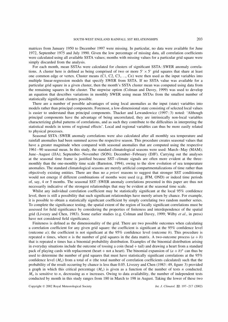
4.1.1. The spatial distribution of locally significant correlations. Dominating January’s anomaly correlationmap (Figure 3(a)) is a 20-cell contiguous cluster in the North Atlantic to the west of the British Isles between45 and 60°N. Correlation coefficients in this cluster ranged from −0.287 to −0.442. Above (below) averageSSTs in this region in January are thus significantly associated with below (average) rainfall over South-westEngland. This inverse North Atlantic cluster was evident in all months of the year (excluding June), albeitthat its geographic centre and spatial extent varied between individual months.

Positive SSTA : SWER associations (r = 0.324–0.450) were seen for the English Channel and southernNorth Sea in January and February (Figure 3(a) and (b)). Unlike the temporally consistent inverse NorthAtlantic signal, positive SSTA : SWER relationships were only found in this area in January and February.In February, a new region of positive anomaly correlations (r = 0.291–0.418) emerged over the Mediter-ranean (Figure 3(b)). This cluster was also seen during April (Figure 3(d)) and May (Figure 3(e)), with above



(below) average SSTs in this area being significantly related to above (below) average rainfall over Devonand Cornwall.

March’s significant anomaly correlation field (Figure 3(c)) differed markedly from adjacent months, withmost of the statistically significant associations occurring to the east of the British Isles. All of these sea areas(e.g. North Sea, Norwegian Sea) had SSTAs that were inversely related to March’s SWER, with r values ofbetween −0.294 and −0.547. An inverse signal was also seen over the North Sea in May (Figure 3(e)).

In May, a new region of significant anomaly correlations emerged to the south of Greenland (Figure 3(e)).This high-latitude positive signal was preserved during June (Figure 3(f)), July (Figure 3(g)) and August(Figure 3(h)). June had the lowest number of significant grid squares of any month (Figure 3(f)). Ofthe eight grid squares significant in June, all of which were geographically remote from the South-west Peninsula, five squares formed an inverse cluster to the south of Newfoundland, whilst theother three occurred in isolation, suggesting that their significant correlations may have arisen bychance.

Compared with June, more structure was evident in July’s anomaly correlation field (Figure 3(g)); 25 gridsquares were significant at the 0.05 level. Dominating the July map, as for most other months, was an inverse

(a)65N

60

55

50

45

40

35

30

25

20

1575W 70 65 60 55 50 45 40 35 30 25 20 10 5 0 5 10 15E15

Cluster 1

65N

60

55

50

45

40

35

30

25

20

1575W 70 65 60 55 50 45 40 35 30 25 20 10 5 0 5 10 15E15

Cluster 2

Cluster 1

Cluster 1

Cluster 3

Cluster 4

Cluster 2

Cluster 1

Cluster 3

50

45

40

35

30

25

20

1570 65 60 40 35 30 25 10 5 0 5 10 15E

65N

60

55

50

45

40

35

30

25

20

1575W 70 65 60 55 50 45 40 35 30 25 20 10 5 0 5 10 15E15

Cluster 2

Cluster 3

February65N

60

55

50

45

40

35

30

25

20

1575W 70 65 60 55 50 45 40 35 30 25 20 10 5 0 5 10 15E15

(b)

Cluster 1

Cluster 2

Cluster 3

65N

60

55

50

45

40

35

30

25

20

1575W 70 65 60 55 50 45 40 35 30 25 20 10 5 0 5 10 15E15

(c)

(d)

(e)

(f)

Cluster 1

Cluster 2

May

April

June

75W 55 50 45 20 15

55

60

65N

POSITIVE NEGATIVE

r < 0.4

r ≥ 0.4

r < -0.4

r ≤ -0.4

March

January

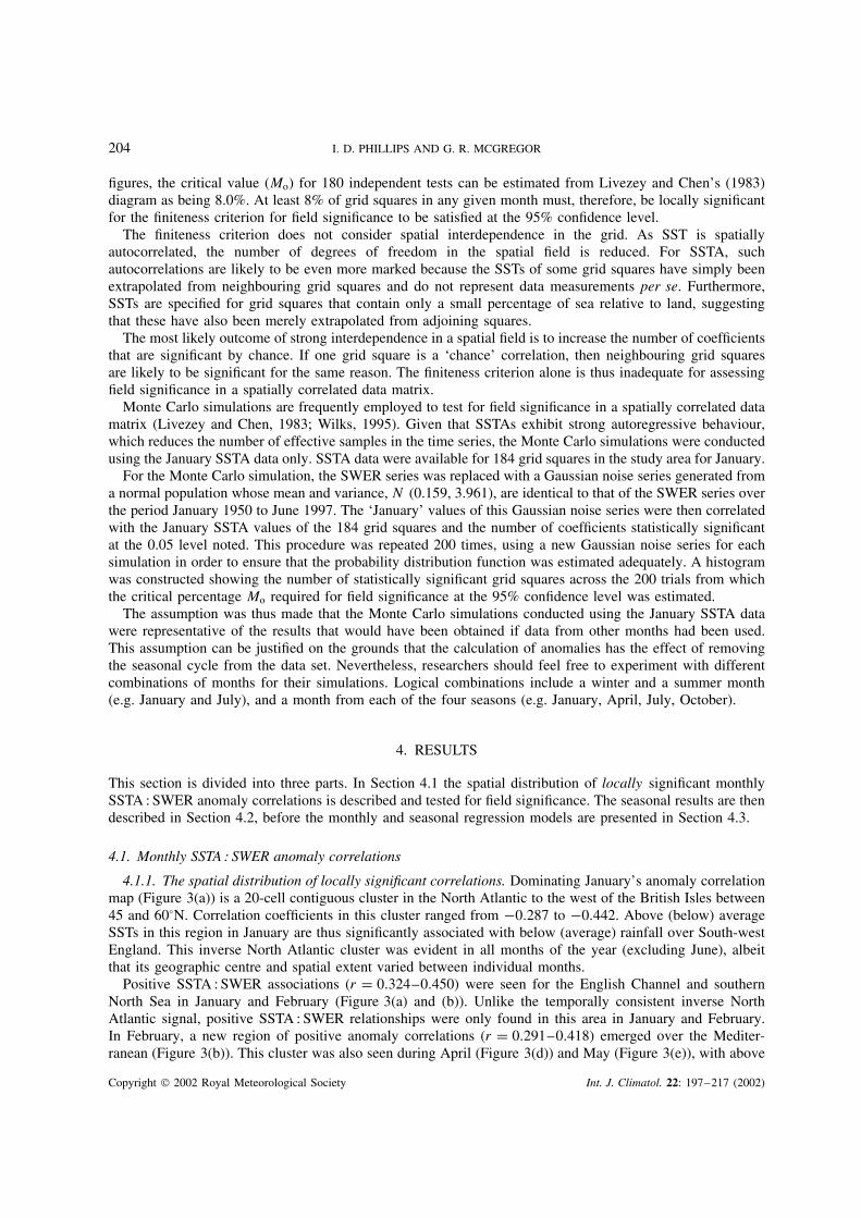
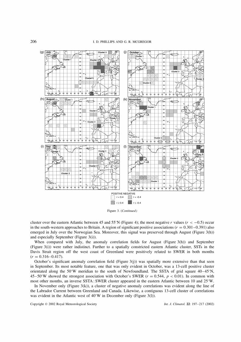
Figure 3. The spatial distribution of significant (p ≤ 0.05) monthly SSTA : SWER anomaly correlations: (a) January; (b) February;(c) March; (d) April; (e) May; (f) June; (g) July; (h) August; (i) September; (j) October; (k) November; (l) December



July(g)65N

60

55

50

45

40

35

30

25

20

1575W 70 65 60 55 50 45 40 35 30 25 20 10 5 0 5 10 15E15

Cluster 1

65N

60

55

50

45

40

35

30

25

20

1575W 70 65 60 55 50 45 40 35 30 25 20 10 5 0 5 10 15E15

Cluster 1

Cluster 1

Cluster 2

Cluster 3

Cluster 3

Cluster 1

Cluster 4

Cluster 3

Cluster 2

50

45

40

35

30

25

20

1570 65 60 40 35 30 25 10 5 0 5 10 15E

65N

60

55

50

45

40

35

30

25

20

1575W 70 65 60 55 50 45 40 35 30 25 20 10 5 0 5 10 15E15

Cluster 2

Cluster 3

Cluster 4

August65N

60

55

50

45

40

35

30

25

20

1575W 70 65 60 55 50 45 40 35 30 25 20 10 5 0 5 10 15E15

(h)

Cluster 3

Cluster 2

Cluster 4

Cluster 2

Cluster 1

Sep65N

60

55

50

45

40

35

30

25

20

1575W 70 65 60 55 50 45 40 35 30 25 20 10 5 0 5 10 15E15

(i)

(j)

(k)

(l)Cluster 1

Cluster 2

Cluster 3

Cluster 4

November

October

December

75W 55 50 45 20 15

55

60

65N

POSITIVE NEGATIVEr < 0.4

r ≥ 0.4

r < -0.4

r ≤ -0.4

Figure 3. (Continued)

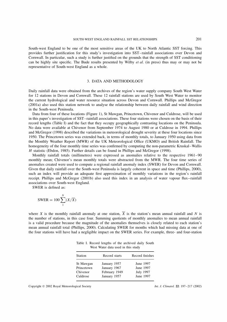
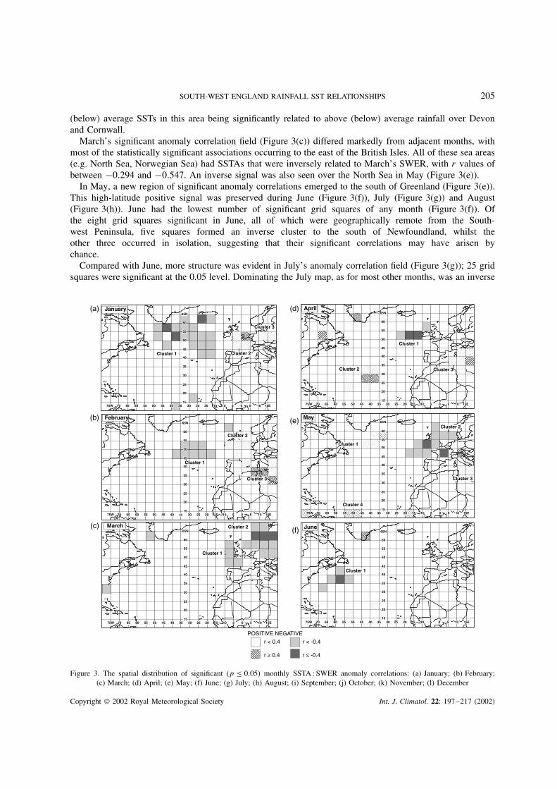
cluster over the eastern Atlantic between 45 and 55°N (Figure 4); the most negative r values (r < −0.5) occurin the south-western approaches to Britain. A region of significant positive associations (r = 0.301–0.391) alsoemerged in July over the Norwegian Sea. Moreover, this signal was preserved through August (Figure 3(h))and especially September (Figure 3(i)).

When compared with July, the anomaly correlation fields for August (Figure 3(h)) and September(Figure 3(i)) were rather indistinct. Further to a spatially constricted eastern Atlantic cluster, SSTs in theDavis Strait region off the west coast of Greenland were positively related to SWER in both months(r = 0.316–0.417).

October’s significant anomaly correlation field (Figure 3(j)) was spatially more extensive than that seenin September. Its most notable feature, one that was only evident in October, was a 13-cell positive clusterorientated along the 50°W meridian to the south of Newfoundland. The SSTA of grid square 40–45°N,45–50°W showed the strongest association with October’s SWER (r = 0.544, p < 0.01). In common withmost other months, an inverse SSTA : SWER cluster appeared in the eastern Atlantic between 10 and 25°W.

In November only (Figure 3(k)), a cluster of negative anomaly correlations was evident along the line ofthe Labrador Current between Greenland and Canada. Likewise, a contiguous 13-cell cluster of correlationswas evident in the Atlantic west of 40°W in December only (Figure 3(l)).



1995

1992

1989

1986

1983

1980

1977

1974

1971

1968

1965

1962

1959

1956

1953

1950

Sta

ndar

dise

d an

omal

ies

3.0

2.5

2.0

1.5

1.0

.5

0.0

−.5

−1.0

−1.5

−2.0

−2.5

−3.0

SSTA

SWER

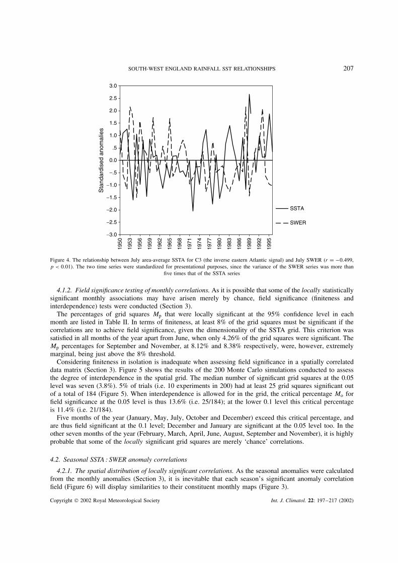
Figure 4. The relationship between July area-average SSTA for C3 (the inverse eastern Atlantic signal) and July SWER (r = −0.499,p < 0.01). The two time series were standardized for presentational purposes, since the variance of the SWER series was more than

five times that of the SSTA series

4.1.2. Field significance testing of monthly correlations. As it is possible that some of the locally statisticallysignificant monthly associations may have arisen merely by chance, field significance (finiteness andinterdependence) tests were conducted (Section 3).

The percentages of grid squares Mp that were locally significant at the 95% confidence level in eachmonth are listed in Table II. In terms of finiteness, at least 8% of the grid squares must be significant if thecorrelations are to achieve field significance, given the dimensionality of the SSTA grid. This criterion wassatisfied in all months of the year apart from June, when only 4.26% of the grid squares were significant. TheMp percentages for September and November, at 8.12% and 8.38% respectively, were, however, extremelymarginal, being just above the 8% threshold.

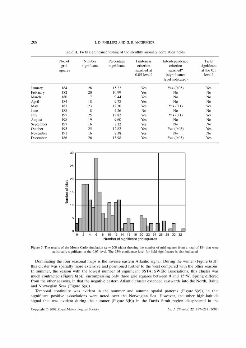
Considering finiteness in isolation is inadequate when assessing field significance in a spatially correlateddata matrix (Section 3). Figure 5 shows the results of the 200 Monte Carlo simulations conducted to assessthe degree of interdependence in the spatial grid. The median number of significant grid squares at the 0.05level was seven (3.8%). 5% of trials (i.e. 10 experiments in 200) had at least 25 grid squares significant outof a total of 184 (Figure 5). When interdependence is allowed for in the grid, the critical percentage Mo forfield significance at the 0.05 level is thus 13.6% (i.e. 25/184); at the lower 0.1 level this critical percentageis 11.4% (i.e. 21/184).

Five months of the year (January, May, July, October and December) exceed this critical percentage, andare thus field significant at the 0.1 level; December and January are significant at the 0.05 level too. In theother seven months of the year (February, March, April, June, August, September and November), it is highlyprobable that some of the locally significant grid squares are merely ‘chance’ correlations.

4.2. Seasonal SSTA : SWER anomaly correlations

4.2.1. The spatial distribution of locally significant correlations. As the seasonal anomalies were calculatedfrom the monthly anomalies (Section 3), it is inevitable that each season’s significant anomaly correlationfield (Figure 6) will display similarities to their constituent monthly maps (Figure 3).



Table II. Field significance testing of the monthly anomaly correlation fields

No. ofgrid

squares

Numbersignificant

Percentagesignificant

Finitenesscriterion

satisfied at0.05 level?

Interdependencecriterionsatisfied?

(significancelevel indicated)

Fieldsignificantat the 0.1

level?

January 184 28 15.22 Yes Yes (0.05) YesFebruary 182 20 10.99 Yes No NoMarch 180 17 9.44 Yes No NoApril 184 18 9.78 Yes No NoMay 187 23 12.30 Yes Yes (0.1) YesJune 188 8 4.26 No No NoJuly 195 25 12.82 Yes Yes (0.1) YesAugust 198 19 9.60 Yes No NoSeptember 197 16 8.12 Yes No NoOctober 195 25 12.82 Yes Yes (0.05) YesNovember 191 16 8.38 Yes No NoDecember 186 26 13.98 Yes Yes (0.05) Yes

Number of significant grid squares32302826242220181614121086420

Num

ber o

f tria

ls

30

25

20

15

10

5

0

Figure 5. The results of the Monte Carlo simulation (n = 200 trials) showing the number of grid squares from a total of 184 that werestatistically significant at the 0.05 level. The 95% confidence level for field significance is also indicated

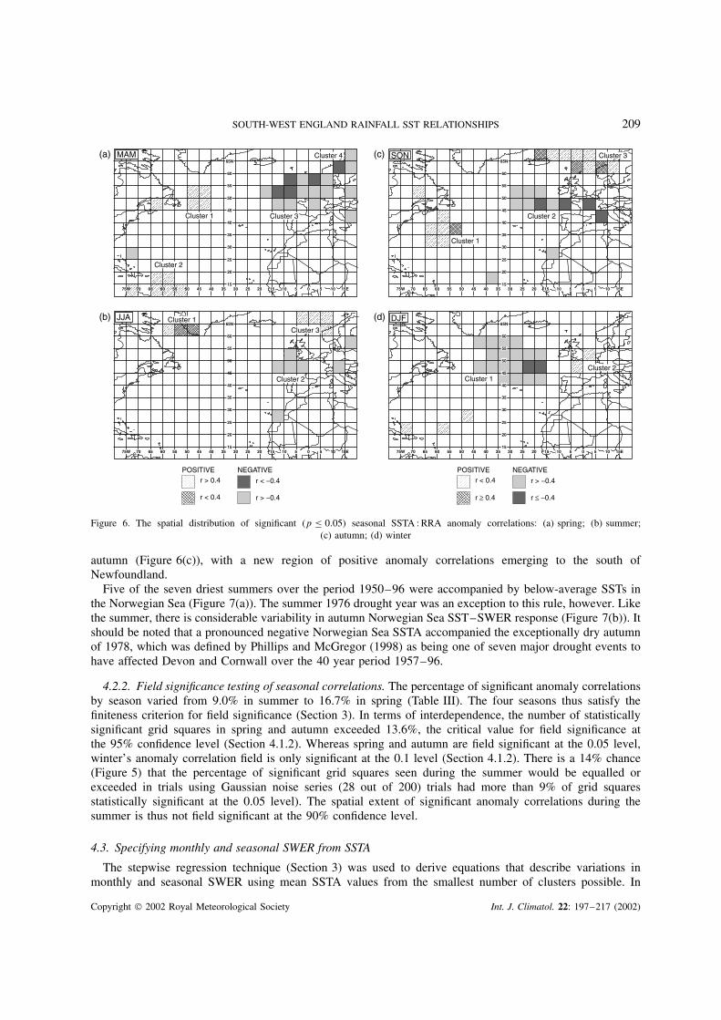
Dominating the four seasonal maps is the inverse eastern Atlantic signal. During the winter (Figure 6(d)),this cluster was spatially more extensive and positioned further to the west compared with the other seasons.In summer, the season with the lowest number of significant SSTA : SWER associations, this cluster wasmuch contracted (Figure 6(b)), encompassing only three grid squares between 0 and 15°W. Spring differedfrom the other seasons, in that the negative eastern Atlantic cluster extended eastwards into the North, Balticand Norwegian Seas (Figure 6(a)).

Temporal continuity was evident in the summer and autumn spatial patterns (Figure 6(c)), in thatsignificant positive associations were noted over the Norwegian Sea. However, the other high-latitudesignal that was evident during the summer (Figure 6(b)) in the Davis Strait region disappeared in the



65N

60

55

50

35

30

25

20

1575W 70 65 60 55 50 45 40 35 30 25 20 10 5 0 5 1015

(a) MAM

Cluster 2

Cluster 1 Cluster 3

Cluster 465N

60

55

50

45

40

35

30

25

20

1575W 70 65 60 55 50 45 40 35 30 25 20 10 5 0 5 10 15E15

(c) SON

Cluster 1

Cluster 2

Cluster 3

65N

60

55

50

45

40

35

30

25

20

1575W 70 65 60 55 50 45 40 35 30 25 20 10 5 0 5 10 15E15

(b) JJA

Cluster 2

Cluster 1

Cluster 365N

60

55

50

45

40

35

30

25

20

1575W 70 65 60 55 50 45 40 35 30 25 20 10 5 0 5 10 15E15

(d) DJF

Cluster 1

Cluster 2

POSITIVE NEGATIVE POSITIVE NEGATIVEr > 0.4

r < 0.4

r < −0.4

r > −0.4

r < 0.4

r ≥ 0.4

r > −0.4

r ≤ −0.4

15E

45

40

Figure 6. The spatial distribution of significant (p ≤ 0.05) seasonal SSTA : RRA anomaly correlations: (a) spring; (b) summer;(c) autumn; (d) winter

autumn (Figure 6(c)), with a new region of positive anomaly correlations emerging to the south ofNewfoundland.

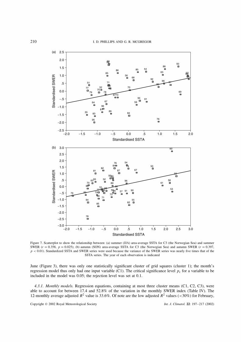
Five of the seven driest summers over the period 1950–96 were accompanied by below-average SSTs inthe Norwegian Sea (Figure 7(a)). The summer 1976 drought year was an exception to this rule, however. Likethe summer, there is considerable variability in autumn Norwegian Sea SST–SWER response (Figure 7(b)). Itshould be noted that a pronounced negative Norwegian Sea SSTA accompanied the exceptionally dry autumnof 1978, which was defined by Phillips and McGregor (1998) as being one of seven major drought events tohave affected Devon and Cornwall over the 40 year period 1957–96.

4.2.2. Field significance testing of seasonal correlations. The percentage of significant anomaly correlationsby season varied from 9.0% in summer to 16.7% in spring (Table III). The four seasons thus satisfy thefiniteness criterion for field significance (Section 3). In terms of interdependence, the number of statisticallysignificant grid squares in spring and autumn exceeded 13.6%, the critical value for field significance atthe 95% confidence level (Section 4.1.2). Whereas spring and autumn are field significant at the 0.05 level,winter’s anomaly correlation field is only significant at the 0.1 level (Section 4.1.2). There is a 14% chance(Figure 5) that the percentage of significant grid squares seen during the summer would be equalled orexceeded in trials using Gaussian noise series (28 out of 200) trials had more than 9% of grid squaresstatistically significant at the 0.05 level). The spatial extent of significant anomaly correlations during thesummer is thus not field significant at the 90% confidence level.

4.3. Specifying monthly and seasonal SWER from SSTA

The stepwise regression technique (Section 3) was used to derive equations that describe variations inmonthly and seasonal SWER using mean SSTA values from the smallest number of clusters possible. In



Standardised SSTA

2.01.51.0.50.0−.5−1.0−1.5−2.0

Sta

ndar

dise

d S

WE

R2.5

2.0

1.5

1.0

.5

0.0

−.5

−1.0

−1.5

−2.0

−2.5

96

95

94

93

9291

89

88

87

86 85

8483

82

81

80

79 78

77

76

75

74

73

71

70

69

68

67

66

65

64

63

61

60

59

58

57

56

55

54

53

52

51

50

Standardised SSTA

3.02.52.01.51.0.50.0−.5−1.0−1.5−2.0

Sta

ndar

dise

d S

WE

R

3.0

2.5

2.0

1.5

1.0

.5

0.0

−.5

−1.0

−1.5

−2.0

−2.5

−3.0

96

95

9493

92

91 90

8988

87

86

85

84

83

8281

80

79

78

77

7674

7372

71

70

69

68

67

6665

64

63

62

61

60

59

58

5756

55

54

53

52

51

50

(a)

(b)

Figure 7. Scatterplot to show the relationship between: (a) summer (JJA) area-average SSTA for C3 (the Norwegian Sea) and summerSWER (r = 0.358, p = 0.025); (b) autumn (SON) area-average SSTA for C3 (the Norwegian Sea) and autumn SWER (r = 0.397,p < 0.01). Standardized SSTA and SWER series were used because the variance of the SWER series was nearly five times that of the

SSTA series. The year of each observation is indicated

June (Figure 3), there was only one statistically significant cluster of grid squares (cluster 1); the month’sregression model thus only had one input variable (C1). The critical significance level pc for a variable to beincluded in the model was 0.05; the rejection level was set at 0.1.

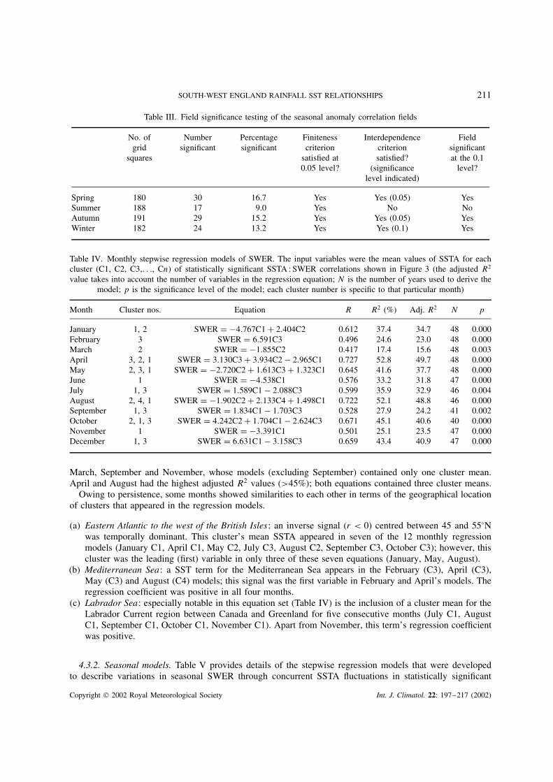
4.3.1. Monthly models. Regression equations, containing at most three cluster means (C1, C2, C3), wereable to account for between 17.4 and 52.8% of the variation in the monthly SWER index (Table IV). The12-monthly average adjusted R2 value is 33.6%. Of note are the low adjusted R2 values (<30%) for February,



Table III. Field significance testing of the seasonal anomaly correlation fields

No. ofgrid

squares

Numbersignificant

Percentagesignificant

Finitenesscriterion

satisfied at0.05 level?

Interdependencecriterionsatisfied?

(significancelevel indicated)

Fieldsignificantat the 0.1

level?

Spring 180 30 16.7 Yes Yes (0.05) YesSummer 188 17 9.0 Yes No NoAutumn 191 29 15.2 Yes Yes (0.05) YesWinter 182 24 13.2 Yes Yes (0.1) Yes

Table IV. Monthly stepwise regression models of SWER. The input variables were the mean values of SSTA for eachcluster (C1, C2, C3,. . ., Cn) of statistically significant SSTA : SWER correlations shown in Figure 3 (the adjusted R2

value takes into account the number of variables in the regression equation; N is the number of years used to derive themodel; p is the significance level of the model; each cluster number is specific to that particular month)

Month Cluster nos. Equation R R2 (%) Adj. R2 N p

January 1, 2 SWER = −4.767C1 + 2.404C2 0.612 37.4 34.7 48 0.000February 3 SWER = 6.591C3 0.496 24.6 23.0 48 0.000March 2 SWER = −1.855C2 0.417 17.4 15.6 48 0.003April 3, 2, 1 SWER = 3.130C3 + 3.934C2 − 2.965C1 0.727 52.8 49.7 48 0.000May 2, 3, 1 SWER = −2.720C2 + 1.613C3 + 1.323C1 0.645 41.6 37.7 48 0.000June 1 SWER = −4.538C1 0.576 33.2 31.8 47 0.000July 1, 3 SWER = 1.589C1 − 2.088C3 0.599 35.9 32.9 46 0.004August 2, 4, 1 SWER = −1.902C2 + 2.133C4 + 1.498C1 0.722 52.1 48.8 46 0.000September 1, 3 SWER = 1.834C1 − 1.703C3 0.528 27.9 24.2 41 0.002October 2, 1, 3 SWER = 4.242C2 + 1.704C1 − 2.624C3 0.671 45.1 40.6 40 0.000November 1 SWER = −3.391C1 0.501 25.1 23.5 47 0.000December 1, 3 SWER = 6.631C1 − 3.158C3 0.659 43.4 40.9 47 0.000

March, September and November, whose models (excluding September) contained only one cluster mean.April and August had the highest adjusted R2 values (>45%); both equations contained three cluster means.

Owing to persistence, some months showed similarities to each other in terms of the geographical locationof clusters that appeared in the regression models.

(a) Eastern Atlantic to the west of the British Isles: an inverse signal (r < 0) centred between 45 and 55°Nwas temporally dominant. This cluster’s mean SSTA appeared in seven of the 12 monthly regressionmodels (January C1, April C1, May C2, July C3, August C2, September C3, October C3); however, thiscluster was the leading (first) variable in only three of these seven equations (January, May, August).

(b) Mediterranean Sea: a SST term for the Mediterranean Sea appears in the February (C3), April (C3),May (C3) and August (C4) models; this signal was the first variable in February and April’s models. Theregression coefficient was positive in all four months.

(c) Labrador Sea: especially notable in this equation set (Table IV) is the inclusion of a cluster mean for theLabrador Current region between Canada and Greenland for five consecutive months (July C1, AugustC1, September C1, October C1, November C1). Apart from November, this term’s regression coefficientwas positive.

4.3.2. Seasonal models. Table V provides details of the stepwise regression models that were developedto describe variations in seasonal SWER through concurrent SSTA fluctuations in statistically significant



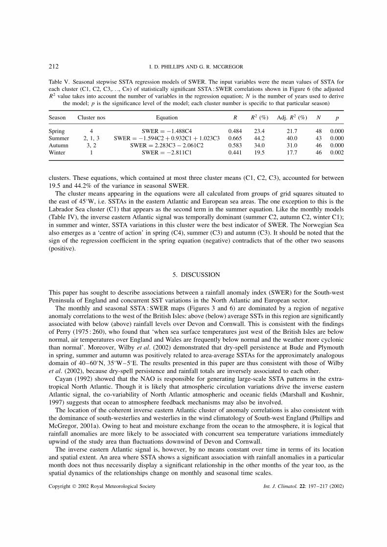
Table V. Seasonal stepwise SSTA regression models of SWER. The input variables were the mean values of SSTA foreach cluster (C1, C2, C3,. . ., Cn) of statistically significant SSTA : SWER correlations shown in Figure 6 (the adjustedR2 value takes into account the number of variables in the regression equation; N is the number of years used to derive

the model; p is the significance level of the model; each cluster number is specific to that particular season)

Season Cluster nos Equation R R2 (%) Adj. R2 (%) N p

Spring 4 SWER = −1.488C4 0.484 23.4 21.7 48 0.000Summer 2, 1, 3 SWER = −1.594C2 + 0.932C1 + 1.023C3 0.665 44.2 40.0 43 0.000Autumn 3, 2 SWER = 2.283C3 − 2.061C2 0.583 34.0 31.0 46 0.000Winter 1 SWER = −2.811C1 0.441 19.5 17.7 46 0.002

clusters. These equations, which contained at most three cluster means (C1, C2, C3), accounted for between19.5 and 44.2% of the variance in seasonal SWER.

The cluster means appearing in the equations were all calculated from groups of grid squares situated tothe east of 45°W, i.e. SSTAs in the eastern Atlantic and European sea areas. The one exception to this is theLabrador Sea cluster (C1) that appears as the second term in the summer equation. Like the monthly models(Table IV), the inverse eastern Atlantic signal was temporally dominant (summer C2, autumn C2, winter C1);in summer and winter, SSTA variations in this cluster were the best indicator of SWER. The Norwegian Seaalso emerges as a ‘centre of action’ in spring (C4), summer (C3) and autumn (C3). It should be noted that thesign of the regression coefficient in the spring equation (negative) contradicts that of the other two seasons(positive).

5. DISCUSSION

This paper has sought to describe associations between a rainfall anomaly index (SWER) for the South-westPeninsula of England and concurrent SST variations in the North Atlantic and European sector.

The monthly and seasonal SSTA : SWER maps (Figures 3 and 6) are dominated by a region of negativeanomaly correlations to the west of the British Isles: above (below) average SSTs in this region are significantlyassociated with below (above) rainfall levels over Devon and Cornwall. This is consistent with the findingsof Perry (1975 : 260), who found that ‘when sea surface temperatures just west of the British Isles are belownormal, air temperatures over England and Wales are frequently below normal and the weather more cyclonicthan normal’. Moreover, Wilby et al. (2002) demonstrated that dry-spell persistence at Bude and Plymouthin spring, summer and autumn was positively related to area-average SSTAs for the approximately analogousdomain of 40–60°N, 35°W–5°E. The results presented in this paper are thus consistent with those of Wilbyet al. (2002), because dry-spell persistence and rainfall totals are inversely associated to each other.

Cayan (1992) showed that the NAO is responsible for generating large-scale SSTA patterns in the extra-tropical North Atlantic. Though it is likely that atmospheric circulation variations drive the inverse easternAtlantic signal, the co-variability of North Atlantic atmospheric and oceanic fields (Marshall and Kushnir,1997) suggests that ocean to atmosphere feedback mechanisms may also be involved.

The location of the coherent inverse eastern Atlantic cluster of anomaly correlations is also consistent withthe dominance of south-westerlies and westerlies in the wind climatology of South-west England (Phillips andMcGregor, 2001a). Owing to heat and moisture exchange from the ocean to the atmosphere, it is logical thatrainfall anomalies are more likely to be associated with concurrent sea temperature variations immediatelyupwind of the study area than fluctuations downwind of Devon and Cornwall.

The inverse eastern Atlantic signal is, however, by no means constant over time in terms of its locationand spatial extent. An area where SSTA shows a significant association with rainfall anomalies in a particularmonth does not thus necessarily display a significant relationship in the other months of the year too, as thespatial dynamics of the relationships change on monthly and seasonal time scales.



Of particular note is the contraction of the statistically significant area from January through to March. InJanuary, a large expanse of ocean to the west of 5°W (covering 20 grid squares) that extends from south-westGreenland to north-west Spain showed significant associations with SWER. By February, this region hadcontracted to ten grid squares, being markedly reduced to only four squares in the western approaches of theBritish Isles in March and remaining spatially constricted in April and May too. Accompanying this trend,the spatially dominant cluster in March was positioned to the east of the British Isles in the North, Norwegianand Baltic Seas, rather than in the eastern Atlantic to the west of Britain. An inverse signal was evidentover the North Sea in May too. This is consistent with the findings of Van Oldenborgh et al. (2000). Theyconstructed a spring precipitation index for Europe centred on 50°N and found that high precipitation wasconcurrently associated with colder water in the north-east Atlantic sector.

The spatial contraction of the region of significant anomaly correlations to the west of the British Islesin spring may reflect the decline in the frequency of westerly winds over Britain at this time of year.Consequently, winds from the northerly and easterly quadrants are more frequent during spring months(Lamb, 1950, 1972). For instance, on 22.71% of spring days (MAM) during the period 1950–97 the winddirection over the British Isles was in the northerly quadrant (Jenkinson and Collison, 1977). This is thehighest frequency of the four seasons and compares with a frequency of only 14.84% experienced during thewinter months (DJF) over this 48 year period. The weakness of this argument for explaining March’s anomalycorrelation field is the absence of significant anomaly correlations to the north and east of Britain in April(Figure 3(d)), a month that is also typically characterized by high frequencies of northerly and easterly winds.

Though the inverse eastern Atlantic cluster was temporally dominant, significant anomaly correlationsin other regions were confined to particular months or seasons. The positive eastern Mediterranean clusterprovides one example of this, being confined to February, April and May. The temporal confinement of theMediterranean signal may be a product of a teleconnection between the El Nino Southern Oscillation (ENSO)phenomenon and European climate variability that results in a subtle movement of the North Atlantic stormtrack.

Studies (e.g. Halpert and Ropelewski, 1992; Van Oldenborgh et al., 2000) have shown that the strongestENSO to European climate associations generally occur in late winter and during the spring. Fraedrich andMuller (1992) found that Western Europe has a greater tendency to be warmer and wetter following an El Ninoevent, as the European storm track takes a more southerly latitude. Laita and Grimalt (1997) also found thatthe most coherent ENSO to pressure anomaly signal over the western Mediterranean was restricted to Marchand April. More recently, the modelling study of Sutton et al. (2000) has revealed that SSTAs generated as aresult of Pacific ENSO events assumed their greatest importance in accounting for the climate variability ofthe tropical Atlantic sector in winter and spring.

The weakness of the ENSO argument for explaining study results is the absence of statistically significantrelationships in the Mediterranean Sea during March. This may reflect not only the weakness of theENSO–European climate teleconnection (correlations rarely exceed 0.4), but also its variability over time.For example, in a study linking ENSO to precipitation over the Iberian Peninsula, Rocha (1999 : 889) notedthat ‘when the ENSO–rainfall association is analysed over a 20-year moving window from 1900 to 1996,it becomes clear it has changed substantially over time’. This partially reflects the fact that seasonal todecadal atmospheric variability in the North Atlantic is not dominated by any single mode, but by ‘multiplecompeting influences of comparable importance’ (Sutton et al., 2000 : 3261) that often arise from localprocesses.

Variations in the Mediterranean climate have also been linked to the NAO (Wanner et al., 1995), animportant source of British climate variability too. Given that SSTs are conditioned by atmospheric processvariations such as the NAO (Marshall and Kushnir, 1997), it is thus perhaps unsurprising that MediterraneanSSTAs should also be linked to rainfall anomalies over South-west England and UK climate variables moregenerally. For instance, Colman (1997) described an SST wave teleconnection in the eastern Mediterraneandownstream of the North Atlantic SST pattern that he used to predict summer CET.

SST ‘centres of action’ emerged at high latitudes during the summer and early autumn. In particular, SWERwas positively related to sea temperatures to the south of Greenland from May to August. In their study,Colman and Davey (1999) found an inverse relationship between SSTA in this area and the concurrent value



of July–August CET. This is consistent with the positive SSTA : SWER correlations presented in this paper,because summer rainfall totals over England and Wales are inversely related to CET (Colman, 1997 : 1299).Positive (negative) SSTAs to the south and west of Greenland during July and August are thus more likelyto result in above (below) average rainfall totals over South-west England during these two months and beaccompanied by lower (higher) CETs.

Positive anomaly correlations south of Greenland may be related to the flow around a deeper than averageIcelandic low (Colman, 1997) that results in westerly wind anomalies across the UK, and hence above averagerainfall over the South-west Peninsula. Such a pattern is evident during the positive phase of the NAO (Lamband Peppler, 1987). Below-average sea temperatures in the vicinity of Greenland may be related to a shallowerIcelandic low and northerly and easterly wind anomalies across Britain, thus leading to negative precipitationanomalies over Devon and Cornwall.

Occurring in five of the 12 monthly regression equations (Section 4.3), a further high-latitude ‘centreof action’ is the Davis Strait between Canada and Greenland. Rodionov and Martin (1999) also identifiedthis north-western Atlantic region in the vicinity of the Labrador Current as being important for feedbackmechanisms between ocean and atmosphere. Semenyuk (1984) described how negative surface air temperatureanomalies in this region are associated with the positive phase of the NAO when the Icelandic low is deeperthan normal. This phase of the NAO is also characterized by the intensification of the Gulf Stream andLabrador Current. Thermal contrasts in the oceanic polar frontal zone are thus sharpened, with enhancedSST gradients promoting cyclonic activity along the front and leading to a deeper than normal Icelandic low.Consequently, this encourages further advection of cold air masses into the north-western Atlantic, and hencemaintains the negative temperature anomalies in this region.

The areal extent of significant SSTA : SWER correlations varies seasonally. Whereas the anomaly correlationpatterns of spring, autumn and winter achieved field significance at the 0.1 level, the percentage of significantgrid squares seen during the summer failed (9.0%) to do so. Likewise, the monthly fields for June andAugust did not satisfy the field significance criteria. This suggests that rainfall anomalies during the summer,when the atmosphere is dynamically less active, are more a function of smaller-scale physical processesthan the synchronous SSTA forcing pattern. Phillips and McGregor (2001b) also found this to be truewhen they replaced sea temperature with monthly zonal water vapour flux anomalies from a selection ofWestern European radiosonde stations in a multiple linear-regression model of SWER. Phillips (2000), inaddition, found that daily rainfall totals over Devon and Cornwall were less dependent on pressure andwesterly wind force variations over the British Isles during the summer when compared with the otherseasons.

Of interest is the anomalously low number of significant anomaly correlations seen in June. This may reflectthe rapid warming of the ocean surface during this month, which may act to conceal any SSTA : SWERrelationships present. Similarly, this might be true of September, a month of transition from summer toautumn, which recorded the second lowest percentage of significant anomaly correlations of the 12 months(Table II).

In general, the regions of significant seasonal anomaly correlations were spatially more coherent andextensive when compared with the constituent monthly maps. This was demonstrated by the fact that onlyfive (January, March, July, October and December) months satisfied the finiteness and interdependence criteriafor field significance at the 0.1 level. Some of the locally significant anomaly correlations that appear in theother seven months, especially squares that occur in isolation, almost certainly represent ‘chance’ correlations.Greater spatial coherence in SSTA : SWER patterns at the seasonal time scale may reflect the slow evolutionof SSTA and the higher degree of noise, and thus internal variability, that is present in the monthly climatesystem.

This paper has demonstrated that statistically significant associations exist between South-west Englandrainfall and concurrent North Atlantic and European sea temperature variations. In spite of this, the percentageof the variance accounted for by SSTA is comparatively low (Tables IV and V) when compared with variablessuch as pressure, vorticity, wind flow components and water vapour flux anomalies. The percentage of variancethat is explained by SSTA in this study is largely consistent with previous research. Examples include theresults of Colman (1997), who found that statistically significant concurrent correlations between July–August



CET and eastern North Atlantic SST did not exceed 0.4. The correlation coefficients reported by Wilby (1998)between daily rainfall characteristics at two English stations and concurrent area-average North Atlantic SSTA(40–60°N, 35°W–5°E) also did not reach the 0.5 level.

Whereas SSTAs evolve slowly and impart a discrete bias on the current, and indeed the future (Pengand Mysak, 1993; Palmer, 1995), atmospheric circulation, fluctuations in atmospheric variables are translatedalmost instantaneously over the synoptic time scale into a surface rainfall anomaly response. For instance,Phillips and McGregor (2001b) found that 69.0% of the variation in monthly SWER could be explainedstatistically by a six-variable model containing water vapour flux anomalies drawn from five Western Europeanradiosonde stations.

6. CONCLUSION

In this study, the nature of concurrent associations between North Atlantic and European SSTA and a regionalrainfall anomaly index for South-west England (SWER) at the monthly and seasonal time scales has beenexplored.

Study results have revealed that SSTA : SWER associations demonstrate variability in their strength bothover space and time. At the two time scales, the most temporally consistent SSTA signal in the SWER seriesoriginates in an area to the west of the British Isles, where depressed (elevated) SSTs are associated withabove (below) average rainfall over South-west England. However, the spatial extent of this teleconnectiondiminishes during the late winter and spring, a trend most likely related to the decline in the frequency ofwesterly winds, and thus atmospheric water vapour flux, from the North Atlantic over the study area at thistime of the year.

This paper has also revealed possible associations between South-west England rainfall and SSTs in theMediterranean for the late winter and spring months. However, the extent to which these reflect an ENSOinfluence is uncertain, as a plausible physical mechanism that accounts for the propagation of ocean-relatedatmospheric circulation, and thus rainfall anomalies, over such large distances to South-west England appearsnot to exist. For the summer and early autumn months, ocean regions to the south and west of Greenlandappear to be important, such that positive (negative) SSTAs are associated with above (below) average rainfalltotals over the study area. It would appear that westerly wind anomalies associated with a deeper than averageIcelandic low, positive SSTAs and a strongly positive phase of the NAO form the atmospheric bridge for thisteleconnection.

Application of field significance tests has revealed that associations between SSTAs and SWER arestatistically more robust at the seasonal than the monthly time scale. Furthermore, the oceanic centres ofaction associated with seasonal SSTA : SWER associations are spatially more coherent and extensive thantheir monthly counterparts, apart from in summer. Field significance tests also point to the possibility thatmany of the SST–rainfall associations reported in the literature for the wider study area may be due topure chance. The lack of significant SSTA : SWER associations for summer may reflect the predominance ofmesoscale convective processes for rainfall production and delivery for the study area during this season. Thiscontrasts with the large-scale advection of moisture from the North Atlantic in strong westerly flows duringthe winter and autumn, and hence the importance of North Atlantic SSTAs. As an extension of this work,running means of SSTA and SWER could be analysed at the two- and three-monthly time scales to discoverif the anomaly correlation maps presented in this paper have failed to detect any SSTA : SWER signals.

Although North Atlantic SSTA–South-west England rainfall associations have been demonstrated, theexplanatory power of SSTA-forced statistical models of SWER appears to be weak when compared withatmosphere-only statistical models. Despite this, the regression equations presented in this paper, whichspecify rainfall over Devon and Cornwall as a product of SSTAs, may form the basis for the developmentof empirical models for the long-range prediction of South-west England rainfall anomalies. These wouldnecessarily require validation with an independent data set and application using predicted SST anomaliesfrom coupled or atmosphere- or ocean-only GCMs. Alternatively, a study of lagged correlations betweenSSTAs and SWER could be used as the basis for developing long-range forecasting models to predict rainfallover South-west England.



ACKNOWLEDGEMENTS

Thanks go to South West Water for supplying us with the rainfall data and to the Hadley Centre (UKMO)for the SST data set. We would also like to acknowledge Kevin Burkhill and Anne Ankcorn of the DrawingOffice, School of Geography and Environmental Sciences, University of Birmingham, for their excellentcartographic work. Thanks also go to Dr Xiaoming Cai, School of Geography, for computing assistance. Theconstructive comments of the two referees are also acknowledged.

REFERENCES

Barnston AG. 1994. Linear statistical short-term climate predictive skill in the Northern Hemisphere. Journal of Climate 7: 1513–1564.Barnston AG, Smith TM. 1996. Specification and prediction of global surface temperature and precipitation. Journal of Climate 9:

2660–2697.Cayan DR. 1992. Latent and sensible heat flux anomalies over the northern oceans: the connection to monthly atmospheric circulation.

Journal of Climate 5: 354–369.Colman AW. 1997. Prediction of summer central England temperature from preceding North Atlantic winter sea surface temperature.

International Journal of Climatology 17: 1285–1300.Colman AW, Davey M. 1999. Prediction of summer temperature, rainfall and pressure in Europe from preceding winter North Atlantic

Ocean temperature. International Journal of Climatology 19: 513–536.Doornkamp JC, Gregory KJ, Burn AS. 1980. Atlas of the Drought in Britain, 1975–76. Institute of British Geographers: 86 pp.Douglas CKM. 1960. Some features of local weather in SE Devon. Weather 15: 14–18.Ebdon D. 1985. Statistics in Geography. Blackwell: 232 pp.Fraedrich K, Muller K. 1992. Climate anomalies in Europe associated with ENSO extremes. International Journal of Climatology 12:

25–31.Halpert MS, Ropelewski CF. 1992. Surface temperature patterns associated with the Southern Oscillation. Journal of Climate 5:

577–593.Hurrell JW. 1995. Decadal trends in the North Atlantic oscillation, regional temperatures and precipitation. Science 269: 676–679.Jenkinson AF, Collison FP. 1977. An initial climatology of gales over the North Sea. Synoptic Climatology Branch Memorandum

No. 62. Meteorological Office: Bracknell.Johansson A, Barnston A, Saha S, Van den Dool H. 1998. On the level and origin of seasonal forecast skill in Europe. Journal of the

Atmospheric Sciences 55: 103–127.Jones PD, Lister DH. 1998. Riverflow reconstructions for 15 catchments over England and Wales and an assessment of hydrologic

drought since 1865. International Journal of Climatology 18: 999–1013.Kilsby CG, Cowpertwait PSP, O’Connell PE, Jones PD. 1998. Predicting rainfall statistics in England and Wales using atmospheric

circulation variables. International Journal of Climatology 18: 523–539.Laita M, Grimalt M. 1997. Vorticity and pressure anomalies in the Western Mediterranean during El Nino/Southern Oscillation extremes.

International Journal of Climatology 17: 475–482.Lamb HH. 1950. Types and spells of weather around the year in the British Isles: annual trends, seasonal structure of the year,

singularities. Quarterly Journal of the Royal Meteorological Society 76: 393–438.Lamb HH. 1972. British Isles weather types and a register of the daily sequence of circulation patterns, 1861–1971. Geophysical

Memoir, 116. HMSO. London, 85 pp.Lamb PJ, Peppler RA. 1987. North Atlantic Oscillation: concepts and an application. Bulletin of the American Meteorological Society

68: 1218–1225.Livezey RE, Chen WY. 1983. Statistical field significance and its determination by Monte Carlo Techniques. Monthly Weather Review

111: 46–59.Marshall J, Kushnir Y. 1997. A ‘white paper’ on Atlantic climate variability. url: http://geoid.mit.edu/ACCP/avehtml.html. Massachusetts

Institute of Technology and the Lamont–Doherty Earth Observatory of Columbia University. First published in April 1997. Accessedon 30th June, 1999.

McIlveen R. 1992. Fundamentals of Weather and Climate. Chapman and Hall: London; 497 pp.Mo KC, Paegle JN. 2000. Influence of sea surface temperature anomalies on the precipitation regimes over the southwest United States.

Journal of Climate 13: 3588–3598.Murray R, Ratcliffe RAS. 1969. The summer weather of 1968: related atmospheric circulation and sea temperature patterns.

Meteorological Magazine 98: 201–219.Office for National Statistics (ONS). 1999. Regional Trends 34. HMSO: London.Palmer TN. 1993. Extended-range prediction and the Lorenz model. Bulletin of the American Meteorological Society 74: 49–65.Palmer TN. 1995. The influence of north-west Atlantic sea surface temperature: an unplanned experiment. Weather 50: 413–419.Parker DE, Folland CK, Bevan A, Ward MN, Jackson M, Maskell K. 1995. Marine surface data for analyses of climatic fluctuations

on inter-annual to century time-scales, In Climate Variability on Decade to Century Time-scales. US National Academy of Science:Washington, DC.

Peng S, Mysak LA. 1993. A teleconnection study of inter-annual sea surface temperature fluctuations in the northern North Atlanticand precipitation and runoff over western Siberia. Journal of Climate 6: 876–885.

Perry AH. 1975. Eastern North Atlantic sea-surface temperature anomalies and concurrent temperature and weather patterns over theBritish Isles. Weather 30: 258–261.

Perry AH. 1997. South-west England and the Channel Islands, In Regional Climates of the British Isles, Wheeler D, Mayes J (eds).Routledge: London; 47–66.



Phillips ID. 2000. The occurrence, dynamical structure and prediction of drought events over Devon and Cornwall over a forty yearperiod. Unpublished PhD Thesis, School of Geography and Environmental Sciences, University of Birmingham, UK.

Phillips ID, McGregor GR. 1998. The utility of a drought index for assessing the drought hazard in Devon and Cornwall, South WestEngland. Meteorological Applications 5: 359–372.

Phillips ID, McGregor GR. 2001a. The relationship between synoptic scale airflow direction and daily rainfall: a methodology appliedto Devon and Cornwall, South West England. Theoretical and Applied Climatology 69: 179–198.

Phillips ID, McGregor GR. 2001b. Western European water vapour flux–South West England rainfall associations. Journal ofHydrometeorology 2: 505–524.

Ratcliffe RAS. 1977. The wet spell of September–October 1976. Weather 32: 36–37.Ratcliffe RAS, Murray R. 1970. New lag associations between North Atlantic sea temperature and European pressure applied to

long-range weather forecasting. Quarterly Journal of the Royal Meteorological Society 96: 226–246.Rocha A. 1999. Low-frequency variability of seasonal rainfall over the Iberian Peninsula and ENSO. International Journal of Climatology

19: 889–901.Rodionov SN, Martin JH. 1999. An expert system-based approach to prediction of year-to-year climate variations in the North Atlantic

region. International Journal of Climatology 19: 951–974.Semenyuk EA. 1984. The role of thermal conditions of sea surface in formation of persistence of temperature anomaly field. In

Trudy Vsesoyuznogo Nauchno-Issledovatel’skogo Instituta Gidrometeorologicheskoi Informatsii–Mirovoi Tsentr Dannyh (VNI-IGMI-MCD) (Proceedings of the All-Union Research Institute of Hydrometeorological Information–World Data Center), vol. 117; 5–15(in Russian).

Sims FP. 1960. The annual and diurnal variation of shower frequency at St. Eval and St. Mawgan. Meteorological Magazine 89:293–297.

Sutton RT, Jewson SP, Rowell DP. 2000. The elements of climate variability in the Tropical Atlantic region. Journal of Climate 13:3261–3284.

Thacker WC, Lewandowicz R. 1997. Partitioning the North Atlantic into regions of similar seasonal sea-surface temperature anomalies.International Journal of Climatology 17: 3–23.

Van Oldenborgh GJ, Burgers G, Tank AK. 2000. On the El Nino teleconnection to spring precipitation in Europe. International Journalof Climatology 20: 565–574.

Wanner H, Pfister C, Brazdil R, Frich P, Frydendahl K, Jonsson T, Kington J, Lamb HH, Rosenorn S, Wishman E. 1995. WintertimeEuropean circulation patterns during the Late Maunder Minimum cooling period (1675–1704). Theoretical and Applied Climatology51: 167–175.

Wilby RL. 1998. Statistical downscaling of daily precipitation using daily airflow and seasonal teleconnection indices. Climate Research10: 163–178.

Wilby RL, Conway D, Jones PD. In press. Prospects for downscaling seasonal precipitation variability using conditioned weathergenerator parameters. Hydrological Processes.

Wilks DS. 1995. Statistical Methods in the Atmospheric Sciences. Academic Press: San Diego; 467 pp.


The relationship between monthly and seasonal South-west England rainfall anomalies and concurrent...

Documents

Transcript of The relationship between monthly and seasonal South-west England rainfall anomalies and concurrent...