This article appeared in a journal published by Elsevier. The attachedcopy is furnished to the author for internal non-commercial researchand education use, including for instruction at the authors institution

and sharing with colleagues.

Other uses, including reproduction and distribution, or selling orlicensing copies, or posting to personal, institutional or third party

websites are prohibited.

In most cases authors are permitted to post their version of thearticle (e.g. in Word or Tex form) to their personal website orinstitutional repository. Authors requiring further information

regarding Elsevier’s archiving and manuscript policies areencouraged to visit:

http://www.elsevier.com/copyright

Author's personal copy

e c o l o g i c a l m o d e l l i n g 2 2 0 ( 2 0 0 9 ) 533–544

avai lab le at www.sc iencedi rec t .com

journa l homepage: www.e lsev ier .com/ locate /eco lmodel

The puzzle of North America’s Late Pleistocene megafaunalextinction patterns: Test of new explanation yieldsunexpected results

Jeffrey V. Yulea,∗, Christopher X.J. Jensenb,c, Aby Josephc, Jimmie Gooded

a School of Biological Sciences, P.O. Box 3179, Louisiana Tech University, Ruston, LA 71272, USAb Department of Mathematics and Science, Pratt Institute, 200 Willoughby Avenue, Brooklyn, NY 11205, USAc Department of Ecology and Evolution, SUNY Stony Brook, Stony Brook, NY 11794, USAd Department of Mathematics, Louisiana Tech University, Ruston, LA 71272, USA

a r t i c l e i n f o

Article history:

Received 18 July 2008

Received in revised form

20 October 2008

Accepted 31 October 2008

Published on line 6 January 2009

Keywords:

Pleistocene extinctions

Megafauna

Overkill

Allometric constraint

Functional response

Model assessment

Model design methodology

Parameterization

a b s t r a c t

Although Late Pleistocene extinctions disproportionately affected larger mammalian

species, numerous smaller species were also lost. To date, no satisfactory explanation has

been presented to account for this pattern. Beginning with the assumption that human pre-

dation caused the extinctions, we offer and test the first such explanatory hypothesis, which

is predicated on considering more realistic functional response forms (i.e., those that allow

for predator interference or prey sharing). We then test the hypothesis via a one-predator,

six-prey ecological model that maintains transparency, minimalism of design, and maximal

constraint of parameters. Results indicate that altering assumptions about one cornerstone

of ecological modeling (i.e., functional response) fails to produce qualitative differences in

survival–extinction outcomes—even in conjunction with a wide range of capture efficiency

permutations. This unexpected finding suggests that no reasonable form of predation alone

is capable of producing the survival–extinction pattern observed. We conclude that the mat-

ter of causation and the conclusions of previous Late Pleistocene extinction models remain

far less certain than many have assumed.

© 2008 Elsevier B.V. All rights reserved.

1. Introduction

Late Pleistocene megafaunal extinctions occurred globallyover a period of roughly 50,000 years, most severely affect-ing large (≥44 kg body mass) mammals in Australia, Eurasia,and the Americas (Johnson, 2002; Barnosky et al., 2004;Koch and Barnosky, 2006). Polarized debate about the causesof the extinctions dates back to the nineteenth century,centering on anthropogenic effects (especially hunting) andclimate (Grayson, 1984). Mathematical models have been

∗ Corresponding author.E-mail address: jyule@latech.edu (J.V. Yule).

developed since the 1960s that seek to explain the extinctions(Budyko, 1967, 1974), but none have been entirely successfulin explaining observed extinction patterns. Here, we assumethat human hunting caused the extinctions and then go onto develop and test a mathematical conjecture about LatePleistocene megafaunal extinctions that is more accurate inaccounting for the general pattern of extinctions, more trans-parent, and simpler than the best-known recent model (Alroy,2001). Our approach emphasizes the value of minimalist,transparent, open-access modeling efforts.

0304-3800/$ – see front matter © 2008 Elsevier B.V. All rights reserved.doi:10.1016/j.ecolmodel.2008.10.023

Author's personal copy

534 e c o l o g i c a l m o d e l l i n g 2 2 0 ( 2 0 0 9 ) 533–544

2. Refining Late Pleistocene extinctionmodels

Alroy (2001) offers a computer simulation that purportsto demonstrate that human hunting alone adequatelyexplains Late Pleistocene megafaunal extinction patterns.Alroy’s results have sometimes been interpreted (e.g., Koch,2006) as lending strong support to the overkill hypoth-esis (i.e., that extinctions resulted from overhunting byhumans) as first articulated by Martin (1967) and laterrefined and modeled by Mosimann and Martin (1975). Ourresearch indicates that such an interpretation of the model-ing evidence is premature and potentially incorrect. Alroy’s(2001) model performs slightly better than a simplest case“model” that separates North American mammals into twogroups based on mass – with a boundary between 118 kgand 223 kg – and assumes that all species above thisthreshold went extinct while all those below it survived(Fig. 1).

In part, Alroy (2001) assesses his model by comparing itsoutcomes to those of this simple one-line method. Delineat-ing such an extinction boundary on the basis of mass correctlypredicts 30 of 41 (73%) of actual survival–extinction outcomes,while Alroy’s mechanistic model correctly predicts 32 of 41(78%) of outcomes (Alroy, 2001). Alroy’s simulation brings awelcome element of ecological interactivity to Late Pleistoceneextinction modeling, particularly in regard to its linkage

between predator hunting success and predator reproduction.However, because the model simultaneously incorporatesmultiple complicating factors and is not an open accessresource, it remains unclear how the simulation achieves thisslight improvement over a simplest case approach. Part of theimprovement might result from assumptions about the initialabundances of rarer species with limited geographic ranges(i.e., the pronghorns Stockoceros conklingi and Stockoceros onus-rosagris) (J. Alroy, personal communication, 2006). Critiquesof common modeling approaches (e.g., Ginzburg and Jensen,2004) suggest that part of the improvement might also resultfrom over parameterization (i.e., “fitting” a model to a particu-lar data set by adding numerous unconstrained parameters).Such a suggestion is partially borne out by the depiction of thenumerous parameter combinations that were run in achievinga best match to historical data (Alroy, 2001).

Many different models can explain a given situation (e.g.,Brook and Bowman, 2004; Ginzburg and Jensen, 2004), butthe consequences of this fact have been overlooked in therecent debate about Late Pleistocene extinctions. In theabsence of transparency and simplicity, competing mod-els have very limited means of distinguishing themselves.Given enough freedom to add parameters or assume partic-ular values for critical parameters, a competent modeler canachieve a desired result, whether that is general extinctionor survival of megafauna facing human hunting pressure.But a simple model that performs well from the outsetis generally a more significant achievement than a highly

Fig. 1 – Simple one-line method of predicting Late Pleistocene mammalian extinctions in North America. Alroy (2001)achieves two additional correct outcome matches than this simplest-case method but does so at the expense ofconsiderable complexity and lost transparency. Data and method from Alroy (2001).

Author's personal copy

e c o l o g i c a l m o d e l l i n g 2 2 0 ( 2 0 0 9 ) 533–544 535

parameterized model that reaches some desired goal afterconsiderable trial and error in fitting to data (Ginzburg andJensen, 2004).

3. Berezovskaya–Karev–Arditi (BKA) spaceand the two-line method

Common sense suggests that larger species would be atgreater risk of extinction, because greater mass correlates withnumerous traits that increase extinction risk (e.g., decreasedmaximal rate of population increase, rmax, increased homerange size, reduced population size) (e.g., Peters, 1983;Johnson, 2002). Amongst the heaviest species (i.e., ≥500 kg),both Alroy’s simulation and the single-line method performvery well. Granted, there are exceptions, but those are to beexpected; mass correlates with many ecologically relevanttraits but not with all of them.

Both the single-line method and the Alroy simulationperform poorly in predicting survival–extinction outcomesamong smaller species (i.e., those weighing ≤55 kg). Althoughcommon sense suggests that smaller species should be atreduced risk of extinction, a cluster of extinctions occurredamongst these species. Intriguingly, however, ratio-dependentfunctional response assumptions predict increased risk ofextinction at higher and lower prey masses with reducedextinction risk at intermediate masses, thus laying thegroundwork for a promising alternative modeling approach.

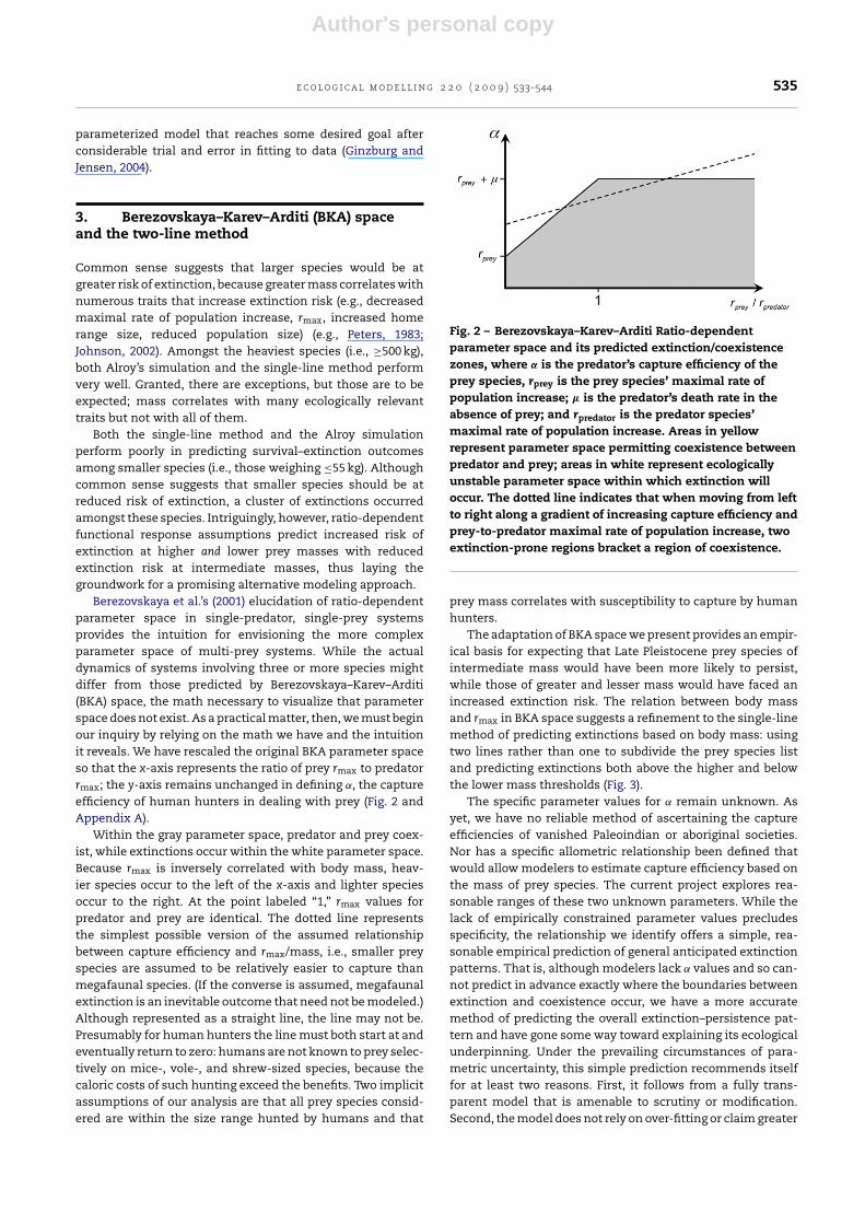
Berezovskaya et al.’s (2001) elucidation of ratio-dependentparameter space in single-predator, single-prey systemsprovides the intuition for envisioning the more complexparameter space of multi-prey systems. While the actualdynamics of systems involving three or more species mightdiffer from those predicted by Berezovskaya–Karev–Arditi(BKA) space, the math necessary to visualize that parameterspace does not exist. As a practical matter, then, we must beginour inquiry by relying on the math we have and the intuitionit reveals. We have rescaled the original BKA parameter spaceso that the x-axis represents the ratio of prey rmax to predatorrmax; the y-axis remains unchanged in defining ˛, the captureefficiency of human hunters in dealing with prey (Fig. 2 andAppendix A).

Within the gray parameter space, predator and prey coex-ist, while extinctions occur within the white parameter space.Because rmax is inversely correlated with body mass, heav-ier species occur to the left of the x-axis and lighter speciesoccur to the right. At the point labeled “1,” rmax values forpredator and prey are identical. The dotted line representsthe simplest possible version of the assumed relationshipbetween capture efficiency and rmax/mass, i.e., smaller preyspecies are assumed to be relatively easier to capture thanmegafaunal species. (If the converse is assumed, megafaunalextinction is an inevitable outcome that need not be modeled.)Although represented as a straight line, the line may not be.Presumably for human hunters the line must both start at andeventually return to zero: humans are not known to prey selec-tively on mice-, vole-, and shrew-sized species, because thecaloric costs of such hunting exceed the benefits. Two implicitassumptions of our analysis are that all prey species consid-ered are within the size range hunted by humans and that

Fig. 2 – Berezovskaya–Karev–Arditi Ratio-dependentparameter space and its predicted extinction/coexistencezones, where ˛ is the predator’s capture efficiency of theprey species, rprey is the prey species’ maximal rate ofpopulation increase; � is the predator’s death rate in theabsence of prey; and rpredator is the predator species’maximal rate of population increase. Areas in yellowrepresent parameter space permitting coexistence betweenpredator and prey; areas in white represent ecologicallyunstable parameter space within which extinction willoccur. The dotted line indicates that when moving from leftto right along a gradient of increasing capture efficiency andprey-to-predator maximal rate of population increase, twoextinction-prone regions bracket a region of coexistence.

prey mass correlates with susceptibility to capture by humanhunters.

The adaptation of BKA space we present provides an empir-ical basis for expecting that Late Pleistocene prey species ofintermediate mass would have been more likely to persist,while those of greater and lesser mass would have faced anincreased extinction risk. The relation between body massand rmax in BKA space suggests a refinement to the single-linemethod of predicting extinctions based on body mass: usingtwo lines rather than one to subdivide the prey species listand predicting extinctions both above the higher and belowthe lower mass thresholds (Fig. 3).

The specific parameter values for ˛ remain unknown. Asyet, we have no reliable method of ascertaining the captureefficiencies of vanished Paleoindian or aboriginal societies.Nor has a specific allometric relationship been defined thatwould allow modelers to estimate capture efficiency based onthe mass of prey species. The current project explores rea-sonable ranges of these two unknown parameters. While thelack of empirically constrained parameter values precludesspecificity, the relationship we identify offers a simple, rea-sonable empirical prediction of general anticipated extinctionpatterns. That is, although modelers lack ˛ values and so can-not predict in advance exactly where the boundaries betweenextinction and coexistence occur, we have a more accuratemethod of predicting the overall extinction–persistence pat-tern and have gone some way toward explaining its ecologicalunderpinning. Under the prevailing circumstances of para-metric uncertainty, this simple prediction recommends itselffor at least two reasons. First, it follows from a fully trans-parent model that is amenable to scrutiny or modification.Second, the model does not rely on over-fitting or claim greater

Author's personal copy

536 e c o l o g i c a l m o d e l l i n g 2 2 0 ( 2 0 0 9 ) 533–544

Fig. 3 – Two-line method of predicting Late Pleistocene mammalian extinctions. This simplified, intuitive approach achievestwo more correct outcome matches than Alroy’s (2001) opaque and much more complex method. Data from Alroy (2001).

precision than prevailing parameteric uncertainty can justify.It is a simpler modeling tool but one that has the potential towork.

4. Methods

To test our hypothesis, we explored the parameter spacedynamics of a multi-prey system. We developed a one-predator, six-prey deterministic numerical simulation modelrelying on ordinary differential equations. The prey growthcomponent generalizes as:

dNi

dt= rmaxi

Ni

(1 − Ni

Ki

)− f (·)iP, (1)

where i = 1, 2, . . ., 6 with i representing the ith prey species, N isthe population size, K is the carrying capacity, f(·)i representsthe functional response form for the predator’s capture of theith prey species, and P is the predator density.

To determine whether functional response choices incor-porating predator interference or prey sharing would pro-vide a better match to observed extinction patterns, wetested the model under three different functional responseassumptions: the Holling Disc Equation (“Type II” PreyDependence, which does not include predator interference),Beddington–DeAngelis (a simple derivative of the Holling DiscEquation incorporating a predator interference parameter,i, which provides a measure of the time spent interacting

with other predators), and Ratio Dependence (which assumescomplete sharing of prey among predators, an assumptionconsistent with a technologically sophisticated, cooperativelyforaging omnivore exploiting available prey) (see Table 1 for asummary comparison of how the current model compares toother major published Late Pleistocene extinction models).

Holling Disc/Type II functional response is represented bythe expression:

f (N)i = aiNi

1 +∑6

i=1aihiNi

, (2)

where a is the predator capture efficiency and h is the han-dling time (i.e., the time between a predator capturing one preyitem and the next). The Beddington–DeAngelis elaboration ofHolling Type II is represented by the expression:

f (N, P)i = aiNi

1 +∑6

i=1aihiNi + iP, (3)

The final functional response form, Ratio Dependence, isrepresented by the expression:

f

(N

P

)i= ˛i(Ni/P)

1 +∑6

i=1˛i(Ni/P), (4)

where ˛ is the predator capture efficiency.

Author's personal copy

e c o l o g i c a l m o d e l l i n g 2 2 0 ( 2 0 0 9 ) 533–544 537Ta

ble

1–

Su

mm

ary

com

par

ison

ofm

ajor

Late

Plei

stoc

ene

exti

nct

ion

mod

els.

Mod

elN

um

ber

ofp

rey

spec

ies

mod

elle

dFo

rmof

mod

elD

ynam

icin

tera

ctio

nin

pre

dat

or–p

rey

dem

ogra

ph

ics?

Fun

ctio

nal

resp

onse

form

Full

and

tran

spar

ent

pre

sen

tati

onof

mod

el

Bu

dyk

o(1

967,

1974

)1

Dif

fere

nti

aleq

uat

ion

No

Un

rela

ted

top

rey

den

sity

Yes

Mos

iman

nan

dM

arti

n(1

975)

1D

iffe

ren

ceeq

uat

ion

No

Un

rela

ted

top

rey

den

sity

No

Wh

itti

ngt

onan

dD

yke

(198

4)1

Dif

fere

nce

equ

atio

nN

oU

nre

late

dto

pre

yd

ensi

tyN

o

Bel

ovsk

y(1

987,

1988

)2

(hu

nte

dfo

od,

gath

ered

food

)D

iffe

ren

ceeq

uat

ion

Yes

Spec

ialc

ase

Yes

Win

terh

ald

eret

al.(

1988

)1

or2

Dif

fere

nce

equ

atio

nY

esSp

ecia

lcas

eN

oW

inte

rhal

der

and

Lu(1

997)

Up

to4

Dif

fere

nce

equ

atio

nY

esSp

ecia

lcas

eN

oC

hoq

uen

otan

dB

owm

an(1

998)

1N

/AN

oH

olli

ng

IIN

oA

lroy

(200

1)42

Dif

fere

nce

equ

atio

nY

esU

niq

ue

form

No

Bro

okan

dB

owm

an(2

002)

1D

iffe

ren

ceeq

uat

ion

No

Hol

lin

gII

IN

oB

rook

and

Bow

man

(200

4)1

Dif

fere

nce

equ

atio

nN

oH

olli

ng

III

No

Yu

leet

al.(

2009

)6

Dif

fere

nti

aleq

uat

ion

Yes

Hol

lin

gII

,B

edd

ingt

on–D

eAn

geli

s,an

dR

atio

Dep

end

ence

Yes

Table 2 – Prey Species Included in Models.

Species Mass (kg) Status

Capromeryx minor (Dimunitive pronghorn) 21 ExtinctPecari tajacu (Collared peccary) 30 SurvivingOdocoileus hemionus (Mule deer) 118 SurvivingEquus conversidens (Mexican horse) 306 ExtinctMegalonyx jeffersonii (Jefferson’s ground sloth) 1320 ExtinctMammuthus columbi (Columbian mammoth) 5827 Extinct

The change in density of human predators is described bythe model’s final equation:

dP

dt=

6∑i=1

eiFRi − 0.067P, (5)

where e is the predator conversion rate of prey to offspring and0.067 is the predator death rate in the absence of prey. Here,the predator growth rate is determined by the summation ofprey offtake minus a death rate in the absence of prey, creatingan explicit link between predator success and reproduction.

The six prey species we consider include both extant andextinct species (Table 2). They were selected both to providea range of size classes and to include species that brackethistorical survival–extinction outcomes that are difficult toexplain solely on the basis of allometric relationships betweenbody mass and rmax (Fig. 1). The species are: Capromeryx minor(21 kg), Pecari tajacu (30 kg), Odocoileus hemionus (118 kg), Equusconversidens (306 kg), Megalonyx jeffersonii (1320 kg), and Mam-muthus columbi (5827 kg).

We constrained all parameters using established allometricrelationships when such relationships were known or by mak-ing explicit assumptions (Table 3). One key allometry remainsundefined: the relationship between prey mass and predatorefficiency in capturing prey. Our secondary goal in construct-ing the model was to explore the unknown allometry forcapture efficiency, which involves two unconstrained param-eters: the capture efficiency constant and capture efficiencyallometric scaling power. While the two varieties of captureefficiency that occur in the functional response forms weexplore are analogous in terms of their biological meaning,they have different units and so are not directly compara-ble. In the Holling II and Beddington–DeAngelis functionalresponses, capture efficiency is denoted by a and is measuredin units of 1/time × individual. Under Ratio Dependence, cap-ture efficiency is denoted by ˛ and is measured in units of1/time. Regardless of units, the postulated allometric rela-tionship between prey body mass, mi, and capture efficiencyare analogous, depending on some capture efficiency power,PowerCE, for both functional response forms and one of twoconstants, Ca and C˛, which differ between the two functionalresponse forms, as follows:

a = CamPowerCEi (6)

˛ = C˛mPowerCEi (7)

Without assuming that Ca = C˛, we explored various estimatesof Ca, C˛, and PowerCE by testing a wide range of parameter

Author's personal copy

538 e c o l o g i c a l m o d e l l i n g 2 2 0 ( 2 0 0 9 ) 533–544

Table 3 – Parameterizations—allometric constraints and assumptions.

Parameter Allometric power assumed Source

rmax (maximal rate of population increase) −0.36 Caughley and Krebs (1983)K (carrying capacity) −0.75 Damuth (1987)e (conversion efficiency) 1 Assumption: all herbivore flesh has equal per kg

nutritional valueh (handling time) 1 Assumption: time to prepare and digest

herbivore flesh is proportional to its massa or ˛ (capture efficiency) Unknown The parameter our model explores

combinations and evaluating the match between simulatedand actual extinction outcomes.

Our approach involved no difficulties for the Holling TypeII and Beddington–DeAngelis models, but one aspect of theratio-dependent model requires clarification in regard to apotential complicating factor. The ratio-dependent functionalresponse contains the rational expression:

˛(N/P)1 + ˛h(N/P)

Because the predator density, P, reaches zero for a varietyof parameterizations, the expression (N/P) becomes meaning-less, causing the numerical simulation algorithm to produceerror messages. We addressed this issue by designing themodel to set functional response to zero when P equals zero.

Simulations were performed using a Mathematica note-book composed of three modules. The first module performsnumerical simulations representing the interaction betweenhuman predators and six prey species. The model requires

nine input parameters that were held constant between allsimulations: initial predator abundance (defined as a densityof 0.1 per km2), predator extinction threshold (defined as adensity of 0.01 per km2), the mass of the each of the six preyspecies, and the number of one-year time steps (500). Theinitial module computes remaining parameters (i.e., carry-ing capacity, rmax, conversion efficiency, handling time) usingestablished allometric relationships or stated assumptions(Table 3).

The output of this model is a set of six lists, each one rep-resenting a time series of abundances for the six prey speciesand the population of human predators. The second moduleanalyzes these lists and looks for extinction events, whichare defined as any prey population that decreases to 5% orless of its carrying capacity. (Human carrying capacity is notdefined a priori but is instead determined by hunting success.)Once an extinction event is discovered, all other abundancesare set to the abundance at the time of the extinctionevent.

Fig. 4 – Model flow chart.

Author's personal copy

e c o l o g i c a l m o d e l l i n g 2 2 0 ( 2 0 0 9 ) 533–544 539

Fig. 5 – Survival–extinction outcomes.

The third module defines parameter space in two dimen-sions: (1) the allometric constant for capture efficiency (Ca

or C˛) and (2) the allometric power for capture efficiency(PowerCE). For each combination of parameters, the moduleperforms a numerical simulation and checks for extinction,reiterating this process until all species are extinct or allremaining species coexist for the full 500-year simulation(Fig. 4). Exploring the two dimensions of the capture efficiencyallometry, this module color-codes each outcome and createsa graphical representation of system stability (Fig. 5).

All simulations were performed using Mathematica version6.0.2.1 and are available on request from the correspondingauthor.

5. Results

Changes in functional response form yielded only minimalqualitative differences in survival–extinction patterns (Fig. 5).Observed differences in the juxtaposition of particular out-comes occurred in only a small portion of the total parameterspace that we have no a priori justification for identifying asbeing particularly biologically relevant. Because we do notknow where reality falls in the parameter space, we have nobasis for suggesting that the particular outcomes associatedwith particular parameter combinations represent or approx-imate actual events.

Survival–extinction outcomes depend on the combinedabsolute magnitudes of hunting pressure (Ca or C˛) and therelative susceptibility of prey species to human hunters,

PowerCE. Total extinction occurs in the top right region ofparameter space, where capture efficiency is highest and preymass has the least influence on how easy a prey item is tocapture. Predator extinction occurs in the bottom left regionof parameter space, where capture efficiency is lowest andthe highest mass prey species are significantly more diffi-cult to capture. Predator–prey coexistence occurs in regionsof intermediate capture efficiency. The transition from coex-istence varies between functional response forms but occursin the general region of PowerCE > −0.35, depending on theoverall intensity of hunting pressure (Ca or C˛). Where Pow-erCE < −0.35, stepwise extinctions eliminate species fromsmallest to largest when hunting pressure is greatest. WherePowerCE > −0.35, stepwise extinctions eliminate species fromlargest to smallest at lower levels of hunting pressure. Increas-ing levels of predator interference lead to increasing systemstability (i.e., a larger region of coexistence). At higher inter-ference levels, the transition that dominates the region ofparameter space explored is the extinction of high mass prey.At lower interference levels, the transition that dominates isthe extinction of low mass prey. We observed no parametercombinations yielding the result predicted by the BKA hypoth-esis.

6. Discussion

The model we present assumes a starting human populationdensity of 0.1 per km2 in North America, depicting a sce-nario in which hunters and prey form a well-mixed system.

Author's personal copy

540 e c o l o g i c a l m o d e l l i n g 2 2 0 ( 2 0 0 9 ) 533–544

Hunters take prey nonselectively on the basis of availability(i.e., more abundant prey are more likely to be encounteredand hunted than rare prey; no prey species are given partic-ular priority). The model then explores extinction dynamicsover a 500-year period of hunting. A spatially explicit modelfollowing the movements of an advancing front of hunters –as per Mosimann and Martin (1975) or Alroy (2001) – mightmore realistically depict some aspects of predator–prey inter-actions. But for present purposes our approach recommendsitself for at least three reasons.

First, our goal was to examine the effects of functionalresponse in the absence of other factors; assuming a well-mixed system achieves that goal. Second, while adding aspatially explicit component to the model might increase ordecrease extinction probabilities, it would probably not affectthe pattern of extinctions, and our goal was to assess pat-terns. Third, given the prevailing uncertainty about the time(s)and route(s) of human entry into North America and grow-ing knowledge of both Paleoindian foraging and the durationof human–megafauna sympatry (e.g., Graf and Schmitt, 2007;Mithen, 2004; Webb, 2006), our starting assumptions may rea-sonably approximate reality. Under the circumstances, then,the current model allows for a preliminary assessment offunctional response’s potential role in clarifying Pleistoceneextinction patterns.

In our simulations, the coexistence transition that occursin the region of PowerCE = −0.35 represents the tipping pointbetween the relative importance of prey rmax and predatorcapture efficiency. When PowerCE < −0.35, larger prey are somuch more difficult to capture than smaller prey that theypersist despite their relatively low rmax values. Conversely,smaller species are eliminated despite their relatively highrmax values because of the extremely high hunting pres-sure they face. When PowerCE > −0.35, larger prey are onlymarginally more difficult to capture than smaller prey, andtheir relatively low rmax values cannot compensate for hunt-ing pressure. Conversely, in this region of parameter space therelatively high rmax values of smaller species are sufficient tocompensate for the reduced hunting pressure they face.

We find no support for the hypothesis that ratio-dependentfunctional response offers a superior explanation for LatePleistocene extinction patterns. All functional response vari-ants demonstrate that the “single line” hypothesis provides areasonable baseline explanation for the extinction of eitherlarger or smaller prey species, depending on the relativemagnitudes of hunting pressure and prey rmax but not simul-taneously in a manner that would provide a closer matchto observed extinction patterns. This negative finding raisesa matter of considerable importance in a broader modelingcontext. Appropriate functional response choice is consideredto be critical for achieving ecologically realistic outcomes inpredator–prey models (e.g., Skalski and Gilliam, 2001; Fenlonand Faddy, 2006). Yet our results indicate a predator–preycontext in which survival–extinction outcomes are relativelyinsensitive to varied functional response choice.

We are left to explain the inability of all models to matchobserved survival–extinction outcomes. If our results are cor-rect, differences in functional response cannot account forthese shortcomings. Our results may represent evidence thatthe functional response predictions of obligate predator–prey

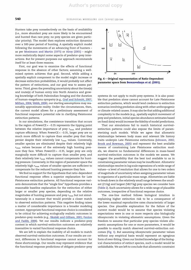
Fig. 6 – Original representation of Ratio-Dependentparameter space from Berezovskaya et al. (2001).

systems do not apply to multi-prey systems. It is also possi-ble that predation alone cannot account for Late Pleistoceneextinction patterns, which would lend credence to extinctionscenarios involving predation along with other anthropogenicor climate-related causes. It may also be that adding additionalcomplexity to the models (e.g., spatially explicit movement ofprey and predators, initial species abundance estimates basedon fossil data) would increase the fidelity of model predictions.

That our simulations fail to match historical survival–extinction patterns could also expose the limits of param-eterizing such models. While we agree that allometricrelationships between body mass and relevant life historytraits underpin Late Pleistocene extinctions (Johnson, 2002;Brook and Bowman, 2005) and represent the best availablemeans of constraining Late Pleistocene extinction mod-els, we observe no fundamental differences in mass-basedsurvival–extinction outcomes in the models we assess. Wesuggest the possibility that the best tool available to us inconstraining parameter values may be insufficient. Allometricrelationships resolve in log scale regressions of a wide range ofvalues—a level of resolution that allows for one to two ordersof magnitude of uncertainty when assigning parameter valuesto organisms of a particular mass range. Allometries are liableto break down in the relatively small range between the small-est (21 kg) and largest (5827 kg) prey species we consider here(Table 2). Such uncertainty allows for a wide range of plausibleoutcomes, irrespective of functional response choice.

The one-line method follows biological intuition inexplaining higher extinction risk to be a consequence ofthe lower maximal reproductive rates characteristic of largerspecies. One plausible explanation for the failure of thecurrent model would be to assume that species violatingexpectations were in one or more respects also biologicallyidiosyncratic in violating allometric assumptions. Given thefreedom to assume that particular prey species violate allo-metric assumptions for one or more parameters, it would bepossible to exactly match observed survival–extinction out-comes (Fig. 1). But assuming idiosyncratic parameter valueswithout any empirical basis would represent an egregiousform of over-fitting. Given our limited knowledge of the biolog-ical characteristics of extinct species, such a model would beunfalsifiable. We are left to conclude that allometric constraint

Author's personal copy

e c o l o g i c a l m o d e l l i n g 2 2 0 ( 2 0 0 9 ) 533–544 541

Fig. 7 – Preliminary back-transformation of Berezovskaya et al. (2001) parameter space, where ˛ is the capture efficiency, �

is the predator death rate, h is the handling time, e is the conversion efficiency, and rmaxR is the maximum intrinsic growthrate of the prey. Note that certain regions of parameter space have variable outcomes that depend on initial conditions.

in Late Pleistocene extinction modeling involves serious andperhaps insurmountable limitations, a novel observation.Analysis of experimental predator–prey time-series trajecto-ries are often insufficient to distinguish between alternativefunctional responses (Lundberg and Fryxell, 1995; Jost, 1998).Logic suggests that parameterizations based solely on allo-metric patterns would allow for even less certainty.

Capture efficiency remains the most problematic param-eter in Pleistocene extinction modeling. It can neither becomputed by studying extant hunter-gatherers (who occupyrelatively depauperate ecosystems and, to varying degrees,rely on modern technologies) nor estimated by studyingarchaeological evidence (which cannot provide the tempo-ral resolution necessary to compute rates of prey offtake)(Winterhalder and Lu, 1997). Nor is it clear how prey naivetéinfluenced capture efficiency. Opinion is split as to whether

megafauna were naïve and therefore particularly vulnerableto newly arrived human predators (e.g., Mosimann and Martin,1975) or not (e.g., Wroe et al., 2004; Koch and Barnosky, 2006).Our models consider a range of possible capture efficiencies,and in so doing encompass this wide range of opinion. But ourresearch reveals no additional insights into the constraint ofthe capture efficiency parameter.

We suggest that Late Pleistocene extinction modelingshould be subject to considerable skepticism both in terms ofits ability to explain survival–extinction patterns and, morebroadly, to support or refute particular extinction scenar-ios. Given the parameteric uncertainty involved, we considerit highly unlikely that Late Pleistocene extinction modelswill be capable of differentiating between extinction sce-narios resulting from either single or multiple causes. Wefind no support for our hypothesis, because we observe no

Fig. 8 – Simplification of Fig. 7 parameter space that assumes initial conditions which produce extinction prevail over thosethat produce coexistence.

Author's personal copy

542 e c o l o g i c a l m o d e l l i n g 2 2 0 ( 2 0 0 9 ) 533–544

Fig. 9 – Result of transforming the x-axis of parameter space (defined as e/h) by subtracting predator death rate, �.

Fig. 10 – Reinterpretation of x-axis as rmaxC, maximum intrinsic growth rate of predators. The resulting three regionsrepresent areas where predator populations either decline (rmaxC < 0), grow more slowly than their prey (rmaxC < rmaxR), orgrow more rapidly than their prey (rmaxC < rmaxR).

Fig. 11 – Final transformation: the x-axis is inverted andmultiplied by rmaxR to produce an axis that explainsstability in two regions of parameter space.

significant differences in outcomes resulting from alteredfunctional response predictions. Under the circumstances,however, we cannot differentiate between three possibleexplanations for our negative result: (1) that our initialhypothesis is correct, (2) that some other functional responseform might better explain Late Pleistocene survival–extinctionpatterns, or (3) that observed survival–extinction patternsare either unrelated or only partially related to functionalresponse.

7. Conclusion

We present a simple, transparent hypothesis based on func-tional response choice that offers a general explanation forhow human predation might have led to extinctions amonglarger and smaller prey species in Late Pleistocene North

Author's personal copy

e c o l o g i c a l m o d e l l i n g 2 2 0 ( 2 0 0 9 ) 533–544 543

America—an area where previous models have been unsuc-cessful. The numerical simulations we present do not fullysupport that hypothesis. Even using the best available meth-ods for constraining parameterizations, the model we presentsuggests that the consequences of adopting different func-tional response forms in this modeling context are minimal.Such a result suggests to us a need for considerable caution inboth the design and interpretation of Late Pleistocene extinc-tion models.

Our findings suggest that simple predator–prey modelsalone – irrespective of functional response formulation –cannot explain the observed pattern of extinction and sur-vival that emerges from the Late Pleistocene. Our simulationsexplored all reasonable allometric relationships between bodymass and prey vulnerability but could not explain the particu-lar susceptibility to extinction displayed by both the smallestand largest mammals modeled. This finding suggests thatother factors need to be considered in order to fully explainthese patterns. Including the full suite of 41 prey species,allowing for movement of predators and prey over space,assigning prey densities based on the fossil record, or variousother modifications may improve the fit of the model. But suchrefinements must be made in a stepwise fashion so that theimportance of each factor can be understood. In addition, anysuch additions must be based on reliable data and maximallyconstrained so as to avoid over-fitting.

We conclude that the difficulties with parameterizationin Late Pleistocene extinction models are considerably moreserious and pervasive than an occasional poorly computedvalue in one model or another (e.g., Slaughter and Skulan,2001). For the foreseeable future, predator–prey models of LatePleistocene ecosystems are unlikely to be precise enough todifferentiate between different extinction scenarios, particu-larly those in which multiple factors (e.g., climate, hunting,anthropogenic habitat alteration) might be involved.

Appendix A. Transformation of Berezovskaya,Arditi, and Karev (2001) parameter space

In their original publication (Berezovskaya et al., 2001), Bere-zovskaya, Arditi, and Karev present the parameter space ofRatio Dependence using their original transformed variables(Fig. 6).

These variables can be back-transformed into the morefamiliar parameters employed in predator–prey equations toindicate the qualitative outcomes expected within each regionof the space (Fig. 7)

We further simplify this space by assuming that the ini-tial conditions that produce extinction will always prevail overthose that produce coexistence. This assumption is reason-able for assessing long-term stability: eventually most systemswill venture into the region that produces extinction, so weonly define coexistence in regions that persist at any set ofinitial conditions (Fig. 8).

In the previously discussed versions of parameter space,the x-axis is defined as e/h. We transform this axis by subtract-ing the predator death rate, � (Fig. 9). This transformation hastwo desirable effects: (1) it redefines the origin on the x-axissuch that predators only persist in the system in the positive

region of the axis and (2) the x-axis becomes e/h – �, whichhas important biological meaning. In order to understand themeaning of this axis, we must first consider the inverse ofhandling time, 1/h. This quantity represents the maximumconsumption rate of predators. If we multiply this maximumgrowth rate by the conversion efficiency we get e/h, the maxi-mum reproductive output of predators. Subtracting the deathrate of predators, we obtain the maximum net growth rate ofpredators, e/h – �. The x-axis can therefore be interpreted asrmaxC, the maximum intrinsic growth rate of predators.

Using this new interpretation of the axis, three importantregions of the rmaxC axis emerge (Fig. 10).These three regionsrepresent areas where predator populations either decline(rmaxC < 0), grow more slowly than their prey (rmaxC < rmaxR), orgrow more rapidly than their prey (rmaxC < rmaxR).

To further understand how the prey and predator maxi-mum growth rates affect system stability, we make a finaltransformation. We invert the x-axis and multiply it by themaximum growth rate of prey, producing an axis that explainsstability in two regions (Fig. 11). To the left of the point wherermaxR/rmaxC = 1, predators grow more rapidly than their prey. Tothe right of rmaxR/rmaxC = 1, predators grow more slowly thantheir prey.

r e f e r e n c e s

Alroy, J., 2001. A multispecies overkill simulation of theend-Pleistocene megafaunal mass extinction. Science 292,1893–1896.

Barnosky, A.D., Koch, P.L., Feranec, R.S., Wing, S.L., Shabel, A.B.,2004. Assessing the causes of Late Pleistocene extinctions onthe continents. Science 306, 70–75.

Berezovskaya, F., Karev, G., Arditi, R., 2001. Parametric analysis ofthe ratio-dependent predator–prey model. J. Math. Biol. 43,221–246.

Brook, B.W., Bowman, D.M.J.S., 2004. The uncertain blitzkreig ofPleistocene megafauna. J. Biogeogr. 31, 517–523.

Brook, B.W., Bowman, D.M.J.S., 2005. One equation fits overkill:why allometry underpins both prehistoric and modern bodysize-biased extinctions. Popul. Ecol. 47, 137–141.

Budyko, M.I., 1967. On the causes of the extinction of someanimals at the end of the Pleistocene. Soviet Geography 8,783–793.

Budyko, M.I., 1974. Climate and Life. Academic Press, New York,508 pp.

Caughley, G., Krebs, C.J., 1983. Are big mammals simply littlemammals writ large? Oecologia 59, 7–17.

Damuth, J., 1987. Interspecific allometry of population density inmammals and other animals: the independence of body massand population energy-use. Biol. J. Linn. Soc. 31, 193–246.

Fenlon, J.S., Faddy, M.J., 2006. Modelling predation in functionalresponse. Ecol. Model. 198, 154–162.

Ginzburg, L.R., Jensen, C.X.J., 2004. Rules of thumb for judgingecological theories. Trends Ecol. Evol. 19, 121–126.

Graf, K.E., Schmitt, D.N. (Eds.), 2007. Paleoindian or Paleoarchaic?Great Basic Human Ecology at the Pleistocene/HoloceneTransition. University of Utah Press, Salt Lake City, 300 pp.

Grayson, D.K., 1984. Nineteenth-century explanations ofPleistocene extinctions: a review and analysis. In: Martin, P.S.,Klein, R.G. (Eds.), Quaternary Extinctions: A PrehistoricRevolution. University of Arizona Press, Tucson, pp. 5–39.

Johnson, C.N., 2002. Determinants of loss of mammal speciesduring the Late Quaternary “megafuana” extinctions: life

Author's personal copy

544 e c o l o g i c a l m o d e l l i n g 2 2 0 ( 2 0 0 9 ) 533–544

history and ecology, but not body size. Proc. R. Soc. Lond. BBiol. 269, 2221–2227.

Jost, C., 1998. Comparing Predator–Prey Models Qualitatively andQuantitatively with Ecological Time-Series Data. InstitutNational Agronomique Paris-Grignon, Paris-Grignon.

Koch, P.L., 2006. Review of Twilight of the Mammoths by Martin.P.S. Science 311, 957.

Koch, P.L., Barnosky, A.D., 2006. Late quaternary extinctions: stateof the debate. Annu. Rev. Ecol. Evol. Syst. 37, 215–250.

Lundberg, P., Fryxell, J.M., 1995. Expected population densityversus productivity in ratio-dependent and prey-dependentmodels. Am. Nat. 146, 153–161.

Martin, P.S., 1967. Prehistoric overkill. In: Martin, P.S., Wright, H.E.(Eds.), Pleistocene Extinctions: The Search for a Cause. YaleUniversity Press, New Haven, pp. 75–120.

Mithen, S., 2004. After the Ice: A Global Human History,20,000–5000 BC. Harvard University Press, Cambridge,622 pp.

Mosimann, J.E., Martin, P.S., 1975. Simulating overkill byPaleoindians. Am. Sci. 63, 304–313.

Peters, R.H., 1983. The Ecological Implications of Body Size.Cambridge University Press, Cambridge, 352 pp.

Skalski, G.T., Gilliam, J.F., 2001. Functional responses withpredator interference: viable alternatives to the Holling Type IImodel. Ecology 82, 3083–3092.

Slaughter, R.J., Skulan, J., 2001. Did human hunting cause massextinction? Science 294, 1459–1462.

Webb, S.D. (Ed.), 2006. First Floridians and Last Mastodons: ThePage-Ladson Site in the Aucilla River. Springer, TheNetherlands, 613 pp.

Winterhalder, B., Lu, F., 1997. A forager-resource populationecology model and implications for indigenous conservation.Conserv. Biol. 11, 1354–1364.

Wroe, S., Field, J., Jermin, L.S., 2004. Megafaunal extinction in theLate Quaternary and the global overkill hypothesis.Alcheringa 28, 291–331.