The Public and Private Sector Pay Gap in Pakistan - CiteSeerX

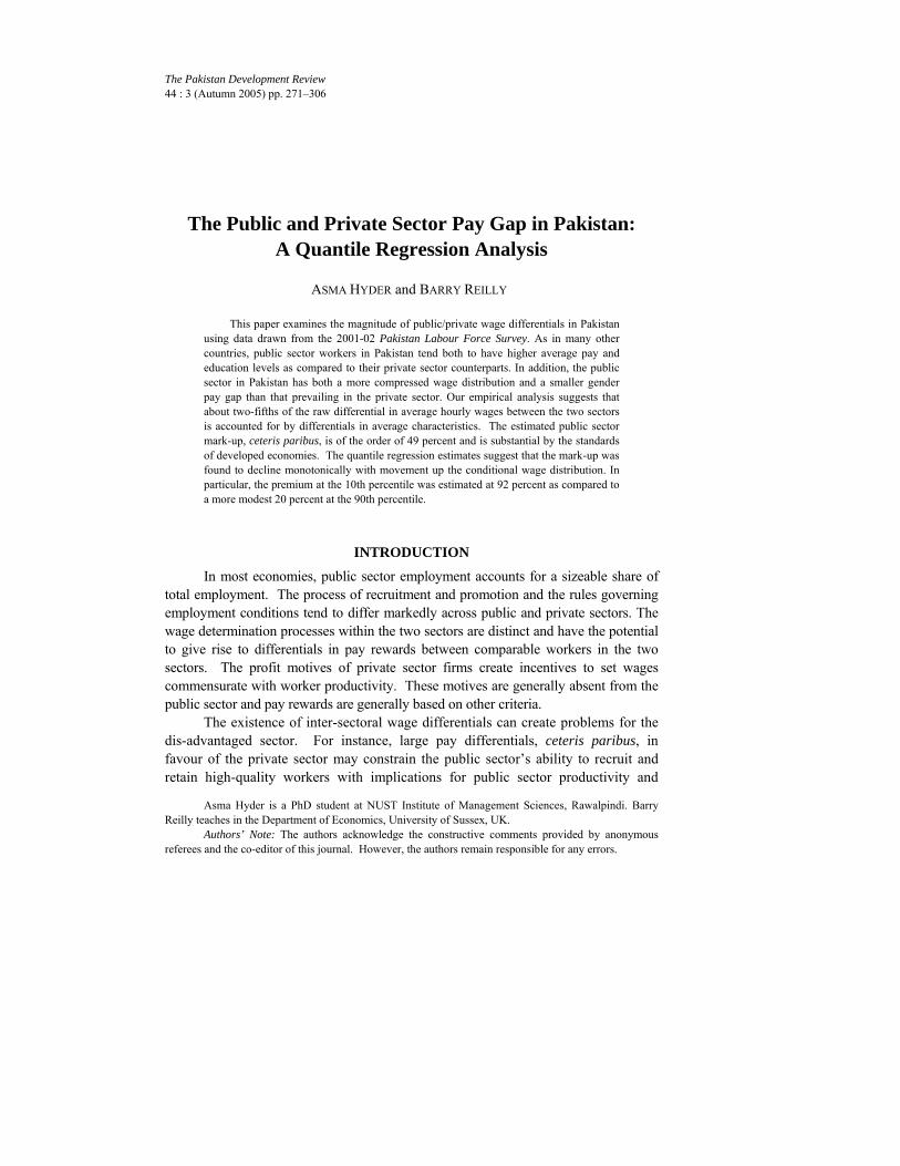
The Pakistan Development Review 44 : 3 (Autumn 2005) pp. 271–306

The Public and Private Sector Pay Gap in Pakistan:

A Quantile Regression Analysis

ASMA HYDER and BARRY REILLY*

This paper examines the magnitude of public/private wage differentials in Pakistan using data drawn from the 2001-02 Pakistan Labour Force Survey. As in many other countries, public sector workers in Pakistan tend both to have higher average pay and education levels as compared to their private sector counterparts. In addition, the public sector in Pakistan has both a more compressed wage distribution and a smaller gender pay gap than that prevailing in the private sector. Our empirical analysis suggests that about two-fifths of the raw differential in average hourly wages between the two sectors is accounted for by differentials in average characteristics. The estimated public sector mark-up, ceteris paribus, is of the order of 49 percent and is substantial by the standards of developed economies. The quantile regression estimates suggest that the mark-up was found to decline monotonically with movement up the conditional wage distribution. In particular, the premium at the 10th percentile was estimated at 92 percent as compared to a more modest 20 percent at the 90th percentile.

INTRODUCTION

In most economies, public sector employment accounts for a sizeable share of total employment. The process of recruitment and promotion and the rules governing employment conditions tend to differ markedly across public and private sectors. The wage determination processes within the two sectors are distinct and have the potential to give rise to differentials in pay rewards between comparable workers in the two sectors. The profit motives of private sector firms create incentives to set wages commensurate with worker productivity. These motives are generally absent from the public sector and pay rewards are generally based on other criteria.

The existence of inter-sectoral wage differentials can create problems for the dis-advantaged sector. For instance, large pay differentials, ceteris paribus, in favour of the private sector may constrain the public sector’s ability to recruit and retain high-quality workers with implications for public sector productivity and

Asma Hyder is a PhD student at NUST Institute of Management Sciences, Rawalpindi. Barry Reilly teaches in the Department of Economics, University of Sussex, UK.

Authors’ Note: The authors acknowledge the constructive comments provided by anonymous referees and the co-editor of this journal. However, the authors remain responsible for any errors.

Hyder and Reilly 272

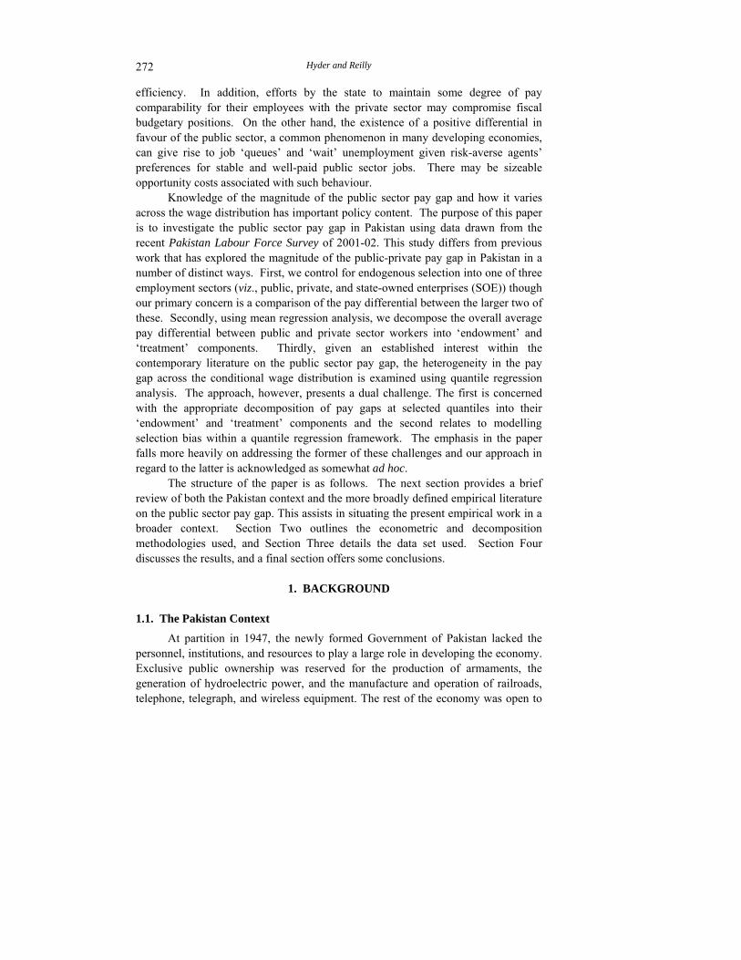
efficiency. In addition, efforts by the state to maintain some degree of pay comparability for their employees with the private sector may compromise fiscal budgetary positions. On the other hand, the existence of a positive differential in favour of the public sector, a common phenomenon in many developing economies, can give rise to job ‘queues’ and ‘wait’ unemployment given risk-averse agents’ preferences for stable and well-paid public sector jobs. There may be sizeable opportunity costs associated with such behaviour.

Knowledge of the magnitude of the public sector pay gap and how it varies across the wage distribution has important policy content. The purpose of this paper is to investigate the public sector pay gap in Pakistan using data drawn from the recent Pakistan Labour Force Survey of 2001-02. This study differs from previous work that has explored the magnitude of the public-private pay gap in Pakistan in a number of distinct ways. First, we control for endogenous selection into one of three employment sectors (viz., public, private, and state-owned enterprises (SOE)) though our primary concern is a comparison of the pay differential between the larger two of these. Secondly, using mean regression analysis, we decompose the overall average pay differential between public and private sector workers into ‘endowment’ and ‘treatment’ components. Thirdly, given an established interest within the contemporary literature on the public sector pay gap, the heterogeneity in the pay gap across the conditional wage distribution is examined using quantile regression analysis. The approach, however, presents a dual challenge. The first is concerned with the appropriate decomposition of pay gaps at selected quantiles into their ‘endowment’ and ‘treatment’ components and the second relates to modelling selection bias within a quantile regression framework. The emphasis in the paper falls more heavily on addressing the former of these challenges and our approach in regard to the latter is acknowledged as somewhat ad hoc.

The structure of the paper is as follows. The next section provides a brief review of both the Pakistan context and the more broadly defined empirical literature on the public sector pay gap. This assists in situating the present empirical work in a broader context. Section Two outlines the econometric and decomposition methodologies used, and Section Three details the data set used. Section Four discusses the results, and a final section offers some conclusions.

1. BACKGROUND 1.1. The Pakistan Context

At partition in 1947, the newly formed Government of Pakistan lacked the personnel, institutions, and resources to play a large role in developing the economy. Exclusive public ownership was reserved for the production of armaments, the generation of hydroelectric power, and the manufacture and operation of railroads, telephone, telegraph, and wireless equipment. The rest of the economy was open to

Public and Private Sector Pay Gap in Pakistan 273

private-sector development, and the government used many direct and indirect measures to stimulate or guide private-sector activities. The government enacted piecemeal measures between 1968 and 1971 to set minimum wages, promote collective bargaining for labour, reform the tax structure towards greater equity, and rationalise the salary structures. However, the implementation of these reforms was generally weak and uneven.

In 1972, the government nationalised thirty-two large manufacturing plants in eight major industries. The public sector expanded greatly in this period. In addition to the nationalisation of companies, government agencies were created to support various functions, such as the export of cotton and rice. Suitably qualified managers and technicians were scarce, a situation that became worse after 1974, when many of the more able left to seek higher salaries in the oil-producing countries of the Middle East. Labour legislation set high minimum wages and sizeable fringe benefits, boosting payroll costs in both public and private sectors.

After 1977, the government adopted a policy of greater reliance on private enterprises to achieve economic goals, and successive governments continued this policy throughout the late 1980s and the early 1990s. However, the government continued to play a large economic role in this period, with public-sector enterprises accounting for a significant portion of large-scale manufacturing. In 1991, it was estimated that such enterprises produced about 40 percent of national industrial output. As of early 1994, proposals to end state monopolies in selected industries were in various stages of implementation. Private investment no longer required government authorisation, except in sensitive industries. In early 1994, the government announced its intention to continue policies of both deregulation and liberalisation. The rise in the share of the private sector reflected the policy shift towards a market-based economy as well as the government’s weakened fiscal position.

In spite of the re-orientation of the economy towards the private sector in recent years, the competition for employment in the public sector remains keen in Pakistan. Public sector employment in Pakistan is still viewed as more attractive because of better pay, better working conditions, and the availability of other fringe benefits (e.g., pension rights and free medical benefits).

1.2. Empirical Literature Overview

The stylised facts offered on the public sector for developed economies, once wage determining characteristics are accounted for, are of a modest average positive wage gap in favour of public sector workers.1 In addition, public sector pay practice

1For example, see Blank (1994), Rees and Shah (1995), Disney and Gosling (1998) and Blackaby, Murphy and O’Leary (1999) for the UK; see Gyourko and Tracy (1988), Moulton (1990) and Blank (1994) for the US; see Lucifora and Meurs (2004) for UK, Italy and France. The evidence for Germany [see Dustmann and Van Soest (1998)] is less clear-cut and that for Holland suggests a negative ceteris paribus differential [see Van Ophem (1993)].


tends to attenuate the gender pay gap and narrow wage dispersion. The average effects, however, conceal variations in the performance of the public sector pay premium across the conditional wage distribution. In particular, a number of studies have documented a declining public sector pay premium in developed economies, with movement up the conditional wage distribution suggesting that public sector rewards are more substantial in the lower-paid jobs.2

The evidence for Latin America provides something of a contrast. Panizza (2000) examines the magnitude of the public/private sector pay gap for 17 countries over the 1980s and 1990s and reports average pay gaps that generally favour the private sector.3 Panizza (2000) also documents lower gender pay gaps in public sector labour markets. In addition, Falaris (2003), using micro-level data for Panama, confirmed both a weak mean public sector premium and effects that declined with movement up the conditional wage distribution. The evidence from Latin American countries tends to chime with what has emerged in transitional economies. The development of a buoyant private sector is generally viewed as a key part of a successful transformation to a market economy. The empirical literature on the ceteris paribus private sector wage premium in transitional economies is limited and beset by measurement issues4 but tends to suggest a positive wage premium in favour of private sector workers.5

There has been a modest volume of empirical work undertaken on the public sector pay gap for developing countries. Boudarbat (2004) notes a preference for public sector employment in Africa and a willingness among the educated to engage in ‘wait’ unemployment to secure the more well paid and stable public sector jobs. The author notes a sizeable public sector pay differential in Morocco for the highly educated. The earlier studies of Lindauer and Sabot (1983) for Tanzania and Van der Gaag, Stelcner, and Vijverberg (1989) for Cote D’Ivoire provide mixed evidence on the size and direction of the pay gap but the latter paper highlights the importance of selection bias in informing any reasonable interpretation. Terrell (1993), using data for Haiti, reports a relatively large average public sector pay gap with selection bias apparently relevant in only one sector. Al-Samarrai and Reilly (2005) detect no public sector wage effect using recent tracer survey data from Tanzania. Skyt-Neilsen and Rosholm (2001) detected a positive average ceteris paribus pay gap in

2For example, see Poterba and Rueben (1994) for the US; see Mueller (1998) for Canada; see Disney and Gosling (1998) and Blackaby, Murphy and O’Leary (1999) for the UK; see Lucifora and Meurs (2004) for Italy and France.

3Brazil was a notable exception here. This is not a surprise since public sector workers in Brazil are known to be well-paid [see Arbache, Dickerson, and Green (2004)].

4See Filer and Hanousek (2002) for problems related to the measurement of the private sector in transitional economies.

5See Newell and Socha (1998) and Adamchik and Bedi (2000) for Poland from the mid-1990s; see Lokshin and Jovanovic (2001) for a sample of Moscow workers; and see Krstic, Reilly and Tabet (2004) for a sample of Serbian workers.


favour of public sector workers in Zambia but noted that at the upper end of the conditional wage distribution it became negative for the highly educated. A recent study by Ajwad and Kurukulasuriya (2002), the primary focus of which was gender and ethnic wage disparities, detected no public sector pay premium either at the average or across selected quantiles of the conditional wage distribution for Sri Lanka. Finally, of direct relevance to our analysis, Nasir (2000), using data for Pakistan, detected a negligible differential in favour of public sector workers; but this study restricted the private sector comparator to the formal sector.

2. METHODOLOGY 2.1. Mean Regression Decompositions

The magnitude of the public sector pay premium could be crudely captured by using a pooled sample of data points on all workers in conjunction with the OLS procedure. If we assume a pooled sample of public and private sector data points and introduce the i subscripts for i=1,…,n, we could express the log wage equation with a simple intercept shift for the public sector as:

wi = Xi′β+ δGi + ui … … … … … (1)

where wi is the log wage for the ith individual; Xi is a k×1 vector of wage determining characteristics for the ith individual; β is a k×1 vector of the corresponding unknown parameters; Gi is a binary measure adopting a value of 1 if the individual is in the public sector and 0 otherwise and δ is its corresponding unknown parameter; ui is an error terms for the ith individual. The OLS estimate for δ provides the average ceteris paribus effect of being in a public sector job on the expected log wage.

The foregoing approach restricts the public sector premium to being captured by an intercept shift and ignores the fact that employment in the public sector may confer on the individual differential returns to, for example, education and experience. The conventional Blinder (1973) or Oaxaca (1973) methodology has been extensively used in this field to address this potential problem and readily extends to applications where the investigator wishes to decompose pay gaps between groups of workers using other qualitative indicators (e.g., race or employment sector). In our application, we are interested in decomposing the pay differential between public and private sector workers. The procedure involves the OLS estimation of separate sectoral wage equations and the use of the OLS coefficients in conjunction with the sectoral mean characteristics to compute explained (or ‘endowment’) and unexplained (or ‘treatment’) effects. The average mean difference in log wages ( D ) between two groups or sectors could be expressed as:


[ ] [ ]pspXspXsXwwD ps β−β′+β′−=−= ˆˆˆ … … (2)

where jw is the average logarithm of the wage for the jth employment sector; jX is

the vector of average characteristics for the jth employment sector; jβ̂ is the vector of

OLS wage determining coefficients for the jth employment sector; j = s, p where s denotes public (or state) sector and p denotes the private sector.6

The overall average differential in log wages between the two sectors is thus decomposable into differences in characteristics (as evaluated at the returns in the public sector) and differences in the estimated relationship between the two sectors (i.e., the sectoral differences in returns) evaluated at the mean set of private sector characteristics). It is clear that expression (2) could be re-cast using the ‘basket’ of average public sector characteristics as the use of an ‘index number’ approach is subject to the conventional ‘index number’ problem. However, given our application we believe the above decomposition provides the more meaningful basis for computing the mark-up of interest.

2.2. Quantile Regression Decompositions An exclusive focus on the average may provide a misleading impression as to the

variation in the magnitude of the ceteris paribus gender pay gap across the wage distribution. A number of different methods recently used in the literature allow for a more general counterfactual wage distributions under specific assumptions. These methods generally require relatively large sample sizes and are prohibitive in a context where the samples available tend to be modest.7 The quantile regression approach [e.g., see Chamberlain (1994); Buchinsky (1998)] provides a less data-demanding alternative, but one that can be informative about the impact of covariates at different points of the conditional wage distribution. In the use of a quantile regression model, the focus moves away from the mean to other selected points on the conditional wage distribution and the estimation procedure is formulated in terms of absolute rather than squared errors. The estimator is known as the Least Absolute Deviations (LAD) estimator.

If we again assume the pooled model in (1) above as a reasonable characterisation of the wage determining process, the median regression coefficients can be obtained by choosing the coefficient values that minimise L

L = ( ) ( )∑∑==

δ−β−δ−β−=δ−β−n

iiiiiiii

n

ii GXwsgnGXwGiXw

1

'''

1 … (3)

where sgn(a) is the sign of a, 1 if a is positive, and –1 if a is negative or zero.

6For expositional purposes, the third sector, the SOE sector, is ignored here given the paper’s primary emphasis. The relatively small sample size available for the SOE sector also restricts our discussion in the empirical section.

7For example, see DiNardo, Fortin, and Lemieux (1996), Fortin and Lemieux (1998), Donald, Green and Paarsch (2000) for a variety of different approaches.


The estimation of a set of conditional quantile functions potentially allows the delineation of a more detailed portrait of the relationship between the conditional wage distribution and the selected covariates (including public sector attachment). Given the linear formulation of the regression model, the coefficient estimates can be obtained using linear programming techniques. In contrast to the OLS approach, the quantile regression procedure is less sensitive to outliers and provides a more robust estimator in the face of departures from normality [see Koenker (2005) and Koenker and Bassett (1978)]. Quantile regression models may also have better properties than OLS in the presence of heteroscedasticity [see Deaton (1997)].

It is generally desirable to explore quantile regressions other than at the median. Using this same methodology, the log wage equation may be estimated conditional on a given specification and then calculated at various percentiles of the residuals (e.g., the 10th, the 25th, the 75th or the 90th) by minimising the sum of absolute deviations of the residuals from the conditional specification. In the context of the regression model specified, quantile regression estimation allows the estimation of the δ parameter at the 10th, 25th, 50th, 75th and 90th percentiles. The estimates obtained for δ allow us to establish the magnitude of the ceteris paribus gender pay gap at different points of the conditional wage distribution.

The asymptotic formula for the computation of the variance-covariance matrix is known to under-state the true variance covariance matrix in the presence of heteroscedasticity. The more conventional approach adopted to compute the variance-covariance matrix is the bootstrapping method, and this procedure is adopted in the empirical applications reported in this study.8

In the context of the estimation inherent in (3), the average ceteris paribus public sector pay gap is provided by the estimate for δ. Chamberlain (1994) used this type of model to explore the wage effect of unions at different points of the conditional wage distribution. However, the extensive literature on decomposing the mean pay gap, as emphasised in expression (2), employs separate wage equations for each sector. In the context of the estimation of quantile regression models by sector, the decomposition of the pay gap at different quantiles is not entirely straightforward. The decomposition within a quantile regression framework has been undertaken in a number of studies, [see Albrecht, Björklund, and Vroman (2003); Gardeazabal and Ugidos (2005) and Machado and Mata (2000)]. One of the key issues in any decomposition is to determine the appropriate realisation of characteristics with which to undertake the counterfactual exercise. In the linear mean regression model, it is intuitive to use mean characteristics. Although use of the mean characteristics is feasible with the estimated coefficients from quantile regressions, they may provide misleading realisations for the characteristics at points

8See Brownestone and Valletta (2001) for an accessible introduction to bootstrapping.


other than the conditional mean wage to which they relate. It seems more appropriate to use realisations that more accurately reflect the relevant points on the conditional wage distribution.

In order to appreciate this point more clearly, define the quantile regression for the public sector sub-sample as

ws = Xs′ βθs + uθs … … … … … … (4)

where Qθ(ws| Xs) = Xs′ βθs and Qθ(uθs | Xs) = 0 and θ denotes the particular quantile of interest. In addition, Xs is a k×n1 matrix of characteristics for the sample of public sector workers where n1 is the sample size, βθs is a k×1 vector of unknown parameters for the θth public sector regression quantile.

Define the quantile regression for the private sector sub-sample as:

wp = Xp′ βθp + uθp … … … … … … (5)

where Qθ(wp| Xp) = Xp′ βθp and Qθ(uθp | Xp) = 0. In this case Xp is a k×n2 matrix of characteristics for the sample of private sector workers where n2 is the sample size, βθp is a k×1 vector of unknown parameters for the θth private sector regression quantile.

Now:

Qθ(ws) = E[Xs | ws = Qθ(ws)]′ βθs + E[uθs | ws = Qθ(ws)] … … (6)

and

Qθ(wp) = E[Xp| wp = Qθ(wp)]′ βθp + E[uθp | wp = Qθ(wp)] … … (7)

where E(·) denotes the expectations operator. In this case E[uθs | ws = Qθ(ws)] ≠ 0 and E[uθp | wp= Qθ(wp)] ≠ 0. The characteristics used in (6) and (7) are evaluated conditionally at the unconditional log wage quantile value. In addition, the terms E[uθs | ws = Qθ(ws)] and E[uθp | wp = Qθ(wp)] are non-zero and provide an indication as to whether at a given quantile, the regression model over-predicts or under-predicts the log wage. These terms do not appear in the mean regression and thus, in a quantile regression decomposition, there will be some part of the pay gap left unassigned to either the ‘endowment’ or ‘treatment’ components at all quantiles of the conditional wage distribution.

We now turn to decomposing the public-private sector pay gap at different points of the conditional wage distribution. The pay gap at the θth quantile is defined as ∆θ and this can be decomposed into three parts:

∆θ = Qθ(ws) – Qθ(wp) = [ E[Xs | ws = Qθ(ws)] – E[Xp | wp = Qθ(wp)]]′ βθs

+ E[Xp | wp = Qθ(wp)]′[ βθs – βθs]

+ [E[uθs | ws = Qθ(ws)] – E[uθp | wp = Qθ(wp)]] … … (8)


This represents the quantile regression analogue to the mean decomposition reported in (2). The first part is the conventional ‘endowment’ part and gives the portion of the gap at the θth quantile explained by sectoral differences in the conditional mean characteristics at this point. The second part is the conventional ‘treatment’ component evaluated not at the unconditional mean (E[Xp]) but at a mean value conditional on the particular quantile value of the private sector log wage. The final component gives that portion of the difference in log wages not explained by the quantile regressions for the two sectors. In order to implement this procedure we need to compute the component parts of (8). We use an auxiliary regression approach based on Gardeazabal and Ugidos (2005). The approach is outlined in a technical appendix to this paper.

2.3. Selectivity Bias Issues

There is a selection issue for the analysis of the public sector pay gap and one that has been strongly emphasised in the literature based on mean regression analysis.9 Either through a process of self-selection by individuals or sample selection by employers, the location of individuals in either sector may not be interpretable as the outcome of a random process. In the context of the mean regression model Heckman (1979) and Lee (1983) provide well-known solutions.

As noted by Neuman and Oaxaca (2004), selectivity correction procedures introduce a number of ambiguities for standard wage decomposition analysis. The wage decomposition favoured by many authors10 in the presence of such a correction is usually expressed as

[ ] [ ] [ ]ppsspspspsps XXXwwD λτ−λτ+β−β′+β′−=−= ˆˆˆˆˆ … (9)

where everything is defined as in (2) above but with jτ̂ now representing the OLS

estimate of the j selection parameter, one for each employment sector, and jλ is the

sample averaged selection variable for the jth employment group computed as the inverse of the Mills ratio term using estimates from a probit model for sectoral attachment as per Heckman (1979) or through the Lee (1983) term based on use of a multinomial logit model.

Currently, there is little consensus regarding the most appropriate correction procedure for selectivity bias in quantile regression models. Buchinsky (1999) uses the work of Newey (1999) to approximate the selection term by a higher order series expansion. The power series is based on the inverse Mills ratio (or its Lee

9See Gyourko and Tracy (1988), Van der Gaag and Vijerberg (1988), and Terrell (1993). 10For instance, Reimers (1983) who nets the selection differences out of the overall pay gap to

generate wage offer differentials.


equivalent).11 This approach has the potential pitfall that the wage regression intercept term is not identified given its conflation with the constant term associated with the higher order series that proxies for the selection bias.12 Given the lack of consensus and problems associated with introducing higher order selection terms into quantile regression models, we adopt the rather crude expedient of inserting the simple selection terms into the quantile regression models. It is acknowledged that, in contrast to the mean regression case, this provides an inexact correction for selection bias. However, it circumvents the tricky problem of identifying the wage regression constant term.

We now turn to decomposing the public-private sector pay gap at different points of the conditional wage distribution having corrected for selection bias. The pay gap at the θth quantile is now decomposed into four parts:

∆θ = Qθ(ws) – Qθ(wp)

= [E[Xs | ws = Qθ(ws)] – E[Xp | wp = Qθ(wp)]]′ βθs

+ E[Xp | wp = Qθ(wp)]′[βθs – βθs]

+ [τθs E[λs| ws = Qθ(ws)] – [τθp E[λp| ws = Qθ(ws)]]

+ [E[uθs | ws = Qθ(ws)] – E[uθp | wp = Qθ(wp)]] … … (10)

where the third component is the selection effect. Finally, in order to address the problem of selectivity bias we exploit the

procedure developed by Lee (1983), as used by Gyourko and Tracy (1988) in a similar application, which provides a more general approach to the correction of selectivity bias than that originally offered by Heckman (1979). The procedure is two-step but exploits estimates from a multinomial logit model (MNL) rather than a probit to construct the set of selection correction terms. The estimation of models with selection effects always contains difficulties. In addition, their identification is always a demanding task. The eminently sensible advice of Gyourko and Tracy (1988) to compute and report both corrected and uncorrected differentials is adhered to in this study.13

3. DATA

This study uses cross-section data drawn from the nationally representative Labour Force Survey (LFS) for Pakistan for 2001-2. The working sample used is based on those in wage employment and comprises a total of 7352 workers once missing values and unusable observations are discarded. This total consists of 3694, 3310 and 348 workers in the private, public and state owned enterprise (SOE) sectors respectively. The government sector includes federal government, provincial

11See also Fitzenberger (2003) for an alternative approach. 12Heckman (1990) and Andrews and Shafgans (1998) suggest solutions to this problem. 13In order to conserve space, the MNL estimates are not reported in this study.


government and local bodies. State owned enterprises (SOEs) are defined as public enterprises and public limited companies. Thus, over one-half of waged employees are in the public sector.

The private sector is defined here to include workers employed in private limited companies, cooperative societies, individual ownership and partnerships. It is sometimes argued that, in an analysis of the public/private sector pay gap in developing countries, it is desirable to disaggregate the private sector into formal and informal sectors.14 This is largely a matter of investigator preference and our approach is to retain a sufficiently broad definition of the private sector. Any dis-aggregation of the private sector along such lines is likely to be prone to potential misclassification and measurement error, and is thus eschewed in this study.

The data collection for the LFS is spread over four quarters of the year in order to capture any seasonal variations in activity. The survey covers all urban and rural areas of the four provinces of Pakistan as defined by the 1998 Population Census. The LFS excludes the federally Administered Tribal Areas (FATA), military restricted areas, and protected areas of NWFP. These exclusions are not seen as significant since the relevant areas constitute about 3 percent of the total population of Pakistan.

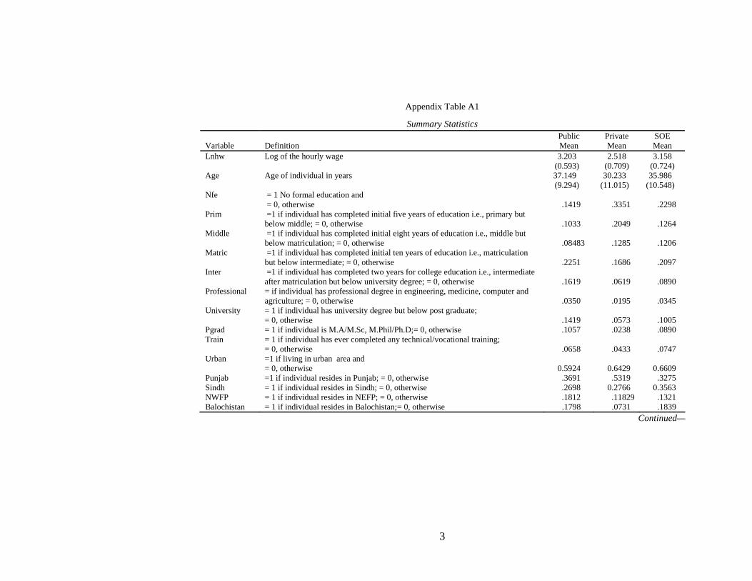
Table A1 of the appendix presents the summary statistics and definitions of the variables used in our analysis. The natural logarithm of the hourly wage15 is used

as the dependent variable. Table A1 highlights the fact that the public and SOE sectors are relatively high pay sectors with large concentrations of professionals, graduates and postgraduates. A detailed dis-aggregation of educational qualifications is used in our analysis and this facilitates the computation of private rates of returns to these qualifications.

In order to examine the relationship between earnings and age from the perspective of human capital theory, age and its quadratic are used in the specifications.16 These measures are actually designed to proxy for labour force experience, which cannot be accurately measured using our data source. Our analysis is restricted to those aged between 15 and 60 years of age. This facilitates a more worthwhile comparison between public and private sector workers. The marital status of a respondent is divided into three mutually exclusive categories (viz., “married”, “never married” and “widow and divorced”). The settlement type within which the individual resides is captured by a binary control for residing in an urban area. Four regional controls are included and these correspond to the four provinces in Pakistan (viz., Punjab, Balochistan, Sindh and NWFP). A set of controls capturing

14This was the approach adopted by Nasir (2000), using data drawn from an earlier round of the LFS.

15The hourly wages expressed in rupees, were calculated by dividing weekly earnings by the number of hours worked per week.

16The use of age and its quadratic also renders the construction of the conditional vector of characteristics at different quantiles somewhat easier.


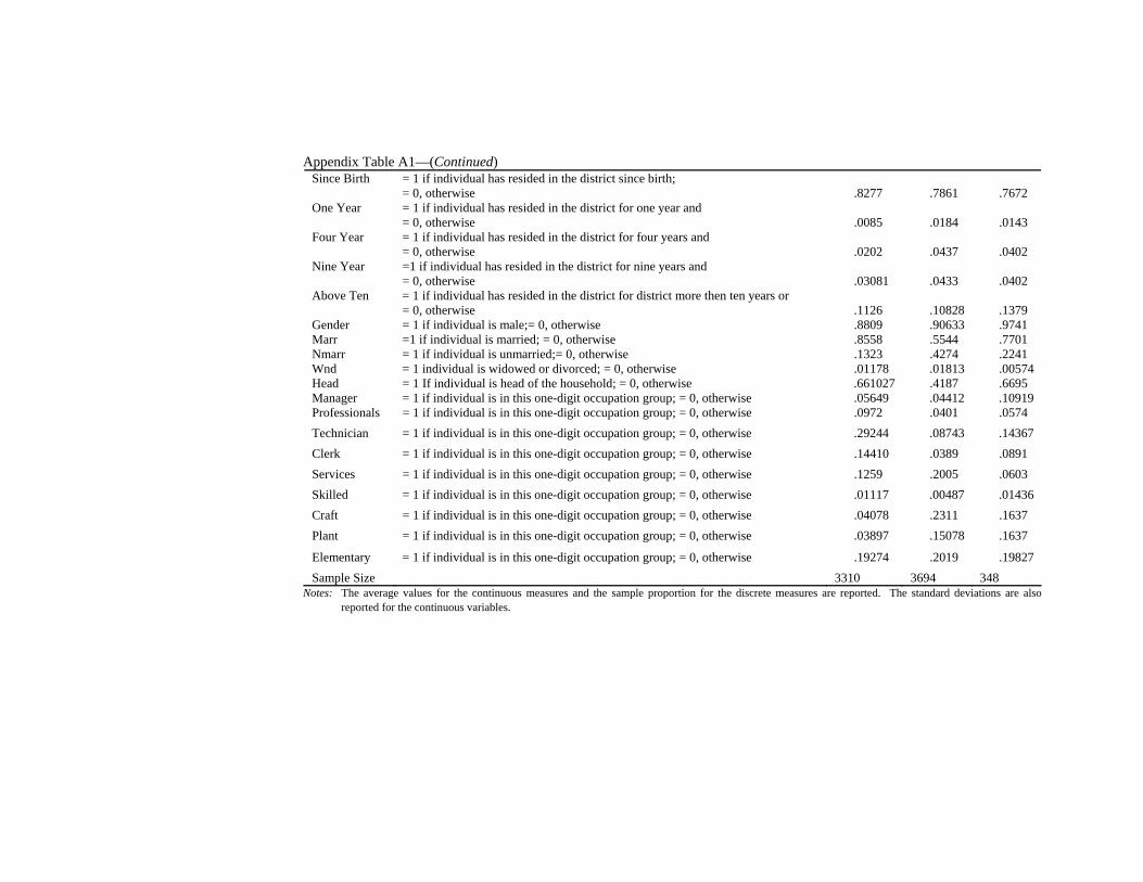
the time the respondent spent in the current district is also included in our analysis. The notion here is that location specific human capital and social networks may be important in the wage determination process. This may be particularly relevant in the private sector.

It is an established fact that an individual’s occupation is a very important determinant of their earnings. Nine one-digit occupational categories, defined according to the standard classification of occupations, are thus included in our specifications. As reported in Table A1, the public sector is characterised by a high proportion of technicians and skilled professionals. However, in the private sector there is a higher concentration of craft and related trade workers.

Female labour force participation is low in Pakistan. On the basis of our sample only 12 percent of public sector employees and about 3 percent of those in private sector waged employment are women. The inclusion of women in our empirical analysis is a judgment call. A sub-theme of our analysis is to explore the impact that public sector employment exerts on the gender pay gap. The use of an intercept shift to capture gender helps inform this issue, though perhaps imperfectly. We are particularly interested in examining the extent to which the public sector in Pakistan attenuates the gender pay gap and the extent to which there is evidence of a ‘glass ceiling’ in either of these two sectors.

It is important to note that Labour Force Survey does not provide information regarding fringe benefits received by workers. Thus our analysis is restricted to a wage gap defined in monetary terms. If these additional pecuniary measures (e.g., fringe benefits) and other non-pecuniary factors (e.g., working conditions and stability of employment) are allowed for, the estimated public-private premium is likely to be even larger than our estimates reported here. There is some evidence that this is indeed the case in other countries. For example, Ichniowski (1980) found the relative union/non-union fringe benefit differentials for fire-fighters to be roughly four times as large as the comparable wage differentials. The magnitude is much larger than that found by Freeman (1981) in his public/private sector studies. It would be desirable to have information regarding labour market fringe benefits available in the Labour Force Survey. The availability of such information would enhance understanding about the true magnitude of the inter-sectoral differentials between the public and private sectors. However, in the absence of such data our results carry a caveat and should be taken to reflect the lower limit of the inter-sectoral differential between public and private sector workers.

4. EMPIRICAL RESULTS

The specified wage equations included controls for highest education qualification attained, whether an individual undertook technical training, age and its quadratic, martial status, gender, settlement type, a set of regional controls, a set of


dummies for the length of time resident in the district, and a set of one-digit occupational controls. For brevity, only the estimates relating to the education, age gender, and sectoral attachment are reported in the tables. Table 1 reports the estimates for a pooled regression model based on expression (1) where the public sector enters as an intercept shift and provides an estimate of the public sector ceteris paribus mark-up relative to the broadly defined private sector base. Estimates for a mean regression and models estimated at selected quantiles of the conditional wage distribution are also recorded in this table. In addition, estimates for an inter-quantile regression model based on differences between the 90th and 10th quantiles are reported.

The mean regression estimates suggest a sizeable premium to both graduate and postgraduate qualifications in the Pakistan labour market.17 There is also a modest premium of just over 5 percent associated with having undertaken technical training. Women appear to encounter a significant disadvantage in the labour market. Men, on average and ceteris paribus, earn approximately 33 percent more than women in terms of hourly wages. Although the estimated signs on the linear and quadratic terms in age are consistent with human capital theory, the turning-point is implausible. This suggests that, at the average, wages and earnings are better specified as being linearly related.18 The estimates for the quantile regression model at the median are broadly in comport with the mean regression results and this could be taken to imply that outliers exert little influence on our mean estimates. The inter-quantile regression coefficients reveal that holding postgraduate qualifications and undertaking training have stronger effects at the top end of the conditional wage distribution than at the bottom end and this might have implications for wage inequality. In contrast to a substantial literature on the ‘glass ceiling’ from developed economies, there is little evidence from the quantile regression estimates that the gender effect increases with movement across the conditional wage distribution. On the contrary, the evidence from Pakistan is that the ceteris paribus gender pay gap declines across the wage distribution with the inter-quantile regression estimates suggesting a decline of almost 30 percent between the 90th and 10th percentiles. Thus, women in the higher paid jobs in Pakistan are not as disadvantaged as many of their western counterparts.19

The pooled regression model provides a framework for computing the public sector pay premium as per expression (1). The average ceteris paribus mark-up relative to the private sector is estimated of the order of 45 percent. This premium declines sharply with movement up the conditional wage distribution, a fact consistent with the existing literature on the public sector pay gap in developed

17The average annualised rate of return to a professional qualification, an undergraduate degree, and a postgraduate degree are 9.2 percent, 9.1 percent, and 10.8 percent respectively.

18Alternatively, the age measure could be expressed using splines. 19For example, see Albrecht, Björklund, and Vroman (2003) for the case of Sweden.

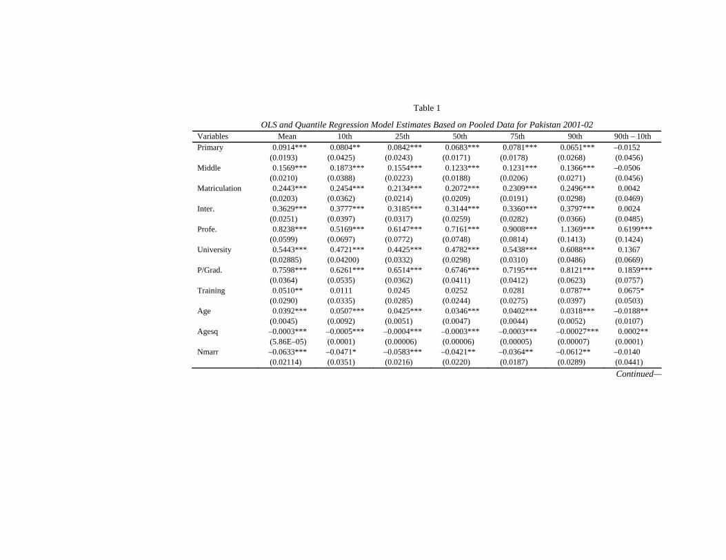
Table 1

OLS and Quantile Regression Model Estimates Based on Pooled Data for Pakistan 2001-02 Variables Mean 10th 25th 50th 75th 90th 90th – 10th Primary 0.0914***

(0.0193) 0.0804**

(0.0425) 0.0842***

(0.0243) 0.0683***

(0.0171) 0.0781***

(0.0178) 0.0651***

(0.0268) –0.0152 (0.0456)

Middle 0.1569*** (0.0210)

0.1873*** (0.0388)

0.1554*** (0.0223)

0.1233*** (0.0188)

0.1231*** (0.0206)

0.1366*** (0.0271)

–0.0506 (0.0456)

Matriculation 0.2443*** (0.0203)

0.2454*** (0.0362)

0.2134*** (0.0214)

0.2072*** (0.0209)

0.2309*** (0.0191)

0.2496*** (0.0298)

0.0042 (0.0469)

Inter. 0.3629*** (0.0251)

0.3777*** (0.0397)

0.3185*** (0.0317)

0.3144*** (0.0259)

0.3360*** (0.0282)

0.3797*** (0.0366)

0.0024 (0.0485)

Profe. 0.8238*** (0.0599)

0.5169*** (0.0697)

0.6147*** (0.0772)

0.7161*** (0.0748)

0.9008*** (0.0814)

1.1369*** (0.1413)

0.6199*** (0.1424)

University 0.5443*** (0.02885)

0.4721*** (0.04200)

0.4425*** (0.0332)

0.4782*** (0.0298)

0.5438*** (0.0310)

0.6088*** (0.0486)

0.1367 (0.0669)

P/Grad. 0.7598*** (0.0364)

0.6261*** (0.0535)

0.6514*** (0.0362)

0.6746*** (0.0411)

0.7195*** (0.0412)

0.8121*** (0.0623)

0.1859*** (0.0757)

Training 0.0510** (0.0290)

0.0111 (0.0335)

0.0245 (0.0285)

0.0252 (0.0244)

0.0281 (0.0275)

0.0787** (0.0397)

0.0675* (0.0503)

Age 0.0392*** (0.0045)

0.0507*** (0.0092)

0.0425*** (0.0051)

0.0346*** (0.0047)

0.0402*** (0.0044)

0.0318*** (0.0052)

–0.0188** (0.0107)

Agesq –0.0003*** (5.86E–05)

–0.0005*** (0.0001)

–0.0004*** (0.00006)

–0.0003*** (0.00006)

–0.0003*** (0.00005)

–0.00027*** (0.00007)

0.0002** (0.0001)

Nmarr –0.0633*** (0.02114)

–0.0471* (0.0351)

–0.0583*** (0.0216)

–0.0421** (0.0220)

–0.0364** (0.0187)

–0.0612** (0.0289)

–0.0140 (0.0441) Continued—

Table 1—(Continued) Wnd –0.0165

(0.0534) –0.0425 (0.0935)

–0.0109 (0.0780)

0.0163 (0.0503)

–0.0156 (0.0458)

–0.0194 (0.0843)

0.0231 (0.1234)

Gender 0.2838*** (0.0259)

0.5024*** (0.0622)

0.3644*** (0.0321)

0.2128*** (0.0281)

0.1596*** (0.0294)

0.1470*** (0.0275)

–0.3554*** (0.0697)

Public 0.3747*** (0.0151)

0.5621*** (0.0255)

0.4563*** (0.0163)

0.3686*** (0.0166)

0.2762*** (0.0159)

0.1878*** (0.0237)

–0.3743*** (0.0315)

SOE 0.3339*** (0.0301)

0.3508*** (0.0585)

0.3529*** (0.0382)

0.3520*** (0.0292)

0.2914*** (0.0307)

0.3037*** (0.0600)

–0.0471 (0.0791)

Constant 1.2043*** (0.0908)

0.1870 (0.1774)

0.8186*** (0.1045)

1.4155*** (0.0906)

1.6261*** (0.0916)

2.0666*** (0.1161)

1.8795** (0.2157)

R2/Psuedo–R2 0.5312 0.3202 0.3434 0.3564 0.3783 0.4006 N/a Sample Size 7352 7352 7352 7352 7352 7352 7352

Notes: (a) ***, ** and * denote statistical significance at the 1 percent, 5 percent and 10 percent level respectively using two-tailed tests. (b) Wage equation specifications also include controls for residing in an urban settlement, four provincial controls, eight occupation controls, and four

controls capturing the time spent in the district of residence. (c) Standard errors are in parentheses. The OLS standard errors are based on Huber (1967) and the quantile regression model estimates are based on

bootstrapping with 200 replications.


economies. In the lowest paid jobs located at the 10th percentile of the conditional wage distribution, the mark-up is computed at 92 percent compared to a more modest 21 percent in the higher paid jobs at the 90th percentile. The inter-quantile regression estimates confirms that these differentials are statistically different from each other at a conventional level of statistical significance. This finding serves to highlight the wage compressing labour market effects of the public sector in Pakistan.20

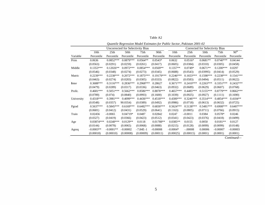
Our attention now turns to the results from separate estimation of the public and private sector wage equations and the computation of the ‘mark-ups’ using expressions (2) and (9) for the mean regressions and expressions (8) and (10) for the quantile regressions. Tables A2 to A5 in the Appendix report the sectoral wage equation estimates with and without corrections for selection bias.21 The estimates are not discussed in detail here, though a number of points are worth making about the mean regression estimates. Firstly, the returns to the higher educational qualifications are generally lower in the public compared to the private sector. This is particularly valid for professional qualifications and undergraduate degrees (see Table A6). On average, it would appear that the more highly qualified public sector workers trade-off substantial wage returns for the security and other non-wage benefits associated with the public sector.22 Secondly, and as encountered in the pooled regression model, the use of the quadratic in age in the public sector generates an implausible turning point. This indicates that, in this particular case, the linear effect is considerably more important and suggests that in the public sector pay and age are linked in a very strong linear fashion. Thirdly, the gender pay gap in favour of males is considerably lower in the public sector (16 percent) compared to the private sector (53 percent), and this is true at all selected quantiles of the conditional wage distribution.

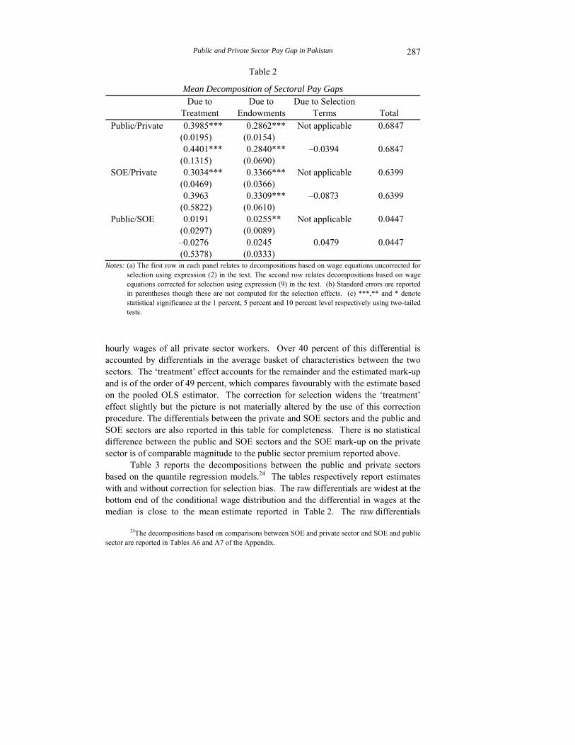
Table 2 reports the decomposition of the mean public/private sector pay gap. The estimates are based on models with and without correction for selection. In raw terms the average gap in log hourly wages between the public and private sector is 0.685.23 In other words, public sector worker earn, on average, almost double the

20The SOE effect is comparable to the public sector effect in the mean regression but exhibits a greater degree of stability across the conditional wage distribution as confirmed by the inter-quantile regression estimate. However, the small sample size merits extreme caution in interpreting the quantile regression estimates.

21There is marginal evidence that selection bias is an issue for our estimates. This may reflect the quality of the instruments used for our empirical analysis. However, there is a dearth of good instruments available in the dataset and this is the best that can be done under the circumstances.

22For instance, the rate of return to a professional qualification is nearly seven percentage points lower in the public sector and over 11 percentage points lower for an undergraduate degree holder than in the private sector.

23This is in contrast to Nasir (2000) who found little difference in overall wages between the public sector and the formal private sector and negative treatment effects. This work is not directly comparable to our analysis given that we do not distinguish between formal and informal segments of the private sector.


Table 2

Mean Decomposition of Sectoral Pay Gaps

Due to

Treatment Due to

Endowments Due to Selection

Terms Total Public/Private 0.3985***

(0.0195) 0.2862***

(0.0154) Not applicable 0.6847

0.4401*** (0.1315)

0.2840*** (0.0690)

–0.0394 0.6847

SOE/Private 0.3034*** (0.0469)

0.3366*** (0.0366)

Not applicable 0.6399

0.3963 (0.5822)

0.3309*** (0.0610)

–0.0873 0.6399

Public/SOE 0.0191 (0.0297)

0.0255** (0.0089)

Not applicable 0.0447

–0.0276 (0.5378)

0.0245 (0.0333)

0.0479 0.0447

Notes: (a) The first row in each panel relates to decompositions based on wage equations uncorrected for selection using expression (2) in the text. The second row relates decompositions based on wage equations corrected for selection using expression (9) in the text. (b) Standard errors are reported in parentheses though these are not computed for the selection effects. (c) ***,** and * denote statistical significance at the 1 percent, 5 percent and 10 percent level respectively using two-tailed tests.

hourly wages of all private sector workers. Over 40 percent of this differential is accounted by differentials in the average basket of characteristics between the two sectors. The ‘treatment’ effect accounts for the remainder and the estimated mark-up and is of the order of 49 percent, which compares favourably with the estimate based on the pooled OLS estimator. The correction for selection widens the ‘treatment’ effect slightly but the picture is not materially altered by the use of this correction procedure. The differentials between the private and SOE sectors and the public and SOE sectors are also reported in this table for completeness. There is no statistical difference between the public and SOE sectors and the SOE mark-up on the private sector is of comparable magnitude to the public sector premium reported above.

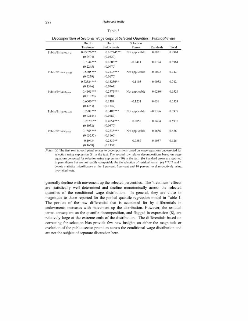
Table 3 reports the decompositions between the public and private sectors based on the quantile regression models.24 The tables respectively report estimates with and without correction for selection bias. The raw differentials are widest at the bottom end of the conditional wage distribution and the differential in wages at the median is close to the mean estimate reported in Table 2. The raw differentials

24The decompositions based on comparisons between SOE and private sector and SOE and public sector are reported in Tables A6 and A7 of the Appendix.


Table 3

Decomposition of Sectoral Wage Gaps at Selected Quantiles: Public/Private

Due to

Treatment Due to

Endowments Selection

Terms Residuals Total

Public/Privateθ=0.10 0.65026*** (0.0504)

0.16274*** (0.0320)

Not applicable 0.0831 0.8961

0.7044*** (0.2245)

0.1603** (0.0970)

–0.0411 0.0724 0.8961

Public/Private θ=0.25 0.5305*** (0.0239)

0.2138*** (0.0170)

Not applicable –0.0022 0.742

0.72524*** (0.1546)

0.13236** (0.0764)

–0.1103 –0.0052 0.742

Public/Private θ=0.5 0.4105*** (0.01870)

0.2775*** (0.0781)


0.6000*** (0.1253)

0.1384 (0.1547)

–0.1251 0.039 0.6524

Public/Private θ=0.75 0.2881*** (0.02144)

0.3483*** (0.0187)


0.23796** (0.1032)

0.4054*** (0.0670)

–0.0052 –0.0404 0.5978

Public/Private θ=0.9 0.1865*** (0.03255)

0.2738*** (0.1166)


0.19434 (0.1668)

0.2839** (0.1357)

0.0389 0.1087 0.626

Notes: (a) The first row in each panel relates to decompositions based on wage equations uncorrected for selection using expression (8) in the text. The second row relates decompositions based on wage equations corrected for selection using expression (10) in the text. (b) Standard errors are reported in parentheses but are not readily computable for the selection of residual terms. (c) ***,** and * denote statistical significance at the 1 percent, 5 percent and 10 percent level respectively using two-tailed tests.

generally decline with movement up the selected percentiles. The ‘treatment’ effects are statistically well determined and decline monotonically across the selected quantiles of the conditional wage distribution. In general, they are close in magnitude to those reported for the pooled quantile regression model in Table 1. The portion of the raw differential that is accounted for by differentials in endowments increases with movement up the distribution. However, the residual terms consequent on the quantile decomposition, and flagged in expression (8), are relatively large at the extreme ends of the distribution. The differentials based on correcting for selection bias provide few new insights on either the magnitude or evolution of the public sector premium across the conditional wage distribution and are not the subject of separate discussion here.


CONCLUSIONS

Public sector employment accounts for over one-half of waged employment in Pakistan. The empirical analysis undertaken in this study for Pakistan tends to concur with the summary consensus offered by Gregory and Borland (1999) on public sector labour markets in developed countries. As elsewhere, public sector workers in Pakistan tend to have both higher average pay and education levels as compared to their private sector counterparts. In addition, the public sector in Pakistan has a more compressed wage distribution and a smaller gender pay gap than that prevailing in the private sector.

Our empirical analysis suggests that about two-fifths of the raw differential in average wages between the public and private sector is accounted by differentials in average characteristics. The estimated ceteris paribus public sector mark-up is of the order of 49 percent and is substantial by the standards of developed economies. The mark-up was found to decline monotonically with movement up the conditional wage distribution. In particular, the premium at the 10th percentile was estimated at 92 percent as compared to a more modest 20 percent at the 90th percentile.

The existence of a sizeable public-private sector differential has obvious implications for the Pakistan labour market and can create ‘queues’ for public sector jobs given they are comparatively well-paid across a spectrum of low- and high-paid jobs. An obvious agenda for future research would be to investigate the extent to which these differentials influence sectoral attachment and give rise to the phenomenon of ‘wait’ unemployment.

Finally, employment in the public sector is generally viewed as an attractive option in Pakistan not only because of the wage differentials documented in this study but also as a consequence of the perquisites, such as housing, free telephone provision for civil servants, job security, free medical benefits, etc., associated with employment in this sector. Public sector employment in Pakistan could be interpreted as providing rent-seeking opportunities for some. The tax-payer is not represented at the negotiating table and the state bureaucracy has an incentive to conceal the nature and magnitude of spending on such fringe benefits. The expenditure on fringe benefits impacts strongly on the national exchequer but also bestows an unfair advantage on the public sector relative to the private sector. This subsidised advantage curtails the potential for the private sector’s development, a key ingredient for an economy’s transformation and its sustainable long-term economic growth. One issue that warrants consideration for future research in this area would be an investigation into the magnitude of such fringe benefits in Pakistan and their contribution to the more broadly defined public-private sector differential. It would be informative to investigate within this framework the likely cost implications to the national exchequer if fringe benefits were actually replaced by cash payments. It is an empirical question whether such a policy would reduce the overall cost to the exchequer, but it would certainly introduce a greater degree of transparency to public sector spending.


Appendices

TECHNICAL APPENDIX

In order to illustrate the computation of vectors for the realisations of explanatory variables conditional on log wage quantile values using the Gardeazabal and Ugidos (2005) method, we use decomposition (8) reported in the text.

(1) Qθ(ws) and Qθ(wp) are easily computed. For example, the quantile regression of log public (private) sector wages on a constant term yields the relevant log wage at the particular quantile for the public (private) sector.

(2) The quantile regression procedure outlined above yields estimates for the parameter vectors (βθs and βθp).

(3) The computation of the conditional expectation terms E[Xs | ws = Qθ(ws)] and E[Xp | wp = Qθ(wp)] involves a bit more work. We need to distinguish between three types of explanatory variables generally used in a wage specification. These are: (i) continuous explanatory variables; (ii) single binary explanatory variables; and (iii) sets of mutually exclusive binary explanatory variables. These three cases are now examined in turn.

(i) Continuous Explanatory Variables

In this case we regress the continuous explanatory variable (e.g., age) on the log of the wage using a linear bivariate regression. Assume the following model is estimated by OLS using the sub-sample of private sector workers:

Agei = α0 + α1wi+ ui

In order to compute the age conditional on the log wage at the θth quantile, we evaluate:

[ ] )(ˆˆ)(ˆ10 ppi wQwpQwAgeE θθ α+α==

where the wage value used in the OLS regression is the private sector log wage at the θth quantile. The conditional mean now gives us the predicted private sector age at the θth quantile’s private sector log wage. A similar exercise can then be undertaken to obtain the conditional expectation using the public sector log wage. (ii) A Single Binary Variable

In this case, we use a logit model and regress the single binary variable (e.g., gender) on the log of the wage using the sub-sample of private sector workers. Then:

[ ] [ ] )(ˆˆ)(ˆ10 pp wQFwpQwgenderE θθ γ+γ==


where F represents the CDF for the logistic and 0γ̂ and 1γ̂ represent the relevant maximum likelihood logit coefficient estimates. The wage value used in conjunction with these estimates is the private sector log wage at the θth quantile. A similar exercise can again be undertaken to obtain the conditional expectation using the public sector log wage. (iii) A Set of Mutually Exclusive Binary Variables

In this case, we use a multinomial logit model and regress the variable with say k outcomes (e.g., occupation coded 1, 2, 3..., k) on the private sector log wage. The multinomial logit coefficients are then used to compute predicted outcomes at the different quantiles of the public (or public) sector log wage. Gardeazabal and Ugidos (2005) suggest the use of a binary regression model for all binary variables. We argue that it is more appropriate to use a multiple outcome model where the outcomes relate to a set of mutually exclusive binary variables.

(4) The final component of the decomposition can then be computed as a residual given that the remainder of the information is already available through steps 1 to 3 above.

3

Appendix Table A1

Summary Statistics Public Private SOE Variable Definition Mean Mean Mean Lnhw

Log of the hourly wage 3.203 (0.593)

2.518 (0.709)

3.158 (0.724)

Age Age of individual in years 37.149 (9.294)

30.233 (11.015)

35.986 (10.548)

Nfe

= 1 No formal education and = 0, otherwise .1419 .3351 .2298

Prim

=1 if individual has completed initial five years of education i.e., primary but below middle; = 0, otherwise .1033 .2049 .1264

Middle

=1 if individual has completed initial eight years of education i.e., middle but below matriculation; = 0, otherwise .08483 .1285 .1206

Matric

=1 if individual has completed initial ten years of education i.e., matriculation but below intermediate; = 0, otherwise .2251 .1686 .2097

Inter

=1 if individual has completed two years for college education i.e., intermediate after matriculation but below university degree; = 0, otherwise .1619 .0619 .0890

Professional = if individual has professional degree in engineering, medicine, computer and agriculture; = 0, otherwise .0350 .0195 .0345

University

= 1 if individual has university degree but below post graduate; = 0, otherwise .1419 .0573 .1005

Pgrad = 1 if individual is M.A/M.Sc, M.Phil/Ph.D;= 0, otherwise .1057 .0238 .0890 Train

= 1 if individual has ever completed any technical/vocational training; = 0, otherwise .0658 .0433 .0747

Urban

=1 if living in urban area and = 0, otherwise 0.5924 0.6429 0.6609

Punjab =1 if individual resides in Punjab; = 0, otherwise .3691 .5319 .3275 Sindh = 1 if individual resides in Sindh; = 0, otherwise .2698 0.2766 0.3563 NWFP = 1 if individual resides in NEFP; = 0, otherwise .1812 .11829 .1321 Balochistan = 1 if individual resides in Balochistan;= 0, otherwise .1798 .0731 .1839

Continued—

Appendix Table A1—(Continued) Since Birth = 1 if individual has resided in the district since birth;

= 0, otherwise .8277 .7861 .7672 One Year = 1 if individual has resided in the district for one year and

= 0, otherwise .0085 .0184 .0143 Four Year = 1 if individual has resided in the district for four years and

= 0, otherwise .0202 .0437 .0402 Nine Year =1 if individual has resided in the district for nine years and

= 0, otherwise .03081 .0433 .0402 Above Ten = 1 if individual has resided in the district for district more then ten years or

= 0, otherwise .1126 .10828 .1379 Gender = 1 if individual is male;= 0, otherwise .8809 .90633 .9741 Marr =1 if individual is married; = 0, otherwise .8558 .5544 .7701 Nmarr = 1 if individual is unmarried;= 0, otherwise .1323 .4274 .2241 Wnd = 1 individual is widowed or divorced; = 0, otherwise .01178 .01813 .00574 Head = 1 If individual is head of the household; = 0, otherwise .661027 .4187 .6695 Manager = 1 if individual is in this one-digit occupation group; = 0, otherwise .05649 .04412 .10919 Professionals = 1 if individual is in this one-digit occupation group; = 0, otherwise .0972 .0401 .0574 Technician = 1 if individual is in this one-digit occupation group; = 0, otherwise .29244 .08743 .14367 Clerk = 1 if individual is in this one-digit occupation group; = 0, otherwise .14410 .0389 .0891 Services = 1 if individual is in this one-digit occupation group; = 0, otherwise .1259 .2005 .0603 Skilled = 1 if individual is in this one-digit occupation group; = 0, otherwise .01117 .00487 .01436 Craft = 1 if individual is in this one-digit occupation group; = 0, otherwise .04078 .2311 .1637 Plant = 1 if individual is in this one-digit occupation group; = 0, otherwise .03897 .15078 .1637

Elementary = 1 if individual is in this one-digit occupation group; = 0, otherwise .19274 .2019 .19827 Sample Size 3310 3694 348

Notes: The average values for the continuous measures and the sample proportion for the discrete measures are reported. The standard deviations are also reported for the continuous variables.

5

Table A2

Quantile Regression Model Estimates for Public Sector, Pakistan 2001-02 Uncorrected for Selectivity Bias Corrected for Selectivity Bias

Variable 10th

Percentile 25th

Percentile 50th

Percentile 75th

Percentile 90th

Percentile 10th

Percentile 25th

Percentile 50th

Percentile 75th

Percentile 90th

Percentile Prim 0.0636

(0.0563) 0.0852***

(0.0291) 0.0879***

(0.0259) 0.0564**

(0.0261) 0.0543*

(0.0417) 0.0632

(0.0605) 0.0516*

(0.0384) 0.0681**

(0.0310) 0.0740***

(0.0305) 0.04144

(0.0458) Middle 0.1353***

(0.0546) 0.12026**

(0.0348) 0.0972***

(0.0274) 0.0854***

(0.0273) 0.0569**

(0.0345) 0.1357**

(0.0688) 0.0749*

(0.0543) 0.0671**

(0.03995) 0.1200***

(0.0414) 0.0297

(0.0529) Matric 0.2239***

(0.0463) 0.2238***

(0.0274) 0.2072***

(0.0283) 0.1875***

(0.0305) 0.19179***

(0.0333) 0.2246***

(0.0822) 0.1653***

(0.0583) 0.1598***

(0.0494) 0.2238***

(0.0511) 0.1541***

(0.0622) Inter 0.3688***

(0.0479) 0.3116***

(0.0289) 0.2836***

(0.0317) 0.2968***

(0.0336) 0.28627

(0.0463) 0.3671***

(0.0932) 0.2410***

(0.0689) 0.2263***

(0.0629) 0.3351***

(0.0607) 0.2432***

(0.0768) Profe. 0.4681***

(0.0789) 0.5051***

(0.074) 0.5662***

(0.0840) 0.8586***

(0.0993) 0.8878***

(0.1600) 0.4657***

(0.1039) 0.4485***

(0.0925) 0.5155***

(0.0927) 0.8779***

(0.1111) 0.8662***

(0.1690) University 0.4318***

(0.0548) 0.3981***

(0.0357) 0.4099***

90.0354) 0.4436***

(0.0389) 0.4518***

(0.0492) 0.4300***

(0.0986) 0.3246***

(0.0718) 0.3514***

(0.0613) 0.4854***

(0.0632) 0.4104**

(0.0725) Pgrad 0.5637***

(0.0681) 0.5845***

(0.0412) 0.6169***

(0.0431) 0.6482***

(0.0529) 0.6830***

(0.0641) 0.5624***

(0.1163) 0.5138***

(0.0805) 0.5481***

(0.0711) 0.6908***

(0.0766) 0.6407***

(0.0915) Train 0.02456

(0.0327) –0.0065 (0.0419)

0.04719* (0.0366)

0.0487 (0.0423)

0.02842 (0.0512)

0.0247 (0.0341)

–0.0011 (0.0423)

0.0384 (0.0376)

0.0578* (0.0418)

0.0246 (0.0499)

Age 0.03874***(0.0144)

0.0248***(0.0078)

0.0129** (0.0065)

0.0118 (0.0068)

0.01788** (0.0088)

0.0385** (0.0215)

0.0155 (0.0128)

0.0050 (0.0099)

0.0181** (0.0099)

0.0127 (0.0148)

Agesq –0.0003** (0.00018)

–0.0001** (0.00010)

–0.00002 (0.00008)

–7.84E–1 (0.00009)

–0.00008 (0.00011)

–0.0004* (0.00025)

–.00008 (0.00015)

0.00006 (0.0001)

–0.00007 (0.0001)

–0.00003 (0.0001)

Continued—

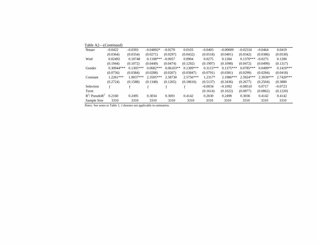
Table A2—(Continued) Nmarr –0.0422

(0.0364) –0.0393 (0.0354)

–0.04002* (0.0271)

–0.0270 (0.0297)

0.0103 (0.0432)

–0.0403 (0.0518)

–0.00009 (0.0401)

–0.02316 (0.0342)

–0.0464 (0.0386)

0.0419 (0.0530)

Wnd 0.02492 (0.1944)

0.10748 (0.1072)

0.1108***(0.0449)

–0.0057 (0.0474)

0.0904 (0.1292)

0.0275 (0.1997)

0.1284 (0.1098)

0.1370***(0.0472)

–0.0275 (0.0499)

0.1200 (0.1317)

Gender 0.30944***(0.0756)

0.1305***(0.0384)

0.0682***(0.0288)

0.06103**(0.0267)

0.1309*** (0.03847)

0.3115***(0.0791)

0.1375***(0.0381)

0.0785***(0.0299)

0.0499** (0.0284)

0.1419***(0.0418)

Constant 1.2261*** (0.2724)

1.9037***(0.1588)

2.3505***(0.1348)

2.58730 (0.1265)

2.5756*** (0.18616)

1.2317* (0.5137)

2.1986***(0.3436)

2.5924***(0.2677)

2.3939***(0.2504)

2.7420***(0.3880

Selection Term

ƒ

ƒ ƒ ƒ ƒ –0.0034 (0.1614)

–0.1092 (0.1022)

–0.08510 (0.0877)

0.0717 (0.0862)

–0.0723 (0.1220)

R2/ PseudoR2 0.2160 0.2495 0.3034 0.3691 0.4142 0.2630 0.2498 0.3036 0.4142 0.4142 Sample Size 3310 3310 3310 3310 3310 3310 3310 3310 3310 3310

Notes: See notes to Table 1; ƒ denotes not applicable in estimation.

7

Table A3

Quantile Regression Model Estimates for Private Sector, Pakistan 2001-02 Uncorrected for Selectivity Bias Corrected for Selectivity Bias

Variable 10th

Percentile 25th

Percentile 50th

Percentile 75th

Percentile 90th

Percentile 10th

Percentile 25th

Percentile 50th

Percentile 75th

Percentile 90th

Percentile Prim 0.0719

(0.0570) 0.1032***

(0.0307) 0.0636***

(0.0261) 0.0804***

(0.0244) 0.0998***

(0.0358) 0.0555

(0.0543) 0.0889***

(0.0336) 0.0427**

(0.0241) 0.0757***

(0.0281) 0.1100***

(0.0361)

Middle 0.1993*** (0.0516)

0.1765*** (0.0331)

0.1176*** (0.0275)

0.1455*** (0.0348)

0.2074*** (0.0528)

0.1693*** (0.0647)

0.1526*** (0.0447)

0.0937*** (0.0306)

0.1369*** (0.0364)

0.2248*** (0.0529)

Matric 0.2183*** (0.0542)

0.1632*** (0.0346)

0.1790*** (0.0370)

0.2160*** (0.0257)

0.2611*** (0.0424)

0.1814*** (0.0693)

0.1385*** (0.0523)

0.1433*** (0.0430)

0.1982*** (0.0373)

0.3037*** (0.0612)

Inter 0.3843*** (0.065)

0.3058*** (0.0476)

0.3145*** (0.0483)

0.31143***(0.0599)

0.4187*** (0.0701)

0.3364*** (0.0920)

0.2787*** (0.0643)

0.2564*** (0.0554)

0.2865*** (0.0716)

0.4557*** (0.0878)

Profe. 0.7413*** (0.1515)

0.8594*** (0.1424)

1.1016*** (0.1272)

1.0775*** (0.1225)

1.4365*** (0.2126)

0.6951*** (0.1729)

0.7588*** (0.1657)

1.0369*** (0.1402)

1.0730*** (0.1224)

1.4981*** (0.2133)

University 0.6175*** (0.1136)

0.6364*** (0.0744)

0.6939*** (0.0592)

0.7365*** (0.0693)

0.8728*** (0.1077)

0.5765*** (0.1149)

0.5967*** (0.0750)

0.6059*** (0.0646)

0.7112*** (0.0732)

0.9272*** (0.1078)

Pgrad

0.8514*** (0.1233)

1.0437*** (0.1451)

1.0566*** (0.0840)

1.0031*** (0.1058)

1.2283*** (0.1829)

0.7915*** (0.1793)

0.9697*** (0.1639)

0.9511*** (0.1044)

0.9846*** (0.1153)

1.2902*** (0.2024)

Train 0.0316 (0.0768)

–0.0093 (0.0407)

–0.0543 (0.0428)

0.0068 (0.06145)

0.2035*** (0.0996)

0.0121 (0.0774)

–0.0126 (0.0439)

–0.0457 (0.0404)

0.0011 (0.0600)

0.1761** (0.1035)

Age 0.0452*** (0.0117)

0.05000***(0.0072)

0.0467*** (0.0062)

0.0476*** (0.0056)

0.0410*** (0.0105)

0.0403*** (0.0127)

0.0459*** (0.0101)

0.0422*** (0.0073)

0.0431*** (0.0070)

0.0431*** (0.0107)

Continued—

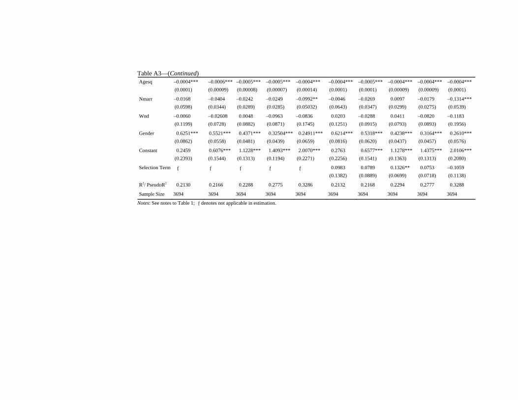
Table A3—(Continued) Agesq –0.0004***

(0.0001) –0.0006***(0.00009)

–0.0005*** (0.00008)

–0.0005*** (0.00007)

–0.0004*** (0.00014)

–0.0004*** (0.0001)

–0.0005*** (0.0001)

–0.0004*** (0.00009)

–0.0004*** (0.00009)

–0.0004*** (0.0001)

Nmarr –0.0168 (0.0598)

–0.0404 (0.0344)

–0.0242 (0.0289)

–0.0249 (0.0285)

–0.0992** (0.05032)

–0.0046 (0.0643)

–0.0269 (0.0347)

0.0097 (0.0299)

–0.0179 (0.0275)

–0.1314*** (0.0539)

Wnd –0.0060 (0.1199)

–0.02608 (0.0728)

0.0048 (0.0882)

–0.0963 (0.0871)

–0.0836 (0.1745)

0.0203 (0.1251)

–0.0288 (0.0915)

0.0411 (0.0793)

–0.0820 (0.0893)

–0.1183 (0.1956)

Gender 0.6251*** (0.0862)

0.5521*** (0.0558)

0.4371*** (0.0481)

0.32504***(0.0439)

0.24911*** (0.0659)

0.6214*** (0.0816)

0.5318*** (0.0620)

0.4238*** (0.0437)

0.3164*** (0.0457)

0.2610*** (0.0576)

Constant 0.2459 (0.2393)

0.6076*** (0.1544)

1.1228*** (0.1313)

1.4093*** (0.1194)

2.0070*** (0.2271)

0.2763 (0.2256)

0.6577*** (0.1541)

1.1278*** (0.1363)

1.4375*** (0.1313)

2.0106*** (0.2080)

Selection Term ƒ ƒ ƒ ƒ ƒ 0.0983 (0.1382)

0.0789 (0.0889)

0.1326** (0.0699)

0.0753 (0.0718)

–0.1059 (0.1138)

R2/ PseudoR2 0.2130 0.2166 0.2288 0.2775 0.3286 0.2132 0.2168 0.2294 0.2777 0.3288

Sample Size 3694 3694 3694 3694 3694 3694 3694 3694 3694 3694


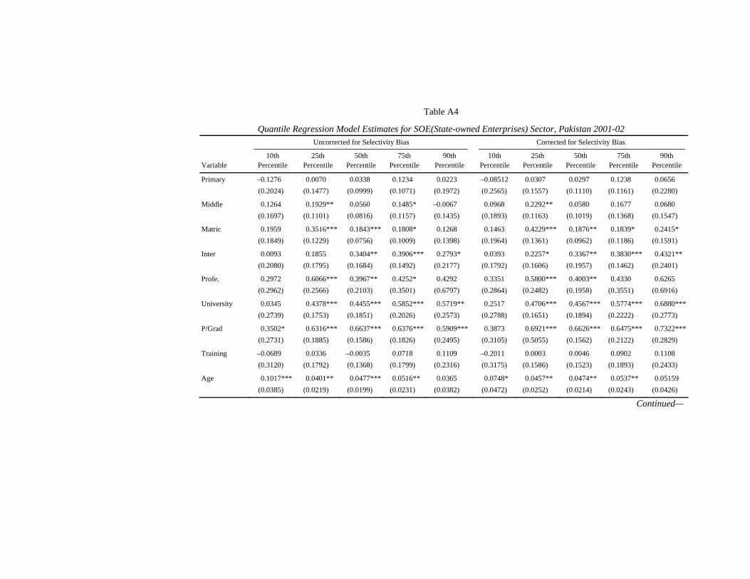
Table A4

Quantile Regression Model Estimates for SOE(State-owned Enterprises) Sector, Pakistan 2001-02 Uncorrected for Selectivity Bias Corrected for Selectivity Bias

Variable 10th

Percentile 25th

Percentile 50th

Percentile 75th

Percentile 90th

Percentile 10th

Percentile 25th

Percentile 50th

Percentile 75th

Percentile 90th

Percentile

Primary –0.1276 (0.2024)

0.0070 (0.1477)

0.0338 (0.0999)

0.1234 (0.1071)

0.0223 (0.1972)

–0.08512 (0.2565)

0.0307 (0.1557)

0.0297 (0.1110)

0.1238 (0.1161)

0.0656 (0.2280)

Middle 0.1264 (0.1697)

0.1929** (0.1101)

0.0560 (0.0816)

0.1485* (0.1157)

–0.0067 (0.1435)

0.0968 (0.1893)

0.2292** (0.1163)

0.0580 (0.1019)

0.1677 (0.1368)

0.0680 (0.1547)

Matric 0.1959 (0.1849)

0.3516***(0.1229)

0.1843***(0.0756)

0.1808* (0.1009)

0.1268 (0.1398)

0.1463 (0.1964)

0.4229***(0.1361)

0.1876** (0.0962)

0.1839* (0.1186)

0.2415* (0.1591)

Inter 0.0093 (0.2080)

0.1855 (0.1795)

0.3404** (0.1684)

0.3906***(0.1492)

0.2793* (0.2177)

0.0393 (0.1792)

0.2257* (0.1606)

0.3367** (0.1957)

0.3830***(0.1462)

0.4321** (0.2401)

Profe. 0.2972 (0.2962)

0.6066***(0.2566)

0.3967** (0.2103)

0.4252* (0.3501)

0.4292 (0.6797)

0.3351 (0.2864)

0.5800***(0.2482)

0.4003** (0.1958)

0.4330 (0.3551)

0.6265 (0.6916)

University 0.0345 (0.2739)

0.4378***(0.1753)

0.4455***(0.1851)

0.5852***(0.2026)

0.5719** (0.2573)

0.2517 (0.2788)

0.4706***(0.1651)

0.4567***(0.1894)

0.5774***(0.2222)

0.6880***(0.2773)

P/Grad 0.3502* (0.2731)

0.6316***(0.1885)

0.6637***(0.1586)

0.6376***(0.1826)

0.5909*** (0.2495)

0.3873 (0.3105)

0.6921***(0.5055)

0.6626***(0.1562)

0.6475***(0.2122)

0.7322***(0.2829)

Training –0.0689 (0.3120)

0.0336 (0.1792)

–0.0035 (0.1368)

0.0718 (0.1799)

0.1109 (0.2316)

–0.2011 (0.3175)

0.0003 (0.1586)

0.0046 (0.1523)

0.0902 (0.1893)

0.1108 (0.2433)

Age 0.1017*** (0.0385)

0.0401** (0.0219)

0.0477***(0.0199)

0.0516** (0.0231)

0.0365 (0.0382)

0.0748* (0.0472)

0.0457** (0.0252)

0.0474** (0.0214)

0.0537** (0.0243)

0.05159 (0.0426)

Continued—

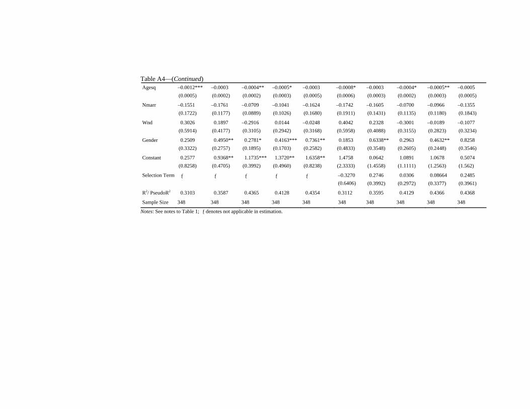
Table A4—(Continued) Agesq –0.0012***

(0.0005) –0.0003 (0.0002)

–0.0004** (0.0002)

–0.0005* (0.0003)

–0.0003 (0.0005)

–0.0008* (0.0006)

–0.0003 (0.0003)

–0.0004* (0.0002)

–0.0005** (0.0003)

–0.0005 (0.0005)

Nmarr –0.1551 (0.1722)

–0.1761 (0.1177)

–0.0709 (0.0889)

–0.1041 (0.1026)

–0.1624 (0.1680)

–0.1742 (0.1911)

–0.1605 (0.1431)

–0.0700 (0.1135)

–0.0966 (0.1180)

–0.1355 (0.1843)

Wnd 0.3026 (0.5914)

0.1897 (0.4177)

–0.2916 (0.3105)

0.0144 (0.2942)

–0.0248 (0.3168)

0.4042 (0.5958)

0.2328 (0.4088)

–0.3001 (0.3155)

–0.0189 (0.2823)

–0.1077 (0.3234)

Gender 0.2509 (0.3322)

0.4950** (0.2757)

0.2781* (0.1895)

0.4163*** (0.1703)

0.7361** (0.2582)

0.1853 (0.4833)

0.6338** (0.3548)

0.2963 (0.2605)

0.4632** (0.2448)

0.8258 (0.3546)

Constant 0.2577 (0.8258)

0.9368** (0.4705)

1.1735*** (0.3992)

1.3720** (0.4960)

1.6358** (0.8238)

1.4758 (2.3333)

0.0642 (1.4558)

1.0891 (1.1111)

1.0678 (1.2563)

0.5074 (1.562)

Selection Term ƒ ƒ ƒ ƒ ƒ –0.3270 (0.6406)

0.2746 (0.3992)

0.0306 (0.2972)

0.08664 (0.3377)

0.2485 (0.3961)

R2/ PseudoR2 0.3103 0.3587 0.4365 0.4128 0.4354 0.3112 0.3595 0.4129 0.4366 0.4368

Sample Size 348 348 348 348 348 348 348 348 348 348



Table A5

OLS Estimates for Public, Private, and SOE Sectors, Pakistan 2001-02 Without Correction for

Selectivity Bias With Correction for

Selectivity Bias Variable Public Private SOE Public Private SOE Prim 0.06145**

(0.0292) 0.0946***

(0.0250) 0.01117

(0.1141) 0.0607**

(0.0351) 0.0849***

(0.0268) 0.0107

(0.1132)

Middle 0.0906*** (0.0276)

0.1829*** (0.0296)

0.04624 (0.0881)

0.0895** (0.0414)

0.1676*** (0.0339)

0.0416 (0.0939)

Matric 0.21640*** (0.0268)

0.2142*** (0.029)

0.1738** (0.0914)

0.2149*** (0.0523)

0.1911*** (0.0385)

0.1688** (0.0972)

Inter 0.32102*** (0.0323)

0.3614*** (0.0411)

0.2404* (0.1363)

0.3191*** (0.0631)

0.3295*** (0.0525)

0.2384** (0.1373)

Profe. 0.68430*** (0.0769)

1.0585*** (0.1031)

0.5095** (0.2192)

0.6827*** (0.0917)

1.0319*** (0.107)

0.5034** (0.2209)

University 0.44876*** (0.0352)

0.7135*** (0.0506)

0.4578** (0.1758)

0.4470*** (0.0637)

0.6815*** (0.0604)

0.454*** (0.1769)

Pgrad 0.64456*** (0.0434)

1.0709*** (0.0819)

0.5756*** (0.1515)

0.6425*** (0.0764)

1.0204*** (0.097)

0.5701*** (0.1559)

Train 0.04767* (0.03715)

0.0233 (0.0478)

0.0213 (0.1575)

0.0475 (0.038)

0.0184 (0.047)

0.0194 (0.1647)

Age 0.02016*** (0.0065)

0.0445*** (0.0062)

0.0410** (0.0217)

0.0198** (0.0107)

0.0414*** (0.007)

0.0403** (0.0229)

Agesq –0.00012* (0.00008)

–0.0004*** (0.00008)

–0.00034 (0.0002)

–0.0001 (0.0001)

–0.0004*** (0.00008)

–0.0003 (0.00030)

Nmarr –0.0509* (0.0293)

–0.0543** (0.0303)

–0.1789** (0.0974)

–0.0571* (0.0364)

–0.0424* (0.0323)

–0.1816** (0.1076)

Wnd 0.08029* (0.0615)

–0.0325 (0.0744)

0.04133 (0.2745)

0.0809 (0.0652)

–0.0163 (0.0756)

0.0484 (0.2927)

Gender 0.14957*** (0.0293)

0.42797***(0.0431)

0.3535*** (0.1341)

0.1498*** (0.0304)

0.4240*** (0.0433)

0.3404** (0.1953)

Constant 2.10676*** (0.1299)

1.0927*** (0.1329)

1.4248*** (0.41070)

2.1151*** (0.2846)

1.1028*** (0.1337)

1.5129* (1.0240)

Selection Term ƒ ƒ ƒ –0.0030 (0.0941)

0.0683 (0.0664)

–0.0252 (0.2696)

R-squared

0.4609 0.3948 0.5465 0.4609 0.3949 0.5465

Sample Size 3310 3948 348 3310 3948 348



Table A6

Rates of Return to Educational Qualifications in Pakistan Public Sector Private Sector Differential Primary 0.0121***

(0.0070) 0.0170*** (0.0054)

–0.0049 (0.0088)

Middle 0.0100 (0.0112)

0.0275*** (0.0104)

–0.0175 (0.0153)

Matriculation 0.0627*** (0.0261)

0.0118 (0.0172)

0.0509 (0.0312)

Intermediate 0.0521*** (0.0129)

0.0693*** (0.0210)

–0.0172 (0.0246)

Professional 0.0723*** (0.0143)

0.1405*** (0.0208)

–0.0682*** (0.0252)

Undergraduate 0.0639*** (0.0138)

0.1760*** (0.0267)

–0.1121*** (0.0300)

Postgraduate 0.0977*** (0.0194)

0.1694*** (0.0429)

–0.0717 (0.0471)

Notes: (a) The rates of return are computed using the estimates from the mean regression corrected for selectivity bias.

(b) Standard errors are reported in parentheses. (c) ***, **, * denote statistical significance at the 1 percent, 5 percent and 10 percent level

respectively using two-tailed tests. (d) In computing the rates of return we assumed primary=5 years; middle=3 years;

matriculation=2 years; intermediate=2 years; professional=5; undergraduate=2 years; and postgraduate = 2 years.

Table A7

Decomposition of Sectoral Wage Gaps at Selected Quantiles: SOE/Private Due to

Treatment Due to


Terms Residuals Total SOE/Privateθ=0.10 0.3398***

(0.0415) 0.2298***

(0.0256) Not applicable 0.0366 0.6063

1.1358 (1.3547)

0.1392 (0.1878)

–0.7028 0.0342 0.6063

SOE/Private θ=0.25 0.2999*** (0.0691)

–0.3785 (0.3374)


–0.2699 (0.9420)

–0.3964 (0.3311)

0.5125 0.6942 0.5404

SOE/Private θ=0.5 0.2892*** (0.0496)

0.8486*** (0.3514)


0.2936 (0.6256)

0.8501 (0.3684)

–0.0123 –0.5223 0.5891

SOE/Private θ=0.75 0.2586*** (0.0526)

–0.3559 (0.3465)


0.11949 (0.7122)

–0.3774 (0.3569)

0.1214 0.8522 0.7157

SOE/Private θ=0.9 0.1735** (0.0999)

0.61006*** (0.1224)


–0.4252 (0.7774)

0.6576*** (0.1249)

0.54378 –0.0005 0.7755

Notes: See notes to Table 3.


Table A8

Decomposition of Sectoral Wage Gaps at Selected Quantiles: Public/SOE Due to

Treatment Due to


Terms Residuals Total Public/SOEθ=0.10 0.2393***

(0.0665) 0.0040

(0.0288) Not applicable 0.04649 0.2898

–0.4124 (1.2983)

0.0022 (0.0784)

0.6615 0.0386 0.2898

Public/SOE θ=0.25 0.37846 (0.3814)

0.4443*** (0.1234)


1.2687 (1.0287)

0.2552 (0.2367)

–0.6229 –0.6995 0.2016

Public/SOE θ=0.5 –0.5377* (0.36708)

0.08799** (0.0383)


–0.4979 (0.6301)

0.0926*** (0.0380)

–0.1129 0.5815 0.0633

Public/SOE θ=0.75 0.4922 (0.40920)

0.2415*** (0.1054)

Not applicable –0.8516 –0.1179

0.5405 (0.8832)

0.3607** (0.1739)

–0.1267 –0.8925 -0.1179

Public/SOE θ=0.9 –0.1559* (0.1204)

–0.1673* (0.1182)

Not applicable 0.4727 –0.1495

0.3653 (0.7586)

–0.1193 (0.1732)

–0.5048 –0.4083 –0.1495

Notes: See notes to Table 3.

REFERENCES

Adamchik, V. A., and A. S. Bedi (2000) Wage Differentials between the Public and Private Sectors: Evidence from an Economy in Transition. Labour Economics 7, 203–224.

Ajwad, I. M., and P. Kurukulasuriya (2002) Ethnic and Gender Wage Disparities in Sri Lanka. World Bank, Washington, D. C. (World Bank Policy Research Working Paper No. 2859.)

Albrecht, J., A. Björklund, and S. Vroman (2003) Is There a Class Ceiling in Sweden. Journal of Labour Economics 21, 145–177.

Al-Sammarai, S., and B. Reilly (2005) Education, Employment and Earnings of Secondary School-Leavers in Tanzania: Evidence from a Tracer Study. Poverty Research Unit at Sussex. Department of Economics, University of Sussex, Brighton, United Kingdom. (Working Paper No. 31.)

Andrews, D., and M. Schafgans (1998) Semi-parametric Estimation of the Intercept of a Sample Selection Model. Review of Economics and Statistics 65, 497–517.


Arbache, J. S., A. Dickerson, and F. Green (2004) Trade Liberalisation and Wages in Developing Countries. The Economic Journal 114:493, F73–F96.

Blackaby, D., P. Murphy, and N. O’Leary (1999) The Payment of Public Sector Workers in the UK: Reconciliation with North-American Findings. Economics Letters 65, 239–243.

Blank, R. (1994) Public Sector Growth and Labour Market Flexibility: The US versus the UK. In R. Blank (ed.) Social Protection versus Economic Flexibility: Is there a Trade-off? NBER-CLM Series.

Blinder, A. S. (1973) Wage Discrimination: Reduced Form and Structural Variables. Journal of Human Resources 8, 436–455.

Boudarbat, B. (2004) Employment Sector Choice in a Developing Labour Market. Department of Economics, University of British Columbia. (Mimeographed.)

Brownstone, D., and R. Valletta (2001) The Bootsrap and Multiple Imputations: Harnessing Increased Computing Power for Improved Statistical Tests. Journal of Economic Perspectives 15:4, 129–141.

Buchinsky, M. (1999) The Dynamics of Changes in the Female Wage Distribution in the USA: A Quantile Regression Approach. Journal of Applied Econometrics 13, 1–30.

Chamberlain, G. (1994) Quantile Regression, Censoring and the Structure of Wages In C. Sims and J. J. Laffont (eds.) Proceedings of the Sixth World Congress of the Econometrics Society. New York: Cambridge University Press. 171–209.

Deaton, A. (1997) The Analysis of Household Surveys: A Microeconometric Approach to Development Policy. John Hopkins University Press.

DiNardo, J., N. Fortin, and T. Lemieux (1996) Labour Market Institutions and the Distribution of Wages, 1973–1992: A Semi-parametric Approach. Econometrica 64, 1001–1044.

Disney, R., and A. Gosling (1998) Does it Pay to Work in the Public Sector? Fiscal Studies 19, 347–374.

Donald, S., D. Green, and Paarsch (2000) Differences in Wage Distributions Between Canada and the United States: An Application of a Flexible Estimator of Distribution Functions in the Presence of Covariates. Review of Economics Studies 67, 609–633.

Dustmann, C., and A. Van Soest (1998) Public and Private Sector Wages of Male Workers in Germany. European Economic Review 42, 1417–1441.

Falaris, E. M. (2003) A Quantile Regression Analysis of Wages in Panama. Department of Economics, University of Delaware. (Mimeographed.)

Filer, R., and J. Hanousek (2002) Research Data from Transition Economies. Journal of Economic Perspectives 16, 225 – 240.

Fitzenberger, B. (2003) Gender Wage Differentials Across Quantiles, Accounting for Sample Selection. University of Mannheim, Germany. (Mimeographed.)


Fortin, N. M., and T. Lemieux (1998) Rank Regressions, Wage Distributions and the Gender Pay Gap. Journal of Human Resources 33, 610–643.

Freeman, Richard B. (1981) The Effect of Unionism on Fringe Benefits. Industrial and Labour Relation Review 34, 489– 510.

Gardeazabal, J., and A. Ugidos (2005) Measuring the Wage Distribution Gender Gap at Quantiles. Journal of Population Economics 18, 65–179.

Gregory, R. G., and J. Borland (1999) Recent Developments in Public Sector Labour Markets. (Chapter 53.) In O. Ashenfelter and D. Card (ed.) Handbook of Labour Economics. Volume 3C. Elsevier Science B.V.

Gyourko, J., and J. Tracy (1988) An Analysis of Public- and Private-Sector Wages Allowing for both Endogenous Choice of Government and Unions. Journal of Labor Economics 6, 229–253.

Heckman, J. (1979) Sample Selection Bias as a Specification Error. Econometrica 47, 153–161.

Heckman, J. (1990) Varieties of Selection Bias. American Economic Review 80, 1121–1149.

Huber, P. J. (1967) The Behaviour of Maximum Likelihood Estimates under Non-standard Conditions. In Proceedings of the Fifth Berkeley Symposium on Mathematical Statistics and Probability. Berkeley, CA: University of California Press. 1, 221 – 223.

Ichniowski, Casey (1980) Economic Effect of Firefighter’s Union. Industrial and Labour Relation Review 33, 198– 211.

Jovičić, M., Nojković, A., and A. Paranos (2000) Labour Force Survey Data on Wages and Earnings in the Private and Social Sectors in FR Yugoslavia. Paper delivered to the 10th Conference of the IAFEP, University of Trento.

Koenker, R. (2005) Quantile Regression. Econometric Society. Cambridge University Press (Monographs No. 38.)

Koenker, R., and G. Bassett (1978) Regression Quantiles. Econometrica 46, 33–50.

Krstić, G., B. Reilly, and M-C Tabet (2004) The Private Sector Wage Premium in Serbia (1995–2000): A Quantile Regression Approach. Ekonomska Misao 38, 1–27.

Lee, L. (1983) Generalised Models with Selectivity. Econometrica 51, 507–512. Lindauer, D., and R. H. Sabot (1983) The Public-Private Wage Differential in a Poor

Urban Economy. Journal of Development Economics 12: 3, 137–152. Lokshin, M., and B. Jovanovic (2001) Public-private Sector Employment Choice and

Wage Differentials in Yugoslavia. World Bank, Washington, D. C. (Mimeographed.)

Lokshin, M., and B. Jovanovic (2002) Wage Differentials between the State and the Private Sector in Moscow. World Bank, Washington, D. C. (Mimeographed).


Lucifora, C., and D. Meurs (2004) The Public Sector Pay Gap in France, Great Britain and Italy. (IZA Discussion Paper No. 1024.)

Machado, J., and J. Mata (2000) Counterfactual Decomposition of Changes in Wage Distributions Using Quantile Regression Models. Department of Economics, Universidade de Lisboa, Portugal. (Mimeographed.)

Moulton, B. R. (1990) A Re-examination of the Federal-Private Wage Differential in the United States. Journal of Labour Economics 8, 270–293.

Mueller, R. (1998) Public-Private Sector Wage Differentials in Canada: Evidence from Quantile Regression. Economics Letters 60, 229–235.

Nasir, Z. M. (2000) Earnings Differential between Public and Private Sectors in Pakistan. The Pakistan Development Review 39: 2, 111–130.

Neuman, S., and R. L. Oaxaca (2004), Wage Decompositions with Selectivity-Corrected Wage Equations: A Methodological Note. Journal of Economic Inequality 2, 3–10.

Newell, A. T., and M. Socha (1998) Wage Distribution in Poland: The Role of Privatisation and International Trade, 1992–1996. Economics of Transition 6, 47–65.

Newey, W. K. (1999) Two Step Series Estimation of Sample Selection Models. MIT. (Mimeographed.)

Oaxaca, R. L. (1973) Male-Female Wage Differentials in Urban Labour Markets. International Economic Review 14, 693–709.

Panizza, U. (2000) The Public Sector Premium and the Gender Gap in Latin America: Evidence for the 1980s and 1990s. Inter-American Development Bank. (Research Department Working Paper No. 431.)

Poterba, R., and K. Reuben (1994) The Distribution of the Public Sector Wage Premia: New Evidence Using Quantile Regression Methods (NBER Working Paper No. 4734.)

Rees, H., and A. Shah (1995) Public-Private Sector Wage Differentials in the UK. The Manchester School 63, 52–68.

Reimers, C. (1983) Labour Market Discrimination Against Hispanic and Black Men. Review of Economics and Statistics 65, 570–579.

Skyt-Nielsen, H., and M. Rosholm (2001) The Public-Private Sector Wage Gap in Zambia in the 1990s: A Quantile Regression Approach. Empirical Economics 26, 169–182.

Terrell, K. (1993) Public-Private Wage Differentials in Haiti: Do Public Servants Earn a Rent? Journal of Development Economics 42, 293–314.

Van der Gaag, J., and W. Vijerberg (1988) A Switching Regression Model for Wage Determinants in the Public and Private Sectors of a Developing Country. Review of Economics and Statistics 70, 244–252.


Van der Gaag, J., J. M. Stelcner, and W. Vijerberg (1989) Wage Differentials and Moonlighting by Civil Servants: Evidence from Cote d'Ivoire and Peru. World Bank Economic Review 3, 67–95.

Van Ophem, H. (1993) A Modified Switching Regression Model for Earnings Differentials between Pubic and Private Sectors in the Netherlands. Review of Economics and Statistics 75, 215–224.

The Public and Private Sector Pay Gap in Pakistan - CiteSeerX

Documents

Transcript of The Public and Private Sector Pay Gap in Pakistan - CiteSeerX