arX

iv:h

ep-p

h/97

0929

3v1

9 S

ep 1

997

The Proton Spin and Flavor Structure in the

Chiral Quark Model

Ling-Fong Li∗ and T. P. Cheng†∗Department of Physics, Carnegie Mellon University

Pittsburgh, PA 15213, USA

†Department of Physics and Astronomy, University of Missouri

St. Louis, MO 63121, USA

Schladming Lectures (March 1997)

Abstract

After a pedagogical review of the simple constituent quark model

and deep inelastic sum rules, we describe how a quark sea as produced

by the emission of internal Goldstone bosons by the valence quarks can

account for the observed features of proton spin and flavor structures.

Some issues concerning the strange quark content of the nucleon are

also discussed.

Contents

1 Strong Interaction Symmetries and the Quark Model 31.1 Current quark mass ratios as deduced from pseudoscalar me-

son masses . . . . . . . . . . . . . . . . . . . . . . . . . . . . . 31.1.1 Gell-Mann-Okubo mass relation and the strange to

non-strange quark mass ratio . . . . . . . . . . . . . . 41.1.2 Isospin breaking by the strong interaction & themu/md

ratio . . . . . . . . . . . . . . . . . . . . . . . . . . . . 51.2 Quark masses from fitting baryon masses . . . . . . . . . . . . 61.3 The constituent quark model . . . . . . . . . . . . . . . . . . . 9

1.3.1 Spin-dependent contributions to baryon masses . . . . 9

1

1.3.2 Spin and magnetic moments of the baryon . . . . . . . 121.3.3 sQM lacks a quark sea . . . . . . . . . . . . . . . . . . 17

1.4 The OZI rule . . . . . . . . . . . . . . . . . . . . . . . . . . . 191.4.1 The OZI rule for mesons . . . . . . . . . . . . . . . . . 191.4.2 The OZI rule and the strange quark content of the

nucleon . . . . . . . . . . . . . . . . . . . . . . . . . . 21

2 Deep Inelastic Scatterings 222.1 Polarized lepton-nucleon scatterings . . . . . . . . . . . . . . . 22

2.1.1 Kinematics and Bjorken scaling . . . . . . . . . . . . . 232.1.2 Inclusive sum rules via operator product expansion . . 242.1.3 The parton model approach . . . . . . . . . . . . . . . 282.1.4 Axial vector current and the axial anomaly . . . . . . . 302.1.5 Semi-inclusive polarized DIS . . . . . . . . . . . . . . . 312.1.6 Baryon magnetic moments . . . . . . . . . . . . . . . . 32

2.2 DIS on proton vs neutron targets . . . . . . . . . . . . . . . . 332.2.1 Lepton-nucleon scatterings . . . . . . . . . . . . . . . . 332.2.2 Drell-Yan processes . . . . . . . . . . . . . . . . . . . . 34

3 The Proton Spin-Flavor Structure in the Chiral Quark Model 363.1 The naive quark sea . . . . . . . . . . . . . . . . . . . . . . . 363.2 The chiral quark idea of Georgi and Manohar . . . . . . . . . 383.3 Flavor-spin structure of the nucleon . . . . . . . . . . . . . . . 41

3.3.1 Chiral quark model with an octet of Goldstone bosons 413.3.2 Chiral quark model with a nonet of Goldstone bosons . 44

3.4 Strange quark content of the nucleon . . . . . . . . . . . . . . 493.4.1 The scalar channel . . . . . . . . . . . . . . . . . . . . 493.4.2 The axial-vector channel . . . . . . . . . . . . . . . . . 503.4.3 The pseudoscalar channel . . . . . . . . . . . . . . . . 523.4.4 The vector channel . . . . . . . . . . . . . . . . . . . . 53

3.5 Discussion . . . . . . . . . . . . . . . . . . . . . . . . . . . . . 54

2

We shall first recall the contrasting concepts of current quarks vs con-stituent quarks. In the first Section we also briefly review the successes andinadequacies of the simple constituent quark model (sQM) which attemptsto describe the properties of light hadrons as a composite systems of u, d, ands valence quarks. Some of the more prominent features, gleaned from themass and spin systematics, are discussed. In the Sec. 2 we shall provide apedagogical review of the deep inelastic sum rules that can be derived by wayof operator product expansion and/or the simple parton model. We show inparticular how some the sum rules in the second category can be interpretedas giving information of the nucleon quark sea. In the remainder of theselectures we shall show that the account of the quark sea as given by the chiralquark model is in broad agreement with the experimental observation.

1 Strong Interaction Symmetries and the Quark

Model

In the approximation of neglecting the light quark masses, the QCD La-grangian has the global SU (3)L×SU (3)R symmetry. Namely, it is invariantunder independent SU (3) transformation of the three left-handed and right-handed light quark fields. This symmetry is realized in the Nambu-Goldstonemode with the ground state being symmetric only with respect to the vectorSU (3)L+R transformations. This gives rise to an octet of Goldstone bosons,which are identified with the low lying pseudoscalar mesons (π, K, η) . Fora pedagogical review see, for example, ref.[1].

1.1 Current quark mass ratios as deduced from pseu-

doscalar meson masses

The light current quark masses are the chiral symmetry breaking parametersof the QCD Lagrangian. Their relative magnitude can be deduced from thesoft meson theorems for the pseudoscalar meson masses.

The matrix element of an axial vector current operator Aaµ taken between

the vacuum and one meson φb state (with momentum kµ) defines the decayconstant fa as ⟨

0∣∣∣Aaµ

∣∣∣ φb (k)⟩

= ikµfaδab

3

where the SU(3) indices a, b...range from 1, 2, ....8. This means that the di-vergence of the axial vector current has matrix element of

⟨0∣∣∣∂µAaµ

∣∣∣φb (k)⟩

= m2afaδab, (1)

If the axial divergences are good interpolating fields for the pseudoscalarmesons, we have the result of PCAC:

∂µAaµ = m2afaφ

a. (2)

Using PCAC and the reduction formula we can derive a soft-meson theoremfor the pseudoscalar meson masses:

m2af

2aδab = −i

∫d4xe−ik·x

⟨0∣∣∣δ (x0)

[Ab0 (x) , ∂µAaµ (0)

]∣∣∣ 0⟩

= −⟨0∣∣∣[Q5b,

[Q5a,H (0)

]]∣∣∣ 0⟩

(3)

where the axial charge is related to the time component of the axial vectorcurrent as Q5a =

∫d3xAa0 (x) .

If we neglect the electromagnetic radiative correction, only the quarkmasses,

Hm = muuu+mddd+msss, (4)

break the chiral symmetry. Hence only such terms are relevant in the com-putation of the above commutators. [In actual computation it is simpler ifone takes Hm and Q5a to be 3 × 3 matrices and compute directly the anti-commutator in

[q λ

a

2γ0γ5q, qλ

bq]

= −12qλa, λb

γ5q.] In this way we obtain:

f 2πm

2π =

1

2(mu +md)

⟨0∣∣∣(uu+ dd

)∣∣∣ 0⟩

f 2Km

2K =

1

2(mu +ms) 〈0 |(uu+ ss)| 0〉 (5)

f 2ηm

2η =

1

6(mu +md)

⟨0∣∣∣(uu+ dd

)∣∣∣ 0⟩

+4

3ms 〈0 |ss| 0〉 .

1.1.1 Gell-Mann-Okubo mass relation and the strange to non-strange quark mass ratio

Since the flavor SU(3) symmetry is not spontaneously broken,

〈0 |uu| 0〉 =⟨0∣∣∣dd∣∣∣ 0⟩

= 〈0 |ss| 0〉 ≡ µ3 (6)

4

and fπ = fK = fη ≡ f ; Eq.(5) is simplified to

m2π = 2mn

µ3

f 2

m2K = (mn +ms)

µ3

f 2

m2η =

2

3(mn + 2ms)

µ3

f 2(7)

where we have made the approximation of mu ≃ md ≡ mn. From this, wecan deduce the Gell-Mann-Okubo mass relation for the 0− mesons:

3m2η = 4m2

K −m2π, (8)

as well as the strange to nonstrange quark mass ratio [2]:

mn

ms=mu +md

2ms=

m2π

2m2K −m2

π

≃ 1

25. (9)

1.1.2 Isospin breaking by the strong interaction & the mu/md ratio

In order to study the ratio of mu/md, we need to include the electromagneticradiative contribution to the masses. The effective Hamiltonian due to virtualphoton exchange is given by

Hγ = e2∫d4xT

(Jemµ (x) Jemν (0)

)Dµν (x) (10)

where Dµν (x) is the photon propagator. Thus, beside the contribution fromHm, we also have the additional term on the RHS of eqn.(3):

σabγ =⟨0∣∣∣[Q5b,

[Q5a,Hγ

]]∣∣∣ 0⟩

(11)

Now we make the observation (Dashen’s theorem[3]) : For the electricallyneutral mesons, we have [Q5a,Hγ] = 0, which leads to

σγ(π0)

= σγ(K0)

= σγ (η) = 0. (12)

On the other hand, Jemµ is invariant (i.e. U-spin symmetric) under the in-terchange d ↔ s, which transforms charged mesons π+ and K+ into eachother:

σγ(π+)

= σγ(K+

)≡ µ3

γ (13)

5

Consequently, we obtain the generalization of (7) as

f 2m2(π+)

= (mu +md)µ3 + µ3

γ

f 2m2(π0)

= (mu +md)µ3

f 2m2(K+

)= (mu +ms)µ

3 + µ3γ (14)

f 2m2(K0)

= (md +ms)µ3

f 2m2 (η) =1

3(mu +md + 4ms)µ

3.

From this we can obtain the current quark mass ratios:

m2 (K0) + [m2 (K+) −m2 (π+)]

m2 (K0) − [m2 (K+) −m2 (π+)]=

ms

md

≃ 20.1 (15)

m2 (K0) − [m2 (K+) −m2 (π+)]

[2m2 (π0) −m2 (K0)] + [m2 (K+) −m2 (π+)]=

md

mu≃ 1.8 (16)

If we assume, for example, ms ≃ 190MeV, these ratios yield:

mu ≃ 5.3MeV ms ≃ 9.5MeV or mn = 7.4MeV, (17)

which are indeed very small on the intrinsic scale of QCD. This explains whythe chiral SU(2) and isospin symmetries are such good approximations of thestrong interaction.

1.2 Quark masses from fitting baryon masses

For the baryon mass we need to study the matrix elements 〈B |H|B〉 . Theflavor SU (3) symmetry breaking being given by the quark masses (4), weneed to evaluate the matrix elements of the quark scalar densities ua betweenbaryon states :

Hm = muuu+mddd+msss

= m0u0 +m3u3 +m8u8

withm0 = 1

3(mu +md +ms) u0 = uu+ dd+ ss

m3 = 12(mu −md) u3 = uu− dd

m8 = 16(mu +md − 2ms) u8 = uu+ dd− 2ss

(18)

6

where, instead of the standard ua = qλaq (λa being the familiar Gell-Mannmatrices), we have used, for our purpose, the more convenient definitionsof scalar densities by moving some numerical factors into the quark masscombinations m0,3,8.

We shall first concentrate on the low lying baryon octet which, being theadjoint representation of SU (3) , can be written as a 3 × 3 matrix

B =

√12Σ0 +

√16Λ Σ+ p

Σ− −√

12Σ0 +

√16Λ n

Ξ− Ξ0√

23Λ

. (19)

The octet scalar densities ua can be related to two parameters (Wigner-Eckarttheorem):

〈B |ua|B〉 = α tr(B†uaB

)+ β tr

(B†Bua

)

where ua is the scalar density expressed as a 3 × 3 matrix in the quarkflavor space. The linear combinations (α± β) /2 are the familiar D and Fcoefficients. For example, we can easily compute:

〈p |u8| p〉 = α− 2β = (3F −D)mass (20)

〈p |u3| p〉 = α = (F +D)mass . (21)

In this way the baryon masses with their electromagnetic self-energy sub-tracted (as denoted by the baryon names) can be expressed in terms of threeparameters

p = M0 + (α− 2β)m8 + αm3 (22)

n = M0 + (α− 2β)m8 − αm3

Σ+ = M0 + (α + β)m8 + (α− β)m3

Σ0 = M0 + (α + β)m8

Σ− = M0 + (α + β)m8 − (α− β)m3

Ξ− = M0 + (β − 2α)m8 + βm3

Ξ0 = M0 + (β − 2α)m8 − βm3

Λ = M0 − (α+ β)m8

We have 8 baryon masses and three unknown parameters M0, α and β —hence 5 relations, one of them should yield quark mass ratio m8/m3.

7

• The (“improved”) Gell-Mann-Okubo mass relation

n+ Ξ− =1

2

(3Λ + 2Σ+ − Σ0

)(23)

• The Coleman-Glashow (U-spin) relation

Ξ− − Ξ0 = (p− n) +(Σ− − Σ+

)(24)

• Absence of isospin I = 2 correction (i.e. u3 being a member of I = 1):

Σ− + Σ+ − 2Σ0 = 0 (25)

• The hybrid relation:

p− n

Σ− − Ξ−=

Ξ− − Ξ0

Σ+ − p(26)

It should not be surprising that we have a relation relating SU (2)breakings to SU (3) breakings, since u3 and u8 belong to the sameoctet representation. Recall that here the electromagnetic contribu-tion must be subtracted from our masses (sometimes called the tadpolemasses). Since there is no Dashen theorem for the electromagnetic con-tributions to baryon masses, we must resort to detailed (& less reliable)model calculations. We quote one such result[4] for the electromagneticcontributions (∆M)γ :

p− n = (p− n)obs − (p− n)γ ≃ −1.3 − 1.1 ≃ −2.4MeV

Ξ− − Ξ0 =(Ξ− − Ξ0

)obs

−(Ξ− − Ξ0

)γ≃ 6.4 − 1.3 ≃ 5.1MeV

which yields ≃ 0.02 on both sides of Eqn.(26).

• Both sides of Eq.(26) are related to the quark mass ratio 2m3/ (3m8 −m3) . Thusthe above result leads to

(mu −md

md −ms

)

B

≃ 0.02 (27)

which is compatible with the current quark ratio deduced from pseu-doscalar meson masses Eqs.(15) and (16):

(mu −md

md −ms

)

ps

≃1

1.8− 1

1 − 20.1≃ 0.023. (28)

8

1.3 The constituent quark model

1.3.1 Spin-dependent contributions to baryon masses

The sQM which attempts to describe the properties of light hadrons as acomposite systems of u, d, and s valence quarks. The mass relations derivedabove may be interpreted simply as reflecting the hadrons masses as sum ofthe corresponding valence quark masses. For a general baryon, we have

B = M0 +M1 +M2 +M3 (29)

where M0 is some SU (3) symmetric binding contribution. M1,2,3 are the con-stituent masses of the three valence quarks. We shall ignore isospin breakingeffects: Mu = Md ≡Mn, and write the octet baryon masses as,

N = M0 + 3Mn (30)

Λ = M0 + 2Mn +Ms

Σ = M0 + 2Mn +Ms

Ξ = M0 +Mn + 2Ms,

and the decuplet baryon masses as,

∆ = M0 + 3Mn (31)

Σ∗ = M0 + 2Mn +Ms

Ξ∗ = M0 +Mn + 2Ms

Ω = M0 + 3Ms.

While it reproduces the GMO mass relations respectively, for the octet:

N + Ξ =1

2(3Λ + Σ), (32)

and for the decuplet (the equal-spacing rule):

∆ − Σ∗ = Σ∗ − Ξ∗ = Ξ∗ − Ω, (33)

it also leads to a phenomenologically incorrect result of Λ = Σ (reflectingtheir identical quark contents). Similarly, such a naive picture would lead usto expect that the N, Σ, Ξ baryons having comparable masses as ∆, Σ∗, Ξ∗.Observationally the spin 3/2 decuplet has significantly higher masses than

9

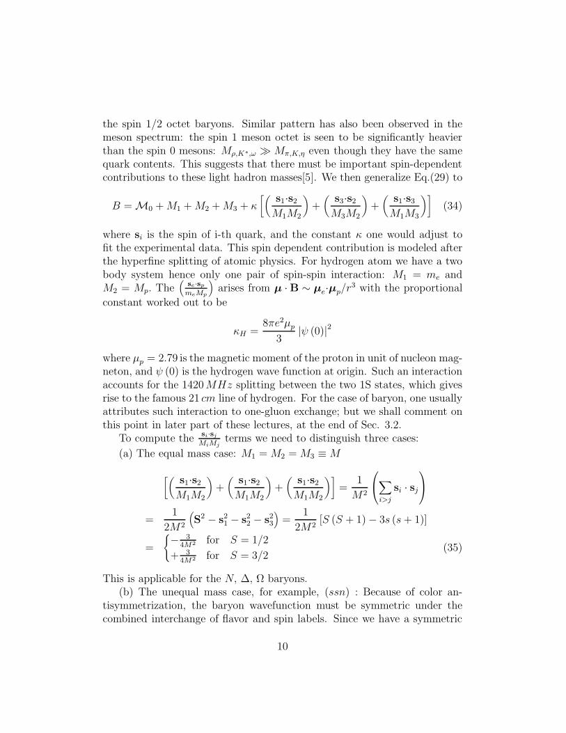
the spin 1/2 octet baryons. Similar pattern has also been observed in themeson spectrum: the spin 1 meson octet is seen to be significantly heavierthan the spin 0 mesons: Mρ,K∗,ω ≫ Mπ,K,η even though they have the samequark contents. This suggests that there must be important spin-dependentcontributions to these light hadron masses[5]. We then generalize Eq.(29) to

B = M0 +M1 +M2 +M3 + κ[(

s1·s2

M1M2

)+(

s3·s2

M3M2

)+(

s1·s3

M1M3

)](34)

where si is the spin of i-th quark, and the constant κ one would adjust tofit the experimental data. This spin dependent contribution is modeled afterthe hyperfine splitting of atomic physics. For hydrogen atom we have a twobody system hence only one pair of spin-spin interaction: M1 = me andM2 = Mp. The

(se·sp

meMp

)arises from µ ·B ∼ µe·µp/r

3 with the proportional

constant worked out to be

κH =8πe2µp

3|ψ (0)|2

where µp = 2.79 is the magnetic moment of the proton in unit of nucleon mag-neton, and ψ (0) is the hydrogen wave function at origin. Such an interactionaccounts for the 1420MHz splitting between the two 1S states, which givesrise to the famous 21 cm line of hydrogen. For the case of baryon, one usuallyattributes such interaction to one-gluon exchange; but we shall comment onthis point in later part of these lectures, at the end of Sec. 3.2.

To compute thesi·sj

MiMjterms we need to distinguish three cases:

(a) The equal mass case: M1 = M2 = M3 ≡M

[(s1·s2

M1M2

)+(

s1·s2

M1M2

)+(

s1·s2

M1M2

)]=

1

M2

∑

i>j

si · sj

=1

2M2

(S2 − s2

1 − s22 − s2

3

)=

1

2M2[S (S + 1) − 3s (s+ 1)]

=

− 3

4M2 for S = 1/2

+ 34M2 for S = 3/2

(35)

This is applicable for the N, ∆, Ω baryons.(b) The unequal mass case, for example, (ssn) : Because of color an-

tisymmetrization, the baryon wavefunction must be symmetric under thecombined interchange of flavor and spin labels. Since we have a symmetric

10

superposition of flavor states, the subsystem (ss) must have spin 1, Namely,ss · ss = 1

2(2 − 2s2

s) = 14, and

2ss · sn =

∑

i>j

si · sj− ss · ss =

−3

4− 1

4= −1 for S = 1/2

+34− 1

4= +1

2for S = 3/2

or[(

s1·s2

M1M2

)+(

s1·s2

M1M2

)+(

s1·s2

M1M2

)]=

[(ss·ssM2

s

)+ 2

(ss·snMsMn

)]

=

14M2

s− 1

MsMnfor S = 1/2

14M2

s+ 1

2MsMnfor S = 3/2

(36)

This case is applicable to Ξ and Ξ∗, as well as Σ and Σ∗ because the sigmabaryons are isospin I = 1 states (hence symmetric in the nonstrange flavorspace).

(c) The Λ baryon: Because Λ is an isoscalar, the subsystem must be inspin 0 state. From this one can easily work out the spin factor to be − 3

4M2n,

independent of Ms.Putting all this together into Eq.(34) we obtain, for the octet baryons:

N = M0 + 3Mn −3κ

4M2n

(37)

Λ = M0 + 2Mn +Ms −3κ

4M2n

Σ = M0 + 2Mn +Ms +κ

4M2n

− κ

MsMn

Ξ = M0 +Mn + 2Ms +κ

4M2s

− κ

MsMn

and for the decuplet baryons:

∆ = M0 + 3Mn +3κ

4M2n

(38)

Σ∗ = M0 + 2Mn +Ms +κ

4M2n

+κ

2MsMn

Ξ∗ = M0 +Mn + 2Ms +κ

4M2s

+κ

2MsMn

Ω = M0 + 3Ms +3κ

4M2s

.

11

One can obtain an excellent fit (within 1%) to all the masses with the pa-rameter values (e.g. [6]) M0 = 0, κ

M2n

= 50MeV and the constituent quarkmass values of

Mn = 363 MeV, Ms = 538MeV. (39)

Similarly good fit can also be obtained for mesons, with an enhancedvalue of κ. Besides some different coupling factors this may reflect a larger|ψ (0)|2 ∝ R−3, which is compatible with the observed root mean squarecharge radii of mesons vs baryons: Rmeson ≃ 0.6 fm vs Rbaryon ≃ 0.8 fm.

1.3.2 Spin and magnetic moments of the baryon

Another useful tool to study hadron structure is the magnetic moment of thebaryon. Their deviation from the Dirac moments values (eB/2MB) indicatesthe presence of structure. In the quark model the simplest possibility is thatthe baryon magnetic moment is simply the sum of its constituent quark’sDirac moments. Clearly, the magnetic moments are intimately connected tothe spin structure of the hadron. Hence, we shall first make a detour into adiscussion of the baryon spin structure in the constituent quark model.

Quark contributions to the proton spin Because it is antisymmetricunder the interchange of quark color indices, the baryon wavefunction mustbe symmetric in the spin-flavor space. Mathematically, we say that thebaryon wavefunction should be invariant under the permutation group S3 —the group of permuting three quarks with spin and isospin labels.

We shall concentrate on the case of proton. While the product wavefunc-tion is symmetric, the individual spin and isospin wavefunctions are of themixed-symmetry type. There are two mixed-symmetry spin-1

2wavefunction

combinations:

(i) χS — symmetric in the first two quarks: Namely, the first twoquarks form a spin 1 subsystem: (Notation for the spin-up and

-down states:∣∣∣12,+1

2

⟩≡ α and

∣∣∣12,−1

2

⟩≡ β)

|1,+1〉 = α1α2, |1, 0〉 =1√2

(α1β2 + β1α2) , |1,−1〉 = β1β2

which is combined with the 3rd quark to form a spin 12

proton:

∣∣∣∣1

2,+

1

2

⟩

S=

√2

3|1,+1〉

∣∣∣∣1

2,−1

2

⟩−√

1

3|1, 0〉

∣∣∣∣1

2,+

1

2

⟩

12

or

χS =1√6(2α1α2β3 − α1β2α3 − β1α2α3). (40)

(ii) χA — antisymmetric in the first two quarks: The first twoquarks form a spin 0 subsystem:

∣∣∣∣1

2,+

1

2

⟩

A= |0, 0〉

∣∣∣∣1

2,+

1

2

⟩

or

χA =1√2(α1β2 − β1α2)α3. (41)

While χS,A are the spin-12

wavefunctions, with identical steps, we canconstruct the two mixed-symmetry isospin-1

2wavefunctions χ′S,A :

χ′S =1√6(2u1u2d3 − u1d2u3 − d1u2u3)

χ′A =1√2(u1d2 − d1u2)u3. (42)

Both the spin wavefunctions (χS χA) and the isospin wavefunctions (χ′S χ′A)

form a two dimensional representation of the permutation group S3. Forexample, under the permutation operations of P12 and P13

P12

(χSχA

)=

(1 00 −1

)

︸ ︷︷ ︸M12

(χSχA

)P13

(χSχA

)=

(−1

2−√

32

−√

32

+12

)

︸ ︷︷ ︸M13

(χSχA

)

where Mij are 2-dimensional representations in terms of orthogonal matrices.Consequently, we find that the combinations such as (χ2

S + χ2A) , (χ′2S + χ′2A)

and (χSχ′S + χAχ

′A) are invariant under S3 transformations. In this way we

find the symmetric proton spin-isospin wavefunction:

|p+〉 =1√2

(χSχ′S + χAχ

′A) (43)

=1√2[1

6(2α1α2β3 − α1β2α3 − β1α2α3)(2u1u2d3 − u1d2u3 − d1u2u3)

+1

2(α1β2α3 − β1α2α3)(u1d2u3 − d1u2u3)]

13

=1

6√

2[4 (u+u+d− + u+d−u+ + d−u+u+)

−2(u+u−d+ + u−d+u+ + d+u+u−

+u−u+d+ + u+d+u− + d+u−u+)]

where we have used the notation of αu = u+, βd = d−, etc. In calculatingphysical quantities, many terms, e.g. u+u+d−, u+d−u+ and d−u+u+ yieldthe same contribution. Hence we can use the simplified wavefunction:

|p+〉 =1√6(2u+u+d− − u+u−d+ − u−u+d+) (44)

From this we can count the number of quark flavors with spin parallel orantiparallel to the proton spin:

u+ =5

3, u− =

1

3, d+ =

1

3, u− =

2

3(45)

summing up to two u and one d quarks. From the difference

∆q = q+ − q− (46)

we also obtain the contribution by each of the quark flavors to the protonspin:

∆u =4

3∆d = −1

3∆s = 0, and ∆Σ = 1, (47)

where ∆Σ = ∆u+ ∆d+ ∆s is the sum of quark polarizations.

Quark contributions to the baryon magnetic moments Instead ofproceeding directly to the results of quark model calculation of the baryonmagnetic moments, we shall first set up a more general framework. This willbe useful when we consider the contribution from the quark sea in the laterpart of these lectures. We shall pay special attention to the contribution byantiquarks. If there are antiquarks in the proton, the definition in Eq.(46)becomes

∆q = (q+ − q−) + (q+ − q−) ≡ ∆q + ∆q (48)

Thus the quark spin contribution ∆q is the sum of the quark and antiquarkpolarizations. For the q-flavor quark contribution to the proton magneticmoment, we have however

µp (q) = ∆qµq + ∆qµq = (∆q − ∆q)µq ≡ ∆qµq (49)

14

where µq is the magnetic moment of the q-flavor quark. The negative signsimply reflects the opposite quark and antiquark moments, µq = −µq. Thusthe spin factor that enters into the expression for the magnetic moment is∆q, the difference of the quark and antiquark polarizations. If we assumethat the proton magnetic moment is entirely built up from the light quarksinside it, we have

µp = ∆uµu + ∆dµd + ∆sµs. (50)

In such an expression there is a separation of the intrinsic quark magneticmoments and the spin wavefunctions. Flavor-SU(3) symmetry then implies,the proton wavefunction being related the Σ+ wavefunction by the inter-change of d ↔ s and d ↔ s quarks, the relations

(∆u

)Σ+

=(∆u

)p≡ ∆u,

(∆d

)Σ+

= ∆s, and(∆s)

Σ+= ∆d; similarly it being related to the Ξ0 wave-

function by a further interchange of u↔ s quarks, thus(∆d

)Ξ0

=(∆d

)Σ+

=

∆s,(∆s)

Ξ0=(∆u

)Σ+

= ∆u, and(∆u

)Ξ0

=(∆s)

Σ+= ∆d. We have,

µΣ+ = ∆uµu + ∆sµd + ∆dµs, (51)

µΞ0 = ∆dµu + ∆sµd + ∆uµs, (52)

the intrinsic moments µq being unchanged when we go from Eq.(50) toEqs.(51) and (52). The n, Σ−, and Ξ− moments can be obtained fromtheir isospin conjugate partners p,Σ+, and Ξ0 by the interchange of theirrespective u↔ d quarks:

(∆u

)Σ−

=(∆d

)Σ+

= ∆s, etc.

µn = ∆dµu + ∆uµd + ∆sµs, (53)

µΣ− = ∆sµu + ∆uµd + ∆dµs, (54)

µΞ− = ∆sµu + ∆dµd + ∆uµs. (55)

The relations for the Iz = 0, Y = 0 moments are more complicated inappearance but the underlying arguments are the same.

µΛ =1

6

(∆u+ 4∆d+ ∆s

)(µu + µd) (56)

+1

6

(4∆u− 2∆d+ 4∆s

)µs,

µΛΣ =−1

2√

3

(∆u− 2∆d+ ∆s

)(µu − µd) . (57)

15

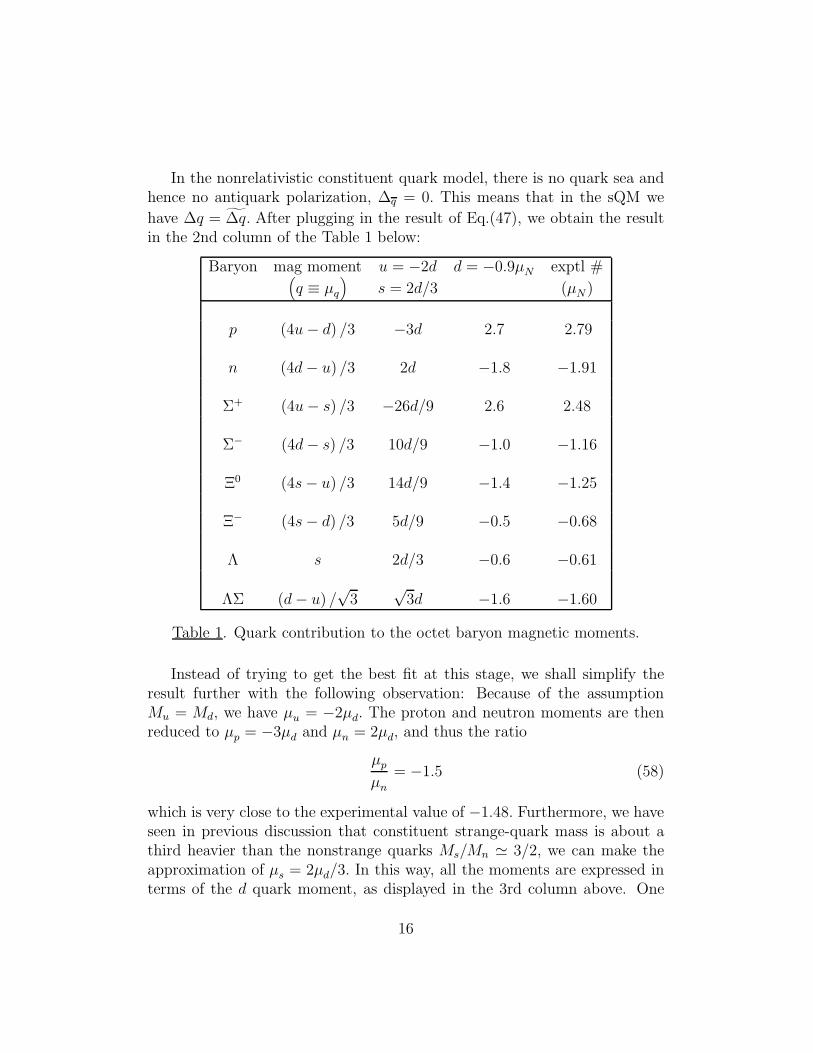
In the nonrelativistic constituent quark model, there is no quark sea andhence no antiquark polarization, ∆q = 0. This means that in the sQM we

have ∆q = ∆q. After plugging in the result of Eq.(47), we obtain the resultin the 2nd column of the Table 1 below:

Baryon mag moment u = −2d d = −0.9µN exptl #(q ≡ µq

)s = 2d/3 (µN )

p (4u− d) /3 −3d 2.7 2.79

n (4d− u) /3 2d −1.8 −1.91

Σ+ (4u− s) /3 −26d/9 2.6 2.48

Σ− (4d− s) /3 10d/9 −1.0 −1.16

Ξ0 (4s− u) /3 14d/9 −1.4 −1.25

Ξ− (4s− d) /3 5d/9 −0.5 −0.68

Λ s 2d/3 −0.6 −0.61

ΛΣ (d− u) /√

3√

3d −1.6 −1.60

Table 1. Quark contribution to the octet baryon magnetic moments.

Instead of trying to get the best fit at this stage, we shall simplify theresult further with the following observation: Because of the assumptionMu = Md, we have µu = −2µd. The proton and neutron moments are thenreduced to µp = −3µd and µn = 2µd, and thus the ratio

µpµn

= −1.5 (58)

which is very close to the experimental value of −1.48. Furthermore, we haveseen in previous discussion that constituent strange-quark mass is about athird heavier than the nonstrange quarks Ms/Mn ≃ 3/2, we can make theapproximation of µs = 2µd/3. In this way, all the moments are expressed interms of the d quark moment, as displayed in the 3rd column above. One

16

can then make a best over-all-fit to the experimental values by adjusting thislast parameter µd. The final results, in column 4, are obtained by takingµd = −0.9µN , where µN is nucleon magneton e/2MN . They are compared,quite favorably, with the experimental values in the last column. We alsonote that, with the d quark having a third of the electronic charge, the fit-parameter of µd = −0.9µN translates into a d quark constituent mass of

Mn =MN

3 × 0.9= 348MeV, and Ms =

3Mn

2= 522MeV, (59)

which are entirely compatible with the constituent quark mass values inEq.(39), obtained in fitting the baryon masses by including the spin-dependentcontributions.

1.3.3 sQM lacks a quark sea

So far we have discussed the successes of the simple quark model. Thereare several instances which indicate that this model is too simple: sQM doesnot yield the correct nucleon matrix elements of the axial vector and scalardensity operators.

Axial vector current matrix elements The quark spin contribution toproton ∆q in Eq.(48) is just the proton matrix element of the quark axialvector current operator

2sµ∆q =⟨p, s

∣∣∣qγµγ5q∣∣∣ p, s

⟩= 2sµ (q+ − q− + q+ − q−) (60)

where sµ is the spin-vector of the nucleon, as the axial current vector corre-sponds to the non-relativistic spin operator:

qγγ5q = q†(

σ 00 σ

)q. (61)

Through SU (3) these matrix elements can be related to the axial vectorcoupling as measured in the octet baryon beta decays. In particular, wehave

(∆u− ∆d)exptl = 1.26

(∆u+ ∆d− 2∆s)expt = 0.6 (62)

17

which is to be compared to the sQM results of Eq.(47):

(∆u− ∆d)sQM = 5/3

(∆u+ ∆d − 2∆s)sQM = 1. (63)

Scalar density matrix elements The matrix elements of scalar densityoperator qq can be interpreted as number counts of a quark flavor in proton

〈p |qq| p〉 = q + q (64)

where q (q) on the RHS denotes the number of a quark (antiquark) flavorin a proton. Namely, the proton matrix element of the scalar operator qqmeasures the sum of quark and antiquark number in the proton (opposed tothe difference q − q as measured by q†q ). It is useful to define the fractionof a quark-flavor in a proton as

F (q) =〈p |qq| p〉⟨

p∣∣∣uu+ dd+ ss

∣∣∣ p⟩ . (65)

We already have calculated proton matrix element of the scalar density inthe subsection on the baryon masses, Eqs.(21) and (20). Thus we have

F (3)

F (8)=

F (u) − F (d)

F (u) + F (d) − 2F (s)=

α

α− 2β(66)

The parameters (α, β) can be deduced from Eq.(22) in the SU (3) symmetriclimit (m3u3 = 0) , as

α =MΣ −MΞ

3m8β =

MΣ −MN

3m8

Thus the ratio[F (3)

F (8)

]

exptl

=MΣ −MΞ

2MN −MΣ −MΞ= 0.23 (67)

which is to be compared to the sQM value of[F (3)

F (8)

]

sQM

=1

3. (68)

The simplest interpretation of these failures is that the sQM lacks a quark sea.Hence the number counts of the quark flavors does not come out correctly.

18

1.4 The OZI rule

The simple quark model of hadron structure discussed above ignores thepresence of quark sea. Even when the issue of the quark sea in nonstrangehadrons is discussed, its (ss) component is usually assumed to be highlysuppressed. This is based on the OZI-rule[7], which was first deduced frommeson mass spectra. In this Subsection we briefly review this topic.

1.4.1 The OZI rule for mesons

The three (qq) combinations that are diagonal in light-quark flavors are thetwo isospin I = 1 and 0 states of a flavor-SU(3) octet together with a SU(3)singlet. Isospin being a good flavor symmetry, there should be very littlemixing between the I = 1 and 0 states. On the other hand, the flavor-SU(3)being not as a good symmetry, we anticipate some mixing between the octet-and the singlet- I = 0 states:

|8〉 =1√6

(uu+ dd− 2ss

)|0〉 =

1√3

(uu+ dd+ ss

)(69)

Pseudoscalar meson masses and mixings The Gell-Mann-Okubo massrelation for the 0− mesons, before the identification of η as the 8th memberof the octet, may be interpreted as giving the mass of this 8th meson:

m28 =

1

3

(4m2

K −m2π

)= (567MeV )2 (70)

which is much closer to the η meson mass of mη = 547MeV than mη′ =958MeV. The small difference m8 −mη can be attributed to a slight mixingbetween the octet and singlet isoscalars. Namely, we interpret η and η′

mesons as two orthogonal combinations of |8〉 and |0〉 with a mixing anglethat can be determined as follows:

(m2

8 m208

m280 m2

0

)=

(cos θ sin θ

− sin θ cos θ

)(m2η 0

0 m2η′

)(cos θ − sin θsin θ cos θ

).

Hence

sin2 θP =m2

8 −m2η

m2η′ −m2

η

i.e. a small θP ≃ 11o. (71)

19

Vector meson masses and mixings We now apply the same calculationto the case of vector mesons:

m∗28 =1

3

(4m2

K∗ −m2ρ

)= (929MeV )2

which is to be compared to the observed isoscalar vector mesons of ω (782MeV )and φ (1020MeV ) . This implies a much more substantial mixing. The diag-onalization of the corresponding mass matrix:

(m∗28 m∗208m∗280 m∗20

)−→

(m2ω 0

0 m2φ

)

requires a mixing angle of

sin2 θV =m∗28 −m2

ω

m2φ −m2

ω

or θV ≃ 50o. (72)

The physical states should then be

|ω〉 = cos θV |8〉 + sin θV |0〉 |φ〉 = − sin θV |8〉 + cos θV |0〉 . (73)

After substituting in Eqs.(69) and (72) into Eq.(73), we have

|ω〉 = 0.7045∣∣∣uu+ dd

⟩+0.0857 |ss〉 |φ〉 = −0.06

∣∣∣uu+ dd⟩+0.996 |ss〉 .

This shows that ω has little s quarks, while the φ mesons is vector mesoncomposed almost purely of s quarks. Such a combination is close to thesituation of “ideal mixing”, corresponding to an angle of θ0 ≃ 55o, with thenon-strange and strange quarks being completely separated:

|ω〉 =1√2

∣∣∣uu+ dd⟩

|φ〉 = |ss〉 . (74)

The OZI rule It is observed experimentally that the φ meson decay pre-dominantly into strange-quark-bearing final states, even though the phasespace, with mφ > mω, favors its decay into nonstrange pions final states:

ω → 3π 89% φ → KK 83%→ ρπ 13%→ 3π 3%

20

with a ratio of partial decay widths Γ(φ→ 3π)/Γ(ω → 3π) = 0.014.This property of the hadron decays has been suggested to imply a strong

interaction regularity: the OZI-rule — the annihilations of the ss pair viastrong interaction are suppressed[7]. We remark that this suppression shouldbe interpreted as a suppression of the coupling strength rather than a phasespace suppression due to the larger strange quark mass (i.e. it is above andbeyond the conventional flavor SU(3) breaking effect.)

The extension of the OZI-rule to heavy quarks of charm and bottom hasbeen highly successful. For example it explains the extreme narrowness of theobserved J/ψ width because this (cc) bound state is forbidden to decay intothe OZI-allowed channel of DD because, with a mass of mJ/ψ ≃ 3100MeV,it lies below the threshold of 2mD ≃ 3700MeV.

From the viewpoint of QCD, applications of the OZI-rule to the heavyc, b, and t quarks are much less controversial than those for strange quarks —even thought the rule was originally “discovered” in the processes involvings quarks. For heavy quarks, this can be understood in terms of perturbativeQCD and asymptotic freedom[8]. It is not the case for the s quark which,as evidenced by the success of flavor-SU(3) symmetry, should be considereda light quark. Furthermore, the phenomenological applications of the OZIto strange quark processes have not been uniformly successful. In contrastto the case of vector mesons Eq.(72), there is no corresponding success forthe pseudoscalar mesons — as evidenced by the strong deviation from idealmixing in the η and η′ meson system, Eq.(71).

1.4.2 The OZI rule and the strange quark content of the nucleon

A straightforward application of the s quark OZI rule to the baryon is thestatement that operators that are bilinear in strange quark fields shouldhave a strongly suppressed matrix elements when taken between nonstrangehadron states such as the nucleon. In particular we expect the fraction of squarks in a nucleon, Eq.(65), should be vanishingly small.

F (s) =s+ s

∑(q + q)

=〈N |ss|N〉⟨

N∣∣∣uu+ dd+ ss

∣∣∣N⟩ ≃ 0. (75)

The “measured” value of the pion-nucleon sigma term[9]:

σπN = mn

⟨N∣∣∣uu+ dd

∣∣∣N⟩

(76)

21

and the SU(3) relation

M8 ≡ m8 〈N |u8|N〉 =1

3(mn −ms)

⟨N∣∣∣uu+ dd− 2ss

∣∣∣N⟩

= MΛ −MΞ ≃ −200MeV, (77)

which is obtained from Eqs.(20) and (22) in the isospin invariant limit (m3u3 = 0) ,allow us to make a phenomenological estimate of the strange quark contentof the nucleon[10]: We can rewrite the expression in Eq.(75) as

F (s) =

⟨N∣∣∣(uu+ dd

)−(uu+ dd− 2ss

)∣∣∣N⟩

⟨N∣∣∣3(uu+ dd

)−(uu+ dd− 2ss

)∣∣∣N⟩

=σπN − 25MeV

3σπN − 25MeV(78)

where we have used (77) and the current quark mass ratiom8/ms = −8 corre-sponding toms/mn = 25 of Eq.(9). Thus the validity of OZI rule, F (s) = 0,would predict, through (78), that σπN should have a value close to 25MeV.However, the commonly accepted phenomenological value[11] is more like45MeV, which translates into a significant strange quark content in the nu-cleon:

F (s) ≃ 0.18. (79)

We should however keep in mind that this number is deduced by using flavorSU (3) symmetry. Hence the kinematical suppression effect of Ms > Mn hasnot been taken into account.

2 Deep Inelastic Scatterings

2.1 Polarized lepton-nucleon scatterings

There is a large body of work on the topic of probing the proton spin structurethrough polarized deep inelastic scattering (DIS) of leptons on nucleon target.The reader can learn more details by starting from two excellent reviews of[12] and [13].

22

2.1.1 Kinematics and Bjorken scaling

For a lepton (electron or muon) scattering off a nucleon target to producesome hadronic final state X, via the exchange of a photon (4-momentumqµ), the inclusive cross section can be written as a product

dσ (l +N → l +X) ∝ lµνWµν (80)

where lµν is the known leptonic part while Wµν is the hadronic scatteringamplitude squared,

∑X |T (γ∗ (q) +N (p) → X)|2 , which is given, accord-

ing to the optical theorem, by the imaginary part of the forward Comptonamplitude:

Wµν =1

2πIm

∫ ⟨p, s

∣∣∣T(Jemµ (x) Jemν (0)

)∣∣∣ p, s⟩eiq·xd4x

=

(−gµν +

qµqνq2

)F1

(q2, ν

)+

(pµ −

p · qq2

qµ

)(pν −

p · qq2

qν

)F2 (q2, ν)

p · q

+iǫµναβqα

[sβg1 (q2, ν)

p · q + p · q sβ − s · q pβ g2 (q2, ν)

(p · q)2

](81)

whereq2 ≡ −Q2 < 0 and ν =

p · qM

(82)

M being the nucleon mass. sα = uN (p, s) γαγ5uN (p, s) is the spin-vector ofthe proton, and the variable ν is the energy loss of the lepton, ν = E − E ′.We have defined the spin-independent F1,2 (q2, ν) and the spin-dependentg1,2 (q2, ν) structure functions. In particular, the cross section asymmetrywith the target nucleon spin being anti-parallel and parallel to the beam oflongitudinally polarized leptons is given by the structure function g1 :

dσ↑↓

dxdy− dσ↑↑

dxdy=e4ME

πQ4xy (2 − y) g1 +O

(M2

Q2

)(83)

where x = Q2

2νMand y = ν

E. In practice one measures g1 via the (longitudinal)

spin-asymmetry,

A1 =dσ↑↑ − dσ↑↓

dσ↑↑ + dσ↑↓≃ 2x

g1

F2

. (84)

in the kinematic regime of ν ≫√Q2.

To probe the nucleon structure at small distance scale we need to goto the large energy and momentum-transfer deep inelastic region — large

23

Q2 and ν, with fixed x. In the configuration space, this corresponds to thelightcone regime. The statement of Bjorken scaling is that, in this kinematiclimit, the structure functions approach non-trivial functions of one variable:

F1,2

(q2, ν

)→ F1,2 (x) , g1,2

(q2, ν

)→ g1,2 (x) . (85)

Such problems can be studied with the formal approach of operator productexpansion, which has a firm field theoretical-foundation in QCD, or the moreintuitive approach of parton model, which can lead to considerable insightabout the hadronic structure.

2.1.2 Inclusive sum rules via operator product expansion

The forward Compton amplitude Tµν is the matrix element, taken betweenthe nucleon states

Tµν = 〈p, s |tµν | p, s〉 , (86)

of the time-order product of two electromagnetic current operators

tµν = i∫d4x eiq·xT (Jµ (x) Jν (0)) . (87)

It is useful to express the product of two operators at short distances asan infinite series of local operators, OA (x)OB (0) =

∑i Ci (x)Oi (0), as it

is considerably simpler to work with the matrix elements of local operatorsOi (0). For DIS study we are interested in the lightcone limit x2 → 0. Henceoperators of all possible dimensions (di) and spins (n) are to be included:

OA (x)OB (0) =∑

i,n

Ci(x2)xµ1

...xµnOµ1...µni (0) (88)

where Oµ1...µn

i (0) is understood to be a symmetric traceless tensor operator(corresponding to a spin n object). From dimension analysis we see that thecoefficient

Ci(x2)∼(√

x2)τ i−dA−dB

where τ i = di − n is the twist of the local operator Oµ1...µni (0) . Thus in the

lightcone limit x2 → 0, the most important contributions come from thoseoperators with the lowest twist values.

In the short distance scale, the QCD running coupling is small so that per-turbation theory is applicable. In this way the c-numbers coefficients Ci (x

2)

24

can be calculated with the local operators Oµ1...µni (0) being the composite

operators of the quark and gluon fields.We are interested, as in Eq.(87), in the operator products in the momen-

tum space. Namely, the above discussion has to be Fourier transformed fromconfiguration space into the momentum space: x → q, with the relevant limitbeing Q2 → ∞. The spin-dependent case corresponds to an operator productantisymmetric in the Lorentz indices µ and ν :

t[µν] =∑

ψ,n=1,3,...

C(3)

(q2, αs

)( 2

−q2

)niǫµναβq

αqµ2....qµn

Oβµ2....µn

A,ψ (89)

where C(3) (q2, αs) = 1+O (αs) , [the subscript (3) reminds us of others terms,

1 & 2, that contribute to the spin-independent amplitudes F1,2]. Oβµ2....µn

A,ψ isa twist-two pseudotensor operator:

Oβµ2....µn

A,ψ = e2ψ

(i

2

)n−1

ψγβ←→D

µ2

....←→D

µn

γ5ψ (90)

where ψ is the quark field with charge eψ. The crossing symmetry property

tµν (p, q) = tνµ (p,−q) (91)

implies that only odd-n terms appear in the [µν] series. (By the same to-ken, only even-n terms contribute to the spin-independent structure functionF1,2.)

The spin-dependent part of the forward Compton amplitude Eq.(86) is

T[µν] =⟨p, s

∣∣∣t[µν]∣∣∣ p, s

⟩= iǫµναβq

αsβg1 (q2, ν)

p · q + ... (92)

Namely, Im g1 (q2, ν) = 2πg1 (q2, ν) . When we sandwich the OPE termsEqs.(89) and (90) into the nucleon states we need to evaluate matrix ele-ment ⟨

p, s∣∣∣Oβµ2....µn

A,ψ

∣∣∣ p, s⟩

= 2e2ψAn,ψsβpµ2 ....pµn (93)

Plug Eqs.(93) and (89) into Eq.(92) we have

iǫµναβqαsβ

g1

p · q =∞∑

n=1,3,...

C(3)

(2

−q2

)niǫµναβq

αsβ (p · q)n−1 2e2ψAn,ψ

25

org1 =

∑

ψ,n

2C(3)e2ψAn,ψω

n (94)

where ω = 2p·q−q2 is the inverse of the Bjorken-x variable. Asymptotic freedom

of QCD has allowed us to express the structure function as a power seriesin ω,Eq.(94) with calculable c number coefficients C(3) and “unknown” longdistance quantities An,ψ. To turn this into a useful relation we need to invertthe summation over n (i.e. to isolate the coefficient An,ψ). For this we canuse the Cauchy’s theorem for contour integration:

1

2πi

∮dωg1 (ω)

ωn+1=∑

ψ

2C(3)e2ψAn,ψ, (95)

which can be related to physical processes by evaluating the LHS integralwith a deformed contour so that it wraps around the two physical cuts,ω = (1,∞) and (−∞,−1) . (The second region corresponding to the cross-channel process.) Using

g1 (ω + iε) − g∗1 (ω + iε) = 2i Im g1 (ω) = 4iπg1 (ω) (96)

and the crossing symmetry property

g1 (p, q) = −g1 (p,−q) or g1

(ω, q2

)= −g1

(−ω, q2

), (97)

we then obtain

1

2πi

∮dωg1 (ω)

ωn+1=

1

π

∫ ∞

1dω

Im g1 (ω)

ωn+1+

1

π

∫ −1

−∞dω

Im g1 (ω)

ωn+1

= 2 [1 − (−1)n]∫ ∞

1dωg1 (ω)

ωn+1= 4

∫ 1

0xn−1g1 (x) dx. (98)

We recall that the spin-index n must be odd. The first-moment (n = 1) sum

∫ 1

0dxg1

(x,Q2

)=

1

2

∑

ψ

C(3)e2ψA1,ψ (99)

is of particular interest because the corresponding matrix element on theRHS can be measured independently, Cf. Eqs.(60) and (93):

2A1sβ =

⟨p, s

∣∣∣ψγβγ5ψ∣∣∣ p, s

⟩≡ 2sβ∆ψ. (100)

26

Without including the higher order QCD corrections in the coefficient, wehave the g1 sum rule for the electron proton scattering:

∫ 1

0dxgp1

(x,Q2

)=

1

2

(4

9∆u+

1

9∆d+

1

9∆s). (101)

For the difference between scatterings on the proton and the neutron targets,we can use the isospin relations (∆u)n = ∆d and (∆d)n = ∆u to get:

∫ 1

0dx[gp1(x,Q2

)− gn1

(x,Q2

)]=

1

6(∆u− ∆d) . (102)

The matrix element on the RHS:

2sβ (∆u− ∆d) =⟨p, s

∣∣∣uγβγ5u− dγβγ5d∣∣∣ p, s

⟩

=⟨p, s

∣∣∣uγβγ5d∣∣∣n, s

⟩= 2sβgA (103)

is simply the axial vector decay constant of neutron beta decay. Includingthe higher order QCD correction to the OPE Wilson coefficient, one can thenwrite down the Bjorken sum rule:

∫ 1

0dx[gp1(x,Q2

)− gn1

(x,Q2

)]=gA6C(NS) (104)

with the non-singlet coefficient[14],

C(NS) = 1 − αsπ

− 43

12

(αsπ

)2

− 20.22(αsπ

)3

+ ... (105)

All experimental data are consistent with this theoretical prediction.

Remark Anomalous dimension and the Q2-dependence: TheQ2-dependenceof the moment integral, such as LHS of Eq.(99), are given by αs (Q2) ∼1/ lnQ2 in the coefficient function and by the Q2-evolution of the oper-ator according to the renormalization group equation[15], which yields

⟨p, s

∣∣∣O|Q∣∣∣ p, s

⟩

⟨p, s

∣∣∣O|Q0

∣∣∣ p, s⟩ =

[αs (Q)

αs (Q0)

] γ2b

(106)

where γ is the anomalous dimension of the operator O and b is theleading coefficient in the QCD β function. The label Q in the matrix

27

elements refers to the mass scale at which the operator is renormalized,chosen at µ2 ≃ Q2 in order to avoid large logarithms. For the g1 sumrule Eq.(99) the Q2-dependence is particularly simple. The non-singletaxial current is (partially) conserved, hence has anomalous dimensionγ = 0. The singlet current is not conserved because of axial anomaly(see discussion below). But it has very weak Q2-dependence becausethe corresponding anomalous dimension starts at the two-loop level.

2.1.3 The parton model approach

The g1 sum rule of Eq.(101) has been derived directly through OPE fromQCD. We can also get this result by using the parton model, which picturesthe target hadron, in the infinite momentum frame, as superposition of quarkand gluon partons each carrying a fraction (x) of the hadron momentum. Forthe short distance processes one can calculate the reaction cross section as anincoherent sum over the rates for the elementary processes. Thus in Comptonscattering, a photon (momentum qµ) strikes a parton (xpµ) turning it into afinal state parton (qµ + xpµ), the initial and final partons must be on shell:

(xpµ)2 = (qµ + xpµ)

2 or x =−q2

2p · q . (107)

Hence the Bjorken-x variable has the interpretation as the fraction of the lon-gitudinal momentum carried by the parton. A simple calculation[16] showsthe scaling structure functions being directly related to the density of partonswith momentum fraction x :

F p2 (x) = x

∑

q=u,d,s

e2q [q (x) + q (x)] (108)

and

gp1 (x) =1

2

∑

q=u,d,s

e2q [q+ (x) − q− (x) + q+ (x) − q− (x)]

=1

2

∑e2q [∆q (x) + ∆q (x)] =

1

2

∑e2q∆q (x) (109)

Thus the spin asymmetry of Eq.(84) has the interpretation as

A1 (x) ≃∑q e

2q [∆q (x) + ∆q (x)]

∑q e2q [q (x) + q (x)]

. (110)

28

Comparing this interpretation of the spin-dependent structure functionto that for the proton matrix elements of the axial vector current Eq.(60),we see that the g1 sum rule Eq.(101) implies the consistency condition of

∫ 1

0q± (x) dx = q±

∫ 1

0q± (x) dx = q±. (111)

In other words, the proton matrix element of the local axial vector current〈p, s |OA,q| p, s〉 can be evaluated, in the partonic language, by taking the axialvector current between quark states (〈q, h |OA,q| q, h〉 = 2h) and multiplyingit by the probability of finding the quark in the target proton:

〈p, s |OA,q| p, s〉 =∑

q,h

〈q, h |OA,q| q, h〉 qh(x) = (∆q)p (112)

where (∆q)p ≡ ∆q

∆q (x) = q+ (x) − q− (x) + q+ (x) − q− (x) ≡ ∆q (x) + ∆q (x) . (113)

Ellis-Jaffe sum rule and the phenomenological values of ∆q Besides

∆u− ∆d = gA = F +D = 1.2573 ± 0.0028, (114)

if we assume flavor SU(3) symmetry, we can fix another octet combination

∆u+ ∆d− 2∆s = ∆8 = 3F −D = 0.601 ± 0.038 (115)

which can be gotten by fitting the axial vector couplings of the hyperon betadecays[17]. In this way Eq.(101) can be written as

Γp =∫ 1

0dxgp1 (x) =

C(NS)

36(3gA + ∆8) +

C(S)

9∆Σ (116)

where ∆Σ = ∆u + ∆d + ∆s. The non-singlet coefficient has been displayedin Eq.(105) while the singlet term has been calculated to be[18]

C(S) = 1 − αsπ

− 1.0959(αsπ

)2

+ ... (117)

If one assume ∆s = 0, thus ∆Σ = ∆8 we then obtain the Ellis-Jaffe sumrule[19] with the RHS of Eq.(116) expected (for αs ≃ 0.25) to be around0.175, had become the baseline of expectation for the spin-dependent DIS.

29

The announcement by EMC collaboration in the late 1980’s that it hadextended the old SLAC result[20] to new kinematic region and obtained anexperimental value for Γp deviated significantly from the Ellis-Jaffe value[21]had stimulated a great deal of activity in this area of research. In particularanother generation of polarized DIS on proton and neutron targets have beenperformed by SMC at CERN[22] and by E142-3 at SLAC[23]. The new datasupported the original EMC findings of ∆s 6= 0 and a much-less-than-unityof the total spin contribution ∆Σ ≪ 1, although the magnitude was not assmall as first thought. The present experimental result may be summarizedas[24]

∆u = 0.82 ± 0.06, ∆d = −0.44 ± 0.06, (118)

∆s = −0.11 ± 0.06, ∆Σ = 0.27 ± 0.11.

The deviation from the simple quark model prediction Eq.(47)

(∆q)exptl < (∆q)sQM (119)

indicates a quark sea strongly polarized in the opposite direction from theproton spin. That the total quark contribution is small means that the protonspin is built up from other components such as orbital motion of the quarksand, if in the relevant region, gluons.

2.1.4 Axial vector current and the axial anomaly

The most widely discussed interpretation of the proton spin problem is thesuggestion that the gluon may provide significant contribution via the axialanomaly[25]. Let us first review some elementary aspects of anomaly. TheSU (3)color gauge symmetry of QCD is of course anomaly-free. The anomalyunder discussion is the one associated with the global axial U (1) symme-try. Namely, the SU (3)-singlet axial current A(0)

µ =∑q=u,d,s qγµγ5q has an

anomalous divergence

∂µA(0)µ =

∑

q=u,d,s

2mq (qiγ5q) + nfαs2πtrGµνGµν (120)

where Gµν is the gluon field tensor, Gµν its dual. nf = 3 is the number ofexcited flavors. For our purpose it is more convenient to express this in termsof each flavor separately.

∂µ(qγµγ5q

)= 2mq (qiγ5q) +

αs2πtrGµνGµν (121)

30

Axial anomaly enters into the discussion of partonic contributions to theproton spin as follows: Because anomaly, being related to the UV regular-ization of the triangle diagram, is a short-distance phenomena, it makes ahard, thus perturbatively calculable (though not the amount), contributionfrom the gluon so that Eq.(112) is modified:

〈p, s |OA,q| p, s〉 =∑

q,h

〈q, h |OA,q| q, h〉Qh(x) +∑

G,h

〈G, h |OA,q|G, h〉Gh (x)

(122)where Gh, just as the quark density Qh being given by Eq.(113), is the spin-dependent gluonic density. The gluonic matrix element of the axial vectorcurrent 〈G, h |OA,q|G, h〉 is just the anomaly triangle diagram which, with〈q, h |OA,q| q, h〉 normalized to ±1, yields a coefficient of ∓αs

2π. In this way the

proton matrix element of the axial vector current is interpreted as being asum of “true” quark spin contribution ∆Q and the gluon spin contribution:

∆q (x) = ∆Q (x) − αs2π

∆G (x) , (123)

where ∆G (x) = G+ (x)−G− (x) . Superficially, the second term is of higherorder. But because the lnQ2 growth of ∆G (due to gluon blemsstrahlungby quarks) compensates for the running coupling αs ∼ (lnQ2)

−1, the com-

bination αs∆G is independent of Q2 at the leading order, and the gluoniccontribution to the proton spin may not be negligible. However in order toobtain the simple quark model result of ∆S = 0, a very large ∆G is required:

− αs2π

∆G = ∆s ≃ −0.1 ⇒ ∆G ≃ 2.5. (124)

2.1.5 Semi-inclusive polarized DIS

From the inclusive lepton nucleon scattering we are able to extract the quarkcontribution to the proton spin, ∆q = ∆q +∆q. Namely, we can only get thesum of the quark and antiquark contributions together. More detailed infor-mation of the spin structure can be obtained from polarized semi-inclusiveDIS, where in addition to the scattered lepton some specific hadron h is alsodetected.

l +N → l + h +X

31

The (longitudinal) spin asymmetry of the inclusive process can be expressedin terms of quark distributions as in Eq.(110):

A1 ≃∑q e

2q (∆q + ∆q)∑q e

2q (q + q)

(125)

Similarly one can measure the spin-asymmetry measured in semi-inclusivecase:

Ah1 ≃

∑q e

2q

(∆qD

hq + ∆qD

hq

)

∑q e

2q

(qDh

q + qDhq

) (126)

where Dhq , the fragmentation function for a quark q to produce the hadron

h, is assumed to be spin-independent. Separating ∆q from ∆q is possible

because Dhq 6= Dh

q . For example, given the quark contents such as π+ ∼(ud)

and π− ∼ (ud), we expect

Dπ+

u ≫ Dπ+

u , Dπ+

d ≫ Dπ+

d , and Dπ−

u ≪ Dπ−

u , Dπ−

d ≪ Dπ−

d

In this way the SMC collaboration[26] made a fit of their semi-inclusive data,in the approximation of ∆u = ∆d and ∆s = ∆s ∝ s (x) (the strange quarkdistribution did not play an important role, and the final result is insensitiveto variation of ∆s). SMC was able to conclude that the polarization of thenon-strange antiquarks is compatible with zero over the full range of x :

∆u = ∆d = −0.02 ± 0.09 ± 0.03 (127)

This is to be compared to their result for ∆q = ∆q − ∆q :

∆u = 1.01 ± 0.19 ± 0.14 ∆d = −0.57 ± 0.22 ± 0.11.

Namely, while the data from inclusive processes suggest that the quark seais strongly polarized — as indicated by the large deviation of measured ∆qfrom their simple quark model prediction Eqs.(118) and (47), the SMC studyof the semi-inclusive processes hints that the antiquarks in the sea are notstrongly polarized.

2.1.6 Baryon magnetic moments

One of the puzzling aspects of the proton spin problem is that, given thesignificant deviation of the quark spin factors ∆q in Eq.(118) from the sQM

32

values, it is hard to see how could the same (∆q)sQM values manage to yieldsuch a good description of the baryon magnetic moments, as shown in Table1.

For this we can only give a partially satisfactory answer : If we assumethat the anitquarks in the proton sea is not polarized ∆q = 0, for whichthe SMC result Eq.(127) gives some evidence (and it is also a predictionof the chiral quark model to be discussed in Sec. 3), we can directly usethe ∆q of Eq.(118) to evaluate the polarization difference: ∆q = ∆q = ∆qin Eq.(49). We can then attempt a fit of the baryon magnetic moments in

exactly the same way we had fit them by using(∆q)sQM

as in Table 1. The

resultant fit, surprisingly, is equally good — in fact better, in the sense oflower χ2[27][28]. Namely, both the sQM ∆q and experimental values of ∆qcan, rather miraculously, fit the same magnetic moment data. In this sense,the new spin structure poses no intrinsic contradiction with respect to themagnetic moment phenomenology.

That it is possible to fit the same baryon magnetic moments with(∆q)sQM

and(∆q)

exptlis due to the fact that the baryon moment, such as Eq.(50), is

a sum of products µB =∑

∆q µq hence different(∆q)′

s can yield the same

µB if(µq)′

s are changed correspondingly. In both cases we have µu = −2µdand µs ≃ −2

3µd. For the sQM case, we find µd ≃ −0.9µN while for the ex-

perimental ∆q case, we need µd ≃ −1.4µN . This shift means a 35% changein the constituent quark mass value — thus a 35% difference with the con-stituent quark mass value obtained from the baryon mass fit in Eq.(39).Consequently, we regard the magnetic moment problem still as an unsolvedpuzzle.

2.2 DIS on proton vs neutron targets

2.2.1 Lepton-nucleon scatterings

The spin-averaged nucleon structure function F2 can be expressed in termsof the quark densities as in Eq.(108)

F p2 (x) = x

[4

9(u+ u) +

1

9

(d+ d

)+

1

9(s+ s)

]

F n2 (x) = x

[4

9

(d+ d

)+

1

9(u+ u) +

1

9(s+ s)

],

33

where we have used the isospin relations of (u)p = (d)n and (d)p = (u)n .Their difference is

1

x[F p

2 (x) − F n2 (x)] =

1

3

[(u− d) +

(u− d

)]

=1

3

[2I3 + 2

(u− d

)]

where I3 = 12

[(u− d) −

(u− d

)]with it integral being the third component

of the isospin:∫ 10 dxI3 (x) = 1

2. The simple assumption that u = d in the

quark sea, which is consistent with it being created by the flavor-independentgluon emission, then leads the Gottfried sum rule[29]

IG =∫ 1

0

dx

x[F p

2 (x) − F n2 (x)] =

1

3. (128)

Experimentally, NMC found that, with a reasonable extrapolation in thevery small-x region, the integral IG deviated significantly from one-third[30]:

IG = 0.235 ± 0.026 =1

3+

2

3

∫ 1

0

[u (x) − d (x)

]dx. (129)

This translates into the statement that, in the proton quark sea, there aremore d-quark pairs as compared to the u-quark pairs.

u− d = −0.147 ± 0.026. (130)

Remark Gottfried sum rule does not follow directly from QCD without ad-ditional assumption. Unlike the g1 sum rule, the Gottfried sum rule cannot be derived from QCD via operator product expansion. A simple wayto see this: Because the spin-independent structure function F2 has op-posite crossing symmetry property from that of g1, only even-n termscan contribute. Hence there is no way to obtain a non-trivial relationfor the odd-n moment sums of F2 (which the Gottfried sum rule wouldbe an example). But in the context of parton model, the Gottfried sumprovides us with an important measure of the flavor structure of theproton quark sea.

2.2.2 Drell-Yan processes

Because to conclude that NMC data showing a violation of the Gottfriedsum rule one needs to make an extrapolation into the small-x regime, an

34

independent confirmation of u 6= d would be helpful. A measurement of thedifference of the Drell-Yan process of proton pN → l+l−X on proton andneutron targets can detect the antiquark density because in such a processthe massive (l+l−) pair is produced by (qq) annihilations[31].

Let us denote the differential cross sections as

σpN ≡ d2σ (pN → l+l−X)

d√τdy

=8πα

9√τ

∑

q=u,d,s

e2q[qP (x1) q

T (x2) + qP (x1) qT (x2)

](131)

where√τ = M√

swith

√s being the CM collision energy andM is the invariant

mass of the lepton pair. y being the rapidity, the fraction of momentumcarried by the parton in the projectile (P ) is given by x1 =

√τey and the

fraction in the target (T ) given by x2 =√τe−y. Explicitly writing out the

quark densities of Eq.(131):

σpp =8πα

9√τ

4

9[u (x1) u (x2) + u (x1) u (x2)] +

1

9

[d (x1) d (x2) + d (x1) d (x2)

]+ s term

σpn =8πα

9√τ

4

9

[u (x1) d (x2) + u (x1) d (x2)

]+

1

9

[d (x1) u (x2) + d (x1)u (x2)

]+ s term

In this way the DY cross section asymmetry can be found:

ADY =σpp − σpn

σpp + σpn

=[4u (x1) − d (x1)]

[u (x2) − d (x2)

]+ [u (x2) − d (x2)]

[4u (x1) − d (x1)

]

[4u (x1) + d (x1)][u (x2) + d (x2)

]+ [u (x2) + d (x2)]

[4u (x1) + d (x1)

]

=(4λ− 1)

(λ− 1

)+ (λ− 1)

(4λ− 1

)

(4λ+ 1)(λ+ 1

)+ (λ+ 1)

(4λ+ 1

) (132)

where λ (x) = u (x) /d (x) and λ (x) = u (x) /d (x) . Thus with measurementsofADY and data fit for λ in the range of (2.0, 2.7) , the NA51 Collaboration[32]obtained, at kinematic point of y = 0 and x1 = x2 = x = 0.18, the ratio ofantiquark distributions to be

u/d = 0.51 ± 0.04 ± 0.05 (133)

confirming that there are more (by a factor of 2) d -quark pairs than u-quarkpairs.

35

3 The Proton Spin-Flavor Structure in the

Chiral Quark Model

3.1 The naive quark sea

A significant part of the nucleon structure study involves non-perturbativeQCD. As the structure problem may be very complicated when viewed di-rectly in terms of the fundamental degrees of freedom (current quarks andgluons), it may well be useful to separate the problem into two stages. Onefirst identifies the relevant degrees of freedom (DOF) in terms of which thedescription for such non-perturbative physics will be simple, intuitive andphenomenologically correct; at the next stage, one then elucidates the rela-tions between these non-perturbative DOFs in terms of the QCD quarks andgluons. Long before the advent of the modern gauge theory of strong inter-action, we have already gained insight into the nucleon structure with thesimple nonrelativistic constituent quark model (sQM). This model pictures anucleon as being a compound of three almost free u- and d -constituent quarks(with masses, much larger than those of current quarks, around a third of thenucleon mass) enclosed within some simple confining potential. There aremany supporting evidence for this picture. We have reviewed some of this inSec. 1. Also, the nucleon structure functions in the large momentum fractionx region, where the valence quarks are expected to be the dominant physicalentities, are invariably found to be compatible with them being evolved froma low Q2 regime described by sQM. For this aspect of the quark model werefer the reader to Ref.[33].

However in a number of instances where small x region can contributeone finds the observed phenomena to be significantly different from thesesQM expectations. This has led many people to call sQM the ”naive quarkmodel” and to suggest a rethinking of the nucleon structure. But we wouldargue that the approach is correct, and only the generally expected featuresof the quark-sea are too simple. This ”naive quark-sea” (nQS) is supposedto be composed exclusively of the u and d quark pairs. Namely, based on thenotion of OZI rule, one would anticipate a negligibly small presence of thestrange quark pairs inside the nucleon. This implies, as given in Eq.(78), apion-nucleon sigma term value of σπN ≃ 25MeV. Furthermore, the similarityof the u and d quark masses and the flavor-independent nature of the gluoncouplings led some people to expect that d = u, thus to the validity of the

36

Gottfried sum rule, Eq.(128).In the sQM, there is no quark-sea and the proton spin is build up entirely

by the valence quark spins. We have deduced the quark contributions to theproton spin as in Eq.(47), which leads to an axial-vector coupling strengthof gA = ∆u − ∆d = 5/3. If one introduces a quark-sea, the nQS feature ofs ≃ 0 (thus ∆s ≃ 0) leads us to the Ellis-Jaffe sum rule,

∫ 10 dxg

p1 (x) = 0.175.

Phenomenologically none of these nQS features

Features of the naive quark seaflavor : s = 0 and d = uspin : ∆s = 0 (∆q = ∆q)sea

have been found to be in agreement with experimental observations. As farback as 1976, the connection of the σπN value to the strange quark contentof the nucleon has been noted. It was pointed out that the then generallyaccepted phenomenological value of 60MeV differed widely from the OZIexpectation[10]. In recent years, the σπN value has finally settled down toa more moderate value of σπN ≃ 45MeV when a more reliable calculationconfirmed the existence of a significant correction due to the two-pion cut[11].Nevertheless, this reduced value still translates into a nucleon strange quarkfraction of 0.18, see Eq.(79).

As for the proton spin, starting with EMC in the 1980’s, the polarizedDIS experiments of leptons on proton target have shown that Ellis-Jaffe sumrule is violated. The first moment the spin-dependent structure function g1

has allowed us to obtain the individual ∆q of Eq.(118). We have alreadynoted that they are all less than the sQM values of Eq.(47), suggesting thatfor each flavor the quark-sea is polarized strongly in the opposite directionto the proton spin.

∆q = (∆q)sQM + (∆q)sea < (∆q)sQM⇒ (∆q)sea < 0.

Furthermore, the recent SMC data on the semi-inclusive DIS scattering[26]tentatively suggested ∆u ≃ ∆d ≃ 0. Thus while the inclusive experimentspoint to a negatively polarized quark sea, the semi-inclusive result indicatesthat the antiquarks in this sea are not polarized.

The NMC measurement of the muon scatterings off proton and neutrontargets shows that the Gottfried sum rule is violated[30]. It has been inter-preted as showing d > u in the proton. This conclusion has been confirmed

37

by the asymmetry measurement (by NA51[32]) in the Drell-Yan processeswith proton and neutron targets, which yield, at a specific quark momentumfraction value (x = 0.18), the result of d ≃ 2u in Eq.(133).

To summarize, the quark-sea is ”observed” to be very different from nQS.It has the following flavor and spin structures:

Observed features of the quark seaflavor : d > u and s 6= 0spin : (∆q)sea < 0 yet ∆q ≃ 0.

By the statement of s 6= 0, we mean that OZI rule is not operative for thestrange quark. Recall our discussion in Sec. 1, this means that the couplingsfor the (ss)-pair production or annihilation are not suppressed, although theprocess may well be inhibited by phase space factors. Namely, a violation ofthe OZI rule implies that, to the extent one can ignore the effects of SU(3)breaking, there should be significant amount of (ss)-pairs in the proton.

3.2 The chiral quark idea of Georgi and Manohar

Let us start with theoretical attempts to understand the flavor asymmetryof d > u in the proton’s quark sea:

Pauli exclusion principle and the u-d valence-quark asymmetry in theproton would bring about a suppression of the gluonic production of u′ s(versus d′ s). Thus it has been pointed out long ago[34] that d = u would notstrictly hold even in perturbative QCD due to the fact the u′s and d′s in theqq pairs must be antisymmetrized with the u′s and d′s of the valence quarks.This mechanism is difficult to implement as the parton picture is intrinsicallyincoherent. In short, the observed large flavor-asymmetry reminds us oncemore that the study of quark sea is intrinsically a non-perturbative problem.

Pion cloud mechanism[35] is another idea to account for the observedd > u asymmetry. The suggestion is that the lepton probe also scatters offthe pion cloud surrounding the target proton (the Sullivan process[36]), andthe quark composition of the pion cloud is thought to have more d s than u s.There is an excess of π+ (hence d ′s) compared to π−, because p→ n+π+, butnot a π− if the final states are restricted nucleons. (Of course, π0s has d = u.)However, it is difficult to see why the long distance feature of the pion cloudsurrounding the proton should have such a pronounced effect on the DISprocesses, which should probe the interior of the proton, and also this effectshould be significantly reduced by the emissions such as p→ ∆++ +π−, etc.

38

Nevertheless, we see that the pion cloud idea does offer the possibility togetting a significant d > u asymmetry. One can improve upon this approachby adopting the chiral quark idea of Georgi and Manohar[37] so that thereis such a mechanism operating in the interior of the hadron. Here a setof internal Goldstone bosons couple directly to the constituent quarks insidethe proton. In the following, we will first review the chiral quark model whichwas invented to account for the successes of simple constituent quark model.

The chiral quark idea Although we still cannot solve the non-perturbativeQCD, we are confident it must have the features of (1) color confinement,and (2) spontaneous breaking of chiral symmetry.

Confinement: Asymptotic freedom αs (Q) −→Q→∞

0 suggests that the run-

ning coupling increases at low momentum-transfer and long distance, andαs (ΛQCD) ≃ 1 is responsible for the binding of quarks and gluons intohadrons. Experimental data indicates a confinement scale at

ΛQCD ≃ 100 to 300MeV. (134)

Chiral symmetry breaking: There are three light quark flavors, mu,d,s <ΛQCD. In the approximation of mu,d,s = 0, the QCD Lagrangian is invari-ant under the independent SU(3) transformations of the left-handed andright-handed light-quark fields. Namely, the QCD Lagrangian has a globalsymmetry of SU(3)L×SU(3)R. If it is realized in the normal Wigner mode,we should expect a chirally degenerate particle spectrum: an octet of scalarmesons having approximately the same masses as the octet pseudoscalarmesons, spin 1

2− baryon octet degenerate with the familiar 1

2+ baryon octet,

etc. The absence of such degeneracy suggests that the symmetry must berealized in the Nambu-Goldstone mode: the QCD vacuum is not a chiralsinglet and it possesses a set of quark condensate 〈0 |qq| 0〉 6= 0. Thus thesymmetry is spontaneously broken

SU(3)L × SU(3)R → SU(3)L+R

giving rise to an octet of approximately massless pseudoscalar mesons, whichhave successfully been identified with the observed (π, K, η) mesons.

The QCD Lagrangian is also invariant under the axial U(1) symmetry,which would imply the ninth GB mη′ ≃ mη.But the existence of axialanomaly breaks the symmetry and in this way the eta prime picks up anextra mass.

39

Both confinement and chiral symmetry breaking are non-perturbativeQCD effects. However, they have different physical origin; hence, it’s likelythey have different distance scales. It is quite conceivable that as energyQ decreases, but before reaching the confinement scale, αs (Q) has alreadyincreased to a sufficient size that it triggers chiral symmetry breaking (χSB).This scenario

ΛQCD < ΛχSB ≃ 1GeV. (135)

is what Georgi and Manohar have suggested to take place. The numericalvalue is a guesstimate from the applications of chiral perturbation theory:ΛχSB ≃ 4πfπ with fπ being the pion decay constant. Because of this separa-tion of the two scales, in the interior of hadron,

ΛQCD < Q < ΛχSB,

the Goldstone boson (GB) excitations already become relevant (we call theminternal GBs), and the important effective DOFs are quarks, gluons and in-ternal GBs. In this energy range the quarks and GBs propagate in the QCDvacuum which is filled with the qq condensate: the interaction of a quarkwith the condensate will cause it to gain an extra mass of ≃ 350MeV. Thisis the chiral quark model explanation of the large constituent quark mass,(much in the same manner how all leptons and quark gain their Lagrangianmasses in the standard electroweak theory). The precise relation between theinternal and the physical GBs is yet to be understood. The non-perturbativestrong gluonic color interactions are presumably responsible for all these ef-fects. But once the physical description is organized in terms of the resultantconstituent quarks and internal GBs (in some sense, the most singular partsof the original gluonic color interaction) it is possible that the remanent inter-actions between the gluons and quarks/GBs are not important. (The analogyis with quasiparticles in singular potential problems in ordinary quantum me-chanics.) Thus in our χQM description we shall ignore the gluonic degreesof freedom completely.

Remark One may object to this omission of the gluonic DOF on groundthat the one gluon exchange[5] is needed to account for the spin-dependent contributions to the hadronic mass as discussed in Sec. 1.However, in the χQM the constituent quarks interact through the ex-change of GBs. The axial couplings of the GB-quark couplings reduceto the same

si·sj

mimjeffective terms as the gluonic exchange couplings.

40

For a more thorough discussion of hadron spectroscopy in such a chiralquark description see recent work by Glozman and Riska[38].

3.3 Flavor-spin structure of the nucleon

In the chiral quark model the most important effective interactions in thehadron interior for Q < 1GeV are the couplings of internal GBs to con-stituent quarks. The phenomenological success of this model requires thatsuch interactions being feeble enough that perturbative description is appli-cable. This is so, even though the underlying phenomena of spontaneouschiral symmetry breaking and confinement are, obviously, non-perturbative.

3.3.1 Chiral quark model with an octet of Goldstone bosons

Bjorken[39], Eichten, Hinchliffe and Quigg[40] are the first ones to point outthat the observed flavor and spin structures of nucleon are suggestive of thechiral quark features. In this model the dominant process is the fluctuationof a valence quark q into quark q′ plus a Goldstone boson, which in turn isa (qq′) system:

q± −→ GB + q′∓ −→ (qq′)0 q′∓. (136)

This basic interaction causes a modification of the spin content because aquark changes its helicity (as indicated by the subscripts) by emitting aspin-zero meson in P-wave. It causes a modification of the flavor contentbecause the GB fluctuation, unlike gluon emission, is flavor dependent.

In the absence of interactions, the proton is made up of two u quarks andone d quark. We now calculate the proton’s flavor content after any one ofthese quarks turns into part of the quark sea by “disintegrating”, via GBemissions, into a quark plus a quark-antiquark pair.

Suppressing all the space-time structure and only displaying the flavorcontent, the basic GB-quark interaction vertices are given by

LI = g8qΦq = g8

(u d s

)

π0√

2+ η√

6π+ K+

π− − π0√

2+ η√

6K0

K− K0 − 2η√6

uds

= g8

[dπ− + sK− + u

(π0

√2

+η√6

)]u+ ... (137)

41

Thus after one emission of the u quark wavefunction has the components

Ψ (u) ∼[dπ+ + sK+ + u

(π0

√2

+η√6

)], (138)

which can be expressed entirely in terms of quark contents by using π+ = ud,and K+ = us, etc. Since π0 and η have the same quark contents, we can addtheir amplitudes coherently so that

(π0

√2

+η√6

)=

2

3uu− 1

3dd+

1

3ss (139)

Square the wavefunction we the obtain the probability of the transitions: forexample,

Prob[u+ → π+d− →

(ud)

0d−]≡ a, (140)

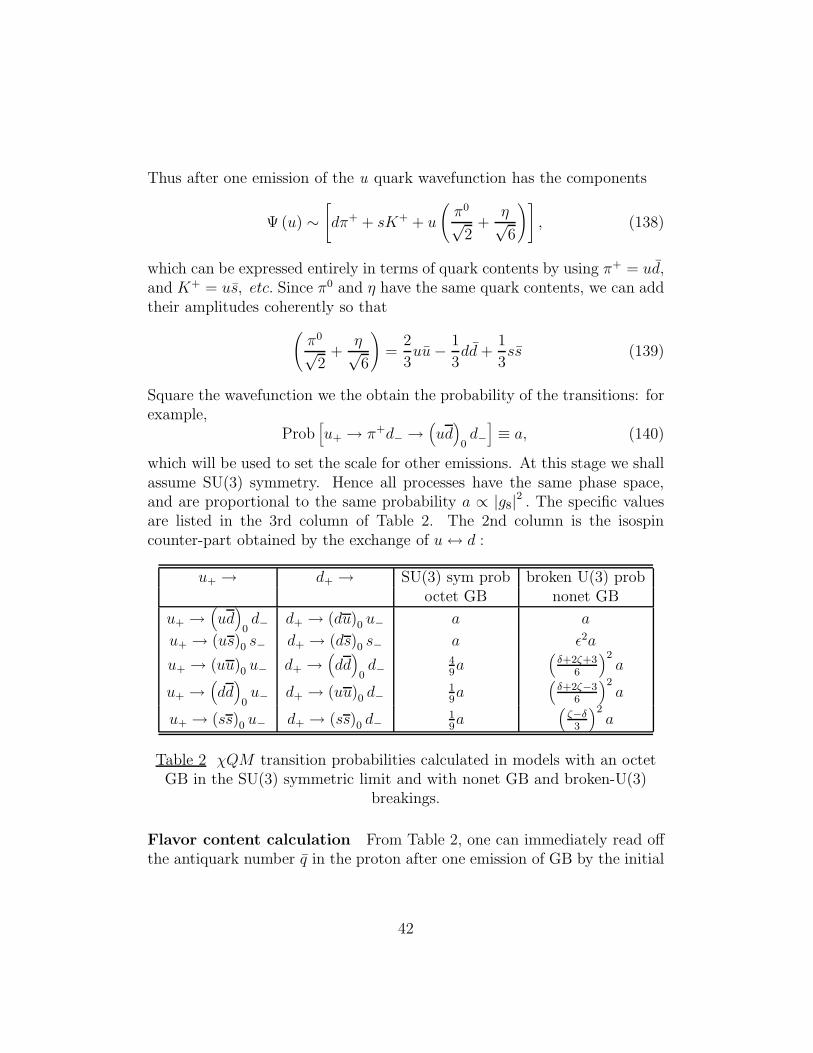
which will be used to set the scale for other emissions. At this stage we shallassume SU(3) symmetry. Hence all processes have the same phase space,and are proportional to the same probability a ∝ |g8|2 . The specific valuesare listed in the 3rd column of Table 2. The 2nd column is the isospincounter-part obtained by the exchange of u↔ d :

u+ → d+ → SU(3) sym prob broken U(3) proboctet GB nonet GB

u+ →(ud)

0d− d+ → (du)0 u− a a

u+ → (us)0 s− d+ → (ds)0 s− a ǫ2a

u+ → (uu)0 u− d+ →(dd)

0d−

49a

(δ+2ζ+3

6

)2a

u+ →(dd)

0u− d+ → (uu)0 d−

19a

(δ+2ζ−3

6

)2a

u+ → (ss)0 u− d+ → (ss)0 d−19a

(ζ−δ3

)2a

Table 2 χQM transition probabilities calculated in models with an octetGB in the SU(3) symmetric limit and with nonet GB and broken-U(3)

breakings.

Flavor content calculation From Table 2, one can immediately read offthe antiquark number q in the proton after one emission of GB by the initial

42

valence quarks (2u+ d) in the proton:

u = 2 × 4

9a+ a +

1

9a = 2a (141)

d = 2 ×(a +

1

9a)

+4

9a =

8

3a

s = 2 ×(a +

1

9a)

+(a+

1

9a)

=10

3a

Since the quark and antiquark numbers must equal in the quark sea, we havethe quark numbers in the proton:

u = 2 + u, d = 1 + d, s = s. (142)

Spin content calculation GB emission will flip the helicity of the quarkas indicated in the basic process of (136), while the quark-antiquark pairproduced through the GB channel are unpolarized:

ψ (GB) =1√2

[ψ (q+)ψ

(q′−)− ψ (q−)ψ

(q′+)]. (143)

One of the first χQM predictions about the spin structure is that, to theleading order, the antiquarks are not polarized:

∆q = q+ − q− = 0. (144)

Before GB emissions as in (136), the proton wavefunction is given by Eq.(44)giving the spin-dependent quark numbers in Eq.(45). Now from the 3rdcolumn in Table 2, we can read off the first-order probabilities:

P1 (u+ → d−) = a P1 (u+ → s−) = a P1 (u+ → u−) =2

3a, (145)

or write this in a more compact notation as

P1 (u+ →) = (d− + s− +2

3u−)a. (146)

From this we can also immediately obtain the related probabilities of P1 (u− →) ,P1 (d+ →) , and P1 (d− →) . The sum of the three terms in Eq.(145) being 8

3a,

the probability of no GB emission must then be(1 − 8

3a). Combining the

43

0th and 1st order terms of Eqs.(45) and (146), we find the spin-dependentquark densities (coefficients in front of q±):

(1 − 8

3a)(

5

3u+ +

1

3u− +

1

3d+ +

2

3d−

)+

5

3(d− + s− +

2

3u−)a

+1

3(d+ + s+ +

2

3u+)a +

1

3(u− + s− +

2

3d−)a+

2

3(u+ + s+ +

2

3d+)a

Together with Eq.(144), we can then calculate the quark polarization in theproton ∆q = ∆q + ∆q = ∆q = q+ − q− :

∆u =4

3− 37

9a, ∆d = −1

3− 2

9a, ∆s = −a. (147)

In order to account for the NMC data of Eq.(130) by u − d = −23a as in

Eq.(141), we need a probability of a ≃ 0.22. But such a large probabilitywould lead to spin content description that can at best be described as fair.For example it give a negative-valued total quark value of ∆Σ = 1−16a/3 ≃−0.17,which is clearly incompatible with the current phenomenological val-ues in Eq.(118) — although it was still marginally consistent with the originalEMC value when this calculation was first performed[40]. Also, the antiquarknumbers in Eq.(141) leads to a fixed ratio of u/d = 0.75, which is to be com-pared to the NA51 result of 0.51, as given in Eq.(133).

3.3.2 Chiral quark model with a nonet of Goldstone bosons

We have proposed[41] a broken-U(3) version of the chiral quark model withthe inclusion of the ninth GB, the η′meson.

Besides the phenomenological considerations discussed above, we havealso been motivated to modify the original χQM by the following theoreticalconsiderations. It is well-known that 1/Ncolor expansion can provide us witha useful guide to study non-perturbative QCD. In the leading 1/Ncolor expan-sion (the planar diagrams), there are nine GBs with an U(3) symmetry. Thusfrom this view point we should include the ninth GB, the η′ meson. Howeverwe also know that if we stop at this order, some essential physics would havebeen missed: At the planar diagram level there is no axial anomaly and η′

would have been a bona fide GB. Also, it has been noted by Eichten et al.[40]that an unbroken U(3) symmetry would also lead to the phenomenologicallyunsatisfactory feature of a flavor-symmetric sea: u = d = s, which clearly vi-olates the experimental results of Eqs.(130) and (133). Mathematically, this

44

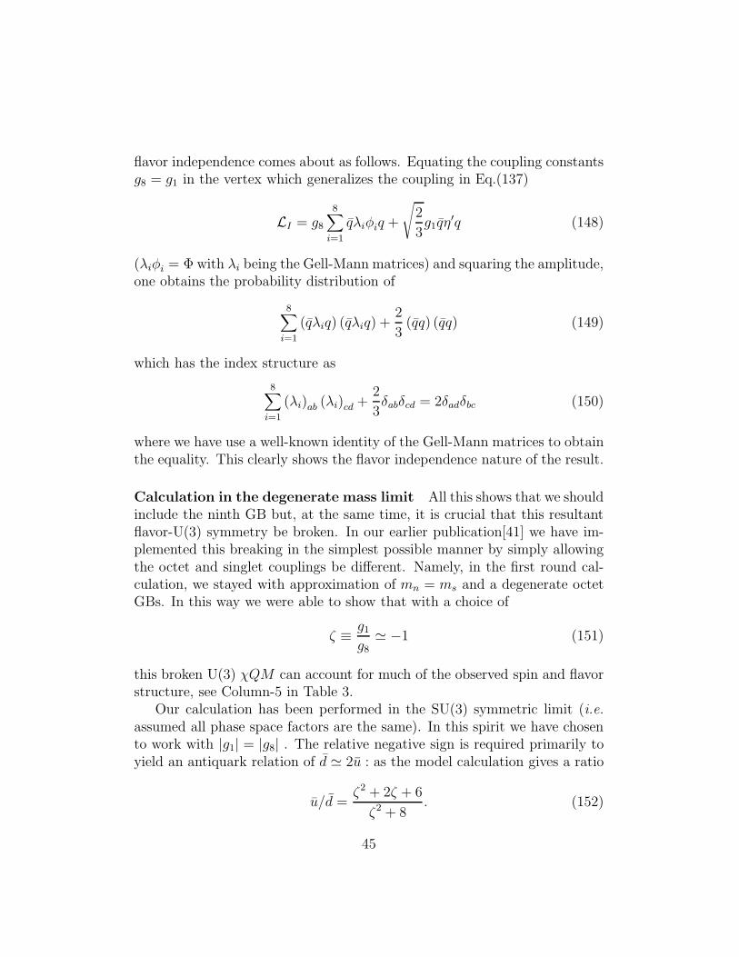
flavor independence comes about as follows. Equating the coupling constantsg8 = g1 in the vertex which generalizes the coupling in Eq.(137)

LI = g8

8∑

i=1

qλiφiq +

√2

3g1qη

′q (148)

(λiφi = Φ with λi being the Gell-Mann matrices) and squaring the amplitude,one obtains the probability distribution of

8∑

i=1

(qλiq) (qλiq) +2

3(qq) (qq) (149)

which has the index structure as

8∑

i=1

(λi)ab (λi)cd +2

3δabδcd = 2δadδbc (150)

where we have use a well-known identity of the Gell-Mann matrices to obtainthe equality. This clearly shows the flavor independence nature of the result.

Calculation in the degenerate mass limit All this shows that we shouldinclude the ninth GB but, at the same time, it is crucial that this resultantflavor-U(3) symmetry be broken. In our earlier publication[41] we have im-plemented this breaking in the simplest possible manner by simply allowingthe octet and singlet couplings be different. Namely, in the first round cal-culation, we stayed with approximation of mn = ms and a degenerate octetGBs. In this way we were able to show that with a choice of

ζ ≡ g1

g8≃ −1 (151)

this broken U(3) χQM can account for much of the observed spin and flavorstructure, see Column-5 in Table 3.

Our calculation has been performed in the SU(3) symmetric limit (i.e.assumed all phase space factors are the same). In this spirit we have chosento work with |g1| = |g8| . The relative negative sign is required primarily toyield an antiquark relation of d ≃ 2u : as the model calculation gives a ratio

u/d =ζ2 + 2ζ + 6

ζ2 + 8. (152)

45

Therefore, the experimental value of Eq.(133) implies a negative couplingratio : −4.3 < ζ < −0.7. We remark that the relative sign of the couplings isphysically relevant because of the interference effects when we coherently addthe η′ contribution to those by η and π0. After fixing this ratio, there is onlyone parameter a that we can adjust to yield a good fit. It is gratifying thata = 0.11 is indeed small, fulfilling our hope that once the singular featuresof the nonperturbative phenomenon of spontaneous symmetry breaking arecollected in the GB degrees of freedom, the remanent dynamics among theseparticles is perturbative in nature.

It should also be noted that we have compared these SU(3) symmetricresults to phenomenological values which have been extracted after usingthe SU(3) symmetry relations as well. For example the result in Eq.(118)have been extracted after using the SU(3) symmetric F/D ratio for hyperondecays as in Eq.(115). Similarly, we obtained a strange quark fraction valueF (s) ≃ 0.19 very close to that given in Eq.(79) which was deduced from σπNand an SU(3) symmetric F/D ratio for baryon masses, Eq.(77). Agreementsare in the 20% to 30% range, indicating that the broken-U(3) chiral pictureis, perhaps, on the right track.

SU(3) and axial-U(1) breaking effects The quark mass difference ms >mn, and thus the GB nondegeneracy , would affect the phase space fac-tors for various GB emission processes. Such SU(3) breaking effects willbe introduced[45][46] in the amplitudes for GB emissions, simply throughthe insertion of suppression factors: ǫ for kaons, δ for eta, and ζ for etaprime mesons, as these strange quark bearing GB’s are more massive thanthe pions. Thus the probability a ∝ |g8|2are modifies for processes involvingstrange quarks, as shown in the last column of Table 2. The suppressionfactors enter into the probabilities for u+ → (uu)0 u− and u+ →

(dd)

0u−

processes, etc. because they also receive contributions from the η and η′

GBs. Following the same steps as those in Eqs.(137) to (140), we obtain theprobabilities as listed in the 4th column of Table 2. In this way the followingresults are calculated:

u =1

12

[(2ζ + δ + 1)2 + 20

]a, (153)

d =1

12

[(2ζ + δ − 1)2 + 32

]a, (154)

s =1

3

[(ζ − δ)2 + 9ǫ2

]a. (155)

46

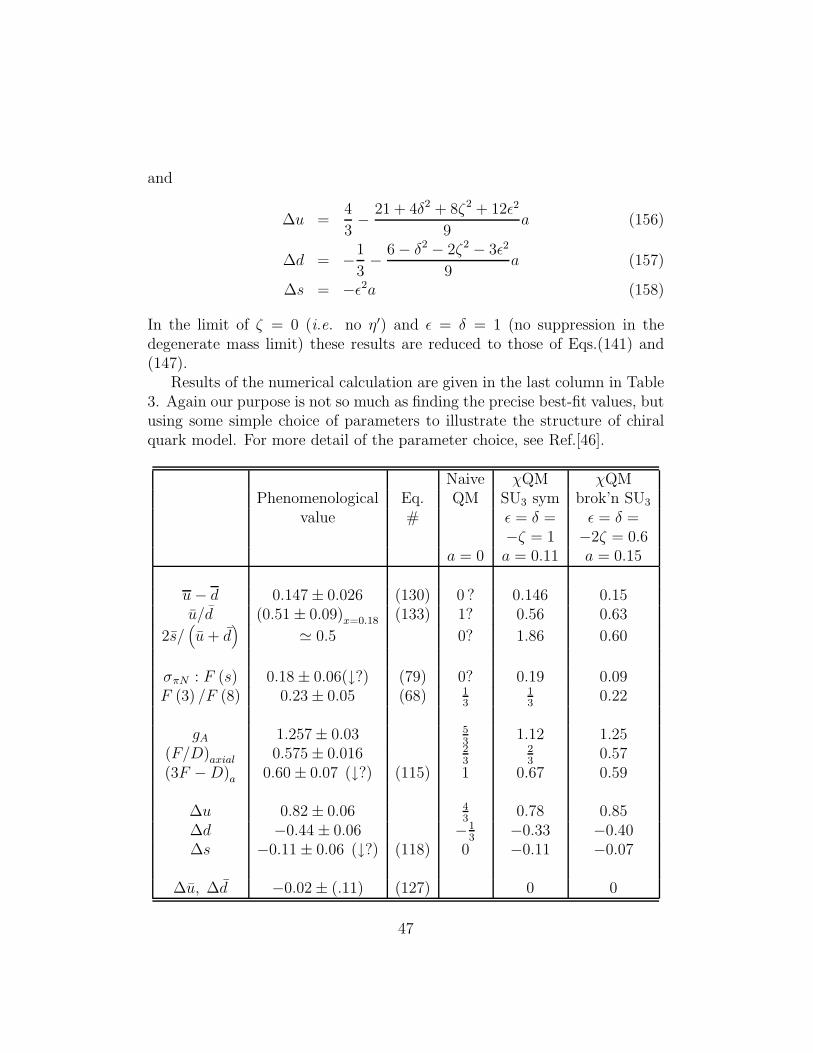
and

∆u =4

3− 21 + 4δ2 + 8ζ2 + 12ǫ2

9a (156)

∆d = −1

3− 6 − δ2 − 2ζ2 − 3ǫ2

9a (157)

∆s = −ǫ2a (158)

In the limit of ζ = 0 (i.e. no η′) and ǫ = δ = 1 (no suppression in thedegenerate mass limit) these results are reduced to those of Eqs.(141) and(147).

Results of the numerical calculation are given in the last column in Table3. Again our purpose is not so much as finding the precise best-fit values, butusing some simple choice of parameters to illustrate the structure of chiralquark model. For more detail of the parameter choice, see Ref.[46].

Naive χQM χQMPhenomenological Eq. QM SU3 sym brok’n SU3

value # ǫ = δ = ǫ = δ =−ζ = 1 −2ζ = 0.6

a = 0 a = 0.11 a = 0.15

u− d 0.147 ± 0.026 (130) 0 ? 0.146 0.15u/d (0.51 ± 0.09)x=0.18 (133) 1? 0.56 0.63

2s/(u+ d

)≃ 0.5 0? 1.86 0.60

σπN : F (s) 0.18 ± 0.06(↓?) (79) 0? 0.19 0.09F (3) /F (8) 0.23 ± 0.05 (68) 1

313

0.22

gA 1.257 ± 0.03 53

1.12 1.25(F/D)axial 0.575 ± 0.016 2

323

0.57(3F −D)a 0.60 ± 0.07 (↓?) (115) 1 0.67 0.59

∆u 0.82 ± 0.06 43

0.78 0.85∆d −0.44 ± 0.06 −1

3−0.33 −0.40

∆s −0.11 ± 0.06 (↓?) (118) 0 −0.11 −0.07

∆u, ∆d −0.02 ± (.11) (127) 0 0

47

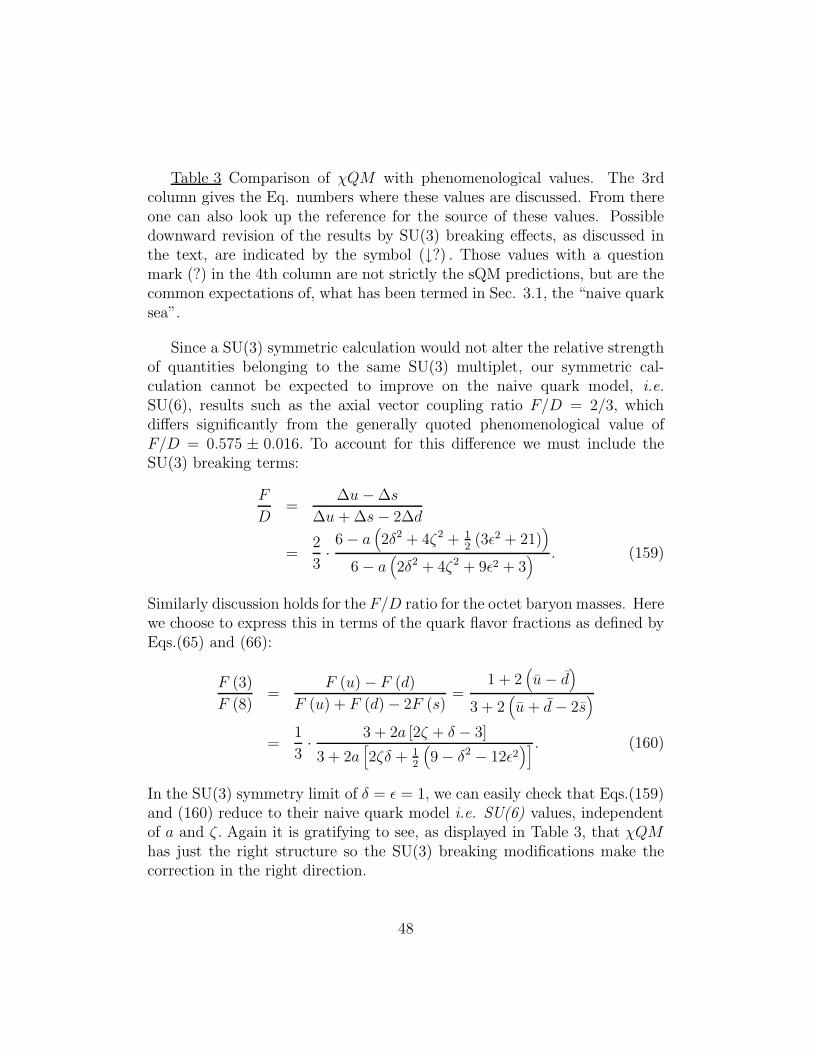
Table 3 Comparison of χQM with phenomenological values. The 3rdcolumn gives the Eq. numbers where these values are discussed. From thereone can also look up the reference for the source of these values. Possibledownward revision of the results by SU(3) breaking effects, as discussed inthe text, are indicated by the symbol (↓?) . Those values with a questionmark (?) in the 4th column are not strictly the sQM predictions, but are thecommon expectations of, what has been termed in Sec. 3.1, the “naive quarksea”.

Since a SU(3) symmetric calculation would not alter the relative strengthof quantities belonging to the same SU(3) multiplet, our symmetric cal-culation cannot be expected to improve on the naive quark model, i.e.SU(6), results such as the axial vector coupling ratio F/D = 2/3, whichdiffers significantly from the generally quoted phenomenological value ofF/D = 0.575 ± 0.016. To account for this difference we must include theSU(3) breaking terms:

F

D=

∆u− ∆s

∆u+ ∆s− 2∆d

=2

3·6 − a

(2δ2 + 4ζ2 + 1

2(3ǫ2 + 21)

)

6 − a(2δ2 + 4ζ2 + 9ǫ2 + 3

) . (159)

Similarly discussion holds for the F/D ratio for the octet baryon masses. Herewe choose to express this in terms of the quark flavor fractions as defined byEqs.(65) and (66):

F (3)

F (8)=

F (u) − F (d)

F (u) + F (d) − 2F (s)=

1 + 2(u− d

)

3 + 2(u+ d− 2s

)

=1

3· 3 + 2a [2ζ + δ − 3]

3 + 2a[2ζδ + 1

2

(9 − δ2 − 12ǫ2

)] . (160)

In the SU(3) symmetry limit of δ = ǫ = 1, we can easily check that Eqs.(159)and (160) reduce to their naive quark model i.e. SU(6) values, independentof a and ζ. Again it is gratifying to see, as displayed in Table 3, that χQMhas just the right structure so the SU(3) breaking modifications make thecorrection in the right direction.

48

3.4 Strange quark content of the nucleon

We have already discussed the number s of strange quarks in the nucleonquark sea and their polarization ∆s. They are examples of the proton matrixelements of operators bilinear in the strange quark fields 〈p |sΓis| p〉 , or ingeneral we need to study the quark bilinear matrix elements of 〈p |qΓiq| p〉 :

3.4.1 The scalar channel

This operator counts the number of quarks plus the number of antiquarksin the proton. In particular the octet components of

⟨p∣∣∣uu− dd

∣∣∣ p⟩

and⟨p∣∣∣uu+ dd− 2ss

∣∣∣ p⟩

can be gotten by SU(3) baryon mass relations as we

have shown in Eq.(66). But in order to separate out the individual terms, say

〈p |ss| p〉, we would need the singlet combination⟨p∣∣∣uu+ dd+ ss

∣∣∣ p⟩. This is

provided by σπN which is a linear combination of the singlet and octet pieces.That is why a measurement of σπN allows us to do an SU(3) symmetriccalculation of the strange quark content of the nucleon.

We have emphasized that OZI violation means that the couplings for sspair creation and annihilation may not be suppressed even though the phasespace surely does not favor such processes. But the phase space suppressionis a “trivial” SU(3) breaking effect. Our chiral quark model calculation is aconcrete realization of this possibility: Had we ignored the phase space dif-ference, the GB-quark couplings are such that there would be more strangequark pairs than either of the nonstrange pairs in the quark sea, as ss pro-duction by either u or d valence quarks are not disfavored. Thus Eq.(141)give a relative quark abundance in the quark sea of

u : d : s = 3 : 4 : 5 (161)

In the physical quark sea we do not really expect strange quark pairs todominate because of their production is suppressed by SU(3) breaking effects.

The χQM naturally suggests that the nucleon strange quark content s andpolarization ∆s magnitude are lowered by the SU(3) breaking effects as theyare directly proportional to the amplitude suppression factors, see Eqs.(155)and (158). This is just the trend found in the extracted phenomenologicalvalues. Gasser[47], for instance, using a chiral loop model to calculate theSU(3) breaking correction to the Gell-Mann-Okubo baryon mass formula,finds that the no-strange-quark limit-value of (σπN )0 is modified from 25 to35MeV, [i.e. the baryon mass M8 in Eq.(77) changed from −200 by SU(3)

49

breakings to −280MeV ], thus the fraction F (s) from 0.18 to 0.10. It matchesclosely our numerical calculation with the illustrative parameters, see Table3.

The strange quark content can also be expressed as the relative abundanceof the strange to non-strange quarks in the sea, which in this model is givenas

λs ≡s

12

(u+ d

) = 4(ζ − δ)2 + 9ǫ2

(2ζ + δ)2 + 27≃ 1.6ǫ2 = 0.6. (162)

This can be compared to the strange quark content as measured by the CCFRCollaboration in their neutrino charm production experiment[48]

κ ≡ 〈xs〉12

(〈xu〉 +

⟨xd⟩) = 0.477±0.063, where 〈xq〉 =

∫ 1

0xq (x) dx, (163)

which is often used in the global QCD reconstruction of parton distributions[49].The same experiment found no significant difference in the shapes of thestrange and non-strange quark distributions[48]:

[xs (x)] ∝ (1 − x)α[xu (x) + xd (x)

2

],

with the shape parameter being consistent with zero, α = −0.02±0.08. Thus,it is reasonable to use the CCFR findings to yield

λs ≃ κ ≃ 1

2, (164)

which is a bit less than, but still compatible with, the value in Eq.(162).Thus it is seen that the χQM can yield a consistent account of the strange

quark content s of the proton sea. SU(3) breaking is the key in reconciling thes value as measured in the neutrino charm production and that as deducedfrom the pion nucleon sigma term.

3.4.2 The axial-vector channel

This operator measures the quark contribution to the proton spin. In par-ticular the octet components of

⟨p, s

∣∣∣uγµγ5u− dγµγ5d∣∣∣ p, s

⟩

50

and ⟨p, s

∣∣∣uγµγ5u+ dγµγ5d− 2sγµγ5s∣∣∣ p, s

⟩

can be gotten by SU(3) relations among the axial vector couplings of octetbaryon weak decays, Eqs.(114) and (115). But in order to separate out the

individual terms, say⟨p, s

∣∣∣sγµγ5s∣∣∣ p, s

⟩= 2sµ∆s, we would need the singlet

combination ∆u + ∆d + ∆s. This is provided by the first-moment of thestructure function

∫g1dx which is a linear combination of the singlet and

octet pieces. That is why a measurement of g1 (x) allows us to do an SU(3)symmetric calculation of the strange quark content of the nucleon.

A number of authors have pointed out that phenomenologically extractedvalue of strange quark polarization ∆s is sensitive to possible SU(3) breakingcorrections. While the effect is model-dependent, various investigations[42] -[44] all conclude that SU(3) breaking correction tends to lower the magnitudeof ∆s. Some even suggested the possibility of ∆s ≃ 0 being consistent withexperimental data. Our calculation indicates that, while ∆s may be smallerthan 0.10, it is not likely to be significantly smaller than 0.05. To verify thisprediction, it is then important to pursue other phenomenological methodsthat allow the extraction of ∆s without the need of SU(3) relations.

Besides polarized DIS of charged lepton off nucleon, we can also use otherprocesses to determine ∆s. In elastic neutrino-proton scattering, we can sep-arate out the axial form factors at zero momentum transfer,

⟨p′∣∣∣qγµγ5q

∣∣∣ p⟩

= 2u (p′)

[G

(q)1

(Q2)γµγ5 +

qµγ5

2MpG

(q)2

(Q2)]u (p) . (165)

Thus we have G(q)1 (0) = ∆q. The axial vector matrix element arises from

Z-boson exchange is proportion to

⟨p′∣∣∣qT3γµγ5q

∣∣∣ p⟩

=1

2

⟨p′∣∣∣uγµγ5u− dγµγ5d− sγµγ5s

∣∣∣ p⟩

(166)

where T3 is the 3rd component of the weak isospin operator. The⟨p∣∣∣sγµγ5s

∣∣∣ p⟩

can be separated out because the first two terms are fixed by the neutronaxial coupling gA. Present data still have large error, however they are con-sistent with a ∆s 6= 0[50].

The measurements of longitudinal polarization of Λ in the semi-inclusiveprocess of νN → µΛ +X [51] have also given support to a nonvanishing andnegative ∆s. In this connection, it’s also important to pursue experimen-tal measurements to check the χQM prediction for a vanishing longitudinal

51

polarization of Λ in the semi-inclusive processes reflecting the proton spinproperty of ∆s = 0.

3.4.3 The pseudoscalar channel

The nucleon matrix elements of the pseudoscalar quark density may be phys-ically relevant in Higgs coupling to the nucleon[52], etc. Such operators maybe related to the axial vector current operator through the (anomalous) di-vergence equation (121)[53]. If we define

〈p |qiγ5q| p〉 = νqu (p) iγ5u (p) (167)⟨p∣∣∣trGµνGµν

∣∣∣ p⟩

= −∆g2Mpu (p) iγ5u (p) (168)

so that the non-strange divergence equations may be written as

2Mp∆u = 2muνu − 2Mp

(αs2π

∆g)

(169)

2Mp∆d = 2mdνd − 2Mp

(αs2π

∆g)

We would need one more condition in order to separate out the individualmqνq terms. This may be obtained by saturation of the nonsinglet channel byGoldstone poles. Let us recall that the Goldberger-Treiman relation can bederived in the charge channel by the π± pole-dominance of the pseudoscalardensity. After taking the nucleon matrix element of

∂µ(uγµγ5d

)= (mu +md) (uiγ5d)

one obtains2MpgA = 2fπgπNN + µ± (170)

where µ± denotes the correction to the π± pole-dominance, and is the cor-rection to the gA as given by the GT relation. Repeating the same for theneutral isovector channel

∂µ(uγµγ5u− dγµγ5d

)= 2mu (uiγ5u) − 2md

(diγ5d

)

we have2MpgA = 2fπgπNN + µ0 + (mu −md) (νu + νd) (171)

Comparing these two expressions for gA one concludes that the singlet den-sity (νu + νd) must be small, on the order of correction to the GT expression

52

of gA. Assume that µ0 ≃ µ±, thus νu = −νd, we can solve the two equationsin (169) in terms of the measured ∆u and ∆d given in Eq.(118).

muνu = 423MeV mdνd = −761MeVαs2π

∆g = −0.37. (172)

With these values we can also obtain

msνs = −451MeV . (173)

Because of the large strange quark masses ms, this translates into fairly smallstrange pseudoscalar matrix element of

〈p |siγ5s| p〉 ≃ 0.03⟨p∣∣∣diγ5d

∣∣∣ p⟩.

3.4.4 The vector channel

Of course the vector charges

Qi =∫d3xV i

0 (x) with V iµ = qγµ

λi

2q (174)

are simply the generators of the flavor SU(3). In terms of the form factorsdefined as

⟨p′∣∣∣∣∣qγµ

λi

2q

∣∣∣∣∣ p⟩

= u (p)

[γµF

(q)1

(Q2)

+ iσµν (p′ − p)ν

2MpF

(q)2

(Q2)]u (p)

(175)

whereQ2 = (p′ − p)2 is the momentum transfer, we note that⟨p∣∣∣qγµ

λi

2q∣∣∣ p⟩∣∣∣Q2=0

are constrained by the quantum numbers of the proton:

F(u)1 (0) − F

(d)1 (0) = 1, F

(s)1 (0) = 0. (176)

However, the magnetic moment form factor F(s)2 (0) needs not vanish. It

is therefore interesting to measure this quantity. This can be done throughthe observation of parity violation in the scattering of charged-leptons offnucleon. The interference of the photon-exchange and Z-boson-exchange dia-grams can be used to isolate F

(s)2 (0). For detailed discussion, see Refs.[54][55].

53

3.5 Discussion

In these lectures we have described an attempt to understand the nucleonspin-flavor structure in the framework of a broken-U(3) chiral quark model.The broad agreement obtained with simple schematic calculations, as dis-played in Table 3, has been quite encouraging. If this approach turns outto be right, it just means that the familiar non-relativistic constituent quarkmodel is basically correct — it only needs to be supplemented by a quarksea generated by the valence quarks through their internal GB emissions.

Because the couplings between GB and constituent quarks are not strong,we can again use perturbation theory based on these non-perturbative de-grees of freedom — even though the phenomena we are describing are non-perturbative in terms of QCD Lagrangian quarks and gluons. Features suchas d ≃ 2u are seen to be clear examples of nonperturbative QCD physics, asthey are quite inexplicable in terms of a quark sea generated by perturbativegluon emissions. (If one gets beyond the perturbative gluonic picture, thisd 6= u property is not peculiar at all, as the nucleon is not an isospin sin-glet and there is no reason to expect that its quark sea should be an isospinsinglet.)

In the case of the proton spin structure, because the most often discussedtheoretical interpretation is the possibility of a hidden gluonic contribution,it has led some to think that other approaches, such as χQM, must beirrelevant. But the alternative theories are attempting a different descriptionby using different degrees of freedom. To be sure, the QCD quarks and gluonsare the most fundamental DOF. But we cannot insist on using them for suchnon-perturbative problems as the hadron structure. An analogy with thenucleon mass problem will illustrate our point.

The canonical approach to study the various quarks/gluon contributionsto the nucleon mass is through the energy-momentum trace anomaly equation[56]:

Θµµ = muuu+mddd+msss−

(11 − 2

3nf

)αs8πtrGµνGµν . (177)

Just like the more familiar axial vector anomaly equation, the naive diver-gence is given by quark masses while the anomaly term is given by the gluonfield tensor. (Of course, here we are using the Lagrangian quark and gluonfields.) When taken between the proton states, this equations yields

Mp = mn

⟨p∣∣∣uu+ dd

∣∣∣ p⟩

+ms 〈p |ss| p〉 + gluon term (178)

54

The first term is just the σπN ≃ 45MeV representing a tiny contribution bythe nonstrange quarks, while the second term can also be estimated[52]:

ms 〈p |ss| p〉 =msσπN2mn

[1 − 3mn

mn −ms

M8

σπN

]≃ 250MeV. (179)

[Because this is an SU(3) calculation, the strange quark term is somewhatoverestimated.] One way or other, we see that most of the proton mass camefrom the gluon term[57]. Heavy quark terms can also be included but theircontributions as explicit quark terms just cancel the corresponding heavyquark loops in the gluon terms. In this sense they decouple[58].

This led to an important insight: nucleon mass is mostly gluonic. Butin terms of the QCD quarks and gluons, it is difficult to say anything more.That is why the description provided by the constituent quark model is soimportant. In this picture much more details can be constructed: hyperfinesplitting, magnetic moments, etc.

The important point is that these two approaches are not mutually ex-clusive. While the constituent quark model does not refer explicitly to gluon,the above discussion suggests that it is the non-perturbative gluonic inter-action that brings about the large constituent quark masses. (In the χQMthis takes the form of quark interaction with the chiral condensate of theQCD vacuum.) We believe that this complimentarity of the QCD and sQMdescriptions holds for the flavor-spin structure problem as well. The non-perturbative features can be described much more succinctly if we use thenon-perturbative DOF of constituent quarks and internal GBs. Thus it isquite possible that the statement of a significant gluonic contribution to theproton spin and a correct description of spin structure by the χQM can bothbe valid — just the same physics expressed in two different languages.

Acknowledgment

L.F.L. would like to thank the organizers, in particular C.B. Lang, of theSchladming Winter School for warm hospitality. His work is supported atCMU by the U.S. Department of Energy (Grant No. DOE-ER/40682-127).

55

References

[1] T.P. Cheng and L.F. Li, Gauge Theory of Elementary Particle Physics,Clarendon Press, Oxford, 1984. Ch.5.

[2] M. Gell-Mann, R. Oaks, and B. Renner, Phys. Rev. 175, 2195 (1968).

[3] R. Dashen, Phys. Rev. 183, 1291 (1969).

[4] S. Coleman and H. Schnitzer, Phys. Rev. 136, B223 (1964).

[5] A. DeRujula, H. Georgi, and S.L. Glashow, Phys. Rev. D 12, 147 (1975).

[6] J. Rosner, Proc. Adv. Study Inst. on Tech. and Concepts in High EnergyPhysics, St. Croix, USVI, ed. T. Ferbel (1980).

[7] S. Okubo, Phys. Lett. 5, 163 (1963); G. Zweig, CERN Report No.8419/TH 412 (1964); J. Iizuka, Prog. Theor. Phys. Suppl. 37-8, 21(1966).

[8] T. Appelquist and H.D. Politzer, Phys. Rev. Lett. 34, 43 (1975).

[9] T.P. Cheng and R.F. Dashen, Phys. Rev. Lett. 26, 594 (1971).

[10] T.P. Cheng, Phys. Rev. D 13, 2161 (1976).

[11] J. Gasser, H. Leutwyler, and M.E. Sainio, Phys. Lett. B253, 252 (1991).

[12] H.Y. Cheng, Int. J. Mod. Phys. A, 11, 5109 (1996).

[13] A.V. Manohar, in Proc. 7th Lake Louis Winter Institute (1992), eds.B.A. Campbell et al. (World Scientific, Singapore, 1992).

[14] J. Kodaira et al., Phys. Rev. D 20, 627 (1979); S.A. Larin, F. V.Tkachev, and J.A.M. Vermaseren, Phys. Rev. Lett. 66, 862 (1991).

[15] For a review see, e.g. Ref. [1], Ch.10.

[16] For a review see, e.g. Ref. [1], Ch.7.

[17] S.Y. Hsueh et al. Phys. Rev. D 38, 2056 (1988); F.E. Close and R.G.Roberts, Phys. Lett. B341, 165 (1993).

56

[18] S.A. Larin, Phys. Lett. B334, 192 (1994); A.L. Kataev and V.Starshenko, Mod. Phys. Lett. A 10, 235 (1995).

[19] J. Ellis and R.L. Jaffe, Phys. Rev. D 9, 1444 (1974).

[20] E80 Collaboration, M.J. Alguard et al., Phys. Rev. Lett. 37, 1261(1976);Phys. Rev. Lett. 41, 70 (1978);G. Baum et al., Phys. Rev. Lett.45, 2000 (1980).

[21] European Muon Collaboration, J. Ashman, et al., Phys. Lett. B206,364 (l988); Nucl. Phys. B328, 1 (1990).

[22] Spin Muon Collaboration, B. Adeva et al., Phys. Lett. B302, 533 (1993);D. Adams et al., Phys. Lett. B329, 399 (1994); B339, 332(E) (1994);B357, 248 (1995).

[23] E142 Collaboration, P. L. Anthony et al., Phys. Rev. Lett. 71, 959(1993). E143 Collaboration, K. Abe et al. Phys. Rev. Lett. 74, 346(1995); Phys. Rev. Lett. 75, 25 (1995).

[24] J. Ellis and M. Karliner, Phys. Lett. B341, 397 (1995).

[25] A.V. Efremov and O.V. Teryaev, JINR Report E2-88-287 (1988), G.Altarelli and G.G. Ross, Phys. Lett. B212, 391 (1988); R.D. Carlitz,J.C. Collins and A.H. Mueller, Phys. Lett. B214, 229 (1988); see also,C.S. Lam and B.N. Li, Phys. Rev. D 25, 683 (1982).

[26] Spin Muon Collaboration, B. Adeva et al., Phys. Lett. B369, 93 (1996).

[27] G. Karl, Phys. Rev. D 45, 247 (1992).

[28] T.P. Cheng and L.-F. Li, Phys. Lett. B366, 365; (E) B381, 487 (1996).

[29] K. Gottfried, Phys. Rev. Lett. 18, 1174 (1967).

[30] New Muon Collaboration, P. Amaudruz et al. Phys. Rev. Lett. 66, 2712(1991); M. Arneodo et al. Phys. Rev. D 50, R1 (1994).

[31] S.D. Ellis and W.J. Stirling, Phys. Lett. B256, 258 (1993).

[32] NA 51 Collaboration, A. Baldit et al. Phys. Lett. B332, 244 (1994).

57

[33] F.E. Close, An Introduction to Quarks and Partons, Academic Press,London (1979). For a recent discussion of the quark model (without theGoldstone structure) with respect to the Q2 6= 0 probes of the nucleonspin content, see F. Close, Talk at the 6th ICTP Workshop, Trieste(1993), Rutherford Appleton Lab Report RAL-93-034.

[34] R.D. Field and R.P. Feynman, Phys. Rev. D 15, 2590 (1977).

[35] See, e.g., E.M. Henley and G.M. Miller, Phys. Lett. B251, 453 (1990).

[36] J.D. Sullivan, Phys. Rev. D 5, 1732 (1972).

[37] A. Manohar and H. Georgi, Nucl. Phys. B234, 189 (1984); S. Weinberg,Physica (Amsterdam) 96A, 327 (1979), Sec. 6; H. Georgi, Weak Interac-tions and Modern Particle Theory, (Benjamin/Cummings, Menlo Park,CA, 1984), Sec. 6.4 and 6.5.

[38] L. Ya. Glozman and D. O. Riska, Phys. Rept. 268, 263 (1996); L. Ya.Glozman, in “Perturbative and Non-perturbative Aspects of QuantumField Theory” Proc. 1996 Schladming Lectures, Springer-Verlag (Berlin,Heidelberg) 1996.

[39] J. D. Bjorken, in “Proc 4th Int. Conf. on Elastic and Diffractive Scat-terings - 1991”, published in Nucl. Phys. Proc. Suppl. 25B, 253 (1992).

[40] E.J. Eichten, I. Hinchliffe, and C. Quigg, Phys. Rev. D 45, 2269 (1992).

[41] T.P. Cheng and L.-F. Li, Phys. Rev. Lett. 74, 2872 (1995).

[42] B. Ehrnsperger, and A. Schafer, Phys. Lett. B348, 619 (1995).

[43] J. Lichtenstadt and H. J. Lipkin, Phys. Lett. B353, 119 (1995).

[44] J. Dai, R. Dashen, E. Jenkins, and A. Manohar, Phys. Rev. D 53, 273(1996).

[45] X. Song, J.S. McCarthy, and H.J. Weber, Phys. Rev. D 55, 2624 (1997).

[46] T.P. Cheng and L.-F. Li, CMU-HEP97-01, hep-ph/9701248, submittedfor publication in Phys. Rev. D.

[47] J. Gasser, Ann. Phys. (NY) 136, 62 (1981).

58

[48] CCFR Collaboration, A. O. Bazarko, et al., Z. Phys. C 65, 189 (1995).

[49] A.D. Martin, W.J. Stirling, and R.G. Roberts, Phys. Rev. D 50, 6734(1994); CTEQ Collaboration, H. L. Lai, et al., Phys. Rev. D 51, 4763(1995).

[50] D.B. Kaplan and A.V. Manohar, Nucl. Phys. B310, 527 (1988).

[51] WA58 Collaboration, S. Willocq et al., Z. Phys. C 53, 207 (1992); J.Ellis, D. Kharzeev, and A. Kotzinian, Z. Phys. C 69, 467 (1996).

[52] T.P. Cheng, Phys. Rev. D 38, 2869 (1988).

[53] T.P. Cheng and L.-F. Li, Phys. Rev. Lett. 62, 1441 (1989).

[54] R.D. McKeown, Phys. Lett. B219, 140 (1989); D.H. Beck, Phys. Rev.D 39, 3248 (1989).

[55] B. Mueller et al., Phys. Rev. Lett. 78, 3824 (1997).

[56] R. Crewther, Phys. Rev. Lett. 28, 1421 (1972); M. Chanowitz and J.Ellis, Phys. Lett. B40, 397 (1972); S.L. Adler, J.C. Collins, and A.Duncan, Phys. Rev. D 15, 1712 (1977).

[57] M.A. Shifman, A.I. Vainstein, and V.I. Zakharov, Phys. Lett. B78, 443(1978).

[58] T.P. Cheng and L.-F. Li, “Proc. the Rice Meeting – DPF’90”, eds. B.Bonner and H. Miettienen, World Scientific (Singapore, 1990), p569.

59