8

The Pros and Cons of Predicting Protein Contact Maps

Lisa Bartoli, Emidio Capriotti, Piero Fariselli, Pier Luigi Martelli,and Rita Casadio

SummaryIs there any reason why we should predict contact maps (CMs)? The question is one of the

several ‘NP-hard’ questions that arise when striving for feasible solutions of the protein foldingproblem. At some point, theoreticians started thinking that a possible alternative to an unsolvableproblem was to predict a simplified version of the protein structure: a CM. In this chapter, wewill clarify that whenever problems are difficult they remain at least as difficult in the processof finding approximate solutions or heuristic approaches. However, humans rarely give up, as itis stimulating to find solutions in the face of difficulties. CMs of proteins are an interesting anduseful representation of protein structures. These two-dimensional representations capture all theimportant features of a protein fold. We will review the general characteristics of CMs and themethods developed to study and predict them, and we will highlight some new ideas on how toimprove CM predictions.

Key Words: Protein structure prediction; Protein contacts; Small world; Structure recon-struction; Machine learning; Contact map; Protein folding.

1. From Protein Structures to Contact MapsProteins structures are described by the coordinates (CO-representation) of

the atoms that constitute the macromolecule. For a protein with n atoms weneed 3n numbers (x, y and z coordinates for each atom) to specify its three-dimensional (3D) structure. An alternative view is to consider the distancematrix (DM), a symmetric matrix that contains the Euclidean distance betweeneach pair of atoms. If the number of atoms is n we need n2 elements; because

From: Methods in Molecular Biology, vol. 413: Protein Structure Prediction, Second EditionEdited by: M. Zaki and C. Bystroff © Humana Press Inc., Totowa, NJ

199

200 Bartoli et al.

the matrix is symmetric (the distance between atoms i and j is the same ofthat between j and i), the real number of elements is only n(n – 1)/2. Bothrepresentations, namely the coordinates and the DM, are equivalent, that is, wecan convert each representation into the other. DM can be computed from theCO-representation simply by evaluating the Euclidean distance between eachpair of atoms: values stored in the appropriate DM cell uniquely identify thepair i and j. Conversely, to go from DM to CO is not so trivial. There exists aLagrange theorem (1) that states that once that the Gram matrix derived fromDM is diagonalized, the three eigenvectors that correspond to the three highesteigenvalues are the atom coordinates in a 3D cartesian reference. Actually,there are two solutions, but the chirality of the molecule routinely can help inselecting the correct one (1 and references therein).

DM representation has far more elements than the coordinate-based represen-tation, so why adopt it? The main advantage of DM representation arises whenonly a part of the data is known (i.e., in low-resolution NMR experiments). Stillsolutions can be found, thanks to DM properties (1). Another advantage of DMis that the protein is represented in a framework that automatically incorporatestranslational and rotational invariance and this in principle is more suitable forlearning approaches.

Quite often in order to simplify the protein representation not all proteinatoms are taken into account and residues are considered as unique entities.In this case, the DM has a number of rows (and columns) equal to theresidue numbers. Each DM entry is then the distance between residue i and j.The distance between two residues can be defined in different ways, suchas the following:

• the distance between a specific pair of atoms (i.e., CA–CA or CB–CB),• the shortest distance among the atoms belonging to i residue and those belonging toresidue j, and

• the distance between the centres of mass of the two residues.

Even though these choices are quite different and structurally minimal, theyprovide enough information to build the protein backbone, or at least the CAtrace (1,2).

Starting from the protein DM and selecting an arbitrary distance cut-off,a further simplified representation can be obtained: the protein contact map(CM). CMs are binary symmetric matrices, whose non-zero elements represent

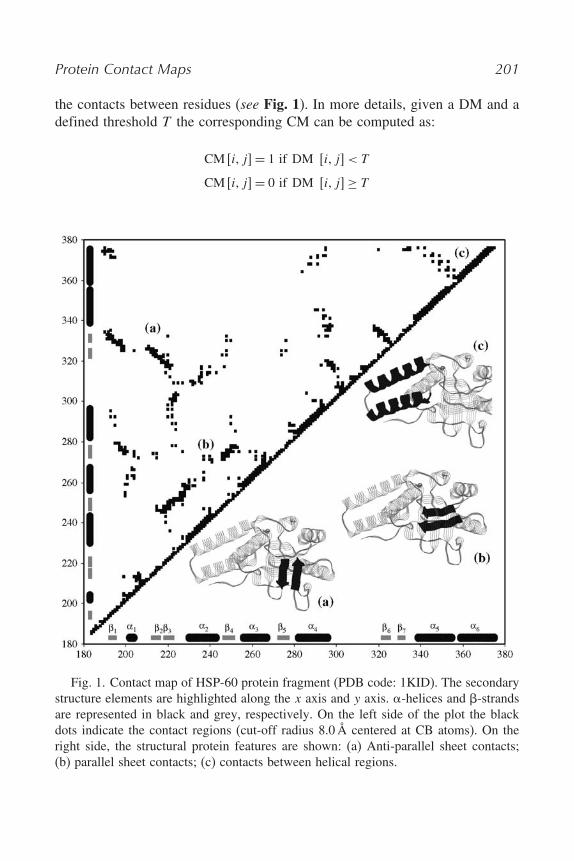
Protein Contact Maps 201

the contacts between residues (see Fig. 1). In more details, given a DM and adefined threshold T the corresponding CM can be computed as:

CM !i" j#= 1 if DM !i" j#< T

CM !i" j#= 0 if DM !i" j#! T

Fig. 1. Contact map of HSP-60 protein fragment (PDB code: 1KID). The secondarystructure elements are highlighted along the x axis and y axis. $-helices and %-strandsare represented in black and grey, respectively. On the left side of the plot the blackdots indicate the contact regions (cut-off radius 8.0Å centered at CB atoms). On theright side, the structural protein features are shown: (a) Anti-parallel sheet contacts;(b) parallel sheet contacts; (c) contacts between helical regions.

202 Bartoli et al.

While the problem of reconstructing the protein coordinates from the DMhas a well known solution, there are no analogous theorems for CM. However,some empirical applications have been built to address this issue. The resultsindicate that (at least for the tested proteins) it is possible to reconstruct theCO-representations from CMs (2–5).

Protein CM representation has some pros and cons.Pros:

• Unlike other protein representations such as secondary structure, CM conveys stronginformation about the protein 3D structure.

• The CM representation is translation and rotation invariant and more compact thanthe DM representation.

• CM is more suited than DM for learning problems. The binary CM nature canbe regarded as a classical problem of a two-state classification and this hasbeen thoroughly studied. There are several machine learning methods availableto address the problem of the prediction of CM from the protein residuesequence (6).

• It has been shown that the empirical reconstruction algorithms are quite insensitiveto high levels of random noise in CMs, so that for reconstructing the 3D structureof the protein it is not necessary to correctly predict all contacts (2,4).

Cons:

• There is no theory on CM that can help to define the limits and the strength of thisrepresentation. For instance, the effect of the contact threshold on the informationcontent is not theoretically assessable. For this reason, different researchers adoptdifferent protein representations and contact thresholds.

• The problem of CM comparison is very hard, as it is that of a sub-graph isomorphism,which is NP-hard (7).

• CMs of real proteins are a tiny subset of the possible binary symmetric matrices (2);however, no simple and fast algorithm has been found to sort out the protein-feasibleCM from the others.

• CM prediction is an intrinsically non-local problem. Also, this is a very difficultproblem to deal with, as a contact between two residues poses constraints on thefeasibilities of all other contacts.

• Although the reconstruction programs are very insensitive to random noise, they arenot as robust when the prediction errors are correlated, as is the case with currentprediction algorithms.

CMs can be regarded both as symmetric matrices and as graphs. Actually,the CM representation is an adjacency matrix, where the contacts are theedges and the residues are the nodes. It is useful to distinguish betweenshort-range and long-range contacts. The distinction between short-range

Protein Contact Maps 203

(sometimes called ‘local’) and long-range (‘non-local’) contacts is not dueto the type of interaction, nor the spatial distance, but it is due to therelative sequence separation. Contacts between residues that are separated lessthan a given number of residues S &"i# j" $ S' are said to be short-range.Conversely, if the sequence separation is greater than S, they are said to belong-range. The choice of S is arbitrary, but it is commonly accepted that"i# j" $7#10 represents short-range contacts, while "i# j" >7#10 representslong-range ones.

2. Properties of Protein Contact MapsWhen CMs are analyzed, one of the first features is that the number of

contacts increases almost linearly with the protein length, independently of theadopted distance measures (CA–CA, CB–CB, etc.) and of the threshold cut-offused (8). More formally, if L is the protein length and nc is the number ofcontacts, the real number of contacts can be quite accurately estimated usingthe linear equation

nc = AT %L

where AT is a constant that only depends on the contact threshold (T ). Inpractice, a change in the contact threshold T (in a reasonable range) has the onlyeffect of modifying the slope of the line. This finding, together with the factthat the number of possible contacts NCM, which is the number of independentCM elements &NCM = L&L#1'/2', increases with the square of the proteinlength, implies that the contact densities in the map &nc/NCM' decrease asthe inverse of the protein length. In other words, long proteins have a lowercontact density than short ones (8).

Protein CMs have also more contacts in the short-sequence separations thanthose obtained using random graphs with the same number of contacts (8). Thisis an indication that protein structures have a high tendency to form contactswith sequence neighbours.

Studying the properties of the CM eigenvectors, it has been found that thereis a high correlation between the eigenvector corresponding to the highesteigenvalue (first eigenvector) and the residue coordination numbers (5,9). Theresidue coordination number (or contact vector) is the number of contacts ofeach given residue with all the others in the protein space (10). This figure canbe easily computed from the contact matrix by summing up the rows (or thecolumns) of CM.

204 Bartoli et al.

Galaktionov and Marshall (5) reported that from the knowledge of the realresidue coordination numbers, it is possible to reconstruct to some extent (about4Å of Root Mean Square Deviation (RMSD)) the 3D structure of the protein.

A further surprising property of the first eigenvector of CM is the factthat a CM can be reconstructed using only the information contained in thisvector coupled along with the information derived from the protein backboneconstraints (9). However, this is not a general property of all binary symmetricmatrices, only of the subset comprising single-domain proteins (9).

3. Reconstructing Protein Structures From Contact MapsAs outlined above, a CM contains a simplified representation of the protein

conformation and it is unambiguously computed from the structure by a binarysimplification of the DM. It is well known that a protein structure can be recon-structed from its DM by means of the Lagrange theorem (1). This procedure isunambiguous, except for the ambiguity due to chiral symmetry. The questionsare these: is it possible to recover the structure starting from its real CM aswell? And from a predicted CM?

Bohr et al. (3) implemented a method based on the definition of a continuousfunction that measures the distance of a protein structure from a given CM. Byadding some terms for assuring the connectivity and the compactness of theprotein structure, a target function was obtained and then minimized using asimple steepest descent algorithm. The optimal computed structure satisfies asmany contacts as possible.

At an 8Å threshold for the distance between two CA atoms, the algorithmrecovers the structure starting from the real CM with a RMSD less than 3Å.It is worth noticing that the threshold value for the contact definition canbe chosen within a wide range without greatly affecting the deviation of therecovered structure with respect to the real one. The optimal threshold for theminimization depends on the protein size.

The algorithm is efficient when a real CM is adopted; however, it fails whenpredicted CMs are considered for defining the target function. When the rateof error on the predicted map is only about 5%, it leads to structures with aRMSD ! 5Å. This is due not only to the low quality of the prediction but alsoto the fact that a physical CM needs to satisfy complex constraints in order torepresent a real structure.

When predicting contacts between each pair of residues in a sequence, thecomputation is independent of the other assigned contacts and then the resultingmap is likely to be non-physical. In these cases, the recovering algorithmhas to deal with the noise introduced by the inconsistency of the predicted

Protein Contact Maps 205

contacts. This issue was thoroughly discussed by Vendruscolo and Domany(2) who implemented a stochastic algorithm for building a structure satisfyingthe protein CM. The algorithm builds a structure adding residues one at atime, trying different random conformations and then randomly adapting thepreceding portion of the chain. In each step, the number of fulfilled contactconstraints is the objective function for selecting the best conformations. Bythis, starting from the real map with a threshold distance value equal to 9Å, theprotein structure is reconstructed with a RMSD between 1 and 2Å. The authorsintroduce noise in the physical map by flipping randomly chosen positions inthe map and their algorithm results more robust than that of Bohr et al. (3).Indeed even when about 20% of the map is randomly inverted, the algorithmreconstructs structures with a 4Å RMSD to the real protein. However, thiskind of non-physical CMs are likely to contain much more information thanthe predicted ones, as the randomness of the flipping conserves most of theoriginal protein structure representation. Unfortunately, in a predicted map,errors are often more correlated and then recovering of the 3D structure is farmore difficult.

In short, the implemented algorithms to reconstruct protein structure startingfrom CM prove that for a wide range of distance cut-offs, the CM is a goodrepresentation of the protein backbone conformation. It is possible to reconstructthe structure in the best cases with a deviation of less than 3Å. Nevertheless, itshould be considered that presently it is still impossible to deal with predictedmaps, as in this case the level of noise is too high.

4. The Prediction of Protein Contact MapsIn these years, several researchers have been predicting CMs starting from

protein sequence information. This interest grew after it was shown that itis possible to reconstruct protein structures from their CMs (see Section 3).Among the first attempts to predict residue contacts in proteins, there aremethods based on correlated mutations (11,12). In this case, the basic idea isthat the maintenance of protein functions constrains the evolution of residuesequences. This fact can be exploited to interpret correlated mutations, observedin a sequence family, as an indication of a probable physical contact in 3D.On this basis, if a given residue mutates in a position, it is likely that a residuein contact with it will mutate too, in order to compensate the previous change.Also, strong hydrophobic conserved residues have a high probability of beingin contact (11).

An alternative approach is to learn the correlation between sequence andCM using machine learning tools. In this respect, several methods have been

206 Bartoli et al.

introduced: neural networks that exploit multiple sequence alignments (4,8,13,14), hidden Markov models (15), support vector machines (16), geneticprogramming (17) and recurrent neural networks (18). Neural network-basedmethods incorporate several sequence features related to the local environmentof two residues for their prediction of being or not in contact, including in somecases correlated mutations and residue conservation (4,8). More recently, Puntaand Rost have improved the neural network prediction accuracy by addinginformation relative to the segment that connects the two residues undergoingprediction. This is done by coding also the sequence environment of the residuethat falls exactly in the middle between the two residues considered. Moreprecisely, if the contact propensity for the pair i, j (j > i) is predicted, theyalso code the environment for position k = &j+ i'/2. This information seemsto improve the neural network prediction accuracy up to 32% when sequenceseparation is six residues long (14), and this is the highest score reported sofar. Similar to other predictors, this accuracy is obtained using a number ofpredicted contacts equal to half of the protein length (14).

Another method codes the protein underlying grammar for hidden Markovmodels to find residue contact patterns among different pairs of segmentsby adopting an approach that can be regarded as an extension of threadingmethods (15).

Recently, machine learning methods have tried to incorporate informationrelative to the geometric properties of CMs. It seems that the introductionof the information relative to the prediction of the first eigenvector densitycomponents helps the prediction of the final CM (19,20).

During the last Critical Assessment of Technique for Protein StructurePrediction (CASP6), some methods and servers were mainly evaluated on long-range contact predictions for a set of about 10 proteins belonging to the new foldtargets (21). The assessors found that three approaches, including PROFcon(14), with similar levels of accuracy and coverage performed a little better thanothers (14,17,21). Comparisons of the predictions of the three best methods withthose of CASP5/CAFASP3 suggested some improvement, although there werenot enough targets in the comparison set to make this statistically significant.Irrespective of the CM prediction accuracy, they are still better than constraintsfrom the best de novo 3D prediction methods (20).

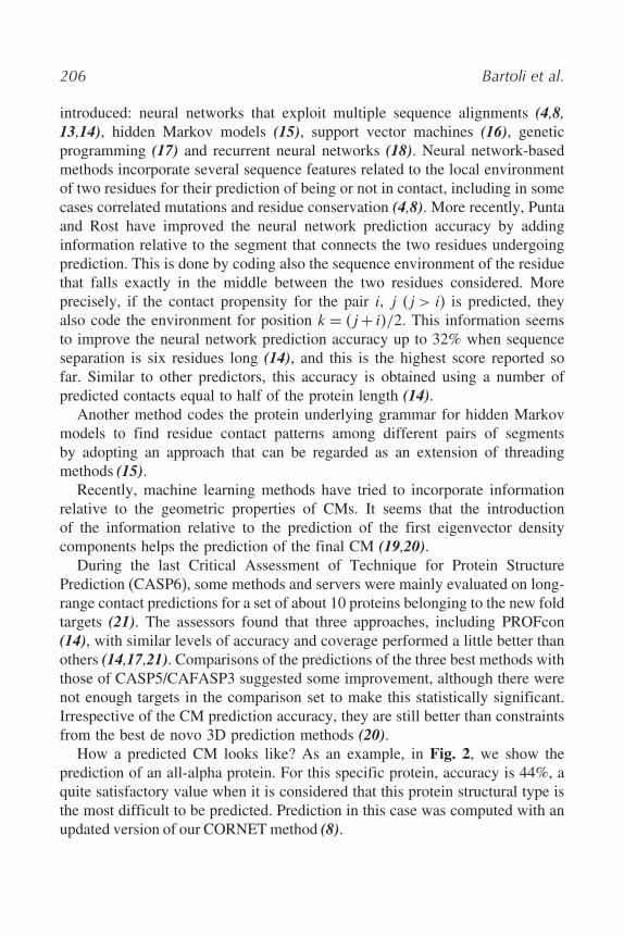
How a predicted CM looks like? As an example, in Fig. 2, we show theprediction of an all-alpha protein. For this specific protein, accuracy is 44%, aquite satisfactory value when it is considered that this protein structural type isthe most difficult to be predicted. Prediction in this case was computed with anupdated version of our CORNETmethod (8).

Protein Contact Maps 207

Fig. 2. Real versus predicted contact map of the $-subunit of the human Farne-syltransferase (PDB code: 1LD8 chain A). On the left side of the plot the black dotsindicate the predicted L/2 contact residues. On the right side, in grey, the real residuecontacts are shown (cut-off radius is 8.0Å centered at the CB atoms and sequenceseparation !6). In the corner on the right, the protein structure is shown, highlightedin black, the correctly predicted contacts. On this protein, our neural network-basedpredictor reaches an accuracy equal to 44%.

5. Small World and Contact MapsUnfortunately we use CMs, we predict them, but we are still unhappy. How

do we improve our methods and our prediction? The solution is still to be found.In the meantime, we suggest another perspective in the following sections.

208 Bartoli et al.

5.1. Small World

To overview some recent literature on proteins, we should introduce a fewconcepts explaining what ‘small world’ is and how it has been used to highlightprotein folding properties.

In the mid-1990s, Duncan Watts, while studying for his PhD in AppliedMathematics, was invited to study a very particular problem: how cricketssynchronize their singing (22). He was convinced that, to deeply understandthis problem, he had to observe the way the crickets pay attention to eachother. This is the starting point of the study of networks under a differentperspective than that of random networks that were previously introduced byErdós and Rényi ((22) and references therein). Watts started his study on socialnetworks trying to answer to a simple question: how many probabilities arethere that two persons, both my friends, know each other? With his ProfessorSteven Strogatz, he found that social networks were clustered and not randomlydistributed and that the same paradigm could model dynamical relations inmany different systems (22).

To explain the omnipresence of clustering in real world networks, Wattsand Strogatz (23) proposed a new connection topology called a ‘small world’network, showing that it can be interpolated between regular and randomnetworks with a random rewiring procedure. According to this model, smallworld systems can be highly clustered, like regular graphs, and at the same timethey are endowed with a small average path length, as it is for random networks.

Watts and Strogatz (23) introduced two numbers to describe the charac-teristics of small world networks: the characteristic path length L and theclustering coefficient C. L is given by the number of edges in the shortest pathbetween two vertices, averaged over all pairs of vertices:

L= 2N &N #1'

N#1!

i=1

N!

j=i+1

Lij"

where Lij is the shortest path length between vertices i and j.Supposing that a vertex k has Nk neighbours, then at the most Nk&Nk#1'/2

edges can exist between them. If nk is the actual number of edges among theneighbours, then C is defined as:

C = 1N

N!

k=1

nk

Nk &Nk#1'/2(

L measures the typical separation between two vertices in the graph (a globalproperty) and C is a measure of local clustering or cliquishness of a typicalneighbourhood (a local property) (23).

Protein Contact Maps 209

5.2. Small World and Protein Structures

The extension of the small world view to proteins was straightforward.Vendruscolo et al. (24) showed that protein structures have small worldtopology. The small world behaviour of protein structures is reflected by thepresence in their graph of a relatively small number of vertices with manyconnections (24). Two residues are considered as connected if the distancebetween their CA atoms is less than a threshold distance fixed at 8.5Å. Byanalysing a data set of 978 representative proteins, it was found that theaverage value of L is 4(1±0(9 and that of C is 0(58±0(04. These values werecompared with those obtained for random and regular graphs. By assumingthat K is the average number of links in the graph (the average number ofcontacts in a protein) and N is the number of vertices (protein residues), thenLrandom & lnN/ lnK and Crandom & K/N ; Lregular & N &N +K#2'/2K &N #1'and Cregular & 3 &K#2'/4 &K#1' (25). Values of 2(4±0(3 and 0(08±0(06 werereported for Lrandom and Crandom respectively; Lregular and Cregular were 10(4±7(0and 0(67±0(04, respectively (24).

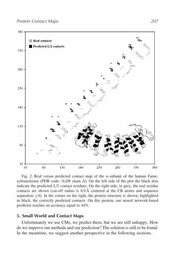
In this chapter for sake of clarity and with the specific aim of relating thesmall world representation to CMs (see below), we perform the same type ofanalysis on a new and a more selected data set of non-redundant mono-domainproteins (497 proteins) (see Fig. 3). We reached similar conclusions as before(24), obtaining L and C equal to 3(9± 0(9 and 0(57± 0(03, respectively. Forour data set, Lrandom is 2(1± 0(2, Crandom is 0(08± 0(04, Lregular is 8(7± 4(2and Cregular is 0(67±0(01, confirming again that Lrandom < L < Lregular and thatCrandom < C< Cregular, a key conclusion for resorting small world behaviour.

Small world view was adopted also for homopolymers obtained with a CMdynamics (26) and for atomic clusters obtained with Lennard–Jones interactionswith a Monte Carlo method (27). In both cases, the values of C and L werefound similar to those of proteins, indicating a small world topology also forthese systems. It was therefore concluded that protein chain connectivity playsa minor role in the small world behaviour and that for a globular protein thesmall world character would mainly arise from the overall geometry (surfaceto volume ratio) (24).

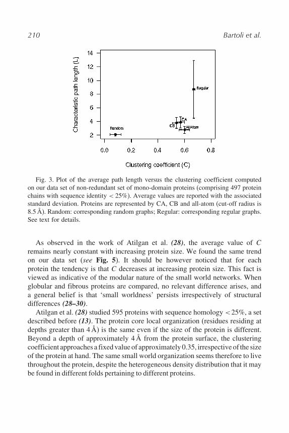
What we did in house was substantially to add to these concepts by analysingother properties of our non-redundant protein set that have been related to smallworld behaviour. Another tendency that shows this property is that L increaseslinearly with log N (as a measure of the protein length) and that the slope ishigher than the random reference case (see Fig. 4). This type of plot is frequentin the pertinent literature (28,29). In our case, we add to the conclusion byanalysing a non-redundant set of mono-domain proteins.

210 Bartoli et al.

Fig. 3. Plot of the average path length versus the clustering coefficient computedon our data set of non-redundant set of mono-domain proteins (comprising 497 proteinchains with sequence identity < 25%). Average values are reported with the associatedstandard deviation. Proteins are represented by CA, CB and all-atom (cut-off radius is8.5Å). Random: corresponding random graphs; Regular: corresponding regular graphs.See text for details.

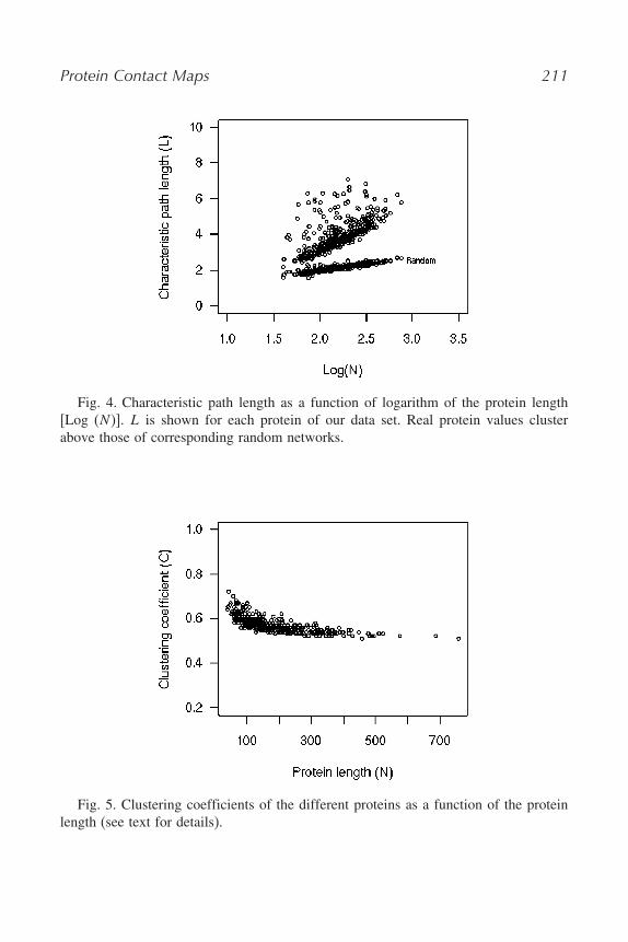
As observed in the work of Atilgan et al. (28), the average value of Cremains nearly constant with increasing protein size. We found the same trendon our data set (see Fig. 5). It should be however noticed that for eachprotein the tendency is that C decreases at increasing protein size. This fact isviewed as indicative of the modular nature of the small world networks. Whenglobular and fibrous proteins are compared, no relevant difference arises, anda general belief is that ‘small worldness’ persists irrespectively of structuraldifferences (28–30).

Atilgan et al. (28) studied 595 proteins with sequence homology<25%, a setdescribed before (13). The protein core local organization (residues residing atdepths greater than 4Å) is the same even if the size of the protein is different.Beyond a depth of approximately 4Å from the protein surface, the clusteringcoefficient approaches a fixedvalueof approximately 0.35, irrespective of the sizeof the protein at hand. The same small world organization seems therefore to livethroughout the protein, despite the heterogeneous density distribution that it maybe found in different folds pertaining to different proteins.

Protein Contact Maps 211

Fig. 4. Characteristic path length as a function of logarithm of the protein length[Log (N )]. L is shown for each protein of our data set. Real protein values clusterabove those of corresponding random networks.

Fig. 5. Clustering coefficients of the different proteins as a function of the proteinlength (see text for details).

212 Bartoli et al.

5.3. Local Versus Global Contacts

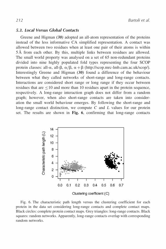
Greene and Higman (30) adopted an all-atom representation of the proteinsinstead of the less informative CA simplified representation. A contact wasallowed between two residues when at least one pair of their atoms is within5Å from each other. By this, multiple links between residues are allowed.The small world property was analysed on a set of 65 non-redundant proteinsdivided into nine highly populated fold types representing the four SCOPprotein classes: all-$, all-%, $/%, $+% (http://scop.mrc-lmb.cam.ac.uk/scop/).Interestingly Greene and Higman (30) found a difference of the behaviourbetween what they called networks of short-range and long-range contacts.Interactions are considered short range or long range if they occur betweenresidues that are $10 and more than 10 residues apart in the protein sequence,respectively. A long-range interaction graph does not differ from a randomgraph; however, when also short-range contacts are taken into consider-ation the small world behaviour emerges. By following the short-range andlong-range contact distinction, we compute C and L values for our proteinset. The results are shown in Fig. 6, confirming that long-range contacts

Fig. 6. The characteristic path length versus the clustering coefficient for eachprotein in the data set considering long-range contacts and complete contact maps.Black circles: complete protein contact maps. Grey triangles: long-range contacts. Blacksquares: random networks. Apparently, long-range contacts overlap with correspondingrandom networks.

Protein Contact Maps 213

can be modelled by a random graph and that small world properties emergeonly when the whole CM is considered.

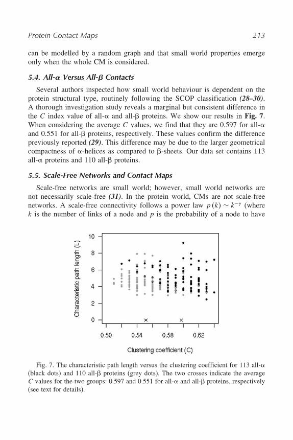
5.4. All-! Versus All-" Contacts

Several authors inspected how small world behaviour is dependent on theprotein structural type, routinely following the SCOP classification (28–30).A thorough investigation study reveals a marginal but consistent difference inthe C index value of all-$ and all-% proteins. We show our results in Fig. 7.When considering the average C values, we find that they are 0.597 for all-$and 0.551 for all-% proteins, respectively. These values confirm the differencepreviously reported (29). This difference may be due to the larger geometricalcompactness of $-helices as compared to %-sheets. Our data set contains 113all-$ proteins and 110 all-% proteins.

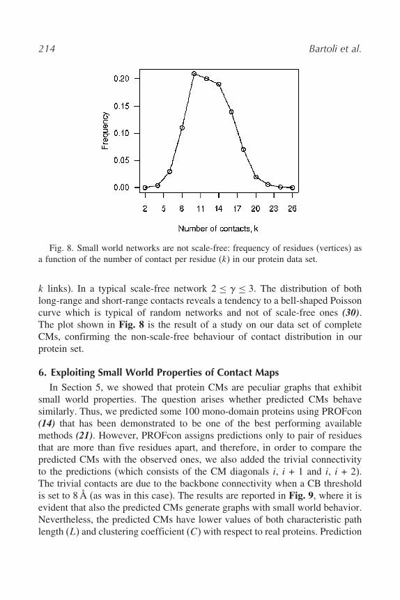
5.5. Scale-Free Networks and Contact Maps

Scale-free networks are small world; however, small world networks arenot necessarily scale-free (31). In the protein world, CMs are not scale-freenetworks. A scale-free connectivity follows a power law p &k' & k#) (wherek is the number of links of a node and p is the probability of a node to have

Fig. 7. The characteristic path length versus the clustering coefficient for 113 all-$(black dots) and 110 all-% proteins (grey dots). The two crosses indicate the averageC values for the two groups: 0.597 and 0.551 for all-$ and all-% proteins, respectively(see text for details).

214 Bartoli et al.

Fig. 8. Small world networks are not scale-free: frequency of residues (vertices) asa function of the number of contact per residue (k) in our protein data set.

k links). In a typical scale-free network 2 $ ) $ 3. The distribution of bothlong-range and short-range contacts reveals a tendency to a bell-shaped Poissoncurve which is typical of random networks and not of scale-free ones (30).The plot shown in Fig. 8 is the result of a study on our data set of completeCMs, confirming the non-scale-free behaviour of contact distribution in ourprotein set.

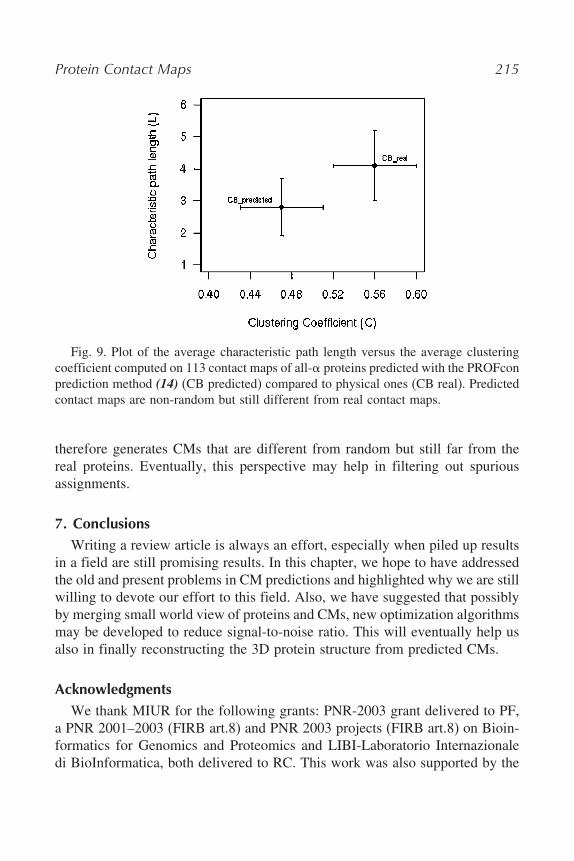
6. Exploiting Small World Properties of Contact MapsIn Section 5, we showed that protein CMs are peculiar graphs that exhibit

small world properties. The question arises whether predicted CMs behavesimilarly. Thus, we predicted some 100 mono-domain proteins using PROFcon(14) that has been demonstrated to be one of the best performing availablemethods (21). However, PROFcon assigns predictions only to pair of residuesthat are more than five residues apart, and therefore, in order to compare thepredicted CMs with the observed ones, we also added the trivial connectivityto the predictions (which consists of the CM diagonals i, i + 1 and i, i + 2).The trivial contacts are due to the backbone connectivity when a CB thresholdis set to 8Å (as was in this case). The results are reported in Fig. 9, where it isevident that also the predicted CMs generate graphs with small world behavior.Nevertheless, the predicted CMs have lower values of both characteristic pathlength (L) and clustering coefficient (C) with respect to real proteins. Prediction

Protein Contact Maps 215

Fig. 9. Plot of the average characteristic path length versus the average clusteringcoefficient computed on 113 contact maps of all-$ proteins predicted with the PROFconprediction method (14) (CB predicted) compared to physical ones (CB real). Predictedcontact maps are non-random but still different from real contact maps.

therefore generates CMs that are different from random but still far from thereal proteins. Eventually, this perspective may help in filtering out spuriousassignments.

7. ConclusionsWriting a review article is always an effort, especially when piled up results

in a field are still promising results. In this chapter, we hope to have addressedthe old and present problems in CM predictions and highlighted why we are stillwilling to devote our effort to this field. Also, we have suggested that possiblyby merging small world view of proteins and CMs, new optimization algorithmsmay be developed to reduce signal-to-noise ratio. This will eventually help usalso in finally reconstructing the 3D protein structure from predicted CMs.

AcknowledgmentsWe thank MIUR for the following grants: PNR-2003 grant delivered to PF,

a PNR 2001–2003 (FIRB art.8) and PNR 2003 projects (FIRB art.8) on Bioin-formatics for Genomics and Proteomics and LIBI-Laboratorio Internazionaledi BioInformatica, both delivered to RC. This work was also supported by the

216 Bartoli et al.

Biosapiens Network of Excellence project (a grant of the European Unions VIFramework Programme).

References1. Havel, T. F. (1998). Distance geometry: theory, algorithms, and chemical appli-

cations. Encyclopedia of Computational Chemistry. John Wiley & Sons, NewYork.

2. Vendruscolo, M. and Domany, E. (1999). Protein folding using contact maps.arXiv cond-mat, 9901215.

3. Bohr, J., Bohr, H., Brunak, S., Cotterill, R. M., Fredholm, H., Lautrup, B. andPetersen, S. B. (1993). Protein structures from distance inequalities. Journal ofMolecular Biology 231, 861–869.

4. Fariselli, P., Olmea, O., Valencia, A. and Casadio, R. (2001). Progress in predictinginter-residue contacts of proteins with neural networks and correlated mutations.Proteins Suppl 5, 157–162.

5. Galaktionov, S. G. and Marshall, G. R. (1994). 27th Annual Hawaii InternationalConference on System Sciences (HICSS-27), Maui, Hawaii.

6. Baldi, P. and Brunak S. (2001). Bioinformatics: The Machine Learning Approach,A Bradford Book, Second edition. MIT Press, Cambridge.

7. Goldman, D., Istrail, S. and Papadimitriou, C. (1999). Algorithmic aspects ofprotein structure similarity. Proceedings of the 40th IEEE Symposium on Founda-tions of Computer Science, New York, (USA), 512–522.

8. Fariselli, P., Olmea, O., Valencia, A. and Casadio, R. (2001). Prediction of contactmaps with neural networks and correlated mutations. Protein Engineering 14,835–843.

9. Porto, M., Bastolla, U., Roman, H. E. and Vendruscolo, M. (2004). Reconstructionof protein structures from a vectorial representation. Physical Review Letters 92,218101.

10. Pollastri, G., Baldi, P., Fariselli, P. and Casadio, R. (2002). Prediction of coordi-nation number and relative solvent accessibility in proteins. Proteins 47(2),142–153.

11. Goebel, U., Sander, C., Schneider, R. and Valencia, A. (1994). Correlatedmutations and residue contacts in proteins. Proteins 18, 309–317.

12. Olmea, O. and Valencia, A. (1997). Improving contact predictions by the combi-nation of correlated mutations and other sources of sequence information. Folding& Design 2, S25–S32.

13. Fariselli, P. and Casadio, R. (1999). A neural network based predictor of residuecontacts in proteins. Protein Engineering 12, 15–21.

14. Punta, M. and Rost, B. (2005). PROFcon: novel prediction of long-range contacts.Bioinformatics 21, 2960–2968.

Protein Contact Maps 217

15. Bystroff, C. and Shao, Y. (2002). Fully automated ab initio protein structureprediction using I-SITES, HMMSTR and ROSETTA. Bioinformatics 18 Suppl 1,S54–S61.

16. Zhao, Y. and Karypis, G. (2003). 3rd IEEE International Conference on Bioinfor-matics and Bioengineering (BIBE).

17. MacCallum, R. M. (2004). Striped sheets and protein contact prediction. Bioinfor-matics 20 Suppl 1, I224–I231.

18. Pollastri, G. and Baldi, P. (2002). Prediction of contact maps by GIOHMMs andrecurrent neural networks using lateral propagation from all four cardinal corners.Bioinformatics 18 Suppl 1, S62–S70.

19. Vullo, A., Walsh, I. and Pollastri, G. (2006). A two-stage approach for improvedprediction of residue contact maps. BMC Bioinformatics 7, 180.

20. Eyrich, V. A., Przybylski, D., Koh, I. Y., Grana, O., Pazos, F., Valencia, A. andRost, B. (2003). CAFASP3 in the spotlight of EVA. Proteins 53 Suppl 6, 548–560.

21. Grana, O., Baker, D., MacCallum, R. M., Meiler, J., Punta, M., Rost, B.,Tress, M. L. and Valencia, A. (2005). CASP6 assessment of contact prediction.Proteins 61 Suppl 7, 214–224.

22. Barabasi, A. L. (2003). Linked: The New Science of Networks, Perseus Publishing,Cambridge, Massachusetts.

23. Watts, D. J. and Strogatz, S. H. (1998). Collective dynamics of ’small-world’networks. Nature 393, 440–442.

24. Vendruscolo, M., Dokholyan, N. V., Paci, E. and Karplus, M. (2002). Small-worldview of the amino acids that play a key role in protein folding. Physical Review.E, Statistical, Nonlinear, and Soft Matter Physics 65, 061910.

25. Watts, D. J. (1999). Small Worlds. The Dynamics of Networks Between Order andRandomness, Princeton University Press, Princeton, New Jersey.

26. Vendruscolo, M. and Domany, E. (1998). Efficient dynamics in the space ofcontact maps. Folding & Design 3, 329–336.

27. Andricioaei, I., Voter, A. F. and Straub, J. E. (2001). Smart Darting Monte Carlo.The Journal of Chemical Physics 114, 6994–7000.

28. Atilgan, A. R., Akan, P. and Baysal, C. (2004). Small-world communication ofresidues and significance for protein dynamics. Biophysical Journal 86, 85–91.

29. Bagler, G. and Sinha, S. (2005). Network properties of protein structures. PhysicaA 346, 27–33.

30. Greene, L. H. and Higman, V. A. (2003). Uncovering network systems withinprotein structures. Journal of Molecular Biology 334, 781–791.

31. Barabasi, A. L. and Albert, R. (1999). Emergence of scaling in random networks.Science 286, 509–512.