to be submitted to ApJ

Preprint typeset using LATEX style emulateapj v. 12/16/11

THE PIPER SURVEY: I. AN INITIAL LOOK AT THE INTRACLUSTER GLOBULARCLUSTER POPULATION IN THE PERSEUS CLUSTER

William E. Harris

Department of Physics & AstronomyMcMaster University

Hamilton ON L8S 4M1, Canada

Patrick R. Durrell

Department of Physics and AstronomyYoungstown State UniversityYoungstown OH 44555, USA

Aaron J. Romanowsky

Department of Physics & Astronomy, San Jose State UniversityOne Washington Square, San Jose CA 95192, USA

John Blakeslee

National Research Council of CanadaHerzberg Astronomy and Astrophysics Research Centre

Victoria BC, Canada

Jean Brodie

University of California Observatories1156 High Street, Santa Cruz CA 95064, USA

Steven Janssens

Department of Astronomy and AstrophysicsUniversity of Toronto, 50 St. George St, Toronto ON M5S 3H4, Canada

Thorsten Lisker

Astronomisches Rechen-Institut, Zentrum fur Astronomie der Universitat Heidelberg, Monchhofstrae 12-14, 69120Heidelberg, Germany

Sakurako Okamoto

Shanghai Astronomical Observatory80 Nandan Road, Shanghai 200030, China

Carolin Wittmann

Astronomisches Rechen-Institut, Zentrum fur Astronomie der Universitat Heidelberg, Monchhofstrae 12-14, 69120Heidelberg, Germany

(Dated: August 21, 2018)to be submitted to ApJ

ABSTRACT

We describe the goals and first results of a Program for Imaging of the PERseuscluster of galaxies (PIPER). The first phase of the program builds on imagingof fields obtained with the Hubble Space Telescope ACS/WFC and WFC3/UVIScameras. Our PIPER target fields with HST in total include major early-typegalaxies including the active central giant NGC 1275; known Ultra-Diffuse Galax-ies; and the Intracluster Medium. The resulting photometry, in B and I, reachesdeep enough to resolve and measure the globular cluster (GC) populations in thePerseus member galaxies. Here we present initial results for three pairs of fieldsthat confirm the presence of Intracluster GCs as distant as 740 kpc from the Perseuscenter, or 40% of the virial radius of the cluster. The majority of these IntraclusterGCs are identifiably blue (metal-poor) but there is a trace of a red (metal-rich)

2 Harris et al.

component as well, even at these very remote distances.Keywords: galaxies: formation — galaxies: star clusters — globular clusters: gen-

eral

1. INTRODUCTION

Perseus (Abell 426) at d = 75 Mpc offers arich and fascinating laboratory for galaxy evo-lution, but it has not yet gained the level ofattention that has been given, for example, toVirgo or Coma. Perseus has a velocity dis-persion in the range σv ≃ 1000 − 1300 kms−1, among the highest of clusters in the lo-cal universe (Kent & Sargent 1983; Struble &Rood 1991; Girardi et al. 1996; Weinmann et al.2011); for comparison, the Coma cluster hasσv = 1100 km s−1 (Colless & Dunn 1996). Thetotal mass of Perseus is almost 1015M⊙ (Gi-rardi et al. 1998; Simionescu et al. 2011). En-veloping the cluster is a vast halo of X-ray gasand dark matter with virial radius r200 = 1.8Mpc (Simionescu et al. 2011), comparable tothe most gas-rich and populous galaxy clusters(e.g. Zhao et al. 2013; Loewenstein 1994; Mainet al. 2017).

Like Virgo and Coma, Perseus contains manylarge early-type galaxies, among which themost notable is the central supergiant NGC1275 (= 3C48 = Perseus A), which sits atthe center of the X-ray gas and the dynam-ical center of the cluster. NGC 1275 is per-haps the most extreme case in the local universewhere we see the ongoing growth of a Bright-est Cluster Galaxy (BCG) complete with cool-ing flows, feedback, and extreme star forma-tion rate. Within NGC 1275 is a spectacularweb of Hα filaments extending to more than 30kpc from galaxy center, which itself contains∼ 1011M⊙ of molecular gas and extended re-gions of star formation (e.g. Fabian et al. 2011;Matsushita et al. 2013; Canning et al. 2014).

In this paper, we describe a Program forImaging of PERseus (called PIPER) currentlyunderway that is intended to attack four differ-ent program goals through the use of globularcluster (GC) populations.

(1) In recent years it has become clear that richclusters of galaxies are hosts for large numbersof Ultra-Diffuse Galaxies (UDGs), currentlya focus of considerable interest (van Dokkumet al. 2015a,b; Koda et al. 2015; Martınez-Delgado et al. 2016; Roman & Trujillo 2017;Papastergis et al. 2017; Amorisco et al. 2018).Perseus is already known to hold many UDGcandidates (Wittmann et al. 2017), giving usthe chance to improve our understanding oftheir demographics. Some UDGs in turn seemto have remarkably populous systems of GCs

harris@physics.mcmaster.ca

relative to their low luminosities (Peng & Lim2016; Beasley & Trujillo 2016; van Dokkumet al. 2016, 2018), indicating that they havemassive dark halos and extremely high mass-to-light ratios (Harris et al. 2017b), while othersare quite GC-poor (Lim et al. 2018; Amoriscoet al. 2018). No highly consistent pattern hasyet emerged, and at least some of these extremegalaxies may violate the near-constant ratio ofGC system mass to halo (virial) mass obeyedby more luminous galaxies (Hudson et al. 2014;Durrell et al. 2014; Harris et al. 2017b) or sim-ply show considerable scatter around that rela-tion (Toloba et al. 2018; El-Badry et al. 2018;Amorisco et al. 2018).

(2) As a rich and dynamically active cluster,Perseus should also have stellar Intra-ClusterLight (ICL) built from disrupted or strippedmember galaxies (e.g. Burke et al. 2012; Ramoset al. 2015; Ramos-Almendares et al. 2018).In such clusters the ICL can make up typi-cally 10–30% of the total stellar mass. Becausethe ICL is actively growing particularly sincez = 1, the sheer amount of ICL and its degreeof substructure (clumpiness and tidal streams)probe the dynamical state of the entire clus-ter. But the stellar ICL is extremely diffuse anddifficult to map out with conventional surface-brightness photometry over a field as wide asthe ∼ 1◦ diameter of Perseus. For such alow signal, a more effective tracer is one forwhich the background ‘noise’ can be reducedto near-zero levels. As will be shown below,GCs fit this bill beautifully: they are individ-ually luminous, easy to isolate, and can bereached by HST for galaxies out to ∼ 250Mpc or more (Harris et al. 2016). A pre-liminary investigation of the GC populationsin MAST Archival fields within Perseus hasshown that an Intra-Cluster Globular Clus-ter (ICGC) population exists (Harris & Mul-holland 2017, hereafter referred to as HM17)though the sheer amount of it is still quite un-certain. Substantial ICGC numbers have beendetected in other large clusters including Virgo(Durrell et al. 2014), Coma (Peng et al. 2011),A1185 (West et al. 2011), and A1689 (Alamo-Martınez & Blakeslee 2017). Perhaps mostimportantly, multiband photometry also auto-matically yields their metallicity distributionfunction (MDF) since GC color is a monotonicfunction of [Fe/H] and is quite insensitive to age(e.g. Peng et al. 2006). The extremely faint,diffuse, integrated stellar light cannot providethis level of insight.

3

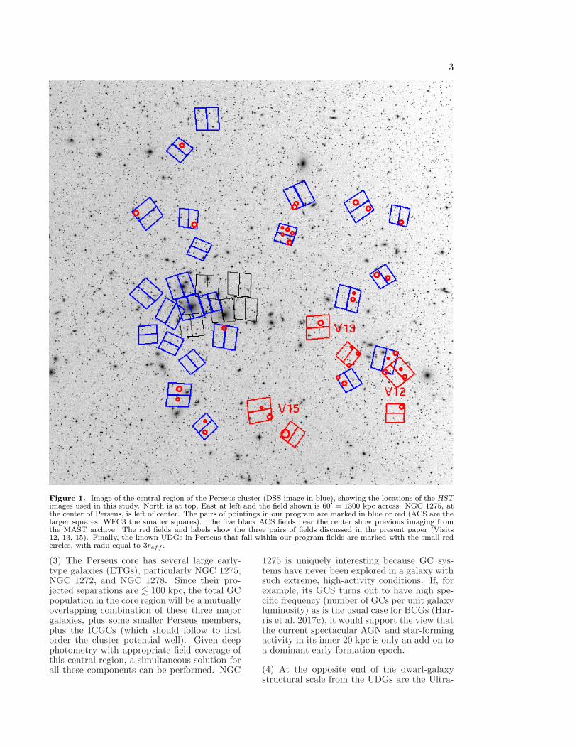
Figure 1. Image of the central region of the Perseus cluster (DSS image in blue), showing the locations of the HST

images used in this study. North is at top, East at left and the field shown is 60′ = 1300 kpc across. NGC 1275, atthe center of Perseus, is left of center. The pairs of pointings in our program are marked in blue or red (ACS are thelarger squares, WFC3 the smaller squares). The five black ACS fields near the center show previous imaging fromthe MAST archive. The red fields and labels show the three pairs of fields discussed in the present paper (Visits12, 13, 15). Finally, the known UDGs in Perseus that fall within our program fields are marked with the small redcircles, with radii equal to 3reff .

(3) The Perseus core has several large early-type galaxies (ETGs), particularly NGC 1275,NGC 1272, and NGC 1278. Since their pro-jected separations are . 100 kpc, the total GCpopulation in the core region will be a mutuallyoverlapping combination of these three majorgalaxies, plus some smaller Perseus members,plus the ICGCs (which should follow to firstorder the cluster potential well). Given deepphotometry with appropriate field coverage ofthis central region, a simultaneous solution forall these components can be performed. NGC

1275 is uniquely interesting because GC sys-tems have never been explored in a galaxy withsuch extreme, high-activity conditions. If, forexample, its GCS turns out to have high spe-cific frequency (number of GCs per unit galaxyluminosity) as is the usual case for BCGs (Har-ris et al. 2017c), it would support the view thatthe current spectacular AGN and star-formingactivity in its inner 20 kpc is only an add-on toa dominant early formation epoch.

(4) At the opposite end of the dwarf-galaxystructural scale from the UDGs are the Ultra-

4 Harris et al.

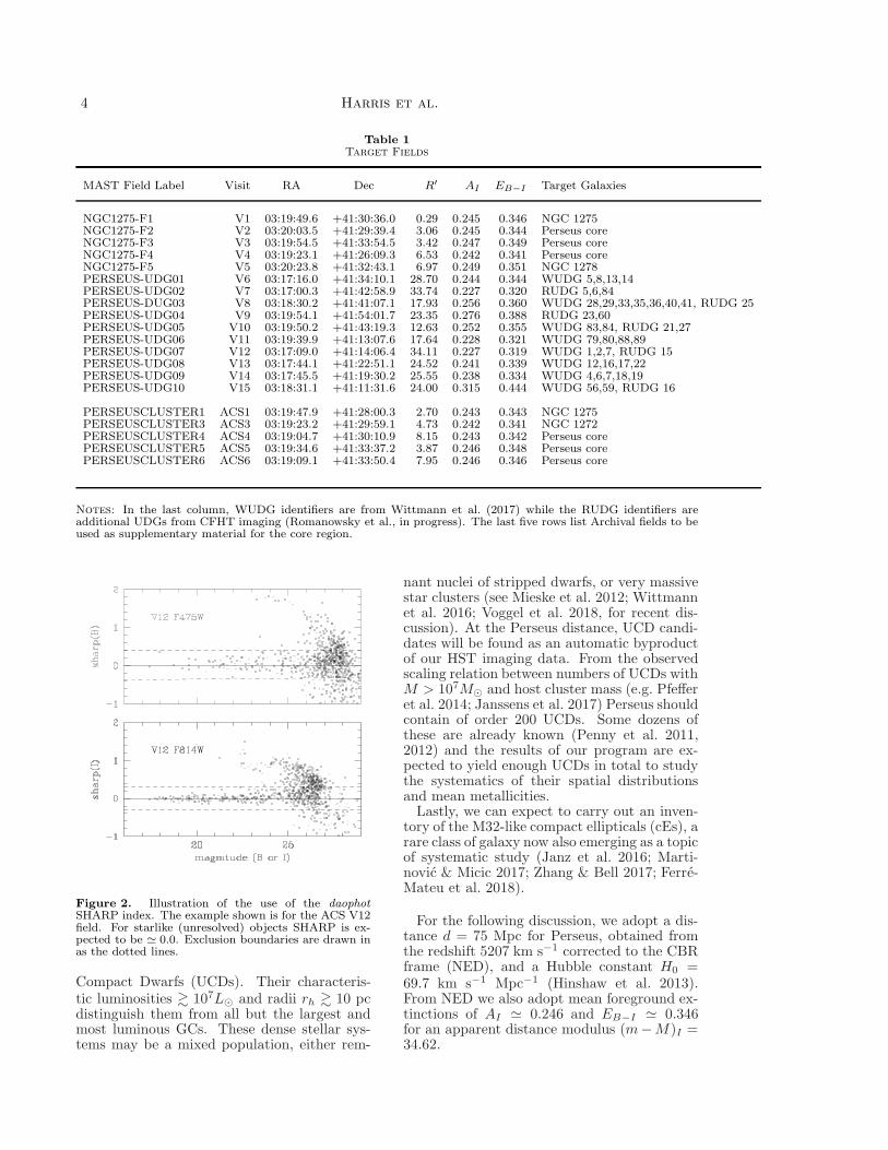
Table 1Target Fields

MAST Field Label Visit RA Dec R′ AI EB−I Target Galaxies

NGC1275-F1 V1 03:19:49.6 +41:30:36.0 0.29 0.245 0.346 NGC 1275NGC1275-F2 V2 03:20:03.5 +41:29:39.4 3.06 0.245 0.344 Perseus coreNGC1275-F3 V3 03:19:54.5 +41:33:54.5 3.42 0.247 0.349 Perseus coreNGC1275-F4 V4 03:19:23.1 +41:26:09.3 6.53 0.242 0.341 Perseus coreNGC1275-F5 V5 03:20:23.8 +41:32:43.1 6.97 0.249 0.351 NGC 1278PERSEUS-UDG01 V6 03:17:16.0 +41:34:10.1 28.70 0.244 0.344 WUDG 5,8,13,14PERSEUS-UDG02 V7 03:17:00.3 +41:42:58.9 33.74 0.227 0.320 RUDG 5,6,84PERSEUS-DUG03 V8 03:18:30.2 +41:41:07.1 17.93 0.256 0.360 WUDG 28,29,33,35,36,40,41, RUDG 25PERSEUS-UDG04 V9 03:19:54.1 +41:54:01.7 23.35 0.276 0.388 RUDG 23,60PERSEUS-UDG05 V10 03:19:50.2 +41:43:19.3 12.63 0.252 0.355 WUDG 83,84, RUDG 21,27PERSEUS-UDG06 V11 03:19:39.9 +41:13:07.6 17.64 0.228 0.321 WUDG 79,80,88,89PERSEUS-UDG07 V12 03:17:09.0 +41:14:06.4 34.11 0.227 0.319 WUDG 1,2,7, RUDG 15PERSEUS-UDG08 V13 03:17:44.1 +41:22:51.1 24.52 0.241 0.339 WUDG 12,16,17,22PERSEUS-UDG09 V14 03:17:45.5 +41:19:30.2 25.55 0.238 0.334 WUDG 4,6,7,18,19PERSEUS-UDG10 V15 03:18:31.1 +41:11:31.6 24.00 0.315 0.444 WUDG 56,59, RUDG 16

PERSEUSCLUSTER1 ACS1 03:19:47.9 +41:28:00.3 2.70 0.243 0.343 NGC 1275PERSEUSCLUSTER3 ACS3 03:19:23.2 +41:29:59.1 4.73 0.242 0.341 NGC 1272PERSEUSCLUSTER4 ACS4 03:19:04.7 +41:30:10.9 8.15 0.243 0.342 Perseus corePERSEUSCLUSTER5 ACS5 03:19:34.6 +41:33:37.2 3.87 0.246 0.348 Perseus corePERSEUSCLUSTER6 ACS6 03:19:09.1 +41:33:50.4 7.95 0.246 0.346 Perseus core

Notes: In the last column, WUDG identifiers are from Wittmann et al. (2017) while the RUDG identifiers areadditional UDGs from CFHT imaging (Romanowsky et al., in progress). The last five rows list Archival fields to beused as supplementary material for the core region.

Figure 2. Illustration of the use of the daophotSHARP index. The example shown is for the ACS V12field. For starlike (unresolved) objects SHARP is ex-pected to be ≃ 0.0. Exclusion boundaries are drawn inas the dotted lines.

Compact Dwarfs (UCDs). Their characteris-tic luminosities & 107L⊙ and radii rh & 10 pcdistinguish them from all but the largest andmost luminous GCs. These dense stellar sys-tems may be a mixed population, either rem-

nant nuclei of stripped dwarfs, or very massivestar clusters (see Mieske et al. 2012; Wittmannet al. 2016; Voggel et al. 2018, for recent dis-cussion). At the Perseus distance, UCD candi-dates will be found as an automatic byproductof our HST imaging data. From the observedscaling relation between numbers of UCDs withM > 107M⊙ and host cluster mass (e.g. Pfefferet al. 2014; Janssens et al. 2017) Perseus shouldcontain of order 200 UCDs. Some dozens ofthese are already known (Penny et al. 2011,2012) and the results of our program are ex-pected to yield enough UCDs in total to studythe systematics of their spatial distributionsand mean metallicities.

Lastly, we can expect to carry out an inven-tory of the M32-like compact ellipticals (cEs), arare class of galaxy now also emerging as a topicof systematic study (Janz et al. 2016; Marti-novic & Micic 2017; Zhang & Bell 2017; Ferre-Mateu et al. 2018).

For the following discussion, we adopt a dis-tance d = 75 Mpc for Perseus, obtained fromthe redshift 5207 km s−1 corrected to the CBRframe (NED), and a Hubble constant H0 =69.7 km s−1 Mpc−1 (Hinshaw et al. 2013).From NED we also adopt mean foreground ex-tinctions of AI ≃ 0.246 and EB−I ≃ 0.346for an apparent distance modulus (m−M)I =34.62.

5

The outline of this paper is as follows: Sec-tion 2 describes the characteristics of our imag-ing database and the photometric measurementtechniques directed towards isolating the GCcandidates. Section 3 presents in turn thecolor-magnitude distribution of the GCs in eachtarget field, their effective radii, their luminos-ity distribution, and their color distribution.Section 4 concludes with a brief summary.

2. DATABASE AND OBSERVATIONALSTRATEGY

Our new HST imaging data for PIPER isfrom Cycle 25 program 15235 (PI Harris). TheACS/WFC and WFC3/UVIS cameras are usedin parallel to obtain exposures of 15 pairs offields scattered across the cluster; these point-ings are shown in Figure 1 and listed in Ta-ble 1. In the Table, successive columns list theMAST Archive field identifier; the Visit num-ber; the field coordinates (J2000) for the Pri-mary camera pointing in each pair; their pro-jected distance R in arcminutes from NGC 1275(the Perseus center); foreground extinction AI

and reddening EB−I calculated from NED; andthe galaxies included in each pointing.

In Table 1, for Visits 1-5, the ACS camera isthe Primary and WFC3 the Parallel, while forVisits 6-15, WFC3 is the Primary and ACS theParallel.

The core of Perseus, at center-left in the fig-ure, is covered nearly completely out to R ≃

5′ (100 kpc) when supplemented by the ad-ditional five MAST Archive ACS/WFC fieldsalso shown in the figure. The pointings tar-getting the UDGs are in most cases far awayfrom any of the major Perseus galaxies. Thefinal five rows of Table 1 give the locations ofArchival ACS fields from program 10201 (PIConselice) that will also be used to fill in ourcoverage of the Perseus core regions (see alsoHM17). As can be seen in Table 1, the field-to-field differences in foreground reddening aremodest (typically ∆(B − I) . 0.03 mag) withthe exception of the more heavily reddenedV15.

The fields will be referred to below by theirspacecraft Visit number V1–V15. The first fiveVisits are the ones covering the Perseus core,while the remaining 10 are the outer fields se-lected to cover the UDGs. Spacecraft orien-tations were chosen to maximize the numbersof UDGs we could capture. These 10 outlyingfields will also be used to reveal ICGCs, UCDs,and any other types of dwarf-galaxy members.

The schedule of spacecraft visits is spread outover nearly a two-year period from 2017 Oct to2019 March. At time of writing, the first threeimage pairs have been obtained, for V12, V13,and V15. These target three of the most re-mote locations from cluster center. At a scale

of 22 kpc/arcmin for a Perseus distance of 75Mpc, V12 (for example) lies at a projected dis-tance of 740 kpc from Perseus center (cf. Table1), equivalent to 40% of the Perseus virial ra-dius (Simionescu et al. 2011). In the presentpaper, we use the data from these three imagepairs to define a consistent set of measurementprocedures, and to gain an initial look at thefeatures of the ICGC population.

For most of our program goals we need todetect and characterize GCs within Perseus,either in the target galaxies or distributedthroughout the diffuse ICM. Typical GCs havehalf-light diameters 2rh ≃ 5 pc (Harris 1996,2010 edition), which at d = 75 Mpc translatesto 0.014′′, almost an order of magnitude smallerthan the natural 0.1′′ resolution of HST. Thismeans that most GCs belonging to the Perseusgalaxies will be near-starlike (that is, unre-solved) objects, which is a major advantagefor carrying out photometry and for isolatingthem from the field contaminants that are dom-inated by faint, small background galaxies (seebelow). In addition, GCs fall in a relativelynarrow range of color index, permitting fur-ther rejection of very blue or very red contami-nants. This combination of object morphologyand color gives us a very effective filtering pro-cedure to isolate the GC population with a lowlevel of residual contamination.

In all cases our program employs exposuresin filters that maximize signal-to-noise but canalso be transformed to standard (B, I) foreasy comparison with previous GC data in theliterature. The adopted filters are (F475W,F814W) for ACS/WFC; and (F475X, F814W)for WFC3/UVIS. Though WFC3 F475X hasrarely been used, it is significantly broader thanF475W and still transforms well to standard B.For Visits V6-V15, the Primary field is WFC3with total exposure times of 2533 sec in F475Xand 2653 sec in F814W. Four dithered sub-exposures are taken in each case to give a finalimage effectively free of cosmic rays and otherartifacts. The Parallel field is ACS with totalt = 2424 sec (F475W) and 2271 sec (F814W).In what follows, we will refer to the exposurepairs as the B and I images.

The procedure for detection and photometryof the GC candidates is similar to the steps out-lined in, e.g., Harris (2009); Harris et al. (2016)or HM17. We start with the CTE-corrected,drizzled *.drc images provided by MAST. First,both B and I exposures are registered and com-bined to create a master image. Source Extrac-tor (SE) (Bertin & Arnouts 1996) is used tomeasure this master image and to construct afinding list, keeping only objects within the SEparameter range 1.0 . r1/2 . 1.5 px (cf. Harris2009). This first culling step eliminates obvi-

6 Harris et al.

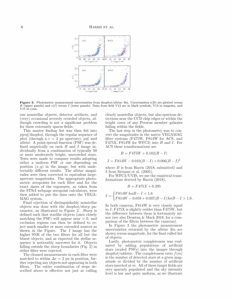
Figure 3. Photometric measurement uncertainties from daophot/allstar fits. Uncertainties e(B) are plotted versusB (upper panels) and e(I) versus I (lower panels). Data from field V12 are in black symbols, V13 in magenta, andV15 in cyan.

ous nonstellar objects, detector artifacts, and(very) occasional severely crowded objects, al-though crowding is not a significant problemfor these extremely sparse fields.

This master finding list was then fed intopyraf/daophot, through the regular sequence ofphot (through a r = 2 px aperture), psf, andallstar. A point-spread function (PSF) was de-fined empirically on each B and I image in-dividually from a combination of typically 50or more moderately bright, uncrowded stars.Tests were made to compare results adoptingeither a uniform PSF or one depending onposition (x, y) in the image, but with unde-tectably different results. The allstar magni-tudes were then corrected to equivalent large-aperture magnitudes. The appropriate photo-metric zeropoints for each filter and for theexact dates of the exposures, as taken fromthe STScI webpage zeropoint calculators, werethen added to put the data onto the VEGA-MAG system.

Final rejection of distinguishably nonstellarobjects was done with the daophot/sharp pa-rameter, as illustrated in Figure 2. Sharp isdefined such that starlike objects (ones closelymatching the PSF) will appear near ≃ 0, andexclusion regions can then be defined to re-ject much smaller or more extended sources asshown in the Figure. The I image has thehigher SNR of the two filters for all but thebluest objects, and as expected the stellar se-quence is noticeably narrower for it. Objectsfalling outside the sharp boundaries (Fig. 2) ineither filter were rejected.

The cleaned measurements in each filter werematched to within ∆r = 2 px in position, fur-ther rejecting any objects not appearing in bothfilters. The entire combination of steps de-scribed above is effective not just at culling

clearly nonstellar objects, but also spurious de-tections near the CCD chip edges or within thebright cores of any Perseus member galaxiesfalling within the fields.

The last step in the photometry was to con-vert the magnitudes in the native VEGAMAGfilter systems (F475W, F814W for ACS, andF475X, F814W for WFC3) into B and I. ForACS these transformations are

B = F475W + 0.182(B − I)

I = F814W − 0.010(B − I) + 0.006(B − I)2

where B is from Harris (2018, submitted) andI from Sirianni et al. (2005).

For WFC3/UVIS, we use the empirical trans-formations derived by Harris (2018),

B = F475X + 0.295

I =

{

F814W forB − I < 1.6

F814W − 0.059 + 0.037(B − I) forB − I > 1.6 .

In both cameras, F814W is very closely equalto I; F475X is slightly redder than F475W, butthe difference between them is fortunately mi-nor (see also Deustua & Mack 2018, for a com-parison of the filters between the cameras).

In Figure 3 the photometric measurementuncertainties returned by the allstar fits areshown versus magnitude, for the final culled listof objects.

Lastly, photometric completeness was eval-uated by adding populations of artificialstars (scaled PSFs) into the images throughdaophot/addstar. The completeness ratio f(m)is the number of detected stars at a given mag-nitude m divided by the number of artificialstars inserted at m. All of these target fields arevery sparsely populated and the sky intensitylevel is low and quite uniform, as we illustrate

7

1 23 44 66 87 109 131 152 174 195 217

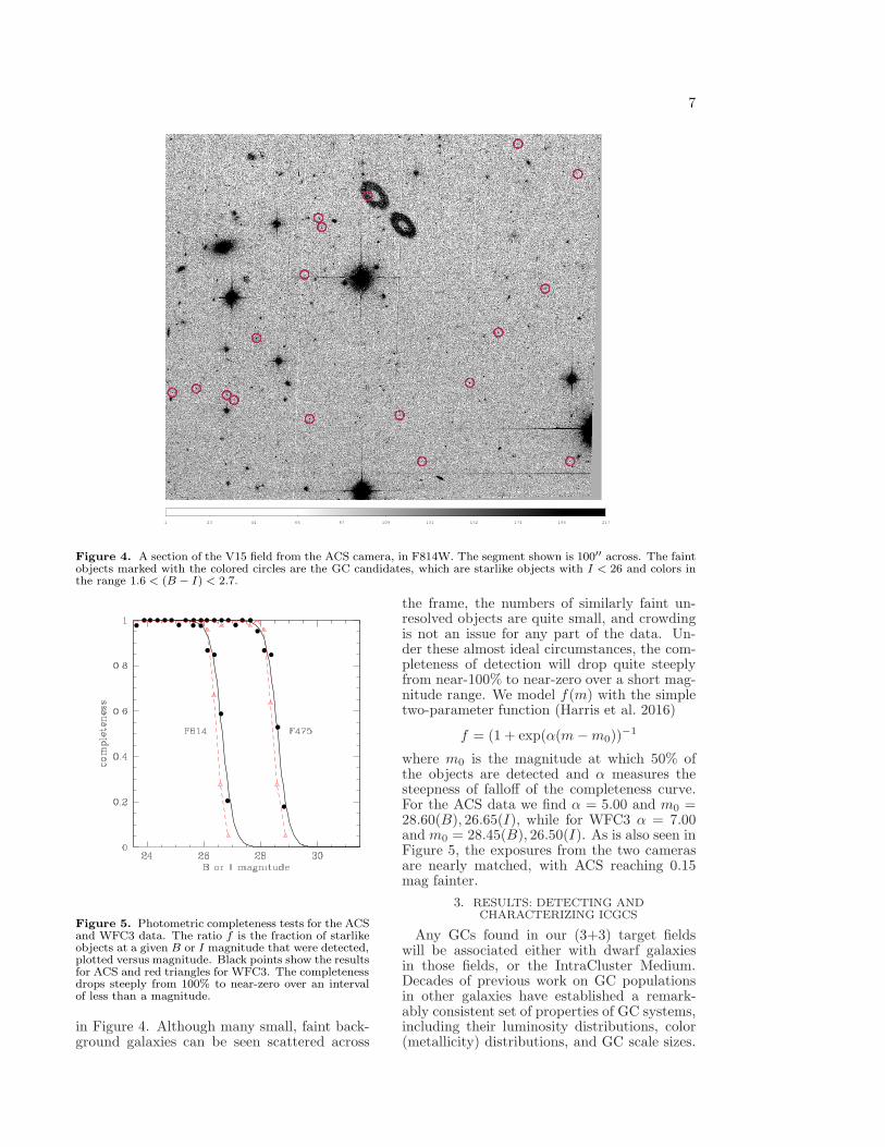
Figure 4. A section of the V15 field from the ACS camera, in F814W. The segment shown is 100′′ across. The faintobjects marked with the colored circles are the GC candidates, which are starlike objects with I < 26 and colors inthe range 1.6 < (B − I) < 2.7.

Figure 5. Photometric completeness tests for the ACSand WFC3 data. The ratio f is the fraction of starlikeobjects at a given B or I magnitude that were detected,plotted versus magnitude. Black points show the resultsfor ACS and red triangles for WFC3. The completenessdrops steeply from 100% to near-zero over an intervalof less than a magnitude.

in Figure 4. Although many small, faint back-ground galaxies can be seen scattered across

the frame, the numbers of similarly faint un-resolved objects are quite small, and crowdingis not an issue for any part of the data. Un-der these almost ideal circumstances, the com-pleteness of detection will drop quite steeplyfrom near-100% to near-zero over a short mag-nitude range. We model f(m) with the simpletwo-parameter function (Harris et al. 2016)

f = (1 + exp(α(m −m0))−1

where m0 is the magnitude at which 50% ofthe objects are detected and α measures thesteepness of falloff of the completeness curve.For the ACS data we find α = 5.00 and m0 =28.60(B), 26.65(I), while for WFC3 α = 7.00and m0 = 28.45(B), 26.50(I). As is also seen inFigure 5, the exposures from the two camerasare nearly matched, with ACS reaching 0.15mag fainter.

3. RESULTS: DETECTING ANDCHARACTERIZING ICGCS

Any GCs found in our (3+3) target fieldswill be associated either with dwarf galaxiesin those fields, or the IntraCluster Medium.Decades of previous work on GC populationsin other galaxies have established a remark-ably consistent set of properties of GC systems,including their luminosity distributions, color(metallicity) distributions, and GC scale sizes.

8 Harris et al.

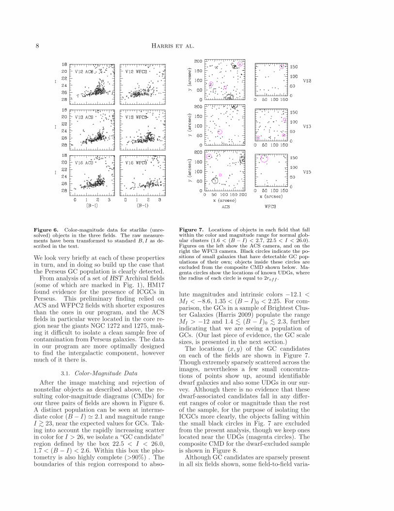
Figure 6. Color-magnitude data for starlike (unre-solved) objects in the three fields. The raw measure-ments have been transformed to standard B, I as de-scribed in the text.

We look very briefly at each of these propertiesin turn, and in doing so build up the case thatthe Perseus GC population is clearly detected.

From analysis of a set of HST Archival fields(some of which are marked in Fig. 1), HM17found evidence for the presence of ICGCs inPerseus. This preliminary finding relied onACS and WFPC2 fields with shorter exposuresthan the ones in our program, and the ACSfields in particular were located in the core re-gion near the giants NGC 1272 and 1275, mak-ing it difficult to isolate a clean sample free ofcontamination from Perseus galaxies. The datain our program are more optimally designedto find the intergalactic component, howevermuch of it there is.

3.1. Color-Magnitude Data

After the image matching and rejection ofnonstellar objects as described above, the re-sulting color-magnitude diagrams (CMDs) forour three pairs of fields are shown in Figure 6.A distinct population can be seen at interme-diate color (B − I) ≃ 2.1 and magnitude rangeI & 23, near the expected values for GCs. Tak-ing into account the rapidly increasing scatterin color for I > 26, we isolate a “GC candidate”region defined by the box 22.5 < I < 26.0,1.7 < (B − I) < 2.6. Within this box the pho-tometry is also highly complete (>90%) . Theboundaries of this region correspond to abso-

Figure 7. Locations of objects in each field that fallwithin the color and magnitude range for normal glob-ular clusters (1.6 < (B − I) < 2.7, 22.5 < I < 26.0).Figures on the left show the ACS camera, and on theright the WFC3 camera. Black circles indicate the po-sitions of small galaxies that have detectable GC pop-ulations of their own; objects inside these circles areexcluded from the composite CMD shown below. Ma-genta circles show the locations of known UDGs, wherethe radius of each circle is equal to 2reff .

lute magnitudes and intrinsic colors −12.1 <MI < −8.6, 1.35 < (B − I)0 < 2.25. For com-parison, the GCs in a sample of Brightest Clus-ter Galaxies (Harris 2009) populate the rangeMI > −12 and 1.4 . (B − I)0 . 2.3, furtherindicating that we are seeing a population ofGCs. (Our last piece of evidence, the GC scalesizes, is presented in the next section.)

The locations (x, y) of the GC candidateson each of the fields are shown in Figure 7.Though extremely sparsely scattered across theimages, nevertheless a few small concentra-tions of points show up, around identifiabledwarf galaxies and also some UDGs in our sur-vey. Although there is no evidence that thesedwarf-associated candidates fall in any differ-ent ranges of color or magnitude than the restof the sample, for the purpose of isolating theICGCs more clearly, the objects falling withinthe small black circles in Fig. 7 are excludedfrom the present analysis, though we keep oneslocated near the UDGs (magenta circles). Thecomposite CMD for the dwarf-excluded sampleis shown in Figure 8.

Although GC candidates are sparsely presentin all six fields shown, some field-to-field varia-

9

tions are noticeable. Even after exclusion of theregions around the obvious dwarfs, the meannumber densities seem clearly larger in some ofthe fields even though all are remote from thePerseus center. If the variations are not duestrictly to simple stochastic differences in analready-low mean density, part of the explana-tion may lie in the particular locations of thesefields: as can be seen in Fig. 1, V12 (ACS)and V13 (both ACS and WFC3) fall along aprominent chain of galaxies running from thePerseus core region (East side) through to IC310 (the giant ETG on the West side, at lowerright in Fig. 1) and beyond. This connectionraises the possibility that ICGCs may also liepreferentially along the same axis. On a scalean order of magnitude larger, the distributionof Perseus galaxies connects with the Perseus-Pisces supercluster (Haynes & Giovanelli 1986;Wegner et al. 1993). By contrast, field V15(ACS and WFC3) lies far off this ridgeline andthere are fewer GCs. In addition, the V12 ACSfield in particular falls near the giant IC 310 (ata mean separation of 90 kpc). The outskirts ofthe IC 310 halo may then also be contributingto the counts in V12/ACS. We will defer fur-ther discussion of these interesting possibilitiesuntil the data are in hand from our completeset of program fields.

3.2. Background Contamination

The fraction of this GC candidate samplethat consists of actual Perseus GCs depends onthe residual level of field contamination in thephotometry – foreground stars and very faint,small background galaxies that managed topass through the culling steps described above.Ideally we would like to assess the contami-nation level from a background control fieldnear but outside Perseus. However, we havefound no suitable material in the MAST archivewith ACS or WFC3 filters in B, I and exposuretimes similar to our data. Instead, as a pre-liminary measure we use data from the HubbleFrontier Fields (Lotz et al. 2017). The Par-allel exposures in the HFF program are withthe ACS/WFC, fall on ‘blank’ fields free of anymajor galaxies or clusters of galaxies, and havelong exposures in F435, F814W that can bereadily transformed to B, I. We have taken ex-posure pairs from the three HFF fields with thelowest Galactic latitudes, and measured themwith exactly the same procedures as for ourPerseus targets. These three HFF fields arelisted in Table 2, giving the Primary targetname, the coordinates of the Parallel fields,their foreground extinction, and the exposuretimes in B and I. (In the Table the exposuretimes are given for the specific image pair se-lected from the much longer list of HFF expo-

sures. In order to match the Perseus data bet-ter, we use these shorter-exposure pairs ratherthan the ultra-deep combined stacks of all ex-posures.) The same quantities are listed forcomparison for our Perseus data.

In Figure 9, the resulting photometry for thethree HFF fields combined (with total area 39arcmin2) is shown after the same process of ob-ject selection and culling of nonstellar objects.Data from each field are corrected to the fore-ground reddening and extinction of Perseus. Intotal, just 19 objects fall clearly within the GC-candidate region defined above, and just 13 inthe range I > 24 where most of the GC candi-dates lie. (Of these 13, there are 0, 8, 5 objectseach from HFF fields 2, 3, 6 respectively. Inthe presence of small-number random varianceit is unclear whether a systematic dependenceon latitude is present.) Since the Perseus fieldsV12,13,15 cover 57.3 arcmin2 in total, multiply-ing the HFF counts by the area ratio suggeststhat for I & 24 field contaminants make up≃ 20 − 25 objects out of the observed total of297 objects in our GC candidate region, or acontamination fraction less than 10%.

As an additional check, we use the TRILE-GAL population model of the Milky Way (Gi-rardi et al. 2005) to estimate the numbers offoreground stars. These results are also shownin Figure 9 for a projected area on the sky of57.3 arcmin2, equal to the total area of oursix program fields. The GC candidate boxincludes just 10 stars, again suggesting thatthe contamination level in our sample is smallthough not entirely negligible. (If the TRILE-GAL counts are to be believed, this comparisonalso suggests that perhaps half or more of theHFF counts are from faint background galax-ies small enough to pass through our selectionfilters.) As suggested by HM17, we concludethat sparsely spread as they are, neverthelessICGCs are present and clearly measurable inthese outlying Perseus fields, dominating overany contaminants.

3.3. Effective Radii

A bit more insight can be gained from thelinear sizes of the GCs (their effective radii ordiameters). Although by definition all the ob-jects in the GC candidate list are reasonablywell matched to the PSF shape, estimates ofintrinsic radii can be obtained by a more de-tailed fit of the PSF to each object. We employthe code ishape (Larsen 1999) for this purpose,following many previous instances of its use inthe literature for GCs in remote galaxies (e.g.Larsen 1999; Larsen et al. 2001; Georgiev et al.2008; Harris 2009, among others).

To run ishape we assume an intrinsic GC pro-file with central concentration c = rt/rc = 30

10 Harris et al.

Figure 8. Composite CMD for all three visits discussed in the present paper. Black points are the three ACSimages combined, red crosses are the three WFC3 images. Objects falling within any of the circles shown in theprevious Figure are excluded to remove any GCs belonging to the dwarf galaxies in the fields. The 50% completenessthreshold established from the completeness tests is shown as the dashed line. The box outlined in the short-dashedline marks the GC-candidate region defined in the text.

Table 2Control Fields

Field Identifier RA Dec ℓ b AI tB(sec) tI (sec)

HFF2 MACSJ0416.1-2403 04:16:33.1 -24:06:48.7 327.3 +34.3 0.063 5083 5040HFF3 MACSJ0717.5+3745 07:17:17.0 +37:49:47.3 180.5 +21.6 0.115 5044 5046HFF6 Abell 370 02:40:13.4 -01:37:32.8 173.7 -52.9 0.046 5083 5041Perseus 03:19:47.2 +41:30:47.0 150.6 -13.3 0.246 ∼ 2500 ∼ 2500

or log c = 1.5 (KING30 in the code notation),which is an average value for GCs (Harris 1996,2010 edition). This assumed profile is then con-volved with the individual PSF for each fieldand matched to each object, varying the as-sumed fwhm until a best fit is achieved. Werun ishape only on the I-band images. Theresulting SNR values returned by ishape andthe best-fit intrinsic widths fwhm for all theGC candidates are shown in Figure 10, plottedagainst I magnitude. The WFC3 fwhm values(with 0.04′′ per px) have been multiplied by 0.8to normalize to the ACS scale of 0.05′′ per px.The measured SNR is fairly well described bythe trend

log(SNR) ≃ 9.95 − 0.35I .

In the lower panel, the horizontal line showsfwhm = 0.005′′ (0.1 px), below which theestimated GC sizes become extremely uncer-tain (cf. Larsen et al. 2001; Harris 2009).These graphs, the CMDs, and the completenesscurves in Fig. 5 together show that for magni-tudes I & 26, the photometry and the objectprofiles become unreliable.

As a direct consistency test, ishape was alsoapplied to the artificial stars used in the com-pleteness tests described above; in principle, forthese the fitted fwhm estimates should all bezero with some stochastically generated scat-ter. As the lower panel of Fig. 10 shows, theseartificial stars almost all lie in the range fwhm. 0.1 px = 0.005′′, which is equivalent to a lin-

11

Figure 9. CMD for expected field contamination. Black crosses are from the three Hubble Frontier Fields describedin the text, while magenta dots are a sample of the predicted population of Milky Way foreground stars from theTRILEGAL model. The box marked out by the dashed line indicates the GC-candidate region for Perseus; comparewith Figure 8. The 50% photometric completeness limit is marked out by the long-dashed line.

ear size of ≃ 2 pc. This level is a reasonableindicator of the resolution limit for the profilefits.

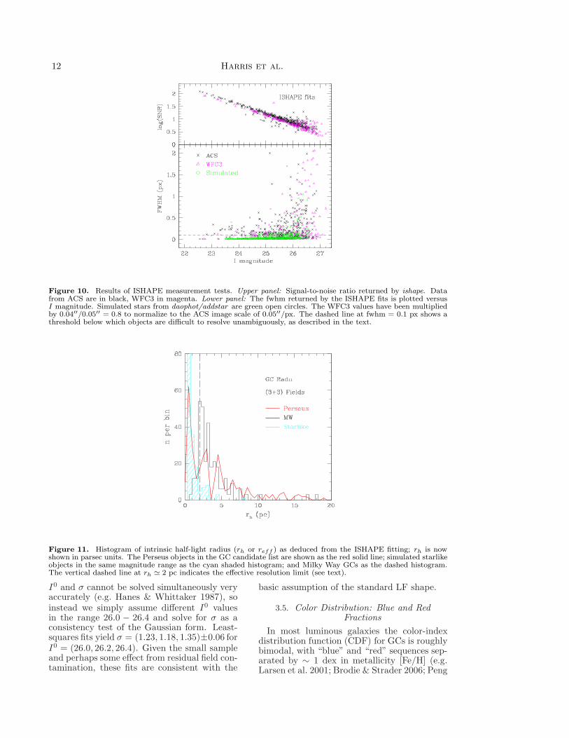
In Figure 11 the same data are displayedin histogram form, now converted to half-lightradii in parsec units. For a standard KING30model, rh = 1.48fwhm. Only the high-qualityGC candidates as defined above, with 22.5 <I < 26 and with 1.7 < (B − I) < 2.6, are in-cluded here. The distribution of Perseus GCsis clearly more extended than the (shaded)histogram for completely unresolved objects(i.e. simulated stars). For comparison the rhdistribution is shown for Milky Way clusters(Harris 1996, 2010 edition). To the extent al-lowed by the resolution limits of our imagingand the small sample sizes, the histograms forthe Milky Way and Perseus GCs agree quitewell.

3.4. Luminosity Function

Old GC populations consistently follow aGaussian-like luminosity function (LF) in num-ber per unit magnitude (e.g. Jordan et al. 2007;Villegas et al. 2010; Harris et al. 2014), so anadditional test of the nature of the Perseus can-didates is the shape of their LF. This is shownin Figure 12 for the combined candidate sam-ple. At present, only a very rough test can bemade again because of sample size. The pre-

vious work of HM17 shows similar results witha much bigger statistical sample, though theirdata include a higher fraction of GCs from thePerseus core galaxies.

The turnover (peak) absolute magnitude ofthe GCLF, and its dispersion σ have typicalvalues M0

I ≃ −8.3 and σ ≃ 1.3 for large galax-ies. However, both the turnover and disper-sion depend systematically on host galaxy lu-minosity (cf. Villegas et al. 2010) such thatlarger galaxies have progressively more lumi-nous turnovers (at the rate of ≃ 0.04 magper galaxy absolute magnitude) and broaderGCLFs (at the rate of ≃ 0.1 mag per galaxyabsolute magnitude). Recent modelling in-dicates that the biggest contributions to theICL are stars stripped from dwarf-sized tointermediate-sized galaxies (Harris et al. 2017a;Ramos-Almendares et al. 2018). Such galax-ies are 3 mag or more fainter than the gi-ants that much of the previous GCLF litera-ture has concentrated on. Thus in principle,accurate determination of the GCLF parame-ters for the ICGC component would providean additional observational test of its origin.With this in mind, we may expect very roughlyσ ∼ 1.0 and M0

I ∼ −8.2 or a turnover appar-ent magnitude I0 ≃ 26.4, almost half a mag-nitude fainter than the limit of our GC can-didate data. Under these circumstances, both

12 Harris et al.

Figure 10. Results of ISHAPE measurement tests. Upper panel: Signal-to-noise ratio returned by ishape. Datafrom ACS are in black, WFC3 in magenta. Lower panel: The fwhm returned by the ISHAPE fits is plotted versusI magnitude. Simulated stars from daophot/addstar are green open circles. The WFC3 values have been multipliedby 0.04′′/0.05′′ = 0.8 to normalize to the ACS image scale of 0.05′′/px. The dashed line at fwhm = 0.1 px shows athreshold below which objects are difficult to resolve unambiguously, as described in the text.

Figure 11. Histogram of intrinsic half-light radius (rh or reff ) as deduced from the ISHAPE fitting; rh is nowshown in parsec units. The Perseus objects in the GC candidate list are shown as the red solid line; simulated starlikeobjects in the same magnitude range as the cyan shaded histogram; and Milky Way GCs as the dashed histogram.The vertical dashed line at rh ≃ 2 pc indicates the effective resolution limit (see text).

I0 and σ cannot be solved simultaneously veryaccurately (e.g. Hanes & Whittaker 1987), soinstead we simply assume different I0 valuesin the range 26.0 − 26.4 and solve for σ as aconsistency test of the Gaussian form. Least-squares fits yield σ = (1.23, 1.18, 1.35)±0.06 forI0 = (26.0, 26.2, 26.4). Given the small sampleand perhaps some effect from residual field con-tamination, these fits are consistent with the

basic assumption of the standard LF shape.

3.5. Color Distribution: Blue and RedFractions

In most luminous galaxies the color-indexdistribution function (CDF) for GCs is roughlybimodal, with “blue” and “red” sequences sep-arated by ∼ 1 dex in metallicity [Fe/H] (e.g.Larsen et al. 2001; Brodie & Strader 2006; Peng

13

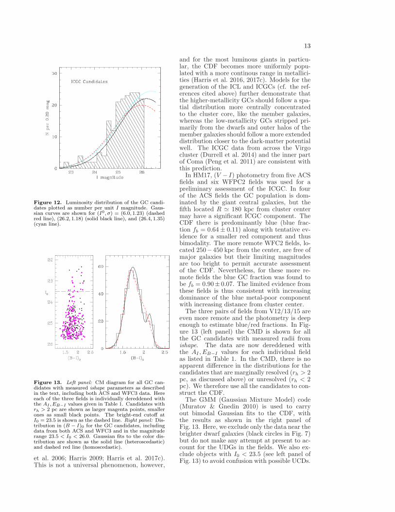
Figure 12. Luminosity distribution of the GC candi-dates plotted as number per unit I magnitude. Gaus-sian curves are shown for (I0, σ) = (6.0, 1.23) (dashedred line), (26.2, 1.18) (solid black line), and (26.4, 1.35)(cyan line).

Figure 13. Left panel: CM diagram for all GC can-didates with measured ishape parameters as describedin the text, including both ACS and WFC3 data. Hereeach of the three fields is individually dereddened withthe AI , EB−I values given in Table 1. Candidates withrh > 2 pc are shown as larger magenta points, smallerones as small black points. The bright-end cutoff atI0 = 23.5 is shown as the dashed line. Right panel: Dis-tribution in (B − I)0 for the GC candidates, includingdata from both ACS and WFC3 and in the magnituderange 23.5 < I0 < 26.0. Gaussian fits to the color dis-tribution are shown as the solid line (heteroscedastic)and dashed red line (homoscedastic).

et al. 2006; Harris 2009; Harris et al. 2017c).This is not a universal phenomenon, however,

and for the most luminous giants in particu-lar, the CDF becomes more uniformly popu-lated with a more continous range in metallici-ties (Harris et al. 2016, 2017c). Models for thegeneration of the ICL and ICGCs (cf. the ref-erences cited above) further demonstrate thatthe higher-metallicity GCs should follow a spa-tial distribution more centrally concentratedto the cluster core, like the member galaxies,whereas the low-metallicity GCs stripped pri-marily from the dwarfs and outer halos of themember galaxies should follow a more extendeddistribution closer to the dark-matter potentialwell. The ICGC data from across the Virgocluster (Durrell et al. 2014) and the inner partof Coma (Peng et al. 2011) are consistent withthis prediction.

In HM17, (V − I) photometry from five ACSfields and six WFPC2 fields was used for apreliminary assessment of the ICGC. In fourof the ACS fields the GC population is dom-inated by the giant central galaxies, but thefifth located R ≃ 180 kpc from cluster centermay have a significant ICGC component. TheCDF there is predominantly blue (blue frac-tion fb = 0.64 ± 0.11) along with tentative ev-idence for a smaller red component and thusbimodality. The more remote WFC2 fields, lo-cated 250− 450 kpc from the center, are free ofmajor galaxies but their limiting magnitudesare too bright to permit accurate assessmentof the CDF. Nevertheless, for these more re-mote fields the blue GC fraction was found tobe fb = 0.90± 0.07. The limited evidence fromthese fields is thus consistent with increasingdominance of the blue metal-poor componentwith increasing distance from cluster center.

The three pairs of fields from V12/13/15 areeven more remote and the photometry is deepenough to estimate blue/red fractions. In Fig-ure 13 (left panel) the CMD is shown for allthe GC candidates with measured radii fromishape. The data are now dereddened withthe AI , EB−I values for each individual fieldas listed in Table 1. In the CMD, there is noapparent difference in the distributions for thecandidates that are marginally resolved (rh > 2pc, as discussed above) or unresolved (rh < 2pc). We therefore use all the candidates to con-struct the CDF.

The GMM (Gaussian Mixture Model) code(Muratov & Gnedin 2010) is used to carryout bimodal Gaussian fits to the CDF, withthe results as shown in the right panel ofFig. 13. Here, we exclude only the data near thebrighter dwarf galaxies (black circles in Fig. 7)but do not make any attempt at present to ac-count for the UDGs in the fields. We also ex-clude objects with I0 < 23.5 (see left panel ofFig. 13) to avoid confusion with possible UCDs.

14 Harris et al.

With just n = 298 remaining datapoints afull heteroscedastic fit (unequal variances) isa bit risky, but making the assumption of un-equal variances we obtain a mean and standarddeviation µ1 = 1.743±0.017, σ1 = 0.178±0.011for the blue component and µ2 = 2.149 ±

0.027, σ2 = 0.062 ± 0.015 for the red compo-nent, with the blue GCs making up a fractionfb = 0.892 ± 0.043 of the total. These resultsare similar to the WFPC2 fields from HM17.Since ∆(B−I)/∆[Fe/H] = 0.39 (Barmby et al.2000; Harris et al. 2006), the color difference(µ2 − µ1) = 0.406 ± 0.032 between the red andblue modes corresponds to a metallicity differ-ence ∆[Fe/H] ≃ 1.0 dex, a normal value foundin most galaxies.

If we simplify the solution to a homosce-datic (equal variances) case, we obtain µ1 =1.682, µ2 = 2.007 with σ1 = σ2 = 0.146 andfb = 0.68. Requiring equal σ’s has the effect ofincreasing the red-mode variance and drawingit in to somewhat bluer color in order to matchthe CDF. Both of the solutions are shown inFig. 13. There is little to choose between them,but in both cases a unimodal CDF is rejectedwith > 99% confidence. At present, we con-clude only that the ICGCs in these quite re-mote fields show a CDF consistent with a rela-tively normal bimodal distribution; it is domi-nated by the metal-poor component but a smallmetal-richer component appears to be presentas well. More definite conclusions will have toawait samples from the other fields in our sur-vey.

4. SUMMARY

We describe the outline of our imaging pro-gram (PIPER) for the giant Perseus cluster ofgalaxies, with the HST ACS and WFC3 cam-eras. Exposures are designed to be deep enoughto reach almost to the LF turnover point of theglobular cluster systems in the Perseus galax-ies. Upon completion, the program will includephotometry in 35 different ACS or WFC3 fieldsextending from the cluster center (NGC 1275)out to projected radial distances more than 700kpc from center. The main goals for this pro-gram are to survey the globular cluster popula-tions around the giant galaxies in the Perseuscore, in 40 UDG candidates, and in the Intra-Cluster Medium, in addition to building a more

comprehensive sample of the UCDs and cEs inPerseus.

Data from the first three pointings of the pro-gram are presented here, along with an out-line of the photometric reduction methods usedto rigorously isolate GCs down to an effec-tive limiting magnitude I = 26 (MI = −8.6).These first results show that even at distancesR > 700 kpc, a sparse intergalactic popula-tion of GCs is clearly detectable, and evendominant over sources of field contamination.These ICGCs have magnitudes, color indices,linear sizes, and a luminosity distribution thatcomfortably match conventional GCs in nearbygalaxies. Stronger conclusions about all theseproperties await the completion of the obser-vational program. Once all the fields are inhand, an exciting prospect will be to gauge thespatial distribution of the ICGC and the radialchange in its metallicity distribution, leading toa stronger link with models for the origin of theICL.

In future papers of this series, analyses willconcentrate on the UDGs and their own GCpopulations, the central giant galaxies, and theUCDs and compact ellipticals to be discoveredin our target fields.

WEH acknowledges financial support fromNSERC (Natural Sciences and Engineering Re-search Council of Canada). AJR was supportedby National Science Foundation grant AST-1515084 and as a Research Corporation forScience Advancement Cottrell Scholar. AJRand PRD are supported by funds providedby NASA through grant GO-15235 from theSpace Telescope Science Institute, which is op-erated by the Association of Universities forResearch in Astronomy, Incorporated, underNASA contract NAS5-26555. CW and TLare supported by the Deutsche Forschungsge-meinschaft (DFG, German Research Founda-tion) through project 394551440. TL acknowl-edges financial support from the EuropeanUnion’s Horizon 2020 research and innovationprogramme under the Marie Sk lodowska-Curiegrant agreement No. 721463 to the SUNDIALITN network.

HST (ACS, WFC3)

REFERENCES

Alamo-Martınez, K. A. & Blakeslee, J. P. 2017, ApJ,849, 6

Amorisco, N. C., Monachesi, A., Agnello, A., & White,S. D. M. 2018, MNRAS, 475, 4235

Barmby, P., Huchra, J. P., Brodie, J. P., Forbes,D. A., Schroder, L. L., & Grillmair, C. J. 2000, AJ,119, 727

Beasley, M. A. & Trujillo, I. 2016, ApJ, 830, 23

Bertin, E. & Arnouts, S. 1996, A&AS, 117, 393Brodie, J. P. & Strader, J. 2006, ARA&A, 44, 193Burke, C., Collins, C. A., Stott, J. P., & Hilton, M.

2012, MNRAS, 425, 2058

15

Canning, R. E. A., Ryon, J. E., Gallagher, J. S.,Kotulla, R., O’Connell, R. W., Fabian, A. C.,Johnstone, R. M., Conselice, C. J., Hicks, A.,Rosario, D., & Wyse, R. F. G. 2014, MNRAS, 444,336

Colless, M. & Dunn, A. M. 1996, ApJ, 458, 435Deustua, S. E. & Mack, J. 2018, Comparing the

ACS/WFC and WFC3/UVIS Calibration andPhotometry, Tech. rep.

Durrell, P. R., Cote, P., Peng, E. W., Blakeslee, J. P.,Ferrarese, L., Mihos, J. C., Puzia, T. H., Lancon, A.,Liu, C., Zhang, H., Cuillandre, J.-C., McConnachie,A., Jordan, A., Accetta, K., Boissier, S., Boselli, A.,Courteau, S., Duc, P.-A., Emsellem, E., Gwyn, S.,Mei, S., & Taylor, J. E. 2014, ApJ, 794, 103

El-Badry, K., Quataert, E., Weisz, D. R., Choksi, N.,& Boylan-Kolchin, M. 2018, ArXiv e-prints

Fabian, A. C., Sanders, J. S., Allen, S. W., Canning,R. E. A., Churazov, E., Crawford, C. S., Forman,W., Gabany, J., Hlavacek-Larrondo, J., Johnstone,R. M., Russell, H. R., Reynolds, C. S., Salome, P.,Taylor, G. B., & Young, A. J. 2011, MNRAS, 418,2154

Ferre-Mateu, A., Forbes, D. A., Romanowsky, A. J.,Janz, J., & Dixon, C. 2018, MNRAS, 473, 1819

Georgiev, I. Y., Goudfrooij, P., Puzia, T. H., & Hilker,M. 2008, AJ, 135, 1858

Girardi, L., Groenewegen, M. A. T., Hatziminaoglou,E., & da Costa, L. 2005, A&A, 436, 895

Girardi, M., Fadda, D., Giuricin, G., Mardirossian, F.,Mezzetti, M., & Biviano, A. 1996, ApJ, 457, 61

Girardi, M., Giuricin, G., Mardirossian, F., Mezzetti,M., & Boschin, W. 1998, ApJ, 505, 74

Hanes, D. A. & Whittaker, D. G. 1987, AJ, 94, 906Harris, K. A., Debattista, V. P., Governato, F.,

Thompson, B. B., Clarke, A. J., Quinn, T.,Willman, B., Benson, A., Farrah, D., Peng, E. W.,Elliott, R., & Petty, S. 2017a, MNRAS, 467, 4501

Harris, W. E. 1996, AJ, 112, 1487—. 2009, ApJ, 699, 254Harris, W. E., Blakeslee, J. P., & Harris, G. L. H.

2017b, ApJ, 836, 67Harris, W. E., Blakeslee, J. P., Whitmore, B. C.,

Gnedin, O. Y., Geisler, D., & Rothberg, B. 2016,ApJ, 817, 58

Harris, W. E., Ciccone, S. M., Eadie, G. M., Gnedin,O. Y., Geisler, D., Rothberg, B., & Bailin, J. 2017c,ApJ, 835, 101

Harris, W. E., Morningstar, W., Gnedin, O. Y.,O’Halloran, H., Blakeslee, J. P., Whitmore, B. C.,Cote, P., Geisler, D., Peng, E. W., Bailin, J.,Rothberg, B., Cockcroft, R., & Barber DeGraaff, R.2014, ApJ, 797, 128

Harris, W. E. & Mulholland, C. J. 2017, ApJ, 839, 102Harris, W. E., Whitmore, B. C., Karakla, D., Okon,

W., Baum, W. A., Hanes, D. A., & Kavelaars, J. J.2006, ApJ, 636, 90

Haynes, M. P. & Giovanelli, R. 1986, ApJ, 306, L55Hinshaw, G., Larson, D., Komatsu, E., Spergel, D. N.,

Bennett, C. L., Dunkley, J., Nolta, M. R., Halpern,M., Hill, R. S., Odegard, N., Page, L., Smith, K. M.,Weiland, J. L., Gold, B., Jarosik, N., Kogut, A.,Limon, M., Meyer, S. S., Tucker, G. S., Wollack, E.,& Wright, E. L. 2013, ApJS, 208, 19

Hudson, M. J., Harris, G. L., & Harris, W. E. 2014,ApJ, 787, L5

Janssens, S., Abraham, R., Brodie, J., Forbes, D.,Romanowsky, A. J., & van Dokkum, P. 2017, ApJ,839, L17

Janz, J., Norris, M. A., Forbes, D. A., Huxor, A.,Romanowsky, A. J., Frank, M. J., Escudero, C. G.,Faifer, F. R., Forte, J. C., Kannappan, S. J.,Maraston, C., Brodie, J. P., Strader, J., &Thompson, B. R. 2016, MNRAS, 456, 617

Jordan, A., McLaughlin, D. E., Cote, P., Ferrarese, L.,Peng, E. W., Mei, S., Villegas, D., Merritt, D.,Tonry, J. L., & West, M. J. 2007, ApJS, 171, 101

Kent, S. M. & Sargent, W. L. W. 1983, AJ, 88, 697Koda, J., Yagi, M., Yamanoi, H., & Komiyama, Y.

2015, ApJ, 807, L2Larsen, S. S. 1999, A&AS, 139, 393Larsen, S. S., Brodie, J. P., Huchra, J. P., Forbes,

D. A., & Grillmair, C. J. 2001, AJ, 121, 2974Lim, S., Peng, E. W., Cote, P., Sales, L. V., den Brok,

M., Blakeslee, J. P., & Guhathakurta, P. 2018,ArXiv e-prints

Loewenstein, M. 1994, ApJ, 431, 91Lotz, J. M., Koekemoer, A., Coe, D., Grogin, N.,

Capak, P., Mack, J., Anderson, J., Avila, R., Barker,E. A., Borncamp, D., Brammer, G., Durbin, M.,Gunning, H., Hilbert, B., Jenkner, H., Khandrika,H., Levay, Z., Lucas, R. A., MacKenty, J., Ogaz, S.,Porterfield, B., Reid, N., Robberto, M., Royle, P.,Smith, L. J., Storrie-Lombardi, L. J., Sunnquist, B.,Surace, J., Taylor, D. C., Williams, R., Bullock, J.,Dickinson, M., Finkelstein, S., Natarajan, P.,Richard, J., Robertson, B., Tumlinson, J., Zitrin,A., Flanagan, K., Sembach, K., Soifer, B. T., &Mountain, M. 2017, ApJ, 837, 97

Main, R. A., McNamara, B. R., Nulsen, P. E. J.,Russell, H. R., & Vantyghem, A. N. 2017, MNRAS,464, 4360

Martınez-Delgado, D., Lasker, R., Sharina, M.,Toloba, E., Fliri, J., Beaton, R., Valls-Gabaud, D.,Karachentsev, I. D., Chonis, T. S., Grebel, E. K.,Forbes, D. A., Romanowsky, A. J.,Gallego-Laborda, J., Teuwen, K., Gomez-Flechoso,M. A., Wang, J., Guhathakurta, P., Kaisin, S., &Ho, N. 2016, AJ, 151, 96

Martinovic, N. & Micic, M. 2017, MNRAS, 470, 4015Matsushita, K., Sakuma, E., Sasaki, T., Sato, K., &

Simionescu, A. 2013, ApJ, 764, 147Mieske, S., Hilker, M., & Misgeld, I. 2012, A&A, 537,

A3Muratov, A. L. & Gnedin, O. Y. 2010, ApJ, 718, 1266Papastergis, E., Adams, E. A. K., & Romanowsky,

A. J. 2017, A&A, 601, L10Peng, E. W., Ferguson, H. C., Goudfrooij, P.,

Hammer, D., Lucey, J. R., Marzke, R. O., Puzia,T. H., Carter, D., Balcells, M., Bridges, T.,Chiboucas, K., del Burgo, C., Graham, A. W.,Guzman, R., Hudson, M. J., Matkovic, A., Merritt,D., Miller, B. W., Mouhcine, M., Phillipps, S.,Sharples, R., Smith, R. J., Tully, B., & VerdoesKleijn, G. 2011, ApJ, 730, 23

Peng, E. W., Jordan, A., Cote, P., Blakeslee, J. P.,Ferrarese, L., Mei, S., West, M. J., Merritt, D.,Milosavljevic, M., & Tonry, J. L. 2006, ApJ, 639, 95

Peng, E. W. & Lim, S. 2016, ApJ, 822, L31Penny, S. J., Conselice, C. J., de Rijcke, S., Held,

E. V., Gallagher, J. S., & O’Connell, R. W. 2011,MNRAS, 410, 1076

Penny, S. J., Forbes, D. A., & Conselice, C. J. 2012,MNRAS, 422, 885

Pfeffer, J., Griffen, B. F., Baumgardt, H., & Hilker, M.2014, MNRAS, 444, 3670

Ramos, F., Coenda, V., Muriel, H., & Abadi, M. 2015,ApJ, 806, 242

Ramos-Almendares, F., Abadi, M., Muriel, H., &Coenda, V. 2018, ApJ, 853, 91

Roman, J. & Trujillo, I. 2017, MNRAS, 468, 4039

16 Harris et al.

Simionescu, A., Allen, S. W., Mantz, A., Werner, N.,Takei, Y., Morris, R. G., Fabian, A. C., Sanders,J. S., Nulsen, P. E. J., George, M. R., & Taylor,G. B. 2011, Science, 331, 1576

Sirianni, M., Jee, M. J., Benıtez, N., Blakeslee, J. P.,Martel, A. R., Meurer, G., Clampin, M., De Marchi,G., Ford, H. C., Gilliland, R., Hartig, G. F.,Illingworth, G. D., Mack, J., & McCann, W. J.2005, PASP, 117, 1049

Struble, M. F. & Rood, H. J. 1991, ApJS, 77, 363Toloba, E., Lim, S., Peng, E., Sales, L. V.,

Guhathakurta, P., Mihos, J. C., Cote, P., Boselli, A.,Cuillandre, J.-C., Ferrarese, L., Gwyn, S., Lancon,A., Munoz, R., & Puzia, T. 2018, ApJ, 856, L31

van Dokkum, P., Abraham, R., Brodie, J., Conroy, C.,Danieli, S., Merritt, A., Mowla, L., Romanowsky,A., & Zhang, J. 2016, ApJ, 828, L6

van Dokkum, P., Cohen, Y., Danieli, S., Kruijssen,J. M. D., Romanowsky, A. J., Merritt, A., Abraham,R., Brodie, J., Conroy, C., Lokhorst, D., Mowla, L.,O’Sullivan, E., & Zhang, J. 2018, ApJ, 856, L30

van Dokkum, P. G., Abraham, R., Merritt, A., Zhang,J., Geha, M., & Conroy, C. 2015a, ApJ, 798, L45

van Dokkum, P. G., Romanowsky, A. J., Abraham,R., Brodie, J. P., Conroy, C., Geha, M., Merritt, A.,Villaume, A., & Zhang, J. 2015b, ApJ, 804, L26

Villegas, D., Jordan, A., Peng, E. W., Blakeslee, J. P.,Cote, P., Ferrarese, L., Kissler-Patig, M., Mei, S.,Infante, L., Tonry, J. L., & West, M. J. 2010, ApJ,717, 603

Voggel, K. T., Seth, A. C., Neumayer, N., Mieske, S.,Chilingarian, I., Ahn, C., Baumgardt, H., Hilker,M., Nguyen, D. D., Romanowsky, A. J., Walsh,J. L., den Brok, M., & Strader, J. 2018, ApJ, 858, 20

Wegner, G., Haynes, M. P., & Giovanelli, R. 1993, AJ,105, 1251

Weinmann, S. M., Lisker, T., Guo, Q., Meyer, H. T.,& Janz, J. 2011, MNRAS, 416, 1197

West, M. J., Jordan, A., Blakeslee, J. P., Cote, P.,Gregg, M. D., Takamiya, M., & Marzke, R. O. 2011,A&A, 528, A115

Wittmann, C., Lisker, T., Ambachew Tilahun, L.,Grebel, E. K., Conselice, C. J., Penny, S., Janz, J.,Gallagher, J. S., Kotulla, R., & McCormac, J. 2017,MNRAS, 470, 1512

Wittmann, C., Lisker, T., Pasquali, A., Hilker, M., &Grebel, E. K. 2016, MNRAS, 459, 4450

Zhang, Y. & Bell, E. F. 2017, ApJ, 835, L2Zhao, H.-H., Jia, S.-M., Chen, Y., Li, C.-K., Song,

L.-M., & Xie, F. 2013, ApJ, 778, 124