Ple

ase

note

that

this

is a

n au

thor

-pro

duce

d P

DF

of a

n ar

ticle

acc

ept

ed fo

r pu

blic

atio

n fo

llow

ing

peer

rev

iew

. The

def

initi

ve p

ub

lish

er-a

uthe

ntic

ated

ve

rsio

n is

ava

ilab

le o

n th

e pu

blis

her

Web

site

1

Deep Sea Research Part I: Oceanographic Research Papers October 2009, Volume 56, Issue 10, Pages 1615-163 http://dx.doi.org/10.1016/j.dsr.2009.06.002 © 2009 Elsevier Ltd All rights reserved.

Archimer Archive Institutionnelle de l’Ifremer

http://www.ifremer.fr/docelec/

The mid-depth circulation of the northwestern tropical Atlantic observed by floats

Matthias Lankhorsta, d, *, David Fratantonib, Michel Ollitraultc, Philip Richardsonb, Uwe Senda, d

and Walter Zenka a Leibniz-Institut für Meereswissenschaften (IFM-GEOMAR), Kiel, Germany b Woods Hole Oceanographic Institution (WHOI), Woods Hole, MA, USA c Institut français de recherche pour l’exploitation de la mer (Ifremer), Plouzané, France d Scripps Institution of Oceanography (SIO), 9500 Gilman Drive, Mail code 0230, La Jolla, CA 92093-0230, USA *: Corresponding author : Matthias Lankhorst, email address : mlankhorst@ucsd.edu

Abstract: A comprehensive analysis of velocity data from subsurface floats in the northwestern tropical Atlantic at two depth layers is presented: one representing the Antarctic Intermediate Water (AAIW, pressure range 600–1050 dbar), the other the upper North Atlantic Deep Water (uNADW, pressure range 1200–2050 dbar). New data from three independent research programs are combined with previously available data to achieve blanket coverage in space for the AAIW layer, while coverage in the uNADW remains more intermittent. Results from the AAIW mainly confirm previous studies on the mean flow, namely the equatorial zonal and the boundary currents, but clarify details on pathways, mostly by virtue of the spatial data coverage that sets float observations apart from e.g. shipborne or mooring observations. Mean transports in each of five zonal equatorial current bands is found to be between 2.7 and 4.5 Sv. Pathways carrying AAIW northward beyond the North Brazil Undercurrent are clearly visible in the mean velocity field, in particular a northward transport of 3.7 Sv across 16°N between the Antilles islands and the Mid-Atlantic Ridge. New maps of Lagrangian eddy kinetic energy and integral time scales are presented to quantify mesoscale activity. For the uNADW, mean flow and mesoscale properties are discussed as data availability allows. Trajectories in the uNADW east of the Lesser Antilles reveal interactions between the Deep Western Boundary Current (DWBC) and the basin interior, which can explain recent hydrographic observations of changes in composition of DWBC water along its southward flow. Keywords: Floats; Tropical Atlantic; Antarctic Intermediate Water; North Atlantic Deep Water; Equatorial currents

1 Introduction24

This paper considers the area of the open Atlantic Ocean north of 10◦ S and south of25

the tropic of cancer (23.5◦ N), between 65◦ W and 30◦ W, which we will refer to as the26

northwestern tropical Atlantic. The island chain of the eastern Lesser Antilles and the27

coast of South America limit the domain in the west and southwest, whereas the other28

boundaries are in the open ocean. Parts of the Mid-Atlantic Ridge cross the domain29

and, together with the American coastline, define a diagonal sub-basin aligned from the30

northwest to the southeast that is characteristic of the region. Fig. 1 (top panel) shows a31

map of the area that includes the geographic features referred to in the text. The middle32

and bottom panels show the spatial data coverage.33

Two depth ranges will be considered: one represents the Antarctic Intermediate Wa-34

ter (AAIW), and the other the upper part of the North Atlantic Deep Water (NADW).35

The motivation for studying the circulation of the Atlantic at these depths is the involve-36

ment of the currents in the Meridional Overturning Circulation (MOC). The Atlantic37

MOC carries relatively warm water northward near the surface and cold water southward38

at depth. The resulting northward heat transport is seen as an important part of the39

climate system (Marshall et al., 2001). AAIW with its northward spreading is associated40

with the upper limb of the MOC, while NADW is the southward component. This study41

was initiated as a synergy of three field experiments with subsurface floats that drift with42

the surrounding water: MOVE1 originally based at IFM-GEOMAR, NBC2 Rings Exper-43

iment based at WHOI, and SAMBA3 based at Ifremer. The main objective of MOVE is44

monitoring the southward transport of NADW east of the lesser Antilles with moored sen-45

sors (Send et al., 2002). Floats were deployed to assist the interpretation of the mooring46

1Meridional Overturning and Variability Experiment2North Brazil Current3Sub-Antarctic Motions in the Brazil Basin

2

measurements in the early phase of the experiment. The NBC Rings Experiment inves-47

tigated the NBC off of South America between roughly 5◦ N and 10◦ N (Fratantoni and48

Richardson, 2006). The main constituent of the upper limb of the MOC, the NBC carries49

waters in the upper 1000 m northward across the equator and sheds anticyclonic current50

rings in its retroflection (Johns et al., 2003). SAMBA intends to map out the circulation51

of the AAIW in the Brazil Basin with a large amount of floats, some of which are within52

the domain of this study. The areas where data were gathered in these three campaigns53

complement each other to span almost the entire northwestern tropical Atlantic. Pub-54

licly available float data from five other field campaigns were added to further enlarge55

the database (listed in table 2). The total data amount is 305 cumulative years of float56

data, and the largest individual contributing project is now Argo. None of the individual57

projects by itself except perhaps Argo in the near future is capable of a basin-wide treat-58

ment of the circulation at the resolution required to map out the relatively narrow current59

bands. The combination of multiple datasets makes this possible for the AAIW layer. Pre-60

vious observations of the circulation patterns (e. g. Stramma and Schott, 1999) are based61

mostly on mooring or shipborne observations of velocity, which lack spatial resolution,62

or hydrographic and tracer observations, which are powerful yet only indirect measures63

of the circulation. Float observations can fill these gaps with area-wide direct velocity64

observations, and studies of the tropical Atlantic with floats by Boebel et al. (1999a) and65

Schmid et al. (2003) have shown updated schematics of the circulation. However, these66

were based on relatively small amounts of data, especially in the northwestern tropical67

Atlantic, which is addressed here. This paper mostly confirms the previous circulation68

schematics with estimates of the mean flow that are based on substantially improved data69

coverage, supported by pathways visible in a multitude of individual trajectories. From70

eddy-resolving float data, kinetic energy levels and time scales of the mesoscale field are71

presented. As for the uNADW layer, data coverage remains limited. Older SOFAR float72

3

data that have been discussed in the literature (Richardson and Schmitz, 1993; Richardson73

and Fratantoni, 1999) are included in this study, but the discussion focuses on new data74

east of the Lesser Antilles, which are brought into context with recent hydrographic ob-75

servations by Steinfeldt et al. (2007). Where possible, mean flow and mesoscale properties76

are quantified for the uNADW layer as well.77

AAIW is formed in subpolar regions around Antarctica, from where it is subducted78

and spreads throughout the South Atlantic (Talley, 1996; Stramma and England, 1999).79

Its most conspicuous path is along the shelf break off South America between roughly80

27◦ S and 10◦ N in the aforementioned North Brazil (Under-) Current (NBC, NBUC,81

Stramma et al., 1995), also called the Intermediate Western Boundary Current (IWBC).82

Near the equator, the path of AAIW is complicated by bands of alternating zonal flow,83

which have been described by Ollitrault et al. (2006) in a precursor to this study, and84

earlier e. g. by Schmid et al. (2003). Stramma et al. (2005) present ship-based measure-85

ments within the domain that include data in the AAIW, and Boebel et al. (1999b) give86

a comprehensive account of the intermediate-depth equatorial currents in the earlier liter-87

ature. The situation within 1◦ of the equator is complicated by vertically alternating jets88

(e. g. Gouriou et al., 2001; Send et al., 2002; Schmid et al., 2005), the dynamics of which89

are not yet well understood. Fig. 1 (middle) schematically shows locations and directions90

of the NBUC and five equatorial current bands: the Northern and Southern Equatorial91

Intermediate Currents (NEIC, SEIC) flowing westward near 4◦ N/S, the Northern and92

Southern Intermediate Countercurrents (NICC, SICC) flowing eastward near 2◦ N/S, and93

the Equatorial Intermediate Current (EIC) flowing westward on average at the equator94

(seasonal cycles and reversals described e. g. by Ollitrault et al., 2006).95

The main hydrographic characteristic of AAIW is a minimum in vertical salinity pro-96

files, shown in fig. 2 with velocities from an LADCP (Lowered Acoustic Doppler Current97

Profiler) on two sections (data from Rhein et al., 2004, 2005). Current features captured98

4

by the LADCP data include the NBC, NEIC, NICC, EIC, SICC, and an eddy that Rhein99

et al. (2005) identify as an NBC ring. The minimum in salinity can be identified through100

the entire study domain, although its northern extent does not reach far beyond the trop-101

ics (e. g. Talley, 1996). Here, floats drifting at pressures between 600 and 1050 dbar will102

be interpreted as being in the AAIW. This choice agrees with the isopycnals shown in103

fig. 2, which in turn are used by Stramma and England (1999) and Rhein et al. (1995),104

although it includes upper Circumpolar Deep Water which is between approximately 900105

and 1100 dbar.106

In contrast to AAIW, NADW as a whole stems from convection and mixing processes107

in the polar and subpolar North Atlantic. Following the North American shelf break108

southward, it reaches the tropics as a Deep Western Boundary Current (DWBC, cf. figs.109

1 (bottom) and 2), where it occupies pressure ranges between approximately 1200 and110

3900 dbar (Rhein et al., 1995). More specifically, we will combine floats in the range111

1200–2050 dbar as being in the upper NADW (uNADW), a common naming convention112

used e. g. by Curry et al. (1998, for more details, see Rhein et al. (1995)). In hydrographic113

measurements, this depth range is characterized by the highest salinity of the NADW (fig.114

2). NADW too is subject to zonal current bands away from the DWBC in the equatorial115

region (Richardson and Fratantoni, 1999).116

A current review of float technology, including all types of instrumentation exploited117

here, is given by Rossby (2007). Two positioning strategies have evolved for floats: acous-118

tic floats are positioned acoustically while submerged, and profiling floats return to the119

surface periodically for satellite position fixes. Currents are derived from the displace-120

ments between successive fixes. Here, acoustic floats have one or two position fixes per121

day, which makes them eddy-resolving. Profiling floats, in contrast, are located typically122

every ten days and therefore do not resolve the mesoscale, but the larger number of them123

helps to map out the mean flow. Mean currents are derived from combining displacements124

5

between individual cycles of profiling floats, and acoustic trajectories sub-sampled at ten-125

day intervals. The discussion of mesoscale variability is based on acoustic floats only.126

Typical eddy time scales will be shown to be shorter than ten days, so that successive127

float displacement cycles can be assumed statistically independent.128

2 Mean Flow Field129

2.1 Mean Flow Derived from Float Observations130

2.1.1 Antarctic Intermediate Water (AAIW)131

Fig. 3 shows a stream function derived from all available float displacements in the AAIW132

layer. The individual velocity measurements shown in fig. 1b were interpolated onto a133

grid of 0.5◦ resolution, with Gaussian weights of standard deviation 50 km. From these134

gridpoints, vorticity ζ was derived by central differences, and the stream function Ψ was135

obtained by numerically solving4 the Poisson equation ∇2Ψ = −ζ on the domain136

shown in the figure. The boundary condition along the American shelf is a constant137

streamline (Dirichlet boundary condition), while the boundary conditions in the open138

ocean are defined through the velocity measurements themselves (Neumann boundary139

conditions). All flow features discussed below are also present in the raw gridded velocity140

data and therefore not artefacts of the streamline computation.141

The resulting stream function clearly depicts the NBUC and the following five equa-142

torial zonal flows as the features with the strongest currents: NEIC, NICC, EIC, SICC,143

and SEIC. The equatorial zonal flows have been discussed by Ollitrault et al. (cf. 2006).144

Assuming a layer thickness of 450 m, the mean volume transports of the five equatorial145

4MatLabTM contains the algorithms in its “PDE toolbox” product.

6

currents in the middle of the basin (longitudes from 40◦ W for the NEIC to 30◦ W for146

the SEIC) are approximately 3.2, 4.5, 3.2, 4.1, and 2.7 Sv, respectively. Until recently,147

there has been doubt about the mere existence of these intermediate-depth zonal flows148

(Jochum and Malanotte-Rizzoli, 2003), which has been eliminated by successive observa-149

tional (Schott et al., 2003; Schmid et al., 2003) and modelling studies (Eden, 2006). The150

positions of the NEIC and to some extent the NICC shift northward at short distances151

from the western boundary, in the case of the NEIC from near 4◦ N in the basin interior to152

5◦ N at 45◦ W. This shifted NEIC location is not reproduced by Schmid et al. (2003, their153

fig. 17). Stramma and Schott (1999, their fig. 6) generally show the NEIC too far north.154

The streamlines of the NICC and NEIC in these displacements (west of 40◦ W) tend to155

follow the deep isobaths of the Ceara Ridge and the Amazon Cone, suggesting that these156

topographic features exert some guidance on the AAIW flow although they are at depths157

exceeding 3000 m. At least it seems likely that the NEIC would continue along 4◦ N all158

the way to the western boundary if the ridge were not there. The inflow in the NBUC159

at 8◦ S is found to be 5.0 Sv, which is in general agreement with the analysis by Schott160

et al. (1998). All transport values were obtained by integrating across the streamlines of161

fig. 3 and are listed in table 3 together with previous estimates.162

Northwestward from the Guiana Plateau, the streamlines suggest a continuous flow163

of AAIW parallel to but mostly detached from the shelf break. This mean flow is not easily164

observed due to masking by the mesoscale eddy field (discussed in section 3), yet it seems165

to be the major pathway of AAIW west of 53◦ W. From the Guiana Plateau to Barbados,166

this path resembles the advection of NBC rings (Fratantoni and Richardson, 2006; Johns167

et al., 2003; Goni and Johns, 2001). Consistent with these studies on NBC rings, which168

repeatedly show rings near or even around Barbados, fig. 3 shows northward flow to either169

side of the island with a larger portion west of it as would be expected of an anticyclone170

surrounding Barbados as it progresses northward. At 15◦ N north of Barbados, some171

7

northward flow remains close to but not as tightly concentrated at the boundary, while172

four streamlines fan out northeastward into the ocean interior. The location coincides173

with one where many NBC rings stall or cease to exist (Fratantoni and Richardson, 2006;174

Goni and Johns, 2001). Stalling of the rings can explain why hydrographic measurements175

(Rhein et al., 2005, or fig. 2 here) repeatedly find them there, and why the mean flow176

decelerates as documented by the fanning out of the streamlines. The separation of the177

streamlines from the western boundary at 15◦ N is also consistent with the hydrography,178

which shows the thickest layer of fresher water (fig. 2) or the highest concentrations179

of water from the southern hemisphere (Rhein et al., 2005) beginning at least 200 km180

offshore. In their analysis of water entering the Caribbean between the Lesser Antilles,181

Rhein et al. (2005) identify higher concentrations of southern waters in passages between182

the islands south of 15◦ N, exactly where fig. 3 here finds the mean flow—presumably183

carrying the highest concentrations of AAIW—closer to the islands than it does further184

north. Northward transports across 16◦ N are 1.4 Sv in the interior pathway (east of185

59◦ W but west of the Mid-Atlantic Ridge) and 2.3 Sv in the path closer to the boundary.186

Assuming that transport across 16◦ N happens by advection of remaining NBC rings,187

Rhein et al. (2005) derive a transport that agrees with these values (see table 3). We188

therefore interpret the mean flow in the AAIW layer from the Guiana Plateau onward189

as the translation of NBC rings, a concept introduced by Richardson et al. (1994) for190

near-surface data. At the northern limit of the domain (beyond 20◦ N), the wider spacing191

of the streamlines and associated low speeds correspond with the northernmost extent of192

the salinity minimum of AAIW (e. g. Talley, 1996, or WOCE5 section A20).193

The remaining area apart from the equatorial and boundary regimes is characterized194

by very slow—if any—mean flow. Stramma and Schott (1999) have presented a circulation195

schematic of the entire tropical Atlantic for the AAIW layer (their fig. 6), based on196

5Cf. e. g. http://www.ewoce.org

8

measurements available then, i. e. before the availability of large float data amounts.197

Excellent agreement with respect to the equatorial and near-equatorial flow (EIC, NICC,198

SICC) is found between our fig. 3 and the schematic by Stramma and Schott (1999).199

However, they display the NEIC further north, and the SEIC is obscured in several200

branches of the South Equatorial Current and the mostly shallower South Equatorial201

Undercurrent. Their continued northward flow beyond the NBUC, which they refer to as202

the IWBC, enters the Caribbean between the southernmost Antilles islands, unlike what203

floats show here, and they show large inter-basin gyres between 5◦ and 20◦ N where float204

data suggest insignificant mean flow. With the IWBC escaping into the Caribbean, their205

scheme cannot reproduce the flow towards Barbados and further north. Some of these206

discrepancies in the equatorial region, approximately 8◦ S to 5◦ N, have been clarified in a207

similar schematic by Schmid et al. (2003, their fig. 17) based on float data included in this208

study. Schmid et al. (2003) adjust the position of the NEIC and simplify the zonal flow209

patterns around the SEIC to a degree that matches the findings presented here, although210

they rely on individual trajectories in some cases. However, they continue to include211

parts of an inter-basin, anticyclonic gyre north of the NEIC, which is not supported by212

the present study. We will update the schematics by Stramma and Schott (1999) and213

Schmid et al. (2003) in the conclusions at the end of the paper.214

2.1.2 Upper North Atlantic Deep Water (uNADW)215

Data density of the uNADW layer does not allow for a similar map of streamlines, but216

fig. 4 shows box-averaged mean velocities where data are available. Near the DWBC, the217

boxes were designed to follow the flow features as seen in individual trajectories (cf. fig. 9).218

In a broad area east of the Lesser Antilles (between 11◦ N and 19◦ N, 58◦ W and 46◦ W),219

there is slow but prevalent westward mean flow of 0.8 cm s−1 with a standard error of220

0.2 cm s−1. For a subset of this data (MOVE), the mean flow is even higher at 1.5 cm s−1221

9

with the same standard error. This westward flow comes at least from near the Mid-222

Atlantic Ridge, possibly from further east, and connects with the southward DWBC near223

the Lesser Antilles. Steinfeldt et al. (2007) find a strong dilution of the DWBC between224

16◦ N and 10◦ N based on tracer measurements, which can be explained by this inflow225

from the east. The origin of this westward flow is not obvious from the present dataset,226

but NADW has been observed to spread southward east of the Mid-Atlantic Ridge at227

latitudes between 35◦ N and 50◦ N (Speer et al., 1999; Bower et al., 2002; Machın et al.,228

2006). In the same latitudinal range, Paillet et al. (1998) and Getzlaff et al. (2006) discuss229

a southward path along the ridge. Hence we speculate that the westward flow observed230

by the floats is fed by a branch of uNADW that does not spread in the DWBC but rather231

via slower pathways along or east of the Mid-Atlantic Ridge.232

Centered at about 15◦ N at the western boundary of the domain, a narrow recircu-233

lation cell is also present in the mean, which could be yet another reason for the dilution234

observed by Steinfeldt et al. (2007). Results from the SOFAR floats off South America,235

which have measured the boundary current and parts of the equatorial current system,236

have been published by Richardson and Fratantoni (1999) but are not well represented in237

fig. 4 due to data sparsity.238

2.2 Comparison with Other Measurements239

Several measurements with moored current meters exist in the study area with instru-240

ments within the AAIW and the uNADW layers. An overview of the locations of these241

moorings is included in fig. 1. Figures 5 and 6 show comparisons of mean velocities be-242

tween float and mooring data across three sections. The sections were designed to be243

perpendicular to the shelf break. Float data within 167 km (1.5◦) to either side of the244

target sections (within 222 km or 2◦ for the two southern uNADW sections) are used245

10

to compute across-section velocities. Float data are grouped into bins of 100 km width,246

and the figures show the bin averages, 95% confidence limits, and the scattered cloud247

of individual float samples. Means and confidence intervals from moored sensors are248

superimposed. In all sections, the boundary currents are the most prominent features.249

Here, agreement between mooring and float data is probed to rebut the suspicion that250

interpretation of float data is flawed by systematic deviations between the two (Stokes251

Drift).252

Fig. 5 shows results on the AAIW. Near the endpoints of the northernmost section253

(a), multi-year mooring records from MOVE and float data concordantly show zero mean254

flow. Mooring data from Johns et al. (1990, section b) show the northwestward NBUC255

with mean currents near 13 cm s−1 at the boundary, decreasing to almost zero 150 km256

out, in excellent agreement with the float data. Section (c) contains mooring data from257

Schott et al. (1993), which show a northwestward NBUC flanked by a southeastward258

flow. The float averages show the same features, generally with a stronger northwestward259

component, and disagreements are within the confidence limits. Section (c) in particular260

highlights how the basin-wide float coverage adds to the interpretation of the existing261

data, since the floats reveal the southeastward flow seen in the mooring data to be part262

of the alternating pattern of zonal flows in the equatorial region (the NICC in this case).263

The streamlines of fig. 3 (included in fig. 5) show how the NBUC flow at section (c) folds264

back in the NICC, is then re-established at section (b), and successively detrained in a265

recirculation within the Guiana Basin as well as fanned out away from the coast before266

reaching section (a).267

Fig. 6 contains data from the same sections but within the uNADW. Section (a)268

has abundant multi-year mooring data from MOVE and also GAGE (2000–2002, Guiana269

Abyssal Gyre Experiment, M. McCartney, pers. comm.). In agreement with the float270

data, these show virtually no significant mean flow across the section except for the271

11

southward DWBC. The westernmost bin of float data, which contains the DWBC, is272

slightly biased to slower currents than those of the nearby moorings, because the floats273

only sampled the outer edge of the DWBC with no measurements as far west as the274

mooring location. The few float data available near the boundary in section (b) resemble275

the mooring measurements by Johns et al. (1990) and Colin et al. (1994) in that they show276

the DWBC near 10 cm s−1. In section (c), mooring results by Schott et al. (1993) and277

float data consistently depict the DWBC mean between 20 and 30 cm s−1. A discrepancy278

just outside the confidence limits for the outermost mooring coincides with a shortened279

data record of the moored sensor which was also significantly shallower than most of the280

floats there.281

Generally, agreement between the mooring and float observations is surprisingly good282

given the sparse float data coverage in the uNADW and the fact that the measurements283

were taken years apart in several instances. Good agreement also exists with mooring284

results by Johns et al. (1998). Table 3 compares transport estimates from different studies,285

from which a coherent estimate of the transports in the equatorial zonal flows and the286

boundary current in the AAIW emerges. High values for the EIC and to a lesser extent287

the SICC and NICC in early estimates by Schott et al. (1998) are explicable by the288

timing of the shipborne measurements relative to the annual cycle, which occured at289

times confirmed to have maximum transport in the EIC (October and November) and290

the NICC/SICC (June, Ollitrault et al., 2006, their fig. 4). The subsequent analysis of291

a larger shipborne dataset (Schott et al., 2003) brings these values much closer to the292

float-based estimates, with the remaining differences consistent with the (reduced, but293

still existing) biases in timing of the ship cruises, which have gaps in July, September,294

and December: high bias in the ship-based values for the NEIC correspond to maximum295

transport in the well-sampled period February–May, low bias in the SICC and NICC296

to lack of measurements in July, and high bias in the EIC to oversampling in October297

12

and November. Nonetheless, the differences between transports from the ship-based data298

(Schott et al., 2003) and the present study are small, and indeed of the same magnitude299

as differences between the present study and that by Ollitrault et al. (2006), which use300

the same dataset but differ computationally. We therefore conclude that results on the301

mean currents obtained from the float measurements are not significantly biased versus302

their Eulerian counterparts in the moorings or ship-based measurements.303

3 Mesoscale Variability304

Section 2 has shown that the observed AAIW mean velocities in the inner basins away305

from the equatorial region are very low. However, many individual float trajectories306

have relatively high velocities: e. g. for the MOVE floats in the AAIW layer, where the307

mean velocity is almost zero, the rms value of the ten-day displacement velocities is still308

4.4 cm s−1, and more than 20% of the ten-day velocities exceed 10 cm s−1. This clearly309

motivates a closer look at the mesoscale velocity field. Because of their high temporal310

resolution (at least one position per day), only the acoustically tracked floats are used311

for this. Fig. 7 (top panel) shows the data coverage achieved with acoustic floats in the312

AAIW. The lower data density in the uNADW is already indicated in fig. 1.313

From floats, the mesoscale field is appropriately described by the Lagrangian eddy314

kinetic energy (EKE) and the Lagrangian integral time scale (Tint). To estimate these,315

trajectories were split up in windows of 80 d duration with a 90% overlap (i. e. 72 d).316

For each window, the mean and a linear trend were removed from the velocities, and the317

variances σ2...

of the velocity data u, v define an EKE measurement per:318

EKE =1

2(σ2

u+ σ2

v)

With the normalized autocorrelation of u at time lag τ written as Ru(τ), the Lagrangian319

13

integral time scale were computed for each window from:320

Tint,u =

∫∞

0

Ru(τ)dτ

Here, Tint is averaged over u and v, and the integrations are only carried out to the first321

zero-crossings of R...(τ). Lagrangian length scales can then be derived as the product of322

Tint and√

EKE. Details of the computation are identical to those used by Lankhorst and323

Zenk (2006, their appendix b).324

Figure 7 shows the EKE and Tint for the AAIW layer in the northwestern tropical325

Atlantic, spatially filtered and interpolated onto a 1◦-by-1◦ grid. EKE is highest near326

the boundary (exceeding 100 cm2 s−2) and decreases to values below 50 cm2 s−2 in the327

interior. Increased EKE near 12◦ N and 58◦ W is caused mainly by the two intense328

cyclones discussed in section 4.1. A small area between Barbados and the southernmost329

Windward Islands (Tobago Basin, centered at about 60.5◦ W and 12.5◦ N) is separated330

from the open Atlantic by a submarine ridge and also has high EKE, but the area is331

sampled by just one float. Another broad maximum of EKE near 100 cm2 s−2 is located332

between the equator and 5◦ N, west of about 40◦ W. This is the region where floats333

indicate energetic interactions between the equatorial currents (NICC and EIC) and the334

boundary current.335

The Lagrangian integral time scale is longest in the interior basin away from the336

equator and reaches values of typically just below 10 d, which would connect well with337

findings by Rossby et al. (1986). Closer to shore and within the equatorial region, shorter338

time scales around 5 d are observed. The float in the Tobago Basin has also experienced339

short time scales. Computed length scales are 20–30 km for the open ocean areas, ex-340

ceeding 50 km in the boundary current regime off the Amazon, and near 50 km in the341

equatorial area offshore. These length scales correspond to about 35% of an eddy di-342

ameter if one assumes perfectly circular motion. Hence, typical eddy diameters in the343

14

off-equatorial northwestern tropical Atlantic are near 70 km, and fluctuations related to344

the NBUC larger than 140 km.345

In the uNADW layer, the following mesoscale properties are observed (not shown in346

figure): along 16◦ N east of the Lesser Antilles (along section (a) of fig. 6), EKE values347

decrease from above 30 cm2 s−2 near the western boundary to below 10 cm2 s−2 in the348

basin interior. Tint averages between 7 and 9 d along this section. North of the Amazon349

delta (approx. along section (b) of fig. 6), SOFAR floats measured significantly higher350

EKE values of 110 cm2 s−2 near the shelf, which also decrease to below 10 cm2 s−2 further351

out (Richardson and Schmitz, 1993). Tint here seems to systematically increase from 7 d352

near the boundary to almost 10 d offshore. Corresponding length scales tend to be smaller353

than in the AAIW layer, mainly because of the lower EKE, but are also in the range of354

20–70 km with lowest values in the ocean interior and highest values near the boundaries.355

4 Detailed Studies356

4.1 Selected Trajectories357

In the following paragraphs, we highlight a selection of individual trajectories that show358

peculiar circulation patterns or are representative of features discussed in the previous359

sections.360

4.1.1 Antarctic Intermediate Water (AAIW)361

Fig. 8 shows trajectories from acoustic floats in the AAIW only, from which those with362

poor tracking geometry or acoustic performance have been removed manually. The seem-363

ingly chaotic superposition of the trajectories highlights the role of the mesoscale field in364

15

the area, as discussed in section 3. Within this complex setting, the following features365

can be identified at closer look:366

One float moved southeastward along the shelf break west of the Guiana Plateau367

(label A in fig. 8), after heading northwestward further offshore. This suggests that the368

NBUC as a boundary current typically does not reach this far northwest, favoring the idea369

of a mean flow that detaches from the boundary at Guiana Plateau. The same pattern370

was visible in fig. 3, and the interpretation is that the mean flow is produced by rings and371

eddies shed from the NBUC.372

North of there (label B in fig. 8), two floats independently measured intense small-373

scale cyclonic eddies, which make the trajectories show looping behavior for long times374

(exceeding 10 months). The high swirl velocities and the persistence of these two eddies375

stand out drastically from the data set. One of them has been thoroughly discussed by376

Fratantoni and Richardson (2006), yet the occurence of a second one (from the SAMBA377

data at a different time) suggests that such features might be common in the area. The378

EKE values in fig. 7 are greatly elevated in this area because of these two eddies.379

Only two floats penetrated into the Caribbean, through the passage between Mar-380

tinique and Dominica (approx. 15.1◦ N, label C in fig. 8), documenting this as a possible381

but rather unlikely route for AAIW. Once in the Caribbean, the floats lost acoustic track-382

ing, and the figure shows only their surface positions after their missions were finished.383

It is surprising that no other floats moved into or back out of the Caribbean, since e. g.384

Rhein et al. (2005) and Kirchner et al. (2008) document ample flow in either direction385

through various passages, and the one between Martinique and Dominica does not stand386

out in any way in their data. They find significant interannual variability in the trans-387

ports, and with the relatively low number of floats approaching the islands, the most likely388

explanation is that no float was in the right location at the right time to be advected past389

16

the islands. However, perhaps the topography around the Tobago and Barbados Basins—390

albeit deeper than the AAIW level—shields the passages south of St. Lucia from the open391

Atlantic, while the northern ones remain more exposed.392

Within 5◦ of the equator, floats mainly drift zonally in the five current bands dis-393

cussed in section 2 (NEIC, NICC, EIC, SICC, SEIC). One exemplary trajectory for each394

current band is highlighted in fig. 8. Superimposed on the zonal motions, most trajecto-395

ries have wave-like patterns (found also by Boebel et al., 1999b), the dimensions of which396

are described by the time and length scales in section 3.397

At the shelf break, only two floats cross the equator (label E), which is again sur-398

prising given the idea of a boundary current. However, the area immediately upstream of399

the equator (approx. south of the equator and west of 40◦ W) is only sparsely populated400

with floats, because most are removed from there by the SICC. Together, this suggests401

that AAIW spreads northward preferably via excursions in the zonal flows rather than402

on a continuous path along the boundary.403

4.1.2 Upper North Atlantic Deep Water (uNADW)404

Fig. 9 shows sample trajectories from the uNADW layer. The SOFAR floats that comprise405

most of the data in the southeastern portion of the domain have already been discussed406

by Richardson and Fratantoni (1999) and initially Richardson and Schmitz (1993), who407

describe pathways within the southeastward DWBC and zonal excursions into the ocean408

interior and back.409

Further north (between roughly 13◦ N and 21◦ N), all MOVE and ACCE floats in410

the uNADW had at least some tendency to drift westward in the open ocean (label F in411

fig. 9). This broad westward flow is also present in the mean field discussed in section 2.412

From the trajectories, it seems possible that the westward flow originates east of the Mid-413

17

Atlantic Ridge. Five of the MOVE floats were eventually caught in the southward-flowing414

DWBC. The location where they merge with the DWBC is consistent with the strong415

dilution of uNADW between 16◦ N and 10◦ N as observed by Steinfeldt et al. (2007).416

When the DWBC reaches a latitude of approx. 12◦ N southeast of Barbados, the417

continental slope becomes less steep, and the few floats available show a tendency to418

diverge at this location (label G in fig. 9). This has also been proposed by Steinfeldt et al.419

(2007) as a reason for water mass dilution. Because of this detraining from the DWBC,420

only one MOVE float actually reaches the longitude of 50◦ W via the DWBC and thereby421

connects with the area sampled by the SOFAR floats a decade earlier (label H in fig. 9).422

The other four completed their pre-programmed life spans before traveling this far.423

In the Tobago and Barbados Basins between Barbados and Trinidad, which are424

separated from the deep ocean by a system of ridges, one of the profiling floats was425

subject to erratic flows which trapped it “inshore” of the DWBC for more than half a426

year (label J in fig. 9). The long stagnation time in this area suggests that the Tobago427

and Barbados Basins contain older water masses at this depth, although the relatively428

young uNADW water flows by in immediate vicinity.429

Two floats recirculated offshore of the DWBC northeast of Barbados in a loop ap-430

proximately 70 km wide and 400 km long (label K in fig. 9). This forms a narrow recir-431

culation cell, the velocities of which are significantly larger than those of the basin-wide432

westward flow at the same latitude, and yet another pathway to dilute water masses of433

the DWBC.434

Fig. 10 shows a synoptic one-month snapshot of three MOVE floats that paralleled435

each other in the DWBC with the inshore ones fastest, highlighting the horizontal velocity436

shear between them. Extrapolating from this shear, the span of the southward DWBC is437

estimated as 150 km (zero-crossing), consistent with the width of about 100 km seen in438

18

fig. 6 at section (a).439

4.2 Interaction between the Boundary Current and the Equa-440

torial Currents441

Fig. 3 in section 2 has shown that the strongest features of the mean circulation in the442

AAIW are the five alternating zonal currents of the equatorial region and the western443

boundary current. Here, we will take a closer look at exchange between these currents,444

both in the mean field and individual trajectories, which we will find to be generally445

consistent but with additional pathways suggested by some trajectories.446

Bearing in mind that the process of computing the stream function might have447

introduced uncertainties in the actual pathways of the water masses, fig. 3 suggests the448

following about interactions between the boundary and the equatorial currents, from449

south to north: most of the SEIC plus a small fraction of the NBUC recirculate eastward450

in the SICC. In the eastern half of the basin (east of 35◦ W), additional input into the451

SICC comes from the EIC to its North. All streamlines from the EIC that reach the452

western boundary are brought eastward again in the NICC. The NICC also detrains large453

portions (all but two streamlines) from the NBUC. The westward NEIC re-establishes the454

boundary current as it approaches the shelf break.455

To further investigate sources and sinks of the waters in the equatorial currents456

near the western boundary, fig. 11 displays trajectory segments of floats that have passed457

through certain boxes within the equatorial current bands of the AAIW layer. There458

is one box per current band, and trajectories of up to 80 d prior to entering and after459

leaving the boxes are shown. Generally, the zonal velocity component of the individual460

float trajectories meets the expectations from the mean field, which is apparent from the461

different colors (red vs. green) concentrating east or west of the boxes.462

19

Six trajectories leading into the NEIC box do so from the east, two after being463

ejected from the NICC and the others more directly from the east but with significant464

meandering motions, likely tropical instability waves (Richardson and Fratantoni, 1999).465

Two come from the south, one of them directly from the EIC. Two come from the north466

and none from the west. After leaving the NEIC box, most trajectories lead northwest-467

ward, consistent with the NBUC: five trajectories exit to the west, three to the north,468

one to the south, and none to the east. Two of these trajectories, eventually go south-469

and then eastward in the NICC.470

The majority of floats entering the NICC box do so through its northern or southern471

edges with a significant eastward velocity component (six from the north, eight from the472

south). Two trajectories enter from the west, and none from the east. Six floats entering473

the NICC box had previous westward motion in the EIC, and then turned northward474

to join the NICC. At least five tracks from the NBUC into the NICC are documented,475

along with one trajectory that was along the boundary but in the opposite direction before476

reaching the box. Three trajectories exit the NICC box through the northern, five through477

the southern, seven through the eastern and none through the western edge. Most of the478

trajectories leaving the NICC box stay in the eastward NICC jet, with further wave-like479

meanders. The concentration of inflowing trajectories in two locations at the northwestern480

and southwestern corners, and of the outflowing ones at the eastern boundary represents481

standing or quasi-permanent meanders of the NICC. An anticyclonic circulation centered482

around 2◦ N, 44◦ W is observed in several instances and seems to be a typical motion in483

this area where the NICC, EIC, and NBUC interact (cf. also fig. 8).484

All floats entering the EIC box do so in meandering motions from the east: three485

through the eastern, one through the northern, and three through the southern edge.486

Four leave the box through the western edge, and one each through the northern and487

southern edge. Two of these drift northward, then eastward in the NICC, three feed the488

20

NBUC, and one follows a southward, and then eastward path resembling either a reversal489

of the EIC or the northernmost edge of the SICC.490

Trajectories entering the SICC box count as follows: seven through the northern,491

three through the southern, nine through the western, and one through the eastern edge.492

Three of these come from the EIC, two from the SEIC, and four from the boundary regime493

where they had northwestward motion. Two trajectories had an opposite flow direction494

when they were near to the boundary. Exit from the SICC box takes places predominantly495

with an eastward component. Seven trajectories leave through the northern edge, only496

one of which winds up in the westward EIC. Both trajectories that leave through the497

southern edge head westward consistent with the SEIC. Ten exit the box through the498

eastern edge, three of which recurve south-, then westward in the SEIC. Many others499

again show the characteristic meandering motions mentioned before.500

The SEIC box receives two trajectories through the northern, three through the501

southern, and nine through the eastern edge. Two trajectories leave through the northern,502

three through the southern, seven through the western, and two through the eastern edge.503

Five trajectories feed the west-northwestward NBUC after leaving the box, two recurve504

in the SICC, and one leads southward offshore of the boundary current.505

Many of the above interactions between the NICC, EIC, and SICC have already506

been identified by Stramma and Schott (1999, their fig. 6) based mainly on water mass507

analysis and transport estimates, and the float trajectories now confirm them by providing508

direct velocity measurements. Generally, these findings support the interpretation of fig.509

8 that all westward current bands (NEIC, EIC, SEIC) have a tendency to add to the510

northwestward-flowing boundary current, while the eastward current bands (SICC, NICC)511

strongly drain from an area offshore of the NBUC as well as the NBUC itself. Interior512

flow from one current band to another is possible but occurs much less frequently than513

21

at the boundary. The majority of trajectories are consistent with the mean flow.514

4.3 Crossing of the Equator515

The immediate vicinity of the equator is dynamically special in oceanography because the516

Coriolis force, essential for large-scale motions elsewhere, vanishes there. Richardson and517

Fratantoni (1999) have described how floats in the uNADW cross the equator southward,518

and here we take a look at the flow of AAIW across the equator northward. Boebel et al.519

(1999a) have identified how the northward flow from the NBUC is deflected subsequently520

in the SICC, EIC, and the NICC, but had to base their results on a very small number of521

floats. Fig. 12 shows a greatly enlarged database of float trajectories near the equator in522

the AAIW layer: trajectories of floats with position fixes within 0.5◦ of the equator are523

shown prior to and after exiting this equatorial strip. The main route detraining the strip524

appears to be the NBUC north of the Equator, based on the number of trajectories that525

follow its path. However, there seem to be very few trajectories that continuously follow526

the NBUC from the southern to the northern hemisphere (cf. fig. 8). Trajectories that527

leave the equatorial strip in the northwestward NBUC tend to originate in the EIC (i. e.528

within the box from the east) and thereby come from the ocean interior. Elsewhere along529

the entire strip, no systematic entrainment or detrainment is obvious either to/from the530

north or to/from the south, although several trajectories leave and enter the box to/from531

either side in a seemingly random fashion. This corresponds to the interaction of the532

zonal equatorial current bands—in this case the EIC—with the surroundings, and the533

mechanism suggested for such interaction is tropical instability waves (Richardson and534

Fratantoni, 1999). The main inflow into the equatorial box as it is depicted in the figure535

stems from the east, outside the domain studied here.536

To summarize, the major path that carries AAIW northward from the equator is in537

22

the NBUC, which in turn appears mostly fed from the ocean interior through the EIC.538

The direct path along the shelf break is possible but rare. Southward flow along the539

boundary from the equator as shown by Boebel et al. (1999a) is only observed in one case540

and thus unlikely. Cross-equatorial exchange in either direction can occur in the ocean541

interior when water enters or leaves the EIC.542

5 Conclusions543

Float data coverage in the AAIW (cf. table 1 for all abbreviations) layer in the north-544

western tropical Atlantic is sufficient to map out the mean flow and the properties of the545

mesoscale eddy field on a basin-wide domain. The AAIW as a water mass enters the546

domain from the south in the NBUC (Stramma et al., 1995), as well as from the east547

through three westward-flowing zonal current bands (NEIC, EIC, SEIC) in the equatorial548

region at latitudes lower than 5◦ (e. g. Ollitrault et al., 2006). Between these three, two549

equatorial currents (NICC, SICC) flow eastward and provide an exit route out of the do-550

main, thereby forming an exchange mechanism between the western and eastern basins.551

Direct exchange between these opposite flows along their paths is also observed. Mean552

transports are given in table 3. Fig. 13 (top) shows a schematic of the mean circulation553

and relates the new findings to previous results. Float trajectories support the circulation554

schematic presented by Stramma and Schott (1999) for exchange processes between the555

NICC, EIC, and SICC near the western boundary. The amendment to this schematic556

by Schmid et al. (2003), who include the NEIC and SEIC, is corrected in some detail557

as to the location of the NEIC and how the currents interact with each other and espe-558

cially the boundary. Another export route for AAIW is to the north along the NBUC,559

and further downstream in a weak mean northward flow paralleling the coast of South560

America and the Antilles islands mostly 200–400 km offshore of the shelf break. Stramma561

23

and Schott (1999) include such a pathway but take it into the Caribbean through the562

southernmost passages, and do not report the continued northward flow in the Atlantic.563

This flow is heavily masked by mesoscale eddy activity, and a possible interpretation is564

that the measured mean flow downstream of the NBUC represents the advection speed of565

North Brazil Current Rings, large anticyclonic eddies that originate from the NBC/NBUC566

system (Richardson et al., 1994). This interpretation is in quantitative agreement with567

findings by Rhein et al. (2005), which are based on hydrographic measurements. However,568

there is no evidence of large-scale gyres in the basin interiors as shown by Stramma and569

Schott (1999) and Schmid et al. (2003), and these are crossed out accordingly in fig. 13. It570

remains unclear why floats do not show the inflow into the Caribbean through the south-571

ernmost Antilles islands, which is clearly observed by Rhein et al. (2005). A quantitative572

description of the mesoscale field shows Lagrangian integral time scales between 4 d and573

10 d, and eddy kinetic energies between 20 cm2 s−2 and 150 cm2 s−2, with higher energy574

levels and shorter time scales generally closer to shore. Typical eddy diameters from 70 to575

greater than 140 km are derived. The repeated occurrence of cyclones with higher energy576

levels and smaller spatial scales as initially observed by Fratantoni and Richardson (2006)577

would motivate a further investigation of eddies in the area between Barbados and the578

Guiana Plateau.579

In the uNADW layer (fig. 13, bottom), the strongest signal is the southward-flowing580

DWBC, the speed of which varies along the coast. Interaction with the interior is a581

likely explanation for varying speeds: the data show a slim recirculation east of the582

Lesser Antilles and a coherent westward (i. e. onshore) flow throughout the basin near583

16◦ N observed at least for several months. The source region of the latter remains to be584

identified but seems to be at or even east of the Mid-Atlantic Ridge. NADW spreading585

from the subpolar North Atlantic via interior pathways is a likely possibility. A tendency586

of the DWBC to diverge at 10◦ N is directly observed for the first time and, together587

24

with the recirculations upstream, is consistent with findings of a dilution of DWBC water588

as reported by Steinfeldt et al. (2007). South of 10◦ N, fig. 13 shows an adaptation of589

previous results by Richardson and Schmitz (1993) and Richardson and Fratantoni (1999),590

which include the DWBC and various zonal current bands in the equatorial region which591

closely resemble those of the AAIW layer. Open questions remain as to how the DWBC592

signal bridges the gap near 57◦ W, the site of the aforementioned divergence. It is also not593

quantitatively clear how well the equatorial zonal currents resemble those of the AAIW.594

Both issues suffer from data sparsity, calling for analysis with numerical models. The595

mean and mesoscale velocities quantified herein may well serve as ground truth for such596

numerical simulations.597

Acknowledgements598

MOVE was funded by the Bundesministerium fur Bildung und Forschung (grants599

03F0246A and 03F0377B) as well as by the Deutsche Forschungsgemeinschaft (grant600

SE815/21), NBC by the National Science Foundation through grants OCE 97-29765 and601

OCE 01-36477, and SAMBA was fully supported by Ifremer. The authors are thankful to602

all float data providers listed in table 2. M. McCartney has generously shared data from603

the GAGE moorings. CTD and LADCP data for fig. 2 were kindly supplied by M. Rhein604

and M. Walter. Argo data were collected and made freely available by the International605

Argo Project and the national programs that contribute to it. Argo is a pilot program of606

the Global Ocean Observing System.607

Dedication: We dedicate this paper to the memory of the late Friedrich (“Fritz”) Schott,608

whom we remember as a colleague, friend, and scientist with profound interest in the trop-609

ical Atlantic. Friedrich Schott’s legacy consists of pioneering observational data of the610

area and accompanying interpretations, including measurements of the western boundary611

25

currents and the equatorial currents discussed in this paper. Several figures and discussion612

points of this work were motivated by questions he raised as a committee member during613

ML’s doctoral defense. He will remain in our memories as an outstanding, motivated,614

and quite effervescent scientist.615

26

References616

Boebel, O., Davis, R. E., Ollitrault, M., Peterson, R. G., Richardson, P. L., Schmid, C.,617

Zenk, W., 1999a. The Intermediate Depth Circulation of the Western South Atlantic.618

Geophys. Res. Lett. 26 (21), 3329–3332.619

Boebel, O., Schmid, C., Zenk, W., 1999b. Kinematic elements of Antarctic Intermediate620

Water in the western South Atlantic. Deep-Sea Res. II 46 (1–2), 355–392.621

Bower, A. S., Cann, B. L., Rossby, T., Zenk, W., Gould, J., Speer, K., Richardson, P. L.,622

Prater, M. D., Zhang, H.-M., 2002. Directly measured mid-depth circulation in the623

northeastern North Atlantic Ocean. Nature 419, 603–607.624

Colin, C., Bourles, B., Chuchla, R., Dangu, F., 1994. Western boundary current variability625

off French Guiana as observed from moored current measurements. Oceanologica Acta626

17 (4), 345–354.627

Curry, R. G., McCartney, M. S., Joyce, T. M., 1998. Oceanic transport of subpolar climate628

signals to mid-depth subtropical waters. Nature 391, 575–577.629

Eden, C., 2006. Middepth equatorial tracer tongues in a model of the Atlantic Ocean. J.630

Geophys. Res. 111 (C12025).631

Fratantoni, D. M., Richardson, P. L., 2006. The Evolution and Demise of North Brazil632

Current Rings. J. Phys. Oceanogr. 36 (7), 1241–1264.633

Getzlaff, K., Boning, C. W., Dengg, J., 2006. Lagrangian perspectives of deep water634

export from the subpolar North Atlantic. Geophys. Res. Lett. 33 (L21S08).635

Goni, G. J., Johns, W. E., 2001. A Census of North Brazil Current Rings Observed from636

TOPEX/POSEIDON Altimetry: 1992–1998. Geophys. Res. Lett. 28 (1), 1–4.637

27

Gouriou, Y., Andrie, C., Bourles, B., Freudenthal, S., Arnault, S., Aman, A., Eldin, G.,638

du Penhoat, Y., Baurand, F., Gallois, F., Chuchla, R., 2001. Deep Circulation in the639

Equatorial Atlantic Ocean. Geophys. Res. Lett. 28 (5), 819–822.640

Jochum, M., Malanotte-Rizzoli, P., 2003. Interhemispheric Water Exchange in the At-641

lantic Ocean (Eds.: G. J. Goni and P. Malanotte-Rizzoli). Elsevier, Ch. The flow of642

AAIW along the equator, pp. 193–212.643

Johns, W. E., Lee, T. N., Beardsley, R. C., Candela, J., Limeburner, R., Castro, B., 1998.644

Annual Cycle and Variability of the North Brazil Current. J. Phys. Oceanogr. 28 (1),645

103–128.646

Johns, W. E., Lee, T. N., Schott, F. A., Zantopp, R. J., Evans, R. H., 1990. The North647

Brazil Current Retroflection: Seasonal Structure and Eddy Variability. J. Geophys.648

Res. 95 (C12), 22103–22120.649

Johns, W. E., Zantopp, R. J., Goni, G. J., 2003. Interhemispheric Water Exchange in the650

Atlantic Ocean (Eds.: G. J. Goni and P. Malanotte-Rizzoli). Elsevier, Ch. Cross-gyre651

transport by North Brazil Current Rings, pp. 411–441.652

Kirchner, K., Rhein, M., Mertens, C., Boning, C. W., Huttl, S., 2008. Observed and653

modeled meridional overturning circulation related flow into the Caribbean. J. Geophys.654

Res. 113 (C03028).655

Lankhorst, M., Zenk, W., 2006. Lagrangian Observations of the Middepth and Deep656

Velocity Fields of the Northeastern Atlantic Ocean. J. Phys. Oceanogr. 36 (1), 43–63.657

Machın, F., Send, U., Zenk, W., 2006. Intercomparing drifts from RAFOS and profiling658

floats in the deep western boundary current along the Mid-Atlantic Ridge. Scientia659

Marina 70 (1), 1–8.660

28

Marshall, J., Kushnir, Y., Battisti, D., Chang, P., Czaja, A., Dickson, R., Hurrell, J.,661

McCartney, M., Saravanan, R., Visbeck, M., 2001. North Atlantic climate variability:662

phenomena, impacts and mechanisms. Int. J. Climatol. 21 (15), 1863–1898.663

Ollitrault, M., Lankhorst, M., Fratantoni, D., Richardson, P., Zenk, W., 2006. Zonal664

intermediate currents in the equatorial Atlantic Ocean. Geophys. Res. Lett. 33, L05605.665

Paillet, J., Arhan, M., McCartney, M. S., 1998. Spreading of Labrador Sea Water in the666

eastern North Atlantic. J. Geophys. Res. 103 (C5), 10223–10239.667

Rhein, M., Kirchner, K., Mertens, C., Steinfeldt, R., Walter, M., Fleischmann-Wischnath,668

U., 2005. Transport of South Atlantic water through the passages south of Guadeloupe669

and across 16◦N, 2000–2004. Deep-Sea Res. I 52, 2234–2249.670

Rhein, M., Stramma, L., Send, U., 1995. The Atlantic Deep Western Boundary Current:671

Water masses and transports near the equator. J. Geophys. Res. 100 (C2), 2441–2457.672

Rhein, M., Walter, M., Mertens, C., Steinfeldt, R., Kieke, D., 2004. The circulation of673

North Atlantic Deep Water at 16◦ N, 2000–2003. Geophys. Res. Lett. 31 (L14305).674

Richardson, P. L., Fratantoni, D. M., 1999. Float trajectories in the deep western bound-675

ary current and deep equatorial jets of the tropical Atlantic. Deep-Sea Res. II 46 (1–2),676

305–333.677

Richardson, P. L., Hufford, G. E., Limeburner, R., 1994. North Brazil Current retroflection678

eddies. J. Geophys. Res. 99 (C3), 5081–5093.679

Richardson, P. L., Schmitz, Jr., W. J., 1993. Cross-Equatorial Flow in the Atlantic Mea-680

sured With SOFAR Floats. J. Geophys. Res. 98, 8371–8387.681

Rossby, T., 2007. Lagrangian Analysis and Prediction of Coastal and Ocean Dynamics682

29

(Eds.: A. Griffa, A. D. Kirwan, A. J. Mariano, T. Ozgokmen, and T. Rossby). Cam-683

bridge University Press, Ch. “Evolution of Lagrangian Methods in Oceanography”.684

Rossby, T., Price, J., Webb, D., 1986. The Spatial and Temporal Evolution of a Cluster685

of SOFAR Floats in the POLYMODE Local Dynamics Experiment (LDE). J. Phys.686

Oceanogr. 16 (3), 428–442.687

Schmid, C., Bourles, B., Gouriou, Y., 2005. Impact of the equatorial deep jets on estimates688

of zonal transports in the Atlantic. Deep-Sea Res. II 52, 409–428.689

Schmid, C., Garaffo, Z., Johns, E., Garzoli, S. L., 2003. Interhemispheric Water Exchange690

in the Atlantic Ocean (Eds.: G. J. Goni and P. Malanotte-Rizzoli). Elsevier, Ch. Path-691

ways and variability at intermediate depths in the tropical Atlantic, pp. 233–268.692

Schott, F., Fischer, J., Reppin, J., Send, U., 1993. On Mean and Seasonal Currents693

and Transports at the Western Boundary of the Equatorial Atlantic. J. Geophys. Res.694

98 (C8), 14353–14368.695

Schott, F. A., Dengler, M., Brandt, P., Affler, K., Fischer, J., Bourles, B., Gouriou, Y.,696

Molinari, R. L., Rhein, M., 2003. The zonal currents and transports at 35◦W in the697

tropical Atlantic. Geophys. Res. Lett. 30 (7).698

Schott, F. A., Fischer, J., Stramma, L., 1998. Transports and Pathways of the Upper-Layer699

Circulation in the Western Tropical Atlantic. J. Phys. Oceanogr. 28 (10), 1904–1928.700

Send, U., Kanzow, T., Zenk, W., Rhein, M., 2002. Monitoring the Atlantic Meridional701

Overturning Circulation at 16◦N. CLIVAR Exchanges 7 (3/4), 31–33.702

Speer, K. G., Gould, J., LaCasce, J., 1999. Year-long float trajectories in the Labrador703

Sea Water of the eastern North Atlantic Ocean. Deep-Sea Res. II 46 (1–2), 165–179.704

30

Steinfeldt, R., Rhein, M., Walter, M., 2007. NADW transformation at the western bound-705

ary between 66◦W/20◦N and 60◦W/10◦N. Deep-Sea Res. I 54, 835–855.706

Stramma, L., England, M., 1999. On the water masses and mean circulation of the South707

Atlantic Ocean. J. Geophys. Res. 104 (C9), 20863–20883.708

Stramma, L., Fischer, J., Reppin, J., 1995. The North Brazil Undercurrent. Deep-Sea709

Res. I 42 (5), 773–795.710

Stramma, L., Rhein, M., Brandt, P., Dengler, M., Boning, C., Walter, M., 2005. Upper711

ocean circulation in the western tropical Atlantic in boreal fall 2000. Deep-Sea Res. I712

52 (2), 221–240.713

Stramma, L., Schott, F., 1999. The mean flow field of the tropical Atlantic Ocean. Deep-714

Sea Res. II 46 (1–2), 279–303.715

Talley, L. D., 1996. The South Atlantic: Present and Past Circulation (Eds.: Gerold716

Wefer, Wolfgang H. Berger, Gerold Siedler, D. J. Webb). Springer, Ch. Antarctic In-717

termediate Water in the South Atlantic.718

31

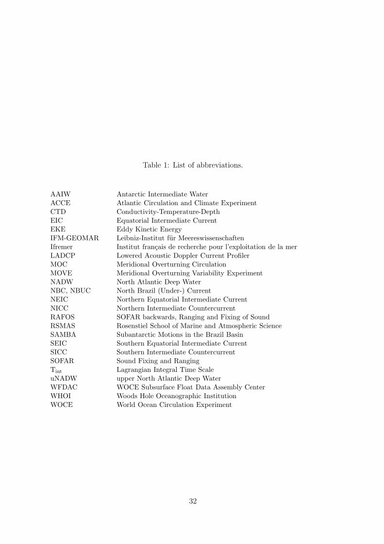
Table 1: List of abbreviations.

AAIW Antarctic Intermediate WaterACCE Atlantic Circulation and Climate ExperimentCTD Conductivity-Temperature-DepthEIC Equatorial Intermediate CurrentEKE Eddy Kinetic EnergyIFM-GEOMAR Leibniz-Institut fur MeereswissenschaftenIfremer Institut francais de recherche pour l’exploitation de la merLADCP Lowered Acoustic Doppler Current ProfilerMOC Meridional Overturning CirculationMOVE Meridional Overturning Variability ExperimentNADW North Atlantic Deep WaterNBC, NBUC North Brazil (Under-) CurrentNEIC Northern Equatorial Intermediate Current

NICC Northern Intermediate CountercurrentRAFOS SOFAR backwards, Ranging and Fixing of SoundRSMAS Rosenstiel School of Marine and Atmospheric ScienceSAMBA Subantarctic Motions in the Brazil BasinSEIC Southern Equatorial Intermediate CurrentSICC Southern Intermediate CountercurrentSOFAR Sound Fixing and RangingTint Lagrangian Integral Time ScaleuNADW upper North Atlantic Deep WaterWFDAC WOCE Subsurface Float Data Assembly CenterWHOI Woods Hole Oceanographic InstitutionWOCE World Ocean Circulation Experiment

32

Table 2: List of data used in this study. Note that some projects have collected more

data than is actually used here. WFDAC refers to the WOCE float data center at

wfdac.whoi.edu. Where individual persons are listed, the data was obtained directly

from them rather than through WFDAC. From SOFAR floats, only the first year of data

is used because of ballasting problems presumably worsening with age (Richardson and

Fratantoni, 1999). Argo drift pressures are based on nominal rather than measured values.

Project Float PrincipalData Source

Data Amount [d] Press. [dbar] Sampling

Name Type Investigators AAIW uNADW Mean ± Std. Period

MOVEAcoustic

(RAFOS)

U. Send,

W. Zenk

IFM-GEOMAR,

M. Lankhorst4370 2410

811 ± 30

1433 ± 125

2000–2001

2001–2001

NBCAcoustic

(RAFOS)

D. Fratantoni,

P. Richardson

WFDAC,

C. Wooding3030 0 861 ± 60 1998–2000

SAMBAAcoustic

(Marvor)

M. Ollitrault,

A. C. de Verdiere

Ifremer,

M. Ollitrault18953 0 813 ± 26 1994–2003

IFM

WOCE-era

Acoustic

(RAFOS)

O. Boebel,

W. Zenk

WFDAC,

M. Lankhorst930 0 833 ± 29 1994–1996

Trop. Atl.

SOFAR

Acoustic

(SOFAR)

P. Richardson,

W. SchmitzWFDAC 4610 3890

839 ± 72

1863 ± 39

1989–1990

1989–1990

Argo Profiling MultipleArgo Data

Centers37509 5975

1000 ± 50

1750 ± 250

1997–2006

2000–2006

ACCE

(WHOI)Profiling R. Schmitt

WFDAC,

E. Montgomery16351 99

981 ± 45

1247 ± 39

1997–2002

1998–2002

ACCE

(RSMAS)Profiling K. Leaman

WFDAC,

P. Vertes9659 3459

927 ± 114

1251 ± 38

1997–2002

1998–2002

33

Table 3: Mean transports in Sv for current features in the AAIW layer from different

studies in relation to this one. All values are adapted to a common layer thickness of

450 m.

MethodNBUC

at 8◦ SSEIC SICC EIC NICC NEIC

across

16◦ N

this study floats 5.0 2.7 4.1 3.2 4.5 3.2 3.7

Ollitrault et al. (2006) floats (800 dbar) – 4.7 5.4 3.9 5.8 2.5 –

Rhein et al. (2005) ring count, hydrography – – – – – – 2.9–4.5

Schott et al. (2003) ship LADCP 5.7 3.5 5.5 3.9 3.9 –

Boebel et al. (1999a) floats 4.5 – – – – – –

Schott et al. (1998) misc. shipborne 6.4–7.8 – 5.5 14.2 7.7 – –

34

60°W 50°W 40°W 30°W10°S

0°

10°N

20°N

Mooring

CTD / LADCP Station

Mid−Atlantic Ridge

Amazon

Caribbean Sea

B

T

CRAC

GPB

razi

l Bas

in

Guiana Basin

TB

BB

MOVE RAFOSNBC RAFOSSAMBA MARVORIFM WOCE−era RAFOSTrop. Atl. SOFARArgoACCE PALACE (WHOI)ACCE PALACE (RSMAS)

AAIW Floats:

60°W 50°W 40°W 30°W10°S

0°

10°N

20°N

EIC

SICC

NICC

NEIC

SEICNBUC

MOVE RAFOSTrop. Atl. SOFARArgoACCE PALACE (WHOI)ACCE PALACE (RSMAS)

uNADW Floats:

60°W 50°W 40°W 30°W10°S

0°

10°N

20°N

DWBC

Figure 1: Top: Map of the study area

indicating locations of two CTD sections

(cf. fig. 2) and various mooring locations

(cf. figs. 5 and 6). Abbreviations are:

AC Amazon Cone, B Barbados, BB Bar-

bados Basin, CR Ceara Ridge, GP Guiana

Plateau, T Trinidad, TB Tobago Basin.

Bathymetry in grey shades every 500 m

down to 4500 m with additional lines at

1000, 2000, and 3000 m.

Middle and bottom: Float data coverage

in the AAIW (middle panel) and uNADW

(bottom) layers. Colors indicate different

research projects. Each dot represents one

displacement of typically 10 d duration.

Schematics of major currents are included;

cf. table 1 for abbreviations.

35

Section 16°N

Dep

th [m

]

0 500 1000

0

500

1000

1500

2000

2500

Section 35°W

0 500 1000

0

500

1000

1500

2000

2500

DW

BC

Ring

Distance [km]

Dep

th [m

]

0 500 1000

0

500

1000

1500

2000

2500

NB

C

SIC

C

EIC

NIC

C

NE

IC

Distance [km]0 500 1000

0

500

1000

1500

2000

2500

Sal

inity

34.5

35

35.5

36

36.5

37

Vel

ocity

[cm

s−

1 ]

−20

0

20

60°W 55°W 50°W 5°S 0° 5°N

Figure 2: CTD and LADCP sections sampled during RV Sonne cruise 152 in late 2000

(Rhein et al., 2004, 2005). For locations of the two sections, cf. fig. 1: left-hand panels refer

to the section near 16◦ N, and right-hand panels to the one along 35◦ W. Top: Salinity

measurements from the CTD. Bottom: Across-section velocities from the LADCP (north-

and eastward positive), and matching geographic coordinates. Purple dots indicate station

locations, and the colored lines denote: depth of minimum salinity in the AAIW (white),

depth of local salinity maximum in the uNADW (blue), and isopycnals σ0 = 27.10,

σ1.5 = 34.42, and σ1.5 = 34.70 (green) representing AAIW and uNADW boundaries.

Labeled current features are discussed in the text (cf. table 1 for abbreviations).

36

65°W 60°W 55°W 50°W 45°W 40°W 35°W 30°W10°S

5°S

0°

5°N

10°N

15°N

20°N

EIC

SICC

NICC

NEIC

SEICNBUC

0

500

Map

Sca

le[k

m]

Streamline Spacing [km]

Spe

ed [c

m s

−1 ]

0 20 40 60 80 1000

10

20

30

Figure 3: Stream function derived from all float displacements in the AAIW layer. The

direction of flow is counterclockwise around reddish features and clockwise around blue

ones. Streamline spacing is 1000 m2s−1, yielding a volume transport of 0.1 Sv between

two streamlines for every 100 m of layer thickness. Cf. table 1 for abbreviations of named

currents. Bathymetry as in fig. 1.

37

65°W 60°W 55°W 50°W 45°W 40°W 35°W 30°W10°S

5°S

0°

5°N

10°N

15°N

20°N

5 15

cm s−1

Figure 4: Mean currents in the uNADW layer. Box shapes near the boundary follow

the flow features seen in individual trajectories (fig. 9). Arrow colors indicate scale.

Bathymetry in shades of grey every 500 m down to 4500 m.

38

Vel

ocity

[cm

s−

1 ]

(a)

0 200 400 600 800 1000

−20

−10

0

10

20

Vel

ocity

[cm

s−

1 ]

(b)

Distance [km]0 200 400 600 800 1000

−20

−10

0

10

20 (c)

NBUC NICC NEIC

Distance [km]0 200 400 600 800 1000

−20

−10

0

10

20

60°W 50°W 40°W 30°W10°S

0°

10°N

20°N

(a)

(b)

(c)

Figure 5: Velocities across three sections in the AAIW layer derived from float displace-

ments (red) and mooring records (green). Upper right: Map with the sections (black

lines), locations of data collection (red and green), and the stream function of fig. 3

(bluish, spaced every 2000 m2s−1) superimposed. Other panels: Light red dots refer to

individual float displacements of typically ten days duration. Red crosses average these

values in bins of 100 km; vertical extents of the crosses indicate 95% confidence intervals.

Mooring data are shown as green dots with 95% confidence limits. Mooring data are

from (a) the MOVE experiment, (b) Johns et al. (1990), and (c) Schott et al. (1993).

Abbreviations in (c) refer to named currents (cf. table 1).

39

Vel

ocity

[cm

s−

1 ]

(a)

0 200 400 600 800 1000

−40

−30

−20

−10

0

10

20

Vel

ocity

[cm

s−

1 ]

(b)

Distance [km]0 200 400 600 800 1000

−40

−30

−20

−10

0

10

20(c)

Distance [km]0 200 400 600 800 1000

−40

−30

−20

−10

0

10

20

60°W 50°W 40°W 30°W10°S

0°

10°N

20°N

(a)

(b)

(c)

Figure 6: Velocities across three sections in the uNADW layer (otherwise as fig. 5) derived

from float displacements (red) and mooring records (green). Mooring data are from (a)

the MOVE and GAGE (M. McCartney, pers. comm.) experiments, (b) from Johns et al.

(1990) and Colin et al. (1994), and (c) from Schott et al. (1993).

40

60°W 50°W 40°W 30°W10°S

0°

10°N

20°N

Data Amount [d]

0 200 400 600 800 1000

60°W 50°W 40°W 30°W10°S

0°

10°N

20°N

EKE [cm 2 s−2]

0 50 100 150 200

60°W 50°W 40°W 30°W10°S

0°

10°N

20°N

Tint

[d]

2 4 6 8 10

Figure 7: Lagrangian properties of the

eddy field in the AAIW layer derived from

float data with daily underwater position-

ing. Top: Data coverage in cumulative

float days. Middle: Lagrangian eddy ki-

netic energy (EKE). Bottom: Lagrangian

integral time scale (Tint). Bathymetric con-

tours are at every 1000 m down to 4000 m.

41

65°W 60°W 55°W 50°W

8°N

10°N

12°N

14°N

16°N

18°N

C

B

A

45°W 40°W 35°W 30°W5°S

0°

5°N

E

NEIC

NICC

EIC

SICC

SEIC

Figure 8: Eddy-resolving float trajectories of the AAIW layer. The selection is limited

to acoustic floats from the MOVE, NBC, and SAMBA projects for which tracking was of

good quality. Dots are at start points, arrow tips are 30 d apart. Single letters refer to

highlighted (red) trajectories discussed in the text (section 4.1), abbreviations to named

currents (cf. table 1). Bathymetry as in fig. 1.

42

60°W 50°W 40°W 30°W

0°

10°N

20°N

F

GH

JK

60°W 55°W 50°W8°N

10°N

12°N

14°N

16°N

18°N

F

G

H

J

K

Figure 9: Selected float trajectories of the uNADW layer. Trajectories are from three

profiling floats (ACCE RSMAS, shades of red) and the eddy-resolving acoustic MOVE

and SOFAR float projects (other colors). Arrows for the profiling floats show their ten-day

displacements, and arrow tips in the acoustic trajectories are 30 d apart. Letters refer to

trajectories discussed in the text (section 4.1). The bottom panel is a close-up of the box

marked in the top panel. Bathymetry as in fig. 1.

43

62°W 60°W 58°W10°N

11°N

12°N

13°N

14°N

15°N

Barbados

Trinidad

2001/8/23 −2001/9/22

Figure 10: Snapshot of three simultaneous float trajectories drifting at 1400 dbar in the

southward-flowing DWBC east of Barbados. The drift time was one month, yielding mean

currents of 14.6, 10.7, and 8.6 cm s−1 for the three trajectory segments. Bathymetry as

in fig. 1.

44

50°W 45°W 40°W0°

2°N

4°N

6°N

8°N

NEIC

45°W 40°W 35°W2°S

0°

2°N

4°N

6°N

NICC

45°W 40°W 35°W 30°W4°S

2°S

0°

2°N

4°N

EIC

40°W 35°W 30°W 25°W8°S

6°S

4°S

2°S

0°

SICC

40°W 35°W 30°W 25°W10°S

8°S

6°S

4°S

2°S

SEIC

60°W 50°W 40°W 30°W 20°W10°S

5°S

0°

5°N

10°N

all

NEIC NICC

EIC SICC SEIC

Figure 11: Interaction between the zonal equatorial currents and the boundary. Trajec-

tories that pass through the black boxes are displayed. Red shades represent trajectories

up to 80 d before entering the box, and green shades are trajectories up to 80 d after

leaving the box. Top left panel: All boxes and trajectories superimposed. Other pan-

els: Close-ups of individual boxes and corresponding trajectories. Boxes are designed to

represent the following currents (cf. fig. 3): NEIC, NICC, EIC, SICC, SEIC. Arrows in

the boxes indicate whether mean flow is generally east- or westward in the current band.

Bathymetry as in fig. 1, abbreviations as in table 1.

45

50°W 45°W 40°W 35°W 30°W5°S

0°

5°N

Figure 12: Crossing of the equator in the AAIW layer. Like in fig. 11, float trajectory

segments up to 80 d in duration before entering (red) and after leaving (green) the black

box are displayed. Trajectory segments in the box are included in white. Bathymetry as

in fig. 1.

46

60°W 50°W 40°W 30°W10°S

5°S

0°

5°N

10°N

15°N

20°N

AAIW

?

60°W 50°W 40°W 30°W10°S

5°S

0°

5°N

10°N

15°N

20°N

uNADW

?

Figure 13: Circulation schematics. Top: AAIW layer. Black arrows reproduce results by

Stramma and Schott (1999) and Schmid et al. (2003). Green arrows correct and extend

these. Red marks show where the previous results were disproven. Bottom: uNADW

layer. Black arrows interpret results by Richardson and Fratantoni (1999). Green arrows

show findings based on the present study.

47