July

The Measurement of Depreciation in theU.S. National Income and Product AccountsBy Barbara M. Fraumeni

As part of the recent comprehensive revision of the ’s, introduced an improved methodology for calculating de-preciation. The improved methodology uses empirical evidenceon the prices of used equipment and structures in resale mar-kets, which has shown that depreciation for most types of assetsapproximates a geometric pattern. Previously, the depreci-ation estimates were derived using straight-line depreciationand assumed patterns of retirements.

This article describes the theoretical and empirical litera-ture that supports the new methodology. The author,a professor of economics at Northeastern University, Boston,Massachusetts, drafted the article while she was serving as aconsultant to for this project. The views expressed are theauthor’s and do not necessarily represent those of .

T describes the basis for the newdepreciation methodology used by the Bu-

reau of Economic Analysis (). The new methodology reflects the results of empiricalstudies on the prices of used equipment andstructures in resale markets, which have shownthat depreciation for most kinds of equipmentand structures does not follow a straight-linepattern. For most assets, empirical studieson specific assets conclude a geometric patternof depreciation is appropriate. The new methodology also uses a geometric pattern ofdepreciation as the default option when informa-tion on specific assets is unavailable. In eithercase, the geometric (constant) rate of deprecia-tion is determined from empirical studies of usedassets. For some assets (autos, computers, mis-siles, and nuclear fuel), empirical studies, data, or technological factors justify the use ofa nongeometric pattern of depreciation by .This article reviews the empirical research on de-preciation, the basis for the improvement in methodology.

Previous estimates of depreciation werebased on a straight-line pattern for depreciation;the switch is to a geometric pattern for depre-

. The improved methodology was summarized in Parker and Triplett(). The new estimates of capital stock were described in Katz and Herman().

. These assets are listed as type A and B assets in table .

. These assets are listed as type C assets in table .

ciation for most assets. A straight-line patternassumes equal dollar depreciation over the life ofthe asset. For example, with straight-line depre-ciation, depreciation in the first year is equal todepreciation in the second year, which is equalto depreciation in the third year, and so on. Ageometric pattern is a specific type of acceleratedpattern. An accelerated pattern assumes higherdollar depreciation in the early years of an asset’sservice life than in the later years. For exam-ple, with accelerated depreciation, depreciationin the first year is greater than that in the sec-ond year, which is in turn greater than that inthe third year, and so on. In calculations,in the absence of investment, geometric deprecia-tion is calculated as a constant fraction of detailedconstant-dollar net stocks.

In most cases, the rates of geometric depreci-ation are based on the Hulten-Wykoff estimates(Hulten and Wykoff b). For some assets(computer equipment and autos), nongeometricdepreciation rates estimated in empirical studiesor from data are used. For a few as-sets (missiles and nuclear fuel rods), hasretained its prior methodology of deriving esti-mates of depreciation using straight-line depre-ciation and Winfrey retirement patterns. Theoriginal Hulten-Wykoff rates are modified toreflect service lives currently used by .

The first section of this article briefly describesthe relevant depreciation concepts. The secondsection discusses previous methodology andHulten-Wykoff methodology in the context ofthese depreciation concepts. The empirical re-search on depreciation is summarized in the thirdsection. In the fourth section, the new depreciation rates for all assets except autos, com-puters, missiles, and nuclear fuel are listed andtheir derivation documented. The fifth sectionconsists of a brief conclusion.

. Retirement patterns refer to the patterns of assets withdrawn fromservice.

• July

Tab

Represent the price

A change in the pr

de

re

Schematically, repr(Ptime=,age= − Ptime=changes over time = 0R is revaluation:

Ptime=,age=

↓D↓

AGE Ptime=,age=

.

.

.

Ptime=,age=

Depreciation Concepts

Definitions

The value of an asset changes as the result of de-preciation and revaluation. Depreciation is thechange in value associated with the aging of anasset. As an asset ages, its price changes becauseit declines in efficiency, or yields fewer productiveservices, in the current period and in all futureperiods. Depreciation reflects the present value ofall such current and future changes in productiveservices.

Revaluation is the change in value or price perunit that is associated with everything other thanaging. Revaluation includes pure inflation, obso-lescence, and any other impact on the price of anasset not associated with aging.

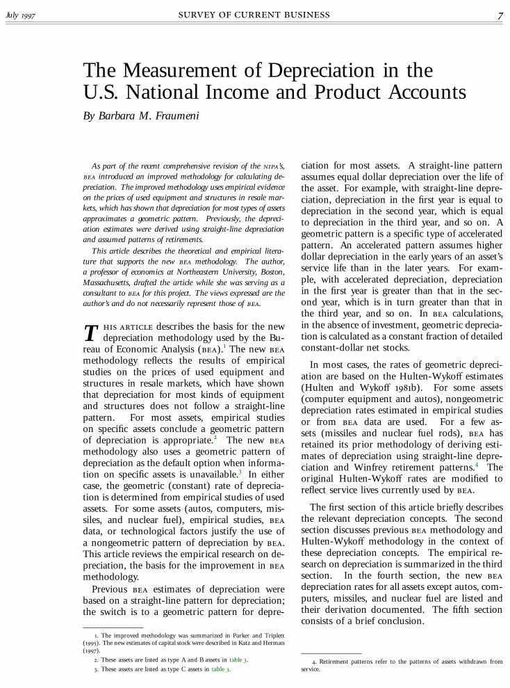
The decomposition of the change in the valueof an asset is illustrated in table for an asset withprice per unit. The price of an asset, Ptime,age ,in time and the price of an asset in time isobserved. There are two possible sources of theprice change: The first being a change in the priceof an asset because it has aged and the second

. The sources for this section include papers by Triplett (a, b,), by Jorgenson (, ), by Young and Musgrave (), and by ().

. and the author of this article differ in their definition of depreci-ation in national accounts. This will be discussed briefly in the section “definition.”

le 1.—Depreciation Versus Revaluation

of an asset by (Ptime,age).

ice of an asset at time = 1, (Ptime=,age= − Ptime=,age=),is equal to

preciation, (Ptime=,age= − Ptime=,age=),or age effects, holding time constant

plusvaluation, (Ptime=,age= − Ptime=,age=),or time effects, holding age constant.

esenting the decomposition of the observed price change,age=), in bold and with arrows, and the matrix of price,1, . . . T and age = 0,1, . . . A, where D is depreciation and

TIME

Ptime=,age= Ptime=,age= . . . Ptime=T,age=

����↘→ R→ Ptime=,age= Ptime=,age= . . . Ptime=T,age=

. . . . . .

. . . . . .

. . . . . .

A Ptime=,age=A Ptime=,age=A . . . Ptime=T,age=A

being a change in the price of an asset because itis a different time period. The decomposition canbe illustrated in the simplest case by reference tothe well-known used-car price book. Prices for -year-old cars of the same make and model in the book and their prices when new provide anestimate of depreciation because everything butage is held constant. Prices for -year-old cars ofthe same make and model in the and price books provide an estimate of revaluation,because age is held constant while everything elsechanges.

Obsolescence is a decrease in the value of anasset because a new asset is more productive, ef-ficient, or suitable for production. A new assetmight be more suited for production because iteconomizes on an input that has become rela-tively more expensive. Obsolescence has played abig part in the debate about the impact of the oilembargo on productivity. Other impacts on theprice of an asset include the price effect of anychanges in taxes or interest rates facing businessnot anticipated when the asset was new. If depre-ciation and retirement patterns did not changeover time, revaluation could be estimated from aused-asset-price book, as described above.

definition

defines depreciation as “the decline in valuedue to wear and tear, obsolescence, accidentaldamage, and aging” (Katz and Herman ,), which includes retirements, or discards asthey are frequently called. includes the de-struction of privately owned fixed assets that isassociated with natural disasters in depreciation.

focuses on depreciation as the consumptionof fixed capital or as a cost of production. De-preciation is viewed as a cost incurred in theproduction of gross domestic product (), as adeduction in the calculation of business income,

. Martin N. Baily () argues that the rapid increase in energy pricesduring the oil embargo rendered certain types of assets obsolete, leading toa decline in the rate of productivity change. A rebuttal to this argument iscontained in Hulten, Robertson, and Wykoff ().

. Retirements or discards are assets withdrawn from service.

. The current treatment of natural disasters in part reflects theabsence from the national income and product accounts of an integratedbalance sheet and raises another set of issues that will not be discussed here.

The author wishes to thank Ernst Berndt, Eric Brynjols-son, Terry Burnham, Madeline Feltus, Michael Harper,Charles Hulten, Dale Jorgenson, Peter Koumanakos,Stephen Oliner, Keith Shriver, Kevin Stiroh, and FrankWykoff, as well as staff at , for their comments andassistance on this article.

July •

and as a partial measure of the value of servicesof government fixed assets. ’s conceptualiza-tion of depreciation as such is generally consistentwith the work of Fabricant (, –) andDenison () and the definition of depreciationin the System of National Accounts (). It isalso consistent with the concept of the consump-tion of fixed capital in the context of estimatesof sustainable product, or income, where de-preciation is subtracted from to derive netdomestic product and net domestic income—arough measure of that level of income or con-sumption that can be maintained while leavingcapital intact.

The essential difference between ’s depreci-ation definition and the definition in this articleis the treatment of obsolescence. Obsolescenceshows up in the national income and productaccounts (’s) in at least two ways. One, depreciation estimates include obsolescencethrough a service-life effect and through the useof depreciation rates estimated from used-assetprices unadjusted for the effects of obsolescence.Assets may be retired early, when they are stillproductive, because of obsolescence; this is re-flected in ’s depreciation estimates, as servicelives affect the estimate of the geometric rates ofdepreciation used for most assets. Two, obso-lescence is reflected in the constant-quality pricesthat are part of the ’s. In addition to thetheoretical usefulness of separating the effects ofobsolescence from those associated with the phys-ical deterioration of an asset, ’s use of hedonicand other quality-adjusted price indexes suggestsan empirical reason why greater attention mayhave to be paid to the effects of obsolescence.In its future work, plans to conduct studiesfocusing on quality change and obsolescence.

. The defines depreciation as “the decline, during the course of theaccounting period, in the current value of the stock of fixed assets owned andused by a producer as a result of physical deterioration, normal obsolescence,or normal accidental damage” ( , , .).

. See the next section and “ default geometric-depreciation rates.”

. See Oliner (, ) for a discussion of constant-quality prices anddepreciation in the context of a study of mainframe computers. is usingOliner’s partial depreciation measure, which is consistent with ’s hedonicprice index for computers.

. The author of this article and both agree that further work needsto be done to quantify obsolescence and to identify the impact of obsoles-cence and quality change on national income accounting measures. Furtherconsideration of the major issues surrounding the definitional differences de-scribed above could be one component of future work on obsolescence andquality change.

Specifics of Methodology andHulten-Wykoff Methodology

Specifics of methodology

As noted, has used a straight-line pattern ofdepreciation since the ’s. Depreciation is anequal dollar amount per period over the lifetimeof the asset.

Retirements for a group of assets depended onthe group’s average service life and on the patternof retirements (the distribution of retirementsaround the mean service life).

Once retirements have begun, the combinedeffects of straight-line depreciation and retire-ments result in a depreciation pattern that ismore accelerated than a straight-line deprecia-tion pattern. An accelerated depreciation patternassumes higher dollar depreciation in the earlyyears of an asset’s service life than in the lateryears.

Mean service lives are estimated from a widevariety of sources, both government and pri-vate. In general, information is not available toprovide different mean service lives by industry.Production-type manufacturing equipment is anotable exception. Similarly, in general, informa-tion is not available on changes in mean servicelives over time, if they do occur; aircraft is oneexception to this general rule. When a meanservice life is changed, the new mean service lifeis applied only to new assets. There is no effecton depreciation of existing assets.

A modified S- Winfrey curve was used formost assets to estimate the pattern of actual re-tirements around the mean; a L- Winfrey curvewas used for consumer durables (Winfrey ;Russo and Cowles ). The S- curve is a bell-shaped distribution centered on the mean servicelife of the asset. It was used for private nonresi-dential equipment (except autos) and structures,private residential equipment, and governmentresidential equipment and structures. The L-curve is an asymmetrical distribution with heav-ier discards before the mean service life. Both setsof Winfrey curves were modified to reflect differ-ent assumptions about when retirements beginand end as a percentage of the mean service lifeof the asset.

Expected obsolescence implicitly enters into estimates of depreciation through shorter as-set lifetimes and through the retirement patternpreviously used. The mean service life of a classof assets could be shorter because obsolescence

. See ().

• July

. The censored-sample problem can be illustrated by the following ex-ample. Suppose that two cars are bought new in . By , one is still

has occurred consistently over the historical pe-riod or is reflected in the occasional revision ofmean service lives. In addition, as obsolescencecan result in early retirement, the modified Win-frey patterns may have been picking up some ofthe obsolescence effects.

adjusts depreciation estimates to capturethe effect of natural disasters that destroy largeamounts of fixed capital.

Specifics of Hulten-Wykoff methodology

Initially, Hulten and Wykoff made no assumptionabout what form depreciation patterns take. In-stead, they estimated used-asset age-price profilesfor eight producers’ durable equipment or non-residential equipment assets, which they calledtype A assets, with a Box-Cox model (Boxand Cox ). They tested to see whetherthe resulting depreciation patterns most nearlyresembled patterns arising from one-hoss-shay,straight-line, or geometric efficiency patterns.

There is a direct correspondence betweenefficiency patterns and depreciation patterns.Present and future declines in efficiency result indepreciation or declines in the value of an as-set as it ages. A one-hoss-shay efficiency patternassumes that no loss in efficiency occurs untilthe asset is retired. The corresponding deprecia-tion pattern is less accelerated than a straight-linepattern of depreciation with lower dollar depre-ciation in the early years of an asset’s service lifethan in the later years. A straight-line efficiencypattern assumes equal declines in efficiency ineach period over the life of the asset. The corre-sponding depreciation pattern, which has higherdollar depreciation in the early years of an asset’sservice life than in the later years, is acceleratedrelative to a straight-line pattern of depreciation.A geometric efficiency pattern also gives rise to anaccelerated depreciation pattern. The geometricpattern is a special case because the efficiency pat-tern and the depreciation pattern have the sameform, with declines in efficiency and depreciationoccurring at the same rate.

Hulten and Wykoff concluded that depreci-ation patterns for eight assets are accelerated.In addition, although all three patterns were

. Young and Musgrave maintain that expected obsolescence should becharged when the asset is retired (Young and Musgrave , , figure .).’s methodology does not do this.

. The information on Hulten-Wykoff methodology is taken from threesources: Hulten and Wykoff (a and b) and Wykoff and Hulten ().

. Age-price profiles map ages of assets with their prices.

. An efficiency pattern is a pattern describing the productive servicesfrom an asset as it ages. The efficiency of a new asset is typically normalizedto .. As an asset declines in efficiency, its efficiency has a value of less thanone.

rejected statistically, they concluded that thedepreciation pattern was approximately geomet-ric in all cases. In , the eight producers’durable equipment or nonresidential equipmentassets—tractors, construction machinery, met-alworking machinery, general industrial equip-ment, trucks, autos, industrial buildings, andcommercial buildings—amounted to percentof investment expenditures on producers’ durableequipment and percent of spending on non-residential structures. They assumed that the de-preciation pattern for the remaining out of producers’ durable equipment and nonresiden-tial structures classes contemporary to theirstudy was geometric. These were categorized astype B or type C assets.

Since used-asset prices reflect only surviv-ing assets (a censored-sample problem), Hultenand Wykoff weighted used-asset prices by theprobability of survival before estimating the de-preciation patterns. Weighted used-asset pricesreflect surviving and retired assets. The proba-bility of survival, the weight, depends upon themean service lives of assets and on the devia-tion of retirements around the mean service life.Mean service lives were assumed to be per-cent of Bulletin F. An L0 Winfrey curve wasused to estimate the pattern of actual retirementsabout the mean for structures. The L0 curveis an asymmetrical distribution that allows forsome assets to survive to very old ages relative tothe mean service lives. An S- curve, describedabove, was used for metalworking machinery andgeneral industrial machinery. Finally, an as-sumption was needed about the net value of anasset (scrappage value less demolition costs) tocomplete the transformation of a surviving-assetsample to an estimated sample of both survivingand retired assets. Hulten and Wykoff assumedthat the net value of an asset retired from servicewas on average zero. The used-asset prices in-putted to the Box-Cox model were thus weightedand net value adjusted. As a result, the deprecia-tion estimates from the Box-Cox model reflectedboth efficiency declines and retirements.

in service and one has been junked. The one that is still is service is soldas a used car, say for ,. If we take the used-car sales price to be rep-resentative of all cars bought new in , we would assume that the value of all cars bought new in is ,. In fact, the value of thecars is , or on average per car. Hulten and Wykoff, by weightingused-asset prices by the probability of survival, are calculating the used-assetprice equivalent of an average value of per car bought new in .Their procedure assumes that the used-asset price of nonsurvivors is zero.

. at the time typically assumed mean service lives were percentof Bulletin F and used a modified S- Winfrey curve for most assets exceptconsumer durables.

July •

. With truncation, . was frequently used in the actual calculations.

. At the time of Hulten and Wykoff’s research, researchers commonlyassumed that the appropriate declining-balance rate was double declining.

. This section draws heavily on three previous surveys of empirical re-search on depreciation. They are Hulten and Wykoff (b), Jorgenson(), and Brazell, Dworin, and Walsh ().

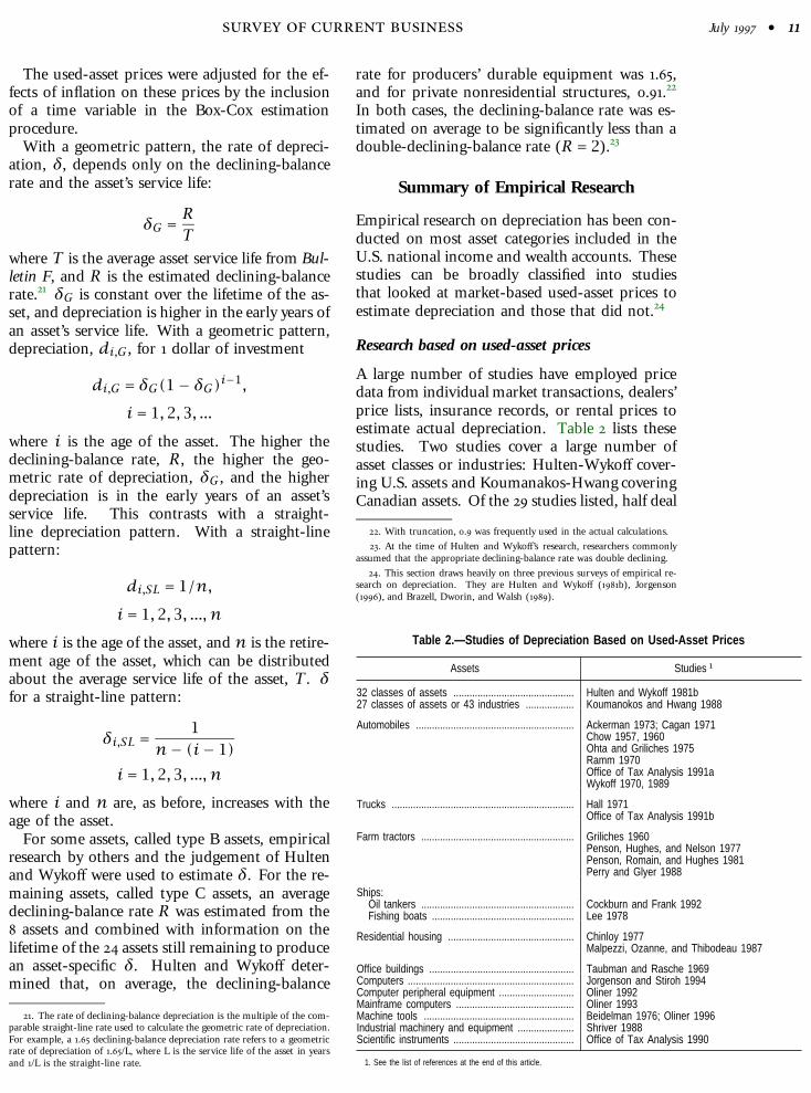
Table 2.—Studies of Depreciation Based on Used-Asset Prices

Assets Studies 1

32 classes of assets ............................................. Hulten and Wykoff 1981b27 classes of assets or 43 industries .................. Koumanokos and Hwang 1988

Automobiles ........................................................... Ackerman 1973; Cagan 1971Chow 1957, 1960Ohta and Griliches 1975Ramm 1970Office of Tax Analysis 1991aWykoff 1970, 1989

Trucks .................................................................... Hall 1971Office of Tax Analysis 1991b

Farm tractors ......................................................... Griliches 1960Penson, Hughes, and Nelson 1977Penson, Romain, and Hughes 1981Perry and Glyer 1988

Ships:Oil tankers ......................................................... Cockburn and Frank 1992Fishing boats ..................................................... Lee 1978

Residential housing ............................................... Chinloy 1977Malpezzi, Ozanne, and Thibodeau 1987

Office buildings ...................................................... Taubman and Rasche 1969Computers .............................................................. Jorgenson and Stiroh 1994Computer peripheral equipment ............................ Oliner 1992

The used-asset prices were adjusted for the ef-fects of inflation on these prices by the inclusionof a time variable in the Box-Cox estimationprocedure.

With a geometric pattern, the rate of depreci-ation, δ, depends only on the declining-balancerate and the asset’s service life:

δG =RT

where T is the average asset service life from Bul-letin F, and R is the estimated declining-balancerate. δG is constant over the lifetime of the as-set, and depreciation is higher in the early years ofan asset’s service life. With a geometric pattern,depreciation, di,G , for dollar of investment

di,G = δG(1− δG)i−1,

i = 1,2,3, ...

where i is the age of the asset. The higher thedeclining-balance rate, R, the higher the geo-metric rate of depreciation, δG , and the higherdepreciation is in the early years of an asset’sservice life. This contrasts with a straight-line depreciation pattern. With a straight-linepattern:

di,SL = 1/n,

i = 1,2,3, ..., n

where i is the age of the asset, and n is the retire-ment age of the asset, which can be distributedabout the average service life of the asset, T . δfor a straight-line pattern:

δi,SL =1

n− (i− 1)i = 1,2,3, ..., n

where i and n are, as before, increases with theage of the asset.

For some assets, called type B assets, empiricalresearch by others and the judgement of Hultenand Wykoff were used to estimate δ. For the re-maining assets, called type C assets, an averagedeclining-balance rate R was estimated from the assets and combined with information on thelifetime of the assets still remaining to producean asset-specific δ. Hulten and Wykoff deter-mined that, on average, the declining-balance

. The rate of declining-balance depreciation is the multiple of the com-parable straight-line rate used to calculate the geometric rate of depreciation.For example, a . declining-balance depreciation rate refers to a geometricrate of depreciation of ./L, where L is the service life of the asset in yearsand /L is the straight-line rate.

rate for producers’ durable equipment was .,and for private nonresidential structures, ..

In both cases, the declining-balance rate was es-timated on average to be significantly less than adouble-declining-balance rate (R = 2).

Summary of Empirical Research

Empirical research on depreciation has been con-ducted on most asset categories included in theU.S. national income and wealth accounts. Thesestudies can be broadly classified into studiesthat looked at market-based used-asset prices toestimate depreciation and those that did not.

Research based on used-asset prices

A large number of studies have employed pricedata from individual market transactions, dealers’price lists, insurance records, or rental prices toestimate actual depreciation. Table lists thesestudies. Two studies cover a large number ofasset classes or industries: Hulten-Wykoff cover-ing U.S. assets and Koumanakos-Hwang coveringCanadian assets. Of the studies listed, half deal

Mainframe computers ............................................ Oliner 1993Machine tools ........................................................ Beidelman 1976; Oliner 1996Industrial machinery and equipment ..................... Shriver 1988Scientific instruments ............................................. Office of Tax Analysis 1990

1. See the list of references at the end of this article.

• July

with mechanized vehicles (automobiles, trucks,or farm tractors). Data on used prices are read-ily available for these assets. Three studies eachinvestigate depreciation for computers and realestate. Two studies each cover ships (fishingboats and oil tankers) and machine tools. Onestudy, by Shriver, deals with industrial machin-ery and equipment. The remaining study is astudy of scientific instruments by the Office ofTax Analysis. A variety of methodological ap-proaches were used. They include hedonics, ananalysis of variance, and Box-Cox or polynomialforms for the estimated equation.

General issues affecting used-asset-price studies

All used-asset-price studies are potentially biased,because the asset sample may not be represen-tative of the population as a whole or becauseeconomic conditions affect prices. First, assetsamples normally represent only surviving as-sets. Second, surviving-asset samples or theirsale prices may not represent the population ofsurviving assets. Third, changes in economicconditions, including taxes and interest rates,may affect used-asset prices. Finally, a used-assetprice may be affected by the value of an associatedinput.

If asset samples represent only surviving as-sets, then age-price profiles of used-asset samplesunderestimate depreciation for the population asa whole because retirements are not included.

Hulten and Wykoff estimated for commercial andindustrial buildings that such an error wouldreduce depreciation estimates by more than one-half. There are two possible solutions to thisproblem. One, retirements can be added to de-preciation, similar to the way modifies itsstraight-line depreciation pattern to allow for thepattern of retirements. Two, a censored-sampleadjustment can be made to the used-asset pricesbefore the depreciation pattern is estimated, ina manner similar to Hulten and Wykoff. Itis important for the researcher and user toknow whether the depreciation pattern includesretirements (as in Hulten-Wykoff) or excludesretirements (as in the accounts). A straight-line pattern excluding retirements will no longerbe a straight-line pattern once retirements are

. Triplett (, ) defines a hedonic function as a relation betweenprices of varieties or models of heterogeneous goods—or services—and thequantities of characteristics contained in them. A Box-Cox model is a modelthat transforms the form of the variables in the model (Box and Cox ).

. The authors who have addressed the question of sample bias inused-asset-price studies include Triplett (), DeLeeuw (), Hulten andWykoff (b) and Boskin, Robinson, and Roberts ().

. An example illustrating this point is given in footnote .

included, and a geometric pattern excluding re-tirements will no longer be a geometric patternonce retirements are included.

Surviving-asset samples or their prices maynot represent the population of surviving assets.Business may put up for sale their superior orinferior assets. Assets may be worth more or lessto the buyers than to the sellers. Finally, buyersmay not be able to accurately perceive the valueof the assets for sale.

It is not clear what is the extent or direction ofa possible surviving-asset-sample bias. Whetheror not businesses put up for sale their superior orinferior assets depends on whether they are try-ing to maximize the proceeds from such sales orto sell off less desirable or obsolete assets. Differ-ences in buyer-versus-seller asset value may biasused-asset prices in either direction as well. Adeclining business may be selling off an asset thatrepresents idle capacity and that another businessin the same industry could fully utilize or an assetthat has limited use to businesses in other indus-tries. Assets may be configured to meet the needsof a particular business so that they are morevaluable to their seller than to their buyer. Fi-nally, buyers may underestimate or overestimatethe value of used assets for sale.

The lemons hypothesis maintains that the valueof assets for sale will underestimate the value ofall assets in the stock (Ackerlof ). It arguesthat a disproportionate number of assets sold willbe lemons, particularly if inspection by buyersdoes not reveal which assets are lemons. Underthe lemons hypothesis, buyers will assume thatassets for sale are lemons; therefore, they will of-fer lower prices for all used assets. Sellers havean incentive to offer lemons, since they will bepaid lemons prices for both lemons and moredesirable assets. Therefore, buyers’ assumptionsare validated. If sellers have superior assets forsale, the incentive will be to sell these privatelyto obtain a reasonable price for the asset. Used-asset prices will be less than the average price ofthe stock of assets because of the disproportion-ate number of lemons for sale and because buyerswill assume all used assets are lemons. The exis-tence of asymmetric information between buyerand seller is crucial in this hypothesis. Depre-ciation would be overestimated if inferred fromused-asset prices because the average price forassets in the stock would be underestimated.

Hulten and Wykoff argue that most assets aresold in markets with professional buyers who fre-quently buy and sell assets. Furthermore, thesebuyers, who have the knowledge and expertise

July •

to identify lemons, are not affected by asymmet-ric information. Hulten and Wykoff tested forthe existence of a lemons bias by comparing thedepreciation profiles of assets that might havea lemons bias to an asset that arguably wouldnot (heavy construction equipment). Heavy con-struction equipment is commonly sold at the endof a construction project and repurchased at thebeginning of the next construction project. Theyfound that the depreciation profiles for assetspossibly with and without a lemons bias wereboth approximately geometric; therefore, theyconcluded that the lemons bias is unimportantin depreciation estimates.

Changes in tax laws, interest rates, and othereconomic conditions might affect the value ofsecondhand assets independently of any sam-ple bias problems. For example, changes inallowable tax depreciation taken for corporate in-come tax purposes may change the prices thatbusinesses are willing to pay for used assets.Changes in interest rates may affect the cost ofborrowing to finance asset acquisition. Finally,demand conditions determine whether businessesare expanding or contracting, affecting both thedemand for and supply of used assets. Obso-lescence can also affect used-asset prices, as, forexample, discussed above in the context of theenergy crisis.

If changes in tax laws, interest rates, and othereconomic conditions significantly affect the valueof secondhand assets, age-price profile or retire-ment patterns would change over time unlessthese changes are counterbalanced by offsettingeffects. The question of whether the age-priceprofile or retirement patterns change over timehas been discussed in the context of several em-pirical studies. Hulten and Wykoff (a, b)tested the stability of the age-price profiles foroffice buildings, one of their largest samples. Inalmost all cases, estimates of the rate of depreci-ation were stable over time. Hulten, Robertson,Wykoff, and Shriver reached similar conclusions.Hulten, Robertson, and Wykoff () lookedat the effect of the energy crisis on used-assetprices for four types of used machine tools andfive types of construction equipment. Shriver(b) looked at the rates of economic depre-ciation for industrial machinery and equipmentin different years with different demand char-acteristics. Cockburn and Frank () found ina study of oil tankers that economic deprecia-tion or decay was largely unaffected by economicconditions, but that retirements are quite sen-

. For example, see footnote .

sitive to economic conditions. Powers (),using book values, found that retirements fortwo-digit Standard Industrial Classification man-ufacturing industries exhibit a cyclical pattern.Taubman and Rasche () and Feldstein andRothschild () discuss in general the impactof variables that change over time on age-priceprofiles. Taubman and Rasche () in theirstudy of office buildings found that changes inrents and tax laws had little effect on deprecia-tion rates. In most cases, studies have not beendone on different vintages of assets to determinewhether age-price profiles do significantly changeover time. Therefore, there is no definitive an-swer to the question of whether age-price profilesshift over time.

In addition, used-asset prices can reflect thefact that it may be difficult for buyers to separatethe value of an asset such as a building from thevalue of the land on which it sits (the shopping-mall effect). The building may be incorrectlyvalued because of the value of the site or the landon which it sits.

Summary of research based on used-asset prices

Most of the used-asset studies do not directlydeal with possible biases arising from sam-ples, such as those discussed in the previoussection (see table ). In any case, the ex-tent and the net direction of the possible bi-ases are unclear. Four studies—Hulten-Wykoff,Koumanakos-Hwang, Oliner (), and Perry-Glyer—did adjust used-asset prices downward toreflect zero valuation of retired assets in the orig-inal cohort. In addition, the Cockburn-Frankpaper illustrates how misleading it can be to esti-mate patterns of depreciation without accountingfor retirements.

Of the two studies covering a large number ofasset classes or industries, Hulten and Wykoff’shas already been discussed. The Koumanakos-Hwang study of Canadian assets, the other study,bears a number of similarities to the Hulten-Wykoff study. It used a modified Box-Cox modelto estimate depreciation for up to differentasset classes for manufacturing and nonmanu-facturing separately. Depreciation for buildingconstruction and machinery and equipment forup to different industries were calculated froma weighted average of the depreciation functionsof individual assets. Some depreciation estimateswere done for engineering construction as well.Koumanakos and Hwang conclude that depreci-ation patterns for individual assets are approx-imately geometric for both the manufacturing

• July

and nonmanufacturing sectors, with the degreeof convexity more pronounced in the manu-facturing sectors. At the industry level, theyconclude that the geometric pattern is preferredbecause it is the simplest pattern that gives a bestapproximation of the actual data.

The papers on motorized vehicles (automo-biles, pickup trucks, or farm tractors) can be dis-tinguished by whether a depreciation pattern wasassumed, whether the validity of such assump-tions were tested econometrically, and whetherany general statements were made about the pat-tern of the used asset-price profile observed orestimated.

Ackerman () and Cagan () for auto-mobiles and Griliches () for farm tractorsassumed a geometric rate of depreciation, and inthe case of Ackerman and Cagan, the assumptionallowed for the separate identification of quality.None of these models were tested to see if theassumption of a geometric rate was appropriate.

Seven studies—one for trucks (Hall ), threefor automobiles (Ohta and Griliches ; Wykoff, ), and three for farm tractors (Pen-son, Hughes, and Nelson ; Penson, Romain,and Hughes ; Perry and Glyer )—testedthe appropriateness of a geometric assumption.With the exception of the two studies by Pen-son and others and one by Perry-Glyer, thesestudies concluded that although the assumptionof a geometric rate was not proven, that a ge-ometric rate, in the words of Hall (, ),“is probably a reasonable approximation for mostpurposes.” Perry and Glyer found in their econo-metric model, which excluded tractor care andusage, that depreciation rates were constant overtime. However, they found that depreciationrates were not constant when these variableswere omitted. In their two studies, Penson andothers estimated from engineering data that thepattern of productive-capacity depreciation forfarm tractors lies in between straight-line andone-hoss-shay. However, if productive-capacitydepreciation is one-hoss-shay, depreciation asdefined in this article follows a concave, orbowed-away-from-the-origin, pattern. Someresearchers found that the first-year decline inasset prices was significantly greater than the de-

. A convex depreciation pattern is bowed towards the origin in a graphof price versus age.

. Productive-capacity depreciation is measured by the additions to pro-ductive capacity required to maintain productive capacity at a constant level.If an asset does not decline in efficiency or productive services yielded overits lifetime until it is retired, (the lightbulb example), depreciation as definedin this article still occurs because as the asset ages, it is getting closer to itsretirement (or light-going-out) date. The present value of future declines inefficiency increases or depreciation occurs even if there is no current declinein efficiency.

cline suggested by a geometric rate (Wykoff ;Ackerman ), but question whether listedprices accurately represent transactions prices.Ohta and Griliches (, ), though conclud-ing that a geometric assumption is “not toobad an assumption ‘on the average’,” concludewithout empirically testing that actual deprecia-tion occurs at a faster rate with age. There isevidence among the other studies that geomet-ric rates may change over time (Ackerman ;Perry and Glyer ; Wykoff ), but there isno conclusive econometric evidence or consen-sus about the direction of the change. None ofthe motorized-vehicle studies performed econo-metric tests for the existence of other than ageometric depreciation pattern.

Three studies—one for trucks ( b)and two for automobiles ( a; Ramm)—calculated or econometrically estimatedused-asset age-price profiles, but did not reportany attempts to determine the general shape ofthe depreciation pattern. However in each study,in general the age-price profile initially declinedmore rapidly than it would under a straight-linepattern of depreciation.

Lee () and Cockburn and Frank ()studied ships. The Lee study looked at data onthe insured value of Japanese fishing boats as aproxy for new- and used-asset prices. The es-timated depreciation pattern was geometric insome cases (in general for steel boats) and not inothers (in general for wooden boats). Cockburnand Frank concluded that a geometric patternis an appropriate pattern for surviving-asset age-price profiles, but with proper accounting forretirements as a component of economic depre-ciation, the pattern of economic depreciation isclearly not geometric. Neither study consideredor tested for other commonly used depreci-ation patterns, such as patterns arising fromstraight-line or one-hoss-shay efficiency patterns.

Beidleman () and Oliner () estimateddepreciation for machine tools or assets sold bymachine-tool builders. Beidleman’s study of salesby machine-tool builders, which are primarilymachine tools, concluded that a negative expo-nential function was best able to explain asset-value variation in the majority of cases. Thissupports the assumption of a geometric depreci-ation pattern. Beidleman tested linear, exponen-tial, reciprocal, polynomial, and parabolic func-tions as possible alternatives. Oliner concludedthat when used-machine-tool prices are adjusted

. A negative exponential function estimates a geometric rate ofdepreciation.

July •

for retirements, the pattern of depreciation isnot geometric. However, based on the evidencefrom machine tools, actual depreciation for met-alworking machinery is more rapid during theearly years and the pattern more accelerated than formerly had assumed.

Two studies—Chinloy () and Malpezzi,Ozanne, and Thibodeau ()—looked at resi-dential real estate and one study—Taubman andRasche ()—looked at commercial real estate.The Chinloy study of sale prices for residentialreal estate concluded that the hypothesis of ageometric rate of depreciation could not be re-jected. The Malpezzi-Ozanne-Thibodeau studyon the other hand concluded that the decline inthe value of owner-occupied housing with ageoccurs at an increasing, not a constant, rate butthat rents for residential real estate decline withage of the property at a nearly constant or geo-metric rate. The Taubman-Rasche study of officebuildings, in contrast to most other studies ofdepreciation, concluded that depreciation occursat a rate slower than straight-line and, in fact,that a depreciation pattern arising from a one-hoss-shay efficiency pattern is a more appropriatepattern. This result may be due to the exis-tence of relatively long-term, fixed-price leases foroffice buildings.

Three studies measure depreciation of com-puters or computer peripheral equipment—twoby Oliner (, ) and one by Jorgensonand Stiroh (). All three studies assumethat the efficiency of assets in this category isconstant over time or best described by a one-hoss-shay pattern, but Oliner includes a measureof partial depreciation. Oliner defines partial de-preciation as the effect of age on price that isnot captured by a hedonic equation and that isunmeasured, because researchers are unable toidentify all relevant characteristics. The patternof partial depreciation appears to be approxi-mately geometric for all the computer peripheralequipment studied, except for disk drives. Thepattern of partial depreciation for mainframecomputers was decidedly not geometric, becausethe values of mainframes did not always con-sistently decline with age. The issue of theappropriate measure of depreciation for comput-ers will be discussed in the section “The New Depreciation Estimates.”

Shriver’s study of machinery and equipment() concluded that used-asset values decline

. Leases are payments for office building services, most likely reflectingproductive capacity (see footnote ), not the present value of future (post-lease) declines in efficiency.

at a rate that is faster than straight-line depre-ciation but slower than double-declining-balancedepreciation.

The Office of Tax Analysis study of scientificinstruments () did not report any attempts todetermine the general shape of the depreciationpattern. However, the age-value profile appearsto approximate a geometric pattern, even afteradjusting for retirements.

Other research

The major approaches used in nonprice-basedresearch on depreciation include a retirement ap-proach, an investment approach, a polynomialbenchmark approach, and a factor-demand, orproduction-model, approach. In addition, thereare a number of studies whose primary empha-sis is on the estimation of retirement patterns oruseful lives.

With a retirement approach, retirements areestimated. These retirements are then appliedto an assumed depreciation pattern to derivean estimate of actual depreciation. Former methodology is an example of such an ap-proach, modified with adjustments to reflectnatural disasters. Retirements depended uponservice lives and the assumed Winfrey distribu-tion of retirements around the mean retirementage. The pattern of depreciation was assumed tobe straight-line.

With an investment approach, an investmentmodel is used to estimate depreciation or thepattern of depreciation. Robert Coen (,) used a neoclassical investment model todetermine which of possible loss-of-efficiencypatterns—one-hoss-shay, straight-line, geomet-ric, or sum-of-the-years’-digits—best explainedinvestment flows into manufacturing indus-tries. A one-hoss-shay loss-of-efficiency patterntranslates into a depreciation pattern that is lessaccelerated than straight-line; the other three pat-terns translate into depreciation patterns that areconvex, or bowed towards the origin. For equip-ment, the best results obtained were from thefollowing patterns: A geometric pattern in in-dustries, a straight-line pattern in cases, anda sum-of-years’-digits in cases. For structures,the best results obtained were from the follow-ing patterns: A geometric pattern in industries,a straight-line pattern in industries, a sum-of-years’-digits in industries, and a one-hoss-shaypattern in industries. Coen (, ) con-cludes “that something approximating geometricdecay rather than straight-line loss of efficiencyis typical of capital used in manufacturing.”

• July

. The hyperbolic function is a general function whose special cases in-clude the one-hoss-shay and straight-line cases. A hyperbolic function canalso approximate a geometric function. The particular form of the hyperbolicfunction used by is concave, being intermediate between one-hoss-shayand straight-line.

. Because both the geometric and the hyperbolic efficiency functionshave an age-price counterpart that is convex, or bowed towards the origin,the likelihood of there being no statistical difference between the age-price

The polynomial benchmark approach be-gins with the perpetual inventory method ofestimating capital stock:

Kt = It + (1− δ)Kt−1,where Kt is capital stock, It is gross investment,and δ is the constant rate of depreciation undera geometric assumption. By repetitively substi-tuting this expression for prior periods’ capitalstock, an expression is derived that depends onlyon gross investment, δ, and the initial or bench-mark capital stock and the final capital stock,Kt . A parametric estimate for δ can then bedetermined with an econometric model of invest-ment and capital stock. These studies routinelyassume that the pattern of depreciation is ge-ometric. They do not address the question ofan appropriate pattern for depreciation, only theappropriate geometric rate.

The factor-demand, or production-model, ap-proach estimates a rate of depreciation affectingcapital entering into the demand for factors orthe production function directly. Nadiri andPrucha () looked at the demands for laborand materials in the manufacturing sector thatdepend on the level of output and the capitalstock of research and development () andother types of capital. These two factor-demandequations plus the perpetual inventory equationsfor and other types of capital are used ina system of equations to estimate the geometricrate of depreciation for and other types ofcapital. Doms () substituted an investmentstream into a value-added production functionfor a group of steel plants to estimate the ef-ficiency pattern of assets. He estimated threedifferent efficiency schedules—one assuming ageometric pattern, one using a Box-Cox model,and one using a polynomial model. Even thoughthe Box-Cox and polynomial models can exhibitother than a geometric pattern of depreciation,in both cases the best model fits were obtainedfrom geometric-like patterns.

There were a number of studies related todepreciation undertaken by the Treasury Depart-ment. Forty-six studies of survival probabilitieswere undertaken by the Office of Industrial Eco-nomics over the to period. Of thesestudies, provide information on useful lives.These studies provide estimates of the actual re-tention periods for the assets covered. It ispossible that more information from these stud-ies could be incorporated into other depreciation

. See Brazell, Dworin, and Walsh () for a summary of of thesestudies.

studies. Later, under the auspices of the Officeof Tax Analysis, a used-asset-price approach wasemployed. These studies, listed in table , arediscussed in the previous section.

The New Depreciation Estimates

Empirical basis for the new methodology: Asummary

The largest and most complete studies of de-preciation are those of Hulten and Wykoff andKoumanakos and Hwang, followed by that ofCoen. Hulten and Wykoff (a, b) andKoumanakos and Hwang () concluded thatthe pattern of geometric depreciation is approx-imately geometric. Coen () concluded thata geometric pattern provided the best fit in themajority of manufacturing industries studied. Inaddition, he concluded that a convex pattern (ge-ometric being a special case) provided the bestfit for all manufacturing industries for equip-ment and all but two manufacturing industriesfor structures.

The results of the other depreciation studiesbased on used-asset prices in table in generalsupport an accelerated pattern of depreciation.Most conclude that a geometric pattern is pre-ferred, none determine that overall a straight-linepattern is the best choice, and with the excep-tion of computers, only a few maintain that someother pattern is the appropriate pattern.

The Bureau of Labor Statistics () uses a hy-perbolic efficiency function that is concave, orbowed away from the origin, rather than a ge-ometric efficiency function that is convex, orbowed towards the origin (Harper ; Gul-lickson and Harper ; , n.d.). tested their hyperbolic efficiency function withthe Hulten-Wykoff Box-Cox estimated age-pricefunctions by constructing the age-price functioncorresponding to their hyperbolic efficiency func-tion. found there was no statistically signif-icant difference between the geometric and theirhyperbolic form. However, the maintained hy-pothesis of a hyperbolic age-price function that

functions is increased. Note that under a geometric assumption, the efficiencyfunction and the age-price function are identical and bowed towards theorigin.

July •

corresponds to a concave hyperbolic efficiencyfunction was rejected.

One disadvantage of the hyperbolic functionis that age-price functions estimated from a hy-perbolic function (or alternatively, hyperbolicfunctions estimated from an age-price function)require an assumption to be made about a realdiscount rate. The geometric function does notrequire such an assumption.

Geometric depreciation as the default

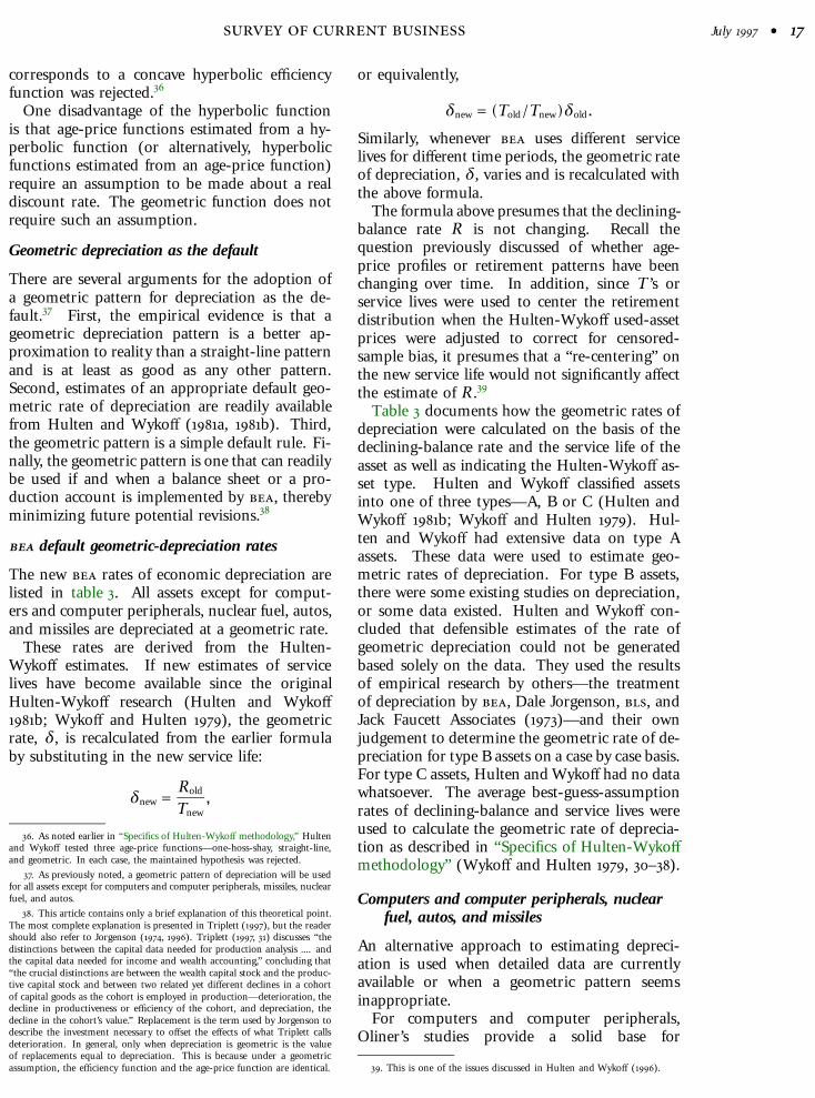
There are several arguments for the adoption ofa geometric pattern for depreciation as the de-fault. First, the empirical evidence is that ageometric depreciation pattern is a better ap-proximation to reality than a straight-line patternand is at least as good as any other pattern.Second, estimates of an appropriate default geo-metric rate of depreciation are readily availablefrom Hulten and Wykoff (a, b). Third,the geometric pattern is a simple default rule. Fi-nally, the geometric pattern is one that can readilybe used if and when a balance sheet or a pro-duction account is implemented by , therebyminimizing future potential revisions.

default geometric-depreciation rates

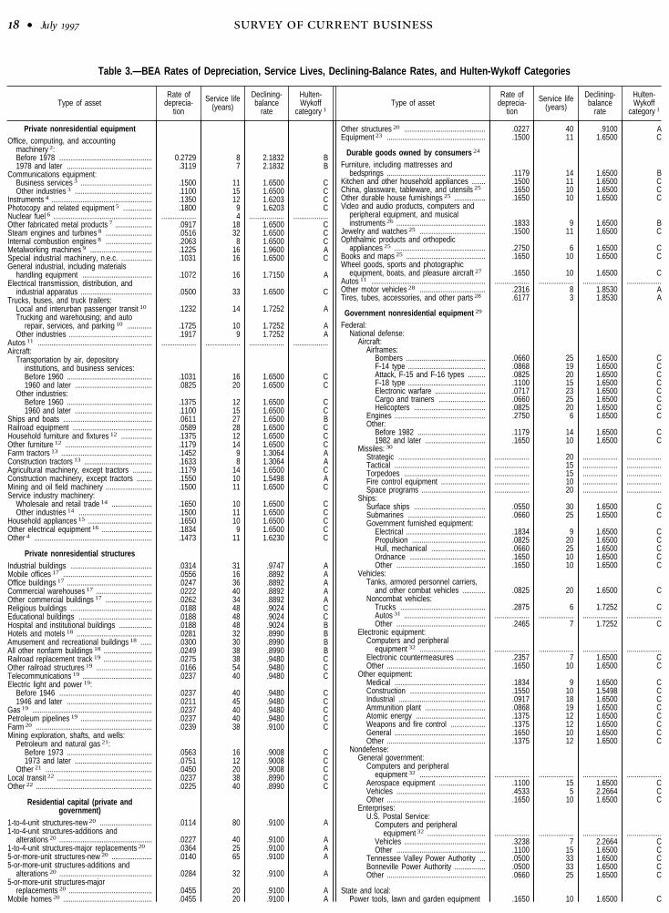
The new rates of economic depreciation arelisted in table . All assets except for comput-ers and computer peripherals, nuclear fuel, autos,and missiles are depreciated at a geometric rate.

These rates are derived from the Hulten-Wykoff estimates. If new estimates of servicelives have become available since the originalHulten-Wykoff research (Hulten and Wykoffb; Wykoff and Hulten ), the geometricrate, δ, is recalculated from the earlier formulaby substituting in the new service life:

δnew =Rold

Tnew,

. As noted earlier in “Specifics of Hulten-Wykoff methodology,” Hultenand Wykoff tested three age-price functions—one-hoss-shay, straight-line,and geometric. In each case, the maintained hypothesis was rejected.

. As previously noted, a geometric pattern of depreciation will be usedfor all assets except for computers and computer peripherals, missiles, nuclearfuel, and autos.

. This article contains only a brief explanation of this theoretical point.The most complete explanation is presented in Triplett (), but the readershould also refer to Jorgenson (, ). Triplett (, ) discusses “thedistinctions between the capital data needed for production analysis .... andthe capital data needed for income and wealth accounting,” concluding that“the crucial distinctions are between the wealth capital stock and the produc-tive capital stock and between two related yet different declines in a cohortof capital goods as the cohort is employed in production—deterioration, thedecline in productiveness or efficiency of the cohort, and depreciation, thedecline in the cohort’s value.” Replacement is the term used by Jorgenson todescribe the investment necessary to offset the effects of what Triplett callsdeterioration. In general, only when depreciation is geometric is the valueof replacements equal to depreciation. This is because under a geometricassumption, the efficiency function and the age-price function are identical.

or equivalently,

δnew = (Told/Tnew)δold.

Similarly, whenever uses different servicelives for different time periods, the geometric rateof depreciation, δ, varies and is recalculated withthe above formula.

The formula above presumes that the declining-balance rate R is not changing. Recall thequestion previously discussed of whether age-price profiles or retirement patterns have beenchanging over time. In addition, since T ’s orservice lives were used to center the retirementdistribution when the Hulten-Wykoff used-assetprices were adjusted to correct for censored-sample bias, it presumes that a “re-centering” onthe new service life would not significantly affectthe estimate of R.

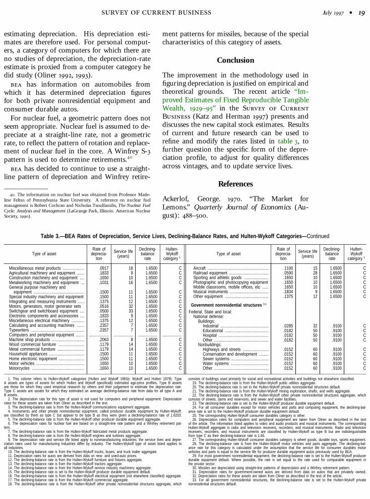
Table documents how the geometric rates ofdepreciation were calculated on the basis of thedeclining-balance rate and the service life of theasset as well as indicating the Hulten-Wykoff as-set type. Hulten and Wykoff classified assetsinto one of three types—A, B or C (Hulten andWykoff b; Wykoff and Hulten ). Hul-ten and Wykoff had extensive data on type Aassets. These data were used to estimate geo-metric rates of depreciation. For type B assets,there were some existing studies on depreciation,or some data existed. Hulten and Wykoff con-cluded that defensible estimates of the rate ofgeometric depreciation could not be generatedbased solely on the data. They used the resultsof empirical research by others—the treatmentof depreciation by , Dale Jorgenson, , andJack Faucett Associates ()—and their ownjudgement to determine the geometric rate of de-preciation for type B assets on a case by case basis.For type C assets, Hulten and Wykoff had no datawhatsoever. The average best-guess-assumptionrates of declining-balance and service lives wereused to calculate the geometric rate of deprecia-tion as described in “Specifics of Hulten-Wykoffmethodology” (Wykoff and Hulten , –).

Computers and computer peripherals, nuclearfuel, autos, and missiles

An alternative approach to estimating depreci-ation is used when detailed data are currentlyavailable or when a geometric pattern seemsinappropriate.

For computers and computer peripherals,Oliner’s studies provide a solid base for

. This is one of the issues discussed in Hulten and Wykoff ().

• July

Table 3.—BEA Rates of Depreciation, Service Lives, Declining-Balance Rates, and Hulten-Wykoff Categories

Type of assetRate of

deprecia-tion

Service life(years)

Declining-balance

rate

Hulten-Wykoff

category 1

Private nonresidential equipmentOffice, computing, and accounting

machinery 2:Before 1978 ................................................ 0.2729 8 2.1832 B1978 and later ............................................ .3119 7 2.1832 B

Communications equipment:Business services 3 ..................................... .1500 11 1.6500 COther industries 3 ........................................ .1100 15 1.6500 C

Instruments 4 .................................................... .1350 12 1.6203 CPhotocopy and related equipment 5 ............... .1800 9 1.6203 CNuclear fuel 6 ................................................... .................. 4 .................. ..................Other fabricated metal products 7 ................... .0917 18 1.6500 CSteam engines and turbines 8 ........................ .0516 32 1.6500 CInternal combustion engines 8 ........................ .2063 8 1.6500 CMetalworking machines 9 ................................ .1225 16 1.9600 ASpecial industrial machinery, n.e.c. ................ .1031 16 1.6500 CGeneral industrial, including materials

handling equipment .................................... .1072 16 1.7150 AElectrical transmission, distribution, and

industrial apparatus ..................................... .0500 33 1.6500 CTrucks, buses, and truck trailers:

Local and interurban passenger transit 10 .1232 14 1.7252 ATrucking and warehousing; and auto

repair, services, and parking 10 ............. .1725 10 1.7252 AOther industries ........................................... .1917 9 1.7252 A

Autos 11 ........................................................... .................. .................. .................. ..................Aircraft:

Transportation by air, depositoryinstitutions, and business services:Before 1960 ............................................ .1031 16 1.6500 C1960 and later ........................................ .0825 20 1.6500 C

Other industries:Before 1960 ............................................ .1375 12 1.6500 C1960 and later ........................................ .1100 15 1.6500 C

Ships and boats .............................................. .0611 27 1.6500 BRailroad equipment ......................................... .0589 28 1.6500 CHousehold furniture and fixtures 12 ................ .1375 12 1.6500 COther furniture 12 ............................................. .1179 14 1.6500 CFarm tractors 13 ............................................... .1452 9 1.3064 AConstruction tractors 13 ................................... .1633 8 1.3064 AAgricultural machinery, except tractors .......... .1179 14 1.6500 CConstruction machinery, except tractors ........ .1550 10 1.5498 AMining and oil field machinery ........................ .1500 11 1.6500 CService industry machinery:

Wholesale and retail trade 14 ..................... .1650 10 1.6500 COther industries 14 ...................................... .1500 11 1.6500 C

Household appliances 15 ................................. .1650 10 1.6500 COther electrical equipment 16 .......................... .1834 9 1.6500 COther 4 ............................................................. .1473 11 1.6230 C

Private nonresidential structuresIndustrial buildings .......................................... .0314 31 .9747 AMobile offices 17 .............................................. .0556 16 .8892 AOffice buildings 17 ............................................ .0247 36 .8892 ACommercial warehouses 17 ............................. .0222 40 .8892 AOther commercial buildings 17 ........................ .0262 34 .8892 AReligious buildings .......................................... .0188 48 .9024 CEducational buildings ...................................... .0188 48 .9024 CHospital and institutional buildings ................. .0188 48 .9024 BHotels and motels 18 ....................................... .0281 32 .8990 BAmusement and recreational buildings 18 ...... .0300 30 .8990 BAll other nonfarm buildings 18 ......................... .0249 38 .8990 BRailroad replacement track 19 ......................... .0275 38 .9480 COther railroad structures 19 ............................. .0166 54 .9480 CTelecommunications 19 .................................... .0237 40 .9480 CElectric light and power 19:

Before 1946 ................................................ .0237 40 .9480 C1946 and later ............................................ .0211 45 .9480 C

Gas 19 .............................................................. .0237 40 .9480 CPetroleum pipelines 19 ..................................... .0237 40 .9480 CFarm 20 ............................................................ .0239 38 .9100 CMining exploration, shafts, and wells:

Petroleum and natural gas 21:Before 1973 ............................................ .0563 16 .9008 C1973 and later ........................................ .0751 12 .9008 C

Other 21 ....................................................... .0450 20 .9008 CLocal transit 22 ................................................. .0237 38 .8990 COther 22 ............................................................ .0225 40 .8990 C

Residential capital (private andgovernment)

1-to-4-unit structures-new 20 ........................... .0114 80 .9100 A1-to-4-unit structures-additions and

alterations 20 ................................................ .0227 40 .9100 A1-to-4-unit structures-major replacements 20 .0364 25 .9100 A5-or-more-unit structures-new 20 ..................... .0140 65 .9100 A5-or-more-unit structures-additions and

alterations 20 ................................................ .0284 32 .9100 A5-or-more-unit structures-major

replacements 20 ........................................... .0455 20 .9100 AMobile homes 20 .............................................. .0455 20 .9100 A

Type of assetRate of

deprecia-tion

Service life(years)

Declining-balance

rate

Hulten-Wykoff

category 1

Other structures 20 .......................................... .0227 40 .9100 AEquipment 23 ................................................... .1500 11 1.6500 C

Durable goods owned by consumers 24

Furniture, including mattresses andbedsprings ................................................... .1179 14 1.6500 B

Kitchen and other household appliances ....... .1500 11 1.6500 CChina, glassware, tableware, and utensils 25 .1650 10 1.6500 COther durable house furnishings 25 ................ .1650 10 1.6500 CVideo and audio products, computers and

peripheral equipment, and musicalinstruments 26 .............................................. .1833 9 1.6500 B

Jewelry and watches 25 .................................. .1500 11 1.6500 COphthalmic products and orthopedic

appliances 25 ............................................... .2750 6 1.6500 CBooks and maps 25 ......................................... .1650 10 1.6500 CWheel goods, sports and photographic

equipment, boats, and pleasure aircraft 27 .1650 10 1.6500 CAutos 11 ........................................................... .................. .................. .................. ..................Other motor vehicles 28 .................................. .2316 8 1.8530 ATires, tubes, accessories, and other parts 28 .6177 3 1.8530 A

Government nonresidential equipment 29

Federal:National defense:

Aircraft:Airframes:

Bombers ......................................... .0660 25 1.6500 CF-14 type ........................................ .0868 19 1.6500 CAttack, F-15 and F-16 types ......... .0825 20 1.6500 CF-18 type ........................................ .1100 15 1.6500 CElectronic warfare .......................... .0717 23 1.6500 CCargo and trainers ........................ .0660 25 1.6500 CHelicopters ..................................... .0825 20 1.6500 C

Engines ............................................... .2750 6 1.6500 COther:

Before 1982 ................................... .1179 14 1.6500 C1982 and later ............................... .1650 10 1.6500 C

Missiles: 30

Strategic ............................................. .................. 20 .................. ..................Tactical ............................................... .................. 15 .................. ..................Torpedoes .......................................... .................. 15 .................. ..................Fire control equipment ....................... .................. 10 .................. ..................Space programs ................................. .................. 20 .................. ..................

Ships:Surface ships ..................................... .0550 30 1.6500 CSubmarines ........................................ .0660 25 1.6500 CGovernment furnished equipment:

Electrical ......................................... .1834 9 1.6500 CPropulsion ...................................... .0825 20 1.6500 CHull, mechanical ............................ .0660 25 1.6500 COrdnance ....................................... .1650 10 1.6500 COther .............................................. .1650 10 1.6500 C

Vehicles:Tanks, armored personnel carriers,

and other combat vehicles ............ .0825 20 1.6500 CNoncombat vehicles:

Trucks ............................................ .2875 6 1.7252 CAutos 31 .......................................... .................. .................. .................. ..................Other .............................................. .2465 7 1.7252 C

Electronic equipment:Computers and peripheral

equipment 32 .................................. .................. .................. .................. ..................Electronic countermeasures ............... .2357 7 1.6500 COther ................................................... .1650 10 1.6500 C

Other equipment:Medical ............................................... .1834 9 1.6500 CConstruction ....................................... .1550 10 1.5498 CIndustrial ............................................. .0917 18 1.6500 CAmmunition plant ............................... .0868 19 1.6500 CAtomic energy .................................... .1375 12 1.6500 CWeapons and fire control .................. .1375 12 1.6500 CGeneral ............................................... .1650 10 1.6500 COther ................................................... .1375 12 1.6500 C

Nondefense:General government:

Computers and peripheralequipment 32 .................................. .................. .................. .................. ..................

Aerospace equipment ........................ .1100 15 1.6500 CVehicles .............................................. .4533 5 2.2664 COther ................................................... .1650 10 1.6500 C

Enterprises:U.S. Postal Service:

Computers and peripheralequipment 32 .............................. .................. .................. .................. ..................

Vehicles .......................................... .3238 7 2.2664 COther .............................................. .1100 15 1.6500 C

Tennessee Valley Power Authority ... .0500 33 1.6500 CBonneville Power Authority ................ .0500 33 1.6500 COther ................................................... .0660 25 1.6500 C

State and local:Power tools, lawn and garden equipment .1650 10 1.6500 C

July •

estimating depreciation. His depreciation esti-mates are therefore used. For personal comput-ers, a category of computers for which there areno studies of depreciation, the depreciation-rateestimate is proxied from a computer category hedid study (Oliner , ).

has information on automobiles fromwhich it has determined depreciation figuresfor both private nonresidential equipment andconsumer durable autos.

For nuclear fuel, a geometric pattern does notseem appropriate. Nuclear fuel is assumed to de-preciate at a straight-line rate, not a geometricrate, to reflect the pattern of rotation and replace-ment of nuclear fuel in the core. A Winfrey S-pattern is used to determine retirements.

has decided to continue to use a straight-line pattern of depreciation and Winfrey retire-

. The information on nuclear fuel was obtained from Professor Made-line Feltus of Pennsylvania State University. A reference on nuclear fuelmanagement is Robert Cochran and Nicholas Tsoulfanidis, The Nuclear FuelCycle: Analysis and Management (LaGrange Park, Illinois: American NuclearSociety, ).

Table 3.—BEA Rates of Depreciation, Service Liv

Type of assetRate of

deprecia-tion

Service life(years)

Declining-balance

rate

Miscellaneous metal products .................... .0917 18 1.6500Agricultural machinery and equipment ....... .1833 9 1.6500Construction machinery and equipment .... .1650 10 1.6500Metalworking machinery and equipment ... .1031 16 1.6500General purpose machinery and

equipment ............................................... .1500 11 1.6500Special industry machinery and equipment .1500 11 1.6500Integrating and measuring instruments ...... .1375 12 1.6500Motors, generators, motor generator sets .0516 32 1.6500Switchgear and switchboard equipment .... .0500 33 1.6500Electronic components and accessories .... .1833 9 1.6500Miscellaneous electrical machinery ............ .1375 12 1.6500Calculating and accounting machines ....... .2357 7 1.6500Typewriters .................................................. .2357 7 1.6500Computers and peripheral equipment ........ .................. .................. ..................Machine shop products .............................. .2063 8 1.6500Wood commercial furniture ........................ .1179 14 1.6500Metal commercial furniture ......................... .1179 14 1.6500Household appliances ................................. .1500 11 1.6500Home electronic equipment ........................ .1500 11 1.6500Motor vehicles ............................................. .1650 10 1.6500Motorcycles ................................................. .1650 10 1.6500

1. This column refers to Hulten-Wykoff categories (Hulten and Wykoff 1981b; Wykoff and HulteA assets are types of assets for which Hulten and Wykoff specifically estimated age-price profiles. are those for which they used empirical research by others and their judgement to estimate the deType C assets are assets for which they estimated an average declining-balance rate from data for B assets.

2. The depreciation rate for this type of asset is not used for computers and peripheral equipmenrates for these assets are taken from Oliner as described in the text.

3. The declining-balance rate is from the Hulten-Wykoff communications equipment aggregate.4. Instruments and other private nonresidential equipment, called producer durable equipment by

are classified by them as type C but appear to be type B as they were given a declining-balance 5. The declining-balance rate is from the Hulten-Wykoff other producer durable equipment aggregate6. The depreciation rates for nuclear fuel are based on a straight-line rate pattern and a Winfrey

tern.7. The declining-balance rate is from the Hulten-Wykoff fabricated metal products aggregate.8. The declining-balance rate is from the Hulten-Wykoff engines and turbines aggregate.9. The depreciation rate and service life listed apply to nonmanufacturing industries; the service li

ciation rates used for manufacturing industries differ by industry. The Hulten-Wykoff type of asset liall industries.

10. The declining-balance rate is from the Hulten-Wykoff trucks, buses, and truck trailer aggregate.11. Depreciation rates for autos are derived from data on new- and used-auto prices.12. The declining-balance rate is from the Hulten-Wykoff furniture and fixtures aggregate.13. The declining-balance rate is from the Hulten-Wykoff tractors aggregate.14. The declining-balance rate is from the Hulten-Wykoff service industry machinery aggregate.15. The declining-balance rate is set to the Hulten-Wykoff producer durable equipment default.16. The declining-balance rate is from the Hulten-Wykoff electrical equipment (not elsewhere classif17. The declining-balance rate is from the Hulten-Wykoff commercial aggregate.18. The declining-balance rate is from the Hulten-Wykoff other private nonresidential structures ag

ment patterns for missiles, because of the specialcharacteristics of this category of assets.

Conclusion

The improvement in the methodology used infiguring depreciation is justified on empirical andtheoretical grounds. The recent article “Im-proved Estimates of Fixed Reproducible TangibleWealth, –” in the S CB (Katz and Herman ) presents anddiscusses the new capital stock estimates. Resultsof current and future research can be used torefine and modify the rates listed in table , tofurther question the specific form of the depre-ciation profile, to adjust for quality differencesacross vintages, and to update service lives.

References

Ackerlof, George. . “The Market forLemons.” Quarterly Journal of Economics (Au-gust): –.

es, Declining-Balance Rates, and Hulten-Wykoff Categories—Continued

Hulten-Wykoff

category 1

CCCC

CCCCCCCCC

..................CCCCCCC

Type of assetRate of

deprecia-tion

Service life(years)

Declining-balance

rate

Hulten-Wykoff

category 1

Aircraft ......................................................... .1100 15 1.6500 CRailroad equipment ..................................... .0590 28 1.6500 CSporting and athletic goods ....................... .1650 10 1.6500 CPhotographic and photocopying equipment .1650 10 1.6500 CMobile classrooms, mobile offices, etc ...... .1650 10 1.6500 CMusical instruments .................................... .1834 9 1.6500 COther equipment ......................................... .1375 12 1.6500 C

Government nonresidential structures 33

Federal, State and local:National defense:

Buildings:Industrial ............................................. .0285 32 .9100 CEducational ......................................... .0182 50 .9100 CHospital ............................................... .0182 50 .9100 COther ................................................... .0182 50 .9100 C

Nonbuildings:Highways and streets ........................ .0152 60 .9100 CConservation and development ......... .0152 60 .9100 CSewer systems ................................... .0152 60 .9100 CWater systems ................................... .0152 60 .9100 COther ................................................... .0152 60 .9100 C

n 1979). TypeType B assetspreciation rate.all type A and

t. Depreciation

Hulten-Wykoff,rate of 1.6203..retirement pat-

ves and depre-sted applies to

ied) aggregate.

gregate, which

consists of buildings used primarily for social and recreational activities and buildings not elsewhere classified.19. The declining-balance rate is from the Hulten-Wykoff public utilities aggregate.20. The declining-balance rate is set to the Hulten-Wykoff private nonresidential structures default.21. The declining-balance rate is from the Hulten-Wykoff mining exploration, shafts, and wells aggregate.22. The declining-balance rate is from the Hulten-Wykoff other private nonresidential structures aggregate, which

consists of streets, dams and reservoirs, and sewer and water facilities.23. The declining-balance rate is set to the Hulten-Wykoff producer durable equipment default.24. For all consumer durables except for motor vehicles and parts and computing equipment, the declining-bal-

ance rate is set to the Hulten-Wykoff producer durable equipment default.25. The corresponding Hulten-Wykoff consumer durables category is other.26. Depreciation rates for computers and peripheral equipment are taken from Oliner as described in the text

of the article. The information listed applies to video and audio products and musical instruments. The correspondingHulten-Wykoff aggregate is radio and television receivers, recorders, and musical instruments. Radio and televisionreceivers, recorders, and musical instruments are classified by Hulten-Wykoff as type B but are indistinguishablefrom type C as their declining-balance rate is 1.65.

27. The corresponding Hulten-Wykoff consumer durables category is wheel goods, durable toys, sports equipment.28. The declining-balance rate is from the Hulten-Wykoff motor vehicles and parts aggregate. The declining-bal-

ance rate for this category is calculated under the assumption that the service life for consumer durables motorvehicles and parts is equal to the service life for producer durable equipment autos previously used by BEA.

29. For most government nonresidential equipment, the declining-balance rate is set to the Hulten-Wykoff producerdurable equipment default. Where possible, the rate is set equal to the rate used for comparable equipment inthe private sector.

30. Missiles are depreciated using straight-line patterns of depreciation and a Winfrey retirement pattern.31. Depreciation rates for government-owned autos are derived from data on autos that are privately owned.32. Depreciation rates for these assets are taken from Oliner as described in the text of the article.33. For all government nonresidential structures, the declining-balance rate is set to the Hulten-Wykoff private

nonresidential structures default.

• July

Ackerman, Susan Rose. . “Used Cars asa Depreciating Asset.” Western Economic Journal(December): –.

Baily, Martin N. . “Productivity and theServices of Capital and Labor.” In BrookingsPapers on Economic Activity, vol. : –.

Bar-Yosef, Sasson, and Steven Lustgarten..“Economic Depreciation, Accounting De-preciation, and Their Relation to Current CostAccounting.” Journal of Accounting, Auditing andFinance , no. (Winter): –.

Beidleman, Carl R. . “Economic Deprecia-tion in a Capital Goods Industry.” National TaxJournal , no. (December): –.

Boskin, Michael J., Marc S. Robinson, and JohnM. Roberts. . “New Estimates of FederalGovernment Tangible Capital and Net Invest-ment.” In Technology and Capital Formation,edited by Dale W. Jorgenson and Ralph Landau,–. Cambridge: Press.

Box, George E.P., and David R. Cox. . “AnAnalysis of Transformations.”Journal of the RoyalStatistical Society, Series B , no. :–.

Brazell, David W., Lowell Dworin, and MichaelWalsh. . A History of Federal Tax Depreci-ation Policy. U.S. Department of the Treasury,Office of Tax Analysis Paper No. . Washington,: Office of Tax Analysis, May.

Bureau of Economic Analysis (), U.S. De-partment of Commerce. . Fixed ReproducibleTangible Wealth in the United States, –.Washington, : U.S. Government PrintingOffice, January.

Bureau of Labor Statistics (), U.S. Depart-ment of Labor. . Trends in MultifactorProductivity, –. Bulletin . Washington,: U.S. Government Printing Office, September.

. n.d. “Choice of Efficiency Func-tion.” Washington, : Office of Productivityand Technology.

Cagan, Phillip. . “Measuring QualityChanges and the Purchasing Power of Money:An Exploratory Study of Automobiles.” InPrice Indexes and Quality Change, edited byZvi Griliches, –. Cambridge: HarvardUniversity Press.

Cartwright, David W. . “Improved De-flation of Purchases of Computers,” S C B (March): –.

Chinloy, Peter. . “Hedonic Price andDepreciation Indexes for Residential Housing:A Longitudinal Approach.” Journal of UrbanEconomics :–.

Chow, Gregory C. . The Demand for Au-tomobiles in the United States. Amsterdam, TheNetherlands: North Holland.

. .“Statistical Demand Func-tions for Automobiles and Their Use for Fore-casting.” In The Demand for Durable Goods,edited by Arnold Harberger, –. Chicago:University of Chicago Press.

Cockburn, Iain, and Murray Frank. .“Market Conditions and Retirement of PhysicalCapital: Evidence From Oil Tankers.” Pa-per presented at the Workshop on the Meas-urement of Depreciation and Capital Stock atthe Conference on Research in Income andWealth, National Bureau of Economic Research,Washington, , June , .

Coen, Robert. . “Investment Behav-ior: The Measurement of Depreciation and TaxPolicy.”American Economic Review (March):–.

. . “Depreciation, Profits, andRates of Return in Manufacturing Industries.”In The Measurement of Capital. Studies in In-come and Wealth, vol. , edited by Dan Usher,–. Chicago: University of Chicago Press, forthe National Bureau of Economic Research.

DeLeeuw, Frank. . “Discussion.” InDepreciation, Inflation, and the Taxation of In-come From Capital, edited by Charles R. Hulten,–. Washington, : The Urban InstitutePress.

Denison, Edward F. . “Theoretical Aspectsof Quality Change, Capital Consumption, andNet Capital Formation.” In Problems of CapitalFormation: Concepts, Measurement, and Control-ling Factors. Studies in Income and Wealth,vol. , edited by Franco Modigliani, –.Princeton: Princeton University Press.

Doms, Mark E. . “Estimating Capital Effi-ciency Schedules Within Production Functions.”Economic Inquiry (January): –.

Downs, Thomas W., and Keith A. Shriver.. “The Analytical Derivation and Empiri-cal Test of a Tax-Adjusted Fundamental ValueModel.” Journal of Accounting Research ,Supplement: –.

Fabricant, Solomon. . Capital Consump-tion and Adjustment. New York: NationalBureau of Economic Research.

Faucett, Jack G. . “Development of CapitalStock Series by Industry Sector.” Washington,: U.S. Office of Emergency Preparedness.

Feldstein, Martin S., and Michael Rothschild.. “Towards an Economic Theory of Replace-

July •

ment Investment.” Econometrica , no. (May):–.

Griliches, Zvi. . “The Demand for aDurable Input: U.S. Farm Tractors, –.”In The Demand for Durable Goods, edited byArnold Harberger, –. Chicago: Universityof Chicago Press.

Gullickson, William, and Michael Harper. .“Multifactor Productivity in U.S. Manufactur-ing, –.” Monthly Labor Review (October):–.

Hall, Robert E. . “The Measurement ofQuality Changes from Vintage Price Data.” InPrice Indexes and Quality Change, edited byZvi Griliches, –. Cambridge: HarvardUniversity Press.

Harper, Michael J. . “The Measurementof Productive Capital Stock, Capital Wealth, andCapital Services.” Bureau of Labor StatisticsWorking Paper . Washington, : Bureau ofLabor Statistics, June.

Hulten, Charles R., and Frank C. Wykoff.a. “The Estimation of Economic Depreci-ation Using Vintage Asset Prices.” Journal ofEconometrics (April): –.

. b. “The Measurement of Eco-nomic Depreciation.” In Depreciation, Inflation,and the Taxation of Income from Capital, editedby Charles R. Hulten, –. Washington, :The Urban Institute Press.

. . “Issues in the Measure-ment of Economic Depreciation: IntroductoryRemarks.” Economic Inquiry (January): –.

Hulten, Charles R., James W. Robertson, andFrank C. Wykoff. . “Energy, Obsolescence,and the Productivity Slowdown.” In Technologyand Capital Formation, edited by Dale W. Jor-genson and Ralph Landau, –. Cambridge: Press.

Jorgenson, Dale W. .“The Economic The-ory of Replacement and Depreciation.” In Econo-metrics and Economic Theory, edited by WillySellekaerts, –. London: Macmillan.

. . “Capital as a Factor of Pro-duction.” In Technology and Capital Formation,edited by Dale W. Jorgenson and Ralph Landau,–. Cambridge, : Press.

. . “Empirical Studies of De-preciation.” Economic Inquiry (January):–.

Jorgenson, Dale W., and Kevin Stiroh. .“Investment in Computers and U.S. EconomicGrowth.” Cambridge, : Harvard UniversityDepartment of Economics.

Katz, Arnold J., and Shelby W. Herman. .“Improved Estimates of Fixed Reproducible Tan-gible Wealth, –.” S CB (May): –.

Koumanakos, Peter, and J.C. Hwang. .“The Forms and Rates of Economic Depreciation:The Canadian Experience.” Paper presented atthe th anniversary meeting of the Conferenceon Research in Income and Wealth, Washington,, May –, .

Lee, Bun Song. . “Measurement of CapitalDepreciation Within the Japanese Fishing Fleet.”Review of Economics and Statistics (May): –.

Malpezzi, Stephen, Larry Ozanne, and ThomasThibodeau. . “Microeconomic Estimates ofHousing Depreciation.” Land Economics , no. (November): –.

Marston, Anson, Robley Winfrey, and John C.Hempstead. . Engineering Valuation andDepreciation. Ames, Iowa: McGraw-Hill.

Nadiri, M. Ishaq, and Ingmar R. Prucha. .“Estimation of the Depreciation Rate of Physicaland Capital in the U.S. Total ManufacturingSector.” Economic Inquiry (January): –.

Office of Tax Analysis (). . “Report toCongress on the Depreciation of Scientific Instru-ments.” Washington, : Office of Tax Analysis,U.S. Department of the Treasury, March.

. a. “Report to Congress on theDepreciation of Business-Use Passenger Cars,”Washington, : Office of Tax Analysis, U.S.Department of the Treasury, April.

. b. “Report to Congress onthe Depreciation of Business-Use Light Trucks.”Washington, : Office of Tax Analysis, U.S.Department of the Treasury, September.

Ohta, Makoto, and Zvi Griliches. . “Au-tomobile Prices Revisited: Extensions of theHedonic Price Hypothesis.” In Household Pro-duction and Consumption. Studies in Income andWealth, vol. , edited by Nestor E. Terleckyj,–. Chicago: University of Chicago Press,for the National Bureau of Economic Research.

Oliner, Stephen D. . “Estimates of Depre-ciation and Retirement for Computer PeripheralEquipment.” Paper presented at the Workshopon the Measurement of Depreciation and CapitalStock at the Conference on Research in In-come and Wealth, National Bureau of EconomicResearch. Washington, , June , .

. . “Constant-Quality PriceChange, Depreciation, and Retirement of Main-frame Computers.” In Price Measurements andTheir Uses, edited by Murray F. Foss, Marilyn E.

• July

Manser, and Allan H. Young, –. Chicago:University of Chicago Press.

. . “Measuring Stocks of Com-puter Peripheral Equipment: Theory and Appli-cation.” Washington : Board of Governors ofthe Federal Reserve System, May.

. . “New Evidence on the De-preciation and Retirement of Machine Tools.”Economic Inquiry (January): –.

Parker, Robert P., and Jack E. Triplett. .“Preview of the Comprehensive Revision of theNational Income and Product Accounts: Recog-nition of Government Investment and Incorpo-ration of a New Methodology for CalculatingDepreciation.” S C B (September): –.

Penson, John B., Jr., Dean W. Hughes, andGlenn L. Nelson. . “Measurement of Ca-pacity Depreciation Based on Engineering Data.”American Journal of Agricultural Economics ,part (May): –.

Penson, John B., Jr., Robert F.J. Romain, andDean W. Hughes. . “Net Investment in FarmTractors: An Econometric Analysis.” Ameri-can Journal of Agricultural Economics , part (November): –.

Perry, Gregory M., and J. David Glyer. .“An Empirical Investigation of Depreciation Ratesfor Farm Tractors.” Corvallis: Oregon StateUniversity.

Powers, Susan G. . “The Role ofCapital Discards in Multifactor ProductivityMeasurement.” Monthly Labor Review (June)–.

Prucha, Igmar R., and M. Ishaq Nadiri.. “Endogenous Capital Utilization and Pro-ductivity Measurement in Dynamic Factor De-mand Models: Theory and Application to theU.S. Electrical Machinery Industry.” Journal ofEconometrics :–.

Ramm, Wolfhard. . “Measuring theServices of Household Durables: The Case of Au-tomobiles.” In Proceedings of the Business andEconomic Statistics Section of the American Sta-tistical Association, –. Washington, :American Statistical Association.

Russo, J.G., and H.A. Cowles. . “Revali-dation of the Iowa Type Survivor Curves.” TheEngineering Economist (Fall): –.

Shriver, Keith A. a. “A Statistical Test ofthe Stability Assumption Inherent in EmpiricalEstimates of Economic Depreciation.” Journal ofEconomic and Social Measurement :–.

. b. “The Valuation of CapitalAssets During Time Periods Exhibiting Alterna-

tive Degrees of Demand for Industrial Machineryand Equipment.” Journal of Economic and SocialMeasurement :–.

. . “The Estimation of Cur-rent Cost Depreciation,” Advances in Accounting:–.

. . “The Measurement ofCurrent Cost Data: Implications for EconomicAnalysis.” Journal of Economic and SocialMeasurement :–.

System of National Accounts, . . Com-mission of the European Communities, Inter-national Monetary Fund, Organisation for Eco-nomic Co-operation and Development, UnitedNations, World Bank. Brussels, Luxemborg,Paris, New York, Washington, .

Taubman, Paul, and Robert Rasche. .“Economic and Tax Depreciation of Office Build-ings.” National Tax Journal , no. (September):–.

. . “Subsidies, EconomicLives, and Complete Resource Misallocation.”American Economic Review (December):–.

Triplett, Jack E. . “Price and TechnologicalChange in a Capital Good.” in Technology andCapital Formation, edited by D.W. Jorgenson andR. Landau, –. Cambridge: Press.

. a. “A Fowler’s for Cap-ital: A ‘Mini-Directory’ of Usage on CapitalMeasurement.” Appendix to “Measuring theCapital Stock: A Review of Concepts and DataNeeds.” Paper presented at the Workshop on theMeasurement of Depreciation and Capital Stockat the Conference on Research in Income andWealth, National Bureau of Economic Research,Washington, , June , .

. b. “Measuring the Cap-ital Stock: A Review of Concepts and DataNeeds.” Paper presented at the Workshop on theMeasurement of Depreciation and Capital Stockat the Conference on Research in Income andWealth, National Bureau of Economic Research,Washington, , June , .

. . “Depreciation in ProductionAnalysis and in Income and Wealth Accounts:Resolution of an Old Debate.” Economic Inquiry (January): –.

. . “Concepts of Capital forProduction Accounts and for Wealth Accounts:The Implications for Statistical Programs.” Pa-per presented at the International Conferenceon Capital Stock Statistics, Canberra, Australia,March –, .

July •

Winfrey, Robert. . Statistical Analysisof Industrial Property Retirements. Bulletin ,Revised. Ames, Iowa: Engineering ResearchInstitute, Iowa State University.

Wykoff, Frank C. . “Capital Depreciationin the Postwar Period: Automobiles.” Review ofEconomics and Statistics (May): –.

. . “Economic Depreciation andthe User Cost of Business-Leased Automobiles.”In Technology and Capital Formation, editedby D.W. Jorgenson and R. Landau, –.Cambridge: Press.

Wykoff, Frank C., and Charles R. Hulten. .“Tax and Economic Depreciation of Machineryand Equipment: A Theoretical and Empirical Ap-praisal, Phase Report.” Economic Depreciationof the U.S. Capital Stock: A First Step. Washing-ton, : U.S. Department of the Treasury, Officeof Tax Analysis, July , .

Young, Allan H., and John C. Musgrave.. “Estimation of Capital Stock in the UnitedStates.” In The Measurement of Capital. Studiesin Income and Wealth, vol. , edited by DanUsher, –. Chicago: University of ChicagoPress.