The Maths Workbook - Abi Adams-Prassl
152
The Maths Workbook Oxford University Department of Economics The Maths Workbook has been developed for use by students preparing for the Preliminary Examination in PPE, E&M and History and Economics. It covers the mathematical tech- niques that students are expected to know for the exam. The Maths Workbook was written by Margaret Stevens, with the help of: Alan Beggs, David Foster, Mary Gregory, Ben Irons, Godfrey Keller, Sujoy Mukerji, Mathan Satchi, Patrick Wallace, Tania Wilson. c Margaret Stevens 2003 Complementary Textbooks As far as possible the Workbook is self-contained, but it should be used in conjunction with standard textbooks for a fuller coverage: • Malcolm Pemberton and Nicholas Rao Mathematics for Economists: An Introduc- tory Textbook 4th edition 2016, or earlier editions. (Comprehensive; appropriate level. This book is not included in the specific references in workbook chapters, but students should find it easy to identify relevant sections.) • Ian Jacques Mathematics for Economics and Business 7th Edition 2013, or earlier editions. (The most elementary.) • Martin Anthony and Norman Biggs Mathematics for Economics and Finance, 1996. (Useful and concise, but less suitable for students who have not previously studied mathematics to A-level.) • Carl P. Simon and Lawrence Blume Mathematics for Economists, 1994 or 2010. (A good but more advanced textbook, that goes well beyond the Workbook.) • Hal R. Varian Intermediate Microeconomics: A Modern Approach covers many of the economic applications, particularly in the Appendices to individual chapters, where calculus is used. • In addition, students who have not studied A-level maths, or feel that their maths is weak, may find it helpful to use one of the many excellent textbooks available for A-level Pure Mathematics (particularly the first three modules). How to Use the Workbook There are ten chapters, each of which can be used as the basis for a class. It is intended that students should be able to work through each chapter alone, doing the exercises and checking their own answers. References to some of the textbooks listed above are given at the end of each section. At the end of each chapter is a worksheet, the answers for which are available for the use of tutors only. The first two chapters are intended mainly for students who have not done A-level maths: they assume GCSE maths only. In subsequent chapters, students who have done A-level will find both familiar and new material.
-
Upload
khangminh22 -
Category
Documents
-
view
3 -
download
0
Transcript of The Maths Workbook - Abi Adams-Prassl

The Maths Workbook
Oxford University Department of Economics
The Maths Workbook has been developed for use by students preparing for the PreliminaryExamination in PPE, E&M and History and Economics. It covers the mathematical tech-niques that students are expected to know for the exam.
The Maths Workbook was written by Margaret Stevens, with the help of: Alan Beggs, DavidFoster, Mary Gregory, Ben Irons, Godfrey Keller, Sujoy Mukerji, Mathan Satchi, PatrickWallace, Tania Wilson.
c�Margaret Stevens 2003
Complementary TextbooksAs far as possible the Workbook is self-contained, but it should be used in conjunction withstandard textbooks for a fuller coverage:
• Malcolm Pemberton and Nicholas Rao Mathematics for Economists: An Introduc-tory Textbook 4th edition 2016, or earlier editions. (Comprehensive; appropriatelevel. This book is not included in the specific references in workbook chapters, butstudents should find it easy to identify relevant sections.)
• Ian Jacques Mathematics for Economics and Business 7th Edition 2013, or earliereditions. (The most elementary.)
• Martin Anthony and Norman Biggs Mathematics for Economics and Finance, 1996.(Useful and concise, but less suitable for students who have not previously studiedmathematics to A-level.)
• Carl P. Simon and Lawrence Blume Mathematics for Economists, 1994 or 2010. (Agood but more advanced textbook, that goes well beyond the Workbook.)
• Hal R. Varian Intermediate Microeconomics: A Modern Approach covers many ofthe economic applications, particularly in the Appendices to individual chapters,where calculus is used.
• In addition, students who have not studied A-level maths, or feel that their mathsis weak, may find it helpful to use one of the many excellent textbooks available forA-level Pure Mathematics (particularly the first three modules).
How to Use the WorkbookThere are ten chapters, each of which can be used as the basis for a class. It is intended thatstudents should be able to work through each chapter alone, doing the exercises and checkingtheir own answers. References to some of the textbooks listed above are given at the end ofeach section.
At the end of each chapter is a worksheet, the answers for which are available for the use oftutors only.
The first two chapters are intended mainly for students who have not done A-level maths:they assume GCSE maths only. In subsequent chapters, students who have done A-level willfind both familiar and new material.

Contents(1) Review of Algebra
Simplifying and factorising algebraic expressions; indices and logarithms; solvingequations (linear equations, equations involving parameters, changing the subject ofa formula, quadratic equations, equations involving indices and logs); simultaneousequations; inequalities and absolute value.
(2) Lines and GraphsThe gradient of a line, drawing and sketching graphs, linear graphs (y = mx+c), qua-dratic graphs, solving equations and inequalities using graphs, budget constraints.
(3) Sequences, Series and Limits; the Economics of FinanceArithmetic and geometric sequences and series; interest rates, savings and loans;present value; limit of a sequence, perpetuities; the number e, continuous com-pounding of interest.
(4) FunctionsCommon functions, limits of functions; composite and inverse functions; supply anddemand functions; exponential and log functions with economic applications; func-tions of several variables, isoquants; homogeneous functions, returns to scale.
(5) Di↵erentiationDerivative as gradient; di↵erentiating y = x
n; notation and interpretation of deriva-tives; basic rules and di↵erentiation of polynomials; economic applications: MC,MPL, MPC; stationary points; the second derivative, concavity and convexity.
(6) More Di↵erentiation, and OptimisationSketching graphs; cost functions; profit maximisation; product, quotient and chainrule; elasticities; di↵erentiating exponential and log functions; growth; the optimumtime to sell an asset.
(7) Partial Di↵erentiationFirst- and second-order partial derivatives; marginal products, Euler’s theorem; dif-ferentials; the gradient of an isoquant; indi↵erence curves, MRS and MRTS; thechain rule and implicit di↵erentiation; comparative statics.
(8) Unconstrained Optimisation Problems with One or More VariablesFirst- and second-order conditions for optimisation, Perfect competition and monop-oly; strategic optimisation problems: oligopoly, externalities; optimising functionsof two or more variables.
(9) Constrained OptimisationMethods for solving consumer choice problems: tangency condition and Lagrangian;cost minimisation; the method of Lagrange multipliers; other economic applications;demand functions.
(10) IntegrationIntegration as the reverse of di↵erentiation; rules for integration; areas and definiteintegrals; producer and consumer surplus; integration by substitution and by parts;integrals and sums; the present value of an income flow.

Errors and ImprovementsThe Workbook was completed in summer 2003. As far as possible, examples, exercises andanswers were carefully checked. Since then, a small number of errors have been corrected,and updated versions of the chapters placed on the Economics Department Weblearn site.Versions of each chapter are identified by the release date, which can be found on the pagecontaining the answers to the exercises (in most cases, the penultimate page).
Please report any mistakes that you notice, however small or large. Suggestions from tutorsand students for improvements to the Workbook are very welcome.
Margaret Stevens, September [email protected]

CHAPTER 1
Review of Algebra
Much of the material in this chapter is revision from GCSE maths (al-though some of the exercises are harder). Some of it – particularly thework on logarithms – may be new if you have not done A-level maths.If you have done A-level, and are confident, you can skip most of the ex-ercises and just do the worksheet, using the chapter for reference wherenecessary.
—./—↵⌦
� 1. Algebraic Expressions
1.1. Evaluating Algebraic Expressions
Examples 1.1:
(i) A firm that manufactures widgets has m machines and employs n workers. The numberof widgets it produces each day is given by the expression m
2(n�3). How many widgetsdoes it produce when m = 5 and n = 6?
Number of widgets = 52 ⇥ (6� 3) = 25⇥ 3 = 75
(ii) In another firm, the cost of producing x widgets is given by 3x2 + 5x+ 4. What is thecost of producing (a) 10 widgets (b) 1 widget?
When x = 10, cost = (3⇥ 102) + (5⇥ 10) + 4 = 300 + 50 + 4 = 354
When x = 1, cost = 3⇥ 12 + 5⇥ 1 + 4 = 3 + 5 + 4 = 12It might be clearer to use brackets here, but they are not essential:
the rule is that ⇥ and ÷ are evaluated before + and �.
(iii) Evaluate the expression 8y4 � 126�y
when y = �2.
(Remember that y4 means y ⇥ y ⇥ y ⇥ y.)
8y4 �12
6� y
= 8⇥ (�2)4 �12
6� (�2)= 8⇥ 16�
12
8= 128� 1.5 = 126.5
(If you are uncertain about using negative numbers, work through Jacques pp.7–9.)
Exercises 1.1: Evaluate the following expressions when x = 1, y = 3, z = �2 and t = 0:(a) 3y2 � z (b) xt+ z
3 (c) (x+ 3z)y (d) y
z
+ 2x
(e) (x+ y)3 (f) 5� x+32t�z
1

2 1. REVIEW OF ALGEBRA
1.2. Manipulating and Simplifying Algebraic Expressions
Examples 1.2:
(i) Simplify 1 + 3x� 4y + 3xy + 5y2 + y � y
2 + 4xy � 8.This is done by collecting like terms, and adding them together:
1 + 3x� 4y + 3xy + 5y2 + y � y
2 + 4xy � 8
= 5y2 � y
2 + 3xy + 4xy + 3x� 4y + y + 1� 8
= 4y2 + 7xy + 3x� 3y � 7
The order of the terms in the answer doesn’t matter, but we often put a positive termfirst, and/or write “higher-order” terms such as y2 before “lower-order” ones such as yor a number.
(ii) Simplify 5(x� 3)� 2x(x+ y � 1).Here we need to multiply out the brackets first, and then collect terms:
5(x� 3)� 2x(x+ y � 1) = 5x� 15� 2x2 � 2xy + 2x
= 7x� 2x2 � 2xy � 15
(iii) Multiply x
3 by x
2.
x
3⇥ x
2 = x⇥ x⇥ x⇥ x⇥ x = x
5
(iv) Divide x
3 by x
2.We can write this as a fraction, and cancel:
x
3÷ x
2 =x⇥ x⇥ x
x⇥ x
=x
1= x
(v) Multiply 5x2y4 by 4yx6.
5x2y4 ⇥ 4yx6 = 5⇥ x
2⇥ y
4⇥ 4⇥ y ⇥ x
6
= 20⇥ x
8⇥ y
5
= 20x8y5
Note that you can always change the order of multiplication.
(vi) Divide 6x2y3 by 2yx5.
6x2y3 ÷ 2yx5 =6x2y3
2yx5=
3x2y3
yx
5=
3y3
yx
3
=3y2
x
3
(vii) Add 3xy
and y
2 .The rules for algebraic fractions are just the same as for numbers, so here we find acommon denominator :
3x
y
+y
2=
6x
2y+
y
2
2y
=6x+ y
2
2y

1. REVIEW OF ALGEBRA 3
(viii) Divide 3x2
y
by xy
3
2 .
3x2
y
÷
xy
3
2=
3x2
y
⇥
2
xy
3=
3x2 ⇥ 2
y ⇥ xy
3=
6x2
xy
4
=6x
y
4
Exercises 1.2: Simplify the following as much as possible:
(1)(1) (a) 3x� 17 + x
3 + 10x� 8 (b) 2(x+ 3y)� 2(x+ 7y � x
2)
(2) (a) z2x� (z + 1) + z(2xz + 3) (b) (x+ 2)(x+ 4) + (3� x)(x+ 2)
(3) (a)3x2y
6x(b)
12xy3
2x2y2
(4) (a) 2x2 ÷ 8xy (b) 4xy ⇥ 5x2y3
(5) (a)2x
y
⇥
y
2
2x(b)
2x
y
÷
y
2
2x
(6) (a)2x+ 1
4+
x
3(b)
1
x� 1�
1
x+ 1(giving the answers as a single fraction)
1.3. Factorising
A number can be written as the product of its factors. For example: 30 = 5⇥ 6 = 5⇥ 3⇥ 2.Similarly “factorise” an algebraic expression means “write the expression as the product oftwo (or more) expressions.” Of course, some numbers (primes) don’t have any proper factors,and similarly, some algebraic expressions can’t be factorised.
Examples 1.3:
(i) Factorise 6x2 + 15x.Here, 3x is a common factor of each term in the expression so:
6x2 + 15x = 3x(2x+ 5)
The factors are 3x and (2x + 5). You can check the answer by multiplying out thebrackets.
(ii) Factorise x
2 + 2xy + 3x+ 6y.There is no common factor of all the terms but the first pair have a common factor,and so do the second pair, and this leads us to the factors of the whole expression:
x
2 + 2xy + 3x+ 6y = x(x+ 2y) + 3(x+ 2y)
= (x+ 3)(x+ 2y)
Again, check by multiplying out the brackets.
(iii) Factorise x
2 + 2xy + 3x+ 3y.We can try the method of the previous example, but it doesn’t work. The expressioncan’t be factorised.

4 1. REVIEW OF ALGEBRA
(iv) Simplify 5(x2 + 6x+ 3)� 3(x2 + 4x+ 5).Here we can first multiply out the brackets, then collect like terms, then factorise:
5(x2 + 6x+ 3)� 3(x2 + 4x+ 5) = 5x2 + 30x+ 15� 3x2 � 12x� 15
= 2x2 + 18x
= 2x(x+ 9)
Exercises 1.3: Factorising
(1)(1) Factorise: (a) 3x+ 6xy (b) 2y2 + 7y (c) 6a+ 3b+ 9c
(2) Simplify and factorise: (a) x(x2 + 8) + 2x2(x� 5)� 8x (b) a(b+ c)� b(a+ c)
(3) Factorise: xy + 2y + 2xz + 4z
(4) Simplify and factorise: 3x(x+ 4x
)� 4(x2 + 3) + 2x
1.4. Polynomials
Expressions such as
5x2 � 9x4 � 20x+ 7 and 2y5 + y
3� 100y2 + 1
are called polynomials. A polynomial in x is a sum of terms, and each term is either a powerof x (multiplied by a number called a coe�cient), or just a number known as a constant. Allthe powers must be positive integers. (Remember: an integer is a positive or negative wholenumber.) The degree of the polynomial is the highest power. A polynomial of degree 2 iscalled a quadratic polynomial.
Examples 1.4: Polynomials
(i) 5x2 � 9x4 � 20x+ 7 is a polynomial of degree 4. In this polynomial, the coe�cient ofx
2 is 5 and the coe�cient of x is �20. The constant term is 7.
(ii) x
2 + 5x+ 6 is a quadratic polynomial. Here the coe�cient of x2 is 1.
1.5. Factorising Quadratics
In section 1.3 we factorised a quadratic polynomial by finding a common factor of each term:6x2 + 15x = 3x(2x+ 5). But this only works because there is no constant term. Otherwise,we can try a di↵erent method:
Examples 1.5: Factorising Quadratics
(i) x
2 + 5x+ 6• Look for two numbers that multiply to give 6, and add to give 5:
2⇥ 3 = 6 and 2 + 3 = 5
• Split the “x”-term into two:
x
2 + 2x+ 3x+ 6
• Factorise the first pair of terms, and the second pair:
x(x+ 2) + 3(x+ 2)

1. REVIEW OF ALGEBRA 5
• (x+ 2) is a factor of both terms so we can rewrite this as:
(x+ 3)(x+ 2)
• So we have:
x
2 + 5x+ 6 = (x+ 3)(x+ 2)
(ii) y
2� y � 12
In this example the two numbers we need are 3 and �4, because 3⇥ (�4) = �12 and3 + (�4) = �1. Hence:
y
2� y � 12 = y
2 + 3y � 4y � 12
= y(y + 3)� 4(y + 3)
= (y � 4)(y + 3)
(iii) 2x2 � 5x� 12This example is slightly di↵erent because the coe�cient of x2 is not 1.
• Start by multiplying together the coe�cient of x2 and the constant:
2⇥ (�12) = �24
• Find two numbers that multiply to give �24, and add to give �5.
3⇥ (�8) = �24 and 3 + (�8) = �5
• Proceed as before:
2x2 � 5x� 12 = 2x2 + 3x� 8x� 12
= x(2x+ 3)� 4(2x+ 3)
= (x� 4)(2x+ 3)
(iv) x
2 + x� 1The method doesn’t work for this example, because we can’t see any numbers thatmultiply to give �1, but add to give 1. (In fact there is a pair of numbers that doesso, but they are not integers so we are unlikely to find them.)
(v) x
2� 49
The two numbers must multiply to give �49 and add to give zero. So they are 7 and�7:
x
2� 49 = x
2 + 7x� 7x� 49
= x(x+ 7)� 7(x+ 7)
= (x� 7)(x+ 7)
The last example is a special case of the result known as “the di↵erence of two squares”. Ifa and b are any two numbers:
a
2� b
2 = (a� b)(a+ b)
Exercises 1.4: Use the method above (if possible) to factorise the following quadratics:
(1)(1) x
2 + 4x+ 3
(2) y
2 + 10� 7y
(3) 2x2 + 7x+ 3
(4) z
2 + 2z � 15
(5) 4x2 � 9
(6) y
2� 10y + 25
(7) x
2 + 3x+ 1

6 1. REVIEW OF ALGEBRA
1.6. Rational Numbers, Irrational Numbers, and Square Roots
A rational number is a number that can be written in the form p
q
where p and q are integers.An irrational number is a number that is not rational. It can be shown that if a numbercan be written as a terminating decimal (such as 1.32) or a recurring decimal (such as3.7425252525...) then it is rational. Any decimal that does not terminate or recur is irrational.
Examples 1.6: Rational and Irrational Numbers
(i) 3.25 is rational because 3.25 = 314 = 13
4 .
(ii) �8 is rational because �8 = �81 . Obviously, all integers are rational.
(iii) To show that 0.12121212... is rational check on a calculator that it is equal to 433 .
(iv)p
2 = 1.41421356237... is irrational.
Most, but not all, square roots are irrational:
Examples 1.7: Square Roots
(i) (Using a calculator)p
5 = 2.2360679774... andp
12 = 3.4641016151...
(ii) 52 = 25, sop
25 = 5
(iii) 23 ⇥
23 = 4
9 , soq
49 = 2
3
Rules for Square Roots:p
ab =p
a
p
b and
ra
b
=
p
a
p
b
Examples 1.8: Using the rules to manipulate expressions involving square roots
(i)p
2⇥p
50 =p
2⇥ 50 =p
100 = 10
(ii)p
48 =p
16p
3 = 4p
3
(iii)p98p8=
q988 =
q494 =
p49p4= 7
2
(iv) �2+p20
2 = �1 +p202 = �1 +
p5p4
2 = �1 +p
5
(v) 8p2= 8⇥
p2p
2⇥p2= 8
p2
2 = 4p
2
(vi)p27yp3y
=q
27y3y =
p
9 = 3
(vii)p
x
3y
p
4xy =px
3y ⇥ 4xy =
p4x4y2 =
p
4p
x
4py
2 = 2x2y
Exercises 1.5: Square Roots
(1)(1) Show that: (a)p
2⇥p
18 = 6 (b)p
245 = 7p
5 (c) 15p3= 5
p
3
(2) Simplify: (a)p453 (b)
p
2x3 ⇥p
8x (c)p
2x3 ÷p
8x (d ) 13
p18y2
Further reading and exercises
• Jacques §1.4 has lots more practice of algebra. If you have had any di�culty withthe work so far, you should work through it before proceeding.

1. REVIEW OF ALGEBRA 7
↵⌦
� 2. Indices and Logarithms
2.1. Indices
We know that x
3 means x ⇥ x ⇥ x. More generally, if n is a positive integer, xn means “xmultiplied by itself n times”. We say that x is raised to the power n. Alternatively, n maybe described as the index of x in the expression x
n
.
Examples 2.1:
(i) 54 ⇥ 53 = 5⇥ 5⇥ 5⇥ 5⇥ 5⇥ 5⇥ 5 = 57.
(ii)x
5
x
2=
x⇥ x⇥ x⇥ x⇥ x
x⇥ x
= x⇥ x⇥ x = x
3.
(iii)�y
3�2
= y
3⇥ y
3 = y
6.
Each of the above examples is a special case of the general rules:
• a
m
⇥ a
n = a
m+n
•
a
m
a
n
= a
m�n
• (am)n = a
m⇥n
Now, an also has a meaning when n is zero, or negative, or a fraction. Think about thesecond rule above. If m = n, this rule says:
a
0 =a
n
a
n
= 1
If m = 0 the rule says:
a
�n =1
a
n
Then think about the third rule. If, for example, m = 12 and n = 2, this rule says:
⇣a
12
⌘2= a
which means thata
12 =
p
a
Similarly a
13 is the cube root of a, and more generally a
1n is the n
th root of a:
a
1n = n
p
a
Applying the third rule above, we find for more general fractions:
a
mn =
�np
a
�m
= np
a
m
We can summarize the rules for zero, negative, and fractional powers:
• a
0 = 1 (if a 6= 0)
• a
�n =1
a
n
• a
1n = n
p
a
• a
mn =
�np
a
�m
= np
a
m

8 1. REVIEW OF ALGEBRA
There are two other useful rules, which may be obvious to you. If not, check them usingsome particular examples:
• a
n
b
n = (ab)n and •
a
n
b
n
=⇣a
b
⌘n
Examples 2.2: Using the Rules for Indices
(i) 32 ⇥ 33 = 35 = 243
(ii)�52� 1
2 = 52⇥12 = 5
(iii) 432 =
⇣4
12
⌘3= 23 = 8
(iv) 36�32 =
⇣36
12
⌘�3= 6�3 =
1
63=
1
216
(v)�338
� 23 =
✓27
8
◆ 23
=27
23
823
=
⇣27
13
⌘2
⇣8
13
⌘2 =32
22=
9
4
2.2. Logarithms
You can think of logarithm as another word for index or power. To define a logarithm wefirst choose a particular base. Your calculator probably uses base 10, but we can take anypositive integer, a. Now take any positive number, x.
The logarithm of x to the base a is:the power to which the base must be raised to obtain x.
If x = a
n then loga
x = n
In fact the statement: loga
x = n is simply another way of saying: x = a
n. Note that, sincea
n is positive for all values of n, there is no such thing as the log of zero or a negative number.
Examples 2.3:
(i) Since we know 25 = 32, we can say that the log of 32 to the base 2 is 5: log2 32 = 5
(ii) From 34 = 81 we can say log3 81 = 4
(iii) From 10�2 = 0.01 we can say log10 0.01 = �2
(iv) From 912 = 3 we can say log9 3 = 0.5
(v) From a
0 = 1, we can say that the log of 1 to any base is zero: loga
1 = 0
(vi) From a
1 = a, we can say that for any base a, the log of a is 1: loga
a = 1
Except for easy examples like these, you cannot calculate logarithms of particular numbersin your head. For example, if you wanted to know the logarithm to base 10 of 3.4, you wouldneed to find out what power of 10 is equal to 3.4, which is not easy. So instead, you can useyour calculator. Check the following examples of logs to base 10:
Examples 2.4: Using a calculator we find that (correct to 5 decimal places):
(i) log10 3.4 = 0.53148 (ii) log10 125 = 2.09691 (iii) log10 0.07 = �1.15490

1. REVIEW OF ALGEBRA 9
There is a way of calculating logs to other bases, using logs to base 10. But the only otherbase that you really need is the special base e, which we will meet later.
2.3. Rules for Logarithms
Since logarithms are powers, or indices, there are rules for logarithms which are derived fromthe rules for indices in section 2.1:
• loga
xy = loga
x+ loga
y
• loga
x
y
= loga
x� loga
y
• loga
x
b = b loga
x
• loga
a = 1• log
a
1 = 0
To see where the first rule comes from, suppose: m = loga
x and n = loga
y
This is equivalent to: x = a
m and y = a
n
Using the first rule for indices: xy = a
m
a
n = a
m+n
But this means that: loga
xy = m+ n = loga
x+ loga
y
which is the first rule for logs.You could try proving the other rules similarly.
Before electronic calculators were available, printed tables of logs were used calculate, forexample, 14.58÷ 0.3456. You could find the log of each number in the tables, then (applyingthe second rule) subtract them, and use the tables to find the “anti-log” of the answer.
Examples 2.5: Using the Rules for Logarithms
(i) Express 2 loga
5 + 13 loga 8 as a single logarithm.
2 loga
5 + 13 loga 8 = log
a
52 + loga
813 = log
a
25 + loga
2
= loga
50
(ii) Express loga
⇣x
2
y
3
⌘in terms of log x and log y.
loga
⇣x
2
y
3
⌘= log
a
x
2� log
a
y
3
= 2 loga
x� 3 loga
y
Exercises 1.6: Indices and Logarithms
(1)(1) Evaluate (without a calculator):
(a) 6423 (b) log2 64 (c) log10 1000 (d) 4130 ÷ 4131
(2) Simplify: (a) 2x5⇥x
6 (b)(xy)2
x
3y
2(c) log10(xy)� log10 x (d) log10(x
3)÷ log10 x
(3) Simplify: (a)⇣3p
ab
⌘6(b) log10 a
2 + 13 log10 b� 2 log10 ab
Further reading and exercises
• Jacques §2.3 covers all the material in section 2, and provides more exercises.

10 1. REVIEW OF ALGEBRA
↵⌦
� 3. Solving Equations
3.1. Linear Equations
Suppose we have an equation:5(x� 6) = x+ 2
Solving this equation means finding the value of x that makes the equation true. (Someequations have several, or many, solutions; this one has only one.)
To solve this sort of equation, we manipulate it by “doing the same thing to both sides.” Theaim is to get the variable x on one side, and everything else on the other.
Examples 3.1: Solve the following equations:
(i) 5(x� 6) = x+ 2
Remove brackets: 5x� 30 = x+ 2
�x from both sides: 5x� x� 30 = x� x+ 2
Collect terms: 4x� 30 = 2
+30 to both sides: 4x = 32
÷ both sides by 4: x = 8
(ii)5� x
3+ 1 = 2x+ 4
Here it is a good idea to remove the fraction first:
⇥ all terms by 3: 5� x+ 3 = 6x+ 12
Collect terms: 8� x = 6x+ 12
�6x from both sides: 8� 7x = 12
�8 from both sides: �7x = 4
÷ both sides by �7: x = �
47
(iii)5x
2x� 9= 1
Again, remove the fraction first:
⇥ by (2x� 9): 5x = 2x� 9
�2x from both sides: 3x = �9
÷ both sides by 3: x = �3
All of these are linear equations: once we have removed the brackets and fractions, each termis either an x-term or a constant.
Exercises 1.7: Solve the following equations:
(1)(1) 5x+ 4 = 19
(2) 2(4� y) = y + 17
(3) 2x+15 + x� 3 = 0
(4) 2� 4�z
z
= 7
(5) 14(3a+ 5) = 3
2(a+ 1)

1. REVIEW OF ALGEBRA 11
3.2. Equations involving Parameters
Suppose x satisfies the equation: 5(x� a) = 3x+ 1
Here a is a parameter : a letter representing an unspecified number. The solution of theequation will depend on the value of a. For example, you can check that if a = 1, the solutionis x = 3, and if a = 2 the solution is x = 5.5.
Without knowing the value of a, we can still solve the equation for x, to find out exactly howx depends on a. As before, we manipulate the equation to get x on one side and everythingelse on the other:
5x� 5a = 3x+ 1
2x� 5a = 1
2x = 5a+ 1
x =5a+ 1
2We have obtained the solution for x in terms of the parameter a.
Exercises 1.8: Equations involving parameters
(1)(1) Solve the equation ax+ 4 = 10 for x.
(2) Solve the equation 12y + 5b = 3b for y.
(3) Solve the equation 2z � a = b for z.
3.3. Changing the Subject of a Formula
V = ⇡r
2h is the formula for the volume of a cylinder with radius r and height h - so if you
know r and h, you can calculate V . We could rearrange the formula to make r the subject :
Write the equation as: ⇡r
2h = V
Divide by ⇡h: r
2 =V
⇡h
Square root both sides: r =
rV
⇡h
This gives us a formula for r in terms of V and h. The procedure is exactly the same assolving the equation for r.
Exercises 1.9: Formulae and Equations
(1)(1) Make t the subject of the formula v = u+ at
(2) Make a the subject of the formula c =p
a
2 + b
2
(3) When the price of an umbrella is p, and daily rainfall is r, the number of umbrellassold is given by the formula: n = 200r� p
6 . Find the formula for the price in termsof the rainfall and the number sold.
(4) If a firm that manufuctures widgets has m machines and employs n workers, thenumber of widgets it produces each day is given by the formula W = m
2(n � 3).Find a formula for the number of workers it needs, if it has m machines and wantsto produce W widgets.
12 1. REVIEW OF ALGEBRA
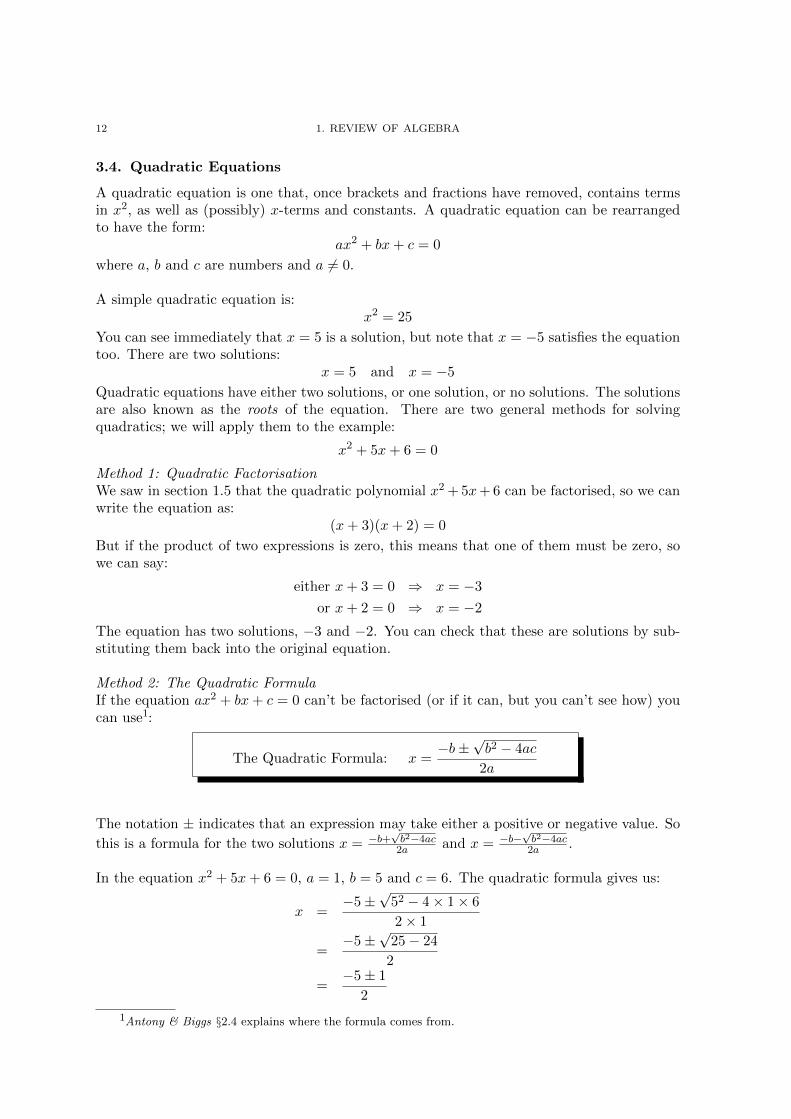
3.4. Quadratic Equations
A quadratic equation is one that, once brackets and fractions have removed, contains termsin x
2, as well as (possibly) x-terms and constants. A quadratic equation can be rearrangedto have the form:
ax
2 + bx+ c = 0
where a, b and c are numbers and a 6= 0.
A simple quadratic equation is:x
2 = 25
You can see immediately that x = 5 is a solution, but note that x = �5 satisfies the equationtoo. There are two solutions:
x = 5 and x = �5
Quadratic equations have either two solutions, or one solution, or no solutions. The solutionsare also known as the roots of the equation. There are two general methods for solvingquadratics; we will apply them to the example:
x
2 + 5x+ 6 = 0
Method 1: Quadratic Factorisation
We saw in section 1.5 that the quadratic polynomial x2 +5x+6 can be factorised, so we canwrite the equation as:
(x+ 3)(x+ 2) = 0
But if the product of two expressions is zero, this means that one of them must be zero, sowe can say:
either x+ 3 = 0 ) x = �3
or x+ 2 = 0 ) x = �2
The equation has two solutions, �3 and �2. You can check that these are solutions by sub-stituting them back into the original equation.
Method 2: The Quadratic Formula
If the equation ax
2 + bx+ c = 0 can’t be factorised (or if it can, but you can’t see how) youcan use1:
The Quadratic Formula: x =�b±
p
b
2� 4ac
2a
The notation ± indicates that an expression may take either a positive or negative value. So
this is a formula for the two solutions x = �b+pb
2�4ac2a and x = �b�
pb
2�4ac2a .
In the equation x
2 + 5x+ 6 = 0, a = 1, b = 5 and c = 6. The quadratic formula gives us:
x =�5±
p
52 � 4⇥ 1⇥ 6
2⇥ 1
=�5±
p
25� 24
2
=�5± 1
2
1Antony & Biggs §2.4 explains where the formula comes from.

1. REVIEW OF ALGEBRA 13
So the two solutions are:
x =�5 + 1
2= �2 and x =
�5� 1
2= �3
Note that in the quadratic formula x = �b±pb
2�4ac2a , b2 � 4ac could turn out to be zero, in
which case there is only one solution. Or it could be negative, in which case there are nosolutions since we can’t take the square root of a negative number.
Examples 3.2: Solve, if possible, the following quadratic equations.
(i) x
2 + 3x� 10 = 0Factorise:
(x+ 5)(x� 2) = 0
) x = �5 or x = 2
(ii) x(7� 2x) = 6First, rearrange the equation to get it into the usual form:
7x� 2x2 = 6
�2x2 + 7x� 6 = 0
2x2 � 7x+ 6 = 0
Now, we can factorise, to obtain:
(2x� 3)(x� 2) = 0
either 2x� 3 = 0 ) x = 32
or x� 2 = 0 ) x = 2
The solutions are x = 32 and x = 2.
(iii) y
2 + 4y + 4 = 0Factorise:
(y + 2)(y + 2) = 0
=) y + 2 = 0 ) y = �2
Therefore y = �2 is the only solution. (Or we sometimes say that the equation has arepeated root – the two solutions are the same.)
(iv) x
2 + x� 1 = 0In section 1.5 we couldn’t find the factors for this example. So apply the formula,putting a = 1, b = 1, c = �1:
x =�1±
p1� (�4)
2=
�1±p
5
2
The two solutions, correct to 3 decimal places, are:
x = �1+p5
2 = 0.618 and x = �1�p5
2 = �1.618
Note that this means that the factors are, approximately, (x� 0.618) and (x+ 1.618).

14 1. REVIEW OF ALGEBRA
(v) 2z2 + 2z + 5 = 0
Applying the formula gives: z =�2±
p
�36
4So there are no solutions, because this contains the square root of a negative number.
(vi) 6x2 + 2kx = 0 (solve for x, treating k as a parameter)Factorising:
2x(3x+ k) = 0
either 2x = 0 ) x = 0
or 3x+ k = 0 ) x = �
k
3
Exercises 1.10: Solve the following quadratic equations, where possible:
(1)(1) x
2 + 3x� 13 = 0
(2) 4y2 + 9 = 12y
(3) 3z2 � 2z � 8 = 0
(4) 7x� 2 = 2x2
(5) y
2 + 3y + 8 = 0
(6) x(2x� 1) = 2(3x� 2)
(7) x
2� 6kx+ 9k2 = 0 (where k is a parameter)
(8) y
2� 2my + 1 = 0 (where m is a parameter)
Are there any values of m for which this equation has no solution?
3.5. Equations involving Indices
Examples 3.3:
(i) 72x+1 = 8Here the variable we want to find, x, appears in a power.This type of equation can by solved by taking logs of both sides:
log10�72x+1
�= log10 (8)
(2x+ 1) log10 7 = log10 8
2x+ 1 =log10 8
log10 7= 1.0686
2x = 0.0686
x = 0.0343
(ii) (2x)0.65 + 1 = 6We can use the rules for indices to manipulate this equation:

1. REVIEW OF ALGEBRA 15
Subtract 1 from both sides: (2x)0.65 = 5
Raise both sides to the power 10.65 :
�(2x)0.65
� 10.65 = 5
10.65
2x = 51
0.65 = 11.894
Divide by 2: x = 5.947
3.6. Equations involving Logarithms
Examples 3.4: Solve the following equations:
(i) log5(3x� 2) = 2From the definition of a logarithm, this equation is equivalent to:
3x� 2 = 52
which can be solved easily:
3x� 2 = 25 ) x = 9
(ii) 10 log10(5x+ 1) = 17
) log10(5x+ 1) = 1.7
5x+ 1 = 101.7 = 50.1187 (correct to 4 decimal places)
x = 9.8237
Exercises 1.11: Solve the following equations:
(1)(1) log4(2 + x) = 2
(2) 16 = 53t
(3) 2 + x
0.4 = 8
The remaining questions are a bit harder – skipthem if you found this section di�cult.
(4) 4.1 + 5x0.42 = 7.8
(5) 6x2�7 = 36
(6) log2(y2 + 4) = 3
(7) 3n+1 = 2n
(8) 2 log10(x� 2) = log10(x)
Further reading and exercises
• For more practice on solving all the types of equation in this section, you could usean A-level pure maths textbook.
• Jacques §1.5 gives more detail on Changing the Subject of a Formula
• Jacques §2.1 and Anthony & Biggs §2.4 both cover the Quadratic Formula for SolvingQuadratic Equations
• Jacques §2.3 has more Equations involving Indices

16 1. REVIEW OF ALGEBRA
↵⌦
� 4. Simultaneous Equations
So far we have looked at equations involving one variable (such as x). An equation involvingtwo variables, x and y, such as x + y = 20, has lots of solutions – there are lots of pairs ofnumbers x and y that satisfy it (for example x = 3 and y = 17, or x = �0.5 and y = 20.5).
But suppose we have two equations and two variables:
x+ y = 20(1)
3x = 2y � 5(2)
There is just one pair of numbers x and y that satisfy both equations.
Solving a pair of simultaneous equations means finding the pair(s) of values that satisfyboth equations. There are two approaches; in both the aim is to eliminate one of the vari-ables, so that you can solve an equation involving one variable only.
Method 1: Substitution
Make one variable the subject of one of the equations (it doesn’t matter which), and substi-tute it in the other equation.
From equation (1): x = 20� y
Substitute for x in equation (2): 3(20� y) = 2y � 5
Solve for y: 60� 3y = 2y � 5�5y = �65
y = 13
From the equation in the first step: x = 20� 13 = 7
The solution is x = 7, y = 13.
Method 2: Elimination
Rearrange the equations so that you can add or subtract them to eliminate one of the vari-ables.
Write the equations as: x+ y = 203x� 2y = �5
Multiply the first one by 2: 2x+ 2y = 403x� 2y = �5
Add the equations together: 5x = 35 ) x = 7
Substitute back in equation (1): 7 + y = 20 ) y = 13
Examples 4.1: Simultaneous Equations
(i) Solve the equations 3x+ 5y = 12 and 2x� 6y = �20
Multiply the first equation by 2 and the second one by 3:

1. REVIEW OF ALGEBRA 17
6x+ 10y = 246x� 18y = -60
Subtract: 28y = 84 ) y = 3Substitute back in the 2nd equation: 2x� 18 = �20 ) x = �1
(ii) Solve the equations x+ y = 3 and x
2 + 2y2 = 18
Here the first equation is linear but the second is quadratic.Use the linear equation for a substitution:
x = 3� y
) (3� y)2 + 2y2 = 18
9� 6y + y
2 + 2y2 = 18
3y2 � 6y � 9 = 0
y
2� 2y � 3 = 0
Solving this quadratic equation gives two solutions for y:
y = 3 or y = �1
Now find the corresponding values of x using the linear equation: when y = 3, x = 0and when y = �1, x = 4. So there are two solutions:
x = 0, y = 3 and x = 4, y = �1
(iii) Solve the equations x+ y + z = 6, y = 2x, and 2y + z = 7
Here we have three equations, and three variables. We use the same methods, toeliminate first one variable, then another.Use the second equation to eliminate y from both of the others:
x+ 2x+ z = 6 ) 3x+ z = 6
4x+ z = 7
Eliminate z by subtracting: x = 1Work out z from 4x+ z = 7: z = 3Work out y from y = 2x: y = 2The solution is x = 1, y = 2, z = 3.
Exercises 1.12: Solve the following sets of simultaneous equations:
(1)(1) 2x = 1� y and 3x+ 4y + 6 = 0
(2) 2z + 3t = �0.5 and 2t� 3z = 10.5
(3) x+ y = a and x = 2y for x and y, in terms of the parameter a.
(4) a = 2b, a+ b+ c = 12 and 2b� c = 13
(5) x� y = 2 and x
2 = 4� 3y2
Further reading and exercises
• Jacques §1.2 covers Simultaneous Linear Equations thoroughly.

18 1. REVIEW OF ALGEBRA
↵⌦
� 5. Inequalities and Absolute Value
5.1. Inequalities
2x+ 1 6
is an example of an inequality. Solving the inequality means “finding the set of values of xthat make the inequality true.” This can be done very similarly to solving an equation:
2x+ 1 6
2x 5
x 2.5
Thus, all values of x less than or equal to 2.5 satisfy the inequality.
When manipulating inequalities you can add anything toboth sides, or subtract anything, and you can multiply ordivide both sides by a positive number. But if you multiplyor divide both sides by a negative number you must reverse
the inequality sign.
To see why you have to reverse the inequality sign, think about the inequality:5 < 8 (which is true)
If you multiply both sides by 2, you get: 10 < 16 (also true)But if you just multiplied both sides by �2, you would get: �10 < �16 (NOT true)Instead we reverse the sign when multiplying by �2, to obtain: �10 > �16 (true)
Examples 5.1: Solve the following inequalities:
(i) 3(x+ 2) > x� 4
3x+ 6 > x� 4
2x > �10
x > �5
(ii) 1� 5y �9
�5y �10
y � 2
5.2. Absolute Value
The absolute value, or modulus, of x is the positive number which has the same “magnitude”as x. It is denoted by |x|. For example, if x = �6, |x| = 6 and if y = 7, |y| = 7.
|x| = x if x � 0|x| = �x if x < 0
Examples 5.2: Solving equations and inequalities involving absolute values
(i) Find the values of x satisfying |x+ 3| = 5.
|x+ 3| = 5 ) x+ 3 = ±5

1. REVIEW OF ALGEBRA 19
Either: x+ 3 = 5 ) x = 2or: x+ 3 = �5 ) x = �8
So there are two solutions: x = 2 and x = �8
(ii) Find the values of y for which |y| 6.
Either: y 6or: �y 6 ) y � �6
So the solution is: �6 y 6
(iii) Find the values of z for which |z � 2| > 4.
Either: z � 2 > 4 ) z > 6or: �(z � 2) > 4 ) z � 2 < �4 ) z < �2
So the solution is: z < �2 or z > 6
5.3. Quadratic Inequalities
Examples 5.3: Solve the inequalities:
(i) x
2� 2x� 15 0
Factorise:(x� 5)(x+ 3) 0
If the product of two factors is negative, one must be negative and the other positive:
either: x� 5 0 and x+ 3 � 0 ) �3 x 5
or: x� 5 � 0 and x+ 3 0 which is impossible.
So the solution is: �3 x 5
(ii) x
2� 7x+ 6 > 0
) (x� 6)(x� 1) > 0
If the product of two factors is positive, both must be positive, or both negative:
either: x� 6 > 0 and x� 1 > 0 which is true if: x > 6
or: x� 6 < 0 and x� 1 < 0 which is true if: x < 1
So the solution is: x < 1 or x > 6
Exercises 1.13: Solve the following equations and inequalities:
(1)(1) (a) 2x+ 1 � 7 (b) 5(3� y) < 2y + 3
(2) (a) |9� 2x| = 11 (b) |1� 2z| > 2
(3) |x+ a| < 2 where a is a parameter, and we know that 0 < a < 2.
(4) (a) x2 � 8x+ 12 < 0 (b) 5x� 2x2 �3
Further reading and exercises
• Jacques §1.4.1 has a little more on Inequalities.• Refer to an A-level pure maths textbook for more detail and practice.

20 1. REVIEW OF ALGEBRA
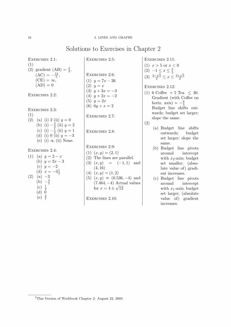
Solutions to Exercises in Chapter 1
Exercises 1.1:
(1) (a) 29(b) �8(c) �15(d) 1
2(e) 64(f) 3
Exercises 1.2:
(1) (a) x
3 + 13x� 25(b) 2x2 � 8y
or 2(x2 � 4y)(2) (a) 3z2x+ 2z � 1
(b) 7x+ 14or 7(x+ 2)
(3) (a) xy
2
(b) 6yx
(4) (a) x
4y
(b) 20x3y4
(5) (a) y
(b) 4x2
y
3
(6) (a) 10x+312
(b) 2x
2�1
Exercises 1.3:
(1) (a) 3x(1 + 2y)(b) y(2y + 7)(c) 3(2a+ b+ 3c)
(2) (a) x
2(3x� 10)(b) c(a� b)
(3) (x+ 2)(y + 2z)(4) x(2� x)
Exercises 1.4:
(1) (x+ 1)(x+ 3)(2) (y � 5)(y � 2)(3) (2x+ 1)(x+ 3)(4) (z + 5)(z � 3)(5) (2x+ 3)(2x� 3)(6) (y � 5)2
(7) Not possible to split intointeger factors.
Exercises 1.5:
(1) (a) =p
2⇥ 18=
p
36 = 6(b) =
p
49⇥ 5= 7
p
5(c) 15p
3= 15
p3
3
= 5p
3(2) (a)
p
5(b) 4x2
(c) x
2
(d)p
2y
Exercises 1.6:
(1) (a) 16(b) 6(c) 3(d) 1
4
(2) (a) 2x11
(b) 1x
(c) log10 y(d) 3
(3) (a) (9ab)3
(b) �
53 log10 b
Exercises 1.7:
(1) x = 3(2) y = �3(3) x = 2(4) z = �1(5) a = �
13
Exercises 1.8:
(1) x = 6a
(2) y = �4b(3) z = a+b
2
Exercises 1.9:
(1) t = v�u
a
(2) a =p
c
2� b
2
(3) p = 1200r � 6n(4) n = W
m
2 + 3
Exercises 1.10:
(1) x = �3±p61
2(2) y = 1.5(3) z = �
43 , 2
(4) x = 7±p33
4(5) No solutions.
(6) x = 7±p17
4(7) x = 3k(8) y = (m±
p
m
2� 1)
No solution if�1 < m < 1
Exercises 1.11:
(1) x = 14
(2) t = log(16)3 log(5) = 0.5742
(3) x = 610.4 = 88.18
(4) x = (0.74)1
0.42 = 0.4883(5) x = ±3(6) y = ±2
(7) n = log2 3
log223
= �2.7095
(8) x = 4, x = 1
Exercises 1.12:
(1) x = 2, y = �3(2) t = 1.5, z = �2.5(3) x = 2a
3 , y = a
3(4) a = 10, b = 5,
c = �3(5) (x, y) = (2, 0)
(x, y) = (1,�1)
Exercises 1.13:
(1) (a) x � 3(b) 12
7 < y
(2) (a) x = �1, 10(b) z < �0.5 or z > 1.5
(3) �2� a < x < 2� a
(4) (a) 2 < x < 6(b) x � 3, x �0.5
2This Version of Workbook Chapter 1: September 25, 2014

1. REVIEW OF ALGEBRA 21
⌥⌃ ⌅⇧Worksheet 1: Review of Algebra
(1) For a firm, the cost of producing q units of output is C = 4 + 2q + 0.5q2. What isthe cost of producing (a) 4 units (b) 1 unit (c) no units?
(2) Evaluate the expression x
3(y + 7) when x = �2 and y = �10.
(3) Simplify the following algebraic expressions, factorising the answer where possible:
(a) x(2y+3x�12)�3(2�5xy)� (3x+8xy�6) (b) z(2�3z+5z2)+3(z2�z
3�4)
(4) Simplify: (a) 6a4b⇥ 4b÷ 8ab3c (b)p
3x3y ÷p
27xy (c) (2x3)3 ⇥ (xz2)4
(5) Write as a single fraction: (a)2y
3x+
4y
5x(b)
x+ 1
4�
2x� 1
3
(6) Factorise the following quadratic expressions:(a) x2 � 7x+ 12 (b) 16y2 � 25 (c) 3z2 � 10z � 8
(7) Evaluate (without using a calculator): (a) 432 (b) log10 100 (c) log5 125
(8) Write as a single logarithm: (a) 2 loga
(3x) + loga
x
2 (b) loga
y � 3 loga
z
(9) Solve the following equations:
(a) 5(2x� 9) = 2(5� 3x) (b) 1 +6
y � 8= �1 (c) z0.4 = 7 (d) 32t�1 = 4
(10) Solve these equations for x, in terms of the parameter a:
(a) ax� 7a = 1 (b) 5x� a =x
a
(c) loga
(2x+ 5) = 2
(11) Make Q the subject of: P =
ra
Q
2 + b
(12) Solve the equations: (a) 7� 2x2 = 5x (b) y2 + 3y � 0.5 = 0 (c) |1� z| = 5
(13) Solve the simultaneous equations:(a) 2x� y = 4 and 5x = 4y + 13(b) y = x
2 + 1 and 2y = 3x+ 4
(14) Solve the inequalities: (a) 2y � 7 3 (b) 3� z > 4 + 2z (c) 3x2 < 5x+ 2

CHAPTER 2
Lines and Graphs
Almost everything in this chapter is revision from GCSE maths. It re-minds you how to draw graphs, and focuses in particular on straightline graphs and their gradients. We also look at graphs of quadraticfunctions, and use graphs to solve equations and inequalities. An im-portant economic application of straight line graphs is budget con-straints.
—./—⌥⌃
⌅⇧1. The Gradient of a Line
A is a point with co-ordinates (2, 1); B has co-ordinates (6, 4).
.
...............................................................................................................................................................................................................................................................................................................................................
x
y
1 2 3 4 5 6-1
1
2
3
4
5
-1
A
B
4
3
When you move from A to B, thechange in the x-coordinate is
�x = 6� 2 = 4
and the change in the y-coordinateis
�y = 4� 1 = 3The gradient (or slope) of AB is �y
divided by �x:
Gradient =�y
�x
=34
= 0.75
(The symbol �, pronounced “delta”, denotes “change in”.)
It doesn’t matter which end of the line you start. If you move from B to A, the changesare negative, but the gradient is the same: �x = 2 � 6 = �4 and �y = 1 � 4 = �3, so thegradient is (�3)/(�4) = 0.75.
There is a general formula:
The gradient of the line joining (x1, y1) and (x2, y2) is:�y
�x
=y2 � y1
x2 � x1
23

24 2. LINES AND GRAPHS
.
.........................................................................................................................................................................................................................................................................................................................
x
y
1 2 3 4 5 6-1
1
2
3
4
5
-1
C
D
2
4
Here the gradient is negative. Whenyou move from C to D:
�x = 4� 2 = 2
�y = 1� 5 = �4The gradient of CD is:
�y
�x
=�42
= �2
.
....................................................................................................................................................................................................
.
....................................
....................................
....................................
....................................
..........
x
y
a
b
c
d
In this diagram the gradient of line a is positive,and the gradient of b is negative: as you movein the x-direction, a goes uphill, but b goesdownhill.
The gradient of c is zero. As you movealong the line the change in the y-coordinate iszero: �y = 0
The gradient of d is infinite. As you movealong the line the change in the x-coordinate iszero (so if you tried to calculate the gradientyou would be dividing by zero).
Exercises 2.1: Gradients(1)(1) Plot the points A(1, 2), B(7, 10), C(�4, 14), D(9, 2) and E(�4,�1) on a diagram.
(2) Find the gradients of the lines AB,AC,CE, AD.

2. LINES AND GRAPHS 25
↵⌦
� 2. Drawing Graphs
The equation y = 0.5x+1 expresses a relationship between 2 quantities x and y (or a formulafor y in terms of x) that can be represented as a graph in x-y space. To draw the graph,calculate y for a range of values of x, then plot the points and join them with a curve or line.
Examples 2.1: y = 0.5x + 1
.
....................................................................................................................................................................................................................................................................................................................................................................................................................................................................................................................................................................................................................................................................................................................................................................................................................................................................................................................................................................................................................................
..............
...........
.......................
..............
...........
.......................
..............
...........
.......................
x
y
�4�1
01
43
(�4,�1)
(0, 1)
(4, 3)
x
y
Examples 2.2: y = 0.5x
2� x� 4
.
...................................................
................................................
.............................................
..........................................
........................
...............
..........................
..........
..........................
.......
............................
...
..............................
.............................
............................
........................... .......................... ......................... ........................ ......................... .....................................................
............................
.............................
..............................
...............................
.................................
....................................
.......................................
..........................................
.............................................
................................................
...................................................
x
y
�3
3.5
�1
�2.5
0
�4
1
�4.5
3
�2.5
5
3.5
(�3, 3.5)
(0,�4)
(5, 3.5)
x
y
Exercises 2.2: Draw the graphs of the following relationships:(1)(1) y = 3x� 2 for values of x between �4 and +4.
(2) P = 10�2Q, for values of Q between 0 and 5. (This represents a demand function:the relationship between the market price P and the total quantity sold Q.)
(3) y = 4/x, for values of x between �4 and +4.
(4) C = 3+2q2, for values of q between 0 and 4. (This represents a firm’s cost function:its total costs are C if it produces a quantity q of goods.)

26 2. LINES AND GRAPHS
↵⌦
� 3. Straight Line (Linear) Graphs
Exercises 2.3: Straight Line Graphs(1)(1) Using a diagram with x and y axes from �4 to +4, draw the graphs of:
(a) y = 2x
(b) 2x + 3y = 6
(c) y = 1� 0.5x
(d) y = �3
(e) x = 4
(2) For each graph find (i) the gradient, and (ii) the vertical intercept (that is, thevalue of y where the line crosses the y-axis, also known as the y-intercept).
Each of the first four equations in this exercise can be rearranged to have the form y = mx+c:
(a) y = 2x ) y = 2x + 0 ) m = 2 c = 0(b) 2x + 3y = 6 ) y = �2
3x + 2 ) m = �23 c = 2
(c) y = 1� 0.5x ) y = �0.5x + 1 ) m = �0.5 c = 1(d) y = �3 ) y = 0x� 3 ) m = 0 c = �3
(e) is a special case. It cannot be written in the form y = mx + c, its gradient is infinite, andit has no vertical intercept.
Check these values of m and c against your answers. You should find that m is the gra-dient and c is the y-intercept.
Note that in an equation of the form y = mx + c, y is equal to a polynomial of degree1 in x (see Chapter 1).
.
...................................................................................................................................................................................................................................................................................................................................................................................................................................................................................................................................................
y = mx + c
�x
�y
�y
�x
= m
(0, c)
y
x
If an equation can be written in the form y = mx + c, thenthe graph is a straight line, with gradient m and vertical
intercept c. We say “y is a linear function of x.”

2. LINES AND GRAPHS 27
Examples 3.1: Sketch the line x� 2y = 2
“Sketching” a graph meansdrawing a picture to indicateits general shape and position,rather than plotting it accu-rately. First rearrange theequation:
y = 0.5x� 1
So the gradient is 0.5 and they-intercept is �1. We can usethis to sketch the graph.
.
............................................................................................................................................................................................................................................................................................................................................................................................................................................................................................................................................................................................................................................................................................................
x
y
(2, 0)
(0,�1)
Exercises 2.4: y = mx + c
(1)(1) For each of the lines in the diagram below, work out the gradient and hence writedown the equation of the line.
(2) By writing each of the following lines in the form y = mx + c, find its gradient:(a) y = 4� 3x (b) 3x + 5y = 8 (c) x + 5 = 2y (d) y = 7 (e) 2x = 7y
(3) By finding the gradient and y-intercept, sketch each of the following straight lines:y = 3x + 5y + x = 63y + 9x = 8x = 4y + 3
.
..........................
..........................
..........................
..........................
..........................
..........................
..........................
..........................
..........................
..........................
..........................
..........................
..........................
..........................
..........................
..........................
..........................
..........................
..........................
..........................
..........................
..........................
..........................
..........................
..........................
..........................
..........................
..........................
..........................
..........................
..........................
..........................
..........................
..........................
.........
.
..............................................................................................................................................................................................................................................................................................................................................................................................................................................................................................................................................................................................................................................................................................................................................................................................................
3
-3
6-6
d
c
a
b
x
y

28 2. LINES AND GRAPHS
3.1. Lines of the Form ax + by = c
Lines such as 2x+3y = 6 can be rearranged to have the form y = mx+c, and hence sketched,as in the previous exercise. But it is easier in this case to work out what the line is like byfinding the points where it crosses both axes.
Examples 3.2:Sketch the line 2x + 3y = 6.
When x = 0, y = 2When y = 0, x = 3
.
................................
................................
................................
................................
................................
................................
................................
................................
................................
................................
................................
................................
................................
................................
................................
................................
................................
................
x
y
(3, 0)
(0, 2)
Exercises 2.5: Sketch the following lines: (1) 4x + 5y = 100 (2) 2y + 6x = 7
3.2. Working out the Equation of a Line
Examples 3.3: What is the equation of the line
(i) with gradient 3, passing through (2, 1)?gradient = 3 ) y = 3x + c
y = 1 when x = 2 ) 1 = 6 + c ) c = �5The line is y = 3x� 5.
(ii) passing through (�1,�1) and (5, 14)?First work out the gradient: 14�(�1)
5�(�1) = 156 = 2.5
gradient = 2.5 ) y = 2.5x + c
y = 14 when x = 5 ) 14 = 12.5 + c) c = 1.5The line is y = 2.5x + 1.5 (or equivalently 2y = 5x + 3).
There is a formula that you can use (although the method above is just as good):
The equation of a line with gradient m, passing throughthe point (x1, y1) is: y = m(x� x1) + y1
Exercises 2.6: Find the equations of the following lines:(1)(1) passing through (4, 2) with gradient 7
(2) passing through (0, 0) with gradient 1
(3) passing through (�1, 0) with gradient �3
(4) passing through (�3, 4) and parallel to the line y + 2x = 5
(5) passing through (0, 0) and (5, 10)
(6) passing through (2, 0) and (8,�1)

2. LINES AND GRAPHS 29
↵⌦
� 4. Quadratic Graphs
If we can write a relationship between x and y so that y is equal to a quadratic polynomialin x (see Chapter 1):
y = ax
2 + bx + c
where a, b and c are numbers, then we say “y is a quadratic function of x”, and the graph isa parabola (a U-shape) like the one in Example 2.2.
Exercises 2.7: Quadratic Graphs(1)(1) Draw the graphs of (i) y = 2x
2� 5 (ii) y = �x
2 + 2x, for values of x between �3and +3.
(2) For each graph note that: if a (the coe�cient of x
2) is positive, the graph is aU-shape; if a is negative then it is an inverted U-shape; the vertical intercept isgiven by c; and the graph is symmetric.
So, to sketch the graph of a quadratic you can:• decide whether it is a U-shape or an inverted U;• find the y-intercept;• find the points where it crosses the x-axis (if any), by solving ax
2 + bx + c = 0;• find its maximum or minimum point using symmetry: find two points with the same
y-value, then the max or min is at the x-value halfway between them.
Examples 4.1: Sketch the graph of y = �x
2� 4x
• a = �1, so it is an inverted U-shape.• The y-intercept is 0.• Solving �x
2� 4x = 0 to find where it crosses
the x-axis:
x
2 + 4x = 0 ) x(x + 4) = 0) x = 0 or x = �4
• Its maximum point is halfway between thesetwo points, at x = �2, and at this pointy = �4� 4(�2) = 4. .
..........................................
.......................................
....................................
.................................
..............................
...........................
........................
.....................
.................................................................. .............. .............. ............... ................
.................
..................
.....................
........................
...........................
..............................
.................................
....................................
.......................................
..........................................
(�2, 4)
(�4, 0)x
y
Exercises 2.8: Sketch the graphs of the following quadratic functions:(1)(1) y = 2x
2� 18
(2) y = 4x� x
2 + 5

30 2. LINES AND GRAPHS
✏�
��
5. Solving Equations and Inequalities
using Graphs
5.1. Solving Simultaneous Equations
The equations:
x + y = 4y = 3x
could be solved algebraically(see Chapter 1). Alterna-tively we could draw theirgraphs, and find the pointwhere they intersect.
The solution is x = 1, y = 3.
.
..........................
..........................
..........................
..........................
..........................
..........................
..........................
..........................
..........................
..........................
..........................
..........................
..........................
..........................
..........................
..........................
..........................
..........................
..........................
..........................
..........................
............
.
...............................................................................................................................................................................................................................................................................................................................................................................................................................................................
x
y
x + y = 4
y = 3x
(1, 3)
5.2. Solving Quadratic Equations
We could solve the solve the quadratic equation x
2� 5x + 2 = 0 using the quadratic formula
(see Chapter 1). Alternatively we could find an approximate solution by drawing the graphof y = x
2� 5x + 2 (as accurately as possible), and finding where it crosses the x-axis (that
is, finding the points where y = 0).
Exercises 2.9: Solving Equations using Graphs(1)(1) Solve the simultaneous equations y = 4x�7 and y = x�1 by drawing (accurately)
the graphs of the two lines.
(2) By sketching their graphs, explain why you cannot solve either of the followingpairs of simultaneous equations:
y = 3x� 5 and 2y � 6x = 7;x� 5y = 4 and y = 0.2x� 0.8
(3) By sketching their graphs, show that the simultaneous equations y = x
2 andy = 3x + 4 have two solutions. Find the solutions algebraically.
(4) Show algebraically that the simultaneous equations y = x
2 + 1 and y = 2x haveonly one solution. Draw the graph of y = x
2 + 1 and use it to show that thesimultaneous equations:
y = x
2 + 1 and y = mx
have: no solutions if 0 < m < 2; one solution if m = 2; and two solutions if m > 2.
(5) Sketch the graph of the quadratic function y = x
2� 8x. From your sketch, find
the approximate solutions to the equation x
2� 8x = �4.

2. LINES AND GRAPHS 31
5.3. Representing Inequalities using Graphs
If we draw the graph of theline 2y+x = 10, all the pointssatisfying 2y + x < 10 lie onone side of the line. The dot-ted region shows the inequal-ity 2y + x < 10.
.
........................................
........................................
........................................
........................................
........................................
........................................
........................................
........................................
........................................
........................................
........................................
........................................
........................................
........................................
........................................
........................................
........................................
........................................
...........................
. .
. . . .
. . . . . .
. . . . . . .
. . . . . . . . .
. . . . . . . . . . .
. . . . . . . . . . . .
. . . . . . . . . . . . . .
. . . . . . . . . . . . . . . .
. . . . . . . . . . . . . . . .
(0, 5)
(10, 0)x
y
Exercises 2.10: Representing Inequalities(1)(1) Draw a sketch showing all the points where x + y < 1 and y < x + 1 and y > �3.
(2) Sketch the graph of y = 3� 2x
2, and show the region where y < 3� 2x
2.
5.4. Using Graphs to Help Solve Quadratic Inequalities
In Chapter 1, we solved quadratic inequalities such as: x
2� 2x � 15 0. To help do this
quickly, you can sketch the graph of the quadratic polynomial y = x
2� 2x� 15.
Examples 5.1: Quadratic Inequalities
(i) Solve the inequality x
2� 2x� 15 0.
As before, the first step is to factorise:
(x� 5)(x + 3) 0
Now sketch the graph of y = x
2�2x�15.
We can see from the graph that x
2� 2x�
15 0 when:
�3 x 5
This is the solution of the inequality.
(ii) Solve the inequality x
2� 2x� 15 > 0.
From the same graph the solution is: x >
5 or x < �3.
.
.....................................................
..................................................
...............................................
............................................
.........................................
.....................................
..................................
...............................
............................
.........................
......................
...................
.................
................ ............... .............. .............. ................................................
...................
......................
.........................
............................
...............................
..................................
.....................................
.........................................
............................................
...............................................
..................................................
.....................................................
(�3, 0) (5, 0)x
y
Exercises 2.11: Solve the inequalities:(1)(1) x
2� 5x > 0
(2) 3x + 5� 2x
2� 0
(3) x
2�3x+1 0 (Hint: you will need to use the quadratic formula for the last one.)

32 2. LINES AND GRAPHS
✏�
��
6. Economic Application: Budget
Constraints
6.1. An Example
Suppose pencils cost 20p, and pens cost 50p. If a student buys x pencils and y pens, thetotal amount spent is:
20x + 50y
If the maximum amount he has to spend on writing implements is £5 his budget constraintis:
20x + 50y 500
His budget set (the choices of pens andpencils that he can a↵ord) can be shownas the shaded area on a diagram:
From the equation of the budget line:
20x + 50y = 500
we can see that the gradient of the budgetline is:
�
2050
(You could rewrite the equation in theform y = mx + c.)
.
............................................................................................................................................................................................................................................................................................................................................................................................................................................................................................
.
.
.
.
.
.
.
.
.
.
.
.
.
.
.
.
.
.
.
.
.
.
.
.
.
.
.
.
.
.
.
.
.
.
..
.
.
.
.
.
.
.
.
.
.
.
.
.
.
.
.
.
.
.
.
.
.
.
.
.
.
.
.
.
.
.
.
.
.
.
.
.
.
.
.
.
.
.
.
.
.
.
.
.
.
.
.
.
.
.
.
.
.
.
.
.
.
.
.
.
.
.
.
.
.
.
.
.
.
.
.
.
.
. . .
x
y
25
10
6.2. The General Case
Suppose that a consumer has a choice of two goods, good 1 and good 2. The price of good 1is p1 and the price of good 2 is p2. If he buys x1 units of good 1, and x2 units of good 2, thetotal amount spent is:
p1x1 + p2x2
If the maximum amount he has to spend is his income I his budget constraint is:
p1x1 + p2x2 I
To draw the budget line:
p1x1 + p2x2 = I
note that it crosses the x1-axis where:
x2 = 0) p1x1 = I ) x1 =I
p1
and similarly for the x2 axis.
The gradient of the budget line is:
�
p1
p2
.
.............................................................................................................................................................................................................................................................................................................................................................................................................................................. x1
x2
I
p1
I
p2

2. LINES AND GRAPHS 33
Exercises 2.12: Budget Constraints(1)(1) Suppose that the price of co↵ee is 30p and the price of tea is 25p. If a consumer
has a daily budget of £1.50 for drinks, draw his budget set and find the slope ofthe budget line. What happens to his budget set and the slope of the budget lineif his drinks budget increases to £2?
(2) A consumer has budget constraint p1x1 + p2x2 I. Show diagrammatically whathappens to the budget set if
(a) income I increases
(b) the price of good 1, p1, increases
(c) the price of good 2, p2, decreases.
Further reading and exercises• Jacques §1.1 has more on co-ordinates and straight-line graphs.• Jacques §2.1 includes graphs of quadratic functions.• Varian discusses budget constraints in detail.
34 2. LINES AND GRAPHS
Solutions to Exercises in Chapter 2
Exercises 2.1:(1)(2) gradient (AB) = 4
3 ,(AC) = �12
5 ,(CE) = 1,(AD) = 0
Exercises 2.2:
Exercises 2.3:(1)(2) (a) (i) 2 (ii) y = 0
(b) (i) �23 (ii) y = 2
(c) (i) �12 (ii) y = 1
(d) (i) 0 (ii) y = �3(e) (i) 1 (ii) None.
Exercises 2.4:(1) (a) y = 2� x
(b) y = 2x� 3(c) y = �2(d) x = �31
2(2) (a) �3
(b) �35
(c) 12
(d) 0(e) 2
7
Exercises 2.5:
Exercises 2.6:(1) y = 7x� 26(2) y = x
(3) y + 3x = �3(4) y + 2x = �2(5) y = 2x
(6) 6y + x = 2
Exercises 2.7:
Exercises 2.8:
Exercises 2.9:(1) (x, y) = (2, 1)(2) The lines are parallel.(3) (x, y) = (�1, 1) and
(4, 16)(4) (x, y) = (1, 2)(5) (x, y) ⇡ (0.536,�4) and
(7.464,�4) Actual valuesfor x = 4±
p
12
Exercises 2.10:
Exercises 2.11:(1) x > 5 or x < 0(2) �1 x
52
(3) 3�p
52 x
3+p
52
Exercises 2.12:(1) 6 Co↵ee + 5 Tea 30.
Gradient (with Co↵ee onhoriz. axis) = �6
5Budget line shifts out-wards; budget set larger;slope the same.
(2)(a) Budget line shifts
outwards; budgetset larger; slope thesame.
(b) Budget line pivotsaround interceptwith x2-axis; budgetset smaller; (abso-lute value of) gradi-ent increases.
(c) Budget line pivotsaround interceptwith x1-axis; budgetset larger; (absolutevalue of) gradientincreases.
1This Version of Workbook Chapter 2: August 22, 2003

2. LINES AND GRAPHS 35
⌥⌃ ⌅⇧Worksheet 2: Lines and Graphs
(1) Find the gradients of the lines AB, BC, and CA where A is the point (5, 7), B is(�4, 1) and C is (5,�17).
(2) Draw (accurately), for values of x between �5 and 5, the graphs of:(a) y � 2.5x = �5 (b) z = 1
4x
2 + 12x� 1
Use (b) to solve the equation 14x
2 + 12x = 1
(3) Find the gradient and y-intercept of the following lines:(a) 3y = 7x� 2 (b) 2x + 3y = 12 (c) y = �x
(4) Sketch the graphs of 2P = Q+5, 3Q+4P = 12, and P = 4, with Q on the horizontalaxis.
(5) What is the equation of the line through (1, 1) and (4,�5)?
(6) Sketch the graph of y = 3x� x
2 + 4, and hence solve the inequality 3x� x
2< �4.
(7) Draw a diagram to represent the inequality 3x� 2y < 6.
(8) Electricity costs 8p per unit during the daytime and 2p per unit if used at night. Thequarterly charge is £10. A consumer has £50 to spend on electricity for the quarter.
(a) What is his budget constraint?(b) Draw his budget set (with daytime units as “good 1” on the horizontal axis).(c) Is the bundle (440, 250) in his budget set?(d) What is the gradient of the budget line?
(9) A consumer has a choice of two goods, good 1 and good 2. The price of good 2 is 1,and the price of good 1 is p. The consumer has income M .
(a) What is the budget constraint?(b) Sketch the budget set, with good 1 on the horizontal axis, assuming that p > 1.(c) What is the gradient of the budget line?(d) If the consumer decides to spend all his income, and buy equal amounts of the
two goods, how much of each will he buy?(e) Show on your diagram what happens to the budget set if the price of good 1
falls by 50%.

CHAPTER 3
Sequences, Series, and Limits; the Economics of Finance
If you have done A-level maths you will have studied Sequences andSeries (in particular Arithmetic and Geometric ones) before; if notyou will need to work carefully through the first two sections of thischapter. Sequences and series arise in many economic applications, suchas the economics of finance and investment. Also, they help you tounderstand the concept of a limit and the significance of the natural
number, e. You will need both of these later.
—./—
↵⌦
� 1. Sequences and Series
1.1. Sequences
A sequence is a set of terms (or numbers) arranged in a definite order.
Examples 1.1: Sequences
(i) 3, 7, 11, 15, . . .In this sequence each term is obtained by adding 4 to the previous term. So the nextterm would be 19.
(ii) 4, 9, 16, 25, . . .This sequence can be rewritten as 22, 32, 42, 52, . . . The next term is 62, or 36.
The dots(. . . ) indicate that the sequence continues indefinitely – it is an infinite sequence.A sequence such as 3, 6, 9, 12 (stopping after a finite number of terms) is a finite sequence.Suppose we write u1 for the first term of a sequence, u2 for the second and so on. There maybe a formula for u
n
, the n
th term:
Examples 1.2: The n
th term of a sequence
(i) 4, 9, 16, 25, . . . The formula for the n
th term is un
= (n+ 1)2.
(ii) u
n
= 2n+ 3. The sequence given by this formula is: 5, 7, 9, 11, . . .
(iii) u
n
= 2n + n. The sequence is: 3, 6, 11, 20, . . .
Or there may be a formula that enables you to work out the terms of a sequence from thepreceding one(s), called a recurrence relation:
Examples 1.3: Recurrence Relations
(i) Suppose we know that: un
= u
n�1 + 7n and u1 = 1.Then we can work out that u2 = 1 + 7 ⇥ 2 = 15, u3 = 15 + 7 ⇥ 3 = 36, and so on, tofind the whole sequence : 1, 15, 36, 64, . . .
37

38 3. SEQUENCES, SERIES AND LIMITS
(ii) u
n
= u
n�1 + u
n�2, u1 = 1, u2 = 1The sequence defined by this formula is: 1, 1, 2, 3, 5, 8, 13, . . .
1.2. Series
A series is formed when the terms of a sequence are added together. The Greek letter ⌃(pronounced “sigma”) is used to denote “the sum of”:
nX
r=1
u
r
means u1 + u2 + · · ·+ u
n
Examples 1.4: Series
(i) In the sequence 3, 6, 9, 12, . . . , the sum of the first five terms is the series:3 + 6 + 9 + 12 + 15.
(ii)6X
r=1
(2r + 3) = 5 + 7 + 9 + 11 + 13 + 15
(iii)kX
r=5
1
r
2=
1
25+
1
36+
1
49+ · · ·+
1
k
2
Exercises 3.1: Sequences and Series
(1)(1) Find the next term in each of the following sequences:
(a) 2, 5, 8, 11, . . .
(b) 0.25, 0.75, 1.25, 1.75, 2.25, . . .
(c) 5,�1,�7, . . .
(d) 36, 18, 9, 4.5, . . .
(e) 1,�2, 3,�4, 5, . . .
(2) Find the 2nd, 4th and 6th terms in the sequence given by: un
= n
2� 10
(3) If un
= un�1
2 + 2 and u1 = 4 write down the first five terms of the sequence.
(4) If un
= u
2n�1 + 3u
n�1 and u3 = �2, find the value of u4.
(5) Find the value ofP4
r=1 3r
(6) Write out the following sums without using sigma notation:
(a)P5
r=11r
2 (b)P3
i=0 2i (c)
Pn
j=0(2j + 1)
(7) In the seriesP
n�1i=0 (4i+1), (a) how many terms are there? (b) what is the formula
for the last term?
(8) Express using the ⌃ notation:
(a) 12 + 22 + 32 + ...+ 252 (c) 16 + 25 + 36 + 49 + · · ·+ n
2
(b) 6 + 9 + 12 + · · ·+ 21
Further reading and exercises
• For more practice with simple sequences and series, you could use an A-level puremaths textbook.

3. SEQUENCES, SERIES AND LIMITS 39
✏�
��
2. Arithmetic and Geometric
Sequences
2.1. Arithmetic Sequences
An arithmetic sequence is one in which each term can be obtained by adding a fixed number(called the common di↵erence) to the previous term.
Examples 2.1: Some Arithmetic Sequences
(i) 1, 3, 5, 7, . . . The common di↵erence is 2.
(ii) 13, 7, 1,�5, . . . The common di↵erence is �6.
In an arithmetic sequence with first term a and commondi↵erence d, the formula for the n
thterm is:u
n
= a+ (n� 1)d
Examples 2.2: Arithmetic Sequences
(i) What is the 10th term of the arithmetic sequence 5, 12, 19, . . . ?In this sequence a = 5 and d = 7. So the 10th term is: 5 + 9⇥ 7 = 68.
(ii) If an arithmetic sequence has u10 = 24 and u11 = 27, what is the first term?The common di↵erence, d, is 3. Using the formula for the 11th term:
27 = a+ 10⇥ 3
Hence the first term, a, is �3.
2.2. Arithmetic Series
When the terms in an arithmetic sequence are summed, we obtain an arithmetic series.Suppose we want to find the sum of the first 5 terms of the arithmetic sequence with firstterm 3 and common di↵erence 4. We can calculate it directly:
S5 = 3 + 7 + 11 + 15 + 19 = 55
But there is a general formula:
If an arithmetic sequence has first term a and commondi↵erence d, the sum of the first n terms is:
S
n
=n
2(2a+ (n� 1)d)
We can check that the formula works: S5 =52 (2⇥ 3 + 4⇥ 4) = 55
2.3. To Prove the Formula for an Arithmetic Series
Write down the series in order and in reverse order, then add them together, pairing terms:
S
n
= a + (a+ d) + (a+ 2d) + · · ·+ (a+ (n� 1)d)S
n
= (a+ (n� 1)d) + (a+ (n� 2)d) + (a+ (n� 3)d) + · · ·+ a
2Sn
= (2a+ (n� 1)d) + (2a+ (n� 1)d) + (2a+ (n� 1)d) + · · ·+ (2a+ (n� 1)d)= n (2a+ (n� 1)d)
Dividing by 2 gives the formula.

40 3. SEQUENCES, SERIES AND LIMITS
Exercises 3.2: Arithmetic Sequences and Series
(1)(1) Using the notation above, find the values of a and d for the arithmetic sequences:(a) 4, 7, 10, 13, . . . (b) �1, 2, 5, . . . (c) �7,�8.5,�10,�11.5, . . .
(2) Find the n
th term in the following arithmetic sequences:(a) 44, 46, 48, . . . (b) �3,�7,�11,�15, . . .
(3) If an arithmetic sequence has u20 = 100, and u22 = 108, what is the first term?
(4) Use the formula for an arithmetic series to calculate the sum of the first 8 termsof the arithmetic sequence with first term 1 and common di↵erence 10.
(5) (a) Find the values of a and d for the arithmetic sequence: 21, 19, 17, 15, 13, . . .
(b) Use the formula for an arithmetic series to calculate 21 + 19 + 17 + 15 + 13.
(c) Now use the formula to calculate the sum of 21+19+17+. . . +1.
(6) Is the sequence u
n
= �4n+ 2 arithmetic? If so, what is the common di↵erence?
2.4. Geometric Sequences
A geometric sequence is one in which each term can be obtained by multiplying the previousterm by a fixed number, called the common ratio.
Examples 2.3: Geometric Sequences
(i) 12 , 1, 2, 4, 8, . . . Each term is double the previous one. The common ratio is 2.
(ii) 81, 27, 9, 3, 1, . . . The common ratio is 13 .
In a geometric sequence with first term a and commonratio r, the formula for the n
th term is:u
n
= ar
n�1
Examples 2.4: Consider the geometric sequence with first term 2 and common ratio 1.1.
(i) What is the 10th term?Applying the formula, with a = 2 and r = 1.1, u10 = 2⇥ (1.1)9 = 4.7159
(ii) Which terms of the sequence are greater than 20?The n
th term is given by u
n
= 2⇥ (1.1)n�1. It exceeds 20 if:
2⇥ (1.1)n�1> 20
(1.1)n�1> 10
Taking logs of both sides (see chapter 1, section 5):
log10(1.1)n�1
> log10 10
(n� 1) log10 1.1 > 1
n >
1
log10 1.1+ 1 = 25.2
So all terms from the 26th onwards are greater than 20.

3. SEQUENCES, SERIES AND LIMITS 41
2.5. Geometric Series
Suppose we want to find the sum of the first 10 terms of the geometric sequence with firstterm 3 and common ratio 0.5:
S10 = 3 + 1.5 + 0.75 + · · ·+ 3⇥ (0.5)9
There is a general formula:
For a geometric sequence with first term a and commonratio r, the sum of the first n terms is:
S
n
=a(1� r
n)
1� r
So the answer is: S50 =3(1� (0.5)10)
1� 0.5= 5.994
2.6. To Prove the Formula for a Geometric Series
Write down the series and then multiply it by r:
S
n
= a + ar + ar
2 + ar
3 + . . . + ar
n�1
rS
n
= ar + ar
2 + ar
3 + . . . + ar
n�1 + ar
n
Subtract the second equation from the first:
S
n
� rS
n
= a� ar
n
=) S
n
=a(1� r
n)
1� r
Exercises 3.3: Geometric Sequences and Series
(1)(1) Find the 8th term and the n
th term in the geometric sequence: 5, 10, 20, 40, . . .
(2) Find the 15th term and the n
th term in the geometric sequence: �2, 4,�8, 16, . . .
(3) In the sequence 1, 3, 9, 27, . . . , which is the first term term greater than 1000?
(4) (a) Using the notation above, what are the values of a and r for the sequence:4, 2, 1, 0.5, 0.25, . . . ?
(b) Use the formula for a geometric series to calculate: 4 + 2 + 1 + 0.5 + 0.25.
(5) Find the sum of the first 10 terms of the geometric sequence: 4, 16, 64, . . .
(6) Find the sum of the first n terms of the geometric sequence: 20, 4, 0.8, . . . Simplifyyour answer as much as possible.
(7) Use the formula for a geometric series to show that: 1 +x
2+
x
2
4+
x
3
8=
16� x
4
16� 8x
Further reading and exercises
• For more practice with arithmetic and geometric sequences and series, you could usean A-level pure maths textbook.
• Jacques §3.3 Geometric Series.
42 3. SEQUENCES, SERIES AND LIMITS
✏�
��
3. Economic Application: Interest
Rates, Savings and Loans
Suppose that you invest £500 at the bank, at a fixed interest rate of 6% (that is, 0.06) perannum, and the interest is paid at the end of each year. At the end of one year you receivean interest payment of 0.06⇥ 500 = £30, which is added to your account, so you have £530.After two years, you receive an interest payment of 0.06 ⇥ 530 = £31.80, so that you have£561.80 in total, and so on.1
More generally, if you invest an amount P (the “principal”) and interest is paid annuallyat interest rate i, then after one year you have a total amount y1:
y1 = P (1 + i)
after two years:y2 = (P (1 + i)) (1 + i) = P (1 + i)2
and after t years:y
t
= P (1 + i)t
This is a geometric sequence with common ratio (1 + i).
Examples 3.1: If you save £500 at a fixed interest rate of 6% paid annually:
(i) How much will you have after 10 years?Using the formula above, y10 = 500⇥ 1.0610 = £895.42.
(ii) How long will you have to wait to double your initial investment?The initial amount will have doubled when:
500⇥ (1.06)t = 1000
=) (1.06)t = 2
Taking logs of both sides (see chapter 1, section 5):
t log10 1.06 = log10 2
t =log10 2
log10 1.06= 11.8957
So you will have to wait 12 years.
3.1. Interval of Compounding
In the previous section we assumed that interest was paid annually. However, in practice,financial institutions often pay interest more frequently, perhaps quarterly or even monthly.We call the time period between interest payments the interval of compounding.
Suppose the bank has a nominal (that is, stated) interest rate i, but pays interest m times ayear at a rate of i
m
. After 1 year you would have:
P
✓1 +
i
m
◆m
and after t years:
P
✓1 +
i
m
◆mt
1If you are not confident with calculations involving percentages, work through Jacques Chapter 3.1

3. SEQUENCES, SERIES AND LIMITS 43
Examples 3.2: You invest £1000 for five years in the bank, which pays interest at a nominalrate of 8%.
(i) How much will you have at the end of one year if the bank pays interest annually?You will have: 1000⇥ 1.08 = £1080.
(ii) How much will you have at the end of one year if the bank pays interest quarterly?Using the formula above with m = 4, you will have 1000⇥ 1.024 = £1082.43.Note that you are better o↵ (for a given nominal rate) if the interval of compoundingis shorter.
(iii) How much will you have at the end of 5 years if the bank pays interest monthly?Using the formula with m = 12 and t = 5, you will have:
1000⇥
✓1 +
0.08
12
◆5⇥12
= £1489.85
From this example, you can see that if the bank pays interest quarterly and the nominal rateis 8%, then your investment actually grows by 8.243% in one year. The e↵ective annual in-terest rate is 8.243%. In the UK this rate is known as the Annual Equivalent Rate (AER) (orsometimes the Annual Percentage Rate (APR)). Banks often describe their savings accountsin terms of the AER, so that customers do not need to do calculations involving the intervalof compounding.
If the nominal interest rate is i, and interest is paid m times a year, an investment P growsto P (1 + i/m)m in one year. So the formula for the Annual Equivalent Rate is:
AER =
✓1 +
i
m
◆m
� 1
Examples 3.3: Annual Equivalent RateIf the nominal interest rate is 6% and the bank pays interest monthly, what is the AER?
AER =
✓1 +
0.06
12
◆12
� 1 = 0.0617
The Annual Equivalent Rate is 6.17%.
3.2. Regular Savings
Suppose that you invest an amount A at the beginning of every year, at a fixed interest ratei (compounded annually). At the end of t years, the amount you invested at the beginningof the first year will be worth A(1 + i)t, the amount you invested in the second year will beworth A(1 + i)t�1, and so on. The total amount that you will have at the end of t years is:
S
t
= A(1 + i)t +A(1 + i)t�1 +A(1 + i)t�2 + · · ·+A(1 + i)2 +A(1 + i)
= A(1 + i) +A(1 + i)2 +A(1 + i)3 + · · ·+A(1 + i)t�1 +A(1 + i)t
This is the sum of the first t terms of a geometric sequence with first term A(1 + i), andcommon ratio (1 + i). We can use the formula from section 2.5. The sum is:
S
t
=A(1 + i)
�1� (1 + i)t
�
1� (1 + i)=
A(1 + i)
i
�(1 + i)t � 1
�
So, for example, if you saved £200 at the beginning of each year for 10 years, at 5% interest,then you would accumulate 2001.05
0.05((1.05)10
� 1) = £2641.36.

44 3. SEQUENCES, SERIES AND LIMITS
3.3. Paying Back a Loan
If you borrow an amount L, to be paid back in annual repayments over t years, and theinterest rate is i, how much do you need to repay each year?
Let the annual repayment be y. At the end of the first year, interest will have been added tothe loan. After repaying y you will owe:
X1 = L(1 + i)� y
At the end of two years you will owe:
X2 = (L(1 + i)� y) (1 + i)� y
= L(1 + i)2 � y(1 + i)� y
At the end of three years: X3 = L(1 + i)3 � y(1 + i)2 � y(1 + i)� y
and at the end of t years: X
t
= L(1 + i)t � y(1 + i)t�1� y(1 + i)t�2
� . . . � y
But if you are to pay o↵ the loan in t years, Xt
must be zero:
=) L(1 + i)t = y(1 + i)t�1 + y(1 + i)t�2 + . . . + y
The right-hand side of this equation is the sum of t terms of a geometric sequence with firstterm y and common ratio (1 + i) (in reverse order). Using the formula from section 2.5:
L(1 + i)t =y
�(1 + i)t � 1
�
i
=) y =Li(1 + i)t
((1 + i)t � 1)
This is the amount that you need to repay each year.
Exercises 3.4: Interest Rates, Savings, and Loans
(Assume annual compounding unless otherwise specified.)
(1)(1) Suppose that you save £300 at a fixed interest rate of 4% per annum.
(a) How much would you have after 4 years if interest were paid annually?
(b) How much would you have after 10 years if interest were compoundedmonthly?
(2) If you invest £20 at 15% interest, how long will it be before you have £100?
(3) If a bank pays interest daily and the nominal rate is 5%, what is the AER?
(4) If you save £10 at the beginning of each year for 20 years, at an interest rate of9%, how much will you have at the end of 20 years?
(5) Suppose you take out a loan of £100000, to be repaid in regular annual repayments,and the annual interest rate is 5%.
(a) What should the repayments be if the loan is to be repaid in 25 years?
(b) Find a formula for the repayments if the repayment period is T years.
Further reading and exercises
• Jacques §3.1 and 3.2.• Anthony & Biggs Chapter 4

3. SEQUENCES, SERIES AND LIMITS 45
⌥⌃
⌅⇧4. Present Value and Investment
Would you prefer to receive (a) a gift of £1000 today, or (b) a gift of £1050 in one year’s time?
Your decision (assuming you do not have a desperate need for some immediate cash) willdepend on the interest rate. If you accepted the £1000 today, and saved it at interest rate i,you would have £1000(1 + i) in a year’s time. We could say:
Future value of (a) = 1000(1 + i)
Future value of (b) = 1050
You should accept the gift that has higher future value. For example, if the interest rate is8%, the future value of (a) is £1080, so you should accept that. But if the interest rate isless than 5%, it would be better to take (b).
Another way of looking at this is to consider what cash sum now would be equivalent toa gift of a gift of £1050 in one year’s time. An amount P received now would be equivalentto an amount £1050 in one year’s time if:
P (1 + i) = 1050
=) P =1050
1 + i
We say that:
The Present Value of “£1050 in one year’s time” is1050
1 + i
More generally:
If the annual interest rate is i, the Present Value ofan amount A to be received in t years’ time is:
P =A
(1 + i)t
The present value is also known as the Present Discounted Value; payments received in thefuture are worth less – we “discount” them at the interest rate i.
Examples 4.1: Present Value and Investment
(i) The prize in a lottery is £5000, but the prize will be paid in two years’ time. A friendof yours has the winning ticket. How much would you be prepared to pay to buy theticket, if you are able to borrow and save at an interest rate of 5%?
The present value of the ticket is:
P =5000
(1.05)2= 4535.15
This is the maximum amount you should pay. If you have £4535.15, you would beindi↵erent between (a) paying this for the ticket, and (b) saving your money at 5%.Or, if you don’t have any money at the moment, you would be indi↵erent between (a)taking out a loan of £4535.15, buying the ticket, and repaying the loan after 2 yearswhen you receive the prize, and (b) doing nothing. Either way, if your friend will sellthe ticket for less than £4535.15, you should buy it.

46 3. SEQUENCES, SERIES AND LIMITS
We can see from this example that Present Value is a powerful concept: a singlecalculation of the PV enables you to answer the question, without thinking about ex-actly how the money to buy the ticket is to be obtained. This does rely, however, onthe assumption that you can borrow and save at the same interest rate.
(ii) An investment opportunity promises you a payment of £1000 at the end of each of thenext 10 years, and a capital sum of £5000 at the end of the 11th year, for an initialoutlay of £10000. If the interest rate is 4%, should you take it?
We can calculate the present value of the investment opportunity by adding up thepresent values of all the amounts paid out and received:
P = �10000 +1000
1.04+
1000
1.042+
1000
1.043+ · · ·+
1000
1.0410+
5000
1.0411
In the middle of this expression we have (again) a geometric series. The first term is10001.04 and the common ratio is 1
1.04 . Using the formula from section 2.5:
P = �10000 +
10001.04
⇣1�
�1
1.04
�10⌘
1� 11.04
+5000
1.0411
= �10000 +1000
⇣1�
�1
1.04
�10⌘
0.04+ 3247.90
= �10000 + 25000
1�
✓1
1.04
◆10!
+ 3247.90
= �10000 + 8110.90 + 3247.90 = �10000 + 11358.80 = £1358.80
The present value of the opportunity is positive (or equivalently, the present value ofthe return is greater than the initial outlay): you should take it.
4.1. Annuities
An annuity is a financial asset which pays you an amount A each year for N years. Usingthe formula for a geometric series, we can calculate the present value of an annuity:
PV =A
1 + i
+A
(1 + i)2+
A
(1 + i)3+ · · ·+
A
(1 + i)N
=
A
1+i
✓1�
⇣1
1+i
⌘N
◆
1�⇣
11+i
⌘
=
A
✓1�
⇣1
1+i
⌘N
◆
i
The present value tells you the price you would be prepared to pay for the asset.

3. SEQUENCES, SERIES AND LIMITS 47
Exercises 3.5: Present Value and Investment
(1)(1) On your 18th birthday, your parents promise you a gift of £500 when you are 21.What is the present value of the gift (a) if the interest rate is 3% (b) if the interestrate is 10%?
(2) (a) How much would you pay for an annuity that pays £20 a year for 10 years,if the interest rate is 5%?
(b) You buy it, then after receiving the third payment, you consider selling theannuity. What price will you be prepared to accept?
(3) The useful life of a bus is five years. Operating the bus brings annual profits of£10000. What is the value of a new bus if the interest rate is 6%?
(4) An investment project requires an initial outlay of £2400, and can generate revenueof £2000 per year. In the first year, operating costs are £600; thereafter operatingcosts increase by £500 a year.
(a) What is the maximum length of time for which the project should operate?
(b) Should it be undertaken if the interest rate is 5%?
(c) Should it be undertaken if the interest rate is 10%?
Further reading and exercises
• Jacques §3.4• Anthony & Biggs Chapter 4• Varian also discusses Present Value and has more economic examples.

48 3. SEQUENCES, SERIES AND LIMITS
⌥⌃
⌅⇧5. Limits
5.1. The Limit of a Sequence
If we write down some of the terms of the geometric sequence: un
= (12)n:
u1 = (12)1 = 0.5
u10 = (12)10 = 0.000977
u20 = (12)20 = 0.000000954
we can see that as n gets larger, un
gets closer and closer to zero. We say that “the limit ofthe sequence as n tends to infinity is zero” or “the sequence converges to zero” or:
limn!1
u
n
= 0
Examples 5.1: Limits of Sequences
(i) u
n
= 4� (0.1)n
The sequence is:
3.9, 3.99, 3.999, 3.9999, . . .
We can see that it converges:
limn!1
u
n
= 4
(ii) u
n
= (�1)n
This sequence is �1,+1,�1,+1,�1,+1, . . . It has no limit.
(iii) u
n
= 1n
The terms of this sequence get smaller and smaller:
1, 12 ,13 ,
14 ,
15 , . . .
It converges to zero:
limn!1
1n
= 0
(iv) 2, 4, 8, 16, 32, . . .This is a geometric sequence with common ratio 2. The terms get bigger and bigger.It diverges:
u
n
! 1 as n ! 1
(v) u
n
=2n3 + n
2
3n3.
A useful trick is to divide the numerator and the denominator by the highest power ofn; that is, by n
3. Then:
u
n
=
2 + 1
n
3
!
and we know that 1n
! 0, so:
limn!1
u
n
= limn!1
2 + 1
n
3
!=
2
3
3. SEQUENCES, SERIES AND LIMITS 49
Exercises 3.6: Say whether each if the following sequences converges or diverges asn ! 1. If it converges, find the limit.
(1)(1) u
n
= (13)n
(2) u
n
= �5 + (14)n
(3) u
n
= (�13)
n
(4) u
n
= 7� (25)n
(5) u
n
= 10n
3
(6) u
n
= (1.2)n
(7) u
n
= 25n+ 10n
3
(8) u
n
= 7n2+5nn
2
From examples like these we can deduce some general results that are worth remembering:
• limn!1
1
n
= 0
• Similarly limn!1
1
n
2= 0 and lim
n!1
1
n
3= 0 etc
• If |r| < 1, limn!1
r
n = 0
• If r > 1, r
n
! 1
5.2. Infinite Geometric Series
Consider the sequence: 1, 12 ,14 ,
18 , . . . It is a geometric sequence with first term a = 1 and
common ratio r = 12 . We can find the sum of the first n terms:
S
n
= 1 + 12 + 1
4 + 18 + · · ·+
�12
�n�1
using the formula from section 2.5:
S
n
=a(1� r
n)
1� r
=1�
�12
�n
1� 12
= 2�1�
�12
�n
�
= 2��12
�n�1
As the number of terms gets larger and larger, their sum gets closer and closer to 2:
limn!1
S
n
= 2
Equivalently, we can write this as:
1 + 12 + 1
4 + 18 + · · · = 2
So we have found the sum of an infinite number of terms to be a finite number. Using thesigma notation this can be written:
1X
i=1
�12
�i�1
= 2

50 3. SEQUENCES, SERIES AND LIMITS
or (a little more neatly):1X
i=0
�12
�i
= 2
The same procedure works for any geometric series with common ratio r, provided that|r| < 1. The sum of the first n terms is:
S
n
=a(1� r
n)
1� r
As n ! 1, rn ! 0 so the series converges:
limn!1
S
n
=a
1� r
or equivalently:1X
i=1
ar
i�1 =a
1� r
But note that if |r| > 1 the terms of the series get bigger and bigger, so it diverges: theinfinite sum does not exist.
Examples 5.2: Find the sum to infinity of the following series:
(i) 2� 1 + 12 �
14 + 1
8 . . .
This is a geometric series, with a = 2 and r = �
12 . It converges because |r| < 1.
Using the formula above:
S1 =a
1� r
=232
=4
3
(ii) x+ 2x2 + 4x3 + 8x4 + . . . (assuming 0 < x < 0.5)This is a geometric series with a = x and r = 2x. We know 0 < r < 1, so it converges.The formula for the sum to infinity gives:
S1 =a
1� r
=x
1� 2x
5.3. Economic Application: Perpetuities
In section 4.1 we calculated the present value of an annuity – an asset that pays you anamount A each year for a fixed number of years. A perpetuity is an asset that pays you anamount A each year forever.If the interest rate is i, the present value of a perpetuity is:
PV =A
1 + i
+A
(1 + i)2+
A
(1 + i)3+ . . .
This is an infinite geometric series. The common ratio is 11+i
. Using the formula for the sumof an infinite series:
PV =A
1+i
1�⇣
11+i
⌘
=A
i
Again, the present value tells you the price you would be prepared to pay for the asset. Evenan asset that pays out forever has a finite price. (Another way to get this result is to let

3. SEQUENCES, SERIES AND LIMITS 51
N ! 1 in the formula for the present value of an annuity that we obtained earlier.)
Exercises 3.7: Infinite Series, and Perpetuities
(1)(1) Evaluate the following infinite sums:
(a) 13 +
�13
�2+�13
�3+�13
�4+ . . .
(b) 1 + 0.2 + 0.04 + 0.008 + 0.0016 + . . .
(c) 1� 12 + 1
4 �
18 + 1
16 � . . .
(d) 23 +
�23
�4+�23
�7+ . . .
(e)1X
r=3
�12
�r
(f)1X
r=0
x
r assuming |x| < 1. (Why is this assumption necessary?)
(g)2y2
x
+4y3
x
2+
8y4
x
3+ . . . What assumption is needed here?
(2) If the interest rate is 4%, what is the present value of:
(a) an annuity that pays £100 each year for 20 years?
(b) a perpetuity that pays £100 each year forever?
How will the value of each asset have changed after 10 years?
(3) A firm’s profits are expected to be £1000 this year, and then to rise by 2% eachyear after that (forever). If the interest rate is 5%, what is the present value ofthe firm?
Further reading and exercises
• Anthony & Biggs: §3.3 discusses limits briefly.• Varian has more on financial assets including perpetuities, and works out the presentvalue of a perpetuity in a di↵erent way.
• For more on limits of sequences, and infinite sums, refer to an A-level pure mathstextbook.

52 3. SEQUENCES, SERIES AND LIMITS
⌥⌃
⌅⇧6. The Number e
If we evaluate the numbers in the sequence:
u
n
=
✓1 +
1
n
◆n
we get: u1 = 2, u2 = (1 + 12)
2 = 2.25, u3 = (1 + 13)
3 = 2.370, . . .For some higher values of n we have, for example:
u10 = (1.1)10 = 2.594
u100 = (1.01)100 = 2.705
u1000 = (1.001)1000 = 2.717
u10000 = (1.0001)10000 = 2.71814
u100000 = (1.00001)100000 = 2.71826 . . .
As n ! 1, un
gets closer and closer to a limit of 2.718281828459 . . . This is an irrationalnumber (see Chapter 1) known simply as e. So:
limn!1
✓1 +
1
n
◆n
= e (⇡ 2.71828)
e is important in calculus (as we will see later) and arises in many economic applications.We can generalise this result to:
For any value of r, limn!1
⇣1 +
r
n
⌘n
= e
r
Exercises 3.8: Verify (approximately, using a calculator) that limn!1
✓1 +
2
n
◆n
= e
2.
Hint : Most calculators have a button that evaluates ex for any number x.
6.1. Economic Application: Continuous Compounding
Remember, from section 3.1, that if interest is paid m times a year and the nominal rate isi, then the return after t years from investing an inital amount P is:
P
✓1 +
i
m
◆mt
Interest might be paid quarterly (m = 4), monthly (m = 12), weekly (m = 52), or daily(m = 365). Or it could be paid even more frequently – every hour, every second . . . As theinterval of compounding get shorter, interest is compounded almost continuously.As m ! 1, we can apply our result above to say that:
limm!1
✓1 +
i
m
◆m
= e
i
and so:
If interest is compounded continuously at rate i, the returnafter t years on an initial amount P is:
Pe
it

3. SEQUENCES, SERIES AND LIMITS 53
Examples 6.1: If interest is compounded continuously, what is the AER if:
(i) the interest rate is 5%?Applying the formula, an amount P invested for one year yields:
Pe
0.05 = 1.05127P = (1 + 0.05127)P
So the AER is 5.127%.
(ii) the interest rate is 8%?Similarly, e0.08 = 1.08329, so the AER is 8.329%.
We can see from these examples that with continuous compounding the AER is little dif-ferent from the interest rate. So, when solving economic problems we often simplify byassuming continuous compounding, because it avoids the messy calculations for the intervalof compounding.
6.2. Present Value with Continuous Compounding
In section 4, when we showed that the present value of an amount A received in t years timeis A
(1+i)t , we were assuming annual compounding of interest.
With continuous compounding, if the interest rate is i, thepresent value of an amount A received in t years is:
P = Ae
�it
Continuous compounding is particularly useful because it allows us to calculate the presentvalue when t is not a whole number of years.
To see where the formula comes from, note that if you have an amount Ae�it now, and yousave it for t years with continuous compounding, you will then have Ae
�it
e
it = A. So “Ae�it
now” and “A after t years”, are worth the same.
Exercises 3.9: e
(1)(1) Express the following in terms of e:
(a) limn!1(1 + 1
n
)n (b) limn!1(1 + 5
n
)n (c) limn!1(1 + 1
2n)n
(2) If you invest £100, the interest rate is 5%, and interest is compounded countinu-ously:
(a) How much will you have after 1 year?
(b) How much will you have after 5 years?
(c) What is the AER?
(3) You expect to receive a gift of £100 on your next birthday. If the interest rate is5%, what is the present value of the gift (a) six months before your birthday (b)2 days before your birthday?
Further reading and exercises
• Anthony & Biggs: §7.2 and §7.3.• Jacques §2.4.

54 3. SEQUENCES, SERIES AND LIMITS
Solutions to Exercises in Chapter 3
Exercises 3.1:
(1) (a) 14(b) 2.75(c) �13(d) 2.25(e) �6
(2) �6, 6, 26(3) 4, 4, 4, 4, 4(4) u4 = �2(5) 30(6) (a) 1 + 1
4 + 19 + 1
16 + 125
(b) 1 + 2 + 4 + 8(c) 1+3+5+. . .+(2n+1)
(7) (a) n
(b) 4n� 3(8) There are several possi-
bilities. e.g.(a)
P25r=1 r
2
(b)P7
r=2 3r(c)
Pn
r=4 r2
Exercises 3.2:
(1) (a) a = 4 d = 3(b) a = �1 d = 3(c) a = �7 d = �1.5
(2) (a) u
n
= 44 + 2(n� 1)= 42 + 2n
(b) u
n
= �3� 4(n� 1)= �4n+ 1
(3) u1 = 24(4) 288(5) (a) a = 21 d = �2
(b) S5 = 85(c) S11 = 121
(6) Yes, un
= �2� 4(n� 1),so d = �4
Exercises 3.3:
(1) 640, 5⇥ 2n�1
(2) �32768, (�2)n
(3) 8th
(4) (a) a = 4, r = 12
(b) S5 = 7.75(5) S10 = 1398100(6) S
n
= 25(1� 15n
)
= 25��15
�n�2
(7) a = 1; r =�x
2
�;n = 4
) S4 =16�x
4
16�8x
Exercises 3.4:
(1) (a) 350.96(b) 447.25
(2) t = 12(3) 5.13%(4) S20 = £557.65(5) (a) £7095.25
(b) y = 5000(1.05)T
1.05T�1
Exercises 3.5:
(1) (a) £457.57(b) £375.66
(2) (a) £154.43(b) £115.73
(3) £42123(4) (a) 3 years.
(b) Yes PV=£95.19(c) No PV=�£82.95
Exercises 3.6:
(1) u
n
! 0 as n ! 1
(2) u
n
! �5 as n ! 1
(3) u
n
! 0 as n ! 1
(4) u
n
! 7 as n ! 1
(5) u
n
! 0 as n ! 1
(6) u
n
! 1 as n ! 1
(7) u
n
! 1 as n ! 1
(8) u
n
! 7 as n ! 1
Exercises 3.7:
(1) (a) 12
(b) 54
(c) 23
(d) 1819
(e) 14
(f) 11�x
If |x| � 1 se-quence diverges
(g) 2y2
x�2y assuming
|2y| < |x|
(2) (a) £1359.03. Is onlyworth £811.09 afterten years.
(b) £2500. Same valuein ten years.
(3) £33, 333.33
Exercises 3.8:
(1) (e2 = 7.389 to 3 decimalplaces)
Exercises 3.9:
(1) (a) e
(b) e
5
(c) e
12
(2) (a) £105.13(b) £128.40(c) 5.13%
(3) (a) P = 100e�i2
= £97.53(b) P = 100e�
2i365
= £99.97
2This Version of Workbook Chapter 3: September 25, 2014

3. SEQUENCES, SERIES AND LIMITS 55
✏�
��
Worksheet 3: Sequences, Series, and
Limits; the Economics of Finance
Quick Questions
(1) What is the n
th term of each of the following sequences:(a) 20, 15, 10, 5, . . . (b) 1, 8, 27, 64, . . . (c) 0.2, 0.8, 3.2, 12.8, . . .
(2) Write out the series:P
n�1r=0 (2r� 1)2 without using sigma notation, showing the first
four terms and the last two terms.
(3) For each of the following series, work out how many terms there are and hence findthe sum:(a) 3+4+5+· · ·+20 (b) 1+0.5+0.25+· · ·+(0.5)n�1 (c) 5+10+20+· · ·+5⇥2n
(4) Express the series 3 + 7 + 11 + · · ·+ (4n� 1) + (4n+ 3) using sigma notation.
(5) If you invest £500 at a fixed interest rate of 3% per annum, how much will you haveafter 4 years:(a) if interest is paid annually?(b) if interest is paid monthly? What is the AER in this case?(c) if interest is compounded continuously?If interest is paid annually, when will your savings exceed £600?
(6) If the interest rate is 5% per annum, what is the present value of:(a) An annuity that pays £100 a year for 20 years?(b) A perpetuity that pays £50 a year?
(7) Find the limit, as n ! 1, of:
(a) 3(1 + (0.2)n) (b)5n2 + 4n+ 3
2n2 + 1(c) 0.75 + 0.5625 + · · ·+ (0.75)n
Longer Questions
(1) Carol (an economics student) is considering two possible careers. As an acrobat, shewill earn £30000 in the first year, and can expect her earnings to increase at 1% perannum thereafter. As a beekeeper, she will earn only £20000 in the first year, butthe subsequent increase will be 5% per annum. She plans to work for 40 years.(a) If she decides to be an acrobat:
(i) How much will she earn in the 3rd year of her career?(ii) How much will she earn in the n
th year?(iii) What will be her total career earnings?
(b) If she decides to be a beekeeper:(i) What will be her total career earnings?(ii) In which year will her annual earnings first exceed what she would have
earned as an acrobat?(c) She knows that what matters for her choice of career is the present value of her
earnings. The rate of interest is i. (Assume that earnings are received at theend of each year, and that her choice is made on graduation day.) If she decidesto be an acrobat:

56 3. SEQUENCES, SERIES AND LIMITS
(i) What is the present value of her first year’s earnings?(ii) What is the present value of the n
th year’s earnings?(iii) What is the total present value of her career earnings?
(d) Which career should she choose if the interest rate is 3%?(e) Which career should she choose if the interest rate is 15%?(f) Explain these results.
(2) Bill is due to start a four year degree course financed by his employer and he feels theneed to have his own computer. The computer he wants cost £1000. The insurancepremium on the computer will start at £40 for the first year, and decline by £5per year throughout the life of the computer, while repair bills start at £50 in thecomputer’s first year, and increase by 50% per annum thereafter. (The grant andthe insurance premium are paid at the beginning of each year, and repair bills atthe end.)The resale value for computers is given by the following table:
Resale value at end of year
Year 1 75% of initial costYear 2 60% of initial costYear 3 20% of initial costYear 4 and onwards £100
The interest rate is 10% per annum.
(a) Bill o↵ers to forgo £360 per annum from his grant if his employer purchases acomputer for him and meets all insurance and repair bills. The computer willbe sold at the end of the degree course and the proceeds paid to the employer.Should the employer agree to the scheme? If not, what value of computer wouldthe employer agree to purchase for Bill (assuming the insurance, repair and re-sale schedules remain unchanged)?
(b) Bill has another idea. He still wants the £1000 computer, but suggests that itbe replaced after two years with a new one. Again, the employer would meet allbills and receive the proceeds from the sale of both computers, and Bill wouldforgo £360 per annum from his grant. How should the employer respond inthis case?

CHAPTER 4
Functions
Functions, and the language of functions, are widely used in economics.Linear and quadratic functions were discussed in Chapter 2. Now we in-troduce other useful functions (including exponential and logarithmicfunctions) and concepts (such as inverse functions and functions ofseveral variables). Economic applications are supply and demandfunctions, utility functions and production functions.
—./—
✏�
��
1. Function Notation, and SomeCommon Functions
We have already encountered some functions in Chapter 2. For example:
y = 5x� 8
Here y is a function of x (or in other words, y depends on x).
C = 3 + 2q2
Here, a firm’s total cost, C, of producing output is a function of the quantity of output, q,that it produces.
To emphasize that y is a function of x, and that C is a function of q, we often write:
y(x) = 5x� 8 and C(q) = 3 + 2q2
Also, for general functions it is common to use the letter f rather than y:
f(x) = 5x� 8
Here, x is called the argument of the function.
In general, we can think of a function f(x) as a “black box” which takes x as an input, andproduces an output f(x):
x
...................
.................f(x).
..................
.................f
For each input value, there is a unique output value.
57

58 4. FUNCTIONS
Examples 1.1: For the function f(x) = 5x� 8
(i) Evaluate f(3)
f(3) = 15� 8 = 7
(ii) Evaluate f(0)
f(0) = 0� 8 = �8
(iii) Solve the equation f(x) = 0
f(x) = 0
=) 5x� 8 = 0
=) x = 1.6
(iv) Hence sketch the graph..
...........................................................................................................................................................................................................................................................................................................................................................................
f(x)
x
1.6
-8
Exercises 4.1: Using Function Notation
(1)(1) For the function f(x) = 9� 2x, evaluate f(2) and f(�4).
(2) Solve the equation g(x) = 0, where g(x) = 5� 10x+1 .
(3) If a firm has cost function C(q) = q
3� 5q, what are its costs of producing 4 units
of output?
1.1. Polynomials
Polynomials were introduced in Chapter 1. They are functions of the form:
f(x) = a
n
x
n + a
n�1xn+1 + ...+ a0
Examples 1.2:
(i) g(x) = 5x3 � 2x+ 1 is a polynomial of degree 3
(ii) h(x) = 5 + x
4� x
9 + x
2 is a polynomial of degree 9
A linear function is a polynomial of degree 1, and a quadratic function is a polynomial ofdegree 2. We already know what their graphs look like (see Chapter 2); a linear functioncrosses the x-axis once (or not at all); a quadratic function crosses the x-axis twice, or touchesit once, or not at all.
The graph of a polynomial of degree n crosses the x-axisup to n times.

4. FUNCTIONS 59
Exercises 4.2: Polynomials
(1)(1) For the polynomial function f(x) = x
3� 3x2 + 2x:
(a) Factorise the function and hence show that it crosses the x-axis at x = 0,x = 1 and x = 2.
(b) Check whether the function is positive or negative when x < 0, when 0 <
x < 1, when 1 < x < 2, and when x > 2 and hence sketch a graph of thefunction.
(2) Consider the polynomial function g(x) = 5x2 � x
4� 4.
(a) What is the degree of the polynomial?
(b) Factorise the function. (Hint : it is a quadratic in x
2: �(x2)2 + 5x2 � 4)
(c) Hence sketch the graph, using the same method as in the previous example.
1.2. The Function f(x) = x
n
When n is a positive integer, f(x) = x
n is just a simple polynomial. But n could be negative:
f(x) =1
x
2(n = �2)
and in economic applications, we often use fractional values of n, which we can do if x
represents a positive variable (such as “output”, or “employment”):
f(x) = x
0.3
f(x) = x
32
f(x) =p
x (n = 0.5)
Exercises 4.3: The Function x
n
On a single diagram, with x-axis from 0 to 4, and vertical axis from 0 to 6.5, plot carefullythe graphs of f(x) = x
n, for n=1.3, n=1, n=0.7 and n = �0.3.Hint : You cannot evaluate x
�0.3 when x = 0, but try values of x close to zero.
You should find that your graphs have the standard shapes below.
....................................
..................................
................................
..............................
...............................
................................
.................................
..................................
...................................
....................................
.
............................................................................................................................................................................................................................................................................................................................................... .
..................................
.................................
................................
.................................
...................................
....................................
.....................................
.......................................
........................................
.
.........
.........
.........
.........
.
..................................
................................
..............................
............................
..........................
........................
.......................
........................
.........................
.......................... ........................... ........................... ............................
n > 1 n = 1 0 < n < 1 n < 0
(a) (b) (c) (d)
Figure 1. The function f(x) = x
n

60 4. FUNCTIONS
1.3. Increasing and Decreasing Functions
If f(x) increases whenever x increases:
� the graph is upward-sloping;� we say that f is an increasing function of x
(or sometimes that it is a monotonic increasing function).
Similarly, a function that decreases whenever x increases has a downward-sloping graph andis known as a (monotonic) decreasing function. Monotonic means simply that f moves inone direction (either up or down) as x increases.
Examples 1.3: f(x) = x
n (x � 0)We can see from Figure 1 that this function is monotonic, whatever the value of n.
(i) When n > 0 f is an increasing function of x (graphs (a) to (c))
(ii) When n < 0 f is a decreasing function of x (graph (d))
1.4. Limits of Functions
In Chapter 3, we looked at limits of sequences. We also use this idea for functions.
Examples 1.4: f(x) = x
n
Looking at Figure 1 again:
(i) If n > 0, limx!1
x
n = 1 and limx!0
x
n = 0
(ii) If n < 0, limx!1
x
n = 0 and limx!0
x
n = 1
Exercises 4.4: Increasing and decreasing functions, and limits
(1)(1) If f(x) = 2� x
2 find:
(a) limx!1
f(x)
(b) limx!�1
f(x)
(c) limx!0
f(x)
(2) If y = 2x
+ 3 for values of x � 0, is y an increasing or a decreasing function of x?What is the limit of y as x tends to infinity?
(3) If g(x) = 1� 5x
2 for x � 0:
(a) Is g an increasing or a decreasing function?
(b) What is limx!1
g(x)?
(c) What is limx!0
g(x)?
Further reading and exercises
• Jacques §1.3.• Anthony & Biggs §2.2.• Both of the above are brief. For more examples, use an A-level pure maths textbook.

4. FUNCTIONS 61
↵⌦
� 2. Composite Functions
If we have two functions, f(x) and g(x), we can take the output of f and input it to g:
x
...................
.................f(x).
..................
.................f
...................
.................g(f(x))x
...................
.................g
We can think of the final output as the output of a new function, g(f(x)), called a compositefunction or a “function of a function.”
Examples 2.1: If f(x) = 2x+ 3 and g(x) = x
2:
(i) g(f(2)) = g(7) = 49
(ii) f(g(2)) = f(4) = 11
(iii) f(g(�4)) = f(16) = 35
(iv) g(f(�4)) = g(�5) = 25Note that f(g(x)) is not the same as g(f(x))!
Examples 2.2: If f(x) = 2x+ 3 and g(x) = x
2, what are the functions:
(i) f(g(x))?f(g(x)) = 2g(x) + 3 = 2x2 + 3
(ii) g(f(x))?g(f(x)) = (f(x))2 = (2x+ 3)2 = 4x2 + 12x+ 9
Note that we can check these answers using the previous ones. For example:
f(g(x)) = 2x2 + 3 =) f(g(2)) = 11
Exercises 4.5: Composite Functions
(1)(1) If f(x) = 3� 2x and g(x) = 8x� 1 evaluate f(g(2)) and g(f(2)).
(2) If g(x) = 4x+1 and h(x) = x
2 + 1, find g(h(1)) and h(g(1)).
(3) If k(x) = 3p
x and m(x) = x
3, evaluate k(m(3)) and m(k(3)). Why are the answersthe same in this case?
(4) If f(x) = x+ 1, and g(x) = 2x2, what are the functions g(f(x)), and f(g(x))?
(5) If h(x) = 5x+2 and k(x) = 1
x
find the functions h(k(x)), and k(h(x)).
Further reading and exercises
• Jacques §1.3.• Anthony & Biggs §2.3.• Both of the above are brief. For more examples, use an A-level maths pure textbook.

62 4. FUNCTIONS
⌥⌃
⌅⇧3. Inverse Functions
Suppose we have a function f(x), and we call the output y. If we can find another functionthat takes y as an input and produces the original value x as output, it is called the inversefunction f
�1(y).
x
...................
.................y
...................
.................f
...................
.................x
...................
.................f
�1
Figure 2. f
�1 is the inverse of f : f�1(f(x)) = x
If we can find such a function, and we take its output and input it to the original function,we find also that f is the inverse of f�1:
y
...................
.................x
...................
.................f
�1 ...................
.................y
...................
.................f
Figure 3. f is the inverse of f�1: f(f�1(y)) = y
Examples 3.1: What is the inverse of the function
(i) f(x) = 3x+ 1?
Call the output of the function y:
y = 3x+ 1
This equation tells you how to find y if you know x (that is, it gives y in terms of x).Now rearrange it, to find x in terms of y (that is, make x the subject):
3x = y � 1
x =y � 1
3
So the inverse function is:
f
�1(y) =y � 1
3
(ii) f(x) = 2x�1?
y =2
x� 1y(x� 1) = 2
x = 1 +2
y
So the inverse function is:
f
�1(y) = 1 +2
y

4. FUNCTIONS 63
• It doesn’t matter what letter we use for the argument of a function. The functionabove would still be the same function if we wrote it as:
f
�1(z) = 1 +2
z
• We could say, for example, that
f
�1(x) = 1 +2
x
is the inverse of f(x) =2
x� 1
using the same argument for both (although this can be be confusing).
• Warning: It is usually only possible to find the inverse if the function is monotonic(see section 1.3). Otherwise, if you know the output, you can’t be sure what theinput was. For example, think about the function y = x
2. If we know that theoutput is 9, say, we can’t tell whether the input was 3 or �3. In such cases, we saythat the inverse function “doesn’t exist.”
• There is an easy way to work out what the graph of the inverse function looks like:just reflect it in the line y = x.
. ................................ ..............................................................
...............................
..............................
..............................
.............................
.............................
...............................
..................................
....................................
......................................
.........................................
...........................................
.............................................
................................................
.
................................
...............................
...............................
...............................
..............................
..............................
.............................
.............................
...............................
..................................
....................................
......................................
.........................................
...........................................
.............................................
................................................
y
x
y
x
f(x)
f
�1(x)
Exercises 4.6: Find the inverse of each of the following functions:
(1)(1) f(x) = 8x+ 7
(2) g(x) = 3� 0.5x
(3) h(x) = 1x+4
(4) k(x) = x
3
Further reading and exercises
• Jacques §1.3.• Anthony & Biggs §2.2.• A-level pure maths textbooks.

64 4. FUNCTIONS
✏�
��
4. Economic Application: Supply andDemand Functions
4.1. Demand
The market demand function for a good tells us how the quantity that consumers want tobuy depends on the price. Suppose the demand function in a market is:
Q
d(P ) = 90� 5P
This is a linear function of P . You can see that it is downward-sloping (it is a decreasingfunction). If the price increases, consumers will buy less.
The inverse demand function tells us how much consumers will pay if the quantity avail-able is Q. To find the inverse demand function:
Q = 90� 5P
5P = 90�Q
P =90�Q
5So the inverse demand function is:
P
d(Q) =90�Q
5
4.2. Supply
Suppose the supply function (the quantity that firms are willing to supply if the market priceis P ) is:
Q
s(P ) = 4P
This is an increasing function (upward-sloping). Firms will supply more if the price is higher.The inverse supply function is:
P
s(Q) =Q
4
4.3. Market Equilibrium
We can draw the supply and demand functions to show the equilibrium in the market. It isconventional to draw the graph of P against Q – that is, to put P on the vertical axis, anddraw the inverse supply and demand functions).
.
..............................
..............................
..............................
..............................
..............................
..............................
..............................
..............................
..............................
..............................
..............................
..............................
..............................
..............................
..............................
..............................
..............................
..............................
..............................
..............................
..............
.
................................................................................................................................................................................................................................................................................................................................................................................................................................................................................ Q
P
18
90
P
s(Q)
P
d(Q)
The equilibrium in the market iswhere the supply price equals thedemand price:
P
s(Q) = P
d(Q)
=)Q
4=
90�Q
55Q = 360� 4Q
Q = 40
and so:P = 10

4. FUNCTIONS 65
Exercises 4.7: Suppose that the supply and demand functions in a market are:
Q
s(P ) = 6P � 10
Q
d(P ) =100
P
(1)(1) Find the inverse supply and demand functions, and sketch them.
(2) Find the equilibrium price and quantity in the market.
4.4. Using Parameters to Specify Functions
In economic applications, we often want to specify the general shape of a function, withoutgiving its exact formula. To do this, we can include parameters in the function.
For example, in the previous section, we used a particular demand function:
P
d(Q) =90�Q
5A more general specification would be to write it using two parameters a and b, instead ofthe numbers:
P
d(Q) =a�Q
b
where a > 0 and b > 0
This gives us enough information to sketchthe general shape of the function:
• it is a downward-sloping straightline (if we write it as
P = �
1
b
Q+a
b
we can see that the gradient isnegative);
• and we can find the points whereit crosses the axes.
.
..........................
..........................
..........................
..........................
..........................
..........................
..........................
..........................
..........................
..........................
..........................
..........................
..........................
..........................
..........................
..........................
..........................
..........................
..........................
..........................
...........
Q
P
a
b
a
P
d(Q)
Exercises 4.8: Suppose that the inverse supply and demand functions in a market are:
P
d(Q) = a�Q
P
s(Q) = cQ+ d where a, c, d > 0
(1)(1) Sketch the functions.
(2) Find the equilibrium quantity in terms of the parameters a, c and d.
(3) What happens if d > a?
Further reading and exercises
• Jacques §1.3.• Anthony & Biggs §1.

66 4. FUNCTIONS
✏�
��
5. Exponential and LogarithmicFunctions
5.1. Exponential Functions
f(x) = a
x
where a is any positive number, is called an exponential function. For example, 3x and 8.31x
are both exponential functions.
Exponential functions have the same gen-eral shape, whatever the value of a. Ifa > 1:
• the y-intercept is 1, becausea
0 = 1;• y is positive, and increasing, forall values of x;
• as x gets bigger, y increases veryfast (exponentially);
• as x gets more negative, y getscloser to zero (but never actuallygets there):
limx!�1
a
x = 0
(If a < 1, ax is a decreasing function.)
. ............................................................................................................
....................................................................................................
...............................................
..............................................
............................................
..........................................
........................................
......................................
....................................
...................................
....................................
.....................................
......................................
.......................................
........................................
x
y
y = a
x
1
5.2. Logarithmic Functions
g(x) = loga
x
is a logarithmic function, with base a. Remember, from the definition of a logarithm inChapter 1, that:
z = loga
x is equivalent to x = a
z
In other words, a logarithmic function is the inverse of an exponential function.
Since a logarithmic function is the inverse of anexponential function, we can find the shape ofthe graph by reflecting the graph above in theline y = x. We can see that if a > 1:
• Since az is always positive, the logarith-mic function is only defined for positivevalues of x.
• It is an increasing function• Since a
0 = 1, loga
(1) = 0• log
a
x < 0 when 0 < x < 1• log
a
x > 0 when x > 1• lim
x!0 loga
x = �1
.
..........................................
........................................
......................................
....................................
..................................
.................................
...............................
.............................
...........................
............................
.............................
..............................
...............................................................
.................................
x
loga
x
1

4. FUNCTIONS 67
Exercises 4.9: Exponential and Logarithmic Functions
(1)(1) Plot the graph of the exponential function f(x) = 2x, for �3 x 3.
(2) What is (a) log2 2 (b) loga
a?
(3) Plot the graph of y = log10 x for values of x between 0 and 10.Hint : The “log” button on most calculators gives you log10.
5.3. The Exponential Function
In Chapter 3 we came across the number e: e ⇡ 2.71828. The function
e
x
is known as the exponential function.
5.4. Natural Logarithms
The inverse of the exponential function is the natural logarithm function. We could write itas:
loge
x
but it is often written instead as:lnx
Note that since e
x and ln are inverse functions:
ln(ex) = x and e
lnx = x
5.5. Where the Exponential Function Comes From
Remember (or look again at Chapter 3) where e comes from: it is the limit of a sequence ofnumbers. For any number r:
e
r = limn!1
⇣1 +
r
n
⌘n
So, we can think of the exponential function as the limit of a sequence of functions:
e
x = limn!1
⇣1 +
x
n
⌘n
Exercises 4.10: Base e
(1)(1) Plot the graphs of 1 + x,�1 + x
2
�2,�1 + x
3
�3, and e
x, for 0 x 1.
(2) What is (i) ln 1 (ii) ln e (iii) ln�e
5x�(iv) elnx
2(v) eln 3+lnx ?
(3) Plot the graph of y = lnx for values of x between 0 and 3.
(4) Sketch the graph of y = e
x. From this sketch, work out how to sketch the graphsof y = e
�x and y = e
3x+1.Hint : There is an ln button, and an e
x button, on most calculators.
Further reading and exercises
• Jacques §2.4.• Anthony & Biggs §7.1 to §7.4.

68 4. FUNCTIONS
⌫
�
�6. Economic Examples usingExponential and Logarithmic
Functions
From Chapter 3 we know that an initial amount A0 invested at interest rate i with continuouscompounding of interest would grow to be worth
A(t) = A0eit
after t years. We can think of this as an exponential function of time. Exponential functionsare used to model the growth of other economic variables over time:
Examples 6.1: A company selling cars expects to increase its sales over future years. Thenumber of cars sold per day after t years is expected to be:
S(t) = 5e0.08t
(i) How many cars are sold per day now?When t = 0, S = 5.
(ii) What is the expected sales rate after (a) 1 year; (b) 5 years (c) 10 years?S(1) = 5e0.08 = 5.4.Similarly, (b) S(5) = 7.5 and (c) S(10) = 11.1.
(iii) Sketch the graph of the sales rate against time.
(iv) When will daily sales first exceed 14?
To find the time when S = 14, wemust solve the equation:
14 = 5e0.08t
Take (natural) logs of both sides:
ln 14 = ln 5 + ln(e0.08t)
ln 14� ln 5 = 0.08t
1.03 = 0.08t
t = 12.9
.
................................................................
.............................................................
..........................................................
......................................................
...................................................
................................................
.............................................
..........................................
.......................................
....................................
.................................
..............................
...........................
1 5 10
5
8
11
t
S(t)S = 5e0.08t
Examples 6.2: Y is the GDP of a country. GDP in year t satisfies (approximately) theequation:
Y = ae
0.03t
(i) What is GDP in year 0?Putting t = 0 in the equation, we obtain: Y (0) = a. So the parameter a represents theinitial value of GDP.
(ii) What is the percentage change in GDP between year 5 and year 6?Y (5) = ae
0.15 = 1.1618a and Y (6) = ae
0.18 = 1.1972a

4. FUNCTIONS 69
So the percentage increase in GDP is:
100⇥Y (6)� Y (5)
Y (5)= 100
.0354a
1.1618a= 3.05
The increase is approximately 3 percent.
(iii) What is the percentage change in GDP between year t and year t+ 1?
100⇥Y (t+ 1)� Y (t)
Y (t)= 100
ae
0.03(t+1)� ae
0.03t
ae
0.03t
= 100ae
0.03t(e0.03 � 1)
ae
0.03t
= 100(e0.03 � 1)
= 3.05
So the percentage increase is approximately 3 percent in every year.
(iv) Show that the graph of lnY against time is a straight line.
The equation relating Y and t is:
Y = ae
0.03t
Take logs of both sides of this equation:
lnY = ln(ae0.03t)
= ln a+ ln(e0.03t)
= ln a+ 0.03t
So if we plot a graph of lnY against t,we will get a straight line, with gradient0.03, and vertical intercept ln a.
.
............................................................................................................................................................................................................................................................................................................................................................................................................................................................................................................................................ln a
t
lnY
Exercises 4.11: Economic Example using the Exponential FunctionThe percentage of a firm’s workforce who know how to use its computers increases overtime according to:
P = 100�1� e
�0.5t�
where t is the number of years after the computers are introduced.
(1)(1) Calculate P for t = 0, 1, 5 and 10, and hence sketch the graph of P against t.
(2) What happens to P as t ! 1?
(3) How long is it before 95% of the workforce know how to use the computers?Hint : You can use the method that we used in the first example, but you will needto rearrange your equation before you take logs of both sides.
Further reading and exercises
• Jacques §2.4.

70 4. FUNCTIONS
⌥⌃
⌅⇧7. Functions of Several Variables
A function can have more than one input:
z
...................
.................
y
...................
.....................
x
...................
.................
f(x, y, z)...................
.................f
Examples 7.1: Functions of Several Variables
(i) For the function F (x, y) = x
2 + 2y(1) F (3, 2) = 32 + 4 = 13(2) F (�1, 0) = (�1)2 + 0 = 1
(ii) The production function of a firm is: Y (K,L) = 3K0.4L
0.6
In this equation, Y is the number of units of output produced with K machines and L
workers.
(1) How much output is produced with one machine and 4 workers?Y (1, 4) = 3⇥ 40.6 = 6.9
(2) If the firm has 3 machines, how many workers does it need to produce 10 units ofoutput?When the firm has 3 machines and L workers, it produces:
Y = 3⇥ 30.4L0.6
= 4.66L0.6
So if it wants to produce 10 units we need to find the value of L for which:
10 = 4.66L0.6
=) L
0.6 = 2.148
=) L = 2.14810.6
= 3.58
It needs 3.58 (possibly 4) workers.1
Exercises 4.12: Functions of Several Variables
(1)(1) For the function f(x, y, z) = 2x+ 6y � 7 + z
2 evaluate (i) f(0, 0, 0) (ii) f(5, 3, 1)
(2) A firm has production function: Y (K,L) = 4K2L
3, where K is the number ofunits of capital, and L is the number of workers, that it employs. How muchoutput does it produce with 2 workers and 3 units of capital? If it has 5 units ofcapital, how many workers does it need to produce 6400 units of output?
1If you are unsure about manipulating indices as we have done here, refer back to Chapter 1.

4. FUNCTIONS 71
7.1. Drawing Functions of Two Variables: Isoquants
Suppose we have a function of two variables:
z = f(x, y)
To draw a graph of the function, you could think of (x, y) as a point on a horizontal plane,like the co-ordinates of a point on a map, and z as a distance above the horizontal plane,corresponding to the height of the land at the point (x, y). So the graph of the function willbe a “surface” in 3-dimensions. See Jacques §5.1 for an example of a picture of a surface.
Since you really need 3 dimensions, graphs of functions of 2 variables are di�cult to draw(and graphs of functions of 3 or more variables are impossible). But for functions of twovariables we can draw a diagram like a contour map:
Examples 7.2: z = x
2 + 2y2
. ............................ ........................... ................................................
..................
.....
....................
....................
......................
........................
.........................
. ......................................... ....................................... ..................................... ................................................................
.....
................................
..............................
............................
........................
..
..........................
...........................
.............................
..............................
...............................
.........
.........
.........
.....
. ................................................ .............................................. ............................................. ................................................................................
.................................
...........
......................................
....................................
..................................
.
............................
.....
........................
.......
......................
........
................................
.................................
..................................
...................................
....................................
......................................
.........
.........
.........
.........
...
x
y
1
2
1 2 3
z = 1
z = 4
z = 9
The lines are isoquants: they show all the com-binations of x and y that produce a particularvalue of the function, z.
To draw the isoquant for z = 4, for exam-ple:
• Write down the equation:
x
2 + 2y2 = 4
• Make y the subject:
y =
r4� x
2
2• Draw the graph of y against x.
7.2. Economic Application: Indi↵erence curves
Suppose that a consumer’s preferences over 2 goods are represented by the utility function:
U (x1, x2) = x
31x
22
In this case an isoquant is called an indi↵erence curve. It shows all the bundles (x1, x2) thatgive the same amount of utility: k, for example. So an indi↵erence curve is represented bythe equation:
x
31x
22 = k
where k is a constant. To draw the indi↵erence curves, make x2 the subject:
x2 =
✓k
x
31
◆ 12
Then you can sketch them for di↵erent values of k (putting x2 on the vertical axis).
Exercises 4.13: Sketch the indi↵erence curves for a consumer whose preferences are rep-resented by the utility function: U (x1, x2) = x
0.51 + x2
Further reading and exercises
• Jacques §5.1.• Anthony & Biggs §11.1.

72 4. FUNCTIONS
✏�
��
8. Homogeneous Functions, andReturns to Scale
Exercises 4.14: A firm has production function Y (K,L) = 4K13L
23 .
(1) How much output does it produce with
(1) 2 workers and 5 units of capital?
(2) 4 workers and 10 units of capital?
(3) 6 workers and 15 units of capital?
In this exercise, you should have found that when the firm doubles its inputs, it doubles itsoutput, and when it trebles the inputs, it trebles the output. That is, the firm has constantreturn to scale. In fact, for the production function
Y (K,L) = 4K13L
23
if the inputs are multiplied by any positive number �:
Y (�K,�L) = 4(�K)13 (�L)
23
= 4�13K
13�
23L
23 = �
13+
23 4K
13L
23 = �4K
13L
23
= �Y (K,L)
– the output is multiplied by �. We say that the function is homogeneous of degree 1.
A function f(x, y) is said to be homogeneous of degree n if:f(�x,�y) = �
n
f(x, y)for all positive numbers �.
We can extend this for functions of more than 2 variables in the obvious way.
Examples 8.1: Homogeneous Functions
(i) f(x, y, z) = 2x12 + 3y
12 + z
12
For this function:
f(�x,�y,�z) = 2(�x)12 + 3(�y)
12 + (�z)
12
= 2�12x
12 + 3�
12y
12 + �
12z
12
= �
12
⇣2x
12 + 3y
12 + z
12
⌘= �
12f(x, y, z)
So it is homogeneous of degree 12 .
(ii) The function g(x1, x2) = x1 + x
32 is not homogeneous because:
g(�x1,�x2) = �x1 + (�x2)3 = �x1 + �
3x
32
which cannot be written in the required form.

4. FUNCTIONS 73
(iii) The production function F (K,L) = 3KL is homogeneous of degree 2:
F (�K,�L) = 3�K�L = �
2F (K,L)
This means that if Kand L are increased by the same factor � > 1, then outputincreases by more:
F (�K,�L) = �
2F (K,L) > �F (K,L)
So this production function has increasing returns to scale.
From examples like this we can see that:
A production function that is homogeneous of degree n has:constant returns to scale if n = 1increasing returns to scale if n > 1decreasing returns to scale if n < 1
Exercises 4.15: Homogeneous Functions
(1)(1) Determine whether each of the following functions is homogeneous, and if so, ofwhat degree:
(a) f(x, y) = 5x2 + 3y2
(b) g(z, t) = t(z + 1)
(c) h(x1, x2) = x
21(2x
32 � x
31)
(d) F (x, y) = 8x0.7y0.9
(2) Show that the production function F (K,L) = aK
c + bL
c is homogeneous. Forwhat parameter values does it have constant, increasing and decreasing returns toscale?
Further reading and exercises
• Jacques §2.3.• Anthony & Biggs §12.4.

74 4. FUNCTIONS
Solutions to Exercises in Chapter 4
Exercises 4.1:
(1) f(2) = 5, andf(�4) = 17
(2) g(x) = 0 ) x = 1(3) C(4) = 44
Exercises 4.2:
(1) (a) f(x) =x(x� 1)(x� 2) )f(0) = 0, f(1) = 0,f(2) = 0
(b) f(x) < 0, x < 0f(x) > 0, 0 < x < 1f(x) < 0, 1 < x < 2f(x) > 0, x > 2
(2) (a) 4(b) g(x) =
(x2 � 1)(4 � x
2) )
g(�2) = 0g(�1) = 0g(1) = g(2) = 0
(c) x < �2 : g(x) < 0�2 < x < �1 :g(x) > 0�1 < x < 1 :g(x) < 01 < x < 2 : g(x) > 0x > 2 : g(x) < 0
Exercises 4.3:
Exercises 4.4:
(1) (a) limx!1 f(x) = �1
(b) limx!�1 f(x) =
�1
(c) limx!0 f(x) = 2
(2) Decreasing,lim
x!1 y = 3(3) (a) Increasing function.
(b) limx!1 g(x) = 1
(c) limx!0 g(x) = �1
Exercises 4.5:
(1) f(g(2)) = �27,g(f(2)) = �9
(2) g(h(1)) = 43 ,
h(g(1)) = 5(3) k(m(3)) = 3,
m(k(3)) = 3.Cube root is the inverseof cube.
(4) g(f(x)) = 2(x+ 1)2
f(g(x)) = 2x2 + 1(5) h(k(x)) = 5x
2x+1 ,
k(h(x)) = x+25
Exercises 4.6:
(1) f
�1(y) = y�78
(2) g
�1(y) = 6� 2y(3) h
�1(y) = 1�4yy
= 1y
� 4
(4) k
�1(y) = 3p
y
Exercises 4.7:
(1) P
S = Q+106 , PD = 100
Q
(2) Q = 20, P = 5
Exercises 4.8:(1)(2) Q = a�d
c+1 , P = ac+d
c+1 .(3) d > a ) there is no equi-
librium in the market.
Exercises 4.9:(1)(2) (a) 1
(b) 1
Exercises 4.10:
(1)(2) (a) 0
(b) 1(c) 5x(d) x
2
(e) 3x
Exercises 4.11:
(1) t = 0, P = 0t = 1, P ⇡ 39.35t = 5, P ⇡ 91.79t = 10, P ⇡ 99.33
(2) limt!1 P = 100
(3) t ⇡ 6
Exercises 4.12:
(1) f(0, 0, 0) = �7,f(5, 3, 1) = 22
(2) Y (3, 2) = 288, L = 4
Exercises 4.13:
Exercises 4.14:
(1) Y (5, 2) ⇡ 10.86(2) Y (10, 4) ⇡ 21.72(3) Y (15, 6) ⇡ 32.57
Exercises 4.15:
(1) (a) 2(b) No(c) 5(d) 1.6
(2) F (�K,�L) =a�
c
K
c + b�
c
L
c =�
c
F (K,L).Increasing c > 1,constant c = 1,decreasing c < 1
2This Version of Workbook Chapter 4: September 25, 2014

4. FUNCTIONS 75
⌥⌃ ⌅⇧Worksheet 4: Functions
Quick Questions
(1) If f(x) = 2x� 5, g(x) = 3x2 and h(x) = 11+x
:
(a) Evaluate: h�13
�and g(h(2))
(b) Solve the equation h(x) = 34
(c) Find the functions h(f(x)), f�1(x), h�1(x) and f(g(x)).
(2) A country’s GDP grows according to the equation Y (t) = Y0egt.
(Y0 and g are parameters; g is the growth rate.)
(a) What is GDP when t = 0?(b) If g = 0.05, how long will it take for GDP to double?(c) Find a formula for the time taken for GDP to double, in terms of the growth
rate g.
(3) Consider the function: g(x) = 1� e
�x.(a) Evaluate g(0), g(1) and g(2).(b) Is it an increasing or a decreasing function?(c) What is lim
x!1g(x)?
(d) Use this information to sketch the function for x � 0.
(4) The inverse supply and demand functions for a good are: P
s(Q) = 1 + Q andP
d(Q) = a � bQ, where a and b are parameters. Find the equilibrium quantity, interms of a and b. What conditions must a and b satisfy if the equilibrium quantityis to be positive?
(5) Are the following functions homogeneous? If so, of what degree?(a) g(z, t) = 2t2z (b) h(a, b) = 3
p
a
2 + b
2
Longer Questions
(1) The supply and demand functions for beer are given by:
q
s(p) = 50p and q
d(p) = 100
✓12
p
� 1
◆
(a) How many bottles of beer will consumers demand if the price is 5?(b) At what price will demand be zero?(c) Find the equilibrium price and quantity in the market.(d) Determine the inverse supply and demand functions ps(q) and p
d(q).(e) What is lim
q!1p
d(q)?
(f) Sketch the inverse supply and demand functions, showing the market equilib-rium.
The technology for making beer changes, so that the unit cost of producing a bottleof beer is 1, whatever the scale of production. The government introduces a tax onthe production of beer, of t per bottle. After these changes, the demand functionremains the same, but the new inverse supply function is:
p
s(q) = 1 + t

76 4. FUNCTIONS
(g) Show the new supply function on your diagram.(h) Find the new equilibrium price and quantity in the market, in terms of the tax,
t.(i) Find a formula for the total amount of tax raised, in terms of t, and sketch it
for 0 t 12. Why does it have this shape?
(2) A firm has m machines and employs n workers, some of whom are employed tomaintain the machines, and some to operate them. One worker can maintain 4machines, so the number of production workers is n�
m
4 . The firm’s produces:
Y (n,m) =⇣n�
m
4
⌘ 23m
13
units of output provided that n >
m
4 ; otherwise it produces nothing.
(a) Show that the production function is homogeneous. Does the firm have con-stant, increasing or decreasing returns to scale?
(b) In the short-run, the number of machines is fixed at 8.(i) What is the firm’s short-run production function y(n)?(ii) Sketch this function. Does the firm have constant, increasing, or decreas-
ing returns to labour?(iii) Find the inverse of this function and sketch it. Hence or otherwise de-
termine how many workers the firm needs if it is to produce 16 units ofoutput.
(c) In the long-run, the firm can vary the number of machines.(i) Draw the isoquant for production of 16 units of output.(ii) What happens to the isoquants when the number of machines gets very
large?(iii) Explain why this happens. Why would it not be sensible for the firm to
invest in a large number of machines?

CHAPTER 5
Di↵erentiation
Di↵erentiation is a technique that enables us to find out how a functionchanges when its argument changes. It is an essential tool in economics.If you have done A-level maths, much of the maths in this chapter willbe revision, but the economic applications may be new. We use the first
and second derivatives to work out the shapes of simple functions,and find maximum and minimum points. These techniques areapplied to cost, production and consumption functions. Concave
and convex functions are important in economics.
—./—⌥⌃
⌅⇧1. What is a Derivative?
1.1. Why We Are Interested in the Gradient of a Function
In many economic applications we want to know how a function changes when its argumentchanges – so we need to know its gradient.
This graph shows the production function Y (L)of a firm: if it employs L workers it produces Y
units of output.
gradient =�Y
�L
=20010
= 20
The gradient represents the marginal product oflabour - the firm produces 20 more units of out-put for each extra worker it employs.
The steeper the production function, the greateris the marginal product of labour.
.
.................................................................................................................................................................................................................................................................................................................................................................................................................. L
Y
Y (L)
�L
�Y
10 20 30 40 50
200
400
600
800
With this production function, the gradientchanges as we move along the graph.
The gradient of a curve at a particular point isthe gradient of the tangent.
The gradient, and hence the marginal productof labour, is higher when the firm employs 10workers than when it employs 40 workers. .
..................................................
...............................................
.............................................
..........................................
.......................................
........................................
........................................
........................................
.........................................
.........................................
...................................................................................
..........................................
.
............................................................................................................................................................................................................................................................
.
...............................................................................................................................................................................................
•
•
L
Y
Y (L)
10 20 30 40 50
200
400
600
800
77

78 5. DIFFERENTIATION
1.2. Finding the Gradient of a Function
If we have a linear function: y(x) = mx + c
we know immediately that its graph is a straight line, with gradient equal to m (Chapter 2).
But the graph of the function: y(x) =x
2
4is a curve, so its gradient changes. To find the gradient at a particular point, we could tryto draw the graph accurately, draw a tangent, and measure its gradient. But we are unlikelyto get an accurate answer. Alternatively:
Examples 1.1: For the function y(x) = x
2
4
(i) What is the gradient at the point where x = 2?
1 2 3 4
1
2
3
4
•P
Q
x
y
y(x) = x
2
4
...........................................
..........................................
..........................................
.........................................
.........................................
.........................................
.........................................
..........................................
.............................................
...............................................
..................................................
.....................................................
.......................................................
..........................................................
.
................................................................................................................................................................................�x
�y
An approximation to the gradient at P is:
gradient of PQ =y(3)� y(2)
3� 2= 1.25
For a better approximation take apoint nearer to P :
y(2.5)� y(2)2.5� 2
= 1.125
or much nearer:
y(2.001)� y(2)2.001� 2
= 1.00025
So we can see that:• In general the gradient at P is given by: lim
�x!0
�y
�x
• In this case the gradient at P is 1.
(ii) What is the gradient at the point where at the point where x = 3?Applying the same method:
y(3.1)� y(3)3.1� 3
= 1.525
y(3.01)� y(3)3.01� 3
= 1.5025
y(3.001)� y(3)3.001� 3
= 1.50025. . .
lim�x!0
�y
�x
= 1.5

5. DIFFERENTIATION 79
1.3. The Derivative
In the example above we found the gradient of a function by working out lim�x!0
�y
�x
.
• The shorthand for: lim�x!0
�y
�x
isdy
dx
•
dy
dx
is pronounced “dee y by dee x”
•
dy
dx
measures the gradient
•
dy
dx
is called the derivative of y
We found the derivative of the function y(x) =x
2
4at particular points:
dy
dx
= 1 at x = 2
dy
dx
= 1.5 at x = 3
Exercises 5.1: Use the method above to find the derivative of the function y(x) = 34x
3
at the point where x = 2
Further Reading
• Jacques §4.1 introduces derivatives slowly and carefully.• Anthony & Biggs §6.2 is brief.

80 5. DIFFERENTIATION
✏�
��
2. Finding the Derivative of theFunction y = x
n
Although we could use the method in the previous section to find the derivative of anyfunction at any particular point, it requires tedious calculations. Instead there is a simpleformula, which we can use to find the derivative of any function of the form y = x
n, at anypoint.
If y = x
n, thendy
dx
= nx
n�1
So the derivative of the function x
n is itself a function: nx
n�1
and we just have to evaluate this to find the gradient at any point.
Examples 2.1: For the function y = x
3:
(i) Find the derivative.
Applying the formula, with n = 3:dy
dx
= 3x
2
(ii) Find the gradient at the points: x = 1, x = �2 and x = 10
When x = 1dy
dx
= 3⇥ 12 = 3. So the gradient is 3.
When x = �2dy
dx
= 3⇥ (�2)2 = 12
When x = 10dy
dx
= 3⇥ (10)2 = 300
Some Notation: We could write this as:dy
dx
����x=10
= 300
The process of finding the derivative function is calleddi↵erentiation
Examples 2.2: Di↵erentiate the following functions.
(i) y(x) = x
9
dy
dx
= 9x
8
(ii) Q(P ) = Q
12
dQ
dP
=12Q
� 12 =
1
2Q
12
(iii) Y (t) = t
1.2
dY
dt
= 1.2t
0.2
(iv) F (L) = L
23
dF
dL
=23L
� 13 =
2
3L
13

5. DIFFERENTIATION 81
(v) y =1x
2
In this case n = �2:
y = x
�2)
dy
dx
= �2x
�3 = �2x
3
We have not proved that the formula is correct, but for two special cases we can verify it:
Examples 2.3: The special cases n = 0 and n = 1
(i) Consider the linear function: y = x
We know (from Chapter 2) that it is a straight line with gradient 1.
We could write this function as: y(x) = x
1
and apply the formula:dy
dx
= 1⇥ x
0 = 1So the formula also tells us that the gradient of y = x is 1 for all values of x.
(ii) Consider the constant function: y(x) = 1We know (Chapter 2) that it is a straight line with gradient zero and y-intercept 1.
We could write this function as: y(x) = x
0
and apply the formula:dy
dx
= 0⇥ x
�1 = 0So the formula also tells us that the gradient is zero.
Exercises 5.2: Using the formula to find derivatives
(1)(1) If y = x
4, finddy
dx
and hence find the gradient of the function when x = �2
(2) Find the derivative of y = x
32 . What is the gradient at the point where x = 16?
(3) If y = x
7 what isdy
dx
����x=1
?
(4) Find the derivative of the function z(t) = t
2 and evaluate it when t = 3
(5) Di↵erentiate the supply function Q(P ) = P
1.7
(6) Di↵erentiate the utility function u(y) = y
56 and hence find its gradient when y = 1
(7) Find the derivative of the function y =1x
3, and the gradient when x = 2.
(8) Di↵erentiate the demand function Q =1P
What happens to the derivative (a) as P ! 0 (b) as P !1?
Further Reading and exercises
• Jacques §4.1.• Anthony & Biggs §6.2.• For more examples, use an A-level pure maths textbook.
82 5. DIFFERENTIATION
✏�
��
3. Optional Section: Where Does theFormula Come From?
Remember the method we used in section 1 to find the gradient of a function y(x) at thepoint x = 2. We calculated:
y(2 + h)� y(2)(2 + h)� 2
for values of h such as 0.1, 0.01, 0.001, getting closer and closer to zero.In other words, we found:
dy
dx
����x=2
= limh!0
y(2 + h)� y(2)(2 + h)� 2
= limh!0
y(2 + h)� y(2)h
More generally, we could do this for any value of x (not just 2):
dy
dx
= limh!0
y(x + h)� y(x)h
So, for the function y = x
2:dy
dx
= limh!0
(x + h)2 � x
2
h
= limh!0
x
2 + 2xh + h
2� x
2
h
= limh!0
2xh + h
2
h
= limh!0
(2x + h)
= 2x
We have proved that if y = x
2,dy
dx
= 2x.
This method is called Di↵erentiation from First Principles. You could do it for other integervalues of n to check that the formula gives the correct answer. You could also apply it tosome functions that are not of the simple form y = x
n as in the third exercise below.
Exercises 5.3: Using the method of Di↵erentiation from First Principles:
(1)(1) Prove that if y = x
3,dy
dx
= 3x
2
(2) Prove that if y =1x
,dy
dx
= �1x
2
(3) Find the derivative of y = 3x
2 + 5x + 1
Further Reading
• Anthony & Biggs §6.1.• Most A-level pure maths textbooks give a general proof of the formula for the de-
rivative of x
n, by Di↵erentiation from First Principles, for integer values of n.• The proof for fractional values is a bit harder. See, for example, Simon & Blume.

5. DIFFERENTIATION 83
✏�
��
4. Di↵erentiating More ComplicatedFunctions
The simple rule for di↵erentiating y = x
n can be easily extended so that we can di↵erentiateother functions, such as polynomials. First it is useful to have some alternative notation:
The derivative of the function y(x) can be written as
y
0(x) instead ofdy
dx
Examples 4.1: For the function y(x) = x
2, we can write:
Either:dy
dx
= 2x anddy
dx
����x=5
= 10
Or: y
0(x) = 2x and y
0(5) = 10
You can see that the notation y
0(x) (read “y prime x”) emphasizes that the derivative is afunction, and will often be neater, especially when we evaluate the derivative at particularpoints. It enables us to write the following rules neatly.
Some rules for di↵erentiation
• If f(x) = a f
0(x) = 0
• If f(x) = ag(x) f
0(x) = ag
0(x)
• If f(x) = g(x)± h(x) f
0(x) = g
0(x)± h
0(x)
(a is a constant, and f , g and h are functions.)The first rule is obvious: the graph of a constant function is a horizontal line with zerogradient, so its derivative must be zero for all values of x. You could prove all of these rulesusing the method of di↵erentiation from first principles in the previous section.
Examples 4.2: Di↵erentiate the following functions.
(i) f(x) = 7By the first rule:
f
0(x) = 0
(ii) y(x) = 4x
2
We know the derivative of x
2 is 2x, so using the second rule:
y
0(x) = 4⇥ 2x = 8x
(iii) z(x) = x
3� x
4
Here we can use the third rule:
z
0(x) = 3x
2� 4x
3
(iv) g(x) = 6x
2 + 3x + 5
g
0(x) = 6⇥ 2x + 3⇥ 1 + 0 = 12x + 3

84 5. DIFFERENTIATION
(v) h(x) =7x
3� 5x + 4x
3
h(x) = 7x
�3� 5x + 4x
3
h
0(x) = 7⇥ (�3x
�4)� 5 + 4⇥ 3x
2
= �
21x
4� 5 + 12x
2
(vi) P (Q) = 5Q
1.2� 4Q + 10
P
0(Q) = 6Q
0.2� 4
(vii) Y (t) = k
p
t (where k is a parameter)
Y (t) = kt
12
Y
0(t) = k ⇥
12 t
� 12
=k
2t
12
(viii) F (x) = (2x + 1)(1� x
2)First multiply out the brackets:
F (x) = 2x + 1� 2x
3� x
2
F
0(x) = 2� 6x
2� 2x
Examples 4.3:
(i) Di↵erentiate the quadratic function f(x) = 3x
2� 6x+1, and hence find its gradient at
the points x = 0, x = 1 and x = 2.
f
0(x) = 6x� 6, and the gradients are f
0(0) = �6, f
0(1) = 0, and f
0(2) = 6.
(ii) Find the gradient of the function g(y) = y �
1y
when y = 1.
g
0(y) = 1 +1y
2, so g
0(1) = 2.
Exercises 5.4: Di↵erentiating more complicated functions
(1)(1) If f(x) = 8x
2� 7, what is (a) f
0(x) (b) f
0(2) (c) f
0(0)?
(2) Di↵erentiate the functions (a) u(y) = 10y
4� y
2 (b) v(y) = 7y + 5� 6y
2
(3) If Q(P ) = 20P
�
10P
2 , what is Q
0(P )?
(4) Find the gradient of h(z) = z
3(z + 4) at the point where z = 2.
(5) If y = t� 8t
32 , what is dy
dt
?
(6) Find the derivative of g(x) = 3x
2 + 2� 8x
� 14 and evaluate it when x = 1.
(7) Di↵erentiate y(x) = 12x
4 + 7x
3� 4x
2� 2x + 8
(8) If F (Y ) = (Y � 1)2 + 2Y (1 + Y ), what is F
0(1)?
Further Reading and Exercises
• Jacques §4.2.• A-level pure maths textbooks have lots of practice exercises.

5. DIFFERENTIATION 85
↵⌦
� 5. Economic Applications
The derivative tells you the gradient of a function y(x). That means it tells you the rateof change of the function: how much y changes if x increases a little. So, it has lots ofapplications in economics:
• How much would a firm’s output increase if the firm increased employment?• How much do a firm’s costs increase if it increases production?• How much do consumers increase their consumption if their income increases?
Each of these questions can be answered by finding a derivative.
5.1. Production Functions
If a firm produces Y (L) units of output when the numberof units of labour employed is L, the derivative of theproduction function is the marginal product of labour:
MPL =dY
dL
(Units of labour could be workers, or worker-hours, for example.)
Examples 5.1: Suppose that a firm has production function Y (L) = 60L
12
The marginal product of labour is:dY
dL
= 60⇥ 12L
� 12 =
30
L
12
If we calculate the marginal product of labour when L = 1, 4, and 9 we get:dY
dL
����L=1
= 30,
dY
dL
����L=4
= 15,
dY
dL
����L=9
= 10
These figures suggest that the firm hasdiminishing returns to labour.
If we look again atdY
dL
=30
L
12
we can see that the marginal product oflabour falls as the labour input increases. .
..................................................
...............................................
.............................................
..........................................
.......................................
........................................
........................................
........................................
.........................................
.........................................
...................................................................................
..........................................
.
............................................................................................................................................................................................................................................................
.
...............................................................................................................................................................................................
•
•
L
Y
Y (L)MPL
MPL
5.2. Cost Functions
A cost function specifies the total cost C(Q) for a firm of producing a quantity Q of output,so the derivative tells you how much an additional unit of output adds to costs:

86 5. DIFFERENTIATION
The derivative of the total cost function C(Q) is the
marginal cost: MC =dC
dQ
Examples 5.2: Consider the following total cost functions:
(i) C(Q) = 4Q + 7Di↵erentiating the cost function: MC=4. So marginal cost is constant for all levels ofoutput Q. The cost function is an upward-sloping straight line.
(ii) C(Q) = 3Q
2 + 4Q + 1In this case, MC=6Q + 4. Looking at this expression for MC, we can see that the firmhas increasing marginal cost – the higher the level of output, the more it costs to makean additional unit.
.
................................................................................................................................................................................................................................................................................................................................................................
..........................................
.......................................
......................................
....................................
..................................
.................................
...............................
.................................
..................................
...................................
Q Q
C C
(i) Constant marginal cost (ii) Increasing marginal cost
5.3. Consumption Functions
In macroeconomics the consumption function C(Y ) specifies how aggregate consumption C
depends on national income Y .
The derivative of the consumption function C(Y ) is themarginal propensity to consume:
MPC =dC
dY
The marginal propensity to consume tell us how responsive consumer spending would be if,for example, the government were increase income by reducing taxes.
Exercises 5.5: Economic Applications
(1)(1) Find the marginal product of labour for a firm with production functionY (L) = 300L
23 . What is the MPL when it employs 8 units of labour?
(2) A firm has cost function C(Q) = a + 2Q
k, where a and k are positive parameters.Find the marginal cost function. For what values of k is the firm’s marginal cost(a) increasing (b) constant (c) decreasing?
(3) If the aggregate consumption function is C(Y ) = 10 + Y
0.9, what is (a) aggregateconsumption, and (b) the marginal propensity to consume, when national incomeis 50?
Further Reading and Exercises
• Jacques §4.3.

5. DIFFERENTIATION 87
↵⌦
� 6. Finding Stationary Points
6.1. The Sign of the Gradient
Since the derivative f
0(x) of a function is the gradient, we can look at the derivative to findout which way the function slopes - that is, whether the function is increasing or decreasingfor di↵erent values of x.
f
0(x) > 0 f is increasing at x
f
0(x) < 0 f is decreasing at x
.
..................................
.................................
.................................
..................................
....................................
.....................................
................................................................................
.
..........
..........
..........
.....
.................................
...............................
.............................
...........................
.........................
.......................
.......................
........................
......................... .......................... .......................... ........................... .
...................................
................................
.............................
..........................
......................
...................
................................................ .............. ............. .............. ...............
................
...................
......................
.........................
............................
.
....................................
.................................
..............................
...........................
........................
.....................
..................
................
.............. ............. ............ ........... .......................................................
...................
......................
.........................
............................
...............................
Increasing Function Decreasing Function
f
0(x) is positive forall values of x
f
0(x) is negative forall values of x
f
0(x) f
0(x)positive negative
f
0(x) f
0(x)negative positive
(i) (ii) (iii) (iv)
6.2. Stationary Points
In diagram (iii) there is one point where the gradient is zero. This is where the functionreaches a maximum. Similarly in diagram (iv) the gradient is zero where the function reachesa minimum.
A point where f
0(x) = 0 is called a stationary point, or aturning point, or a critical point, of the function.
If we want to know where a function reaches a maximum or minimum, we can try to do itby looking for stationary points. But we have to be careful: not all stationary points aremaxima or minima, and some maxima and minima are not stationary points. For example:
This function has four stationary points:• a local maximum at A and C• a local minimum at B• and a stationary point which is neither
a max or a min at D. This is called apoint of inflection.
The global maximum of the function (over therange of x-values we are looking at here) is at C.The global minimum of the function is at E,which is not a stationary point.
.
.......................................
....................................
................................
.............................
..........................
......................
...................
........................................ ........... ......... ......... ...........
..............
.................
....................
...............................................
....................
.................
..............
........... ......... ............... ...............................
.................
....................
........................
...........................
..............................
.
..............................
...........................
........................
....................
.................
............................... ............... ......... ...........
..............
.................
....................
..............................................
...................
................
........................ ......... ........ ......... ......... .......... ...........
..............
.................
....................
.......................
..........................
.............................
................................
...................................
x
f(x)
•A
•B
•C
•D
•E
Note that there may not be a global maximum and/or minimum; we know that some functionsgo towards ±1. We will see some examples below.

88 5. DIFFERENTIATION
6.3. Identifying Maxima and Minima
• Find the stationary points of the function• Look at the sign of the gradient on either side of the stationary points:
.
...........................................................
.
..........................
..........................
.......+
0
� .
..........................
..........................
.......
.
...........................................................�0
+.
.......................................
.
.......................................
+0
+.
..........................
.............
.
..........................
.............
�0
�
Maximum Minimum Points of Inflection
Examples 6.1: Find the stationary points, and the global maximum and minimum if theyexist, of the following functions:
(i) f(x) = x
2� 2x
The derivative is: f
0(x) = 2x� 2Stationary points occur where f
0(x) = 0:
2x� 2 = 0 ) x = 1
So there is one stationary point, at x = 1.
When x < 1, f
0(x) = 2x� 2 < 0When x > 1, f
0(x) = 2x� 2 > 0
So the shape of the function at x = 1 is ^
It is a minimum point.The value of the function there is f(1) = �1.
The function has no maximum points, and noglobal maximum.
.
............................................
.........................................
.....................................
..................................
...............................
...........................
........................
.....................
.................
............... .............. ............. ............ .............................................................
.....................
.........................
............................
...............................
...................................
......................................
.........................................
.............................................
................................................
f(x)
x
1
1
�1
20
(You can sketch the function to
see exactly what it looks like)
(ii) g(x) = 2x
3�
34x
4
Derivative is: g
0(x) = 6x
2� 3x
3 = 3x
2(2� x)
Stationary points occur where g
0(x) = 0:
3x
2(2� x) = 0 ) x = 0 or x = 2
So two stationary points, at x = 0 and x = 2.
x < 0 : g
0(x) = 3x
2(2� x) > 00 < x < 2 : g
0(x) > 0x > 2 : g
0(x) < 0
...........................
.......................
...................
......................................... .......... ......... ......... ..........
.............................
...................
......................
.........................
............................
...........
...........
.........
...........
...........
...........
.
..........
..........
..........
.......
..........
..........
..........
..........
..........
..........
..........
..........
...
..........
..........
..........
..........
......
. ..........................................
..................
......................
.........................
.............................
................................
.
............................
.........................
.......................
....................
..................
...............................................
x
g(x)
0 1 2 3
�2
2
4
At x = 0 the gradient doesn’t change sign. Point of inflection. f(0) = 0At x = 2 the shape of the function is _ . Maximum point. f(2) = 4There are no minimum points, and the global minimum does not exist.
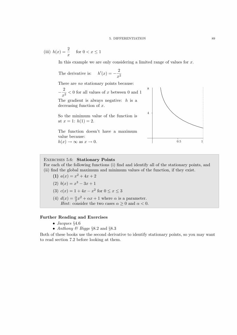
5. DIFFERENTIATION 89
(iii) h(x) =2x
for 0 < x 1
In this example we are only considering a limited range of values for x.
The derivative is: h
0(x) = �2x
2
There are no stationary points because:
�
2x
2< 0 for all values of x between 0 and 1
The gradient is always negative: h is adecreasing function of x.
So the minimum value of the function isat x = 1: h(1) = 2.
The function doesn’t have a maximumvalue because:h(x)!1 as x! 0.
.
..................................
.................................
................................
................................
...............................
........................
......
..........................
....
..............................
.
..................................
....................................
......................................
........................................
...........................................
.............................................
0.5 1
4
8
Exercises 5.6: Stationary Points
For each of the following functions (i) find and identify all of the stationary points, and(ii) find the global maximum and minimum values of the function, if they exist.
(1)(1) a(x) = x
2 + 4x + 2
(2) b(x) = x
3� 3x + 1
(3) c(x) = 1 + 4x� x
2 for 0 x 3
(4) d(x) = ↵
2 x
2 + ↵x + 1 where ↵ is a parameter.Hint : consider the two cases ↵ � 0 and ↵ < 0.
Further Reading and Exercises
• Jacques §4.6• Anthony & Biggs §8.2 and §8.3
Both of these books use the second derivative to identify stationary points, so you may wantto read section 7.2 before looking at them.

90 5. DIFFERENTIATION
⌥⌃
⌅⇧7. The Second Derivative
• The derivative y
0(x) tells us the gradient, or in other words how y changes as x increases.• But y
0(x) is a function.• So we can di↵erentiate y
0(x), to find out how y
0(x) changes as x increases.
The derivative of the derivative is called the second derivative. It can be denoted y
00(x), butthere are alternatives:
For the function y(x) the derivatives can be written:
1st derivative: y
0(x) ord
dx
(y(x)) ordy
dx
2nd derivative: y
00(x) ord
dx
✓dy
dx
◆or
d
2y
dx
2
Examples 7.1: Second Derivatives
(i) f(x) = ax
2 + bx + c
The 1st derivative is: f
0(x) = 2ax + b
Di↵erentiating again: f
00(x) = 2a
(ii) y =5x
2
This function can be written as y = 5x
�2 so:
First derivative:dy
dx
= �10x
�3 = �
10x
3
Second derivative:d
2y
dx
2= 30x
�4 =30x
4
Exercises 5.7: Find the first and second derivatives of:(1)(1) f(x) = x
4 (2) g(x) = x + 1 (3) h(x) = 4x
12 (4) k(x) = x
3(5x
2 + 6)
7.1. Using the Second Derivative to Find the Shape of a Function
• The 1st derivative tells you whether the gradient is positive or negative.• The 2nd derivative tells you whether the gradient is increasing or decreasing.
. ..................... ............................................
......................
.......................
........................
...........................
..............................
.................................
...................................
.
...................................
.................................
..............................
...........................
........................
.......................
............................................
...................... ..................... .
..................................
................................
.............................
...........................
........................
.......................
.......................
........................ ........................ ........................
. ........................ ........................ ..........................................
.....
.......................
........................
...........................
.............................
................................
..................................
f
0(x) > 0 Positive Gradient f
0(x) < 0 Negative Gradient
f
00(x) > 0 f
00(x) < 0 f
00(x) > 0 f
00(x) < 0Gradient increasing Gradient decreasing Gradient increasing Gradient decreasing

5. DIFFERENTIATION 91
Examples 7.2: y = x
3
From the derivatives of this function:dy
dx
= 3x
2 andd
2y
dx
2= 6x
we can see:
• There is one stationary point, at x = 0and at this point y = 0
• When x < 0:dy
dx
> 0 andd
2y
dx
2< 0
The gradient is positive, and decreasing.• When x > 0:
dy
dx
> 0 andd
2y
dx
2> 0
The gradient is positive, and increasing. .
.................................
...............................
..............................
............................
..........................
..........................
............................
.............................................................
................................. . ................................................................
..............................
............................
..........................
..........................
............................
..............................
...............................
.................................
7.2. Using the 2nd
Derivative to Classify Stationary Points
In section 6.3 we looked at the gradient on either side of a stationary point to determine itstype. But instead we can look at the sign of the second derivative, to see whether the gradientis increasing (as it will be at a minimum point, from negative to positive) or decreasing (asit will be at a maximum point, from positive to negative).
If f(x) has a stationary point at x = x0
(that is, if f
0(x0) = 0)
then if f
00(x0) > 0 it is a minimum pointand if f
00(x0) < 0 it is a maximum point
If the second derivative is zero it doesn’t help you to classify the point,and you have to revert to the previous method.
Examples 7.3: Applying this method to the examples in section 6.3:
(i) f(x) = x
2� 2x
f
0(x) = 2x� 2There is one stationary point at x = 1.
f
00(x) = 2
This is positive, for all values of x. So the stationary point is a minimum.
(ii) g(x) = 2x
3�
34x
4
g
0(x) = 6x
2� 3x
3 = 3x
2(x� 2)There are two stationary points, at x = 0 and x = 2.
g
00(x) = 12x� 9x
2 = 3x(4� 3x)
Look at each stationary point:

92 5. DIFFERENTIATION
x = 0: g
00(0) = 0 – we can’t tell its type. (We found beforethat it is a point of inflection.)
x = 2: g
00(2) = �12 – it is a maximum point.
Exercises 5.8: Find and classify all the stationary points of the following functions:(1)(1) a(x) = x
3� 3x
(2) b(x) = x +9x
+ 7
(3) c(x) = x
4� 4x
3� 8x
2 + 12
7.3. Concave and Convex Functions
If the gradient of a function is increasing for all values of x, the function is called convex.If the gradient of a function is decreasing for all values of x, the function is called concave.Since the second derivative tells us whether the gradient is increasing or decreasing:
A function f is called⇢
concaveconvex
�if
f
00(x)⇢
�
�0 for all values of x
.
..........
..........
..........
.......
..................................
................................
.............................
..........................
.......................
....................
.................
..............
............ ............ ........... ............ ............................................
..................
......................
.........................
............................
...............................
..................................
......................................
.........................................
.......................
...................
...................................
................ ............... ............... ................ ...............................
....
....................
........................
...........................
..............................
..................................
.....................................
........................................
...........................................
. ..........................................................
..........................................................
............................
............................
.............................
................................
..................................
.....................................
Convex
Concave
Convex
Examples 7.4: Are the following functions concave, convex, or neither?
(i) The quadratic function f(x) = ax
2 + bx + c.
f
00(x) = 2a, so if a > 0 it is convex and if a < 0 it is concave.
(ii) P (q) =1q
2
P
0(q) = �2q
�3, and P
00(q) = 6q
�4 =6q
4
The second derivative is positive for all values of q, so the function is convex.
(iii) y = x
3
We looked at this function in section 7.1. The second derivative changes sign, so thefunction is neither concave nor convex.

5. DIFFERENTIATION 93
7.4. Economic Application: Production Functions
The economic characteristics of a production function Y (L) depend on its shape:� It is (usually) an increasing function: Y
0(L) > 0 for all values of x;� but the second derivative could be positive or negative: it tells you whether the
marginal product of labour is increasing or decreasing.
.
.......................................
.....................................
...................................
..................................
................................
.................................
..................................
...................................
...........................................................................
...............................................................................
L
Y (i)
� Y
00(L) < 0 for all values of L
� The production function is concave� MPL is decreasing� Diminishing returns to labour
. ..................... .........................................
.......................................
...................
......................
........................
.
.....................................
..................................
...............................
............................
...........................
.....................................................
.................................................
L
Y (ii) This function is neither concave nor convex.When employment is low:
� Y
00(L) > 0� Increasing returns to labour
But when emplyment is higher:� Y
00(L) < 0� Decreasing returns to labour
Exercises 5.9: Concave and Convex Functions in Economics
(1)(1) Consider the cost function C(q) = 3q
2 + 2q + 5
(a) What is the marginal cost?
(b) Use the second derivative to find out whether the firm has increasing ordecreasing marginal cost.
(c) Is the cost function convex or concave?
(2) For the aggregate consumption function is C(Y ) = 10 + Y
0.9
(a) Find the first and second derivatives.
(b) How does the marginal propensity to consume change as income increases?
(c) Is the function concave or convex?
(d) Sketch the function.
Further Reading and Exercises
• Jacques §4.3 on the derivatives of economic functionsand §4.6 on maxima and minima
• Anthony & Biggs §8.2 and §8.3 for stationary points, maxima and minima

94 5. DIFFERENTIATION
Solutions to Exercises in Chapter 5
Exercises 5.1:(1) dy
dx
���x=2
= 9
Exercises 5.2:(1) dy
dx
= 4x
3,dy
dx
���x=�2
= �32
(2) dy
dx
= 32x
12 ,
dy
dx
���x=16
= 6
(3) dy
dx
���x=1
= 7(4) z
0(t) = 2t, z
0(3) = 6(5) Q
0(P ) = 1.7P
0.7
(6) u
0(y) = 56y
� 16 , u
0(1) = 56
(7) dy
dx
= �3x
4 , dy
dx
���x=2
= � 316
(8) dQ
dP
= � 1P
2
(a) limP!0
dQ
dP
= �1(b) lim
P!1dQ
dP
= 0
Exercises 5.3:(1) lim
h!0(x+h)3�x
3
h
=lim
h!03x
2h+3xh
2+h
3
h
=lim
h!0 3x
2 + 3xh + h
2 =3x
2
(2) limh!0
1x+h
� 1x
h
=lim
h!0x�x�h
x(x+h) .1h
=lim
h!0�1
x
2+xh
= �1x
2
(3) dy
dx
= 6x + 5
Exercises 5.4:(1) (a) f
0(x) = 16x
(b) f
0(2) = 32(c) f
0(0) = 0
(2) (a) u
0(y) = 40y
3� 2y
(b) v
0(y) = 7� 12y
(3) Q
0(P ) = 20P
3 �20P
2
= 20P
3 (1� P )(4) h
0(2) = 80(5) dy
dt
= 1� 12p
t
(6) g
0(x) = 6x + 2x
� 54 ,
g
0(1) = 8(7) y
0(x) =48x
3 + 21x
2� 8x� 2
(8) F
0(1) = 6
Exercises 5.5:(1) MPL = 200L
� 13 ,
MPL(8) = 100(2) C
0(Q) = 2kQ
k�1
(a) k > 1(b) k = 1(c) k < 1
(3) (a) C(50) ⇡ 43.81(b) C
0(Q) ⇡ 0.61
Exercises 5.6:(1) x = �2, a(�2) = �2:
global minimum.(2) x = �1, b(�1) = 3:
maximum point.x = 1, b(1) = �1:minimum point.No global max or min.
(3) x = 2, c(2) = 5:global maximum.No other stationarypoints; global minimum(in range 0 x 3) is atx = 0, c(0) = 1.
(4) Stationary point atx = 1, d(1) = 3
2↵ + 1.
It is a global max if ↵ < 0and a global min if ↵ > 0
Exercises 5.7:(1) f
0(x) = 4x
3
f
00(x) = 12x
2
(2) g
0(x) = 1g
00(x) = 0(3) h
0(x) = 2x
� 12
h
00(x) = �x
� 32
(4) k
0(x) = 25x
4 + 18x
2
k
00(x) = 100x
3 + 36x
Exercises 5.8:(1) (�1, 2) max
(1,�2) min(2) (�3, 1) max
(3, 13) min(3) (�1, 9) min
(0, 12) max(4,�116) min
Exercises 5.9:(1) (a) C
0(q) = 6q + 2(b) C
00(q) = 6)increasing MC
(c) convex(2) (a) C
0(Y ) = 0.9Y
�0.1,C
00(Y ) =� 0.09Y
�1.1
(b) It decreases(c) Concave
1This Version of Workbook Chapter 5: September 24, 2010

5. DIFFERENTIATION 95
⌥⌃ ⌅⇧Worksheet 5: Di↵erentiation
Quick Questions
(1) Di↵erentiate:(a) y = 9x
3� 7x
2 + 15
(b) f(x) =3
4x
2
(c) Y (t) = 100t
1.3
(d) P (Q) = Q
2� 4Q
12
(2) Determine whether each of the following functions is concave, convex, or neither:(a) y = 5x
2� 8x + 7
(b) C(y) =p
4y (for y � 0)(c) P (q) = q
2� 4q
12 (for q � 0)
(d) k(x) = x
2� x
3
(3) Find the first and second derivatives of the production function F (L) = 100L+200L
23
(for L � 0) and hence determine whether the firm has decreasing, constant, or in-creasing returns to labour.
(4) Find and classify all the the stationary points of the following functions. Find theglobal maxima and minima, if they exist, and sketch the functions.(a) y = 3x� x
2 + 4 for values of x between 0 and 4.(b) g(x) = 6x
12� x for x � 0.
(c) f(x) = x
4� 8x
3 + 18x
2� 5 (for all values of x)
(5) If a firm has cost function C(Q) = aQ(b + Q
1.5) + c, where a, b and c are positiveparameters, find and sketch the marginal cost function. Does the firm have concaveor convex costs?
Longer Questions
(1) The number of meals, y, produced in a hotel kitchen depends on the number of
cooks, n, according to the production function y(n) = 60n�
n
3
5
(a) What is the marginal product of labour?(b) Does the kitchen have increasing, constant, or decreasing returns to labour?(c) Find:
(i) the output of the kitchen(ii) the average output per cook(iii) the marginal product of labour
when the number of cooks is 1, 5, 10 and 15.(d) Is this a realistic model of a kitchen? Suggest a possible explanation for the
figures you have obtained.(e) Draw a careful sketch of the production function of the kitchen.(f) What is the maximum number of meals that can be produced?
(2) A manufacturer can produce economics textbooks at a cost of £5 each. The text-book currently sells for £10, and at this price 100 books are sold each day. The

96 5. DIFFERENTIATION
manufacturer figures out that each pound decrease in price will sell ten additionalcopies each day.(a) What is the demand function q(p) for the textbooks?(b) What is the cost function?(c) What is the inverse demand function?(d) Write down the manufacturer’s daily profits as function of the quantity of text-
books sold, ⇧(q).(e) If the manufacturer now maximises profits, find the new price, and the profits
per day.(f) Sketch the profit function.(g) If the government introduces a law that at least 80 economics textbooks must
be sold per day, and the (law-abiding) manufacturer maximises profits, find thenew price.

CHAPTER 6
More Di↵erentation, and Optimisation
In the previous chapter we di↵erentiated simple functions: powers ofx, and polynomials. Now we introduce further techniques of di↵erenti-ation, such as the product, quotient and chain rules, and the rulesfor di↵erentiating exponential and logarithmic functions. We usedi↵erentiation in a variety of economic applications: for example, to findthe profit-maximising output for a firm, the growth rate of GDP,the elasticity of demand and the optimum time to sell an asset.
—./—↵⌦
� 1. Graph Sketching
The first step towards understanding an economic model is often to draw pictures: graphsof supply and demand functions, utility functions, production functions, cost functions, andso on. In previous chapters we have used a variety of methods, including di↵erentiation, towork out the shape of a function. Here it is useful to summarise them, so that you can usethem in the economic applications in this chapter.
1.1. Guidelines for Sketching the Graph of a Function y(x)
• Look at the function y(x) itself:– to find where it crosses the x- and y-axes (if at all), and whether it is positive
or negative elsewhere;– to see what happens to y when x goes towards ±1;– to see whether there are any values of x for which y goes to ±1.
• Look at the first derivative y
0(x) to find the gradient:– It may be positive for all values of x, so the function is increasing;
or negative for all values of x, so the function is decreasing.– Otherwise, find the stationary points where y
0(x) = 0, and check whether thegraph slopes up or down elsewhere.
• Look at the second derivative y
00(x) to see which way the function curves:– Use it to check the types of the stationary points.– It may be positive for all values of x, so the function is convex;
or negative for all values of x, so the function is concave.– Otherwise, it tells you whether the gradient is increasing or decreasing in dif-
ferent parts of the graph.
Depending on the function, you may not need to do all of these things. Sometimes someof them are too di�cult – for example, you may try to find where the function crosses the
97

98 6. MORE DIFFERENTATION, AND OPTIMISATION
x-axis, but end up with an equation that you can’t solve. But if you miss out some steps, theothers may still give you enough information to sketch the function. The following exampleillustrates the procedure.
Examples 1.1: Sketch the graph of the function y(x) = 2x
3� 3x
2� 12x
(i) y(0) = 0, so it crosses the y-axis at y = 0
(ii) To find where it crosses the x-axis, we need to solve the equation y(x) = 0:
2x
3� 3x
2� 12x = 0
x(2x
2� 3x� 12) = 0
One solution of this equation is x = 0. To find the other solutions we need to solvethe equation 2x
2� 3x� 12 = 0. There are no obvious factors, so we use the quadratic
formula:
2x
2� 3x� 12 = 0
x =3±p
1054
x ⇡ 3.31 or x ⇡ �1.81
So the function crosses the x-axis at �1.81, 0, and 3.31.
(iii) What happens to y(x) = 2x
3� 3x
2� 12x as x becomes infinite?
For a polynomial, it is the term with the highest power of x that determines whathappens when x becomes infinite – it dominates all the other terms. In this case:
2x
3!1 as x!1, so y(x)!1 as x!1
2x
3! �1 as x! �1, so y(x)! �1 as x! �1
(iv) Are there any finite values of x that make y(x) infinite?No; we can evaluate y(x) for all finite values of x.
(v) The first derivative of the function is:
y
0(x) = 6x
2� 6x� 12
Stationary points occur where y
0(x) = 0:
6x
2� 6x� 12 = 0x
2� x� 2 = 0
(x + 1)(x� 2) = 0x = �1 or x = 2
So there are stationary points at x = �1, y = 7 and x = 2, y = �20
(vi) The second derivative of the function is:
y
00(x) = 12x� 6
At (�1, 7), y
00(x) = �18 so this is a maximum point.At (2,�20), y
00(x) = 18 so this is a minimum point.
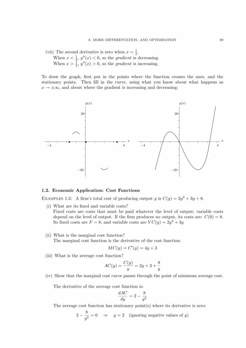
6. MORE DIFFERENTATION, AND OPTIMISATION 99
(vii) The second derivative is zero when x = 12 .
When x <
12 , y
00(x) < 0, so the gradient is decreasing.When x >
12 , y
00(x) > 0, so the gradient is increasing.
To draw the graph, first put in the points where the function crosses the axes, and thestationary points. Then fill in the curve, using what you know about what happens asx! ±1, and about where the gradient is increasing and decreasing:
y(x)
x
�4 4
�20
20
• • •
. ........... .......... ......... ......... .....................
. ........................ ......... ......... ........... .............
y(x)
x
�4 4
�20
20
.....................
......................
........................
...........................
.............................
...............................
..................................
....................................
......................
..................
................................................. ......... .......... ........... ............
...........................
....
....................
........................
......................................................
.
..................................
...............................
............................
........................
.....................
..................
...............
............. ............ ........... .......... .....................................
.................
....................
.......................
..........................
.............................
................................
.
...........................................................................................................................................................................................................................................................................................................................
1.2. Economic Application: Cost Functions
Examples 1.2: A firm’s total cost of producing output y is C(y) = 2y
2 + 3y + 8.
(i) What are its fixed and variable costs?Fixed costs are costs that must be paid whatever the level of output; variable costsdepend on the level of output. If the firm produces no output, its costs are: C(0) = 8.So fixed costs are F = 8, and variable costs are V C(y) = 2y
2 + 3y
(ii) What is the marginal cost function?The marginal cost function is the derivative of the cost function:
MC(y) = C
0(y) = 4y + 3
(iii) What is the average cost function?
AC(y) =C(y)
y
= 2y + 3 +8y
(iv) Show that the marginal cost curve passes through the point of minimum average cost.
The derivative of the average cost function is:dAC
dy
= 2�8y
2
The average cost function has stationary point(s) where its derivative is zero:
2�8y
2= 0 ) y = 2 (ignoring negative values of y)

100 6. MORE DIFFERENTATION, AND OPTIMISATION
Look at the second derivative to see if this is a miminum:d
2AC
dy
2=
16y
3
Since this is positive when y = 2 we have found a minimum point. At this point:
y = 2, AC(y) = 11 and MC(y) = 11
So the marginal cost curve passes through the point of minimum average cost.
(v) Sketch the marginal and average cost functions.We will sketch the functions for positive values of y only, since negative values are of noeconomic interest. Sketching MC(y) is easy: it is a straight line, of gradient 4, crossingthe vertical axis at 3, and (from above) passing throught the point (2,11).For the average cost function:
AC(y) =C(y)
y
= 2y + 3 +8y
we already know that it has one stationary point, which is a minimum. Also, we havefound the second derivative, and it is positive for all positive values of y, so the gradientis always increasing.We can see by looking at AC(y) that as y ! 0, AC(y) ! 1, and that as y ! 1,AC(y)!1. The function does not cross either of the axes.
.
..................................................................................................................................................................................................................................................................................................................................................................................................................................................................................................................................................................................................................................................................................................................
.
..........
..........
..........
..........
...
..........
..........
..........
..........
.
..........
..........
..........
........
....................................
.................................
..............................
............................
.........................
......................
....................
..................
.................. .................. .................. .................. . .......................................................................................................
........................................................
...........................................................
..............................................................
.................................................................
....................................................................
.......................................................................
.........................................................................
Cost
y
10
20
642
MC(y)
AC(y)
Exercises 6.1: Sketching Graphs(1)(1) Sketch the graphs of the functions:
(a) a(x) = (1� x)(x� 2)(x� 3) (b) b(x) = x
12 (x� 6) for x � 0.
(2) A firm has cost function C(y) = y
3 + 54. Show that the marginal cost functionpasses through the point of minimum average cost, and sketch the marginal andaverage cost functions.
(3) A firm has cost function C(y) = 2y + 7. Sketch the marginal and average costfunctions.

6. MORE DIFFERENTATION, AND OPTIMISATION 101
↵⌦
� 2. Introduction to Optimisation
In economic applications we often want to find the (global) maximum or minimum of afunction. For example, we may want to find:
• the level of output where a firm’s profit is maximised• the level of output where a firm’s average cost of production is minimised• the number of hours per week that an individual should work, if he wants to maximise
his utility.Usually in economic applications the relevant function just has one stationary point, and thisis the maximum or minimum that we want. But, having found a stationary point it is alwayswise to check that it is a maximum or minimum point (whichever is expected) and that it isa global optimum.
2.1. Profit Maximisation
Suppose that a firm producing y units of output has cost function C(y), and faces inversedemand function P (y). (In other words, if the firm makes y units, the total cost is C(y), andeach unit can be sold at a price P (y).)
• The firm’s Revenue Function is: R(y) = yP (y)
• The firm’s Profit Function is: ⇧(y) = R(y)� C(y) = yP (y)� C(y)
• The firm’s optimal choice of output is the value of y that maximises its profit ⇧(y).
So we can find the optimal output by finding the maximum point of the profit function.
Examples 2.1: A monopolist has inverse demand function P (y) = 16�2y and cost functionC(y) = 4y + 1.
(i) What is the optimal level of output?The profit function is:
⇧(y) = y(16� 2y)� (4y + 1)= 12y � 2y
2� 1
Look for a maximum point where the derivative is zero:d⇧dy
= 12� 4y = 0 ) y = 3
To check that this is a maximum look at the second derivative:d
2⇧dy
2= �4 so it is a maximum
If you think about the shape of the function (or sketch it), you can see that this theglobal maximum. So the optimal choice of output is y = 3.
(ii) How much profit does it make?When y = 3:
⇧(3) = 12⇥ 3� 2⇥ 9� 1 = 17Profit is 17.
102 6. MORE DIFFERENTATION, AND OPTIMISATION
2.2. Marginal Cost, Marginal Revenue, and Profit Maximisation
We know that Marginal Cost is the cost of an additional unit of output, which is the derivativeof the cost function:
MC(y) =dC
dy
Similarly Marginal Revenue is the revenue obtained when one more unit of output is sold,and it is the derivative of the revenue function:
MR(y) =dR
dy
To find the optimal level of output, we look for the point whered⇧dy
= 0.
But we can write the profit function as:
⇧(y) = R(y)� C(y)
)
d⇧dy
=dR
dy
�
dC
dy
So the optimal level of output is where:dR
dy
=dC
dy
) Marginal Revenue = Marginal Cost
The optimal level of output for a profit-maximising firm is
whered⇧dy
= 0, or (equivalently) where MR = MC
If you want to find the profit-maximising output you can either look for a stationary pointof the profit function, or solve the equation MR = MC.
Exercises 6.2: Introduction to Optimisation(1)(1) A competitive firm has cost function C(q) = 3q
2 + 1. The market price is p =24. Write down the firm’s profit as a function of output, ⇧(q). Find the profit-maximising level of output. How much profit does the firm make if it producesthe optimal amount of output?
(2) A monopolist faces demand curve Q
d(P ) = 10 � 0.5P . Find the inverse demandfunction P
d(Q), and hence the revenue function R(Q), and marginal revenue.Suppose the monopoly wants to maximise its revenue. What level of output shouldit choose?
(3) A competitive firm produces output using labour as its only input. It has no fixedcosts. The production function is y = 6L
0.5; the market price is p = 4, and thewage (the cost of labour per unit) is w = 2. Write down the firm’s profit, as afunction of the number of units of labour it employs, ⇧(L). How many units oflabour should the firm employ if it wants to maximise its profit?
Further Reading and Exercises• Jacques §4.6.• Anthony & Biggs §8.1, 8.2.

6. MORE DIFFERENTATION, AND OPTIMISATION 103
⌥⌃
⌅⇧3. More Rules for Di↵erentiation
3.1. Product Rule
To di↵erentiate the function:
y(x) = (5x + 3)(x2� x + 1)
we could multiply out the brackets and di↵erentiate as before. Alternatively we could use:
The Product Rule: If y(x) = u(x)v(x) then
y
0(x) = u(x)v0(x) + u
0(x)v(x)
or equivalently
dy
dx
= u
dv
dx
+ v
du
dx
Examples 3.1: Product Rule
(i) Di↵erentiate y(x) = (5x + 3)(x2� x + 1)
Put u(x) = 5x + 3, and v(x) = x
2� x + 1:
dy
dx
= (5x + 3)(2x� 1) + 5(x2� x + 1)
= 15x
2� 4x + 2
(ii) Di↵erentiate 2x
32 (x3
� 2)f(x) = 2x
32 (x3
� 2)
Put u(x) = 2x
32 and v(x) = x
3� 2:
f
0(x) = 2x
32⇥ 3x
2 + 3x
12 (x3
� 2)
= 9x
72� 6x
12
3.2. Quotient Rule
So far we have no method for di↵erentiating a function such as:
y(x) =3x� 22x + 1
but there is a rule for di↵erentiating the quotient of two functions:
The Quotient Rule: If y(x) =u(x)v(x)
then
y
0(x) =u
0(x)v(x)� u(x)v0(x)v(x)2
or equivalently:dy
dx
=v
du
dx
� u
dv
dx
v
2

104 6. MORE DIFFERENTATION, AND OPTIMISATION
Examples 3.2: Quotient Rule
(i) Di↵erentiate g(x) =3x� 22x + 1
Putting u = 3x� 2 and v = 2x + 1:dg
dx
=(2x + 1)⇥ 3� (3x� 2)⇥ 2
(2x + 1)2
=6x + 3� 6x + 4
(2x + 1)2=
7(2x + 1)2
(ii) Di↵erentiate h(x) =3x
x
2 + 2
h
0(x) =(x2 + 2)⇥ 3� 3x⇥ 2x
(x2 + 2)2=
3x
2 + 6� 6x
2
(x2 + 2)2=
6� 3x
2
(x2 + 2)2
3.3. Chain Rule
To di↵erentiate the function:y(x) = 4(2x
3� 1)7
we could multiply out the brackets to obtain a very long polynomial (of degree 21) and thendi↵erentiate. But this would take a very long time. Instead we can do it by writing y as afunction of a function:
y = 4u
7 where u = 2x
3� 1
and then using the Chain Rule:
The Chain RuleIf y is a function of u, and u is a function of x:
dy
dx
=dy
du
⇥
du
dx
Applying this to the example above:dy
dx
= 28u
6⇥ 6x
2
= 28(2x
3� 1)6 ⇥ 6x
2
= 168x
2(2x
3� 1)6
The Chain Rule is the rule for di↵erentiating a composite function (see Chapter 4). Anotherway of writing it is:
Alternative Form of the Chain RuleIf y(x) = v(u(x))
y
0(x) = v
0(u(x))u0(x)

6. MORE DIFFERENTATION, AND OPTIMISATION 105
Examples 3.3: Di↵erentiate the following functions using the Chain Rule:
(i) y(x) = (1� 8x)5
y = u
5 where u = 1� 8x
dy
dx
= 5u
4⇥ (�8) = 5(1� 8x)4 ⇥ (�8) = �40(1� 8x)4
(ii) f(x) =p
(2x� 3)First write this as: f(x) = (2x� 3)
12 . Then:
f = u
12 where u = 2x� 3
f
0(x) =12u
� 12⇥ 2
=12(2x� 3)�
12⇥ 2
=1
p
2x� 3
(iii) g(x) =1
1 + x
2
g =1u
where u = 1 + x
2
g
0(x) = �
1u
2⇥ 2x
= �
2x
(1 + x
2)2
(Note that we could have done this example using the quotient rule.)
3.4. Di↵erentiating the Inverse Function
x
y
. ............................................................
.............................
.............................
.............................
.............................
...............................
..................................
....................................
......................................
.........................................
�x
�y
Remember from Chapter 5 that the derivative of a function isapproximately equal to the ratio of the change in y to the changein x as you move along the function:
dy
dx
⇡
�y
�x
If a function has an inverse:
y = f(x) and x = f
�1(y)
then the gradients of these two functions are:dy
dx
⇡
�y
�x
anddx
dy
⇡
�x
�y
So the gradient of the inverse function f
�1 =1
the gradient of the function f
dx
dy
=1dy
dx
We will use this rule in later sections of this chapter.

106 6. MORE DIFFERENTATION, AND OPTIMISATION
Exercises 6.3: More Rules for Di↵erentiation(1)(1) Use the product rule to di↵erentiate:
(a) y(x) = (x2 + 3x + 2)(x� 1) (b) f(z) = z(1�p
z)
(2) Use the quotient rule to di↵erentiate: k(x) =x + 1
2x
3 + 1
(3) Use the chain rule to di↵erentiate: (a) a(x) = 2(2x� 7)9 (b) b(y) =p
y
2 + 5
(4) For a firm facing inverse demand function P (y) =1
2y + 3, find the revenue function
R(y), and the marginal revenue.
3.5. More Complicated Examples
Examples 3.4: Sometimes we need more than one of the product, quotient and chain rules:
(i) Di↵erentiate the function y(x) = x
3(x2 + 1)4.
By the Product Rule:dy
dx
= x
3⇥
d
dx
�(x2 + 1)4
+ 3x
2⇥ (x2 + 1)4
Then use the Chain Rule to di↵erentiate the term in curly brackets:dy
dx
= x
3⇥ 4(x2 + 1)3 ⇥ 2x + 3x
2(x2 + 1)4
= 8x
4(x2 + 1)3 + 3x
2(x2 + 1)4
Factorising:dy
dx
= x
2(x2 + 1)3(11x
2 + 3)
(ii) Di↵erentiate: f(x) =✓
x
x + ↵
◆�
First use the Chain Rule, with u = x
x+↵
:
f
0(x) = �
✓x
x + ↵
◆��1
d
dx
⇢x
x + ↵
�
Then use the Quotient Rule to di↵erentiate the term in curly brackets:
f
0(x) = �
✓x
x + ↵
◆��1 ✓
↵
(x + ↵)2
◆= ↵�
x
��1
(x + ↵)�+1
Exercises 6.4:
(1)(1) Find the derivative of y(x) =r
x
1� x
(2) Di↵erentiate z(t) =t
a
(2t + 1)b
where a and b are parameters.
(3) If f(q) = q
5(1� q)3, for what values of q is f(q) increasing?
(4) (Harder) Using the chain rule and the product rule, derive the quotient rule.
Further Reading and Exercises• Jacques §4.4.• Anthony & Biggs §6.2, §6.4 and §6.5.

6. MORE DIFFERENTATION, AND OPTIMISATION 107
↵⌦
� 4. Economic Applications
4.1. Minimum Average Cost
If a firm has total cost function C(q), where q is its output, its average cost function is:
AC(q) =C(q)
q
The derivative of the average cost function can be found using the Quotient Rule:dAC
dq
=qC
0(q)� C(q)q
2
At a point where average cost is minimised,dAC
dq
= 0, so:
qC
0(q)� C(q) = 0
C
0(q) =C(q)
q
MC = AC
We have proved that for any cost function, MC = AC when AC is minimised: the marginalcost function passes through the minimum point of the average cost function.
4.2. The Marginal Revenue Product of Labour
If a firm uses labour to produces its output y, with production function f(L), revenue is afunction of output, and output is a function of labour:
Revenue = R(y) where y = f(L)
The marginal revenue product of labour is the additional revenue generated by employing onemore unit of labour:
MRPL =dR
dL
Using the chain rule:dR
dL
=dR
dy
⇥
dy
dL
= MR⇥MPL
The marginal revenue product of labour is the marginal revenue multiplied by the marginalproduct of labour.
Exercises 6.5:(1)(1) A firm has cost function C(q) = (q +2)� where � is a parameter greater than one.
Find the level of output at which average cost is minimised.
(2) A firm produces output Q using labour L. Its production function is Q = 3L
13 . If
it produces Q units of output, the market price will be P (Q) =54
Q + 9.
(a) What is the firm’s revenue function R(Q)?
(b) If the firm employs 27 units of labour, find: (i) output (ii) the marginal prod-uct of labour (iii) the market price (iv) marginal revenue (v) the marginalrevenue product of labour

108 6. MORE DIFFERENTATION, AND OPTIMISATION
↵⌦
� 5. Economic Application: Elasticity
5.1. The Price Elasticity of Demand
The gradient dq
dp
of a demand curve q(p) gives a measure of how “responsive” demand is toprice: how much demand falls (it is usually negative) when price rises a little:
dq
dp
⇡
�q
�p
But the gradient depends on the units in which price and quantity are measured. So, forexample, the demand for cars in the UK would appear by this measure to be more responsiveto price than in the US, simply because of the di↵erence in currencies.
A better measure, which avoids the problem of units, is the elasticity, which measures theproportional change in quantity in response to a small proportional change in price. Theprice elasticity of demand is the answer to the question “By want percentage would demandchange, if the price rose by one percent?”
Price elasticity of demand, ✏ =p
q
dq
dp
You can see where this definition comes from if we write:
p
q
dq
dp
⇡
p
q
�q
�p
=�q/q
�p/p
=proportional change in q
proportional change in p
Examples 5.1: For the demand function q(p) = 10� 2p:
(i) Find the price elasticity of demand.dq
dp
= �2
) ✏ =p
q
⇥ (�2)
Substituting for q we obtain the elasticity as a function of price only:
✏ =�2p
10� 2p
(ii) Evaluate the elasticity when the price is 1, and when the price is 4.Substituting into the expression for the elasticity in (i):
when p = 1, ✏ = �14
and when p = 4, ✏ = �4
In this example, demand is inelastic (unresponsive to price changes) when the price is low,but elastic when price is high.
We say that demand is:• inelastic if |✏| < 1• unit-elastic if |✏| = 1• elastic if |✏| > 1

6. MORE DIFFERENTATION, AND OPTIMISATION 109
Warning : The price elasticity of demand is negative, but economists are often careless aboutthe minus sign, saying, for example “The elasticity is greater than one” when we mean thatthe absolute value of the elasticity, |✏|, is greater than one. Also, some books define theelasticity as �p
q
dq
dp
, which is positive.
5.2. Manipulating Elasticities
In the example above we started from the demand function q(p) = 10� 2p, and obtained theelasticity as a function of price. But if we can find the inverse demand function, we couldexpress the elasticity as a function of quantity instead:
q = 10� 2p ) p = 5�q
2
Then:
) ✏ =p
q
⇥ (�2) (as before)
=q � 10
q
We can also find the price elasticity of demand if we happen to know the inverse demandfunction p(q), rather than the demand function. We can di↵erentiate to find its gradient dp
dq
.Then the gradient of the demand function is:
dq
dp
=1dp
dq
(from section 3.4) and we can use this to evaluate the elasticity.
Examples 5.2: If the inverse demand function is p = q
2� 20q + 100 (for 0 q 10), find
the elasticity of demand when q = 6.Di↵erentiatiating the inverse demand function and using the result above:
dp
dq
= 2q � 20 )
dq
dp
=1
2q � 20
) ✏ =p
q
12q � 20
Here, it is natural to express the elasticity as a function of quantity:
✏ =q
2� 20q + 100q(2q � 20)
Evaluating it when q = 6:
✏ =16
6⇥ (12� 20)= �
13
5.3. Elasticity and Revenue
If a firm faces inverse demand function p(q), its revenue function is:
R(q) = p(q)q
As quantity increases, more items are sold, but at a lower price. What happens to revenue?

110 6. MORE DIFFERENTATION, AND OPTIMISATION
Di↵erentiating, using the Product Rule, we obtain Marginal Revenue:dR
dq
= p + q
dp
dq
= p
✓1 +
q
p
dp
dq
◆
= p
1 +
1p
q
dq
dp
!
= p
✓1 +
1✏
◆
= p
✓1�
1|✏|
◆
From this expression we can see that revenue is increasing with quantity if and only if |✏| > 1:that is, if and only if demand is elastic.
5.4. Other Elasticities
We can define other elasticities in just the same way as the price elasticity of demand. Forexample:
• If q
s(p) is a supply function, the elasticity of supply isp
q
s
dq
s
dp
• If Y (L) is a production function,L
Y
dY
dL
is the elasticity of output with respect tolabour.
Exercises 6.6: Elasticity(1)(1) Find the price elasticity of demand for the demand function Q
d(P ) = 100 � 5P ,as a function of the price. What is the elasticity when P = 4?
(2) If the inverse demand function is p
d(q) = 10+ 20q
, find the price elasticity of demandwhen q = 4.
(3) Find the elasticity of supply, as a function of price, when the supply function is:q
s(p) =p
3p + 4.
(4) Show that demand function q
d(p) = ↵p
��, where ↵ and � are positive parameters,has constant elasticity of demand.
Further Reading and Exercises• Jacques §4.5.• Anthony & Biggs §9.1.• Varian “Intermediate Microeconomics” Chapter 15 discusses elasticity fully, without
using calculus in the main text, and using calculus in the Appendix.

6. MORE DIFFERENTATION, AND OPTIMISATION 111
✏�
��
6. Di↵erentiation of Exponential andLogarithmic Functions
6.1. The Derivative of the Exponential Function
The reason why the exponential function e
x is so important in mathematics and economicsis that it has a surprising property:1 the derivative of e
x is e
x.
If y = ex thendy
dx
= e
x
Using the chain rule we can show easily that if a is a constant:
If y = e
ax thendy
dx
= ae
ax
Examples 6.1: Di↵erentiate:
(i) 2e
3x
y = 2e
3x
)
dy
dx
= 2⇥ 3e
3x = 6e
3x
(ii) Y (t) = ae
�bt
Y
0(t) = a⇥ (�b)⇥ e
�bt = �abe
�bt
(iii) k(x) = 5e
x
4+2x
Using the chain rule: ) k
0(x) = 5e
x
4+2x
⇥ (4x
3 + 2)
= 5(4x
3 + 2)ex
4+2x
6.2. The Derivative of the Logarithmic Function
The logarithmic function lnx is the inverse of the exponential function, and we can use thisto find its derivative:
y = ln x ) x = e
y
dx
dy
= e
y = x
dy
dx
=1dx
dy
=1x
So we have obtained a rule for di↵erentiating lnx:
If y = ln x thendy
dx
=1x
1You could try to verify this by di↵erentiating ex
= lim
n!1�1 +
x
n
�n
.

112 6. MORE DIFFERENTATION, AND OPTIMISATION
Examples 6.2: Di↵erentiate the following functions:
(i) f(x) = ln(5x)
Again we can use the chain rule: f
0(x) =15x
⇥ 5 =1x
(ii) p(q) = 3 ln(q2� 5q)
p
0(q) = 3⇥1
q
2� 5q
⇥ (2q � 5) =3(2q � 5)q
2� 5q
Exercises 6.7: Di↵erentiation of Exponential and Logarithmic Functions(1)(1) Di↵erentiate the function: f(x) = 1
2e8x.
(2) What is the derivative of 4 ln(3x + 1)?
(3) Find the derivative of C(q) = 3qeq
2 + 4e
�2q.
(4) Di↵erentiate the function: g(y) = y
2 ln(2y)+2. For what values of y is g increasing?
(5) Find and classify the stationary points of the function: F (t) = e
�t(t2 + 2t� 2).
(6) If f(x) is any function, find the derivative of (a) y(x) = e
f(x) (b) z(x) = ln f(x).
6.3. Economic Application: Growth
In Chapter 4, we modelled the GDP of a country as depending on time, according to theequation:
Y (t) = Y0e0.03t
(Remember that the parameter Y0 represents GDP at time t = 0.)Di↵erentiating this equation we get:
Y
0(t) = 0.03Y0e0.03t
= 0.03Y (t)
So we can now see that the rate of increase of GDP, Y
0(t), is a constant proportion, 0.03, ofGDP. In other words, GDP is growing at a rate of 3%.
6.4. Economic Application: The Optimum Time to Sell an Asset
F (t)
t.
........................................
.......................................
......................................
......................................
.....................................
........................................
..........................................
............................................
..............................................
................................................
...................................................
.....................................................Suppose that, as a forest grows over time,the value of the timber is given by F (t),where F is an increasing, concave, func-tion of time. Then, if the interest rate isr, the present value of the forest at time t
is:V (t) = F (t)e�rt
(See Chapter 3.)

6. MORE DIFFERENTATION, AND OPTIMISATION 113
The best time to cut down the forest and sell the timber is when the present value is max-imised. Di↵erentiating (using the product rule):
dV
dt
= F
0(t)e�rt
� rF (t)e�rt
= (F 0(t)� rF (t))e�rt
The optimum moment is whendV
dt
= 0:
F
0(t) = rF (t) )
F
0(t)F (t)
= r
This means that the optimum time to sell is when the proportional growth rate of the forestis equal to the interest rate. (You can verify, by di↵erentiating again, that this is a maximumpoint.)
To see why, call the optimum moment t
⇤. After t
⇤, the value of the forest is growing moreslowly than the interest rate, so it would be better to sell it and put the money in the bank.Before t
⇤, the forest grows fast: it o↵ers a better rate of return than the bank.
Exercises 6.8:(1)(1) A painting is bought as an investment for £3000. The artist is increasing in
popularity, so the market price is rising by £300 each year: P (t) = 3000 + 300t.If the interest rate is 4%, when should the painting be sold?
(2) The output Y of a country is growing at a proportional rate g and the populationN is growing at a proportional rate n:
Y (t) = Y0egt and N(t) = N0e
nt
Output per person is y(t) =Y (t)N(t)
. Using the quotient rule, show that the propor-
tional rate of growth of output per person is g � n.
Further Reading and Exercises• Jacques §4.8.• Anthony & Biggs §7.2 and §7.4.• For more discussion of “When to cut a forest” see Varian, “Intermediate Microeco-
nomics”, Chapter 11 and its Appendix.

114 6. MORE DIFFERENTATION, AND OPTIMISATION
Solutions to Exercises in Chapter 6
Exercises 6.1:(1) (a) Graph crosses y-axis
at y = 6 and x-axisat 1,2 and 3. Maxat x = 2.577; min atx = 1.423. a ! �1
as x ! 1 and a !
1 as x! �1.(b) Graph passes
through (0,0) andcrosses x-axis atx = 6. Min atx = 2, b = �5.66.Convex: b
00(x) > 0for all x. b ! 1 asx!1.
(2) MC = 3y
2; AC = y
2 +54y
. AC is minimisedwhen y = 3. At this pointMC = AC = 27.
(3) MC is a horizontalline MC = 2. AC isdownward-sloping andconvex. As y ! 0,AC !1, and as y !1,AC ! 2.
Exercises 6.2:(1) ⇧(q) = 24q � 3q
2� 1.
Profit is maximised whenq = 4. ⇧(4) = 47.
(2) P
d(Q) = 20� 2Q
R(Q) = (20� 2Q)QMR = 20� 4Q
Revenue is maximisedwhen Q = 5.
(3) ⇧(L) = 24L
0.5� 2L.
Profit is maximised whenL = 36.
Exercises 6.3:(1) (a) y
0(x) = 3x
2 + 4x� 1(b) f
0(z) = 1� 32
p
z
(2) k
0(x) = 1�4x
3�6x
2
(2x
3+1)2
(3) (a) a
0(x) = 36(2x� 7)8(b) b
0(y) = y
p
y
2+5
(4) R(y) = y
2y+3
MR = 3(2y+3)2
Exercises 6.4:(1) y
0(x) = 1
2x
12 (1�x)
32
(2) z
0(t) = t
a�1(a+2at�2bt)(2t+1)b+1
(3) f
0(q)= 5q
4(1�q)3�3q
5(1�q)2= q
4(1� q)2(5� 8q)So f is increasing whenq <
58 .
(4) Let y(x) = u(x)v(x) . Write it
as:y(x) = u(x) (v(x))�1
dy
dx
= du
dx
v
�1 + u
d
dx
{v
�1}
= du
dx
v
�1� uv
�2 dv
dx
= v
�2�v
du
dx
� u
dv
dx
�
= v
du
dx
�u
dv
dx
v
2
Exercises 6.5:(1) q = 2
��1
(2) (a) R(Q) = 54Q
Q+9
(b) (i) Q = 9(ii) MPL = 1
9(iii) P = 3(iv) MR = 3
2
(v) MRPL = 16
Exercises 6.6:
(1) ✏ = � 5P
100�5P
; ✏ = �14
(2) �3(3) 3p
2(3p+4)
(4) ✏ = �↵�p
���1⇥
p
q
= �↵�p
��
⇥
1q
= ��
Exercises 6.7:
(1) f
0(x) = 4e
8x
(2) 123x+1
(3) 3(1 + 2q
2)eq
2� 8e
�2q
(4) g
0(y) = y(1 + 2 ln(2y))Increasing when1 + 2 ln(2y) > 0) y >
1
2e
12
(5) Max at (2, 6e
�2)Min at (�2,�2e
2)(6) (a) y
0(x) = f
0(x)ef(x)
(b) z
0(x) = f
0(x)f(x)
Exercises 6.8:
(1) The present value is(3000 + 300t)e�0.04t.This is maximised whent = 15.
(2) y
0(t) = N(t)Y 0(t)�Y (t)N 0(t)N
2
But:Y
0 = gY and N
0 = nN
so:y
0 = gNY �nNY
N
2
= (g � n) Y
N
= (g � n)y
2This Version of Workbook Chapter 6: August 22, 2003

6. MORE DIFFERENTATION, AND OPTIMISATION 115
✏�
��
Worksheet 6: More Di↵erentiationand Optimisation
Quick Questions
(1) Find the derivatives of the following functions:
(a) f(x) = (2x + 1)(x + 3) (b) g(y) =y
2 + 12� y
(c) h(z) = (6z + 1)5
(2) For what values of the parameter a is y(x) =x + 1x + a
an increasing function of x?
(3) Di↵erentiate: (a) e
3x (b) ln(3x
2 + 1) (c) e
x
3 (d) e
2x(x + 1x
)
(4) If the cost function of a firm is C(q) = q
2p
1 + 2q, what is the marginal cost function?
(5) Does the production function F (L) = ln(2L + 5) have increasing or decreasing re-turns to labour?
(6) Consider the function:
y (x) =�2x
2� 2x� 1
�e
2x
(a) Find and classify the stationary points.(b) For what values of x is y positive?(c) Sketch the graph of the function.
(7) Find the elasticity of demand when the demand function is q(p) = 120 � 5p. Forwhat values of p is demand inelastic?
(8) Suppose that a monopoly has cost function C (q) = q
2, and a demand function
q (p) = 10 � p
2 . Find (i) the inverse demand curve; (ii) the profit function; and (iii)the profit-maximizing level of output, and corresponding price.
(9) The supply and demand functions in a market are
q
s (p) = 16(p� t) q
d (p) = 24� 8p
where t is a per unit sales tax. Find the equilibrium price and quantity in the mar-ket, and the total tax revenue for the government, in terms of the tax, t. What valueof t should the government choose if it wants to maximise tax revenue? How muchtax will then be raised?
Longer Questions
(1) Suppose that a monopolist faces the demand function: q
D (p) =a
p
2 + 1where a is a positive parameter.
(a) Find the elasticity of demand (i) as a function of the price, and (ii) as a functionof the quantity sold.
(b) At what value of q is the elasticity of demand equal to 1?(c) Sketch the demand curve, showing where demand is inelastic, and where it is
elastic.(d) Find the firm’s revenue function, and its marginal revenue function.
116 6. MORE DIFFERENTATION, AND OPTIMISATION
(e) Sketch the revenue function, showing where revenue is maximised.(f) Explain intuitively the relationship between the shape of the revenue function
and the elasticity of demand.(g) Prove that, in general for a downward-sloping demand function, marginal rev-
enue is zero when the elasticity is one. Is it necessarily true that revenue ismaximised at this point? Explain.
(2) For a firm with cost function C(y), the average cost function is defined by:
AC =C (y)
y
(a) If C(y) =2y
3
3+ y + 36:
(i) Find the fixed cost, the average cost function, and the marginal costfunction.
(ii) At what level of output is average cost minimised? What is the averagecost at this point?
(iii) Sketch carefully the average and marginal cost functions.
(b) If C(y) = cy + F where c and F are positive parameters:(i) Show that the average cost function is decreasing at all levels of output.(ii) Show that marginal cost is less than average cost for all values of y.(iii) Sketch the marginal and average cost functions.
(c) Prove that, for any cost function C(y), AC is decreasing whenever MC < AC,and AC is increasing whenever MC > AC (for y > 0). Explain intuitively whythis is so.
(3) The ageing bursar of St. Giles College and its young economist have disagreed aboutthe disposal of college wine. The Bursar would like to sell up at once, whereas sheis of the view that the college should wait 25 years. Both agree, however, that if thewine is sold t years from now, the revenue received will be:
W (t) = A exp(t12 )
and that the interest rate, r, will be stable.(a) Di↵erentiate W , and hence show that the proportional growth rate of the po-
tential revenue is1W
dW
dt
=1
2p
t
(b) Explain why the present value of the revenue received if the wine is sold in t
years is given by:
V (t) = A exp⇣t
12� rt
⌘
(c) Di↵erentiate V , and hence determine the optimum time to sell the wine.(d) Explain intuitively why the wine should be kept longer if the interest rate is
low.(e) If the interest rate is 10%, should the Governing Body support the Bursar or
the economist?

CHAPTER 7
Partial Di↵erentiation
From the previous two chapters we know how to di↵erentiate functionsof one variable. But many functions in economics depend on severalvariables: output depends on both capital and labour, for example. Inthis chapter we show how to di↵erentiate functions of several vari-ables and apply this to find the marginal products of labour andcapital, marginal utilities, and elasticities of demand. We usedi↵erentials to find the gradients of isoquants, and hence determinemarginal rates of substitution.
—./—⌥⌃
⌅⇧1. Partial Derivatives
The derivative of a function of one variable, such as y(x), tells us the gradient of the function:how y changes when x increases. If we have a function of more than one variable, such as:
z(x, y) = x
3 + 4xy + 5y2
we can ask, for example, how z changes when x increases but y doesn’t change. The answerto this question is found by thinking of z as a function of x, and di↵erentiating, treating y
as if it were a constant parameter:
@z
@x
= 3x2 + 4y
This process is called partial di↵erentiation. We write @z
@x
rather than dz
dx
, to emphasize thatz is a function of another variable as well as x, which is being held constant.
@z
@x
is called the partial derivative of z with respect to x
@z
@x
is pronounced “partial dee z by dee x”.
Similarly, if we hold x constant, we can find the partial derivative with respect to y:
@z
@y
= 4x+ 10y
Remember from Chapter 4 that you can think of z(x, y) as a “surface” in 3 dimensions.Imagine that x and y represent co-ordinates on a map, and z(x, y) represents the height ofthe land at the point (x, y). Then, @z
@x
tells you the gradient of the land as you walk in the
direction of increasing x, keeping the y co-ordinate constant. If @z
@x
> 0, you are walkinguphill; if it is negative you are going down. (Try drawing a picture to illustrate this.)
117
118 7. PARTIAL DIFFERENTIATION
Exercises 7.1: Find the partial derivatives with respect to x and y of the functions:
(1)(1) f(x, y) = 3x2 � xy
4 (3) g(x, y) =lnx
y
(2) h(x, y) = (x+ 1)2(y + 2)
Examples 1.1: For the function f(x, y) = x
3e
�y:
(i) Show that f is increasing in x for all values of x and y.
@f
@x
= 3x2e�y
Since 3x2 > 0 for all values of x, and e
�y
> 0 for all values of y, this derivative isalways positive: f is increasing in x.
(ii) For what values of x and y is the function increasing in y?
@f
@y
= �x
3e
�y
When x < 0 this derivative is positive, so f is increasing in y. When x > 0, f isdecreasing in y.
1.1. Second-order Partial Derivatives
For the function in the previous section:
z(x, y) = x
3 + 4xy + 5y2
we found:@z
@x
= 3x2 + 4y
@z
@y
= 4x+ 10y
These are the first-order partial derivatives. But we can di↵erentiate again to find second-order partial derivatives. The second derivative with respect to x tells us how @z
@x
changes asx increases, still keeping y constant.
@
2z
@x
2= 6x
Similarly:@
2z
@y
2= 10
We can also di↵erentiate @z
@x
with respect to y, to find out how it changes when y increases.
This is written as @
2z
@y@x
and is called a cross-partial derivative:
@
2z
@y@x
=@
@y
✓@z
@x
◆= 4
Similarly:@
2z
@x@y
=@
@x
✓@z
@y
◆= 4
Note that the two cross-partial derivatives are the same: it doesn’t matter whether we di↵er-entiate with respect to x first and then with respect to y, or vice-versa. This happens withall “well-behaved” functions.

7. PARTIAL DIFFERENTIATION 119
A function z(x, y) of two variables has four second-orderpartial derivatives:
@
2z
@x
2,
@
2z
@y
2,
@
2z
@x@y
and@
2z
@y@x
but@
2z
@x@y
=@
2z
@y@x
1.2. Functions of More Than Two Variables
A function of n variables:
f(x1, x2, . . . , xn)
has n first-order partial derivatives:
@f
@x1,
@f
@x1, . . . ,
@f
@x
n
and n
2 second-order partial derivatives:
@
2f
@x
21
,
@
2f
@x2@x1,
@
2f
@x3@x1, . . .
Again we find that it doesn’t matter which variable we di↵erentiate with respect to first: thecross-partials are equal. For example:
@
2f
@x3@x1=
@
2f
@x1@x3
1.3. Alternative Notation
There are several di↵erent ways of writing partial derivatives. For a function f(x, y) thefirst-order partial derivatives can be written:
@f
@x
or fx
and@f
@y
or fy
and the second-order partial derivatives are:
@
2f
@x
2or f
xx
and@
2f
@y
2or f
yy
and@
2f
@x@y
or fxy
For a function f(x1, x2, x3, . . . ) we sometimes write:
f1 for@f
@x1, f2 for
@f
@x2, f11 for
@
2f
@x
21
, f13 for@
2f
@x1@x3etc.

120 7. PARTIAL DIFFERENTIATION
Exercises 7.2:
(1)(1) Find all the first- and second-order partial derivatives of the functionf(x, y) = x
2 + 3yx, verifying that the two cross-partial derivatives are the same.
(2) Find all the first- and second-order partial derivatives of g(p, q, r) = q
2e
2p+1 + rq.
(3) If z(x, y) = ln(2x+ 3y), where x > 0 and y > 0, show that z is increasing in bothx and y.
(4) For the function f(x, y, z) = (x2 + y
2 + z
2)3 find the partial derivatives f
x
, fxx
,and f
xz
.
(5) If F (K,L) = AK
↵
L
� , show that FKL
= F
LK
.
(6) For the utility function u(x1, x2, x3) = x1 + 2x2x3, find the partial derivatives u23and u12.
Further Reading and Exercises
• Jacques §5.1• Anthony & Biggs §11.1 and §11.2

7. PARTIAL DIFFERENTIATION 121
✏�
��
2. Economic Applications of Partial
Derivatives, and Euler’s Theorem
2.1. The Marginal Products of Labour and Capital
Suppose that the output produced by a firm depends on the amounts of labour and capitalused. If the production function is
Y (K,L)
the partial derivative of Y with respect to L tells us the the marginal product of labour:
MPL =@Y
@L
The marginal product of labour is the amount of extra output the firm could produce if itused one extra unit of labour, but kept capital the same as before.Similarly the marginal product of capital is:
MPK =@Y
@K
Examples 2.1: For a firm with production function Y (K,L) = 5K13L
23 :
(i) Find the marginal product of labour.
MPL =@Y
@L
=10
3K
13L
� 13
(ii) What is the MPL when K = 64 and L = 125?
MPL =10
3(64)
13 (125)�
13 =
10
3⇥ 4⇥
1
5=
8
3
(iii) What happens to the marginal product of labour as the number of workers increases?
Di↵erentiate MPL with respect to L:@
2Y
@L
2= �
10
9K
13L
� 43< 0
So the MPL decreases as the labour input increases – the firm has diminishing returnsto labour, if capital is held constant. This is true for all values of K and L.
(iv) What happens to the marginal product of labour as the amount of capital increases?
Di↵erentiate MPL with respect to K:@
2Y
@K@L
=10
9K
� 23L
� 13> 0
So the MPL increases as the capital input increases – when there is more capital, anadditional worker is more productive.

122 7. PARTIAL DIFFERENTIATION
2.2. Elasticities of Demand
If a consumer has a choice between two goods, his demand x1 for good 1 depends on itsprice, p1, but also on the consumer’s income, m, and the price of the other good. Thedemand function can by written:
x1(p1, p2,m)
The own-price elasticity of demand is the responsiveness of demand to changes in the pricep1, defined just as in Chapter 6 except that we now have to use the partial derivative:
✏11 =p1
x1
@x
@p1
But in addition we can measure the responsiveness of the demand for good 1 to changes inthe price of good 2, or the consumer’s income:
For the demand function x1(p1, p2,m)
• The own-price elasticity is: ✏11 =p1
x1
@x1
@p1
• The cross-price elasticity is: ✏12 =p2
x1
@x1
@p2
• The income elasticity is: ⌘1 =m
x1
@x1
@m
2.3. Euler’s Theorem
Remember from Chapter 4 that a function of two variables is called homogeneous of degreen if f(�x,�y) = �
n
f(x, y). If a production function is homogeneous of degree 1, for example,it has constant returns to scale. Euler’s Theorem states that:
If the function f(x, y) is homogeneous of degree n:
x
@f
@x
+ y
@f
@y
= nf(x, y)
Examples 2.2: f(x, y) = 2x2y2 + xy
3
(i) Show that f is homogenous.
f(�x,�y) = 2(�x)2(�y)2 + �x(�y)3
= 2�4x
2y
2 + �
4xy
3
= �
4f(x, y)
(ii) Verify that it satisfies Euler’s Theorem.
@f
@x
= 4xy2 + y
3 and@f
@y
= 4x2y + 3xy2
) x
@f
@x
+ y
@f
@y
= 4x2y2 + xy
3 + 4x2y2 + 3xy3
= 8x2y2 + 4xy3
= 4f(x, y)

7. PARTIAL DIFFERENTIATION 123
Exercises 7.3: Economic Applications of Partial Derivatives
(1)(1) For the production function Q(K,L) = (K � 2)L2:(a) Find the marginal product of labour when L = 4 and K = 5.(b) Find the marginal product of capital when L = 3 and K = 4.(c) How does the marginal product of capital change as labour increases?
(2) Show that the production function Y = (K12 +L
12 )2 has constant returns to scale.
Verify that it satisfies Euler’s Theorem.
(3) For the demand function x1(p1, p2,m) =p2m
p
21
(a) Find the own-price, cross-price, and income elasticities.
(b) Show that the function is homogeneous of degree zero. Why is it economi-cally reasonable to expect a demand function to have this property?
(4) Write down Euler’s Theorem for a demand function x1(p1, p2,m) that is homo-geneous of degree zero. What does this tell you about the own-price, cross-price,and income elasticities?
Further Reading and Exercises
• Jacques §5.2• Anthony and Biggs §12.4

124 7. PARTIAL DIFFERENTIATION
⌥⌃
⌅⇧3. Di↵erentials
3.1. Derivatives and Approximations: Functions of One Variable
x
y
. ............................................................
.............................
.............................
.............................
.............................
...............................
..................................
....................................
......................................
.........................................
�x
�y
If we have a function of one variable y(x), and x increases by asmall amount �x, how much does y change? We know that when�x is small:
dy
dx
⇡
�y
�x
Rearranging:
�y ⇡
dy
dx
�x
Examples 3.1: If we know that the marginal propensity to consume is 0.85, and nationalincome increases by £2bn, then from �C ⇡
dC
dY
�Y , aggregate consumption will increase by0.85⇥ 2 = £1.7bn.
3.2. Derivatives and Approximations: Functions of Several Variables
Similarly, if we have a function of two variables, z(x, y), and x increases by a small amount�x, but y doesn’t change:
�z ⇡
@z
@x
�x
But if both x and y change, we can calculate the change in z from:
�z ⇡
@z
@x
�x+@z
@y
�y
Examples 3.2: If the marginal product of labour is 1.5, and the marginal product of capitalis 1.8, how much will a firm’s output change if it employs one more unit of capital, and onefewer worker?
�Y ⇡
@Y
@L
�L+@Y
@K
�K
Putting: @Y
@L
= 1.5, @Y
@K
= 1.8, �K = 1, and �L = �1, we obtain: �Y = 0.3.
3.3. Di↵erentials
The approximation
�z ⇡
@z
@x
�x+@z
@y
�y
becomes more accurate as the changes in the arguments �x and �y become smaller. Inthe limit, as they become infinitesimally small, we write dx and dy to represent infinitesimalchanges in x and y. They are called di↵erentials. The corresponding change in z, dz, is calledthe total di↵erential.
The total di↵erential of the function z(x, y) is
dz =@z
@x
dx+@z
@y
dy

7. PARTIAL DIFFERENTIATION 125
Examples 3.3: Find the total di↵erential of the following functions:
(i) F (x, y) = x
4 + xy
3
@F
@x
= 4x3 + y
3 and@F
@y
= 3xy2
) dF = (4x3 + y
3)dx+ 3xy2dy
(ii) u(x1, x2, x3) = 2x1 + 5x2 + 9x3
du = 2dx1 + 5dx2 + 9dx3
3.4. Using Di↵erentials to Find the Gradient of an Isoquant
. ............................ ........................... ................................................
..................
.....
....................
....................
......................
........................
.........................
. ......................................... ....................................... ..................................... ................................................................
.....
................................
..............................
............................
........................
..
..........................
...........................
.............................
..............................
...............................
.........
.........
.........
.....
. ................................................ .............................................. ............................................. ................................................................................
.................................
...........
......................................
....................................
..................................
.
............................
.....
........................
.......
......................
........
................................
.................................
..................................
...................................
....................................
......................................
.........
.........
.........
.........
...
dy
dx
A
B
x
y
z = k1 z = k2 z = k3
Remember from Chapter 4 that wecan represent a function z(x, y) bydrawing the isoquants: the lines
z(x, y) = k
for di↵erent values of the constant k.
To find the gradient at the point A,consider a small change in x and y
that takes you to a point B on thesame isoquant.
Then the change in z is given by: dz =@z
@x
dx+@z
@y
dy
But in moving from A to B, z does not change, so dz = 0:@z
@x
dx+@z
@y
dy = 0
Rearranging this equation gives us dy
dx
:
The gradient of the isoquant of the function z(x, y) at anypoint (x, y) is given by:
dy
dx
= �
@z
@x
@z
@y
Examples 3.4: The diagram above shows the function z = x
2 + 2y2.
(i) Which isoquant passes through the point where x = 2 and y = 1?At (2,1), z = 6, so the isoquant is x2 + 2y2 = 6.
(ii) Find the gradient of the isoquant at this point.
dz =@z
@x
dx+@z
@y
dy = 0
) 2xdx+ 4ydy = 0
)
dy
dx
= �
x
2ySo at (2,1) the gradient is �1.

126 7. PARTIAL DIFFERENTIATION
3.5. Economic Application: The Marginal Rate of Technical Substitution
dK
dL
L
Y (L,K) = y0
K
.
.........
.........
.........
..
...........................
..........................
........................
.......................
......................
......................
.......................
........................
.......................... ........................... .............................
.
...................................
................................
..............................
............................
..........................
......................
.
........................
.........................
..........................
.......................... ...........................
For a production function Y (L,K), the isoquants showthe combinations of labour and capital that can be usedto produce the same amount of output.
At any point (L,K), the slope of the isoquant isthe Marginal Rate of Technical Substitution betweenlabour and capital.
The MRTS tells you how much less capital you need, to produce the same quantity of out-put, if you increase labour by a small amount dL.
Using the same method as in the previous section, we can say that along the isoquant outputdoesn’t change:
dY =@Y
@L
dL+@Y
@K
dK = 0
)
dK
dL
= �
@Y
@L
@Y
@K
) MRTS = �
MPL
MPK
The Marginal Rate of Technical Substitution between two inputs to production is the (neg-ative of the) ratio of their marginal products.
Exercises 7.4: Di↵erentials and Isoquants
(1)(1) A firm is producing 1550 items per week, and its total weekly costs are £12000. Ifthe marginal cost of producing an additional item is £8, estimate the firm’s totalcosts if it increases weekly production to 1560 items.
(2) A firm has marginal product of labour 3.4, and marginal product of capital 2.0.Estimate the change in output if reduces both labour and capital by one unit.
(3) Find the total di↵erential for the following functions:
(a) z(x, y) = 10x3y5
(b) f(x1, x2, x3, x4) = x
21 + x2x3 � 5x24 + 7
(4) For the function g(x, y) = x
4 + x
2y
2, show that slope of the isoquant at the point
(x, y) is �
2x2 + y
2
xy
. What is slope of the indi↵erence curve g = 10 at the point
where x = 1?
(5) Find the Marginal Rate of Technical Substitution for the production functionY = K(L2 + L).
Further Reading and Exercises
• Jacques §5.1 and §5.2.
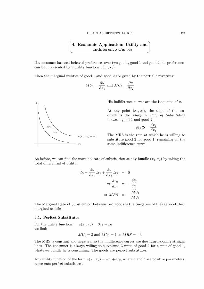
7. PARTIAL DIFFERENTIATION 127
✏�
��
4. Economic Application: Utility and
Indi↵erence Curves
If a consumer has well-behaved preferences over two goods, good 1 and good 2, his preferencescan be represented by a utility function u(x1, x2).
Then the marginal utilities of good 1 and good 2 are given by the partial derivatives:
MU1 =@u
@x1and MU2 =
@u
@x2
dx2
dx1
x1
u(x1, x2) = u0
x2
.
.........
.........
.........
.......
.................................
................................
..............................
.............................
...........................
..........................
........................
..
...........................
.............................
..............................
................................
................................. ..................................
.
.........................................
.......................................
.....................................
..................................
................................
..............................
......................
......
..........................
..
.............................
..............................
...............................
............................... ................................
His indi↵erence curves are the isoquants of u.
At any point (x1, x2), the slope of the iso-quant is the Marginal Rate of Substitutionbetween good 1 and good 2.
MRS =dx2
dx1
The MRS is the rate at which he is willing tosubstitute good 2 for good 1, remaining on thesame indi↵erence curve.
As before, we can find the marginal rate of substitution at any bundle (x1, x2) by taking thetotal di↵erential of utility:
du =@u
@x1dx1 +
@u
@x2dx2 = 0
)
dx2
dx1= �
@u
@x1
@u
@x2
) MRS = �
MU1
MU2
The Marginal Rate of Substitution between two goods is the (negative of the) ratio of theirmarginal utilities.
4.1. Perfect Substitutes
For the utility function: u(x1, x2) = 3x1 + x2
we find:
MU1 = 3 and MU2 = 1 so MRS = �3
The MRS is constant and negative, so the indi↵erence curves are downward-sloping straightlines. The consumer is always willing to substitute 3 units of good 2 for a unit of good 1,whatever bundle he is consuming. The goods are perfect substitutes.
Any utility function of the form u(x1, x2) = ax1+bx2, where a and b are positive parameters,represents perfect substitutes.

128 7. PARTIAL DIFFERENTIATION
4.2. Cobb-Douglas Utility
For the utility functionu(x1, x2) = x
a
1xb
2
where a and b are positive parameters, we find:
MU1 = ax
a�11 x
b
2 and MU2 = bx
a
1xb�12
) MRS = �
ax
a�11 x
b
2
bx
a
1xb�12
= �
ax2
bx1
From this expression we can see:
• The MRS is negative so the indi↵erence curves are downward-sloping.• As you move along an indi↵erence curve, increasing x1 and decreasing x2, the MRS
becomes less negative, so the indi↵erence curve becomes flatter. Hence the indi↵er-ence curves are convex (as in the diagram on the previous page).
4.3. Transforming the Utility Function
If a consumer has a preference ordering represented by the utility function u(x1, x2), and f(u)is a monotonic increasing function (that is, f 0(u) > 0 for all u) then v(x1, x2) = f(u(x1, x2))is a utility function representing the same preference ordering, because whenever a bundle(x1, x2) is preferred to (y1, y2):
u(x1, x2) > u(y1, y2) , f(u(x1, x2)) > f(u(y1, y2))
The two utility functions represent the same preferences, provided that we are only inter-ested in the consumer’s ordering of bundles, and don’t attach any significance to the utilitynumbers.
Examples 4.1: If a consumer has a Cobb-Douglas utility function:
u(x1, x2) = x
a
1xb
2
f(u) = lnu is a monotonic increasing function so his preferences can also be representedby
v(x1, x2) = ln⇣x
a
1xb
2
⌘= a lnx1 + b lnx2
Note that if we calculate the MRS for the function v we find:
MU1 =a
x1and MU2 =
b
x2so MRS = �
ax2
bx1
Although their marginal utilities are di↵erent, v has the same MRS as u.
Exercises 7.5: Utility and Indi↵erence curves
(1)(1) Find the MRS for each of the following utility functions, and hence determinewhether the indi↵erence curves are convex, concave, or straight:
(a) u = x
121 + x
122 (b) u = x
21 + x
22 (c) u = ln(x1 + x2)
(2) Prove that for any monotonic increasing function f(u), the utility functionv(x1, x2) = f(u(x1, x2)) has the same MRS as the utility function u.(Hint : Use the Chain Rule to di↵erentiate v.)
Further Reading and Exercises
• Jacques §5.2.• Varian “Intermediate Microeconomics” Chapter 4

7. PARTIAL DIFFERENTIATION 129
✏�
��
5. The Chain Rule and Implicit
Di↵erentiation
5.1. The Chain Rule for Functions of Several Variables
If z is a function of two variables, x and y, and both x and y depend on another variable, t(time, for example), then z also depends on t. We have:
If z = z(x, y), and x and y are functions of t, then:
dz
dt
=@z
@x
dx
dt
+@z
@y
dy
dt
Note the similarity of this rule to
• the Chain Rule for functions of one variable in Chapter 6, and• the formula for the Total Di↵erential in section 3.3
Examples 5.1: Suppose the aggregate output of a country is given by:
Y = AK
↵
L
�
where K is the capital stock, and L is the labour force. If the capital stock and the labourforce are each growing according to:
L(t) = L0ent and K(t) = K0e
mt
(i) What are the proportional growth rates of capital and labour?As in Chapter 6 we have:
dL
dt
= nL0ent = nL(t) and similarly for K(t)
So labour is growing at a constant proportional rate n, and capital is growing at con-stant proportional rate m.
(ii) What is the rate of growth of output?Applying the Chain Rule:
dY
dt
=@Y
@K
dK
dt
+@Y
@L
dL
dt
)
dY
dt
= ↵AK
↵�1L
�
⇥mK + �AK
↵
L
��1⇥ nL
= ↵mAK
↵
L
� + �nAK
↵
L
�
= (↵m+ �n)Y
So output grows at a constant proportional rate (↵m+ �n).
5.2. Implicit Di↵erentiation
The equation:x
2 + 2xy + y
3� 4 = 0
describes a relationship between x and y. If we plotted values of x and y satisfying thisequation, they would form a curve in (x, y) space. We cannot easily rearrange the equationto find y as an explicit function of x, but we can think of y as an implicit function of x, and

130 7. PARTIAL DIFFERENTIATION
ask how y changes when x changes – or in other words, what is dy
dx
? To answer this question,we can think of the left-hand side of the equation
x
2 + 2xy + y
3� 4 = 0
as a function of two variables, x and y. And in general, if we have any equation:
f(x, y) = 0
we can find the gradient of the relationship between x and y in exactly the same way as wefound the gradient of an isoquant in section 3.4, by totally di↵erentiating:
df =@f
@x
dx+@f
@y
dy = 0
)
@f
@y
dy = �
@f
@x
dx
)
dy
dx
= = �
@f
@x
@f
@y
Finding the gradient of y(x) when y is an implicit function of x is called implicit di↵eren-tiation. The method explained here, using the total derivative, is the same as the one inJacques. Anthony and Biggs use an alternative (but equivalent) method, applying the ChainRule of the previous section.
Examples 5.2: Implicit Di↵erentiation
(i) Find dy
dx
if x
2 + 5xy + y
3� 4 = 0
(2x+ 5y)dx+ (5x+ 3y2)dy = 0
(5x+ 3y2)dy = �(2x+ 5y)dx
dy
dx
= = �
2x+ 5y
5x+ 3y2
(ii) Find dq
dp
if q
2 + e
3p� pe
2q = 0
(2q � 2pe2q)dq + (3e3p � e
2q)dp = 0
(2q � 2pe2q)dq = (e2q � 3e3p)dp
dq
dp
= =e
2q� 3e3p
2(q � pe
2q)
Exercises 7.6: The Chain Rule and Implicit Di↵erentiation
(1)(1) If z(x, y) = 3x2 + 2y3, x = 2t + 1, and y = 4t � 2, use the chain rule to find dz
dt
when t = 2.
(2) If the aggregate production function is Y = K
13L
23 , what is the marginal product
of labour? If the labour force grows at a constant proportional rate n, and thecapital stock grows at constant proportial rate m, find the proportional growthrate of (a) output, Y and (b) the MPL.
(3) If xy2 + y � 2x = 0, finddy
dx
when y = 2.
Further Reading and Exercises
• Jacques §5.1• Anthony and Biggs §11.3, §12.1, §12.2 and §12.3.

7. PARTIAL DIFFERENTIATION 131
↵⌦
� 6. Comparative Statics
Examples 6.1:
(i) Suppose the inverse demand and supply functions for a good are:
p
d = a� q and p
s = bq + c where b > 0 and a > c > 0
How does the quantity sold change (a) if a increases (b) if b increases?
Putting p
d = p
s and solving for the equilibrium quantity: q
⇤ =a� c
1 + b
.
....................................................................................................................................................................................................
....................................................................................................................................................................................................
.
......................
......................
......................
......................
......................
......................
......................
......................
....
......................
......................
......................
......................
......................
......................
......................
......................
....
q
p
c
a p
s
p
d
We can answer the question by di↵erentiating with respectto the parameters:
@q
⇤
@a
=1
1 + b
> 0
This tells us that if a increases – that is, there is an upwardshift of the demand function – the equilibrium quantity willincrease. (You can, of course, see this from the diagram.)
Similarly@q
⇤
@b
< 0, so if the supply function gets steeper q⇤
decreases.
(ii) Suppose the inverse demand and supply functions for a good are:
p
d = a+ f(q) and p
s = g(q) where f
0(q) < 0 and g
0(q) > 0
How does the quantity sold change if a increases?
Here we don’t know much about the supply and demand functions, except that theyslope up and down in the usual way. The equilibrium quantity q
⇤ satisfies:
a+ f(q⇤) = g(q⇤)
We cannot solve explicitly for q⇤, but this equation defines it as an implicit function ofa. Hence we can use implicit di↵erentiation:
da+ f
0(q⇤)dq⇤ = g
0(q⇤)dq⇤ )
dq⇤
da
=1
g
0(q⇤)� f
0(q⇤)> 0
Again, this tells us that q⇤ increases when the demand function shifts up.
The process of using derivatives to find out how an equilibrium depends on the parametersis called comparative statics.
Exercises 7.7: If the labour supply and demand functions are
l
s = aw and l
d =k
w
where a and k are positive parameters:
(1)(1) What happens to the equilibrium wage and employment if k increases?
(2) What happens to the equilibrium wage and employment if a decreases?
Further Reading and Exercises
• Jacques §5.3 gives some macroeconomic applications of Comparative Statics.

132 7. PARTIAL DIFFERENTIATION
Solutions to Exercises in Chapter 7
Exercises 7.1:
(1) @f
@x
= 6x�y
4 @f
@y
= �4xy3
(2) @h
@x
= 2(x+ 1)(y + 2)@h
@y
= (x+ 1)2
(3) @g
@x
= 1xy
@g
@y
= �
lnx
y
2
Exercises 7.2:
(1) f
x
= 2x+ 3y, fy
= 3x,f
xx
= 2, fyy
= 0,f
yx
= f
xy
= 3.(2) g
p
= 2q2e2p+1,g
q
= 2qe2p+1 + r,g
r
= q,g
pp
= 4q2e2p+1,g
= 2e2p+1,g
rr
= 0,g
qp
= g
pq
= 4qe2p+1,g
rp
= g
pr
= 0,g
rq
= g
qr
= 1.(3) @z
@x
= 22x+3y > 0
@z
@y
= 32x+3y > 0
(4) f
x
= 6x(x2 + y
2 + z
2)2
f
xx
= 6(x2 + y
2 + z
2)2 +24x2(x2 + y
2 + z
2)= 6(x2 + y
2 + z
2)⇥ (5x2 + y
2 + z
2)f
xz
= 24xz(x2 + y
2 + z
2)(5) F
K
= ↵AK
↵�1L
�
F
L
= �AK
↵
L
��1
F
KL
= F
LK
= ↵�AK
↵�1L
��1
(6) u23 = 2, u12 = 0
Exercises 7.3:
(1) (a) @Q
@L
= 2L(K � 2)= 24
(b) @Q
@K
= L
2 = 9(c) It increases:
@
2Q
@L@K
= 2L > 0
(2) Y (�K,�L)
= (�12K
12 + �
12L
12 )2
= (�12 (K
12 + L
12 )2
= �(K12 + L
12 )2
= �Y (K,L)
F
K
= K
� 12 (K
12 + L
12 )
F
L
= L
� 12 (K
12 + L
12 )
) KF
K
+ LF
L
= (K12 + L
12 )2
(3) (a) ✏11 = �2, ✏12 = 1,⌘1 = 1
(b) x1(�p1,�p2,�pm)= �p2�m
�
2p
21
= p2m
p
21
If all prices dou-ble, but income dou-bles too, demandsshouldn’t change.
(4) p1@x1@p1
+p2@x1@p2
+m
@x1@m
= 0Dividing by x1 gives:✏11 + ✏12 + ⌘1 = 0
Exercises 7.4:
(1) �C = dC
dq
�q = 8⇥ 10= 80) C = £12000 +£80= £12080
(2) �Y = 3.4⇥�1 + 2⇥�1= �5.4
(3) (a) dz = 30x2y5dx+ 50x3y4dy
(b) df = 2x1dx1+ x3dx2 + x2dx3
� 10x4dx4(4) (4x3 + 2xy2)dx
+ 2x2ydy = 0
)
dy
dx
= �
4x3+2xy2
2x2y
= �
2x2+y
2
xy
When x = 1 and g = 10,
y = 3.Then dy
dx
= �
113
(5) MRTS = �
2KL+K
L
2+L
= �
K(2L+1)L(L+1)
Exercises 7.5:
(1) (a) MRS = �(x2x1)12
Convex(b) MRS = �(x1
x2)
Concave(c) MRS = �1
Straight(2) @v
@x1= f
0(u) @u
@x1and
@v
@x2= f
0(u) @u
@x2
so the ratio of the MUs isthe same for u and v.
Exercises 7.6:
(1) dz
dt
= 6x⇥ 2 + 6y2 ⇥ 4= 6⇥ 5⇥ 2+6⇥ 36⇥ 4 =924
(2) MPL = 23K
13L
� 13
(a) 13m+ 2
3n
(b) 13m�
13n
(3) When y = 2, x = �1.dy
dx
= 2�y
2
2xy+1 = 23
Exercises 7.7:
(1) In equilibrium, w =q
k
a
and l =p
ak.@w
@k
= 12pak
> 0 and@l
@k
= 12
pa
k
> 0so both w and l increasewhen k increases.
(2) @w
@a
= �
12
p
ka
� 32< 0 and
@l
@a
= 12
qk
a
> 0
so w increases and l de-creases when a decreases.
1This Version of Workbook Chapter 7: September 25, 2014

7. PARTIAL DIFFERENTIATION 133
⌥⌃ ⌅⇧Worksheet 7: Partial Di↵erentiation
Quick Questions
(1) Obtain the first-order partial derivatives of each of the following functions:
f (x, y) = 4x2y + 3xy3 + 6x; g (x, y) = e
2x+3y; h (x, y) =x+ y
x� y
.
(2) Show that the function
f (x, y) =p
xy +x
2
y
is homogeneous of degree 1. Find both partial derivatives and hence verify that itsatisfies Euler’s Theorem.
(3) A firm has production functionQ(K,L) = KL
2, and faces demand function P
d(Q) =120� 1.5Q.(a) Find the marginal products of labour and capital when L = 3 and K = 4.(b) Write down the firm’s revenue, R, as a function of output, Q, and find its
marginal revenue.(c) Hence, using the chain rule, find the marginal revenue product of labour when
L = 3 and K = 4.
(4) A consumer has a quasi-linear utility function u(x1, x2) = x
121 +x2. Find the marginal
utilities of both goods and the marginal rate of substitution. What does the MRStell us about the shape of the indi↵erence curves? Sketch the indi↵erence curves.
(5) For a firm with Cobb-Douglas production function Y (K,L) = aK
↵
L
� , show that themarginal rate of technical substitution depends on the capital-labour ratio. Showon a diagram what this means for the shape of the isoquants.
(6) The supply and demand functions in a market are
Q
s = kp
2 and Q
d = D(p)
where k is a positive constant and the demand function slopes down: D0(p) < 0.(a) Write down the equation satisfied by the equilibrium price.(b) Use implicit di↵erentiation to find how the price changes if k increases.
Longer Questions
(1) A consumer’s demand for good 1 depends on its own price, p1, the price of good 2,p2, and his income, y, according to the formula
x1 (p1, p2, y) =y
p1 +p
p1p2.
(a) Show that x1 (p1, p2, y) is homogeneous of degree zero. What is the economicinterpretation of this property?
(b) The own-price elasticity of demand is given by the formula
✏11 (p1, p2, y) =p1
x1
@x1
@p1.
Show that |✏11| is always less than 1.

134 7. PARTIAL DIFFERENTIATION
(2) Tony and Gordon have utility functions:
Tony : U
T
(x, y) = x
4y
2
Gordon : U
G
(x, y) = lnx+ 12 ln y
(a) Find their marginal utilities for both goods, and show that they both have thesame marginal rate of substitution.
(b) What is the equation of Tony’s indi↵erence curve corresponding to a utilitylevel of 16? Show that it is convex, and draw it.
(c) Does Gordon have the same indi↵erence curves? Explain carefully how theirindi↵erence curves are related.
(d) Show that Gordon has “diminishing marginal utility”, but Tony does not.(e) Do Tony and Gordon have the same preferences?
(3) Robinson Crusoe spends his 9 hour working day either fishing or looking for co-conuts. If he spends t hours fishing, and s hours looking for coconuts, he will catch
f(t) = t
12 fish, and collect c(s) = 2s
13 coconuts.
(a) If Crusoe’s utility function is U(f, c) = ln(f) + ln(c), show that the marginalrate at which he will substitute coconuts for fish is given by the expression:
MRS = �
c
f
(b) Show that production possibility frontier of the economy is:
f
2 +⇣c
2
⌘3= 9
(c) Find an expression for the marginal rate of transfomation between fish andcoconuts.
(d) Crusoe plans to spend 1 hour fishing, and the rest of his time collecting coconuts.If he adopts this plan:
(i) How many of each can he consume?(ii) What is his MRS?(iii) What is his MRT?(iv) Would you recommend that he should spend more or less time fishing?
Why? Draw a diagram to illustrate.(e) What would be the optimal allocation of his time?

CHAPTER 8
Unconstrained Optimisation Problems with One or MoreVariables
In Chapter 6 we used di↵erentiation to solve optimisation problems. Inthis chapter we look at more economic applications of this technique:profit maximisation in perfect competition and monopoly; andstrategic optimisation problems that arise in oligopoly or when thereare externalities. Then we show how to maximise or minimise afunction of more than one variable, and again look at applications.
—./—↵⌦
� 1. The Terminology of Optimisation
Suppose that an economic agent wants to choose some value y to maximise a function ⇧(y).For example, y might be the quantity of output and ⇧(y) the profit of a firm. From Chapters5 and 6 we know how to solve problems like this, by di↵erentiating.
The agent’s optimisation problem is:max
y
⇧(y)
⇧(y) is called the agent’s objective function - the thing he wants to optimise.
To solve the optimisation problem above, we can look for avalue of y that satisfies two conditions:
The first-order condition:d⇧dy
= 0
and the second-order condition:d
2⇧dy
2< 0
But remember that if we find a value of y satisfying these conditions it is not necessarily theoptimal choice, because the point may not be the global maximum of the function. Also,some functions may not have a global maximum, and some may have a maximum point forwhich the second derivative is zero, rather than negative. So it is always important to thinkabout the shape of the objective function.
An optimisation problem may involve minimising rather than maximising – for examplechoosing output to minimise average cost:
minq
AC(q)
The first- and second-order conditions are, of course, dAC
dq
= 0 and d
2AC
dq
2 > 0, respectively.135

136 8. UNCONSTRAINED OPTIMISATION PROBLEMS
⌥⌃
⌅⇧2. Profit Maximisation
Suppose a firm has revenue function R(y) and cost function C(y), where y is the the quantityof output that it produces. Its profit function is:
⇧(y) = R(y)� C(y)
The firm wants to choose its output to maximise profit. Its optimisation problem is:
maxy
⇧(y)
The first-order condition for profit maximisation is:d⇧dy
= R
0(y)� C
0(y) = 0
which is the familiar condition that marginal revenue equals marginal cost.
Examples 2.1: A monopolist has inverse demand function P (y) = 35�3y and cost functionC(y) = 50y + y
3� 12y
2.
(i) What is the profit function?
⇧(y) = yP (y)� C(y)= (35� 3y)y � (50y + y
3� 12y
2)= �y
3 + 9y
2� 15y
(ii) What is the optimal level of output?The first-order condition is:
d⇧dy
= �3y
2 + 18y � 15 = 0
There are two solutions: y = 1 or y = 5.Check the second-order condition:
d
2⇧dy
2= �6y + 18
When y = 1, d
2⇧dy
2 = 12 so this is a minimum point.
When y = 5, d
2⇧dy
2 = �12 so this is the optimal level of output.
(iii) What is the market price, and how much profit does the firm make?The firm chooses y = 5. From the market demand function the price is P (5) = 20.The profit is ⇧(5) = 25.
2.1. Perfect Competition
A firm operating in a perfectly competitive market is a price-taker. If p is the market price,its revenue function is R(y) = py and its profit function is:
⇧(y) = py � C(y)
Again, the firm’s optimisation problem is:
maxy
⇧(y)

8. UNCONSTRAINED OPTIMISATION PROBLEMS 137
The first-order condition (FOC) is:d⇧dy
= p� C
0(y) = 0
) p = C
0(y)
A competitive firm alway chooses output so that price = marginal cost.
y
p
. ........................................
......................
........................
..........................
.............................
.................................
....................................
.......................................
...........................................
..............................................
..................................................
.....................................................
........................................................
............................................................
.
.......................................
....................................
.................................
..............................
........................
...
........................
......................
......................
..................... ..................... .................... .................... ...........................................
.................................................
...........................
............................
..............................
.................................
....................................
.......................................
..........................................
.............................................
p = C
0(y)
AC(y)
•
E
p = C
0(y) is the inverse supply function for acompetitive firm.
Remember from Chapter 6 that the MC func-tion passes through the minimum point of theaverage cost function.
In the long-run, firms enter a competitive mar-ket until (for the marginal firm) profit is zero:
py � C(y) = 0
) p =C(y)
y
= AC(y)
Point E is the long-run equilibrium.
At point E: p = MC (the firm is profit-maximising) and p = AC (it is making zero-profit).
Examples 2.2: In a competitive market, all firms have cost-functions C(y) = y
2 + y + 4.The market demand function is Q = 112� 2p. Initially there are 40 firms.
(i) What is the market supply function?If the market price is p, each firm has profit function:
⇧(y) = py � (y2 + y + 4)
The firm chooses output to maximise profit. The FOC is:
p = 2y + 1
This is the firm’s inverse supply function. (The SOC is satisfied: d
2⇧dy
2 = �2.)The firm’s supply function is:
y =p� 1
2There are 40 firms, so total market supply is given by:
Q = 40y
) Q = 20(p� 1)
(ii) What is the market price and quantity in the short-run?Equating market demand and supply:
112� 2p = 20(p� 1) ) p = 6
Then from the demand function Q = 112� 2p = 100.The market price is 6, and the total quantity is 100.Since there are 40 firms, each firm produces 2.5 units of output.

138 8. UNCONSTRAINED OPTIMISATION PROBLEMS
(iii) How much profit do firms make in the short-run?
⇧(y) = py � (y2 + y + 4)
When p = 6 and y = 2.5, profit is 2.25.
(iv) What happens in the long-run?Since firms are making positive profits, more firms will enter. In the long-run, all firmswill produce at minimum average cost:
AC(y) = y + 1 +4y
dAC
dy
= 1�4y
2= 0
) y = 2 and AC = 5
So the long-run market price is p = 5, and every firm produces 2 units of output.At this price, market demand is: Q = 112� 2p = 102.Hence there will be 51 firms in the market.
2.2. Comparing Perfect Competition and Monopoly
For all firms the FOC for profit maximisation is marginal revenue = marginal cost :
R
0(y) = C
0(y)
For a competitive firm:
R(y) = py
) R
0(y) = p
Hence, at the optimal choice of output, price equals marginal cost:
p = C
0(y)
A monopolist faces a downward-sloping inverse demand function p(y) where p
0(y) < 0:
R(y) = p(y)y) R
0(y) = p(y) + p
0(y)y (Chain Rule)< p(y)
So marginal revenue is less than price.Hence, at the optimal choice of output, price is greater than marginal cost:
C
0(y) = R
0(y) < p(y)
Examples 2.3: Compare the price and marginal cost for the monopolist in Examples 2.1.
C(y) = 50y + y
3� 12y
2
) C
0(y) = 50 + 3y
2� 24y
We found that the optimal choice of output was y = 5 and the market price was P = 20.The marginal cost is C
0(5) = 5.

8. UNCONSTRAINED OPTIMISATION PROBLEMS 139
Exercises 8.1: Perfect Competition and Monopoly(1)(1) A monopolist has fixed cost F = 20 and constant marginal cost c = 4, and faces
demand function Q = 30� P/2.
(a) What is the inverse demand function?
(b) What is the cost function?
(c) What is the firm’s profit function?
(d) Find the firm’s optimal choice of output.
(e) Find the market price and show that it is greater than marginal cost.
(2) What is the supply function of a perfectly competitive firm with cost functionC(y) = 3y
2 + 2y + 4?
(3) What is the long-run equilibrium price in a competitive market where all firmshave cost function C(q) = 8q
2 + 128?
(4) In a competitive market the demand function is Q = 120/P . There are 40 identicalfirms, each with cost function C(q) = 2q
32 + 1. Find:
(a) The inverse supply function of each firm.
(b) The supply function of each firm.
(c) The market supply function.
(d) The market price and quantity.
Is the market in long-run equilibrium?
(5) A monopolist faces inverse demand function p = 720� 14q
3 + 193 q
2� 54q, and has
cost function C(q) = 540q. Show that the profit function has three stationarypoints: q = 3, q = 6, and q = 10. Classify these points. What level of outputshould the firm choose? Sketch the firm’s demand function, and the marginalrevenue and marginal cost functions.
Further Reading and Exercises• Jacques §4.6 and §4.7• Anthony & Biggs §§9.2, 9.3, 10.1 and 10.2• Varian Chapters 19-24

140 8. UNCONSTRAINED OPTIMISATION PROBLEMS
↵⌦
� 3. Strategic Optimisation Problems
In some economic problems an agent’s payo↵ (his profit or utility) depends on his own choicesand the choices of other agents. So the agent has to make a strategic decision: his optimalchoice depends on what he expects the other agents to do.
Suppose we have two agents. Agent 1’s payo↵ is ⇧1(y1, y2) and agent 2’s payo↵ is ⇧2(y1, y2).y1 is a choice made by agent 1, and y2 is a choice made by agent 2. Suppose agent 1 expectsagent 2 to choose y
e
2. Then his optimisation problem is:
maxy1
⇧1(y1, ye
2)
The first- and second-order conditions for this problem are:
@⇧1
@y1= 0 and
@
2⇧1
@y
21
< 0
Note that we use partial derivatives, because agent 1 treats y
e
2 as given - as a constant thathe cannot a↵ect. Similarly agent 2’s problem is:
maxy2
⇧2(ye
1, y2)
We can solve both of these problems and look for a pair of optimal choices y1 and y2 wherethe agents’ expectations are fulfilled: y1 = y
e
1 and y2 = y
e
2. This will be a Nash equilibrium,in which both agents make optimal choices given the choice of the other.
3.1. Oligopoly
When there are few firms in a market, the decisions of one firm a↵ect the profits of the others.We can model firms as choosing quantities or prices.
Examples 3.1: The Cournot Model: Simultaneous Quantity Setting
There are two firms in a market where the demand function is Q = 20� 12P . Each firm has
cost function C(q) = 4q + 5. The firms choose their quantities simultaneously.
(i) If firm 1 chooses quantity q1, and firm 2 chooses q2, what is the market price?
The inverse demand function is P = 40� 2Q. The total quantity is Q = q1 + q2.Hence the market price is:
P = 40� 2(q1 + q2)
(ii) What is firm 1’s profit, as a function of q1 and q2?
⇧1(q1, q2) = q1(40� 2(q1 + q2))� (4q1 + 5)= 36q1 � 2q
21 � 2q1q2 � 5
(iii) If firm 1 expects firm 2 to choose q
e
2, what is its optimal choice of output?
Firm 1’s optimisation problem is:
maxq1
⇧1(q1, qe
2) where ⇧1(q1, qe
2) = 36q1 � 2q
21 � 2q1q
e
2 � 5

8. UNCONSTRAINED OPTIMISATION PROBLEMS 141
The first-order condition is:@⇧1
@q1= 36� 4q1 � 2q
e
2 = 0
) q1 = 9� 12q
e
2
This is the firm’s reaction function. Note that @
2⇧1@q
21
= �4, so the second-order condi-tion is satisfied.
(iv) If firm 2 expects firm 1 to choose q
e
1, what is its optimal choice of output?In just the same way: q2 = 9� 1
2q
e
1
(v) How much does each firm produce in equilibrium?
In equilibrium, both firms’ expectations are fullfilled: q1 = q
e
1 and q2 = q
e
2. Hence:
q1 = 9� 12q2 and q2 = 9� 1
2q1
Solving this pair of simultaneous equations we find:
q1 = q2 = 6
(vi) How much profit does each firm make?
From the profit function above: ⇧1(6, 6) = 67. The profit for firm 2 is the same.
Examples 3.2: The Stackelberg Model
Suppose that, in the market of the previous example, with demand function Q = 20 � 12P
and cost functions C(q) = 4q + 5, firm 1 chooses its quantity first, and firm 2 observes firm1’s choice before choosing its own quantity.
(i) What is firm 2’s reaction function?
When firm 2 makes its choice, it already knows the value of q1. So its optimisationproblem is:
maxq2
⇧2(q1, q2) where ⇧2(q1, q2) = 36q2 � 2q
22 � 2q1q2 � 5
As in the previous example its reaction function is:
q2 = 9� 12q1
(ii) What is firm 1’s optimal choice?
As before, firm 1’s profit is: ⇧1(q1, q2) = 36q1 � 2q
21 � 2q1q2 � 5
but this time it knows that firm 2 will choose q2 = 9� 12q1.
So we can write the problem as
maxq1
36q1 � 2q
21 � 2q1(9� 1
2q1)� 5
Solving this problem we obtain q1 = 9.
(iii) How much output does each firm produce?
We know that firm 1 will choose q1 = 9. Therefore, from its reaction function, firm 2chooses q2 = 4.5.

142 8. UNCONSTRAINED OPTIMISATION PROBLEMS
3.2. Externalities
An externality occurs when the decision of one agent directly a↵ects the profit or utility ofanother. It usually causes ine�ciency, as the following example illustrates.
Examples 3.3: A mutual positive consumption externality
Two neighbours, A and B, each get pleasure u(R) = 24R
12 from the number of roses they can
see. If A has r
A
roses in her garden, and B has r
B
roses in his, then the number of roses thatA can see is R
A
= r
A
+ 12r
B
. Similarly B can see R
B
= r
B
+ 12r
A
. The cost of planting onerose is c = 2. Each chooses the number of roses to plant to maximise their own net utility,taking the other’s choice as given. Hence, for example, A’s optimisation problem is:
maxrA
u(RA
)� cr
A
where R
A
= r
A
+ 12r
B
(i) If A believes that B will choose r
e
B
, how many roses should she plant?
We can write A’s optimisation problem as:
maxrA
24(rA
+ 12r
e
B
)12� 2r
A
The first-order condition is:
12(rA
+ 12r
e
B
)�12 = 2
Rearranging we obtain:r
A
= 36� 12r
e
B
This is A’s reaction function to B’s choice. The second-derivative of the objective func-tion is: �6(r
A
+ 12r
e
B
)�32
< 0, so the second order-condition is satisfied.
(ii) If B believes that A will choose r
e
A
, how many roses should he plant?In just the same way,
r
B
= 36� 12r
e
A
(iii) How many will each plant in equilibrium?
In equilibrium, the expectations of each neighbour are fulfilled: r
A
= r
e
A
and r
B
= r
e
b
.We have a pair of simultaneous equations:
r
A
= 36� 12r
B
and r
B
= 36� 12r
A
Solving gives: r
A
= r
B
= 24
(iv) Suppose the neighbours could make an agreement that each will plant the same num-ber of roses, r. How many should they choose?
If r roses are planted by each, each of them will be able to see 32r, so each will ob-
tain net utility:24
�32r
� 12� 2r
Choosing r to maximise this, the first-order condition is:
18�
32r
�� 12 = 2
Solving, we find that each should plant r = 54 roses. This is an e�cient outcome,giving both neighbours higher net utility than when they optimise separately.

8. UNCONSTRAINED OPTIMISATION PROBLEMS 143
Exercises 8.2: A Strategic Optimisation ProblemTwo firms produce di↵erentiated products. Firm 1 produces good 1, for which the demandfunction is:
q1(p1, p2) = 10� 2p1 + p2
where p1 is the price of good 1 and p2 is the price of good 2. Similarly firm 2’s demandfunction is:
q2(p1, p2) = 10� 3p2 + p1
Both firms have constant unit costs c = 3. They each choose their own price, taking theother’s price as given.
(1)(1) Write down the profit function for each firm, as a function of the prices p1 and p2.
(2) If firm 1 expects firm 2 to choose p
e
2, what price will it choose?
(3) Similarly, find firm 2’s reaction function to firm 1’s price.
(4) What prices are chosen in equilibrium, and how much of each good is sold?
Further Reading and Exercises• Varian (6th Edition) Chapters 27, 28 and 33

144 8. UNCONSTRAINED OPTIMISATION PROBLEMS
✏�
��
4. Finding Maxima and Minima ofFunctions of Two Variables
For a function of two variables f(x, y) we can try to find out which pair of values, x and y,give the largest value for f . If we think of the function as a land surface in 3-dimensions,with f(x, y) representing the height of the land at map-coordinates (x, y), then a maximumpoint is the top of a hill, and a minimum point is the bottom of a valley. As for functions ofone variable, the gradient is zero at maximum and minimum points - whether you move inthe x-direction or the y-direction:
The first order conditions for a maximum or minimumpoint of f(x, y) are:
@f
@x
= 0 and@f
@y
= 0
The gradient may be zero at other points which are not maxima and minima - for exampleyou can imagine the three-dimensional equivalent of a point of inflexion, where on the side ofa hill the land momentarily flattens out but then the gradient increases again. There mightalso be a saddle point - like the point in the middle of a horse’s back which if you move in thedirection of the head or tail is a local minimum, but if you move sideways is a maximum point.
Having found a point that satisfies the first-order conditions (a stationary point) we can checkthe second-order conditions to see whether it is a maximum, a minimum, or something else.Writing the second-order partial derivatives as f
xx
= @
2f
@x
2 , f
xy
= @
2f
@x@y
etc:
Second-order conditions:A stationary point of the function f(x, y) is:
a maximum point if f
xx
< 0, f
yy
< 0 and f
xx
f
yy
� f
2xy
> 0a minimum point if f
xx
> 0, f
yy
> 0 and f
xx
f
yy
� f
2xy
> 0a saddle-point if f
xx
f
yy
� f
2xy
< 0
Why are the second-order conditions so complicated? If you think about a maximum pointyou can see that the gradient must be decreasing in the x- and y-directions, so we must havef
xx
< 0 and f
yy
< 0. But this is not enough - it is possible to imagine a stationary pointwhere if you walked North, South, East or West you would go down-hill, but if you walkedNorth-East you would go uphill. The condition f
xx
f
yy
� f
2xy
> 0 guarantees that the pointis a maximum in all directions.
Note that, as for functions of one variable, we find local optima by solving the first- andsecond-order conditions. We need to think about the shape of the whole function to decidewhether we have found the global optimum.
4.1. Functions of More Than Two Variables
Similarly, for a function of several variables f(x1, x2, . . . , xn
) the first-order conditions formaxima and minima are that all the first-order partial derivatives are zero: f1 = 0, f2 =0, . . . , f
n
= 0. The second-order conditions are beyond the scope of this Workbook.

8. UNCONSTRAINED OPTIMISATION PROBLEMS 145
Examples 4.1: Find and classify the stationary points of the following functions:
(i) f(x, y) = �x
2 + xy � 2y
2� 3x + 12y + 50
The first-order conditions are:
f
x
= �2x + y � 3 = 0 and f
y
= x� 4y + 12 = 0
Solving, there is one stationary point: x = 0, y = 3.Find the second-order partial derivatives:
f
xx
= �2 f
yy
= �4 f
xy
= 1
So at (0, 3) (and everywhere else, for this function):
f
xx
< 0 f
yy
< 0 f
xx
f
yy
� f
2xy
= 8� 1 > 0
Hence the function has a maximum point at (0, 3), and the maximum value is f(0, 3) =68.
(ii) g(x, y) = y
3� 12y + x
2e
y
The first-order conditions are:
g
x
= 2xe
y = 0 and g
y
= 3y
2� 12 + x
2e
y = 0
From the first of these, x = 0 (since e
y is positive for all values of y).Putting x = 0 in the second equation, and solving, gives y = ±2.So there are two stationary points, at (0, 2) and (0,�2).
To classify them, find the second-order partial derivatives:
g
xx
= 2e
y
g
yy
= 6y + x
2e
y
g
xy
= 2xe
y
At (0, 2), g
xx
> 0, g
yy
> 0 and g
xx
g
yy
� g
2xy
> 0.– This is a minimum point, and g(0, 2) = �16.At (0,�2), g
xx
g
yy
� g
2xy
< 0.– This is a saddle point, and g(0,�2) = 16.
Thinking about this function, we can see that there is no global maximum or mini-mum, because when x = 0, g(x, y)!1 as y !1 and g(x, y)! �1 as y ! �1.
Exercises 8.3: Finding Maxima and Minima of Functions of Two Variables(1)(1) Find and classify the stationary point of f(x, y) = x
2 + 4y
2 + 11y � 7x� xy
(2) Show that the function g(x, y) = e
xy + 3x
2 + xy � 12x� 4y has a minimum pointwhere y = 0.
(3) Find and classify the stationary points of h(x, y) = 3x
2� 12y � 2(x� 2y)3.
Hint: it is easier to solve this if you don’t multiply out the brackets.
Further Reading and Exercises• Jacques §5.4• Anthony & Biggs Chapter 13

146 8. UNCONSTRAINED OPTIMISATION PROBLEMS
✏�
��
5. Optimising Functions of TwoVariables: Economic Applications
5.1. Joint Products
Sometimes two di↵erent goods can be produced more cheaply together, by one firm, than bytwo separate firms – for example, if one good is a by-product of the production process ofanother.Examples 5.1: Suppose a firm produces two goods with joint cost function
C(q1, q2) = 2q
21 + q
22 � q1q2
The markets for both products are competitive, with prices p1 and p2.Find the firm’s supply functions for the two goods.
(i) The firm’s maximisation problem is:
maxq1,q2
⇧(q1, q2) where ⇧(q1, q2) = p1q1 + p2q2 � (2q
21 + q
22 � q1q2)
(ii) The first-order conditions are:
@⇧@q1
= p1 � 4q1 + q2 = 0 and@⇧@q2
= p2 � 2q2 + q1 = 0
(iii) The second-order partial derivatives are:
@
2⇧@q
21
= �4@
2⇧@q
22
= �2@
2⇧@q1@q2
= 1
So if we can find a stationary point, it must be a maximum.
(iv) Solving the first-order conditions for q1 and q2 gives:
q1 =2p1 + p2
7and q2 =
4p2 + p1
7These are the firm’s optimal choices of quantity, as functions of the prices: they arethe firm’s supply functions for the two products. Note that:
@q1
@p2> 0 and
@q2
@p1> 0
The goods are complements in production - when the price of one product goes up,more is produced of both.
5.2. Satiation
When modelling consumer preferences we usually assume that “more is always better” – theconsumer wants as much as possible of all goods. But in some cases “enough is enough”– theconsumer reaches a satiation point.Examples 5.2: A restaurant serving pizzas and chocolate cakes o↵ers “as much as you caneat for £10”. Your utility function is u(p, c) = 4 ln(p + c) � p �
13c
2. If you go there, howmany pizzas and cakes will you consume?

8. UNCONSTRAINED OPTIMISATION PROBLEMS 147
(i) Your maximisation problem is:
maxp,c
u(p, c)
(Note that the price does not a↵ect your choice – it is a sunk cost).
(ii) The first-order conditions are:
@u
@p
=4
p + c
� 1 = 0
@u
@c
=4
p + c
�
23c = 0
Solving: c = 112 and p = 21
2 .For the second-order conditions:
@
2u
@p
2= �
4(p + c)2
< 0 and@
2u
@c
2= �
4(p + c)2
�
23 < 0
@
2u
@c@p
= �4
(p + c)2)
@
2u
@p
2
@
2u
@c
2�
✓@
2u
@c@p
◆2
= 23
4(p + c)2
> 0
So this is a maximum; you will consume 212 pizzas and 11
2 cakes.
5.3. Price Discrimination
A monopolist who sells in two di↵erent markets, where there are no arbitrage opportunities(it is not possible for a third-party to buy in one market and then sell in the other), canusually raise profits by selling at di↵erent prices in the two markets. This is third-degree
price discrimination.
Examples 5.3: A car-manufacturer has cost function C(q) = 24q
12 , and can sell to its
domestic and foreign customers at di↵erent prices. It faces demand functions q
d
= 36p
�2d
inthe domestic market, and q
f
= 256p
�4f
in the foreign market.
(i) Find the price elasticity of demand in the two markets.
dq
d
dp
d
= �72p
�3d
)
p
d
q
d
dq
d
dp
d
=p
d
36p
�2d
⇥�72p
�3d
= �2
So the price elasticity of demand in the domestic market is -2, and similarly the foreignelasticity is -4.
(ii) Write down the firm’s profit as a function of the number of cars sold in each market.
The inverse demand functions for the two goods are: p
d
= 6q
� 12
d
and p
f
= 4q
� 14
f
. Henceprofit is:
⇧(qd
, q
f
) = p
d
q
d
+ p
f
q
f
� C(qd
+ q
f
)
= 6q
12d
+ 4q
34f
� 24(qd
+ q
f
)12

148 8. UNCONSTRAINED OPTIMISATION PROBLEMS
(iii) How many cars will be sold in each market?The first-order conditions are:
3q
� 12
d
= 12(qd
+ q
f
)�12 and 3q
� 14
f
= 12(qd
+ q
f
)�12
(Note that MR must be the same in both markets.)From these two equations:
3q
� 12
d
= 3q
� 14
f
) q
f
= q
2d
Substituting for q
f
in the first equation and solving:
q
� 12
d
= 4(qd
+ q
2d
)�12
) q
d
= 15, q
f
= 225
Checking the second-order conditions is messy, but it can be verified that this is amaximum.
(iv) Compare the domestic and foreign prices.Substituting the optimal quantities into the inverse demand functions:
p
d
=6p
15and p
f
=4p
15So the price is lower in the foreign market, where demand is more elastic.
Exercises 8.4: Economic Applications(1)(1) A firm producing two goods has cost function C(q1, q2) = q
21+2q2(q2�q1). Markets
for both goods are competitive and the prices are p1 = 5 and p2 = 8. Find theprofit-maximising quantities.
(2) Show that a consumer with utility function u(x, y) = 2ax�x
2 +2by� y
2 +xy hasa satiation point.
(3) A monopolist has cost function C(q) and can sell its product in two di↵erentmarkets, where the inverse demand functions are p1(q1) and p2(q2). Assumingthat the monopolist can price-discriminate, write down its maximisation problem.Hence show that the ratio of prices in the two markets satisfies:
p1
p2=
1� 1|✏2|
1� 1|✏1|
where ✏1 and ✏2 are the price elasticities of demand.
Further Reading and Exercises• Jacques §5.4• Anthony and Biggs §13.1 and §13.2

8. UNCONSTRAINED OPTIMISATION PROBLEMS 149
Solutions to Exercises in Chapter 8
Exercises 8.1:(1) (a) P = 60� 2Q
(b) C(Q) = 4Q + 20(c) ⇧ = 56Q� 2Q
2� 20
(d) ⇧0 = 56� 4Q = 0) Q = 14 and ⇧00 = �4
(e) P = 32, MC=4(2) y = p�2
6
(3) AC = 8Q + 128Q
so dAC
dQ
= 8� 128Q
2 = 0) Q = 4, P = AC = 64
(4) (a) P = 3q
12
(b) q = P
2
9
(c) Q = 40P
2
9
(d) 409 P
2 = 120P
) P = 3, Q = 40, q = 1Find minimum AC: AC = 2q
12 + 1
q
dAC
dQ
= q
� 12�
1q
2 ) q = 1, AC = 3.It is in LR equilibrium.
(5) ⇧ = 720q �
14q
4 + 193 q
3� 54q
2� 540q
⇧0 = 180� q
3 + 19q
2� 108q
q = 3 ) ⇧0 = 0 so this is a stationarypoint. Similarly for q = 6 and q = 10.⇧00 = �3q
2 + 38q � 108q = 3 ) ⇧00 = �21; q = 6 ) ⇧00 = 12;and q = 10) ⇧00 = �28.3 and 10 are maxima.q = 3) ⇧ = 204.75q = 10) ⇧ = 233.33q = 10 is the optimal choice.For sketch note that demand slopes down,but MR increases for some q.
Exercises 8.2:(1) ⇧1 = p1q1 � 3q1
= (p1 � 3)(10� 2p1 + p2)and similarly⇧2 = (p2 � 3)(10� 3p2 + p1)
(2) @⇧1@p1
= 16� 4p1 + p
e
2 ) p1 = 16+p
e2
4
(3) p2 = 19+p
e1
6(4) p1 = 5, p2 = 4, q1 = 4, q2 = 3
Exercises 8.3:
(1) f
x
= 2x� 7� y, f
y
= 8y + 11� x
One stationary point: x = 3, y = �1.f
xx
= 2, f
yy
= 8,fxy
= �1, ) minimum.(2) g
x
= ye
xy +6x+y�12, g
y
= xe
xy +x�4When y = 0, g
x
= 6x�12 and g
y
= 2x�4.So (2, 0) is a stationary point.g
xx
= y
2e
xy + 6, g
yy
= x
2e
xy
g
xy
= e
xy + xye
xy + 1. At (2,0): g
xx
= 6,g
yy
= 4, g
xy
= 2) minimum.
(3) h
x
= 6x� 6(x� 2y)2 = 0h
y
= �12 + 12(x� 2y)2 = 0From second equation (x� 2y)2 = 1So from first equation x = 1.Then (1� 2y)2 = 1) y = 0 or y = 1.Stationary points are: (1,0) and (1,1).h
xx
= 6� 12(x� 2y), h
yy
= �48(x� 2y),h
xy
= 24(x � 2y). At (1,0): h
xx
= �6,h
yy
= �48, h
xy
= 24: saddlepoint.At (1,1): h
xx
= 18, h
yy
= 48, h
xy
= �24:minimum.
Exercises 8.4:
(1) ⇧ = 5q1 + 8q2 � (q21 + 2q2(q2 � q1))
@⇧@q1
= 5� 2q1 + 2q2, @⇧@q2
= 8� 4q2 + 2q1
) q1 = 9, q2 = 6.5. SOCs: @
2⇧@q
21
= �2,@
2⇧@q
22
= �4, @
2⇧@q1@q2
= 2) max.
(2) @u
@x
= 2a� 2x + y, @u
@y
= 2b� 2y + x
) x = 4a+2b
3 , y = 2a+4b
3 .@
2u
@x
2 = �2, @
2u
@y
2 = �2 @
2u
@x@y
= 1) max.
(3) maxq1,q2 p1q1 + p2q2 � C(q1 + q2)
FOCs: p1 + p
01q1 = C
0(q1 + q2)and p2 + p
02q2 = C
0(q1 + q2)) p1 + p
01q1 = p2 + p
02q2
) p1
⇣1 + q1
p1
dp1dq1
⌘= p2
⇣1 + q2
p2
dp2dq2
⌘
) Result.
1This Version of Workbook Chapter 8: September 25, 2006

150 8. UNCONSTRAINED OPTIMISATION PROBLEMS
◆✓
⇣⌘
Worksheet 8: UnconstrainedOptimisation Problems with One or
More Variables
(1) In a competitive industry, all firms have cost functions C(q) = 32 + 2q
2
(a) Write down the profit function for an individual firm when the market price isP , and hence show that the firm’s supply curve is
q =P
4(b) Find the firm’s average cost function, and determine the price in long-run in-
dustry equilibrium.The market demand function is Q = 3000� 75P .(c) In the short-run there are 200 firms. Find the industry supply function, and
hence the equilibrium price, and the output and profits of each firm.(d) How many firms will there be in long-run equilibrium?Suppose that a trade association could limit the number of firms entering the indus-try.(e) Find the equilibrium price and quantity, in terms of the number of firms, n.(f) What upper limit would the trade association set if it wanted to maximise in-
dustry revenue?
(2) Find and classify the stationary points of the function: f (x, y) = x
3 + y
3� 3x� 3y
(3) Two competing toothpastes are produced by a monopolist. Brand X costs 9 penceper tube to produce and sells at P
X
, with demand (in hundreds/day) given by:X = 2 (P
Y
� P
X
) + 4. Brand Y costs 12 pence per tube to produce and sells at P
Y
pence, with demand given by: Y = 0.25P
X
� 2.5P
Y
+ 52. What price should shecharge for each brand if she wishes to maximize joint profits?
(4) A firm’s production function is given by
Q = 2L
12 + 3K
12
where Q,L and K denote the number of units of output, labour and capital. Labourcosts are £2 per unit, capital costs are £1 per unit, and output sells at £8 per unit.(a) What is the firm’s profit function?(b) Find the maximum profit and the values of L and K at which it is achieved.
(5) Suppose there are two firms, firm 1 which sells product X, and firm 2 which sellsproduct Y. The markets for X and Y are related, and the inverse demand curves forX and Y are
p
X = 15� 2x� y, andp
Y = 20� x� 2y
respectively. Firm 1 has total costs of 3x and firm 2 has total costs of 2y.
(a) Are X and Y substitutes or complements?(b) If the two firms are in Cournot competition (i.e. each maximizes its own profits
assuming the output of the other is fixed), how much should each produce?

8. UNCONSTRAINED OPTIMISATION PROBLEMS 151
(6) Two workers work together as a team. If worker i puts in e↵ort e
i
, their total outputis y = A ln(1 + e1 + e2). Their pay depends on their output: if they produce y, eachreceives w = w0 + ky. A, w0 and k are positive constants. Each of them chooses hisown e↵ort level to maximise his own utility, which is given by:
u
i
= w � e
i
(a) Write worker 1’s utility as a function of his own and worker 2’s e↵ort.(b) If worker 1 expects worker 2 to exert e↵ort e2, what is his optimal choice of
e↵ort?(c) How much e↵ort does each exert in a symmetric equilibrium?(d) How could the two workers obtain higher utility?
(7) Two firms sell an identical good. For both firms the unit cost of supplying that goodis c. Suppose that the quantity demanded of the good, q, is dependent on its price,p, according to the formula q = 100� 20p.
(a) Assuming firm 2 is supplying q2 units of the good to the market, how manyunits of the good should firm 1 supply to maximize its profits? Express youranswer in terms of c and q2.
(b) Find, in terms of c, the quantity that each firm will supply so that it is maxi-mizing its profit given the quantity supplied by the other firm; in other words,find the Cournot equilibrium supplies of the two firms. What will be the marketprice of the good?
(c) Suppose that these two firms are in fact retailers who purchase their productfrom a manufacturer at the price c. This manufacturer faces the cost function
C (q) = 20 + q +140
q
2,
where q is the output level. Assuming that the manufacturer knows that theretail market for his good has a Cournot equilibrium outcome, at what priceshould he supply the good in order to maximize his profits?