The Mathematical Representation of the Arrow of Time (2012)

Meir Hemmo and Orly Shenker

The Mathematical Representation of the Arrow of Time

1. Introduction

1.1. The Direction of Time

Hans Reichenbach opens his book The Direction of Time with a chapter on “the emotive significance of time.” He writes:

The problem of time has always baffled the human mind. Not only the events of the external world but even all of our subjective experiences occur in time. ... What we experience in one moment, glides, in the next moment, into the past. There it remains forever, irretrievable, exempt from further change. ... Our emotional response to the flow of time is largely determined by the irresistibility of its passing away. ... We cannot stop it; we cannot turn it back. ... [and we know that] the end of all this ... is death. ... If we could stop time, we could escape death. ... The fear of death is thus transformed into a fear of time. ... Dissatisfied emotion has frequently been projected into logic. ... The fear of death has greatly influenced the logical analysis which philosophers have given to the problem of time. The belief that they have discovered paradoxes in the flow of time is called a ‘projection’ in modern psychological terminology. It functions as a defense mechanism; the paradoxes are intended to discredit physical laws that have aroused deeply rooted emotional antagonism. (Reichenbach 1956, 2–3)

Reichenbach’s words may create the impression that while physics tells us clear things about time, philosophers resist its discoveries. It is true, of course, that philosophers have always been aware of the difficulty to understand the notion of time. The words of Saint Augustine, who studies time in his Confessions, are as relevant today as they have been in the 4th century:

What, then, is time? If no one asks me, I know what it is. If I wish to explain it to him who asks me, I don’t know. (Book 11, chap. 14)

Often, scientists give the impression that their understanding of time has advanced considerably since the time of Saint Augustine. One example

167© Iyyun • The Jerusalem Philosophical Quarterly 61 (January–July 2012): 167–192

168 Meir Hemmo and Orly Shenker

is Isaac Newton, who begins the Principia (1687) by saying, in the first scholium:

I do not define time, space, place, and motion, as being well known to all.

He goes on to remark that the “common people” entertain some “prejudices” about time that must be removed, and then he turns to remove these prejudices in a brief comment on the notion of time. His brief comment reveals how far from the truth was the above sentence, how time is anything but “well known to all”: Newton’s comment in the scholium opened a debate that is still going on today, concerning the absolute versus relational nature of time.

Indeed, while science has advanced our understanding of certain aspects of time, other aspects of time remain as little understood as ever. In particular, despite the impression one may sometimes get from the literature, the directionality of time is a phenomenon for which physics has no explanation. It is this aspect of time on which we shall focus in this paper.

One often hears that statistical mechanics provides a satisfactory account of the arrow of time. But this is wrong: Statistical mechanics does not provide an arrow of time, and doesn’t even fully account for the direction in which thermodynamic process evolve in time;1 rather, it assumes a direction of time as well as a direction in time.2 The other theories of physics assume the arrow of time as well. The special theory of relativity assumes a direction of time in the same way that classical mechanics does, as we discuss below. In general relativity some solutions of Einstein’s field equations are such that the spacetime manifold turns out to be globally time orientable, and some are not. In the first class of solutions the theory assumes a direction of time in the same sense that we shall discuss below in the context of classical mechanics. In the second class of solutions, where the manifold is not globally time orientable, the direction of time is assumed locally. Cosmology is an application of the general theory of relativity together with observational data such as the red shift. As such it cannot give an arrow of time beyond that of general relativity. Similarly, thermodynamics is an application of statistical mechanics, together with observational data concerning the behavior of thermodynamic systems. As such it cannot give

1 The important distinction between an arrow of time and an evolution in time will be clarified below.2 See Albert 2000, chap. 4; Hemmo and Shenker 2012, chaps. 7 and 10.

The Mathematical Representation of the Arrow of Time 169

an arrow of time beyond that of mechanics. In quantum mechanics time is a parameter but the notion of velocity is somewhat different. Although it seems to us that our conclusion concerning the direction of time will hold also in quantum mechanics, the argument should be different, and therefore we do not undertake it here.3

In view of the scientific and philosophical literature on this topic until today, we think we can safely say that nobody understands the arrow of time.4

1.2. The Mathematical Language of Physics

Newton’s Principia contains not only general comments concerning time such as the one quoted above, but also mathematical physics; and here Newton has an opportunity to express some of his ideas about time in the language of mathematics. Newton begins his preface to the first edition of the Principia with the following sentence:

Since the ancients esteemed the science of mechanics of greatest importance in the investigation of natural things, and the moderns, rejecting substantial forms and occult qualities, have endeavored to subject the phenomena of nature to the laws of mathematics, I have in this treatise cultivated mathematics as far as it relates to philosophy.

The notions that Newton uses here, such as mechanics, mathematics, and philosophy, may not have the meaning we would give these terms today.5 But we think it is, on the whole, correct to say, that an important aspect of Newton’s work was to develop mathematics, and to use this mathematics as part of a theory which we would today call physics. Newton emphasizes that he cultivates mathematics “as far as it relates to philosophy,” and the verb ‘cultivate’ here is very appropriate, for Newton both develops the mathematics and uses it for growing the physical crops.

Since—according to Newton—the notion of time is “well known to all,” it is interesting to see how this notion is described by the mathematics

3 Von Neumann (1932, chap. 5) attempted to derive the direction of time of the measurement process from the Second Law of thermodynamics. See Hemmo and Shenker (2006) for the extent in which he succeeded. Perhaps a new theory of quantum gravity will provide an arrow of time. 4 This, of course, is a paraphrase on Richard Feynman’s saying “I think I can safely say that nobody understands quantum mechanics” (Feynman 1965, 129). 5 To the extent that we can specify their meaning at all.


which he “cultivated.” Of course, by asking this question we make the non-trivial assumption, that mathematics is an acceptable way of describing physical ideas. That this assumption is not trivial is expressed in the famous words of Eugene Wigner in his paper “The Unreasonable Effectiveness of Mathematics in the Natural Sciences”:

The miracle of the appropriateness of the language of mathematics for the formulation of the laws of physics is a wonderful gift which we neither understand nor deserve. We should be grateful for it and hope that it will remain valid in future research and that it will extend, for better or for worse, to our pleasure, even though perhaps also to our bafflement, to wide branches of learning. (Wigner 1960, 237)

In what sense do we say that mathematics is applicable in the natural sciences, and how should we examine whether a particular case (such as the one discussed here, namely, the directionality of time) is properly captured by the mathematics of a given theory (here, classical mechanics)?

Generally speaking, the idea that mathematics is applicable in science means that it is possible to express statements about the world using mathematical expressions, and that once these expressions are given, mathematical manipulations can be applied in order to derive predictions and other insights about the world. 6 Of course, the constraint of logical validity entails that we can never get more insights out of the mathematical expressions, concerning the world, than we have originally put into them when they were formulated.7 Nevertheless, the mathematical formulation sometimes makes it easy to see and make explicit ideas put into it implicitly.

But then the question is, whether we put into the mathematics all and only the ideas we intended to, or at least ideas to which we don’t object. With respect to the mathematical representation of the arrow of time in classical mechanics, this leads to questions such as: Does the notion of the direction of time, which appears in the mathematical expressions of classical mechanics, include all and only the aspects of the direction of time that we take to be true of the world? Or are our mathematical expressions isomorphic to only some

6 We are not committed to realism here, and statements about ‘the world’ can be understood in any realist or anti-realist way the reader prefers.7 Contra the impression expressed by Hertz, who wrote: “One cannot escape the feeling that these mathematical formulae have an independent existence and intelligence of their own, that they are wiser than we are, wiser even than their discoverers, that we can get more out of them than was originally put into them,” quoted in Steiner (1998), 13.


aspects of the directionality of time, while leaving out others? Or—worse—can it be that the mathematics that we use tells us things about the arrow of time that are simply wrong, that is, things that are unintended artifacts of the mathematical apparatus?

Mark Steiner, in his book, The Applicability of Mathematics as a Philosophical Problem (1998, 25), deals with what he calls ‘descriptive applicability’, which is the appropriateness of specific mathematical concepts in describing and lawfully predicting physical phenomena. A central criterion for appropriateness in this context is associated with isomorphism between the mathematical structure in question and the structure of the way in which the physical magnitude allegedly behaves. In the cases where such an isomorphism is found, the descriptive applicability of a mathematical concept is reasonable and not mysterious; in those cases, “Where the [physical] property holds, the mathematical concept is there applicable, and vice versa” (1998, 35).

1.3. The Mathematical Expression of Time’s Arrow

Is this criterion satisfied by the mathematical representation of time in classical mechanics? Two options come to mind. One option is that (as Newton writes) the notion of time is “well known to all,” and so suitable mathematics should be found that is isomorphic in some sense to the main properties associated with this well-known notion. The primacy of the “well-known” notion of time means that should the mathematics turn out not to fit the pre-theoretic notion of time, the mathematical apparatus ought to be replaced. The other option is that the mathematics gains conceptual primacy: once it is chosen, it should be taken as fully expressing the entire notion of time, and therefore the properties of the notion of time should be deduced from the mathematics. It turns out that, as we will see later, with respect to the arrow of time in classical mechanics, the distinction between the two options is not always clear.

2. The Minimum Problem

Reichenbach, in the quotation cited earlier, focuses on one aspect of our temporal experience, namely, the feeling that the evolution of events has a direction. Reichenbach’s words may create the impression that the laws of


physics describe a world in which the events flow forward in time, towards the inevitable event of death; and that philosophers distort our understanding of this phenomenon, with the intention of discrediting the unpleasant picture it implies. But the truth of the matter is just the opposite: the fundamental theories of physics don’t provide us with any account of the phenomenon of the flow of time or of the directedness of time. They provide no explanation of this salient aspect of our experience; they hardly even describe it. By contrast, the philosophical literature is replete with discussions of this phenomenon, and Reichenbach’s book, The Direction of Time, is one of them.

We will later describe in what sense exactly the theories of physics lack temporal directionality. But first we wish to describe one result of this lack of time direction in these theories, in order to convince the reader that there is a serious problem here. The problem we will describe, very briefly, is called the minimum problem (or sometimes the parity of reasoning problem).

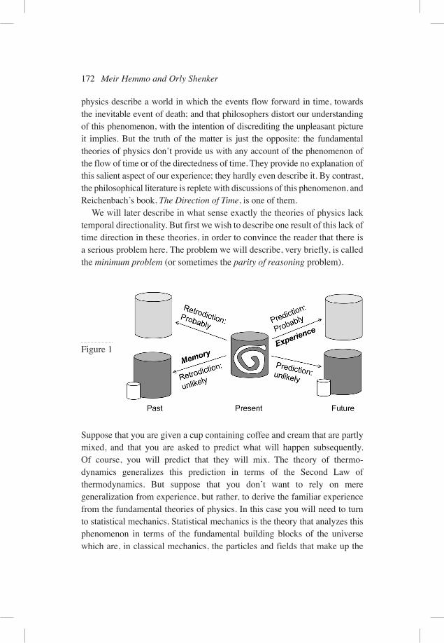
Suppose that you are given a cup containing coffee and cream that are partly mixed, and that you are asked to predict what will happen subsequently. Of course, you will predict that they will mix. The theory of thermodynamics generalizes this prediction in terms of the Second Law of thermodynamics. But suppose that you don’t want to rely on mere generalization from experience, but rather, to derive the familiar experience from the fundamental theories of physics. In this case you will need to turn to statistical mechanics. Statistical mechanics is the theory that analyzes this phenomenon in terms of the fundamental building blocks of the universe which are, in classical mechanics, the particles and fields that make up the

Figure 1


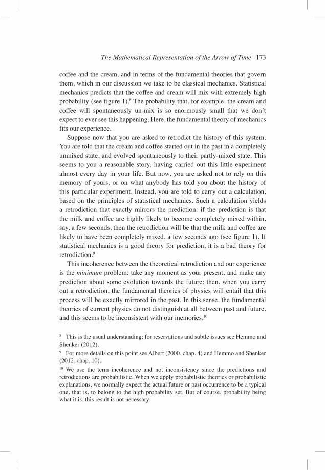
coffee and the cream, and in terms of the fundamental theories that govern them, which in our discussion we take to be classical mechanics. Statistical mechanics predicts that the coffee and cream will mix with extremely high probability (see figure 1).8 The probability that, for example, the cream and coffee will spontaneously un-mix is so enormously small that we don’t expect to ever see this happening. Here, the fundamental theory of mechanics fits our experience.

Suppose now that you are asked to retrodict the history of this system. You are told that the cream and coffee started out in the past in a completely unmixed state, and evolved spontaneously to their partly-mixed state. This seems to you a reasonable story, having carried out this little experiment almost every day in your life. But now, you are asked not to rely on this memory of yours, or on what anybody has told you about the history of this particular experiment. Instead, you are told to carry out a calculation, based on the principles of statistical mechanics. Such a calculation yields a retrodiction that exactly mirrors the prediction: if the prediction is that the milk and coffee are highly likely to become completely mixed within, say, a few seconds, then the retrodiction will be that the milk and coffee are likely to have been completely mixed, a few seconds ago (see figure 1). If statistical mechanics is a good theory for prediction, it is a bad theory for retrodiction.9

This incoherence between the theoretical retrodiction and our experience is the minimum problem: take any moment as your present; and make any prediction about some evolution towards the future; then, when you carry out a retrodiction, the fundamental theories of physics will entail that this process will be exactly mirrored in the past. In this sense, the fundamental theories of current physics do not distinguish at all between past and future, and this seems to be inconsistent with our memories.10

8 This is the usual understanding; for reservations and subtle issues see Hemmo and Shenker (2012).9 For more details on this point see Albert (2000, chap. 4) and Hemmo and Shenker (2012, chap. 10).10 We use the term incoherence and not inconsistency since the predictions and retrodictions are probabilistic. When we apply probabilistic theories or probabilistic explanations, we normally expect the actual future or past occurrence to be a typical one, that is, to belong to the high probability set. But of course, probability being what it is, this result is not necessary.


Astonishingly, the only available solution for the minimum problem is to assume bluntly that as a matter of fact—despite the probabilistic claims—the past was as we remember it. This is called the Past Hypothesis, and was expressed by Richard Feynman as follows: “I think it necessary to add to the physical laws the hypothesis that in the past the universe was more ordered, in the technical sense, than it is today” (1967, 116).11 (In Feynman’s terms, un-mixed coffee and cream are in a more ordered state, in the technical sense of the term, than mixed coffee and cream.) Forget for a moment the ad-hoc flavor of this idea; this flavor can be dealt with, in a way that we will not discuss here.12

The problem we would like to focus on is this: where in time—in what direction of time—is the past that Feynman is talking about? If the fundamental theories do not distinguish between past and future, how can we make the Past Hypothesis part of the theory? How can we express this hypothesis in terms of the theory of classical mechanics?

In order to make sense of the Past Hypothesis, there must be a way of breaking the symmetry between past and future in classical mechanics. This symmetry breaking can then be used to express, and then maybe explain, the asymmetry in time of our experience. We now turn to ask whether this can be done in a way that preserves the main ideas and achievements of classical mechanics.

In a nutshell, our claim will be this. The current mathematical representation of the world in classical mechanics is incomplete, since it lacks a direction of time, which is necessary to make the theory of classical mechanics well defined. That is, some internal aspects of the theory require bringing in a direction of time. This can be done either mathematically (in ways that we will mention below) or non-mathematically, but in either case this will be an addition to our current theories, something that they don’t include in their standard formulation as it stands today.

The plan of the rest of the paper is to explain why a direction of time is necessary in the theory, in what sense it is lacking, and how it can be brought into the theory.

11 See Albert (2000, chap. 4) for a variation on this idea.12 See Hemmo and Shenker (2012, chap. 10).


3. The Problem of Ambiguous Velocity

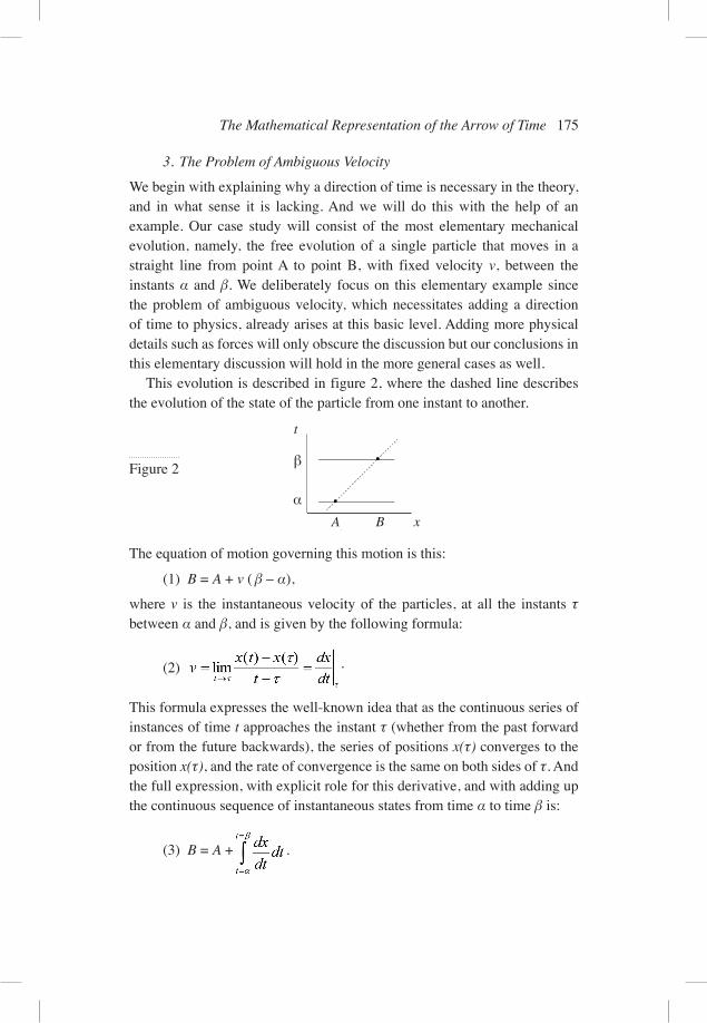
We begin with explaining why a direction of time is necessary in the theory, and in what sense it is lacking. And we will do this with the help of an example. Our case study will consist of the most elementary mechanical evolution, namely, the free evolution of a single particle that moves in a straight line from point A to point B, with fixed velocity v, between the instants α and β. We deliberately focus on this elementary example since the problem of ambiguous velocity, which necessitates adding a direction of time to physics, already arises at this basic level. Adding more physical details such as forces will only obscure the discussion but our conclusions in this elementary discussion will hold in the more general cases as well.

This evolution is described in figure 2, where the dashed line describes the evolution of the state of the particle from one instant to another.

Figure 2

α

β

t

xBA

The equation of motion governing this motion is this:

(1) B = A + v ( β – α),

where v is the instantaneous velocity of the particles, at all the instants τ between α and β, and is given by the following formula:

(2) .

This formula expresses the well-known idea that as the continuous series of instances of time t approaches the instant τ (whether from the past forward or from the future backwards), the series of positions x(τ) converges to the position x(τ), and the rate of convergence is the same on both sides of τ. And the full expression, with explicit role for this derivative, and with adding up the continuous sequence of instantaneous states from time α to time β is:

(3) B = A + .


What do these equations tell us about time? A useful way to think about this question is to consider the boring film that shows our particle that starts out in position A at time α and ends up in position B at time β. In the old days, this film would consist of a sequence of still frames on celluloid. This sequence of frames provides a convenient metaphor for the description of mechanical evolutions. On this metaphor, the mechanical picture of the world may be described in terms of time slices, analogous to frames of a film: each time-slice contains the position of the particle at that instant, as do the film frames. The continuous sequence of time-slices makes up the history of the universe.

But there are important dis-analogies between movie frames and the time slices that make up the mechanical history of the world. One dis-analogy is that the frames are discrete and therefore quite independent: if we take one frame out of the film, we can replace it with a variety of other frames, all of which will be consistent with the rest of the film. In mechanics, by contrast, the sequence of time-slices is continuous, and the positions of the particle converge everywhere in a way that determines a unique instantaneous speed13 of the particle at all times.14

But, the continuous sequence of time-slices (which determines the speed of the particle uniquely) still leaves some ambiguity with respect to the velocity of the particle. To see why, consider again expression (2) above, which describes the instantaneous velocity at all the instants τ between α and β.15 In fact, expression (2) determines only the magnitude of the velocity

13 Speed, not velocity; see below.14 The assumption that the motion of our particle, and mechanical motions in general, are smooth, is not necessary in any sense, nor entailed by the laws of mechanics, but it reflects our contingent experience. The equations of motion of classical mechanics are such that the instantaneous position and instantaneous velocity of a system, together, determine uniquely its positions at all other times; but this does not entail that a given system actually has an instantaneous velocity at all times. For a discussion of determinism in classical mechanics see Earman (1986).15 The notion of instantaneous velocity is notoriously problematic. Although the concept of instantaneous velocity is mathematically well defined in continuous space and time, its physical significance is questionable, since in order to measure velocity one needs to measures position in at least two instances. This problem is known since Zeno’s arrow paradox. Russell’s suggestion that instantaneous velocity is not part of the ontology runs into the problem of explaining what, exactly, is the aspect of the ontology which has the role of initial conditions that determine a system’s evolution (see discussion in Arntzenius 2000). In this paper we address a problem concerning


along each spatial direction, but the sign of this velocity (that is, the direction of the velocity) is not fully given by (2) alone. In order to read off from (2) a unique description of the velocity of a particle at τ we need to supply two additional pieces of information: one determines the counterpart in physical space of the expression at the numerator x(t)–x(τ), and the other piece of information is about the counterpart in physical time of the expression at the denominator, t–τ.

Normally, supplying these two pieces of information is taken to be an easy task: the direction of the difference between two positions can be fixed by some convenient convention such that, for example, if position B is to the right of position A, relative to a given reference point of view, then the number B is set to be greater than the number A. And the difference between two instances of time can be fixed such that, for example, if the instant β is later than the instant α then the number β is set to be greater than the number α.

However, there is a significant difference between the ways in which these two conventions are determined. The spatial relation of “to the right of” holds between two positions, if these positions stand in a certain relation relative to a privileged point, which is the point of view of the observer, called “here,” which is defined at every instant for every observer. The “here” position by itself does not suffice in order to determine the relation of “to the right of”: given the information concerning the location of “here,” the observer needs some non trivial additional information, namely, some convention,16 in order to be able to determine the “to the right of” relation uniquely.

The case of time is different. Any observer is able to report to any other observer which of any two events is later than the other (in the first observer’s rest frame), without using any convention to determine the direction of “later than.”17 And given the privileged instant of the present, the “now” (any “now”),

instantaneous velocity, which is different from and additional to the set of problems which followed the attempts to deal with Zeno’s paradox: the problem we address concerns the connection between instantaneous velocity and the direction of time.16 The violation of the postulated charge-parity (CP) symmetry is an interesting exception, discovered as a surprising fact, not an outcome of some fundamental principle, nor as a matter of convention. We don’t address it here.17 At least locally. If the spacetime manifold is not globally temporally orientable, a motion toward the future may be also a motion toward the past, e.g., in the so-called rotating universe solution in general relativity.


an observer is able to determine whether another instant is earlier or later than “now,” without needing any additional information (again, in the observer’s rest frame).18 In this sense it appears that, unlike the relation of “to the right of,” the relation of “later than” is not conventional; our experience is time directed but not space directed. This unique determination of the time direction is used in order to determine the sign of the denominator t–τ uniquely.

However, the way in which the time directedness of our experience enters the theory in the denominator of (2) is not via the mathematical aspect of the usual formulation of classical mechanics. In this sense, there is no mathematical representation of the arrow of time in classical mechanics. This fact brings to mind two questions: one question is (i) whether adding an arrow of time to classical mechanics is needed at all; and in case the answer to the first question is in the affirmative, the second question is (ii) in what way can this be done, and in particular, if this aim is to be achieved through the mathematics of the theory, how can one alter the usual mathematical formulation of classical mechanics in order to add such a representation.

Our answer to (i) is that adding a direction of time to the theory is absolutely necessary, for otherwise velocity is not well defined.19 The claim that we seem to do quite well without such an addition, and therefore don’t need it, is simply wrong: for we do add an arrow of time to the theory, but we do it implicitly, and not via the standard mathematical formalism or otherwise explicit aspect of the theory. The very fact that we know where the future is and that we use well-defined velocities is an outcome of this implicit assumption. In this paper our aim is to point out this fact, and then ask whether one should simply acknowledge and maybe explicate it, or whether one should aim to change the structure of the theory in order to incorporate the assumption of an arrow of time into the mathematics of the theory. We stress that the need to add a direction of time stems from conceptual consideration concerning the notion of velocity; it does not arise

18 Note that here we do not consider the question of the privileged status of the “now” in the context of the discussion about the view called presentism in the philosophy of time. Everything we said above holds no matter how one defines what Putnum (1967) calls the R relation,19 That is, adding an arrow is necessary, whether one is a relationist or an absolutist with respect to time.


from empirical considerations (the latter are relevant in statistical mechanics in the context of the Past Hypothesis; see section 2).

As to (ii), our answer is that adding an arrow of time to classical mechanics can be done either by changing the mathematics of the theory, or non-mathematically. The non-mathematical solution is the one used in the usual way of thinking about classical mechanics, and we analyze below in more detail the nature of this extra-mathematical assumption. As to the mathematical option, one can think of ways of changing the usual mathematical formulation of the theory in order to add a direction of time, e.g., by adding a locally time orientable manifold; however such a change may have implications that ought to be examined carefully.

Let us now examine in more detail the way in which the direction of time is added, implicitly and non-mathematically, to the usual way of for-mulating classical mechanics. As we said, we do add such a direction in such a way, and we do it necessarily, for otherwise we wouldn’t have well-defined velocities.

The lack of a mathematical representation of the direction of time in the usual formulation of classical mechanics is expressed by the fact that while x is a vector, t is a scalar. We can, of course, name instants in a convenient way by using a series of numbers which increases towards the future, but these names will indicate a direction only if we assume, or take for granted, something comparable to a unit vector of time, relative to which the names of instants are organized. This direction isn’t part of the mathematics of classical mechanics in the usual way of thinking about it. Although it isn’t part of the explicit mathematics of the theory, it is an implicit part of it, since we assume a direction of time whenever we ascribe a directed velocity to a particle. Without this assumption, as we said, the instantaneous velocity of our particle would be ambiguous: it could be any one of two velocities. And so whenever we take it that the velocity is well defined, we tacitly assume a direction of time.20

Since an assumption about the direction of time goes into ascribing a well-defined velocity to a particle, and since instantaneous velocity is part of the instantaneous mechanical state of a particle, which we plug into the equations of motion in order to predict or retrodict the system’s evolution, it turns out that the direction of time, which is implied whenever we ascribe

20 This holds even if the spacetime manifold is not globally temporally orientable.


instantaneous velocity to a system, is part of the instantaneous mechanical state of a particle.21

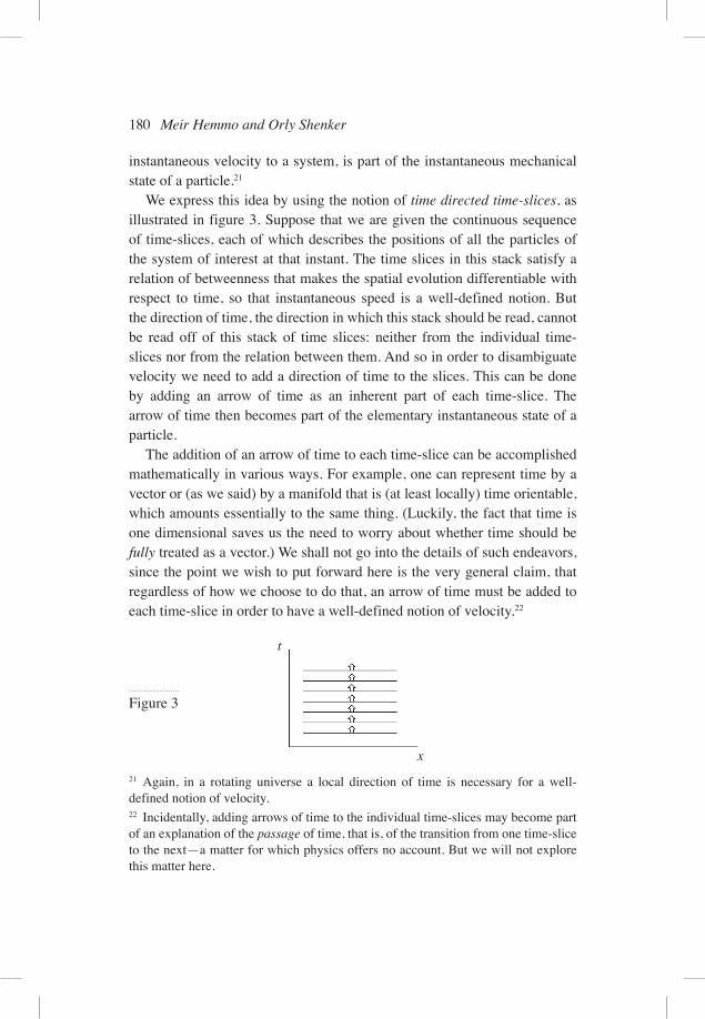
We express this idea by using the notion of time directed time-slices, as illustrated in figure 3. Suppose that we are given the continuous sequence of time-slices, each of which describes the positions of all the particles of the system of interest at that instant. The time slices in this stack satisfy a relation of betweenness that makes the spatial evolution differentiable with respect to time, so that instantaneous speed is a well-defined notion. But the direction of time, the direction in which this stack should be read, cannot be read off of this stack of time slices: neither from the individual time-slices nor from the relation between them. And so in order to disambiguate velocity we need to add a direction of time to the slices. This can be done by adding an arrow of time as an inherent part of each time-slice. The arrow of time then becomes part of the elementary instantaneous state of a particle.

The addition of an arrow of time to each time-slice can be accomplished mathematically in various ways. For example, one can represent time by a vector or (as we said) by a manifold that is (at least locally) time orientable, which amounts essentially to the same thing. (Luckily, the fact that time is one dimensional saves us the need to worry about whether time should be fully treated as a vector.) We shall not go into the details of such endeavors, since the point we wish to put forward here is the very general claim, that regardless of how we choose to do that, an arrow of time must be added to each time-slice in order to have a well-defined notion of velocity.22

21 Again, in a rotating universe a local direction of time is necessary for a well-defined notion of velocity. 22 Incidentally, adding arrows of time to the individual time-slices may become part of an explanation of the passage of time, that is, of the transition from one time-slice to the next—a matter for which physics offers no account. But we will not explore this matter here.

Figure 3

t

x


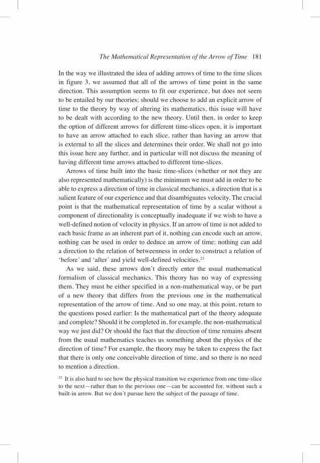
In the way we illustrated the idea of adding arrows of time to the time slices in figure 3, we assumed that all of the arrows of time point in the same direction. This assumption seems to fit our experience, but does not seem to be entailed by our theories; should we choose to add an explicit arrow of time to the theory by way of altering its mathematics, this issue will have to be dealt with according to the new theory. Until then, in order to keep the option of different arrows for different time-slices open, it is important to have an arrow attached to each slice, rather than having an arrow that is external to all the slices and determines their order. We shall not go into this issue here any further, and in particular will not discuss the meaning of having different time arrows attached to different time-slices.

Arrows of time built into the basic time-slices (whether or not they are also represented mathematically) is the minimum we must add in order to be able to express a direction of time in classical mechanics, a direction that is a salient feature of our experience and that disambiguates velocity. The crucial point is that the mathematical representation of time by a scalar without a component of directionality is conceptually inadequate if we wish to have a well-defined notion of velocity in physics. If an arrow of time is not added to each basic frame as an inherent part of it, nothing can encode such an arrow, nothing can be used in order to deduce an arrow of time; nothing can add a direction to the relation of betweenness in order to construct a relation of ‘before’ and ‘after’ and yield well-defined velocities.23

As we said, these arrows don’t directly enter the usual mathematical formalism of classical mechanics. This theory has no way of expressing them. They must be either specified in a non-mathematical way, or be part of a new theory that differs from the previous one in the mathematical representation of the arrow of time. And so one may, at this point, return to the questions posed earlier: Is the mathematical part of the theory adequate and complete? Should it be completed in, for example, the non-mathematical way we just did? Or should the fact that the direction of time remains absent from the usual mathematics teaches us something about the physics of the direction of time? For example, the theory may be taken to express the fact that there is only one conceivable direction of time, and so there is no need to mention a direction.23 It is also hard to see how the physical transition we experience from one time-slice to the next—rather than to the previous one—can be accounted for, without such a built-in arrow. But we don’t pursue here the subject of the passage of time.


One way of approaching these questions is by looking at other places where time appears in the equations of motion: in expression (3) the magnitude t appears in several places, and it may be instructive to compare the roles of its different appearances. This comparison, to which we now turn, will help us distinguish between the way the theory expresses the direction of processes in time, and the direction of time. On the way to distinguishing between the direction in time, and the direction of time, we will distinguish among three different concepts associated with reversing the magnitude t: velocity reversal, retrodiction, and time reversal. The distinction among these three concepts is important in order to understand the mathematical representation of the arrow of time in classical mechanics.

4. Velocity Reversal

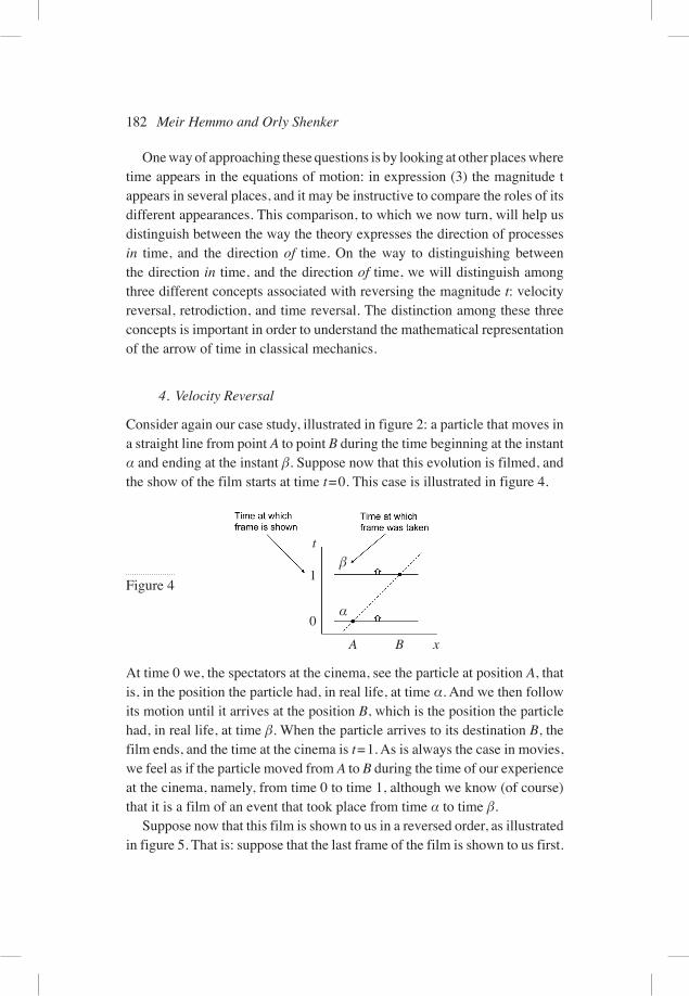
Consider again our case study, illustrated in figure 2: a particle that moves in a straight line from point A to point B during the time beginning at the instant α and ending at the instant β. Suppose now that this evolution is filmed, and the show of the film starts at time t=0. This case is illustrated in figure 4.

At time 0 we, the spectators at the cinema, see the particle at position A, that is, in the position the particle had, in real life, at time α. And we then follow its motion until it arrives at the position B, which is the position the particle had, in real life, at time β. When the particle arrives to its destination B, the film ends, and the time at the cinema is t=1. As is always the case in movies, we feel as if the particle moved from A to B during the time of our experience at the cinema, namely, from time 0 to time 1, although we know (of course) that it is a film of an event that took place from time α to time β.

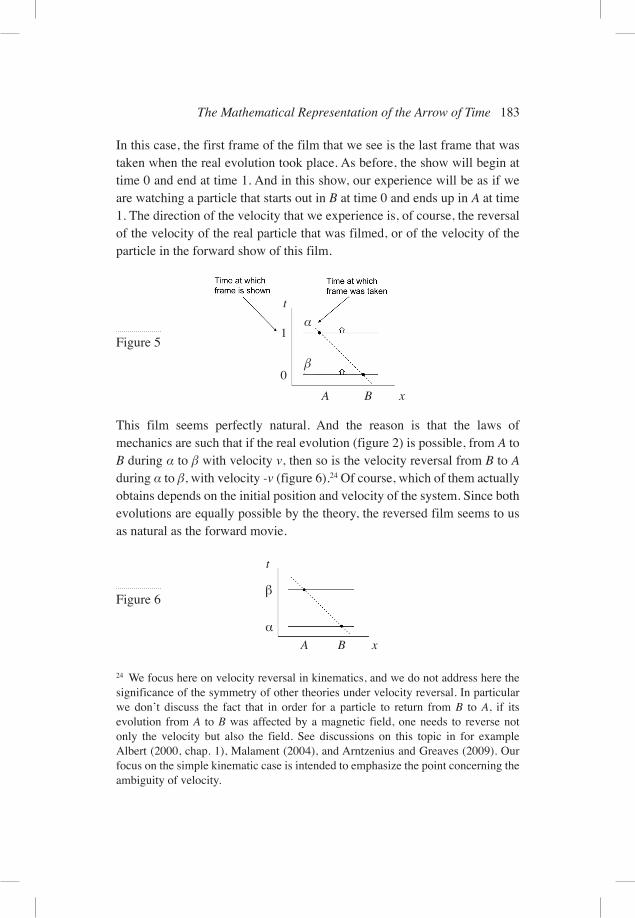
Suppose now that this film is shown to us in a reversed order, as illustrated in figure 5. That is: suppose that the last frame of the film is shown to us first.

Figure 41

β

α0

t

xBA


In this case, the first frame of the film that we see is the last frame that was taken when the real evolution took place. As before, the show will begin at time 0 and end at time 1. And in this show, our experience will be as if we are watching a particle that starts out in B at time 0 and ends up in A at time 1. The direction of the velocity that we experience is, of course, the reversal of the velocity of the real particle that was filmed, or of the velocity of the particle in the forward show of this film.

24 We focus here on velocity reversal in kinematics, and we do not address here the significance of the symmetry of other theories under velocity reversal. In particular we don’t discuss the fact that in order for a particle to return from B to A, if its evolution from A to B was affected by a magnetic field, one needs to reverse not only the velocity but also the field. See discussions on this topic in for example Albert (2000, chap. 1), Malament (2004), and Arntzenius and Greaves (2009). Our focus on the simple kinematic case is intended to emphasize the point concerning the ambiguity of velocity.

Figure 51

β

α

0

t

xBA

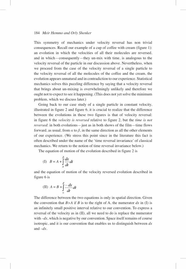
This film seems perfectly natural. And the reason is that the laws of mechanics are such that if the real evolution (figure 2) is possible, from A to B during α to β with velocity v, then so is the velocity reversal from B to A during α to β, with velocity -v (figure 6).24 Of course, which of them actually obtains depends on the initial position and velocity of the system. Since both evolutions are equally possible by the theory, the reversed film seems to us as natural as the forward movie.

Figure 6

α

β

t

xBA


This symmetry of mechanics under velocity reversal has non trivial consequences. Recall our example of a cup of coffee with cream (figure 1): an evolution in which the velocities of all their molecules are reversed, and in which—consequently—they un-mix with time, is analogous to the velocity reversal of the particle in our discussion above. Nevertheless, when we proceed from the case of the velocity reversal of a single particle to the velocity reversal of all the molecules of the coffee and the cream, the evolution appears unnatural and in contradiction to our experience. Statistical mechanics solves this puzzling difference by saying that a velocity reversal that brings about un-mixing is overwhelmingly unlikely and therefore we ought not to expect to see it happening. (This does not yet solve the minimum problem, which we discuss later.)

Going back to our case study of a single particle in constant velocity, illustrated in figure 2 and figure 6, it is crucial to realize that the difference between the evolutions in these two figures is that of velocity reversal: in figure 6 the velocity is reversed relative to figure 2, but the time is not reversed: in both evolutions—just as in both shows of the film—time flows forward, as usual, from α to β, in the same direction as all the other elements of our experience. (We stress this point since in the literature this fact is often described under the name of the ‘time reversal invariance’ of classical mechanics. We return to the notion of time reversal invariance below.)

The equation of motion of the evolution described in figure 2 is

(I) B = A +

and the equation of motion of the velocity reversed evolution described in figure 6 is

(II) A = B +

The difference between the two equations is only in spatial direction. Given the convention that B>A if B is to the right of A, the numerator dx in (I) is an infinitely small positive interval relative to our convention. To express a reversal of the velocity as in (II), all we need to do is replace the numerator with –dx, which is negative by our convention. Space itself remains of course isotropic, and it is our convention that enables us to distinguish between dx and –dx.


Equations (I) and (II) differ in the sign of the spatial direction of the evolution; let us turn to see the meaning of the way in which time is represented in these equations. Time appears in two places: in the denominator of the derivative, and in the integral. Let us see what these two appearances stand for.

5. Retrodiction

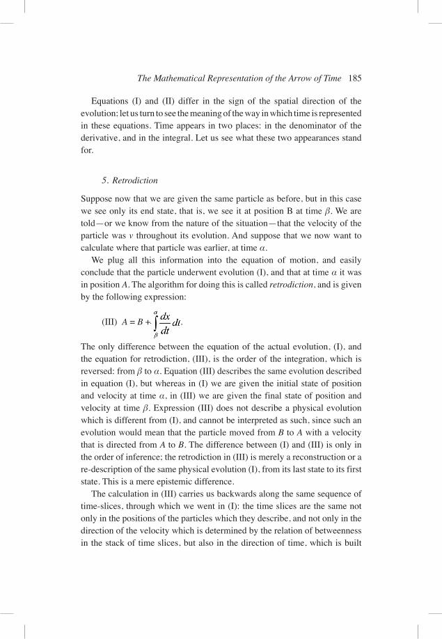
Suppose now that we are given the same particle as before, but in this case we see only its end state, that is, we see it at position B at time β. We are told—or we know from the nature of the situation—that the velocity of the particle was v throughout its evolution. And suppose that we now want to calculate where that particle was earlier, at time α.

We plug all this information into the equation of motion, and easily conclude that the particle underwent evolution (I), and that at time α it was in position A. The algorithm for doing this is called retrodiction, and is given by the following expression:

(III) A = B + .

The only difference between the equation of the actual evolution, (I), and the equation for retrodiction, (III), is the order of the integration, which is reversed: from β to α. Equation (III) describes the same evolution described in equation (I), but whereas in (I) we are given the initial state of position and velocity at time α, in (III) we are given the final state of position and velocity at time β. Expression (III) does not describe a physical evolution which is different from (I), and cannot be interpreted as such, since such an evolution would mean that the particle moved from B to A with a velocity that is directed from A to B. The difference between (I) and (III) is only in the order of inference; the retrodiction in (III) is merely a reconstruction or a re-description of the same physical evolution (I), from its last state to its first state. This is a mere epistemic difference.

The calculation in (III) carries us backwards along the same sequence of time-slices, through which we went in (I): the time slices are the same not only in the positions of the particles which they describe, and not only in the direction of the velocity which is determined by the relation of betweenness in the stack of time slices, but also in the direction of time, which is built


into each of the time slices: time goes forward in (III) as well as in (I). This means that the order of integration and the direction of time are independent of each other.

Finally, just to complete the picture, case (IV) is a retrodiction of evolution (II).

(IV) B = A + .

The relation between (IV) and (II) is the same as the relation between (III) and (I).

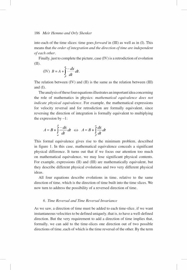
The analysis of these four equations illustrates an important idea concerning the role of mathematics in physics: mathematical equivalence does not indicate physical equivalence. For example, the mathematical expressions for velocity reversal and for retrodiction are formally equivalent, since reversing the direction of integration is formally equivalent to multiplying the expression by –1:

This formal equivalence gives rise to the minimum problem, described in figure 1. In this case, mathematical equivalence conceals a significant physical difference. It turns out that if we focus our attention too much on mathematical equivalence, we may lose significant physical contents. For example, expressions (II) and (III) are mathematically equivalent, but they describe different physical evolutions and two very different physical ideas.

All four equations describe evolutions in time, relative to the same direction of time, which is the direction of time built into the time slices. We now turn to address the possibility of a reversed direction of time.

6. Time Reversal and Time Reversal Invariance

As we saw, a direction of time must be added to each time-slice, if we want instantaneous velocities to be defined uniquely, that is, to have a well-defined direction. But the very requirement to add a direction of time implies that, formally, we can add to the time-slices one direction out of two possible directions of time, each of which is the time reversal of the other. By the term


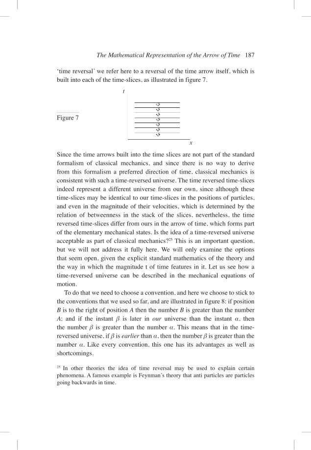
‘time reversal’ we refer here to a reversal of the time arrow itself, which is built into each of the time-slices, as illustrated in figure 7.

25 In other theories the idea of time reversal may be used to explain certain phenomena. A famous example is Feynman’s theory that anti particles are particles going backwards in time.

Since the time arrows built into the time slices are not part of the standard formalism of classical mechanics, and since there is no way to derive from this formalism a preferred direction of time, classical mechanics is consistent with such a time-reversed universe. The time reversed time-slices indeed represent a different universe from our own, since although these time-slices may be identical to our time-slices in the positions of particles, and even in the magnitude of their velocities, which is determined by the relation of betweenness in the stack of the slices, nevertheless, the time reversed time-slices differ from ours in the arrow of time, which forms part of the elementary mechanical states. Is the idea of a time-reversed universe acceptable as part of classical mechanics?25 This is an important question, but we will not address it fully here. We will only examine the options that seem open, given the explicit standard mathematics of the theory and the way in which the magnitude t of time features in it. Let us see how a time-reversed universe can be described in the mechanical equations of motion.

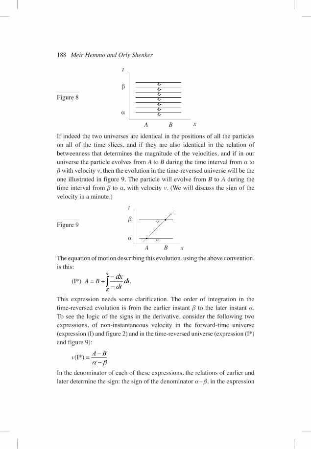
To do that we need to choose a convention, and here we choose to stick to the conventions that we used so far, and are illustrated in figure 8: if position B is to the right of position A then the number B is greater than the number A; and if the instant β is later in our universe than the instant α, then the number β is greater than the number α. This means that in the time-reversed universe, if β is earlier than α, then the number β is greater than the number α. Like every convention, this one has its advantages as well as shortcomings.

Figure 7

t

x


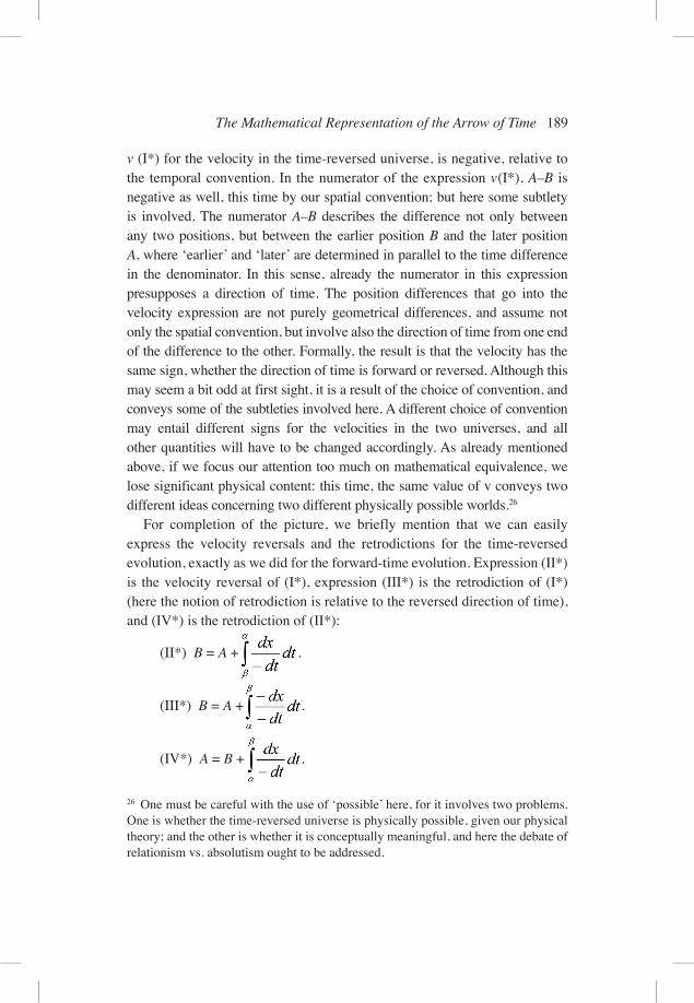
If indeed the two universes are identical in the positions of all the particles on all of the time slices, and if they are also identical in the relation of betweenness that determines the magnitude of the velocities, and if in our universe the particle evolves from A to B during the time interval from α to β with velocity v, then the evolution in the time-reversed universe will be the one illustrated in figure 9. The particle will evolve from B to A during the time interval from β to α, with velocity v. (We will discuss the sign of the velocity in a minute.)

Figure 8

α

β

t

xBA

Figure 9

α

β

t

xBA

The equation of motion describing this evolution, using the above convention, is this:

(I*) A = B + .

This expression needs some clarification. The order of integration in the time-reversed evolution is from the earlier instant β to the later instant α. To see the logic of the signs in the derivative, consider the following two expressions, of non-instantaneous velocity in the forward-time universe (expression (I) and figure 2) and in the time-reversed universe (expression (I*) and figure 9):

v(I*) =

In the denominator of each of these expressions, the relations of earlier and later determine the sign: the sign of the denominator α – β, in the expression


v (I*) for the velocity in the time-reversed universe, is negative, relative to the temporal convention. In the numerator of the expression v(I*), A–B is negative as well, this time by our spatial convention; but here some subtlety is involved. The numerator A–B describes the difference not only between any two positions, but between the earlier position B and the later position A, where ‘earlier’ and ‘later’ are determined in parallel to the time difference in the denominator. In this sense, already the numerator in this expression presupposes a direction of time. The position differences that go into the velocity expression are not purely geometrical differences, and assume not only the spatial convention, but involve also the direction of time from one end of the difference to the other. Formally, the result is that the velocity has the same sign, whether the direction of time is forward or reversed. Although this may seem a bit odd at first sight, it is a result of the choice of convention, and conveys some of the subtleties involved here. A different choice of convention may entail different signs for the velocities in the two universes, and all other quantities will have to be changed accordingly. As already mentioned above, if we focus our attention too much on mathematical equivalence, we lose significant physical content: this time, the same value of v conveys two different ideas concerning two different physically possible worlds.26

For completion of the picture, we briefly mention that we can easily express the velocity reversals and the retrodictions for the time-reversed evolution, exactly as we did for the forward-time evolution. Expression (II*) is the velocity reversal of (I*), expression (III*) is the retrodiction of (I*) (here the notion of retrodiction is relative to the reversed direction of time), and (IV*) is the retrodiction of (II*):

(II*) B = A + .

(III*) B = A + .

(IV*) A = B + .

26 One must be careful with the use of ‘possible’ here, for it involves two problems. One is whether the time-reversed universe is physically possible, given our physical theory; and the other is whether it is conceptually meaningful, and here the debate of relationism vs. absolutism ought to be addressed.


There is no need to enter into the details of these equations—they repeat what we said about the forward-time kinematics, replacing the order of time wherever necessary.

Classical mechanics happens to be such that formally, all its fundamental27 laws hold in this imaginary time-reversed universe: the general form of the laws of nature is exactly the same in both universes. As a result, by looking at the fundamental laws of nature one is unable to tell whether one inhabits this universe or the other. In this sense, classical mechanics is time reversal invariant. Whether or not the fact that the two universes are empirically indiscernible in this sense makes the very notion of time reversal meaningless is an old debate, that goes back at least to the exchanges of Newton, Leibniz, and Clarke.28

7. Conclusion

Be the physical significance of the time-reversed universe as it may, the very idea that our time does have a direction is an assumption we have to make, in order to obtain a non ambiguous notion of velocity. And once we have this direction, we can break the symmetry between past and future in our fundamental theories, concerning our universe. Recall that we started out this discussion by describing the minimum problem, that is, the well-known result that the retrodictions of our fundamental theories are such that it is highly likely that the past was not as we remember it, but rather was similar to the predicted future. We said that the only available solution of this problem, by way of the Past Hypothesis, says that as a matter of fact the universe was as we remember it, despite the contrary probabilistic claims. But to make sense of this hypothesis, as part of our physics, we need a difference between past and future, within the fundamental theories. And we saw in this paper that, in fact, the very notion of a well-defined velocity already assumes such a difference. Although the standard mathematical representation of time in classical mechanics does not express a direction

27 The term ‘fundamental’ is meant to exclude the theory of thermodynamics, which describes the effective appearance at the macroscopic level. If the fundamental theories are true of the world (to some extent and in some sense), then they should be able to explain this effective appearance. For a discussion of the difficulties in coming up with a proof of such entailment see Hemmo and Shenker (2012).28 See Alexander (1955).


of time, the elementary notion of a well-defined velocity already assumes such a direction. We can either change the mathematics to express this fact, or, if we want to keep the mathematics unchanged, the way to represent this direction of time is by adding an arrow of time to the elementary time-slices, that is, to the definition on an elementary mechanical state of a particle. Once we realize that the most elementary physics, at the level of the description of an instantaneous state of a single particle, already assumes an arrow of time, we at least have a way to express the Past Hypothesis. Whether or not it also makes the Past Hypothesis a reasonable or acceptable solution to the minimum problem is another matter.29

Department of Philosophy, University of Haifa. [email protected]

Program in the History and Philosophy of Science, The Hebrew University of Jerusalem. [email protected]

BibliographyAlbert, David. 2000. Time and Chance. Harvard University Press.Alexander H. 1955. The Leibniz-Clarke Correspondence. Manchester University

Press.Arntzenius, Frank. 2000. “Are There Really Instantaneous Velocities?” Monist 83:

187–209.Arntzenius, Frank and Hilary Greaves. 2009. “Time Reversal in Classical Electro-

magnetism,” British Journal for the Philosophy of Science 60 (3): 557–584.Augustine. Confessions. Translated and edited by Albert C. Outler. New edition. New

York: Dover, 2002.Earman, John. 1986. A Primer on Determinism. Dordrecht: Kluwer.Feynman, Richard. 1965. The Character of Physical Law. MIT Press.Hemmo, Meir and Orly Shenker. 2006. “Von Neumann’s Entropy Does Not

Correspond to Thermodynamic Entropy,” Philosophy of Science 73:153–174.Hemmo, Meir and Orly Shenker. 2012. The Road to Maxwell’s Demon. Cambridge

University Press. Forthcoming.Malament, David. 2004. “On the Time Reversal Invariance of Classical Electro-

magnetic Theory,” Studies in History and Philosophy of Modern Physics 35B (2): 295–315.

29 See Hemmo and Shenker (2012, chap. 10).


Newton, Isaac. 1687. The Mathematical Principles of the Philosophy of Nature. English translation by Andrew Mott, 1729. Berkeley: University of California Press, 1962.

Putnam, Hilary. 1967. “Time and Physical Geometry,” Journal of Philosophy 64 (8): 240–247.

Reichenbach, Hans. 1956. The Direction of Time. University of California Press.Steiner, Mark. 1998. The Applicability of Mathematics as a Philosophical Problem.

Harvard University Press.Von Neumann, John. 1932. The Mathematical Foundations of Quantum Mechanics.

Translated by Robert T. Beyer. Princeton: Princeton University Press, 1955. Wigner, Eugene. 1960. “The Unreasonable Effectiveness of Mathematics in the

Natural Sciences,” Communications in Pure and Applied Mathematics, 13 (I). Reprinted in E. Wigner, Symmetries and Reflections, 222–237. Bloomington: Indiana University Press, 1967.

The Mathematical Representation of the Arrow of Time (2012)

Documents

Transcript of The Mathematical Representation of the Arrow of Time (2012)