- 0 -

1 2 biblio.ugent.be 3 4 The UGent Institutional Repository is the electronic archiving and dissemination platform for 5 all UGent research publications. Ghent University has implemented a mandate stipulating that 6 all academic publications of UGent researchers should be deposited and archived in this 7 repository. Except for items where current copyright restrictions apply, these papers are 8 available in Open Access. 9 This item is the archived peer-reviewed author-version of: 10 11 Title: The kinetic plot method applied to gradient chromatography: theoretical 12 framework and experimental validation. 13 14 Authors: K. Broeckhoven, D. Cabooter, F. Lynen, P. Sandra and G. Desmet 15

In: 16 17 JOURNAL OF CHROMATOGRAPHY A Volume: 1217 Issue: 17 Pages: 2787-2795 18 Published: APR 23 2010 19 20 Optional: 21 http://www.sciencedirect.com/science?_ob=MImg&_imagekey=B6TG8-4YF5R6F-6-22 D&_cdi=5248&_user=794998&_pii=S0021967310002281&_orig=search&_coverDate=0423 %2F23%2F2010&_sk=987829982&view=c&wchp=dGLbVzb-24 zSkWA&md5=49389f0bcb9b465bd96117f23c9709bb&ie=/sdarticle.pdf 25 26 To refer to or to cite this work, please use the citation to the published version: 27 28 K. Broeckhoven, D. Cabooter, F. Lynen, P. Sandra, G. Desmet; J. Chromatogr. A 1217(17), 29 2787-2795. 30 31 doi:10.1016/j.chroma.2010.02.023 32 33 34

35 36

37

38

39

40

41

42

- 1 -

1

The kinetic plot method applied to gradient chromatography: theoretical 2

framework and experimental validation 3

4

K. Broeckhoven1, D. Cabooter1, F. Lynen2, P. Sandra2 and G. Desmet1,* 5

6

7

(1) Vrije Universiteit Brussel, Department of Chemical Engineering, Pleinlaan 2, 1050 Brussels, Belgium 8

(2) Dept. of Organic Chemistry, Universiteit Gent, Krijgslaan 281 S4-Bis, 9000 Gent, Belgium 9

* Corresponding author. Pleinlaan 2, 1050 Brussels, Belgium. 10

Phone: (+)32.(0)2.629.32.51. Fax: (+)32.(0)2.629.32.48. E-mail: gedesmet@vub.ac.be 11

12

- 2 -

Keywords: kinetic performance, gradient elution, band broadening, peak compression, numerical 1

simulation 2

3

Abstract 4

The kinetic plot method, originally developed for isocratic separations, was extended to the practically 5

much more relevant case of gradient elution separations. A set of explicit as well as implicit data 6

transformation expressions has been established. These expressions can readily be implemented in any 7

calculation spread-sheet program, and allow to directly turn any experimental data set representing the 8

relation between the separation efficiency and the flow rate measured on a single column into the kinetic 9

performance limit curve of the tested separation medium. Since the kinetic performance limit curve is 10

based on an extrapolation to columns with a different length, it should be realized that the curve is only 11

valid under the assumption that the gradient time and the delay time (if any) are adapted such that the 12

analytes are subjected to the same relative mobile phase history when the column length is changed. 13

14

Both experimental and numerical data are presented to corroborate the fact that the kinetic performance 15

limit curves that are obtained using the proposed expressions are indeed independent of the column 16

length the experimental data were collected in. Deviations might arise if excessive viscous heating 17

occurs in columns with a pronounced non-adiabatic thermal behaviour. 18

19

1. Introduction 20

In the pursuit of ever faster or more efficient LC separations, HPLC systems with smaller particles, higher 21

pressures and higher temperatures are currently being developed and commercialized [1-7]. And with 22

the advent of monolithic columns and porous shell particles, also different support formats are being 23

considered [8-10]. To guide this research and the decision analysts have to make when considering the 24

purchase of new systems, a uniform comparison method is needed. 25

26

The classical Van Deemter plot does not allow to directly show which approach yields the highest 27

separation resolution in a given time, or which approach yields a given resolution in the shortest possible 28

time (for the general performance of a chromatographic system is also determined by its pressure-drop 29

characteristics). A plot of efficiency or resolution versus the time calculated for the largest available 30

pressure on the other hand directly shows which system would perform best in a given range of required 31

efficiency, resolution or analysis time. Referring to this type of plot with the general name of "kinetic 32

plots", it should be reminded that the use of plots of separation quality versus time already dates back 33

from the classical work of Giddings in 1965 [11]. Knox [12] and Guiochon [13] used the kinetic plot 34

- 3 -

approach to compare the performance of packed bed columns with open-tubular columns in the 1

seventies and early eighties. In 1997, Hans Poppe proposed to plot t0/N versus N instead of t0 versus N 2

to obtain a clearer view on the C-term contribution [14]. 3

4

Common to the approach adopted by these and other authors [10,15] is that they used a computer 5

optimization or numerical search to find the kinetic optimum. The novelty of the approach presented by 6

our group in 2005 [16] therefore was not a retransformation of the axes (t versus N or t/N2 versus N 7

instead of t/N versus N), but the presentation of two simple mathematical expressions that allow to turn 8

any experimental data set of H versus u-data (or N versus F-data) directly into a kinetic plot, without the 9

need for a numerical optimization algorithm. The availability of these two simple data transformation 10

expressions (cf. Eqs.(6-7) in Desmet et al. [16]), providing a new and more straightforward way to 11

produce kinetic plots, opened the way to a broad use of kinetic plot comparisons [17,18]. 12

13

The theory underlying this so-called kinetic plot method (KPM) was however limited to isocratic 14

separations, whereas the majority of the separations is run under gradient elution conditions. Kinetic 15

plots under gradient conditions have recently been presented by Wang et al. and Zhang et al. [10,15], 16

but these plots were still obtained using a computerized constrained optimization algorithm (implemented 17

via a Solver add-in of MS Excel). Mathematical expressions that can directly transform any experimental 18

set of gradient efficiency or peak capacity versus flow rate data directly into a kinetic plot curve are still 19

lacking. The present study therefore aims at providing a theoretical framework to extend the KPM to 20

gradient elution conditions. What results is a broader framework, covering both the isocratic and gradient 21

case, and yielding a set of explicit and implicit data transformation expressions. 22

23

2. Separation efficiency measures 24

Regardless of whether the elution is isocratic or gradient, the efficiency of a chromatographic system can 25

be characterized by a column plate height H or plate count N, which are fundamentally defined [11] with 26

respect to the spatial variance of the bands in the column: 27

N

L

LH

2

x =σ= (1) 28

Band widths are however usually measured in time and not in space. In that case, the information about 29

H needs to be retrieved from the temporal variance σt2 of the peak observed at the detector. The value 30

of this variance is usually directly calculated by the instrument software, and is linked to H and N via: 31

0

elut

0

elutelut

0t

u

)k1(HL

u

)k1(HN)k1(

N

t +⋅⋅=+⋅⋅=+⋅=σ (2) 32

- 4 -

A key parameter in Eq. (2) is the retention factor (kelut) experienced by the analytes at the moment of 1

elution. Under isocratic conditions, this retention factor is equal to the observed or effective retention 2

factor k (defined as k=(tR-t0)/t0) [19-21], so that Eq. (2) can be straightforwardly used to calculate H and 3

N. Under gradient conditions, however, kelut is always smaller than the effective k and can also not be 4

directly measured. In that case, one either needs to determine kelut using the Linear Solvent Strength-5

model (LSS-model, see Eq. (28)) or any of the more complex mathematical non-LSS models such as 6

those described in [22]. Alternatively, one can first determine the mobile phase composition at which the 7

component elutes and then perform an isocratic elution experiment at this composition to measure kelut. 8

Both approaches anyhow require additional experiments and constitute a potential source of additional 9

measurement errors. 10

11

Given this and other complexities, plate heights are seldom used in gradient elution (see the Supporting 12

Material, SM, Part 1.1 for a broader discussion of the problems related to the use of the plate height 13

concept under gradient elution elution). Instead, it is often preferred to directly use the observed σt or the 14

resulting peak capacity, np, as both measures are true "what you see is what you get"-variables. 15

16

The peak capacity of a column is most generally expressed in an integral form [23,24]: 17

∫ σ⋅+=

R

0

t

t t

p dt4

11n (3) 18

Eq. (3) can however only be used if the variation of σt with the time is exactly known. If this is not the 19

case, the integral can be split up in parts, assuming that the peak width of each eluting band is represen-20

tative for the range of elution between its own moment of elution and that of the preceding peak [25]: 21

∑= +

+

σ⋅−

+=n

1i 1i,t

i,R1i,R

p4

tt1n (4) 22

An even more simplified peak capacity definition is based on the average band width (wp,av=4⋅σt,av) [23]: 23

∑=

σ⋅=σn

1i

i,tav,tn

1 (5) 24

av,t

1n,R

p4

tt1n

σ⋅−

+= (6) 25

Both Eq. (4) and (6) relate to a sample-based peak capacity. Sometimes (as in the present study), the t0-26

marker is included as component number i=1, in which case the elution window in Eqs. (4) and (6) 27

extends between t0 and tR,n (wherein n is the number of sample components +1). In other cases, the 28

peak capacity is calculated based on the gradient time tG. Yet other peak capacity definitions exist in 29

- 5 -

literature [15,24,26-28]. All existing np-definitions however display the same square-root length-1

dependency (as shown in the SM, section 2.3), expressed by Eq. (18) further on, so that, for what 2

concerns the application of the KPM, they all behave the same. 3

4

In the present work, the definition used in Eq. (4) (with i=1 representing the t0 marker) has been used 5

throughout all presented figures and data sets. For the sake of clarity, it should also be remarked that the 6

effective retention factor k used in the present study is purely based on the observed peak retention 7

times (k=(tR-t0)/t0), for isocratic as well as for gradient elution (the effective k is in the literature on 8

gradient separations k sometimes also denoted as kg [23]). It should therefore also be noted that k no 9

longer equals the product of the equilibrium constant and the phase ratio in the column in the gradient 10

case. 11

12

3. General kinetic plot theory valid for both isocratic and gradient elution 13

14

3.1 General concept 15

The kinetic performance of a chromatographic system can be defined as the efficiency N or peak 16

capacity np it can generate in a certain time. This also depends on the permeability of the system, so that 17

the kinetic performance is determined by the three following basic expressions [11,12]: 18

0

0u

Lt = (7) 19

H

LN = (8) 20

v

0

K

LuP

⋅η⋅=∆ (9) 21

If desired, the efficiency N can be replaced by the peak capacity np. In this case, the relation between np 22

and σt (see e.g., Eq. (4)) and that between σt and L (see Eq. (2)) need to be combined into an 23

expression describing np as a function of L, and this expression should then replace Eq. (8). This is of 24

course more complicated but nevertheless still leads to a mathematical expression that is straight-25

forwardly applicable. It might also be preferred to replace the t0-time by the total time tR (via tR=t0⋅(1+k)) 26

or to replace N by the effective plate number Neff (via Neff=N⋅k2/(1+k)2 [16,29]), but these modifications 27

also do not change anything fundamental to the optimization procedure below. 28

29

Defining now the kinetic performance limit (KPL) of a given chromatographic support as the set of 30

optimal column lengths and flow rates wherein the complete set of possible N- or np- values is achieved 31

- 6 -

in the shortest possible time, or, equivalently, wherein a maximal N or np is achieved over the complete 1

range of possible analysis times, it can be shown (see SM, Part 2.1) that both conditions are simulta-2

neously met if the column pressure-drop is equal to the maximally possible or allowable pressure ∆Pmax:3

kinetic performance limit is achieved ⇔ ∆P=∆Pmax (10) 4

5

Putting ∆P=∆Pmax in Eq. (9) and solving the set of equations given by Eqs. (7-9) hence suffices to 6

calculate the KPL of a given chromatographic support (note that this KPL is only valid for the considered 7

mobile phase and sample, see Section 3.4). Solving Eqs. (7-9) can be done in a purely algebraic manner 8

and leads to the set of explicit kinetic plot expressions shown in the 3rd column of Table 1 (derivation: 9

see Part 2.2 of the SM). These expressions transform the efficiency (or np or Rs) measured in a column 10

with length L and given flow rate F (and corresponding pressure-drop ∆P) into the efficiency (or np or Rs) 11

one would obtain when applying the same velocity or flow rate in a column with a length selected such 12

that ∆P=∆Pmax. 13

14

Whereas a Van Deemter curve only contains part of the kinetic information (it lacks the pressure-drop 15

information), the so-called kinetic plot or kinetic performance limit (KPL)-curve directly represents the 16

complete series of optimal kinetic performances (one data point for each possible flow rate) one can 17

expect from a given support under the employed mobile phase conditions. The KPL-curve is therefore 18

ideally suited as a universal performance measure, for example allowing to directly compare monolithic 19

columns with fully and superficially porous particles, in a direct "what you see is what you get" plot. 20

21

3.2 Assumptions underlying the validity of the kinetic performance limit curve 22

Any established KPL-curve in fact corresponds to a prediction of the optimal kinetic performances that 23

can be expected in an imaginary set of different columns, all with different length but filled with the same 24

support and operated at ∆P=∆Pmax. This prediction is based on a set of efficiency measurements 25

conducted on a single column with fixed length. It hence needs to be ascertained that this length extra-26

polation is allowed and that the position of the KPL-curve in the (efficiency, time)-plane is independent of 27

the length of the column that was used to collect the experimental data upon which it is based. 28

29

The main assumption underlying the simultaneous solution of Eqs. (7-9) is that the parameters that are 30

contained in it are mutually independent. This implies that any data transformation based on Eqs. (7-9) is 31

also based on the assumption that H and η are independent of the column length. When calculating a 32

KPL-curve involving information about the retention times (which is e.g., the case when plotting the tR-33

- 7 -

time versus the sample based peak capacity), the effective retention factors (k) of the individual sample 1

components should be independent of the column length as well. 2

3

Hence, one can conclude from the above that a physically valid KPL-curve can only be obtained under 4

conditions wherein the effective H, η and k are length-independent. If satisfied, the validity then holds 5

regardless whether an isocratic or gradient elution is being considered, since it was not needed to 6

distinguish between both elution modes in any of the above. 7

8

In the absence of high-pressure operation effects, and provided the flow rate, the sample and the mobile 9

phase composition remain the same, the assumption of a length-independent plate height and elution 10

pattern is commonly accepted under isocratic conditions (see SM, part 2.3 for the exceptions to this con-11

dition). Under gradient conditions, it can be shown [19,22,23,30,31] (see SM, part 1.1.3 and 2.3) that the 12

necessary and sufficient condition of a length-independent plate height and elution window is that the 13

analytes are subjected to the same "relative mobile phase history". The latter term (in short "φ-history") 14

denotes the series of φ-values experienced by the analytes at each given dimensionless position x' 15

(x'=x/L) in the column. The condition of an identical relative φ-history also automatically guarantees that 16

the analytes experience an identical η-history (see discussion of Eq. (S-61) in SM) 17

18

It can be shown (see SM part 1.1.2) for the case of a linear gradient that analytes will always experience 19

the same relative mobile phase history provided the gradient steepness β⋅t0, the initial mobile phase φ0 20

composition and the ratio and tdelay/t0 (if any tdelay is present) are kept the same, regardless of the column 21

length or the applied flow rate. The time based gradient steepness β used in this statement is usually 22

defined as: 23

Gstartend

0t

tttend

φ∆=−

φ−φ=β (11) 24

whereas the delay time tdelay is defined as the time elapsing between the injection and the instant at 25

which the gradient profile reaches the front of the column (note that in the general case tdelay is equal to 26

the system dwell time (tdwell) + any additional delay time introduced in the gradient program). 27

28

Based on expressions found in literature [19,22,32], it can also be shown that, when the analytes 29

experience the same relative φ-history, also the peak compression factor G can be expected to be 30

independent of the column length (see SM part 1.1.3). 31

32

- 8 -

As a result, it can be concluded that the length extrapolation underlying the establishment of a KPL-curve 1

is only valid under the strict assumption that each original data point and its corresponding extrapolated 2

data point are obtained under the same φ-history. For gradient elutions, this implies that, since a change 3

in length inevitably involves a change in t0 (flow rate is fixed during the KPL transformation), the 4

extrapolation is only correct when tG is adapted to keep the same β⋅t0 (or equivalently, tG/t0 constant). If 5

the gradient program contains a delay time tdelay (e.g., because the system has a significant dwell 6

volume, i.e. volume between pump and injector), the gradient programming also has to be adjusted so 7

that the ratio tdelay/t0 is kept constant, as discussed in more detail in the SM (Part 1.1.2). Alternatively, a 8

delayed injection can be used to eliminate the effect of the system dwell volume (see SM, Part 2.3 for 9

more details). 10

11

When ultra-high-pressure effects come into play, just keeping the same φ-history is no longer sufficient 12

to ensure length-independent H-, η- and k-values (in both the isocratic and gradient mode). This is 13

discussed in more detail in the SM part 2.3, where a simple correction formula that compensates for 14

most of the error is given (Eq. S-62). 15

16

3.3 Physical interpretation of the KPM and implicit KPM-expressions 17

Since the data transformation underlying the KPM transforms the experimental data by keeping each 18

measured efficiency data point together with its corresponding u0-value, the u0-velocity (or equivalently 19

the flow rate F) is in fact treated as a fixed variable. This leaves the column length as the only remaining 20

freely changeable variable that can be used to ensure that ∆P=∆Pmax. As can be noted by rewriting Eq. 21

(9) and making the traditional assumption (see also SM, Part 2.3) that Kv and η are constants, this leads 22

to: 23

η⋅∆⋅=

0

v

u

PKL and

η⋅∆⋅=0

maxvmax

u

PKL (12) 24

Hence, when calculating the kinetic performance limit while keeping u0-constant, the condition of 25

achieving the maximal pressure simply corresponds to maximizing the column length (SM, Part 2.2): 26

∆P = ∆Pmax at constant u0 ⇔ L = Lmax (13) 27

28

As a consequence, it suffices to replace L by Lmax in the expressions for N and np to transform a set of 29

experimental column performance measurements into the corresponding KPL-curve. This is fully 30

elaborated in the SM (Part 2.2). Table 1 summarizes the results obtained there, and provides all possible 31

conversion expressions between the performance characteristics measured on a given column with fixed 32

- 9 -

length and the corresponding KPL-curve. As indicated, this transformation can occur using either the 1

explicit (3rd column) or implicit (4th column) dependence on H. 2

3

A drawback of the explicit equations when used in gradient elution is that they require the calculation of a 4

gradient plate height. Although this is perfectly possible (illustrated in the SM, Part 1.2), it strongly 5

complicates things. The beauty of the implicit expressions is that they circumvent this problem, as they 6

are directly based on the physical meaning of the KPM and hence only require the calculation of a so-7

called column length rescaling factor λ: 8

exp

max

P

P

∆∆=λ (14) 9

which is a readily obtainable experimental parameter (∆Pexp is the maximum column pressure drop 10

experienced during the gradient run conducted to measure a given Nexp or np,exp and t0,exp-data point, i.e. 11

the value obtained by subtracting the extra column pressure drop). Using this λ-value, the implicit kinetic 12

plot expressions allow to directly calculate the corresponding KPL-variables (subscript "KPL") from the 13

experimentally measured column performance measures (subscript "exp") on a single column, via: 14

15

exp,0KPL,0 tt ⋅λ= (15) 16

exp,RKPL,R tt ⋅λ= (16) 17

expKPL NN ⋅λ= (17) 18

)1n(1n ,exppKPL,p −⋅λ+= (18) 19

exp,tKPL,t σ⋅λ=σ (19) 20

expi,s,KPLi,s, RR ⋅λ= (20) 21

expKPL LL ⋅λ= (21) 22

23

Since every experimental data point is obtained for a different ∆Pexp, it is needless to say that λ is 24

different for each measured data point, in agreement with Eq. (22) given here below. Working under 25

conditions wherein the structural and physicochemical column parameters can be considered to be 26

pressure-independent (see SM, part 2.3), it can be readily derived from Eqs. (14) and (12) that λ is 27

inversely proportional to the mobile phase velocity u0 or flow rate F: 28

0

1

u

cst=λ or F

cst2=λ (22) 29

- 10 -

3.4 Comparing different stationary phase types using the KPM 1

In Section 3.2, it was noted that the KPM only leads to a correct rescaling from one column length to the 2

other provided that the analytes are subjected to the same relative φ-history. Considering only one type 3

of particles (or stationary phase), this corresponds to keeping the value of β⋅t0, tdelay/t0 and φ0 constant. 4

However, when comparing different stationary phases (which generally each have a different retention 5

behaviour), the condition of an identical relative φ-history no longer suffices to keep the same elution 6

window. 7

8

In our opinion, the best way out of this is that the comparison of different stationary phases should occur 9

by first selecting a sample of interest, and then vary φ0, φend and β⋅t0 for each phase independently until 10

the best KPL-curve (or set of intersecting best curves) for that specific stationary phase is obtained. Per-11

forming this optimization for each stationary phase independently, one can then compare the different 12

stationary phases, each for their own individually optimized optimum, i.e., the KPL-curve (or set of 13

intersecting curves) lying the far most to the bottom and to the right of the time versus peak capacity plot. 14

15

In a variant to this, and assuming that the LSS-model would apply, a comparison between different 16

phases can be achieved by keeping the same φ0 and adapting β such that the same value of Sav⋅β⋅t0 is 17

obtained (with Sav the sample-averaged solvent strength parameter). This technique was illustrated by 18

Zhang et al. [10] and allows to compare different phases in a more or less similar elution window. 19

20

4. Experimental and computational procedures 21

4.1 Experimental 22

Uracil, benzene, naphthalene, phenanthrene, methyl-, ethyl-, propyl and butylparaben were purchased 23

from Sigma-Aldrich (Steinheim, Germany). Acetonitrile (ACN), methanol (MeOH) and water (all HPLC 24

grade) were also purchased from Sigma-Aldrich. HALO Fused Core C18 columns (150 x 2.1 mm, 2.7 25

µm) were purchased from Advanced Materials Technologies (Wilmington, DE, USA). Zorbax Stable 26

Bond C18 columns (50mm×4.6 mm, 1.8 µm; 150mm×4.6 mm, 3.5 µm and 150mm×4.6 mm, 5 µm) were 27

purchased from Agilent Technologies (Diegem, Belgium). 28

29

For the HALO columns, all experiments were conducted in the gradient mode with an acetonitrile/water 30

mobile phase. The initial mobile phase composition was 50%/50% (v/v) acetonitrile/water and the 31

gradient steepness (β⋅t0) was kept constant during the measurement of the gradient van Deemter curves 32

(different gradient steepness values were obtained by putting β⋅t0 equal to 0.008, 0.016, 0.024, 0.048 33

- 11 -

and 0.064). The initial value of φ and the range over which it was varied, was thus the same in each 1

experiment, which implies that only the gradient time tG was changed to maintain constant ratio of tG/t0 2

(or equivalently β⋅t0) for the different gradient steepness’s. Chromatograms were recorded for at least 3

nine different velocities on 1 column, for at least 5 velocities on the 2 coupled columns and for 3 4

velocities on the 4 coupled columns. The columns were tested on an Agilent 1200 HPLC system (Agilent 5

Technologies, Waldbronn, Germany) with a diode array detector with a 1.7 µL detector cell and a binary 6

pump. The system was operated with Agilent Chemstation software. Samples consisting of 0.02 mg/mL 7

uracil, 0.1 mg/mL benzene, 0.05 mg/mL naphthalene and 0.05 mg/mL phenanthrene were dissolved in 8

the initial mobile phase. The injected sample mixture volume was 1 µL. Absorbance values were 9

measured at 210 nm with a sample rate of 80 Hz. 10

11

For the Zorbax columns, all experiments were conducted in the gradient mode with a methanol/water 12

mobile phase. The initial mobile phase composition was 45%/55% (v/v) methanol/water and the gradient 13

steepness (β⋅t0) was kept constant during the measurement of the gradient van Deemter curves (β⋅t0 14

equal to 0.020) for the different particle sizes. The columns were tested on a Dionex Ultimate 3000 15

system (Dionex Benelux, Amsterdam, The Netherlands) with a diode array detector with a 2.5 µL 16

detector cell and a binary pump. The system was operated with the Dionex Chromeleon software 17

(Dionex, Munchen, Germany). Samples consisting of 0.02 mg/mL uracil, 0.02 mg/mL methylparaben, 18

0.02 mg/mL ethylparaben, 0.04 mg/mL propylparaben, and 0.04 mg/mL butylparaben were dissolved in 19

the initial mobile phase. The injected sample mixture volume was 2 µL. Absorbance values were 20

measured at 254 nm with a sample rate of 50 Hz. 21

22

The system dwell volumes were determined using the procedure described in [33] and were determined 23

as 450 µl for the Agilent 1200 system and 610 µl for the Dionex Ultimate 3000 system. 24

25

For every component in the chromatogram, the variances were calculated using the peak width at half 26

height. All experiments were conducted at a temperature of 30°C. The efficiency measurements were 27

conducted from the lowest flow rate (0.05 mL/min) up to the maximal available pressure of the 28

instrument (600 bar) for the HALO columns. The Zorbax columns were tested from the lowest flow rate 29

(0.062 ml/min) up to the maximal pressure allowed by the column hardware (400 bar for the 3.5 en 5µm 30

particles and 600 bar for the 1.8µm particle column). 31

32

- 12 -

All reported data were obtained after correction for the system band broadening (σ²ec), t0-time (tec) and 1

pressure drop (∆Pec), measured by removing the column from the system and replacing it with a zero 2

dead volume connection piece [7]: 3

ec2

total2

col2 σ−σ=σ (23) 4

ectotal,0col,0 ttt −= (24) 5

ectotal,Rcol,R ttt −= (25) 6

ectotalcol PPP ∆−∆=∆ (26) 7

The extra column band broadening was measured for each component separately, using a mobile phase 8

composition that resulted isocratically in the same k values as during the gradient run. The contribution 9

of the system to the total band variance was on the HALO columns always less than 5% for 10

phenanthrene and even smaller on the Zorbax columns. Eq. (23) however overestimates the contribution 11

of the extra column band broadening in gradient elution, since it lumps both the pre- and post-column 12

contributions. Whereas the latter is independent of the elution mode (isocratic or gradient), the 13

contribution to the observed peak width of the former is much smaller in gradient elution due to the 14

focussing effect on the front of the column (where the retention is very high at the start of the gradient). 15

Both contributions should therefore be considered separately. Such a detailed analysis was however not 16

performed in the present study, because the overall correction for σ2ec was anyhow small under the 17

employed experimental conditions, except for the least retained compounds on the single column. 18

However, for these components, the difference between the pre-column band broadening in isocratic 19

elution and gradient elution is also limited, since the retention for the initial mobile phase composition 20

was rather low for the least retained compounds and as a result k(φ0) is close to the effective k as well as 21

to kelut. The corrections of t0, tR and ∆P are not affected by the gradient elution mode, although it should 22

be noted that ∆Pec has to be measured using the mobile phase composition that has the maximum 23

viscosity during the gradient run. 24

25

4.2 Computational procedures 26

Using an in-house developed numerical integration routine (based on a fourth-order Runge–Kutta 27

method and written in Fortran 90-code), the mass balance in a packed bed given by Eq. (27) was solved 28

(symbols explained in the symbol list): 29

−⋅

ε−Λ=

∂∂

∂∂⋅

εε−−

∂∂⋅+

∂∂⋅−=

∂∂

eq

21

2

21ax

1i

1

K

CC

1t

C

t

C1

²x

C²D

x

Cu

t

C

(27) 30

- 13 -

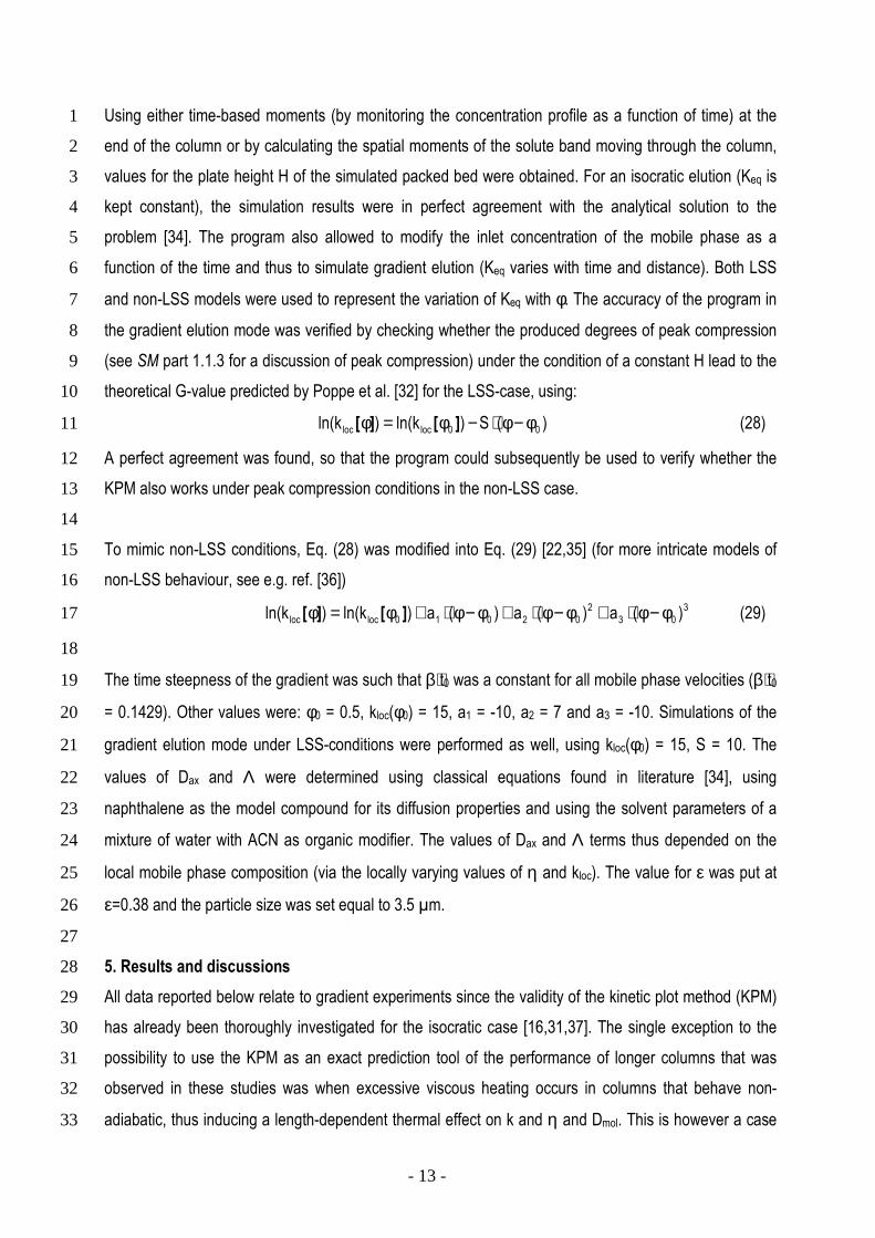
Using either time-based moments (by monitoring the concentration profile as a function of time) at the 1

end of the column or by calculating the spatial moments of the solute band moving through the column, 2

values for the plate height H of the simulated packed bed were obtained. For an isocratic elution (Keq is 3

kept constant), the simulation results were in perfect agreement with the analytical solution to the 4

problem [34]. The program also allowed to modify the inlet concentration of the mobile phase as a 5

function of the time and thus to simulate gradient elution (Keq varies with time and distance). Both LSS 6

and non-LSS models were used to represent the variation of Keq with φ. The accuracy of the program in 7

the gradient elution mode was verified by checking whether the produced degrees of peak compression 8

(see SM part 1.1.3 for a discussion of peak compression) under the condition of a constant H lead to the 9

theoretical G-value predicted by Poppe et al. [32] for the LSS-case, using: 10

)(S)kln()kln( 00locloc φ−φ⋅−φ=φ ][][ (28) 11

A perfect agreement was found, so that the program could subsequently be used to verify whether the 12

KPM also works under peak compression conditions in the non-LSS case. 13

14

To mimic non-LSS conditions, Eq. (28) was modified into Eq. (29) [22,35] (for more intricate models of 15

non-LSS behaviour, see e.g. ref. [36]) 16

3

03

2

02010locloc )(a)(a)(a)kln()kln( φ−φ⋅+φ−φ⋅+φ−φ⋅+φ=φ ][][ (29) 17

18

The time steepness of the gradient was such that β⋅t0 was a constant for all mobile phase velocities (β⋅t0 19

= 0.1429). Other values were: φ0 = 0.5, kloc(φ0) = 15, a1 = -10, a2 = 7 and a3 = -10. Simulations of the 20

gradient elution mode under LSS-conditions were performed as well, using kloc(φ0) = 15, S = 10. The 21

values of Dax and Λ were determined using classical equations found in literature [34], using 22

naphthalene as the model compound for its diffusion properties and using the solvent parameters of a 23

mixture of water with ACN as organic modifier. The values of Dax and Λ terms thus depended on the 24

local mobile phase composition (via the locally varying values of η and kloc). The value for ε was put at 25

ε=0.38 and the particle size was set equal to 3.5 µm. 26

27

5. Results and discussions 28

All data reported below relate to gradient experiments since the validity of the kinetic plot method (KPM) 29

has already been thoroughly investigated for the isocratic case [16,31,37]. The single exception to the 30

possibility to use the KPM as an exact prediction tool of the performance of longer columns that was 31

observed in these studies was when excessive viscous heating occurs in columns that behave non-32

adiabatic, thus inducing a length-dependent thermal effect on k and η and Dmol. This is however a case 33

- 14 -

wherein also the theoretical plate height concept looses its meaning as a column length-independent 1

measure for the band broadening. In the present study, using a still air oven and either an instrument 2

maximally delivering 600 bar or columns with the same pressure limit, such high pressure effects are still 3

mostly insignificant [31,38]. 4

5

Fig. 1 (and more precisely the full line arrow) shows the transformation of the experimentally measured 6

peak capacity to the corresponding KPL. Using the implicit KPM, the establishment of the KPL-curve was 7

straightforward. First, the peak capacity was determined for each considered experimental flow rate 8

using the piece-wise mode np-definition given by Eq. (4). This lead to the fixed length kinetic plot curve 9

represented by the open data symbols shown in Fig. 1. The KPL-curve was then readily obtained by 10

using Eq. (18) and the experimentally determined set of λ-values (calculated using Eq. (14)). The 11

approach of calculating the peak capacity using the piecewise mode of Eq. (4) is illustrated more clearly 12

in Cabooter et al. [25] for the case of an isocratic separation. If preferred, the construction of both the 13

fixed length KP and the KPL can also be based on the average peak width (i.e. by using Eqs. (5-6) 14

instead of Eq. (4)). 15

16

Whereas Fig. 1 reports the peak capacity np, the expressions given in Table 1 show that it is equally well 17

possible to plot the KPL-curve in terms of the N- or σt-value of an individual component, or even in terms 18

of the Rs-value of the critical pair. 19

20

The horizontal dashed arrow represents the transformation according to the max(np or N) with fixed tR-21

optimization (see SM: Part 2.1, case 1 or 2). The vertical dashed arrow represents a transformation 22

according to the min(tR) with fixed np or N-optimization (see SM: Part 2.1, case 3). The full line arrow 23

corresponds to the data transformation described by Eqs. (16) and (18), i.e., by keeping u0-constant. The 24

transformation shown in Fig. 1 is similar to that of Fig. 2 of Eeltink et al. [39], where the physical 25

interpretation of a kinetic plot as being the result of a column length rescaling was already given. An 26

illustration of the data transformation from the experimentally measured gradient (H,u0)-data to the KPL-27

curve is given in the SM (Part 2.4), also showing that the explicit KPM-expressions give the same result 28

as the implicit expression. 29

30

The u0=constant-transformation also constitutes the only way to preserve the experimentally determined 31

band broadening information during a point-by-point transformation. The latter is a key feature of the 32

kinetic plot method (KPM) [16], because it allows to treat the relation between H (or np or σt) and u0 as 33

- 15 -

an unknown. This circumvents the need to select a plate height model and to fit this to the experimental 1

data, as is done in the kinetic plot methods that are based on a numerical optimization routine 2

[10,12,14,15]. Doing the transformation on a point-by-point basis, each bit of experimental band 3

broadening information is fully preserved and does not risk to be eliminated by the fitting process. This is 4

especially advantageous under gradient elution conditions, as there is up to date no real good model 5

available to fit a gradient plate height curve. All newly proposed kinetic plot expressions developed in the 6

present study rely on this point-by-point data transformation principle. The fitted curves added to the 7

figures are only there for visualization or interpolation purposes, which have furthermore also been 8

obtained by first fitting the experimental plate height curve and then transforming each data point of this 9

fitted curve in a point-by-point way. The point-by-point transformation can be very easily implemented in 10

a spreadsheet program such as Microsoft® Excel, as is illustrated in the SM (Part 2.4, Fig. S-4). 11

12

The key test for the validity of the KPM is that it should yield a KPL-curve that is independent of the 13

length of the column that was used to determine the experimental data it is based on. This was verified 14

by comparing the band broadening under gradient conditions in 3 different column lengths (resp. 1, 2 15

and 4 coupled columns, each with a length of 15 cm). To satisfy the conditions needed to obtain a 16

column-length independent elution window (see SM, 2.3), the measurements in the different column 17

lengths were conducted by applying the same φ-history, i.e., by keeping φ0, tdelay/t0 and β⋅t0 constant, 18

implying for example that β was halved if the column length was doubled. This also corresponds to the 19

approach adopted by Wang et al. [40] and Zhang et al. [10]. As can be noted from Fig. 2 (showing both 20

the total sample based peak capacity as well the individual peak capacities calculated for each 21

component separately), there is a good overlap of the KPL-data points originating from experiments 22

conducted in columns with different length, hence providing an experimental proof for the fact that the 23

currently proposed KPM is valid under gradient elution conditions. The agreement of the KPL-data points 24

originating from the different length columns is equally good for the individual components and the entire 25

sample (total np). Again, exactly the same KPL-curves were obtained starting using either the implicit or 26

the explicit KPM. 27

28

Fig. 3 investigates the effect of gradient steepness on the degree of overlap of KPL-curves originating 29

from experiments conducted in columns with different length. As can be noted, this overlap remains very 30

good, despite the factor of 8 variation in considered gradient steepness. Similar curves were obtained for 31

the other measured gradient steepness values, but are not shown for the sake of clarity. 32

33

- 16 -

Because the coupled column experiments inevitably have a limited range of velocities over which the 1

plate height curve can be measured (the data points corresponding to the 4-column systems in Figs. 2 2

and 3 for example do not leave the B-term dominated regime of the plate height curves), the column 3

length-independency of the KPL was also verified numerically, for a wide set of different parameters (see 4

Experimental and numerical procedures). Three different columns lengths were considered (2.5, 5 and 5

10cm) and 8 different u0 velocities in the range of 0.5 to 14.3 mm/s. Fig. 4 shows an example of the 6

perfect overlap that was obtained in all investigated cases. Similar simulations using different parameters 7

for k0, φ0, dp and the k-dependency on φ all resulted in the same overlapping results (results not shown 8

here). This perfect overlap confirms that the presently proposed KPM-expressions are independent of 9

the length of the column wherein the experimental data were collected, even under conditions of peak 10

compression in both LSS or non-LSS conditions. The key to this fortunate behaviour is that the 11

conditions needed to obtain the same peak compression (i.e., keeping the same φ-history) are the same 12

as those needed to keep the same elution window (see SM, part 1.1.3). However, deviations from the 13

column length-independent behaviour might occur when ultra-high pressure effects occur in columns that 14

do not behave perfectly adiabatically or isothermally, or when other length-dependent band broadening 15

sources are present (for more detailed information: see Part 2.3 of the SM). 16

17

The practical use of the KPM in gradient elution is illustrated in Fig. 5, showing that the KPM can be used 18

to evaluate what packing material (e.g. particle size or morphology) and operating conditions (e.g. 19

temperature or gradient steepness) can deliver a desired efficiency of peak capacity in the shortest 20

possible time [41]. This was already shown in isocratic elution to select the system the best suited to 21

reach an efficiency of 100000 plates in a given time [37]. The effect of the system dwell volume was 22

taken into account by keeping tdelay/t0 constant in the gradient programming for the different column 23

lengths. 24

25

Fig. 5 shows that for an operating pressure of 400 bar, and for the given gradient steepness, a peak 26

capacity np of 100 is reached in shortest time (i.e. in 9.3 minutes) using 1.8µm particles, np = 150 using 27

3.5µm particles (47.4 min.) and np = 250 using 5µm particles (around 4.5 hours). Now extrapolating this 28

data to an operating pressure of 1000 bar (making the assumption there would be packing materials and 29

columns able to withstand this operating pressure), it is demonstrated that, as expected, the 1.8µm is 30

still the best material to reach np = 100 (now possible in 4.9 minutes), but is now also the optimal 31

particles choice to reach a peak capacity of 150 (in 18.9 minutes). The use of 3.5µm particles are now 32

the best choice to reach np = 250 (around 2.3 hours) and 5µm particles only become advantageous for 33

- 17 -

peak capacities above np = 325. Considering the 1000-bar data shown in Fig. 5, it has to be noted that 1

these are only an extrapolation and are hence prone to errors due to the influence of pressure on the 2

physico-chemical properties of both solvent and solute [38] and the effect of viscous heating [37]. The 3

amplitude of these effects is however limited [37,38] in adiabatic or quasi adiabatic conditions (still air 4

oven) as were used in these experiments. 5

6

6. Conclusions 7

The kinetic plot method, originally developed for isocratic separations [16], has been extended to 8

gradient elution separations by establishing a theoretical framework that allows to directly draw the 9

kinetic performance limit (KPL) curve of a given separation medium directly from a set of measurements 10

of the flow rate (or u0 or the t0-time or the tR-time) and the separation quality (band width, band standard 11

deviation σt, critical pair resolution Rs, column efficiency N, peak capacity np) conducted on a column 12

with a given length. The obtained KPL-curve is valid for the sample and mobile phase conditions that 13

were used to collect the column performance data and connects all operating points at which the tested 14

separation medium achieves its best possible kinetic performance, i.e., achieves a given separation 15

quality in the shortest possible time or achieves the best possible separation quality in a given time. In 16

fact, the individual data points on the KPL-curve relate to a series of columns with a different length, but 17

operated at the maximally available or allowable pressure, as this is the necessary and sufficient 18

condition for a column to yield a point lying on the KPL-curve. 19

20

The established theoretical framework covers both isocratic and gradient elution conditions, and leads to 21

either a set of explicit or a set of implicit expressions. Both approaches lead to the same KPL-curves 22

(even if the former would be based on an inaccurate estimate of kelut). The implicit expressions are 23

however much simpler to use (cf. Eqs. (15-22)), as they are directly based on the fact that the kinetic plot 24

method simply corresponds to a column length rescaling (cf. the use of the column length rescaling 25

factor λ). This λ-factor needs to be determined for each individual data point on the KPL-curve. This is 26

however a trivial exercise because λ in principle simply corresponds to the ratio of the column pressure 27

for which the KP-curve will be established and the column pressure read-out for the flow rate for which 28

the KPL-data point is to be calculated. As a consequence, the method can be readily implemented in any 29

simple spread-sheet program. A possible correction to λ is needed if the viscosity of the mobile phase 30

liquid changes with the applied pressure (because of the pressure-dependency of η and because of the 31

viscous heating effect). In this case Eq. (S-62) (see SM) needs to be applied, but this is not 32

fundamentally more difficult. 33

- 18 -

1

In principle, the established KPL-curve yields exact predictions of the separation performance one can 2

expect in any column with a different length but operated at the maximal pressure, provided these 3

different length columns are operated under the same conditions (same relative mobile phase history, 4

same type sample components and same operating temperature) and provided the measured plate 5

heights are not length-dependent [21,31,42]. Viscous heating effects in columns that behave perfectly 6

adiabatic can be exactly accounted for. It is only when systems have a non-adiabatic thermal behaviour 7

that the possibility to go from an experimental set of measurements on one column length to an exact 8

prediction of the performance in another column length is compromised (in addition to other length 9

dependent error sources such as extra-column band broadening or packing effects). 10

11

However, the obtained KPL-curve can even in these cases still be used as a prediction of the (virtual) 12

performance one would obtain provided these effects would not occur. Under this assumption, the kinetic 13

plot can still be used as a universal comparison method for the performance of differently shaped and 14

sized support materials. If one is really after an exact prediction of the kinetic performance in systems 15

marked by a strong viscous heating and with thermal conditions that are far from adiabatic, one will have 16

to accept that the mathematics in these cases become so complex that the best way to establish a 17

kinetic plot simply consists of running the actual experiments, by coupling 1,2,3, etc columns in series 18

and test each combination at the maximal pressure, as was already done by Sandra and co-workers [43-19

45]. Intermediate points can then be determined via interpolation. 20

21

The present analysis has shown that the kinetic plot method remains valid under gradient elution 22

conditions, even though the band width or peak capacity depend on the relative mobile phase history 23

and are prone to peak compression effects. The only consequence of these effects is that the 24

established KPL-curve is only valid provided φ0, the gradient steepness β⋅t0 and tdelay/t0 are maintained 25

constant when the column length is changed. This implies for example that β needs to be halved if the 26

column length is doubled. This condition holds for LSS as well as for non-LSS systems. Although the 27

present study and analysis only considered linear gradient systems, it can be inferred that the general 28

rule concerning the requirement of a constant relative mobile phase history will also hold for non-linear 29

gradients. Special effects such as organic modifier retention or large changes in kloc across the peak 30

width on the validity of the kinetic plot extrapolation will be investigated in a future study. 31

32

- 19 -

As was shown in a practical example, the KPM can now be readily used to determine the best possible 1

particle size to produce a given peak capacity in the shortest time under gradient elution for a fixed 2

gradient steepness. 3

4

Supplementary material 5

Supplementary material (SM) available: This material is available alongside the electronic version of this 6

article. 7

8

9

Acknowledgement: 10

K.B. and D. Ca. gratefully acknowledge a research grant from the Research Foundation – Flanders 11

(FWO Vlaanderen). 12

13 14 References: 15

[1] A.D. Jerkovich, J.S. Mellors, J.W. Jorgenson, J.W. Thompson, Anal. Chem. 77 (2005) 6292. 16

[2] K.D. Patel, A.D. Jerkovich, J.C. Link, J.W. Jorgenson, Anal. Chem., 76 (2004) 5777. 17

[3] H. Chen, Cs. Horvath, J. Chromatogr. A, 705 (1995) 3-20. 18

[4] J. Thompson, P. Carr, Anal. Chem., 74 (2002) 1017. 19

[5] B. Yan, J. Zhao, J.S. Brown, J. Blackwell, P. Carr, Anal. Chem., 72 (2000) 1253-1262. 20

[6] F. Lestremau, A. Cooper, R. Szucs, F. David, P. Sandra, J. Chromatogr. A, 1109 (2006) 191-196. 21

[7] D. Guillarme, S. Heinisch, J.-L. Rocca, J. Chromatogr. A, 1052 (2004) 39-51. 22

[8] N. Tanaka, H. Kobayashi, K. Nakanishi, H. Minakuchi, N. Ishizuka, Anal. Chem., 73 (2001) 420-429. 23

[9] F. Svec, LC⋅GC Europe, 16 (6a) (2003) 24-28. 24

[10] Y. Zhang, X. Wang, P. Mukherjee, P. Petersson, J. Chromatogr. A, 1216 (2009) 4597–4605. 25

[11] J.C. Giddings, Anal. Chem., 37 (1965) 60-63. 26

[12] J.H. Knox, M. Saleem, J. Chromatogr. Sci. 7 (1969) 614-622. 27

[13] G. Guiochon, Anal. Chem., 53 (1981) 1318-1325. 28

[14] H. Poppe, J. Chromatogr. A, 778 (1997) 3-21. 29

[15] X. Wang, D.R. Stoll, P.W. Carr, P.J. Schoenmakers, J. Chromatogr. A, 1125 (2006) 177–181. 30

[16] G. Desmet, D. Clicq, P. Gzil, Anal. Chem., 77 (2005) 4058-4070. 31

[17] T. Hara, I. Kobayashi, K. Nakanishi, N. Tanaka, Anal. Chem., 78 (2006) 7632-7640. 32

[18] D. Guillarme, E. Grata, G. Glauser, J.-L. Wolfender, J.-L. Veuthey, S. Rudaz, J.Chromatogr. A, 1216 33

(2009) 3232-3243. 34

- 20 -

[19] L.R. Snyder, D.L. Saunders, J. Chromatogr. Sci., 7 (1969) 195-208. 1

[20] L.R. Snyder, J.W. Dolan, J.R. Gant, J. Chromatogr., 165 (1979) 3-30. 2

[21] G. Guiochon, Chromatogr. A, 1126 (2006) 6–49. 3

[22] F. Gritti, G. Guiochon, J. Chromatogr. A, 1145 (2007) 67–82. 4

[23] U.D. Neue, J. Chromatogr. A, 1079 (2005) 153–161. 5

[24] U.D. Neue, J. Chromatogr. A 1184 (2008) 107–130. 6

[25] D. Cabooter, A. de Villiers, D. Clicq, R. Szucs, P. Sandra, G. Desmet, J. Chromatogr. A, 1147 7

(2007) 183. 8

[26] J.C. Giddings, Anal. Chem., 39 (1967) 1027-1028. 9

[27] M. Gilar, U.D. Neue, J. Chromatogr. A., 1169 (2007) 139–150. 10

[28] S. Eeltink, S. Dolman, R. Swart, M. Ursem, P.J. Schoenmakers, J. Chromatogr. A, 1216 (2009) 11

7368-7374. 12

[29] J. Cazes, R.P.W. Scott, Chromatography theory, Marcel Dekker Inc: New York, 2002. 13

[30] U.D. Neue HPLC-Columns—Theory, Technology, and Practice; Wiley-VCH: Weinheim, 1997. 14

[31] D. Cabooter, F. Lestremau, A. de Villiers, K. Broeckhoven, F. Lynen, P. Sandra, G. Desmet, J. 15

Chromatogr. A, 1216 (2009) 3895-3903. 16

[32] H. Poppe, J. Paanakker, M. Bronckhorst, J. Chromatogr., 204 (1981) 77–84. 17

[33] L. R. Snyder, J. W. Dolan., High Performance Gradient Elution, The practical application of the 18

linear-solvent-strength model, Wiley-Interscience: Hoboken, New Jersey, USA, 2007. 19

[34] G. Desmet, K. Broeckhoven, Anal. Chem., 80 (2008) 8076–8088. 20

[35] F. Gritti, G. Guiochon, J. Chromatogr. A, 1212 (2008) 35–40. 21

[36] U. D. Neue, Chromatographia, 63 (2006) S45-S53. 22

[37] D. Cabooter, F. Lestremau, F. Lynen, P. Sandra, G. Desmet, J. Chromatogr. A, 1212 (2008) 23-34. 23

[38] U.D. Neue, M. Kele, J. Chromatogr. A, 1149 (2007) 236-244. 24

[39] S. Eeltink, G. Desmet, G. Vivo-Truyols, G. Rozing, P.J. Schoenmakers, W.Th. Kok, J. Chromatogr. 25

A 1104 (2006) 256-262. 26

[40] X. Wang, W.E. Barber, P.W. Carr, J. Chromatogr. A, 1107 (2006) 139-151. 27

[41] P.W. Carr, X. Wang, D.R. Stoll, Anal. Chem., 81 (2009) 5342-5353. 28

[42] K. Broeckhoven, G. Desmet, J. Chromatogr. A, 1216 (2009) 1325–1337. 29

[43] F. Lestremau, A. Cooper, R. Szucs, F. David, P. Sandra, J. Chromatogr. A, 1109 (2006) 191-196. 30

[44] A. de Villiers, F. Lestremau, R. Szucs, S. Gélébart, F. David, P. Sandra, J. Chromatogr. A, 1127 31

(2006) 60-69. 32

[45] F. Lestremau, A. de Villiers, F. Lynen, A. Cooper, R. Szucs, P. Sandra, J. Chromatogr. A, 1138 33

(2007) 120-131.34

- 21 -

List of symbols: 1

cst constant, [m/s] or [m³/s] 2

C1 concentration in the mobile phase, [mol/m³] 3

C2 concentration in the stationary phase, [mol/m³] 4

Dax lumped axial dispersion coefficient (both A and B-term contribution), [m²/s] 5

i i-th elution component, [/] 6

F flow rate, [m³/s] 7

H plate height, see Eq. (1), [m] 8

k phase retention factor, defined as (tR-t0)/t0, [/] 9

kelut effective phase retention factor at point of elution, [/] 10

kloc local phase retention factor, [/] 11

Kv permeability, based on u0, [m²] 12

Keq whole particle based equilibrium constant [34], [/] 13

L column length, [m] 14

n number of components in sample, [/] 15

N actual column plate count [/], see Eq. (1), [/] 16

Neff effective plate number, defined as Neff = N⋅k²/(1+k)², [/] 17

np peak capacity, [/] 18

Rs,i separation resolution of peaks i-1 and i, also see Eq. (S-57) in the SM, [/] 19

S linear solvent strength parameter, see Eq. (28), [/] 20

t time, [/] 21

t0 column residence time for an unretained marker (k=0), [s] 22

tR column residence time for an retained component, [s] 23

u0 unretained species velocity, [m/s] 24

ui interstitial velocity, [m/s] 25

w peak width, defined as 4⋅σt, [s] 26

x actual axial position or coordinate in column, [m] 27

x' dimensionless axial position, x/L [/] 28

∆P pressure drop, [Pa] 29

30

Greek symbols: 31

β time steepness of the gradient, see Eq. (11), [1/s] 32

ε external porosity, [/] 33

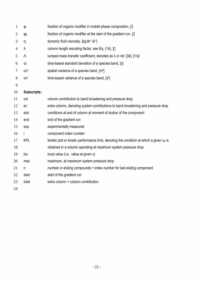
- 22 -

φ fraction of organic modifier in mobile phase composition, [/] 1

φ0 fraction of organic modifier at the start of the gradient run, [/] 2

η dynamic fluid viscosity, [kg⋅m-1⋅s-1] 3

λ column length rescaling factor, see Eq. (14), [/] 4

Λ lumped mass transfer coefficient, denoted as λ in ref. [34], [1/s] 5

σt time-based standard deviation of a species band, [s] 6

σx2 spatial variance of a species band, [m²] 7

σt2 time-based variance of a species band, [s²] 8

9

Subscripts: 10

col column contribution to band broadening and pressure drop 11

ec extra column, denoting system contributions to band broadening and pressure drop 12

elut conditions at end of column at moment of elution of the component 13

end end of the gradient run 14

exp experimentally measured 15

i component index number 16

KPL kinetic plot or kinetic performance limit, denoting the condition at which a given u0 is 17

obtained in a column operating at maximum system pressure drop 18

loc local value (i.e., value at given x) 19

max maximum, at maximum system pressure drop 20

n number or eluting compounds = index number for last eluting component 21

start start of the gradient run 22

total extra column + column contribution 23

24

- 23 -

Figure Captions 1

2

Figure 1. Data transformation according to the implicit kinetic plot expression (Eq. (18)), starting from the 3

measured sample peak capacity (fixed length kinetic plot, open symbols) and transforming it into its 4

corresponding kinetic performance limit for ∆Pmax = 600 bar (free length kinetic plot, full symbols). The 5

meaning of the arrows is given in the text. Experimental conditions: gradient elution (ACN/H2O) with φ0 = 6

0.5 and β⋅t0 = 0.016 on a single (15cm) HALO column. Please note that different u0-data points are 7

obtained with a different β, so as to keep a constant β⋅t0. 8

9

Figure 2. Verification of the overlap of KPL-curves that originate from experiments conducted in columns 10

with different length for the three different components (open symbols; benzene: green curve, 11

naphthalene: red curve, phenanthrene: black curve) and the three considered column lengths (15 cm: ◊◊◊◊; 12

30cm: ∆∆∆∆; 60cm: ). In addition, the KPL for the total peak capacity (full symbols; blue curve, calculated 13

by Eq. (14) and (18)) has been given as well. 14

15

Figure 3. Verification of the overlap of the KPL curves originating from experiments conducted in 16

columns with different length (15 cm: ◊◊◊◊; 30cm: ∆∆∆∆; 60cm: ) for various degrees of gradient steepness 17

(β⋅t0 = 0.008, 0.016 and 0.064). Please note that β was changed inversely proportional to L in order to 18

keep the same β⋅t0 and that the gradient programming was adapted to ensure a constant tdelay/t0. 19

20

Figure 4. KPL-curves based on the numerical simulation of the migration of a component (with the 21

diffusion properties of naphthalene) through columns with different lengths in gradient elution (2.5 cm: ◊◊◊◊; 22

5cm: ∆∆∆∆; 10cm: ). The black curves denote a component with non-LSS behavior, the green curve 23

denotes one with LSS behavior. 24

25

Figure 5. KPL-curves for 3 different particle sizes (5µm: ■, 3.5µm ♦and 1.8µm ▲) in gradient elution 26

(MeOH/H2O) with φ0 = 0.45 and β⋅t0 = 0.020 of the paraben mixture on the Zorbax columns. Full curves 27

and symbols denote ∆Pmax = 400 bar, dashed curves and open symbols denote an extrapolation to 28

∆Pmax = 1000 bar. 29

30

31

32

- 24 -

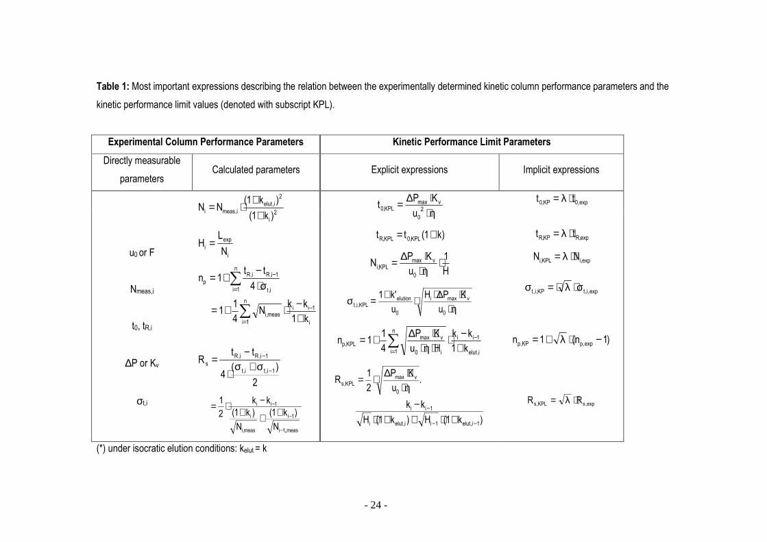
Table 1: Most important expressions describing the relation between the experimentally determined kinetic column performance parameters and the

kinetic performance limit values (denoted with subscript KPL).

Experimental Column Performance Parameters Kinetic Performance Limit Parameters

Directly measurable

parameters Calculated parameters Explicit expressions Implicit expressions

u0 or F

Nmeas,i

t0, tR,i

∆P or Kv

σt,i

2

i

2

i,elut

i,measi)k1(

)k1(NN

++

⋅=

i

exp

iN

LH =

∑

∑

=

−

=

−

+−⋅+=

σ⋅−

+=

n

1i i

1iimeas,i

n

1i i,t

1i,Ri,R

p

k1

kkN

4

11

4

tt1n

2

)(4

ttR

1i,ti,t

1i,Ri,R

s−

−

σ+σ⋅

−=

meas,,1i

1i

meas,i

i

1ii

N

)k1(

N

)k1(

kk

2

1

−

−

−

+++−⋅=

η⋅⋅∆=

2

0

vmaxKPL0,

u

KP t

)k1(t t KPL0,KPLR, +=

H

1

u

KP N

0

vmaxKPLi, ⋅

η⋅⋅∆=

η⋅⋅∆⋅⋅+=σ

0

vmaxi

0

elutionKPL,i,t

u

KPH

u

'k1

∑=

−

+−⋅

⋅η⋅⋅∆+=

n

1i i,elut

1ii

i0

vmaxKPL,p

k1

kk

Hu

KP

4

11n

)k1(H)k1(H

kk

.u

KP

2

1R

1i,elut1ii,eluti

1ii

0

vmaxKPL,s

−−

−

+⋅++⋅−

η⋅⋅∆⋅=

exp0,KP0, t t ⋅λ=

expR,KPR, t t ⋅λ=

expi,KPLi, N N ⋅λ=

exp,i,tKP,i,t σ⋅λ⋅=σ

)1n(1n exp,pKP,p −⋅λ+=

exp,sKPL,s RR ⋅λ=

(*) under isocratic elution conditions: kelut = k

- 25 -

Figure 1

100

1000

10000

100000

10 100 1000

np

t R (s)

- 26 -

Figure 2

10

100

1000

10000

100000

10 100 1000

k = 3 k = 6.5 k=11.3

- 27 -

100

1000

10000

100000

10 100 1000

Figure 3

- 28 -

Figure 4

10

100

1000

10000

100000

10 100 1000

- 29 -

Figure 5

1

10

100

1000

10000

100000

10 100 1000

- 30 -

Supplementary Material

The kinetic plot method applied to gradient chromatography: theoretical framework and experimental validation

K. Broeckhoven1, D. Cabooter1, F. Lynen2, P. Sandra2 and G. Desmet1,*

(1) Vrije Universiteit Brussel, Department of Chemical Engineering, Pleinlaan 2, 1050 Brussels, Belgium

(2) Dept. of Organic Chemistry, Universiteit Gent, Krijgslaan 281 S4-Bis, 9000 Gent, Belgium

Abstract

The present supplementary material contains a section on the background theory of column performance in isocratic and gradient elution and the description of the gradient plate height concept (Part 1). In addition, the concept of a constant “relative mobile phase history” is introduced, which is necessary to define a gradient plate height and to apply the kinetic plot method (KPM) in gradient elution. Experimental results illustrating the use of the gradient plate height concept are given as well. Part 2 gives a detailed derivation of the conditions needed to operate at the kinetic performance limit (KPL), i.e. the conditions needed to achieve a given N or np in the shortest possible time tR, or, equivalently, to achieve a maximal N or np in a given time tR (Problem 1). It is also shown that calculating the KPL on the basis of a set of experimentally measured column performance data should best be done via a data transformation that leaves the u0-velocity corresponding to each data point invariant, and that this can be done very simply by introducing a column length rescaling factor (Problem 2)., In addition, it is investigated under which conditions the kinetic performance limit curve is independent of the length of the column in which the experimental column performance data were obtained (Problem 3). Finally, the transformations underlying the kinetic plot method (KPM) are illustrated and visualized.

Table of contents

Part 1: Background theory on column performance and use of plate heights in gradient elution

1.1) Theory on column performance in gradient elution S2

1.2) Illustration of the use of the plate height concept in gradient elution S9 Part 2: Necessary conditions underlying the validity of the kinetic performance limit-curve

2.1) Problem-1. Which condition should be satisfied to operate a given chromatographic system (with undetermined length) at its optimal kinetic performance limit, i.e., achieve a maximal N or np in a given time tR, or, equivalently, achieve a given N or np in the shortest possible time tR S12

- 31 -

2.2) Problem-2. How can the column performance that is measured at a given mobile phase velocity u0 be translated into a point falling on the optimal kinetic performance limit? S15

2.3) Problem-3. Is the optimal kinetic performance limit independent of the length of the column in which the experimental column performance data were obtained? S19

2.4) Illustration of the transformations underlying the KPM in gradient elution S23

- 32 -

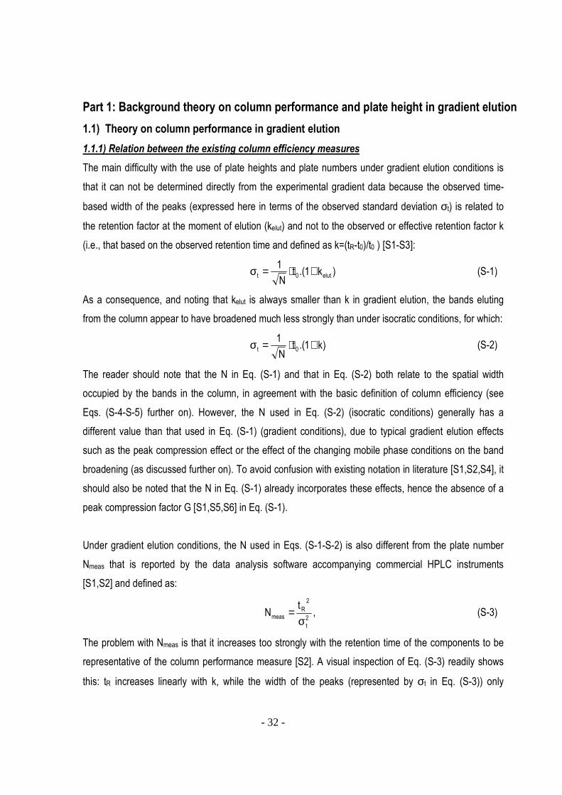
Part 1: Background theory on column performance and plate height in gradient elution

1.1) Theory on column performance in gradient elution

1.1.1) Relation between the existing column efficiency measures

The main difficulty with the use of plate heights and plate numbers under gradient elution conditions is

that it can not be determined directly from the experimental gradient data because the observed time-

based width of the peaks (expressed here in terms of the observed standard deviation σt) is related to

the retention factor at the moment of elution (kelut) and not to the observed or effective retention factor k

(i.e., that based on the observed retention time and defined as k=(tR-t0)/t0 ) [S1-S3]:

)k1.(tN

1elut0t +⋅=σ (S-1)

As a consequence, and noting that kelut is always smaller than k in gradient elution, the bands eluting

from the column appear to have broadened much less strongly than under isocratic conditions, for which:

)k1.(tN

10t +⋅=σ (S-2)

The reader should note that the N in Eq. (S-1) and that in Eq. (S-2) both relate to the spatial width

occupied by the bands in the column, in agreement with the basic definition of column efficiency (see

Eqs. (S-4-S-5) further on). However, the N used in Eq. (S-2) (isocratic conditions) generally has a

different value than that used in Eq. (S-1) (gradient conditions), due to typical gradient elution effects

such as the peak compression effect or the effect of the changing mobile phase conditions on the band

broadening (as discussed further on). To avoid confusion with existing notation in literature [S1,S2,S4], it

should also be noted that the N in Eq. (S-1) already incorporates these effects, hence the absence of a

peak compression factor G [S1,S5,S6] in Eq. (S-1).

Under gradient elution conditions, the N used in Eqs. (S-1-S-2) is also different from the plate number

Nmeas that is reported by the data analysis software accompanying commercial HPLC instruments

[S1,S2] and defined as:

2

t

2

Rmeas

tN

σ= , (S-3)

The problem with Nmeas is that it increases too strongly with the retention time of the components to be

representative of the column performance measure [S2]. A visual inspection of Eq. (S-3) readily shows

this: tR increases linearly with k, while the width of the peaks (represented by σt in Eq. (S-3)) only

- 33 -

increases according to the much smaller kelut. Since furthermore the difference between k and kelut grows

with increasing k, the value of Nmeas continuously increases with increasing k, hence suggesting the

column quality improves with increasing residence time of the employed components. The Nmeas-value

therefore is a futile column performance measure and provides no direct information on the true column

efficiency, i.e., that related to the spatial width occupied by the bands in the column. To show that this

"true" efficiency corresponds to the N-value already defined in Eq. (S-1), it is instructive to start from the

well-established relation [S2]:

2

elut

02

t

2

elut

2

t

2

xk1

uu

+⋅σ=⋅σ=σ (S-4)

wherein σx2 is the spatial variance of the band, σt

2 is the time-based variance of the band, u0 the velocity

of an unretained marker and uelut the retained species velocity at the point of elution (uelut=u0/[1+kelut]).

Using now the well-established relationship between N and the spatial variance (N=L2/σx2), Eq. (S-4) can

be transformed into:

2

elut2

t

2

0

2

x

2

)k1(tL

N +⋅σ

=σ

= (S-5)

which can readily be rewritten into the expression given in Eq. (S-1).

As already mentioned, the true gradient N is seldom used because it can only be calculated from Nmeas

provided the value of kelut is known, as can readily be seen after combining Eqs. (S-3) and (S-5)):

2

2

elut

2

t

2

R

2

2

elutmeas

)k1(

)k1(t

)k1(

)k1(NN

++

⋅σ

=+

+⋅= (S-6)

If the linear solvent strength (LSS)-model [S1,S7] (see Eq. S-19 or Eq. 28 in main article) applies, the

relation between kelut and k can be predicted, so that the unknown kelut on the right hand side of Eq. (S-6)

can be expressed in terms of k:

2

2

ktS

0

tSk

2

t

2

R

2

2

ktS

0

tSk

meas)k1(

etS

1e1

t

)k1(

etS

1e1

NN0

0

0

0

+

⋅⋅β⋅−+

⋅σ

=+

⋅⋅β⋅−+

⋅=⋅⋅β⋅

⋅β⋅⋅

⋅⋅β⋅

⋅β⋅⋅

(S-7)

wherein S is the linear solvent strength parameter of a given component (see Eq. (S-19) further on) and

β the time steepness of the gradient (β=[φtend-φ0]/[tend-tstart]). Eq. (S-7) is only valid if the dwell volume of

the system is small compared to the column dead time or if the value of k at the initial mobile phase

- 34 -

composition is large. In the latter case Eq. (S-7) can further be simplified as shown in [S7]. In addition, as

has been reported numerous times, the linear solvent strength (LSS) assumption might lead to important

errors on the value of kelut [S4,S8-S10]. The value of kelut can also be calculated using numerical

procedures [S5] or by measuring the value of k in isocratic elution with the mobile phase composition

φelut at which the component elutes during the gradient, because φelut can in principle be directly

calculated from the gradient parameters φ0 and β. Determining φelut is however also prone to errors,

since it involves accurately determining the system dwell volume, the column dead time and the possible

retention of the organic modifier [S5]. Under isocratic conditions, there is no need to distinguish between

the true and the measured plate number, for in this case k=kelut, so that the second factor on the right

hand side of Eqs. (S-6) and (S-7) becomes unity.

1.1.2) Conditions to keep the elution pattern independent of the column length

Keeping the same stationary phase and gradient time, but changing the length of the column or the

applied flow rate usually leads to a change of the retention factor of the analytes under gradient elution.

This is a complication which does not exist in isocratic elution and makes the kinetic optimization of

gradient separations more difficult. The present section is concerned with finding the necessary and

sufficient conditions to maintain the same effective retention factor k when L and F are changed.

Starting from the generally accepted ergodic process assumption and the definition of the local retention

time in chromatography, it can be written that [S5]:

m

loc

s dtk

dt = (S-8)

In case of a linear gradient with delay time tdelay (with tdelay the time elapsing between the injection and the

instant at which the gradient profile reaches the front of the column; note that in the general case tdelay is

equal to tdwell + any additional delay time introduced in the gradient program), the solvent composition at

any point or time in the column is given by:

0)t,x( φ=φ (for t<tdelay+x/u0) (S-9a)

)u/xtt()t,x( 0delay0 −−⋅β+φ=φ (for t>tdelay+x/u0) (S-9b)

Since for any position x we can state that the time spent in the stationary phase is equal to the total time

minus the time needed for the mobile phase to reach that distance, we have ts=t-x/u0, so that Eqs. (S-9a-

b) become:

- 35 -

0s )t( φ=φ for ts<tdelay (S-

10a)

)tt()t( delays0s −⋅β+φ=φ for ts>tdelay (S-

10b)

Integrating now Eq. (S-8), and splitting the left hand side integral in two pieces, one for the constant φ-

part, and one for the linear gradient part, we obtain:

0

t

0m

tt

0loc

s tdtk

dt 00R == ∫∫−

(S-11)

0

t

0m

tt

tdelays0loc

st

00loc

s tdt))tt((k

dt

)(k

dt 00R

delay

delay ==−β+φ

+φ ∫∫∫

− (S-

12)

Introducing subsequently the dimensionless time t'=ts/t0, the φ-history can be rewritten as:

0)'t( φ=φ for t'<tdelay/t0 (S-

13a)

)tt't(t)'t( 0delay00 −⋅β+φ=φ for t'>tdelay/t0 (S-

13b)

while Eq. (S-12) becomes:

( )

1))t/t't(t(k

'dt

)(k

'dt 00R

0delay

0delay t/tt

t/t0delay00loc

t/t

00loc

=−β+φ

+φ ∫∫

− (S-

14)

Introducing an effective retention factor k as k=(tR-t0)/t0, as done in the present study, it follows readily

from Eq. (S-14) that k (appearing in the upper boundary of the integral in the second term on the left hand

side) will be independent of the column length provided the φ0, the product βt0 and the ratio of tdelay/t0 are

kept constant

From this observation, one can directly conclude that, if any change in L or F (both inevitably leading to a

change of t0) is accompanied by a change of tG and tdelay such that βt0 and tdelay/t0 are kept constant, it is

guaranteed that the same elution profile (i.e., same k-values) will be obtained. This of course only holds

- 36 -

provided the retention properties of the stationary phase are independent of L, but this is in most cases a

reasonable assumption.

At this point, it is convenient to introduce the term "relative mobile phase-history" (in short "φ-history") to

denote the change of φ experienced by the components at each given dimensionless position x' (x'=x/L)

in the column. This can be done by noting that dtm=dx/u0 = dx.(t0/L)=t0.dx'. Using this identity in Eq. (S-8),

and introducing now the symbol k(x) to denote the average retention factor experienced by a component

up to a given position x in the column, we can use the identity k(x)=ts(x)/(x/u0) to obtain:

'x/)'x('t)'x(k = (S-

15)

on the one hand, and ∫='x

0loc 'dx)'x(k

'x

1)'x(k (S-

16)

on the other hand. Eq. (S-13) then becomes:

0)'x( φ=φ for x'<tdelay/(kloc(φ0).t0) (S-

17a)

)tt'x).'x(k(t)'x( 0delay00 −⋅β+φ=φ for x'>tdelay/(kloc(φ0).t0) (S-

17b)

Although Eqs (S-16) and (S-17) are not directly analytically solvable (the solution requires an iterative

numerical procedure), their combination can be used to show that linear gradients run with the same

gradient steepness β⋅t0 and with the same φ0 and tdelay/t0 are guaranteed to subject the sample

components to the same φ-value when reaching the same dimensionless position x' (x'=x/L) in the

column, regardless of the value of F or L.

As noted by one reviewer, tdelay can easily be removed from the problem for the case wherein tdelay is only

determined by the dwell time. In this case, it suffices to introduce an injection delay time that exactly

counters the value of tdwell. When some of the tdelay is an essential part of the gradient program this is no

longer possible.

1.1.3) Necessary conditions to keep the plate height independent of the column length

- 37 -

Putting forward that the plate height concept only becomes a useful tool for the analysis and the kinetic

optimization of a given support type when it is length-independent, the present section studies the

conditions that are needed to obtain a length-independent H-value when using the general definition of:

N

LH = (S-

18)

with N given by Eq. (S-5). For isocratic elution, the use of this defintion is rather straightforward, but for

gradient elution this is more complex.

Apart from the problematic measurement of N (see Section 1.1.1), another reason for the reluctance

towards the use of plate numbers or plate heights in gradient elution is that the plate height continuously

varies during the separation due to the changes in both diffusion coefficient and retention factor

complementing the continuous change in mobile phase composition. Whereas the relation between Dmol

and φ is complex and therefore difficult to express, the relation between φ and the local retention

coefficient kloc is usually better known. For example, when the LSS model applies, this relation can be

written as [S1]:

)(S

0locloc0e)(k)(k φ−φ⋅−⋅φ=φ (S-19)

Despite the fact that kloc and Dmol continuously change with the position in the column under gradient

elution conditions, it nevertheless remains perfectly possible to define a local plate height, Hloc, as well as

a global plate height H. Taking the definition of the local plate height [S11], and adopting a general form

of the van Deemter equation to express the dependency of Hloc on the mobile phase velocity u, it is

always possible to put [S7]:

0molloc

0

mollocmol0

2

xloc u)D,k(C

u

)D,k(B)D,u(A

dx

dH ⋅++=σ= (S-20)

Since k and Dmol depend in a deterministic way upon φ, we can also write:

0

0

0

2

xloc u)(C

u

)(B),u(A

dx

d)(H ⋅φ+φ+φ=σ=φ (S-21)

Since the gradient operation also imposes a deterministic relation between the φ-value experienced by

the analytes at a given dimensionless axial position x' (x'=x/L) in the column, Eq. (S-21) can be rewritten

as:

- 38 -

0

0

0loc u)'x(Cu

)'x(B)'x,u(A)'x(H ⋅++= (S-22)

To calculate the total variance of a peak in a column, the local plate height has to be integrated over the

column length L. Introducing the classical definition of H (H=σx2/L), one then obtains for H [S7]:

'dx)'x(HL

H1

0

loc

2

x ⋅=σ= ∫ (S-23)

wherein H represents the total (i.e., column length averaged) plate height. Under isocratic conditions,

Hloc(x') is a constant, so that Eq. (S-23) yields H=Hloc, as expected.

Knowing from Eqs. (S-16)-(S-17) that gradients runs with the same gradient steepness β⋅t0, tdelay/t0 and

φ0 will subject the components to the same φ-value when reaching the same dimensionless position x'

(x'=x/L) in the column, Eq. (S-23) now guarantees that gradient experiments conducted in columns with

different length, but tested with the same component, can be expected to yield the same H, provided

β⋅t0, tdelay/t0 and φ0 are the same. This holds for LSS as well as for non-LSS conditions (the validity of Eq.

(S-19) was not needed in the above argumentation).

An additional effect occurring during gradient elution is the so-called “peak compression” [S6], caused by

the fact that the rear of the solute plug experiences a higher concentration of organic modifier in the

mobile phase than the front of the peak. This in turn causes the front of the band to experience a higher

retention factor than its back and thus a higher retained species velocity for the back of the peak than the

front, causing a reduction in solute band dispersion. Assuming the plate height in the column is constant

during the gradient (and hence neglecting the effects discussed in Eqs. (S-20) to (S-23)), the average

gradient plate height Hgrad is related to the isocratic plate height Hiso by [S1,S5,S6]:

²GHH isograd ⋅= (S-24)

where G is the so-called peak compression factor. It has been shown by Gritti and Guiochon [S5] for the

case of both LSS and non-LSS systems that G only depends on the φ-history, as its value can be

calculated as:

φ⋅φ+φ⋅

⋅β⋅

+= ∫

φ

φ

d)(k

1)(k

t

1

k1

kG

elut

0

3

2

0

2

elut

elut2 ][ (S-25)

- 39 -

It is only when the organic modifier is retained itself or when the local plate height strongly fluctuates

during the gradient, that the dependency on the φ-history is less clear [S5].

For a component following the LSS-model, Eq. (S-25) reduces to [S6]

2

2

)p1(

p3

1p1

²G+

++= with 0

0

0 tS1)('k

)('kp ⋅β⋅⋅

+φφ= (S-26)

Under isocratic conditions, β=0, so that p=0 and G=1, and Eq. (S-24) reduces to Hgrad=Hiso, as expected.

As can readily be seen from Eq. (S-25), G remains invariant as long as the component’s gradient

steepness Sβt0 is kept constant (S⋅β⋅t0 is very often also denoted as ‘b’ or ‘G’ in literature

[S2,S4,S7,S13-S15]). For example, when comparing a gradient run on one column and on two 2 coupled

columns operated at the same mobile phase velocity, the time steepness β has to halve for the coupled

system to have the same compression factor G (since t0,2columns = 2⋅t0,1column). This condition is in fact

identical to that needed to keep the effect of the changing φ on the average plate height constant (cf. Eq.

(S-23)). This of course greatly simplifies the conditions needed to keep a constant H when changing the

column length.

In practice, the plate height under gradient conditions is influenced by even more factors, such as extra-

column peak broadening (which can be measured and corrected for, although a distinction needs to be

made for pre and post-column band broadening, see section 4.1 of the main article), viscous fingering

effects (very steep gradients or step gradients), deviation of the retention behaviour from the LSS model

(which also influences the value of G) and retention of the organic modifier [S5,S7]. One approach to

account for these effects is to incorporate them into in Eqs. (S-24) and (S-23) as demonstrated in

literature [S5]. This however requires complex calculations and a good knowledge of the relation

between H varies and k’, and, in turn, the relation between k’ and φ. A common method used in literature

to circumvent this problem is to lump all these factors into an empirical factor denoted as the J-factor

(see Snyder et al.[S16,S17] for a set of approximate expressions for J and Neue et al. [S4] for a critical

appraisal of this approach)[S4,S16,S17].

)²JG(HH isograd ⋅⋅= (S-27)

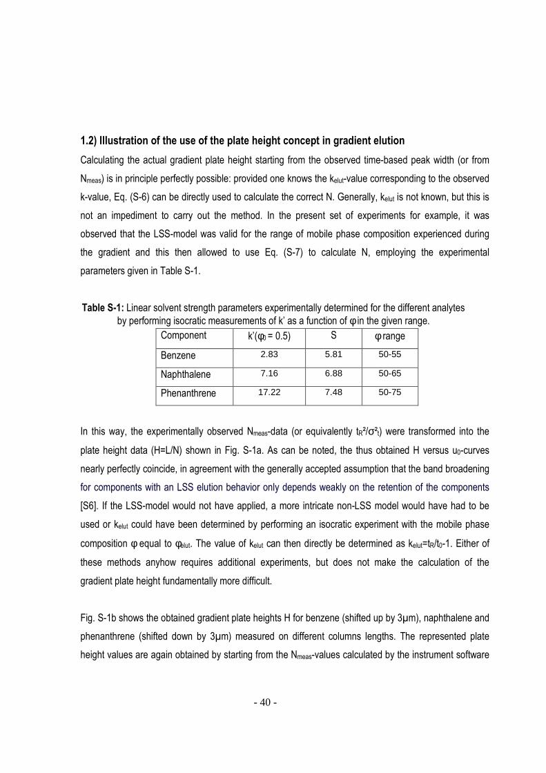
- 40 -

1.2) Illustration of the use of the plate height concept in gradient elution

Calculating the actual gradient plate height starting from the observed time-based peak width (or from

Nmeas) is in principle perfectly possible: provided one knows the kelut-value corresponding to the observed

k-value, Eq. (S-6) can be directly used to calculate the correct N. Generally, kelut is not known, but this is

not an impediment to carry out the method. In the present set of experiments for example, it was

observed that the LSS-model was valid for the range of mobile phase composition experienced during

the gradient and this then allowed to use Eq. (S-7) to calculate N, employing the experimental

parameters given in Table S-1.

Table S-1: Linear solvent strength parameters experimentally determined for the different analytes

by performing isocratic measurements of k’ as a function of φ in the given range.

Component k’(φ0 = 0.5) S φ range

Benzene 2.83 5.81 50-55

Naphthalene 7.16 6.88 50-65

Phenanthrene 17.22 7.48 50-75

In this way, the experimentally observed Nmeas-data (or equivalently tR²/σ²t) were transformed into the

plate height data (H=L/N) shown in Fig. S-1a. As can be noted, the thus obtained H versus u0-curves

nearly perfectly coincide, in agreement with the generally accepted assumption that the band broadening

for components with an LSS elution behavior only depends weakly on the retention of the components

[S6]. If the LSS-model would not have applied, a more intricate non-LSS model would have had to be

used or kelut could have been determined by performing an isocratic experiment with the mobile phase

composition φ equal to φelut. The value of kelut can then directly be determined as kelut=tR/t0-1. Either of

these methods anyhow requires additional experiments, but does not make the calculation of the

gradient plate height fundamentally more difficult.

Fig. S-1b shows the obtained gradient plate heights H for benzene (shifted up by 3µm), naphthalene and

phenanthrene (shifted down by 3µm) measured on different columns lengths. The represented plate

height values are again obtained by starting from the Nmeas-values calculated by the instrument software

- 41 -

and feeding them to Eq. (S-7) and (S-18) using the experimentally determined values of S. The +3 and -

3 µm H-shifts in Fig. S-1 were made for clarity purposes, since otherwise the curves for the 3

components would overlap (similar to the curves shown in Fig. 1a).

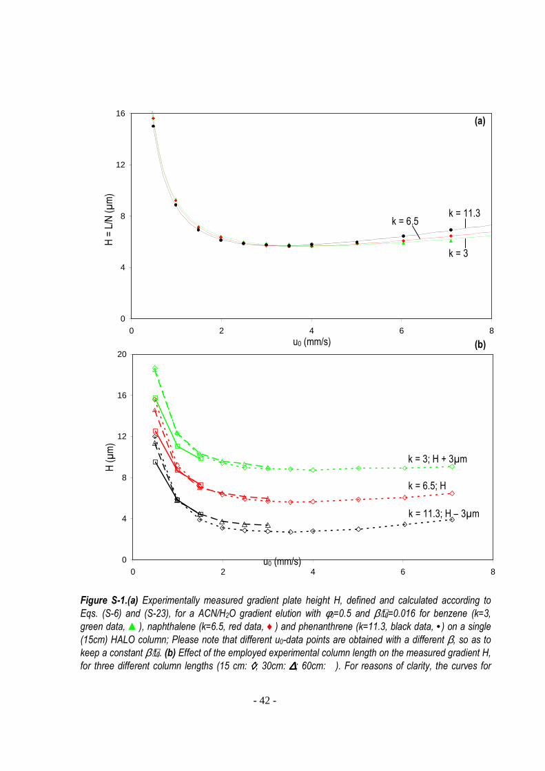
- 42 -

0

4

8

12

16

20

0 2 4 6 8

0

4

8

12

16

0 2 4 6 8

Figure S-1.(a) Experimentally measured gradient plate height H, defined and calculated according to

Eqs. (S-6) and (S-23), for a ACN/H2O gradient elution with φ0=0.5 and β⋅t0=0.016 for benzene (k=3,

green data, ▲), naphthalene (k=6.5, red data, ♦) and phenanthrene (k=11.3, black data, •) on a single

(15cm) HALO column; Please note that different u0-data points are obtained with a different β, so as to

keep a constant β⋅t0. (b) Effect of the employed experimental column length on the measured gradient H,

for three different column lengths (15 cm: ◊◊◊◊; 30cm: ∆∆∆∆; 60cm: ). For reasons of clarity, the curves for

H (µm)

k = 3; H + 3µm

k = 6.5; H

k = 11.3; H – 3µm

(a) H = L/N (µm)

u0 (mm/s) (b)

k = 3

k = 6.5 k = 11.3

u0 (mm/s)

- 43 -

benzene (top, green curves) were shifted upward by 3µm, for phenanthrene (bottom, black curves) downward by 3µm. The naphthalene data (middle, red curve) were not shifted. Same gradient conditions

as in Fig. 1a, keeping β⋅t0 fixed at 0.016 for the different columns lengths, as well as ensuring a constant tdelay/t0.

- 44 -

The plate heights represented in Fig. S-1b have been calculated by adopting the length-independent H-

conditions described in Section 1.1.2. Although the H-data points corresponding to the different column

length systems overlap relatively well (which is needed to confirm H in its status of length-independent

measure), Fig. S-1b also reveals some small differences. These differences can however be attributed to

the fact that the 4 different columns used to construct the coupled column systems inevitably have a

slightly different efficiency, and also have slightly varying t0 and k values. The former results in a spread

on the values for Nmeas, whereas the latter affects the values of both k and kelut. Especially these last two

factors give rise to larger deviations since their contribution to N (or equivalently H) is squared (see Eq.

(S-6)). In addition to the column to column variations, the corrections for the extra column contributions

(and the error on this due to the focusing effect on the head of the column) and the inevitable errors on

the experimental determination of the retention times, also introduces some errors that especially affect

the most weakly retained compounds [S11].

- 45 -

Part 2: Necessary conditions underlying the validity of the kinetic performance limit-curve The curves we commonly denote as kinetic plot curves [S18] in fact represent the kinetic performance

limit of the support and mobile phase conditions under investigation. The present section investigates the

conditions that need to be satisfied to turn a series of efficiency measurements conducted on a single

column into the correct kinetic performance limit of the support filling that column.

Some of the expressions used further on are based on the concept of gradient plate heights. Although

plate heights for gradient elution are not easy to calculate in practice, there is no fundamental impediment

to use them. Furthermore, an approach is presented that circumvents the use of gradient plate heights

(see Eqs. S-43 and following). It should also be noted that when we use the symbol H, this is consistently

defined via eq. (S-18) and holds for isocratic as well as for gradient elution. In the latter case, H also

incorporates the effect of peak compression.

2.1) Problem 1: Which condition should be satisfied to operate a given chromatographic system (with

undetermined length) at its optimal kinetic performance limit, i.e., achieve a maximal N or np in a given

time tR, or, equivalently, achieve a given N or np in the shortest possible time tR?

Theorem 1: Each employed value of the mobile phase velocity u0 leads to a point on the kinetic

performance limit curve provided the u0-value is obtained in a column operating under maximal pressure

conditions (∆P=∆Pmax). This holds for any value of u0 and for gradient as well as isocratic conditions.

Or, for any value of u0: case 1) N = max(N) for a given tR ⇔ ∆P = ∆Pmax (S-28a)

or: case 2) np = max(np) for a given tR ⇔ ∆P = ∆Pmax (S-28b)

or: case 3) tR = min(tR) for a given N or np ⇔∆P = ∆Pmax (S-28c)

Proof:

- Case 1): combining Eqs. (7-9) from main article, it can be shown that:

η⋅⋅∆= v0 Kt

H

PN (S-29)

- 46 -

In fact, Eq. (S-29) is simply a rewritten form of one of the two basic kinetic plot expressions (Eq. (6) of

Desmet et al. [S18]). It shows that finding the maximal N under the constraint of a given t0 corresponds to

finding the conditions for which ∆P1/2/H is maximal, or equivalently, for which H/∆P1/2 is minimal. To find

these conditions we need a way to express how H changes with t0.

For this purpose, we first insert the result of Eq. (S-29) into Eq. (S-18) to calculate the column length and

dividing the obtained expression by t0 to obtain the velocity u0:

η⋅⋅∆=⋅

η⋅⋅∆=⋅=

0

v

0

v0

0

0t

KP

t

HKt

H

P

t

HNu (S-30)

Eq. (S-30) is again nothing but a rewritten form of one of the two basic kinetic plot expressions (Eq. (7) of

Desmet et al. [S18]).

Noting now that the band broadening in most chromatographic systems can be represented by an

expression of the form: 0

0

0 uCu

B)u(AH ⋅++= , (S-31)

we can use the relation between u0 and ∆P to write H as a function of the applied pressure. Noting that

the only variable on the right hand side of Eq. (S-30) is ∆P (t0 is a given constant in the presently

considered case 1), these constants can be incorporated into the A-, B- and C-constants, so that we

obtain a set of new constants A', B' and C':

P'CP

'B)P('AH ∆⋅+

∆+∆= (S-32)

Dividing by ∆P1/2 then yields:

'CP

'B

P

)P('A

P

H +∆

+∆∆=

∆ (S-33)

Inspecting Eq. (S-33), or plotting it (see Fig. S-2), shows that H/∆P1/2 decreases monotonically with

∆P1/2. This holds for any chromatographic system that is characterized by a plate height curve for which

the A-term does not increase stronger than linearly with u0 (or ∆P1/2) and ends in a C-term dominated

regime where H does not increase stronger than linearly with u0 (or ∆P1/2). For example, it can easily be

verified that this holds for the three below models (0<m<1), covering nearly any possible

chromatographic system [S11]:

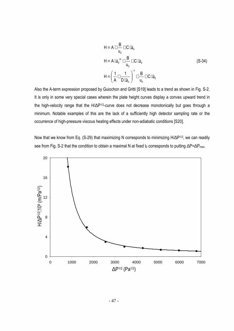
- 47 -

0

4

8

12

16

20

0 1000 2000 3000 4000 5000 6000 7000

0

0

1

0

0

0

m

0

0

0

uCu

B

uD

1

A

1H

uCu

BuAH

uCu

BAH

⋅++

⋅+=

⋅++⋅=

⋅++=

−

(S-34)

Also the A-term expression proposed by Guiochon and Gritti [S19] leads to a trend as shown in Fig. S-2.

It is only in some very special cases wherein the plate height curves display a convex upward trend in

the high-velocity range that the H/∆P1/2-curve does not decrease monotonically but goes through a

minimum. Notable examples of this are the lack of a sufficiently high detector sampling rate or the

occurrence of high-pressure viscous heating effects under non-adiabatic conditions [S20].

Now that we know from Eq. (S-29) that maximizing N corresponds to minimizing H/∆P1/2, we can readily

see from Fig. S-2 that the condition to obtain a maximal N at fixed t0 corresponds to putting ∆P=∆Pmax.

∆P1/2 (Pa1/2)

H/∆P1/2 ⋅1

09 (m/Pa1

/2)

- 48 -

Figure S-2. Plot of H/∆P1/2 (•) versus ∆P1/2 for a fixed value of t0 = 60s based on a set of H,u0 data taken from the experimentally measured values of the isocratic elution of benzene on a single (15cm)

HALO column (φ=0.504, k=2.76).

Since we did not have to make any assumption on u0 or the column length L, this condition holds for any

value of N<Nmax. Nmax is the maximal number of plates that can be obtained with a given

chromatographic system. Nmax is obtained when u0 tends to zero (i.e., Nmax is obtained at the expense of

an infinite separation time). This means that each value of u0 can lead to a point on the kinetic

performance limit, provided it is applied in a column with a length L selected such that ∆P=∆Pmax (see

also problem 2). This conclusion holds for isocratic as well as for gradient elution, as we did not have to

make any assumption about the elution mode to arrive at it. To corroborate this further, it should also be

noted that the integration on the right hand side of Eq. (S-32) does not change the general nature of its

dependency on u0 (or ∆P1/2).

- Case 2): Keeping all ki- and kelut,i-values the same, the expression for np,KPL (see Eq. (S-52) further on)

readily shows that maximizing np corresponds to maximizing the Ni-values appearing in each term of the

summation the right hand side of Eq. (S-52). Since we know from case 1 that the necessary and

sufficient condition to maximize N under the condition of a constant tR or t0 corresponds to operating the

system at maximal pressure, it follows immediately that the same condition will also maximize each

individual term of the summation, so that the total expression for np will also be maximal if ∆P=∆Pmax.

- Case 3): rewriting Eq. (S-29) into:

2

v

0KP

HNt

η⋅∆

⋅= (S-35)

it can readily be seen that minimizing t0 (or tR if k is kept the same) under the constraint of a given N

again corresponds to minimizing H/∆P1/2 (because η, N and Kv are assumed to be constant in Eq. (S-

35)), which in turn corresponds to operating under ∆P=∆Pmax-conditions.

Since Eq. (S-52) shows that constraining np corresponds to constraining N, it again follows that the

∆P=∆Pmax-condition is necessary and sufficient to obtain a minimal t0 or tR for a given np.

- 49 -

2.2) Problem 2: How can the column performance that is measured at a given mobile phase velocity u0

be translated into a point falling on the optimal kinetic performance limit?

Theorem 2: Irrespectively whether a column is operated under gradient or isocratic conditions, the

column performance measured at any given mobile phase velocity u0 can be transformed into a point on

the kinetic performance limit (KPL)-curve provided the mobile phase viscosity (isocratic mode) or mobile

phase viscosity history (gradient mode) and the corresponding plate height are independent of the

column length and provided the given velocity u0 is achieved in a column with maximal length Lmax, i.e.,

by replacing ∆P by ∆Pmax in Eq. (9) (see main article).

when u0 is fixed: ∆P=∆Pmax ⇔ L=Lmax (S-36)

Proof: Since the relation between H and u0 is generally unknown, the only way to preserve the

experimentally observed relation between the band broadening and the mobile phase velocity is to do

the transformation at constant u0 (so that the corresponding H also does not change). Let us now

consider a given column performance data point measured at a given mobile phase velocity u0, i.e., a

data point that is measured by applying a pressure ∆P=∆Pexp in a column with length Lexp. When the

mobile phase velocity u0 and viscosity η are fixed, the only way to transform this data point into a point

falling on the KPL-curve (requiring that ∆P=∆Pmax, see theorem 1) corresponds to maximizing L, i.e., by

putting L=Lmax in Eq. (9) from the main article, because:

η⋅∆⋅

=0

expv

expu

PKL ⇔

η⋅∆⋅=0

maxvmax

u

PKL (S-37)

The direct and linear relation between L and ∆P in Eq. (S-37) obviously holds only under the assumption

that also η is independent of ∆P (see Problem 3 for a discussion of the conditions underlying this

assumption).

The obtained experimental true column efficiency Nexp can also be transformed into a plate height H via:

H

LN

exp

exp = (S-38a)

Similarly, also the t0-time is determined by the column length:

0

exp

exp0,u

L t = (S-38b)

- 50 -

The key-factor to transform the data in Eqs. (S-38a-b) into their corresponding KPL-curve is the plate

height H. Under isocratic conditions, H is a function of the following system variables:

H = Hiso = f(u0,k,Dmol,packing characteristics) (S-39a)

Under gradient conditions, H is a function of the following system variables:

H = Hgrad = f(u0,k,Dmol,packing characteristics, Sβt0,G and J) (S-39b)

In the latter case, some of the variables are also interdependent (e.g., Dmol and Sβt0)

Making now the obvious assumption that the KPL-curve is to be established for the same sample

component(s) and mobile phase conditions as the one for which the experimental data set was obtained,

and further assuming that H and η are independent of the column length and the applied pressure (see

Problem 3), the only pressure-dependent variable in the whole set of kinetic performance determining

expressions (Eqs. (7-9), see main article) is the column length. The only way to impose the ∆P=∆Pmax–

condition needed according to Theorem 1 is then to maximize the column length:

∆P=∆Pmax ⇔ L=Lmax (S-40)

Denoting now the N-value that would be obtained when transforming the experimentally observed N into

a N-value falling on the kinetic performance limit using the symbol NKPL, and using the same subscript

notation for t0, it follows immediately that:

iso

maxKPL

H

L N = and

0

maxKPL0,

u

L t = (S-41)

Replacing now Lmax by the right hand side of second equality in Eq. (S-37), we obtain an explicit

expression for NKPL and t0,KPL (explicit because they directly contain the H-value):

Hu

PK N

0

maxvKPL ⋅η⋅

∆⋅= and 2

0

maxvKPL0,

u

PK t

⋅η∆⋅= (S-42)

The reader will note that the expressions in Eq. (S-42) are identical to those obtained earlier for isocratic

conditions [S18].

Introducing now the so-called column length rescaling factor, defined as:

exp

max

L

L=λ , (S-43)

- 51 -

and via Eq. (S-37) equal to: exp

max

P

P

∆∆=λ , (S-44)

we can also turn the expressions in Eq. (S-31) into a set of implicit expressions (implicit because they do

not directly contain the H-value):

exp

exp

exp

maxKPL N

H

L

L

L N ⋅λ=⋅= and exp0,

0

exp

exp

maxKPL0, t

u

L

L

L t ⋅λ=⋅= (S-45)

Knowing that tR=t0(1+k), and assuming a constant k, a condition that anyhow needs to be made for H to

be length-independent, Eq. (S-45) readily leads to the following explicit and implicit expressions for tR:

)k1(u

PK t

2

0

maxvKPLR, +

⋅η∆⋅= and expR,KPLR, t t ⋅λ= (S-46)

The characterization of the separation efficiency under gradient elution conditions is usually done directly

on the basis of the time-based peak widths (usually translated into the band standard deviation σt).

Combining Eqs. (S-5) and (S-23), σt can however also be directly written as function of the gradient plate

height as:

0

elutt

u

)k1(HL

+⋅⋅=σ (S-47)

Starting from Eq. (S-47) and again replacing L by Lmax in the same way as done in Eqs. (S-42) and (S-

45), we obtain in the explicit form:

0

elut

0

vmaxKPL,t

u

k1H

u

KP +⋅⋅η⋅⋅∆=σ (S-48)

In implicit terms, we obtain:

( ) ( )exp,,t

0

elutexp

exp

max

0

elutmaxKPL,t

u

k1HL

L

L

u

'k1HL σ⋅λ=+⋅⋅⋅=+⋅⋅=σ (S-49)

Here, the beauty and the elegance of the implicit variant of the kinetic plot-expression becomes fully

apparent, as one can directly calculate the band variance at the kinetic performance limit from the

experimentally observed band variance.

- 52 -

Another frequently used performance characteristic is the peak capacity np. Starting from the piecewise-

continuous definition given in Eq. (4) (see main article), Eq. (S-5) and the definition of k (k=tR/t0-1), it can

be found that:

∑∑∑=

−

=

−

=

−

+−⋅⋅+=

+−⋅⋅+=

+−⋅⋅+=

n

1i i

1iimeas,i

n

1i i,elut

1iii

n

1i i,elut

1ii

i

exp

exp,pk1

kkN

4

11

k1

kkN

4

11

k1

kk

H

L

4

11n (S-50)

Wherein np,exp is the experimentally observed peak capacity, and wherein Hi and Nmeas,i respectively are

the plate height and the measured plate number for component i.

Performing the transformation from Lexp into Lmax we can again obtain either an explicit or an implicit

expression for peak capacity one can expect if the support and the operating conditions would be used at

their KPL:

∑=

−

+−⋅⋅

η⋅∆⋅⋅+=

n

1i i,elut

1ii

i0

maxvKPL,p

k1

kk

H

1

u

PK

4

11n (S-51)

or:

∑

∑

∑

∑

=

−

=

−

=

−

=

−

+−⋅⋅λ⋅+=

+−⋅⋅λ⋅+=

+−⋅⋅λ⋅+=

+−⋅⋅⋅+=

n

1i i

1iimeas,i

n

1i i,elut

1iii

n

1i i,elut

1ii

i

exp

n

1i i,elut

1ii

i

exp

exp

max

KPL,p

k1

kkN

4

11

k1

kkN

4

11

k1

kk

H

L

4

11

k1

kk

H

L

L

L

4

11n

(S-52)

which upon inserting the expression for the experimentally observed peak capacity (i.e., that measured in

a column with length Lexp) simply reduces to:

)1n(1n expp,KPL,p −⋅λ+= (S-53)

Using the peak capacity based on the average peak variance (σt,av=wp,av/4), a similar set of expressions

can be derived: exp,av,t

exp,0exp,n,R

exp,p4

tt1n

σ⋅−

+= (S-54)

( ) ( ) ( )KPL,av,t

KPL,0KPL,n,R

exp,av,t

exp,0exp,n,R

exp,av,t

exp,0exp,n,R

KPL,p4

tt1

4

tt1

4

tt1n

σ⋅−

+=σ⋅

λ⋅−+=

λ⋅σ⋅λ⋅−

+= (S-55)

which upon inserting the expression for the experimentally observed peak capacity again reduces to:

- 53 -

)1n(1n expp,KPL,p −⋅λ+= (S-56)

an expression which is identical to Eq. (S-53).

Similarly, we can, starting from the expression for the resolution of a given critical pair:

2

)(4

ttR

1i,ti,t

1i,Ri,R

s−

−

σ+σ⋅

−= (S-57)

write that: ( ) ( ) exp,s

1i,elut1ii,eluti

1iimax

KPL,s Rk1Hk1H

kk

2

LR ⋅λ=

+⋅++⋅−⋅=

−−

− (S-58)

or also: ( ) ( ) ( ) ( )meas,,1i

1i

meas,i

i

1ii

1i

1i,elut

i

i,elut

1iiKPL,s

N

k1

N

k1

kk

2

1

N

k1

N

k1

kk

2

1R

−

−

−

−

−

−

+++−⋅=+

++

−⋅= (S-59)

Since none of the above L=Lmax-transformations relied on the assumption that the elution mode was

isocratic or not, it can be concluded that the established expressions are valid under isocratic as well as

gradient elution conditions.

2.3) Problem 3: Is the optimal kinetic performance limit independent of the length of the column in which

the experimental column performance data were obtained?

Theorem 3: Measurements of N, np or σt versus u0 or t0 conducted on columns with a different length

lead to the same kinetic performance limit curve provided the measurements are conducted with the

same component and the same mobile phase (isocratic elution) or the same mobile phase history

parameters φ0 and gradient steepness β⋅t0 (gradient elution), and provided the pressure- and viscous

heating dependence of H, k and η are properly corrected for and provided adiabatic systems are

considered.

Proof:

The argumentations in theorem 1) and 2) are based on the assumption that H, k and η are length-

independent. These are assumptions that are commonly made in LC. If they hold, a KPL-curve that is

based on the measurements made in a given column with a given length will correctly predict the

- 54 -

performance at maximal pressure in a column with another length. However, conditions exist wherein the

assumption of a length-independent H, k and η is too crude. Below is an overview of the conditions

wherein this is the case.

For the isocratic elution mode, inspection of the variables between the brackets on the right hand side of

Eq. (S-39a) shows that a length-independent H requires that experiments conducted in different column

lengths should be performed with the same components and mobile phase, because this automatically

also leads to the same k and Dmol-conditions. In addition also the packing characteristics should be

length-independent. This assumption can never be perfectly met (an overview of possible length-

depending packing effects was recently given by Guiochon [S3]), but is in many cases an acceptable

approximation. Another length-dependency arises when the measured column performance data contain

a significant extra-column contribution. A correction to the KPL-calculation procedure for the latter case

has been proposed by Heinisch et al. [S21], although this correction is only valid for isocratic

separations. In gradient elution, the analytes elute from the column with a smaller retention factor than

the one they enter the column with. As a consequence, the contribution of the pre-column band

spreading is reduced (focusing effect on the front of the column) the relevant extra-column band

broadening contribution can no longer measured by simply short-circuiting the inlet and outlet connection

tubing. Instead, more elaborate correction methods are needed.

And last but not least, also viscous heating effects can lead to a length-dependency of H [S12,S20].

Under perfectly adiabatic conditions (and with a column wall with a zero axial heat transport), the

transcolumn velocity profile can be assumed to remain perfectly straight under viscous heating

conditions, so that no additional H-contribution is created. The viscous heating might however alter the

local Dmol and kloc values experienced by the components when passing through the column because of

the axial T-gradient that develops. As can be noted from Eq. (S-20), this will lead to a change in H as

compared to the case wherein this axial T-gradient is absent, i.e., in the low pressure case. Under

perfectly adiabatic conditions, this T-gradient is only dependent on the column pressure gradient, via

[S20,S22]:

( )

pC

T1PT

⋅α−⋅∆=∆ (S-60)

- 55 -

Eq. (S-60) implies that the H-values for the low u0-data points (measured at a low ∆P) will be less

affected by an axial T-gradient than the high u0-data (measured at a high ∆P). Since the kinetic plot

method requires that all u0-data points are transformed into a data point at the maximal pressure, it is

straightforward to understand that the extrapolation of a low u0-data point will not contain the same T-

effect one can expect if the same u0 would be obtained in a column operated at the maximal pressure.

Fortunately, the T-effect is countered by the increase in column pressure ∆P (∆P and T have an

opposite effect on kloc and Dmol values). As a consequence, and, as shown both theoretically and

experimentally [S12,S20], this effect remains small for values up to 1000 bar, and probably even up to

2000 bar.

Under isothermal conditions on the other hand, the effect of viscous heating leads to a specific additional

plate height contribution [S23-S25]. This plate height contribution only depends on u0 and not on ∆P, so

that the kinetic plot extrapolation from a low pressure to a high pressure simply preserves the measured

effect and hence properly account for it. In normal bore columns, this additional plate height contribution

however only reaches its constant value after a very long entrance length [S26], so that the plate heights

observed in short columns might also be length-dependent. In addition, the pressure-dependency of k

and Dmol might also introduce an unknown change in H, so that measurements conducted at the same u0

but at different pressure would anyhow lead to a different H. Moreover, since the effect of ∆P is in this

case not countered by an increase in T, the effect of ∆P on H can be expected to be larger in isothermal

than in adiabatic conditions. Fortunately, isothermal conditions are anyhow to be avoided when operating

under viscous heating conditions [S24]. The failure of the KPM under isothermal conditions should

therefore not be considered a too huge problem, as this is not a practically relevant operating condition

anyhow. For cases intermediate between isothermal and adiabatic, an intermediate pressure

extrapolation accuracy can be expected.

The above mentioned limitations on the length-independency of H remain the same in the gradient

elution mode. The only difference (see part I, section a.2) with the isocratic conditions is that now not

only the same mobile phase composition needs to be used at the start (same φ0), but that also the same

gradient steepness βt0 needs to be applied, implying that β needs to be halved when L is doubled

(β=[φtend-φ0]/[tend-tstart]). In addition, also tdelay/t0 needs to be kept constant. Fortunately, this is also the

necessary condition to obtain the same k (see Eq. (S-16-17)) and the same peak compression (see Eq.

- 56 -

(S-25)). It is also the condition leading to the same effective η, as the local η is uniquely determined by

the local φ, so that we can again write an expression that is similar to Eq. (S-23):

'dx)'x(1

0

loc ⋅η=η ∫ (S-61)

with the relation between φ and x' still determined by Eq. (S-17), and hence also only depending on the

value of φ0, tdelay/t0 and β⋅t0.

Similar to the case of a length-independent H, the condition of a constant relative φ-history is not

sufficient to obtain a length-independent η if also pressure and viscous heating effects come into play,

because the viscosity of a liquid is known to be strongly temperature- and pressure-dependent (much

stronger than H in most cases). This can for example be witnessed from Fig. 4 of Mazzeo et al., who

reported measurements of an observed column permeability to describe the effect of ∆P and T on

η [S27]. Fortunately, this effect can be measured experimentally and exactly accounted for, at least in an

adiabatic system. In this case, the viscosity measured at the maximal pressure in any given column

length will always be influenced by the same T-gradient (cf. Eq. (S-60)). As a consequence, the KPL-

curve should be established with the η-value (explicit expressions) or the λ-value (implicit expressions)

measured when ∆P =∆Pmax (i.e., at the highest applied flow rate). In this case, the λ-values for the other

flow rates or velocities can be obtained as follows:

0

max,0

max,umax

maxFu

u

F

F)F(

0⋅λ=⋅λ=λ (S-62)

The fact that the viscosity continuously changes during a gradient elution run and might go through a

maximum does not affect the general validity of this correction, as long as the different column length

systems that correspond to the data points falling on the KPL-curve are subjected to the same mobile

phase history.

In a perfectly isothermal system, the viscosity will only change via its dependency on the pressure, so

that one should again calculate the KPL based on the viscosity observed at the highest experimental

pressure. Eq. (S-62) hence remains valid under isothermal conditions. The correction given by Eq. (S-62)

only becomes inaccurate if the thermal conditions of the system are in between isothermal and adiabiatic

and change with the column length.

- 57 -

Whereas the above discussion has been made for gradient conditions, no assumptions have been made

that would invalidate Eq. (S-62) under isocratic conditions. Eq. (S-62) is hence valid under both isocratic

and gradient elution conditions.

A fully similar argumentation can be made for the column length-independency of k. Since k depends on

both T and ∆P, it is again the experimental k-value measured at ∆P =∆Pmax that will be representative

for all column length systems falling on the KPL-curve, provided the system behaves either perfectly

adiabatic or isothermal. Intermediate situations are again more complex [S12].

Another potential source that can lead to length-dependent plate heights under gradient elution is the

dwell volume (=instrument volume from mobile phase pump till column entrance). This introduces a

delay time tdelay. As noted in Section 1.1.3, the potential length-dependent effect of this delay time on H

can be circumvented by adding an additional delay time in the gradient run program to keep the ratio of

tdelay/t0 constant if the length L changes. The only shortcoming of this correction method is that it is not

possible to give the same φ-history for columns shorter than the original one (since the dwell volume can

normally not be reduced). There is however a more elegant method to eliminate the effect of the dwell

volume on the gradient separation, if the HPLC instrument permits this, and that is a delayed injection

[S28]. In this operating method, the mobile gradient is run as normal but the injection is halted till the

pump has pumped a mobile phase volume equal to the dwell volume. This method is also convenient if

the compared columns have a different inner diameter. In the presently experimentally investigated case,

the overall effect introduced by the dwell volume on the observed peak capacity was however small (i.e.,

only small deviations were observed when performing the gradient method with or without correction for

the dwell volume).

2.4) Illustration of the transformations underlying the gradient KPM

Fig. S-3 relates to the phenantrene data already shown in Fig. S-1 (black data points) and shows the

data transformation (see added full line arrows) according to the explicit kinetic plot expressions, going

from an experimental plate height plot (Fig. S-3a) to the corresponding kinetic performance limit (KPL) of

the system (Fig. S-3b). As can be noted, the thus obtained KPL-curve is identical to that obtained via the

implicit method (see dashed arrows), as one would expect for a consistent set of data transformation

expressions. The implicit transformation is not influenced by any possible kelut-estimation error, because

- 58 -

kelut is simply not needed to do the transformation. The explicit transformation (Fig. S-3) is however also

not influenced by any possible kelut-error, because the possible error involved by going from σt or Nmeas to

H (needed to establish Fig. S-3a) is fully compensated when returning to the σt- or np-coordinates in the

KPL (Fig. S-3b), provided the same kelut is used. Hence the agreement between the explicit and implicit

KPM will always be valid, even with an inaccurate estimation of kelut. The implicit expressions are

however exceedingly simpler to use than their explicit counterparts.

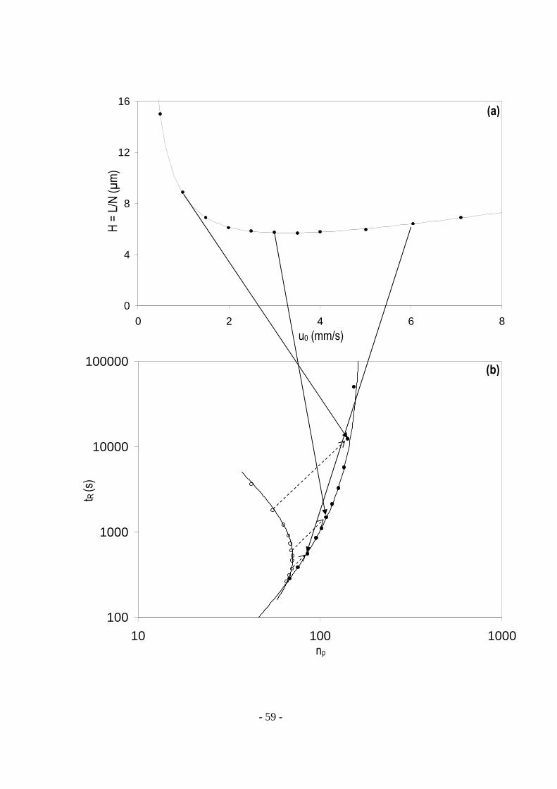
- 59 -

100

1000

10000

100000

10 100 1000

H = L/N (µm)

u0 (mm/s)

np

t R (s)

(a)

(b)

0

4

8

12

16

0 2 4 6 8

(a)

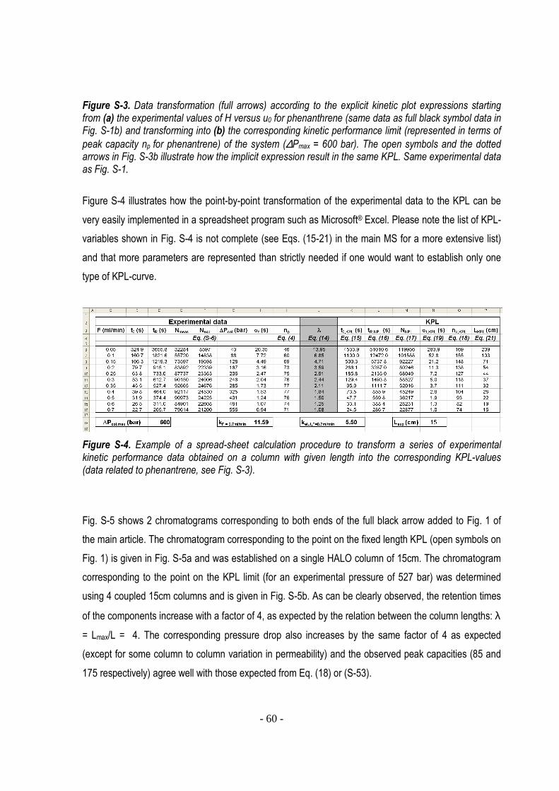
- 60 -

Figure S-3. Data transformation (full arrows) according to the explicit kinetic plot expressions starting from (a) the experimental values of H versus u0 for phenanthrene (same data as full black symbol data in Fig. S-1b) and transforming into (b) the corresponding kinetic performance limit (represented in terms of

peak capacity np for phenantrene) of the system (∆Pmax = 600 bar). The open symbols and the dotted arrows in Fig. S-3b illustrate how the implicit expression result in the same KPL. Same experimental data as Fig. S-1.

Figure S-4 illustrates how the point-by-point transformation of the experimental data to the KPL can be

very easily implemented in a spreadsheet program such as Microsoft® Excel. Please note the list of KPL-

variables shown in Fig. S-4 is not complete (see Eqs. (15-21) in the main MS for a more extensive list)

and that more parameters are represented than strictly needed if one would want to establish only one

type of KPL-curve.

Figure S-4. Example of a spread-sheet calculation procedure to transform a series of experimental kinetic performance data obtained on a column with given length into the corresponding KPL-values (data related to phenantrene, see Fig. S-3).

Fig. S-5 shows 2 chromatograms corresponding to both ends of the full black arrow added to Fig. 1 of

the main article. The chromatogram corresponding to the point on the fixed length KPL (open symbols on

Fig. 1) is given in Fig. S-5a and was established on a single HALO column of 15cm. The chromatogram

corresponding to the point on the KPL limit (for an experimental pressure of 527 bar) was determined

using 4 coupled 15cm columns and is given in Fig. S-5b. As can be clearly observed, the retention times

of the components increase with a factor of 4, as expected by the relation between the column lengths: λ

= Lmax/L = 4. The corresponding pressure drop also increases by the same factor of 4 as expected

(except for some column to column variation in permeability) and the observed peak capacities (85 and

175 respectively) agree well with those expected from Eq. (18) or (S-53).

- 61 -

The overlaid gray chromatogram on Fig. S-5b (see peaks denoted with *) illustrates the effect of an

inappropriate adjustment of the dwell time in gradient elution. By not inducing an additional delay time at

the start of elution, the mobile phase gradient reaches the front of the column earlier and as a result, the

elution window is decreased.

- 62 -

Figure S-5. Chromatograms corresponding to the 2 ends of the full arrow on Fig. 1 in the main article (see caption Fig. 1 for experimental conditions, F = 0.15 ml/min): (a) single HALO column (15cm), (b) 4

coupled HALO column (60cm) with appropriate adjustment of both β⋅t0 and tdelay/t0 (black) and with the

adjustment of β⋅t0 only, i.e. without correction on tdelay (gray, peaks denoted by an *).

20.3 min.

1.77 min.

12.6 min.

6.74 min.

∆∆∆∆Pcol = 127.5 bar np = 85

6.01 min.

∆∆∆∆Pcol = 527 bar np = 175

81.3 min.

50.1 min.

26.6 min.

*

*

*

(b)

(a)

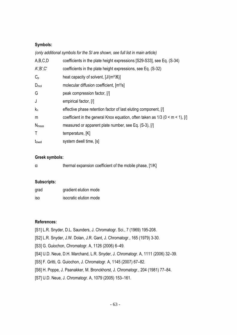
- 63 -

Symbols:

(only additional symbols for the SI are shown, see full list in main article)

A,B,C,D coefficients in the plate height expressions [S29-S33], see Eq. (S-34)

A',B',C' coefficients in the plate height expressions, see Eq. (S-32)

Cp heat capacity of solvent, [J/(m³⋅K)]

Dmol molecular diffusion coefficient, [m²/s]

G peak compression factor, [/]

J empirical factor, [/]

kn effective phase retention factor of last eluting component, [/]

m coefficient in the general Knox equation, often taken as 1/3 (0 < m < 1), [/]

Nmeas measured or apparent plate number, see Eq. (S-3), [/]

T temperature, [K]

tdwell system dwell time, [s]

Greek symbols:

α thermal expansion coefficient of the mobile phase, [1/K]

Subscripts:

grad gradient elution mode

iso isocratic elution mode

References:

[S1] L.R. Snyder, D.L. Saunders, J. Chromatogr. Sci., 7 (1969) 195-208.

[S2] L.R. Snyder, J.W. Dolan, J.R. Gant, J. Chromatogr., 165 (1979) 3-30.

[S3] G. Guiochon, Chromatogr. A, 1126 (2006) 6–49.

[S4] U.D. Neue, D.H. Marchand, L.R. Snyder, J. Chromatogr. A, 1111 (2006) 32–39.

[S5] F. Gritti, G. Guiochon, J. Chromatogr. A, 1145 (2007) 67–82.

[S6] H. Poppe, J. Paanakker, M. Bronckhorst, J. Chromatogr., 204 (1981) 77–84.

[S7] U.D. Neue, J. Chromatogr. A, 1079 (2005) 153–161.

- 64 -

[S8] P.J. Schoenmakers, H.A.H. Billiet, R. Tussen, L. De Galan, J. Chromatogr. A, 149 (1978) 519-

537.

[S9] F. Gritti, G. Guiochon, J. Chromatogr. A, 1212 (2008) 35–40.

[S10] F. Gritti, G. Guiochon, J. Chromatogr. A, 1178 (2008) 79–91.

[S11] U.D. Neue HPLC-Columns—Theory, Technology, and Practice; Wiley-VCH: Weinheim,

1997.

[S12] D. Cabooter, F. Lestremau, A. de Villiers, K. Broeckhoven, F. Lynen, P. Sandra, G. Desmet,

J. Chromatogr. A, 1216 (2009) 3895-3903.

[S13] Y. Zhang, X. Wang, P. Mukherjee, P. Petersson, J. Chromatogr. A, 1216 (2009) 4597–4605.

[S14] X. Wang, D.R. Stoll, A.P. Schellinger, P.W. Carr, Anal. Chem., 78 (2006) 3406-3416.

[S15] U.D. Neue, J. Chromatogr. A 1184 (2008) 107–130.

[S16] J.D. Stuart, D.D. Lisi, L.R. Snyder, J. Chromatogr. 1989, 485, 657-612.

[S17] M.A. Stadalius, H.S Gold, L.R. Snyder, J. Chromatogr., 327 (1985) 2745.

[S18] G. Desmet, D. Clicq, P. Gzil, Anal. Chem., 77 (2005) 4058-4070.

[S19] F. Gritti, G. Guiochon, Anal. Chem. 78 (2006) 5329-5347.

[S20] U.D. Neue, M. Kele, J. Chromatogr. A, 1149 (2007) 236-244.

[S21] S. Heinisch,J.-L. Rocca, G. Desmet, J. Chromatogr. A, 1203 (2008) 124-136.

[S22] M. Martin, G. Guiochon, J. Chromatogr. A, 1090 (2005) 16–38.

[S23] G. Desmet, J. Chromatogr. A, 1116 (2006) 1116, 89–96.

[S24] A. de Villiers, H. Lauer, R. Szucs, S. Goodall, P. Sandra, J. Chromatogr. A, 1113 (2009) 84-91.

[S25] F. Gritti, G. Guiochon, J. Chromatogr. A, 1166 (2007) 47-60.

[S26] K. Broeckhoven, G. Desmet, J. Chromatogr. A, 1216 (2009) 1325–1337.

[S27] J.R. Mazzeo, U.D. Neue, M. Kele, R.S. Plumb, Anal. Chem., 77 (2005) 460A-467A.

[S28] U. D. Neue, Y.-F. Cheng, Z. Lu, "Fast Gradient Separations", in "HPLC Made to Measure: A

Practical Handbook for Optimization", Stavros Kromidas, Ed., Wiley-VCH, Weinheim, 2006, pp. 47-58.

[S29] G. Desmet, K. Broeckhoven, Anal. Chem., 80 (2008) 8076–8088.

[S30] J.C. Giddings, Dynamics of Chromatography Part 1, Marcel Dekker: New York, 1965.

[S31] G. Guiochon, S. Golshan-Shirazi, A.M. Katti, Fundamentals of Preparative and Nonlinear

Chromatography, Academic Press: Boston, 1994.

[S32] A. Berdichevsky, U.D. Neue, J. Chromatogr. 535 (1990) 189.

- 65 -

[S33] G. Desmet, K. Broeckhoven, J. De Smet, G.V. Baron, P. Gzil, J. Chromatogr. A, 1188 (2008) 71-

188.