THE INTERACTION BETWEEN INTERNAL CONTROLASSESSMENT AND SUBSTANTIVE TESTING IN AUDITS

FOR FRAUD

Reed Smith

Sam Tiras

Stan Vichitlekarn

University of Oregon

Draft: October, 1997

Helpful comments were provided by Neil Fargher, Ray King, Steve Matsunaga, DaleMorse, Terry O’Keefe, Evelyn Patterson, and workshop participants at the University ofOregon.

THE INTERACTION BETWEEN INTERNAL CONTROLASSESSMENT AND SUBSTANTIVE TESTING IN AUDITS

FOR FRAUD

Abstract

We examine, from the auditor’s perspective, the interaction between internal control

evaluations and substantive testing in a model of fraud detection. The purpose of our study

is to examine a two-stage model of the auditor/manager interaction in which the auditor

assesses the “likelihood” or possibility of fraud in the first stage and conducts substantive

tests in a second stage. We compare this two-stage model to a model in which the auditor

is restricted to substantive testing only, in order to assess the incremental costs and benefits

of performing internal control evaluations. We find that the two models yield the same

equilibrium probability of fraud detection, but that the two-stage model achieves this level

of detection at a lower cost to the auditor.

- 1 -

THE INTERACTION BETWEEN INTERNAL CONTROLASSESSMENT AND SUBSTANTIVE TESTING IN AUDITS FOR FRAUD

1 Introduction

The Auditing Standards Board of the AICPA has recently issued Statement on

Auditing Standards (SAS) 82, which was intended to clarify the external auditor’s

responsibility for the detection of fraud in financial statements and to provide guidance to

CPAs in this endeavor. At the same time, Senator Ron Wyden introduced the Private

Securities Litigation Reform Act of 1995, which requires that external auditors attempt to

detect illegal acts that would affect the financial statements. These two developments

indicate a growing trend towards increasing the auditor’s responsibility for detecting fraud.

This heightened responsibility for fraud detection amplifies the importance of the

auditor’s evaluation of the system of internal control in the early stages of an audit. The

quality of the internal control system not only indicates exposures to particular frauds, but

also provides insight into management’s overall attitude towards protection against

fraudulent activity.

We examine, from the auditor’s perspective, the interaction between internal control

evaluations and substantive testing in a model of fraud detection.1 In particular, we analyze

a game-theoretic interaction between an external auditor and management of the client firm

in a model in which the strength of controls is related to the propensity of the manager to

commit fraud. In addition, the (dishonest) manager chooses whether or not to commit

fraud. The auditor chooses the amount of audit work to perform in the assessment of

internal control and, depending upon the results of this assessment, the amount of

substantive testing to perform in an attempt to discover fraud.

1 This paper defines fraud in a manner consistent with Statement on Auditing Standards (SAS) number 82.Fraud is an intentional employee action which benefits the employee but is detrimental to the firm. Fraud,in our context, could be defalcation covered up by misreporting or simply misreporting for its own sake.We do not, however, consider report conditional auditing as in Newman, Rhoades, and Smith [1996].

- 2 -

The purpose of our study is to introduce a two-stage model of the auditor/manager

interaction in which the auditor exerts costly effort in an attempt to assess the “likelihood”

or possibility of fraud in the first stage and conducts substantive tests in a second stage.

We compare this two-stage model to a benchmark model in which the auditor is restricted

to substantive testing only, in order to assess how the equilibrium strategies and outcomes

are affected by the availability of costly internal control evaluation. In addition, we provide

some descriptive predictions about how various characteristics in the audit environment

affect the allocation of audit work across the two stages and how these characteristics affect

the manager’s fraud decision.

We find that the likelihood that fraud is perpetrated and the ex ante likelihood that it

is detected in equilibrium is not affected by whether or not internal control evaluations are

performed. However, we find that when these evaluations are performed, the equilibrium

cost of auditing is lower. This cost savings diminishes, however, as the ex ante

probability of a fraud-prone manager increases. In particular, as this probability increases,

(equilibrium) system assessment effort in the first-stage of the audit decreases because

substantive testing converges to the level of substantive testing in the benchmark game. In

other words, substantive testing will not be as responsive to the results of internal control

evaluations.

In addition , we find that as the effectiveness of substantive testing procedures

increases, the relative benefits of system assessment decrease and substantive testing again

converges to the level of substantive testing in the benchmark game. Audit firms that have

invested in an audit technology that increases the effectiveness of substantive testing are

expected to rely more heavily on substantive testing than on internal control reviews. The

potential cost savings to these firms from shifting audit resources to system evaluations are

minimal or non-existent. This result casts doubt on whether SAS 82 achieves the purpose

of increasing audit effectiveness by forcing these types of firms to allocate more audit

resources to system evaluation. We find that the probability of undetected fraud is not

- 3 -

affected by whether the auditor allocates resources to system evaluation. Only the audit

costs are affected.

Much of the previous literature in strategic auditing has focused on situations in

which the auditor makes a single decision. Newman and Noel [1989] and Shibano [1990]

both focus on the auditor’s accept/reject decision given a fixed sample of audit data.

Patterson [1993] extends these studies by considering the auditor’s accept/reject decision

after a sample size decision. Our model differs from these studies in two fundamental

ways. First, we model the audit as a discovery problem, where these papers model an

acceptance audit. Second, examine a two-stage audit interaction in which the auditor makes

effort decisions at the different stages.

This paper can be viewed as a first attempt at modeling the two-stage audit detection

problem addressed by SAS 82 in which the first stage involves system evaluation and the

second stage involves fraud detection. Few papers in strategic auditing have examined

allocations of audit work across time. Three papers which have addressed these issues are:

Caplan [1997], Park [1994], and Finn and Penno [1996]. Caplan [1997] examines a

multi-stage audit setting in which the manager has a two-stage decision, but the audit work

is essentially a one-stage problem. Park [1994] examines an audit allocation problem in

which the manager decides how much to steal in each of two periods and the auditor

decides how much auditing to perform in each of the two periods. Finn and Penno [1996]

examine the issue of commitment in a stop-and-go audit environment. Their paper focuses

on when to stop auditing, if no fraud has been discovered.

Our paper complements the Caplan [1997] paper in that we examine a two-stage

audit in which the first stage is system related. In other words, unlike Finn and Penno

[1996] and Park [1994], detection of fraud cannot occur in the first stage. Caplan’s [1997]

focus is on the manager’s first-stage decision (system choice), while we simplify that

choice and focus on the auditor’s first-stage decision (system evaluation).

- 4 -

The remainder of this paper is organized as follows: In section 2 we present and

discuss the simple benchmark model; in section 3, we present the details of our two-stage

model, in section 4 we describe our analysis, and in section 5 we discuss our results and

identify limitations of our study.

2 Benchmark model

As a benchmark, we begin with a restricted interaction between a manager, who

may wish to perpetrate a fraud, and an auditor who wishes to detect fraud. Managers are

of two types, dishonest managers, which arise with probability θ ; and honest managers,

which arise with probability 1 −θ( ) . Honest and dishonest managers are defined according

to their reward from successfully (i.e. without detection) perpetrating a fraud. Honest

managers obtain no benefit for fraud; whereas dishonest managers obtain a benefit of F.

In the benchmark model, the auditor cannot assess whether the manager is honest

or dishonest, and will choose a level of substantive testing (audit effort), denoted e > 0

based upon his knowledge of θ .2 If the manager chooses to commit fraud, the auditor will

detect the fraud with probability, d[e]. We assume that d[e] has the property:

d' e[ ] = τ 1 − d e[ ]( ) where τ > 0 is an audit effectiveness parameter. The effectiveness of

the audit increases with increases with τ.3, 4 The manager of type t ∈ g,b{ } will commit

fraud (as a mixed strategy) with probability αt ∈ 0,1[ ] .

2 In the next section, we will add a strategy in which the auditor can exert effort e

c to possibly learn

whether the manager is honest or dishonest.3 This property is consistent with sampling under both the Poisson (see Newman, Park, and Smith [1997])and the Binomial distributions. In addition, sampling under the Hypergeometric distribution also satisfiesthe condition approximately (in the case of the Hypergeometric, τ is also a function of e). Note that thiscondition has implications for higher order derivatives as well. For example:

d" e[ ] = τ 1− d e[ ]( ) −d' e[ ]( ) = −τ 21 − d e[ ]( ) .

4 τ can be thought of as an inverse to the unit cost of auditing. For example, if detection were given by:d x[ ] = 1− Exp −x{ }( ) , and each unit of effort costs τ , we could define e = 1 τ( )x and rewrite the

detection probability in terms of e: d e[ ] = 1 − Exp −τ e{ }( ) where each unit costs 1 and the total cost is e.

Note that for this detection probability: d' e[ ] = τ Exp −τ e{ } = τ 1 − d e[ ]( ) .

- 5 -

The benefit to the dishonest manager of committing fraud and getting away with it

(not being detected) is F. The honest manager has a benefit of 0 for this outcome. The

penalty to both type of managers for detected fraud is PD . As a result, honest managers (as

a weakly dominant strategy) will never choose to commit fraud.

The auditor incurs audit costs of e to determine whether fraud has been committed.5

If the auditor fails to detect existing fraud, he suffers a penalty, D, which would include

legal damages, reputation loss, and governmental sanctions. This cost is avoided if the

auditor detects fraud. These payoffs are shown in the game tree below:

***************************Insert Figure 1 about here

***************************

The solution to this game is straight forward. The manager’s choice of αb* must

make the auditor’s equilibrium choice of e* optimizing and the auditor’s choice of e* must

make the manager’s choice of αb* optimizing. The auditor’s expected payoff is computed

as:

−θ αbD 1 − d e[ ]( )− e . (1)

The first-order condition for this payoff is:

−1 + θ αb Dτ 1 − d e[ ]( ) = 0 , (2)

and the second-order condition is:

−θα b Dτ2 1− d e[ ]( ) < 0. (3)

The dishonest manager’s payoff is:

αb F 1 − d e[ ]( ) − PD d e[ ]( ). (4)

Since the manager has mixed-strategy over a binary choice, the following condition must

hold in any completely mixed-strategy:

5 Without loss of generality, the unit cost of auditing is normalized to 1.

- 6 -

F 1 − d e[ ]( ) = PD d e[ ]. (5)

We characterize the equilibrium strategies to the benchmark game in proposition 1.

Proposition 1. The dishonest manager, in equilibrium, will commit fraud with

probability, 6

αb* =

F + PD

DτθPD

. (6)

The auditor, in equilibrium, will choose e such that:

d e*[ ] =F

F + PD . (7)

The proof follows directly from (2) and (5).

Comparative static analysis shows many similarities between this equilibrium and

the equilibria in Newman and Noel [1989] and Shibano [1990]. Before we describe our

comparative statics, however, we will compute the ex ante probability of undetected

fraud (UF): pr UF[ ] =θα b* 1− d e*[ ]( ) =

PD F + PD( )θDτθPD F + PD( ) =

1

Dτ.

Using direct partial differentiation of (6) and (7), we obtain the following

comparative statics in Table 1.

6 In addition, it is necessary that F + P

D≤ P

DτθD so that αb

* <1 . If this inequality does not hold, then

Proposition 1 does not describe equilibrium. This possibility is considered in section 4.5.

- 7 -

∂∂D

∂∂F

∂∂PD

∂∂τ

(7)∂

∂θ

Probability a dishonest managerwill commit fraud, αb

* - + - - -

Newman and Noel and Shibano - + - NA NA

Patterson - + - - NA

Probability a fraud will be detected,d e*[ ]

0 + - 0 0

Newman and Noel and Shibano 0 + - NA NA

Patterson + + - + NA

Probability of undetected fraud,pr UF[ ]

- 0 0 - 0

Newman and Noel and Shibano - +/- +/- NA NA

Patterson - +/- +/- +/- NA

Table 18

Comparative statics in the benchmark game(with comparisons to literature)

The comparative statics from our study (for the auditor’s strategy, d e*[ ] and the

manager’s fraud strategy, αb* ) are similar to the results of Newman and Noel [1989] and

Shibano [1990] (to the extent that the problems can be compared), even though we look at

a different type of audit decision. On the other hand, Patterson [1993] finds that detection

7 To compare τ between our study and Patterson, we interpret τ as an inverse of unit cost of auditing.

- 8 -

risk is increasing in (what we refer to as) D. The difference between our study and the

Patterson study results from our focus on fraud discovery and her focus on acceptance

auditing. We do not consider type I errors and, as a result, increased effort always serves

to improve the auditor’s expected reporting decision. Patterson does consider the costs of

type I errors and the auditor, in her model, balances the costs of type I and type II reporting

errors in choosing the optimal effort and cutoff values.

An interesting result of our model relates to the equilibrium probability of

undetected fraud. In our model, this probability is 1

Dτ which depends only on D and τ .

The equilibrium probability of detecting a fraud if it occurs (the auditor’s strategy) in (7)

and the equilibrium probability that a fraud occurs (θ times the manager’s strategy) in (6)

partially cancel so that the resulting probability that fraud is undetected is a constant. The

nature of the payoffs in the each of the other three studies does not allow them to specify a

closed form for the probability of undetected error. But their comparative statics are

consistent with ours in that the probability of undetected fraud is decreasing in the auditor’s

expected costs for undetected fraud and may be increasing or decreasing in the manager’s

gross payoff for undetected fraud (which we refer to as F). We find that this comparative

static is 0, which is (of course) neither increasing or decreasing.

We now extend our benchmark model by allowing the auditor to allocate effort in a

first stage to (possibly) discover the manager’s propensity to commit fraud.

3 Two-stage model

We extend the benchmark interaction in section 2 to a two-stage interaction by

adding a strategy for the auditor. The auditor can assess the likelihood that the manager is

dishonest by exerting effort in a first stage. As a result of this effort, the auditor either

learns that the manager is dishonest (and prone to fraud) or learns nothing (a null signal).

8 The letters NA in a cell imply that a comparison cannot be made between the papers because the otherauthors did not examine this comparative static.

- 9 -

We describe the sequence of events in the two-stage model in section 3.1. The payoffs to

the auditor and manager are derived in section 3.2, and the equilibrium concept is defined

in section 3.3.

3.1 Sequence of events

In the first stage of our model, the manager’s type is determined (honest (g) or

dishonest (b)). The dishonest manager is assumed to always have a weak system in order

to allow fraud to be perpetrated;9 the honest manager always chooses a strong system.10

The auditor attempts to determine whether the system of internal control is strong or weak

by exerting effort, e c > 0. We assume that the probability that the auditor will mistakenly

identify a strong system of internal control as weak is zero and the probability that the

auditor will identify a weak system of internal control as being weak is h e c[ ]. h e c[ ] is

assumed increasing-concave over the range [0,1), and h[0]=0.

Based upon his observations in the first stage of the model, the auditor will choose

a level of substantive testing (audit effort) in the second stage. The auditor’s choice, if he

does not find weaknesses in the control system, will be denoted e0> 0; his choice, if he

does observe weaknesses in the control system, will be denoted ew > 0. As in the

9 This assumption regarding the incentives of dishonest managers to choose weak systems of controlappears consistent with some notable audit failures. In particular, the control systems at PharMor and ZZZBest were notoriously poor and allowed management free hand in committing fraud. We admit, however,that there are several alternative choices for modeling at this point. For example, we could allow manager achoice of system quality. In this case, dishonest managers would be attempting to fool auditors intobelieving that they are honest by choosing “high quality” systems. Such a choice would necessarily makefraud more difficult or more costly. Since we are focusing on the structure of the auditor’s problem, wesimplify the problem by assuming that the auditor learns the manager’s “propensity” for fraud if a weaksystem is discovered. Caplan [1997] provides an interesting alternative to this model in which the audit isstrategically fixed (stochastic) and the manager’s system choice is a focus of the model.10 There are many reasons that honest managers would prefer strong systems. In particular, honestmanagers might believe that long-run cost savings can be obtained by choosing strong systems. Anotherreason that honest managers (at any given level of the organization) would be inclined to choose strongsystems is that it would also reduce the risk of fraud or delfalcation committed by their subordinates, butwhich they might be held accountable for.

- 10 -

benchmark model, if the manager chooses to commit fraud, the auditor will detect the fraud

with probability, d e[ ], where e is either e0 or ew .11

The dishonest manager knows that the auditor will identify him as dishonest with

probability h e c[ ].12 We will denote the (mixed-strategy) probability that the manager

commits fraud as αt ∈ 0,1[ ] , where t ∈ g,b{ } is the manager’s type. The sequence of

events is depicted in the timeline below:

***************************Insert Figure 2 about here

***************************

3.2 Payoffs

The payoffs to the honest and dishonest managers are identical to those in the

benchmark game. Dishonest managers obtain a benefit of F for undetected fraud; honest

managers obtain a benefit of 0 for undetected fraud; and both manager types incur a cost

(penalty) of PD if they are detected committing fraud.

The auditor incurs audit costs of e c in attempting to determine if the internal control

system is weak. If the system is found to be weak, the auditor then incurs audit costs of

ew to determine whether fraud has been committed. If the system is not found to be weak,

the auditor incurs audit costs of e0 to determine whether fraud has been committed. The

existence of a strong or weak system does not affect the probability, d[e], of detecting

fraud. Again, if the auditor fails to detect existing fraud, he suffers a penalty, D, which is

avoided if the auditor detects fraud. These payoffs are shown in the game tree below:

***************************Insert Figure 3 about here

***************************

11 We assume that d[e] is identical to the detection probability in the benchmark game and has all of thesame characteristics.12 The model of detection in this paper (for internal control and fraud detection) assumes that the auditorcannot find evidence of a “weak” system when it is strong or evidence of “fraud” when no fraud exists.

- 11 -

3.3 Nature of equilibrium

Equilibrium will be a 4-tuple of strategies: αb ,e c,e w ,e 0{ }.13 These strategies are

identified below:

αb : The (mixed-strategy) probability that the dishonest type of manager will commitfraud.

e c : The effort that the auditor supplies to determining whether the firm has a strong orweak system of internal controls.

ew : The effort that the auditor supplies to detecting fraud if he has found that the firmhas a weak system of internal controls.

e0 : The effort that the auditor supplies to detecting fraud if he has not found that thefirm has a weak system of internal controls. Note that this does not imply that hehas concluded that the controls are strong.

Equilibrium requires that each of these strategies be played in accordance with

Bayes’ Rule and that each strategy be a Nash best-reply to the other player’s strategy. In

addition, we require that all choices be sequentially rational.

4 Analysis of the two-stage model

In this section, we characterize the equilibria to our two-stage model, describe how

these equilibria are affected by changes in the parameters, and compare these equilibria to

those of the benchmark game. In section 4.1, we describe the payoff functions of the

auditor and dishonest manager, and describe the first-order conditions for the game. In

section 4.2, we characterize the equilibrium strategies to the game and in section 4.3, we

examine the interactions between parameters and equilibrium choices (comparative statics).

We compare this model to the benchmark model in section 4.4. We examine the

robustness of our equilibrium in section 4.5 and provide a numerical example in section

4.6.

13 We will ignore the strategy of the honest manager since committing fraud is weakly dominated.

- 12 -

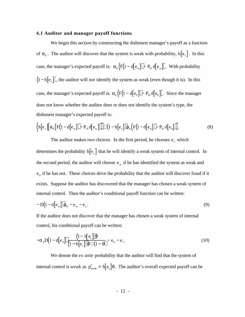
4.1 Auditor and manager payoff functions

We begin this section by constructing the dishonest manager’s payoff as a function

of αb . The auditor will discover that the system is weak with probability, h e c[ ]. In this

case, the manager’s expected payoff is: αb F 1 − d ew[ ]( ) − PD d ew[ ]( ) . With probability

1 − h e c[ ]( ) , the auditor will not identify the system as weak (even though it is). In this

case, the manager’s expected payoff is: αb F 1 − d e0[ ]( ) − PD d e0[ ]( ) . Since the manager

does not know whether the auditor does or does not identify the system’s type, the

dishonest manager’s expected payoff is:

h e c[ ] αb F 1 − d ew[ ]( ) − PD d ew[ ]( )( ) + 1 − h e c[ ]( )αb F 1 − d e0[ ]( ) − PD d e0[ ]( )( ) . (8)

The auditor makes two choices. In the first period, he chooses e c which

determines the probability h e c[ ] that he will identify a weak system of internal control. In

the second period, the auditor will choose ew if he has identified the system as weak and

e0 if he has not. These choices drive the probability that the auditor will discover fraud if it

exists. Suppose the auditor has discovered that the manager has chosen a weak system of

internal control. Then the auditor’s conditional payoff function can be written:

− D 1 − d ew[ ]( )αb − ew − e c . (9)

If the auditor does not discover that the manager has chosen a weak system of internal

control, his conditional payoff can be written:

−α bD 1 − d e0[ ]( ) 1− h ec[ ]( )θ1 − h e c[ ]( )θ+ 1 − θ( ) − e0 − e c. (10)

We denote the ex ante probability that the auditor will find that the system of

internal control is weak as pweake = h ec[ ]θ. The auditor’s overall expected payoff can be

- 13 -

computed as pweake multiplied by the expression in (9) and (1- pweak

e ) multiplied by the

expression in (10):

−e c − h e c[ ]θ D 1 − d ew[ ]( )α b + ew( ) − 1− h e c[ ]θ( ) e0 +1 − h e c[ ]( )θD1 − d e0[ ]( )

1− h e c[ ]( )θ+ 1−θ( )

. (11)

The auditor’s payoff in (11) can be simplified:

−e c − ew θ h ec[ ] − e0 1−θ h e c[ ]( ) −θαb D h e c[ ] 1 − d ew[ ]( ) + 1− h ec[ ]( ) 1 − d e0[ ]( )( ). (12)

Using the payoffs in (8) and (12), we can describe first-order conditions for the

game. The dishonest manager’s choice is the probability of fraud, αb . The auditor

chooses his first stage effort, e c ; his effort if he learns that the control system is weak, ew ;

and his effort if he does not learn that the control system is weak (it may not be), e0 .

The manager’s first-order condition is:

F − F + PD( ) d e0[ ] 1− h e c[ ]( ) + d ew[ ]h e c[ ]( ) = 0 . (13)

If the auditor observes that the system of controls is weak (with probability θ h ec[ ] ), his

payoff is:

−e c* − ew − Dαb 1− d ew[ ]( ) , (14)

where e c* is a constant (at this point in the game). This yields the following first-order

condition:

1 − Dαbd' ew[ ] = 1− Dα bτ 1 − d ew[ ]( ) = 0 . (15)

The second-order condition for the auditor (in this information set) is:

−Dαbτ 1 − d ew[ ]( ) < 0. (16)

As a result, if the auditor finds himself in this information set, the choice of ew which

satisfies the first-order condition in (15) will be an optimum.

If the auditor does not observe that the system of controls is weak (which occurs

with probability 1 −θ h e c[ ]( )), his payoff is:

- 14 -

−Dθ 1− d e0[ ]( ) 1 − h ec

*[ ]( )αb

1 − h e c*[ ]θ − e c

* − e0 .14 (17)

The auditor’s first-order condition (in this information set) is:15

Dθ 1 −d e0[ ]( )τ 1− h ec*[ ]( )αb − 1− h ec

*[ ]θ( ) = 0 . (18)

The second-order condition for the auditor (in this information set) is:

−Dθτ2 1 − d e0[ ]( ) 1− h ec[ ]( )α b

1− θh e c[ ]( ) < 0 . (19)

Similar to the case in which the auditor observes that the system of controls is weak, if the

auditor finds himself in this information set in which he does not observe that the controls

are weak, his choice of e0 which satisfies the first-order condition in (18) will be an

optimum.

4.2 Equilibrium strategies

In this section, we characterize the equilibrium strategies of the manager (αb* ) and

the auditor (e c* , ew

* , and e0* ). Proposition 2 describes the strategies of the players in the

second-stage of the game. Proposition 3 characterizes the auditor’s choice of e c* in the first

stage of the game.

Combining (13), (15), and (18), we can obtain characterizations of αb* , e0

* , and ew*

as functions of e c* . These characterizations are described in Proposition 2.

Proposition 2. The dishonest manager, in equilibrium, will commit fraud with

probability,

αb* =

F + PD

DτθPD

(the same as in the benchmark model). 16 (20)

14 Again, the auditor would have already committed resources of e

c

* to the first-stage of the audit at this

point.15 Note we are using the assumption that: d' e[ ] = τ 1 − d e[ ]( ) here.16 Again, it is necessary that F + P

D≤ P

DτθD so that α

b

* < 1.

- 15 -

The auditor, in equilibrium, will choose ew to satisfy:

d ew*[ ] =

F + PD 1 −θ( )F + PD

, (21)

and e0 to satisfy:

d e0*[ ] =

F − h e c*[ ] F + PD 1 −θ( )( )

1 − h ec*[ ]( ) F + PD( )

. (22)

The proof follows immediately from the first-order conditions in (13), (15), and (18) given

that the second-order conditions in (16) and (19) are satisfied for all parameter choices.

In this model, the strategy of the dishonest manager is driven by the auditor’s

conditional payoff in the information set in which he observes weak controls. In other

words, αb must satisfy the auditor’s first-order condition in (15). This yields a value:

αb = Dτ 1− d ew[ ]( )( )− 1

. For the auditor’s equilibrium choice of d ew*[ ] , the manager will

choose αb to satisfy the auditor’s first-order condition in (15). To find the auditor’s

choices of e c* , ew

* , and e0* , we must substitute (15) into (13) and (18) and solve

simultaneously for d ew[ ] and d e0[ ] . We will then substitute back the value of d ew*[ ] in

(21) into αb = Dτ 1− d ew[ ]( )( )− 1

to obtain the value of αb* in (20).

Notice that the expression for d ew[ ] in (21) does not depend upon h e c[ ], but that

the expression for d e0[ ] in (22) does. This is because if the auditor has observed weak

controls, he knows that the manager is dishonest and has a desire to commit fraud. As a

result, he conditions his effort only on the equilibrium probability that the dishonest

manager will commit fraud.

As an immediate corollary of Proposition 2, we can compare the equilibrium

magnitudes of audit (detection) effort in the two information sets. This result is described

in Corollary 1.

- 16 -

Corollary 1. Equilibrium audit effort in the information set in which the auditor has

observed that the system of controls is weak (ew* ) is always greater than the equilibrium

audit effort in the information set in which the auditor has not observed weak controls.

The proof is obtained by comparing the magnitudes of (21) and (22).

The next segment of our analysis will focus on the characterization of audit effort in

the first stage of the game, e c . The manager’s strategy (whether honest or dishonest) is

completely characterized as is the auditor’s strategy in the second stage of the game. We

now incorporate these choices into the auditor’s first-stage problem. The auditor’s

expected payoff in the first stage is given by (12). Taking the first-order condition of this

expected payoff with respect to the first-stage choice of e c , we obtain:

−1 + θh' e c[ ] e0 − ew + Dαb d ew[ ] − d e0[ ]( )( ) = 0 . (23)

Using our equilibrium conditions from proposition 2, we can obtain a characterization of

h' e c*[ ] in terms of h e c

*[ ] , e0* , ew

* , and the parameters. This characterization is described in

proposition 3.

Proposition 3. Suppose that (23) induces a feasible choice of e c* for which

h e c*[ ] ∈ 0,1( ) and:17

h'' ec*[ ] ≤ −

1 −θ( )2 τ2 1 − h e c*[ ]( )

1−θh e c*[ ]( ) 1 −θ 1− τ 1 − h e c

*[ ]( ) e0* − ew

*( )( )( )3 . (24)

Then, the auditor’s equilibrium strategy in the first stage of the game is given by:

h' e c*[ ] =

τ 1 − h e c*[ ]( )

1 −θ 1 −τ 1 − h e c*[ ]( ) e0

* − ew*( )( ) . (25)

(proof in appendix)

17 A feasible solution to (16) is a solution to the equation for which e

c

* is a feasible value. Since e

c

*

depends upon ew

* and e

0

*, it is possible that no such solution exists.

- 17 -

Notice that h' e c*[ ] in (25) is a function of e0

* . Recall also that the auditor’s

equilibrium choice of e0 in (22) was a function of h e c[ ]. This co-dependence of e c* and

e0* , combined with a detection technology in which d' e[ ] = τ 1− d e[ ]( ) , will make closed-

form solutions impossible, even if we specified a detection probability. This fact will be

obvious in section 4.6 where we employ numerical techniques to solve a parameterized

example. The problem is not that a solution does not exist, though. The problem is that

the expression in (25) will be intractable in closed form. As a result, we will focus on

characterizing the solution as much as possible using comparative static analysis and

numerical analysis.

We now turn to our comparative static analysis of the game. Section 4.3 will

describe how changes in parameters (for interior equilibria) affect the equilibrium choices

of the dishonest manager and the auditor. Section 4.4 will compare the equilibria in the

benchmark game with those of the two stage game. We will discuss situations in which an

interior equilibrium does not exist in section 4.5.

4.3 Comparative Static Analysis

We now consider how changes in F, PD , D, τ, and θ affect the equilibrium

choices: e c* , e0

* , ew* , and αb

* , by applying the Implicit Function Theorem to the system of

first-order conditions identified in Proposition 2 and Corollary 1.18 Using this approach,

we obtain the comparative static results described in Table 2.19

18 For a detailed description of this approach, see Chiang [1989] pages 210 - 212.19 The proof of these results is in the appendix.

- 18 -

∂∂ D

∂∂ F

∂∂ PD

∂∂τ

20 ∂∂θ

Audit effort in system evaluation, e c*

0 0 0 — —

Probability of fraud detection when aweak system is observed, d ew

*[ ] 0 + — 0 —

Probability of detection when noweaknesses are observed, d e0

*[ ] 0 + — + +

Difference between e0* and ew

*

ew* − e0

*( )0 — + — —

Probability a dishonest manager willcommit fraud, αb

* — + — — —

Table 2Comparative statics for the two-stage game

20 The derivatives of e

w

* and e

0

* are the same as the derivatives of d e

w

*[ ] and d e0

*[ ], except for ∂ew

*/ ∂τ

and ∂e0

*/ ∂τ . We focus on the derivatives of the “detection probability” rather than “effort” in order to

demonstrate that the probabilities converge on d e*[ ] from the benchmark model. It is straight forward

that if ∂ d ew

*[ ] / ∂τ =0 (as shown in the table), then ∂ew

*/ ∂τ must be negative. What is not as clear is

that ∂e0

*/ ∂τ can be negative, too. This is because an increase in the effectiveness parameter (or,

equivalently, a decrease in the unit cost) allows “more” auditing to be done (in terms of probability) ata lower level of effort. This is illustrated in the numerical example of section 4.6.

The comparative statics for ew* and αb

* can be obtained directly from the equilibrium

conditions in (20) and (21). The comparative statics for e0* and e c

* require that we apply

the Implicit Function Theorem to the system of equations.

This analysis provides some noteworthy results. Consider the comparative statics

for ew* . The auditor’s effort in detecting fraud, given that he knows that he is dealing with

a dishonest manager is driven by the manager’s incentives for fraud (F and PD ) in the

intuitive direction. It is a bit surprising, though, that the auditor’s effort is a decreasing

function of the ex ante likelihood that the manager is dishonest. This is especially

- 19 -

surprising since the parameter, θ , does not appear in either of the first order conditions

(13) or (15). This implies that the influence of θ on ew* and αb

* must derive as a second-

order effect from the changes of θ on e0* and the effect of e0

* on ew* . Notice that θ does

appear in the first-order condition in (18) for the auditor if he has not observed any

weaknesses in internal control. And recalling the relationship between αb* and d ew

*[ ] , this

equation also contains an expression for d ew*[ ] . Hence (18) will cause d e0

*[ ] to be

responsive to changes in θ and will also, in turn, cause ew* and αb

* to respond to changes

in θ . The lack of responsiveness of ew* to changes in D and τ result primarily from the

fact that the manager’s first-order condition in (13) does not depend upon these parameters.

Unlike comparative statics for ew* and αb

* , which can be obtained directly from the

equilibrium expressions in (20) and (21), the comparative statics for e0* are a bit more

complicated. As an example, note that τ does not appear in the expression for d e0*[ ] in

(22). But, (from Table 2), dd e0

*[ ]d τ

> 0 . The impact of τ on d e0*[ ] must derive from the

impact of τ on e c* and the impact of e c

* on e0* . We derive these comparative statics by

applying Cramer’s rule and the Implicit Function Theorem. Consider dd e0

*[ ]d τ

as an

example. This derivative will be the third element of the vector product:

∂∂τ

∂A

∂e c

,∂A

∂e0

,∂M

∂α b

• J−1 where J is the matrix of second order partials.

∂∂τ

∂A

∂e c

,∂A

∂e0

,∂M

∂α b

• J−1 can be rewritten:

θ d ew*[ ]− d e0

*[ ]( )h' e c*[ ]

τ2 1 − d ew*[ ]( ) , 0, 0

, which implies

that we are only concerned with the first column of J−1 . So a single element of J−1 will

- 20 -

determine the sign of dd e0

*[ ]d τ

, but this element involves derivatives with respect to ew , e0 ,

αb , and e c . The details of the computation are given in the appendix. The surprising

result that increases in audit technology increase the auditor’s choice of detection

probability when a weak system is not detected is attributable to the fact that increases in τ

induce decreases in e c* which then cause d e0

*[ ] to increase. This result demonstrates our

argument that audits in which substantive testing procedures are effective will correspond

to a decreased focus on internal control evaluation, since d ew*[ ] and d e0

*[ ] will be

converging on the benchmark detection probability, d e*[ ] .

Finally, consider the difference between ew* and e0

* . Our comparative statics show

that this difference is decreasing in F,τ , and θ and is increasing in PD . The results for τ

and θ can be obtained simply by examining the comparative static results for ew* and e0

* .

And since ∂e c

*

∂F=

∂e c*

∂PD

= 0 , the results for F and PD can be obtained by computing d ew*[ ] -

d e0*[ ] using (21) and (22).21

The nextsection constrasts the solutions of section 4 to the solutions to the

benchmark game in section 2 to explicitly demonstrate the benefits from internal control

evaluations.

4.4 Comparison of the benchmark model and the two-stage model

In the benchmark model, the equilibrium audit effort required that the equilibrium

probability that a fraud would be detected, if it exists, is given by: d e*[ ] =F

F + PD

. In the

two-stage model, we can obtain an expression for the equilibrium that a fraud would be

detected by computing: h e c*[ ]d ew

*[ ]+ 1 − h e c*[ ]( )d e0

*[ ], where h e c*[ ] is characterized by

21 Since the derivatives of e

c

* are zero, only the direct effects are important in evaluating this difference.

- 21 -

(25), d ew*[ ] is characterized by (22) and d e0

*[ ] is characterized by (23). Computing this

value, we find that for the two-stage model, the probability of detecting a fraud if it exists

is still F

F + PD

. Hence, the equilibrium probability of detection is the same for both

models. In addition, we note that the manager’s fraud strategies in (6) and (20) are

identical. Note, however, that in the two-stage model, the auditor could trivially choose the

benchmark model by choosing e c =0 (which implies by assumption that h e c[ ] = 0). As a

result, we conclude that the two-stage model at least weakly dominates the benchmark

model, since the auditor would only choose e c* > 0 if it would decrease his ex ante

expected total costs. This result is important because it demonstrates that the potential

benefits to internal control assessment lie in audit cost decreases, not in more (ex ante)

effective audits.

We formalize this result in corollary 2.

Corollary 2: Suppose the conditions in proposition 2 are satisfied and that e c* > 0. The

ex ante cost of auditing using a two-stage audit, e c* +θ h ec

*[ ]ew* + 1 −θ h e c

*[ ]( )e0* is less

than the cost of auditing using a benchmark audit, e* .

Corollary 2 will be illustrated with our numerical example in section 4.6.

To understand better how the benchmark and two-stage models relate, we will

compare the equilibrium values of d e[ ], d ew[ ], and d e0[ ] . By observation, we see that

d ew*[ ] > d e*[ ] , but that the difference is decreasing in θ . Using a similar comparison, we

observe that d e*[ ] > d e0*[ ] and, since

∂e0*

∂θ> 0 , this difference is also decreasing in θ . As

a result we conclude d ew*[ ] > d e*[ ] > d e0

*[ ] and that d e*[ ] is a weighted average of d ew*[ ]

and d e0*[ ] (weighted by h e c

*[ ] and 1 − h e c*[ ]( ) respectively). As θ increases, d ew

*[ ] and

- 22 -

d e0*[ ] converge to d e*[ ] from above and below respectively. Also, as θ increases, the

value of e c* decreases. At some point the value of e c

* = 0 and the two models are identical.

Since we know that the equilibrium probability of detection is F

F + PD

for both the

benchmark and the two-stage games, we can compute the expected probability of

undetected theft. This is given by probability of a dishonest manager, θ , multiplied by the

probability that the dishonest manager will commit fraud (recall that it is the same under

both the one and two-stage games): αb =F + PD

D τθ PD

, multiplied by the probability of not

detecting the fraud: 1 −F

F + PD

=PD

F + PD

. Multiplying these values we obtain the

probability (ex ante) that an audit failure will occur, 1

D τ. Hence, the occurrence of audit

failures is decreasing in D (the auditor’s penalty) and in the effectiveness parameter, τ . It

is important to note, though that this decrease in audit failures does not result from

increased effort on the part of the auditor; rather it results from a decreased likelihood that

the dishonest manager will commit fraud.

Section 4.5 will address situations in which the solutions to (22), (23), and (25) are

infeasible.

4.5 Robustness

Since (25) characterizes e c* as a function of ew

* and e0* , and the functions h e c[ ] and

h' e c[ ] , it is quite possible that no feasible algebraic solution exists. While there does

always exist a solution to equation (25) over the domain of the real numbers, there is no

guarantee that the solution will yield a positive number.22 If the solution is not positive,

then the auditor will choose e c*=0; which implies that h=0. As noted above, this situation

22 This issue is much more likely to arise than a situation in which (17) does not hold. Note if (17) doesnot hold, then the solution is a minimum rather than a maximum - which is unlikely.

- 23 -

is identical to the situation in which the auditor cannot assess the likelihood of fraud by

evaluating the system of controls and must rely on substantive testing exclusively as

represented by our benchmark model.

Note also that if F + PD > D τθ PD , the equilibrium value of αb* is the boundary

value (1). If αb* =1, then the auditor’s problem becomes a straightforward optimization

problem over e c , ew , and e0 . In this case, the auditor’s strategy will depend only upon

the factors directly affecting his payoff: D, θ , and τ .

4.6 Numerical Example

In our numerical example, we will illustrate that the two-stage model yields the

same equilibrium probability of detection at a lower cost than does the benchmark model.

In addition, we will also show that the strategies: d ew*[ ] > d e*[ ] > d e0

*[ ] converge to d e*[ ]as θ gets larger; and at the same time h e c

*[ ] approaches zero. Suppose

d e[ ] = 1− Exp −τ e{ } where τ = 1/4, h e c[ ] = 1−1

1 + ec( ) , F=50, PD = 10 , D = 100, and

θ = 3/10. The computations of e0* , ew

* , and αb* from proposition 2 yield: αb

* =4

5 ,

ew* = 4Ln 20[ ] (approximately 11.98), and e0

* = −4 Ln1

6+

7

60e c

*

. When these values are

substituted into the auditor’s first-order condition for e c (in (25)), we obtain the following

condition: 2 7 + Ln 27[ ] − 3Ln10 + 7e c[ ] + 7e c( ) − 5 1+ ec( )2= 0 . While this equation is

transcendental and does not have a closed form solution, there is an approximate solution at

e c* = .652525 . For this solution, we can compute e0

* (approximately) as: 5.662.

Using these values, we compute d ew*[ ] = 1 − Exp −4Ln 20[ ] 4{ } = .95,

d e*[ ] =F

F + PD

= .8333 , and d e0*[ ] = 1− Exp −5.662/4{ } = .7572 . Also, we note that

- 24 -

h e c*[ ] = 1−

1

1.6525= .3949 . Clearly, d ew

*[ ] > d e*[ ] > d e0*[ ] and, in addition,

d e*[ ] = .8333 = h e c*[ ] d ew

*[ ] + 1 − h e c*[ ]( )d e0

*[ ] = .395*.95 + .605*.7572 = .8333. Hence,

both the probability of detection (ex ante) and the probability fraud is committed by the

dishonest manager are the same under the two different models. The equilibrium cost of

auditing in the two-stage model is given by: e c* +θ h ec

*[ ] ew* + 1−θ h e c

*[ ]( )e0* , which is

computed as .6525+(.3*.395)*11.98+(1-.3*.395)*5.662=7.0634. For the benchmark

model, the cost is: 4 Ln[6] = 7.1670. Clearly, the ex ante cost is greater under the

benchmark model.

Note, however, that the ex post cost might be greater under the two-stage model.

If the manager is dishonest and the auditor learns that he is dishonest (as he hopes to), the

total ex post cost would be .6525+11.98=12.63 which is considerably greater than the ex

post cost under the benchmark model (7.1670).

Finally, we shall examine what happens as θ or τ gets larger. First, suppose that

all other parameters remain the same, except that θ = .38. For this value of θ , the

equilibrium strategies of the auditor are ew* = 11.037, e0

* = 7.119, and e c* = .0195. These

strategies yield equilibrium probabilities: d ew*[ ] = .9366 , d e0

*[ ] = .8313 , and

h e c*[ ] = .0191 . Note that d ew

*[ ] is decreasing towards d e*[ ] = .8333 and d e0*[ ] is

increasing towards the value. And as h e c*[ ] is so small, the weight on d e0

*[ ] is much

higher than the weight on d ew*[ ] . If θ = .385, then the auditor will choose e c

* = 0 and the

problem will simplify to the benchmark problem.

Next, suppose that τ increases from 1/4 to 3/10 (suppose that θ is 3/10). For this

value of τ , the equilibrium strategies of the auditor are ew* = 9.99, e0

* = 5.464, and e c* =

.2352 which yields equilibrium probabilities: d ew*[ ] = .95, d e0

*[ ] = .8059 , and

- 25 -

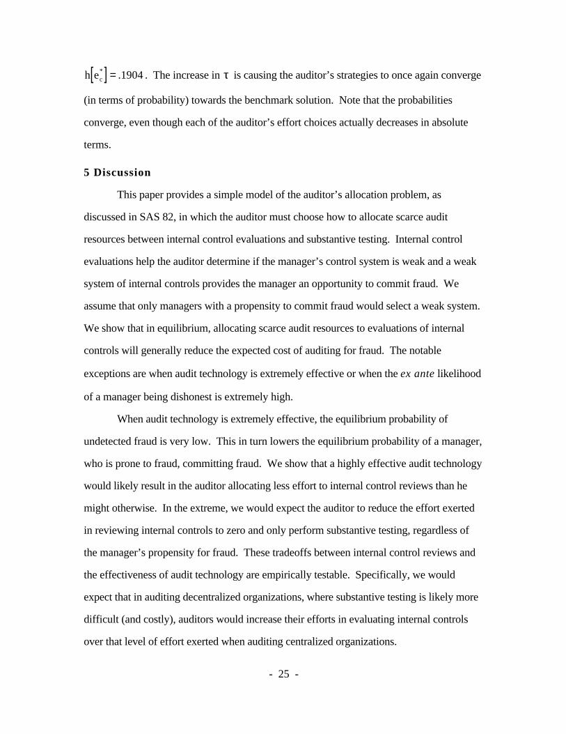
h ec*[ ] = .1904 . The increase in τ is causing the auditor’s strategies to once again converge

(in terms of probability) towards the benchmark solution. Note that the probabilities

converge, even though each of the auditor’s effort choices actually decreases in absolute

terms.

5 Discussion

This paper provides a simple model of the auditor’s allocation problem, as

discussed in SAS 82, in which the auditor must choose how to allocate scarce audit

resources between internal control evaluations and substantive testing. Internal control

evaluations help the auditor determine if the manager’s control system is weak and a weak

system of internal controls provides the manager an opportunity to commit fraud. We

assume that only managers with a propensity to commit fraud would select a weak system.

We show that in equilibrium, allocating scarce audit resources to evaluations of internal

controls will generally reduce the expected cost of auditing for fraud. The notable

exceptions are when audit technology is extremely effective or when the ex ante likelihood

of a manager being dishonest is extremely high.

When audit technology is extremely effective, the equilibrium probability of

undetected fraud is very low. This in turn lowers the equilibrium probability of a manager,

who is prone to fraud, committing fraud. We show that a highly effective audit technology

would likely result in the auditor allocating less effort to internal control reviews than he

might otherwise. In the extreme, we would expect the auditor to reduce the effort exerted

in reviewing internal controls to zero and only perform substantive testing, regardless of

the manager’s propensity for fraud. These tradeoffs between internal control reviews and

the effectiveness of audit technology are empirically testable. Specifically, we would

expect that in auditing decentralized organizations, where substantive testing is likely more

difficult (and costly), auditors would increase their efforts in evaluating internal controls

over that level of effort exerted when auditing centralized organizations.

- 26 -

When the ex ante likelihood of a manager being dishonest is extremely high, we

show that the cost savings from allocating resources to internal control reviews is

diminished. While this result may appear counterintuitive, it follows directly from Bayes’

Rule. The information content of learning that internal controls are weak does not

substantially update the auditor’s expectations regarding fraud, thus, does not substantially

reduce the required level of substantive testing. This result is also empirically testable.

Specifically, we would expect that auditors would reduce their efforts in evaluating internal

controls and increase substantive testing in industries prone to high levels of fraud.

A limitation of our study is that we do not allow the manager to select the

information system quality. Rather, we assume that evidence of a weak system is fully

revealing. While we believe that allowing system quality to vary could alter our results, we

expect that the implications of the study would be similar. Future research may be able to

identify how noisy information about system quality, rather than a fully revealing signal,

would effect the auditor’s effort level in fraud detection.

- 27 -

References

American Institute of Certified Public Accountants, “Statement on auditing standardsNumber 82 - consideration of fraud in a financial statement audit, 1997.

Caplan, D. “Internal controls and the detection of management fraud,” working paper,Columbia University (1997).

Chiang, A. Fundamental Methods of Mathematical Economics, Third edition,MacGraw-Hill, 1984.

Finn, M. and M. Penno “Real-time inspection games with varying levels of commitment,”working paper, Northwestern University, 1996.

Newman, P. and J. Noel “Error rates, detection rates, and payoff functions in auditing,”Auditing: A Journal of Practice and Theory, pp. 50-66, 1989 (Supplement).

, J. Park and R. Smith “Allocating internal audit resources to minimize detection riskdue to theft,” Auditing: A Journal of Practice and Theory, Forthcoming, 1998.

, S. Rhoades, and R. Smith “Allocating audit resources to detect fraud,” Review ofAccounting Studies, pp. 161-182, 1996.

Park, J. “Strategic audit timing plans,” unpublished dissertation, University of Texas,1995.

Patterson, E. “Strategic sample size choice in auditing,” Journal of Accounting Research,pp. 272-293, 1993.

Shibano, T. “Assessing audit risk from errors and irregularities,” Journal of AccountingResearch pp. 110-147, 1990 (Supplement).

- 28 -

fraud

no fraud

no fraud

dishonestθ

honest1 − θ( )

fraud

αb

αg

e

e

F 1 − d e[ ]( ) − PDd e[ ] , − e − D 1− d e[ ]( )( )

−PDd e[ ] , − e − D 1− d e[ ]( )( )

0,−e( )

0,−e( )

Figure 1Benchmark Model

- 29 -

type

(hon

est,

dish

ones

t)de

term

ined

.th

is in

duce

ssy

stem

cho

ice

audi

tor

choo

ses

syst

emev

alua

tion

effo

rt

audi

tor

lear

ns(o

r do

es

not l

earn

)m

anag

er is

fr

aud-

pron

e (i

f he

is)

audi

tor

(bas

ed o

n re

sults

of

inte

rnal

co

ntro

l eva

luat

ion)

ch

oose

s su

bsta

ntiv

e te

stin

g

man

ager

cho

oses

frau

d or

no

frau

d (w

ithou

t kno

win

g th

e re

sults

of

the

audi

tor's

inte

rnal

co

ntro

l eva

luat

ion

audi

tor

disc

over

sfr

aud

if it

occ

urre

dpr

obab

ilist

ical

ly

Figu

re 2

Tim

elin

eT

wo

-sta

ge m

odel

- 30 -

natu

reau

dito

ras

sess

men

tef

fort

natu

re(c

ontr

olas

sess

men

t)

audi

tor

effo

rtm

anag

er

eC e C

e W e0 e 0

0,−

e0

−e c

()

1

he c[

]

1−

he c

[]

frau

d

no f

raud

frau

d

no f

raud

no f

raud

dish

ones

tθ

F1

−d

e w[]

()−

de w

[]P

D,−

e w−

e c−

D1 −

de w[

](

)(

)

F1

−d

e 0[]

()−

de 0[

]PD,−

e0

−e c

−D

1−d

e 0[

](

)(

)

0,− e

w−

ec

()

hone

st1

−θ

()

frau

d

αb α

b

α g

0,− e

c−

e0

()

− PD

de 0[

],−

D1

−d

e 0[]

()−

ec

−e

0(

)

Figu

re 3

Gam

e T

ree

Tw

o-St

age

Mod

el

- 31 -

Proof of Proposition 1

First, suppose that (21) and (22) define the auditor’s detection strategy.

Substituting (21) and (22) into (8) yields:

−h ec[ ] 1 −θ( )PDα b + h ec[ ] 1 − θ( )PDαb = 0 . (A1)

In other words, for the manager, any choice of αb is optimizing if the auditor is choosing

ew and e0 in accordance with (21) and (22). In particular, αb* in (20) is optimizing, as

long as it satisfies: αb* =

F + PD

Dτθ PD

∈ 0,1[ ] .

Now consider the auditor’s problem. Suppose the auditor observes a weak system

of internal controls and knows that the manager is dishonest. In this case, the auditor must

(conditionally) choose ew to satisfy (15). If the manager is choosing αb* as in (20), the

auditor’s FOC in (15) can be rewritten:

θ PD − F + PD( ) 1 − d ew[ ]( ) = 0 , (A2)

which implies that d ew[ ] is characterized by (21). Using the same approach, we find that

αb* =

F + PD

Dτθ PD

implies that the auditor’s choice of e0* in (22) satisfies the auditor’s FOC. In

addition, since these decisions must be sequentially rational, the second order conditions in

(16) and (19) are sufficient to ensure that these choices are optimal. n

Proof of Proposition 2

Suppose there exists a value, e c > 0, which satisfies (24). We need to show that

this value defines the equilibrium choice of the auditor in the second stage of the game.

Since (24) is the solution to the auditor’s FOC, we must only show that the second order

conditions for an optimum are satisfied.

- 32 -

We begin by constructing the 3X3 Hessian matrix of second-order partials (for the

auditor). Denoting the auditor’s payoff in (12) as A, this matrix is:

H =

∂2A

∂ec2

∂2A

∂e c∂ew

∂2A

∂e c∂e0

∂2A

∂e c∂ew

∂2A

∂ew2

∂2A

∂e0∂ew

∂2A∂e c∂e0

∂2A∂e0∂ew

∂2A∂e0

2

. (A3)

We will also substitute in the equilibrium first-order condition: ∂A

∂e c

= 0 . The first principal

minor is given by the first row/first columne element of H. Substituting ∂A

∂e c

= 0 into

∂2A

∂ec2 = 0 , we obtain:

h'' ec[ ]h' e c[ ] < 0 . The second principal minor is:

∂2A

∂ec2

∂2A

∂ew2 −

∂2A

∂e c∂ew

2

.

Substituting ∂A

∂e c

= 0 into this expression, we obtain: −θ2 d ew[ ] − d e0[ ]( )h e c[ ]h'' e c[ ]1 − d ew[ ]( ) 1+θh' ec[ ] ew − ec( )( ) .

Since ew* > e0

* (see corollary 1), d ew[ ] must be greater in equilibrium than d e0[ ] . Hence,

this expression must be positive. The third and final principal minor is the determinant of

H. Without replicating the cumbersome details (available from the author), we observe

than the third principal minor is negative if and only if (24) is satisfied. n

Proof of the comparative static results:

The comparative static results are obtained by using the Implicit Function Theorem over the

system of equations. We begin by building a vector of first order conditions. We will

simplify the process by ignoring the first order condition in (15) and focusing on the other

three FOCs. We will substitute this condition in afterwards. The vector, FOC, is:

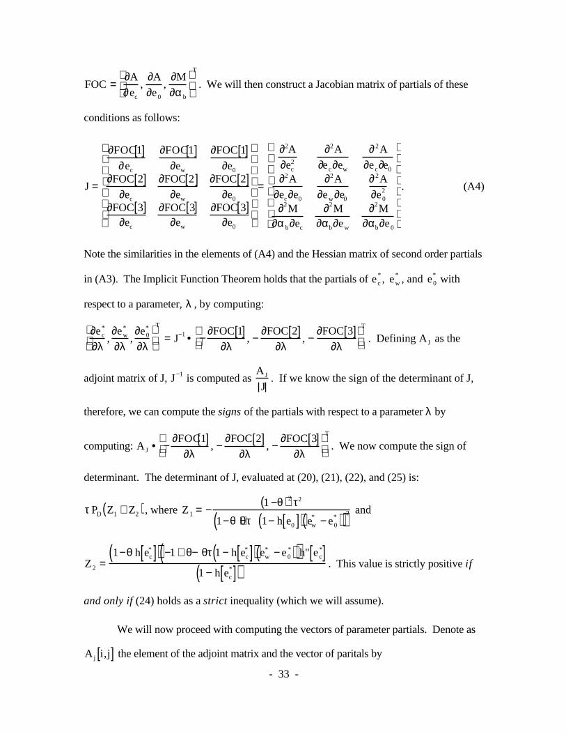
- 33 -

FOC =∂A

∂ec

,∂A

∂e0

,∂M

∂αb

T

. We will then construct a Jacobian matrix of partials of these

conditions as follows:

J =

∂FOC1[ ]∂ec

∂FOC1[ ]∂ew

∂FOC 1[ ]∂e0

∂FOC 2[ ]∂ec

∂FOC 2[ ]∂ew

∂FOC 2[ ]∂e0

∂FOC 3[ ]∂ec

∂FOC 3[ ]∂ew

∂FOC 3[ ]∂e0

=

∂2A

∂ec2

∂2A

∂e c∂ew

∂2A

∂e c∂e0

∂2A

∂ec∂e0

∂2A

∂ew∂e0

∂2A

∂e02

∂2M∂αb∂ec

∂2M∂αb∂ew

∂2M∂αb∂e0

. (A4)

Note the similarities in the elements of (A4) and the Hessian matrix of second order partials

in (A3). The Implicit Function Theorem holds that the partials of e c* , ew

* , and e0* with

respect to a parameter, λ , by computing:

∂e c*

∂λ,∂ew

*

∂λ,∂e0

*

∂λ

T

= J−1 • −∂FOC 1[ ]

∂λ, −

∂FOC 2[ ]∂λ

, −∂FOC 3[ ]

∂λ

T

. Defining A J as the

adjoint matrix of J, J−1 is computed as A J

J. If we know the sign of the determinant of J,

therefore, we can compute the signs of the partials with respect to a parameter λ by

computing: A J • −∂FOC1[ ]

∂λ, −

∂FOC 2[ ]∂λ

, −∂FOC 3[ ]

∂λ

T

. We now compute the sign of

determinant. The determinant of J, evaluated at (20), (21), (22), and (25) is:

τ PD Z1 + Z2( ), where Z1 = −1 −θ( )2 τ2

1−θ +θτ 1− h e0[ ]( ) ew* − e0

*( )( )2 and

Z2 =1−θ h ec

*[ ]( ) −1 + θ− θτ 1 − h ec*[ ]( ) ew

* − e0*( )( )h" e c

*[ ]1 − h ec

*[ ]( ) . This value is strictly positive if

and only if (24) holds as a strict inequality (which we will assume).

We will now proceed with computing the vectors of parameter partials. Denote as

A j i,j[ ] the element of the adjoint matrix and the vector of paritals by

- 34 -

FOCλ = −∂FOC 1[ ]

∂λ, −

∂FOC 2[ ]∂λ

, −∂FOC 3[ ]

∂λ

. Equations (A5) through (A9) compute the

vectors of partials.

FOCθ = −1

θ, −

1

θ, 0

. (A5)

FOCF = 0,0, −1 + d e0*[ ] 1 − h e c

*[ ]( ) + d ew*[ ]h e c

*[ ]{ } . (A6)

FOCPD = 0, 0, d e0*[ ] 1 − h e c

*[ ]( ) + d ew*[ ]h ec

*[ ]{ } . (A7)

FOCD = 0,0,0{ }. (A8)

FOCτ =θ d ew

*[ ]− d e0*[ ]( )h' e c

*[ ]τ2 1 − d ew

*[ ]( ) , 0, 0

.23 (A9)

Now we proceed to determine the signs in table 2.

∂e c*

∂θ= −

1

θ1,1,0[ ]• A j 1,1[ ],A j 1,2[ ],A j 1,3[ ][ ] = −

1

θA j 1,1[ ] + A j 1,2[ ]( )

Using (21), (22), and (25):

A j 1,1[ ] + A j 1,2[ ] =θτ2 τ 1+ θh ec

*[ ]2( ) e0* − ew

*( ) + h ec*[ ]PD −1 +θ − 1+ θ( )τ e0

* − ew*( )( )( )

−1 +θ −θτ 1− h e c*[ ]( ) e0

* − ew*( )( ) .(A10)

Using (25), we know that this must be positive if the numerator is negative. We establish

that it is negative by looking at the sign numerator over the range of τ . The numerator is

negative if τ 1+θ h ec*[ ]2( ) e0

* − ew*( ) + h e c

*[ ]PD −1 +θ − 1 + θ( )τ e0* − ew

*( )( )( ) (A11)

23 For all other comparative statics, the derivatives with respect to e

w

* and e

0

* are the same as for d e

w

*[ ] and

d e0

*[ ] since the value of d[e] does not depend upon anything except τ and e. For this comparative static,

- 35 -

is negative. Suppose τ = 0 . This expression is computed as: −h ec*[ ]PD 1−θ( ) < 0 . Next,

compute the derivative of the expression with regards to τ . This derivative is:

1 − h e c*[ ]( ) 1−θh ec

*[ ]( ) e0* − ew

*( ) < 0 . Hence (A10) must be positive. This implies that

∂e c*

∂θ< 0 .

∂ew*

∂θ= −

1

θAj 2,1[ ] + A j 2,2[ ]( ) . Since A j 1,2[ ] is zero and A j 2,2[ ] =

1

τDet J[ ] ,

A j 2,1[ ] + A j 2,2[ ] = Aj 2,2[ ] > 0 , which implies that ∂ew

*

∂θ< 0 .

∂e0*

∂θ= −

1

θA j 3,1[ ] + A j 3,2[ ]( ) . Computing A j 3,1[ ] + A j 3,2[ ] and substituting in (21) and

(22), we obtain:

1 −θ( )h' e c*[ ] τ 1 − h e c

*[ ]( ) − 1−θ( )h' ec*[ ]( ) −θ 1− h ec

*[ ]( )h ec*[ ]h'' e c

*[ ]Z3 , (A12)

where: Z3 = −1 +θ− θτ 1− h e c*[ ]( ) e0

* − ew*( )( ). Next we rewrite (our strict version of)

constraint (24) as: h'' ec*[ ] = −

A + 1 − θ( )2τ2 1 − h ec*[ ]( )

1 −θh e c*[ ]( ) 1 −θ 1 − τ 1− h ec

*[ ]( ) e0* − ew

*( )( )( )3 (A13)

where A is the positive real number which converts (24) to an equality. Substituting

(A13) and (25) into (A12), we obtain an expression with the numerator:

1 −θ( )θτ2 1− h ec*[ ]( )PD τ e0

* − ew*( ) 1 +θh e c

*[ ]2( ) + h e c*[ ] −1 +θ− 1 + θ( )τ e0

* − ew*( )( )( )

− AθPDh e c*[ ]

. (A14)

however, we are actually computing d d e *[ ]

d τ=

∂ d e[ ]∂ τ e*

+∂ d e*[ ]

∂ e*

∂ e *

∂ τ e*

. As we are actually focused on

d ew

*[ ] and d e0

*[ ] converging to d e*[ ] we are not concerned with this technical issue.

- 36 -

(A14) is shown to be negative in exactly the same way that (A11) was shown to be

negative. The denominator of the expression is:

1 − h e c*[ ]( ) 1−θh ec

*[ ]( ) −1+ θ− θτ 1 − h ec*[ ]( ) e0

* − ew*( )( )2

, which must clearly be positive.

Hence, ∂e0

*

∂θ> 0 .

Next consider the signs of ∂e c

*

∂F,

∂ew*

∂F,

∂e0*

∂F,

∂e c*

∂PD

,∂ew

*

∂PD

, and∂e0

*

∂PD

. Note from (A6) and

(A7) that only the last column of A J is important. In addition, the last element in the vector

(A6) is always negative and the last element in (A7) is always positive since

d e0*[ ] 1 − h e c

*[ ]( ) + d ew*[ ]h ec

*[ ] must be strictly between d e0*[ ] and d ew

*[ ] . As a result, we

conclude:

sign∂e c

*

∂F

= −sign

∂e c*

∂PD

= sign A j 1,3[ ][ ]

sign∂ew

*

∂F

= −sign

∂ew*

∂PD

= sign A j 2,3[ ][ ]

sign∂e0

*

∂F

= −sign

∂e0*

∂PD

= sign A j 3,3[ ][ ]

The sign of A J 1,3[ ] is zero. Using (21), (22), (25) and (A13), the sign of

A J 2,3[ ] = AJ 3,3[ ] = −A

1− h e c*[ ]( ) −1 +θ−θτ 1− h e c

*[ ]( ) e0* − ew

*( )( )2 < 0 . (A15)

As a result, we conclude that:

∂e c*

∂F=

∂e c*

∂PD

= 0 , ∂ew

*

∂F=

∂e0*

∂F> 0 , and

∂ew*

∂PD

=∂e0

*

∂PD

< 0 .

Clearly from (A8), changes in D do not affect the auditor’s choices at all.

- 37 -

Finally, from (A9), we observe that only the first column of the adjoint matrix matters in

determining the signs of ∂e c

*

∂τ,

∂ew*

∂τ, and

∂e0*

∂τ. The first element of FOCτ is clearly

positive. So we conclude that:

sign∂e c

*

∂τ

= sign A j 1,1[ ][ ]

sign∂ew

*

∂τ

= sign A j 2,1[ ][ ]

sign∂e0

*

∂τ

= sign A j 3,1[ ][ ]

Using (21), (22), and (25), A J 1,1[ ] = −τ2 1−θh e c*[ ]( )PD < 0, which implies

∂e c*

∂τ< 0 .

A J 2,1[ ] = 0. And using (21), (22), (24), and (25), we know that

A J 3,1[ ] =1−θ( )τ2PD

1−θ +θτ 1− h e c*[ ]( ) e0

* − ew*( )( ) > 0 . n