The Institutional Causes of China’s Great Famine, 1959-1961∗

Xin Meng Nancy Qian Pierre Yared

July 31, 2013

Abstract

This paper studies the causes of China’s Great Famine, during which approximately

thirty million individuals died in rural areas. We document that average rural food retention

during the famine was too high to generate a severe famine without rural inequality in food

availability; that there was significant variance in famine mortality rates across rural regions;

and that rural mortality rates were positively correlated with per capita food production, a

surprising pattern that is unique to the famine years and one that cannot be explained by

existing theories of the causes of famine. We provide evidence that an inflexible and progres-

sive government procurement policy where procurement was increasing in target production

was necessary for generating this pattern.

Keywords: Famines, Modern Chinese History, Institutions, Central Planning

JEL Classification: P2, O43, N45

∗We are indebted to Francesco Caselli, an anonymous co-editor and seven anonymous referees for invaluablesuggestions. We also thank Daron Acemoglu, Philippe Aghion, Alberto Alesina, Abhijit Banerjee, Robin Burgess,Andrew Foster, Claudia Goldin, Mikhail Golosov, Avner Greif, Rick Hornbeck, Chang-tai Hsieh, Dean Karlan,Michael Kremer, James Kung, Naomi Lamoureaux, Christopher Leighton, Cormac O’Grada, Suresh Naidu, EmiNakamura, Nathan Nunn, Gerard Padro-i-Miquel, Chris Udry, Dennis Yang and Fabrizio Zillibotti for their com-ments; the participants at the Berkeley Development Seminar, Kiel Institute of International Economics, UCLAApplied Economics Seminar, Stanford Economic History Seminar, University of Texas at Austin Applied MicroSeminar, University of Toronto Applied Micro Seminar, Tsinghua University Economics Seminar, the AppliedWorkshop at CCER PKU, the Economics Workshop at Hong Kong University, the Applied Micro Seminar at theChinese University of Hong Kong, Yale University Macro Lunch and Harvard History Tea, and the participantsat BREAD-CIPREE, CEPR-DE, the NBER Summer Institute for Economic Growth, the University of HoustonHealth and Development Conference, and the Conference on Fetal Origins and Famines at Princeton Universityfor useful comments; and Louis Gilbert, Sara Lowes, Ang Sun, David Liu, Jaya Wen, Yiqing Xu and Kai Yanfor excellent research assistance. We acknowledge the Harvard Academy Scholars program for financial support.Please send comments to any of the authors: xin.meng@anu.edu.au, nancy.qian@yale.edu, pyared@columbia.edu.

1 Introduction

During the twentieth century, approximately seventy million people perished from famine.1 This

study investigates the causes of the Chinese Great Famine (1959-61), which killed more than any

other famine in history: approximately thirty million individuals, most of whom were living in

rural areas, perished in just over three years.

The existing literature on the causes of the Great Famine has formed a consensus that a

fall in aggregate food production in 1959 followed by high government procurement from rural

areas were key contributors to the famine.2 In this paper, we argue that these factors could

not have caused the famine on their own because average rural food availability was too high to

generate famine. Thus, any explanation of the famine must account for within-rural variation

in food availability and famine mortality. Motivated by this reasoning, we analyze the spatial

relationship between agricultural productivity and famine severity. We find a surprising positive

correlation between mortality rates and productivity across rural areas during the famine. We

provide evidence that an inflexible and progressive government procurement policy was necessary

for generating this pattern and that this policy was a quantitatively important contributor to

overall famine mortality.

Our study proceeds in several steps. The first step is to document that, even post-procurement,

rural regions as a whole retained enough food to avert mass starvation during the famine. Since

the entire rural population relied on rural food stores, we compare the food retained by rural

regions after procurement to rural per capita food requirements. Using historical data on aggre-

gate food production, government procurement and population (adjusted for the demographic

composition), we find that the average rural food availability for the entire rural population was

almost three times as much as the level necessary to prevent high famine mortality. We reach

these conclusions even after constructing the estimates to bias against finding sufficient rural

food availability. Our findings are consistent with existing estimates of high rural food avail-

ability for rural workers and imply that the high level of famine mortality was accompanied by

significant variation in famine severity within the rural population. In other words, there must1See Sen (1981) and Ravallion (1997) for estimates of total famine casualties.2For a detailed discussion, see Section 2.

1

have been some factor that caused a large rise in the inequality of access to food across the rural

population, which, in turn, resulted in significant variance in mortality outcomes across the rural

population.

The second step is to verify this conjecture by showing that the increase in mortality rates

during the famine was accompanied by an increase in the variance of mortality across the rural

population. Since the historical mortality data are limited to total mortality at the regional level,

we focus on spatial variation in mortality. We find that mortality rates across provinces varied

much more during the famine than in other years. To investigate whether this pattern remains

true at a more disaggregated level, we also use the birth-cohort sizes of survivors observed in

1990 to proxy for famine severity at the county level.3 This is based on the logic that famine

increases infant and early childhood mortality rates and lowers fertility rates such that a more

severe famine results in smaller cohort sizes for those born shortly before or during the famine.

The data show that there is much more variation in cross-county birth-cohort sizes for famine

birth-cohorts relative to non-famine birth-cohorts. This is true both across and within provinces.

These findings imply that an explanation of the famine will need to explain the increase in both

the mean and the variation in mortality rates in rural regions during the famine.

Third, we document the empirical relationship between mortality rates and productivity

across rural areas. We find that across rural regions, famine severity is positively correlated

with per capita food production, a pattern that is unique to the famine era. This surprising

correlation holds at the province-level, where we use mortality rates to proxy for famine severity

and per capita grain production data to measure productivity.

We acknowledge that these estimates could be biased by contemporaneous misreporting of

the historical data for production and mortality. For example, the Chinese government during

the Great Leap Forward era (GLF 1958-61) was known to have over-reported grain production.

Hence, one may be concerned that the positive correlation between mortality and reported pro-

duction reflects the over-reporting of production in the more famine-stricken regions. To address

this, we construct a measure of productivity that does not rely on production data from the

GLF era, but instead relies on data that were not known to have been manipulated, such as3There is no county-level historical data on mortality rates.

2

historical weather conditions and geo-climatic suitability, or data that would have been easy to

correct after the GLF such as total population and total land area, to impute per capita grain

production. To minimize the possibility that our results are driven by misreporting, the main

empirical analysis of the spatial patterns uses the constructed production measure.

In addition, we show that the correlation holds at the county-level (within provinces), where

we use the birth-cohort size of famine survivors to proxy for famine severity, and weather and

suitability to proxy for productivity.4 These additional results allow us to rule out the addi-

tional possibility that the spatial patterns we detect are driven by misreporting of the historical

mortality data.

The fourth step is to examine whether our empirical findings can be explained by existing

theories of the causes of the famine, which have primarily focused on the role that policies specific

to the GLF played in causing the famine. We take the variables for GLF policies used in existing

studies and show that regional GLF intensity cannot explain the patterns we observe in the data

and a new explanation is needed.5 Moreover, we show that productivity explains an order of

magnitude more of the variation in the mortality increase during the famine than GLF intensity.

It follows that explaining the correlation between productivity and famine severity across rural

areas can potentially explain a large fraction of overall famine mortality.

Finally, we provide an explanation for the empirical findings. We argue that the spatial

patterns of famine severity were the result of an inflexible and progressive government procure-

ment policy combined with a fall in per capita production that was roughly proportional for

each region, a fact that we document in the data. In the late 1950s, the central government

procured as much grain as it could from rural areas while leaving rural workers with enough

food to be productive laborers. The procurement policy was progressive as it procured a higher

percentage of total production from more productive areas and inflexible as the government set

each region’s procurement level in advance such that it could not be easily adjusted afterward.

This was because weak state capacity, along with political tensions, made communication chal-4There is no county-level historical grain production data.5Our empirical findings are also inconsistent with the more common market failure interpretation of famines,

whereby mortality is positively correlated with lack of access to food markets. For example, Sen (1981) arguesthat the Bengal Famine (1943) was partly due to the inability of rural wage workers in famine stricken regions tobuy food from regions with surplus production.

3

lenging and hampered the government’s ability to respond quickly to a harvest that was below

their expectations. As a consequence, the level of procurement from a given rural region did

not respond to the actual amount produced, but was instead based on an estimated produc-

tion target established months earlier, where this target was itself based on past production.

After procurement took place, the food retained in a given region would be negatively corre-

lated with the difference between target production and realized production, i.e. the “production

gap”. Since more productive regions experienced a larger absolute production drop while still

remaining more productive relative to less productive regions, the procurement policy caused

more productive regions to experience a larger per capita production gap, subjecting them to

more over-procurement, which in turn, led to less per capita food retention, less per capita food

consumption and higher mortality rates.

To examine the plausibility of our explanation, we test the prediction of our proposed mech-

anism that mortality rates should be positively correlated with the production gap and that

this should be true in all years around during the 1950s and 60s since they were subject to a

similar procurement policy. To estimate the production gap, we construct a measure of target

production that is based on past production and past production growth. The results show that

province-level mortality is positively associated with the production gap, a relationship that is

robust to controlling for GLF intensity and the exclusion of famine years.

Finally, we use a back-of-the-envelope calculation to show that the inflexible procurement

mechanism explains 40-45% of total famine mortality. This result shows that our proposed

mechanism is quantitatively important, and at the same time leaves room for other factors to

contribute to famine mortality. In addition, we use historical province-level procurement data to

provide evidence that the link between the production gap and mortality is driven by government

procurement.

The main challenges for our study are data availability and quality. We address these diffi-

culties by using a large array of data from contemporaneous, archival, Chinese and international

sources. As we discussed earlier, we address the possibility of systematic over-reporting of pro-

duction by constructing a measure of production that does not use GLF-era production data. We

are also able to address potential concerns that mortality rates are misreported by proxying for

4

famine severity with survivor birth cohort size as observed in 1990. The fact that the results are

qualitatively similar across all data sources suggests that the spatial patterns we detect between

agricultural productivity and famine severity are not driven by measurement error.6

This study makes several contributions to the literature. First, it makes progress in under-

standing the root causes of the Chinese Great Famine. It emphasizes that explaining rural food

distribution is necessary for explaining the famine. It is the first to document that famine severity

and regional per capita food production were positively associated. It is also the first to demon-

strate that the inflexibility and the progressiveness of the procurement system are important for

explaining why the famine occurred. Our study supports past studies that find procurement to

be important contributor to famine (e.g., Kung and Lin, 2003; Li and Yang, 2005; Kung and

Chen, 2011). These earlier works do not consider the additional roles of the inflexibility, the

progressiveness of the procurement policy, the proportional fall in output or the importance of

explaining the rural inequality in food consumption. In providing an explanation for the spatial

variation in procurement, our study complements Kung and Lin (2003) and Kung and Chen

(2011), which find that political radicalism was another important contributor to regional pro-

curement levels. In focusing on systemic features of the centrally planned economy, our study

adds to Li and Yang (2005), which examines the causes of production falls during the GLF.7

Our study also improves on past work by constructing GLF-era production from weather and

soil quality data rather than relying on official statistics that may be mismeasured.8

Second, this study adds to the larger literature on famines. Our results are broadly consistent

with Sen’s (1981) thesis that famines are mainly due to food distribution rather than aggregate

food deficits. However, we document spatial patterns in famine severity and food production

that are difficult to explain with market mechanisms. Thus, we expand the literature on the

causes of famine by studying the detailed mechanisms in a non-market context.9 This is an6In addition, in the food accounting exercise, we address the potential misreporting of grain production by

biasing our exercise in the direction of finding a food shortage as much as possible. Despite this, the implied foodsurplus available to avert mortality is so quantitatively large that we believe that it is unlikely that more accuratefigures, should they ever become available, would alter this conclusion.

7See Section 2 for a detailed discussion of past studies.8Our finding that rural food availability is high is consistent with Li and Yang’s (2005) high estimates of caloric

availability during the famine. Their estimates focused on workers, while ours attempt to account for the entirerural population.

9For recent studies on the causes of famines in market economies, see studies such as Burgess and Donaldson(2010), Shiue (2002, 2004, 2005) and OGrada (2007). Also, Dreze (1999) and OGrada (2007) provide overviews

5

important context since approximately sixty percent of all famine deaths in the twentieth century

have taken place in non-market economies (e.g., China’s Great Famine in 1959-61, the Soviet

Famine in 1932-33, and the North Korean Famine in 1992-95).10 In the conclusion, we provide

a speculative discussion of the similarities between the Chinese famine and famines in other

centrally planned economies.

This paper is organized as follows. Section 2 provides a brief historical background. Section

3 estimates rural food availability during the famine. Section 4 documents spatial variation in

famine severity. Section 5 estimates the correlation between famine severity and food produc-

tivity across rural regions. Section 6 explains the empirical patterns with the inflexibility and

progressiveness of the historical food procurement policy. Section 7 offers concluding remarks.

2 Background

2.1 Collective Agriculture

On the eve of the famine, the production, distribution and consumption of food in China were

entirely controlled by the central government. This meant that the government was the sole

insurer of food consumption in the event of a drop in production.11 At the time, approximately

80% of the population worked in agriculture.12 Land reforms that began in 1952 had resulted

in full collectivization by the end of the decade. Private property rights to land and assets

were erased, and markets for private transactions were banned (Fairbank, 1986: p. 281-5).

Agricultural workers were forced to work under constant monitoring and were no longer rewarded

for their marginal input into production (Johnson, 1998). By the end of the 1950s, there were

no wages or cash rewards for effort.13

Grain was harvested and stored communally. Private stores of grain were banned, a rule

of this literature.10Davies and Wheatcroft (2004) estimate that up to 6.5 million died across the Soviet Union during the 1932

famine. In North Korea, it is commonly believed that 2-3 million individuals, approximately 10% of the totalpopulation, died during this famine (e.g., see Haggard and Noland, 2005; and Demick, 2009). There are very fewacademic studies or reliable accounts of details related to this famine.

11See the previous version of this paper, Meng, Qian and Yared (2010), for a detailed discussion on howagricultural collectivization during the 1950s reduced rural households’ ability to smooth consumption.

12We calculate this from data reported by the National Bureau of Statistics (NBS).13See Walker (1965, p. 16-7) for a detailed description of collectivization.

6

that was sometimes enforced with virulent anti-hiding campaigns (Becker, 1996: p. 109). Grain

was procured by the central government from communal depots after the fall harvest around

November. Procured grain was fed to urban workers, exported to other countries in exchange for

industrial equipment and expertise, and stored in reserves as insurance against natural disaster.14

The grain retained by rural regions was fed to peasants in communal kitchens, which were

established so that the collective controlled food preparation and consumption. The government

prevented peasants from migrating, and thus, they were mostly bound to consume the amount

distributed in their collective (Thaxton, 2008: p. 166). When that was insufficient, famine

occurred.

2.2 Famine Chronology

Historians officially define the Great Famine to be three years, 1959-1961, when mortality rates

were the highest. Grain production grew nearly monotonically between 1949 and the beginning

of the GLF. There are a few accounts of production falls in select regions in 1958 and many

accounts of widespread production falls in 1959 and 1960. Famine became widespread when

local stores of the 1959 harvest ran out during the early part of 1960 (Becker, 1996: p. 94;

Thaxton, 2008: p. 207-10). Approximately 30 million people died during the three years in

total. Mortality rates were the highest in the spring and summer months of 1960. The official

explanation provided by the government was bad weather. Recent studies have provided evidence

that the fall in output was also partly due to bad government policies such as the diversion of

resources away from agriculture to industrialization, as well as weakened worker incentives.15

Famine primarily struck the rural areas. Communal kitchens, which survivors recall as having

served large quantities of food, suddenly ran out. Peasants scavenged for calories and ate green

crops illegally from the field (chi qing) when they could (Thaxton, 2008: p. 202). Mortality rates14Historical central planning documents state that approximately 4-5 million tons per year were put into reserves

as insurance against natural disasters (Sun, 1958). During the late 1950s, total grain exports were approximately2% of total production (Walker, 1984: Table 52).

15The policies include labor and acreage reductions in grain production (e.g., Peng, 1987; Yao, 1999), imple-mentation of radical programs such as communal dining (e.g., Chang and Wen, 1997; Yang, 1998), reduced workincentives due to the formation of the people’s communes (Perkins and Yusuf, 1984), and the denial of peasants’rights to exit from the commune (Lin, 1990). Li and Yang (2005) compile province-level panel data on grain pro-duction and attempt to quantify the impact of various potential factors. They find that in addition to weather,the relevant factors were over-procurement and the diversion of labor away from agriculture during the GreatLeap Forward for projects such as rural industrialization.

7

were highest for the elderly and young children (Ashton, Hill, Piazza and Zeitz, 1984: Tables

3 and A7; Spence, 1991: p. 583). Prime-age adults experienced relatively higher survival rates

(Thaxton, 2008: p. 202-10).

Relative to other famines, infectious diseases did not play a major role in causing mortality.

The low level of disease in rural areas during the famine has been attributed to limited population

movements, the prevalent use of DDT prior to the famine, and public health measures taken by

the government during earlier years (e.g., Becker, 1996; Dikotter, 2010: ch. 32; Fairbank, 1986:

p. 279). “People really did die of starvation−in contrast to many other famines where disease

loomed large on the horizon of death” (Dikotter, 2010: p. 285). This is an important point to

keep in mind for calculating the caloric requirement for survival in the Chinese context.16

In recent years, a broad consensus has formed that the government over-procured grain from

rural areas in the fall of 1959, and this exacerbated the production decline and caused the

massive mortality in the spring months of 1960. There are many hypotheses for what led to

over-procurement. The central government placed the blame on local leaders, accusing them of

over-reporting production and consequently leading the central government to over-estimate true

production (Thaxton, 2008: p. 293-9). Recent academic studies find that over-procurement was

driven by multiple factors, including the government’s bias towards providing high levels of food

to urban areas (Lin and Yang, 2000), the political zealousness and career concerns of provincial

leaders (Yang, 1998; Kung and Chen, 2011) and an over-commitment by the central government

to meeting export targets (Johnson, 1998). In addition, some have argued that mortality rates

were exacerbated by food wastage in communal kitchens (Chang and Wen, 1997).

The Chinese government did not begin to systematically respond to the famine until the

summer of 1960, after a large proportion of famine mortality had already taken place. The

response came in several forms. The government returned workers who had been recently moved

to urban areas to assist in industrialization back to their home villages. This was intended to

replenish the greatly weakened and demoralized rural labor force in order to minimize further16Consistent with the belief that infectious diseases were not an important feature of the Chinese Famine,

the data show that famine mortality rates were low in densely populated places such as urban areas and wereuncorrelated with latitude and elevation. Moreover, the results we show in the paper are robust to controlling forpopulation density and its interaction with the famine dummy variable. These correlations are not presented dueto space constraints.

8

falls in production (Li and Yang, 2005; Thaxton, 2008: p. 169). Urban food rations were reduced,

although typically not to below subsistence levels (Lin and Yang, 2000). The government also

abandoned many of the more extreme policies of collectivization (Walker, 1965: p. 83, 86-92;

Thaxton, 2008: ch. 6, p. 215-6). For example, households again stored and prepared their own

food, peasants were again allowed to plant strips of sweet potatoes for their own consumption,

and the government sometimes also turned a blind eye to the black market trading of food across

regions and the illegal consumption of green crops; all this helped preserve lives until the next

harvest (Thaxton, 2008: ch. 4).

These measures could not prevent another decline in production in 1960, this time caused

by the diminished physical capacity of the rural labor force, the lack of organic inputs such as

seeds and fertilizers, which had been consumed during the months of deprivation (e.g., Li and

Yang, 2005), and the consumption by starving peasants of green crops from the field (Thaxton,

2008: p. 202). In 1961, the government finally ended the famine by sending large amounts of

grain into rural areas. Thirty million tons of grain reserves were depleted (Walker, 1984: Ch. 5)

and China switched from being a net exporter to a net importer of grain (Walker, 1984: Table

52). Grain production recovered gradually in subsequent years.

After the famine, procurement rates were kept at a much lower level than during the famine-

era. Official statistics show that aggregate procurement rates declined from approximately 20% of

total production during the famine years to approximately 10% for the next twenty years.17 The

procurement policy remained largely unchanged otherwise. Consistent with the low procurement

levels and the government’s need to feed its growing urban population, China remained a net

importer of grain for several decades. The government did not attempt to re-implement the

extreme policies from the Great Leap Forward (GLF) that were abandoned during the initial

reaction to the famine. China experienced several aggregate production drops of approximately

5%-10% in per capita terms, but never experienced another fall as large as that of 1959 (i.e.,

15%). These factors, together, may explain why there were no subsequent famines in China

(Walker, 1965: ch. 6; Thaxton, 2008: ch. 6).

Politically, the central government engaged in various public campaigns to preserve political17Based on the authors’ calculations. See Section 3 for a description of the data.

9

support during the famine’s aftermath. This was necessary since the famine had primarily

affected the rural population which represented the support base of the communist regime. The

government limited the reports of famine and minimized the mortality numbers; it initiated large-

scale propaganda campaigns such as yiku sitan to convince the population that bad weather and

corrupt bureaucrats were to blame for low production and over-procurement; and it initiated

the fan wufeng movement to allow peasants to punish local leaders for famine crimes (Thaxton,

2008: p. 293-9).

Our study focuses on the three years of the highest mortality rates, 1959 to 1961. Since the

mid-autumn harvest is used to support life for many months of the following year, we focus on

grain production during 1958 to 1960. Note that the chronology of production and mortality

rates portray a consistent picture where roughly constant levels of production in 1958 led to

above-trend mortality rates in 1959, and bigger falls in production in 1959 led to extremely high

mortality rates in 1960. Per capita production stopped changing in 1960 and 1961, during which

time mortality rates declined. Per capita production began to grow in 1962, at which point

mortality rates returned to trend. We document these facts more explicitly in the next sections.

3 Rural Food Availability

The main analysis uses a sample of 19 of the 24 provinces in China during the famine era.

For these provinces, we have data for all of the main variables used in the analysis: mortality,

urban and rural population, production, procurement, weather, and geographical conditions.

For consistency, we use the same sample for all of the estimates presented in the main paper.

Our sample comprises 77% of China’s total population in 1958 and approximately 87% of total

famine mortality.18

18The provinces in our sample are Anhui, Beijing, Fujian, Guangdong, Hebei, Heilongjiang, Henan, Hubei,Hunan, Jiangsu, Jiangxi, Jilin, Liaoning, Shaanxi, Shandong, Shanghai, Shanxi, Tianjin and Zhejiang. Faminemortality was calculated by the authors using mortality data reported by the NBS. In this instance, it is definedas the deaths during the famine that was in excess to the average level of mortality during the five years prior toand after the famine (1953-58, 1962-66). Please see the Online Appendix for a detailed discussion.

10

3.1 Rural Caloric Requirements

To calculate rural food availability when the famine began, we take production as given and

compare it to per capita caloric requirements that we calculate. We focus on a seven-year

window that includes the three official years of famine, 1959-1961, and the two preceding and

two subsequent years. Mortality rates during 1959-1961 depend on the consumption of food

produced during 1958-1960 since harvests are used to support life for a large part of the following

calendar year and only a small part of the current calendar year.

We calculate two benchmarks for caloric requirements: the caloric needs for heavy adult labor

and healthy child development and the caloric needs for staying alive. We use very generous

caloric recommendations provided by the United States Department of Agriculture (USDA) for

the first benchmark, and we calculate the lower benchmark to be 43% of the higher one.19

To adjust for the demographic structure, we use the published tables extracted from the 1953

Population Census. Thus, we assume that the per capita food requirement in 1959 is similar to

that of 1953.20

In the Online Appendix, we describe how we apply demographic data to the USDA guidelines

to calculate the average per capita caloric needs for the population. We estimate that daily

average per capita requirements in 1959 were 1,871 calories for the first benchmark and 804

for the second benchmark. These estimates are lower than average caloric requirements for

adult workers because they also account for young and elderly individuals in the population,

who require fewer calories per person. It is important to note that our estimates are extremely

conservative and constructed to obtain high levels of caloric requirement.

The main caveat in interpreting these estimates is that the demographic structure may have19There is not much evidence for how many calories are needed to stay alive. This is partly because starvation

is typically accompanied by other conditions such as disease, unsanitary conditions, war, etc. All of these otherfactors contribute to mortality, but they are not applicable in our context since rural China had a low levelof endemic disease, had high sanitary standards, and did not experience war. The best evidence we have oncalories and starvation is from the Minnesota Starvation Experiment, where the U.S. military systematicallysubjected military volunteers to high levels of physical exertion, chronic starvation and harsh conditions (e.g.,high temperatures). In these experiments, the lowest level of caloric consumption was approximately 900 caloriesa day. This was far above the level that would cause mortality and the subjects were still required to exercise.Similarly, Dasgupta and Ray (1986), in their well-known paper on nutrition and work, chose the 900 calories perday benchmark as the amount required for an adult male to do some work. For these reasons, we also chose 900calories as the lower benchmark and interpret it as the extreme upper bound of the amount of calories requiredto survive. Since 900 calories is 43% of the level needed for heavy adult labor for prime age men, we assume thesame proportional needs for all other groups.

20See the Online Appendix for a more detailed description.

11

changed between 1953 and 1959 such that per capita requirements were higher in 1959. This is

unlikely because the proportion of elderly and the proportion of children both increased during

1953-59.21 Since the very young and elderly require fewer calories than prime age adults, this

would most likely cause us to over-estimate average per capita caloric needs in 1959.

Applying the 1953 estimates to the years immediately after the famine is more problematic.

Since the young and the elderly were more likely to have perished during the famine, the average

per capita caloric needs during the post-famine years could have been much higher than in 1953.

Hence, the caloric accounting for the years after the famine should be interpreted cautiously.

3.2 Rural Food Availability

Grain production, total population and urban population data are published by the National

Bureau of Statistics (NBS). Note that although the three province-level municipalities were

mostly urban, they still contained significant agricultural populations that engaged in grain

production.22

The data on grain production is not disaggregated by types, which include rice, sorghum

and wheat. Therefore, to convert data for the volume of retained grain into calories, we use the

Chinese Ministry of Health and Hygiene’s (MHH) estimate of calories contained in the typical

mix of grains consumed by an average Chinese worker, and we assume that one kilogram of grain

provides 3,587 calories. Moreover, we assume that individuals subsist solely on grain, which is a

reasonable description of the diet of Chinese peasants in the 1950s (Walker, 1984).

The data for national grain production and total population are displayed in Table 1 columns

(1) and (2). In column (5), we use these data to estimate per capita production, which is then

converted in column (6) into per capita food availability in terms of calories per day using

the MHH’s estimate of calories per kilogram of grain. Aggregate production in column (1) and

estimated per capita food availability in column (6) show that per capita production was roughly

constant between 1957 and 1958. And although production and food availability declined from21Crude demographic projections suggest that between 1953 and 1959, youth dependency (the number of people

aged 0 to 10 per 100 people aged 20 to 64) approximately increased from 90 to 100. The rate of increase wasconstant over time and shows no change during the GLF. Similarly, the dependency ratio of the elderly (thenumber of people over 64 per 100 people aged 20 to 64) was constant over this period. These statistics suggestthat the proportion of prime-age adults in the population was declining (Kinsella, Wan and of the Census, 2009).

22During the 1950s, 34%, 30% and 47% of the populations of Beijing, Shanghai and Tianjin were rural.

12

1958 to 1959, national production provided approximately 2,421 calories per capita in 1959,

which is approximately 300% of the 804 calories necessary for preventing mortality and 129%

of the 1,871 calories required for heavy labor and healthy child development. In other words,

national average food availability based only on production (if the government procured nothing

from rural areas) was about three times the level needed to avoid mortality. Similarly, in 1960,

per capita production was 2,101 calories per day and far above the two caloric requirement

benchmarks.

We examine the amount of rural grain retention by using the production data described

above and national procurement data reported by the Chinese Ministry of Agriculture (1983).

These data have recently been used by Kung and Chen (2011).23 The national procurement rate

presented in column (4) shows that procurement rate in 1958 was around 24% higher than in

1957 ((0.19−0.15)/0.15 = 0.24). Procurement rate in 1959 was around 28% higher than in 1958

((0.24 − 0.19)/0.19 = 0.28). In 1960, procurement declined back to 1958 levels. The latter is

consistent with the fact that the government began to respond to the famine in 1960.

In columns (7) and (8), we deduct government procurement from production and divide it by

the rural population to estimate average rural caloric availability after procurement. Columns

(7) and (8) show that despite the increased procurement rates, rural per capita retention in 1958

and 1959 was far above the two benchmarks for caloric requirements. For example, consider

retention in 1959, which was associated with the year of highest famine mortality (1960). The

rural population was left with roughly 2,329 calories per capita per day. This is approximately

295% of the 804 calories necessary for preventing mortality and 124% of the 1,871 calories

required for heavy labor and healthy child development. In other words, we find that average

rural food availability was almost three times as high as the level required for avoiding mortality

at the peak of the famine. Similarly, in 1960, we find that average rural caloric availability was

approximately 2,168, which is 269% of the requirement for avoiding mortality.24

23The data report gross procurement as well as the amount that is “sold back” to the countryside for eachprovince. We take the difference between these two quantities to compute net procurement for each province. Wethen aggregate it across provinces to compute aggregate procurement.

24Our estimates of per capita rural caloric availability are comparable, though slightly higher than Li and Yang’s(2005) estimate of 2,063 calories per rural worker. The difference arises because our estimates are based on netprocurement while their estimates are based on gross procurement, which is higher. However, both estimatesshow that rural food availability was too high to have caused a famine without the presence of inequality withinthe rural population. Note that Ashton, Hill, Piazza and Zeitz’s (1984) estimates of national per capita food

13

The main caveat for interpreting these estimates is that official data may overstate production

in order to minimize the appearance of failure of GLF agricultural policies. The government

may have also overstated or understated procurement, depending on whether it wished either to

emphasize the successes of the GLF policies for production or minimize the government’s role

in causing the famine. To address this, we have followed recent studies on the famine in using

production and procurement data that was corrected and reported during the post-Mao reform

era, when the government had no incentive to glorify or undermine the GLF. Moreover, as we

have discussed, we make assumptions throughout to bias our calculations towards finding low

rural food availability (and high food requirements).

4 Spatial Variation in Famine Mortality

4.1 Across Provinces

The fact that average rural food retention was too high to inevitably cause such massive famine

mortality implies that famine severity must have varied significantly across the rural population.

To examine this, we follow existing studies in using mortality rates, reported by the NBS, to

proxy for famine severity. Figure 1a plots average mortality rates and the normalized variance

in mortality rates over time (the cross-province standard deviation divided by the cross-province

mean). The normalization of the standard deviation addresses the concern that the standard

deviation can be mechanically positively correlated with the mean. It shows that both the mean

and the variance of mortality rates spike upwards during the famine years.

Note that the historical mortality data do not distinguish between urban and rural popula-

tions, but as most of the famine mortality occurred in rural areas, we can interpret the figure

to reflect patterns of rural mortality.25 Next, we examine the variation across rural populations

availability in 1959 is 1,820 calories per day. This is lower than the estimates from our study because they assumethat the grain remaining after gross aggregate procurement is used to feed the entire population (both urban andrural). In practice, most of the procured grain was used to feed the urban population and the post-procurementretention was used to feed only the rural population. However, even their estimates are near the level for heavylabor and healthy child development, and much higher than the level needed to avoid mortality.

25If we assume that mortality only occurs within the rural population, we can address this issue by normalizingby the rural population (normalized mortality rates = total mortality rates × total population/rural population).Data for total and rural population are also reported by the NBS. This normalization does not change the observedpattern of a spike in the mean and normalized variance of mortality rates during the famine. These estimates areomitted for brevity and are available upon request.

14

explicitly using another data set.

4.2 Across Counties

To examine spatial variation in famine severity at a finer geographic level, we use another proxy

for famine severity: the birth-cohort size of survivors amongst the agricultural population of each

county, constructed from the 1% sample of the 1990 China Population Census.26 Birth-cohort

size is negatively correlated with famine severity as it captures the reduced fertility and increased

mortality caused by the famine. We construct this famine severity index for the county-level,

which is the lowest official administrative division in China.27 In addition to allowing us to

identify rural individuals, this proxy provides several advantages over the mortality rate data.

First, it allows us to disaggregate our analysis to the county-level and examine whether the same

spatial variations observed at the province-level also exist at this lower level of administrative

division. Second, the larger sample size gives our estimation higher statistical power and allows

us to examine famine severity in provinces for which we do not have data from the NBS publi-

cations.28 Finally, this measure of famine severity is not vulnerable to the misreporting caused

by the government’s desire to understate famine severity. Given the focus of our paper on rural

inequality in famine severity, we focus our analysis on agricultural populations.29

The effect of famine can be observed in the birth-cohort size of survivors. Figure 1b plots26Agricultural populations are defined to be households that report as having the official status of an agricultural

household registration. These statuses were assigned in the early 1950s and there was very little mobility frombeing an officially identified agricultural household to a nonagricultural household between then and 1990. Themain distinction for agricultural households is their obligation to deliver a grain tax to the central government,their right to farmland, and their lack of access to urban public goods such as health care, schooling and housing.For these reasons, there is an unwillingness on both the government’s and the farmers’ sides to switch officialstatuses. An alternative way to identify rural populations is to identify everyone living in a non-urban county asrural. This does not affect our results. Due to space constraints we do not report these results with the alternativedata construction. They are available upon request.

27In the famine era, each county had approximately five communes (also known as collective farms), eachcontaining approximately 5,000 households. However, communes were not an official level of government. Weknow of no data that can be disaggregated to the commune level.

28For consistency, we use the same provinces as in our province-level exercise.29Note that policies against labor migration caused there to be very little rural migration between when the

famine occurred and when survivor cohort sizes are measured in our data (West and Zhao, 2000). To checkthat the birth-cohort size of survivors is a good proxy for famine mortality, we compare survivor cohort sizesand mortality rates at the province-level. We find that these two measures are negatively correlated such thathigher mortality rates imply smaller survivor cohort sizes, and the correlation is highly statistically significant.We aggregate birth-cohort sizes to the province and year (birth year) level and regress the log of birth cohort sizeon the log of mortality while controlling for the log of total population and year and province fixed effects. Thecorrelation is -0.28 and statistically significant at the 1% level.

15

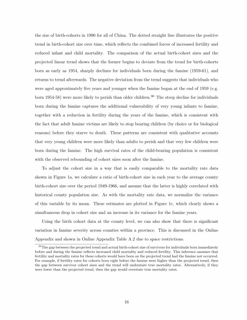
the size of birth-cohorts in 1990 for all of China. The dotted straight line illustrates the positive

trend in birth-cohort size over time, which reflects the combined forces of increased fertility and

reduced infant and child mortality. The comparison of the actual birth-cohort sizes and the

projected linear trend shows that the former begins to deviate from the trend for birth-cohorts

born as early as 1954, sharply declines for individuals born during the famine (1959-61), and

returns to trend afterwards. The negative deviation from the trend suggests that individuals who

were aged approximately five years and younger when the famine began at the end of 1959 (e.g.

born 1954-58) were more likely to perish than older children.30 The steep decline for individuals

born during the famine captures the additional vulnerability of very young infants to famine,

together with a reduction in fertility during the years of the famine, which is consistent with

the fact that adult famine victims are likely to stop bearing children (by choice or for biological

reasons) before they starve to death. These patterns are consistent with qualitative accounts

that very young children were more likely than adults to perish and that very few children were

born during the famine. The high survival rates of the child-bearing population is consistent

with the observed rebounding of cohort sizes soon after the famine.

To adjust the cohort size in a way that is easily comparable to the mortality rate data

shown in Figure 1a, we calculate a ratio of birth-cohort size in each year to the average county

birth-cohort size over the period 1949-1966, and assume that the latter is highly correlated with

historical county population size. As with the mortality rate data, we normalize the variance

of this variable by its mean. These estimates are plotted in Figure 1c, which clearly shows a

simultaneous drop in cohort size and an increase in its variance for the famine years.

Using the birth cohort data at the county level, we can also show that there is significant

variation in famine severity across counties within a province. This is discussed in the Online

Appendix and shown in Online Appendix Table A.2 due to space restrictions.30The gap between the projected trend and actual birth-cohort size of survivors for individuals born immediately

before and during the famine reflects increased child mortality and reduced fertility. This inference assumes thatfertility and mortality rates for these cohorts would have been on the projected trend had the famine not occurred.For example, if fertility rates for cohorts born right before the famine were higher than the projected trend, thenthe gap between survivor cohort sizes and the trend will understate true mortality rates. Alternatively, if theywere lower than the projected trend, then the gap would overstate true mortality rates.

16

5 Spatial Correlation between Famine Severity and Productivity

5.1 Measurement of Province-level Productivity

In this section, we document the empirical relationship between mortality rates and productivity

across rural areas. Our main result points to a positive correlation between mortality and

productivity that is unique to the famine. This correlation holds both at the province level

and the county level.

The NBS provides a measure of grain production at the province level. Our main concern

with this measure is the possibility that, despite their best intentions, statisticians have not been

able to fully correct for government misreporting of production during the GLF. In that case, the

association between productivity and mortality rates during the famine would be confounded by

misreporting.

To address this concern, we construct a time-varying measure of province-level production

that is unlikely to be affected by government misreporting by estimating a production function

using data from non-GLF years (1949-57, 1962-82). We restrict our attention to the years before

1982 so that our estimates can be easily comparable to the results in section 6.3.2. To estimate the

production function, we regress production for province p in year t on the following production

inputs: temperature and its squared term, rainfall and its squared term, grain suitability and its

squared term, rural population and its squared term, total land area and its squared term, and

all combinations of the double interactions of temperature, rainfall, suitability, rural population

and total land area. The production function regression has an adjusted R-squared of 0.93, which

means that the input variables explain 93% of the variation in production.31 Then, we apply

the input data from all years to create a measure of predicted production using the production

function, which we will refer to as “constructed production” henceforth.

The only data from the GLF era that are used for the constructed production measure are the

weather, total area and population variables that are inputs in the production function. Monthly

mean temperature and rainfall are reported by scientific weather stations. Access to these data

was restricted to Chinese scientists until recently. The suitability measure is a time-invariant31We do not report the production function coefficients because of the large number of regressors and the

difficulty in interpreting each coefficient in the presence of interaction effects. They are available upon request.

17

index of a region’s suitability for the cultivation of the main procurement grain crops in China

during the 1950s (rice, sorghum, wheat, buckwheat, barley). The index is produced by the

GAEZ model developed by the Food and Agricultural Organization (FAO), and we assume the

inputs are those that are similar to what was used in China during the 1950s.32 The weather and

suitability variables were never known to have been manipulated by the Mao-era government.

The data for total provincial population and total provincial land area are reported by the post-

Mao NBS. Since these data are difficult to manipulate and easy to correct retrospectively, their

inclusion should not bias the constructed production measure.

Constructed production is similar to reported production. This can be seen in Online Ap-

pendix Figure A.1, which plots constructed grain production against reported grain production

together with the 45-degree line for each of the four years of the GLF. The fact that constructed

and reported production do not line up perfectly on the 45-degree line is consistent with the

presence of misreporting. However, the two measures are highly correlated for all years. To be

cautious, we will use the constructed measure of production for the remainder of our analysis.

The estimates from using reported production data are similar.33

5.2 Province-Level Analysis

With these data, we explore the relationship between food production and famine mortality

rates. To provide a precise estimate of the relationship between per capita food production and

mortality rates, we pool all of the data together and estimate the following equation.

mp,t+1 = αPp,t + βPp,tIFamt + Z′p,tγ + δt + εp,t, (1)

where mp,t+1 is the log number of deaths in province p during year t+ 1; Pp,t is log constructed

grain production; Pp,tIFamt is the interaction of log constructed grain production and a dummy

variable for whether it is a famine year, where IFamt = {0, 1} is a dummy variable that equals 1

if the observation is of year t = 1958, 1959, 1960; Zp,t is a vector of province-year level covariates;32These are based on fixed geo-climatic conditions and the technologies used by Chinese farmers in the late

1950s (e.g., low level of mechanization, organic fertilizers, rain-fed irrigation). See the Online Appendix for adetailed discussion of the weather and suitability data and the construction of province-level measures.

33See Online Appendix Table A.3 for the main results, as well as the previous version of the paper Meng et al.(2010).

18

δt is a vector of year fixed effect; and εp,t is an error term. The vector of covariates in the

baseline specification, Zp,t, includes the log total population, which normalizes our estimates so

that we can interpret them in “per capita” terms. We also control for the log urban population to

ensure that the estimates capture variation driven by rural areas. Year fixed effects control for all

changes over time that affect regions similarly and they subsume the main effect for the famine

year dummy. To address the presence of heteroskedasticity, all of the regressions estimate robust

standard errors.34 Equation (1) estimates the cross-sectional correlation between productivity

and mortality rates for non-famine years as α̂, and the correlation during the famine as α̂+ β.

In Table 2 column (1), we show the cross-sectional correlation between productivity and

mortality rates using a sample for the period 1953 to 1982. Before 1953, mortality data is

not available for all provinces. We end the sample in 1982 so that our estimates will be easily

comparable to the procurement results in Section 6.3.2. In column (2), we restrict the sample

to five years before the famine began until five years after the famine (1953-1965) to show that

our results are driven by the years close to the famine and not spurious correlations long after

the famine ended.35

In both columns (1) and (2), the coefficient for log constructed grain is negative and sta-

tistically insignificant. This means that during normal years, higher production per capita is

uncorrelated with mortality rates. In contrast, the interaction term is positive and statistically

significant at the 1% level, which implies that the relationship between production and mortality

is more positive during the famine years than the non-famine years. The sum of the the inter-

action coefficient and the coefficient for log grain, α̂+ β, is presented at the bottom of the table

along with its p-value. It is positive and statistically significant at the 1% level.

In columns (3) and (4), we show that the results are similar when we use a larger sample of

provinces, where we include the all of the provinces that existed during the famine era except

for Sichuan, for which we have no mortality data. The results with this sample of 23 provinces

are similar. If anything, they are more precisely estimated.34Our results are similar if we estimate wild bootstrapped standard errors that are clustered at the province

level and adjust for the small number of clusters (Cameron, Gelbach and Miller, 2008). These results are notpresented due to space restrictions and are available upon request. The robustness of our estimates to differentlevels of clustering can also be seen later, when we present the county-level analysis that cluster standard errorsat the province level.

35The estimates are similar if we use a sample with a longer time horizon (e.g., until 1998).

19

In columns (5) and (6), we present the results using the reported historical grain production

instead of our main measure of constructed grain production. The estimates are very similar.

Due to space constraints, the remainder of the paper only reports results using the constructed

grain production measures for the main sample of 19 provinces.

To examine whether our estimates are driven by outliers, we plot the residuals of the regres-

sions in column (1) of Table 2. Figure 2 plots the residuals for the interaction of log constructed

grain and the dummy variable for the three famine years. As seen in the regression, the relation-

ship is positive and not driven by outliers.

The results thus far indicate that the positive relationship we observe between grain produc-

tivity and mortality rates during the famine period is very robust. However, the relationship

may change over time during other years. We investigate this in more detail in the next exercise.

In particular, we investigate whether grouping many non-famine years together causes us to cap-

ture spurious changes in the correlation between productivity and mortality rates over time. For

example, the relationship may be very volatile over time and the interaction term may capture

a spurious positive correlation, while the uninteracted grain productivity term averages over the

other positive and negative correlations over time to produce a statistically zero coefficient.

To investigate this possibility, we estimate the yearly correlation between productivity and

mortality rates in the following equation:

mp,t+1 =T∑τ=0

ατPp,τIτt + Z′p,tγ + δt + εp,t, (2)

where mp,t+1, Pp,t, Zp,t, δt, and εp,t are the same as previously defined, and where Iτt = {0, 1}

is a dummy variable that equals one if the observation year t is equal to the year τ , and we no

longer control for the grain productivity main effect because we estimate interaction effects for

each year. This estimate allows the coefficient on productivity to vary for each year. αt is the

cross-sectional correlation between mortality rates and productivity in year t.

Figure 3 plots the estimated coefficients of α̂t and their 95% confidence intervals.36 The

figures show that the correlation between grain productivity and mortality rates is statistically

similar to zero for most years (becoming slightly more negative over time), but spikes upwards36The coefficients and their standard errors are presented in Online Appendix Table A.4.

20

for the first two of the three famine years. The point estimates for the interaction term of log

constructed grain are statistically significant at the 1% level for the peak mortality famine years.

These results show that the positive association between productivity and mortality rates is

unique to the famine. We believe that finding no association between productivity and mortality

for the last famine year (1961 mortality and 1960 production) is consistent with the fact that

the government began to respond to the famine in 1960, since such a response would weaken the

relationship between food production and mortality rates.37

5.3 County-Level Analysis

The province-level analysis faces several limitations. It does not explicitly distinguish between

urban and rural areas; we infer that the cross-province variation reflects differences in rural

mortality rates because we control for urban population. It also does not allow us to examine

whether there is variation across rural areas within a province. Finally, we must take the mortality

data as given and cannot address the possibility that these data may also be measured with error.

We address these concerns by using county-level data that include only agricultural popula-

tions. This allows us to check that there is variation across rural areas and control for province

fixed effects to examine whether there is variation within provinces as well as across provinces.

This exercise also proxies for famine severity using data that was not potentially manipulated by

the Chinese government in order to check that the mortality results are not driven by government

misreporting.

The main dependent variable is thus the alternative proxy for famine severity – birth cohort

size, which is the size of each birth cohort observed in the 1% sample of the 1990 China Population

Census. The main drawback of using these data is that the coefficients of the effect of weather

conditions on survivor birth cohort size are not easy to interpret. Thus, we use birth cohort

sizes to check the robustness of the mortality results. The explanatory variables are measures of

mean spring temperature, rainfall, and grain suitability, which are the disaggregated measures

of the variables used in the province-level production function in Section 5.1. We examine these37The coefficients reflect the cross-section relationship between mortality rates and productivity. Finding no

association means that mortality rates are similar across regions of different productivity. Thus, if the governmentresponds to the famine by giving food or allowing black market “garden” agriculture (see the discussion in Section2), then we will naturally see the link between productivity and mortality rates weaken by the end of the famine.

21

directly (rather than a constructed production measure from the production function) to check

that the earlier results are indeed driven by natural conditions. In this exercise, we interpret the

measures of natural conditions as proxies of productivity.

For consistency, we restrict the sample to the same nineteen provinces used in the province-

level mortality rate analysis. The limited number of historical weather stations additionally

restricts the final sample, which includes 511 counties. Our sample begins with 1950, the first year

for which there is disaggregated weather data, and ends in 1966 to avoid potentially confounding

effects of post-famine political events on fertility.38

We examine the relationship between survivor cohort size and proxies for agricultural pro-

ductivity across rural counties. If the interpretation of our main results are correct, then we

should find similar patterns over time between natural conditions that are advantageous for pro-

duction and survivor birth cohort size – i.e., good conditions should have no relationship or a

positive relationship with birth cohort size for cohorts not affected by the famine, but a nega-

tive relationship for cohorts affected by the famine. Due to space restrictions, we focus on the

year-by-year estimates using equation (2). This differs from earlier estimates in that observa-

tions are now at the county and year level, and we control for log average birth cohort size to

normalize by the population (because there are no data on historical county population sizes

for time of the famine). We also control for province fixed effects to examine whether the same

patterns exist within provinces as across provinces. In one regression, we simultaneously include

the interactions of year dummy variables with each of the three proxies of productivity: mean

log spring temperature, mean log spring rainfall and the suitability for grain cultivation index.

The standard errors are clustered at the county level. The coefficients and standard errors are

reported in Online Appendix Table A.5.

Figures 4a-4c plot the interaction coefficients and their 95% confidence intervals. The pattern

is consistent with the province-level results. To interpret the correlation, recall that being born

in a county that produces high levels of food per capita has two potentially offsetting effects. On38See the Online Appendix for a detailed description of the weather and stuiability data. For example, the

Cultural Revolution (1966-76) caused political disruptions that may have delayed fertility. This is less of an issuefor the province-level mortality estimates because this revolution was not associated with abnormal mortalityrates. The results are similar if we extend the panel to include those born after 1966. They are not reported dueto space constraints, but are available upon request.

22

the one hand, higher food availability may cause higher fertility and lower mortality rates, which

increases the cohort sizes of survivors. On the other hand, these individuals are exposed to a

more severe famine at very young ages, which reduces the cohort size of survivors. Similarly, for

the cohort born during the famine, the more severe famine faced by women of child-bearing age

may reduce fertility. Therefore, finding a negative correlation between cohort size and natural

conditions that are good for production implies that the negative effects of famine exposure

outweigh the positive effects.

Similarly, being born in a productive region has offsetting effects on survivor birth-cohort

size for those born after the famine. On the one hand, survivors living in productive regions

likely had access to more food after the famine relative to less productive regions.39 This could

speed the recovery from famine, increase fertility, reduce infant mortality, and thereby, increase

survivor cohort sizes. On the other hand, famines of greater severity in productive regions mean

that these regions suffer larger population losses, which result in a smaller population base for

bearing and rearing children after the famine. The finding that the correlation between survivor

birth-cohort sizes and natural conditions are zero or positive for those born after the famine

implies that the positive effects outweigh or cancel the negative effects. This is not altogether

surprising since individuals of child bearing age suffered the least from famine and are believed

to have emerged relatively intact.

These results provide strong support that insights from our main findings are not driven by

measurement error in either historical mortality or constructed production data. Moreover, they

also show that the same patterns that exist across provinces also exist across counties within

provinces and motivate us to develop an explanation that is consistent with variation at high

and low levels of government administration.40

39Recall from Section 2 that many of the GLF policies were lifted in response to the famine. If people can eatwhat they produce, then there will naturally be more food per capita in regions with good natural conditions.In addition, our hypothesis that the inflexible grain procurement policy caused the spatial patterns betweenproductivity and famine severity predicts that those living in more productive regions have more food per capitaduring normal years. See Section 6 for details.

40The results are similar when we do not control for province fixed effects, or when we control for province-yearfixed effects to control for time-varying changes across provinces such as political leadership. They are reportedin an earlier version of the paper (Meng et al., 2010).

23

5.4 Controlling for Political Factors

The three years of high famine mortality occurred during the GLF, a four-year period beginning

in 1958 when many misguided policies were often carried out with extreme zealousness. The

implementation of these policies is often thought to be a contributing factor to both the produc-

tion drop and the subsequent mortality rates during the famine. It is natural to wonder whether

more productive regions implemented GLF policies more zealously, which caused higher food

procurement and thereby higher famine severity.

We investigate this alternative hypothesis by examining the correlations between productiv-

ity and proxies for GLF zealousness that past studies have found important. We regress log

per capita grain production on these variables for one cross-section of provinces for the three

famine years. The GLF variables are not available for all of the provinces in our sample, so

for consistency, we restrict the sample to observations for which all of the GLF variables are

reported. These comprise an unbalanced panel of up to seventeen provinces.

First, we follow Li and Yang (2005) and proxy for zealousness with a reduction in the ar-

eas sown for grain and an increase in steel production, since the GLF diverted resources from

agriculture into manufacturing. For ease of interpretation, we construct each variable so that

an increase in the value corresponds to an increase in zealousness. Thus, the variable for sown

area growth is actually the sown area growth multiplied by negative one.41 Table 3 columns (1)-

(2) show that the coefficients for the negative growth in per capita area sown and the positive

growth in per capita steel production are both statistically insignificant. Second, we proxy for

zealousness with the participation rate in communal dining halls (Yang, 1998). By the eve of the

famine, almost all workers ate in communal dining halls. However, past studies, such as Yang

(1998), have argued that communal dining participation rates during the mid-1950s, before the

famine, can be used as a proxy for GLF zealousness. Using the data reported by Yang (1998) on

GLF communal dining participation rates across provinces during the years before the famine,

column (3) shows that participation rates are negatively correlated with productivity. The esti-

mate is statistically significant at the 1% level.42 Third, we use Kung and Chen’s (2011) proxy41We use the same NBS data as in Li and Yang (2005).42Yang (1998) does not report dining hall participation rates for the urban municipalities. To maximize sample

size, we expand this sample by assuming that all workers in the three municipalities ate in communal dining

24

of zealousness, the magnitude of the Anti-Right purges that occurred in 1957, as an explanatory

variable.43 Column (4) shows that this variable is negatively correlated with productivity and

statistically significant at the 1% level. Fourth, we proxy for zealousness with a dummy vari-

able for whether a province was “liberated” by the Communist Party after the official national

liberation date of October 1, 1949. Studies such as Yang (1998) and Kung and Lin (2003) find

that provinces that were liberated after the national liberation date were more likely to appoint

politically zealous leaders. The estimate in column (5) shows that being liberated after the na-

tional date is negatively correlated with productivity. The estimate is statistically significant at

the 1% level.44

In column (6), we include all of these controls in one regression to address the possibility

that they are correlated. When we do this, the positive correlation between the growth in steel

production and grain productivity becomes significant at the 10% level, which suggests that

productive areas may have promoted GLF policies for increasing industrial production more

enthusiastically. At the same time, the negative association of productivity with the percent

of purges during the Anti-right movement (which is only significant at the 20% level) and the

negative association between late liberation and productivity (which is significant at the 1% level)

suggest that productive areas engaged in other GLF policies less intensely. Taken together, the

estimates suggest that GLF policies, as a whole, were not systematically enforced more intensely

in productive regions.

To address the possibility that the lack of statistical significance may be due to the large

number of explanatory variables used in a relatively small sample, we alternatively control for

the principal component of the GLF proxy variables in column (7). The coefficient for this

parsimonious control is negative in sign and statistically significant at the 1% level. Note that

halls, which is motivated by the facts that almost all non-agricultural workers ate in dining halls and that themunicipalities were very urbanized.

43We use the measure of the percent of the total population that is purged (e.g., total purges divided by totalpopulation). We thank the authors of this paper for generously sharing their data with us. In their paper, theyfound that in the cross-section, the number of purges in 1957 is correlated with higher grain procurement duringthe famine.

44We expand the data sample of these previous studies to cover all provinces in our study by collecting liberationdates and months from a Chinese publication with the title that translates into the Report on the Liberation ofthe Peoples Republic of China. It is housed in the archives of the National Library in Beijing. The results aresimilar with other measures of liberation date (e.g., number of months before or after the national liberation, rankof liberation date). Chinese reference names are available upon request.

25

the magnitude and sign of the component coefficient is difficult to interpret. We address this

difficulty with the next set of results. Also note that the results are similar if we control for year

fixed effects.

Another way to show that the positive association between mortality and productivity is not

driven by GLF factors is to show that it is robust to controlling for GLF intensity. To maximize

power, we first control for the principal component of the GLF factors. Note that since we

do not have GLF variables for all of the provinces in our sample, the number of observations is

reduced for this exercise. Column (1) of Table 4 presents the baseline estimates on this restricted

sample. The estimates are very similar to the results with the full sample. Column (2) shows that

adding the GLF principal component measure and its interaction with the famine dummy into

the main specification does not change our main results. The interaction of constructed grain

production and the famine dummy variable continues to be positively correlated with mortality.

The interaction of the GLF variable and the famine dummy is statistically insignificant.

To evaluate the quantitative importance of the positive relationship between grain produc-

tivity and the rise in mortality during the famine, we present standardized coefficients in square

brackets. In columns (1) and (2), the standardized coefficients for the interaction of productivity

and the famine dummy show that a one standard deviation change in productivity is associated

with approximately 0.50 standard deviation rise in mortality rates during the famine. Thus, the

positive association between productivity and famine morality rates is quantitatively large. In

contrast, a one standard deviation change in the interaction of the famine dummy variable and

the GLF principal component indicator only corresponds to a 0.004 standard deviation in the

dependent variable. Hence, even if the interaction between the GLF principal component and

the famine dummy is statistically significant, we would still conclude that the positive associa-

tion of food productivity and mortality rates is more quantitatively important for understanding

mortality rates than the relationship between GLF factors and famine mortality rates.

In column (3), we check that the limited effect of the GLF in column (2) is not somehow an

artifact of the way that we constructed the principal component measure by instead controlling

for each component of the composite measure and its interaction with the famine dummy. The

interaction of the famine dummy variable and the late liberation dummy variable is significant

26

at the 5% level. Consistent with the arguments made in Yang (1998) and Kung and Lin (2003),

the positive sign of this coefficient shows that mortality rates increased more during the famine

for provinces that were liberated later by the Communist Party.

For our analysis, the important fact is that when we compare the standardized coefficients for

these variables to that of the interaction of grain productivity and the famine dummy, we find that

the variation in the mortality data that is explained by the interaction of grain productivity and

the famine dummy is an order of magnitude larger than the variation explained by the interaction

of GLF intensity and the famine dummy (the absolute value of the standardized coefficients

for the GLF interactions range between 0.016 to 0.05, where as the standardized coefficient of

the interaction with grain production is 0.62). Thus, the finding that the negative association

between productivity and mortality rates during the famine is quantitatively important relative

to GLF factors is not an artifact of the construction of the composite measure. As with the

results in column (2), a comparison of the standardized coefficients shows that even if all of the

estimates were statistically significant, they would not be quantitatively important for explaining

famine mortality.

Since the separate controls do not change the main message of the results, we return to the

more parsimonious component measure of GLF intensity for the rest of the analyses.45

In addition to the GLF factors, we also consider the role of urban-bias in driving food pro-

curement, as proposed by Lin and Yang (2000). They argue that high government procurement

was partly motivated by the government’s commitment to feeding the urban population, even if

it came at the cost of under-feeding the rural population. To examine this conjecture, we add

a control for the interaction of log urban population and the famine period dummy variable to

equation (1) (recall that the main effect of log urban population is already included in the main45Note that we also collect a large number of other potential proxies for political zealousness such as the

percentage of the population in the late 1950s that were Communist Party members, party cadre density (numberof cadres/number of total party members), age of party officials, the number of years that the provincial secretaryand governor had been in office, whether the provincial secretary or governor were purged during the CulturalRevolution later (many of those who were seen as to have resisted Mao during the GLF were purged duringthe 1966-76 Cultural Revolution), distance from Beijing, distance from the Long March route, distance from thecoast, distance to a border, or the negative growth in agricultural population (relative to total population). Theinclusion of these variables do not change the any of our results, and most importantly, do not change the findingthat productivity explains much more variation in famine than any proxy for GLF zealousness. Due to spaceconstraints, we focus on the variables that have received the most emphasis in recent studies and do not presentor discuss additional controls. The results are available upon request.

27

equation). Consistent with Lin and Yang (2000), the correlation between the interaction of urban

population and the famine dummy variable in column (4) is positive in sign, but it is statistically

insignificant. In column (5), we control for GLF intensity together with urbanization. As before,

we find that our main results are very robust.

We conclude that the positive spatial relationship between productivity and famine mortality

cannot be attributed to the political causes that have featured in existing studies of the causes

of the Chinese Famine. Moreover, the spatial variation in productivity is quantitatively more

important for explaining the variation in mortality than the spatial variation in political factors.

6 The Inflexible Grain Procurement Policy

This section proposes an explanation for unequal rural food distribution that is consistent with

the empirical facts presented in the previous sections. First, we document that the historical

grain procurement policy was inflexible and progressive and could not easily respond to aggregate

shocks. Then, we use a stylized example to illustrate how such a procurement policy can cause

the spatial patterns of famine severity and productivity observed in the data. Finally, we provide

evidence for the implications of our hypothesis and quantify the approximate contribution of our

proposed mechanism to overall famine mortality.

6.1 Grain Procurement System in the late 1950s

The grain procurement system in the late 1950s was progressive. The central government aimed

to procure all grain production beyond what was necessary for sustaining rural populations

and future production (e.g. seed). This policy set each region’s procurement level in advance

according to a region-specific production target, and it could not easily adjust this procurement

level following the drop in production. More specifically, production and procurement targets

were set at the beginning of the year for each local region (Walker, 1984: ch. 2). The central

government set procurement targets for the provinces and “the provincial party secretary divided

the provincial target among the different prefectures” (Oi, 1991).

The methods for determining procurement levels for each region are outlined in the Three Fix

Policy, which based procurement targets on verified past production and estimates of subsistence

28

needs.46 Procurement occurred after harvest in October and November: the central government

would then count the harvest to update production estimates. The most recent verified estimates

were then used to determine procurement for the following year. Since it often took more than

twelve months for the government to accurately account for production (Walker, 1965: p. 82),

targets were in practice based on production from two or more years ago. Collectives delivered

the targeted amount of grain even if they were left with too little for their own consumption.47

The delays in information gathering imply that the system could not respond to shocks in

an accurate or timely fashion. For example, reports of the government’s response to regional

production shortfalls in 1954 found that relief was made, but not made in proportion to the

regional decline in output (Walker, 1984, p. 48).48 The long delays in gathering and responding to

information are not surprising given the limited bureaucratic capacity of China in the late 1950s.

At that time, virtually all decisions regarding procurement were made centrally by a Standing

Committee of approximately seven individuals (Fairbank, 1987: p. 297-341; Spence, 1990: p.

542). Information on the effectiveness of policies was collected locally, aggregated by the regional

government, and then eventually reported upwards to the Standing Committee (Fairbank, 1987:

p. 297-341; Spence, 1990: p. 542). Information collection and policy response proved challenging

given China’s massive geographic size and poor communication and transportation infrastructure,

and this led to significant delays and inefficiencies.49

It is interesting to note that official procurement data show that aggregate procurement

increased rapidly in the years leading up to the famine, both in levels and as a percentage of46In 1956, this policy stipulated that to “fix” procurement levels for each collective, expected local pro-

duction levels in 1956 should be based on past production, and subsistence levels of consumption and seedretention should be based on population and production needs. See Johnson (1998) for a discussion ofthe food procurement system. Historical grain policies are outlined in public government archives. Seehttp://2006.panjin.gov.cn/site/gb/pj/pjjz/pjjz_detail.php?column_id=2382.

47Contemporaneous and retrospective survivor accounts show that peasants and local leaders believed that thegovernment, which rose to power with promises of ending famines, would replenish rural grain supplies once theywere depleted. For example, Thaxton (2008: p. 109) provides examples of how peasants and village leadersrecalled the government’s commitment to prevent food crises and examples of food assistance prior to 1959. Healso provides examples of how local leaders delivered grain based on a combination of faith in the new regime andits promise to deliver them from privations and a fear of punishment (Thaxton, 2008: p. 117).

48These delays also implied that procurement targets were often revised during the spring and summer monthsto adjust for updated estimates of production from the past year.

49Transportation networks were almost completely destroyed by decades of civil unrest and the war with Japan,and repairs had only recently begun (Fairbank, 1987: p. 278). Urban centers were relatively few and geographicallyconcentrated, and it could take many weeks to reach an outlying collective. Moreover, rural areas were typicallynot connected by telecommunications infrastructure.

29

production. This pattern is consistent with the belief that the central government increased their

procurement ambitions as it obtained more accurate information on the production capacity of

each region. This would also result if local officials increased reported production figures in the

years leading up to the famine.

These fundamental limitations in bureaucratic capacity were greatly exacerbated by various

historical factors in the late 1950s. First, for budgetary reasons, the bureaucracy was understaffed

(Eckstein, 1977: p. 186). Second, the Anti-Right purges in 1957 sent many able bureaucrats to

re-education in 1958, reducing the number of statisticians and demographers available to project

production figures in 1959 (Spence, 1990: p. 580). With diminished statistical capacity, the

central government had to wait longer than usual to know the true production figures.

Third, political tension during the GLF era led to an environment of suspicion and further

reduced communication within the government. Mao and his followers were unwilling to believe

reports of low production from local leaders (Dikotter, 2010; Thaxton, 2008; p. 193-8). This

reduced the effectiveness of government, and was further exacerbated by Mao’s attempts to

solidify his power by reducing the frequency of Standing Committee meetings from twice a week

to six times a year and by removing decision-making power from local governments (Fairbank,

1987: p. 303). The political resistance against believing that GLF policies can potentially

reduce production is especially important for understanding why the famine became so severe

and persisted for so long. If the other central leaders had believed and responded to the concerns

Peng Dehuai expressed at Lushan in July 1959, it could have reduced procurement in 1959

and mitigated the famine mortality rates.50 However, procurement in 1959 did not take Peng’s

reports into account. This was partly because many did not believe that there were production

falls or increased mortality rates and argued that if these were true, they were due to lack of

enforcement of the collective system rather than high procurement levels. It is also possible that

party leaders were genuinely over-optimism that production would continue to grow.

Aside from limited bureaucratic capacity, one can argue that another reason for the inflex-

ibility of the system is that it helped the central government limit problems of asymmetric

information. Relative to the central government, local leaders had much better information on50See the Online Appendix for a more detailed discussion of Peng Dehuai.

30

the level of production of their collective, but also had incentives to misreport production to

the central government. Historically, local leaders often under-reported production in order to

increase their support among local peasants, to retain the unreported grain for personal profit,

and to suppress the central government’s expectations of future harvests (Thaxton, 2008: p. 293-

312).51 Local leaders were also known to have over-reported production when they felt pressured

to meet procurement targets or when promoting themselves politically by meeting or exceeding

yield expectations. For the central government, both types of misreporting were problematic:

under-reporting reduced government procurement while over-reporting risked government over-

procurement and political instability in the countryside, which had provided the core support for

the communist party.52 As such, there was an advantage for the central government in preserv-

ing a system in which local procurement levels did not solely rely on local reports. Clearly, the

incentives to misreport production would be minimized if the central government was committed

to procuring a fixed target.53

6.2 A Stylized Example

We construct a stylized example to explain how an inflexible procurement policy can lead to

a famine in which more productive regions suffer more. Before constructing the example, it is

useful to describe the spatial pattern of the drop in production during the famine. This was

roughly proportional across regions, since more productive regions experienced a larger absolute

production drop while still remaining more productive relative to less productive regions. Figures

5a-5c plot the current year’s per capita constructed production for 1958-1960. The figures show

that there is little change in production ranks over time. Figures 5d-5f plot the annual growth

in per capita production against the previous year’s per capita production for the three famine51The government made extensive campaigns against under-reporting. The fact that this was a prevalent

problem in the years leading up to the famine is consistent with under-reporting by local officials being includedin a list of “ten evils” that was published in daily newspapers in the late 1950s (Walker, 1984: p. 65). For example,see Jilinrijipao [Jilin Daily Newspaper in Chinese], 1957 December 20th.

52The government’s concerns about over-reporting is shown by the continued political discussions that localleaders should not implement “commandism” during both the first and second Five Year Plans (1953-57, 1958-62)(Walker, 1965: p. 8). In a meeting in Changchou in 1957, Mao personally warned party members to not commit“Stalin’s mistake” in terms of over-procurement, which he believed to have turned Soviet peasants against theirgovernment (Walker, 1984: p. 149). For a detailed example, see Thaxton (2008, p. 132).

53This idea can be easily formalized in a mechanism design framework in a setting where the planner triesto induce an agent with a preference for misreporting to truthfully reveal the amount produced. See an earlierversion of this paper (Meng et al., 2010).

31

years. They show a negative correlation for each year, which means that the production growth

was smaller for regions that produced more food per capita in the previous year.54

Table 5 considers the implications of a proportional production drop together with an inflex-

ible procurement policy. It provides an example of a country with three hypothetical regions:

two rural regions (A and B) and a city. Each region has a similar population and therefore

similar subsistence needs. For simplicity, we assume the latter to be 100 tons of food. However,

agricultural endowments differ across regions. A is better endowed than B and hence produces

more food per capita. The city produces no food. As was the case in China, the government

restricts population movements so that individuals from low production regions cannot move to

high production regions.

There are two states of the world. In the normal state, which occurs with 80% probability,

A produces 250 tons and B produces 170 tons. The second state is caused by an aggregate

shock which occurs with 20% probability, and production is 20% lower for each region, reducing

production in A and B to 200 and 136 tons. The government expects the aggregate shock to

occur with 20% probability. The key feature of this production shock is that it is rank preserving,

but at the same time, more productive regions experience larger falls in production. It follows

that expected production of A and B are 240 (250× .8 + 200× .2) and 163 (170× .8 + 136× .2)

tons, which sum to 403 tons of total production.

In accordance with the anecdotal evidence that the grain procurement policy was inflexible,

the government consistently procures a fixed amount from each region in all states of the world.

Since we do not know the precise historical objective function of the Chinese government, we

assume for simplicity that the government chooses procurement to equalize expected consumption

across its citizens, giving each of the three regions 134 tons of expected consumption. Thus,

the government consistently procures the difference between expected production and expected

consumption in all states of the world, taking away 106 (240-134) and 29 (163-134) tons from

A and B and giving the city a subsidy of 134 tons. Actual consumption is not constant across

states of the world since it equals the difference between actual production and procurement.

Therefore, in the good state, A and B consume 144 (250-106) and 141 (170-29) tons of grain; in54The data exhibit similar patterns if we compare current production to a lagged moving average of production.

Also, reported production data exhibit similar patterns. These figures are available upon request.

32

the bad state, they consume 94 (200-106) and 107 (136-29) tons. The city always consumes 134

tons.

This stylized example illustrates a procurement policy that is inflexible, since procurement

does not respond to contemporaneous production, and progressive, since procurement is always

a larger share of production in the more productive regions. The key insight is that when there

is a broadly proportional production fall (that is of sufficient magnitude relative to procurement

goals), the inflexible and progressive procurement policy can cause high levels of famine mortality

even when average rural retention is sufficient for avoiding mortality. Since procurement targets

are set for each locality, our explanation is consistent with the observation that famine severity

varies across counties within provinces as well as across provinces. More importantly, the example

provides a clear illustration of how the government would have over-procured more in the more

productive regions during the famine, even though this would not have been true during normal

years. Mechanically, the absolute drop in production is larger for the more productive region,

implying a larger gap between actual and expected production, resulting in over-procurement

from the more productive region.

There are several interesting points to keep in mind. First, the main insight from our example

of how more productive regions have less food for consumption when there is an aggregate shock

to production is not unique to our assumed objective function. For example, if the government’s

objective is to equalize consumption across rural regions in the normal state of the world, there

will still be a negative correlation between productivity and consumption in the presence of a

negative shock. A second and related point is that the correlation between productivity and

consumption during normal years need not be strongly positive. For instance, in the previous

example with the alternative objective function or in the case that the probability of a negative

shock is near zero, there will be little or no correlation between productivity and consumption

during normal years, which is what we observed in the data earlier.55

Finally, note that our hypothesis is consistent with accounts that some local bureaucrats his-

torically exaggerated production, which could cause the government to over-estimate expected55For interpreting our empirical analysis, which use data for mortality rather than consumption, an additional

reason for observing no correlation during non-famine years is that the relationship between food consumptionand mortality is highly non-linear such that once a certain level of consumption is achieved, marginal consumptiondoes not correlate strongly with survival probabilities.

33

production if the government’s post-harvest audits do not fully account for the exaggeration. This

bias would exacerbate over-procurement and further reduce aggregate consumption. Moreover,

if the level of exaggeration was positively correlated with actual production, then exaggerated

production from previous years could also exacerbate the difference in consumption between

productive and less productive regions. Thus, inflexibility and historical over-reporting are com-

plementary explanations. The key point for our hypothesis is that inflexibility is still necessary

for generating the observed spatial patterns because a flexible procurement system would have

avoided over-procurement by adjusting procurement levels after the harvest was realized.56

6.3 Quantitative Evidence

6.3.1 Estimation of the Mechanism

A prediction of our stylized example is that mortality rates in rural regions are increasing in the

difference between target (expected) production and actual production. More formally, let Pp,t

correspond to realized (actual) per capita production in region p in year t. From our description

of the procurement system, food retention in region p in year t is realized production, Pp,t, minus

procurement, and procurement equals the difference between expected production per capita,

P̂p,t, and some baseline level of per capita food consumption common to all regions. There-

fore, regional food consumption is negatively correlated with the regional per capita difference

between target and realized production, P̂p,t − Pp,t, which we refer to as the production gap.

In principle, this characterization of the correlation between per capita food consumption, and

thereby, mortality rates, and the per capita production gap should apply to all years around the

time of the famine that used a similar procurement policy.

In this framework, the case where the government could flexibly adjust procurement to give

all rural regions the same baseline consumption is equivalent to the government procuring the

difference between realized production (as opposed to expected production) and baseline food

consumption. Since aggregate production was above consumption needs, a flexible procurement56In a previous version of the paper, we present a formal version of the model and show that the constrained

optimal policy of a central planner with utilitarian preferences will cause higher over-procurement in regions thatare more productive when there is a fall in output that is broadly proportional across regions. We also evaluatethe tradeoffs between a policy that targets quantities versus an alternative policy that targets prices (Meng et al.,2010). Due to space constraints, the formal model is excluded from this version.

34

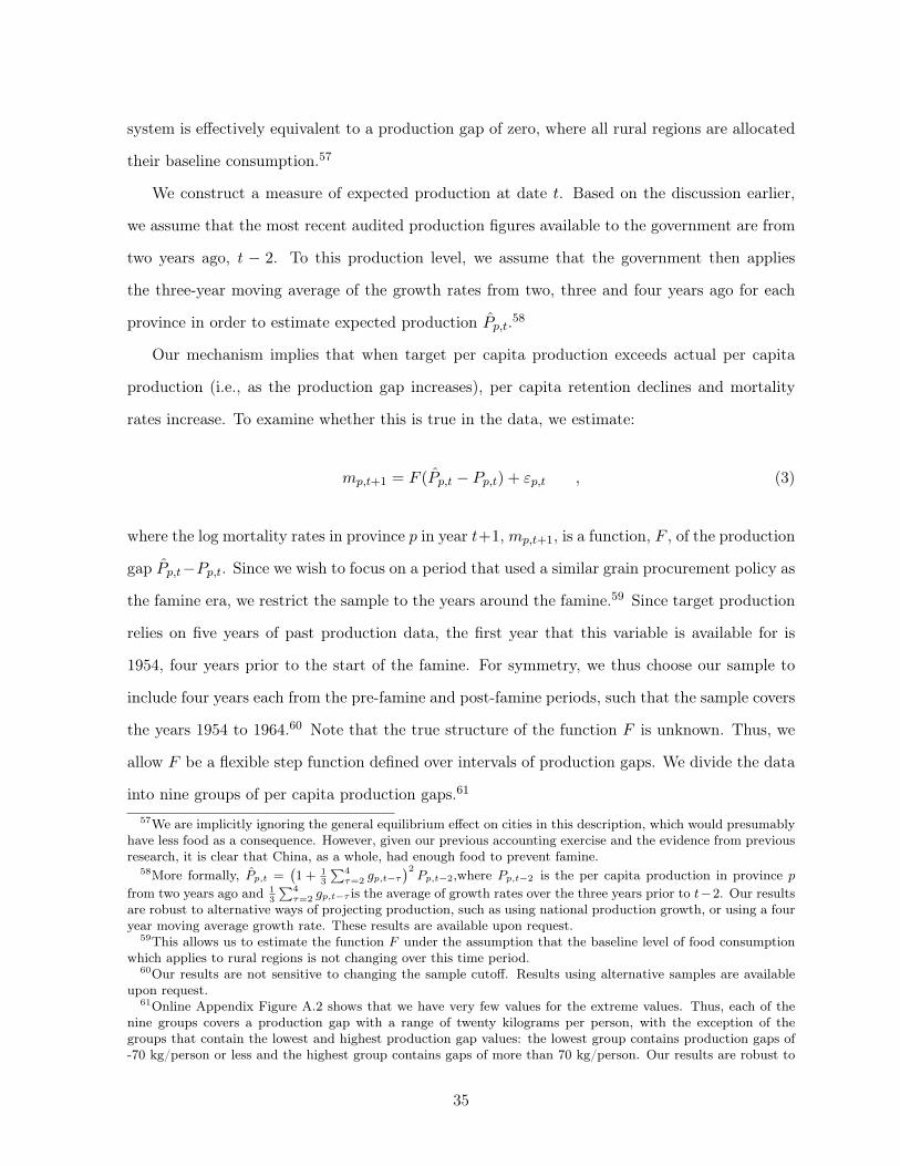
system is effectively equivalent to a production gap of zero, where all rural regions are allocated

their baseline consumption.57

We construct a measure of expected production at date t. Based on the discussion earlier,

we assume that the most recent audited production figures available to the government are from

two years ago, t − 2. To this production level, we assume that the government then applies

the three-year moving average of the growth rates from two, three and four years ago for each

province in order to estimate expected production P̂p,t.58

Our mechanism implies that when target per capita production exceeds actual per capita

production (i.e., as the production gap increases), per capita retention declines and mortality

rates increase. To examine whether this is true in the data, we estimate:

mp,t+1 = F (P̂p,t − Pp,t) + εp,t , (3)

where the log mortality rates in province p in year t+1, mp,t+1, is a function, F , of the production

gap P̂p,t−Pp,t. Since we wish to focus on a period that used a similar grain procurement policy as

the famine era, we restrict the sample to the years around the famine.59 Since target production

relies on five years of past production data, the first year that this variable is available for is

1954, four years prior to the start of the famine. For symmetry, we thus choose our sample to

include four years each from the pre-famine and post-famine periods, such that the sample covers

the years 1954 to 1964.60 Note that the true structure of the function F is unknown. Thus, we

allow F be a flexible step function defined over intervals of production gaps. We divide the data

into nine groups of per capita production gaps.61

57We are implicitly ignoring the general equilibrium effect on cities in this description, which would presumablyhave less food as a consequence. However, given our previous accounting exercise and the evidence from previousresearch, it is clear that China, as a whole, had enough food to prevent famine.

58More formally, P̂p,t =(1 + 1

3

∑4τ=2 gp,t−τ

)2Pp,t−2,where Pp,t−2 is the per capita production in province p

from two years ago and 13

∑4τ=2 gp,t−τ is the average of growth rates over the three years prior to t−2. Our results

are robust to alternative ways of projecting production, such as using national production growth, or using a fouryear moving average growth rate. These results are available upon request.

59This allows us to estimate the function F under the assumption that the baseline level of food consumptionwhich applies to rural regions is not changing over this time period.

60Our results are not sensitive to changing the sample cutoff. Results using alternative samples are availableupon request.

61Online Appendix Figure A.2 shows that we have very few values for the extreme values. Thus, each of thenine groups covers a production gap with a range of twenty kilograms per person, with the exception of thegroups that contain the lowest and highest production gap values: the lowest group contains production gaps of-70 kg/person or less and the highest group contains gaps of more than 70 kg/person. Our results are robust to

35

First, we test our main prediction that mortality was positively correlated with the production

gap by regressing mortality rates on the nine production gap interval dummy variables. The

coefficients and standard errors are shown in Table 6 column (1). The coefficients are also plotted

in Figure 6a. The finding that the coefficients are positive and nearly identical in size for the five

lowest groups, where the gaps are negative or zero (e.g., realized production equals or exceeds

target production), but increase for the groups with positive gaps (e.g., realized production is

below target production) is consistent with the fact that death can occur for many reasons (e.g.,

natural causes), but will increase further when the gap is positive. In other words, a positive

production gap leads to “excess” mortality. The fact that the coefficients are roughly increasing

with the magnitude of the production gaps when the gap is positive is consistent with higher

gaps leading to more mortality (i.e., our hypothesis).

At the bottom of the table, we present p-values for whether the coefficients for the negative

gap groups (the four lowest gap groups) or the positive gap groups (the four highest gap groups)

are jointly different from the fifth group (the group that contains zero-value production gaps).

The estimates show that the coefficients for all of the groups with negative or zero values of pro-

duction gaps are statistically similar, but the coefficients for the groups with positive production

gaps are statistically different from the group that contains zero production gaps.

To verify that this pattern is not confounded by the influences of GLF intensity, we add the

first principal component of the GLF as a control. Note that the sample size is reduced because

we do not have GLF variables for all provinces. However, the estimates shown in Table 6 column

(2) are almost identical to those in column (1).62

Second, we investigate whether the positive correlation between mortality and the production

gap is unique to the famine years, or if it is more generally a feature of the inflexible procurement

system, as is implied by our model. To this end, we repeat the exercise from column (1) on a

sample that excludes the three famine years. The estimates are shown in column (3) of Table 6.

The fitted values from these estimates are plotted with those from the full sample estimates from

using more or fewer intervals as long as there are sufficient observations per interval. Our results are also similarif, for symmetry, we restrict the sample to exclude observations with production gaps of more than 100 kg/personor less than -100 kg/person. Similarly, they are unchanged if we use alternative specifications that replace the stepfunction with a polynomial function. These results are not presented for brevity and are available upon request.

62The results are similar if we add controls for each individual GLF proxy instead of the first principal compo-nent. When we do this, the total contribution of the production gap to famine mortality increases to 47%.

36

column (1) in Figure 6b. They look very similar, which means that indeed, the cross-sectional

patterns during the famine are similar to those outside of the famine.

Third, we examine the implication of the model that a production gap of zero, which would

result from a fully flexible procurement policy, leads to much less famine mortality. This is

obviously true when we apply the regression estimates from Table 6 column (1). The coefficient

for the production gap group that contains the zero value (e.g., Group 5: -10 to 10 kg/person) is

11.13, which is nearly identical to the 10.66 average in the data for the three years right before

the famine (see Figure 1a).63 Thus, our empirical results are consistent with the prediction that

a fully flexible procurement policy would not have generated excess mortality during the famine.

Finally, we attempt to provide a crude quantification of the aggregate impact of our mecha-

nism for the famine. The benchmark total mortality in China in a given year is estimated as the

mortality rate under a production gap of zero (the coefficient for the fifth gap group in Table

6) multiplied by the total population across all of the provinces in our sample. Predicted total

mortality from the model in a given year is the sum of the predicted mortality across provinces.

For each province, this is the product of the predicted mortality rates under that province’s

production gap that year and the province’s population that year. Predicted excess mortality is

therefore the difference between the model predicted total mortality and the benchmark total

mortality for the three years of famine 1959-1961. Reported excess mortality is the difference

between the reported total mortality (the sum of all mortality across provinces in reported in

the data) and the benchmark total mortality for 1959-1961. To assess the contribution of the

hypothesized procurement policy to total excess mortality generated by the famine, we divide

the predicted excess famine mortality by the reported excess mortality.

Based on the model presented in column (1), this is 43%. If we use the model in column

(2) that controls for GLF intensity, the contribution of the inflexible procurement policy is 45%.

When we apply the estimates from column (3) that is the same regression model as in column

(1) but only use data from non-famine years to the production gaps during the famine, we

find that production gaps explain 39.5% of famine mortality. These “out-of-sample” predictions

provide strong evidence for our procurement hypothesis by showing that the quantitative impor-63The results are similar if we define the zero value production gap group with narrower or wider intervals

around zero. They are available upon request.

37

tance of production gaps for explaining famine mortality does not rely on underlying structural

relationships unique to the famine.

In summary, the results show that our proposed procurement policy contributed to 40 to 45%

of famine mortality, and was quantitatively important.64

These estimates also illustrate the importance of progressiveness. Consider the estimated

mortality in a counterfactual scenario in which all provinces are subject to the average production

gap for the famine period, 14.9 kg/person.65 Since procurement was in practice proportional to

the production gap, this counterfactual scenario results in slightly less procurement from the

more productive regions and slightly more from the less productive regions, making the system

less progressive. Applied to the regression estimates in column (1), this leads to a mortality rate

of 10.42 per thousand people (see the coefficient for the sixth group, which covers production

gaps that range from 10 to 30 kg/person). This is statistically similar to the mortality rate when

there is no production gap (e.g., the coefficient for the fifth production gap group).66 Therefore,

the progressiveness of the procurement system is crucial for the large quantitative effect of the

system’s inflexibility.67

6.3.2 Regional Procurement

We have thus far assumed that the positive association between the food production and mortality

rates are driven by procurement. In this section, we provide evidence for this mechanism by using

historical procurement data to test whether procurement rates increased more in more productive

regions during the famine.

We use regional procurement data from the famine era, which are available for the years

1953-82. The procurement data report the gross procurement and the amount that is “sold64Note that the fact that the contribution of our mechanism increases when we control for GLF factors is

consistent with the fact that the intensity of enforcement of some GLF policies were negatively correlated withgrain productivity.

65The calculation of the national average per capita production gap is similar to the procedure we describedfor calculating the per capita production gap for each province, except that we replace lagged province-specificproduction and growth rates with lags of aggregate production and growth rates.

66This result is not sensitive to the definition of the intervals. We obtain similar results (e.g., the mortalityrate of the counterfactual scenario is similar to the mortality rate when there is no production gap) when usingslightly wider or narrower intervals around 14.9. These results are available upon request.

67This exercise is equivalent to treating rural regions together as a single entity, which is in the spirit of theaccounting exercise of Section 3. Our result here are consistent with those of the accounting exercise which suggestthat inequality in food consumption across rural regions was necessary for the famine.

38

back” to provinces. The latter category includes food given back to rural areas for production

the following year (e.g., organic fertilizer, seeds) as well as food given back in the event of a

verified shock to production. We use these two measures to calculate net procurement. We then

calculate the procurement rate as the ratio of net procurement to production.

As with government-reported production data, we are concerned that the government un-

derreports famine-era procurement in order to minimize its responsibility for the famine. In

particular, we are concerned that for the famine years, the government would underreport pro-

curement more for regions that were more productive and suffered higher mortality rates. Unlike

the production data, we do not have a way for correcting for such measurement error. For these

reasons, we do not use the procurement data for the main quantification exercise and the in-

terpretation of the results below should be made with the caveat that that government-driven

non-random measurement error will likely attenuate the relative increase in procurement rate in

more productive regions.

We estimate equation (2) with the percentage of production procured as the dependent vari-

able. Figure 7 plots the coefficients and the 95% confidence intervals.68 Consistent with the

progressiveness of our hypothesized procurement policy, the estimated interaction coefficients

are positive for all years. This implies that procurement rates are always higher in more pro-

ductive regions.69 More importantly, the interaction terms increase in magnitude for the famine

years, which means that procurement rates during the famine increased more for productive re-

gions. The estimates are very precise. For the reasons discussed earlier, we do not interpret the

magnitudes of the estimates. However, the relative procurement rates across regions and their

changes over time are both consistent with our hypothesis.68The coefficients and standard errors are presented in Online Appendix Table A.4.69To see that procurement rates are always higher in the more productive regions under our hypothesis, see

Table 5. Procurement rates in Region A and B during a the high production year are 106/250 = 0.42 and29/170 = 0.17. During the low production year, they are 106/200 = 0.53 and 29/136 = 0.21. The differencebetween the two regions during the high production and low production years are thus 0.42 − 0.17 = 0.25 and0.53− 0.21 = 0.31.

39

7 Conclusion

During the twentieth century, millions have perished from famine, and sixty percent of total

famine mortality has occurred in centrally-planned economies. The most deadly famine in history

was the Chinese Great Famine, which in just a few years, killed approximately thirty million

individuals. This paper proposes that inflexible and progressive government procurement policy

is necessary for explaining the famine because other explanations cannot be easily reconciled with

the patterns of rural inequality in famine that we document, and rural inequality is necessary

to generate such a massive famine given high average rural food availability. Our results show

that the inflexible and progressive procurement policy contributed to 40-45% of total famine

mortality.

Our results do not mean that inflexible procurement must lead to famine. In the Chinese

context, inflexible procurement caused a famine because the government miscalculated grain

projections while aiming to procure an extremely large proportion of surplus production. Af-

ter the famine, perhaps with the realization that some degree of government miscalculation is

inevitable, the government lowered the procurement rate. As long as the government was com-

mitted to its inflexible procurement regime, lowering aggregate procurement goals was the only

policy instrument available for avoiding another famine.

The context of our study has many specific institutional features. However, the most essential

– the commitment to central planning, the incentives for regional bureaucrats and peasants to

misreport production, the incentives for peasants to shirk, the inability to quickly aggregate

and respond to new information – are common to most centrally planned economies of the

twentieth century. Therefore, our results can potentially provide insight into the famines that

have occurred in these other contexts. That there may be generalizable insights across these

fatal famines seems especially likely given the patterns of mortality and food production. For

example, for the Soviet Famine during 1932-33, which killed up to 6.5 million people in just one

year (Davies and Wheatcroft, 2004), there is a consensus that high government procurement

from rural areas caused the famine. Like the Chinese case, the most conservative estimates of

rural retention in the most severely stricken state, the Ukraine, show that average rural food

availability after procurement was deducted was approximately 170 kg/person during the worst

40

year of the famine (Conquest, 1987). While this amount, which provides a diet of approximately

1,671 calories per day, is not a rich diet, it is undeniably more than the level needed to avoid

mortality. Also, as in the case of China, the data suggest similar spatial patterns in mortality

rates – they are highest in the most productive regions.70

These provocative similarities suggest that the role of the inflexible procurement policy in

other historical famines like the Soviet Famine is a worthy topic of future research. In addition,

it is important to develop a more generalized framework for understanding the conditions under

which rigid food distribution mechanisms in centrally planned economies can cause famine. The

evidence offered in this study takes a first step in this agenda.70Conquest (1987) discusses the extremely high mortality rates in the states that produced the most food such

as the Ukraine and Kazakhstan. A recent study by Sharygin (2011) uses the RLMS data to construct regionalfamine mortality rates within Russia and finds that the agriculturally rich regions near the Volga suffered thehighest mortality rates.

41

References

Ashton, Basil, Kenneth Hill, Alan Piazza, and Robin Zeitz, “Famine in China, 1958-1961,” Population and Development Review, 1984, 10, 613–645.

Becker, Jasper, Hungry Ghosts: China’s Secret Famine., John Murray (Publishers) Ltd, 1996.

Burgess, Robin and Dave Donaldson, “Can Openness Mitigate the Effects of WeatherFluctuations? Evidence from India’s Famine Era,” 2010.

Cameron, A. Colin, Jonah B. Gelbach, and Douglas L. Miller, “Bootstrap-Based Im-provements for Inference with Clustered Errors,” The Review of Economics and Statistics,August 2008, 90 (3), 414–427.

Chang, Gene Hsin and Guanzhong James Wen, “Communal Dining and the ChineseFamine of 1958-1961,” Economic Development and Cultural Change, 1997, 46 (1), 1–34.

Conquest, R., The Harvest of Sorrow: Soviet Collectivization and the Terror-Famine ArmenianResearch Center Collection, Oxford University Press, Incorporated, 1987.

Dasgupta, Partha and Debraj Ray, “Inequality as a Determinant of Malnutrition and Un-employment: Theory,” The Economic Journal, 1986, 96 (384), 1011–1034.

Davies, R.W. and S.G. Wheatcroft, The Years of Hunger: Soviet Agriculture, 1931-1933The Industrialization of Soviet Russia, Palgrave Macmillan, 2004.

Dell, Melissa, Benjamin F. Jones, and Benjamin A. Olken, “Temperature Shocks andEconomic Growth: Evidence from the Last Half Century,” American Economic Journal:Macroeconomics, July 2012, 4 (3), 66–95.

Demick, Barbara, “The Good Cook: A Battle Against Famine in North Korea,” The NewYorker, 2009, November 2, 2009, 58–64.

Dikotter, Frank, Mao’s Great Famine: The History of China’s Most Devastating Catastrophe,1958-1962, Walker, 2010.

Dreze, Jean, The Economics of Famine, Vol. 101, Edward Elgar Publishing, 1999.

Eckstein, Alexander, China’s Economic Revolution, Cambridge University Press, 1977.

Fairbank, John King, Great Chinese Revolution 1800-1985 A Cornelia and Michael Bessiebook Volume 1442 of Perennial library, HarperCollins, 1987.

Haggard, Stephan and Marcus Noland, Hunger and Human Rights: the Politics of Faminein North Korea, Committee for Human Rights in North Korea, 2005.

Jia, Ruixue, “Weather Shocks, Sweet Potatoes and Peasant Revolts in Historical China,” HiC-NWorking Papers, 2011.

Johnson, D. Gale, “China’s Great Famine: Introductory Remarks,” China Economic Review,1998, 9 (2), 103–109.

42

Kinsella, K.G., H. Wan, and United States Bureau of the Census, An Aging World:2008 International Population Reports, U.S. Department of Commerce, Economics andStatistics Administration, U.S. Census Bureau, 2009.

Kung, James and Justin Yifu Lin, “The Causes of China’s Great Leap Famine, 1959-1961,”Economic Development and Cultural Change, October 2003, 52 (1), 51–73.

and Shuo Chen, “The Tragedy of the Nomenklatura: Career Incentives and PoliticalRadicalism during China’s Great Leap Famine,” American Political Science Review, 1 2011,105, 27–45.

Li, Wei and Dennis Tao Yang, “The Great Leap Forward: Anatomy of a Central PlanningDisaster,” Journal of Political Economy, 2005, 113 (4), 840–877.

Lin, Justin Yifu, “Collectivization and China’s Agricultural Crisis in 1959-1961,” Journal ofPolitical Economy, 1990, pp. 1228–1252.

and Dennis Tao Yang, “Food Availability, Entitlements and the Chinese Famine of1959-61,” Economic Journal, January 2000, 110 (460), 136–58.

Meng, Xin, Nancy Qian, and Pierre Yared, “The Institutional Causes of China- GreatFamine, 1959-1961,” NBER Working Paper No. 16361, 2010.

Nunn, Nathan and Nancy Qian, “Aiding Conflict: The Consequences of U.S. Food Aid onConflict,” Yale University Working paper, 2011.

and , “The Impact of Potatoes on Old World Population and Urbanization,” QuarterlyJournal of Economics, forthcoming.

OGrada, Cormac, “Making Famine History,” Journal of Economic Literature, 2007, 45 (1),5–38.

Oi, J.C., State and Peasant in Contemporary China: The Political Economy of Village Gov-ernment Center for Chinese Studies, UC Berkeley Series, University of California PressonDemand, 1991.

Peng, Xizhe, “Demographic Consequences of the Great Leap Forward in China’s Provinces,”Population and Development Review, 1987, pp. 639–670.

Perkins, Dwight H. and Shahid Yusuf, Rural Development in China, Baltimore: JohnsHopkins University, 1984.

Ravallion, Martin, “Famines and Economics,” Journal of Economic Literature, September1997, 35 (3), 1205–1242.

Sen, Amartya, Poverty and Famines: An Essay on Entitlement and Deprivation 1981.

Sharygin, Ethan, “Stunting and Selection Effects of Famine: A Case Study in Russia,” Uni-versity of Pennsylvania Working Paper, 2011.

Shiue, Carol H., “Transport Costs and the Geography of Arbitrage in Eighteenth-CenturyChina,” American Economic Review, 2002, pp. 1406–1419.

43

Spence, J.D., The Search for Modern China, W W Norton & Company Incorporated, 1990.

Thaxton, Ralph, Catastrophe and Contention in Rural China: Mao’s Great Leap ForwardFamine and the Origins of Righteous Resistance in Da Fo Village, New York: CambridgeUniversity Press, 2008.

tzu Sun, Wei, “Principles for Organizing Grain Circulation Planning,” Jihuajingji [PlannedEconomy in Chinese], 1958, 29, 24–7.

Walker, K.R., Planning in Chinese Agriculture: Socialisation and the Private Sector,1956-1962,Psychology Press, 1965.

, Food Grain Procurement and Consumption in China Contemporary China Institute Pub-lications, Cambridge University Press, 1984.

West, Loraine A. and Yaohui Zhao, Rural Labor Flows in China, Vol. 42, Univ of CaliforniaInst of East, 2000.

Yang, Dali, Calamity and Reform in China: State, Rural Society, and Institutional Changesince the Great Leap Famine, Stanford University Press, 1998.

Yao, Shujie, “A Note on the Causal Factors of China’s Famine in 1959-1961,” The Journal ofPolitical Economy, 1999, 107 (6), 1365–1369.

44

Tab

le1:

Average

Rural

Food

Availa

bility

Gra

in

Pro

d To

tal P

opR

ural

P

opN

at'l

Pro

c R

ate

(Mill

ions

To

ns)

(100

00

Per

sons

)(1

0000

P

erso

ns)

(Pro

c/P

rod)

(Kgs

/Yr)

(Cal

orie

s/D

ay)

(Kgs

)(C

alor

ies/

Day

)

Year

(1)

(2)

(3)

(4)

(5)

(6)

(7)

(8)

1957

133

4731

539

735

0.15

282

2767

285

2802

1958

142

4861

239

955

0.19

292

2867

289

2842

1959

123

4993

339

603

0.24

246

2421

237

2329

1960

106

4957

638

937

0.19

214

2101

221

2168

1961

101

4973

940

071

0.16

204

2005

212

2080

1962

115

5094

742

092

0.15

226

2223

234

2301

1963

123

5236

643

279

0.15

234

2303

242

2376

Per

Cap

ita R

ural

Ret

entio

nP

er C

apita

Pro

duct

ion

Notes: T

he s

ampl

e co

ntai

ns 1

9 pr

ovin

ces.

Sou

rces

: CD

SM

50 (1

999)

, CP

IRC

(200

0), t

he M

inis

try o

f Agr

icul

ture

(198

3) a

nd th

e au

thor

s'

com

puta

tions

.

45

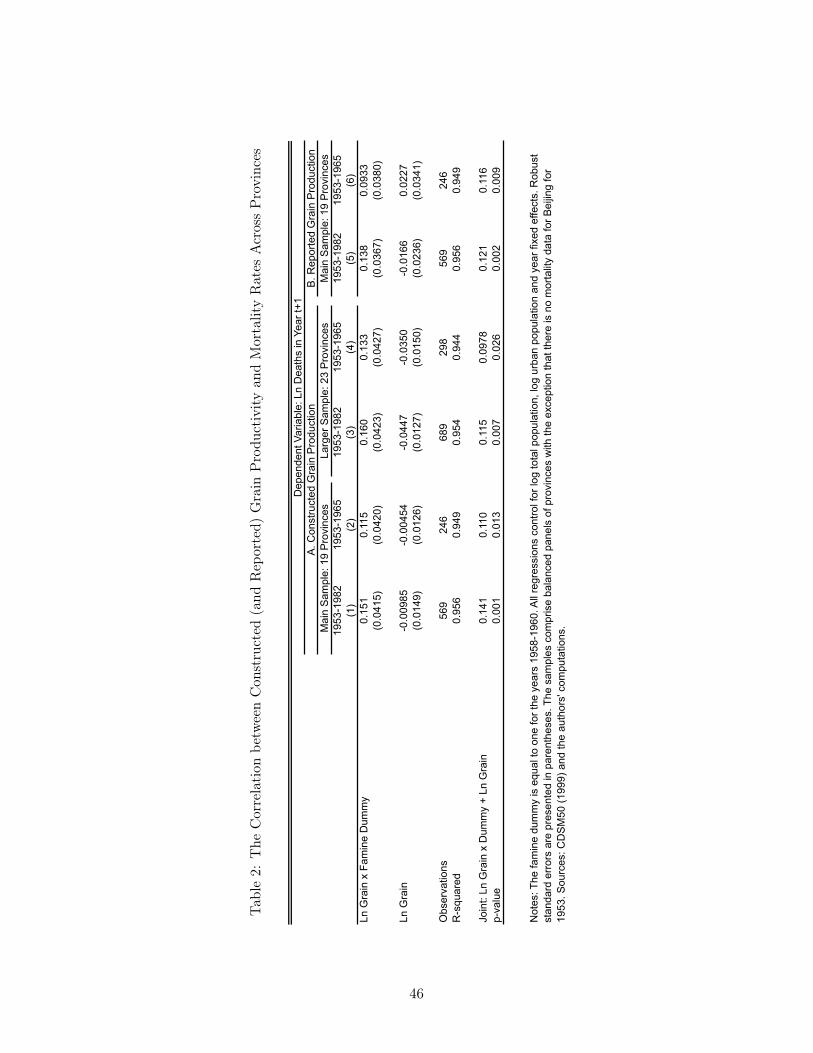
Tab

le2:

The

Correlation

betw

eenCon

structed

(and

Rep

orted)

Grain

Produ

ctivityan

dMortalityRates

AcrossProvinc

es

1953

-198

219

53-1

965

1953

-198

219

53-1

965

1953

-198

219

53-1

965

(1)

(2)

(3)

(4)

(5)

(6)

Ln G

rain

x F

amin

e D

umm

y0.

151

0.11

50.

160

0.13

30.

138

0.09

33(0

.041

5)(0

.042

0)(0

.042

3)(0

.042

7)(0

.036

7)(0

.038

0)

Ln G

rain

-0.0

0985

-0.0

0454

-0.0

447

-0.0

350

-0.0

166

0.02

27(0

.014

9)(0

.012

6)(0

.012

7)(0

.015

0)(0

.023

6)(0

.034

1)

Obs

erva

tions

569

246

689

298

569

246

R-s

quar

ed0.

956

0.94

90.

954

0.94

40.

956

0.94

9

Join

t: Ln

Gra

in x

Dum

my

+ Ln

Gra

in0.

141

0.11

00.

115

0.09

780.

121

0.11

6p-

valu

e0.

001

0.01

30.

007

0.02

60.

002

0.00

9

Dep

ende

nt V

aria

ble:

Ln

Dea

ths

in Y

ear t

+1

Not

es: T

he fa

min

e du

mm

y is

equ

al to

one

for t

he y

ears

195

8-19

60. A

ll re

gres

sion

s co

ntro

l for

log

tota

l pop

ulat

ion,

log

urba

n po

pula

tion

and

year

fixe

d ef

fect

s. R

obus

t st

anda

rd e

rror

s ar

e pr

esen

ted

in p

aren

thes

es. T

he s

ampl

es c

ompr

ise

bala

nced

pan

els

of p

rovi

nces

with

the

exce

ptio

n th

at th

ere

is n

o m

orta

lity

data

for B

eijin

g fo

r 19

53. S

ourc

es: C

DS

M50

(199

9) a

nd th

e au

thor

s' c

ompu

tatio

ns.

B. R

epor

ted

Gra

in P

rodu

ctio

nA

. Con

stru

cted

Gra

in P

rodu

ctio

nM

ain

Sam

ple:

19

Pro

vinc

esLa

rger

Sam

ple:

23

Pro

vinc

esM

ain

Sam

ple:

19

Pro

vinc

es

46

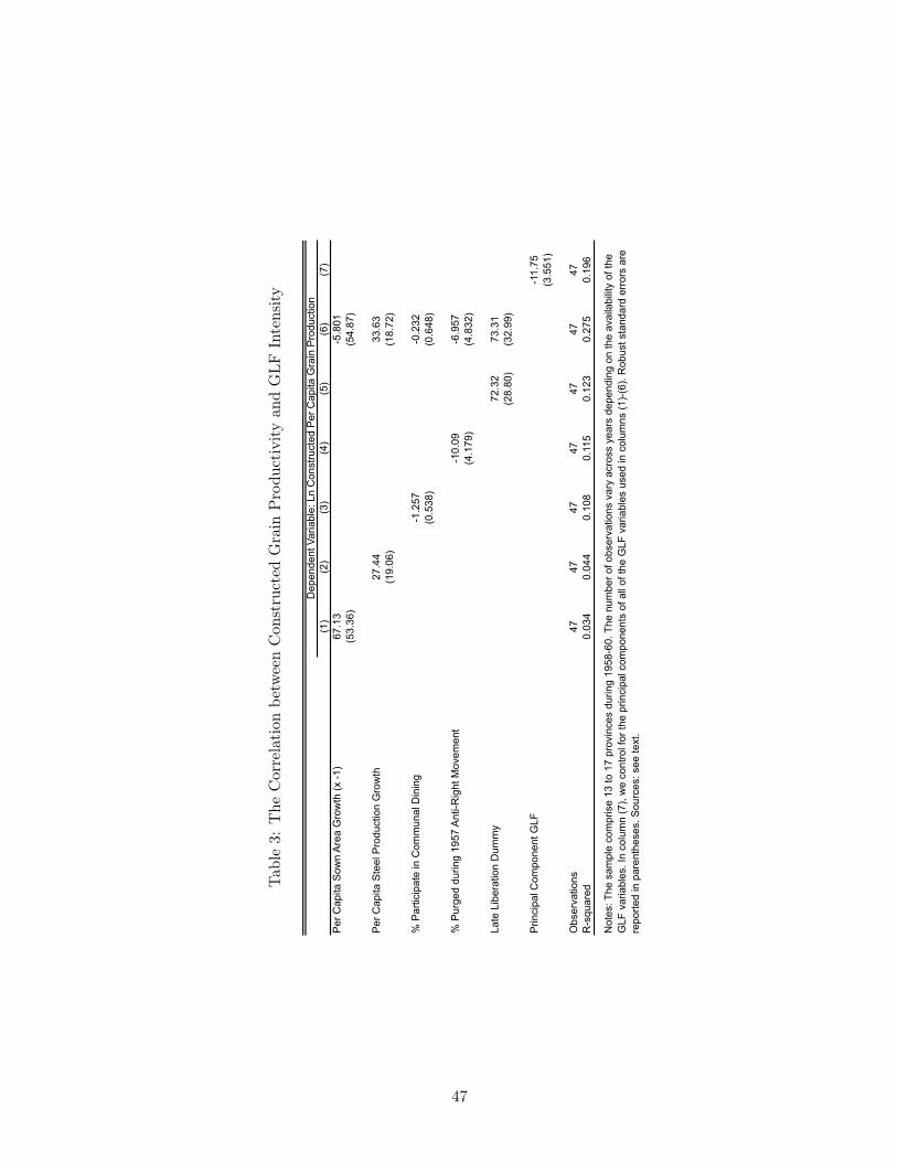
Tab

le3:

The

Correlation

betw

eenCon

structed

Grain

Produ

ctivityan

dGLF

Intensity

(1)

(2)

(3)

(4)

(5)

(6)

(7)

Per

Cap

ita S

own

Are

a G

row

th (x

-1)

67.1

3-5

.801

(53.

36)

(54.

87)

Per

Cap

ita S

teel

Pro

duct

ion

Gro

wth

27.4

433

.63

(19.

06)

(18.

72)

% P

artic

ipat

e in

Com

mun

al D

inin

g-1

.257

-0.2

32(0

.538

)(0

.648

)

% P

urge

d du

ring

1957

Ant

i-Rig

ht M

ovem

ent

-10.

09-6

.957

(4.1

79)

(4.8

32)

Late

Lib

erat

ion

Dum

my

72.3

273

.31

(28.

80)

(32.

99)

Prin

cipa

l Com

pone

nt G

LF-1

1.75

(3.5

51)

Obs

erva

tions

4747

4747

4747

47R

-squ

ared

0.03

40.

044

0.10

80.

115

0.12

30.

275

0.19

6

Not

es: T

he s

ampl

e co

mpr

ise

13 to

17

prov

ince

s du

ring

1958

-60.

The

num

ber o

f obs

erva

tions

var

y ac

ross

yea

rs d

epen

ding

on

the

avai

labi

lity

of th

e G

LF v

aria

bles

. In

colu

mn

(7),

we

cont

rol f

or th

e pr

inci

pal c

ompo

nent

s of

all

of th

e G

LF v

aria

bles

use

d in

col

umns

(1)-

(6).

Rob

ust s

tand

ard

erro

rs a

re

repo

rted

in p

aren

thes

es. S

ourc

es: s

ee te

xt.

Dep

ende

nt V

aria

ble:

Ln

Con

stru

cted

Per

Cap

ita G

rain

Pro

duct

ion

47

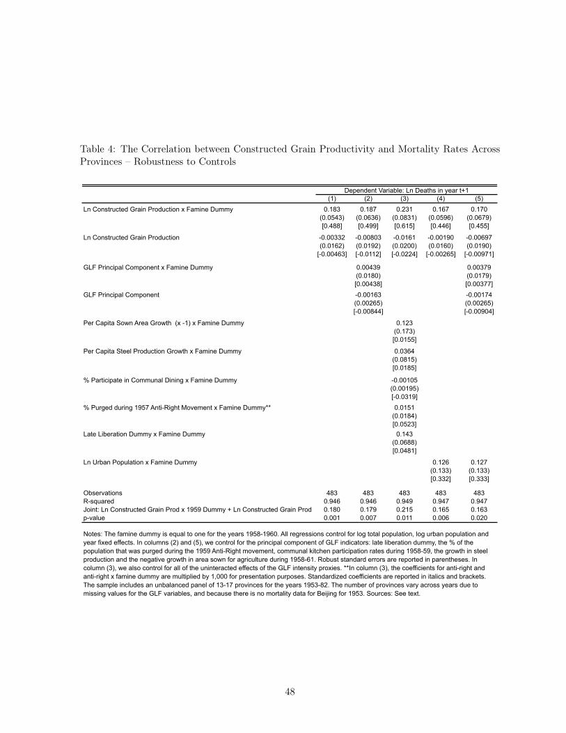
Table 4: The Correlation between Constructed Grain Productivity and Mortality Rates AcrossProvinces – Robustness to Controls

(1) (2) (3) (4) (5)Ln Constructed Grain Production x Famine Dummy 0.183 0.187 0.231 0.167 0.170

(0.0543) (0.0636) (0.0831) (0.0596) (0.0679)[0.488] [0.499] [0.615] [0.446] [0.455]

Ln Constructed Grain Production -0.00332 -0.00803 -0.0161 -0.00190 -0.00697(0.0162) (0.0192) (0.0200) (0.0160) (0.0190)

[-0.00463] [-0.0112] [-0.0224] [-0.00265] [-0.00971]

GLF Principal Component x Famine Dummy 0.00439 0.00379(0.0180) (0.0179)[0.00438] [0.00377]

GLF Principal Component -0.00163 -0.00174(0.00265) (0.00265)[-0.00844] [-0.00904]

Per Capita Sown Area Growth (x -1) x Famine Dummy 0.123(0.173)[0.0155]

Per Capita Steel Production Growth x Famine Dummy 0.0364(0.0815)[0.0185]

% Participate in Communal Dining x Famine Dummy -0.00105(0.00195)[-0.0319]

% Purged during 1957 Anti-Right Movement x Famine Dummy** 0.0151(0.0184)[0.0523]

Late Liberation Dummy x Famine Dummy 0.143(0.0688)[0.0481]

Ln Urban Population x Famine Dummy 0.126 0.127(0.133) (0.133)[0.332] [0.333]

Observations 483 483 483 483 483R-squared 0.946 0.946 0.949 0.947 0.947Joint: Ln Constructed Grain Prod x 1959 Dummy + Ln Constructed Grain Prod 0.180 0.179 0.215 0.165 0.163p-value 0.001 0.007 0.011 0.006 0.020

Dependent Variable: Ln Deaths in year t+1

Notes: The famine dummy is equal to one for the years 1958-1960. All regressions control for log total population, log urban population and year fixed effects. In columns (2) and (5), we control for the principal component of GLF indicators: late liberation dummy, the % of the population that was purged during the 1959 Anti-Right movement, communal kitchen participation rates during 1958-59, the growth in steel production and the negative growth in area sown for agriculture during 1958-61. Robust standard errors are reported in parentheses. In column (3), we also control for all of the uninteracted effects of the GLF intensity proxies. **In column (3), the coefficients for anti-right and anti-right x famine dummy are multiplied by 1,000 for presentation purposes. Standardized coefficients are reported in italics and brackets. The sample includes an unbalanced panel of 13-17 provinces for the years 1953-82. The number of provinces vary across years due to missing values for the GLF variables, and because there is no mortality data for Beijing for 1953. Sources: See text.

48

Table 5: A Stylized Example of Grain Procurement

Region A Region B City

Subsistence Needs 100 100 100

Production under High Shock (Probability 80%) 250 170 0

Production under Low Shock (Probability 20%) 200 136 0

Expected Production (0.8 x High + 0.2 x Low) 240 163 0

Expected Consumption 134 134 134

Procurement/Subsidy (Expected Production - Expected Consumption) 106 29 -134

Consumption under High Shock (High Production - Procurement) 144 141 134

Consumption under Low Shock (Low Production - Procurement) 94 107 134Sources: Author's calculations.

49

Tab

le6:

The

Correlation

betw

eentheProdu

ctionGap

andMortalityRates

(1)

(2)

(3)

1954

-196

419

54-1

964

1954

-195

7, 1

961-

1964

Gov

ernm

ent P

roje

cted

PC

Pro

d - R

ealiz

ed P

C P

rod

is

Gro

up1:

<=-

7011

.30

11.2

610

.66

(0.6

04)

(0.5

83)

(0.6

05)

G

roup

2: (-

70, -

50]

10.0

010

.00

10.0

0(0

.372

)(0

.377

)(0

.377

)

Gro

up3:

(-50

,-30]

11.6

211

.59

10.4

2(0

.555

)(0

.553

)(0

.395

)

G

roup

4: (-

30, -

10]

10.4

310

.65

9.93

1(0

.648

)(0

.647

)(0

.552

)

Gro

up5:

(-10

, 10]

11.1

311

.75

9.43

8(0

.897

)(1

.008

)(0

.393

)

Gro

up6:

(10,

30]

10.4

210

.59

10.1

8(0

.336

)(0

.355

)(0

.310

)

G

roup

7: (3

0, 5

0]14

.87

14.8

810

.38

(3.0

72)

(3.0

93)

(0.6

15)

G

roup

8: (5

0, 7

0]12

.85

12.8

810

.97

(1.0

41)

(1.0

64)

(0.6

81)

G

roup

9: >

7012

.00

12.1

511

.82

(0.5

96)

(0.6

04)

(0.6

69)

Con

trols

GLF

PC

AN

YN

Obs

erva

tions

185

175

129

R-s

quar

ed0.

819

0.81

70.

968

Diff

eren

t to

Gro

up5

(p-v

alue

) G

roup

s 1,

2,3,

40.

113

0.09

770.

366

Gro

ups

6,7,

8,9

0.03

550.

0484

0.03

16

Dep

ende

nt V

aria

ble:

Ln

Dea

thra

te in

Yea

r t+1

Not

es: R

obus

t sta

ndar

d er

rors

are

in p

aren

thes

es.T

he p

-val

ues

at th

e bo

ttom

of t

he ta

ble

test

the

join

t diff

eren

ce to

the

Gro

up5

coef

ficie

nt. T

he c

ontro

l for

GLF

is th

e fir

st p

rinci

pal c

ompo

nent

of G

LF in

dica

tors

: lat

e lib

erat

ion

dum

my,

the

% o

f pop

ulat

ion

in th

e C

omm

unis

t Par

ty in

the

late

195

0s, t

he n

umbe

r of i

ndiv

idua

ls p

urge

d du

ring

the

1957

Ant

i-Rig

ht m

ovem

ent,

com

mun

al k

itche

n pa

rtici

patio

n ra

tes

durin

g 19

58-5

9, th

e gr

owth

in s

teel

pro

duct

ion,

the

grow

th in

agr

icul

tura

l pop

ulat

ion

and

the

grow

th in

are

a so

wn

for a

gric

ultu

re d

urin

g 19

58-6

1. S

ourc

es: C

DS

M50

(199

9) a

nd th

e au

thor

s' c

ompu

tatio

ns.

50

Figure 1: Average and Spatial Variation in Famine Severity

(a) Province-level Mortality Rates – Mean and Cross-Province Standard Deviation

0.2

.4.6

.8C

ross-P

rovin

ce

SD

/Me

an

51

01

52

0D

ea

ths p

er

1,0

00

1950 1960 1970 1980 1990 2000Year

Mean Mortality Rates Cross-Province SD/Mean

(b) County-level Survivor Birth Cohort Sizes – Mean

40

50

60

70

80

90

Co

ho

rt S

ize

1%

1950 1955 1960 1965Year (Birth Year)

(c) County-level Survivor Birth Cohort Sizes – De-trended Mean and Cross-County Standard Deviation

.2.2

5.3

.35

.4C

ross-C

ou

nty

Std

De

v /

Me

an

.6.8

11

.21

.4C

oh

ort

Siz

e /

Avg

Co

un

ty C

oh

ort

Siz

e

1950 1955 1960 1965Year(Birth Year)

Cohort Size Ratio Cross-County Std Dev / Mean

51

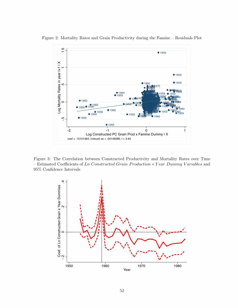
Figure 2: Mortality Rates and Grain Productivity during the Famine – Residuals Plot

1958

1959

1960

1958

1959

1960

1958

1959

1960

19591960

1958

1959

1958

1958

1960

1958

195919591960

1960

1979

1954

1960

1955

1955195719561954

1954

1955

195619571982

197619561975197719691957

1981197119811980197419721978197919691974

1964

198019731975

1970

19671972

1966196819821976

1953

197619671978197119541980

1953

19811982

1962

196319781974197319661977

1965

1959

1965197919771968

197319711956

1962197919721963196119641961

19751956

1954

1955

197019671966195719541962

19551957195319691955

1961

1955

196519621978

1964196519741957

1963

19751969

19701966

1982197319561980

198019811982197219571964

19611954

1971196819761956

1955

1968

1981

19671955

19541974

1953

1973197219751979

1977

19761971

1954

195719781967

1977

1970

19571961

1953

1974

1956

196219611956

1963

1957

1956

196519811977

1955

1964196819661971198019621972

19611970

19761969

1962

1954

197519651970

1963

19811964

1964

1963

1978

1953

196919731968

1970

19821973

1975

197619741978

1982

1982

19631979

1977

1967

1981

1966

1965

19661969

1974

1979

1980

1972

1976

1980

1953

197119671962

1978

1968196819611970

19751977196719721973

1979

1971

1969197019661965

1962

196519631964

1968

19631961

19661970

19811973

1967

19681953

197219721980

1971

197719691973

1980

19751978197519741971

197819761982

197419701982

1975

19791969

1976

196619741977

1976

1953

1963

198019641978

19711965

19811968

197219771967

1966

19611958

1973

1967

1982

1964

1979197919811969

1964

1963

1957

196519531962

1962

1961

195419561955

19821978197619741977

19801979

1970197319721971

1954

1969195619671981195719611964195519751965

1953

19631953196819621966

1955

1963

19551954

1968197519781954

198119571980

1967

196219551956

19701971

19691973197719731974

19791982

1974

1956

1965

195419771976197219721976

1964

19811975195719781970

1965

1966

1964

1968

1966

1961

1961

1979

1956

19711972

1980198119821962

1963

1969196019571982

195319771956197719801973

1967

1961

197519661976

1970

197919781974

1976

1964

195319701968198119821979

19531971

1980197419711978

1975

1965

19681969

1969

1967

1963

1966

1967

19731957

19721955

19631954

1962

1964

19621965

1961

19621961

1963

19641965195319661959196719681969195419701971

19551957

197219731975

1956

197719761978198119801982

1953

1979

1974

19631964

19621965196119541955

1966

19571967

1968

19561969

196319621964

1970

1965

1961

19711974197219731975

1966

19771968

196719691978197619821981

1953

1980

1970

1979

1971

1960

19721974

1975

1973

19771976197819811982

19801979

1958

19571956

1959

1959

1955195419581960

19601958

19591958

1960

1959

1959

1958

1960

195819601960

1960

1958

1958

1958

1959

1960

1958

1959

1958

1959

1959

1959

1960

-.5

0.5

11

.5L

og

Mo

rta

lity R

ate

s in

ye

ar

t+1

| X

-2 -1 0 1Log Constructed PC Grain Prod x Famine Dummy | X

coef = .15101364, (robust) se = .04149286, t = 3.64

Figure 3: The Correlation between Constructed Productivity and Mortality Rates over Time– Estimated Coefficients of Ln Constructed Grain Production×Y ear Dummy V ariables and95% Confidence Intervals

-.2

0.2

.4

Co

ef.

of

Ln

Co

nstr

ucte

d G

rain

x Y

ea

r D

um

mie

s

1950 1960 1970 1980

Year

52

Figure 4: The Correlation between Geo-Climatic Conditions and Survivor Birth Cohort Size overTime

(a) Estimated Coefficients ofLn Mean Spring Temperature ×Y ear Dummy V ariables and 95% ConfidenceIntervals

-2-1

01

2C

oe

f. o

f L

n S

prin

g T

em

p x

Ye

ar

Du

mm

ies

1950 1955 1960 1965Year

(b) Estimated Coefficients ofLn Mean Spring Rainfall×Y ear Dummy V ariablesand 95% Confidence Intervals

-.3

-.2

-.1

0.1

.2C

oe

f. o

f L

n S

prin

g R

ain

x Y

ea

r D

um

mie

s

1950 1955 1960 1965Year

(c) Estimated Coefficients of Suitability Index ×Y ear Dummy V ariables and 95% Confidence Intervals

-.6

-.4

-.2

0.2

.4C

oe

f. o

f S

uita

bili

ty x

Ye

ar

Du

mm

ies

1950 1955 1960 1965Year

53

Figure 5: The Correlation between Constructed Productivity and Past Constructed Productivity

(a) 1958 vs. 1957 Productivity

10

02

00

30

04

00

50

06

00

19

58

Co

nstr

ucte

d P

er

Ca

pita

Pro

du

ctio

n -

- K

g/P

ers

on

100 200 300 400 500 6001957 Constructed Per Capita Production -- Kg/Person

(b) 1959 vs. 1958 Productivity

10

02

00

30

04

00

50

01

95

9 C

on

str

ucte

d P

er

Ca

pita

Pro

du

ctio

n -

- K

g/P

ers

on

100 200 300 400 500 6001958 Constructed Per Capita Production -- Kg/Person

(c) 1960 vs. 1959 Productivity

10

02

00

30

04

00

50

01

96

0 C

on

str

ucte

d P

er

Ca

pita

Pro

du

ctio

n -

- K

g/P

ers

on

100 200 300 400 5001959 Constructed Per Capita Production -- Kg/Person

(d) 1958 Productivity Growth vs. 1957 Productivity-.

4-.

20

.2.4

Gro

wth

Ra

te 1

95

7-5

8 C

on

str

ucte

d P

C P

rod

-200 0 200 400Constructed PC Prod in 1957

coef = -.00024323, se = .00039858, t = -.61

(e) 1959 Productivity Growth vs. 1958 Productivity

-.4

-.2

0.2

.4G

row

th R

ate

19

58

-59

Co

nstr

ucte

d P

C P

rod

-200 -100 0 100 200 300Constructed PC Prod in 1958

coef = -.00059098, se = .00029428, t = -2.01

(f) 1960 Productivity Growth vs. 1959 Productivity

-.2

-.1

0.1

.2.3

Gro

wth

Ra

te 1

95

9-6

0 C

on

str

ucte

d P

C P

rod

-100 0 100 200Constructed PC Prod in 1959

coef = -.00007669, se = .00028725, t = -.27

54

Figure 6: The Correlation between the Per Capita Production Gap and Mortality Rates

(a) Predicted Mortality Rates (Full Sample)

10

11

12

13

14

15

Pre

dic

ted

Ln

Mo

rta

lity R

ate

s in

Ye

ar

t+1

-100 0 100 200 300 400Gov Proj Prod PC - Realized Prod PC (kgs/person)

(b) Predicted Mortality Rates (Exclude the Three Years of Famine)

81

01

21

41

6P

red

icte

d L

n M

ort

alit

y R

ate

s in

Ye

ar

t+1

-100 0 100 200 300 400Gov Proj Prod PC - Realized Prod PC (kgs/person)

All Years Non-Famine Years

55

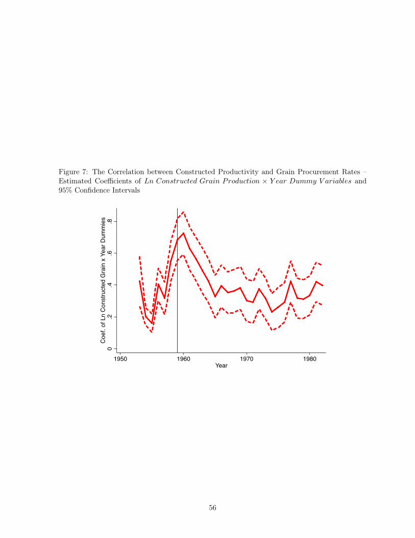
Figure 7: The Correlation between Constructed Productivity and Grain Procurement Rates –Estimated Coefficients of Ln Constructed Grain Production × Y ear Dummy V ariables and95% Confidence Intervals

0.2

.4.6

.8

Co

ef.

of

Ln

Co

nstr

ucte

d G

rain

x Y

ea

r D

um

mie

s

1950 1960 1970 1980

Year

56

ONLINE APPENDIX

A Production, Mortality and Procurement Data

Aggregate and provincial-level production, population, urban population and mortality data are

reported by the China Data and Statistical Materials for 50 Years, 1949-98 (CDSM50), which

is published by the National Statistics Bureau (NBS). Historical province-level demographic

breakdowns are published as tables from the 1953 Population Census, and made available to us

by the NBS. The typical concern for using production and mortality data reported by the Chinese

government is that it has historically under-reported mortality and over-reported production to

minimize the severity of the famine for political reasons. The data we use were published in

the post-Mao reform era and have been carefully corrected by the NBS to address potential

reporting errors from the Mao-years. The difficulty in such revisions results in missing data for

some provinces and some years (e.g., there is no data for Tibet until 1978, data for Sichuan are

missing for several years). Comparisons across data sources show that these demographic and

production data have been adjusted from the Mao-era reports (Ashton, Hill, Piazza and Zeitz,

1984). For example, the official figure for 1959 national grain production was 270 million tons

according to 1959 reports, but revised downwards to 200 million tons in the official reports in

1980, which was similar to the amount reported by the United States Department of Agriculture

and the U.S. Agriculture Attache in Hong Kong (Ashton, Hill, Piazza and Zeitz, 1984: Table 6).

The procurement data are reported by the Ministry of Agriculture in their publication, Nongye

Jingji Ziliao, 1949-1983. The data we use are the best that are available to researchers today

and have been used by recent studies such as Lin and Yang (2000), Li and Yang (2005) and

Kung and Chen (2011).

B Main Analysis Sample Restriction

In the 1950s, there were officially 24 provinces in total.71 These included three province-level

municipalities that were mostly urban, but still contained large fractions of agricultural pop-

ulations (Beijing, Shanghai and Tianjin). In addition, there were five regions that were given71The present day provinces of Chongqing and Hainan had not yet attained provincial status.

1

official political “autonomy” due to historical political reasons (Tibet, Xinjiang, Inner Mongolia,

Guangxi and Ningxia). Our main sample excludes the five officially autonomous regions because

they faced different political and economic policies. Amongst the 24 provinces, we exclude four

provinces with large ethnic minority populations that live in autonomous communities (Qing-

hai, Gansu, Yunnan and Guizhou) because these autonomous communities also faced different

political and economic policies, and Sichuan because there is no mortality data for this province

for 1958 and 1959. Thus, the main sample used in this paper uses 19 of the 24 provinces that

existed during the famine era.

The main insights that rural retention was, on average, enough to avoid a famine and that

famine severity was positively associated with food productivity are not unique to our chosen

sample. In Section 4.1, we show that our main results are similar when we use all 23 provinces

for which we have data. In an earlier version of the paper, we also show that our results are

similar when we include the autonomous regions, though they are less precisely estimated (Meng

et al., 2009). In addition, we also show that average rural food production in each province was

sufficient for survival in all of the provinces in our sample, and was sufficient for heavy adult

labor in all provinces except the municipalities, which suffered little famine mortality. The main

difference for the excluded provinces is that our projection of the government’s target production

(Section 6.3.1) is much noisier (we obtain many more extremely high values of production gaps),

which is consistent with the fact that the excluded regions faced different procurement policies.

C Weather Data

The weather data is reported by the Terrestrial Air Temperature and Precipitation: Monthly and

Annual Time Series (1950 - 1996) data set. Similar data has been used by Dell, Jones and Olken

(2012) and Nunn and Qian (2011b). The Chinese weather data were never meant to be publicly

released and therefore unlikely to have been manipulated by the famine-era government.72 We

use ArcGIS to calculate the monthly mean temperature and precipitation for each county for the

years 1950-66.72The data was made available only very recently for historical climatology studies. Detailed documentation is

provided at http://climate.geog.udel.edu/~climate/html_pages/README.ghcn_ts.html.

2

For the weather variables used in estimating the production function using province-level data

(Section 5.1), we calculate the sum of all rainfall and temperature in a province in each month.

For each year and province, we have twelve rainfall variables and twelve temperature variables.

We can alternatively use mean temperature or rainfall, or measure rainfall and temperature as

deviations from their historic means (for each province). This does not change the constructed

grain production estimates. Hence, we only report one specification for brevity. Results from

other specifications are available upon request. Note that weather stations do not cover all areas

in each province. This results in measurement error in independent variables. We can adjust

for this by calculating the area covered by weather stations in each province and adjusting

output proportionally (e.g., if weather stations cover 70% of a province, we adjust production

and population downwards by multiplying each variable by 0.7). This does not change the results

since we are interested in per capita production. These corrections are not reported for brevity.

For the weather variables used in the county-level estimates of the relationship between cohort

size and natural conditions (Section 5.3), we calculate the sum of all rainfall and temperature

in each county during spring months in a year. We construct one temperature and one rainfall

variable per county-year observation so that the coefficients of this reduced form regression are

easy to interpret. The focus on the spring months is motivated by studies of historical Chinese

agriculture, which argue that warm spring temperatures and plentiful precipitation were typically

the most important factors for a good grain harvest (Walker, 1965, 1984).

For the county-level analysis, we restrict our sample to the counties for that report historical

weather data. For the province-level analysis, we aggregate the data from these counties for each

province. Since we do not have weather data for every county in each province, this means that

the province-level weather data are measured with noise.

D Suitability Data

The measure of suitability for grain cultivation is constructed from a model and data provided

by the Food and Agriculture Organization’s GAEZ (2002) database. It is based purely on the

biophysical environment of a region and is not influenced by which crops are actually adopted in

an area. Factors that are easily affected by human actions, such as soil pH, are not parameters

3

in this model. The suitability measure at the county level is the fraction of grids within a county

that is suitable for the production of all types of grains that were produced in China during

the 1950s, a measure we use for the sake of computational ease. The suitability measure at

the province level is the fraction of grids within a province that is suitable for the same set

of crops. These data and similar measures have recently been used for the historical Chinese

context in Nunn and Qian (2011a, 2011b) and Jia (2011). See Nunn and Qian (2011a) for a

detailed discussion of the underlying parameters of the GAEZ model.

E Per Capita Caloric Requirements in 1953

The first benchmark of the caloric requirement for heavy adult labor and healthy child develop-

ment is constructed by combining data on caloric requirements by age and sex, as recommended

by the United States Department of Agriculture (USDA), with data on population, age and

sex distribution in China from the 1953 Population Census.73 The USDA recommends caloric

requirements according to the age and sex of an individual, and the degree of activity. For this

calculation, we use the caloric guidelines for the highest level of activity. Since the Census di-

vides individuals into broader age categories than the USDA guidelines, we calculate the average

caloric requirement for each sex-age group as the average recommended caloric requirements

across all of the ages in each group. It is important to note that the USDA recommendations

are extremely generous and approximately 20% higher than the average caloric consumption of

East Asian countries during the mid-1960s.74

The second benchmark of the caloric requirement for avoiding mortality is calculated to be

43% of the first benchmark due to the scant medical evidence on the amount of calories needed

to stay alive. Therefore, we follow Dasgupta and Ray’s (1986) assumption that 900 calories are

required for an adult male to do some work, and conservatively assume that a similar amount

is needed to stay alive. Since 900 calories is 43% of the USDA recommendations for heavy

labor by an adult male, we construct the benchmark calories for survival by assuming that the73USDA guidelines are published at http://www.cnpp.usda.gov/Publications/USDAFoodPatterns/EstimatedCalorieNeedsPerDayTable.pdf74Average per capita food consumption is reported for different time periods and regions by the Food and

Agriculture Organization (2002).

4

requirement is 43% of USDA recommendations for all age and sex groups.75

The estimation for average caloric requirements once the demographic breakdown is taken

into account is shown in Online Appendix Table A.1. We estimate that for China, as a whole,

1,871 calories were needed per person per day on average for heavy labor and normal child

development, and 804 calories were needed per person per day on average to stay alive in 1953.

Our accounting exercise assumes that the per capita requirements during the famine are similar

to 1953.

F Within-Province Variation in Famine Intensity

We construct a proxy for famine severity that is each county’s birth-cohort size when it was

lowest during the famine (1959-1960) relative to its non-famine cohort size (1954-1957). This

proxy takes a smaller value when the famine is more severe. For example, it is less than one if the

birth-cohort size of individuals born during the famine is smaller than that of individuals who

were age two to five years when the famine began. A value that is greater than one would suggest

that a county was relatively unaffected by the famine. Online Appendix Table A.2 columns (1)-

(4) present the estimated mean, normalized variance (standard deviation divided by the mean),

and the minimum and maximum values of this famine severity proxy for China as a whole and

for each province. These descriptive statistics show that for China as a whole, the famine birth-

cohort size is approximately 70% of the pre-famine birth-cohort size. However, there is enormous

spatial variation. For the hardest hit county, famine birth-cohort size was less than 14% of the

pre-famine cohort. Column (5) shows the fraction of counties within a province that suffered

relatively little famine, which we measure as the fraction of counties that have famine birth-cohort

sizes that are equal to or greater than pre-famine cohort sizes. Approximately 11% of counties

experienced little famine according to this measure. Note that the birth-cohort sizes of those

who were born during 1954-57 were also reduced by famine exposure. Thus, our proxy is likely75Note that our calculated thresholds are generally extremely generous and more than sufficiently take into

account additional calories needed for cold winter conditions. See an earlier version of this paper, Meng et al.(2010) for a discussion of the medical evidence. When comparing the caloric needs between our two benchmarks,one should also note that the relationship between calories consumed and work capacity is potentially highlynon-linear, as suggested by the nutritional poverty trap theory (Das Gupta and Ray, 1986). This does not playan important role for our study since production in 1959 was in excess of both benchmarks.

5

to understate the fraction of counties that suffered famine. The province-specific estimates show

that there is both substantial cross-province and within-province variation in famine severity.

The variation across provinces can be observed by comparing the famine birth-cohort size in the

hardest hit provinces of Anhui and Sichuan, which are nearly half as large as the pre-famine

birth-cohort size, to that of Beijing, where the famine and pre-famine cohort size are similar.

The variation within provinces can be observed from the large standard deviations of within-

province famine severity shown in column (2). We also investigate whether the spike in variance

is driven by outliers by plotting histograms of the county-level famine-to-non-famine birth-cohort

size ratio. They show that famine severity was distributed roughly normally across counties in

China, and across counties within each province. Thus, the observed variance in cross-county

and cross-province famine severity are not driven by outliers. The histograms are not presented

for brevity. Please see the previous version of the paper for these results.

G Reports of 1958 Production Falls

The political climate in 1959 was extremely tense and most likely caused leaders to follow rules,

even those that were likely to prove problematic later. The GLF had been received with cynicism

from many party officials from the very beginning, and its failures and successes were crucial

to Mao’s political leadership. In December 1958, at a meeting of the Central Committee of the

CCP in Wuhan, party leaders refused to fully endorse GLF policies. Following this meeting, Liu

Shaoqi replaced Mao, who remained Party Chairman, as the Head of State in early Spring of

1959 (Spence, 1990, pp.581). Many historians view this as an unwilling step down by Mao. It

is therefore not surprising that further challenges of the GLF resulted in a strong response from

Mao. In July 1959, Mao famously purged Peng Dehuai, a field marshal of exceptional political

standing, for criticizing collectivization and other GLF policies and expressing forebodings of

famine. These problems of the collective system mandated by the GLF were a source of con-

tention between communist party moderates and hard-liners who backed Mao. However, with

the exception of Peng Dehuai who did a tour of the countryside during the spring of 1959, there is

no evidence that any top leader ever obtained an accurate picture of the problems of collectiviza-

tion and the danger of famine. Peng reported these problems to Communist Party Chairman

6

Mao Zedong in a personal letter. The problems he mentioned included reduced incentives to

work, a diversion of labor away from agriculture, and over-procurement of grain by mid-level

party leaders who were under-pressure to fulfill grain target quotas that had been set too high.

Fearing a political revolt against his leadership based on perceived failures of the GLF, Mao used

the contents of this letter to purge Peng as a rightist at the historic Lushan conference in July

of 1959. At this conference, the top party leaders made clear that the first year of the GLF was

a success and that collectivization was increasing grain harvest more than ever (Becker, 1996, p.

87-92).

7

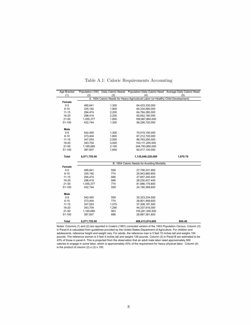
Table A.1: Caloric Requirements Accounting

Age Bracket Population (100) Daily Caloric Needs Population Daily Caloric Need Average Daily Caloric Need(1) (2) (3) (4) (5)

Female0-5 495,641 1,300 64,433,330,000

6-10 335,192 1,800 60,334,560,00011-15 294,474 2,200 64,784,280,00016-20 298,419 2,200 65,652,180,00021-50 1,055,377 1,800 189,967,860,00051-100 432,744 1,300 56,256,720,000

Male0-5 542,455 1,300 70,519,150,000

6-10 373,404 1,800 67,212,720,00011-15 347,053 2,500 86,763,250,00016-20 343,704 3,000 103,111,200,00021-50 1,165,685 2,100 244,793,850,00051-100 387,607 1,600 62,017,120,000

Total 6,071,755.00 1,135,846,220,000 1,870.70

Female0-5 495,641 559 27,706,331,900

6-10 335,192 774 25,943,860,80011-15 294,474 946 27,857,240,40016-20 298,419 946 28,230,437,40021-50 1,055,377 774 81,686,179,80051-100 432,744 559 24,190,389,600

Male0-5 542,455 559 30,323,234,500

6-10 373,404 774 28,901,469,60011-15 347,053 1,075 37,308,197,50016-20 343,704 1,290 44,337,816,00021-50 1,165,685 903 105,261,355,50051-100 387,607 688 26,667,361,600

Total 6,071,755.00 488,413,874,600 804.40

Notes: Columns (1) and (2) are reported in Coale's (1981) corrected version of the 1953 Population Census. Column (3) in Panel A is calculated from guidelines provided by the United States Department of Agriculture. For children and adolescents, reference height and weight vary. For adults, the reference man is 5 feet 10 inches tall and weighs 154 pounds. The reference woman is 5 feet 4 inches tall and weighs 126 pounds. Column (3) in Panel B are estimated to be 43% of those in panel A. This is projected from the observation that an adult male labor need approximately 900 calories to engage in some labor, which is approximately 43% of the requirement for heavy physical labor. Column (4) is the product of column (2) x (3) x 100.

B. 1954 Caloric Needs for Avoiding Mortality

A. 1954 Caloric Needs for Heavy Agricultural Labor (or Healthy Child Development)

8

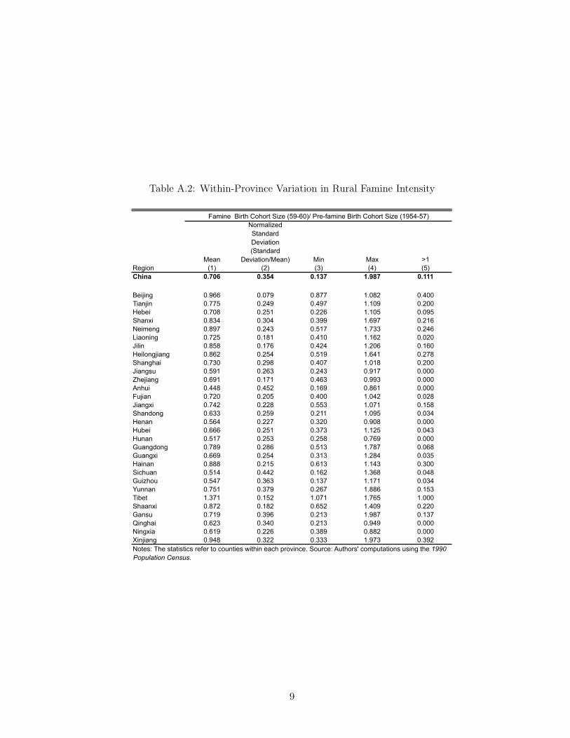
Table A.2: Within-Province Variation in Rural Famine Intensity

Mean

Normalized Standard Deviation (Standard

Deviation/Mean) Min Max >1Region (1) (2) (3) (4) (5)China 0.706 0.354 0.137 1.987 0.111

Beijing 0.966 0.079 0.877 1.082 0.400Tianjin 0.775 0.249 0.497 1.109 0.200Hebei 0.708 0.251 0.226 1.105 0.095Shanxi 0.834 0.304 0.399 1.697 0.216Neimeng 0.897 0.243 0.517 1.733 0.246Liaoning 0.725 0.181 0.410 1.162 0.020Jilin 0.858 0.176 0.424 1.206 0.160Heilongjiang 0.862 0.254 0.519 1.641 0.278Shanghai 0.730 0.298 0.407 1.018 0.200Jiangsu 0.591 0.263 0.243 0.917 0.000Zhejiang 0.691 0.171 0.463 0.993 0.000Anhui 0.448 0.452 0.169 0.861 0.000Fujian 0.720 0.205 0.400 1.042 0.028Jiangxi 0.742 0.228 0.553 1.071 0.158Shandong 0.633 0.259 0.211 1.095 0.034Henan 0.564 0.227 0.320 0.908 0.000Hubei 0.666 0.251 0.373 1.125 0.043Hunan 0.517 0.253 0.258 0.769 0.000Guangdong 0.789 0.286 0.513 1.787 0.068Guangxi 0.669 0.254 0.313 1.284 0.035Hainan 0.888 0.215 0.613 1.143 0.300Sichuan 0.514 0.442 0.162 1.368 0.048Guizhou 0.547 0.363 0.137 1.171 0.034Yunnan 0.751 0.379 0.267 1.886 0.153Tibet 1.371 0.152 1.071 1.765 1.000Shaanxi 0.872 0.182 0.652 1.409 0.220Gansu 0.719 0.396 0.213 1.987 0.137Qinghai 0.623 0.340 0.213 0.949 0.000Ningxia 0.619 0.226 0.389 0.882 0.000Xinjiang 0.948 0.322 0.333 1.973 0.392

Famine Birth Cohort Size (59-60)/ Pre-famine Birth Cohort Size (1954-57)

Table 2: Cross-sectional Variation in Famine Severity Across Counties

Notes: The statistics refer to counties within each province. Source: Authors' computations using the 1990 Population Census.

9

Table A.3: The Correlation between Reported Grain Productivity and Mortality Rates AcrossProvinces – Robustness to Controls

(1) (2) (3) (4) (5)Ln Grain Production x Famine Dummy 0.187 0.200 0.251 0.172 0.185

(0.0517) (0.0667) (0.0929) (0.0569) (0.0708)[0.496] [0.531] [0.667] [0.456] [0.490]

Ln Grain Production -0.0273 -0.0354 -0.0504 -0.0224 -0.0309(0.0275) (0.0299) (0.0266) (0.0273) (0.0294)[-0.0312] [-0.0405] [-0.0576] [-0.0257] [-0.0354]

GLF Principal Component x Famine Dummy 0.0103 0.00992(0.0196) (0.0192)[0.0103] [0.00989]

GLF Principal Component -0.00221 -0.00226(0.00263) (0.00263)[-0.0115] [-0.0117]

Per Capita Sown Area Growth (x -1) x Famine Dummy 0.115(0.169)[0.0145]

Per Capita Steel Production Growth x Famine Dummy 0.0322(0.0815)[0.0164]

% Participate in Communal Dining x Famine Dummy -0.000355(0.00205)[-0.0108]

% Purged during 1957 Anti-Right Movement x Famine Dummy** 0.0192(0.0197)[0.0663]

Late Liberation Dummy x Famine Dummy 0.115(0.0711)[0.0386]

Ln Urban Population x Famine Dummy 0.150 0.150(0.130) (0.129)[0.394] [0.393]

Observations 483 483 483 483 483R-squared 0.946 0.946 0.949 0.947 0.947Joint: Ln Grain Production x 1959 Dummy + Ln Grain Production 0.160 0.165 0.201 0.149 0.154p-value 0.003 0.018 0.036 0.011 0.036

Dependent Variable: Ln Deaths in year t+1

Notes: The famine dummy is equal to one for the years 1958-1960. All regressions control for log total population, log urban population and year fixed effects. In columns (2) and (5), we control for the principal component of GLF indicators: the late liberation dummy, the % of the population that was purged during the 1959 Anti-Right movement, communal kitchen participation rates during 1958-59, the growth in steel production and the negative growth in area sown for agriculture during 1958-61. Robust standard errors are reported in parentheses. In column (3), we also control for all of the uninteracted effects of the GLF intensity proxies. **In column (3), the coefficients for anti-right and anti-right x famine dummy are multiplied by 1,000 for presentation purposes. Standardized coefficients are reported in italics and brackets. The sample includes an unbalanced panel of 13-17 provinces for the years 1953-82. The number of provinces vary across years due to missing values for the GLF variables, and because there is no mortality data for Beijing for 1953. Sources: See text.

10

Table A.4: Year-by-Year Correlations between Ln Constructed Grain Productivity and MortalityRates, and Ln Constructed Grain Productivity and Procurement Rates

(1) (2) (3) (4)coef se coef se

Ln Constructed Grain x Year Dummy

1954 0.103 (0.0592) 0.425 (0.0800)1955 -0.00420 (0.0212) 0.202 (0.0286)1956 0.0125 (0.0216) 0.161 (0.0291)1957 -0.0514 (0.0389) 0.403 (0.0526)1958 -0.0292 (0.0384) 0.317 (0.0519)1959 0.0628 (0.0474) 0.548 (0.0640)1960 0.277 (0.0489) 0.686 (0.0659)1961 -0.0230 (0.0506) 0.725 (0.0684)1962 -0.0457 (0.0505) 0.629 (0.0683)1963 -0.0310 (0.0512) 0.560 (0.0692)1964 0.0292 (0.0533) 0.492 (0.0720)1965 0.0170 (0.0512) 0.423 (0.0693)1966 -0.0303 (0.0503) 0.328 (0.0681)1967 0.0153 (0.0499) 0.394 (0.0675)1968 -0.0589 (0.0492) 0.352 (0.0666)1969 -0.0999 (0.0510) 0.362 (0.0690)1970 -0.0535 (0.0505) 0.382 (0.0682)1971 -0.0562 (0.0501) 0.303 (0.0678)1972 -0.0709 (0.0496) 0.293 (0.0670)1973 -0.0562 (0.0482) 0.376 (0.0652)1974 -0.0566 (0.0485) 0.314 (0.0655)1975 -0.0696 (0.0437) 0.231 (0.0591)1976 -0.130 (0.0481) 0.259 (0.0649)1977 -0.0798 (0.0468) 0.291 (0.0633)1978 -0.112 (0.0485) 0.423 (0.0656)1979 -0.0996 (0.0473) 0.317 (0.0639)1980 -0.0913 (0.0460) 0.312 (0.0620)1981 -0.0904 (0.0459) 0.335 (0.0620)1982 -0.0867 (0.0468) 0.420 (0.0632)

-0.0567 (0.0463) 0.399 (0.0625)ObservationsR-squared

Dependent Variables

Notes: All regressions control for log total population, log urban population and year fixed effects. Robust standard errors are presented in the parentheses.These estimates use a balanced province-level panel that includes 19 provinces and the years 1953-1982, with the exception that there is no mortality data for Beijing in 1953. Sources: CDSM50 (1999), the Ministry of Agriculture (1983) and the authors' computations.

5690.960

Ln Death in Year t+1 Procurement Rate

5690.722

11

Tab

leA.5:Year-by

-YearCorrelation

sbe

tweenSu

rvivor

Birth

Coh

ortSizesan

dNatural

Con

dition

s

(1)

(2)

(3)

(4)

(5)

(6)

Coe

ffici

ent

Std

. Err.

Coe

ffici

ent

Std

. Err.

Coe

ffici

ent

Std

. Err.

Sui

tabi

lity

xLn

Spr

ing

Tem

pera

ture

xLn

Spr

ing

Rai

nfal

l x19

500.

333

(0.0

528)

1950

-0.9

85(0

.259

)19

500.

0581

(0.0

475)

1951

0.29

2(0

.050

3)19

51-0

.345

(0.2

58)

1951

0.08

28(0

.049

4)19

520.

278

(0.0

442)

1952

-0.3

82(0

.215

)19

520.

0449

(0.0

346)

1953

0.14

3(0

.040

9)19

530.

122

(0.2

05)

1953

0.02

68(0

.037

7)19

540.

0389

(0.0

443)

1954

0.27

7(0

.267

)19

54-0

.088

7(0

.043

3)19

550.

134

(0.0

440)

1955

-0.4

21(0

.173

)19

550.

0206

(0.0

414)

1956

-0.0

517

(0.0

414)

1956

-0.0

372

(0.1

63)

1956

0.10

9(0

.037

2)19

57-0

.290

(0.0

704)

1957

-0.3

04(0

.210

)19

570.

0828

(0.0

521)

1958

-0.4

52(0

.087

7)19

58-1

.412

(0.2

60)

1958

0.11

1(0

.068

3)19

59-0

.416

(0.1

14)

1959

-1.7

12(0

.350

)19

59-0

.148

(0.0

906)

1960

-0.2

11(0

.088

2)19

60-0

.470

(0.4

66)

1960

-0.0

0755

(0.0

817)

1961

-0.0

471

(0.0

498)

1961

0.12

4(0

.225

)19

610.

131

(0.0

440)

1962

0.08

25(0

.043

0)19

620.

360

(0.1

93)

1962

0.08

70(0

.029

9)19

63-0

.073

1(0

.042

6)19

630.

815

(0.2

04)

1963

0.03

56(0

.046

1)19

64-0

.063

3(0

.044

7)19

640.

827

(0.2

16)

1964

0.02

80(0

.058

4)19

65-0

.025

2(0

.052

6)19

651.

121

(0.1

99)

1965

0.01

37(0

.047

6)

Obs

erva

tions

R-s

quar

ed

Dep

ende

nt V

aria

bles

: Ln

Birt

h C

ohor

t Siz

e in

yea

r t+1

8176

0.91

8

The

regr

essi

on c

ontro

ls fo

r log

ave

rage

cou

nty

birth

coh

ort s

ize,

yea

r and

pro

vinc

e fix

ed e

ffect

s. T

he s

tand

ard

erro

rs a

re c

lust

ered

at t

he c

ount

y le

vel.

Not

es: T

he e

stim

ates

use

a c

ount

y-le

vel p

anel

of b

irth

coho

rts th

at in

clud

es 5

11 c

ount

ies

for t

he y

ears

195

0-66

con

stru

cted

from

the

1990

Pop

ulat

ion

Cen

sus,

the

Terr

estri

al A

ir Te

mpe

ratu

re a

nd P

reci

pita

tion:

Mon

thly

and

Ann

ual T

ime

Ser

ies

and

the

FAO

GA

EZ

data

base

.

12

Figure A.1: Constructed Production vs. Reported Production for the four GLF Years 1958-1961

05

00

10

00

15

00

Co

nstr

ucte

d G

rain

Pro

du

ctio

n (

Me

tric

To

ns)

0 500 1000 1500Reported Grain Production (Metric Tons)

(a) 1958

05

00

10

00

15

00

Co

nstr

ucte

d G

rain

Pro

du

ctio

n (

Me

tric

To

ns)

0 500 1000 1500Reported Grain Production (Metric Tons)

(b) 1959

05

00

10

00

15

00

Co

nstr

ucte

d G

rain

Pro

du

ctio

n (

Me

tric

To

ns)

0 500 1000 1500Reported Grain Production (Metric Tons)

(c) 1960

05

00

10

00

15

00

Co

nstr

ucte

d G

rain

Pro

du

ctio

n (

Me

tric

To

ns)

0 500 1000 1500Reported Grain Production (Metric Tons)

(d) 1961

13

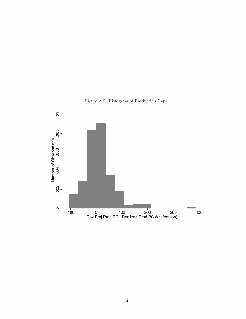
Figure A.2: Histogram of Production Gaps

0.0

02

.004

.006

.008

.01

Num

ber

of O

bserv

ations

-100 0 100 200 300 400Gov Proj Prod PC - Realized Prod PC (kgs/person)

14