The Institute of Cost Accountants of India - icmai-rnj.in
236
The Institute of Cost Accountants of India (Statutory body under an Act of Parliament) Volume 40, December 2014 ISSN 2230 9241 www.icmai.in RESEARCH BULLETIN
-
Upload
khangminh22 -
Category
Documents
-
view
1 -
download
0
Transcript of The Institute of Cost Accountants of India - icmai-rnj.in
The Institute of Cost Accountants of India(Statutory body under an Act of Parliament)
Volume 40, December 2014
I S S N 2 2 3 0 9 2 4 1
www.icmai.in
RESEARCHBULLETIN

The Institute of Cost Accountants of India(Statutory body under an Act of Parliament)
Volume 40, December 2014
I S S N 2 2 3 0 9 2 4 1
www.icmai.in
RESEARCHBULLETIN


Disclaimer The Institute assumes no responsibility for any act of copying or reproduction, whether fully or partially, of any write up / research paper which is not the original work of the author. The write up / research papers published in good faith on the basis of declaration furnished by the authors.
All rights reserved. No part of this publication may be used or reproduced in any manner whatsoever without permission in writing from The Institute of Cost Accountants of India.
Price of Single Copy: ` 400.00 onlyAnnual Subscription (for four volumes): ` 1200.00 p.a.Courier Charges: ` 200.00 p.a. for four volumes Month of Publication: December, 2014© 2014 The Institute of Cost Accountants of India

I am in high spirits to bring forth the present volume of the Research Bulletin of the Institute. The publication contains well researched and thought provoking articles on a variety of relevant issues for researchers, academicians and professionals.
Sustainable Cost Management (SCM) provides stakeholders with the ability to manage and align costs with their business strategies on a continuous basis. This can yield substantial benefits, establishing a framework for continuous improvement and ongoing performance measurement improving core and support processes while achieving enhanced customer satisfaction levels by reducing costs.
The CMAs with expertise knowledge play an indispensable role in value maximization and sustainable cost management process. They can typically serve as member of team leadership and is considered a technical professional within the organization. CMAs play a crucial role in the monitoring and control of cost and efficiency of the routine processes and as well as on-off jobs and projects undertaken by an organization and lays great emphasis on accountability through effective performance measurement.
In this edition, a wide array of topics based on Capital Budgeting, Corporate Ethics, Performance Management, Stock Market, Mutual Fund, Foreign Direct Investment, Inflation, Education and Agriculture have been inserted.
Hope this volume encourages readers to board on a lifelong journey of learning and enriching their knowledge base.
CMA (Dr.) A.S. Durga PrasadPresident
The Institute of Cost Accountants of India.
Foreword


It gives me an immense pleasure to place before you the 40th volume of Research Bulletin of the Institute. Our Research Bulletin mainly accentuate on pragmatic research papers and case studies on cost, management and financial issues.
Research means creativity accomplished on a systematic basis in order to increase the stock of knowledge, including knowledge of man, culture and society, and the use of this stock of knowledge to devise new applications. Our aim is to draw attention to the vitality in environmental, social, economical and market-related issues through our Research Bulletin, so that the society can analyze the surroundings, adapt the change in a better manner and can take decisions strategically.
I would like to express my appreciation to my fellow members of the Research, Innovation and Journal Committee, esteemed members of the Review Board, the eminent contributors and the entire research team of the Institute for their earnest effort and support to publish this volume in time.
I am sure the readers will find the Bulletin useful and would love to go through all the articles and I welcome the readers to put forward their valuable feedback to enrich Research Bulletin further.
CMA Manas Kumar ThakurChairman, Research, Innovation & Journal Committee
The Institute of Cost Accountants of India
Chairman’s Communiqué

Greetings!!!
We are glad to bring out the current volume of the Research Bulletin, Vol. 40, December, 2014 issue, an offering of the Directorate of Research & Journal of the Institute. We publish both theme based and non theme based articles on the blazing issues. Inputs are mainly received both from academicians and the corporate stalwarts. Our aim is to highlight the dynamism in environment, social, economy and market-related issues, so that the society can analyze the surroundings, adapt the change in a better manner and can take decisions strategically.
We are extremely happy to convey that from 2015 onwards ‘Research Bulletin’ will become quarterly publication in order to match with the international standards. As such we would be publishing the next issue in April 2015, on the theme “Capital Market” which would be a collaborative publication in association with National Institute of Securities Markets (NISM), an educational institute of SEBI.
We look forward to constructive feedback from our readers on the articles and overall development of the Research Bulletin. Please send your mails at [email protected]. We thank all the contributors of this important issue and hope our readers enjoy the articles.
CMA (Dr.) Debaprosanna NandyDirector (Research & Journal)
The Institute of Cost Accountants of India
Editors's Note


CMA Dr. AS Durga Prasad President & Permanent Invitee
CMA PV BhattadVice President & Permanent Invitee
CMA Manas Kumar Thakur Chairman
CMA Rakesh SinghMember
CMA Sanjay GuptaMember
CMA Dr. PVS Jagan Mohan RaoMember
CMA DLS SreshtiMember
CMA Dr. Sanjiban BandhyopadhyayaMember
Shri Suresh Pal Govt. Nominee
Secretary to the CommitteeCMA Dr. Debaprosanna NandyDirector (Research & Journal)
Research, Innovation & Journal Committee: 2014-15


Prof. Amit Kr. MallickEx- Vice Chancellor, Burdwan University
Dr. Asish K. BhattacharyyaAdvisor, Advanced Studies, The Institute of Cost Accountants of India
Dr. Ashoke Ranjan ThakurVice Chancellor, Techno India University, West Bengal
Dr. Bappaditya MukherjeeManaging Editor, Journal of Emerging Market Finance, Delhi
Dr. Dilip Kr. DattaDirector, Sayantan Consultants Pvt. Ltd., Kolkata
Dr. Malavika DeoProfessor, Department of Commerce, Pondicherry Central University, Puducherry
Dr. Nagaraju GotlaAssociate Professor, National Institute of Bank Management, Pune
Dr. P.K.JainProfessor, Department of Management Studies, IIT Delhi
Dr. Sankarshan BasuAssociate Professor, IIM-Bangalore
Dr. Sreehari ChavaDirector, Santiniketan Business School, Nagpur
Shri V.S.DateyExpert on Corporate Laws & Taxation, Nashik
Editor : CMA Dr. Debaprosanna NandyDirector (Research & Journal)
Joint Editor : CMA Dr. Sumita ChakrabortyJt. Director (Research)
Editorial Board


CMA Arindam BanerjeeFellow Member, Institute of Cost Accountants of [email protected]
CMA Ashish P Thatte Practicing Cost Accountant, Mumbai, [email protected] Dr. Ashok Joshi Director, INDSEARCH Pune, Maharashtra.
Dr. Badar Alam IqbalProfessor, Dept. of Commerce, Aligarh Muslim University, Uttar [email protected]
Ms. Baishakhi BardhanResearch Scholar, Department of Business Management, University of Calcutta, West [email protected]
Shri Dhruba Charan HotaAssistant Professor, Iswar Chandra Vidyasagar College, Belonia, Tripura
Dr. Dipen RoyAssociate Professor, Department of Commerce, University of North Bengal, West [email protected]
Mr. H.M. Kamrul HassanLecturer, Department of Marketing Studies and International Marketing, University of Chittagong, [email protected]
Shri Lalit GuptaStudent, MBA Programme, Department of Management Studies, IIT Delhi, New [email protected]
Our Contributors in this Issue

Dr. Laxmi Narayan KoliAssociate Professor, Deptt. of Accountancy & Law, Faculty of Commerce, Dayalbagh Educational Institute [Deemed University], Uttar [email protected]
Dr. Luciana Aparecida BastosAssociate Professor, Department of Economics,UNESPAR, Brazil [email protected]
Dr. M. BabuAssistant Professor, Department of Commerce and Financial Studies, Bharathidasan University, Tamil [email protected]
Dr. Madhumita Sen GuptaDeputy Director (President Office), The Institute of Cost Accountants of India (ICAI), [email protected]
Dr. Malabika DeoProfessor, Department of Commerce, Pondicherry University, [email protected]
Mr. Martin BernardPhD Scholar, Department of Commerce, Pondicherry University, Puducherry [email protected]
Mr. Nayyar RahmanUGC Junior Research Fellow, Department of Commerce, A.M.U., Uttar Pradesh
Dr. P.K. JainProfessor, Department of Management Studies, IIT Delhi, New [email protected]
Our Contributors in this Issue

Ms. Pooja ChoudharyResearch Scholar, Faculty of Commerce, Banaras Hindu University, Uttar [email protected]
CMA (Dr.) Samyabrata Das Assistant Professor, Department of Commerce, New Alipore College, West [email protected]
Prof. S. M. Salamat Ullah BhuiyanProfessor, Department of Marketing Studies and International Marketing, University of Chittagong, [email protected]
Shri S. SrinivasanPh.D Scholar in Management, Department of Commerce and Financial Studies, Bharathidasan University, Tamil [email protected]
Dr. Sudipta GhoshAssistant Professor, Department of Commerce (UG & PG), Prabhat Kumar College, West [email protected]
Shri Zapan BaruaLecturer, Department of Marketing Studies and International Marketing, University of Chittagong, [email protected]
Our Contributors in this Issue

Capital Budgeting Practices of Corporate Enterprises in India: An Empirical StudyDipen Roy, Dhruba Charan Hota
Corporate Ethical Reporting Practices and Pattern in IndiaLaxmi Narayan Koli
Equity Share Price Efficiency of Indian Banking SectorM. Babu, S.Srinivasan
Financial Performance of Software Industry in India : A Study in the Context of ProfitabilityLalit Gupta, P.K. Jain
Foreign Direct Investment in Indian Scenario : An Empirical Study of Service SectorArindam Banerjee
Higher Education in Private Universities of Bangladesh: Emergence, Reality and Policy Guidelines S. M. Salamat Ullah Bhuiyan, H.M. Kamrul Hassan, Zapan Barua
Impact of Liberalization Process on Growth, Instability, Extent of Diversification and Total Factor Productivity Growth of the Agricultural SectorMadhumita Sen Gupta
India’s Standing in Global Life Insurance Market : A Brief AnalysisPooja Choudhary
Contents
21
35
61
51
83
97
109
133

Inflation Trends in BRICS NationsBadar Alam Iqbal, Luciana Aparecida Bastos, Nayyar Rahman
Long Term Price Momentum, Early, and Late Strategies in Indian Market Stock ReturnsMartin Bernard, Malabika Deo
Performance of Indian Mutual Funds: An Empirical Study of Select Equity Linked Saving SchemesSamyabrata Das
Performance of Manufacturing Industries in West Bengal During 1981 - 1998: An Empirical StudyBaisakhi Bardhan
Returns on Shareholders Equity of Select Industries in Liberal Economic Scenario: Empirical Evidence from IndiaSudipta Ghosh
Study of Balanced Scorecard as Performance Management System for Profit Maximization in Automobile, IT and Engineering IndustryAshok Joshi, Ashish P Thatte
Contents
145
163
175
187
195
211


1. Introduction
Future growth prospect and survival of a corpo-rate house depend, to a large extent, upon the success of its capital budgeting decision-making, where the decision-makers’ greatest emphasis is on economic evaluation of a long-term invest-ment proposal. Acceptance of many important projects such as investments in new business opportunities, renovation, replacement, tech-nology up-gradation, etc. depends upon the economic clearance after rigorous financial and technical appraisal.
To keep pace with growth and fight competition in the current framework of competitive market environment, capital budgeting is critically im-portant to every corporate house. If a corporate house makes correct capital budgeting decision in conformity with its strategic outlook, stability and growth eventually make the firm powerful and enable it to compete with rival firms. A good decision can lay the foundation for future success and pave the way towards increasing production, sales and profitability, while a wrong decision can create an unnoticed hole in its purse and lead to an eventual collapse and liquidation. Thus, taking a correct capital budg-eting decision is regarded to be an important pillar for fighting competition and running the business effectively.
Capital Budgeting Practices of Corporate Enterprises in India : An Empirical Study
Dipen RoyDhruba Charan Hota
Abstract
Capital budgeting is critically important to every corporate house operating in the era of competitive market environment. This article reports the result of a survey of capital budgeting of thirty companies listed on NSE. The results show that today nearly 83 percent of corporate houses use sophisticated DCF methods for economic evaluation of their investment proposals. It also shows that corporate houses today instead of relying on the theoretical superiority of a single, they use multiple methods and combine science with practical business prudence to be sure that the related investment proposal is safe to the company. Financing and capital budgeting decisions, being interlinked and inter-dependent, have been simultaneously studied in this paper to trace the presence of any link between sources of finance and choice of appraisal methods. The study also reveals that the corporate houses today give considerable emphasis on corporate strategy as a decision variable in choosing a long-term investment proposal.
Keywords
Capital Budgeting, Discounted Cash Flow Analysis, Strategic Investments, Financing Decision, Liquidity.
ESEARCH BULLETIN
21 Volume : 40 I December 2014

Since substantial irreversible expenditures are associated with the capital budgeting decisions, rigorous methods and analytical tools are to be used for arriving at the correct decision. How-ever, to face with the changes taking place in product and financial markets, old methods are getting continuously reviewed and updated. Given the forces operating in the market place, the relevant question is ‘do the companies follow scientific rules and methods of capital budgeting in India?’ This paper has been taken up to find answer to this question.
2. Quantitative Methods of Investment Appraisal
There are a number of methods for quantitative appraisal of investment proposals. Depending on the methodologies involved with them, the methods have been broadly classified into two categories, viz., DCF (Discounted Cash Flow) methods and Non-DCF methods. Methods like Internal Rate of Return (IRR), Modified Internal Rate of Return (MIRR), Net Present Value (NPV) and Net Terminal Value (NTV) belong to DCF category. On the other hand, Payback Period and Accounting Rate of Return (ARR) fall under Non-DCF category. The use of more advanced versions like MIRR and NTV is almost negligible (Patel B. M., 2000). Very recent research find-ings [i.e., Graham and Harvey (2002); George Kester and Geraldine Robbins (2011)] show that Financial Executives in the practical field use four methods such as IRR, NPV, Payback Period and ARR.
Focus of Payback Period is early recovery of invested sum, which results in strengthening the liquidity position of the firm. IRR represents the highest return an investment can generate and NPV gives the quantum of absolute value addi-tion. It shows each of the methods is designed to measure a specific feature of an investment, not all features together.
3. Literature Review
In India the credit of first published study in the area of capital budgeting decision-making in corporate sector goes to Porwal L S (1976). In early seventies of last century he noticed prevalence of traditional appraisal methods in quantitative evaluation of investment propos-als. He observed the largest number of firms to rely on Payback Period method, which is not theoretically recognised to be a sound method for project evaluation. From a study of a small sample of fourteen large Indian firms, Pandey I M (1989) arrived at almost similar results. His findings confirmed that the majority of the companies were still using Payback Period as the primary method for evaluation of projects. In addition to this, he also reported that about two-thirds of the companies using Payback Period method were simultaneously using Internal Rate of Return (IRR) as the secondary method. From a study of 64 firms of different sizes Shivaswamy M (1996) obtained almost same results once again.
However, very recent studies report a better trend consistent with modern theories of quantitative appraisal. In India the use of IRR has increased steadily. Anand Manoj (2002) found 85 % of the firms using IRR. In addition to using IRR, 67% of these companies were found to use Payback Period as a supporting second method. To the practicing managers popularity of Payback Peri-od is still very high. Presently instead of relying on a single method, firms have developed the trend of using multiple methods to be assured about the merit of an investment proposal (Patel B M, 2000). It is interesting to observe that the sum of percentages, as shown in the column marked for Porwal’s (1976) findings, is equal to 100%. But no ‘column total’ is 100% in respect of other studies. Due to simultaneous use of multiple methods, the sum of the percentage of popularity of various methods appears more than 100% in the studies of Prabhakar (1995) and Manoj Anand (2002).Chadwell-Hatfield et al (1997) from a study re-
ESEARCH BULLETIN
Volume : 40 I December 2014 22

Table 1: Trend in the use of Capital Budgeting Evaluation Techniques in India
Methods of Evaluation
Porwal L S (1976)
Shivaswami(1995)
Manoj Anand(2002)
Shah Kamini(2008)
ARR Payback NPV IRR Other
38%23%4%
27%8%
33%69%31%54%14%
34.0%67.5%66.3%85.0%35.0%
--66.7%55.6%74.1%7.4%
ported that 67% firms insisted that acceptable projects should have a shorter Payback Period in addition to passing NPV or IRR criterion. Table 1 reflects that for evaluation of capital projects, today the firms don’t rely on using a single eval-uation method. Patel B M (2000) observes that some of the Indian firms even use four to five methods before arriving at the final decision regarding acceptance or rejection of an invest-ment proposal. The findings reflect that today the firms tend to be more careful in choosing an investment proposal.
Table 1 given above reveals that since 1976 use of IRR has steadily increased in India. Its use is still increasing every day. Payback Period is the next most favoured technique. However, NPV is not so popularly used as IRR and Payback Period are used.
Gupta Sanjeev et al. (2007) conducts a study on 32 companies in Punjab. He observes that major-ity of the sample companies use non-discounted cash flow techniques like PBP and ARR. Only a few companies have been found to use DCF; of them very negligible number of companies were found to use NPV. The most preferred discount rate is WACC.Shah Kamini (2008) observes that almost all the companies are using now multiple techniques for evaluating their capital budgeting proposals. The researcher also observes that the companies prefer ‘IRR and NPV’ to Payback period method.
Interestingly she observes two different trends in choosing evaluation tools. She notes that for investing in new projects firms use IRR, PBP and NPV, while for expansion, replacement and modernization firms largely rely on Payback period method. She also notes that Sensitivity Analysis is the most important technique for risk analysis and scenario analysis as the second most important technique for this purpose.
Using a sample size of 75 companies, Gupta Divya (2013) shows that there is a positive relationship between frequency of usage of capital budgeting techniques and application of discounted cash flow techniques with the firm project size and social cost benefit analysis.
Yadav Vinod Kumar (2013) finds that in small-scale industries firms mainly use traditional payback period and Accounting Rate of Return instead of scientific evaluation methods like IRR and NPV.
3A : Trends in Developed Countries
Pike and Neale (1996) from the study of top 100 UK companies observed 54% companies to use IRR, whereas use of NPV was reported as low as 33% of firms surveyed. A chronological survey of studies made in USA reveals a clear trend of gradual increase in the use of sophisticated methods. Suk, Trevor and Seung (1986) found 49% and 21% of the companies to use IRR and
ESEARCH BULLETIN
Volume : 40 I December 201423

NPV respectively as primary methods for project appraisal. So, combined use of sophisticated DCF methods increased to 70%, which was just 7% in 1949. Some years later Bierman (1993) found 73 out of responding 74 sampled ‘Fortune 100’ companies to rely on use of Discounted Cash Flow methods. Especially IRR was found preferred to NPV. However, Payback period still remained as a very popular secondary method.
Studying a sample of 300 UK companies Arnold Glen C. and Hatzopoulos Panos D. (2000) ob-serves that the large UK corporations depend on modern methods of investment evaluation. They also notice prevalence of traditional, rule-of-thumb techniques, alongside DCF techniques.
Kaplan and Atkinson (2000) shows the mistakes committed in appraisal of new technology in-vestments. They observe that as new technology is risky, the managers, at the time of appraisal, either set a very low payback period or discount the future cash inflows at an abnormally high rate of discounting, which renders future inflows redundant and less useful for evaluation purpose.
Graham and Harvey (2002) observe that the highest percentage of corporate houses in the USA to depend on the use of IRR as primary method for evaluation of long-term investment projects.
Ryan Patricia A and Ryan Glenn P. (2002) exam-ine the methods of investment appraisal used by the Fortune 1000 companies. They find NPV as the most preferred (96%) method of appraisal followed by IRR. Side by side they find 74.5% of the companies to use Payback Period method. They observe that for handling risk the companies depend more on sensitivity analysis. Scenario analysis is found as the second best method in this process.
Brigham and Houston (2004) highlight the role of options in Capital Budgeting. According to
them, along with the results of quantitative eval-uation the options values are to be considered before making final ranking of mutually exclusive investments. They discuss various options like managerial option, re-investment option, flexibil-ity option, etc.
From a survey of companies listed on Irish Stock Exchange George Kester and Geraldine Robbins (2011) found almost 100 percent companies to use economically justified DCF methods, such as NPV and IRR, alone or in combination with non-DCF methods such as Payback Period.
On the basis of study on Swedish companies Hartwig (2012) observes that over time the use of sophisticated methods seems to be increasing and the use of unsophisticated methods de-creasing. This indicates that the theory-practice gap is gradually getting reduced. Hartwig’ main-ly studies compliance of accounting standards like IFRS in capital budgeting. He raises the issue that if evaluation is made on the basis of man-agers’ personal forecasts, it cannot be counted as reliable accounting information for reporting purpose.
Though in Western countries lots of studies have been made, but in India only limited number of studies have been done. To fill this gap the study has been undertaken.
4. Objective of the Study
The objective of the paper is to study capital budgeting practice of Indian corporate houses. Do the corporate houses use a single method or a combination of multiple methods? Obtaining a picture of present trend is the foremost objective of the study. The another important objective of the paper is to study financing and investment decisions simultaneously and trace if financing decision has any influence on capital budgeting decision. In addition to the above, the study has other two important objectives. These are: i)
ESEARCH BULLETIN
24Volume : 40 I December 2014
to find if the size of investment has some role in selection of evaluation method and ii) to assess the impact of corporate strategy on capital budgeting decisions.
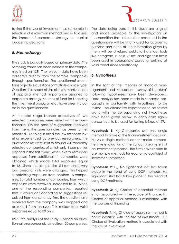
5. Methodology
The study is basically based on primary data. The sampling frame has been defined as the compa-nies listed on NSE. The relevant data have been collected directly from the sample companies through questionnaires. The questionnaire con-tains objective questions of multiple-choice type. Questions in respect of size of investment, choice of appraisal method, importance assigned to corporate strategy, sources of fund for financing the investment proposal, etc., have been includ-ed in the questionnaire.
At the pilot stage finance executives of two selected companies were visited with the ques-tionnaire. On the basis of suggestions received from them, the questionnaire has been further modified. Keeping in mind the low response lev-el as experienced by previous researchers, the questionnaires were sent to around 230 randomly selected companies, of which only 4 companies respond in the first round. After several reminders responses from additional 11 companies were obtained which made total responses equal to 15. Since the sample size still remained very low, personal visits were arranged. This helped in obtaining responses from another 16 compa-nies. So total number of companies, from which responses were received, increased to 31. Since one of the responding companies, reported that it would act according to suggestions re-ceived from consultancy firm, the questionnaire received from the company was dropped and excluded from analysis. This makes total valid responses equal to 30 only.
Thus, the analysis of the study is based on ques-tionnaire responses obtained from 30 companies.
The data being used in this study are original and made available to the investigators on the condition that information presented in the questionnaire will be strictly used for academic purpose and none of the information given by them will be divulged publicly. Statistical tools like histogram, z –test, χ2 test and sign test have been used in appropriate cases for arriving at valid conclusions scientifically.
6. Hypothesis
In the light of the ‘theories of financial man-agement’ and ‘subsequent survey of literature’ following hypotheses have been developed. Data analysis has been made in separate par-agraphs in conformity with hypotheses to be tested. The alternative hypotheses to be tested along with the corresponding null hypotheses have been given below. In each case signifi-cance level to be used for testing is fixed at 5%.
Hypothesis 1: H0: Companies use only single method to arrive at the final investment decision. H1: As a single method cannot make compre-hensive evaluation of the various parameters of an investment proposal, the firms have reason to use multiple methods for economic appraisal of investment proposals.
Hypothesis 2: H0: No significant shift has taken place in the trend of using DCF methods. H1: Significant shift has taken place in the trend of using DCF methods.
Hypothesis 3: H0: Choice of appraisal method is not associated with the source of finance. H1: Choice of appraisal method is associated with the sources of financing
Hypothesis 4: H0: Choice of appraisal method is not associated with the size of investment. H1: Choice of Evaluation method is associated with the size of investment
ESEARCH BULLETIN
25 Volume : 40 I December 2014

7. Data Analysis and Presentation
Data collection has been made during last five years, from 2009 to 2013. The data regarding use of appraisal methods by 30 companies have been initially compiled in Table 1. It shows that out of 30 companies surveyed 9 companies use IRR and Payback Period simultaneously. Another eight companies, in addition to using IRR and Payback period simultaneously, use NPV method too as an additional method to be more secured in arriving at the correct decision. That is, these latter 8 companies use three methods, viz., NPV, IRR and Payback Period simultaneously. Number of companies using only DCF method alone is just three; two of them are using IRR and one is using NPV. Therefore, though the Table 1 reflects that in aggregate 28 companies use sophisticat-ed DCF methods; but it does not confirm that the corporate houses substituted DCF method for non-DCF traditional methods. Use of non-DCF methods is still prevalent. The corporate houses use DCF and non-DCF methods simultaneously to cover appraisal of the maximum number of parameters of an investment, as possible.
Table 2: Number of Companies and Appraisal Methods Used
Appraisal Methods Used
Number of firms
IRR, Payback Period 9 IRR, NPV, Payback 8RR, NPV 2IRR, NPV, Payback, ARR
3
IRR 3NPV, Payback period 2NPV 1Payback period 2ARR 0Total Number of Firms 30
Only two companies report that they use only non-DCF Payback Period method alone. Data reveals that the firms place greater reliance on combined use of DCF and non-DCF methods to avoid the risk of taking a wrong decision. 7.1: Simultaneous Use of Multiple Methods
Out of the 30 firms surveyed, only six firms have been found to use a single method for project appraisal. Remaining 24 companies use multiple methods for appraisal of their project proposals. Three companies have been found to use four methods simultaneously to arrive at their final decision. Thirteen companies have been found to use 2 methods, while eight companies have been found to use three methods. The data regarding use of multiple methods have been shown in Fig. 1 with the help of histogram.
Use of multiple methods can be explained as an attempt to taking into account the different attributes of an investment. From Table 1 it is observed that vast majority of the companies use Payback Period method in addition to DCF methods like IRR and NPV. It indicates that major-ity of the companies insist on liquidity in addition to profitability. Since 80% companies use multiple methods, the alternative hypothesis that Indian Companies use multiple methods for investment appraisal is accepted. Statistical validity of the inference has been established through a non-parametric sign test as given below. Firms using multiple methods are assigned plus sign and those using single method are assigned negative sign.
Number of Plus (+) sign, X = 24 Number of Minus (–) sign = 6 Sample size, n = 30H0: Probability of + sign is equal to 0.5, Symbolically, H0: P(+) = 0.50H1: Probability of + sign is greater than 0.5,
ESEARCH BULLETIN
26Volume : 40 I December 2014

Fig. 1: The Trend of Using Multiple Evaluation Methods
Symbolically, H1: P(+) > 0.50
For right-tailed test 5% Critical Value of Z = 1.645
Since computed Z is greater than critical value (1.645), the alternative hypothesis that the firms depend on the use of multiple methods for eval-uation of projects has been accepted.
7.2: Shifting Trends towards Scientific Methods
Data reveal that the highest percentage of companies uses IRR. The vast majority of the com-panies have been found to use IRR. The second equally important method is Payback Period. With different combinations of other methods, 24 companies have been found to use Payback Period. In percentage terms popularity of both IRR and Payback are 83% and 80% respectively. Compared to IRR, popularity of NPV to Indian companies is as low as 53% only.
Table 3: Percentage of Firms using Various Appraisal Method
Methods Number of Firms Using
Percentage of Users
IRR 25 83%Payback 24 80%NPV 16 53%ARR 3 10%DCF = NPV + IRR
28 93%
Only 16 companies indicate that they use NPV method. The data regarding popularity of various methods have been shown in Table 2. Popularity of the methods in per-centage terms have also been shown by a histogram as shown in Fig. 2.If we classify the data given in Table 1 in terms users of DCF and non-DCF methods, we find that only 2 companies do not use any DCF method. That is, out of 30 companies, 28 companies use DCF methods, alone or in combination with oth-er DCF and/or non-DCF methods. That is, overall 93% companies use sophisticated DCF methods. If this outcome is compared with the findings of Porwal (1976), which was just 31%, the difference
ESEARCH BULLETIN
27 Volume : 40 I December 2014

Fig. 2: Popularity of Various Appraisal MethodsD
egre
e of
Pop
ular
ity
appears highly significant. It can be confidently concluded that significant shift has taken place in respect of the use of DCF methods. Data gathered are quite enough to arrive at the con-clusion. Following statistical test has been made to make the inference statistically valid.
p1 = proportion of DCF users as per Porwal’s study = 0.31n1 = sample size in Porwal’s study = 45p2 = proportion of DCF users as per present study = 0.93n2 = sample size in the present study = 30
H0: P2 = P1
H1: P2 > P1
The test result supports alternative hypothesis. It can be safely concluded that since 1976 a significant shift has taken place in favour of using sophisticated DCF methods in capital bud-
geting. Compared to findings of Anand Manoj (2002), the difference is not significant. It leads to a conclusion that the major shift towards use of scientific methods has taken place in the 90s of the last century, when major liberalization pro-grammes were launched. However, the trend of using scientific methods what was set in 1990s is still being carried on in 21st century with some marginal improvements.
7.3: Relationship between Method of Financing and Choice of Appraisal Method
In the questionnaire an effort was made for ob-taining input regarding means of financing the investment proposals. Equity capital mobilised from new issue can be good source of financing new projects. However, following sub-prime crisis in 2008, as condition of capital market appeared unattractive, initial public offer in the primary market was almost negligible. The companies surveyed had no history of raising equity capital from primary market during the period of survey. The financing alternatives that were available to
28
ESEARCH BULLETIN
Volume : 40 I December 2014

them were confined to borrowing and retained earnings only. Data so obtained from the com-panies in respect of their mode of financing has been tabulated below:
Table 4: Modes of Financing
Modes of Financing Number of Companies
100% Loan Financing 2
Internal Fund Plus Loan Financing
23
100% Internal Fund 5
Table 4 shows that 25 firms (83%) finance the pro-ject proposals through loan financing. Of them 7% of the companies use 100% loan financing and remaining 76% companies combine internal fund with borrowing to finance the investments. These 25 firms taking loan, in part or fully, use multiple methods for economic evaluation of project proposals. 22 out of 25 borrowing firms report that they use IRR, alone or in combination with other methods, while only 12 firms report that they use NPV, alone or in combination with other methods.:
Table.5: Appraisal Method Used by Firms Financing Investment through
Borrowing
IRR NPV Total Number of Firms 22 12 25
Percentage (%) 88% 48%
It reflects that in the present industrial scenario, majority of the companies use loan capital for financing their investment proposals. While a firm is going to borrow, it is essential on the part of the companies to know at what highest rate they can make a fresh borrowing. In other words, to them it is essential to know if the project return
will be more than the rate of borrowing. To meet this requirement IRR acts as a good yardstick. It appears from the above table that there is a relationship between the selection of evaluation method and mode of financing the investment. Firms taking loan from market have reason to use IRR instead of NPV. This is statistically confirmed through Chi-square test at 5% level of signifi-cance.
Computed χ2 = 7.24 > Critical Value, 3.84 with 1 d. f.
In the backdrop of liberalization our findings appear relevant in the light of Leverage Ag-gressive Hypothesis (Brander and Lewis, 1986; Maksimovic, 1986), which states that as compet-itive situation and rivalry become dominant in market, firms use cheaper loan financing to fight product-market competition.
The statistical result informs that choice of ap-praisal method is not independent of method of financing. According to opinion of finance ex-ecutives, IRR gives more transparent idea about the outcome of a financial decision. IRR is the most popular method of investment evaluation because of its clarity. Ross, Westerfield and Jor-dan (2002) correctly highlight this with a simple instance. According to them, a finance execu-tive may simply report to the board of directors that new investment will fetch 20% return (given, IRR = 20%). This may somehow seem simpler than telling that at 10% discount rate the investment has the potential of producing NPV of certain amount, viz., $250 million.
Theoretically neither IRR is better than NPV, nor NPV’ is better than ‘IRR’. There is no rational reason behind identifying one of them as better, because both the measures are obtained from the same valuation equation. However, in the light of practical usefulness, IRR can be treated to be better than NPV. Very recent findings re-flect this truth. See Table 6 as given below:
29
ESEARCH BULLETIN
Volume : 40 I December 2014

Table 6: The Recent Trend Showing Popularity of IRR
Serial No. Author Year Most preferred
Method
1 Porwal L S (1976) 1976 ARR
2 Wong, Farragher and Leung (1987) 1987 PBP , ARR
3 Prabhakara Babu & Sharma A (1996) 1996 IRR
4 Colin Drury and Mike Tayles (1996) 1996 IRR
5 Kester, George W & Chong Tsui Kai (1996) 1996 IRR, PBP
6 Graham and Harvey (2001) 2001 IRR, NPV
7Cooper William D., Morgan Robert G.,Regman Alonzo, Smith Margart (2001)
2001 IRR
8 Ryan Patricia A and Ryan Glenn P. 2002 2002 NPV
9 Anand Manoj (2002) 2002 IRR10 Hogaboam, Liliya S. and Shook S R. (2004) 2004 IRR
11 Truong G., Partington and Peat M. 2006 2006 NPV, PBP
12 Shah Kamini (2008) 2008 IRR, NPV
Source: Shah Kamini (2008), edited partly to accommodate the recent findings only.
Note; PBP = Payback Period, IRR = Internal Rate of Return, NPV = Net Present Value
ESEARCH BULLETIN
7.4: Relationship between Selection of Appraisal Method and Size of Investment
In this paragraph the relationship between selection of Appraisal Method and Size of Invest-ment has been examined. In the questionnaire a question asking information regarding size of investment was listed. Companies were asked to give data on the sizes of their capital budgets in the last three years (2010 – 2013). Five compa-nies out of 30 companies surveyed abstain from giving input on this issue. On the basis of the re-sponses received from remaining 25 companies, size of average investment of each company was determined. Then on the basis of size of investments the companies have been grouped into two categories, one group having average investment below Rs 500 million and another
group having investment above Rs 500 million. Use of various methods by these two groups of companies has been enlisted in the table below:
Table 7: Size of Investment and Method of Appraisal
Appraisal Method
X< Rs 500 ml
X> Rs 500 ml Total
IRR 12 11 23NPV 5 10 15PBP 11 10 21Total 28 31 59
Note: Figures indicate number of companies using respective methods
To test existence of association between size of investment and choice of appraisal method
30Volume : 40 I December 2014
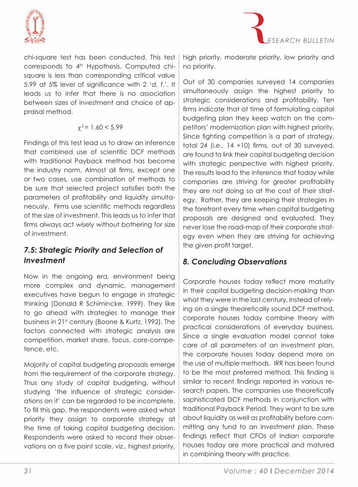
chi-square test has been conducted. This test corresponds to 4th Hypothesis. Computed chi-square is less than corresponding critical value 5.99 at 5% level of significance with 2 ‘d. f.’. It leads us to infer that there is no association between sizes of investment and choice of ap-praisal method.
χ2 = 1.60 < 5.99
Findings of this test lead us to draw an inference that combined use of scientific DCF methods with traditional Payback method has become the industry norm. Almost all firms, except one or two cases, use combination of methods to be sure that selected project satisfies both the parameters of profitability and liquidity simulta-neously. Firms use scientific methods regardless of the size of investment. This leads us to infer that firms always act wisely without bothering for size of investment.
7.5: Strategic Priority and Selection of Investment
Now in the ongoing era, environment being more complex and dynamic, management executives have begun to engage in strategic thinking (Donald R Schimincke, 1999). They like to go ahead with strategies to manage their business in 21st century (Boone & Kurtz, 1992). The factors connected with strategic analysis are competition, market share, focus, core-compe-tence, etc.
Majority of capital budgeting proposals emerge from the requirement of the corporate strategy. Thus any study of capital budgeting, without studying ‘the influence of strategic consider-ations on it’ can be regarded to be incomplete. To fill this gap, the respondents were asked what priority they assign to corporate strategy at the time of taking capital budgeting decision. Respondents were asked to record their obser-vations on a five point scale, viz., highest priority,
high priority, moderate priority, low priority and no priority.
Out of 30 companies surveyed 14 companies simultaneously assign the highest priority to strategic considerations and profitability. Ten firms indicate that at time of formulating capital budgeting plan they keep watch on the com-petitors’ modernization plan with highest priority. Since fighting competition is a part of strategy, total 24 (i.e., 14 +10) firms, out of 30 surveyed, are found to link their capital budgeting decision with strategic perspective with highest priority. The results lead to the inference that today while companies are striving for greater profitability they are not doing so at the cost of their strat-egy. Rather, they are keeping their strategies in the forefront every time when capital budgeting proposals are designed and evaluated. They never lose the road-map of their corporate strat-egy even when they are striving for achieving the given profit target.
8. Concluding Observations
Corporate houses today reflect more maturity in their capital budgeting decision-making than what they were in the last century. Instead of rely-ing on a single theoretically sound DCF method, corporate houses today combine theory with practical considerations of everyday business. Since a single evaluation model cannot take care of all parameters of an investment plan, the corporate houses today depend more on the use of multiple methods. IRR has been found to be the most preferred method. This finding is similar to recent findings reported in various re-search papers. The companies use theoretically sophisticated DCF methods in conjunction with traditional Payback Period. They want to be sure about liquidity as well as profitability before com-mitting any fund to an investment plan. These findings reflect that CFOs of Indian corporate houses today are more practical and matured in combining theory with practice.
ESEARCH BULLETIN
31 Volume : 40 I December 2014

Findings reveal that there exists a relationship between sources of finance and methods of ap-praisal. Firms depending on loan make greater use of IRR method than NPV. Our findings are in conformity with the propositions of Leverage Aggressive Hypothesis. However, no relationship exists between size of investment and choice of appraisal method. It leads us to conclude that the firms are equally serious even when fund involved with an investment plan is low. Finally, the study confirms that now in the ongoing era, at the time of choosing a long-term investment proposal the companies assign the highest priority to their corporate strategy even when they are under the compulsion to pursue a given profitability target.
References
Anand Manoj (2002): Corporate Finance Practices in India: A Survey, Vikalpa, Vol. 27, No. 4.
Arnold Glen C. and Hatzopoulos Panos D.(2000): The theory-practice gap in capital budgeting: evidence from the United Kingdom, Journal of Business Finance & Accounting, 27(5) & (6), June/July 2000, 0306-686X, pp. 603-626.
Bierman (1993): Capital Budgeting in 1992: A Survey, Financial Management, Vol. 22 No. 1 pp.13-28.
Boone & Kurtz (1992): Management, McGraw Hill Inc, New York. p. 25.
Brander, James A and Lewis, Tracy R (1986): Oligopoly and Financial Structure: the Limited Liability Effect” American Economic Re-view, vol.76, pp. 956-70.
Brigham Eugene F and Houston Joel F (2004): Fundamentals of Financial Management, Thomson, South-Western, USA, pp. 453-473.
Chandwell-Hatfield Patricia, Goitein Bernard, Horvath Philip, Webster Allen (1997): Fi-nancial Criteria, Capital Budgeting Techniques and Risk Analysis of Manufacturing Firms, Journal
of Applied Business Research, pp.95-104.
Colin Drury and Mike Tayles (1996) UK capital budgeting practices: some additional survey evidence, European journal of finance 2, pp 371-388.
Cooper William D., Morgan Robert G., et al (2001) Capital budgeting models: Theory Vs. Practice; Business Forum, 2001, Vol. 26, Nos. 1,2, pp. 15-19.
Donald R Schimincke (1999): Strategic Thinking: A Perspective for Success, Manage-ment Review, August, pp. 16-19.
George Kester and Geraldine Robbins (2011): Capital Budgeting Practices of Listed Irish Companies, Insights from CFOs on their in-vestment appraisal techniques. Accountancy Ireland, February, Vol. 43, No. 1 pp. 28-30.
Graham and Harvey (2002): How do CFOs make Capital Budgeting and Capital Structure Decisions? Journal of Applied Corpo-rate Finance, Vol. 15 No. 1, Spring.
Gupta Sanjeev, Batra Roopali and Shar-ma Manisha,”Capital Budgeting Practices in Punjab-based Companies, The ICFAI Journal of Applied Finance, February 2007, Vol. 13, No.2, pp. 57-70.
Gupta Divya ( 2013): Impact of Project size and social Cost Benefit Analysis on Capital Budgeting Decision of Indian Firms, Indian Jour-nal of Finance, Vol. 7, No. 10, pp. 45-53.
Hartwig, F. 2012. Four Papers on Top Man-agement’s Capital Budgeting and Accounting Choices in Practice Företagsekonomiska insti-tutionen. Doctoral thesis / Företagsekonomiska institutionen, Uppsala universitet 153 Uppsala.
Hogaboam, Liliya S. and Shook S R. (2004): Capital budgeting practices in the U.S. forest products industry: A reappraisal, Forest Products Journal, December 2004,Vol.54, No. 12, pp 149-158.
Kaplan Robert S and Atkinson Anthony A (2000): Justifying Investment in New Technology,
ESEARCH BULLETIN
32Volume : 40 I December 2014

in Advanced Management Accounting, Pren-tice Hall of India, New Delhi, pp. 473-492.
Kester, George W & Chong Tsui Kai (1996): Capital budgeting practices of listed firms in Singapore, Singapore Management Review, pp 9-23.
Maksimovic, Vojislav ( 1986): Optimal Capital Structure in Oligopolies, Ph.D. disserta-tion, Harvard University.
Pandey I M (1989): Capital Budgeting Practices of Indian Companies, MDI Manage-ment Journal, Vol.2, No. 1 pp. 36-48.
Patel B.M. (2000): Project Management, Vikash Publishing House, New Delhi.
Pike and Neale (1996): ‘A Longitudinal Survey of Capital Budgeting Practices’ in Cor-porate Finance and Investment: Decisions and Strategies, PHI, pp. 172-180.
Porwal L S (1976): Capital Budgeting in India, Sultan Chand, New Delhi, 1976.
Prabhakara Babu & Sharma A (1996): Capital budgeting Practices in Indian Industry, ASCI Journal of Management, Volume 25, 1996 downloaded from address http://www.journal.asci.org.in/vol.25(1996).v25_1_pra.htm.
Ross, Westerfield and Jordan (2002): Fun-damentals of Corporate Finance, Tata Mc Graw Hill, New Delhi, p.296.
Ryan Patricia A and Ryan Glenn P. 2002: Capital Budgeting Practices of the Fortune 1000: How Have Things Changed?, Journal of Business and Management, Volume 8, Number 4, p.355- 65.
Shah Kamini (2008): A Study of Corporate Capital Budgeting Practices of Selected Com-panies in India, Ph. D. Thesis submitted to Sardar Sardar Patel University.
Shivaswamy M.K.(2000): Capital Ex-penditure decision Making in India ; A survey of practices, Indian Accounting Review, Vol. 4 No. 1, pp. 46-54.
Suk H. Kim, Trevor Crick, and Seung H. Kim (1988): ‘ Do Executives Practice What Acad-emicians Preach ? Management Accounting, November 1988, pp. 42-52.
Truong G., Partington and Peat M. 2006: “ Cost of Capital Estimation and Capital Budget-ing practice in Australia,” Available from.
Wong, Farragher and Leung (1987): Capital Investment Practices: A Survey of Large Corporations in Malaysia, Singapore and Hong Kong, Asia Pacific Journal of Management, pp 112-123.
Yadav Vinod Kumar (2013) Capital Budg-eting in Small-Scale Industries, Indian Journal of Finance, Vol. 7, No. 10, pp. 5-13
ESEARCH BULLETIN
33 Volume : 40 I December 2014


A debate is now converging in favour of ethics involve important aspects of society, business, press, media, administration, politics, institutions, family and personal life, we find exposure of un-ethical practices and criticism which is relevant to holders of high political office and also to various corporate houses. The exposure comes from a variety of sources like, the press, Public, Central Bureau of Investigation, Controller and Auditor General of India, Controller and vigi-lance of commission and opposition politicians. Ethics carry importance from the point of view of customers, shareholders, lenders, dealers and suppliers and all of whom from part of the corps of external business stakeholders. Ethics towards customers demand truth in advertising
Abstract
The business has the legal and moral responsibility to disclose before the public, the facts and figures of their conducts in business. It has to notify the achievements, profits liabilities, assets etc. before the public from time to time. The paper highlights the meaning, concept, framework and reporting methods and practices of the ethical accounting in Indian Corporate sectors.
Keywords
Corporate Ethics, Ethical Accounting, Ethical Reporting, Corporate Governance.
Corporate Ethical Reporting Practices and Pattern in India
Laxmi Narayan Koli
and promotion, delivering on promises, redressal of complaints and meeting appropriate expec-tations of quality, price, delivery, warranties and guarantee, etc. ahead of the consumer protec-tion law.
What is Ethical Accounting and Reporting?
Ethical Accounting- In a way, ethical accounting is an extension of social accounting. It is one of the important element of accounting information bearing on the problems and issues of internal business control. Social accounting is not able to meet information needs about the structure of social, moral and cultural values of a business. It is important to develop an accounting system by which ethical information may be developed and good and bed (evils) values determined. Ethical accounting is the process of ascertaining virtue (benefit) and evils from the ethical (social and moral) activities. It measures the social and moral values of an enterprise. It is an internal and external aspect of the organization.
Hence an ethical accounting can be defined as follows-
“Ethical accounting is related with measurement of social and moral values”
“Ethical accounting is concerned with ethical cost- benefit ascertainment of a business firm.”
ESEARCH BULLETIN
35 Volume : 40 I December 2014

Ethical accounting is concerned with the mea-surement and disclosure of costs and benefits to the public as well as individual as a result of operating activities of a business enterprises. Thus ethical accounting measures ethical cost (evils) and ethical benefits (good) as a result of business activities for communication to various groups both within and outside the business. It is a rational assessment of business behavior, stan-dards, moral and social values and decisions and reporting on some meaningful domain of business enterprises activities that have social and moral impact. It aims at measuring (either in monetary or non-monetary units) adverse and beneficial effects of such activities both on the firm and or those affected by the companies.
Ethical Reporting- An ethical reporting is based on good and bad activities performed by the
an organization during the whole financial year. An ethical and independent reporting would be motivated by a desire to tell the truth and defend right, to defend the genuine moral order, rather than get revenge for past wrongs. The Company working in such a system would be concerned with the triumph of truth, as a force that can free people and enlarge the realm of justice, rather than with the triumph of the injured self at the expense of other people.
In its ideal state, this kind of reporting is a form of non-neurotic behavior. It is the expression of a mature, good and impartial personality, transparency, punctuality, able to use its consid-erable powers to grow and improve the world. A company who fits this description can’t help but expose wrong – he does so merely by honestly describing the untruth he sees around him.
Business Ethics
Ethical Benefits
Unethical Activities
Ethical Activities
Good for business and Society
It is a part of iq.; ( Good Work )
Positive impact on Brand/Image
Evils for Business and Society
Ethical Cost
Negative Impact on Brand/ Image
It is a Part of Crime or Sin (iki )
ESEARCH BULLETIN
36Volume : 40 I December 2014

An ethical reporting offers its own set of pleasures that are expression’s of integrity, self-esteem, independence and maturity, intermixed with the experiences of childhood. There is an adult plea-sure in telling the truth that others have reason to hide, an adult satisfaction in seeing the crooks go to jail or vacate their offices in disgrace, an adult pleasure in displaying one’s talents or help-ing other people take power over their lives, a pleasure in being admired for one’s good work, or in a story well told or a phrase well turned, a satisfaction in being a force for good or merely a force.
Hence an ethical reporting covers all aspects of integrity, self esteem, honesty and transperant systems.
It may be noted that ethical accounting is not the application of a new set of accounting principles or practices. It is the application of the same basic accounting principles for measuring and disclosing the extent, to which a business enterprise has met its moral responsibility.
Accounting Rules for Ethical or Non Ethical Transactions-
Accounting Rules for Recording Business Ethical Transaction:
► Debit to all unethical transaction or activ-ities.
► Credit to all ethical activities
Objective of Ethical Accounting
The objective of ethical accounting can be as follows-
► Ethical accounting aims at identifying and measuring the periodic net social and moral contribution of enterprises. This includes the aggregate of net benefits to the owner’s of busi-
ness, to the customers, to the employees, to the creditors, to the government, to the competitive institutions, to the local community and to the national interest.
► Ethical accounting helps in determining whether the business’s activities policies and strategies are good for the maintaining and developing ethical values
► Ethical accounting aims to make available information of a business firm’s activities, deci-sions, standards, values and behavior which are concerned with human aspect.
Concepts of Ethical Accounting
Ethical accounting is based on the following concept-
► The inner contents of ethical accounting is good wishes, good opinion, and good expec-tations. It is moral science which differentiates between good (as a ethical benefits) and evil (as an ethical cost), right and wrong actions of business.
► Ethical accounting is based on universal values, in other words the conduct of business should be based on universal values. He should act with sincerity, mutual good and confidence. All his acts should be based on the accepted, principles of ethics.
► Ethical accounting highlights moral re-sponsibility of the business in respect to accept proper and improper things where it has not legal binding. The business accepts the moral responsibility only by its own will, and not by any force.
► Ethical accounting is different from ac-counting for social responsibility, mainly social responsibility relates to the policies and functions of an enterprise, whereas the ethical account-ing to the conduct and behavior of businessmen
ESEARCH BULLETIN
37 Volume : 40 I December 2014

but it is a fact that social responsibility of the business and its policies are influenced by the business ethics.
► Ethical accounting measures those ac-tivities, decisions and behaviors which are concerned with human aspect. It is the function of the business. It is the function of the ethical accounting to reporting those decisions to customers, owners of business, government, society, competitors and others on good or bad, harmful or beneficial acts of business and proper or improper conducts of business.
Scope of Ethical Accounting
The main concern of ethical accounting is to
provide necessary quantitative and qualitative information to the public about ethical standard in business. For this purposes it draws out informa-tion from business ethics.
Walton writes that business ethics is related with truth and justice; and it has various components like expectations of society, healthy competition, advertising, public relations, social responsibility, consumer freedom and good behavior. Peo-ple expects that all the business activities and decisions must be aimed at ethical grounds. But in practice, it finds that business is involved in unethical activities. Many of its activities are objectionable, exploitative and loss giving to the people. Many of its decisions are violation to principles of ethics.
Business Ethics
Unethical Activities Ethical Activities
Trading with Countries Enemy
Employment
Black Marketing
False Publicity
Insider Trading
Corporate Discipline
Proper Assessment of Tax
Safe Guard to the Interest of minority
National Integrity
Honour Confidentiality
Compliance with Laws
Money Laundering
ESEARCH BULLETIN
38Volume : 40 I December 2014

Ethical Accounting and Reporting
To Measure the impact of these activities is called Ethical Accounting and such information communicated in a prescribed format to the stakeholders of the
company is known ethical reporting.
The scope of ethical accounting is dynamic. It is so because ethical standards and issues are based on the existing social-moral political and economic systems which are in dynamic in nature. Hence, its scope in quite vast and it includes within its fold almost all aspects of busi-ness ethics. However, the following areas may rightly be pointed out as lying within the scope of ethical accounting
► Public awareness programme
► Environment Management
► Priority in employment to the SC/ST candi-dates
► Donation to the weaker section
► Timely repayment of loans
► Timely payment of wages and salary
► Social welfare
► Child and women development pro-gramme
► Contribution in National and international cooperation
► Control on business corruption
► Business discipline
► Development and maintain of social and moral values
► Contribution in national income
► Respect of national values
► Honesty in the business
► Fair advertising
► Contribution in women empowerment
Principle of ethics and its threats
The following are fundamental principles need to be adhered with for behaving in an ethical manner:
a. Principle of integrity: The dictionary meaning of the term “Integrity” means moral excellence or honesty. While discharging the duties, the accounting and finance professional should maintained highest integrity and straight forwardness. They should also avoid involve-ment in activities that impair the goodwill of the business and report both pros and cons of the organization.
b. Principle of objectivity: According to this principle, the accountant should report fairly and transparently. He should not allow any bias, conflicting interests or undue influence of finan-cial judgment.
c. Principle of confidentiality: This principle requires that accounting and finance profes-sional should refrain from disclosing confidential information relating to their work. However, they can disclose the same to their subordinates with care or under legal obligation or operation of statutory ruling.
d. Principle of professional competence: According to this principle, the accounting and finance professional should update their knowledge base according to the current and
ESEARCH BULLETIN
39 Volume : 40 I December 2014

contemporary developments in the related areas.
e. Principle of professional behaviour: Ac-counting and finance professionals should always comply with all laws and regulation applicable to their area of work and avoid such action that results in disrespect their professional ethics.
Corporate Governance and Ethics
Corporate governance is a concept, rather than an individual instrument. It includes debate on the appropriate management and control structures of a company. It includes the rules relating to the power relations between owners, the board of directors, management and the stakeholders such as employees, suppliers, cus-tomers as well as the public at large.
Corporations around the world are increasing recognizing that sustained growth of their organization requires cooperation of all stake-holders, which requires adherence to the best corporate governance practices. In this regard, the management needs to act as trustees of the shareholders at large and prevent asymmetry of benefits between various sections of sharehold-ers, especially between the owner-managers and the rest of the shareholders.
In India, corporate governance initiatives have been undertaken by the Ministry of of Corporate Affairs (MCA) and the Securities and Exchange Board of India (SEBI). The first formal regulatory framework for listed companies specifically for corporate governance was established by the SEBI in February 2000, following the recommen-dations of Kumarmangalam Birla Committee Report. It was enshrined as Clause 49 of the Listing Agreement. Further, SEBI is maintaining the standards of corporate governance through other laws like the Securities Contracts (Regula-tion) Act, 1956; Securities and Exchange Board of India Act, 1992; and Depositories Act, 1996.
Corporate governance is about commitment to values, about ethical business conduct and about making a distinction between personal and corporate funds in the management of a company. Ethical dilemmas arise from conflict-ing interests of the parties involved. In this regard, managers make decisions based on a set of principles influenced by the values, context and culture of the organization. Ethical leadership is good for business as the organization is seen to conduct its business in line with the expectations of all stakeholders.
The aim of “Good Corporate Governance” is to ensure commitment of the board in managing the company in a transparent manner for max-imizing long-term value of the company for its shareholders and all other partners. It integrates all the participants involved in a process, which is economic, and at the same time social.
Clause 49 of the Listing Agreement to the Indi-an stock exchange comes into effect from 31 December 2005. It has been formulated for the improvement of corporate governance in all list-ed companies. In corporate hierarchy two types of managements are envisaged:
1. companies managed by Board of Direc-tors; and
2. those by a Managing Director, whole-time director or manager subject to the control and guidance of the Board of Directors.
► As per Clause 49, for a company with an Executive Chairman, at least 50 per cent of the board should comprise independent directors. In the case of a company with a non-executive Chairman, at least one-third of the board should be independent directors.
► It would be necessary for chief executives and chief financial officers to establish and maintain internal controls and implement reme-diation and risk mitigation towards deficiencies
ESEARCH BULLETIN
40Volume : 40 I December 2014

in internal controls, among others.
► Clause VI (ii) of Clause 49 requires all com-panies to submit a quarterly compliance report to stock exchange in the prescribed form. The clause also requires that there be a separate section on corporate governance in the annual report with a detailed compliance report.
► A company is also required to obtain a certificate either from auditors or practicing company secretaries regarding compliance of conditions as stipulated, and annex the same to the director’s report.
► The clause mandates composition of an audit committee; one of the directors is re-quired to be “financially literate”.
► It is mandatory for all listed companies to comply with the clause by 31 December 2005.
► In July, 2014,.Amendment to Clause 49(VIII)(A)(2) The clause shall be substituted with the following: “The company shall disclose the pol-icy on dealing with Related Party Transactions on its website and a web link thereto shall be provided in the Annual Report.”
Role of Statutory Body for ensuring ethics in reporting
Role of SEBI- U/S 11 of SEBI Act, 1992, the Board has been empowered to order changes in discloser requirements regarding issue of shares (i.e. discloser in offer documents) to ensure protection of the interests of the investors. In fact SEBI has power to direct the listed companies to follow any changed disclosure requirements. The following are few disclosures requirement imposed by SEBI to ensure ethical practice in corporate reporting:
► Dispatch of a copy of the complete and full annual report to the shareholders (Clause 32)
► Disclosure of Cash flow statement (Clause
32)
► Disclosure of material development and price sensitive information (Clause 36)
► Compliance with Takeover Code (Clause 40B)
► Disclosure of interim unaudited financial result (Clause 41)
► Corporate governance report (Clause 49)
► Compliance with all applicable Account-ing Standards issued by the ICAI (Clause 50)
Role of Companies Act, 1956- The Act requires that at every annual general meeting, the BoD of the company should place before the com-pany a Balance Sheet and Profit & Loss account for the financial year.
Apart from the above, the mandatory informa-tion which are required to be disclose by the Act are as follows:
► Narrative Disclosure (accounting policies & notes on accounts)
► Cash flow Statement
► Balance Sheet Abstract and Company’s General Business Profile
► Supplementary statements
► Auditors’ report
► Directors’ report
Reporting methods of Ethical Cost Benefit Information
As stated above, ethical accounting measures and reports the ethical cost and benefits on account of operating activities of an enterprises. I am explaining the different approaches for reporting ethical cost benefit information to the different issues of business ethics.
ESEARCH BULLETIN
41 Volume : 40 I December 2014

A. Pictorial Approach- As per this approach, ethical activities undertaken by the corpora-tion are presented in the pictures form. The annual reports contain pictures of school, hospital, national co-operating, consumer ed-ucation awareness programs and training and developments programmes conducted by the corporations.
B. Narrative approach- According to this ap-proach, disclosure regarding ethical cost and ethical benefits is made is a narrative and not is a quantitative form. The company generally highlights the positive information of its ethical activities.
C. Operating Statement Method-According to this method, an enterprise reports only the positive (Ethical benefits) and negative aspects (Ethical cost) of ethical activities as a result of business operation.
Reporting of Ethical cost benefit information
The different criteria used for measurement of ethical cost benefits have already been ex-plained above. In India there is not a prescribed pattern for reporting ethical information. So I am now giving a model for reporting information related to ethical activities.
Sl. No Items to be reporting in the annual reportI. Code of Business conduct
1 Vision, Mission and value of business.2 Applicability of code.3 Contribution to society.4 Portion of fundamental of Human Rights.5 Prevention of Insider Trading.6 Honesty and Trust worth.7 Practice Integrity.8 Fair policy in taking action against indiscipline activities.9 Honour confidentiality.
10 Compliance with Laws.11 Contribution in National Integrity and Harmony.12 To maintain professional competence.13 Observe corporate discipline.14 Corruption.15 Accountability towards Company’s Stakeholders.16 Protection of Company’s assets.
II. Business Ethics and Responsibility1 Employment.2 Proper assessment of Tax.3 Safe Guard to the Interest of Minority.4 Environment Management.5 Industrial Relation.6 Production of good quality products.
ESEARCH BULLETIN
42Volume : 40 I December 2014

Sl. No Items to be reporting in the annual report7 Rendering good quality services.8 Management of Business Risk.9 Enhancing the quality of working.
10 To maintain social, human and cultural values.
Ethical Cost and Benefit Statement
Item AmountEthical Benefits1. Benefits due to Environment Management2. Donation or subscription Paid to the needy person or party3. Contribution in National Saving and Capital Formation4. Amount spent on child and women or weaker section’s development 5. Amount spent on National Campaign like Voters awareness programme or Cancer/AIDS awareness programme6. Amount spent on Construction of roads, school buildings and Hospitals7. Financial assistance with Zero rate of interest8. Financial assistance on nominal margin9. Amount spent for rendering free service
Total (A)Ethical Cost1. Loss due to insider trading2. Penalty paid by the company3. Donation or Briefs received4. Loss of assets due to strike or lockout5. Loss of human manpower due to negligence of management6. Charges high price for lower quality product or service7. Loss due to manipulation in fund or Money laundering8. Loss due to wrong action of business
Total (B)A – B = CIf C is in positive value it is a part of Puney ¼iq.;½ or it is in negative it will be past of PAP ¼iki½
Ethical Balance Sheet
Ethical Liability Ethical Investment/Assets
All unethical activities to be recorded in liabilities side and it will be past of ethical liabilities ¼ iki ½ (Sin) / ¼vijk/k½
All ethical activities to be recorded in assets sides and it will be part of ethical Investment ¼ iq.;½ A
ESEARCH BULLETIN
43 Volume : 40 I December 2014

Corporate Ethical Reporting Practices and Pattern in India
Sl. No. Name of Company Type of Information reported in the annual reports.
1. BHELCorporate Governance- CSR and Code of Business conduct and ethics.
2. GAIL Corporate Governance- CSR and Business ethics3. SBI Social Responsibility and Corporate Governance
4. RILCorporate Governance- Code of Business conduct and ethics /CSR
5. ONGC Corporate Governance- Business ethics &CSR6. Cipla Ltd. Corporate governance-Environmental Management
7. BPCLCorporate Governance- Business, Society and Environment in-cluding CSR
8. HPCL Corporate Governance -Corporate Social Responsibility
9. IOCLCorporate Governance- Corporate Social Responsibility and Business ethics
10. PNB Corporate Governance-Ethics and CSR11. Bank of Baroda Corporate Governance and CSR12. ICICI Bank Corporate Governance and CSR13. HDFC Bank Corporate Governance-CSR and Ethics14. AXIS Bank Corporate Governance-CSR and Ethics15. ITC Ltd. CSR & Corporate Governance16. LIC Corporate Governance and Business ethics17. Tata Motors CSR and Corporate Governance18. Maruti Suzuki CSR and Corporate Governance19. HINDAL Co Ltd. Business ethics and Corporate governance20. CARIN India Corporate governance and CSR21. HDFC Ltd. Corporate Governance-CSR22. Ambuja Cement Ltd. Social Responsibility & Corporate governance
23.Jindal Steel and Power Ltd.
Corporate Governance
24. Tata Steel CSR & Corporate Governance25. Asian Paints Ltd. Environment Management and Corporate governance
ESEARCH BULLETIN
A Case of Barak Valley Cement Ltd.
This Code of Conduct (hereinafter referred to as “the Code”) has been framed and adopted by Barak Valley Cements Limited (hereinafter referred to as “the Company”) in compliance
with the provisions of Clause 49 of the Listing Agreement entered into by the Company with the Stock Exchanges.
This Code is intended to provide guidance to the Board of Directors and Senior Management
44Volume : 40 I December 2014

Personnel to manage the affairs of the company in an ethical manner. The purpose of this code is to recognize and deal with ethical issues and to provide mechanisms to report unethical conduct of Employees, Board of Directors and Senior Management Personnel and to develop a culture of honesty and accountability.
It was originally framed on 1st day of January 2007 and subsequently revised by Board of di-rectors in their meeting held on 30th may 2014 and this code shall come into force with effect from 30th May, 2014. The provisions of this Code can be amended/ modified by the Board of Directors of the Company from time to time and all such amendments/ modifications shall take effect from the date stated therein. 1. Definitions & Interpretation
In this Code, unless repugnant to the meaning or context thereof, the following expressions shall have the meaning given to them below:
“Board Members” shall mean the Directors on the Board of Directors of the Company.
“Whole-time Directors” shall mean the Board Members who are in whole-time employment of the Company.
“Part time Directors” shall mean the Board Mem-bers who are not in whole time employment of the Company.
“Relative” shall mean ‘relative’ as defined in Clause 77 of Section 2 and read with Rule 4 of Chapter I Companies (Specification of Defini-tions Details) Rules, 2014 of the Companies Act, 2013.
“Senior Management Personnel” shall mean personnel of the Company who are members of its core management team excluding Board of Directors and would comprise of all members of management one level below the executive directors, including viz. Company Secretary,
Manager, CEO, CFO, all Functional Heads, all Unit Heads, Presidents, Joint Presidents and all other executives having similar or equivalent rank in the Company
“The Company” shall mean Barak Valley Ce-ments Limited.
2. Applicability
The Code applies to the following personnel:Board Members (whether Whole Time Directors or Part Time Directors including Independent and Nominee Directors) Senior Management Personnel of the Company 3. Code of Conduct
The Board Members and Senior Management Personnel shall observe the highest standards of ethical conduct and integrity and shall work to the best of their ability and judgment.
The Board Members and the Senior Manage-ment Personnel of the Company:
I. Shall maintain and help the Company in maintaining highest degree of Corporate Gov-ernance practices.
II. Shall act in utmost good faith and exercise due care, diligence and integrity in performing their office duties.
III. Shall not involve in taking any decision on a subject matter in which a conflict of interest arises or which, in his opinion, is likely to arise.
IV. Shall not utilize bribery or corruption in con-ducting the Company’s business. No Director or employee will offer or provide either directly or indirectly any undue pecuniary or other advan-tages for the purpose of obtaining, retaining, directing or securing any improper business advantage.
V. Shall not indulge themselves in Insider Trad-ing and shall comply with the Insider Trading
ESEARCH BULLETIN
45 Volume : 40 I December 2014
Code and Insider Trading Regulations as laid down by SEBI and the Company.
VI. Shall ensure that they shall protect the Com-pany’s assets and properties including physical assets, information and intellectual rights and not use the same for their personal gain.
VII. Shall not seek or accept any compensation (in any form), directly or indirectly, for services performed for the Company from any source other than the Company.
VIII. Shall not, without the prior approval of the Board or Senior Management, as the case may be, accepts employment or a position of responsibility with any other organization for re-muneration or otherwise that are prejudicial to the interests of the Company and shall not allow personal interest to conflict with the interest of the Company.
IX. Shall not receive any gift, payments or favor in whatsoever form from Company’s business associates, which can be perceived as being given to gain favor or dealing with the Company and shall ensure that the Company’s interests are never compromised.
X. Shall maintain confidentiality of information entrusted by the Company or acquired during performance of their duties and shall not use it for personal gain or advantage. No Board Members and Senior Management Personnel shall provide any information either formally or informally, to the press or any other publicity media, unless specifically authorized. However, that Board Members and Senior Management Personnel shall be free to disclose such infor-mation as is part of the public domain at the time of disclosure/ authorized or required to be disclosed pursuant to a decision of the Board/ required to be disclosed in accordance with applicable laws, rules, regulations or guidelines or to any authority.
XI. Shall avoid any dealings with a Contractor or Supplier that compromises the ability to trans-
act business on a professional, impartial and competitive basis or influence decision to be made by the Company.
XII. Shall avoid conducting business with (a) a relative (b) a Private Limited Company in which he or his relative is a Member or a Director (c) a Public Limited Company in which he or his rela-tive holds 2% or more shares or voting right and (d) with a firm in which the relative is a partner, except with the prior approval of the Board, and shall make proper disclosure of related party transactions to the Board of Directors, the Chair-man and Managing Director or the Competent Authority under the provisions of Accounting Standard 18 issued by the Institute of Chartered Accountants of India.
XIII. Shall not commit any offences involving moral turpitude or any act contrary to law or opposed to the public policy resulting in a con-viction. 4. Role and Function of Independent Directors
The independent directors:
I. Shall help in bringing an independent judgment to bear on the Board’s deliberations especially on issues of strategy, performance, risk management, resources, key appointments and standards of conduct;
II. Shall bring an objective view in the evaluation of the performance of board and management;
III. Shall scrutinize the performance of management in meeting agreed goals and objectives and monitor the reporting of perfor-mance;
IV. Shall satisfy themselves on the integrity of financial information and that financial controls and the systems of risk management are robust and defensible;
ESEARCH BULLETIN
46Volume : 40 I December 2014

V. Shall safeguard the interests of all stake-holders, particularly the minority shareholders;
VI. Shall balance the conflicting interest of the stakeholders;
VII. Shall determine appropriate levels of remu-neration of executive directors, key managerial personnel and senior management and have a prime role in appointing and where necessary recommend removal of executive directors, key managerial personnel and senior management;
VIII. Shall moderate and arbitrate in the interest of the company as a whole, in situations of con-flict between management and shareholder’s interest.
5. Duties of Independent Directors
The independent directors:
I. Shall undertake appropriate induction and regularly update and refresh their skills, knowl-edge and familiarity with the company;
II. Shall seek appropriate clarification or am-plification of information and, where necessary, take and follow appropriate professional advice and opinion of outside experts at the expense of the company;
III. Shall strive to attend all meetings of the Board of Directors and of the Board committees of which he is a member;
IV. Shall participate constructively and active-ly in the committees of the Board in which they are chairpersons or members;
V. Shall strive to attend the general meetings of the company;
VI. Shall where they have concerns about the running of the company or a proposed action, ensure that these are addressed by the Board and, to the extent that they are not resolved, insist that their concerns are recorded in the minutes of the Board meeting;
VII. Shall keep themselves well informed about the company and the external environment in which it operates;
VIII. Shall not to unfairly obstruct the function-ing of an otherwise proper Board or committee of the Board;
IX. Shall pay sufficient attention and ensure that adequate deliberations are held before approving related party transactions and assure themselves that the same are in the interest of the company;
X. Shall ascertain and ensure that the com-pany has an adequate and functional vigil mechanism and to ensure that the interests of a person who uses such mechanism are not prejudicially affected on account of such use;
XI. Shall report concerns about unethical be-haviour, actual or suspected fraud or violation of the company’s code of conduct or ethics policy;
XII. Shall acting within his authority, assist in pro-tecting the legitimate interests of the company, shareholders and its employees;
XIII. Shall not disclose confidential information, including commercial secrets, technologies, advertising and sales promotion plans, unpub-lished price sensitive information, unless such disclosure is expressly approved by the Board or required by law.
6. Disclosure of Information
Members of the Board and key executives should be required to disclose to the board whether they, directly, indirectly or on behalf of third par-ties, have a material interest in any transaction or matter directly affecting the company.
7. Communication of Violations
Directors shall communicate any suspected violations of this Code promptly to the Chairman
ESEARCH BULLETIN
47 Volume : 40 I December 2014

of the Audit Committee. Senior Management should communicate any suspected violation of this code to the Managing Director who in turn shall communicate it to the Chairman of the Audit Committee. Violations will be investigated by the Board or by persons designated by the Board, and appropriate action will be taken in the event of any violations of the Code.
8. Conseonsequences of Non- Compliance of this Code
In case of breach of this Code, the same shall be considered by the Board of Directors for initiating appropriate action, as deemed necessary. Any waiver of this Code may be made only by the Board of Directors and must be promptly dis-closed to the Company’s shareholders.
9. Placement of the Code on Website
Pursuant to Clause 49 of the Listing Agreement, this Code and any amendments thereto shall be
posted on the website of the Company.
10. Annual Compliance Reporting
In terms of Clause 49 of the Listing Agreement, all Board Members and Senior Management Personnel shall affirm compliance of this Code within 30 days of close of every financial year. Compliance Report shall be forwarded to the Company Secretary, in such form and manner as may be prescribed from time to time.
11. Acknowledgement of Receipt of This Code
All Board Members and Senior Management Personnel shall acknowledge the receipt of this Code or any modification(s) thereto, in the acknowledgement form and forward the same to the Company Secretary.
ESEARCH BULLETIN
48
Important Facts
Ethical cost- It is a sacrifice or determent to the society, whether economic or non economic, inter-nal or external. In other words, ethical costs are the sacrifices of the society for which the business firm is responsible for like, pollution, impairment of human factor of production, monopoly, losses of social-and moral values, corruption, deterioration in the law, industrial disputes, tax evision, high price of product and service, low quality of product and deforestation.
Ethical benefit- It is a compensation made to the society in the form of increases in moral, social and human values.
Social Values- These are certain qualities and beliefs that are shared within a specific culture or group of people. These traits can be religious, economic, political, etc.
Cultural Value- It is an absolute or relative ethical value, the assumption of which can be the basis for ethical action. A value system is a set of consistent values and measures.
Human Values- These are the need of hour in this world. Truth, Right Conduct, love, peace, non-violence. These are basis for a golden age of planet earth. All religious come under this basic foundation.
Volume : 40 I December 2014
Conclusion
Ethical accounting and reporting is a new and advance concept of social accounting. It is concerned with measuring and disclosing the ethical values in the form of ethical cost and ethical benefits as a result of operating activities of an enterprise.
Hence we can say that ethical accounting examines carefully the business activities and conducts in the context of moral responsibility and then postulates them in the sense of being proper or improper, right or wrong, fair or unfair. It expresses and measures the moral responsibilities and duties of business and further emphasis the need for executing them.
References
Dr. Sanjeeb Kumar, Nov. 2013, “Ethical Corporate Reporting Practices in India”, Re-search Journal of Business Ethics, Vol. 1, No. 1, Nov. 2013.
S. N. Maheshwari (2004), “Corporate Ac-counting”, Vikas Publishing House Pvt. Ltd, New Delhi.
Board of Studies, ICAI, New Delhi, Ethics in accounting and finance, Business Laws, Ethics and Communication, , pp-12.1-12.11
Board of Studies, ICAI, New Delhi, Corpo-rate Financial Reporting, , pp-3.1 – 3.33
CA Akhaya Gupta (1999), Recent Trend in Corporate Reporting, Lucknow Chartered Accountants Society
Dr. Imad Faour (2008), Professionalism and Ethics in Accounting Education, The Certi-fied Accountant, 3rd Quarter, issue-35, pp.85-52
T. R. Sharma (2010), “Auditing Principles & Problems”, Sahitya Bhawan Publications, Agra.
Ravi M. Kishore (2008), “Cost Accounting
and Financial Management”, Taxmann Allied Services (P.) Ltd., New Delhi.
Dr. Rajkumar (2008), “Auditing Principles and Behavior” B. R. Publicaiton, New Delhi.
Dinkar Pagare (2004), “Principles And Practice of Auditing”, Sultan Chand & Sons, New Delhi.
R.S.N. Pillai (2001), “Management Ac-counting”, S. Chand & Company Ltd., New Delhi.
Dr. S. P. Gupta (2001), “Management Ac-counting”, Sahitya Bhawan Publications, Agra.
Geraldine F. Dominiak and Joseph G. Londerback III (1991), “Managerial Accounting”, Pws Kent Publishing Co.
www.sebi.gov.in
Annual report of Bhel and Barak Vally Cement ltd.
www.Business.gov.in/corporate_gover-nance/index.php
ESEARCH BULLETIN
49 Volume : 40 I December 2014


Introduction
Market efficiency analysis is one among the widely analyzed topics in financial research. The reviews related to market efficiency analysis pro-vide different viewpoints. There exists different opinions on market efficiency/inefficiency of dif-ferent markets and the methods to analyze and validate the characteristics of market efficiency. Many empirical studies and theories were devel-oped, based on Fama’s explanation of market efficiency since 1970. The central conception of
Equity Share Price Efficiency of Indian Banking Sector
M. BabuS. Srinivasan
Abstract
The present paper is an attempt to evaluate the market efficiency of daily share prices of sample banks listed in the National Stock Exchange of India Limited. For the purpose of analysis, five public sector and five private sector banks were selected, based on the total market capitalization of sample banks. The daily closing prices of sample banks were collected from the website of National Stock Exchange of India Limited. The analysis of weak form market efficiency, using Runs Test and Autocorrelation function, revealed that the daily share price returns of sample banks were not efficient in weak form.
Keywords
Market Efficiency, Market Capitalization, Runs Test, Autocorrelation.
the financial markets is efficient market hypoth-esis. Efficient Market Hypothesis (EMH) is based on the idea that market prices incorporate all information rationally and instantaneously. There are three levels of market efficiency.
a. Weak Form Market Efficiency: According to weak form market efficiency, stock prices re-flect all historical information and it is impossible for the investors to earn abnormal returns.
b. Semi-Strong Form Market Efficiency: Semi-strong hypothesis asserts that share prices reflect all publicly available information and the share prices instantly incorporate the new information.
c. Strong form Market Efficiency : According to strong form market efficiency, share prices instantly reflect hidden or insider information.
There are various studies related to market efficiency in the capital market and foreign exchange market literature. In the case of efficiency of banks, there are various studies on Data Envelopment Analysis to ascertain the efficiency scores of banks. The market efficiency of banks can provide useful information for the investors of public and private sector banks but there are limited literature relating to assess mar-ket efficiency of banks. In order to fill this research gap, the present study analyzed the market effi-ciency of sample banks, listed in National Stock Exchange of India Limited, to provide useful inputs for investors in deciding their investment.
ESEARCH BULLETIN
51 Volume : 40 I December 2014

Review of Literature
M .Babu and S. Srinivasan (2014) analyzed the market efficiency of sectoral indices of National Stock Exchange of India Limited, using Unit Root Test, Runs Test and Autocorrelation Test, for the period 01.01.2009 to 31.12.2013 and found that the market was not weak form efficient. Using Unit Root Test, Pearson Correlation, Durbin Wat-son Test and Runs Test, Batool Asiri and Hamad Alzeera (2013) tested the weak-form market efficiency of “All Share Index” of Tadawul Stock Exchange. The results of the study evidenced that the Saudi Arabian Stock Market was weak-form efficient. Weak form market efficiency of Bank sector of Dhaka stock Exchange, was examined by Md.Sogir Hossain Khandoker et al (2011), using Runs Test and Dickey-Fuller Test for a period of eleven years. The results of weak form efficiency for the daily closing price of thirty banking companies affirmed that Bank Sector of Dhaka Stock Exchange, was not efficient in weak form. Mehmet.F.Dide et al (2010) evaluated the market efficiency of Bombay stock exchange and Indian National Exchange using Contem-poraneous Relationship, Granger type Causality, Day-of-the-Week Effect and Runs Test. The find-ings of the study contributed positively to market efficiency. A paper on “Efficiency tests of foreign exchange markets for four Asian Countries”, by Shu-Mei Chiang et al (2010) used Variance Ratio Test to examine the validity of weak form efficient market hypothesis of FOREX market of Japan, South Korea, Taiwan and Philippines. The outcome of the study revealed random walk pattern of sample forex markets, excluding Taiwan markets. Muzafar Shah Habibullah et al (2005) analyzed the EMH and Bank Efficiency, us-ing DEA of sample banks listed in Bursa Malaysia. The share price efficiency of sample commercial banks was evaluated by using Granger Causality approach and the results revealed that among the sample banks, Malayan Banking Berhad was inefficient.
Statement of The Problem As banks are regulated by the Reserve Bank of India, there exists high informational efficiency. Unlike firms listed in capital markets, where hid-den market information is available only for a few market participants, all banks release their audited financial results at the end of every quarter. The information regarding total deposits received, total loans offered, investments made by banks etc., is openly available in all banks websites. This transparency (market information) act as a base for the investors to decide on investment in banks. Banks information efficien-cy enables investors to diversify and plan their investments. A poor performance of banks will have serious impact on the returns of the invest-ing community. An analysis of market efficiency of banks would enable the investors to identify the movements of the markets better and to choose profitable bank for investment. The pres-ent study identified five public sector and five private sector banks to evaluate the weak form efficiency. Studies related to assessing the weak form efficiency of share prices of banks were found to be limited in number and this study tries to bridge the gap by finding answers to the following questions:
a. Which among the selected sample banks had major influence on the returns of the inves-tors?
b. What is the level of market efficiency of sample banks?
c. Can the historical share prices of sample banks be used as a tool to determine future share price returns of the investors?
Objectives of the Study
The present study involves the following objec-tives
I. To analyze the normality and to examine
ESEARCH BULLETIN
52Volume : 40 I December 2014

the stationarity of selected sample banks daily share price returns.
II. To assess the weak form efficiency of daily share price returns of sample banks.
III. To test the randomness in the daily share price movements of sample banks.
Hypotheses of the Study
The following null hypotheses were framed to test the objectives of the study
H01: The daily share price returns of sample banks did not attain stationarity during the study period.
H02: The daily share price returns of sample banks are not efficient in weak form.H03: The daily share price returns of sample banks are not random.
Sample Selection For the purpose of evaluation of market effi-ciency, the banks listed in the National Stock Exchange of India Limited were considered. Banks were classified into private and public sector banks. The details of sample banks are given in Table 1
Period of The Study
To assess the price behaviour of sample banks, a period of ten years from 01.04.2004 to 31.03.2014 was considered for the analysis.
Sources of Data
The current study was mainly based on second-ary source. The share prices of sample banks, for the study, were collected from nseindia.com. Other relevant details were extracted from vari-ous online sources.
Tools Used For Analysis
Sl. No Statistical/Econometric Tool Significance
1.Augmented Dickey Fuller Test
To find the stationarity in the daily returns of sample indices (Time Series data).
2. Runs Test To know the randomness in the index movements.
3. AutocorrelationTo measure the dependence of observations(Index Prices).
ESEARCH BULLETIN
Limitations of the study
I. The study was based only on secondary data which suffer from certain limitations.
II. The period of study was restricted to ten years and hence its conclusion cannot be gen-eralised.
III. All the limitations of the tools, apply to this
study also.
IV. The sample was restricted to sample banks listed on National Stock Exchange of India.
V. The study was limited to weak form of Effi-cient Market Hypothesis.
VI. The results of the study may be different if the study period differed.
53 Volume : 40 I December 2014

Results and Discussion
The results of Descriptive Analysis, for the sample public sector banks, during the study period are presented in Table 2. It is to be noted from the Table that among the sample public sector banks, Bank of India’s share prices generated higher mean returns for the investors though accompanied by a higher standard deviation (volatility). These results prove the point that higher risk (volatility) will lead to higher returns. An asymmetrical distribution, which is sharper than a normal distribution, with long tail towards the right (Leptokurtic), was recorded by the share prices of all sample banks. The Jarque Be-ra Statistic confirmed the non-normality of data distribution.
The characteristics of data- share price returns of sample private sector banks were explored through descriptive statistics and the results are presented in Table 3. From the analysis, it can be observed that IndusInd Bank recorded higher average returns, with a standard deviation of 0.033. The standard deviation, which is an indi-cation of volatility, was high for Kotak Mahindra Bank’s daily share price returns. The share prices of HDFC Bank, Kotak Mahindra Bank and Federal Bank witnessed left skewed distribution which indicates that most values were concentrated on the right of mean. The Kurtosis value of all sample banks indicates Leptokurtic distribution. The Jarque-Bera test of all sample banks reveals that the data distribution (share prices of sample banks) were non-normal.Table 4 and 5 present the results of stationarity test for the daily share price returns of sample banks (Private and Public Sector). It can be ob-served from the table that, ignoring the sign, the ADF t-statistic value of sample banks was greater than the significance values at 1%, 5% and 10% level. Further, the ‘p’ values were found to be statistically significant. Hence reject the H01: ‘The daily share price returns of the sample banks did
not attain stationarity during the study period’.
Table 6 presents the results of Non-Parametric Runs Test, using Median as the test value, for the sample public sector banks during the study period 01.04.2004 to 31.03.2014. It is to be noted from the Table that among the sample public sector banks, Bank of Baroda recorded the highest number of runs which indicate a lagged response of investors to the market information. All sample banks recorded negative ‘Z’ Statistic which indicates that the actual number of runs fell short of expected number of runs. Further, the ‘Z’ statistic values of all sample public sector banks fell outside the test critical value of ± 1.96. Hence reject H02: ‘The daily share price returns of the sample banks are not efficient in weak form’. In other words, the historical share prices and volume information cannot be used as an indicator to predict future price movements.
The results of Runs Test, which were used to examine the serial independence in the share price returns of sample private sector banks, are explained in Table 7. The values reported in the Table, clearly indicate that ICICI Bank recorded the least number of runs among the sample private sector banks. The ‘Z’ Statistic of ICICI Bank, Kotak Mahindra Bank and Federal Bank were -3.385, -2.143 and -2.664, with significant ‘p’ values. It is clear that the ‘Z’ Statistic of all banks fell outside the test critical values of ± 1.96 at 95% confidence interval. Hence the H02: ‘The daily share price returns of the sample banks are not efficient in weak form’, is rejected. In short, it can be concluded that succeeding share price movements of sample banks were not depend-ent on each other.
The results of Autocorrelation function for a lag period of ten years, for the sample public sector banks are presented in Table 8. The Table pro-vides the autocorrelation values of the sample banks during the study period. It is to be noted
ESEARCH BULLETIN
54Volume : 40 I December 2014

from the Table that the Autocorrelation function values of Bank of Baroda started and ended with positive significance. The Autocorrelation function values of Bank of India for lag 2 and lag 8 were close to the confidence limit. Daily share price returns of Canara Bank, Punjab National Bank and State Bank of India’s witnessed equal number of positive and negative significance values. It is clear that the ACF values of all sam-ple banks witnessed a mix of both positive and negative values. As there were no continuous upward or downward trend noticed, the H03: ‘The daily share price returns of the sample banks are not random’, is rejected.
The randomness in the share price movements of sample private sector banks was analyzed, us-ing Autocorrelation function and the results are presented in Table 9. It is clear from the analysis that for all sample banks, the lag started with a positive value. Further, it is observed that for majority of banks, negative significance values were recorded between lag 2 to lag7.
Again, the last few lags recorded positive values.
Since there were variations between positive and negative signs throughout the lag period, the H03: ‘The daily share price returns of the sample banks are not random’ is rejected.
Conclusion
As per the results of the present study, it is concluded that the daily share price returns of sample banks were efficient in weak form. It is to be noted that there are no hidden insider information with respect to the performance of banks. The banks are expected to provide timely disclosure and dissemination of information to the shareholders and investors.
This allows the stakeholders to make use of avail-able information and to plan their investments more intelligently. Though the findings of the present study reveal non-dependence of pre-vious day’s share price and current day’s share price, the significance of historical prices cannot be completely ignored. Investors are, therefore, advised to rely on fundamental factors of banks apart from possible evaluation of technical anal-ysis.
ESEARCH BULLETIN
55
Table 1 Details of sample Banks selected
Sl.No Public Sector Banks Private Sector Banks
1. Bank of Baroda HDFC Bank
2. Bank of India ICICI Bank
3. Canara Bank IndusInd Bank
4. Punjab National Bank Kotak Mahindra Bank
5. State Bank of India Federal Bank.
Source: Collected from www.nseindia.com
Volume : 40 I December 2014

Table 2 Results of Descriptive Statistics for Sample Public Sector Banks
Bank of Baroda
Bank of India
Canara Bank
Punjab National
Bank
State Bank of India
Mean 0.0008 0.0010 0.0006 0.0006 0.0007
Standard Deviation 0.027 0.032 0.028 0.025 0.024
Skewness 0.179 0.405 0.170 0.025 0.148
Kurtosis 9.000 6.922 5.735 6.632 7.244
Jarque Bera 3753.24 1666.07 789.22 1370.81 1880.25
Number of Observations 2493 2493 2493 2493 2493
Source: Collected from nseindia.com and Computed using E-Views 7
Table 3 Results of Descriptive Statistics for Sample Private Sector Banks
HDFC Bank
ICICI Bank
IndusInd Bank
Kotak Mahindra
Bank
Federal Bank
Mean 0.0008 0.0009 0.0015 0.0009 0.0002
Standard Deviation 0.0273 0.027 0.033 0.034 0.033
Skewness -9.621 0.215 0.292 -3.973 -8.333
Kurtosis 299.39 8.518 6.856 67.174 188.75
Jarque Bera 9163.79 3182.63 1580.67 4343.54 3613.07
Number of Observations 2493 2493 2493 2493 2493
Source: Collected from nseindia.com and Computed using E-Views 7
Table 4 Results of Augmented Dickey Fuller Test for sample Public Sector Banks
Name of the Bank ADF t-Statistic 1% 5% 10% Prob.
Bank of Baroda -35.594 -3.432 -2.862 -2.567 0.0000
ESEARCH BULLETIN
56Volume : 40 I December 2014

Name of the Bank ADF t-Statistic 1% 5% 10% Prob.
Bank of India -46.146 -3.432 -2.862 -2.567 0.0001Canara Bank -46.250 -3.432 -2.862 -2.567 0.0001
Punjab National Bank -46.589 -3.432 -2.862 -2.567 0.0001
State Bank of India -45.194 -3.432 -2.862 -2.567 0.0001
Source: Collected from nseindia.com and Computed using E-Views 7.
Table 5 Results of Augmented Dickey Fuller Test for sample Private Sector Banks
Name of the Bank ADF t-Statistic 1% 5% 10% Prob.
HDFC Bank -49.859 -3.432 -2.862 -2.567 0.0001
ICICI Bank -35.344 -3.432 -2.862 -2.567 0.0000
Indus Ind Bank -47.746 -3.432 -2.862 -2.567 0.0001
Kotak Mahindra Bank -47.832 -3.432 -2.862 -2.567 0.0001
State Bank of India -37.990 -3.432 -2.862 -2.567 0.0000
Source: Collected from nseindia.com and Computed using E-Views 7
Table 6 Results of Runs Test (Median base) for the sample Public Sector Banks
Runs Test
Bank of Baroda
Bank of India
Canara Bank PNB SBI
Test Valuea .0002 .0009 .0002 .0002 .0009
Cases < Test Value 1246 1246 1246 1246 1246
Cases >= Test Value
1247 1247 1247 1247 1247
Total Cases 2493 2493 2493 2493 2493
Number of Runs 1223 1193 1200 1188 1215
Z -.982 -2.183 -1.503 -2.384 -1.302Asymp. Sig. (2-tailed)
.326 .029 .057 .017 .193
Source: Collected from nseindia.com and Computed using SPSS 20.0
ESEARCH BULLETIN
57 Volume : 40 I December 2014

Table 7 Results of Runs Test (Median base) for the sample Private Sector Banks
Runs Test
HDFC Bank
ICICI Bank IndusInd Bank
Kotak Mahindra
Bank
Federal Bank
Test Valuea .0003 .0007 .0005 .0010 -.0003
Cases < Test Value
1246 1246 1246 1246 1246
Cases >= Test Value
1247 1247 1247 1247 1247
Total Cases 2493 2493 2493 2493 2493
Number of Runs
1219 1163 1233 1194 1181
Z -1.142 -3.385 -.581 -2.143 -2.664Asymp. Sig. (2-tailed)
.254 .001 .561 .032 .008
Source: Collected from nseindia.com and Computed using SPSS 20.0
Table 8 Results of Autocorrelation for the sample Public Sector Banks
Lag Bank of Baroda
Bank of India
Canara Bank
Punjab National Bank
State Bank of India
1 .098 .080 .076 .069 .099
2 -.050 .001 .003 -.021 -.027
3 -.029 -.018 -.011 -.008 -.019
4 -.017 -.018 -.056 -.002 -.004
5 -.045 -.058 -.036 -.026 -.063
6 -.034 -.039 -.022 -.005 -.041
7 -.045 .005 -.024 .027 .004
8 -.031 -.002 .011 .004 .040
9 .062 .032 .031 .021 .03010 .045 .044 .022 .012 .023
Source: Collected from nseindia.com and Computed using SPSS 20.0
ESEARCH BULLETIN
58Volume : 40 I December 2014

Table 9 Results of Autocorrelation for the sample Private Sector Banks
Lag HDFC Bank
ICICI Bank IndudInd Bank Kotak Mahindra
Bank Federal Bank
1 .001 .105 .044 .042 .0552 -.039 -.046 -.047 -.003 -.098
3 -.016 -.024 -.048 -.001 -.0194 -.017 -.024 -.016 -.003 -.0075 -.022 -.051 -.006 -.026 -.039
6 -.021 -.074 -.010 -.024 -.019
7 -.013 .000 .003 -.013 .006
8 .019 .031 .024 .003 -.038
9 -.014 .018 .032 .034 -.00610 .031 .022 .016 -.012 .023
Source: Collected from nseindia.com and Computed using SPSS 20.0
References
Batool Asiri and Hamad Alzeera. (2013). Is the Saudi Stock Market Efficient? A case of Weak-form Efficiency. Research Journal of Fi-nance and Accounting, 4(6), 35-48.
Babu.M, and Srinivasan.S (2014). Efficien-cy of Capital Market-A study with reference to Sectoral Indices of National Stock Exchange of India Limited. Prerana-Journal of Management Thought and Practic, 6(2), 1-12.
Chris Brooks. (2008). Introductory Econo-metrics for Finance, Cambridge University Press, 28, 318-337.
Khan A.Q, Sana Ikram and Mariyam Mehtab (2011), “Testing the Efficiency of Indian Capital Market: A case of NSE and BSE”, African Journal of Marketing Management, 3(6), 115-127.
Mehmet.F.Dide et al (2010). Market Effi-ciency and International Diversification- Evidence from India. International Review of Economics and Finance, 19, 313-339.
Muzafar Shah Habibullah et al (2005). Bank Efficiency and Efficient Market Hypothesis: The case of Bank Stock Prices in KLSE. Savings and Development, 29(4), 363-390.
Md.Sogir Hossain Khandoker et al (2011). Tests of Weak-form Market Efficiency of Dhaka Stock Exchange: Evidence from Bank Sector of Bangladesh. Interdisciplinary Journal of Research in Business, 1(9), 47-60.
Roman Kozhan. (2010). Financial Econo-metrics with E-Views. Ventus Publishing Aps, 69 -74, 110-116.
Shu-Mei Chiang et al (2010). Efficiency Tests of Foreign Exchange Markets for four Asian Countries. Research in International Business and Finance, 24, 284-294.
Yuvaraj.D, Jayapal Gayathri and Sathya.J (2012). Testing the Efficiency of Indian FOREX Market. http// ssrn.com/abstract=2034651
ESEARCH BULLETIN
59 Volume : 40 I December 2014


1 Introduction
Over the last couple of decades, the IT sector has become a growth engine for the Indian economy, contributing towards urban employ-ment, consumption and growth. India’s IT sector has grown by more than 30 percent annually for over 2 decades (Bhatnagar, 2006), from a mere 1.2 percent of GDP in 1998 to over 7.5 percent of GDP in 2013. The software industry of India is predominantly export-oriented, with over three quarters of its revenues emanating from exports, acting as a rich source of valuable foreign exchange for India, cushioning the impact of its massive oil-import bill on the balance of pay-ments. In 2014, software exports accounted for nearly 46 percent of the total services exports from India, with services themselves accounting for nearly 57 percent of the Indian GDP(Econom-ic Survey 2013-14).
USA and Europe, combined, account for nearly 90 percent of India’s software export market(Fig-ure 1); Any slowdown either in USA or Europe can have a cascading effect on the performance of the Indian software industry. Given the im-portance of this sector, from the perspective of the Indian economy, it is vital to study the key profitability indicators of the industry as well as to assess the impact of global recessionary events on its profitability.
Financial Performance of Software Industry in India: A Study in the Context of Profitability
Lalit GuptaP. K. Jain
Abstract
Over the last couple of decades, the Indian software industry has carved a niche for itself in the global marketplace, in the process becoming a growth engine for the Indian economy. The top 5 software firms of India have emerged as strong global brands, currently accounting for nearly 50 percent of the industry’s total software exports. USA and Europe form a significant share of the market of the Indian software exports; any financial and economic slowdown centered on these two, can have a significant impact on profitability and earnings of the Indian software industry, and in turn on the Indian economy. This paper carries out an analysis of the profitability of the Indian software industry over a period of ten years, studying the impact of the global slowdown triggered by the financial crisis of 2008; it analyses the changing cash-holding pattern of the industry, carries out the DuPont analysis and compares the profitability ratios of the top 5 software companies of India with the rest of the industry.
Keywords
Indian Software Industry, Profitability Analysis, Impact of Recession, DuPont Analysis, Cash to Total Assets Ratio
ESEARCH BULLETIN
61 Volume : 40 I December 2014

The remainder of the paper is organized as fol-lows. Section two contains the literature survey. Section three outlines the objectives and scope of the study and the research methodology adopted. The key profitability ratios covered in this study are the operating profit margin, pre-tax profit margin, net profit margin, return on assets, return on capital employed and return on equity. Taken together, these provide a broad view of the firm’s profitability, from different perspectives, including returns on sales and re-turns on investments. Section four examines the impact of recession on the key profit margins. Section five analyses the variation of the rates of returns for the industry over the 10-year period. Section six presents the results of the DuPont and regression analyses. Section seven enumerates the concluding observations of the study.
2 Literature Survey
2.1 Indian Software Industry Compared with Peers
During the 1990s Brazil, China, India, Israel and
Ireland developed sizable software industries. Whereas India, Ireland and Israel made a mark for themselves as strong exporters of software, China and Brazil built their software industry based on strong domestic demand and market(Arora and Gambardela, 2004). In contrast to Irish and Israeli firms, which specialize in offering software prod-ucts, the Indian software industry has focused on customized software services. As a result, the revenue per employee for Indian software firms is much lower than for Ireland and Israel(Arora and Gambardela, 2005). According to the Information Economy Report, UNCTAD(2012) the proportion of IT exports, relative to GDP, of both Ireland and Israel was substantially higher in 2010, in comparison to India.
2.2 Financial Crisis of 2008
Ghosh and Chandrashekhar(2009) observe that China and India, with high rates of growth, were seen as the potential shock absorbers in the global economic system. It was contended that these economies were ‘decoupled’ with the external financial system. However, they opined
ESEARCH BULLETIN
Figure 1: Geographical distribution of export revenues of the Indian software industry, 2013
62Volume : 40 I December 2014

that the economic boom in India that preceded the 2008 downturn was dependent upon greater reliance on exports, particularly of services, and short-term capital inflows, which played a strong role in the domestic credit-fuelled consumption and investment boom.
Kumar and Vashisht(2009) contended that even though India was spared by the first round adverse effects of the global financial crisis it could not escape the second round effects. Credit markets froze, aggregate demand in
advanced economies fell, forcing exporters to cut production and lay off workers in large num-bers. Consequently, in the last quarter of 2008, advanced economies and large economies like India and China witnessed a contraction in their industrial production.As per Reserve Bank of India (RBI) report, the annual growth rate of dollar exports of software services from India fell from an average of around 30 percent to as low as 7.4 percent in 2009-10 (Figure 2) as a result of the global economic slowdown.
Figure 2: Growth rate of dollar exports of India’s software services on BoP basis, 2002-13
However, compared to other sectors of the Indian industry, the Indian software industry managed to maintain positive growth rates on a good revenue base throughout the period of the crisis.
The top 5 software firms in India have managed to grow their share in annual software exports from approximately one quarter to over one half during the period of 2004-2013(Forbes India, 2013). On the other hand, share in software exports for mid-sized software firms during the same period has been observed to come down
by more than half from over 40 percent in 2004 to under 20 percent in 2013 (Figure 3).
In view of the sheer size and share of the top 5 firms in the Indian software industry, it has been considered useful to study their key profitabil-ity ratios, to gain an insight into their financial soundness.
ESEARCH BULLETIN
63 Volume : 40 I December 2014

Figure 3: Share of top 5 firms in IT exports of India, 2004-13
2.3 Higher Cash Holdings by Large Software Firms
Traditionally, excess cash holdings have been considered as an inefficient utilization of assets, raising suspicion of agency problems. However, the large software firms of India have shown a sharp buildup in cash holdings over the last de-cade. In spite of this, they continue to retain their dominant market positions and profit margins, albeit they have caused reduction in the return on assets, return on capital employed and return on equity.
Zhou(2009) investigated the difference in cash holdings between high-tech and non-high-tech US firms over the period from 1974 to 2007. His study indicates that in contrast to the average cash-to-assets ratio of non-high-tech firms, which remained stable at around 11 percent, the average cash ratio of high-tech firms more than tripled from around 11.2 percent in 1980 to around 39.1 percent in 2007. During recession, many firms in traditional sectors faced with cash shortages, have reduced dividends, suspended new projects or closed subsidiaries. In contrast, high-tech firms, like IBM and Intel, because of
their large cash reserves have initiated increase in their dividends, while others, like Oracle, Merck, and Pfizer, have partially financed acquisitions.
Zhou(2009) cites possible reasons why high-tech stack up cash. On the one hand, it is hard for them to get debt financing since their intangible assets can barely be used as collateral. On the other hand, R&D projects carry higher levels of risk, leading to costly external financing. A third is higher number of IPO’s and listings in the high-tech area in the recent years.
Bates, Kahle and Stulz (2009) contend that cash ratios increase because cash flows of firms be-come riskier. In addition, firms have changed, holding fewer inventories and receivables and are increasingly R&D intensive. While the pre-cautionary motive for cash holdings plays an important role in explaining the increase in cash ratios, the authors find no consistent evidence that agency conflicts contribute to the increase.
Fresard(2010) has observed that firms use cash holdings to strategically influence their competitive position, firm value and operating performance. Larger relative-to-rivals cash
ESEARCH BULLETIN
64Volume : 40 I December 2014

reserves lead to systematic future market share gains at the expense of industry rivals. Important-ly, this competitive effect of cash turns out to be magnified when rivals face tighter financing constraints.
3 Research Methodology
3.1 Objectives
This paper aims to carry out an in-depth financial analysis of select software firms of India during the period 2003-04 to 2012-13, with an objective of
►► Observing the trends in key profitability ratios such as profit margins and rates of returns.
►► Gaining an insight into the impact of the global slowdown, triggered by the financial crisis which began in 2008, on key profitability ratios of software firms of various sizes in India.
►► Analyzing if there exist any major differenc-es in the profitability ratios of the top 5 software companies in India, compared with the rest of the software industry.
►► Carrying out the 3-component DuPont analysis to observe the impact of investment, operational and financing decisions on the profitability as well as regression analysis to ascertain the share of each of these factors on profitability of the software industry as a whole.
3.2 Scope
The scope of the study is limited to the analysis of Indian software firms which have been listed on the Bombay Stock Exchange(BSE) from 2003-04 to 2012-13, having average annual revenues of over Rs. 250 million for the 10-year period under consideration. The period selected provides an equal number of years before and after the on-set of the recession. A set of 30 firms have been selected, partly to keep the study within man-ageable limits, at the same time also ensuring a
minimum number of data-points for statistically credible analysis.
The source of the data is the Ace Equity data-base. For the purpose of this study, only those firms have been considered whose major line of business is software development and for which complete financial data was available for each year during the period 2004-2013 (TCS was listed only in 2004, and is included as an exception, being the largest Indian software firm).
The average annual sales revenues over the given 10-year period were calculated for the firms. A set of 10 firms was selected with average annual sales revenues lying in the interval above the third quartile. 10 firms were selected from the interval between the median and the third quartile. Another set of 10 firms were selected from the interval between the first quartile and the median. With such a stratified sample set, it is reasonable to conclude, from a statistical point of view, that the sample is a true representative of the Indian software industry.
3.3 Methodology
To ascertain the impact of the global recession, the 10-year period from 2003-04 to 2012-13 has been segregated into the ‘pre’ phase and the ‘post’ phase of recession. The period 2004-2008 has been considered as the ‘pre’ phase and 2008-2013 as the ‘post’ phase. Extreme outliers have been ignored while calculating the means. The paired-sample ‘t-test’ has been carried out on the mean values of various ratios to see whether there has been a significant impact due to the recession.
A 3-component DuPont analysis has been carried out using data of the selected firms for each of the 10 years under consideration and observing the trend of their means. A multiple re-gression analysis has been carried out to observe the relative importance of various parameters which significantly impact the ROE.
ESEARCH BULLETIN
65 Volume : 40 I December 2014

4 Profitability Analysis – Profit Margins
4.1 Introduction
Profitability margins provide a measure of the profits of a firm with respect to the sales. The key profitability margins analyzed are the operating
profit margin, pre-tax profit margin and net profit margin. The three profitability margins have been selected as they indicate a firm’s ability to generate adequate operating profit margins and net profit margins before taxes as well as after taxes.
4.2 Operating Profit Margin
Table 1: Mean, median and quartile values of operating profit margin of 30 elected software firms of India, 2004-13
(Figures are in percentages)
YearOverall Industry Top 5 Firms
Number Mean Median Quartile 1
Quartile 3 Number Mean
2004 28 16.16 15.77 9.66 25.67 4 24.442005 29 17.43 19.04 10.67 24.22 5 23.592006 30 18.44 18.60 12.32 25.01 5 24.502007 30 18.51 19.44 12.47 24.38 5 27.592008 30 19.52 18.87 13.61 23.91 5 24.622009 29 15.26 15.93 10.68 23.37 5 24.922010 29 19.60 20.51 13.17 24.69 5 27.192011 30 19.63 17.32 12.15 25.18 5 25.122012 29 16.46 17.89 12.88 21.52 5 26.712013 28 16.75 17.98 10.19 22.74 5 28.09
2004-08 28-30 18.04 18.48 12.19 24.66 4-5 24.972009-13 28-30 17.56 17.94 10.61 24.37 5 26.412004-13 28-30 17.80 18.22 11.29 24.55 4-5 25.70
Note: Extreme values over +/- 50 percent have been excluded while calculating above table. Source of data – Ace Equity Database
Paired Samples t-Test Paired Differences
T dfSig.(2-tailed)
Between ‘Pre’ and
‘Post’ periods
Mean Std. Deviation
Std. Error Mean
95% Confidence Interval of the Diff
Lower Upper
(2004-08) - (2009-13)
-.75367 9.60509 1.75364 -4.34027 2.83293 -.430 29 .671
ESEARCH BULLETIN
66Volume : 40 I December 2014

Data in Table 1 shows that there has been vir-tually no change in the mean of the operating profit margin for the overall industry, which has changed from 18.04 percent to 17.56 percent, between the pre- and post-recession periods. There has been a marginal rise in this ratio for the top 5 firms during the same period, where it has increased from 24.97 percent to 26.41 percent. This is also supported by the results of the paired sample t-test between the pre- and post-recession periods. A significance value of 0.671 indicates that there has been no significant impact on the means of the operating profit
margins of the industry as a whole between the pre- and post-recession periods.
The operating profit margins of the top 5 soft-ware firms can be reckoned very satisfactory, by and large remaining around 25 percent over the 10-year period under consideration. In contrast, the industry at large had a much lower average operating profit margin of below 18 percent. This is indicative of the fact that the top 5 organizations have been able to manage their costs better, partly due to better resource management and perhaps due to higher economies of scale.
The trend observed in Figure 4 reveals that there has been a sharp dip in the operating profit margin for the industry in year 2008-09. This was a result of a sudden shrinking of sales in view of the global slowdown, without giving the firms a chance to respond immediately with corre-sponding cost reduction measures; depreciation of the rupee actually prevented the margin from having a steeper fall. Between April 2008 and March 2009, the rupee depreciated by nearly 25
percent against the dollar and nearly 10 percent against the Euro. This had a marked cushioning effect on the rupee-denominated sales as nearly three fourths of India’s software services comprised of exports.
Figure 4 shows that the operating profit margin has recovered in subsequent years, indicating that the industry has adapted well by making its operations more efficient and diversifying into different geographies.
ESEARCH BULLETIN
Figure 4: Trend of mean operating profit margin of 30 selected software firms of India, 2004-13
Pre-Tax Profit Margin
Table 2: Mean, median and quartile values of pre-tax profit margin of 30 selected software firms of India, 2004-13
(Figures are in percentages)
YearOverall Industry Top 5 Firms
Number Mean Median Quartile1 Quartile3 Number Mean2004 29 15.87 15.34 9.76 27.99 4 24.30
67 Volume : 40 I December 2014

YearOverall Industry Top 5 Firms
Number Mean Median Quartile1 Quartile3 Number Mean2005 29 16.19 18.96 9.60 23.67 5 23.472006 30 17.33 18.09 11.18 24.64 5 24.40
2007 30 17.12 18.44 12.10 24.32 5 27.46
2008 30 17.43 18.62 12.57 23.25 5 24.34
2009 28 15.80 15.28 10.26 23.66 5 24.60
2010 30 18.82 20.33 13.15 24.70 5 25.98
2011 30 17.55 16.02 9.97 23.65 5 24.262012 29 13.92 13.66 9.79 21.23 5 25.712013 28 15.55 18.36 9.65 22.40 5 27.38
2004-08 29-30 16.80 18.23 11.07 24.20 4-5 24.81
2009-13 28-30 16.36 16.87 9.92 23.70 5 25.59
2004-13 28-30 16.58 17.78 10.54 24.07 4-5 25.21
Note: Extreme values over +/- 50 percent have been excluded while calculating above table. Source of data – Ace Equity Database
Paired Samples t-Test
Paired Differences
T dfSig.(2-tailed)
Between ‘Pre’ and
‘Post’ periods
Mean Std. Deviation
Std. Error Mean
95% Confidence Interval of the Diff
Lower Upper
(2004-08) - (2009-
13)-.62167 10.43496 1.90515 -4.51814 3.27481 -.326 29 .747
ESEARCH BULLETIN
68
Data in Table 2 shows that there has been a negligible impact of the recession on the means of the pre-tax profit margins. A marginal fall has been observed in the mean of the pre-tax profit margin for the overall industry from 16.80 percent to 16.36 percent, during the recession phase. In contrast, there has been a marginal rise in this ratio for the top 5 firms during the same period, from 24.81 percent to 25.59 percent.
The ten-year mean of the pre-tax profit margin for the top 5 software firms has maintained, by and large, a satisfactory level of around 25 per-
cent. In contrast, the overall industry has lagged behind, on an average, by more than 8 percent, at 16.58 percent only.
Volume : 40 I December 2014

Figure 5 : Trend of mean pre-tax profit margin of 30 selected software firms of India, 2004-13
The overall industry has witnessed a drop in the average pre-tax profit margins by around 3 per-cent in 2013 from its peak in 2010. This can in part be explained by a higher proportion of interest costs for small and medium sized firms in recent years.
The pre-tax profit margins closely mirror the operating profit margins for the top 5 software firms as they have little debt and therefore a very insignificant interest burden. It may be noted that the pre-tax profit margin has, by and large, recovered for this segment, to its pre-recession peak value.
4.3 Net Profit Margin
Figure 6 : Trend of mean net profit margin of 30 selected software firms of India, 2004-13
ESEARCH BULLETIN
Figure 6 reveals that there has been a dip in its average industry value in year 2008-09. For the top 5 firms, the mean of net profit margin, between the pre and post-recessionary periods, has dipped by a mere 1 percentage point from around 22.22 percent to 21.13 percent; for the
overall industry, there has been a similar dip of around 1 percentage point from 15.59 percent to 14.66 percent. The results of the t-test in Table 3 confirm that there has been no significant impact of recession on the means of net profit margins.
69 Volume : 40 I December 2014

Table 3: Mean, median, quartile values of net profit margin of 30 selected software firms of India, 2004-13
(Figures are in percentages)
YearOverall Industry Top 5 Firms
Number Mean Median Quartile1 Quartile3 Number Mean2004 29 14.55 13.23 10.06 24.65 4 21.46
2005 30 15.89 19.16 9.48 21.87 5 20.66
2006 30 15.80 14.76 10.39 21.51 5 22.03
2007 30 15.74 16.23 10.75 22.49 5 25.032008 30 15.96 16.81 11.81 21.71 5 21.742009 28 14.30 13.82 8.46 21.48 5 21.482010 30 17.13 17.88 11.75 22.89 5 22.052011 30 15.95 15.34 8.37 22.79 5 20.252012 29 13.38 12.18 8.79 16.95 5 20.262013 29 12.42 14.35 7.00 18.24 5 21.58
2004-08 29-30 15.59 16.70 10.12 22.46 4-5 22.22
2009-13 28-30 14.66 14.38 8.83 21.84 5 21.13
2004-13 28-30 15.13 15.25 9.41 21.90 4-5 21.66
Note: Extreme values over +/- 50 percent have been excluded while calculating above table. Source of data – Ace Equity Database
Paired Samples t-Test Paired Differences
t dfSig.(2-tailed)
Between ‘Pre’ and
‘Post’ periods
Mean Std. Deviation
Std. Error Mean
95% Confidence Interval of the Diff
Lower Upper
(2004-08) - (2009-
13)-.95933 10.34272 1.88831 -4.82137 2.90270 -.508 29 .615
ESEARCH BULLETIN
70
Table 3 reveals that the top 5 firms have demonstrated a healthy average net profit margin of 21.66 percent for the 10 years under consideration. In comparison, the industry has underperformed, with a mean net profit margin of 15.13 percent only.
In sum, the study reveals that the recession had little impact on the means of the profit margins of the industry as a whole, which did not dip by more than 1 percentage point, after the reces-sion. The mean operating profit margins and the pre-tax profit margins of the top 5 firms have re-
Volume : 40 I December 2014
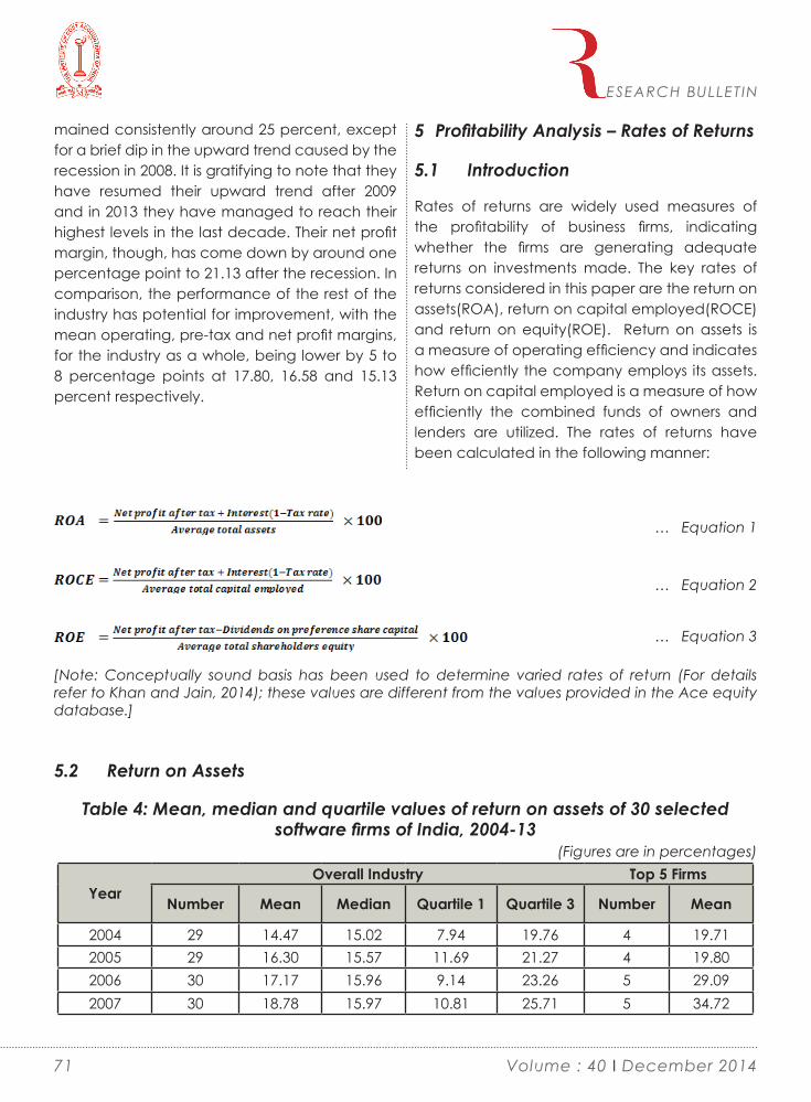
mained consistently around 25 percent, except for a brief dip in the upward trend caused by the recession in 2008. It is gratifying to note that they have resumed their upward trend after 2009 and in 2013 they have managed to reach their highest levels in the last decade. Their net profit margin, though, has come down by around one percentage point to 21.13 after the recession. In comparison, the performance of the rest of the industry has potential for improvement, with the mean operating, pre-tax and net profit margins, for the industry as a whole, being lower by 5 to 8 percentage points at 17.80, 16.58 and 15.13 percent respectively.
5 Profitability Analysis – Rates of Returns
5.1 Introduction
Rates of returns are widely used measures of the profitability of business firms, indicating whether the firms are generating adequate returns on investments made. The key rates of returns considered in this paper are the return on assets(ROA), return on capital employed(ROCE) and return on equity(ROE). Return on assets is a measure of operating efficiency and indicates how efficiently the company employs its assets. Return on capital employed is a measure of how efficiently the combined funds of owners and lenders are utilized. The rates of returns have been calculated in the following manner:
ESEARCH BULLETIN
… Equation 1
… Equation 2
… Equation 3
[Note: Conceptually sound basis has been used to determine varied rates of return (For details refer to Khan and Jain, 2014); these values are different from the values provided in the Ace equity database.]
5.2 Return on Assets
Table 4: Mean, median and quartile values of return on assets of 30 selected software firms of India, 2004-13
(Figures are in percentages)
YearOverall Industry Top 5 Firms
Number Mean Median Quartile 1 Quartile 3 Number Mean
2004 29 14.47 15.02 7.94 19.76 4 19.712005 29 16.30 15.57 11.69 21.27 4 19.802006 30 17.17 15.96 9.14 23.26 5 29.092007 30 18.78 15.97 10.81 25.71 5 34.72
71 Volume : 40 I December 2014

YearOverall Industry Top 5 Firms
Number Mean Median Quartile 1 Quartile 3 Number Mean
2008 30 16.54 15.97 9.43 22.15 5 28.102009 30 15.09 14.15 9.16 20.22 5 25.842010 30 14.60 14.31 8.78 20.11 5 21.072011 30 13.52 13.63 8.30 17.14 5 19.552012 30 12.19 12.22 5.37 16.99 5 20.992013 30 12.98 10.93 6.68 18.50 5 21.48
2004-08 29-30 16.67 15.56 10.01 23.35 4-5 26.852009-13 30 13.68 13.58 7.70 18.82 5 21.792004-13 29-30 15.16 14.34 8.68 20.55 4-5 24.21
Note: Extreme values over +/- 50 percent have been excluded while calculating above table. Source of data – Ace Equity Database
Paired Samples t-Test Paired Differences
t dfSig.(2-tailed)
Between ‘Pre’ and
‘Post’ periods
Mean Std. DeviationStd. Error
Mean
95% Confidence Interval of the Diff
Lower Upper
(2004-08) (2009-13)
-3.31367 7.60591 1.38864 -6.15376 -.47357 -2.386 29 .024
ESEARCH BULLETIN
Table 4 indicates that there has been a drop in the mean ROA for the industry as a whole from 16.67 percent to 13.68 percent between the pre- and post-recession periods. The top 5 firms have seen a steeper fall by nearly 5 percentage points, from 26.85 percent to 21.79 percent. In spite of this decrease, their overall levels have been quite satisfactory in comparison to the industry as a whole, with a mean ROA range of 12.19 – 18.78 percent.
This fall in ROA can be explained due to reduc-tion in growth of sales without commensurate reduction in costs and asset base. We venture to feel that the firms would have retrenched excess contract staff and vacated part of leased office space as well as computer hardware equipment (thereby reducing lease costs), realizing pres-
ence of excess capacity due to the onset of the recession; such measures would have reduced the operating costs.The steeper fall in ROA for the top 5 firms has been, in part, due to build-up of very high levels of cash holdings by these firms during this period. Although such high levels of cash holdings have traditionally been considered as unproductive and an inefficient mode of holding assets, recent literature has hinted that large number of firms, especially in the technology and R&D space have been tending to hold higher levels of cash, as level of risk and investments in R&D have been increasing(Bates, Kahle and Stulz, 2009). Higher cash holdings have been also viewed as a potent tool for enabling proactive, strategic decisions required for checking the growth of
72Volume : 40 I December 2014

competition (Fresard, 2010). One may observe a similar pattern, with a gradual consolidation by the top 5 firms, which have nearly doubled their share of Indian software exports from around 25 percent to over 50 percent between 2004 and 2013, while their cash-to-total assets ratio doubled from 10 percent to 19 percent (Figure 8) during the same period.
Figure 7: Trend of mean cash and bank balances of 30 selected software firms of India, 2004-13
Figure 7 reveals a general upward trend in cash and bank balances of the software industry from year 2005 onwards.
Figure 8: Trend of mean cash to total assets ratio of 30 selected software firms of India, 2004-13
ESEARCH BULLETIN
The trend in Figure 8 indicates that the mean cash-to-total assets ratio for the top 5 firms has almost doubled from 10 percent to 19 percent between 2004 and 2013. In comparison, the mean ratio has remained almost unchanged for the industry as a whole. These observations are in conformity with findings of Kim and Bettis(2013)
that cash holdings of larger firms become more valuable as a strategic competitive resource.
73 Volume : 40 I December 2014

Figure 9: Trend of mean return on assets of 30 selected software firms of India, 2004-13
5.3 Return on Capital Employed
Table 5: Mean, median and quartile values of return on capital employed of 30 selected software firms of India, 2004-13
(Figures are in percentages)
YearOverall Industry Top 5 Firms
Number Mean Median Quartile1 Quartile3 Number Mean2004 29 17.99 18.02 9.69 23.86 4 26.022005 29 20.87 19.52 15.49 26.58 4 26.70
2006 30 22.78 21.31 11.19 31.11 5 39.882007 29 23.14 19.38 12.98 35.58 4 42.212008 30 22.65 19.81 10.62 33.01 5 40.292009 29 19.27 18.55 10.22 26.53 5 36.902010 30 19.28 18.94 10.54 25.30 5 28.08
2011 30 17.50 17.76 10.09 21.74 5 25.522012 30 16.14 16.57 6.68 22.91 5 27.842013 29 16.05 14.53 7.95 23.90 5 29.33
2004-08 29-30 21.50 19.38 11.66 30.22 4-5 35.482009-13 29-30 17.64 17.21 9.31 24.58 5 29.54
2004-13 29-30 19.57 18.55 10.13 26.36 4-5 32.32
Note: Extreme values over +/- 75 percent have been excluded while calculating above table. Source of data – Ace Equity Database
ESEARCH BULLETIN
Figure 9 reveals that that the return on assets of the top 5 software firms of India has been con-sistently higher, nearly one and a half times that of the industry as a whole. This indicates that the top 5 firms have been able to utilize their assets
better. The top 5 firms had witnessed a sharp in-crease in the ROA in years 2006 and 2007, which slowly got reduced to its previous levels after the recession.
74Volume : 40 I December 2014

Paired Samples t-Test Paired Differences
t dfSig.(2-tailed)
Between ‘Pre’ and
‘Post’ periods
Mean Std. Deviation
Std. Error Mean
95% Confidence Interval of the Diff
Lower Upper
(2004-08) - (2009-
13)-4.35833 9.94479 1.81566 -8.07178 -.64489 -2.400 29 .023
ESEARCH BULLETIN
Table 5 indicates that there has been a reduc-tion in mean value of ROCE for the industry as a whole by around 4 percentage points from 21.50 percent to 17.64 percent. The mean value of ROCE for the top 5 firms continues to demon-strate a robust figure of 29.54 percent even after a steep fall of around 6 percentage points. The results of the t-test are in line with this, indicating that there has been a significant impact on the means of the ROCE. The fall in the ROCE has been observed to be higher for the top 5 firms, in comparison to the industry as a whole. This could
partly be explained by the fact that the bigger firms in the industry had a build-up of liquid assets of cash and bank balances on the higher side. In the absence of expansionary needs, the industry could have used these funds to retire whatever little debt it had, or paid back higher amounts to its shareholders in the form of dividends and share buybacks. However, it seems that the industry chose to retain the capital for future needs/expansion.
Figure 10: Trend of mean return on capital employed of 30 selected software firms of India, 2004-13
Figure 10 shows that the mean ROCE values rose marginally in 2006 and 2007, for the industry as a whole; in subsequent years it had a downward trend till 2013. The top 5 firms had also seen a significant jump in mean ROCE values between 2006 and 2008. This gradually fell back to the original levels by 2011. The top 5 firms broadly
delivered an ROCE of more than one and half times that of the industry as a whole.
75 Volume : 40 I December 2014

ESEARCH BULLETIN
5.4 Return on Equity
Table 6: Mean, median and quartile values of return on equity of 30 selected software firms of India, 2004-13
(Figures are in percentages)
YearOverall Industry Top 5 Firms
Number Mean Median Quartile1 Quartile3 Number Mean2004 28 18.91 18.15 12.55 27.36 4 26.182005 29 21.51 21.06 15.49 28.27 4 26.912006 29 22.45 21.54 13.38 29.95 5 40.132007 29 24.40 20.95 12.99 36.09 4 42.402008 30 22.86 21.50 11.11 28.92 5 41.812009 30 20.73 20.53 10.94 29.34 5 38.692010 30 20.87 20.85 12.05 30.38 5 31.412011 30 18.27 19.73 10.37 23.11 5 28.162012 30 15.33 17.37 6.65 23.21 5 29.282013 29 14.77 15.12 7.94 23.91 5 31.22
2004-08 28-30 22.05 20.68 12.99 29.95 4-5 35.982009-13 29-30 18.02 18.37 9.32 26.32 5 31.752004-13 28-30 20.01 19.35 10.80 27.84 4-5 33.73
Note: Extreme values over +/- 75 percent have been excluded while calculating above table. Source of data – Ace Equity Database
Paired Samples t-Test Paired Differences
t dfSig.(2-tailed)
Between ‘Pre’ and
‘Post’ periods
Mean Std. Deviation Std. Error Mean
95% Confidence Interval of the Diff
Lower Upper
(2004-08) - (2009-
13)-4.65500 10.78049 1.96824 -8.68050 -.62950 -2.365 29 .025
The results in Table 6 reveal that after the re-cession the ROE values dipped by around 4 percentage points for all segments of the indus-try. The mean of the return on equity for the top 5 firms remained more than satisfactory in spite of falling from 35.98 percent in the pre-recessionary
phase to 31.75 percent in the post-recessionary phase. The industry as a whole, in comparison, showed average performance, with the mean return on equity falling from 22.05 percent to 18.02 percent after the recession. The results of the t-test confirm that there has been a signifi-cant impact of recession on the ROE.
76Volume : 40 I December 2014

Figure 11: Trend of mean return on equity of 30 selected software firms of India, 2004-13
ESEARCH BULLETIN
Figure 11 reveals that the return on equity of the top 5 firms is consistently higher than the industry average, by and large, yielding a return on eq-uity of more than one and a half to twice that of the industry average. Before the recession, the ROE for the industry as a whole was stable, although the top 5 firms showed a consistent rise in ROE between 2005 and 2007. After the reces-sion, the ROE had come off the peak values by nearly one third, for all segments of the industry. The top 5 firms have shown an upward trend in ROE from 2012 onwards.
In sum, the analysis of the rates of returns of the Indian software industry has revealed that in marked contrast with the profit margins, there has been an almost secular reduction in the val-ues of the ROA, ROCE and ROE, for all segments of the industry, ranging between 1 to 6 percent-age points, after the recession. The t-tests reveal that there has been a significant difference in the means of all three rates of returns between the pre- and post-recession periods. The results have been cross-validated using the Wilcoxon paired signed rank test.The top 5 firms have been impacted to a higher extent, partly due to build-up of non-productive cash-assets. In spite of a higher fall in the ratios for the top 5 firms, their mean rates of returns have been quite sat-isfactory, giving nearly one and a half times the returns of the industry as a whole.
6 DuPont Analysis
6.1 Introduction
The objective of this section is to assess profit-ability performance of Indian software industry using DuPont Analysis. DuPont analysis enables to view how the ROE is affected by the operat-ing, investing and financing decisions of a firm, represented by:
►► operating efficiency, which is measured by the net profit margin,
►► asset use efficiency, which is measured by total assets turnover ratio and
►► financial leverage, which is measured by the equity multiplier.
… Equation 4
77 Volume : 40 I December 2014

6.2 3-Component DuPont Analysis
Table 7: Mean and median values of DuPontelements of 30 selected software firms of India, 2004-13
(Figures are in ratios)
Year Net Profit Margin Assets Turnover Ratio Equity Multiplier ROE
Mean Median Mean Median Mean Median Mean Median2003-04 0.19 0.17 1.10 0.98 1.37 1.28 0.22 0.20
2004-05 0.17 0.17 1.24 1.19 1.83 1.32 0.30 0.22
2005-06 0.18 0.17 1.03 0.93 1.52 1.36 0.25 0.24
2006-07 0.18 0.16 1.11 0.99 1.89 1.41 0.33 0.22
2007-08 0.17 0.17 1.05 1.03 1.58 1.39 0.25 0.23
2008-09 0.16 0.14 1.13 1.06 1.62 1.36 0.24 0.22
2009-10 0.16 0.17 0.96 0.87 1.67 1.42 0.22 0.24
2010-11 0.17 0.15 0.90 0.82 1.57 1.32 0.19 0.21
2011-12 0.13 0.11 1.00 0.86 1.54 1.36 0.18 0.17
2012-13 0.13 0.14 0.99 0.89 1.77 1.36 0.19 0.15
Source of data – Ace Equity Database
Table 7 lists the year-wise means of the various ratios under the 3-component DuPont analysis. Figure 12 is a plot of these figures, showing how these ratios varied over time.
Figure 12: Trend of mean DuPont elements of 30 selected software firms of India, 2004-13
ESEARCH BULLETIN
78Volume : 40 I December 2014

A regression analysis was carried out for the ROE using the 3-component DuPont equation.
... Equation 5
Table 8: Results of regression analysis on DuPont equation based on 30 selected software firms of India, 2004-13
Summary Output
Regression StatisticsMultiple R 0.859587905R Square 0.738891367Audjusted R Square 0.735654483Standard Error 0.093601425Observations 246
ANOVAdf ss MS F Significance F
Regression 3 5.999839697 1.999946566 228.2724352 2.92063E-70Residual 242 2.120216874 0.008761227Total 245 8.120056571
Coefficients Standard Error t Stat P-value Lower 95% Upper 95%
Intercept -0.30554324 0.02189202 -13.95683189 7.09635E-33 -0.348666472 -0.262420008
NPM 1.192374698 0.066468006 17.93907725 2.42421E-46 1.061445014 1.323304383Asset Turnover
0.212408706 0.010620223 20.00040009 3.46624E-53 0.19148883 0.233328581
Equity Multiplier
0.07676388 0.006038597 12.71220543 1.06478E-28 0.064868961 0.088658798
ESEARCH BULLETIN
79
It is worth mentioning that the regression results can be relied for interpretation as the statistical analysis in terms of correlation between the in-dependent variables and autocorrelation in the dependent variable has been carried out. The correlation analysis does not suggest a strong correlation between the independent variables. Likewise, the results indicate that the autocor-relation coefficient lies well within the critical
range, for a vast majority of the firms, thereby suggesting that we may assume absence of strong auto-correlation in the dependent vari-able.
Volume : 40 I December 2014

Table 9 : Correlation coefficients among the independent variables
Net Profit Margin Assets Turnover Equity Multiplier
Net Profit Margin 1
Assets Turnover -0.28 1
Equity Multiplier -0.24 0.10 1
Figure 13: Firm-wise first-order autocorrelation coefficients for ROE
ESEARCH BULLETIN
The adjusted R-square value of 0.7356 in Table 8 indicates that more than 73 percent of the cases can be explained well with the help of the equation. The significance value of F-test and the P-values for the individual coefficients
are less than 0.05 and therefore indicate that the results are significant and can be accepted. Based on the results shown above, the regression equation can be written as
80
… Equation 6
Equation 6 reveals that a unit change in net profit margin would lead to a change of 1.192 times in ROE; a unit change in assets turnover ratio would lead to a change of 0.212 times in ROE; the last is the equity multiplier ratio which has a multiplier effect of only 0.077. The recommendation for the industry is that it should focus on improving its net profit margin and assets turnover ratio as the greatest improvement in ROE can be achieved
by improving these two ratios.
In order to improve their net profit margins, firms would need to work at improving their oper-ational costs. In addition, small and mid-sized firms, which have sizeable interest burden, could benefit significantly by retiring debt and reduc-ing this interest component.
One of the factors which firms could turn in their
Volume : 40 I December 2014
favor is the assets turnover ratio. The firms should make all efforts to identify outlets of utilizing their idle cash and bank balances in a better manner, increasing the overall productivity of their assets. They could also look into introducing multiple shift work in their offices. This would result in increased sales, without commensurate increase in fixed assets base. This is something which is routinely followed by the IT enabled services sector.
7 Concluding Observations
The study indicates that in spite of the global slowdown and major spending cuts in IT budgets of firms across USA and Europe, the software firms of India have managed to remain profitable, although there was a temporary dip in the mar-gins in 2009. There was no significant impact of the global slowdown on the operating, pre-tax and net profit margins of the industry as a whole, which reduced by only 1 percentage point af-ter the recession. The fall in the margins was to some extent cushioned by the depreciation of the rupee against the major foreign currencies during this period. The top 5 software firms have consistently shown robust operating and pre-tax profit margins of around 25 percent and net profit margin of around 22 percent. In comparison, the profit margins for the industry as a whole, based on the 10 year period of the study, have been found to be lower by 6 to 8 percentage points.
It has been observed that there has also been a marked difference in the rates of returns of the top 5 firms, compared to the rest of the industry. The top 5 firms earned nearly one and a half times the returns which the industry as a whole yielded. After the recession, there has been an almost secular reduction in the values of the ROA, ROCE and ROE, for all segments of the industry, ranging between 1 to 6 percentage points. The top 5 firms have been impacted to a higher extent, partly due to steep build-up of non-productive assets in the form of cash and
bank balances.
During the period of study, the top 5 firms have managed to squeeze out competition, and increased their market share from around 25 per-cent to over 50 percent of total software exports from India. It has been observed that this has coincided with a near doubling in cash-to-assets ratio of the top 5 firms during the same period, substantiating earlier research which hints at a correlation between high cash levels and ability to make proactive, strategic moves to stifle the growth of competition.
The recommendation for the industry, based on the DuPont analysis and the regression carried out, is to focus foremost on improving the net profit margin and the assets turnover ratio. Small and mid-sized firms, having a sizeable interest burden, could benefit significantly by retiring debt and reducing this burden. Other firms can look into reducing their idle cash holdings and improving the overall productivity of their assets, by either paying back the shareholders in the form of dividends or buy back of shares, or using them for making strategic investments for future growth. They could also introduce multiple shift work in their offices, resulting in increased sales, without commensurate increase in fixed assets base.
Overall, in spite of the global downturn, the Indi-an software industry has been able to maintain financial ratios within a healthy range, compared to other industries. This has been partly because its value proposition continues to be relevant, perhaps becoming even more compelling, in the wake of the global recession, where global clients are forced to rethink on ways to reduce their costs. However, the industry needs to learn lessons from its peers like Ireland and Israel and needs to move up the value chain, increasing its revenue per employee to a much higher level by offering innovations and products to the global market, rather than just remaining a services
ESEARCH BULLETIN
81 Volume : 40 I December 2014

oriented industry. It also needs to take inspiration from China and Brazil and grow the domestic market divisions, failing which this market is likely to be captured by the foreign competition.
References
Arora, A. and Gambardella, A. (2004). “The globalization of the software industry: perspectives and opportunities for developed and developing countries” (No. w10538). Na-tional Bureau of Economic Research.
Arora, A. and Gambardela , A.(2005), “From underdogs to tigers - The rise and growth of the software industry in Brazil, China, India, Ire-land and Israel” , Oxford University Press.
Bates, T. W., Kahle, K. M. and Stulz, R. M. (2009). “Why do US firms hold so much more cash than they used to?”, The Journal of Finance, 64(5), 1985-2021.
Bhatnagar, S. (2006). “India’s software industry.” In Chandra, V. (Ed.), Technology, ad-aptation and exports: How some developing countries got it right (pp 49-81). World Bank Pub-lications.
Government of India, Ministry of Fi-nance(2014). “Economic Survey 2013-14.”
Forbes India (2013, July), “Will Business Restructuring Fuel Polaris Financial Technology’s Growth?”, Retrieved from http://forbesindia.com/article/big-bet/will-business-restructuring-fu-el-polaris-financial-technologys-growth/35653/2
Fresard, L. (2010). “Financial strength and product market behavior: The real effects of cor-porate cash holdings.”, The Journal of finance, 65(3), 1097-1122.
Ghosh, J. and Chandrasekhar, C. P. (2009). “The costs of ‘coupling’: The global crisis and the Indian economy”, Cambridge Journal of Economics, 33(4), 725-739.
India Brand Equity Foundation(2014). “IT and ITeS.” Retrieved from http://www.ibef.org/download/IT-and-ITeS-March-2014.pdf
UNCTAD(2012). “Information Economy Report 2012.” Retrieved from http://www.unct-ad.org/en/PublicationsLibrary/ier2012_en.pdf
Khan, M. Y. and Jain, P. K. (2014). ’’Finan-cial management: Text, problems and cases”, McGraw Hill, New Delhi.
Kim, C., and Bettis, R. A. (2013). “Cash is surprisingly valuable as a strategic asset.”, Strate-gic Management Journal. doi: 10.1002/smj.2205
Kumar, Rajiv; Vashisht, Pankaj (2009) : “The global economic crisis: Impact on India and policy responses”, Asian Development Bank Institute working paper series 164. Tokyo: ADB In-stitute.
Zhou, J. (2009). “Increase in Cash Hold-ings: Pervasive or Sector-Specific?”, University of Toronto[Online]. Retrieved from:
http://69.175.2.130/~finman/Reno/Pa-pers/increaseincashholdings_Jan152009_fma09.pdf
ESEARCH BULLETIN
82Volume : 40 I December 2014

Foreign Direct Investment in Indian Scenario: An Empirical Study of Service Sector
Arindam BanerjeeAbstract
Service sector is one of the fastest growing sectors in India. It contribution to Indian economy has been manifold which is about 55.2% in Gross Domestic Product and is growing by 10% annually. One of the important things observed is that the share of Service sector in total Foreign Direct Investment in India has increased by leaps and bound in the few past years. One of the important observations that can be made is that during 1991 to 2005 the share of service sector in Total FDI in Indian Economy was just 9.76% occupying 5th position, but its share in total FDI has increased to around 21% occupying the 1st position in 2011 as per the report available through DIPP website.
Keywords
FDI, Power, Investment, Inflows, Government
importance of foreign capital’s role in the rapid industrial and economic development. It contrib-utes a lot to the economic growth and industrial development across the world. It even acts as a catalyst in the process of domestic industrial development. Further it helps in speeding up economic activity and brings with it other scarce productive factors such as technical know- how and managerial experience, which are essential for economic development.
FDI plays an important role in the development process of a country. It has potential for making contribution to the economic development through the transfer of financial resources, tech-nology innovation and improved management techniques. Developing countries like India need substantial foreign inflows to achieve the required investment to accelerate economic growth and development.
1.1 Meaning of FDI
FDI is generally defined as “A form of long term international capital movement made for the purpose of productivity activity and accompa-nied by the intention of managerial control or participation in the management of the foreign firm”.
According to the International monetary fund, FDI can be defined as “An Investment that is made to acquire a lasting interest in an enter-prise operating in an economy other than that of the investor. The investor’s purpose is to have an effective voice in the management of the enter-
ESEARCH BULLETIN
83
1. Introduction
In the 21st century India is an emerging econom-ic power with vast human and natural resources and a huge knowledge base. The economy of India is the twelfth largest economy in the world by nominal value and the fourth largest by Pur-chasing Power Parity (PPP).
Foreign Direct Investment (FDI) has been in-creasing dramatically across the world. Almost all the countries in the world are realizing the
Volume : 40 I December 2014

prise.” FDI should not be confused with portfolio investment, which doesn’t seek management control. Portfolio investment occurs when an individual investor invest, mostly through stock-brokers in the stocks of the foreign countries in search of profit opportunities.
The World Investment Report of the United Na-tions Conference on trade and development (UNCTAD) defines FDI as “International Invest-ment that reflects the objective of a resident entity in one economy (Foreign Direct Investor or Parent Enterprise) obtaining “Lasting Interest” in and control of an enterprise resident in a economy other than that of foreign direct inves-tor.” Lasting interest implies the existence of a long-term relationship between a direct investor and the enterprise and a significant degree of influence on the management of the enterprise.
1.2 The Service Sector in India
Service sector is one of the fastest growing sectors in India. It contribution to Indian econo-my has been manifold which is about 55.2% in Gross Domestic Product and is growing by 10% annually. One of the important things observed in share of Service sector in total Foreign Direct Investment in India is that it has increased by leaps and bound in the few past years.
One of the important observations that can be made is that during 1991 to 2005 the share of ser-vice sector in Total FDI was just 9.76% occupying 5th position, but its share in total FDI has increased to around 21% occupying the 1st position in 2011 as per the report available through DIPP website.
1.3 FDI Policy in relation to the Service Sector In this paper an attempt has been made to analyze the FDI Inflows in Service Sector (both Financial and Non Financial) as well as compo-nent wise like Telecommunication, Hotel and
Tourism etc. Some of the FDI policies in relation to different service sector are given below:
Example in Insurance Sector, FDI is allowed on the automatic route subject to obtaining license from Insurance Regulatory &Development Au-thority (IRDA).In private Sector Banking, FDI of 49% from all sources on the automatic route is allowed subject to guidelines issued from RBI. In telecommunication Industry, FDI is limited to 49% subject to licensing and security requirements and adherence by the companies. In trading, FDI up to 51% is allowed provided that it is pri-marily export activities, and the undertaking is an export house/trading house/super trading house. 2. Objective of the Study The study primarily focuses on the following ob-jectives:
a. Analysis of overall Sectoral FDI inflows in India from 2002 to 2011.
b. Analysis of the FDI Inflows in Service Sector from 2000 to 2011.
c. Analysis of monthly FDI Inflows in Service Sector in 2009-10 and 2010-11.
d. Analysis of Component Wise break up of FDI Inflow in Service Sector in India.
3. Literature Review
It is proposed to present briefly some of the litera-tures referred by me while conducting the study.
► Liesbeth Colen, Miet Maertens, Jo Swinnen (2008) has worked on “FDI as an Engine for Economic Growth and Human Development. The objective of the study was to analyze the importance of FDI on developing countries with a view to highlight the trend of the FDI flows. The study further tries to evaluate the effect of FDI on
ESEARCH BULLETIN
84Volume : 40 I December 2014
economic growth as well as poverty reduction.
► Mahima Dass Gupta (2005) aims at ana-lyzing the role and performance of FDI in India. This study focuses on analyzing different routes through which FDI comes to India or the dimen-sion and trend of FDI vis a vis certain selected Asian countries.
► Dr. H. A. C. Prasad and R. Sathish (2010) in their working Paper (Department of Economic Affairs Ministry of Finance Government of India) titled ‘Policy for India’s Services Sector’ have examined major issues concerning India’s service sector. They have given both general and sector specific policy suggestion. The paper also emphasizes on the importance of services for India in terms of GDP growth, services export growth and openness of the economy.
► M. Selvakumar, T. Ambika and S. Muthu-lakshmi (2007) in their article “Foreign Direct Investment in Service Sector” have focused on trend and pattern of FDI in Indian Service Sector and the Global trend of FDI in Service Sector and emphasizes that efforts should be made to-wards attracting efficiency seeking FDI through a right policy that expand operation, improve local skills, establish linkages and upgrade tech-nology.
► Mahima Dass Gupta (2005) aims at ana-lyzing the role and performance of FDI in India. This study focuses on analyzing different routes through which FDI comes to India or the dimen-sion and trend of FDI vis a vis certain selected Asian countries.
► Economic Survey (2010-11) emphasized that India stands out for the size and dynamism of its service sectors. The contribution of Service sector to the Indian Economy has been man-ifold. It highlights various aspects of Service Sector like sectors attracting highest FDI Inflows in India (Service sector occupying the top posi-tion), Service Exports, share of different service categories in GDP, share and growth of Service
sector etc.
4. Research Methodology
The data relevant to the study has been col-lected from various sources like the report of the ministry of commerce and industry, the depart-ment of Industrial promotion and policy (DIPP), the government of India, Centre of Monitoring Indian Economy (CMIE), Reserve Bank of India, and Journals. Various information has also been taken from World development reports and World Investment Reports. The data has been analyzed by using statistical tools like correlation, simple regression model (using least square method) so as to draw valid conclusion. SPSS 16 has been used for analysis purpose apart from other statistical analysis with graphs etc.
5. Analysis
The entire analysis for the study has been con-ducted in different sections as discussed below:
5.1 : This section basically deals with the distribu-tion of the FDI Inflows in different sectors in Indian Economy.
Table 1 deals with the FDI Inflows in top 5 sectors in Indian Economy. It is observed from Table 1 that Service sector (comprising of financial and non financial) attracts the maximum FDI Inflows in Indian economy i.e. 26835US $(in millions)from 2002 to 2011. Service sector is followed by Computer software and Hardware , Tele-communication, House and Real Estate and Construction in terms of attracting the maximum FDI inflows in Indian economy from 2002 to 2011.
The result of Table 1 is produced below:
ESEARCH BULLETIN
85 Volume : 40 I December 2014

Table 1 : Top 5 sectors attracting the maximum FDI Inflow in Indian Economy
Sector 2002-03
2003-04
2004-05
2005-06
2006-07
2007-08
2008-09
2009-10
2010-11 Total
Service Sector (Financial and Non Financial)
326 269 469 581 4664 6615 6116 4392 3403 26835
Computer Hard & Soft 644 532 721 1451 2733 1410 1677 919 484 10571Telecom 223 116 129 686 521 1261 2558 2554 1665 9713Real estate N.A N.A N.A 38 467 2179 2801 2844 1127 9456Construction 21 47 152 151 985 1743 2028 2868 1125 9120
Source: Website of Department of Industrial promotion and policy (DIPP), In the table : N.A Means Not Available and amount are expressed in US $ (in millions)
Thus we can observe from Section 5.1 that Service Sector occupies 1st position among the sectors having the maximum FDI Inflows in Indian Scenario from 2002 to 2010.
5.2 : This section deals with percentage of FDI Inflows to total cumulative FDI inflows of Indian economy for Top 5 sectors in Indian scenario. It was observed from the previous section that ser-vice sector attracted the maximum FDI Inflows in Indian Economy.
Table 2 deals with the percentage of FDI inflows to Total cumulative FDI inflows in Indian econo-my for Top 5 sectors. It is observed from Table 2 that percentage of FDI Inflows to cumulative FDI inflows is maximum for Service sector (20.82%) followed by Computer Software and Hardware , Telecommunication, House and Real Estate and Construction from 2000 to 2011.
The result of Table 2 is produced below:
ESEARCH BULLETIN
Table 2. Percentage of FDI Inflows to cumulative FDI Inflows for top 5 Sectors
Amount Expressed in US $ (in millions)
Total Cumulative Inflow % Inflows
Service Sector(Financial and Non Financial) 27007 20. 82
Computer Software and Hardware 10723
8.26
Telecommunication 10589 8.16
House and Real Estate 9632 7.42
Construction 9178 7.07
86Volume : 40 I December 2014

Total Cumulative Inflow % Inflows
Cumulative Inflow (2000 to 2011) 129716
Source: Website of Department of Industrial promotion and policy (DIPP)
ESEARCH BULLETIN
Thus we can observe from Section 5.2 that the percentage of FDI Inflows to Total cumulative FDI Inflows is maximum for service sector in Indian scenario from 2000 to 2010.
5.3 : In this section an attempt has been made to further investigate the percentage of FDI Inflows in Service sector to Total cumulative FDI Inflows in Indian Economy from 2002 to 2010.
Table 3 deals with the above objective. It is ob-
served from Table 3 that the percentage of FDI Inflow in the Service sector to the cumulative FDI inflow in Indian economy is maximum in the year 2006-07 (29.6%) followed by 2007-08 and 2008-09. The total percentage of FDI Inflow in Service sector to the total FDI Inflow in Indian Economy from 2002-03 to 2009-10 is 21.5%. This makes service sector holds a prominent (1st) position among different sectors attracting FDI inflows.
The result of Table 3 is produced below:
Table 3:Cumulative FDI Inflow Indian Economy Vs FDI Inflows in Service Sector
Amount Expressed in US $ (in millions)
Year Cumulative FDI Inflows
FDI Inflows in Service Sector (Financial and Non Financial) % of FDI Inflows
2002-03 3134 326 10.42003-04 2634 269 10.22004-05 3755 469 12.52005-06 5549 581 10.42006-07 15730 4664 29.62007-08 24579 6615 26.92008-09 27309 6138 22.42009-10 25888 4353 16.8Total 108578 23415 21.5
Source: Website of Department of Industrial promotion and policy (DIPP)
87
5.4: It has been an endeavor in this section to investigate into the relationship between Cumu-lative FDI in Indian Economy and FDI in Service Sector through correlation and regression analy-sis. SPSS 16 is used for analysis purpose.
Table 4 is basically dealing with the correlation
between Cumulative FDI in Indian Economy and FDI in Service Sector. It is observed from Table 4 that correlation is .952 which is depicting a very high positive correlation.
The result of correlation matrix is produced in Table 4:
Volume : 40 I December 2014

Table 4 (Correlation Matrix)
CorrelationsCum.FDI FDI.Service
Cum.FDIPearson Correlation 1.000 .952**
Sig. (2-tailed) .000N 8.000 8
FDI.ServicePearson Correlation .952** 1.000Sig. (2-tailed) .000N 8 8.000
**. Correlation is significant at the 0.01 level (2-tailed).
The significant influence of FDI in Service Sector on the Total Cumulative FDI in Indian Economy is further tested by Regression analysis using SPSS 16.
Table 5 consists of the regression results. Cumula-tive FDI is taken as a dependent variable and FDI inflow in service sector is taken as independent variable for the study. It is observed from Table
5 that R square is .906 meaning that 90.6% of the Cumulative FDI in India Economy is explained by FDI in Service Sector. The result of Table 5 is produced below:
Table 5 (Regression Results:R2)
Model Summary
Model R R Square Adjusted R Square
Std. Error of the Estimate
1 .952a .906 .890 3667.64246
a. Predictors: (Constant), FDI.SERVICE
ESEARCH BULLETIN
Table 6 basically investigates into the significant influence of FDI inflows in service sector on the cumulative FDI Inflows in Indian Economy. It is ob-served from Table 6 that t value of FDI in Service Sector is 7.590 (which is beyond the range of - 2 and +2) and p value of .000 (p < .05). Hence the
FDI in Service Sector is a very significant factor in-fluencing the Cumulative FDI in Indian Economy. The beta coefficient is positive indicating that FDI in Service Sector is positively influencing the Cumulative FDI in Indian Economy. The result of Table 6 is produced below.
88
Table 6: Regression Results
ModelUnstandardized
CoefficientsStandardized Coefficients t Sig.
B Std. Error Beta
1(Constant) 2519.934 1949.908 1.292 .244FDI.Service 3.776 .498 .952 7.590 .000
a. Dependent Variable: Cum.FDI
Volume : 40 I December 2014

We can plot a graph between Cumulative FDI Inflows and FDI Inflows in Service Sector (refer table 3) as shown below:
Graph 1 : Cumulative FDI Inflows and FDI Inflows in Service Sector
X-axis: years, Y axis: FDI Inflows, Series 1: Cumulative FDI Inflows, Series 2: FDI Inflows in Service Sector
ESEARCH BULLETIN
It can observed from the above graph that the FDI inflow in Service sector has increased with the increase of total FDI Inflows in India. But FDI inflow in Service sector has decreased with the decrease of total FDI Inflows in India in the year 2009-10 which is again reflecting a very positive correlation.
5.5 : This section deals with graphical representa-tion of the FDI inflows in Service sector from 2002 to 2010.
Graph 1 reflects the FDI Inflows in Service Sector in Indian Scenario from 2002-03 to 2009-10.
It is observed from graph 1 that the highest FDI Inflows in Service Sector was in the year 2007-08 (6615 US $ (in millions)) followed by the year 2008-09 and 2006-07.
So, a steady increase in the FDI Inflows in the service sector is observed though it has reduced a bit in the year 2009-10 compared to 2008-09.
The graph 2 is produced below:
89 Volume : 40 I December 2014
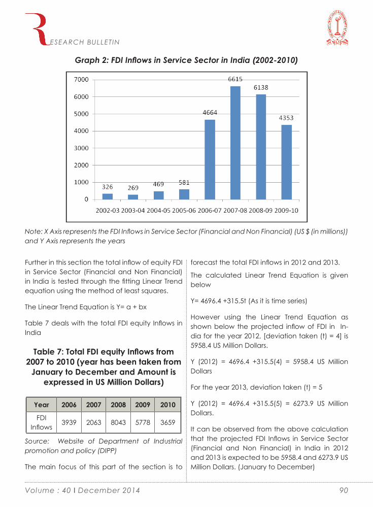
Graph 2: FDI Inflows in Service Sector in India (2002-2010)
Note: X Axis represents the FDI Inflows in Service Sector (Financial and Non Financial) (US $ (in millions)) and Y Axis represents the years
Further in this section the total inflow of equity FDI in Service Sector (Financial and Non Financial) in India is tested through the fitting Linear Trend equation using the method of least squares.
The Linear Trend Equation is Y= a + bx
Table 7 deals with the total FDI equity Inflows in India
Table 7: Total FDI equity Inflows from 2007 to 2010 (year has been taken from
January to December and Amount is expressed in US Million Dollars)
Year 2006 2007 2008 2009 2010
FDI Inflows
3939 2063 8043 5778 3659
Source: Website of Department of Industrial promotion and policy (DIPP)
The main focus of this part of the section is to
forecast the total FDI inflows in 2012 and 2013.
The calculated Linear Trend Equation is given below
Y= 4696.4 +315.5t (As it is time series)
However using the Linear Trend Equation as shown below the projected inflow of FDI in In-dia for the year 2012, [deviation taken (t) = 4] is 5958.4 US Million Dollars.
Y (2012) = 4696.4 +315.5(4) = 5958.4 US Million Dollars
For the year 2013, deviation taken (t) = 5
Y (2012) = 4696.4 +315.5(5) = 6273.9 US Million Dollars.
It can be observed from the above calculation that the projected FDI Inflows in Service Sector (Financial and Non Financial) in India in 2012 and 2013 is expected to be 5958.4 and 6273.9 US Million Dollars. (January to December)
ESEARCH BULLETIN
90Volume : 40 I December 2014

At the “Focus India Show” in Chicago Indian Commerce and Industry Minister Mr. Kamal Nath told the US investors that India has emerged as the “Best Destination” for FDI and joint ventures. He also described India economy as “India: The Fastest Growing Free Market Democracy”.
5.6: The present section deals with the analysis of monthly FDI Inflow in Service Sector (both Finan-cial and Non Financial) and in India Economy from 2009-10 and 2010-11.
Table 8 reflects the monthly FDI inflows in Indian Economy from 2009 -10 to 2010-11. It is observed from table 8 that during 3 months : May, Sept
and December the increase in FDI Inflows in 2010-11 compared to 2009-10 shows a positive increase of 118, 606 and 472 US $ (in millions) representing 5%,40% and 30% increase.In other months FDI Inflow shows a decreasing trend in 2010-11 compared to 2009-10 , highest being in the month of August of 1938 US $ (in millions) ( representing 59%)If we investigate into the overall FDI Inflow in Indian Economy in 2010-11 compared to 2009-10 we can observe a de-creasing trend. (Absolute decrease 6420 US $ (in millions) representing 24%).
The result of Table 8 is given below:
Table 8: Monthly FDI Equity inflow for the Indian Economy
Month 2009-10 2010-11 Absolute Increase/ Decrease
% Increase/ Decrease
April 2339 2179 -160 -0.068405301
May 2095 2213 118 0.056324582
June 2582 1380 -1202 -0.465530596
July 3476 1785 -1691 -0.486478711
August 3268 1330 -1938 -0.593023256
Sept 1512 2118 606 0.400793651
October 2332 1392 -940 -0.403087479
November 1735 1628 -107 -0.06167147
December 1542 2014 472 0.306095979
January 2042 1042 -1000 -0.489715965
February 1717 1274 -443 -0.258008154
March 1209 1074 -135 -0.111662531Total 25849 19429 -6420 -0.248365507
Source: Website of Department of Industrial promotion and policy (DIPP)
ESEARCH BULLETIN
Table 9 reflects the monthly FDI inflows in Indian service sector from 2009 -10 to 2010-11.
It can be observed from Table 9 that service sector in India is showing a positive increase in the month of July (34%), September (447%), November (36%) and December (135%) for the
year 2010-11 compared to 2009-10. The maxi-mum decrease is reflected in the month of June (-91%) and October (-80%) for the year 2010-11 compared to 2009-10.
The result of Table 9 is produced below:
91 Volume : 40 I December 2014

Table 9 :Monthly FDI inflow in the Indian Service Sector
Month 2009-10 2010-11 Absolute Increase/ Decrease
% Increase/ Decrease
April 655.19 355.25 -299.94 -0.45779087May 492.62 231.83 -260.79 -0.529393853June 781.77 68.45 -713.32 -0.912442278July 286.5 384.2 97.7 0.341012216August 338.52 181.51 -157.01 -0.463813069Sept 147.33 806.09 658.76 4.471322881October 493.53 96.01 -397.52 -0.805462687November 317.46 433.64 116.18 0.365967366December 108.96 256.77 147.81 1.356552863January 330.14 143.27 -186.87 -0.566032592February 307.9 275.2 -32.7 -0.106203313March 207.29 134.6 -72.69 -0.350668146 Total 4467.21 3366.82 -1100.39 -0.246326007
5.7 : The present section investigates the per-centage of FDI Inflow in service sector related to the cumulative FDI Inflow in Indian economy on monthly basis.
Table 10 displays the percentage of FDI Inflow in service sector related to the cumulative FDI Inflow in Indian economy on monthly basis for 2009-10 and 2010-11.
It can be observed from table 10 that in 2009-10, the total FDI Inflow in Indian Service Sector was 17% of the total FDI Inflow in Indian Economy. In the month of June,2009 the percentage of total FDI Inflows in Service sector to the Total FDI Inflows in Indian Economy was the highest (30%) and was the lowest (7%) in December, 2009.
It is further observed from the table that in 2010-11, the total FDI Inflow in Indian Service Sector was again 17% of the total FDI Inflow in Indian Economy. In the month of September, 2010, the percentage of total FDI Inflows in Service sector
to the Total FDI Inflows in Indian Economy was the highest (38%) and was the lowest (5%) in the month of June, 2010.
The result of Table 10 is displayed below.
ESEARCH BULLETIN
92Volume : 40 I December 2014
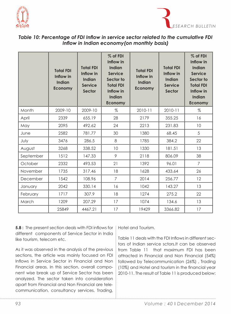
Table 10: Percentage of FDI Inflow in service sector related to the cumulative FDI Inflow in Indian economy(on monthly basis)
Total FDI Inflow in Indian
Economy
Total FDI Inflow in Indian Service Sector
% of FDI Inflow in Indian Service
Sector to Total FDI Inflow in Indian
Economy
Total FDI Inflow in Indian
Economy
Total FDI Inflow in Indian Service Sector
% of FDI Inflow in Indian Service
Sector to Total FDI Inflow in Indian
Economy
Month 2009-10 2009-10 % 2010-11 2010-11 %
April 2339 655.19 28 2179 355.25 16
May 2095 492.62 24 2213 231.83 10
June 2582 781.77 30 1380 68.45 5
July 3476 286.5 8 1785 384.2 22
August 3268 338.52 10 1330 181.51 13
September 1512 147.33 9 2118 806.09 38
October 2332 493.53 21 1392 96.01 7
November 1735 317.46 18 1628 433.64 26
December 1542 108.96 7 2014 256.77 12
January 2042 330.14 16 1042 143.27 13
February 1717 307.9 18 1274 275.2 22
March 1209 207.29 17 1074 134.6 13
25849 4467.21 17 19429 3366.82 17
ESEARCH BULLETIN
5.8 : The present section deals with FDI inflows for different components of Service Sector in India like tourism, telecom etc.
As it was observed in the analysis of the previous sections, the article was mainly focused on FDI Inflows in Service Sector in Financial and Non Financial areas. In this section, overall compo-nent wise break up of Service Sector has been analyzed. The sector taken into consideration apart from Financial and Non Financial are tele-communication, consultancy services, Trading,
Hotel and Tourism.
Table 11 deals with the FDI Inflows in different sec-tors of Indian service sctors.It can be observed from Table 11 that maximum FDI has been attracted in Financial and Non Financial (54%) followed by Telecommunication (26%) , Trading (10%) and Hotel and tourism in the financial year 2010-11. The result of Table 11 is produced below:
93 Volume : 40 I December 2014

Table 11 : FDI Inflow in Different sectors related to Service (April, 2010 to March, 2011) in (US $ (in millions)
Sector FDI Inflow %
Financial & Non Financial 3366 54
Telecom 1659 26
Consultancy Services 256 5
Trading 667 10
Hotel & Tourism 268 5
Total 6216
The result from Table 11 is represented by PIE Chart as given below:PIE CHART (for table 11)
5.9 : In this section an further analysis has been made to investigate the FDI Inflow in different sectors of Indian service sector for 2009-10 and 2010-11.
Table 12 deals with the FDI Inflow in different sectors of Indian service sector for 2009-10 and 2010-11.
It is observed from Table 12 after a comparison
between 2009-10 and 2010-11 that only Trading reflects a positive increase in FDI Inflows in the year 2010-11 compared to 2009-10 ( % increase of 15% and Absolute increase of 89 US $ (in millions)). The greatest decrease is observed in Hotel and Tourism Sector (-64%) followed by Tele-communication sector (-34%) and Consultancy services (-25%).
The result of Table 12 is observed below:
ESEARCH BULLETIN
Table 12: FDI Inflow in different sectors of Indian service sector for 2009-10 and 2010-11
Sector 2009-10 2010-11 Absolute +/- (% ) +/-
Finan & Non Financial 4467 3366 -1101 -24
94Volume : 40 I December 2014

Sector 2009-10 2010-11 Absolute +/- (% ) +/-Telecom 2531 1659 -872 -34
Consultancy Services 345 256 -89 -25
Trading 578 667 89 15
Hotel & Tourism 748 268 -480 -64
Total 8669 6216 -2453 -28
6. Conclusions
From the above study some of the facts and findings can be summarized as below:
►► Service Sector in India occupies 1st position among the different sectors attracting the maximum FDI Inflows in Indian Scenario from 2002 to 2010 followed by Computer software and Hardware, Telecommunication, House and Real Estate and Construction.
►► The percentage of FDI Inflows to cumulative FDI inflows in Indian Economy is maximum for Service sector (20.82%) followed by Computer Software and Hardware , Telecommunication, House and Real Estate and Construction from 2000 to 2011.
►► The percentage of FDI Inflow in the Service sector to the cumulative FDI inflow in Indian economy is maximum in the year 2006-07 (29.6%) followed by 2007-08 and 2008-09.
►► FDI in Service Sector is a very significant factor influencing the Cumulative FDI in Indian Economy. The beta coefficient (obtained through regression analysis) is positive indicating that FDI in Service Sector is positively influencing the Cumulative FDI in Indian Economy.
►► The maximum FDI Inflows in Service Sector was in the year 2007-08 (6615 US $ (in millions)) followed by the year 2008-09 and 2006-07.
►► For the service sector, the maximum FDI has
been attracted in Financial and Non Financial (54%) followed by Telecommunication (26%) , Trading (10%) and Hotel and tourism for the financial year 2010-11.
►► After a comparison between 2009-10 and 2010-11 it is observed that only Trading (as a component of service sector) reflects a positive increase in FDI Inflows in the year 2010-11 compared to 2009-10.
It is to be noted that a confluence of factors such as spurt in corruption cases, procedural delays, environmental policy issues, comparatively higher inflation might affect the FDI investment into a country. India has to fully unravel its FDI potential to the fullest and the government has to take significant measures aimed at further liberalization of FDI by easing the procedural processes and building robust infrastructure to make India an emerging investment hub.
7. References
Balasubramanyam, V.N.Mahambare, Vidya (2003), “FDI in India, Transnational Corporations, UNCTAD, Volume 12, Number 2, August 2003 45- 72.
Chakraborty C. Nunnenkamp, P. (2008), “Economic Reforms, FDI, and Economic Growth in India: A Sectoral Level Analysis, World Development, 36(7). 1192-1212
Website of Department of Industrial
ESEARCH BULLETIN
95 Volume : 40 I December 2014

policy and Promotion (www.dipp.nic.in).
Economic Department, Ministry of Finance & Company Affairs Economic Survey 2007-2008, New Delhi.
News letters published by the Department of Industrial Policy and Promotion, Ministry of Commerce and Industry, Government of India.
R. Nagaraj (2003), “FDI in India in 1990’s, Trend and Issues”, Economic and Political Weekly, 26th April, 2003.
Dr. Jita Bhattacharyya and Mousumi Bhattacharya (2011), “Causal Relationship between FDI Inflow and Services Export – A case of India,” Gurukul Business Review (GBR), Vol. 7 (Spring 2011), pp. 63-72.
Zhu, Li-ping and Yang Xu-biao (2010), “The Empirical Analysis on the relationship between foreign direct investment and China’s service industry growth efficiency” Information Science and Engineering (ICISE), 2010 2nd International Conference on Pages 3259 – 3262.
Chitrakalpa Sen(2011), “FDI in Service Sector – Propagator for Growth for India?” Theoretical and Applied Economics (Volume XVIII, No. 6(559), pp. 141-156.
Kulwindar Singh (2005), “Foreign Direct Investment in India: A critical analysis of FDI from 1991-2005”.
ESEARCH BULLETIN
96Volume : 40 I December 2014
1.0 Introduction
Higher education is an important ingredient for developing human capital in a country. The human capital has the direct impact over income generation as well as wealth creation for a nation. Human capital in different countries is considered more important than the physical capital( World Bank Report 2000). The knowledge and skill derived from human capital facilitate and sustain economic development in the least developed countries of the world.
In Bangladesh, higher education at the univer-sity level is provided through two main types of institutions – public universities and private universities. The concept of private universities in Bangladesh is not very old. Still it is at the in-fant or rudimentary stage. Private universities in Bangladesh emerged with enactment of a series of laws governing higher education in 1992. In order to fulfill the growing demand of institution for higher studies at present there are 108 univer-sities in Bangladesh. Of these universities, 34 are in public sector, 3 are international, and the rest 71 are in private sector (UGC: 2013). The business of 71 private universities on 55,000 square miles, roughly 1 for each 700 square miles is very stun-ning. The mushrooming development of business education at tertiary sector is very dreadful. It
Higher Education in Private Universities of Bangladesh : Emergence, Reality and Policy Guidelines
S. M. Salamat Ullah BhuiyanH.M. Kamrul Hassan
Zapan Barua
Abstract
Higher education has the direct impact on socio-economic development of a country. Higher education through the creation of human capital may promote prosperity in the peripheral nation. University is not only a place of academic excellence rather it is also a center of change and development. The private universities of Bangladesh are very weak. In practice, these private universities could not contribute significantly to the human resource development of the country. The main objective of the paper is to highlight on the issues that are directly related to the emergence of higher education in private sector. The present state of tertiary level education provided by private universities is also outlined. Teaching methods and design used by the private universities are also discussed. Some recommendations are suggested to help solve the problems of private universities. The authors were highly selective to keep the length of paper within limited bound.
Keywords
Private Universities; Public Universities; Higher Education; Teaching Environment.
ESEARCH BULLETIN
97 Volume : 40 I December 2014

envisioned education as a commodity and like all other commodities; it was made operative under free market and ruthless capitalist compe-tition (Rashid, 2004).
2.0 Mushroom Development of Private Business School
In case of higher education, private education at the tertiary level has occupied a significant and remarkable place. The metropolitan cities of Bangladesh are overburdened by the signboards of private universities at different locations. The private universities have been emerging one after another from 1992. Colorful advertisements appear in the local and national dailies covering information relating to admission, tuition fees, courses offered, facilities available, faculties taking the classes, scholarship available and so on. Now, there are 71 private universities in Bangladesh. Of these universities, lion portion of universities are located in Dhaka metropolitan city. In the year 2000, there were 17 private universities in Bangladesh. Today in 2013, a total number of private universities are 71 (UGC: 2013). This abnormal growth rate of private universities in the country seems to be unhealthy in comparison to the per capita income of the nation. Higher education in these universities is highly expensive. These private universities use the North American model of education (Rah-man N., 2000). Despite of British legacy, the British model of education is not used by the business schools of Bangladesh. However, the reasons for the mushroom development of private universi-ties in Bangladesh could briefly be enumerated as under:
2.1 Inadequacy of Public Education System
The country has 34 public universities. Some of these universities have not yet started enrollment (UGC: 2013). The limited enrollment capacity of
public university has given birth to schools on different disciplines under private universities. The demand for higher education in the county is increased to a considerable extent to meet the newly created demand. The state did not plan to set up new universities in the public sector with new orientations (Alam, Haque and Siddique 2007). Therefore, the failure of government universities to accommodate the big flow of interested participants for higher education is a reason for the increased licensing of private uni-versities (Mamun, M. Z. and Das, S. et. al. 2000).
2.2 Severe Competition
There is severe competition to find placement in public universities through merit based admission test. Thousands of students from different parts of the country gather in the campus of public universities (Quader, Shahidullah and Sultana, 2005). The intense competition deprives most of the students from entering into the public universities. Even after the emergence of 71 private universities, the competition has not yet been lessened. This gap is the opportunity for the growth of private universities.
2.3 Tuition Fees
Students of the public universities pursue their higher studies at nominal tuition fees. It is to be mentioned here that one student cannot even buy his/her one day’s breakfast by the monthly tuition fees of the public universities. For this nearly free opportunity, students rush at the doors of public universities (Nasiruddin, Ha-miduzzaman and et. al. 2011). The limited seat capacity of the public university compels most of the brilliant student to seek their placement at the private universities. This derived opportunity is another significant reason that stimulated the emergence of private universities.
2.4 Appreciation by the Stakeholders
ESEARCH BULLETIN
98Volume : 40 I December 2014

The Private University Act of 1992 delighted many guardians, educationist and intellectuals. They welcomed this act as an expansion and exten-sion of our ongoing education system. Therefore, the private universities fulfilled the long cherished desire of the activist or the stakeholders (Alam, Haque and et. al. 2010). The emergence of new education system has opened an avenue for the private education provider at the tertiary level.
2.5 Stagnant SituationEducation system in public universities is stag-nant. The system have been suffering from the rise of politics, terrorism, killing, tender politics, hijacking and session jams over the years. Due to session jam, a three years honors degree course took an extra two or three years to complete. Consequently, students were leaving for Indian educational institutes. It is reported that on an average in a year about 50,000-60,000 Bangla-deshi students stay in India (Alam et. al. 2007). Due to the stagnant situation derived from the said admire, the stakeholders (Parents and oth-ers) become happy to see an alternative wing of education. Capitalizing the present situation in public universities, the private universities de-veloped politics free and peaceful academic environment.
2.6 Inter and Intra Group ConflictThe campus of the public universities has been the battleground over the years. The inter and intra group political conflict among the students and student wings develop similar battleground. The students have been engaging frequent fighting for establishing political supremacy and dominance. The arm fighting in the campus is the cause of death of many innocent students. (Quader and et.al. 2005) and (Alam and et. al., 2007). The political unrest and insecurity in the campus of public university compelled the stu-dent and guardians to turn their eyes to private universities.
2.7 Higher Passing Rate One of the objectives for the establishment of private universities in the country is to meet the growing demand of higher education. Now the total population of the country is approximately 170 millions. About 1 million students pass the Higher Secondary Certificate examination. These students are inputs for admission into universities.
Our public universities cannot accommodate all the students passed from the different colleges of the country. In spite of having required edu-cational background and willingness to pursue higher studies, the students cannot have the opportunity to get placement. Consequently, it is thought that the opening of private universities would lessen the pressure of public universities for admission.
2.8 Low Standard of EducationUniversity grants commission report says that the standard of education in public universities has been deteriorating gradually due to some reasons like student politics, interrupted classes and examinations, unsatisfactory teachers and student ratio and so forth. In private universities class and examination, schedules are main-tained strictly. On the other hand, teacher student ratio is satisfactory. Therefore, students and their guardians are attracted to the private universities (Gulshan and Paul, 2005).
2.9 Economic GrowthThe growth of human knowledge through formal education raised a significant role in the eco-nomic development of a country. Education is of course, an investment for future. Through ed-ucation, the skills and abilities of young people can be enhanced. Consequently, the generous education ministry of Bangladesh provided license to established private universities (Matin, 2003)
ESEARCH BULLETIN
99 Volume : 40 I December 2014

2.10 Reduced Financial BurdenThe government has to bear the cost of educa-tion at the public university level. Government finances the public universities through University Grant Commission (UGC). Bangladesh is a LDC, having about a total population of 170 millions. Therefore, it is a bit impossible on the part of government to bear the increased cost of edu-cation of its nation. The private universities earn a huge profit over cost in running the institutions through charging exorbitant tuition fees and other charges, which are often comparable to those in the universities of affluent countries. So, it is possible to finance the private universities by the board of trustees of the respective universi-ties. (Monem M & Baniamin H. M., 2010).
2.11 Encouraging competitionBefore 1992, there was no private university in Bangladesh. Therefore, higher education was highly dominated by public universities. There was no scope to make a comparative analysis in between or among the universities. In the above scenario, a sound growth of private universities is assumed important in achieving a balanced competition. This may improve the quality of higher education. This is one of the important causes for gradual development of higher education in the private sector. (Monem M & Baniamin H. M., 2010).
3.0 Current Status of Tertiary Education in BangladeshA new dimension has been emerging at higher-level business education in Bangladesh during the last two decade (Rahman N., 2000). Bangladesh observed the emergence of private universities with much hope to contribute posi-tively on the country’s demand of quality higher education (Mamun and Das, 1999). In order to gratify the growing needs for graduates, private universities have come forward with programs
in business, law, computer science, engineering and liberal arts. As a consequence, different types of higher education provider have emerged in Bangladesh with different objectives. The re-source bases used by the providers are different. The status of higher education in Bangladesh is summarized briefly as under:
3.1 Confused StandardThe students and their parents are not completely familiar with the professional standards of differ-ent types of providers. Most of the stakeholders feel confusion in assessing the suitability of the private education provider. The concerned persons are also confused about the system in the absence of national accreditation system. (Zahid, Chowdhury and Sogra 2000)
3.2 Higher Cost of EducationThe students of public universities have to pay a nominal amount of fee. On the other hand, stu-dents of the private and off campus universities have to pay a handsome amount of money as fee. Moreover, these universities have failed to attract better quality students in order to make money only (Rashid M H, 2004).
3.3 North Americans System
All the private universities in Bangladesh follow North American model of continuous assess-ment for the evaluation of student performance. This model is defective as compared to the universities of Commonwealth Countries and the calculation of grade point under this system is not cent percent scientific (Quader M. S. et. al., 2005).
3.4 Space ConstraintA large number of private universities have been failed to meet the minimum requirements of physical infrastructure (Aminuzzaman, 2007).
ESEARCH BULLETIN
100Volume : 40 I December 2014

Therefore, there is serious space constraint in the premises and campus of private universities. The dearth of adequate space is not conducive to the development of mental and physical health of the young learners. The survey of Zahid and et al.(2000) indicates that among private univer-sities, usual range of floor space is in between 1000 sq ft. to 7000 sq ft., average being 5000 sq ft. Library space ranged from 500-2500 sq ft.; average being in the region of 1000 sq ft. Private universities are operating in the heart of the cities in the midst of deaf noises, crowded places and polluted traffic. Even years after their inception, a number of private universities have not shifted to or even acquired their own land for their cam-puses. (Sumon, 2004), (Siddiqi, 2006), (Ahmed, 2003), (Haque, 2004), (Shahjahan, 2002) and (Siddiqi, 2002).
3.5 Lack of Full Time Faculty
Most of the private universities largely depend on part-time faculty. At the entry level, some full-time junior faculties are appointed. The junior faculties lack teaching experience and cannot provide effective teaching in the classrooms. Senior professorial staffs are not found on the payroll. Again, most of the young graduates do not like to engage in teaching in the private institutions. Since the job is not secured and a comprehensive compensation scheme is yet to be developed in private universities. Moreover, they can earn more in other institutions with pro-motional prospects (Islam Y., 2011).
3.6 Inexperienced Teacher
In Bangladesh, teachers for business schools are appointed from fresh graduates. Immediate after an appointment, these teachers enter into the classroom to discharge the assigned respon-sibilities of noble profession (Alam G M, 2008). As such, the students do not enjoy the flavor of experienced teachers. In most of the devel-
oped countries of the world, teaching job in the various schools of universities is not permanent (Hirt N, 2005). Teachers are appointed based on periodical contract. In Bangladesh, private uni-versities do not follow this practice in employing and maintaining teacher. As a result, there are no competitions among the faculties in order to improve their efficiency, stock of knowledge and the like.
3.7 Lack of Alliance
The objective of business school is to prepare and develop graduates for use by business commu-nities. Viewed from this perspective, the business schools are considered as the constituents of business community (Rahman N, 2000). There-fore, the syllabi of higher business education like BBA and MBA program should be fringed as per the requirement of business society. Moreover, institutional, regional and local requirements are to be considered (Mamun and Das, 1999). The business schools in private sector are found reluctant to use this common agenda of mutual interest.
3.8 Absence of Updating Course Content
There are committees of courses in every busi-ness schools in order to update the contents of courses. The schools of private universities in Bangladesh rarely update the course contents. These schools fix up the title of courses to be taught even without course objectives. The individual teacher prepares the syllabus and selects the text based on his/her own intention. In this regard, there is no institutional framework. Consequently, the potential graduates are de-prived of professional skills like communication, presentation, planning, leadership, managing stress and peer relationship (Alam G M and Kalifa T B, 2009).
ESEARCH BULLETIN
101 Volume : 40 I December 2014

3.9 Games and SportsThe different schools of private universities mostly operate in rented houses. In a few case, private universities operate at their own campus. Ad-equate space is not allowed to the students in order to conduct indoor games like table tennis, carrom, chess, and badminton. Therefore, there is no adequate arrangement of indoor and outdoor game for the students. The students of private universities are not found to participate in the national sports competition. They are captive in the classrooms (Anwar S F, Chwdhury I G and Rahman N, 2000). There is no single iota of step adopted by the private universities in order to improve and develop the mental and physical health of the students.
3.10 Lack of Quality StudentQuality in higher education is an essence and an asset for a nation. Higher-level quality education demands quality students (Kamal, 2005). Quality student has been identified as a major constraint in almost all the private universities. In most cases, private universities invite those students whom the public universities cannot absorb. Most of these students are disqualified students by the admission test of public universities. Moreover, the meritorious students are highly attracted by medical and engineering education. The me-dium of instruction of these schools is in English. The communication skills of student in English are very poor and it is considered as a major hindrance towards their progress. Ensuring high quality of output where quality of input suffer a serious side back, therefore has become a chal-lenge (Mujaffar & Khan, 2004), Students having good background in English relatively managed to get into better schools and perform better.
3.11 Money Generating MachineMost of the private universities are considered as the mechanism of generating money for the capitalist. In the context of private univer-
sity, education is not a social right rather it is a commodity. The founders of private universities run day-to-day administration of the universities even they also give attention over the academic programs. Some Vice Chancellors are non-ac-ademic persons with no experience of tertiary level teaching. Therefore, the Vice Chancellor appears to be a showpiece. In some private uni-versities, fresh graduates are given classes in the postgraduate programs. It is completely a mess. Therefore, private business education is a piece of cake for the founders (Rashid, 2005).
3.12 Lack of Parking FacilitiesPrivate universities operate their activities using rented premises. Out of 71 private universities only a few of them found to have own parking facilities to a limited extent. Most of the private universities create traffic congestion in densely populated area of the country. Parking is a ma-jor problem particularly for institutions located in different areas of metropolitan cities (Zahid, Chowdhury and Sogra 2000). Dhaka metropoli-tan city may be regarded as the city of university since 49 private universities have been operating there. It is one of the main reasons of traffic con-gestions (Momen and Baniamin et.al. 2010).
3.13 Accommodation FacilitiesRoughly, 300 thousands students read in the private universities. Most of the private universi-ties have yet have their own accommodation facilities for students and teachers. ((Zahid, Chow-dhury and Sogra 2000). Residential halls were not constructed by the private universities. Quarters are not developed for full-time teachers, officers and staffs. As a result, the students, teachers and employees have to live in the rented quarters.
3.14 Student IntakeUniversity education is likely to be adversely af-fected by its poor baseline i.e., intake. Quality of education at primary level and secondary level
ESEARCH BULLETIN
102Volume : 40 I December 2014

is not satisfactory in most cases. Then the outputs they provide as inputs of universities are found to have adversely affect quality of graduates in line with ‘low level trap’. (UGC: 2005)
3.15 Reduced Quality of EducationOffering good academic program is a neces-sary condition but not a sufficient condition to ensure quality education. The output would not be of high quality if the university does not hire qualified, experienced and committed teachers to teach courses. With a few exceptions, most private universities rely on part-time teachers from public universities to minimize cost. These teachers from public universities teach at several private universities in addition to their full-time job at parent university. As a result, the effectiveness and efficiency of these teachers tend to drop deplorably at a low level. This naturally lowers the teaching quality of the private universities. (Hafiz, 2005) In comparison to the quantitative development of higher education in private sector, qualitative development of the same is not significantly remarkable (Siddique, 2002).
4.0 Teaching MethodologyThere are significant deviations in the imple-mentation of teaching methodology from that claimed by the different schools of the private universities in the academic policy. These schools offering various degree programs have been found to rely on heavily in traditional methods of teaching. In private universities, emphasis is given on teaching rather than that of learning. The teaching methodologies adopted by the schools of private universities are briefly outlined below:
4.1 Lecture MethodLecture method of teaching is most widely practiced in universities of Bangladesh. Other teaching methods like group presentation and group discussion are not widely used by all busi-
ness schools. Lecture method is not considered as highly participatory and communicative method of teaching. Therefore, lecture method is not sufficient to impart required knowledge to the students (Mamun M Z and Das S, 2000). Students should develop a broad based back-ground instead of heavy narrow functional specialization. From the viewpoint of career de-velopment, different teaching methods (group exercise, field visits, project paper, business film, flip chart, video and LCD facilities) are appropri-ate for imparting different skills, concepts and enhancing practical orientation of the students. (Majid, Mamun and Siddique, 2000).
4.2 Lack of Exposure and TrainingThe teacher who teaches students has either no or less exposure to handle effectively the required methods of teaching. Moreover, the private education provider does not always pro-vide appropriate teaching materials, software, audio visuals aids and supporting facilities. Most of the teachers are also not familiar to suitable teaching methods that are needed to blend analysis with a creative inside (Haque M S, 2011)
4.3 Case Study MethodBBA and MBA are professional degrees. In or-der to enhance professional orientation, case study method of teaching is highly practiced in Western business schools. This method is as like as the practical method of teaching used for the science students in the laboratory. Unfortunate-ly, this important method is neglected in many business schools. Case method of teaching is required for business students to enhance their critical insights, real life orientation, business think-ing and for improving analytical skills. However, limited learning of case based teaching could not blend the analysis of student with practical and critical business insights (Majid AKMS, Ma-mun M Z and Siddique S R, 2000).
ESEARCH BULLETIN
103 Volume : 40 I December 2014

4.4 Learning MethodThe teachers should use learning method along with their teaching methods. Most of the teachers have insufficient knowhow about the distinction in between teaching method and learning method. Learning method should be used in order to enhance the skills of young learners. Learning methods, like role-playing, business games and group discussions are not widely used for the business students. These methods are highly communicative methods of teaching (Majid et.al. 2000).
4.5 Teaching AidsIn the schools of private universities, white boards are mostly used in teaching followed by the use of OHP (Overhead projector) and MMP (Multimedia Projector). Film shows are not used as teaching aids. Document camera is an important aid for teaching. However, our aca-demic schools are not using this important tool. No school of Bangladesh use overhead video projector in order to show the student produc-tion decision making and other office planning system of the company (Rahman N, 2000).
5.0 Policy RecommendationsThe following are some policy recommenda-tions that could be adopted for the gradual enhancement of higher education quality in private universities:
5.1 Teaching methodology should be focused on discovery, dialogue, inquiry and directed towards the effective development of potential is to be adopted.(Mike and Matunga 1995)
5.2 Teacher oriented expository approach is to be developed by telling, checking and correcting teaching activities and students activities characterized by listening and note taking (Knott, Etar and Matunga, 1995).
5.3 Skilled and effective teaching faculty is of immense importance and it is also a prerequisite in order to impart quality teaching. The private universities must encourage the young faculty members to pursue higher studies leading to second Masters degree or PhD.
5.4 Programs like fresher training, specialized workshop and the like may help design effective teaching methodology. Teaching methodology design should focus increasingly on the practice of acquiring knowledge and skills of students in a wide variety of business situation, encour-aging simultaneously independent study and self-expression (Wole 1995).
5.5 The schools of private universities should introduce open and self-learning methodology for promoting increased creativity, problem-solv-ing skills of the students as well as their ability to work independently. (Matiru, 1995)
5.6 The use of business research would help students use the needed skills with utmost care and effectiveness. It could also expand the an-alytical capability about known and unknown issues.(Powers, 2001)
5.7 The teacher should be induced to use re-search-based findings in the classroom in order to contribute towards the problem solving skills of students.
5.8 The teachers should be encouraged to conduct research and submit research project. The research projects are to be financed by the institution. The teacher should be encouraged to conduct research in order to contribute in the classroom.
5.9 Role-playing, business games, simulation and case study are highly suitable for cross-dis-ciplinary works. The use of these techniques could help concerned stakeholders achieve the cognitive and non-cognitive teaching based learning objectives.(Knott, Verghese, 1995)
ESEARCH BULLETIN
104Volume : 40 I December 2014

5.10 The Western practice of assessing the teachers by students must be practiced in our universities. This practice will facilitate to identify the teaching strength and weakness of individual faculty. This assessment records could be used to maximize teaching strength and to improve quality teaching.(Matiru, 1995)
5.11 The course instructor should adopt scientific teaching methodology. They should develop handouts, course objectives, course outlines and reading lists. Effective organization of teaching materials would help the student to follow the course (Wole, 1995).
5.12 An effective functional and sound moni-toring system of teaching is to be developed. This monitoring system is an important prerequisite to ensure the quality practice of teaching meth-ods. The schools of private universities should equip themselves with essential teaching aid and supporting facilities like rich library, depart-mental library, computer facilities etc.
5.13 In case of recruitment, teaching faculty should more selectively and rigorously be test-ed. The private universities should also revise the incentive system in order to attract the commit-ted and qualified teaching resources. (Majid and Mamun 2000)
5.14 In all the business schools, there should be a public relations office or an internship placement center. This center would be able to facilitate attachment program for students. Moreover, a linkage of business schools with corporate houses and business enterprise could be established.
5.15 Business teacher should have basic degree in business, preferably with industry background. Practicing managers should be engaged as part time teacher to teach the specialized courses. Business teachers should have more interaction with the business com-
munity in the form of training, business research, consulting and plant visit. (Ahmed, M., Ahmed, M. and Anwar 2000).
5.16 The business schools should try to in-corporate course materials relating to real life situation and ensure that the students are able to translate theory into practise. Moreover, the courses currently being taught should be updated in a regular basis and educational institutes should take the suggestions from the business community while updating the curric-ulum (Ahmed Mushtaq & Ahmed Mahjabin et al. 2000).
6.0 ConclusionAdmittedly, education is the vital weapon for economic development and poverty alleviation of a country. In our country, higher education of the private sector is not properly monitored in order to ensure standard of global perspective. Hence, the government of Bangladesh should adopt necessary measures to ensure and monitor higher education in recognition of the potential of education for its nation. The governement of Bangladesh also consider education as one of the top priority areas.
Most of the private universities offer poor quality of education. The concept of private universities in affluent societies (like USA, UK, Australia and Japan) has been successful. It is about more than a decade that private universities are a common sight in the educational arena of Ban-gladesh. The performance evaluation of some private universities revealed gross irregularities like low quality of education, false statements about students and teachers, temporary and overcrowded campus and complete lack of administration.
References
Ahmed M (2003). The Standard of Edu-cation in Private Universities: Current Trends and
ESEARCH BULLETIN
105 Volume : 40 I December 2014

Transformation, Observer, November 18.
Ahmed Mushtaque, Ahmed Mahjabeen, and Anwar, S. F. (2000). Bridging the Gap Be-tween Expectations of the Business Community and Delivery of the Business Schools in Bangla-desh, Journal of Business Administration, 26, pp. 47-66.
Alam G. M. (2008). Impact of the Private Universities on Bangladeshi Education System: an investigation on education policy. VDM: Germany
Altbach P. (1999). Private Higher Edu-cation: Themes and Variation in Comparative Perspective. Prospects 29(3): 311-323.
Alam M., Haque M. S., and Siddiqui S. F.(2007). Private Higher Education in Bangladesh, Research Papers, Paris: International Institute for Education Planning: pp 16-22.
Alam, G.M., Hoque, K.E., Rout, G.K. and Priyadarshani, N. (2010). Who gains from EFA –State business of education or private higher education business in developing nations? A study to understand the policy impact in Bangla-desh. African Journal of Business Management Vol. 4(5), pp. 770-789.
Alam, G. M., and Khalifa, M. T. B. (2009). The Impact of Introducing a Business Marketing Approach to Education: A Study on Private High-er Education in Bangladesh. African Journal of Business Management, Vol. 3(9), 463-474.
Aminuzzaman, S. M. (2007). Overview of quality assurance in the context of Bangladesh. Paper presented in a workshop organized by American International University of Bangladesh, Dhaka, Bangladesh.
Bangladesh University Grants Commis-sion-2005; Annual Report.
Gulshan, J. and Paul, A. (2005). Factors influencing students choosing private universities in Bangladesh, Paper presented at the ISCM
Conference 2005, Eastin Hotel, Petaling Jaya, Malaysia, 27-31 December. Internet entry: http://iscm.math.um.edu.my/programme.pdf. Accessed on 10 February 2007
Siddique Hafiz G. A. (2005). Quality Assurance in Conventional Private Universities of Bangladesh: Problems and Prospects. Social Science Review, 1(2).
Haque M (2001). Higher education in Bangladesh: Strategic Management Issues. Pa-per presented at the BIDS Seminar on Economy and Society-Education Sector Review, Dhaka, September 13.
Hirtt N (2005). Marketisation of Education in the Globalised Economy. Paper presented at the Worldwide Forum for Comparative Educa-tion, Beijing , August, 2005, page no. 12.
Islam, Y. (2011). Tertiary Education in Bangladesh-Brief History, Problem and Pros-pects. International Journal for the Scholarship of Teaching and Learning, Georgia Southern University, Volume. 5, No. 2, pp. 17-22
Kamal N, (2005). The Quality of Business Education in Bangladesh, Observer Magazine, Friday, July 01, Page-12
Knott, Mike and Matunga, Peter (1995): Methods of Teaching, Learning in; Matiru, Barba-ra; Mwangi, Anna and Ruth Schlette Ed., Teach Your Best: A Handbook For University Lecturers, Institute for Socio-Cultural Studies, University of Kassel, pp. 163-165.
Majid A. K. M. S., Mamun, M. Z. and Siddique, S. R. (2000). Practices of Teaching Meth-ods, Aids and Students’ Performance Evaluation Tools in Business Schools of Bangladesh: Selected Cases, Journal of Business Administration, Vol. 26, pp. 25-45.
Mamun, M. Z. and Das, S. (1999). Total Quality Management for Non-Government Universities of Bangladesh, Proceedings of An-nual Convention of Bangladesh Society for Total
ESEARCH BULLETIN
106Volume : 40 I December 2014
Quality Management in Association with Depart-ment of Industrial and Production Engineering, BUET, Dhaka, December 3-4, 1999, pp. 23-29.
Mamun, M. Z. and Das, S.(2000). Total quality Management of non-Government Uni-versities of Bangladesh: A Case study, Journal of Business Administration, Volume-26, No.-1 & 2, pp.117-130
Matin M A, (2003). Observer Magazine, Friday May 30, Page-09
Monem M, Baniamin H. M.(2010). Higher Education in Bangladesh: Status, Issues and Pros-pects, Pakistan Journal of Social Sciences, Vol. 30, No. 2, pp. 293-305
Mujaffar AT & Khan A H, (2004), Over-coming the Challenges in Higher Education in Bangladesh, Observer Magazine, Friday, August 20, Page-04
Nasiruddin M, Hamiduzzaman M and et. al. (2011), Promotion of Higher Education in Ban-gladesh: A Comparative Analysis Between Public and Private Universities, Journal of Research in In-ternational Business and Management, Volume 1(5),pp. 136-146.
Powers, Thomas (2001). Marketing edu-cator, IBH Publishing, New Delhi, p.9
Quader, M. S., Shahidullah, M. and
Sultana R. A. (2005). The Private Universities of Bangladesh: An Assessment, University of Sci-ence and Technology Annual, 11, pp. 117-123.
Rahman N. (2000). Business Education In Bangladesh: Developing A Need Based Per-spective’’, Journal Of Business Administration, Vol. 26, pp 1-10
Rashid M H, (2004). Private Universities and the Proposed Act, Dhaka Courier, July 30, Page-14
Rashid M H, (2005). UGC growls at last, Dhaka Courier, August 26, Page-18
Shahjahan M. A.S. (2002): Quality Assur-ance in Private Universities of Bangladesh: Its Status, Problems and Strategic Plans, A paper presented at the International Seminar on Quali-ty Assurance in Higher Education in Bangladesh, sponsored by University Grants Commissions of Bangladesh.
Hafiz G.A. Siddiqi (2002): Quality As-surance in Conventional Private Universities of Bangladesh: Its Status, Problems and Strategic Plans, A Paper Presented At The International Seminar on Quality Assurance In Higher Edu-cation in Bangladesh, sponsored by University Grants Commissions of Bangladesh.
Hafiz G.A. Siddiqi (2006): Private Univer-sity in Global Perspective, Independent, March 21. Source:http://national.Ittefaq.com/artman/publish/printer_9959.shtmls.
Strategic planning for higher education in Bangladesh: 2006-2026, The University Grants Commission of Bangladesh, Agargaon, Dhaka, A-VI
Sumon A. G. (2004): “Amendments to Streamline Private Universities”, Independent, October 30.
UGC, Universities in Bangladesh, Uni-versity Grant Commission in Bangladesh, 2013, available at: http://www.ugc.gov.bd/
Verghese, Thomas P (1992). Managment Education; Western Indian Scenario, In; Pramod Verma, Rao, Sreenivash & Pestonzee D. M. (ed. Oxford & IBH Publishing, New Delhi,Pg. 79)
Wole, Darge (1995) The learning process in; Matiru, Barbara; Mwangi, Anna and Ruth Schlette Ed., Teach Your Best: A Handbook For University Lecturers, Institute for Socio-Cultural Studies, University of Kassel, pp. 99-103.
Zahid, J. R., Chowdhury G. M. and Sogra . J. (2000). Present Status and Future Direction of Business Education in Bangladesh, Journal of Business Administration, Vol. 26, pp. 11-24
ESEARCH BULLETIN
107 Volume : 40 I December 2014


Introduction
We are working with 17 major states of India, which can be classified into four regions.
I. Northern region: Haryana, Himachal Pradesh, Jammu and Kashmir, Punjab, Uttar Pradesh
II. Southern region: Andhra Pradesh, Kar-nataka, Kerala and Tamil Nadu
III. Eastern region: Assam, Bihar, Orissa, West Bengal
IV. Western region: Gujarat, Maharashtra, Madhya Pradesh, Rajasthan
The particular states that we have considered are: Andhra Pradesh (AP), Assam (AS), Bihar (BI), Gujarat (GU), Haryana (HA), Himachal Pradesh (HP), Jammu and Kashmir (JK), Kar-nataka (KA), Kerala (KE), Madhya Pradesh
Impact of Liberalization Process on Growth, Instability, Extent of Diversification and Total Factor Productivity Growth of the Agricultural Sector
Madhumita Sen GuptaAbstract India is perusing different policies of liberalization for different sectors of the economy including agricultural sector since 1991. Further, in 1993, the Uruguay round of the General Agreement on Tariff and Trade (GATT) extended global free trade to agricultural sector. The World Trade Organization (WTO) replaced GATT and started functioning on 1st January 1995, as an international organization, but the General Agreement remained under WTO umbrella.
It is well understood that trade liberalization provides many benefits such as increase in market size, knowledge of demand characteristics in foreign markets, information about new technologies, process and products and cost reduction and quality improvements. Also, the gains from trade can arise because of (a) movement of existing production possibility frontier (due to technical efficiency) (b) movement along the existing possibility frontier because of new trading opportunities and (c) upward shift of frontiers due to learning, application of improved technologies. The upward shift of the frontiers measures the magnitude of total factor productivity growth. We are interested in estimating the growth of production of food grains production, for 17 major States of India for the period 1971-72 to 2010-11.
ESEARCH BULLETIN
Keywords Impact of Liberalization, General Agreement on Tariff and Trade (GATT), Global Free Trade to Agricultural Sector, World Trade Organization (WTO), Extent of Diversification, Total Factor Productivity Growth
109 Volume : 40 I December 2014

(MP), Maharashtra (MH), Orissa (OR), Punjab (PU), Rajasthan (RA), Tamil Nadu (TN), Uttar Pradesh (UP) and West Bengal (WB).
Literature Review
Kumar and Rosegrant (1994) used Divisia Tornqvist Index for measuring total factor productivity growth (TFPG) for rice produc-tion for four different regions of India: North, South, East and West and have explained the determinants of total factor productivity growth.
Desai (1997) used Tornqvist Theil Index of to-tal factor productivity derived from translog production function for Indian Agriculture for the period 1966-67 to 1989-90.
Murgai (2001) took the data on Punjab (In-dia), used Tornqvist Theil Index, and illustrated the problem of estimation of total factor pro-ductivity growth (TFPG) by employing Growth Accounting Approach in the pressure of bi-ased technical change.
Efficiency measurements have been at-tempted in the Indian agriculture since 1970s. Some of these studies are Lau and Yotopolus (1973), Sidhu (1974), Kalirajan (1981), Kubha-kar and Bhattacharya (1992), Bhattacharya et.al. (1996), Bedassa and Krishnamurthy (1997), Mythili and Shanmugam (2000), Sen-gupta (2000) and Shanmugam (2002).
Bhattacharya et al (1996), by using farm level data on 105 jute growers from West Bengal and a stochastic frontier approach, estimat-ed a generalized direct production function accommodating allocative and technical efficiency.
Objectives of the Study
To find out impact of liberalization on the growth, yield, degree of instability of food
grains production and total agricultural production of each state and on regional variation of these issues. We will also consider the impact of liberalization on the interstate and regional variation of total factor produc-tivity growth of total agricultural production.
Data Sources
All the data has been collected form the differ-ent issues of Statistical Abstract, published by Central Statistical Organization (CSO) of India. The other Data Sources are www.indianstat.com, CMIE, Agricultural Statistics at a Glance and Agriculture in Brief, published by the Central Statistical Organization.
I. Measurement of the change in the growth of agricultural production in the post liberalisation era
In this section, we will try to find out whether there exists any shift in the growth path of the total agricultural production after 1991-92 for 17 major States of India.
Methodology
In order to find out shift in the growth path of total agricultural production, we will use dummy variable model. We will decompose total agricul-tural production into two parts: total food grains production and total non food grains production and estimate the shift in growth path of these two components and of total agricultural pro-duction. The regression equation with intercept and slope dummy can be specified as follows:
Log (Yt) = Ao + A1D + Bo t +B1tD + error term.................. (1)
As already discussed, we are interested in measuring the extent of shift in production after 1991-92. Therefore, D is the dummy variable with a value which is equal to zero for the period up
ESEARCH BULLETIN
110Volume : 40 I December 2014

to 1991-92 and equal to one there after, i.e.
D = 0 for the period 1971-72 to 1991-92 = 1 for the period 1992-93 to 2010-11
The variable Y represents either food grains pro-duction or non food grains production or total agricultural production as and when required A0 represents the intercept term. The growth rate for the first period, i.e., 1971-72 to 1991-92 is Bo. The growth rate of the second period, i.e., for the period 1992-93 to 2010-11 is Bo+ B1 if B1 is sta-tistically significant. If B1 is greater than zero and statistically significant, then we can conclude that growth rate for the second period is greater than the growth rate for the first period. If B1 is less than zero and statistically significant, then growth rate for the second period is less than the growth rate for the first period.
The Results of Estimation
The result of estimation of the dummy variable model for testing the shift in the growth path as measured by relation (1) for food grains, non food grains and total agricultural production are presented in Tables 1 to Tables 6 respectively.
The results of estimation of changes in the growth rate of food grains production due to the intro-duction of liberalisation using dummy variable model as presented in Table 1 can be summa-rized in Table 2. It suggests that:
►► Growth rate of food grains production has increased in the post liberalisation period and such increase is statistically significant for the states Karnataka, Tamil Nadu.
►► Growth rate of food grains production has increased in the post liberalisation period but such is not statistically significant for West Bengal.
►► Growth rate of food grains production has declined and such decline is statistically signifi-cant for Bihar, Haryana, Jammu and Kashmir,
Kerala, Maharashtra, Madhya Pradesh, Orissa, Punjab and Uttar Pradesh.
►► Growth rate of food grains production has declined in the post liberalisation period but such decline is not statistically significant for Andhra Pradesh, Assam, Gujarat, Himachal Pradesh and Rajasthan.
The results of estimation of changes in the growth rate of non food grains production due to the in-troduction of liberalization policies using dummy variable model as presented in Table 3 can be summarized in Table 4.
It suggests that
►► Growth rate of non food grains production has increased after liberalization policies and such increase is statistically significant for the states like Jammu and Kashmir, Karnataka, Ker-ala and West Bengal.
►► Growth rate of non food grains production has increased after liberalization policies but such increase is not statistically significant for the states like Andhra Pradesh, Himachal Pradesh and Tamil Nadu.
►► Growth rate of non food grains production has declined in the post liberalization period and is statistically significant for the states Bihar, Orissa, Rajasthan, Punjab and Uttar Pradesh.
►► Growth rate of non food grains production has declined in the post liberalization period but such decline is not statistically significant for the states Assam, Gujarat, Haryana, Madhya Pradesh and Maharashtra.
The results of estimation of changes in the growth rate of total agricultural production due to the in-troduction of liberalization policies using dummy variable model as presented in Table 5 can be summarized in Table 6.
It suggests that:
ESEARCH BULLETIN
111 Volume : 40 I December 2014

►► Growth rate of output of total agricultural production has increased after the introduction of liberalization policies and such increase is statistically significant for the states Karnataka, Kerala, Punjab and West Bengal.
►► Growth rate of output of total agricultural production has increased after the introduction of liberalization policies but such increase is not statistically significant for the states Andhra Pradesh and Tamil Nadu as a result of the intro-duction of liberalization policies.
►► Growth rate of output of total agricultural production has declined in the post liberalization period and such decline is statistically signifi-cant for the states Bihar, Jammu and Kashmir, Madhya Pradesh, Orissa, Rajasthan and Uttar Pradesh.
►► Growth rate of output of total agricultural production has declined since the introduction of liberalization policies but such decline is not statistically significant for the states Assam, Gujarat, Haryana, Himachal Pradesh and Ma-harashtra.
II. Measurement of the change in the growth rate of yield of agricultural pro-duction in the post liberalization era
In this section, we will try to find out whether there occurred any change in the growth rate of yield of agricultural production in the post liberaliza-tion era. We will measure the shift of the growth rate of yield of food grains production, non food grains production and of total agricultural pro-duction.
Methodology
In order to measure the changes in the growth path of yield of agricultural production, we will use dummy variable model. The regression equation with intercept and slope dummy can be represented as
log (YE) = A20 + A21D + B20t + B21 Dt + error term ..........… (2)
Since we are interested in measuring the growth rate of yield of agricultural production after 1991 -92, D is a dummy variable with equal to zero upto 1991-92 and 1 thereafter
D = 0 for the period 1971-72 to 1991-92D = 1 for the period 1992 -93 to 2000 -01
The variable YE represents the yield of either food grains production or non food grains pro-duction or total agricultural production as and when required. A20 represent the intercept term. The growth rate for the first period i.e. 1971 -72 to 1991 -92 is B20. The growth rate of the second period i.e. for the period 1991-93 to 2010-11 is B20 + B21 if B21 is greater than zero and statistically sig-nificant, then we can conclude that growth rate for the second period is greater than the growth rate for the first period. If B21 is less than zero and statistically significant, then growth rate for the second period is less than the growth rate for the first period.
The Results of Estimation
The result of estimation of the dummy variable model for the shift in the growth rate of yield as measured by the relation (2) for food grains, non food grains and total agricultural production are presented in Tables 7 to 10 respectively.
It suggests that the growth rate of yield of food grains production has decreased for all the states in the post liberalization period and such decline is statistically significant.
The results of estimation of changes in the growth rate of yield of non food grains production due to the introduction of liberalization policies using dummy variable model as presented in 9 can be summarized in Table 10.
It suggests that:
ESEARCH BULLETIN
112Volume : 40 I December 2014

►► The growth rate of yield of non food grains production has increased in the post liberaliza-tion period only for the states Himachal Pradesh. However, such increase is not statistically signifi-cant.
►► For all the other states except Himachal Pradesh, the growth rate of yield of non food grains production has declined in the post lib-eralization period. However, the decline is not statistically significant for Jammu and Kashmir and Madhya Pradesh, but is significant for the remaining states: Andhra Pradesh, Assam, Bihar, Gujarat, Haryana, Karnataka, Kerala, Maha-rashtra, Orissa, Punjab, Rajasthan, Tamil Nadu, Uttar Pradesh and West Bengal.
The results of estimation of changes in the growth rate of yield of total agricultural production due to introduction of liberalization process using dummy variable model suggests that:
►► The growth rate of yield of total agricultural production has increased in the post liberaliza-tion period only for the state Himachal Pradesh. However, such increase is not statistically signifi-cant.
►► For all the other states except Himachal Pradesh, namely Andhra Pradesh, Assam, Bihar, Gujarat, Haryana, Jammu and Kashmir, Karnataka, Kerala, Madhya Pradesh, Maha-rashtra, Orissa, Punjab, Rajasthan, Tamil Nadu, Uttar Pradesh and West Bengal, the growth rate of yield of total agricultural production has declined in the post liberalization period and is statistically significant.
Conclusion
In this Paper, we have attempted to find out the impact of liberalization policies introduced after 1991, using dummy variable approach, on the growth, instability of production and total factor productivity growth of food grains production, non food grains production and of total agricul-
tural production for seventeen major states of India for the period 1971-72 to 2010-11.
The results of estimation suggest that there exists large scale inter-state disparity regarding agri-cultural production on these issues.
The results of estimation of the changes in the growth rate of food grains production suggest that growth rate of food grains production has increased after the introduction of the liberaliza-tion policies for the states Karnataka, Tamil Nadu, and West-Bengal. The increase in the growth rate of food grains production is statistically sig-nificant for Karnataka and Tamil Nadu but not for West Bengal. The growth rate of food grains production has declined for the state Bihar, Hary-ana, Jammu and Kashmir, Kerala. Maharashtra, Madhya Pradesh, Orissa, Punjab, Uttar Pradesh, Andhra Pradesh, Assam, Gujarat, Himachal Pradesh and Rajasthan. However, such decline is statistically significant for the state Bihar, Hary-ana, Jammu and Kashmir, Kerala, Maharashtra, and Madhya Pradesh. Orissa, Punjab and Uttar Pradesh only and not for the other states. Thus, overall for most of the states there was decline in food grains production excepting the three states Karnataka, Tamil Nadu and West Bengal.
The results of estimation of changes in the growth rate of non food grains production using dummy variable model suggests that growth rate of non food grains production has increased after liberalization and such increase is statistically significant for the states like Jammu and Kashmir, Karnataka, Kerala and West Bengal. Growth rate of non food grains production has increased after liberalization but such increase is not statistically significant for the states like Andhra Pradesh, Himachal Pradesh and Tamil Nadu. Growth rate of non food grains production has declined after liberalization and is statistically significant for the states Bihar, Orissa, Rajasthan, Punjab and Uttar Pradesh. Growth rate of non food grains produc-tion has declined after liberalization but such
ESEARCH BULLETIN
113 Volume : 40 I December 2014

decline is not statistically significant for the states Assam, Gujarat, Haryana, Madhya Pradesh and Maharashtra.
The growth rate of total agricultural production has increased significantly for the period after the introduction of liberalization policies since 1991 for the states Karnataka, Kerala, Punjab and West-Bengal. Growth rate of output of total agricultural production has also increased for the States Andhra Pradesh and Tamil Nadu. Howev-er, such increase is not statistically significant. Similarly, the growth rate of output of total agri-cultural production has declined significantly for the States Bihar, Jammu and Kashmir, Madhya Pradesh, Orissa, Rajasthan and Uttar Pradesh. The growth rate of output of total agricultural production has also declined for the States As-sam, Gujarat, Haryana, Himachal Pradesh and Maharashtra.
The comparison of the rate of growth of food grains production and total agricultural pro-duction reveals that there is an increase in food grains production as well as total agricultural production for the states Kerala and West-Bengal for the period after the introduction of liberal-ization policies since 1991 and such increase in statistically significant.
Similarly, the comparison of the growth rate of non food grains production and total agricultur-al production leads us to conclude that there in an increase in the growth rate of both food grains production and non food Grains produc-tion after the liberalisation process for the states Karnataka, Kerala and West Bengal and such increase is statistically significant.
The results of estimation of the changes in the growth rate of yield of food grains production suggests that the growth rate in yield of non food grains production has increased for only the state Himachal Pradesh. However, such increase is not statistically significant. For all the states,
other than Himachal Pradesh, the growth rate of yield of non food grains production has declined in the post liberalization period. However, such decline is not statistically significant for Jammu and Kashmir and Madhya Pradesh, but is signif-icant for the remaining states: Andhra Pradesh, Assam, Bihar, Gujarat, Haryana, Karnataka, Kerala, Maharashtra, Orissa, Punjab, Rajasthan, Tamil Nadu, Uttar Pradesh and West Bengal.
The results of estimates of changes in the growth rate of yield of total agricultural production in the pre liberalization period suggests that the growth rate of yield of total agricultural production has increased in the post liberalization period only for the state Himachal Pradesh. However, such increase is not statistically significant. For all other states except Himachal Pradesh, namely Andhra Pradesh, Assam, Bihar, Gujarat, Haryana, Jam-mu and Kashmir, Karnataka, Kerala, Madhya Pradesh, Maharashtra, Orissa, Punjab, Rajasthan, Tamil Nadu, Uttar Pradesh and West Bengal, the growth rate of yield of total agricultural produc-tion has declined in the post liberalization period and is statistically significant.
Therefore, our results of analysis suggest that the impact of liberalization on growth of production, yield of production, degree of instability, total factor productivity growth, and the extent of di-versification is not uniform across different states of India and there exists inter state disparity on these issues to a large extent.
ESEARCH BULLETIN
114Volume : 40 I December 2014

Table 1: Estimation of dummy variable model to find out shift in growth path of food grains production for different states of India taking 1991-92 as the break point
States Constant termCoefficient of Intercept
Dummy
Coefficient of time
Coefficient of time Dummy DW Adj. R2
AP 944 (204.235) A
-0.115(-0.349) E
0.02442(7.003) A
-0.0007361(-0.057) E 1.564 0.748
AS 7.61 (244.239) A
0.294(1.253) E
0.0216(703) A
-0.009318(-1.01) E 1.482 0.9
BI 992 (297.285) A
0.34(1.497) D
0.01967(166) A
-0.0137(-1.529) D 1.339 0.857
GU 217 (85.023) A
0.306(0.421) E
0.01223(1.589) D
-0.01596(-0.558) E 1.38 0.01
HA 212 (142.822) A
2.298(5.315) A
0.05011(10.943) A
-0.08897(-5.224) A 1.554 0.92
HP 6.772 (186.972) A
0.361(1.324) D
0.01753(6.079) A
-0.01342(-1.251) E 1.109 0.789
JK 6.888 (215.239) A
0.425(1.766) C
0.0176(6.907) A
-0.02237(-2.359) B 1.101 0.673
KA 792 (26472) A -0.873(-3.545) A
0.001107(0.425) E
0.04372(4.507) A 1.47 0.798
KE 7.216 (161.697) A
0.844(2.515) B
-0.01052(-2.959) A
-0.03889(-2.942) A 2.006 0.755
MH 857 (120.249) A
0.738(1.332) D
0.02513(4.284) A
-0.03359(-1.54) D 0.882 0.503
MP 9.205 (142.882) A
1.506(3.108) A
0.02579(5.027) A
-0.0626(-3.28) A 1.732 0.624
OR 451 (226.593) A
1.237(4.408) A
0.02173(7.316) A
-0.05922(-5.36) A 2.521 0.686
PU 884 (342.111) A
0.151(0.771) E
0.0517(25) A
-0.01545(-2.009) B 0.828 0.976
RA 676 (142.037) A
0.219(0.476) E
0.02675(5.499) A
-0.01072(-0.592) E 1.53 0.702
TN 841 (171.626) A
-1.12(-2.891) A
0.002337(0.57) E
0.04471(2.93) A 1.793 0.266
ESEARCH BULLETIN
115 Volume : 40 I December 2014

States Constant termCoefficient of Intercept
Dummy
Coefficient of time
Coefficient of time Dummy DW Adj. R2
UP 9.638 (412.789) A
0.379(2.16) B
0.04456(23.965) A
-0.02217(-3.205) A 1.361 0.975
WB 865 (202.437) A
-0.05436(-0.165) C
0.02043(5.856) A
0.006203(0.478) E 0.996 0.839
•► The estimated values of t-ratio are given in the parenthesis•► A: Significant at 1% level of significance•► B: Significant at 5% level of significance•► C: Significant at 10% level•► D: Significant at 10% level, one tailed test•► E: Not Significant
Table 2: Comparison of the Growth Rate of food grains production between the pre (first) and post liberalization (second) period
States
Growth Rate of food grains for the first period
(BO)
Coefficientof Composite
Dummy (B1)
Growth Rate of food grains for the second
period(BO+B1)
Comments on the Growth Rate of food grains
production for the second period
AP0.02442(7.003) A
-0.0007361(-0.057) E 0.023684
Growth Rate has decreased but is not statistically significant
AS0.0216(703) A
-0.009318(-1.01) E 0.012282
Growth Rate has decreased but is not statistically significant
BI0.01967(166) A
-0.0137(-1.529) D 0.00597
Growth Rate has decreased and is statistically significant
GU0.01223(1.589) D
-0.01596(-0.558) E -0.00373
Growth Rate has decreased but is not statistically significant
HA0.05011
(10.943) A
-0.08897(-5.224) A -0.03886
Growth Rate has decreased and is statistically significant
HP0.01753(6.079) A
-0.01342(-1.251) E 0.00411
Growth Rate has decreased but not statistically significant
ESEARCH BULLETIN
116Volume : 40 I December 2014

States
Growth Rate of food grains for the first period
(BO)
Coefficientof Composite
Dummy (B1)
Growth Rate of food grains for the second
period(BO+B1)
Comments on the Growth Rate of food grains
production for the second period
JK0.0176
(6.907) A
-0.02237(-2.359) B -0.00477
Growth Rate has decreased and is statistically significant
KA0.001107(0.425) E
0.04372(4.507) A 0.044827
Growth Rate has increased and is statistically significant
KE-0.01052(-2.959) A
-0.03889(-2.942) A -0.04941
Growth Rate has decreased and is statistically significant
MH0.02513(4.284) A
-0.03359(-1.54) D -0.00846
Growth Rate has decreased and is statistically significant
MP0.02579(5.027) A
-0.0626(-3.28) A -0.03681
Growth Rate has decreased and is statistically significant
OR0.02173(7.316) A
-0.05922(-5.36) A -0.03749
Growth Rate has decreased and is statistically significant
PU0.0517(25) A
-0.01545(-2.009) B 0.03625
Growth Rate has decreased and is statistically significant
RA0.02675(5.499) A
-0.01072(-0.592) E 0.01603
Growth Rate has decreased but not statistically significant
TN0.002337(0.57) E
0.04471(2.93) A 0.047047
Growth Rate has increased and is statistically significant
UP0.04456
(23.965) A
-0.02217(-3.205) A 0.02239
Growth Rate has decreased and is statistically significant
WB0.02043(5.856) A
0.006203(0.478) E 0.026633
Growth Rate has increased but is not statistically significant
•► The estimated values of t-ratio are given in the parenthesis•► A: Significant at 1% level of significance•► B: Significant at 5% level of significance•► C: Significant at 10% level, one tailed test
ESEARCH BULLETIN
117 Volume : 40 I December 2014

•► D: Significant at 10% level, one tailed test•► E: Not Significant
Table 3 : Estimation of dummy variable model to find out shift in growth path of non food grains production for different states of India taking 1991-92 as the
break point
States Constant term
Coefficient of Intercept
dummy
Coefficient of
time
Coefficient of time Dummy
DWDegrees
of Freedom
Adj. R2
AP9.496
(184.979) A
-0.208(-0.539) E
0.008805(2.154) B
0.01762 (1.159) E 1.297296 26 0.724779
AS117
(125.664) A
0.404(0.831) E
0.01254(2.437) B
-0.02232 (-1.167) E 1.386596 26 0.101116
BI708
(137.73) A
1.321(2.778) A
0.01464(2.907) A
-0.05255 (-2.806) A 0.77945 26 0.404403
GU572
(114.041) A
0.439(0.776) E
0.05082(489) A
-0.01993 (-0.895) E 1.083044 26 0.859669
HA765
(141.709) A
0.565(1.214) E
0.01187(2.409) B
-0.01748 (-0.954) E 0.854906 26 0.516388
HP4.771
(31.855) A
0.165(0.146) E
0.00514(0.431) E
0.01482 (0.334) E 0.686923 26 0.408494
JK4.153
(44.939) A
-2.311(-3.325) A
0.00564(0.766) E
0.0795 (2.904) A 1.039893 26 0.290061
KA9.254
(270.089) A
-0.871(-3.379) A
0.03439(12.605) A
0.04145 (4.085) A 0.872397 26 0.96461
KE795
(77.049) A
-4.176(-4.863) A
-0.06958(-7.654) A
0.199 (5.873) A 0.49179 26 0.711678
MH9.697
(150.025) A
0.568(1.168) E
0.04361(472) A
-0.02138 (-1.117) E 0.617791 26 0.877261
MP7.892
(146.851) A
0.189(0.469) E
0.01762(4.117) A
-0.005284 (-0.332) E 1.011122 26 0.6716
OR128
(195.324) A
2.297(7.34) A
0.02331(7.035) A
-0.121(-9.853) A 1.56701 26 0.914252
PU845 (167.7)
A
0.754(1.9) C
0.00808(1.924) D
-0.02398 (-1.535) D 1.031427 26 0.518001
RA7.745
(93.171) A
1.69(2.704) B
0.02004(3.027) B
-0.05735 (-2.329) B 1.152296 26 0.655982
ESEARCH BULLETIN
118Volume : 40 I December 2014
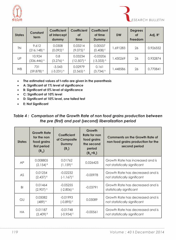
States Constant term
Coefficient of Intercept
dummy
Coefficient of
time
Coefficient of time Dummy
DWDegrees
of Freedom
Adj. R2
TN9.612
(216.148) A
0.0308(0.092) E
0.03214(9.075) E
0.00537 (0.408) E 1.691283 26 0.926552
UP10.924
(336.446) A
0.8(3.276) A
0.03234(12.507) A
-0.03206 (-3.333) A 1.430269 26 0.932874
WB731
(59.878) A
-3.543(-3.231) A
0.02979(2.565) A
0.161 (3.734) A 1.448586 26 0.770841
•► The estimated values of t-ratio are given in the parenthesis•► A: Significant at 1% level of significance•► B: Significant at 5% level of significance•► C: Significant at 10% level•► D: Significant at 10% level, one tailed test•► E: Not Significant
Table 4 : Comparison of the Growth Rate of non food grains production between the pre (first) and post (second) liberalization period
States
Growth Rate for the non food grains first period
(BO)
Coefficientof Composite
Dummy (B1)
Growth Rate for non food grains the second
period (BO+B1)
Comments on the Growth Rate of non food grains production for the
second period
AP0.008805 (2.154) B
0.01762 (1.159) E 0.026425
Growth Rate has increased and is not statistically significant
AS0.01254 (2.437) B
-0.02232 (-1.167) E -0.00978
Growth Rate has decreased and is not statistically significant
BI0.01464 (2.907) A
-0.05255 (-2.806) A -0.03791
Growth Rate has decreased and is statistically significant
GU0.05082 (489) A
-0.01993 (-0.895) E 0.03089
Growth Rate has decreased and is not statistically significant
HA0.01187 (2.409) B
-0.01748 (-0.954) E -0.00561
Growth Rate has decreased and is not statistically significant
ESEARCH BULLETIN
119 Volume : 40 I December 2014

States
Growth Rate for the non food grains first period
(BO)
Coefficientof Composite
Dummy (B1)
Growth Rate for non food grains the second
period (BO+B1)
Comments on the Growth Rate of non food grains production for the
second period
HP0.00514 (0.431) E
0.01482 (0.334) E 0.01996
Growth Rate has increased but is not statistically significant
JK0.00564 (0.766) E
0.0795 (2.904) A 0.08514
Growth Rate has increased and is statistically significant
KA0.03439
(12.605) A
0.04145 (4.085) A 0.07584
Growth Rate has increased and is statistically significant
KE-0.06958 (-7.654) A
0.199 (5.873) A 0.12942
Growth Rate has increased and is statistically significant
MH0.04361 (472) A
-0.02138 (-1.117) E 0.02223
Growth Rate has decreased and is not statistically significant
MP0.01762 (4.117) A
-0.005284 (-0.332) E 0.012336
Growth Rate has decreased and is not statistically significant
OR0.02331 (7.035) A
-0.121 (-9.853) A -0.09769
Growth Rate has decreased and is statistically significant
PU0.00808 (1.924) D
-0.02398 (-1.535) D -0.0159
Growth Rate has decreased and is not statistically significant
RA0.02004 (3.027) B
-0.05735 (-2.329) B -0.03731
Growth Rate has decreased and is statistically significant
TN0.03214 (9.075) E
0.00537 (0.408) E 0.03751
Growth Rate has increased and is not statistically significant
UP0.03234
(12.507) A
-0.03206 (-3.333) A 0.00028
Growth Rate has decreased and is statistically significant
WB0.02979 (2.565) A
0.161 (3.734) A 0.19079
Growth Rate has increased and is statistically significant
•► The estimated values of t-ratio are given in the parenthesis•► A: Significant at 1% level of significance•► B: Significant at 5% level of significance
ESEARCH BULLETIN
120Volume : 40 I December 2014

•► C: Significant at 10% level•► D: Significant at 10% level, one tailed test•► E: Not Significant
Table 5 : Estimation of dummy variable model to find out shift in growth path of total agricultural production for different states of India taking 1991-92 as the break point
States Constant term
Coefficient of
Intercept dummy
Coefficient of
time
Coefficient of time Dummy
DWDegrees
of Freedom
Adj. R2
AP9.955
(249.942)A
-0.194(-0.649) E
0.01477(4.658) A
0.01098(0.931) E 1.168396 26 0.780961
AS591
(217.116) A0.263
(0.885) E0.01618(5.134) A
-0.01294(-1.104) E
1.40838 26 0.619132
BI9.556
(293.121) A0.756
(3.085) A0.01762(6.788) A
-0.0306(-3.169) A
0.743082 26 0.786177
GU9.09
(119.634) A0.375
(0.657) E
0.03883(6.416) A
-0.01658(-0.737) E
1.133216 26 0.777249
HA9.222
(24428) A0.235
(0.843) E0.0281
(9.506) A-0.009152(-0.832) E
0.727206 26 0.897816
HP6.896
(173.528) A0.412
(1.378) D0.01681(5.31) A
-0.01329(-1.129) E
0.749851 26 0.788507
JK6.945
(223.517) A1.166
(4.992) A0.01789
(7.231) A-0.04766(-5.178) A
0.951567 26 0.793991
KA9.516
(163.338) A-0.702
(-1.602) D0.03863(326) A
0.03025(1.753) C
1.459034 26 0.896444
KE969
(103.709) A-3.1
(-4.767) A-0.05289(-7.68) A
0.145(5.642) A
0.546367 26 0.715596
MH10.053
(156.01) A0.596
(1.23) E0.03885(7.57) A
-0.02345(-1.229) E
0.55238 26 0.842897
MP9.439
(89.98) A1.283
(1.626) D0.02052
(2.457) A-0.04862(-1.565) D
2.160977 26 0.361688
OR995
(360.692) A1.877
(10.006) A0.02261
(11.384) B-0.0892
(-12.075) A1.656381 26 0.890681
PU9.544
(429.83) A0.503
(3.011) A0.03517
(19.888) A-0.02245(-3.413) A
1.091101 26 0.969401
ESEARCH BULLETIN
121 Volume : 40 I December 2014

States Constant term
Coefficient of
Intercept dummy
Coefficient of
time
Coefficient of time Dummy
DWDegrees
of Freedom
Adj. R2
RA9.013
(167.084) A0.649(1.6) D
0.02475(5.762) A
-0.02458(-1.538) D
1.031613 26 0.765435
TN9.985
(230.377) A-0.02549(-0.078) E
0.02472(7.161) A
0.008145(0.634) E
1.79951 26 0.9025
UP11.169
(486.41) A0.701
(4.062) A0.0352
(19.248) A-0.02978(-4.378) A
1.449712 26 0.967927
WB9.492
(91.93) A-2.343
(-3.018) A0.02524(3.069) A
0.109(3.558) A
1.461413 26 0.802083
The estimated values of t-ratio are given in the parenthesisA: Significant at 1% level of significanceB: Significant at 5% level of significanceC: Significant at 10% levelD: Significant at 10% level, one tailed testE: Not Significant
Table 6 : Comparison of the Growth Rate of total agricultural production between the pre (first) and post (second) liberalization period
States
Growth Rate for total agricultural production for the first period
(BO)
Coefficientof
Composite Dummy (B1)
Growth Rate for total agricultural production the second period
(BO+B1)
Comments on the Growth Rate of yield of total agricultural production for the second
period
AP0.01477(4.658) A
0.01098(0.931) E 0.02575
Growth Rate has increased but is not statistically significant
AS0.01618(5.134) A
-0.01294(-1.104) E 0.00324
Growth Rate has decreased and is not statistically significant
BI0.01762(6.788) A
-0.0306(-3.169) A -0.01298
Growth Rate has decreased and is statistically significant
GU0.03883(6.416) A
-0.01658(-0.737) E 0.02225
Growth Rate has decreased and is not statistically significant
ESEARCH BULLETIN
122Volume : 40 I December 2014

States
Growth Rate for total agricultural production for the first period
(BO)
Coefficientof
Composite Dummy (B1)
Growth Rate for total agricultural production the second period
(BO+B1)
Comments on the Growth Rate of yield of total agricultural production for the second
period
HA0.0281
(9.506) A
-0.009152(-0.832) E 0.018948
Growth Rate has decreased and is not statistically significant
HP0.01681(5.31) A
-0.01329(-1.129) E 0.00352
Growth Rate has decreased and is not statistically significant
JK0.01789(7.231) A
-0.04766(-5.178) A -0.02977
Growth Rate has decreased and is statistically significant
KA0.03863(326) A
0.03025(1.753) C 0.06888
Growth Rate has increased and is statistically significant
KE-0.05289(-7.68) A
0.145(5.642) A 0.09211
Growth Rate has increased and is statistically significant
MH0.03885(7.57) A
-0.02345(-1.229) E 0.0154
Growth Rate has decreased and is not statistically significant
MP0.02052(2.457) A
-0.04862(-1.565) D -0.0281
Growth Rate has decreased and is statistically significant
OR0.02261
(11.384) B
-0.0892(-12.075) A -0.06659
Growth Rate has decreased and is statistically significant
PU0.03517
(19.888) A
-0.02245(-3.413) A 0.01272
Growth Rate has increased and is statistically significant
RA0.02475(5.762) A
-0.02458(-1.538) D 0.00017
Growth Rate has decreased and is statistically significant
TN0.02472(7.161) A
0.008145(0.634) E 0.032865
Growth Rate has increased and is not statistically significant
UP0.0352
(19.248) A
-0.02978(-4.378) A 0.00542
Growth Rate has decreased and is statistically significant
WB0.02524(3.069) A
0.109(3.558) A 0.13424
Growth Rate has increased and is statistically significant
ESEARCH BULLETIN
123 Volume : 40 I December 2014

•► The estimated values of t-ratio are given in the parenthesis•► A: Significant at 1% level of significance•► B: Significant at 5% level of significance•► C: Significant at 10% level•► D: Significant at 10% level, one tailed test•► E: Not Significant
Table 7 : Estimation of dummy variable model to find out the shift in growth path of yield of food grains production for different states of India taking 1991-92 as the
break point
States Constant term
Coefficient of Intercept
dummy
Coefficient of time
Coefficient of
time Dummy
DWDegrees
of Freedom
Adj. R2
AP736
(7172)A
4.885(5.812) A
0.01983(2.228) B
-0.237(-7.146) A 1.290258938 26 0.833277016
AS7.77
(106.416)
A
1.502(2.735) A
0.03401(5.849) A
-0.109(-5.035) A 1.463278194 26 0.876839967
BI602
(71.035) A
5.818(6.388) A
0.03257(3.378) A
-0.284(-7.92) A 1.307785401 26 0.849643326
GU972
(70.342) A
4.144(4.32) A
0.008851(0.871) E
-0.22(-5.811) A 1.505542015 26 0.869789043
HA865
(73.608) A
5.29(5.84) A
0.03007(3.135) A
-0.251(-7.023) A 1.255836026 26 0.777255798
HP697
(69.232) A
4.657(4.928) A
0.003966(0.396) A
-0.215(-5.782) A 0.988317274 26 0.765964031
JK472
(99.908) A
4.194(6.576) A
0.01798(2.663) E
-0.206(-204) A 1.099330596 26 0.877597843
KA9.213
(7719) A
4.742(5.387) A
-0.006505(-0.698 ) B
-0.235(-6.785) A 1.154668371 26 0.897477087
KE7.242
(6407) A
4.277(5.372) A
0.05681(6.738) E
-0.199(-6.345) A 0.606155502 26 0.690747101
MH694
(61.024) A
6.559(6.121) A
0.01914(1.686) D
-0.32(-7.587) A 1.35931993 26 0.869831713
ESEARCH BULLETIN
124Volume : 40 I December 2014

States Constant term
Coefficient of Intercept
dummy
Coefficient of time
Coefficient of
time Dummy
DWDegrees
of Freedom
Adj. R2
MP699
(62.7) A
6.288(6.026) A
0.02026(1.834) C
-0.304(-7.409) A 1.215385839 26 0.853823807
OR722
(70.578 ) A
5.612(6.038) A
0.01893(1.924) C
-0.279(-7.626) A 1.154609852 26 0.87960214
PU9.12
(109.571)
A
3.618(5.781) A
0.02513(3.792) A
-0.185(-7.513) A 1.259013105 26 0.86258105
RA678
(55.41) A
6.548(5.559) A
0.01947(1.561) D
-0.315(-6.798) A 1.318011387 26 0.828812
TN737
(7422) A
4.603(5.493) A
0.02675(3.014) A
-0.228(-6.913) A 1.372730002 26 0.823785961
UP9.026
(65.061) A
5.409(5.184) A
0.02977(2.694) B
-0.271(-6.604) A 1.273108761 26 0.826446884
WB 858(91.448) A
3.696(5.074) A
0.01441(1.868) C
-0.187(-6.531) A 1.19172591 26 0.851420128
•► Estimated values of the‘t’ ratios are given in the parenthesis. •► A: Significant at 1% level of significance•► B: Significant at 5% level of significance•► C: Significant at 10% level•► D: Significant at 10% level, one tailed test•► E: Not Significant
Table 8 : Comparison of the growth rate of yield of food grains production between the pre (first) and post (second) liberalization period
States
Growth Rate of yield of food grains for the
first period (B2O)
Coefficientof
Composite Dummy
(B21)
Growth Rate of yield of food grains for the
second period (B2O+B21)
Comments on the Growth Rate yield of food grains production for
the second period
AP0.01983 (2.228) B
-0.237 (-7.146) A -0.21717
Growth rate of yield has decreased and is statistically significant
ESEARCH BULLETIN
125 Volume : 40 I December 2014

States
Growth Rate of yield of food grains for the
first period (B2O)
Coefficientof
Composite Dummy
(B21)
Growth Rate of yield of food grains for the
second period (B2O+B21)
Comments on the Growth Rate yield of food grains production for
the second period
AS0.03401 (5.849) A
-0.109 (-5.035) A -0.07499
Growth rate of yield has decreased and is statistically significant
BI0.03257 (3.378) A
-0.284 (-7.92) A -0.25143
Growth rate of yield has decreased and is statistically significant
GU0.008851 (0.871) E
-0.22 (-5.811)
A -0.21115Growth rate of yield has decreased and is statistically significant
HA0.03007 (3.135)
A
-0.251 (-7.023) A -0.22093
Growth rate of yield has decreased and is statistically significant
HP0.003966 (0.396) A
-0.215 (-5.782) A -0.21103
Growth rate of yield has decreased and is statistically significant
JK0.01798 (2.663)
E -0.206 (-204) A -0.18802Growth rate of yield has decreased and is statistically significant
KA-0.00650 (-0.698
) B
-0.235 (-6.785) A -0.24151
Growth rate of yield has decreased and is statistically significant
KE0.05681 (6.738)
E
-0.199 (-6.345) A -0.14219
Growth rate of yield has decreased and is statistically significant
MH0.01914 (1.686)
D
-0.32 (-7.587)
A -0.30086Growth rate of yield has decreased and is statistically significant
MP0.02026 (1.834)
C
-0.304 (-7.409) A -0.28374
Growth rate of yield has decreased and is statistically significant
OR0.01893 (1.924)
C
-0.279 (-7.626) A -0.26007
Growth rate of yield has decreased and is statistically significant
ESEARCH BULLETIN
126Volume : 40 I December 2014

States
Growth Rate of yield of food grains for the
first period (B2O)
Coefficientof
Composite Dummy
(B21)
Growth Rate of yield of food grains for the
second period (B2O+B21)
Comments on the Growth Rate yield of food grains production for
the second period
PU0.02513 (3.792)
A
-0.185 (-7.513) A -0.15987
Growth rate of yield has decreased and is statistically significant
RA0.01947 (1.561)
D
-0.315 (-6.798) A -0.29553
Growth rate of yield has decreased and is statistically significant
TN0.02675 (3.014)
A
-0.228 (-6.913) A -0.20125
Growth rate of yield has decreased and is statistically significant
UP0.02977 (2.694)
B
-0.271 (-6.604) A -0.24123
Growth rate of yield has decreased and is statistically significant
WB0.01441 (1.868)
C
-0.187 (-6.531) A -0.17259
Growth rate of yield has decreased and is statistically significant
•► The estimated values of t-ratio are given in the parenthesis•► A: Significant at 1% level of significance•► B: Significant at 5% level of significance•► C: Significant at 10% level•► D: Significant at 10% level, one tailed test•► E: Not Significant
Table 9 : Estimation of dummy variable model to find out the shift in growth path of yield of non food grains production for different states of India taking 1991-92 as
the break point
StatesConstant
term
Coefficient of Intercept
dummy
Coefficient of time
Coefficient of time Dummy
DWDegrees
of Freedom
Adj. R2
AP10.155
(111.452)A
0.881(1.285) E
0.07332(10.105) A
-0.05084(-1.884) C 0.474835076 26 0.852264251
AS10.023
(126.101) A
1.046(1.749) C
0.06354(10.038) A
-0.05883(-2.499) B 0.522953194 26 0.831123038
ESEARCH BULLETIN
127 Volume : 40 I December 2014

StatesConstant
term
Coefficient of Intercept
dummy
Coefficient of time
Coefficient of time Dummy
DWDegrees
of Freedom
Adj. R2
BI9.88
(142.505) A
1.41(2.704) B
0.06486(11.747) A
-0.06832(-3.327) A 0.374173255 26 0.889675857
GU10.792
(141.938) A
1.17(2.046) C
0.06953(11.482) A
-0.06517(-2.894) A 0.731519136 26 0.866865216
HA9.635
(7854) A
1.512(1.646) D
0.08228(455) A
-0.08093(-2.236) B 1.453850224 26 0.782165166
HP9.203
(146.66) A
-0.02215(-0.047) E
0.03522(7.048) A
0.02287(1.231) E 0.729337115 26 0.939985734
JK9.859
(169.251) A
0.666(1.519) D
0.01773(3.823) A
-0.01964(-1.138) E 0.875222142 26 0.731653676
KA9.975
(96.918) A
1.387(1.792) C
0.09191(11.213) A
-0.07268(-2.384) B 0.455865258 26 0.881957974
KE9.692
(7505) A
1.302(1.402) D
0.08985(9.139) A
-0.0687(-1.879) C 1.0827005 26 0.832358381
MH10.366
(124.27) A
1.132(1.804) C
0.07476(11.253) A
-0.06374(-2.58) B 0.527391656 26 0.867407443
MP10.178
(133.636) A
0.454(0.793) E
0.05342(808) A
-0.02788(-1.236) E 1.160442109 26 0.826875693
OR9.963
(90.96) A
1.51(1.833) C
0.08249(9.457) A
-0.08545(-2.634) B 0.479733566 26 0.800253629
PU9.745
(101.145) A
1.728(2.385) B
0.08541(11.131) A
-0.0911(-3.192) A 0.597892888 26 0.859852583
RA9.558
(95.813) A
2.157(2.875) A
0.08567(10.784) A
-0.104(-3.525) A 0.486674175 26 0.863613574
TN10.511
(10289) A
1.642(2.249) B
0.08223(10.638) A
-0.08277(-2.879) A 0.479686828 26 0.86244915
UP9.943
(142.109) A
1.485(2.821) A
0.08726(15.659) A
-0.07643(-3.688) A 0.503223043 26 0.934509438
WB9.967
(117.287) A
1.791(2.803) A
0.08463(12.506) A
-0.09047(-3.594) A 0.438825669 26 0.893415577
•► Estimated values of the‘t’ ratios are given in the parenthesis. •► A: Significant at 1% level of significance•► B: Significant at 5% level of significance•► C: Significant at 10% level•► D: Significant at 10% level, one tailed test•► E: Not Significant
ESEARCH BULLETIN
128Volume : 40 I December 2014

Table 10 : Comparison of the growth rate of yield of non food grains production between the pre (first) and post (second) liberalization period
States
Growth Rate of yield of non food grains for the first period
(B2O)
Coefficientof Composite Dummy (B21)
Growth Rate of yield of non food grains for
the second period
(B2O+B21)
Comments on the Growth Rate of yield of non food grains production for the
second period
AP0.07332
(10.105) A-0.05084(-1.884) C
0.02248
Growth Rate of yield of non food grains production has declined and is statistically significant
AS0.06354
(10.038) A-0.05883(-2.499) B
0.00471
Growth Rate of yield of non food grains production has declined and is statistically significant
BI0.06486
(11.747) A-0.06832(-3.327) A
-0.00346
Growth Rate of yield of non food grains production has declined and is statistically significant
GU0.06953
(11.482) A-0.06517(-2.894) A
0.00436
Growth Rate of yield of non food grains production has declined and is statistically significant
HA0.08228(455) A
-0.08093(-2.236) B
0.00135
Growth Rate of yield of non food grains production has declined and is statistically significant
HP0.03522(7.048) A
0.02287(1.231) E
0.05809
Growth Rate of yield of non food grains production has increased but not statistically significant
JK0.01773(3.823) A
-0.01964(-1.138) E
-0.00191
Growth Rate of yield of non food grains production has decreased but not statistically significant
ESEARCH BULLETIN
129 Volume : 40 I December 2014

States
Growth Rate of yield of non food grains for the first period
(B2O)
Coefficientof Composite Dummy (B21)
Growth Rate of yield of non food grains for
the second period
(B2O+B21)
Comments on the Growth Rate of yield of non food grains production for the
second period
KA0.09191
(11.213) A-0.07268(-2.384) B
0.01923
Growth Rate of yield of non food grains production has decreased and is statistically significant
KE0.08985(9.139) A
-0.0687(-1.879) C
0.02115
Growth Rate of yield of non food grains production has decreased and is statistically significant
MH0.07476
(11.253) A-0.06374(-2.58) B
0.01102
Growth Rate of yield of non food grains production has decreased and is statistically significant
MP0.05342(808) A
-0.02788(-1.236) E
0.02554
Growth Rate of yield of non food grains production has decreased but not statistically significant
OR0.08249(9.457) A
-0.08545(-2.634) B
-0.00296
Growth Rate of yield of non food grains production has decreased and is statistically significant
PU0.08541
(11.131) A-0.0911
(-3.192) A-0.00569
Growth Rate of yield of non food grains production has decreased and is statistically significant
RA0.08567
(10.784) A-0.104
(-3.525) A-0.01833
Growth Rate of yield of non food grains production has decreased and is statistically significant
ESEARCH BULLETIN
130Volume : 40 I December 2014

States
Growth Rate of yield of non food grains for the first period
(B2O)
Coefficientof Composite Dummy (B21)
Growth Rate of yield of non food grains for
the second period
(B2O+B21)
Comments on the Growth Rate of yield of non food grains production for the
second period
TN0.08223
(10.638) A-0.08277(-2.879) A
-0.00054
Growth Rate of yield of non food grains production has decreased and is statistically significant
UP0.08726
(15.659) A-0.07643(-3.688) A
0.01083
Growth Rate of yield of non food grains production has decreased and is statistically significant
WB0.08463
(12.506) A-0.09047(-3.594) A
-0.00584
Growth Rate of yield of non food grains production has decreased and is statistically significant
•► The estimated values of t-ratio are given in the parenthesis•► A: Significant at 1% level of significance•► B: Significant at 5% level of significance•► C: Significant at 10% level•► D: Significant at 10% level, one tailed test•► E: Not Significant
References
Dhar Arpita and Pal Dipyaman (2006): “Inter District disparity of food grains Produc-tion in West Bengal: Growth, Instability and Determinations of Yield,” Artha Beekashan, Vol. 14, No. 3 & 4, 293 – 312.
Ghose, Arpita and Pal Dipyaman (2007): “Growth of food grains Production: An Inter District Comparison of West Bengal”, Artha Beekashan, Vol. 15, No. 4 March 2007, 216 – 233.
Ray, S.C. (2004): Data Envelopment Analysis: Theory and Technique for Economics and Operation Research, Cambridge University Press
ESEARCH BULLETIN
131 Volume : 40 I December 2014


Introduction
Insurance sector is a major contributor to the financial savings of the household sector in the country, which can be channelized for various investment opportunity and purposes. Efforts at increasing consumer awareness and putting the regulatory framework for protection of pol-icyholder’s interest have been made both the industry and authoritarian level. Life insurance sector have ample growth possibilities. It is the only financial service which provides return in addition to the life risk exposures. The prospects for expansion and spread of life insurance in India is high due to large population and no pension system among larger work groups which lead to no old age income the insurance sector provides for the long term contractual savings for the investors. Life insurance can accumulate huge amounts of capital over time which can be invested productively in the economy.
Objectives
The main objectives of the paper are
►► To examine the status of Indian Life In-surance Industry at world market in terms of premium underwritten, market shares captured; and
►► To discover the ways to strengthen the per-formances of Indian life Insurance sector.
India’s Standing in Global Life Insurance Market : A Brief Analysis
Pooja ChoudharyAbstract
Life insurance is vital for a country’s risk management system, financial security and influences the growth of economy. The potential development of sector heavily depends on the efficiency of life insurers that how they are fulfilling the needs and expectations of customers. It helps to change the insights and opinion of the Indian people and to make them aware about insurable risks & benefits of insurance. There was a remarkable improvement in the life insurance industry in post insurance reform period which was featured by entry of private insurers in collaboration foreign giants. Due to this large number of unreached population facilitated with open reach to life insurance policies with limited restrictions. But still, life insurance coverage in Indian economy is quite untapped. Consequently, this paper attempts to examine the status of Indian Life Insurance Industry at world market in terms of premium underwritten, market shares captured.
Keywords
Steady Growth, Slow Market Saturation, Regulatory Controls, Innovative Product Portfolio.
ESEARCH BULLETIN
133 Volume : 40 I December 2014

Research Methodology
This paper is descriptive in nature stating facts about Indian life Insurance Industry at world level. For this study, a sample size of top 20 countries has been selected on the basis of ranking in world life insurance market during 2013-14. Data of 10 years from 2005 to 2014 have been taken into consideration. In order to measure the status of Indian life insurance sector at world level, premium income and market shares have been taken into consideration as determinants. World Annual reports from Swiss Re Sigma have been used to get required data. To statistical analysis of the data one way analysis of variances (One Way ANOVA) are used.
One Way ANOVA is used to find out the significant relation between more than two groups of variables. The process of ANOVA consists of deviations of two different variables of population variance from the data. Then the statistics is calculated from the ratio of two estimates. One is the measure of the effect of independent variables combined with error variance itself called as between group variance. The other estimate is the within group variances. In ANOVA, F ratio is the ratio of between and within group variances 1 .
A Brief Look on Life Insurance Industry in India
A. Life Insurance Industry in India in Pre- Insurance Sector Reforms
During pre insurance sector reform periods, Indian insurance industry was fully under the
control of government, as insurance companies were bound to work within India, not worldwide. Life Insurance came to India in the year 1818 from England. Oriental Life Insurance Company started in Calcutta was the first life insurance company in India. In 1829, the Madras Equitable had begun transacting life insurance business in the Madras Presidency. Indian Life Assurance Companies Act, 1912 was the first statutory measure to regulate life business. In 1928, the Indian Insurance Companies Act was passed to facilitate the Government to collect statistical information about life and non-life business transacted in India by Indian and foreign insurers including provident insurance societies. In 1938, with a view to protecting the interest of the Insurance public, the earlier legislation was consolidated and amended by the Insurance Act, 1938 with comprehensive provisions for effective control over the activities of insurers 2.
The demand for nationalisation of life insurance industry was made repeatedly in the past but it gathered momentum in January 19, 1956, when life insurance business in India was nationalised. In nationalisation 154 Indian insurance companies, 16 non-Indian companies and 75 provident societies were merged. The Parliament of India passed the Life Insurance Corporation Act on June 19, 1956, and the Life Insurance Corporation of India was created on 1st September, 1956.3 The Finance Minister C. D. Deshmukh at the time of piloting the bill for nationalisation states the objective of LIC- to conduct the business with utmost economy with the spirit of trusteeship; to charge premium no higher than warranted by strict actuarial considerations; to invest the
1 Gupta S. L. and Gupta Hitesh (2013): SPSS 17.0 for Researchers; International Book House Publication Limited, New Delhi, p. 94 2 History of insurance in India; Insurance Regulatory and Development Authority (IRDA), retrieved from https://www.irda.gov.in/ADMINCMS/cms/LayoutPages_Print.aspx?page=PageNo4 on September 16, 2014.3 Brief History of Insurance and Life Insurance; from the Website of Life Insurance Corporation of India, retrieved from https://www.licindia.in/history.htm on September 16, 2014.
ESEARCH BULLETIN
134Volume : 40 I December 2014

funds for obtaining maximum yield for the policy holders consistent with safety of capital; to render prompt and efficient service to policy holders thereby making insurance widely popular.4 In the pre globalisation era, there was monopoly of LIC in life insurance business in India.
B. Indian Life Insurance Industry in Post- Insurance Sector Reforms
In Indian life insurance the major changes occur in the form of Insurance Sector Reforms. Viewing competition in the market, The Indian Government appoints the Malhotra Committee in 1994 This committee was headed by former Finance Secretary and RBI Governor, R. N. Malhotra. The committee was aimed at creating a more efficient and competitive financial system suitable for the requirement of the economy keeping in mind the structural changes currently underway and recognising that insurance is an important part of overall financial system where it was necessary to address the need for similar reforms. In 1994 committee submit its report giving various recommendations in the form of structure, competition, investments and customer services related to insurance business in India. It was decided that competition allowed in a limited way by stipulating the minimum requirement of capital of Rs. 1 billion. The amount decided was not very high for private and foreign investors. Foreign equity participation was restricted to 40%.
Keeping in view the Malhotra Committee recommendations to set up independent regulatory body to regulate insurance business, IRDA bill was drafted, thus the government
ruled out the privatisation of public companies like LIC. It provides a regulatory body having 9 members with statutory powers. When the bill was introduced in parliament for first time, there were mix reactions about the problems, but in the year 1999, bill was finally passed and IRDA was established to promote, regulate, manage and control the insurance business in India as there was need arises because of moving the Indian insurance business to global market.
The opening of a new era of insurance progress has seen by the entry of global insurers, the explosion of pioneering products and distribution means and the increasing managerial standards.5 As on June 30, 2014, apart from Life Insurance Corporation the public sector life insurer, there are 23 other private sector life insurance companies operating in India, most of them joint ventures between Indian private companies and global insurance partners.
Global Life Insurance Market during 2013-14 : A Quick Look
The analysis and growth experience of the life insurance industry in the majority of countries shows that the intensifying and broadening of the life insurance services are positively connected to the extent of competition and the number of life insurers in the market. In a closed and controlled market situation, the growth of life insurance slows down. The countries which have followed the open and liberalised policy have informed quantum soar in the life insurance services.
Another trend is that the growth is higher in
4 Gupta P. K. (2011): Insurance and Risk Management; Himalaya Publishing House, Mumbai, 2011, p.189.5 Jain Yogesh (Jan. - Feb. 2013): Economic Reforms and World Economic Crisis: Changing Indian Life Insurance market place; IOSR Journal of Business and Management (IOSR-JBM), Volume 8, Issue 1 (Jan. - Feb. 2013), pp.106-115; retrieved from www.iosrjournals.org on September 14, 2014.
ESEARCH BULLETIN
135 Volume : 40 I December 2014

those countries where relatively less controls were enforced on life insurance industries.6 From the annual reports of Swiss Re, Sigma it has been seen that the total world life insurance premium volume decreased at USD 2608091 million during 2013 compared to 2012 which was USD 2630274 million. Meaning is that the total life insurance premium volume declined by 0.8 percent over previous year’s premium underwritten. Similarly the life insurance density of total world life insurance also reduced to USD 366.00 during 2013-14 compared to USD 372.6 in 2012-13. Penetration of total world life insurance reduced during 2013-14 to 3.5 percent of total GDP compared to life insurance penetration at 3.69 percent of total GDP during 2012-13.
India’s Position at Global Life Insurance Market: A Comparative Analysis
Taking the case of particular paper, among top 20 countries of world in global life insurance market during 2013-14, India ranked 11th as per data published by Swiss Re during 2013-14, the estimated life insurance premium in India decreased by 1.1% as compared to previous year. The market share of Indian life insurance sector in global market was 2.00 % during 2013-14 as against 2.03% in 2012-13. The insurance density of life insurance sector had downfall from USD 42.7 in 2013 to USD 41.00 in 2014. Similarly, insurance penetration had also declined from 3.17 percent in 2013 to 3.10 percent in 2013-14. For the analysis purpose, two determinants used i.e. life insurance premium volume in US Dollar and market shares captured in percent as a share of world life insurance market.
1. Life Insurance Premium Volume
Premium income is the major source of income of life insurance industry. Table 1 shows the total life
insurance premium underwritten by the different countries’ life insurance industry from 2004-05 to 2013-14. Accordingly mean value is found out and ranks given on the basis of corresponding mean value. table indicates that the premium volume of advanced market countries such as USA, China, Germany, Italy, South Korea, Japan etc. are quite high compared to developing market countries. Taking particular study of Indian life insurance industry, it has found that the income of industry declined slightly during 2013-14 compared to previous year’s performances.
It is observed from table 1 and its analysis through One Way ANOVA, viewing the Test of Homoge-neity of Variances table, the p-value of Levene’s statistic is less than 0.05 i.e. 0.000. It means the variances of group are not homogeneous and therefore differ significantly. In such a situation, result may not be valid for this variable. Thus, Brown-Forsythe and Welch test are performed for analysis purpose. Then analysis of the ANO-VA table, it has observed that the value of F with 19 and 180 degree of freedom is 285.367, results in a probability of 0.000. The critical value of F at 19 and 180 degree of freedom is 1.6446, which is very much low than the calculated val-ue. Again according to the rule of homogene-ity of variance, the variable will not be judged by F statistics in ANOVA. Using the Welch and Brown-Forsythe statistic, we find that F statistic (19, 66.097) is 9.037; p is 0.000 less than the sig-nificance level at 0.05. So it can be concluded that there is difference between the premium incomes underwritten by the life insurance indus-tries of different countries. Particularly, analysing the performance of Indian life insurance industry, it has observed that industry make a steady and continuous growth till 2011 but then it started de-clining which is not a good sign for economic growth.
6 Dash Swadesh Kumar and Pany Tushar Kanti (2013): Insurance Industry in India – Prospects and Challenges; Asian Journal of Multidimensional Research Vol.2 Issue 4, April 2013, pp. 48-51.
ESEARCH BULLETIN
136Volume : 40 I December 2014

Tabl
e 1:
Glo
bal L
ife In
sura
nce
Prem
ium
Und
erw
ritte
n (in
USD
mill
ions
)
Cou
ntrie
s20
04-
0520
05-
0620
06-
0720
07-
0820
08-
0920
09-
1020
10-
1120
11-
1220
12-
1320
13-
14M
ean
Valu
e
Rank
on
th
e ba
sis
of
Mea
n Va
lue
USA
5023
0251
7074
5336
4957
8357
5782
1149
2345
5062
2853
7570
5677
56
5328
5853
4635
.00
1Ja
pan
3898
4337
5958
3627
6633
0651
3671
1239
9100
4409
5052
4668
5243
72
4237
3341
3915
.30
2UK
19
3196
1996
1231
1691
3497
4034
2759
2176
8121
3831
2100
6720
5918
22
2893
2467
38.8
03
Fran
ce
1334
5615
4058
1779
0218
6993
1811
4619
4077
1924
2817
4753
1493
46
1601
5617
0431
.50
4PR
Chi
na
3444
939
552
4509
258
678
9583
110
9175
1429
9913
4539
1412
08
1521
2195
364.
407
Italy
82
083
9174
089
576
8821
582
623
1152
9012
2063
1050
8993
273
1179
7898
793.
006
Ger
man
y 84
697
9022
594
911
1024
1911
1278
1117
7511
4868
1138
6910
6411
11
4349
1044
80.2
05
Sout
h Ko
rea
4848
558
848
7229
881
298
6641
757
436
7113
179
161
7892
0 91
204
7051
9.80
8
Taiw
an
3327
938
808
4124
549
813
5274
852
202
6392
064
133
7252
2 75
013
5436
8.30
9C
anad
a29
013
3445
639
212
4559
347
855
4365
651
574
5216
751
783
5233
444
764.
3011
Ind
ia17
500
2017
537
220
4713
248
860
5711
467
810
6044
253
300
5217
446
172.
7010
Braz
il81
9910
556
1369
918
285
2241
924
781
3324
641
046
4478
4 49
417
2664
3.20
18Ire
land
19
068
2001
037
331
4993
334
055
3544
539
296
4303
842
625
4692
936
773.
0012
Aus
tralia
2571
927
602
2828
734
725
4269
732
468
3804
545
187
4368
9 45
641
3640
6.00
13So
uth
Afri
ca
2349
725
930
3310
634
927
3452
528
773
4318
641
534
4478
7 44
556
3548
2.10
14Sw
itzer
-la
nd
2431
322
747
2336
323
982
2712
226
379
2880
935
083
3377
1 34
227
2797
9.60
17
Spai
n 23
592
2551
828
285
3116
639
133
4218
634
676
3925
733
762
3386
233
143.
7015
Hong
Ko
ng
1263
615
340
1748
221
848
2132
420
269
2262
424
556
2897
9 32
059
2171
1.70
20
Swed
en
1886
615
850
2003
223
969
2590
324
904
2941
131
961
2727
5 30
865
2490
3.60
19N
ethe
r-la
nds
3106
131
914
3390
735
998
3889
933
758
2510
231
210
2933
8 26
005
3171
9.20
16
Sour
ce: C
ompi
led
and
com
pute
d fr
om W
orld
Insu
ranc
e Re
port
from
Sw
iss R
e, S
igm
a fro
m 2
005
to 2
014
ESEARCH BULLETIN
137 Volume : 40 I December 2014

Result and Interpretation
Test of Homogeneity of VariancesLife insurance premium volume in USD
Levene Statistic df1 df2 Sig.13.941 19 180 .000
ANOVALife insurance premium volume in USD
Sum of Squares
df Mean Square F Sig.
Between Groups 3.654E12 19 1.923E11 285.367 .000
Within Groups 1.213E11 180 6.738E8Total 3.775E12 199
Robust Tests of Equality of MeansPremium income
Statistica df1 df2 Sig.Welch 187.618 19 66.097 .000
285.367 19 40.634 .000a. Asymptotically F distributed.
Graph 1: Life Insurance Premium Volume in USD at World level
Life insurance Premium Volume
United StatesJapan
United KingdomFrance
PR ChinaItaly
GermanySouth Korea
TaiwanCanadaIndia
BrazilIrelandAustraliaSouth Africa
SwitzerlandSpain
Hong KongSweden
Netherlands
0 100000 200000 300000 400000 500000 600000
Coun
trie
s
Life Insurance Premium Volume in USD
ESEARCH BULLETIN
2. Life Insurance Market Shares
Market shares show the percent of life insurance market captured by each country’s life insurance industry. Table 2 presents the global life insurance market shares in terms of total premium earned by life insurance sector of different countries
selected for present study. Data has been taken from 2004-05 to 2013-14 from the annual reports of Swiss Re, Sigma. And on the basis of total values mean values are found out and ranks are given according to the mean value. Then for analysis purpose ANOVA is applied to find out
the required results as given below.
138Volume : 40 I December 2014

ESEARCH BULLETIN
139
Tabl
e 2:
Glo
bal L
ife In
sura
nce
Mar
ket S
hare
s (in
% o
f Tot
al P
rem
ium
Und
erw
ritte
n)
Cou
ntrie
s20
04-
0520
05-
0620
06-
0720
07-
0820
08-
0920
09-
1020
10-
1120
11-
1220
12-
1320
13-
14M
ean
Rank
on
the
Basis
of
M
ean
Valu
eUS
A26
.77
26.2
024
.15
24.1
723
.22
21.1
220
.09
20.4
621
.66
20.4
322
.827
01
Japa
n20
.93
19.0
516
.42
13.8
214
.74
17.1
217
.50
19.9
720
.01
16.2
117
.577
02
UK10
.26
10.1
114
.11
14.6
113
.76
9.34
8.49
8.00
7.86
8.
5510
.509
03
Fran
ce
6.97
7.81
8.05
7.81
7.27
8.32
7.64
6.65
5.70
6.
147.
2360
4PR
Chi
na
1.92
2.01
2.04
2.45
3.85
4.68
5.67
5.12
5.39
5.
833.
8960
7Ita
ly
4.44
4.65
4.05
3.69
3.32
4.94
4.84
4.00
3.56
4.
524.
2010
6G
erm
any
4.40
4.57
4.30
4.28
4.47
4.79
4.56
4.33
4.06
4.
384.
4140
5So
uth
Kore
a2.
632.
983.
273.
402.
672.
462.
823.
013.
01
3.50
2.97
508
Taiw
an
1.83
1.97
1.87
2.08
2.12
2.24
2.54
2.44
2.77
2.
882.
2740
9C
anad
a1.
601.
751.
771.
911.
921.
872.
051.
991.
98
2.01
1.88
5011
Ind
ia0.
921.
021.
681.
971.
962.
452.
692.
302.
03
2.00
1.90
2010
Braz
il0.
440.
530.
620.
760.
901.
061.
321.
561.
71
1.89
1.07
9018
Irela
nd
1.03
1.01
1.69
2.09
1.37
1.52
1.56
1.64
1.63
1.
801.
5340
12A
ustra
lia1.
391.
401.
281.
451.
711.
391.
511.
721.
67
1.75
1.52
7013
Sout
h A
frica
1.
321.
311.
501.
461.
391.
231.
711.
581.
71
1.71
1.49
2014
Switz
erla
nd
1.30
1.15
1.06
1.00
1.09
1.13
1.14
1.34
1.27
1.
311.
1790
17Sp
ain
1.28
1.29
1.28
1.30
1.57
1.68
1.38
1.49
1.29
1.
301.
3860
15Ho
ng K
ong
0.70
0.78
0.79
0.91
0.86
0.87
0.90
0.93
1.11
1.
23.9
080
20Sw
eden
0.
850.
960.
911.
001.
041.
071.
171.
221.
041.
181.
0440
19N
ethe
rland
s 1.
701.
621.
531.
501.
561.
451.
001.
191.
12
1.00
1.36
7016
Sour
ce: C
ompi
led
and
com
pute
d fr
om W
orld
Insu
ranc
e Re
port
of S
wiss
Re,
Sig
ma
from
200
5 to
201
4
Volume : 40 I December 2014

Result and Interpretation
Test of Homogeneity of VariancesLife insurance market shares at world level
Levene Statistic df1 df2 Sig.18.729 19 180 .000
ANOVALife insurance market shares at world level
Sum of Squares
df Mean Square F Sig.
Between Groups
6655.126 19 350.270 297.131 .000
Within Groups 212.191 180 1.179Total 6867.318 199
Robust Tests of Equality of MeansMarket Shares
Statistica df1 df2 Sig.Welch 187.618 19 66.097 .000
Brown-Forsythe 285.367 19 40.634 .000a. Asymptotically F distributed.
Graph 2 Life Insurance Market Shares at World Level
Life Insurance Market Shares at World Level
JapanUnited Kingdom
FrancePR China
ItalyGermany
South KoreaTaiwan
Canada
BrazilIrelandAustraliaSouth Africa
Spain
SwedenNetherlands
United States
India
Switzerland
Hong Kong
0 5 10 15 20 25
Coun
trie
s
Market Shares in Percentage
ESEARCH BULLETIN
It is examined from table 2 and its analysis, in the Test of Homogeneity of Variances table, the p-value of Levene's statistic is less than 0.05 i.e. 0.000. It means the variances of group differ significantly. Then analysis of the ANOVA table, it has observed that the value of F with 19 and 180 degree of freedom is 297.131, results in a proba1-
bility of 0.000. The critical value of F at 19 and 180 degree of freedom is 1.6446, which is very low than the calculated value. Again according to the rule of homogeneity of variance, the variable will not be judged by F statistics in ANOVA. Using the Welch and Brown-Forsythe statistic, we find that F statistic (19, 66.097) is 9.037; probability is 0.000
140Volume : 40 I December 2014

ESEARCH BULLETIN
141
less 0.05. So it can be concluded that there is dif-ference between the market shares retained by the life insurance industries of different countries. Specifically, examining the performance of India in life insurance industry, it has detected that the industry grows till 2010-2011 with capturing shares 2.69 percent of total world life insurance market. But then started failing during 2013-14 with 2.00 percent shares of total market, which is not a fine signal for industry’s as well country’s financial growth.
Impact of Global Economic Crisis of Indian Life Insurance Market
The world economy faces the most terrible economic crisis in the year 2008. The global economic crisis that started from mortgage home loan left no industry untouched by its effects. Banks, insurance industry, manufacturing industry every industry was affected by the financial crisis directly or indirectly. Global economic crisis was the greatest financial challenges to the world economy which was originated in USA. The global crisis has affected the Indian economy through financial markets, trade flows, and exchange rates. The economy has shown substantial flexibility to the global economic crisis by maintaining one of the highest growth rates in the world economy. Indian financial sector considered safe, sound and not expected to have a large impact of the great economic crisis. The services sector including banking and insurance sectors accounted for around 88% of the growth rate in real gross domestic product. The global economic crisis is a result of deep economic depression generally refers to business cycle contraction over an extended period of
time. It is a position when economic indicators like gross domestic product, employment, household incomes and profit go down and bankruptcies rates are go up. The financial crisis may be a banking crisis and the solvency of the insurance sector as a whole does not appear to be endangered. India has one of the largest insurance markets in the world. 7
“According to the IMF, banks have suffered higher credit losses than the insurers. The impact of this financial crisis on the global life insurance industry was mixed. American International Group (AIG) and FORTIS, offers not only insurance but also banking services. Majority of the losses made by AIG and Fortis were considerably from financial products other than insurance such as derivatives and banking activities. Though the impacts of the crisis in the financial market was limited due to the widespread diversification of investments by the insurers, India cannot afford to remain insulated from this due to the exposure of the financial institutions in the global financial market. AIG’s financial crisis has some substantial bluster on businesses in Indian market as AIG has a joint venture in life insurance sector with the Tata Group. On the other hand Fortis has a joint venture with IDBI Bank in India. The collapse of these life insurance players have harsh social penalty due to the fact that millions of middle and lower middle class people in India buy the life insurance products not just to take-care of themselves but the benefits for their family mem-bers. As a result, the social costs of such failure have more economic cost and the end sufferers will be the common policy holders”8 . That time assurance was given by IRDA to policyholders their money is safe after AIG get the access
7 Ashraf S. H. and Sharma Dhanraj (2011): Global Financial Crisis and Its Impact on Indian Insurance Industry; International Journal of Research in Commerce, Economics and Management, volume no. 1, no. 4, August 2011.8 Ghosh Amlan: Impact of Global Financial Crisis in the Life Insurance Sector in India; retrieved form http://papers.ssrn.com/sol3/papers.cfm?abstract_id=1639122 on December 12, 2014
Volume : 40 I December 2014

of Federal Reserve’s borrowing pane. In India, domestic insurance companies do not have any disclosure overseas due to the controlled invest-ment regulations of IRDA, which restricts insurers from investing funds abroad.
Reasons for Slow Saturation of Life Insurance Market in India
From the result is very much clear that Indian life insurance sector is neither in very comfortable position nor in worst position. For life insurance companies operating in Indian economy, it is not very easy and automatic process to capture the market or to increase the demand for life insurance policies. There are always some rea-sons exists for success and failure of any business, industry or corporate body. Life insurance sector is not exception to it, and consist of some hurdles in the slow saturation of market and growth of sector at global level. The world 2008 financial crisis and European debt crisis in 2011 has much affected the insurance sector in the country. The crash of this financial crisis on Indian life insur-ance sector is also affected significantly, as this sector is not disconnected with the global mac-roeconomic behaviours. Because of instability in financial market Unit Link Plans have not been capable to give adequate profits even after pe-riod of five years. There has been pouring in the give up of Unit Link Plans with policyholders sad with their returns even after the confine period of payment.
Similarly the levels of insurance literacy are very stumpy in Indian case, as a result people do not realise what life insurance is, what actually it cov-ers etc. Therefore life insurance is given smallest priority in the financial saving and safety of the people not only in illiterates even among the
literate people. Same applies in case of agents also. 9 In current market scenario India continues to be a developing nation and large segments of the population do not have sufficient money to make their needs to meet, thus life insurance remains as their last concern. Along with these prompt reasons some of the issues for slow market growth involve lack of effective communication and promotion measures, low awareness of life insurance in rural areas, improper distribution modes and organisational conflicts etc.
Suggestions to Improve the Position of Indian Life Insurance Industry at Global Level
I. Increasing the literacy levels is one way of curbing the slow market penetration. If the agents are proficiently qualified, they can sell large number of policies on need based to the customers. The qualified and knowledgeable persons can only provide the answers on need based as per the customer’s own budget, because the customers must know the exact reason for buying the insurance policy.
II. Most of the people in Indian economy, lives in rural areas or semi-urban areas and they do not have awareness or can say do not have any idea to access life insurance market or about life insurance policies. So it is very much essential for companies to tap the rural segment.
III. There should be a proper control and regulatory mechanism that may prevent the conflicts in the organisation among employees and officials for their personal interest and ben-efits.
IV. For better market capture, life insurers should develop such dynamic and unique pro-
ESEARCH BULLETIN
142
9 Ganesh S.S.S.Durga (2014): Growth of Insurance Industry In India After Privatization - Life Insurance Sector Is At An Inflection Point; Researchjournali’s Journal of Commerce, Vol. 2, No. 2, March 2014, retrieved from http://www.researchjournali.com/pdf/402.pdf on September, 23 2014.
Volume : 40 I December 2014

ESEARCH BULLETIN
143
motional campaign, so that all types of earning people can understand the benefits of investing money for financial security for personal and family’s well beings.
V. In India most of the population belongs to the lower-middle income groups. Thus, one of the main criteria for capturing Indian market is to develop innovative and price conscious policies to attract lower and middle income segment of market.
These are the few suggestions that can be useful for life insurance companies operating in Indian environment that can be useful at organisation-al/managerial level to curb relative hurdles in the way of successful implementation of busi-ness transactions as well as to improve market standings at global level.
Concluding Remarks
The observed results indicate that there is differ-ence between the countries in regards to life insurance premium underwritten and market shares captured accordingly. Particularly based on the analysis of study it can be said that the status of Indian life insurance sector is neither very satisfying nor very unsatisfactory. Because comparing to USA, China, Germany, South Korea, Japan, France, Italy, United Kingdom the premium income underwritten and market shares compared total business of India is quite low, while comparing to other nations like Brazil, Switzerland, Australia, South Africa, Spin, Hong-Kong, Netherlands the India’s status is very much acceptable and satisfactory. There are always some reasons exists for success and failure of any business, industry or corpo-rate body. The world 2008 financial crisis and European debt crisis in 2011 has much affected the insurance sector in the country. The crash of this financial crisis on Indian life insurance sector is also affected significantly, as this sector is not disconnected with the global macroeconomic
behaviours. There are some other reasons that hamper the fast market growth i.e. the lack of effective communication and promotion measures, low awareness of life insurance in rural areas, improper distribution modes and organ-isational conflicts, world financial crisis, uneven macroeconomic trends etc. these hurdles can be curb by taking initiatives to move industry to growth path through prevention of conflicts through regulatory measures, effective and attractive promotion strategy, increasing insur-ance literacy, tapping rural market and through to developing innovative and price conscious policies to attract lower and middle income people in India.
References
Article- Indian Insurance Sector Innovate Now or Stagnate; from Deloitte, retrieved from http://www.deloitte.com on August 29, 2014
Evolution of Life Insurance Industry in India; retrieved from http://www.dnb.co.in on September 12, 2014.
Ganesh S.S.S.Durga (2014): Growth of Insurance Industry In India After Privatization - Life Insurance Sector Is At An Inflection Point; Researchjournali’s Journal of Commerce, Vol. 2, No. 2, March 2014, retrieved from http://www.re-searchjournali.com/pdf/402.pdf on September, 23 2014.
Hymavathi Kumari (2013): Performance Evaluation of Indian Life Insurance Industry in Post Liberalization; International Journal of Social Sciences Arts and Humanities, Vol.1., No. 1, 2013; retrieved from http://crdeep.com, pp. 7-14.
Krishnamurthy Rajagopalan (2011): Life Insurance in India- Strategic Shifts in a Dynamic Industry; retrieved from https://www.towerswat-son.com/~/media/Pdf/.../1101-India-FIN.pdf on
Volume : 40 I December 2014

September 23, 2014.
Kaur Satvinder (2013): Unit – VI Life Insur-ance; retrieved from http://www.studymode.com on September 12, 2014
Life Insurance Marketing in India: The Changing Distribution Norms. Retrieved from www.icmrindia.org on September 13, 2014.
Lunawat M. L.: Insurance in India- Chang-ing Policies and Emerging Practices; Response Books, New Delhi.
Mathew M. J.: Insurance- Theory and Practices, RBSA Publishers, Jaipur, 1998.
Nirmal Ghorawat (2013): Perspective on Life Insurance Industry in India, retrieved from http://canirmalg.wordpress.com on September 13, 2014.
Report on Global view of the life in-surance market-How it is being shaped by the lingering; retrieved from About Ernst & Young; re-trieved from http://www.ey.com on September 29, 2014.
Srivastava Arnika, Tripathi Sarika and Kumar Amit (2012): Life Insurance Industry- The Challenging Trends; retrieved from http://www.researchersworld.com on September 29, 2014
Thakur Shilpa: Competition in Life Insurance Sector of India; retrieved from http://cci.gov.in
World Insurance Reports Swiss Re, Sigma from 2003-04 to 2012-13.
ESEARCH BULLETIN
144Volume : 40 I December 2014

IntroductionInflation has been a global phenomenon. Every nation has been facing it. There is only a difference in terms of degree i.e. one digit, two digit or three digit inflation. Emerging economies especially BRICS nations have also been facing inflation especially food inflation .Brazil, Russia, India, China and South Africa have been facing inflation that has affected the purchasing power of common or middle income people in a big way. Table 1 and Table 2 will highlight the overall trend of inflation in BRICS nations while analyzing its probable impact on purchasing power of the people.
Inflation Trends in BRICS Nations
Badar Alam IqbalLuciana Aparecida Bastos
Nayyar Rahman
Abstract
One of the biggest and more persisting issues at global level has been inflation. Brazil, Russia, India, China and South Africa are no exception to this notion. Keeping in mind, the significance, impact and consequences of inflation on general masses in Brazil, Russia, India, China and South Africa; the present paper tries to discuss the emerging trends and issues arising out of the inflation. The paper further suggests a strategy for minimizing the impact of inflation on common man’s purchasing power.
Keywords
Inflation, Consumer Price Index, BRICS
Table 1 : Annual Inflation (Average Consumer Prices)
Country Subject Descriptor Units 2008 2009 2010 2011 2012
BrazilInflation, average consumer prices
Percent change
5.678 4.888 5.039 6.636 5.404
ChinaInflation, average consumer prices
Percent change
5.900 -0.683 3.325 5.417 2.650
IndiaInflation, average consumer prices
Percent change
8.879 13.048 10.532 9.553 10.209
RussiaInflation, average consumer prices
Percent change
14.108 11.654 6.854 8.443 5.068
South Africa
Inflation, average consumer prices
Percent change
11.536 7.125 4.271 5.000 5.654
Source: International Monetary Fund, World Economic Outlook Database, April 2014, http://www.imf.org
ESEARCH BULLETIN
145 Volume : 40 I December 2014

Table 1 presents data for cross-comparison between BRICS nations. In 2008 Russia had the highest inflation rate and Brazil the lowest while in the subsequent year, that is, in 2009 India had highest inflation rate while China had a deflation instead of inflation. In 2010and 2011, India has remained the country with highest inflation rate while China witnessed lowest inflation rate. In the year 2012, the trend continued and India had the highest inflation rate and China the lowest in-flation rate. South Africa has shown a consistent fall in its inflation rate starting from 11.5% in 2008
to around 5% in 2011 and a little rise of additional 0.6% in 2012. It is to be noted that the data in Table 1 gives the average annual inflation that shows the impact on purchasing power of the people on an average rather than on time end basis. An analysis of Table 1 makes it crystal clear that the residents of Russia and India have lost their purchasing power to a greater extent in comparison to Brazil, South Africa and China. China has least eroded the purchasing power of the people. Chart 1 below shows the inflation trend in BRICS nations.
Chart 1
Source: Self-Prepared on the basis of data provided in Table 1
ESEARCH BULLETIN
It would also be interesting to note the inflation rate based on consumer prices but calculated at the year-end so as to understand inflation trend from another angle. Table 2 highlights the data with the same objective.
Table 2 : Rate of Inflation (End of Consumer Prices)
Country Subject Descriptor Units 2008 2009 2010 2011 2012
BrazilInflation, end of period consumer prices
Percent change
5.902 4.312 5.909 6.503 5.839
ChinaInflation, end of period consumer prices
Percent change
1.200 1.900 4.600 4.100 2.500
146Volume : 40 I December 2014

Country Subject Descriptor Units 2008 2009 2010 2011 2012
IndiaInflation, end of period consumer prices
Percent change
9.091 14.286 10.000 9.375 10.390
RussiaInflation, end of period consumer prices
Percent change
13.300 8.810 8.780 6.100 6.570
South Africa
Inflation, end of period consumer prices
Percent change
10.066 6.289 3.480 6.054 5.708
Source: International Monetary Fund, World Economic Outlook Database, April 2014http://www.imf.org
Table 2 highlights the rate of inflation at the year end. It is different from table 1 on the basis that the rate of inflation in table 1 is calculated on year-on-year basis. On the other hand the data given in table 2 is calculated at the end of the year. Thus, the data of table 2 relates to the actual inflation at the end of a year. With this background, in 2008 the country with highest inflation was Russia and with lowest was China. In 2009, India had highest inflation in terms of consumer price index and again China had lowest inflation rate. In 2010, 2011 and 2012 India had highest inflation with the figures of 10, 9.375
and 10.39, respectively. In same years (2010, 2011 and 2012), China had the lowest inflation with the figures of 4.6, 4.1 and 2.5 percent, re-spectively with the exception of year 2010 when South Africa had the lowest rate of inflation. This shows the vulnerability of Russia and India with respect to erosion of purchasing power due to high rate of inflation. Brazil encounters the same problem of high inflation but not to the extent of Russia. China and South Africa on the other hand has taken a leap in controlling inflation in the BRICS nations. Chart 2 shows the trends of year end inflation rate for BRICS nations.
ESEARCH BULLETIN
147
Chart 2
Source: Self-Prepared on the basis of data provided in Table 2
Volume : 40 I December 2014

Review of Literature
A review of past studies shows that inflation trends were specifically discussed under emerg-ing economies title. These studies focused on countries that also included BRICS nations. With respect to China, it was identified that inflation rate in China had been moderate over the past decades (Lin and Wang, 2013). In the same study conducted by Lin and Wang(2013) issue of inflation was given paramount importance not just due to monetary policy impact, con-sumption and investment but due to its spillover effects in the global economy. It was concluded that high inflation is not only threat to China but also to highly trade dependent countries such as South Korea. In most of the studies inflation targeting was accepted as a measure to control inflation (Samarina, Terpstra and De Haan, 2014). The pros and cons of inflation targeting has been exclusively discussed by various authors (e.g., Roger, 2009; Walsh, 2009; De Carvalho Filho, 2010). Goncalves and Salles (2008) and de Mendona and de Souza (2012) has identified that inflation targeting as a policy measure of central bank reduces and control inflation rates in emerging and developing economies. Thus, the conclusion of Salles & Souza applies to BRICS nations. However, it was identified by Samarina and De Haan (2013) that the factors leading to adoption of inflation targeting adoption differ significantly between OECD and non-OECD countries.
Past studies have identified two primary causes of inflation in China i.e. reform inflation and ex-cess demand inflation. Other BRICS nations also witness the same tendency (Yunqi, 1989). A cen-trally planned economy like China and Russia witness high inflation due to excess demand and to control it orders state enterprises to reduce investment spending and control consumption. In a market economy like Brazil, South Africa and India, the central bank use monetary policy to influence business spending by adjusting the
cost and availability of finance.
With respect to South Africa it has been identified that double digit inflation rate has been a major concern but success was achieved in 1990’s through an informal inflation targeting regime as it lowered the inflation rates (Amusa, Gupta, Karolia & Simo-Kengne, 2013).Formally, South African Reserve Bank used inflation targeting framework in Feb 2000 within a target of 3-6% (Mboweni, 2003; van der Merwe, 2004). Arestis, Ferrari-Filho and De Paula (2011), clearly stated that Brazil adhere religiously to the theoretical principles of the inflation targeting framework. Brazil has witnessed low economic growth with relatively high inflation. It was also identified that the macroeconomic literature has not conduct-ed a great deal of research on this important topic because of data limitations (Mazumder, 2014). After the currency crises of 1990s in Brazil, it adopted inflation targeting as a measure to con-trol rising inflation. During 1994-1998 the Brazilian government used high domestic interest rates with the objective of reducing inflation. Inflation targeting managed to reduce inflation in Brazil after its 1999and 2002 currency crises (Barbo-sa-Filho, 2008). Several authors have argued that for transition economies undergoing financial liberalization and integration in world financial markets inflation targeting is an attractive mone-tary policy framework (Jha, 2008).
Inflation Trends In Brazil
Brazil has faced a long inflationary period of 21 years from 1974 to 1994. During the 1980s and early 90s, Brazil witnessed the most critical period where inflation grew alarmingly. In order to look into the serious issue seven different stabilization plans were originated to contain rising prices, namely: The Cruzado Plan I , The Cruzado Plan II, The Bresser Plan, Policy Beans with Rice and Sum-mer-Plan in the Government of President José Sarney, Collor I and Collor II Plan under President Fernando Collor de Mello.Table 3 presents the
ESEARCH BULLETIN
148Volume : 40 I December 2014

figures for annual inflation in terms of average consumer prices with base of 100 and expressed as percent change. It shows that beginning from 1993, Brazil witnessed high inflation rates but later on due to the several plans initiated to curtail inflation, the consumer price index came down to a single figure in recent years ending to 2012. This shows that policies adopted by the country have attained the objective of curtailing inflation to single digits.
Table 3 : Annual Inflation (Average Consumer Prices Index)
YearCPI (Average Consumer
Price Index) percent change
1993 1,927.381994 2,075.831995 66.0081996 15.7571997 6.9261998 3.1961999 4.8592000 7.044
YearCPI (Average Consumer
Price Index) percent change
2001 6.842002 8.452003 14.7142004 6.5982005 6.872006 4.1842007 3.6412008 5.6782009 4.8882010 5.0392011 6.6362012 5.404
Source: International Monetary Fund, World Economic Outlook Database, April 2014
http://www.imf.org
On the other hand, Chart 3 shows the trend of in-flation in Brazil for the period starting from 1993 till 2012. It clearly shows that inflation was in double digit during early 1990s but eventually reached to single figure in 2012.
ESEARCH BULLETIN
149
Chart 3
Source: Self-Prepared on the basis of data provided in Table 3
Volume : 40 I December 2014

The table below shows the variation of the CPIE (Consumer Price Index Expanded) during the 1980s and early 90s. This index is used by Brazil to correct the balance sheets and quarterly finan-cial statements of public companies and is also the main index (official rate) used by the Central Bank of Brazil to measure inflation in the country.
Table 4 : Annual Variation of CPIE: 1980-1993
Year Consumer Price Index Expanded (%)
1980 99.271981 95.651982 104.801983 163.991984 215.271985 242.241986 79.651987 363.411988 980.221989 1972.911990 1620.961991 472.691992 1119.091993 2477.15
Source: Brazilian Institute of Geography and Statistics http://www.ibge.gov.br
Data expressed in Table 4 shows the evolution of inflation in the country, which peaked in 1993, when the CPIE stood at 2477.15%, demonstrating complete failure of all stabilization plans adopt-ed so far, as well as defeat of Brazilian monetary policy to stabilize prices.
However, from the government of President Fernando Henrique Cardoso (1994), with the creation, implementation and success of the Real Plan, Brazil began to live a moment of economic success with price stability, exchange
rate stability, drastic reduction of debt, external input of large volumes of foreign capital in the country and economic growth.With regard to price stability, Table 5 makes clear the change that occurred in Brazil after the Real Plan.
Table 5 : Annual variation of the CPIE: 1995-2011
Year Consumer Price Index Expanded (%)
1995 22.411996 9.561997 5.221998 1.661999 8.942000 5.972001 7.672002 12.532003 9.302004 7.602005 5.692006 3.142007 4.452008 5.902009 4.312010 5.902011 4.42
Source: Brazilian Institute of Geography and Statistics http://www.ibge.gov.br
Observe the drastic reduction of CPIE after the Real Plan, introduced in 1994. Although the 1990s were marked by financial crises in the international arena, namely the Mexican crisis in 1994, the Asian crisis in 1997 and the Russian crisis in 1998, the consequences of these crises did not pass dramatically in Brazil, to the point of compromising economic stability and economic growth on the rise.
ESEARCH BULLETIN
150Volume : 40 I December 2014
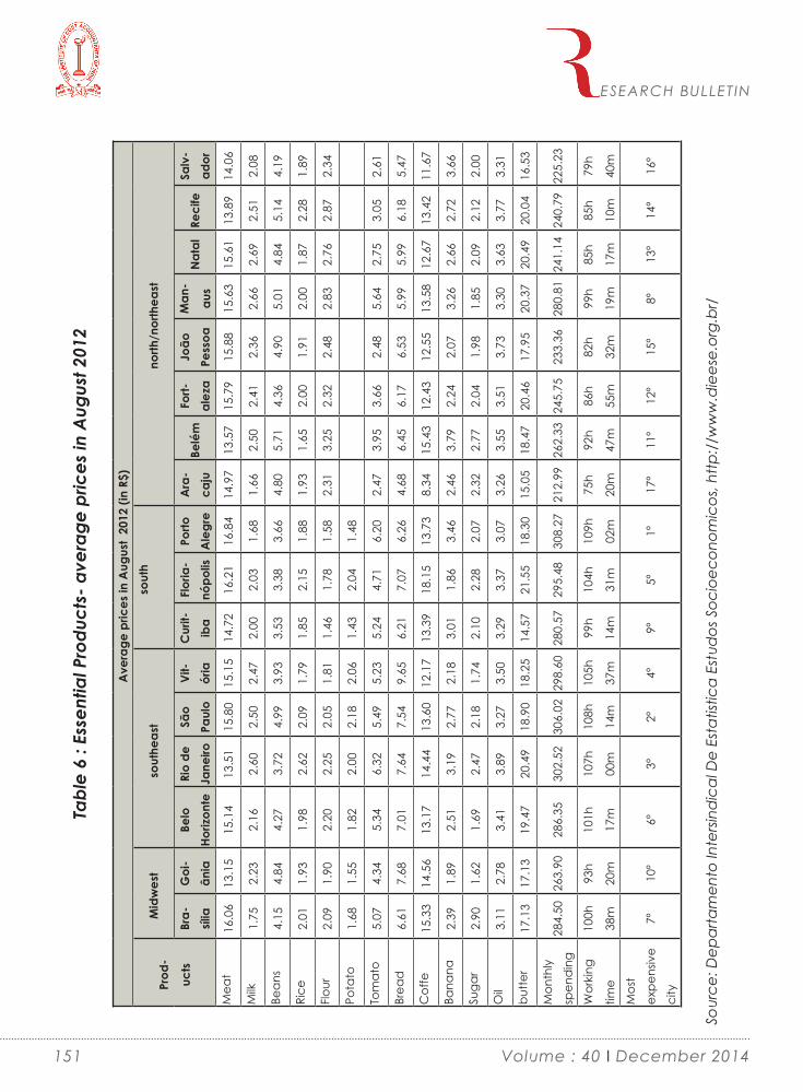
ESEARCH BULLETIN
151
Tabl
e 6
: Ess
entia
l Pro
duct
s- a
vera
ge p
rices
in A
ugus
t 201
2
Ave
rage
pric
es in
Aug
ust
2012
(in
R$)
Prod
-
ucts
Mid
wes
tso
uthe
ast
sout
h no
rth/n
orth
east
Bra-
sília
Goi
-ân
iaBe
lo
Horiz
onte
Rio
de
Jane
iroSã
o Pa
ulo
Vit-
ória
Cur
it-ib
aFl
oria
- nó
polis
Porto
A
legr
eA
ra-
caju
Belé
mFo
rt-al
eza
João
Pe
ssoa
Man
-
aus
Nat
alRe
cife
Salv
-ad
or
Mea
t16
.06
13.1
515
.14
13.5
115
.80
15.1
514
.72
16.2
116
.84
14.9
713
.57
15.7
915
.88
15.6
315
.61
13.8
914
.06
Milk
1.75
2.23
2.16
2.60
2.50
2.47
2.00
2.03
1.68
1.66
2.50
2.41
2.36
2.66
2.69
2.51
2.08
Bean
s4.
154.
844.
273.
724.
993.
933.
533.
383.
664.
805.
714.
364.
905.
014.
845.
144.
19
Rice
2.01
1.93
1.98
2.62
2.09
1.79
1.85
2.15
1.88
1.93
1.65
2.00
1.91
2.00
1.87
2.28
1.89
Flou
r2.
091.
902.
202.
252.
051.
811.
461.
781.
582.
313.
252.
322.
482.
832.
762.
872.
34
Pota
to1.
681.
551.
822.
002.
182.
061.
432.
041.
48
Tom
ato
5.07
4.34
5.34
6.32
5.49
5.23
5.24
4.71
6.20
2.47
3.95
3.66
2.48
5.64
2.75
3.05
2.61
Brea
d6.
617.
687.
017.
647.
549.
656.
217.
076.
264.
686.
456.
176.
535.
995.
996.
185.
47
Cof
fe15
.33
14.5
613
.17
14.4
413
.60
12.1
713
.39
18.1
513
.73
8.34
15.4
312
.43
12.5
513
.58
12.6
713
.42
11.6
7
Bana
na2.
391.
892.
513.
192.
772.
183.
011.
863.
462.
463.
792.
242.
073.
262.
662.
723.
66
Suga
r2.
901.
621.
692.
472.
181.
742.
102.
282.
072.
322.
772.
041.
981.
852.
092.
122.
00
Oil
3.11
2.78
3.41
3.89
3.27
3.50
3.29
3.37
3.07
3.26
3.55
3.51
3.73
3.30
3.63
3.77
3.31
butte
r17
.13
17.1
319
.47
20.4
918
.90
18.2
514
.57
21.5
518
.30
15.0
518
.47
20.4
617
.95
20.3
720
.49
20.0
416
.53
Mon
thly
spen
din
g28
4.50
263.
9028
6.35
302.
5230
6.02
298.
6028
0.57
295.
4830
8.27
212.
9926
2.33
245.
7523
3.36
280.
8124
1.14
240.
7922
5.23
Wor
king
time
100h
38m
93h
20m
101h
17m
107h
00m
108h
14m
105h
37m
99h
14m
104h
31m
109h
02m
75h
20m
92h
47m
86h
55m
82h
32m
99h
19m
85h
17m
85h
10m
79h
40m
Mos
t
expe
nsiv
e
city
7º10
º6º
3º2º
4º9º
5º1º
17º
11º
12º
15º
8º13
º14
º16
º
Sour
ce: D
epar
tam
ento
Inte
rsin
dic
al D
e Es
tatis
tica
Estu
dos
Soc
ioec
onom
icos
, http
://w
ww
.die
ese.
org.
br/
Volume : 40 I December 2014

Food Inflationin Brazil : 2012
Table 6 shows the essential products for the for the Brazilian consumer, their monthly spending with the purchase of these products and the necessary labor time so that they can be bought and the most expensive cities tofeed. The tables are divided by region and include the prices of essential food for consumption in the major capitals of the country.
Tables 6 show a list of 13 essential products that make up the basic food basket in Brazil by region, with emphasis onthe average prices of these products in August 2012. In addition, the table shows the work hours to buy these foods, as well as the ranking of themost expensive citiesto feed. Note thatin August 2012, the most expensive city for the Brazilian feed, with respect to products essential basic food basket was Porto Alegre, in the southern region, followed by SãoPaulo and Rio de Janeiroin the Region south east. The cheapest cities to feed during this period were Salvador, Recife and João Pessoa, respectively, all located in the North/Northeast. In August 2012, a worker residing in Porto Alegre, the most expensive city to feed in the period lacked 109 h 2 min work to acquire the products listed in the table. In relation to São Paulo, observe that in August 2012, people need to work 108 h 14 min to acquire the basic food basket, while in August 2013, has to work 103 h 43 min. Although São Pauloin 2013 has become the most expensive city to feed on the products of the basic basket of essential food of Brazilians, it is observed that food inflation has declined, as the number of hours that you have to work for the Brazilian buys these products in August 2012, declined in August 2013.
Reelection of President Dilma and Brazilian Economy : President Dilma Rousseff’s narrow victory has created two biggest challenges namely- restoration of confidence in Brazilian sluggish economy and poor services. The other
major challenge is to control inflation and keep check in deficit in budget. There is a need to design economic policy to meet the challenges. The changeover of the present Finance Minister may help in facing the challenges especially inflation and budget deficit. The coming years will show how far the new economic policy could help in checking the existing rate of inflation which is a persisting problem has to be tackled so that middle class could get relief which has given a second term to president Dilma Rousseff. The year 2015 would be the most crucial year for the Brazilian economy wherein the trends in regard to inflation may be available and may give insight to the challenge.
Inflation Trends In Russia
Russia has witnessed the highest inflation rates in the BRIC nations due to domestic as well as reasons related to its international trade. The monetary policy is to be blamed on one hand and inappropriate measures on the other hand. Table 7 presents the consumer price index from 1993 to 2012 to diagnose the issue.
Table 7 : Annual Inflation (Average Consumer Prices Index)
YearCPI (Average Consumer
Price Index) percent change
1993 874.6221994 307.6341995 197.4711996 47.7421997 14.7671998 27.6751999 85.7422000 20.7762001 21.4612002 15.7832003 13.666
ESEARCH BULLETIN
152Volume : 40 I December 2014

ESEARCH BULLETIN
153
YearCPI (Average Consumer
Price Index) percent change
2004 10.8872005 12.6832006 9.6792007 9.0072008 14.1082009 11.6542010 6.8542011 8.4432012 5.068
Source: International Monetary Fund, World
Economic Outlook Database, April 2014http://www.imf.org
Table 7 clearly shows that in the initial years (1993 & 1994), Russia witnessed triple digit inflation rates but gradually the inflation rates has reached to double digits. In recent years, from 2008 to 2012, though the inflation rates has declined with the exemption of 2011 when it rose to 8.443. The inflation rate was highest in the year 1993 when it stood at 874.622 and was lowest in the year 2012 when it stood at 5.068. This shows that recent years have witnessed monetary policies that have benefited the economy by controlling and curtailing the inflation rates. Chart 4 below will highlight the trend in inflation rate.
Chart 4
Source: Self-Prepared on the basis of data provided in Table 7
Inflation Trends In India
India as a developing country has witnessed the highest fluctuation in the inflation rates since 1993 owing to the fact that monetary policies has changed frequently. The instability of the political environment in the country has added to the problem. Still, India has tried to curtail infla-tion rate in single figure in the recent years. Table 8 shows the inflation rates related to consumer
price index since 1993 for a holistic overview.
Table 8 : Annual Inflation (Average Consumer Prices Index)
Year CPI (Average Consumer Price Index) percent change
1993 7.2831994 10.273
Volume : 40 I December 2014

Year CPI (Average Consumer Price Index) percent change
1995 9.9621996 9.4321997 6.8421998 13.1271999 3.4252000 3.8182001 4.3152002 3.9752003 3.8572004 3.8312005 4.4112006 7.2682007 6.1252008 8.8792009 13.0482010 10.5322011 9.553
Year CPI (Average Consumer Price Index) percent change
2012 10.209
Source: International Monetary Fund, World Economic Outlook Database, April 2014
http://www.imf.org
The table shows that in the years 1998 and 2009, inflation rate was highest in India which was in double figures staying at 13.127 and 13.048, respectively. Subsequently, the inflation rate has declined to 10.532 in 2010 and to 9.553 in 2011 but eventually it has climbed to 10.209 in the year 2012. This reflects the policy paralysis in India with respect to curtailment of inflation rates that is continuously eroding the purchasing power of the common people. Chart 5 shows the trend of inflation rate with respect to India for the period 1993 to 2012.
ESEARCH BULLETIN
154
Chart 5
Source: Self-Prepared on the basis of data provided in Table 8
The trend in Chart 5 supports the events related to India’s inflation rate. India’s wholesale price index (WPI) based inflation, India’s wide price movements, inched up to 4.86 per cent in June 2013 from 4.7 in May 2013, reversing a four-month
falling trend on higher food prices like vegeta-bles that have become costlier. A sub-5 per cent WPI inflation is still well within the Central Bank of the Country (Reserve Bank of India) comfort zone, but with high retail inflation especially food
Volume : 40 I December 2014

items, that looks good to hit double digits in July 2013, experts are of the view that the Central Bank is unlikely to reduce lending costs in coming months. In addition to above, the sharp decline in Indian rupee, which has fallen by a margin of 13 per cent since May 2013, with food inflation in particular and in general pushing imported goods more costly. With weakening of the rupee, inflation in imported goods may be a matter of great concern in coming months.
Consumer price index (CPI) based inflation, which is always considered as a more realistic index because it measures shop-end prices, which have witnessed an increase of 9.87 per cent in June 2013 from 9.31 per cent in May 2013 on costlier vegetables and food items. As long as CPI inflation remains close to double digits and the balance of payment is at risk, the Reserve Bank of India is to remain on hold.
The rupee, which has fallen almost 13 per cent in the current financial year, is the world’s most un-dervalued currency (Table 9). At $ 1.50 or Rs. 90, the “Maharaja Mac”, the Indian version of the Big Mac, is the cheapest among major countries, keeping the Indian Rupee at the Bottom (Table 10).
Table 9 : Rupee still Undervalued
Country Big Mac IndexIndia (-67.1 %)*
China (-42.8 %)Thailand (-37.9 %)Pakistan (-34.2 %)
Country Big Mac IndexEuro Zone (+ 2.3 %)
United States (0 %)Canada (15.4 %)
Brazil (+16.1 %)Norway (+67.8 %)
Source: Hindustan Business; New Delhi; July 16, 2013. P. 11*Figures in parenthesis indicate currency under-valuation/over-valuation.
Table 10 : Trends in Big Mac Price
Country Big Mac Price in $
India 1.50China 2.61Thailand 2.81Pakistan 3.00Euro Zone 4.66United States 4.56Canada 5.26Brazil 5.28Norway 7.51
Source: Hindustan Business; New Delhi; July 16, 2013. P. 11
Decline in Consumption ExpenditureThe most important impact of inflation is that expenditure in both urban and rural areas on food has decreased (Table 11) as households have started spending more on non-food items namely- durables, clothing and footwear.
ESEARCH BULLETIN
155
Table 11 : Trends in Consumption Expenditure (Figures in %)
Item Rural 2009-10
Rural 2011-12
Urban 2009-10
Urban 2011-12
Cereals 15.6 12.0 9.1 7.3Pulses & goods 3.7 3.1 2.7 2.1
Volume : 40 I December 2014

Item Rural 2009-10
Rural 2011-12
Urban 2009-10
Urban 2011-12
Milk & goods 8.6 9.1 7.8 7.8Edible Oil 3.7 3.8 2.6 2.7Egg. fish & meat 3.5 3.6 2.7 2.8Vegetables 6.2 4.8 4.4 4.4Beverages 5.6 5.8 6.3 7.1Food Total 53.6 48.6 40.7 38.5Fuel & light 9.5 9.2 8.0 7.6Cloths & Bedding 4.9 6.3 4.7 5.3Durable goods 4.8 6.1 6.7 6.3Non Food Total 46.4 51.4 59.3 61.5
Source: Indian Express (Business); New Delhi; June 21, 2013; P. 17
ESEARCH BULLETIN
156
Table 11 gives some very astonishing trends which are as under:
a. Shift from food items to non-food items.
b. High degree of disparity between rural and urban in terms of food and non-food items.
c. The margin of difference between food and non-food items in terms of rural and urban households is more noticeable in 2009-10 as compared to 2011-12.
d. Some vital food items show increase both in 2009-10 and 2011-12.
e. In case of non-food items increase in du-rable goods in rural areas is much more than increase in urban areas.
f. In regard to vegetables the scenario is different. In case of rural the decline is consid-erable while in case of urban the expenditure remained same.
Food Inflation
In urban India, consumer has to shell 40 per cent more for vegetables in 2013 what they paid in 2012. With vegetables prices soaring despite a good monsoon, households across the country
felt heat and pinch. Similarly, onion inflation has adversely hit households’ budget in 2013. High vegetable prices, which put pressure on inflation, affect not only farmers and consumers but even policy makers as these have a spillover effect on the other sectors as well.
The Government, hit by economic woes has bumped into a small window of political op-portunities. A 10 per cent rise in food prices proportionately hits household welfare in de-veloping nations and form the larger chunk of monthly expenditure of average Indians and affect, the poor most.(Food and Agriculture Organization of United Nations, 2013).As high prices essentially shrink monthly income, inflation alone will be perceived as a failure of the policy makers and the Government. The most pertinent to mention here is that this the first time since No-vember 2009 that WPI inflation has decelerated below 5 per cent.
Falling global prices have helped India, a key importer; good domestic output of perishable foods; cheaper cereals, egg, fish meat point to falling consumption. On the other hand, good monsoon, as has been predicted, is critical; wid-ening current account deficit i.e. more imports than exports because of brisk gold buying poses
Volume : 40 I December 2014

inflation risks.
CCI and Food Inflation
To help thousands of people who have been left with a burning hole in their respective incomes, fair trade regulator, the Competition Commis-sion of India (CCI) has decided to look into the operations of the agricultural markets to ensure that there is no cartelization or unfair play in the determination of food prices in general and veg-etable prices in particular. The CCI is collecting all details and data to analyze the pricing pat-tern and the role of traders to see if there are any discrepancies. Generally, if there are early and good rains, supply and prices should ease out.In case of agricultural goods, the role of traders is of extreme significance, which needs to be scrutinized. Agricultural markets should function effectively and the aim should be to ensure that both farmers and consumers are getting fair deal and return and are not being short –changed.According to the anti-trust body, recent price hikes in some cases did not match the funda-mentals of demand and supply, fuelling the need for regulator to study agricultural market structure across the country. In 2011, the CCI had decided to look into the pricing pattern in the onion markets, after onion prices touched all time high figure of Rs. 80 per kg.
Decline in Spending on Food Items
Expenditure across the country has increased by a third from 2010-11 to 2012-13, but growth in rural spending outclassed that in urban areas. The consumption basket of households across the country also saw a sharp change during the period under review. So even as food prices rose between 2009 and 2012-13, the average monthly expenditure on food dipped in cities and villages though it made up for nearly half the monthly spending.Cereal and pulses no longer seem to dominate the grocery bills of most households, with spending on proteins like meat and eggs as
well as dairy products on the rise. Further, discre-tionary spending seems to be on the increase with households spending more on the durable goods, clothing, footwear, as well as education and medical facilities.
Expenses on fuel and light remained the second biggest contributor, amounting to 8 per cent of the total budget in villages and 6.7 per cent in cities. Medical bills in villages (6.7 per cent as against 5.5 per cent in cities and education in cities, (6.9 per cent versus 3.5 per cent in villages) are the third largest spending items. Meanwhile, durables took up about 4.5 per cent and 5.3 per cent of the total spending in villages and cities respectively.According to the National Sample Survey (68th Round) the rural-urban divide has narrowed down with city dwellers spend 84 per cent more on consumption activities than those residing in villages. While the average monthly per capita expenditure (MPCE) rose by 37.5 per cent in rural areas to Rs. 1429.96 in 2012-13 from Rs. 2053.04 in 2009-10, the average urban MPCE jumped up by a margin of 32.5 per cent to Rs.2629.65 as against Rs.1984.46 during the same period. In 2009-10, urban areas on an average spent 88 per cent more per month on consump-tion than that of rural areas.
Analysts are of the opinion that developmental scheme have had an impact on rural incomes and purchasing power. The NSS data shows that programs for rural areas are working and the benefits of rural intervention schemes are reach-ing the targeted population. The Survey further opines that nearly 10 per cent of rural and urban households live below poverty lines. The poorest five per cent in rural areas survives on a mere Rs. 521.44 per month, while in urban areas, the monthly spending by the poorest 5 per cent is on an average Rs. 700.50. This in effect means that the poorest of poor subsist on just 17.38 ru-pees per day in villages and a mere 23.35 rupee a day in cities.
ESEARCH BULLETIN
157 Volume : 40 I December 2014

Inflation Trends In ChinaChina is a country in the BRICS nations that has consistently managed its inflation rate to remain in single figure after 1995. Even in some years such as 1998, 1999, 2002 and 2008 it has witnessed deflation instead of inflation. What needs to be remembered is that China remains a communist regime though gradually inculcating few capi-talistic policy measures. The export of China has also added to the low inflation rates. Table 12 presents the data of inflation rate of China from 1993 till 2012.
Table 12 : Annual Inflation (Average Consumer Prices Index)
Year CPI (Average Consumer Price Index) percent change
1993 14.71994 24.11995 17.11996 8.31997 2.81998 -0.81999 -1.42000 0.42001 0.7252002 -0.767
Year CPI (Average Consumer Price Index) percent change
2003 1.1672004 3.92005 1.8172006 1.4672007 4.7672008 5.92009 -0.6832010 3.3252011 5.4172012 2.65
Source: International Monetary Fund, World Economic Outlook Database, April 2014http://www.imf.org/
Table 12 highlight that double digit inflation was in the years 1993, 1994 and 1995. After that the inflation rate has remained in single figures exception being years 1998, 1999, 2002 and 2008 when it was deflation 0.8, 1.4, 0.767 and 0.683, respectively. IT shoes that the monetary policies of China has bolstered the economy and has given it a shield against rising inflation. From the inflation rate of 5.9 in 2008 the rate has come down to 2.65 in 2012. Chart 6 below shows the trend in inflation rate with respect to China.
ESEARCH BULLETIN
158
Chart 6
Source: Self-Prepared on the basis of data provided in Table 12
Volume : 40 I December 2014

Inflation Trends In South AfricaInflation has been a major problem for an emerg-ing economy like South Africa. Before, 1990’s South Africa witnessed double digit inflation frequently such that the monetary authorities lost their credibility in South Africa. It was in the latter years of 1990’s that South African Reserve Bank took strong policy initiatives to control in-flation by putting on a target of 3-6%. In order to achieve this target Inflation targeting was used as a measure leaving behind exchange rate pegging. Table 13 presents the annual inflation rate of consumer prices index for the period 1993 to 2012.
Table 13 : Annual Inflation (Average Consumer Prices Index)
YearCPI (Average Consumer
Price Index) percent change
1993 9.8741994 9.8241995 8.7091996 7.3201997 8.6231998 6.8721999 5.211
YearCPI (Average Consumer
Price Index) percent change
2000 5.3742001 5.7002002 9.1772003 5.8062004 1.3922005 3.3932006 4.6882007 7.0902008 11.5362009 7.1252010 4.2712011 5.0002012 5.654
Source: International Monetary Fund, World Economic Outlook Database, April 2014http://www.imf.
Table 13 highlights that South Africa witnessed high inflation beginning from 1993 but gradually the policies of Reserve Bank controlled inflation with some fluctuations in between. 2008 in par-ticular witnessed highest inflation with a rate of 11.536%. Chart 7 highlights the trends of inflation in South Africa.
ESEARCH BULLETIN
159
Chart 7
Source: Self-Prepared on the basis of data provided in Table 13
Volume : 40 I December 2014

Strategies For Controlling Inflation In Brics Nations
The foremost strategy to be adopted for minimiz-ing the impact of inflation on purchasing power remains price stability. Price stability in the long run not only safeguard the erosion of purchasing power but promotes a higher level of output and rapid economic growth. Apart from this the con-fidence of the investors in the economy remains stable. All the BRIC nations in one or the other way, generally with the policies of Central Bank, have focused on price stability to curtail inflation. However, Brazil, Russia and India has failed to curtail inflation and thus has switched to other strategies too. Policies of Central Bank creates expectations of inflation and future policy which changes the nature of variable and thus it has been argued by several economists that macro econometric models fails to present quantified decisions Thus, countries must dispassionately include the expectations of the economic units with respect to future expectations. Another im-portant strategy to curtail inflation is to index the tax system for inflation. Generally, tax systems in BRIC nations are not indexed for inflation which pose several bottlenecks in controlling inflation. Therefore, tax systems should be indexed for in-flation. Exchange rate pegging as a strategy to control inflation has several advantages which makes it a hit among policymakers. South Africa has in particular used formal inflation targeting since 2000 which had benefitted the economy and achieved the target of controlling inflation. Under exchange rate pegging, the domestic currency is pegged with the currency of an anchor country in order to control domestic inflation. This strategy has been used by BRIC nations but in a restricted manner with less discretionary powers to the Central Banks. Ex-change rate pegging must be used frequently to control inflation by the BRICS nations except South Africa. Other strategies include monetary targeting and inflation targeting to be used in or-
der to control inflation. The political environment of the BRICS nations substantially impacts the economic decisions. It would be justified to say that political environment in BRICS nations shrinks the sphere of economic decision making. Thus, inflation targeting has been widely used wherein target inflation rate is announced by the Central Bank and it uses all the necessary tools to control inflation as per the target.
Conclusion
Inflation is a global phenomenon. But there is al-ways a difference of degree. The two important countries of BRICS (Russia and India) have been facing inflation in general and food inflation in particular. Middle class people are worst affect-ed. But inflation is more prominent in India as compared to Brazil but the governments of both countries are taking steps in controlling it. But it is a long term phenomenon. Inflation targeting has been identified as the most widely used measure to control inflation by the monetary authorities of BRICS nations.
References
Amusa, Kafayat., Gupta, Rangan., Karolia, Shaakira., & Simo-Kengne, D. Beatrice. (2013). The long-run impact of inflation in South Africa. Journal of Policy Modelling, 35, 798-812. doi: dx.doi.org/10.1016/j.jpolmod.2011.05.001.
Arestis, Philip., Ferrari Filho, Fernando., & de Paula, Luiz Fernando. (2011). Inflation targeting in Brazil. International Review of Applied Economics, 25:2, 127-148. doi: 10.1080/02692171.2010.483465
Barbosa Filho, Nelson H. (2008). Inflation targeting in Brazil: 1999–2006. International Re-view of Applied Economics, 22:2, 187-200. doi: 10.1080/02692170701880684
De Carvalho Filho, I. E. (2010). Inflation targeting and the crisis: An empirical assessment. IMF Working Paper No. 10/45.
ESEARCH BULLETIN
160Volume : 40 I December 2014

De Mendonça, H. F., & de Guimarães e Souza, G. J. (2012). Is inflation targeting a good remedy to control inflation?, Journal of Develop-ment Economics, 98, 178–91.
Gonçalves, C. E., & Salles, J. M. (2008). Inflation targeting in emerging economies: what do the data say?, Journal of Development Eco-nomics, 85, 312–18.
Jha, Raghbendra. (2008). Inflation target-ing in India: issues and prospects. International Review of Applied Economics, 22:2, 259-270. doi: 10.1080/02692170701880783
Lin, Ching-Yi., & Wang, Chun. (2013). Forecasting China’s inflation in a data-rich envi-ronment. Applied Economics, 45:21, 3049-3057. doi: 10.1080/00036846.2012.697122
Mazumder, Sandeep. (2014). Infla-tion in China: Old Versus New Phillips Curves. Europe-Asia Studies, 66:5, 689-709. doi: 10.1080/09668136.2014.898431
Mboweni, T. T. (2003). Inflation targeting in South Africa. BIS/South African Reserve Bank, management seminar dinner. Pretoria, 2nd Sep-tember.
Roger, S. (2009). Inflation targeting at 20: achievements and challenges. IMF Working Paper No. 09/236.
Samarina, A., & De Haan, J. (2013). Right on target: exploring the factors leading to inflation targeting adoption. Contemporary Economic Policy. doi:10.1111/ coep.12017.
Samarina, Anna., Terpstra, Mirre., & De Haan, Jakob. (2014). Inflation targeting and inflation performance: a comparative analysis. Applied Economics, 46:1, 41-56. doi: 10.1080/00036846.2013.829205
van der Merwe, E. J. (2004). Inflation targeting in South Africa. South African Reserve Bank, Occasional paper No. 19.
Walsh, C. E. (2009). Inflation targeting:
what have we learned?, International Finance, 12, 195–233
Yunqi, Li. (1989). China’s Inflation: Caus-es, Effects, and Solutions. Asian Survey, Vol. 29, No. 7, pp. 655-668
ESEARCH BULLETIN
161 Volume : 40 I December 2014


1. Introduction
In recent days price momentum has gained considerable attention among the financial market researchers, as it deals with simple trad-ing strategies offering abnormal returns based on historical market informations. Price momen-tum asserts medium term return continuation of past security price pattern. In a seminal paper, Jegadeesh and Titman (1993) were the first to in-dicate intermediate horizon price continuation. Momentum phenomenon implies a trading strat-egy that buys past good performing stocks and sells their counterparts, which results in earning abnormal returns for a period of three to twelve months horizon (medium-term horizon) after the execution of the strategy.
The momentum effect have been reported to be present across different time periods and across different equity markets including both developed and emerging equity markets all over the world through various research papers. In order to get complete knowledge about momentum phenomenon we have to go all the
Long Term Price Momentum, Early, and Late Strategies in Indian Market Stock Return
Martin Bernard Malabika Deo
Abstract
In recent days price momentum has gained considerable attention among the financial market researchers, as it deals with simple trading strategies offering abnormal returns based on historical market informations. However there is scarcity of works in this line of research in emerging markets. This paper investigates the long horizon relationship between historical trading volume and momentum return in Indian stock market, which is one of the most promising emerging markets. We also investigate the profitability of early-stage and late-stage strategies in Indian context. Our sample contains the blue-chip stocks represented in BSE-100 index over a period of eight years starting from August 2004 to July 2012. The study created double-sorted portfolios for measuring the volume based price momentum returns by applying Lee and Swaminathan (2000) methodology, which necessitated measuring the differences in the momentum return of low and high trading volume stocks. Our results suggest that there is no role for historical trading volume in boosting the magnitude of momentum profits over long horizon portfolios. Our findings also shows that neither long-term price momentum nor long-term price reversal strategy are pronounced in early-stage and late-stage respectively.
Keywords
Price Momentum Strategies, Trading Volume, Abnormal Return, Early and Late Stage Strategies, Indian Stock Market
ESEARCH BULLETIN
163 Volume : 40 I December 2014

way back to 1985. Until 1985 financial market researchers widely believed on “Efficient Market Hypothesis” i.e. security market follows random walk implying that the information about future returns does not exist in the historical series of return. The pivotal study of De Bondt and Thaler (1985) from US equity market reported the return reversal (contrarian effect) over long horizon holding portfolios. Contrarian strategy implies that past poor performing stocks (losers) signifi-cantly outperform past high performing stocks (winners) over long horizon holding period. In order to justify their results they documented in-vestor overreaction hypothesis i.e. overreaction of investors to new piece of information and their subsequent correction in normal level over long horizon. In a subsequent work De Bondt and Thaler (1987) found supportive evidences to their earlier findings, that the past loser firms significantly outperform past winners firm in their performance in the market and this result was supportive of the investor overreaction hypothe-sis. Following these evidences, Jegadeesh (1990) and Lo and Mackinlay (1990) evidenced suc-cessful contrarian strategies (retune reversal) for very short horizon portfolios i.e. a week to three months period. Following these path breaking evidences, Jegadeesh and Titman (1993) ana-lysed US market data and documented clear presentation of ‘Momentum’ and ‘Contrarian’ investment strategy. Explicitly, for medium term holding period (3 to 12 months) ‘momentum’ strategy gives abnormal return and for long hori-zon holding portfolios (1 to 3 years) ‘contrarian’ strategy provides more return to investors.
Many empirical studies have reported that both momentum and contrarian investment strategy provide abnormal return to investors. Followed by Jegadeesh and Titman (1993) early US study, Cornard and Kaul (1998) also examined the NYSE and AMEX stocks and found medium term price continuation. Recent US study by Wang and Wu (2011) reported significant momentum profit over a medium-term horizon, supporting
the earlier findings. The reported evidences of momentum profit have not been bounded in US stock market. Rouwenhorst (1998), Doukas and McKnight (2005) examined number of European markets and documented similar findings. Griffin et al. (2003), Hameed and Kusandi (2002) anal-ysed Asian stock markets, Richards (1997), Chan et al. (2000), Balvers and Wu (2006) examined wide range of global markets and all found signif-icant momentum and contrarian profit over the medium to long term horizon. Later Demir et al. (2004), Naughton (2008) found strong evidences of momentum return from Australian and Chi-nese markets respectively. Moreover, in Indian context Sehgal and Balakrishnan ( 2002, 2008), Rastogi et al. (2009), Joshipura (2011), Shegal et al. (2011), Ansari et al. (2012) Balakrishnan (2012)have investigated momentum phenomenon and reported presence of strong momentum return in Indian markets.
It’s clear from above reported studies that momentum phenomenon is present in stock markets. But the extant finance literature has failed to bring out a conclusive explanation regarding the predictability of stock return recognised by these pricing anomalies noticed. Specifically there are two competing catego-ries of explanations with regard to momentum phenomenon: i.e. risk-based and behavioural based. The advocates of risk-based view argue that abnormal profit of momentum strategies is a reward for investing in higher risk securities. Cornard and Kaul (1998) documented that risk associated with securities in momentum portfolios is major determinant of profitability of momentum strategy. However, Jegadeesh and Titman (2001, 2002) provided evidences contra-dicting Cornard and Kaul (1998) hypothesis and documented the robustness of various price momentum strategies. Fama and French (1993, 1996, 1998) documented a three factor model in order to capture momentum profit, but the mod-el failed to capture medium-term continuation of price. This inadequacy of risk- based models
ESEARCH BULLETIN
164Volume : 40 I December 2014

to explain momentum profit led researchers to search for an alternative model, which is nothing but the behavioural model. Barberis et al. (1998), Daniel et al. (1998), Hong and Stein (1999) de-veloped the behavioural model of momentum phenomenon. The advocates of behavioural models documented that investors under-react to new piece of firm specific information and belatedly over-react to firm specific information causing momentum profit. Later, Lee and Swa-minathan (2000), Jegadeesh and Titman (2001), Griffin et al. (2003) emphasised the significance of behavioural models in momentum phenom-enon.
Another interesting area among financial market researchers happened to be the investigation on how momentum and contrarian strategies relate to other fundamental factors of a security. Earlier Blume et al. (1994) documented that investors can derive valuable informations about security returns by analysing the historical trading volume and historical security prices. Datar et al. (1998) shows that low (high) volume firms earn higher (lower) future returns. Lee and Swaminathan (2000) reported an asymmetric relation between past returns and trading volume; that is, extreme winners have a higher trading volume than extreme losers. They found that historical trading volume can reconcile medium-term ‘underre-action’ and long-term ‘overreaction’ effects and also reported that past trading volume can predict the magnitude and persistence of price momentum. Chui et al. (2000), Hameed and Kus-nadi (2002), Connolly and Stivers (2003) reported supporting evidences from different markets confirming the findings of Lee and Swaminathan (2000). However, studies from Japanese stock market by Lihara et al. (2003) found results con-tradicting Lee and Swaminathan (2000) findings and documented that trading volume is weakly related to momentum and reversal effect. The results from the Chinese stock market by Naugh-ton et al. (2008) do not suggest volume as an important factor, because they find no strong link
between past volume and momentum return.
These findings from different equity markets presented trading volume not only as a simple proxy for liquidity, but also exhibiting information received by the market regarding the security, contradicting the literature in market efficiency. According to Lee and Swaminathan (2000), the magnitude and persistence of price momentum is a function of historical trading volume. They had pointed out that long term price momentum is more pronounced among low volume winners and high volume losers. Similarly long term price reversal was more pronounced among low volume losers and high volume winners. These strategies were named as early-stage momen-tum strategy and late-stage reversal strategy respectively.
With the back ground of all the above studies, in the present study, we attempted to investigate momentum trading in India further, by examining the link between momentum profits and trading volume. Our primary objective is to enquire on the long-term relationship between momentum return and past trading along with the behaviour of low and high trading volume stocks in Indian context. Also we attempted to analyse the prof-itability of early-stage and late-stage strategies for Indian equities. This analysis is aligned with the methodology adopted by Lee and Swamina-than (2000) and Naughton et al. (2008) in U S and Chinese equities market respectively. It is exciting to investigate long-term relationship of momen-tum return and trading volume and validate early-stage and late-stage strategies for Indian equities as among the emerging markets, Indian stock market is considered to be one of the most promising markets attracting a large number of foreign and domestic investors. In addition, to our knowledge, there are no previous studies in Indian context that has examined long-horizon link between momentum and trading volume by using methodology suggested by Lee and Swaminathan (2000).
ESEARCH BULLETIN
165 Volume : 40 I December 2014

The reminder of the paper is structured as fol-lows. Section 2 deals with data and research methodology employed. Section 3 presents the empirical analysis results and section 4 concludes this paper.
2. Data & Methodology
2.1 Sample Data
The sample of the present study is collected from the universe of companies listed on the Bombay Stock exchange (BSE). The study collected monthly data of companies included in BSE-100 index comprising adjusted closing prices, trading volume and number of shares outstanding over a period of eight years starting from August 2004 ending on July 2012. The study has used return on BSE Sensex as proxy for return on market portfo-lio. All constituent stocks with non-missing data of entire study period were included in the analysis. After avoiding companies with missing data the final sample size was 80 companies. The data were obtained from CMIE- Prowess (Centre for Monitoring of India Economy) and BSE database.
2.2 Methodology
The study adopted approaches of Lee and Swaminathan (2000) to construct volume based price momentum portfolios. This approach is widely accepted for analysing the relationship between past trading volume and momentum return for medium and long horizons. Naughton et al. (2008) followed the same model for investi-gating the link between historical trading volume and momentum profits in Chinese equity market. Both the studies adopted the methodology of volume based momentum portfolios using JxK strategy of Jegdeesh and Timan (1993), where in double sorted portfolios were considered for formation (J) period because, in this model, individual securities were sorted out in two ways, first on the basis of past abnormal return, second
on the basis of historical abnormal return. The important steps followed in the study for analys-ing the portfolios return in both formation and holding period is discussed under.
As the first step, the study converted the entire monthly individual security price in to monthly percentage return series. The monthly percent-age return is calculated as
(1)
Where, Pi,t = the price of stock i in the period t,
Similarly, the monthly return, for market index also were calculated
(2)
Where Mi,t= closing value of market index in the period t,
After findings monthly percentage return, abnor-mal return of securities were calculated. Here market adjusted model was used for estimating abnormal return and the model is as follows,
(3)
Where ARj,t= abnormal return of security ‘i’ in the period ‘t’.
ESEARCH BULLETIN
166Volume : 40 I December 2014

Likewise trading volume was converted in to monthly turnover ratio
(4)
After estimating abnormal return and turnover ratio, JxK strategy was followed (formation and holding period strategy) for testing the potential historical trading volume to explain momentum return in Indian equity market. In formation period (J) the performance of securities were analysed and the Winners (W) and Losers (L) portfolios were formed and were held for following holding (K) period. Likewise four trading strategies using various combinations of J and K months were attempted. These portfolios were created using nine month (J=9) formation period and consid-ered following one to five years intervals (K= 1, 2, 3, 4 and 5 years) are testing period. 1 The various steps followed in formation and holding period are as follows.
2.3 Formation Period (J months)
In the formation period, study created dou-ble-sorted portfolios based on historical abnormal return and turnover ratio. The portfo-lios were formed on a monthly basis. And at the end of every month, all eligible securities were ranked independently on the basis of past ex-cess return and turnover ratio. For ranking the securities Cumulative Abnormal Return (CAR) and Cumulative Turnover Ratio (CTR) at the end of the each formation period were considered. In order to measure CAR and CTR the following formula were used;
(5)
Where, ARit denotes the abnormal return of ith
stock for the tth formation month.
(6)
Where, TRit denotes turnover ratio of ith stock for the tth formation month.
After estimating CAR and CTR, the stocks were ranked in the ascending order and were allocat-ed into one of the five (R1, R2, R3, R4 and R5) portfolios based on Cumulative Abnormal Re-turn over the formation month (J=9 month) and one of three (V1, V2 and V3) portfolios based on cumulative turnover ratio over the same stretch of time respectively. This allocation of stocks in to different portfolios based on two independent ranking generated 15 price momentum-volume portfolios for one combination of JxK strategy. Another important point to be noted about JxK strategy which is followed in this study is that, it used the overlapping portfolios. Overlapping portfolios means portfolios that were construct-ed at the end of every month during the study period. For example, the present study uses 96 months data (from July 2004 to June (2012), for a 9x3 strategy study formulated eighty four win-ners/losers portfolios (iteration) over the entire period of study. The present study focussed the abnormal return of winners (R5) and losers (R1) over the next immediate horizon K months (K= 1, 2, 3, 4 and 5 years).
1 Here we considered nine month is formation period, because we analysed the same data set and found that for medium-term horizon 9x3 strategy is showing Highest MAAR value. The unreported results are available from the authors on request.
ESEARCH BULLETIN
167 Volume : 40 I December 2014

2.4 Holding or Testing Period (K months)
In post formation period (K) mainly the abnormal performance of four (out of 15) price momen-tum- volume portfolios were analysed. These portfolios were low volume losers (R1V1), high volume losers (R1V3), low volume winners (R5V1) and high volume winners (R5V3). In the first step of the testing period, study estimated the monthly
Average Abnormal Returns (AARs) by taking the mean of monthly abnormal returns of portfolio stocks. This step was repeated for each itera-tion over the study period. In the next step the MAARs values were estimated; Mean Average Abnormal Return was calculated by averaging the Average Abnormal Return of ‘m’ iterations. AARs and MAARs for different portfolios were estimated by using the following formula,
Where n= no. of stocks in each portfoliot= holding periods, m= no. of iteration
MAAR test helps to identify the performance of portfolios over the entire study period as well as measures the independent contributions made by of winners and losers to momentum return. It helps to identify the return direction of momen-tum portfolios (that is continuation and reversal). In order to measure the momentum return the present study followed an arbitrage strategy (ze-ro-cost strategy), that is simultaneous buying of winner stocks and selling of loser stocks. So price momentum return is equal to return of winner stocks minus return of loser stocks (symbolically MAARR5-R1). In order to measure the return of zero-cost volume based price momentum strat-egy, the following formula was used;
According to Lee and Swaminathan (2000) hypothesis, if early-stage momentum strategy is
present, we can observe the outperformance of low volume winners over the high volume losers portfolio for a long term period. If late-stage reversal strategy is present, we can observe the outperformance of low volume losers over the high volume winners portfolio for long term period. In order to measure the profitability of early-stage and late-stage strategies we used 10th and 11th calculations respectively;
After estimating the return of above mentioned portfolios, in order to check statistical signifi-cance simple t-test has been applied and the similar procedure has been followed for all four combinations of volume-based momentum portfolios.
3. Results And Analysis
In this section, the empirical results on the in-vestigation on volume-based price momentum
ESEARCH BULLETIN
168Volume : 40 I December 2014

strategies in the Indian stock market during the period of July 2004 to June 2012 have been analysed. Subsection 3.1, presents the long-term results of volume-based price momentum strat-egies for the sample firms and. Subsection 3.2, presents the empirical results of early-stage and late-stage strategies for Indian equities.
3.1 Long-Horizon Results
Primary objective of this study is to examine the long term relationship between historical trading volume and momentum return. To this effect double-sorted portfolios based on past return and trading volume were formulated and the monthly Mean Average Abnormal Return of volume-based price momentum portfolios was measured over the three year holding period. For this analysis, the study choose nine month portfo-lio formation period (j=9) and holding the portfolio
for over the next three holding years (where, K= 1, 2 or 3 years). Double-sorted portfolios were formulated by using the same methodology as adopted by Lee and Swaminathan (2000) and Naughton et al. (2008) and were also used for the overlapping portfolios. Study formed five price momentum portfolios and three trading volume portfolios (15 portfolios). The monthly Mean Ab-normal Average Return of volume–based price momentum portfolios (R5-R1) and volume based zero-cost portfolios (V3-V1) are presented in table 3.1. Where, R1 represents the extreme loser stocks portfolios and R5 represents the extreme winner stocks portfolios. The bottom row of the table presents the annual MAAR values of Vol-ume-Based Price momentum strategies (R5-R1). V1 and V3 represent the low volume stocks and high volume stocks respectively. The last three columns of the table indicate the return of vol-ume based zero-cost portfolios (V3-V1).
Table : 3.1 Long Term Returns for Portfolios Sorted on Past Returns and Volume
Portfolio Year 1 Year 2 Year 3 Year 1 Year 2 Year 3
V1 V2
R1-0.23 0.41 0.55 -0.01 0.42 0.28
(-0.78) (2.05)* (4.13)* (-0.03) (2.34)* (1.94)*
R51.36 1.15 0.91 0.41 0.11 0.29
(6.46)* (7.02)* (5.35)* (1.17) (0.53) (1.98)*
R5-R11.59 0.75 0.36 0.41 -0.31 0.00
(3.51)* (2.28)* (1.48)** (0.76) (-0.89) (0.01) Cont…. V3 V3-V1
R1-0.43 0.23 0.35 -0.21 -0.18 -0.19
(-2.20)* (2.04)* (3.13)* (-0.77) (-1.14) (-1.52)**
R50.26 0.35 0.43 -1.10 -0.80 -0.48
(0.71) (1.62)** (2.83)* (-4.57)* (-4.78)* (-2.63)*
R5-R10.70 0.12 0.07 -0.89 -0.63 -0.29
(1.31)** (0.41) (0.33) (-3.91)* (-3.09)* (-1.23)
Figures in brackets are the simple t-statistics of volume based winners, losers and momentum portfolios **significant at10%level, *Significant at 5% level
ESEARCH BULLETIN
169 Volume : 40 I December 2014

Table 3.1 reports the annual returns for vol-ume-based price momentum portfolios using data on BSE-100 stocks from July 2004 to June 2012. This result show that low volume zero-cost momentum portfolios (R5V1-R1V1) performed better than high volume zero-cost momentum portfolios (R5V3-R1V3). The results confirm that price momentum is more pronounced among low trading volume securities for long term horizons in Indian equity market. Lee and Swami-nathan (2000) opine that low volume losers tend to outperform high volume losers in the long term once controlled for price momentum. This study found that, when price momentum was con-trolled, low volume stocks outperformed high volume stocks irrespective of security return. For instance, the volume based zero cost portfolios for losers generate a MAAR of -0.21% per month in the year one while the volume based zero cost portfolios for winners generates a MAAR of -1.10 per month in same period. However, the outper-formance of low trading volume stocks over and above the high trading volume stocks was more pronounced among winners portfolio in the long term horizon. Therefore the Volume-Based price momentum Portfolios continuously generated negative return. From the above observation inference can be drawn as to there is no positive link between price momentum and historical trading volume for Indian equities over the three years holding period.
In sum, the result reveal that in general there is no positive relationship between price momentum and historical trading volume in Indian equities market over long term horizon. However, once price momentum is controlled, low volume stocks are seen out performing high volume stocks, as this return pattern was more pronounced among winners stocks. In addition, the study found price momentum was more pronounced among low volume portfolios. Because of these two reasons the MAAR values of Volume-Based Price momentum portfolios were continuously found generating negative returns over the long-term
horizons in Indian equity market.
3.4. Early and Late Strategies
In this subsection two different trading volume based momentum strategies suggested by Lee and Swaminathan (2000) were formed to explore the momentum phenomenon based on historical trading volume in the long-horizons. An early-stage strategy takes long position in low volume winners (R5V1) and takes short position in high volume losers (R1V3) and holds the zero-cost portfolio (R5V1-R1V3) for more than one year. It was stressed by Lee and Swaminathan (2000) that an early- stage strategy has potential to capture long term price momentum. On the other hand late-stage strategy- that is taking long position in high volume winners (R5V3) and short position in low volume losers (R1V1) and holding the zero cost portfolio (R5V3-R1V1) for more than one year, has potential to capture reversal of price momentum for more than one year. Study analysed these two strategies using monthly turnover and return on BSE-100 stocks from July 2004 to June 2012. For this purpose double-sorted portfolios were formulated by using the same methodology as followed earlier. The analysis was based on nine month formation period (J=9) and formed five price momentum portfolios and three trading volume portfolios (15 portfolios) and also created overlapping portfolios. The study created simple price momentum portfolios using the abnormal return of previous Nine-months (J=9) and analysed the monthly MAAR values of next K months (K= 1, 2, 3, 4 and 5 years). Finally MAAR values of early and late stage strategies were compared with simple price momentum strategy. The MAAR values of these three zero-cost portfolios are presented in table 3.2 and graphically in fig.3.1
ESEARCH BULLETIN
170Volume : 40 I December 2014

Table : 3.2 Returns Early and Late Stage Strategies
Strategy Year1 Year2 Year3 Year4 Year5
R5-R1 (simple) 0.85 0.15 0.14 1.32 -0.17
(1.73)* (0.52) (0.69) (6.72)* (-1.01)
R5V3-R1V1 (late)0.49 -0.06 -0.12 -0.38 0.02
(0.76) (-0.15) (-0.51) (-2.17)* (0.11)
R5V1-R1V3 (early)1.80 0.92 0.55 -0.38 -0.42
(4.62)* (3.72)* (2.65)* (-1.46)** (-1.64)**
(R5V3-R1V1)-(R5-R1)-0.36 -0.21 -0.26 -1.71 0.19
(-1.38)** (-1.33)** (-1.91)* (-5.20)* (0.62)
(R5V1-R5V3)-(R5-R1)0.94 0.77 0.42 -1.71 -0.25
(4.18)* (5.85)* (3.31)* (-4.11)* (-1.75)*
Figures in brackets are the simple t-statistics of volume based winners, losers and momentum portfolios, **significant at10%level, *Significant at 5% level
Table 3.2 summarises the monthly MAAR values from Early-stage momentum strategy (R5V1 – R1V3) and Late-stage momentum strategies (R5V3 - R1V1) and compares these strategies with the MAAR value of simple price momentum strategy (R5-R1) for the time period of 2004 to 2012. Where, R1 represents the extreme loser stocks portfolios and R5 represent the extreme winner stocks portfolios. V1represents lowest turnover stocks and V3 represents the highest turnover stocks. Year 1 to year 5 represents the monthly MAAR values in each of the holding (K) periods following the portfolio formation month.
The results presented in table 3.2 reveal that the simple price momentum strategy is generating positive abnormal return up to four years. The momentum was found very low in 2nd and 3rd year of the holding period and lacked statistical significance over these years. As expected, early strategies provided positive returns up to three years that is 1.80% in year 1, 0.92% in year 2 and 0.55% in year 3 with t-statistic of 4.62, 3.72 and 2.65 respectively, indicating significance at 5% level. However this early strategy started showing negative return after 3 years and also,
when early-strategy was compared with simple strategy the portfolios ((R5V1-R5V3)-(R5-R1)) showed positive return up to the three years which subsequently started yielding negative returns.
In addition, table also reported the monthly MAAR values of Late-stage momentum portfolios (R5V3-R1V1). This strategy earned positive return i.e. 0.49% in the year 1 thereafter, as expected, the late strategy started to show price momen-tum reversal tendency up to the fourth year. In the fifth year the return did not show the reversal tendency. Even though Late-Stage strategy was showing reversal tendency in 2 year, 3 year and 4 year holding periods, which generated MAAR value of -0.06, -0.12 and -0.38 respectively those abnormal return were low in magnitude and lacked statistical significance over time. There-fore the conclusion can be drawn that there is no significant long term price reversal among high volume winners and low volume losers in In-dian equity during the period of 2004 to 2012. The performance of Simple, Late and Early Strategies over the long horizons are graphically presented.
ESEARCH BULLETIN
171 Volume : 40 I December 2014

Figure 3.1 Returns of Zero-Cost Portfolios of Simple, Late and Early Strategies
Figure 3.1, which depicts MAAR values of three zero-cost momentum strategies i.e. early-stage, late-stage and long term price momentum strat-egies. It is observed from figure that all the three strategies are showing highest return in their first year holding period followed by a steady decline throughout for rest of the higher order holding periods. But price momentum and late strategies are showing upward tendency in fourth and fifth year of holding period respectively.
4. Conclusion
In this paper, we investigated long- term rela-tionship of momentum return and past trading volume for equities listed in BSE-100 index during the period 2004 to 2012. We also measured the profitability of early-stage and late-stage strategies compared with simple price mo-mentum strategy over long-term period. Our primary analysis exhibited that, as far as Indian markets is concerned, there is no role for histor-ical trading volume in boosting the magnitude
of momentum profit over long-term period. In other words, study did not find a significantly positive relationship between historical trading volume and momentum profits over long-horizon holding periods in Indian equity market. As per Lee and Swaminathan (2000) hypothesis, the magnitude and persistence of price momentum is a function of historical trading volume. But from this study, we could not find strong evidence of any clear pattern in stock returns between high volume portfolios and low volume portfolios, controlling for momentum over long-horizon holding period. Similarly, in our sample period early and late strategies suggested by Lee and Swaminathan (2000) did not work better in compaining to simple price momentum strat-egy. Our findings shows that neither long-term price momentum nor long-term price reversal strategy are pronounced in early-stage and late-stage respectively. Our results are consistent with Naughton et al. (2008), Chinese evidence. Accordingly, it can be concluded that, historical trading volume does not help to predict the fu-
ESEARCH BULLETIN
172Volume : 40 I December 2014

ture moments of stock returns in Indian scenario.
References
Ansari, V. A & Khan, S. (2012). Momen-tum Anomaly: Evidence from India, Managerial Finance, 38 (2), 206-223.
Barberis, N., Shliefer, A. & Vishny, R. (1998). A Model of Investor Sentiment, Journal of Financial Economics, 49 (3), 307-43.
Balakrishnan, A. (2012). Contrarian and Momentum Strategies: Further Evidence for Indian Stock Market, International Journal of Economics and Management Science, 2 (1), 116-121.
Balvers, R. & Wu, Y. (2006). Momentum and mean reversion across national equity mar-kets, Journal of Empirical Finance, 13, 24–48.
Blume. Lawrence. David, Easley. & Maureen, O’Hara. (1994). Market Statistics and Technical Analysis: The Role of Volume, Journal of Finance, 49, 153–181.
Chen, H. L., Jegadeesh. N. & Wermers, R. (2000). The Value of Active Mutual Fund Man-agement: an Examination of the Stockholdings and Trades of Fund Managers, Journal of Finan-cial and Quantitative Analysis, 35 (3), 343–368.
Chui, A., Titman. S. & Wei, K. C. J. (2000). Momentum, Ownership Structure, and Financial Crises: An Analysis of Asian Stock Markets, Work-ing paper, University of Texas at Austin.
Conrad, J. S. & Kaul, G. (1998). An Anat-omy of Trading Strategies, Review of Financial Studies, 11 (3), 489–519.
Connolly, R. & Stivers, C. (2003). Momen-tum and Reversals in Equity-Index Returns during Periods of Abnormal Turnover and Return Disper-sion, Journal of Finance, 58, 1521–1555.
Daniel K, Hirshleifer D and Subrah-manyam A (1998), “Investor Psychology and
Security Market Under- and Overreactions”, Journal of Finance, Vol. 53, No. 6, pp. 1839–1885.
Datar. Vinay. Narayan, Naik. & Robert. Radcliffe. (1998). Liquidity and Asset Returns: An Alternative Test, Journal of Financial Markets, 1, 203–220.
De Bondt, W. & Thaler, R. (1985). Does the Stock Market Overact?, Journal of Finance, 40 (3), 793-808.
De Bondt, W. & Thaler, R. (1987). Further Evidence on Investor Overreaction and Stock Market Seasonality, Journal of Finance, 42 (3), 557–581.
Demir, I. Muthuswamy, J. & Walter, T. (2004). Momentum returns in Australian equities: the influence of size, risk, liquidity and return computation, Pacific Basin Finance Journal, 12, 143–158.
Doukas, J. & McKnight, P. (2005). Europe-an momentum strategies information diffusion, and investor conservatism, European Financial Management, 11, 313–338.
Fama, E. F. & French, K. R. (1993). Com-mon Risk Factors in the Returns on Stocks and Bonds, Journal of Financial Economics, 33, 3–56.
Fama, E. F. & French, K. R. (1996). Multi-factor Explanations of Asset Pricing Anomalies, The Journal of Finance, 50 (1), 131–155.
Fama, E. F. & French, K. R. (1998). Value versus Growth: The International Evidence, Jour-nal of Finance, 53, 1975–2000.
Griffin, J. M., Ji, S. & Martin, J. S. (2003). Momentum Investing and Business Cycle Risk: Evidence from Pole to Pole, Journal of Finance 58 (6), 2515–2547.
Hameed, A. & Kusnadi, Y. (2002). Mo-mentum Strategies: Evidence from Pacific Basin Stock Markets, Journal of Financial Research, 25, 383-397.
Hong, H. & Stein, J. C. (1999). A Unified
ESEARCH BULLETIN
173 Volume : 40 I December 2014

Theory of Underreaction, Momentum Trading, and Overreaction in Asset Markets, Journal of Finance, 54 (6), 2143-2184.
Jegadeesh, N. (1990). Evidence of Pre-dictable Behavior of Security Returns, Journal of Finance, 45 (3), 881-898.
Jegadeesh, N. & Titman, S. (1993). Returns to Buying Winners and Selling Losers: Implications for Stock Market Efficiency, Journal of Finance, 48 (1), 65–91.
Jegadeesh, N. & Titman, S. (2001). Profit-ability of Momentum Strategies: An Evaluation of Alternative Explanations, Journal of Finance, 56 (2), 699-720.
Joshipura, M. (2011), Test of Momentum Investment Strategy: Evidence from Indian Stock Market, Journal of International Finance and Economics, 11 (2), 105-114.
Jegadeesh, N. & Titman, S. (2002). Cross-Sectional and Time Serious Determinants of Momentum Returns, Review of Financial Studies, 15 (1), 143-157.
Lee, C. M. C. & Swaminathan, B. (2000). Price Momentum and Trading Volume, The Jour-nal of Finance, 55 (5) 2017–2069.
Lihara, Y., Kato, K. K. & Tokunaga, T. (2004). The winner-loser effect in Japanese stock market, Japan and the World Economy, 16, 471-485.
Lo, A. & MacKinlay, C. (1990). When are Contrarian Profits Due to Stock Market Overreac-tion?, Review of Financial Studies, 3 (2), 175–250.
Naughton, T., Truong, C. & Veeraragha-van, M. (2008) Momentum strategies and stock returns: Chinese evidence, Pacific-Basin Finance Journal, 16, 476-492.
Rastogi, N., Chaturvedula, C. & Bang, N. P. (2009). Momentum and Overreaction in Indian Capital Markets, International Research Journal of Finance and Economics, 32, 83-92.
Richards, A. (1997). Winner–loser rever-sals in national stock market indices: can they be explained?, Journal of Finance, 52, 2129–2144.
Rouwenhorst, K. G. (1999). Local Return Factors and Turnover in Emerging Markets, Jour-nal of Finance, 53 (4), 267-284.
Shegal, S. & Balakrishnan, I. (2002), Con-trarian and Momentum Strategies in the Indian Capital Market, Vikalpa, 27 (27) 13-15.
Sehgal, S. & Balakrishnan, I. (2008). Ratio-nal Sources of Momentum Profits: Evidence from the Indian Equity Market, Icfai Journal of Applied Finance, 14 (1), 5-40.
Sehgal, S. & Jain, S. (2011). Short-term Momentum Patterns in Stock and Sectoral Re-turns Evidence from India. Journal of Advances in Management Research, 8 (1) 99-122.
Wang, J. & Wu, Y. (2011). Risk adjustment and momentum sources. Journal of Banking and Finance, 35, 1427–1435.
ESEARCH BULLETIN
174Volume : 40 I December 2014

Performance of Indian Mutual Funds : An Empirical Study of Select Equity Linked Saving Schemes
Samyabrata DasAbstract
Main features of Equity Linked Saving Schemes (ELSS), which are just like diversified equity mutual funds, include tax-saving benefits under section 80C of the Income Tax Act, no implication of dividend distribution tax (DDT) and long-term capital gains (LTCG) tax, and lock-in-period of three years. The primary objective of the study is to examine the performance of the chosen schemes in the line of risk-return parameters. The study is based on secondary data. The period of study is from September, 2004 to September, 2014. Measures like Sharpe Ratio, Treynor Ratio, Jensen alpha, and Sharpe Differential Measure (SDM) have also been applied. The schemes have generated superior risk-adjusted return, are defensive in nature, and are adequately diversified. Further, most fund managers have superior stock picking skills. Returns from “Systematic Investment Plan” (SIP) are very much satisfactory. Finally, overall performance of the schemes is satisfactory in comparison to the benchmark.
Keywords
Benchmark, ELSS, Mutual Funds, Risk-Return, SIP
I. Introduction
Tax saving mutual funds, popularly known as Equity Linked Saving Schemes(ELSS),are just like diversified equity schemes that invest a cross broad market segments. Features that differen-tiate ELSS froma diversified equity scheme are availability of tax-saving benefits under section 80C of the prevailing Income Tax Act and a mandatory lock-in-period of three years. But, it is an effective instrument for creating wealth over a period of time in the sense that equities tend to be volatile during the short-term but such volatility tends to get smoothened out over a longer time period. In addition to section80C benefits, an ELSS enjoys twin benefits: 1) there is no dividend distribution tax (DDT), and 2) there is no long term capital gains (LTCG) tax. Most of the instruments under section 80C are debt instruments. Equity-oriented instruments include ELSS, Unit Linked Insurance Plans (ULIPs), and New Pension Scheme (NPS). Out of these, ELSS is there for quite a while whereas NPS is a relatively new instrument which has not yet made any serious penetration. Investors are skeptical about ULIPs because of rampant mis-selling of ULIPs a few years back. Under the circumstances, ELSS can give investors the much needed equity flavour in their portfolio. Such schemes, if chosen properly, have the capability of delivering decent returns over a period of time. Moreover, investment in ELSS by way of “Systematic Investment Plan” (SIP) can be a stepping stone for an investor for
ESEARCH BULLETIN
175 Volume : 40 I December 2014

wealth creation.
The economic progress of a nation depends on the growth of its capital market. At the same time, sav ings hab i t s o f the c i t i zens have g reat impact upon the growth of the capital market. In India, the savings have primarily been directed towards investment avenues like bank deposits, postal deposits, real estate, and gold. As a result, the growth of the capital market has been hampered. In such situation, there is enough scope for mutual funds to fill in the void. Mutual funds should be one of the pre-ferred investment alternatives for retail investors. Generally, average investors do not have ade-quate knowledge, skill, and expertise about the capital market. In addition, there are time and resource constraints on the part of the investors, especially the small investors. Here, mutual funds come to the rescue of the investors in the sense that professionally qualified managers employed by fund houses take decisions on behalf of the investors.
II. Literature Review
A large number of studies on performance anal-ysis of mutual funds have been carried out. But the financial literature in the field of ELSS is really lower in number. A brief discussion on some stud-ies dealing with ELSS is incorporated here.Tripathy (2005), in a study of ELSS from 1994-95 to 2001-2002, empirically analysed the market timing abilities of Indian fund managers in form of two models, namely, Treynor and Mazuy and Henriksson and Merton. The results did not lend support to the hypothesis that Indian fund managers are able to time the market correct-ly. Tripathy (2008) studied 31 tax-saving (ELSS) schemes from December 1995 to January 2004. It was revealed that the fund managers were not able to generate returns in excess of the market, and in some cases, their market timing was in the wrong direction. Bondyopadhyay (2008) com-pared the compounded annual returns (CAGR)
of equity-linked saving schemes and fixed income tax saving instruments over a tenure of five years, and found that ELSS generated much higher returns than any of the assured income schemes.
Chavali and Jain (2009) evaluated the per-formance of 16 ELSS and concluded that the fund chosen by the investor should match the risk appetite of the investor. Further, it was no-ticed that majority of the investors were aware of mutual funds, its risk and return proportion. Chandrakumarmangalam & Govindasamy (2011) analysed the performance of 5 ELSS from June, 2006 to May, 2007. The conclusion was that the selected ELSS performed better than the market. Franklin India Tax Shield was found to be the most risky scheme. Mani (2011) studied the performance of 10 tax saving schemes during the period between 2008 and 2011. The overall analysis found Fidelity Tax Advantage Fund the best performer and the private sector ELSS funds a better performer than public sector funds when compared against the risk-return models. Santhi & Gurunathan (2011), while studying investors’ attitude towards tax-saving mutual funds in Tamil Nadu, found that the participation of investors in tax-saving mutual funds was comparatively less than other safer investment areas like Insurance, Postal Deposit Schemes and Fixed Deposits. Jawahar Babu & Vasu (2012), in their study on 5 tax saving funds of HDFC, Franklin India, Reliance, SBI and ICICI from 2007 to 2011, found that SBI Magnum Tax Gain and HDFC Tax Saver scheme performed better in terms of average return when compared to the benchmark return. But Reliance Tax Saving Fund has given less return in comparison to its benchmark but it exhibited a high risk (standard deviation).
Roy & Ghosh (2012) examined the performance of open-ended ELSS in India during the finan-cial distress in 2008-2009. It was observed that the Sharpe and Treynor ratios of the selected schemes were negative during the recession.
ESEARCH BULLETIN
176Volume : 40 I December 2014

Likewise, stock-selection and market-timing of the fund managers were statistically insignificant. Santhi and Gurunathan (2012) evaluated the performance of 32 growth-oriented open-end-ed ELSS of India from 2006-07 to 2011-12. All the schemes followed the same pattern in returns and moved along with the benchmark CNX Nifty. The average return of most of the schemes was higher and the average risk was lower than the benchmark CNX Nifty. Garg & Gupta (2014) studied selected tax- saving schemes from 2008 to 2013. It was observed that the chosen schemes outperformed the market in terms of absolute returns. However, these schemes could not yield adequate return to cover the inherent risk of the various schemes. Srivastava (2014) concluded that the chosen ELSS Funds were able to provide better returns than any return on risk-free securities but unable to outperform the benchmark portfolio in terms of average return.
III. Research Questions The present study endeavours to address the following research questions:
a. Do the schemes provide superior risk-adjusted return?
b. Are the schemes aggressive or conservative with respect to the benchmark?
c. Are the schemes adequately diversified?
d. Do fund managers of the chosen schemes have superior stock picking skill?
e. Is the return of the schemes from “SIP” satisfactory?
f. Whether the overall performance of the chosen equity linked saving schemes is satisfactory?
IV. Objective of the Study
The primary objective of the study is to examine the performance of the chosen schemes (ELSS)
in the line of risk-return parameters.
V. Data Source and Research Methodology
The study is based on secondary data which have been collected from dailies, magazines, reports, journals, and web materials. The period of study is from September, 2004 to September, 2014. The effect of brokerage, ‘Entry Load’ and ‘Exit Load’ has not been considered. S&P BSE Sensex has been used as the benchmark index. The average annualised risk-free rate is taken as 8.7% for the purpose of the analysis. It is the rate offered by Public Provident Fund (PPF) scheme for the financial year 2014-15. Only open-ended equity linked saving schemes are considered.
This study is based on 7 (seven) tax saving schemes from 6 (six) Asset Management Compa-nies (AMCs), namely, Franklin Templeton, HDFC, ICICI Prudential, SBI, Sundaram, and UTI. Here, the criterion for selection was to select those schemes which are in existence for more than 10 (ten) years and have Assets under Management (AUM) of more than INR 500 crore as on 30th Sep-tember, 2014. Two schemes from HDFC and one scheme each from the remaining 5 (five) AMCs meet the norm.These schemes are Franklin India Tax Shield (FITS), HDFC Long Term Advantage (HDFCLTA), HDFC Tax Saver (HDFCTS), ICICI Prudential Tax Plan (ICICIPTP), SBI Magnum Tax Gain (SBIMTG), Sundaram Tax Saver (STS), and UTI Equity Tax Saving Plan (UTIETSP). SBIMTG has the largest AUM as on 30th September, 2014 (INR 4930 crore), followed by HDFCTS (INR 4681 crore), ICICIPTP (INR 2270 crore), FITS (INR 1413 crore), STS (INR 1196 crore), HDFCLTA (INR 1135 crore), and UTIETSP (INR 523 crore).
Two schemes, namely, Birla Sun Life Tax Relief 96 (BSLTR96) and Canara Robeco Equity Tax Saver (CRETS) meet the chosen norm of AUM and these schemes have existence in excess of 10 years.
ESEARCH BULLETIN
177 Volume : 40 I December 2014

But the ‘growth’ options of these two schemes are less than 10 years old. That’s why these two schemes are left out.
In order to analyse the consistency in perfor-mance, the entire period of study has been broken down into different time periods of 1-year, 3-year, 5-year, 7-year, and 10-year. The chosen time period is a mixture of several bull and bear phases witnessed by the Indian capital market. The month-end Net Asset Values (NAVs), under “Growth” option, and not under “Dividend” op-tion, of each scheme have been obtained from the official websites of the AMCs and from Blue Chip (http://bluechipindia.co.in). The month-end closing values of the benchmark have been obtained from the official websites of Bombay Stock Exchange (BSE). The monthly returns of the schemes (Rp) and that of the benchmark (Rb) over the period of study have been computed as follows:
Rp = [(NAVt-NAVt-1)/NAVt-1] *100
Rb = [(Valuet-Valuet-1)/Valuet-1] *100
Where, NAVt = Closing NAV of the fund for month t, NAVt-1 = Closing NAV of the fund for the pre-ceding month (t-1), Valuet = Closing Value of the Benchmark Index for month t, Valuet-1 = Closing Value of the Benchmark Index for the preceding
month (t-1).
Averages of Rp and Rb are taken and annualised. Similarly, annualised Standard Deviation of the schemes (SDp) and benchmark (SDb) have been computed to measure total risk. For the purpose of calculating returns from SIP, it is assumed that INR 1000 is invested at the end of each month at respective closing NAVs of the schemes.
Traditional measures like Sharpe Ratio, Treynor Ratio, Jensen alpha, and Sharpe Differential Measure (SDM) have been employed to under-stand the risk-return relationship of the chosen schemes. Further, measures like R-squared (R2) or coefficient of determination, beta, and Spear-man’s Rank Correlation have also been applied.
VI. Analysis And Findings
1. Average Annualised Return and Annualised Standard Deviation
Standard Deviation (SD) is used to measure the total risk. Higher SD of a fund indicates that the fund is more volatile and its returns are likely to fluctuate more. Average annualised return and annualised standard deviation of the scheme and those of the benchmark are shown in Table 1.
ESEARCH BULLETIN
178
Table 1: Average Annualised Return and Annualised Standard Deviation
SN SCHEMEAverage Annualised
Return Annualised Standard Deviation
1Y 3Y 5Y 7Y 10Y 1Y 3Y 5Y 7Y 10Y1 FITS 48.18 21.05 16.99 14.41 21.60 12.93 14.93 14.94 23.42 22.752 HDFCLTA 50.02 21.58 16.25 13.50 20.27 13.93 16.46 16.40 24.67 23.073 HDFCTS 56.17 20.98 15.63 14.06 23.41 19.38 18.65 17.43 25.81 24.824 ICICIPTP 53.96 24.30 18.33 16.82 23.88 15.62 17.73 17.18 27.47 26.835 SBIMTG 49.33 22.23 13.93 11.78 16.87 12.95 15.71 16.15 25.20 26.746 STS 42.95 19.07 10.74 12.18 19.23 15.41 17.28 17.11 26.09 27.127 UTIETSP 40.48 17.84 11.96 9.30 15.56 14.16 15.23 15.98 23.71 22.84
Volume : 40 I December 2014

SN SCHEMEAverage Annualised
Return Annualised Standard Deviation
1Y 3Y 5Y 7Y 10Y 1Y 3Y 5Y 7Y 10YMaximum 56.17 24.30 18.33 16.82 23.88 19.38 18.65 17.43 27.47 27.12Minimum 40.48 17.84 10.74 9.30 15.56 12.93 14.93 14.94 23.42 22.75Average 48.73 21.01 14.83 13.15 20.12 14.91 16.57 16.46 25.20 24.88Benchmark Return 32.96 17.35 10.30 9.52 18.75 - - - - -
Benchmark SD - - - - - 12.48 15.58 17.05 25.80 24.53
Source: Computed by Researcher
It appears that 5 schemes (FITS, HDFCLTA, HDFCTS, ICICIPTP, and STS) have outperformed the benchmark during the entire study period. SBIMTG has performed better than the bench-mark in 4 out of 5 periods, the exception being 10-year period. UTIETSP has outperformed the benchmark in 3 out of 5 periods (1-year, 3-year, and 5-year). ICICIPTP has generated the best average annualised return in 4 out of 5 periods, the exception being 1-year period when HDFCTS has remained the best performing scheme in terms of average annualised return. UTIETSP has been the worst performing scheme in 4 out of 5 periods. Only in 5-year period, STS has remained the worst performer.
Table 1 reveals that none of the schemes has outperformed the benchmark throughout the entire study period in terms of total risk. FITS and UTIETSP are the two schemes which have out-performed the benchmark in 4 out of 5 periods barring 1-year period. HDFCLTA has performed better than the benchmark in 3 periods (5-year, 7-year, and 10-year). SBIMTG has outperformed the benchmark in 2 out of 5 periods (5-year and 7-year). HDFCTS, ICICIPTP, and STS have under-performed the benchmark during the entire period of study; which signifies that these three funds have taken more risks in comparison to the benchmark. FITS has taken the least risk during the entire period of study. HDFCTS has remained
the most risky scheme in 1-year, 3-year, and 5-year period. ICICIPTP has taken the maximum risk in 7-year period; and STS has been the most risky scheme in 10-year period.
2. Risk adjusted Return
2.1. Sharpe Ratio and Treynor Ratio
Sharpe Ratio (SR) indicates the scheme’s additional return over and above the risk-free return and the total risk of the scheme, measured in terms of SD. It is expressed as:
SRp= (Rp –Rf) / SDp, where, SRp = Sharpe Ratio of the scheme, Rp = Average annualised scheme return, Rf = Average annualised risk-free return, SDp = Standard Deviation of the scheme.
Similarly, the Sharpe Ratio of a benchmark (SRb) is expressed as:
SRb= (Rb - Rf) / SDb, where, SRb = Sharpe Ratio of the benchmark, Rb = Average annualised benchmark return, Rf = Average annualised risk-free return, SDb = Standard Deviation of the benchmark.
Treynor Ratio (TR) of a scheme is expressed as:
TRp= (Rp - Rf) / Beta, where, TRp = Treynor Ratio of
ESEARCH BULLETIN
179 Volume : 40 I December 2014

the scheme, Rp = Average annualised scheme return, Rf = Average annualised risk-free return, Beta= Systematic risk of the scheme.
Likewise, Treynor Ratio of a benchmark (TRb) is expressed as:
TRb = (Rb - Rf) / Beta, where, TRb = Treynor Ratio of the benchmark, Rb = Average annualised bench-mark return, Rf = Average annualised risk-free return, Beta= Systematic risk of the benchmark (=1). Table 2 exhibits SRp, SRb, TRp and TRb.
Table 2 : Sharpe Ratio and Treynor Ratio of the Scheme and the Benchmark
Sn SchemeSharpe Ratio Treynor Ratio
1Y 3Y 5Y 7Y 10Y 1Y 3Y 5Y 7Y 10Y1 FITS 3.05 0.83 0.56 0.24 0.57 40.00 13.69 10.01 6.46 14.532 HDFCLTA 2.97 0.78 0.46 0.19 0.50 37.84 12.95 8.33 5.21 13.253 HDFCTS 2.45 0.66 0.40 0.21 0.59 33.78 11.44 7.57 5.63 15.674 ICICIPTP 2.90 0.88 0.56 0.30 0.57 41.67 15.15 10.56 8.15 15.485 SBIMTG 3.14 0.86 0.32 0.12 0.31 41.06 14.28 5.83 3.24 9.536 STS 2.22 0.600 0.12 0.13 0.39 29.54 9.98 2.18 3.63 10.827 UTIETSP 2.24 0.599 0.20 0.03 0.30 29.80 9.77 3.60 0.67 7.86
MAXIMUM 3.14 0.88 0.56 0.30 0.59 41.67 15.15 10.56 8.15 15.67MINIMUM 2.22 0.60 0.12 0.03 0.30 29.54 9.77 2.18 0.67 7.86
AVERAGE 2.71 0.74 0.37 0.17 0.46 36.24 12.47 6.87 4.71 12.45
Benchmark Sharpe Ratio 1.94 0.56 0.09 0.03 0.41 - - - - -
Benchmark Treynor Ratio - - - - - 24.26 8.65 1.60 0.82 10.05
Source: Computed by Researcher
ESEARCH BULLETIN
180
Table 2 shows that FITS, HDFCLTA, HDFCTS, and ICICIPTP have outperformed the benchmark during the entire period of study; which signifies that these four funds have generated more risk-adjusted return in comparison to the bench-mark. SBIMTG and STS have outperformed the benchmark in 4 out of 5 periods, the exception being 10-year period. UTIETSP has performed better than the benchmark in 3 out of 5 periods (1-year, 3-year, and 5-year) in terms of risk-adjust-ed return. In 7-year period, UTIETSP has generated Sharpe Ratio figure of 0.0317734 which is slightly lower than the benchmark Sharpe Ratio figure
of 0.0317735. ICICIPTP has given the best risk-ad-justed return in 3-year, 5-year, and 7-year period. In 1-year period, SBIMTG has generated the best risk-adjusted return; whereas HDFCTS has done the same in 10-year period. UTIETSP has remained the worst performer in 3-year, 7-year, and 10-year period; whereas STS has remained the worst performer in 1-year and 5-year period.Table 2shows that FITS, HDFCLTA, HDFCTS, ICIC-IPTP, and STS have outperformed the benchmark during the entire period of study. SBIMTG has out-performed the benchmark in 4 out of 5 periods, the exception being 10-year period. UTIETSP has
Volume : 40 I December 2014

performed better than the benchmark in 3 out of 5 periods (1-year, 3-year, and 5-year). ICICIPTP has generated the best Treynor Ratio in 1-year, 3-year, 5-year, and 7-year period; whereas HD-FCTS has done the same in 10-year period. Worst performing schemes as per Treynor Ratio are identical as those of Sharpe Ratio.
2.2 Rank Correlation between Sharpe Ratio and Treynor Ratio
Spearman’s Rank correlation between Sharpe Ratio and Treynor Ratio reveals the following results.
Table 3 : Rank Correlation between Sharpe Ratio and Treynor Ratio
Sharpe Ratio Treynor Ratio 1Y 3Y 5Y 7Y 10Y 1Y 3Y 5Y 7Y 10Y
SHARPE RATIO 1 1 1 1 1 - - - - -TREYNOR RATIO 0.78571 1 1 1 0.96429 1 1 1 1 1
Source: Computed by Researcher
Such a high positive rank correlation coefficient (1 or close to 1 and statistically significant too) between Sharpe Ratio and Treynor Ratio signifies that the chosen funds are well diversified.
3. Beta and R-squared (Coefficient of Determination)
Beta measures the systematic risk or market risk associated with the scheme. Beta value greater than 1 indicates aggressive portfolio and beta
value less than 1 signifies defensive portfolio. Market/benchmark beta is 1 and beta of a risk-free investment is 0.
The extent or degree of diversification which is used to reduce the degree of unique or unsystematic risk is measured by RSQ. The value of RSQ ranges between 0 and 1. RSQ value of 1 implies completely diversified portfolio having zero unique risk. On the other hand, a high RSQ value implies that the fund is well diversified. Table 4 shows beta and RSQ values.
ESEARCH BULLETIN
181
Table 4 : Beta and R-squared (Coefficient of Determination) of the Scheme
Sn Scheme Beta R-Squared1Y 3Y 5Y 7Y 10Y 1Y 3Y 5Y 7Y 10Y
1 FITS 0.987 0.902 0.829 0.884 0.888 0.9065 0.8857 0.8938 0.9480 0.91542 HDFCLTA 1.092 0.995 0.906 0.921 0.873 0.9564 0.8874 0.8867 0.9276 0.86273 HDFCTS 1.405 1.073 0.915 0.952 0.939 0.8184 0.8032 0.8021 0.9052 0.86054 ICICIPTP 1.086 1.030 0.912 0.996 0.981 0.7528 0.8192 0.8193 0.8752 0.80385 SBIMTG 0.990 0.948 0.896 0.952 0.858 0.9091 0.8830 0.8952 0.9499 0.61876 STS 1.159 1.039 0.933 0.957 0.973 0.8809 0.8773 0.8646 0.8953 0.77427 UTIETSP 1.067 0.935 0.905 0.896 0.873 0.8834 0.9144 0.9319 0.9503 0.8787
Maximum 1.405 1.073 0.933 0.996 0.981 0.9564 0.9144 0.9319 0.9503 0.9154Minimum 0.987 0.902 0.829 0.884 0.858 0.7528 0.8032 0.8021 0.8752 0.6187
Volume : 40 I December 2014

Sn Scheme Beta R-Squared1Y 3Y 5Y 7Y 10Y 1Y 3Y 5Y 7Y 10Y
Average 1.112 0.989 0.899 0.937 0.912 0.8725 0.8672 0.8705 0.9216 0.8163>1 5 3 0 0 0<1 2 4 7 7 7
>0.8 6 7 7 7 5>0.75 7 7 7 7 6
Source: Computed by Researcher
ESEARCH BULLETIN
Beta values reveal that all the schemes are con-servative or defensive in nature in 5-year, 7-year, and 10-year period since during these periods all the schemes have exhibited beta values less than 1. 4 out of 7 schemes are defensive in 3-year period; while 5 out of 7 schemes are aggressive in 1-year period. FITS has remained the most con-servative scheme in 1-year, 3-year, 5-year, and 7-year period; whereas in 10-year period SBIMTG has remained the most defensive scheme. HDFCTS is the most aggressive scheme in 1-year and 3-year period; whereas ICICIPTP is the most aggressive scheme in 7-year and 10-year period. STS has remained the most aggressive scheme in 5-year period. FITS and SBIMTG have remained conservative schemes throughout the entire study period.
Table 4 reveals that all the schemes have ex-hibited RSQ values in excess of 0.75 in 4 out of 5 periods (1-year, 3-year, 5-year, and 7-year). Only in 10-year period barring SBIMTG all other schemes have generated RSQ values in excess of 0.75. Further, in 3-year, 5-year, and 7-year periods all the chosen schemes have recorded RSQ values in excess of 0.80. FITS, HDFCLTA, HD-FCTS, and UTIETSP are the 4 schemes which have recorded RSQ values in excess of 0.80 during the entire period of study; whereas the remaining 3 schemes have done the same in 4 out of 5 periods. As such, it can be said that the chosen schemes are adequately diversified since these schemes are able to reduce the unique or unsys-tematic risk to a great extent.
4. Stock Picking Skills of Fund Managers
4.1 Jensen Alpha and Sharpe Differential Measure (SDM)
Jensen Alpha is expressed as:
Alpha= Rp-[Rf+Beta*(Rb-Rf)] where,
Alpha= Differential return earned by the scheme out of the ability of the fund manager in selecting correct stocks; Rp = Average Annualised Scheme Return, Rf = Average Annualised Risk-free Return, Rb = Average Annualised Benchmark Return, Beta= Systematic risk of the scheme.
A positive alpha value signifies positive stock selection ability on the part of the fund manager.
SDM is measured as follows:
Alpha= Rp - [Rf + (SDp/SDb)*( Rb –Rf)]
Where, Alpha = SDM which indicates the stock selection ability of the fund managers, Rp = Average Annualised Scheme Return, Rf = Average Annualised Risk-free Return, Rb = Average Annualised Benchmark Return, SDp = Annualised Scheme Standard Deviation, SDb = Annualised Benchmark Standard Deviation.
A high alpha value (SDM) implies superior stock selection by fund managers and vice versa. Table 5 exhibits alpha values and SDM of the schemes.
182Volume : 40 I December 2014

Table 5 : Alpha and SDM of the Scheme
Sn SchemeAlpha SDM
1Y 3Y 5Y 7Y 10Y 1Y 3Y 5Y 7Y 10Y1 FITS 15.53 4.54 6.97 4.98 3.98 14.33 4.06 6.89 4.96 3.58
2 HDFCLTA 14.83 4.27 6.10 4.04 2.80 14.23 3.74 6.01 4.01 2.12
3 HDFCTS 13.38 2.99 5.46 4.58 5.28 9.79 1.92 5.29 4.54 4.54
4 ICICIPTP 18.91 6.69 8.17 7.30 5.33 14.89 5.75 8.02 7.24 4.19
5 SBIMTG 16.62 5.33 3.79 2.30 -0.45 15.45 4.80 3.71 2.28 -2.78
6 STS 6.12 1.38 0.54 2.69 0.76 4.28 0.77 0.43 2.65 -0.58
7 UTIETSP 5.90 1.05 1.81 -0.13 -1.91 4.25 0.67 1.75 -0.15 -2.49
MAXIMUM 18.91 6.69 8.17 7.30 5.33 15.45 5.75 8.02 7.24 4.54
MINIMUM 5.90 1.05 0.54 -0.13 -1.91 4.25 0.67 0.43 -0.15 -2.78
AVERAGE 13.04 3.75 4.69 3.68 2.25 11.03 3.10 4.58 3.65 1.23>0 7 7 7 6 5 - - - - -<0 0 0 0 1 2 - - - - -
Source: Computed by Researcher
ESEARCH BULLETIN
A look at alpha figures reveals that all the schemes have generated positive alpha values in 1-year, 3-year, and 5-year period. 6 out of 7 schemes (barring UTIETSP) have registered posi-tive alpha values in 7-year period; and 5 out of 7 schemes (barring SBIMTG and UTIETSP) have registered positive alpha values in 10-year peri-od. ICICIPTP has remained the best performing scheme throughout the entire period. UTIETSP has remained the worst performing scheme in 4 out of 5 periods, the exception being 5-year period when STS is the worst performer. Hence, it can be safely concluded that fund managers have superior stock picking abilities.SDM figures show that ICICIPTP has remained the best per-
forming scheme in 3-year, 5-year, and 7-year period. SBIMTG is the best performer in 1-year period; and HDFCTS is the best performer in 10-year period. UTIETSP has remained the worst performing scheme in 1-year, 3-year, and 7-year period. STS is the worst performer in 5-year peri-od; and SBIMTG is the worst performing scheme in 10-year period.
4.2 Rank Correlation between Jensen Alpha and SDM
The results of Spearman’s Rank correlation between Jensen Alpha and SDM are incorporated in Table 6.
183
Table 6 : Rank Correlation between Jensen Alpha and SDMJensen Alpha SDM
1Y 3Y 5Y 7Y 10Y 1Y 3Y 5Y 7Y 10Y
Jensen Alpha 1 1 1 1 1 - - - - -
SDM 0.96429 1 1 1 0.92857 1 1 1 1 1
Source: Computed by Researcher
Volume : 40 I December 2014

Such a high positive rank correlation coefficient (1 or close to 1 and statistically significant too) between Jensen Alpha and SDM throughout the
entire study period signifies that most of the fund managers have exhibited superior stock picking skills.
5. Return of the Schemes from Systematic Investment Plan (SIP)
SIP returns of the schemes are incorporated in Table 7.
Table 7: “SIP” Return of the Schemes
Sn Scheme“SIP” Return
1Y 3Y 5Y 7Y 10Y1 FITS 64.37 31.10 20.93 19.44 17.822 HDFCLTA 57.09 31.31 20.17 18.94 16.453 HDFCTS 65.46 32.12 19.62 18.97 17.324 ICICIPTP 67.18 35.57 22.61 21.59 18.385 SBIMTG 62.32 31.94 19.96 17.39 13.246 STS 54.18 25.82 15.93 14.39 14.617 UTIETSP 51.26 26.13 16.25 14.27 12.33
MAXIMUM 67.18 35.57 22.61 21.59 18.38MINIMUM 51.26 25.82 15.93 14.27 12.33AVERAGE 60.26 30.57 19.35 17.86 15.74
Source: Computed by Researcher
ESEARCH BULLETIN
184
A look at SIP return figures depicts that SIP returns generated by the schemes are in double digits irrespective of the time period. It signifies that SIP is a very good instrument of wealth creation. Further, all the schemes have generated SIP returns in excess of the risk-free rate of return (8.7%) during the entire study period which is indeed a fabulous achievement. ICICIPTP has remained the best performing scheme through-out the entire period. UTIETSP has remained the worst performing scheme in 1-year, 7-year, and 10-year period. STS is the worst performer in 3-year and 5-year period.
VII. Conclusion
Based on research questions, the findings can be summed up as follows:
► The schemes have generated superior
risk-adjusted return during the study period.
► From the beta values (Table 4) it is evident that all the schemes are defensive in nature in comparison to the benchmarks in 5-year, 7-year, and 10-year period. In 3-year period also, most of the schemes are conservative with respect to the benchmark. Only in 1-one year period, the picture is different as more schemes have exhibited beta values greater than 1.
► RSQ value measures the degree of diversifi-cation. From Table 4, it is noticed that RSQ values of most of the schemes are in excess of 0.75. It signifies that the schemes are adequately di-versified. Spearman’s rank correlation between Sharpe Ratio and Treynor Ratio (Table 3) has also affirmed the fact that the chosen schemes are well diversified.
► It is evident from Jensen alpha values
Volume : 40 I December 2014
(Table 5) as well as from SDM values (Table 5) that most fund managers have superior stock picking skills in different time periods. Further, high positive rank correlation coefficient (Table 6) between Jensen Alpha and SDM throughout the entire study period signifies that most of the fund managers have exhibited superior stock picking abilities.
► SIP returns generated by the schemes (Ta-ble 7) are very much satisfactory.
► It is evident from the findings that overall performance of most of the schemes is satisfac-tory in comparison to the benchmark since the schemes have outperformed the benchmark in most times in respect of the chosen parameters.
Limitations of the Study
Some of the limitations are mentioned below:
► Mergers and Acquisitions (M&A) between the schemes and the same between the AMCs are not taken into consideration.
► The effect of change in fund managers is not considered.
► The impact of brokerages, entry load, exit load, taxes, and inflation are not taken into con-sideration. Scope for Further Research
Further research in the following areas could be considered as an extension of the present study:
►► Research can be carried out on the investor’s perception towards investment in tax-saving schemes.
►► A detailed study can be made on the impact of expense ratio on the performance of tax-saving schemes.
►► A similar or different study may be car-ried out to analyse the performance of the
close-ended tax-saving schemes in India.
►► A study can be undertaken to compare the performance of diversified equity funds with that of equity linked saving schemes in the Indian context.
References
Articles
Bondyopadhyay, Srikumar. (December 8, 2008). No Place ELSS. The Telegraph. Retrieved on 08/09/2014 fromhttp://www.telegraphindia.com/1081208/jsp/business/story_10221313.jsp.
Chandrakumarmangalam, S., and Govindasamy, P. (2011). Study on ELSS Fund & Its Performance Analysis with reference to Karvy Stock Broking Ltd. International Journal of Human Resource Management and Research, 1(2), 43-61.
Chavali, Kavita and Jain, Shefali. (2009). Investment performance of Equity-linked saving schemes – An empirical study. Indian Journal of Finance, 3(2), 15-18.
Garg, Meenakshi and Gupta, S.L. (2014). An Empirical Study of Performance Evaluation of Selected Equity Linked Saving Schemes (ELSS) Of India. International Journal of Research in IT & Management (IJRIM), 4(1), 32-48.
Jawahar Babu, K.V.S.N, and Vasu, M.S. (2012). Performance of Tax Saving Funds of Selected Asset Management Companies: A Comparative Analysis. International Journal of Research in Commerce & Management (IJRCM), 3(10), 60-70.
Mani, Govil. (2011). Risk-return evaluation of ELSS Funds during 2008–11: An empirical anal-ysis. International Journal of Business Economics and Management Research, 2(12), 130-142.
Roy, Subrata and Ghosh, Shantanu
ESEARCH BULLETIN
185 Volume : 40 I December 2014

Kumar. (2012). Performance Evaluation of Open-Ended ELSS Mutual Fund Schemes In India during Recession. KCA Journal of Business Man-agement (KJBM), 4(1).
Santhi, N.S. and Gurunathan, K. Balanaga. (2011).An Analysis of Investors' Attitude towards Tax Saving Mutual Funds in India. European Journal of Economics, Finance & Administrative Sciences, 41, p 54. Retrieved from http://con-nection.ebscohost.com/c/articles/67703512/analysis-investors-attitude-towards-tax-sav-ing-mutual-funds-india on 08/09/2014
------. (2012). An Analysis of Risk-Adjusted Return on Tax-Saving Mutual Fund Schemes in India. The IUP Journal of Financial Risk Manage-ment, 9(3), 54-71. Retrieved from SSRN: http://ssrn.com/abstract=2181210
Srivastava, Namita. (2014). Performance indicators of Equity linked saving schemes in In-dia: An empirical Analysis. International Journal for Research in Applied Science and Engineering Technology (IJRASET), 2(3), 244-250.
Tripathy, Nalini Prava. (2005). An Em-pirical Evaluation of Market Timing Abilities of Indian Fund Managers on Equity Linked Savings Scheme. Delhi Business Review X, 6(2).
------. (2008). Market Timing Abilities and Mutual Fund Performance: An Empirical Investigation into Equity Linked Saving Schemes. Vilakshan, XIMB Journal of Management, June, 127-138.
Web Resources
www.amfiindia.comwww.sebi.gov.inwww.valueresearchonlin.com
ESEARCH BULLETIN
186Volume : 40 I December 2014

Introduction
Industrialisation plays an important role in growth trajectory of an economy. Following growth laws of Nicholas Kaldor (1958) which shows a strong positive relation between economic growth and growth in manufacturing sector, a planned development strategy was adopted in Indian economy since independence with the dual objective of accelerating economic growth on one hand and reducing regional disparities on the other. Despite such an economic planning, performance of manufacturing sector in West Bengal started showing downward trend after 70s. This was followed by decline in growth rate and productivity, and other industry related problems such as strikes, lockouts, closure of factories and unemployment. These problems continued to persist and even aggravated over time inspite of an uninterrupted political stability in the state. On the contrary, most of other states in India showed better performance that helped accelerate overall growth of the country to 6-7% by early 1990’s. With this background, this paper aims to empirically analyse the perfor-mance of manufacturing industries of the state during the eighteen years period (1981 – 1998), a major phase comprising both pre (1981-1990) and post (1991-1998) liberalisation scenario. The performance of major industries is evaluated
Performance of Manufacturing Industries In West Bengal During 1981 - 1998 : An Empirical Study
Baisakhi Bardhan
Abstract
In this paper, empirical analyses have been made to assess the performance of manufacturing industries in West Bengal based on 2-digit level ASI data (1987 classification) over a period from 1981 to 1998. Out of twenty seven manufacturing industries, twelve are found to be major industries. Out of twelve, five industry groups are ‘good performing’ and others are ‘bad performing’. Compared to the industries in other major states in India, performance of industries in West Bengal is bad. Improvement in policy frame work of state government is thus required to turnaround industrial performance.
Keywords
Factory Productivity, Capital Productivity, Material Productivity, Labour Productivity, Kendall’s Coefficient of Concordance
ESEARCH BULLETIN
187 Volume : 40 I December 2014

on the basis of three widely accepted macro variables and four productivity measures. The study is limited to the evaluation of performance of manufacturing sectors in the state during the reference period. This research can be extend-ed further to identify the causes that may help suggest possible amendments to the existing policies of the state.
The paper has been structured as follows. The outcome of literature review, objectives, data base and methodology are discussed in section 1. Section 2 presents the major industries in the manufacturing sector in West Bengal and its basis of selection. In section 3, performance of major industries in West Bengal with respect to three macro variables and four productivity measures have been presented. In this section, consisten-cy in the performance of major industries has also been discussed. In section 4, a comparative study has been made with a view to understand how the manufacturing industries in other major states in India performed during the reference period as compared to that of West Bengal. In section 5, we conclude.
Section 1 : Review of Literature, Objectives, Data Base and Methodology
There are papers addressing performance of industry groups at all India level under varying trade regimes and during varying periods (Al-huwalia, 1985, 1991; Goldar, 1986; Balakrishnan and Suresh Babu, 2003, Siddharthan and Lal 2003; Das, 2004 and Others). Some others ana-lysed the performance of northern states with reference to SDP (Joseph, 2004). The economy of West Bengal with respect to various parame-ters was also studied (Chattopadhyay, 2004 and Khasnabis, 2008). A study on interstate disparities in industrial performance in India with identifica-tion of ‘good’ and ‘bad’ performing states was made by Datta (2012). There are a number of lit-
eratures that scrutinize the growth performance of Gujarat as compared to India (Nagaraj and Pandey, 2013; Dholakia, 2014; Nagaraj, 2014; Ghatak and Roy, 2014; Marjit, 2014. No empirical study have, however, been made exclusively for analysing performance of manufacturing industries in West Bengal. This paper makes an attempt to investigate this unaddressed issue by empirical analyses based on 2-digit level ASI data (1987 classification) on the factory sector. The study covers the entire period from 1981 to 1998. Rationale is to evaluate performance of major industries in West Bengal for a decade before and almost a decade after 1991 when economic reforms were introduced. We begin our study by selecting major industries in India. We then proceed to check performance of manufacturing industries in the state based on three widely accepted macro variables, name-ly, value of output (VO), invested capital (IC) and number of workers (NW) and four common-ly used productivity measures, namely, factory productivity, FP (value of output per factory), capital productivity, CP (value of output per unit of invested capital), material productivity, MP (ex-factory value of products and by-products per unit of output) and labour productivity, LP (value of output per worker).
We develop our exercise based on the ASI data of the factory sector. Productivity measures have been derived from ASI-given categories, such as, value of output, value of input, invest-ed capital, ex-factory value of products and by-products, number of factories and number of workers etc. All the variables except the number of workers and factories are deflated by WPI with 1981 as the base year. There are, however, certain limitations while directly using WPI as the deflator. As for classification of industries, ASI follows the NIC, which is based on nature of activities. These activities range from manufac-turing to processing/repairing services, whereas WPI is constructed with a view to capturing price movements based on nature of commodities
ESEARCH BULLETIN
188Volume : 40 I December 2014
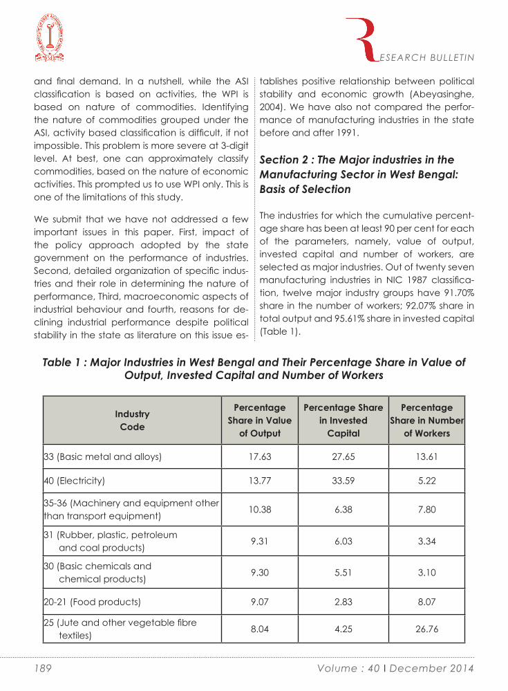
and final demand. In a nutshell, while the ASI classification is based on activities, the WPI is based on nature of commodities. Identifying the nature of commodities grouped under the ASI, activity based classification is difficult, if not impossible. This problem is more severe at 3-digit level. At best, one can approximately classify commodities, based on the nature of economic activities. This prompted us to use WPI only. This is one of the limitations of this study.
We submit that we have not addressed a few important issues in this paper. First, impact of the policy approach adopted by the state government on the performance of industries. Second, detailed organization of specific indus-tries and their role in determining the nature of performance, Third, macroeconomic aspects of industrial behaviour and fourth, reasons for de-clining industrial performance despite political stability in the state as literature on this issue es-
tablishes positive relationship between political stability and economic growth (Abeyasinghe, 2004). We have also not compared the perfor-mance of manufacturing industries in the state before and after 1991.
Section 2 : The Major industries in the Manufacturing Sector in West Bengal: Basis of Selection
The industries for which the cumulative percent-age share has been at least 90 per cent for each of the parameters, namely, value of output, invested capital and number of workers, are selected as major industries. Out of twenty seven manufacturing industries in NIC 1987 classifica-tion, twelve major industry groups have 91.70% share in the number of workers; 92.07% share in total output and 95.61% share in invested capital (Table 1).
Table 1 : Major Industries in West Bengal and Their Percentage Share in Value of Output, Invested Capital and Number of Workers
IndustryCode
Percentage Share in Value
of Output
Percentage Share in Invested
Capital
Percentage Share in Number
of Workers
33 (Basic metal and alloys) 17.63 27.65 13.61
40 (Electricity) 13.77 33.59 5.22
35-36 (Machinery and equipment other than transport equipment)
10.38 6.38 7.80
31 (Rubber, plastic, petroleum and coal products)
9.31 6.03 3.34
30 (Basic chemicals and chemical products)
9.30 5.51 3.10
20-21 (Food products) 9.07 2.83 8.07
25 (Jute and other vegetable fibre textiles)
8.04 4.25 26.76
ESEARCH BULLETIN
189 Volume : 40 I December 2014

IndustryCode
Percentage Share in Value
of Output
Percentage Share in Invested
Capital
Percentage Share in Number
of Workers
37 (Transport equipment and parts)
5.47 3.48 10.25
34 (Metal products and parts, except machinery and equipment)
2.86 1.49 2.53
28 (Paper and paper products) 2.34 1.66 2.90
23 (Cotton textiles) 2.30 1.69 5.68
32 (Non-metallic mineral products) 1.59 1.04 2.43
Total 92.07 95.61 91.70
NIC 33 contributed the highest percentage share (17.63%) in the state’s total value of output. NIC 44 has the highest share in the invested capital. NIC 25 has the highest percentage share in the number of workers. NIC 32 has the lowest share in all the three parameters.
Section 3 : Performance of Major Industries in West Bengal
Performance has been assessed on the basis of widely accepted seven indicators as stated in section 1. Year wise value of each indicator for major industry groups was calculated. Ranks of individual industry group in terms of three mac-ro variables, namely, VO, IC and NW were first found out. Similar exercise was then performed in terms of four productivity measures, namely, FP, CP, MP and LP. Ranks were also given in terms of composite productivity ratio. The best was assigned rank 1 and worst was assigned 12.
Results are given in Table 2 and Table 3. We then checked whether performance of major industries remained consistent throughout the selected time period. Kendall’s coefficient of
concordance (W) is used to find out the degree of consistency in the rankings of each industry group. Kendalls W is measured as W = 12S /[m2(n3 – n)] where, S = ∑ (Ri -R)2 ; m = number of rankers and n = number of objects to be ranked. Ri = Rank of the ith state. The average value R‾ = ½ m (n+1).
Value of W is found to be 0.7662, 0.9473 and 0.9447 with respect to value of output, invested capital and number of workers respectively.
ESEARCH BULLETIN
190Volume : 40 I December 2014

Tabl
e 2
: Yea
r Wise
Ran
k of
Maj
or In
dust
ries
in W
est B
enga
l with
Res
pect
to Th
ree
Para
met
ers
Indu
stry
co
dePa
ra-
met
ers
8182
8384
8586
8788
8990
9192
9394
9596
9798
33V
.O.
11
11
11
12
11
11
11
11
12
I.C.
11
22
12
12
22
21
22
21
21
N.W
.2
22
22
22
22
22
22
22
22
3
40V
.O.
78
88
75
43
24
52
22
22
21
I.C.
22
11
21
21
11
12
11
12
12
N.W
.7
77
77
77
76
76
66
66
66
5
35-3
6V
.O.
32
22
34
34
35
33
44
43
37
I.C.
55
33
34
44
34
43
45
53
56
N.W
.4
44
45
44
44
54
45
55
45
6
31V
.O.
56
55
67
65
53
24
33
35
74
I.C.
34
44
53
33
55
55
33
34
33
N.W
.8
89
88
88
88
98
119
99
109
9
30V
.O.
33
33
46
21
46
66
56
56
46
I.C.
43
65
45
55
43
34
54
45
44
N.W
.11
1112
1111
129
99
89
87
88
88
8
20-2
1V
.O.
45
44
53
56
62
45
65
67
63
I.C.
88
98
77
88
88
88
88
78
85
N.W
.5
55
66
55
55
45
53
44
54
2
25V
.O.
34
66
22
77
76
77
77
74
55
I.C.
77
77
88
77
76
66
77
66
79
N.W
.1
11
11
11
11
11
11
11
11
1
37V
.O.
67
77
88
88
87
88
88
88
88
I.C.
66
56
66
66
67
77
66
87
67
N.W
.3
33
33
33
33
33
34
33
33
4
34V
.O.
1010
1111
1011
119
98
99
99
910
910
I.C.
1111
1111
1111
1210
1010
99
99
1110
1110
N.W
.10
1011
129
1012
1110
1110
1011
1012
1211
11
28V
.O.
911
1010
1110
1010
1010
1010
1112
109
1011
I.C.
1010
1010
1010
1011
911
1010
1211
99
911
N.W
.9
98
910
910
1011
1211
910
1110
910
10
23V
.O.
89
99
99
911
119
1111
1010
1111
119
I.C.
99
89
99
99
119
1111
1010
1012
128
N.W
.6
66
54
66
67
67
78
77
77
7
32V
.O.
1112
1212
1212
1212
1211
1212
1211
1212
1212
I.C.
1212
1212
1212
1112
1212
1212
1112
1211
1012
N.W
.12
1210
1012
1111
1212
1012
1212
1211
1112
12
Not
e: V
.O. -
Val
ue o
f Out
put,
I.C. -
Inve
sted
Cap
ital,
N.W
. - N
umbe
r of W
orke
rs
ESEARCH BULLETIN
191 Volume : 40 I December 2014

Table 3 : Productivity Ratios for Major Industries in West Bengal
NIC Code F.P. C.P. M.P. L.P. Composite RankValue Rank Value Rank Value Rank Value Rank
33 210.95 6 0.92 11 1.59 6 1.69 5 640 3837.38 1 0.44 12 2.59 1 2.55 3 1
35-36 111.68 7 1.81 6 1.60 5 1.95 4 331 259.53 4 1.68 9 1.36 10 4.43 2 530 286.73 3 2.05 4 1.37 8 4.88 1 2
20-21 87.37 9 3.91 1 1.22 11 1.65 6 725 621.36 2 2.34 2 1.81 3 0.32 12 437 251.58 5 1.76 7 1.45 8 0.83 10 934 41.56 12 2.29 3 1.37 9 1.39 7 1028 46.99 11 1.66 10 1.68 4 0.96 8 1123 128.39 8 1.74 8 1.52 7 0.64 11 1232 61.62 10 1.84 5 2.03 2 0.87 9 8
Note: F.P. - Factory Productivity, C.P. - Capital Productivity, M.P. - Material Productivity, L.P. - Labour Productivity
On the basis of empirical analyses based on three macro variables, IC 33, IC 40, IC 35-36, IC 31 and IC 30 are identified as ‘good performing’ industries and IC 34, IC 28, IC 23, IC 32 and IC 25 as ‘bad performing’ industries. Performance in terms of productivity ratios, however, depicts a different scenario. IC 40, IC 30, IC 35-36 and IC 25 are found to be good performers. IC 23, IC 28, IC 34 and IC 37 are bad performers. Others are at median level. Some industries, namely, IC 33 and IC 31 which are found to be consistently good performing with respect to three macro-economic variables are found to be bad performers in terms of productivity ratios. This is what is expected as it has been observed that the productive efficiency of an economic unit is not fully captured either in terms of capital or labour. For example, productivity ratios of tex-tile industries with highest deployment of capital and labour are poor. Again, an improved pro-ductivity might not necessarily mean higher rate of profit. Profit being the difference between revenue and cost, a decrease in cost would be reflected in higher profit if revenue remains the same or alternately, if the rate of growth of revenue is more than the rate of declining of
cost. Empirical findings capture the industrial scenario in the state. It is observed that these good performing industries have attracted good investment. Kendall’s W value over a period of 18 years indicate that individual industry group had shown higher degree of consistency with respect to their individual ranking.
Section 4 : A Comparative Analysis of Performance
A comparative study has been made with a view to understand how the manufacturing industries in other major states in India performed during the reference period as compared to that of West Bengal. Homogeneous behaviour would imply deficiency in policy measures at the central level and heterogeneous behaviour would indicate weakness in government policy in the state level. Comparison has been made with reference to ranks based on growth rate (mean of average y-o-y growth, annual compounded growth and log linear growth) in value of output, invested capital and number of workers employed and mean of three productivity measures, namely, material, labour and capital productivity (Table 4).
ESEARCH BULLETIN
192Volume : 40 I December 2014

Table 4 : Ranks With Respect to Seven Parameters
StateV.O. I.C. N.W. M.P. L.P. C.P. Composite
RankRank Rank Rank Rank Rank RankWest Bengal 14 13 13 10 14 7 14Bihar 13 14 14 2 11 10 13Orissa 7 2 10 4 7 14 8Madhya Pradesh 2 11 8 9 5 11 12Andhra Pradesh 5 3 3 6 9 12 4Uttar Pradesh 3 4 12 5 6 13 5Maharashtra 11 7 11 7 1 8 11Tamilnadu 10 6 5 11 13 5 10Gujarat 8 1 2 12 2 6 1Karnataka 6 5 6 3 12 9 7Kerala 12 12 9 1 8 3 9Punjab 9 9 1 13 10 1 6Haryana 1 10 4 14 4 2 3Rajasthan 4 8 7 8 3 4 2
Note: V.O.- Value of Output, I.C.- Invested Capital, N.W.- Number of Workers, M.P.- Material Productivity, L.P.- Labour Productivity, C. P.- Capital Productivity
Outcome of analyses indicates that perfor-mance of manufacturing industries in West Bengal are bad compared to all other states. This indicates that during the pre and post-re-form period, unlike other states, namely, Gujarat, Maharashtra, Madhya Pradesh, Haryana and Rajasthan, industries in West Bengal, which are traditional in nature, have not modernised with adequate capital investment in order to achieve cost efficiency and competitiveness.
Section 5 : Conclusion
The aim of this research is to assess the perfor-mance of manufacturing industries in West Bengal and also to portray the vulnerable state of the West Bengal manufacturing industries as compared to those in other states of the country. Precisely, the state’s share in the country’s total value of output, invested capital and numbers of workers has not improved during the selected time period. Industries have also not performed well compared with the similar type of industries
located in other states. Conventional wisdom points toward the lag in policy upgradation to support the industrial environment. However, there may be some other reasons for deterio-rating industrial environmental scenario of the state. This claims for further research to identify the cause-effect scenario that may help identify the policy lags.
References
Ahluwalia, Isher Judge (1985), ‘Industrial Growth in India: Stagnation since the Mid-Sixties’, Oxford University Press, Oxford.
(1991), ‘Productivity and Growth in Indi-an Manufacturing’, Oxford University Press, New Delhi.
Abeyansinghe, Ranmali (2004): ‘Democ-racy, Political Stability and Developing Country Growth: Theory and Evidence’, Spring, p 17.
Balakrishnan, Pulapre and Babu, M
ESEARCH BULLETIN
193 Volume : 40 I December 2014

Suresh (2003): ‘Growth and Distribution in Indian Industry in the Nineties’, Economic and Political Weekly, September 20.
Chattopadhyay, Sadhan (2004): ‘Trends in Total Factor Productivity of Manufacturing Sector in West Bengal: a Sectoral and Temporal analysis’, Reserve Bank of India Occasional Pa-pers, vol. 25, No. 1, 2 and 3.
Das, Deb Kusum (2004), ‘Manufacturing Productivity under Varying Trade Regimes, 1980-2000’, Economic & Political Weekly, January 31.
Datta, Dilip (2012): ‘Performance of Manufacturing Industries: Interstate disparities in India’, The Journal of Industrial Statistics, vol. 1, no. 1, pp. 97 – 110.
Dholakia, Ravindra (2014): ‘Relative Growth performance of Gujarat: A comment on the recent debate’, Economic and Political Weekly, vol. 49, no. 18, May 3.
Golder, B N (1986), ‘Productivity Growth in Indian Industry’, Allied Publishers, Delhi.
Ghatak, Maitreesh and Roy, Sanchari (2014): ‘Did Gujarat switch to a higher growth trajectory relative to India under Modi’, Econom-ic and Political Weekly, vol. 49, no. 18, May 3.
Joseph, Mathew (2004), ‘Performance of the Northern States: A Comparative Analysis’, Economic and Political Weekly, February 7.
Kaldor, N (1958), ‘Capital Accumulation and Economic Growth, reprinted in Further Essays on Economic Theory’, Duckworth, 1978, London
Khasnabis, Ratan (2008): ‘The Economy of West Bengal’, Economic and Political Weekly, vol. 43, no. 52, December 27.
Marjit, Sugata (2014): ‘On UPA vs NDA; Gujarat vs Rest of India: Myth and Reality’, Eco-nomic and Political Weekly, vol. 49, no. 18, May 3.
Nagaraj, R and Pandey, Shruti (2013): ‘Have Gujarat and Bihar outperformed the rest
of India? A statistical note’, Economic and Politi-cal Weekly, vol. 48, no. 39, September 28.
Nagaraj, R (2014): ‘Gujarat’s Economic Performance: A Response’, Economic and Politi-cal Weekly, vol. 49, no. 18, May 3.
Siddharthan, N S and K Lal (2003), ‘Liber-alisation and Growth of Firms in India’, Economic and Political Weekly, 38(20).
ESEARCH BULLETIN
194Volume : 40 I December 2014

1. Introduction
Profitability may be defined as the ability of a given investment to earn a return from its use. Greater the profit, the more efficient is the busi-ness and vice versa. Thus, profit is the engine that drives the wheel of business enterprise. It is the primary measure of overall success and neces-sary condition for the survival and growth of an enterprise. Further, profitability analysis is useful for the following reasons:
►► Routine pricing policy.
►► Impact of price increase or price decrease.
►► Selection of product mix.
►► Project evaluation.
►► Valuation of goodwill and shares.
Profit rate in terms of returns on shareholders equity being one of the popular measure of financial performance, indicates the financial stability and earning capacity of an enterprise. It plays a dual role by attracting fresh investment on the one side and generating internal source of finance on the other side in the investment process of an economy.
Returns on Shareholders Equity of Select Industries in Liberal Economic Scenario: Empirical Evidence From India
Sudipta GhoshAbstract
In the name of liberalization, various reform measures were introduced to make the Indian industries efficient and to achieve growth and development in the economy. The present paper is an attempt to empirically examine the profit rate in terms of returns on shareholders equity of select industries during the period 2004-05 to 2012-13. The findings of the study indicate that returns on shareholders equity in majority of the selected industries did not rise over the time period. The industry as a whole has recorded an average profit rate of 24% during the entire study period. On the average, auto & ancillary industry has posted highest profit rate (103%), while chemical and paper industry have posted lowest profit rate (5%) during the whole study period. The sub-period analysis shows that economic recession has negative impact on the generation of profit.The study concludes that liberalization measures should be further strengthened in order to achieve better efficiency, productivity, and profitability for the selected industries in particular and other industries in general.
Keywords
Profitability; Profit Rate; Returns on Shareholders Equity; Liberalization; Dispersion.
ESEARCH BULLETIN
195 Volume : 40 I December 2014

2. Review of Past Studies
For presenting brief reviews of literature, the available empirical studies have been grouped into Indian studies and Foreign studies.
2.1 Indian Studies
Mohanakumar, P.S. (1996), in his study pointed out that profitability of textile industry in Kerala was generally low when compared to that in other major industries during the period 1982-83 to 1991-92. It was also observed that selected spinning mills depended excessively on debt capital and their internal resource mobilization was very poor due to low level of general reserve.
Dasgupta, Debajyoti (2001), evaluated the profitability performance of six selected public sector banks during the period 1986 to 1996-97. It was found that Vijaya Bank and Corporation Bank had attained better results compared to that of other banks selected in the study. More-over, both the banks had secured better results in five years out of ten years as compared to that of total public sector banks.
Rej, Debasis and Sur, Debasish (2001), attempted to measure the profitability of Cadbury India Ltd. during 1987-88 to 1996-97 by analyzing the de-gree of relationship among various profitability ratios through multiple correlation and multiple regression method.
The study concluded that the profitability per-formance of the selected company in terms of gross profit ratio, net profit ratio and return on investment ratio was not stable during the study period. Moreover, the study revealed both positive and negative associations on the inter-relation between company’s position and performance and profitability.
Pandey, R. and Bandyopadhyaya, S. (2003), in their study on cost-volume-profit analysis of 27 public sector banks revealed that profitability
was influenced by several factors namely interest earned, interest paid, operating cost, and other income. The study concluded that reduction in operating cost was the most significant factor for increased profitability of the selected banks under study.
Misra, D.P. and Mishra, P.K. (2006), analyzed the factors influencing profitability of Orissa State Warehousing Corporation (OSWC) during the period 1985-86 to 2002-03. Multiple regression technique was employed to analyze the factors influencing the profitability of OSWC. The study found that operating cost, liquidity, and fixed assets turnover were the major factors that influ-enced profitability of OSWC to a great extent.
Selvi, A. Manor and Vijayakumar, A. (2007), at-tempted to examine the trends in rates of profit of selected companies in the Indian automobile industry over the period 1991-92 to 2003-04. The study revealed that most of the Indian automo-bile companies had a tendency for profit rates to fall over a long period. Furthermore, time ex-plained this fall in profit rates at various degrees.
Ghosh, Sudipta (2012), attempted to empirically examine the impact of profitability performance in the liberalized Indian electric power industry with reference to selected central public sector power companies during the period 1998-99 to 2007-08.
The findings of the study revealed that profit-ability performance of the selected companies had significantly improved (i.e., positive impact) during the period under study. The results should therefore encourage for further investment, particularly by the private players in order to augment power generating capacity addition in the sector.
2.2 Foreign Studies
Abdurahman, A. et. al (2003), examined the firm’s size - profitability relationship of electrical
ESEARCH BULLETIN
196Volume : 40 I December 2014

contractors of U.S. during the period 1985 to 1996. The study found that small, medium, and large firms were significantly different from each other in terms of their profit rate. The indicator model which was developed in the study, pre-dicted 76% of the year 1996 response variable, profitability correctly.
Oberholzer, M. and Warthuizen, G. Van Der (2004), examined the profitability and efficiency of ten regional offices of one of South Africa’s largest banks for a period of 36 consecutive months. The study found that there was no signif-icant relationship between technical efficiency and the conventional profitability and efficiency measurements. Further, region ten had the high-est technical efficiency and profitability during the period under study.
Eljelly, Abuzar M.A. (2004), empirically examined the relationship between liquidity and profitabili-ty on a sample of joint stock companies in Saudi Arabia. The study found significant negative relationship between liquidity and profitability. At the industry level, cash conversion cycle was more important that affected profitability.
Abu-Tapanjeh, A.M. (2006), examined the rela-tionship of firm structure and profitability of 48 Jordanian industrial companies during 1995 to 2004, listed in the American Stock Exchange. The empirical findings of the study revealed that firm structure emerged as an important factor affecting profitability. The study further indicated that a weak relationship existed between some of the independent variables and profitability (except for debt ratio).
Jonsson, Bjarni (2007), attempted to examine the profitability performance of Icelandic firms in relation to their size with reference to fisheries and fish processing, banks and civil engineering consulting firms during the period 2000 to 2004. The researcher found that size had no statistically significant effect on profitability. The study further
revealed a weak inverse relationship between size and profitability for all the firms (except fish-eries and fish processing in 2004).
2.3 Research Gap
While reviewing the past studies as stated above, it is observed that these studies are fraught with some limitations. These are ascribed to limited sample size and methodology used. In the matter of sample selection, some studies have considered sample from a few specific industries. Hence, the present study may be considered as first time attempt in the area covered under study.
3. Statement Of The Research Problem
Since 1991, several reform measures were intro-duced in India in the name of liberalization for growth and development of the economy. In the liberal economic scenario, the foreign players are allowed to operate in the Indian domes-tic market. This lead to a different economic environment in which, the Indian companies are to perform efficiently in order to survive in the face of this increasing competition.
In this backdrop, the present study is an attempt to examine the returns on shareholders equity of selected Indian industries in the liberal economic scenario. 4. Research Objectives
The main objective of the present study is to empirically examine the profit rate performance in terms of returns on shareholders equity of se-lected Indian industries during the pre-recession and post-recession phase. To attain this main objective, the following incidental objectives are sought to be achieved:
►► To examine the trends in profit rate perfor-mance of the selected industries.
ESEARCH BULLETIN
197 Volume : 40 I December 2014

►► To examine the profitability performance of the selected industries on the basis of “Return on Shareholders Equity/Funds (ROSE).
►► To examine the dispersion in profit rate performance of the selected industries.
►► To examine whether there exist significant differences in average profit rate performance between the sample companies within each selected industry.
►► To compare the profit rate performance of each selected industry with the aggregate industry performance.
5. Research Hypothesis
In conformity with the above objectives, the following testable hypothesis have been formu-lated:
►► Profit rate trends of the selected industries have a tendency to rise over time.
►► Profit rate performance of the selected
companies within each industry has significant bearing on the aggregate industry perfor-mance.
►► Profit rate performance of each selected industry is not moving with the aggregate indus-try performance.
6. Data, Sample And Methodology
6.1 Sample Design and Sample Selection
Based on the availability of data, sixteen industries have been selected covering both manufacturing sector and service sector. For each industry, three sample companies have been chosen on the basis of random sampling method. This leads to a total sample size of forty eight companies.
The list of selected industries and the sample companies falling within each industry is present-ed in Table – I below:
ESEARCH BULLETIN
Table I : List of Selected Industries and the Sample Companies within each Industry
S.L. No. Industries Sample Companies
1 Infrastructure: Larsen & Toubro Ltd. Nagarjuna Construction Co.Ltd. Hindusthan Construction Ltd.
2Auto and Ancillaries:
Tata Motors Ltd. Hero Honda Motors Ltd. Ashok Leyland Ltd.
3 Cement: Ultratech Cement Ltd. J.K. Cements Ltd. J.K. Lakshmi Cement Ltd.
4 Chemicals:United Phosphorus Ltd. Philips Carbon Black Ltd. Bombay Deying & Mgf. Co. Ltd.
5 Diversified:Grasim Industries Ltd. Voltas Ltd. Aditya Birla Nuvo Ltd.
198Volume : 40 I December 2014

S.L. No. Industries Sample Companies
6 Electronics:Comptron Greaves Ltd. Blue Star Ltd. Whirlpool of India Ltd.
7 Fertilizers:Tata Chemicals Ltd. Chambal Fertilizers & Chemicals Ltd. Nagarjuna Fertilizers and Chemicals Ltd.
8Fast Moving Consumer Goods:
Nirma Ltd. Britannia Industries Ltd. Dabur India Ltd.
9Information Technology:
Tech Mahindra Ltd. CMC Ltd. Tata Consultancy Services Ltd.
10 Jewelry: Su-Raj Diamond & Jewelry Ltd. Gitanjali Gems Ltd. Asian Star Co. Ltd.
11 Oil: Hindusthan Petroleum Corporation Ltd. Reliance Industries Ltd. Indian Oil Corporation Ltd.
12 Paper: Ballarpur Industries Ltd. Tamil Nadu Newsprint & Papers Ltd. Andhra Pradesh Paper Mills Ltd.
13 Steel: Tata Steel Ltd. JSW Steel Ltd. Jindal Stainless Ltd.
14 Textile: The Arvind Mills Ltd. Alok Industries Ltd. Raymond Ltd.
15 Transport: Container Corporation of India Ltd. Transport Corporation of India Ltd. ABG Shipyard Ltd.
16 Trading: MMTC Ltd. Gail (India) Ltd. Adani Enterprises Ltd.
ESEARCH BULLETIN
6.2 Study Period
The study period has been selected from the fi-nancial year 2004-05 to the financial year 2012-13. Thus, a span of 9 years for 48 sample companies gives a cross-sectional data set of 432 firm-year observations. Further, to assess the impact of recession on profitability, the entire study period
(2004-05 to 2012-13) has been sub-divided into two phases: (i) pre-recession phase (2004-05 to 2007-08) and (ii) post-recession phase (2008-09 to 2012-13).
6.3 Data Source
For the present study, secondary data have
199 Volume : 40 I December 2014

been used which are collected mainly from the published annual reports of the sample compa-nies.
6.4 Methodology
After collection of necessary data, these are suitably re-arranged, classified, tabulated, and computed as per requirements of the study. Necessary calculations have been done with the help of SPSS and Microsoft Excel software packages.
To examine the trends in profit rate performance of the selected industries, return on shareholders equity / funds i.e., [(Net Profit after Tax ÷ Capital Employed) × 100] has been used in the study, since it is a better indicator of long-term profit-ability. For this purpose, linear regression model has been applied which is shown below:
P = a + β t + e -------------------------------eq. (1)
Where: P = return on shareholders equityt = timea and b = parameters indicating intercept and co-efficient respectivelye = error term
The significance of beta coefficient has been tested by the popular ‘t’ test. Further, to detect the problem of autocorrelation, Durbin-Watson d (D.W.) statistic is applied in the study. The
presence of autocorrelation (if any) is adjusted by the technique of first difference operator. The D.W. statistic is computed as follows:
t = n t = n d = Σ (Ût - Ût – 1)2 ÷ Σ Û2
t ----------eq. (2) t = 2 t = 1
The above ratio indicates the sum of squared differences in successive residuals to the RSS. As earlier stated, return on shareholders equity/funds is used to examine and analyze
the profitability performance of the selected industries. Furthermore, the dispersion in profit rate performance has been measured by coefficient of variation (C.V.) i.e., [(Standard Deviation ÷ Mean) × 100]. For this purpose, it has been arbitrarily divided into relatively stable (C.V. with value up to 25%), moderately fluctuating (C.V. lying between 25.1% and 50%), highly fluctuating (C.V. lying between 50.1% and 75%), and erratically fluctuating (C.V. above 75%) [Selvi and Vijaya, 2007].
To examine whether there exist significant variations in the average profit rate performance between the sample companies within each selected industry, the technique of One-Way Analysis of Variance (ANOVA) has been applied in the study.
Since ANOVA is a robust departure from normality, Kruskal-Wallis test (H Test) has also been employed in the study. The Kruskal Wallis test uses the χ2 – test to test the null hypothesis. The test statistic is given by:
K H =12 ÷[ N (N + 1) ] Σ [ R2
j ÷ nj ] - 3 (N + 1) --eq. (3) j=1 Where: Rj = sum of the ranks of the sample jnj = size of the sample jj = 1, 2, 3, ……., kN = size of the pooled sample (n1 + n2 + ……. + n K)
H follows χ 2 – distribution with (k-1) degrees of freedom.
Finally, to compare the profit rate performance of each industry with the total industry perfor-mance, Man-Whitney U-Test has been applied in the study. As the size of the second sample (n2) is more than 8 in our study, we have normal approximation to the given data.
The test statistic is shown below:
ESEARCH BULLETIN
200Volume : 40 I December 2014

ZU = (U - μU) ÷ σU -------------------------eq. (4)
Where: U = (n1 n2 ) + [{n1 (n1 + 1)} ÷ 2] – R1
μU = (n1 n2) ÷ 2σU = [{n1 n2 (n1 + n2 + 1)} ÷ 12]1/2
R1 = Sum of the ranks of the observations of the first sample.n1 and n2 = size of the first sample and second sample respectively.
7. Empirical Findings And Analysis
7.1 Profit Rate (i.e., Return on Shareholders Equity) Trends in Selected Industries
From Table-II, it is observed that there is no definite profit rate trends in the selected industries (except fast moving consumer goods, jewelry, and oil) as the results are found to be statistically
insignificant during the whole study period. Fast moving consumer goods and oil industry indicates a declining trend in profitability, while jewelry industry shows a strong tendency in profitability to increase over the time period which is statistically significant either at 1% or 5% level. In terms of sub-period performances (i.e., pre-recession phase and post-recession phase), majority of the industries show no definite trend in profitability. During the pre-recession phase, industries like cement (0.08), chemicals (0.01), and electronics (0.10) indicate an increasing trend in profitability, while in the post-recession phase, only fertilizers (0.02) show an increasing trend of the same.Overall, profit rate performance (i.e., returns on shareholders equity) in majority of the selected industries did not rise over the time period, thereby leading to the rejection of the first hypothesis of the study.
ESEARCH BULLETIN
Table – II : Trends in Profit Rate Performance (represented by Return on Shareholders Equity)
of Selected Industries during 2004-05 to 2012-13
Industry
R2 b (beta co-efficient) D.W.
Pre Rece-ssion Phase
PostRece-ssion Phase
Whole Period
PreRece-ssion Phase
PostRece-ssion Phase
Whole Period
PreRece-ssion Phase
PostRece-ssion Phase
Whole Period
Infrastru-cture
0.70 0.66 0.360.01i
(2.160)-0.0288
(-2.393)-0.008i
(-1.981)2.07 2.18 1.33
Auto & Ancillary
0.10 0.41 0.35-0.10i
(-0.460)-0.22i
(-1.437)-0.11i
(-1.948)2.91 2.79 2.62
Cement0.92 0.17 0.01
0.08888
(4.940)-0.01i
(-0.781)0.01i
(0.121)3.27 2.52 1.20
Chemicals0.80 0.29 0.01
0.0188 (2.828)
0.03i (1.103)
0.01i (0.144)
2.62 1.63 2.48
Diversified0.97 0.17 0.01
0.10888 (7.542)
-0.04i (-0.793)
0.01i (0.137)
3.40 2.41 1.77
201 Volume : 40 I December 2014

Industry
R2 b (beta co-efficient) D.W.
Pre Rece-ssion Phase
PostRece-ssion Phase
Whole Period
PreRece-ssion Phase
PostRece-ssion Phase
Whole Period
PreRece-ssion Phase
PostRece-ssion Phase
Whole Period
Electronics0.86 0.77 0.07
0.10888 (3.559)
-0.0888
(-3.196)0.01i
(0.728)2.34 2.75 0.75
Fertilizers0.69 0.94 0.26
0.03i (2.099)
0.02888 (7.000)
0.01i (1.563)
2.14 2.53 2.63
Fast Moving Consumer Goods
0.67 0.01 0.47-0.28i
-2.017)-0.01i
(-0.024)-0.0988
(-2.502)2.02 1.83 1.27
Information Technology
0.42 0.01 0.410.03i
(1.197)0.01i
(0.162)0.03i
(2.183)3.37 2.33 2.26
Jewelry1.00 0.17 0.67
0.01i (0.082)
0.01i (0.792)
0.01888 (3.743)
1.50 2.13 1.67
Oil0.01 0.01 0.47
-0.01i
-0.077)0.01i
(0.002)-0.0188
(-2.500)3.21 1.76 2.72
Paper0.60 0.42 0.44
0.01i (1.732)
-0.02i
(-1.462)-0.01i
(-2.360)2.23 2.94 2.23
Steel0.95 0.10 0.01
-0.03888
-5.966)0.02i
(0.573)0.01i
(0.077)3.27 2.26 1.92
Textile0.61 0.30 0.37
-0.08i
(-1.755)0.01i
(1.140)-0.02i
-2.027)2.64 2.70 1.57
Transport1.00 0.03 0.06
-0.01i
-0.002)-0.01i
(-0.311)-0.01i
-0.664)1.00 1.95 2.07
Trading0.08 0.23 0.29
-0.01i
(-0.411)-0.01i
(-0.933)-0.01i
-1.690)3.07 2.96 2.97
Whole Industry 0.09 0.29 0.35 -0.01i
-0.430)
-0.02i
(-1.113)
-0.01i
-1.953) 2.13 2.82 2.71
Key Notes: *** marked values indicate significant at 1% level (2–tailed); ** marked values indicate significant at 5% level (2–tailed); i marked values indicate insignificant; Figures in the brackets indicate ‘t’ value; D.W. indicates Durbin – Watson d statistic.
ESEARCH BULLETIN
202Volume : 40 I December 2014

Table –II further reveals that the value of ‘b’ assumes different values for different industries. This implies that profit rate performance of different industries moves at different rates over the period under study. However, profit rate performance for the whole industry is found to be statistically insignificant during the whole period as well as during the two sub-periods.
7.2 Profitability (i.e., Return on Shareholders Equity) Analysis of the Selected Industries
Profitability performance of the selected industries has been examined by Return on Shareholders Equity (ROSE), since it is a better indicator of long term measure of profitability.
From Table – III, it is observed that on the average, auto & ancillaries industry shows highest profit rate (103%), while chemicals and paper industry indicates lowest profit rate (5%) during the whole study period. On the average, the whole industry
reveals a profit rate of 24% during the entire study period. It is further observed from Table – III that out of 16 industries, only 4 industries i.e., auto & ancillaries (103%), diversified (30%), fast moving consumer goods (57%), and information technology (54%) have an average profit rate above the average profit rate of the whole industry during the entire period under study.
The sub-period analysis shows that out of 16 industries, the average profit rate performances in 10 industries (i.e., infrastructure, auto & ancillaries, cement, chemicals, fast moving consumer goods, oil, paper, textile, transport, and trading) are found to be higher in the pre-recession phase as compared to that of the post-recession phase. This implies that economic recession has negative impact on the generation of profit during the period under study. On the average, the whole industry also shows higher profit rate in the pre-recession phase in comparison to that of the post-recession phase.
ESEARCH BULLETIN
203
Table – III : Profitability Performance (represented by Return on Shareholders Equity) of Selected Industries during 2004-05 to 2012-13
(Figures in %)
Year →Industry↓
Pre-Recession Phase Post-Recession Phase Average
2004-05
2005-06
2006-07
2007-08
2008-09
2009-10
2010-11
2011-12
2012-13
Pre-Recession Phase
Post-Recession Phase
Whole Period
Infrastr-ucture
14 13 15 18 13 17 13 08 07 15 12 13
Auto & Ancillary
146 145 64 141 86 179 73 53 37 124 86 103
Cement 04 06 20 25 14 16 06 10 12 14 12 13
Chemicals 05 06 06 09 -12 08 10 09 03 07 04 05
Diversified 16 22 37 43 23 55 34 17 22 30 30 30
Electronics 05 11 15 36 36 46 26 18 12 17 28 23
Volume : 40 I December 2014

Year →Industry↓
Pre-Recession Phase Post-Recession Phase Average
2004-05
2005-06
2006-07
2007-08
2008-09
2009-10
2010-11
2011-12
2012-13
Pre-Recession Phase
Post-Recession Phase
Whole Period
Fertilizers 08 08 09 17 08 10 12 12 14 11 11 11
Fast Moving Consumer Goods
142 67 46 57 48 44 21 39 50 78 40 57
Information Technology
43 50 44 53 61 63 57 45 73 48 60 54
Jewelry 03 04 05 06 06 07 05 06 08 05 06 06Oil 16 11 16 14 08 11 12 09 09 14 10 12Paper 06 07 07 07 06 06 05 -05 02 07 03 05
Steel 21 17 16 11 07 14 19 33 08 16 16 16
Textile 31 04 09 03 01 -01 01 06 02 12 02 06
Transport 18 17 16 15 18 18 12 15 18 17 16 16
Trading 12 19 11 12 12 11 10 12 10 14 11 12Whole
Industry31 25 21 29 21 32 20 18 18 27 22 24
7.3 Dispersion in Profit Rate Performance (in terms of Return on Shareholders Equity) of the Selected Industries
The industry-wise dispersion in profit rate performance (measured by coefficient of variation) is shown in Table – IV below:
Table – IV : Dispersion in Profit Rate Performance (represented by Return on Shareholders Equity) of Selected Industries during 2004-05 to 2012-13
Industry
Pre-Recession Phase
(2004-05 to 2007-08)
Post-Recession Phase
(2008-09 to 2012-13)
Whole Period(2004-05 to
2012-13)
C.V. (%) C.V. (%) C.V. (%)Infrastructure 13.33 33.33 30.77
Auto & Ancillary 32.26 63.95 48.54
Cement 71.43 33.33 53.85
ESEARCH BULLETIN
204Volume : 40 I December 2014

Industry
Pre-Recession Phase
(2004-05 to 2007-08)
Post-Recession Phase
(2008-09 to 2012-13)
Whole Period(2004-05 to
2012-13)
C.V. (%) C.V. (%) C.V. (%)Chemicals 28.57 225.00 140.00
Diversified 43.33 50.00 43.33
Electronics 76.47 50.00 60.87
Fertilizers 36.36 18.18 27.27
Fast Moving Consumer Goods 56.41 30.00 59.65
Information Technology 10.42 16.67 18.52
Jewelry 20.00 16.67 33.33
Oil 14.29 20.00 25.00
Paper 14.29 166.67 80.00
Steel 25.00 68.75 50.00
Textile 108.33 150.00 166.67
Transport 5.88 18.75 12.50
Trading 28.57 9.09 25.00
Whole Industry 14.81 27.27 25.00
ESEARCH BULLETIN
The Coefficient of Variation (C.V.) indicates the extent of variation in actual values of profit rate of each industry from its mean value of the series. Accordingly, higher value of C.V. indicates high-er fluctuation in profit rate series of the respective industries and vice versa.
From Table – IV, it is observed that transport industry with a C.V. of 12.50% reflects lowest variation in profit rates, while textile industry with a C.V. of 166.67% has experienced largerdisper-sion in profit rates over entire the study period. Almost, all the industries (except information technology, oil, transport, and trading) have experienced higher dispersion in profit rate series as compared to that of the whole industry. Table – IV further reveals that the rate of fluctuation in profit rate series has varied widely among the industries selected in the study.
During the whole study period, we have found
that 4 industries out of 16 industries (25%) have witnessed relatively stable performance in profit rate series during the period under study. These industries include information technology, oil, transport, and trading. 6 out of 16 industries (37.5%) have experienced moderate fluctuation in profit rate series. These industries are infra-structure, auto & ancillaries, diversified, fertilizers, jewelry, and steel. Again 3 out of 16 industries (18.75%) have registered high fluctuation in profit rate series. These industries comprises of cement, electronics, and fast moving consumer goods. The remaining 3 industries (i.e., chemicals, paper, and textile) indicate erratical fluctuation in profit rate series. The industry as whole shows relatively stable performance (25%) in profit rate series during the entire study period.
In terms of sub-period performances, majority of the industries (i.e., 10 out of 16 industries) and the industry as a whole have shown higher fluctua-
205 Volume : 40 I December 2014

tion in profit rate series during the post-recession phase as compared to that of the pre-recession phase.
7.4 Variation in Average Profit Rate Performance (represented by Return on Shareholders Equity) between Sample Companies within each Selected Industries
To examine whether there exist significant variation in average profit rate performance between the sample companies within each
industry selected in the study, the technique of One-Way ANOVA has been applied.
From Table – V, it is evident that out of 16 industries, 11 industries i.e., infrastructure, auto & ancillaries, diversified, fertilizers, fast moving consumer goods, information technology, oil, paper, steel, transport, and trading show significant results. These results indicate that there exist significant differences in average profit rate between the sample companies within each industry. In the remaining 4 industries, the results are observed to be statistically insignificant.
ESEARCH BULLETIN
Table – V : One-Way Analysis of Variance (ANOVA) between Sample Companieswithin each Selected Industries during 2004-05 to 2012-13
Industry Source of Variation Sum of Squares D.F. Mean
Square F-Ratio
InfrastructureBetween Groups
Within Groups
0.36
0.07
2
24
0.180
0.00360.00***
Auto & AncillaryBetween Groups
Within Groups
32.91
18.07
2
24
16.455
0.75321.85***
CementBetween Groups
Within Groups
0.04
0.15
2
24
0.020
0.0063.33 i
ChemicalsBetween Groups
Within Groups
0.01
0.24
2
24
0.005
0.0100.50 i
DiversifiedBetween Groups
Within Groups
0.53
0.91
2
24
0.265
0.0386.97***
ElectronicsBetween Groups
Within Groups
0.11
0.95
2
24
0.055
0.0401.38 i
FertilizersBetween Groups
Within Groups
0.18
0.08
2
24
0.090
0.00330.00***
206Volume : 40 I December 2014

Industry Source of Variation Sum of Squares D.F. Mean
Square F-Ratio
Fast Moving Consumer Goods
Between Groups
Within Groups
3.53
6.27
2
24
1.7650.261
6.76***
Information TechnologyBetween Groups
Within Groups
0.84
1.34
2
24
0.420
0.0567.50***
JewelryBetween Groups
Within Groups
0.00
0.01
2
24
0.000
0.0010.00 i
OilBetween Groups
Within Groups
0.02
0.04
2
24
0.010
0.0025.00**
Paper Between Groups
Within Groups
0.04
0.03
2
24
0.020
0.00120.00***
SteelBetween Groups
Within Groups
0.62
0.52
2
24
0.310
0.02214.09***
TextileBetween Groups
Within Groups
0.02
0.70
2
24
0.010
0.0290.34 i
TransportBetween Groups
Within Groups
0.10
0.06
2
24
0.050
0.00316.67***
TradingBetween Groups
Within Groups
0.09
0.06
2
24
0.045
0.00315.00***
Key Notes: *** marked values indicate significant at 1% level, ** marked value indicates significant at 5% level, i marked values indicate insignificant
ESEARCH BULLETIN
207
To overcome the precondition of normal distri-bution in case of ANOVA, we have also applied Kruskal Wallis test. Table – VI reveals that there exist significant differences between the sample companies within each industry selected in the study. The results are significant at 1% level in all the industries.
These results (i.e., ANOVA and Kruskal Wallis test) indicate that profit rate performance in terms of returns on shareholders equity of the sample companies within each selected industry has significant bearing on the aggregate industry performance. This also leads to the acceptance of the second hypothesis of the study.
Volume : 40 I December 2014

Table – VI : Kruskal Wallis Test between Sample Companies within each
Selected Industries during 2004-05 to 2012-13
Industry D.F.Computed
Value of Chi-Square
Infrastructure 02 48.48***Auto & Ancillary 02 49.00***Cement 02 27.50***Chemicals 02 24.38***Diversified 02 42.14***Electronics 02 24.90***Fertilizers 02 49.93***Fast Moving Consumer Goods 02 44.78***
Information Technology 02 38.67***
Jewelry 02 28.38***Oil 02 33.13***
Industry D.F.Computed
Value of Chi-Square
Paper 02 32.30***Steel 02 43.32***Textile 02 15.08***Transport 02 42.24***Trading 02 42.24***
Key Notes: *** marked values indicate significant at 1% level
7.5 Comparison of Profit Rate Performance (i.e., Returns on Shareholders Equity) of each Selected Industry with Aggregate Industry Performance
In this respect, Man-Whitney U-Test has been applied in order to compare the profit rate performance of each industry with that of the aggregate industry performance.
Table – VII : Man-Whitney U-Test for Comparison of Profit Rate Performance (represented by Returns on Shareholders Equity) of each Industry with Aggregate
Industry Performance during 2004-05 to 2012-13
Industry Zu Values Results
Infrastructure 3.49 H0 rejected at 1% level (2-tailed)Auto & Ancillary -3.58 H0 rejected at 1% level (2-tailed)Cement 2.87 H0 rejected at 1% level (2-tailed)Chemicals 3.58 H0 rejected at 1% level (2-tailed)Diversified -0.93 H0 acceptedElectronics 0.57 H0 acceptedFertilizers 3.58 H0 rejected at 1% level (2-tailed)Fast Moving Consumer Goods -3.14 H0 rejected at 1% level (2-tailed)Information Technology -3.58 H0 rejected at 1% level (2-tailed)Jewelry 3.58 H0 rejected at 1% level (2-tailed)Oil 3.58 H0 rejected at 1% level (2-tailed)Paper 3.58 H0 rejected at 1% level (2-tailed)
ESEARCH BULLETIN
208Volume : 40 I December 2014

Industry Zu Values Results
Steel 2.25 H0 rejected at 5% level (2-tailed)Textile 2.92 H0 rejected at 1% level (2-tailed)Transport 3.22 H0 rejected at 1% level (2-tailed)Trading 3.40 H0 rejected at 1% level (2-tailed)
ESEARCH BULLETIN
From Table – VII, it is observed that all the indus-tries (except diversified, and electronics) are not moving with the aggregate industry perfor-mance in terms of profit rate, thereby leading to the acceptance of the third hypothesis of our study. This is indicative of the fact that industry specific factors are strong enough in determin-ing their individual performance.
8. Conclusions And Policy Implication
In relation to the main objective of the study, it may be concluded that profit rate performance (i.e., returns on shareholders equity) in majority of the selected industries shows no specific trend during the period under study. Overall, the profit rate performance in majority of the selected industries did not rise over the time period.On the average, majority of the selected industries have shown higher profit rate in the pre-recession phase as compared to that of the post-recession phase, which implies that economic recession has negative impact on the returns of shareholders equity during the period under study. Only, 25% of the selected industries have experienced relatively stable profit rate performance, while the remaining industries have experienced either moderate or high or erratical fluctuations of the same during the whole study period. Moreover, 62.5% of the se-lected industries have shown higher fluctuation in profit rate during the post-recession phase as compared to that of the pre-recession phase.
The average profit rate performance has varied among the sample companies within each
industry, thereby having significant impact on aggregate industry performance. Finally, profit rate performance in most of the industries is not moving with the aggregate industry per-formance, which implies that industry specific factors are strong enough in determining their performance.
In view of the above findings, it is suggested that liberalization measures should be further strengthened so as to achieve better efficiency, productivity, and profitability for the selected industries in particular and other industries in general.
9. Limitations And Scope For Further Re-search
The study is based on secondary data i.e., pub-lished annual financial reports of the selected industries. So, it is subject to all the limitations that are inherent in secondary data. Apart from it, the study is limited to nine years only.
In spite of these limitations, further research may be undertaken by including more sample com-panies within each industry, longer time period and using other measures like return on assets, market value added etc.
References
Abdurahman, A. et. al. (2003): “Indicator Variables Model of Firm’s Size-Profitability Rela-tionship of Electrical Contractors using Financial and Economic Data”, Journal of Construction Engineering and Management, Vol. 129, No.2.
209 Volume : 40 I December 2014

Abu-Tapanjeh, A.M. (2006): “An Em-pirical Study of Firm Structure and Profitability Relationship – The Case of Jordan”, Journal of Economic and Administrative Sciences, Vol.22, No.1, June Issue.
Chandra, Prasanna (2011): Financial Management – Theory and Practice, 8th Edition, Tata McGraw Hill Education Private Limited, New Delhi.
Dasgupta, Debajyoti (2001): “Profitability of Indian Public Sector Banks in the light of Liber-alization of Indian Economy – An Overview”, The Management Accountant, June Issue.
Eljelly, Abuzar M.A. (2004): “Liquidity – Profitability Trade Off – An Empirical Investigation in an Emerging Market”, International Journal of Commerce and Management, Vol.14, Issue 2.
Ghosh, Sudipta (2011): “Performance Evaluation through Cash Management”, Indian Journal of Accounting, Vol. XLII (1), December Issue.
Ghosh, Sudipta (2012): “Profitability Impact Assessment in Selected Indian Central Public Sector Power Companies - Empirical Evidence on Aggregation”, The Management Accountant, Vol.47 No 7, July Issue.
Jonsson, Bjarni (2007): “Does Size Matter? The Relationship between Size and Profitability of Icelandic Firms”, Timarit Um Felagsvisinde, Haskolinn A Bifrost. Bifrost University, Vinnugrin (Working Paper).
Khan, M.Y. and Jain, P.K. (2011): Fi-nancial Management – Text and Problems, 6th Edition, Tata McGraw – Hill Publishing Company Ltd., New Delhi.
Kothari, C.R. (2011): Research Methodol-ogy – Methods and Techniques, 2nd Edition, Tata McGraw – Hill Publishing Company Ltd., New Delhi.
Mohanakumar, P.S. (1996): “Inter-Sec-
toral Differences in Profitability – A Case Study of Spinning Mills in Kerala”, The Management Accountant, February Issue.
Misra, D.P. and Mishra, P.K. (2006): “Factors Influencing Profitability of OSWC: An Economic Analysis”, The Management Accoun-tant, December Issue.
Oberholzer, M. and Westhuizen, G. Van Der (2004): “An Empirical Study on Measuring Efficiency and Profitability of Bank Regions”, Meditari Accountancy Research, Vol. 12, No.1.
Pandey, R. and Bandyopadhyaya, S. (2003): “Cost-Volume-Profit Analysis and Bank’s Performance – A Case Study of Public Sector Banks”, The Management Accountant, June Issue.
Panneerselvam, R. (2004): Research Methodology, Eastern Economy Edition, Pren-tice-Hall of India Private Limited, New Delhi.
Published Annual Reports of the Select-ed Companies from 2004-05 to 2012-13.
Rej, Debasis and Sur, Debasish (2001): “Profitability Analysis of Indian Food Products In-dustry - A Case Study of Cadbury India Ltd”, The Management Accountant, November Issue.
Rajamohan, S. and Vijayaragavan, T. (2008): “Production Performance of Madras Cements Limited and that of All Cement Units in India – A Comparative Analysis”, The Manage-ment Accountant, April Issue.
Selvi, A. Manor and Vijayakumar, A. (2007): “Structure of Profit Rates in Indian Automobile Industries – A Comparison”, The Management Accountant, October Issue.
www.moneycontrol.com.
ESEARCH BULLETIN
210Volume : 40 I December 2014

Introduction
Performance Management: Performance Management is nothing but managing the performance. In Other words PM is ‘managing translation of plans into results i.e. execution’ It is like an umbrella which includes methodologies, processes, tools, controls, systems etc.
Balanced Scorecard: A new approach to stra-tegic management was developed in the early 1990’s by Dr. Robert Kaplan (Harvard Business School) and David Norton. They named this system the ‘Balanced Scorecard’. Recognizing some of the weaknesses and vagueness of pre-vious management approaches, the balanced scorecard approach provides a clear prescrip-tion as to what companies should measure in order to ‘Balance’ the financial perspective.
Study of Balanced Scorecard as Performance Management System for Profit Maximization in Automobile, IT and Engineering Industry
Ashok Joshi Ashish P Thatte
Abstract
As a researcher the need was felt to evaluate effectiveness of Balanced Scorecard in Indian Industry. The effectiveness we defined as profit maximization and counted by 8 Important Financial Indicators (IFIs). IFIs selected for the data analysis are also on random basis and not on selective basis. Therefore, we may conclude that Tata Motors (59.62%) and LMW (54.46%) are doing better than their competitors but not Infosys (34.50%)failed to show superiority over its competitors. We may conclude that both Tata Motors and LMW have managed to take advantage of market situation to do better with the help of Balanced Scorecard. The effectiveness of Balanced Scorecard was found to be less in IT and Software industry as compared with industries like Engineering and Automobiles.
Keywords
Balanced Score Card, Performance Management, Profit Maximisation, Non Parametric Analysis (NPA)
ESEARCH BULLETIN
211 Volume : 40 I December 2014

Fig. 1: Balanced Scorecard Framework
What are Strategy Maps?
Strategy maps are nothing but the flow of the balanced scorecard. In other words Strategy maps are built around the structure of these four perspectives.
Fig. 2 : A Simplified Strategy Map
To summarize, BSC is a concept of performance management system divided into four perspec-tives. These perspectives are aligned and drawn out of vision and mission of a company. Further these perspectives have to follow an order which is explained by strategy maps. These maps should explain cause and effect relationship.
ESEARCH BULLETIN
212Volume : 40 I December 2014

Literature Review
Bible, Kerr and Zanini, (2006) has fairly given an idea about history of Balanced Scorecard. In the year 1990 Kaplan and Norton started working on a research project sponsored by KPMG. They worked on 12 companies to get the results and gradually published their findings. While their working with companies, KN were working with Analog and they mentioned in their landmark article as NYSE listed Electronics Com-pany. (Schneiderman, www.schneiderman.com) claims that he has derived idea of Bal-anced Scorecard with the help of his Half Life Method. He has added many of his presentation during those days on his website. Balanced scorecard is compared with elephant correct metrics will tell you where to feed. For correct measures 2 questions to be asked always, why measure? And what should be measured? (Lawton, 2002). Plenty of Literature can be found in multiple databases like Proquest, EBSCO etc.
Approach
This paper is designed for analyzing financial statements of 3 industries where companies have been conferred hall of fame award. Infosys, LMW and Tata Motors are expected to do better than their industry competitors by virtue of winning this award. Companies having turnover above 50cr are selected for this analysis. To support the analysis, data and information related to implementation of their balanced scorecard is used.
Important Financial Indicators
While doing analysis of data, researchers have preferred mixture of leading and lagging indicators as mentioned in Balanced Scorecard. Rather than using traditional financial indicators, we have used combination of leading and lagging indicators. Out of the list of indicators researchers has analyzed first 8 indicators with Non Parametric Tests and other 3 indicators only from List of Indicators is mentioned below
Table 1: List of Important Financial Indicators
Sr. No. Important Financial Indicator (IFI) Reasoning
1 Net Block per Rupee of Employee Cost (IFI 1)
Money generated from business is invested in both tangible and intangible assets.
2 Sales per Rupee of net Block (IFI 2) Fewer investments and more profits.
3 Operating profit per rupee of employee (IFI 3) Profits per rupee invested in employee.
4 Operating Margin (IFI 4) Higher the margin, higher profits.5 Net Margin (IFI 5) Higher the margin, higher profits6 Net Block per Rupee of Equity (IFI 6) Money is invested in assets
7 Operating profit per rupee of equity (IFI 7) More profits are generated with same capital.
8 Capital work in progress per rupee of equity (IFI 8)
Some money may be invested in projects yet to yield profits.
9 3 Years moving average of Sales (IFI 9) Increasing sales is indicator of profit maximization. (Only Graphical Analysis)
10 3 Years moving average of Profit Before Tax (IFI 10)
Profits are indicators of increased sales and lower costs. (Only Graphical Analysis)
ESEARCH BULLETIN
213 Volume : 40 I December 2014

Sr. No. Important Financial Indicator (IFI) Reasoning
11 3 Years moving average of Net Block (IFI 11)
Increasing net block shows wealth maximization. (Only Graphical Analysis)
Profit Maximization
Profit maximization is a process by which com-panies determines price and output levels that generates greatest profit. Mostly when profit is generated it is invested back into the firm by some or other way. In other words, wealth cre-ation is known to be beyond profit maximization and value addition. Wealth creation is nothing but making money and adding value. Compa-nies in the process of survival and growth keep on creating wealth by having profit maximization in shorter run. The period we have covered in this research is relatively short (6-8 years). Hence, we are considering parameters of Profit Maximiza-tion and not of Wealth Creation. Also we are not considering any aspects of Value addition as it is difficult to draw parameters for the same.
Industry Information And Balanced Scorecard
Let’s try to analyze balanced scorecards and sys-tem implemented into these industries. For Infosys and Tata Motors lot of information is available. Researchers can use the same to understand the procedure behind such information.
Automobile Industry And Tata Motors Balanced Scorecard
The industry consists of Commercial Vehicles, Passenger Cars, Two Wheelers, Three Wheelers, Tractors, Multi Utility Vehicles and Auto Compo-nents. Automobile Industry is considered to be an engine of economy. It is important not only because it has backward and forward impacts but it creates jobs in economy.
Table 2: World Wide Production of Cars and Commercial Vehicles
Year Cars Total Production (Cr.)
India’s Rank
Commercial Vehicles Total Production (Cr.) India’s Rank
1999 3.97 16 1.64 112000 4.12 15 1.71 132001 3.98 15 1.65 162002 4.13 15 1.76 152003 4.20 13 1.87 142004 4.46 11 1.99 132005 4.69 11 1.96 122006 4.99 9 1.93 82007 5.32 9 2.01 92008 5.27 9 1.78 112009 4.78 8 1.40 8
Source: OICA Statistics Committee
ESEARCH BULLETIN
214Volume : 40 I December 2014

Growth drivers for this increase can be identified as follows; a. India has highest proportion of population below 35 years, which means more disposable income and trend towards small and medium cars is more. b. two wheeler segment is growing because of rapid urbanization and also demands from semi urban and rural sectors. c. The growth in tractor sector is linked with growth in agriculture. d. Growth of auto component is directly related with automobile industry.
Tata Motors, the first Company from India’s engi-neering sector to be listed in the New York Stock Exchange (September 2004), has also emerged as an international automobile company. Through subsidiaries and associate companies, Tata Motors has operations in the UK, South Korea, Thailand and Spain. Among them is Jag-uar Land Rover, a business comprising the two iconic British brands that was acquired in 2008. In 2006, Tata Motors entered into joint venture with Thonburi Automotive Assembly Plant Company of Thailand to manufacture and market the Company’s pickup vehicles in Thailand.
IT and Software Industry and Infosys Balanced Scorecard
IT and Software is known to be wheel for India’s growth story in last decade. IT became one of the essential factor any company to keep in pace for all companies. When advanced econ-
omies relied on outsourcing to reduce their costs, IT made most of it by providing new technologies and support.
In nutshell we can say that there were many opportunities available for IT companies in last decade, analysis of Infosys performance will ex-plain if they have managed to take advantage as compared to their competitors.
Engineering Industry and Lakshmi Ma-chine Works Balanced Scorecard
Industrial production (IIP) for August 2011 grew its slowest pace in 15 months at 4.1% as compared to 8.6% a year ago. But industry is bound to get momentum in coming quarters on account of introduction of various government reforms in the power and infrastructure. Even in the exports India enjoys technological advantage over developing countries. Almost 40% of exports are from small and medium scale industry. Segments like Machine Tools, Fluid Moving equipments, boilers, Textile Machinery Sector, Bearings and Material Handling Machines are set to grow in coming years. The growth rate of capital goods sector is also reflected in relative profitability of this sector. LMW is known to be a leader in vari-ous machine manufacturing and machine tools manufacturing. Information of such capacities and range of products can be envisaged from the following table:
ESEARCH BULLETIN
Table 3: Capacities of companies in Machine Manufacturing and Machine tools manufacturing
Sr. No. Name of the Company
Capacity per Annum in terms of
spindlesRange of Products
1. LMW Ltd.3.5 to 4.0 Millions (Rs. 2500 Cr. Approx)
Entire range of spinning machinery
2.Kirloskar Toyota Textile Machinery
3.5 Lakhs (Rs. 100 Cr.)
Ring Frame, Compact Spinning
215 Volume : 40 I December 2014

3. Reiter India1.5 Lakhs (Rs. 50 Cr.)
Ring Frame, Compact Spinning, Draw Frame
4. Truetzschler India Rs. 200 Cr. Blow Room, Carding Draw Frame5. Zinser India Rs. 50 Cr. Speed Frame
6.Veejay Lakshmi Engineering
Rs. 100 Cr.Auto Coner, two for one twister and other winding machines
Source: Govt. Report on Strategy for Machine Manufacturing Industry 2011
LMW is one of the world’s leading textile equipment manufacturers with more than 3500 employees. LMW is ranked by S&P as one of the eight emerging Indian Blue Chip companies and, by Business Week as one of the Asia’s Top
Growth Company. LMW bagged Balanced Scorecard Hall of Fame Award for the year 2007. LMW selected phased implementation and went live on the first phase in 2003 just 10 months after the implementation began.
ESEARCH BULLETIN
216
Graphical Representation
Automobile Industry: Important Financial Indicator’s graphical representation
Graph 1 : Comparison with Key Competitors (IFI 9) 3 years Moving Average of Sales
Source: Annual Reports
Volume : 40 I December 2014

Table 4: CAGR of Net Sales
Year Tata Motors
Hero Honda
Mahindra and
Mahindra
Maruti Suzuki
Ashok Layland
Bajaj Auto
Eicher Motors
CAGR 24.67% 19.59% 18.49% 13.24% 19.38% 17.52% 23.85%
Source: Annual Reports
ESEARCH BULLETIN
217
Discussion: 3 year moving average of sales represents growth during that period. Tata Motors has registered highest CAGR over its competitors. Especially beating Maruti Suzuki in the year 2004 onwards most likely due to higher sales of Car Model ‘Indica’ Such performance of Tata Motors
has made them in race for Balanced Scorecard Hall of Fame Award which was eventually given to them in 2004. In same scenario of markets and all other resources the achievement in sales having 3 years moving average is phenomenal.
Graph 2 : Comparison with Key Competitors (IFI 10) 3 years Moving Average of PBT
Source: Annual Reports
Volume : 40 I December 2014

Table 5 : CAGR of Profit after Tax
Year Tata Motors Hero Honda
Mahindra and
Mahindra
Maruti Suzuki
Ashok Layland
Bajaj Auto
Eicher Motors
CAGR 34.07% 20.10% 37.2% 74.25% 21.34% 16.25% 30.36%
Source: Annual Reports
ESEARCH BULLETIN
218
Discussion: The parameter has been chosen specially to see Cost Management benefits of Balanced Scorecard. 3 year moving average of profit after tax represents growth during that period. Tata Motors has registered highest Profits in absolute numbers over its competitors.
It is reflection of increase in sales. However in terms of CAGR Maruti has shown higher growth as compared to other competitors. We can conclude that Tata Motors is not that successful as compared to competitors in enhancing their profits.
Graph 3 : Comparison with Key Competitors (IFI 11) 3 years Moving Average of Net Block
Source: Annual Reports
Volume : 40 I December 2014

Table 6 : CAGR of Net Block
Year Tata Motors Hero Honda
Mahindra and
Mahindra
Maruti Suzuki
Ashok Layland
Bajaj Auto
Eicher Motors
CAGR 12.60% 16.95% 5.50% 1.85% -1.86% -7.13% 17.08%
Source: Annual Reports
ESEARCH BULLETIN
219
Discussion: Sometime adding profits is not mo-tive of companies but they want to convert it into assets for more growth in future. CAGR was certainly a unit of measurement where compa-nies having higher investment in assets can be evaluated. 3 year moving average of net blocks represents the reinvestment by company into as-sets who can reproduce products. Sales, Profits
and Net Assets are interrelated with each other. Tata Motors and Hero Honda have shown good growth but Eicher Motors has shown even better than them. Tata Motors has increased its assets in regular intervals whereas Company likes Hero Honda shown steady growth in Asset Investment Pattern.
Software Industry: Important Financial Indicator’s graphical representation
Graph 4 : Comparison with Key Competitors (IFI 9) 3 years Moving Average of Sales
Source: Annual Reports
Volume : 40 I December 2014

Table 7 : CAGR of Net Sales
Year Infosys HCL Wipro Mastek NIIT Hexaware
CAGR 38.38% 38.37% 30.04% 33.97% 9.70% 5.06%
Source: Annual Reports
ESEARCH BULLETIN
220
Discussion: 3 year moving average of sales among IT software companies is clear distinguish between top 2 companies and others. However in terms of CAGR HCL is equally competing In-fosys. As we emphasis on Balanced Scorecard Hall of fame, we expect that companies using Scorecard must have performed better than
all other companies to take advantage of market conditions. In this case it seems to be correct preposition marginally. Under such cir-cumstances where market is decider, controlled experiments are difficult to achieve but all these parameters can be useful in forming opinion.
Graph 5 : Comparison with Key Competitors (IFI 10) 3 years Moving Average of PBT
Source: Annual Reports
Volume : 40 I December 2014

Table 8 : CAGR of Profit after Tax
Year Infosys HCL Wipro Mastek NIIT Hexaware
CAGR 34.95% 20.87% 28.18% 27.53% 0.15% 16.95%
Source: Annual Reports
ESEARCH BULLETIN
221
Discussion: While evaluating PBT performance which is usually also related to sales gives clear output where Infosys is far better than other companies. We can conclude in this case that Infosys has done better in their Cost Manage-ment as well to maintain same rate of growth for PBT with their sales. Scorecard is used not only
for improving sales but also to reduce or control costs. We may conclude that Infosys has done this job effectively than its nearest competitors within in given period of time.
Graph 6 : Comparison with Key Competitors (IFI 11) 3 years Moving Average of Net Block
Source: Annual Reports
Volume : 40 I December 2014

Table 9 : CAGR of Net Block
Year Infosys HCL Wipro Mastek NIIT Hexaware
CAGR 33.95% 42.99% 27.65% 29.30% 11.07% -13.40%
Source: Annual Reports
ESEARCH BULLETIN
222
Discussion: While evaluating Net Block of various IT and Software companies it is seen that HCL has increased its assets quite steadily. However looking at quantum Wipro and Infosys has also done that successfully. As seen earlier, compa-
nies are sometime interested in reinvesting in assets to have future growth prospects. A clear focus of companies like HCL, Infosys and Wipro can be seen from the diagram.
Engineering Industry: Important Financial Indicator’s graphical representation
Graph 7 : Comparison with Key Competitors (IFI 9) 3 years Moving Average of Sales
Source: Annual Reports
Volume : 40 I December 2014

Table 10 : CAGR of Net Sales
Year LMW BHEL L & T ABB Cummins FinolexAlfa
Laval
CAGR 24.94% 17.08% 10.09% 25.51% 14.97% 2.27% -3.61%
Source: Annual Reports
ESEARCH BULLETIN
223
Discussion: Engineering is a very unique industry where market is most captured by giants. Com-panies like BHEL, L&T and ABB are the leaders in market with having either government backing or existence since number of years. Unlike other 2 industries, here Balanced Scorecard imple-menting company is not Industry Leader. From
amounts of sale sit can be easily established that L&T and BHEL are the leaders in this segment. Company like LMW is much below in terms of absolute sales to others. However, the growth recorded by LMW is also notable as compared with other companies. ABB is clearly ahead of all in the given period of time.
Graph 8 : Comparison with Key Competitors (IFI 10) 3 years Moving Average of PBT
Source: Annual Reports
Volume : 40 I December 2014

Table 11 : CAGR of Profit after Tax
Year LMW BHEL L & T ABB Cummins FinolexAlfa
Laval
CAGR 48.45% 33.34% 26.83% 35.36% 16.33% -7.88% -4.43%
Source: Annual Reports
ESEARCH BULLETIN
224
Discussion: As we have seen earlier, it is expect-ed to convert sales into profits as well. Balanced Scorecard with its inherent characteristics helps companies in achieving profits by way of Cost Savings. It seems that LMW has done this per-
fectly in given period of time when we apply CAGR as measure. Growth of 48.45% in given period of time is phenomenal and can be seen as benefitted from its policies towards efficiency and effectiveness.
Graph 9 : Comparison with Key Competitors (IFI 11) 3 years Moving Average of Net Block
Source: Annual Reports
Volume : 40 I December 2014

Table 12 : CAGR of Net Block
Year LMW BHEL L & T ABB Cummins Finolex Alfa Laval
CAGR 14.33% -2.36% -16.57% 7.14% 4.15% -1.76% -11.16%
Source: Annual Reports
ESEARCH BULLETIN
Discussion: It is a very interesting analysis of Net Block over a period of time in various companies in this sector. May be due to hive-offs, demergers or otherwise L&T has reduced its net blocks and created different other companies as per their specialization. LMW has again shown perfect investment pattern for the assets. Marginal fall in Net Block CAGR of companies like BHEL, Finolex and Alfa Laval shows difficult times faced by the Industry. Sometime reducing sizes of assets also helps companies to become slim and run faster in longer run. However in such period increase in net block by LMW has shown help from internal polices growth approach and visionary moves by companies which is possible due to tools like Balanced Scorecard. Non Parametric Analysis
While evaluating all the above data especially when we consider data of Profits etc. research-ers were of the opinion to use Non Parametric Analysis (NPA) rather than Parametric Analysis. NPA helps in analyzing data where there are clear rankings but no numerical interpretation. We have chosen Important Financial Indicators 1 to 8 for this purpose. If we see idea of this study, we have compared each and every parameter (IFI) with company using Balanced Scorecard and not using Balanced Scorecard. Every company is different in size and different in operations may be from same industry but then equating them in one test was difficult using Parametric Tests. Getting perfect distribution of samples drawn was impossibility in this case. So the samples drawn from universe were more or less of independent samples in nature, though
effectiveness was to be tested in each case. The perfect method under NPA was Mann Whitney U Test to evaluate effectiveness of Balanced Scorecard using companies with companies not using them with given parameters.
Mann Whitney test is also known as Mann Whitney Wilcoxon (MWW) test. In NPA this test certainly has greater efficiency than t test on non normal distributions. Few important assumptions of MWW are as follows:
a. Observations are expected to be indepen-dent from each group
b. Observations are expected to create ranks with in the groups
c. In case of random selection, probability of one observation getting selected of one population, which exceeds observation from other population, must be equal to probability of getting observation selected from another population, which exceeds observation first pop-ulation.
The results obtained from Tests are listed below;
225 Volume : 40 I December 2014

Table 13 : Mann Whitney Test Results for Automobile Industry (Tata Motors)
Important Financial Indicators
Effectiveness of BSC company on no of occasions
Total number of Companies
Success Rate (in %)
Net Block per Rupee of Employee Cost (IFI 1)
5 13 38.46
Sales per Rupee of net Block (IFI 2)
10 13 76.92
Operating profit per rupee of employee (IFI 3)
8 13 61.54
Operating Margin (IFI 4) 8 13 61.54Net Margin (IFI 5) 11 13 84.62Net Block per Rupee of Equity (IFI 6)
5 13 38.46
Operating profit per rupee of equity (IFI 7)
8 13 61.54
Capital work in progress per rupee of equity (IFI 8)
7 13 53.85
Overall 62 104 59.62
Discussion: From the above results it can be seen that effectiveness of company using balanced scorecard (Tata Motors) was highest in IFI 5 Net Margin (84.62%) and Lowest at IFI 1 Net Block per Rupee of Employee Cost (38.46%). Total
Non Parametric Tests performed on Important Financial Indicators are 59.62%. This is just over-all performance of Tata Motors but for better understanding individual Important Financial Indicators can be referred.
ESEARCH BULLETIN
226
Table 14 : Mann Whitney test results for Engineering Industry (LMW)
Important Financial Indicators
Effectiveness of BSC company on no of occasions
Total number of Companies Success Rate (in %)
Net Block per Rupee of Employee Cost (IFI 1)
4 14 28.57
Sales per Rupee of net Block (IFI 2)
5 14 35.71
Operating profit per rupee of employee (IFI 3)
8 14 57.14
Operating Margin (IFI 4) 6 14 42.86
Volume : 40 I December 2014

Important Financial Indicators
Effectiveness of BSC company on no of occasions
Total number of Companies Success Rate (in %)
Net Margin (IFI 5) 10 14 71.43Net Block per Rupee of Equity (IFI 6)
7 14 50.00
Operating profit per rupee of equity (IFI 7)
11 14 78.57
Capital work in progress per rupee of equity (IFI 8)
10 14 71.43
Overall 61 112 54.46
ESEARCH BULLETIN
227
Discussion: From the above results it can be seen that effectiveness of company using balanced scorecard (LMW) was highest in IFI 7 Operating Profit per Rupee of Equity (78.57%) and Lowest at IFI 1 Net Block per Rupee of Employee Cost
(28.57%). Total Non Parametric Tests performed on Important Financial Indicators are 54.46%. This is just overall performance of LMW but for better understanding individual Important Financial Indicators can be referred.
Table 15 : Mann Whitney Test Results for Software Industry (Infosys)
Important Financial IndicatorsEffectiveness of
BSC company on no of occasions
Total number of Companies
Success Rate (in %)
Net Block per Rupee of Employee Cost (IFI 1)
7 25 28.00
Sales per Rupee of net Block (IFI 2) 9 25 36.00Operating profit per rupee of employee (IFI 3)
13 25 52.00
Operating Margin (IFI 4) 9 25 36.00Net Margin (IFI 5) 7 25 28.00Net Block per Rupee of Equity (IFI 6)
11 25 44.00
Operating profit per rupee of equity (IFI 7)
5 25 20.00
Capital work in progress per rupee of equity (IFI 8)
8 25 32.00
Overall 69 200 34.50
Discussion: From the above results it can be seen that effectiveness of company using balanced scorecard (Infosys) was highest in IFI 3 Operat-ing Profit per Rupee of Employee (52.00%) and Lowest at IFI 7 Operating Profit per Rupee of Eq-
uity Cost (20.00%). Total Non Parametric Tests performed on Important Financial Indicators are 34.50%. This is just overall performance of Infosys but for better understanding individual Import-ant Financial Indicators can be referred
Volume : 40 I December 2014
Summary
Balanced Scorecard is known to be one of the 75 most influential business ideas in twentieth century. As a researcher the need was felt to evaluate effectiveness in Indian Industry. The effectiveness we defined as profit maximization and counted by 8 Important Financial Indicators (IFIs). As a researcher when we show profit max-imization in any industry, it is expected to show 100% results. IFIs selected for the data analysis are also on random basis and not on selective basis. Therefore, we may conclude that Tata Motors (59.62%) and LMW (54.46%) are doing better than their competitors but not Infosys (34.50%) who failed to show considerable superi-ority over its competitors. We may conclude that both Tata Motors and LMW have managed to take advantage of market situation to do better with the help of Performance Management tool Balanced Scorecard. As along Infosys in spite of implementing of Balanced Scorecard has not done far better than its competitors. The effec-tiveness of Balanced Scorecard was found to be less in IT and Software industry as compared with industries like Engineering and Automobiles. Though, as a researcher we have to accept null hypothesis that ‘there is no significant difference in profit maximization between companies implementing balanced scorecard and compa-nies not implementing balanced scorecard’
For evaluating growth of Net Sales (IFI9), growth of Profit after Taxes (IFI10) and growth of Net Block (IFI11) results are shown by way of graph only. Tata Motors is better in terms of Sales, Infos-ys in Sales and Profit after Tax and LMW in profits as well as Investing Assets.
References
Anand, M., Sahay, B.S. and Saha, S. (2005) “Balanced Scorecard in Indian Compa-nies”, Vikalpa, Vol. 30, No. 2, pp 11-25
Bible, L., Kerr, S. and Zanini, M. (2006), “The Balanced Scorecard: Here and Back”, Management Accounting Quarterly, Vol. 7, No. 4, summer 2006
Calandro Jr., J. and Lane, S. (2006), “In-sights from Balanced Scorecard: An Introduction to Enterprise Risk Scorecard”, Measuring Business Excellence, Vol. 10, No. 3, ISSN 1368-3047
Kaplan, R. S. and Norton, D.P. (1992), The Balanced Scorecard: Measures that drive per-formance, Harvard Business School Press, Boston, MA.
Kaplan, R. S. and Norton, D.P. (1993), Put-ting the Balanced Scorecard to Work, Harvard Business Review, Vol. 71, No. 5, pp 134-142
Kaplan, R. S. and Norton, D.P. (1996), The Balanced Scorecard Translating Strategy into Action, Harvard Business School Press, Boston, MA.
Kaplan, R. S. and Norton, D.P. (2004), Devising a Balanced Scorecard Matched to Business Strategy, Planning Review, Vol. 22, No. 5, pp 15-48
Kaplan, R.S. (2005),”How the Balanced Scorecard Compliments the McKinsey’s 7s Framework”, Strategy and Leadership, Vol. 33, No. 3, pp 41-46
Lawson, R., Stratton, W. and Hatch, T. (2006), “Strategic Focus- Does Your Scorecarding System Have It?”, CMA Management, Oct 2006, Vol. 80, No. 6, pp 35-40
Lawton, R (2002), “Balance Your Bal-anced Scorecard” Quality Progress, March 2002, Vol. 35, No. 2, pp 66-70
Neely, A., Adams, C. and Kennerley, M.
ESEARCH BULLETIN
228Volume : 40 I December 2014

(2002), “The Performance Prism: The Scorecard for Measuring and Managing Business Success”, Financial Times-Prentice Hall, London
Neely, A., Kennerly M. and Martinez, V (2004), “Does the Balanced Scorecard Work: an Empirical Investigation”, www.google.com downloaded on 29th Dec 2007
Niven, P. (2005), “Driving Focus and Alignment with Balanced Scorecard”, Journal for Quality and Participation Association for Quality and Participation Organization, www.ebscohost.com
Sale, R. and Sale, M. (2005), “Lending Validity and Consistency to Performance Mea-surement”, Management auditing Journal, Vol. 20, No. 8, pp 815-927
Schneiderman, A (2002), downloaded from www.schneiderman.com
Weiser, J. (2006), “Drive Strategy Execu-tion through Strategy Focused Governance”, Cost Management, July-August 2006
ESEARCH BULLETIN
229 Volume : 40 I December 2014

The CMA professionals would ethically drive enterprise globally by creating value to stakeholders in the socio-economic context through competencies drawn from the integration of strategy, management and accounting.
Mission Statement
The Institute of Cost Accountants of India would be the preferred source of resources and professionals for the financial leadership of enterprises globally.
Vision Statement

The Institute of Cost Accountants of India (ICAI) is a statutory body set up under an Act of Parliament in the year 1959. The Institute as a part of its obligation, regulates the profession of Cost and Management Accountancy, enrols students for its courses, provides coaching facilities to the students, organises professional development programmes for the members and undertakes research programmes in the field of Cost and Management Accountancy. The Institute pursues the vision of cost competitiveness, cost management, efficient use of resources and structured approach to cost accounting as the key drivers of the profession. In today's world, the profession of conventional accounting and auditing has taken a back seat and cost and management accountants increasingly contributing towards the management of scarce resources like funds, land and apply strategic decisions. This has opened up further scope and tremendous opportunities for cost accountants in India and abroad.
After an amendment passed by Parliament of India, the Institute is now renamed as "The Institute of Cost Accountants of India" from "The Institute of Cost and Works Accountants of India". This step is aimed towards synergising with the global management accounting bodies, sharing the best practices and it will be useful to large number of trans-national Indian companies operating from India and abroad to remain competitive.With the current emphasis on management of resources, the specialized knowledge of evaluating operating efficiency and strategic management the professionals are known as "Cost and Management Accountants (CMAs)". The Institution operates through four regional councils at Kolkata, Delhi, Mumbai and Chennai and 96 Chapters situated at important cities in the country as well as 9 Overseas Centre headquartered at Kolkata. It is under the administrative control of Ministry of CorporateAffairs, Government of India.
Our Institute apart from being a member of International Federation of Accountants (IFAC), South-Asian Federation of Accountants (SAFA), Confederation of Asian & Pacific Accountants (CAPA), National Advisory Committee on Accounting Standards (NACAS), and National Foundation for Corporate Governance (NFCG) is also a member of Government Accounting StandardsAdvisory Board (GASAB).
About The Institute

Detailed Guidelines for Contribution in 'Research Bulletin'
► The Research Bulletin (ISSN No. 2230-9241) is an official research publication of The Institute of Cost Accountants of India.
► The authors must declare that the article is the result of their faithful work.
► The article should preferably be relating to the original research work carried out during the last five years and not being considered for publication in any other research publication or journal.
► The manuscript including figures, table & references should be preferably within 5000 words for Research Papers including an abstract, 2000 words for Case Studies and 1000 words for Book Reviews.
► Soft Copy of the full paper should be submitted in double space, 12 fonts, Times New Roman, keeping a margin of 1 inch in four sides, MS Word 2003 (.doc) format.
► The Cover Page should contain the title of the paper, author’s name, designation, official address, contact phone numbers, e-mail address.
► An abstract of not more than 150 words should highlight the findings of the research work. It should be in clean, unambiguous and concise English. Abbreviations should be avoided in the abstract.
► Title should be short, specific and informative.
► The main text should not contain name of the author and footnotes. References should be given at the end of the manuscript and should contain only those cited in the text of the manuscript.
► 5-6 key words suitable for indexing should be given in the alphabetical order.
► Figures and tables should be numbered consecutively and should appear near the text where they are first cited. The figures should be accommodated within two thirds of A4 size paper. Captions of the tables/figures/charts at the top and sources at the bottom are to be given. The heading of sections and sub-sections should start from the left hand margin.
► Two hard copies and one soft copy (in MS Word format) of the manuscript are to be sent.
► The contributions sent for publication are referred for blind review. Correspondence and proofs for correction, if required, will be sent to the first named author unless otherwise indicated. Corrected proofs should be returned within the specified days as may be communicated from Editorial Desk.
► The final decision on the acceptance or otherwise of the paper rests with the Editorial Board and it depends entirely on its standard and relevance. The final draft may be subjected to editorial amendment to suit the bulletin’s requirement.
► No reprints of the published article will be supplied to the authors. However the authors will get a copy of the bulletin free of cost immediately after the publication.
► The contributors will receive the structured honorarium fixed by the Institute.
► The copy rights of the articles published in the bulletin lie with The Institute of Cost Accountants of India. ► All comunications are to be sent at [email protected].

Research Bulletin, Vol. 41(ISSN 2230 9241)Call for Research Papers/Articles
We invite you to contribute research paper/ article for “Research Bulletin”, a peer-reviewed Quarterly Journal of The Institute of Cost Accountants of India. The aim of this bulletin is to share innovative achievements and practical experiences from diverse domains of management, from researchers, practitioners, academicians and professionals. This bulletin is dedicated to publish high quality research papers providing meaningful insights into the management content both in Indian as well as global context.
Research Bulletin will be henceforth a Quarterly Publication of the Institute. The next issue will be published in April, 2015.*
Guidelines to submit full Paper• Soft Copy of the full paper should be
submitted in double space, 12 font size, Times New Roman, keeping a margin of 1 inch in four sides, MS Word 2003 (.doc) format.
• Each paper should be around 15 typed pages and preferably within 5000 words including all.
• An abstract of not more than 150 words should be attached.
• The cover page should contain the title of the paper, author’s name, designation, official address, contact phone numbers, e-mail address.
Theme Topic: Capital MarketPapers are invited on the following topics, but not limited to:• Regulation of Market Structure
• Financial Derivatives
• Interest Rate Futures
• Governance of Capital Markets
• Risk Management
• SME Trading through SME Exchange
• Emerging Issues in Capital Market
Papers must be received within 2nd March, 2015 in the following email id:[email protected]
The Institute of Cost Accountants of India IN ASSOCIATION WITH
*This volume will be published in association with National Institute of Securities Market (NISM), an educational initiative of SEBI.
(Statutory Body under an Act of Parliament)www.icmai.in

THE INSTITUTE OF COST ACCOUNTANTS OF INDIA(Statutory body under an Act of Parliament)
www. icmai.in
HEADQUARTERS CMA BHAWAN 12, Sudder Street, Kolkata-700 016Tel: +91-33-22521031/1034/1035/1492/1602/1619/7373/7143Fax: +91-33-22527993, 1026, 1723
DELHI OFFICECMA BHAWAN3, Institutional Area, Lodhi Road, New Delhi – 110 003Tel: +91-11-24622156/57/58Fax: +91-11-43583642
EDITORIAL OFFICECMA Bhawan, 4th Floor84, Harish Mukherjee Road, Kolkata - 700 025Tel: +91-33-24540086/87/0184 Fax: +91-33-24540063
Behind Every Successful Business Decision, there is always a CMA