The influence of heavy goods vehicle traffic on accidents on different types of Spanish interurban...

This article appeared in a journal published by Elsevier. The attachedcopy is furnished to the author for internal non-commercial researchand education use, including for instruction at the authors institution

and sharing with colleagues.

Other uses, including reproduction and distribution, or selling orlicensing copies, or posting to personal, institutional or third party

websites are prohibited.

In most cases authors are permitted to post their version of thearticle (e.g. in Word or Tex form) to their personal website orinstitutional repository. Authors requiring further information

regarding Elsevier’s archiving and manuscript policies areencouraged to visit:

http://www.elsevier.com/copyright

http://www.elsevier.com/copyright

Author's personal copy

Accident Analysis and Prevention 41 (2009) 15–24

Contents lists available at ScienceDirect

Accident Analysis and Prevention

journa l homepage: www.e lsev ier .com/ locate /aap

The influence of heavy goods vehicle traffic on accidents on different typesof Spanish interurban roads

B. Arenas Ramíreza,∗, F. Aparicio Izquierdoa,1, C. González Fernándezb,2, A. Gómez Méndeza,1

a Automobile Research Institute (INSIA), Polytechnic University of Madrid (UPM), José Gutiérrez de Abascal N 2, 28006 Madrid, Spainb Statistical Laboratory, Polytechnic University of Madrid (UPM), José Gutiérrez de Abascal N 2, 28006 Madrid, Spain

a r t i c l e i n f o

Article history:Received 2 January 2008Received in revised form 9 July 2008Accepted 13 July 2008

Keywords:Generalized linear modelsPredictionHeavy goods vehicles

a b s t r a c t

This paper illustrates a methodology developed to analyze the influence of traffic conditions, i.e. volumeand composition on accidents on different types of interurban roads in Spain, by applying negative bino-mial models. The annual average daily traffic was identified as the most important variable, followed bythe percentage of heavy goods vehicles, and different covariate patterns were found for each road type.The analysis of hypothetical scenarios of the reduction of heavy goods vehicles in two of the most repre-sentative freight transportation corridors, combined with hypotheses of total daily traffic mean intensityvariation, produced by the existence or absence of induced traffic gives rise to several scenarios. In all casesa reduction in the total number of accidents would occur as a result of the drop in the number of heavygoods transport vehicles, However the higher traffic intensity, resulting of the induction of other vehiculartraffic, reduces the effects on the number of accidents on single carriageway road segments comparedwith high capacity roads, due to the increase in exposure. This type of analysis provides objective elementsfor evaluating policies that encourage modal shifts and road safety enhancements.

© 2008 Elsevier Ltd. All rights reserved.

1. Introduction

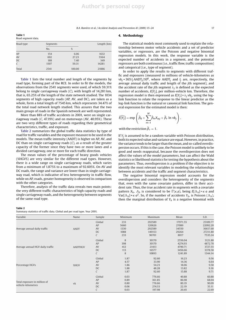
In Spain, the internal transport of goods, as measured in ton-kmand carried out by different modes, of transportation, has expe-rienced a considerable increase since 1950 (MFOM, 2005). Thisgrowth has not been the same in all modes, with road transporthaving experienced the greatest increase in the period. The shareof road transport increased from 24.21% in 1950 to 84.62% in 2006,while rail transport decreased from 35.74% to 2.66% (Fig. 1). Theincrease in mobility and road freight traffic (in millions of vehicle-kilometres) has highlighted the need for a quantitative evaluationof its influence on safety and the environment (Fig. 2). Between1993 and 2005 the total number of accidents on Spanish interurbanroads and those involving at least one HGV, have increased by 19%and 17%, respectively (Fig. 3). On average, in 5.7% of accidents therewas at least one HGV involved, 86% of which happened on interur-ban roads: 57% on single carriageway roads and 37% on high capac-ity roads and the remaining 5% on minor roads (data from 2005).

∗ Corresponding author. Tel.: +34 913363014; fax: +34 913363014.E-mail addresses: [email protected], barenas [email protected]

(B.A. Ramírez), [email protected], [email protected] (F.A. Izquierdo),[email protected] (C.G. Fernández), [email protected] (A.G. Méndez).

1 Tel.: +34 913363014; fax: +34 913365305.2 Tel.: +34 913363149; fax: +34 913363014.

In the 2005–2008 Strategic Road Safety Plan (PESV05-08), theGeneral Directorate of Traffic set the general aim of improving roadsafety in Spain, and proposed reducing the number of deaths by 40%by 2008, from the 2003 level as well as reducing the seriousnessof accidents. Taking account of the country’s accident pattern, thePESV05-08 set as one of its strategic objectives to reduce the totalnumber of HGVs involved in accidents with victims on main roadsand single carriageway roads.

The increasing trend in freight road traffic, mobility and acci-dents, are the motivations for this study, which is related to roadtransport and the evaluation of specific countermeasures devotedto increasing the safety performance of Spanish roads.

Bearing in mind the increasing trend in goods traffic, theincrease in mobility on the Spanish roads and the greater sever-ity of accidents involving HGVs on interurban roads, the interestin this study is evident. In this work, we propose a methodologyto analyze the influence of HGVs on traffic accidents, using generallinear models.

This paper first addresses the identification of factors related tovehicle flow and composition (i.e., cars and HGV vehicles), in roadaccidents on road sections of the state network (RCE), by using neg-ative binomial count regression models to predict accidents. Then,the paper addresses the analysis and evaluation of hypotheticalHGV reduction scenarios based on the decrease of HGVs annualaverage daily traffic on road sections of two representative freighttransportation corridors.

0001-4575/$ – see front matter © 2008 Elsevier Ltd. All rights reserved.doi:10.1016/j.aap.2008.07.016


16 B.A. Ramírez et al. / Accident Analysis and Prevention 41 (2009) 15–24

Fig. 1. Freight modal shift transport (in % of ton-km (million)) 1950–2006.

The format of the paper is as follows: Section 2 briefly presentsthe literature review. Section 3 describes the data used in the work.In Section 4, some details of the model, the goodness of fit mea-sures, and some ideas about the interpretation of the coefficientsare given. Section 5 analyses the fitted model. In Section 6 the appli-cations to the two freight transportation corridors are detailed,along with the study of hypothetical traffic scenarios in these twocorridors. Section 7 summarizes main conclusions, and finally anAppendix A is included with the acronyms used in the paper.

Fig. 2. Annual mobility (total and HGV) on Spanish RCE roads 1993–2005.

Fig. 3. Accidents figures on Spanish roads 1993–2005.

2. Literature review

Poisson and negative binomial regression models have beenapplied to estimate accident frequency and accident rates, withnon-behavioural factors like road features, traffic characteristics,and weather or environmental conditions. From an empirical stand-point, the relation between crash frequency and vehicle-kilometrestravelled and environmental conditions can be found in Jovanis andChang (1986), with environmental factors in Shankar et al. (1995),with average hourly traffic volume per lane, average occupancy,lane occupation, average speed, and its standard deviation, cur-vature, and exposure in Garber and Wu (2001); and with roadgeometry and traffic characteristics in Vogt and Bared (1998),Miaou and Lum (1993), and Abdel-Aty and Radwan (2000).

Other studies have attempted to relate accident rates with trafficcharacteristics and the frequency of intersections (Ivan and O’Mara,1997); hourly traffic volume (Martin, 2002); level of service, lightconditions and the site accident characteristics (Ivan et al., 1999);with weather and light (Fridstrøm et al., 1995); and with the hourlytraffic flow of cars and lorries (Hiselius, 2004).

Both approaches (Poisson and negative binomial regression)are considered appropriate from a statistical viewpoint becauseof the distribution of crash counts, but within this methodolog-ical framework, the negative binomial regression is preferred ifoverdispersion is observed, as is common in traffic accident data.

Few studies have studied the effect of heterogeneous flows, andparticularly the effect that the presence of HGVs in the traffic flowhas on accidents. The study most closely related to this paper is thatby Hiselius (2004). In addition, few studies have used predictionmodels as tools for simulating and analysing new scenarios createdby variations in traffic conditions. Precisely, in this work the acci-dent prediction model was used to simulate and evaluate freighttransport corridors under specific traffic conditions that includethe reduction in the number of HGVs.

3. Data

This work used accident data from the DGT database (Accidentsdatabase, 2001) which covers police-reported accidents with atleast one person injured during 2001 in segments belonging to dif-ferent roads categories of the RCE network, i.e., toll motorways (AP),dual carriageways (AV), two undivided dual carriageways (DC), andsingle carriageway roads (C).

The general criterion for including an accident in the databaseis that it is accident with victims and did not depend on the roadtype. Following this criterion, it may be thought that all accidentswhere there was a fatality or serious injuries are reported. How-ever, in accidents with minor injuries there may be a certain lossof information, but this has still not been objectively evaluated,and is under discussion by several researchers (Lardelli-Claret etal., 2003). Segments refer here to bi-directional stretches, and canbe considered to have homogeneous traffic conditions and constanttraffic flow.

Traffic data are available for the whole RCE network in termsof aggregate estimates of average annual daily traffic (AADT), andaverage annual daily traffic per vehicle type, i.e., average annualHGV daily traffic (AADTHGV) in the traffic map produced by theMinistry of Public Works (Traffic Map, 2001). Traffic flow is countedas the number of vehicles through a fixed section in both directions,and the counts are performed using both portable counting instru-ments and permanent inductive loop detectors. Only 2541 roadsegments were extracted out of a total of 3085 from the 2001 trafficmap, after selection criteria based on the complete information fortraffic flow and reported accidents.


B.A. Ramírez et al. / Accident Analysis and Prevention 41 (2009) 15–24 17

Table 1Road segment data.

Road type Segments Length (km)

No. %

AP 154 6.06 1632AV 692 27.23 5564DC 188 7.40 349C 1507 59.31 14281

Total 2541 100.00 21886

Table 1 lists the total number and length of the segments byroad type, forming part of the RCE. In order to fit the models, theobservations from the 2541 segments were used, of which 59.31%belong to single carriageway roads (C), with length of 14,281 km,that is, 65.25% of the length of the state network studied. The 1034segments of high capacity roads (AP, AV, and DC), are taken as awhole, form a total length of 7545 km, which represents 34.47% ofthe total road network length studied. This assures that the twomain groups of roads in the Spanish network are well represented.

More than 88% of traffic accidents in 2001, were on single car-riageway roads (C, 47.19%) and on motorways (AV, 40.95%). Theseare two very different types of roads regarding their geometricalcharacteristics, traffic, and exposure.

Table 2 summarizes the global traffic data statistics by type ofroad for traffic variables and the exposure measure to be used in themodels. The mean traffic intensity (AADT) is higher on AP, AV, andDC than on single carriageway roads (C), as a result of the greatercapacity of the former since they have two or more lanes and adivided carriageway, one or more for each traffic direction.

The mean values of the percentage of heavy goods vehicles(%HGVS) are very similar for the different road types. However,there is a wide range on single carriageway roads, which variesfrom a minimum of 1.875% to a maximum of 92.605%. On AV andDC roads, the range and variance are lower than in single carriage-way road, which is indicative of less heterogeneity in traffic flow,while on AP, roads, greater homogeneity is observed in comparisonwith the other categories.

Therefore, analysis of the traffic data reveals two main points:the very different traffic characteristics of high capacity roads andsingle carriageway roads, and the heterogeneity between segmentsof the same road type.

4. Methodology

The statistical models most commonly used to explain the rela-tionship between motor vehicle accidents and a set of predictorvariables, or regressors, are the Poisson and negative binomialregression models. In this work, the response variable is theexpected number of accidents in a segment, and the potentialregressors are both continuous (i.e., traffic flow, traffic composition)and categorical (i.e., type of segment).

In order to apply the results to segments with different traf-fic and exposures (measured in millions of vehicle-kilometres asvkj = 365 lj AADTj/106, where AADTj and lj are, respectively, theaverage annual daily traffic and length of the jth segment), andthe accident rate of the jth segment �j is defined as the expectednumber of accidents, E[Yj], per million-vehicle km. Therefore, theregression model is then expressed as E[Yj] = �j vkj, using the log-link function to relate the response to the linear predictor as thelog-link function is the natural or canonical link function. The gen-eral expression for the estimated model is then:

E[Yj] = exp

(ˆ 0 +

M∑m=1

ˆ mXmj + ˆ v ln vkj

),

with the restriction ˆ � = 1.

If Yj is assumed to be a random variable with Poisson distribution,both its expected value and variance are equal. However, in practice,the variance tends to be larger than the mean, and so-called overdis-persion occurs. If this is the case, the Poisson model is unlikely to begood and needs reappraisal, because the overdispersion does notaffect the values of the model parameters, but can affect the Waldstatistics or likelihood statistics for testing the hypothesis about theparameters. Thus, overdispersion is a problem if the objective is toidentify the most relevant variables in modeling the relationshipsbetween accidents and the traffic and segment characteristics.

The negative binomial regression model accounts for theoverdispersion and considers the heterogeneity of the segmentsthat, even with the same covariate pattern, differ in their acci-dent rate. Thus, the true accident rate in segments with a covariatepattern Xh, �h is considered to be �(�,a), being E[�h] = �·a andVar[�h] = �·a2. So, if the number of accidents Yh, is Poisson (�h),then the marginal distribution of Yh is a negative binomial with

Table 2Summary statistics of traffic data. Global and per road type. Year 2001.

Variable Name Sample Minimum Maximum Mean S.D.

Average annual daily traffic AADT

Global 233 292589 17971.55 25109.77AP 5660 120626 27089 22092.20AV 1330 292589 34550 36617.60DC 1088 149153 29264 27211.80C 233 96701 8017 7535.24

Average annual HGV daily traffic AADTHGV

Global 8 30170 2556.04 3121.88AP 398 30170 4274.93 4872.78AV 412 21413 4790.71 3727.55DC 113 16577 3456.66 3378.58C 8 10893 1241.89 1344.14

Percentage HGVs %HGV

Global 1.87 92.60 16.23 9.56AP 4.57 33.90 14.36 6.64AV 1.86 54.23 18.06 9.58DC 1.88 48.28 13.82 9.16C 1.87 92.60 15.88 9.71

Total exposure in million ofvehicle-kilometres

vk

Global 0.03 776.66 40.88 60.88AP 0.89 361.85 86.98 68.04AV 0.80 776.66 80.19 90.09DC 0.06 274.53 22.19 35.11C 0.03 197.98 20.45 22.69



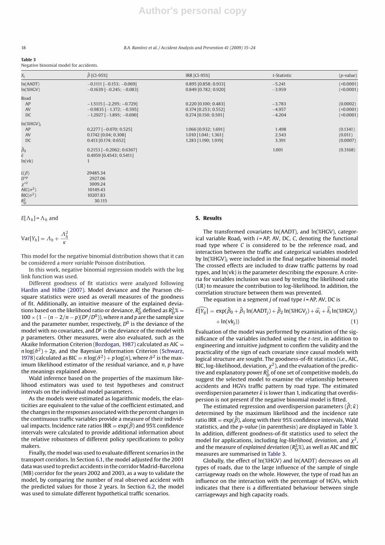
Table 3Negative binomial model for accidents.

Xiˆ [CI-95%] IRR [CI-95%] t-Statistic (p-value)

ln(AADT) −0.1111 [−0.153; −0.069] 0.895 [0.858; 0.933] −5.241 (<0.0001)ln(%HGV) −0.1639 [−0.245; −0.083] 0.849 [0.782; 0.920] −3.959 (<0.0001)

RoadAP −1.5115 [−2.295; −0.729] 0.220 [0.100; 0.483] −3.783 (0.0002)AV −0.9835 [−1.372; −0.595] 0.374 [0.253; 0.552] −4.957 (<0.0001)DC −1.2927 [−1.895; −0.690] 0.274 [0.150; 0.501] −4.204 (<0.0001)

ln(%HGV)iAP 0.2277 [−0.070; 0.525] 1.066 [0.932; 1.691] 1.498 (0.1341)AV 0.1742 [0.04; 0.308] 1.010 [1.041; 1.361] 2.543 (0.011)DC 0.413 [0.174; 0.652] 1.283 [1.190; 1.919] 3.391 (0.0007)

ˆ 0 0.2153 [−0.2062; 0.6367] 1.001 (0.3168)� 0.4959 [0.4543; 0.5411]ln(vk) 1

L(ˇ) 29485.34D*p 2927.06�*2 3009.24AIC(2) 10149.43BIC(2) 10207.83R2

D 30.115

E[�h] = �h and

Var[Yh] = �h + �2h

�

This model for the negative binomial distribution shows that it canbe considered a more variable Poisson distribution.

In this work, negative binomial regression models with the loglink function was used.

Different goodness of fit statistics were analyzed followingHardin and Hilbe (2007). Model deviance and the Pearson chi-square statistics were used as overall measures of the goodnessof fit. Additionally, an intuitive measure of the explained devia-tions based on the likelihood ratio or deviance, R2

D defined as R2D% =

100 × (1 − (n − 2/n − p)(Dp/D0)), where n and p are the sample sizeand the parameter number, respectively, D0 is the deviance of themodel with no covariates, and Dp is the deviance of the model withp parameters. Other measures, were also evaluated, such as theAkaike Information Criterion (Bozdogan, 1987) calculated as AIC =n log(2) + 2p, and the Bayesian Information Criterion (Schwarz,1978) calculated as BIC = n log(2) + p log(n), where 2 is the max-imum likelihood estimator of the residual variance, and n, p havethe meanings explained above.

Wald inference based on the properties of the maximum like-lihood estimators was used to test hypotheses and constructintervals on the individual model parameters.

As the models were estimated as logarithmic models, the elas-ticities are equivalent to the value of the coefficient estimated, andthe changes in the responses associated with the percent changes inthe continuous traffic variables provide a measure of their individ-ual impacts. Incidence rate ratios IRR = exp( ˆ ) and 95% confidenceintervals were calculated to provide additional information aboutthe relative robustness of different policy specifications to policymakers.

Finally, the model was used to evaluate different scenarios in thetransport corridors. In Section 6.1, the model adjusted for the 2001data was used to predict accidents in the corridor Madrid-Barcelona(MB) corridor for the years 2002 and 2003, as a way to validate themodel, by comparing the number of real observed accident withthe predicted values for those 2 years. In Section 6.2, the modelwas used to simulate different hypothetical traffic scenarios.

5. Results

The transformed covariates ln(AADT), and ln(%HGV), categor-ical variable Roadi with i = AP, AV, DC, C, denoting the functionalroad type where C is considered to be the reference road, andinteraction between the traffic and categorical variables modeledby ln(%HGV)i were included in the final negative binomial model.The crossed effects are included to draw traffic patterns by roadtypes, and ln(vk) is the parameter describing the exposure. A crite-ria for variables inclusion was used by testing the likelihood ratio(LR) to measure the contribution to log-likelihood. In addition, thecorrelation structure between them was prevented.

The equation in a segment j of road type i = AP, AV, DC is

E[Yij] = exp( ˆ 0 + ˆ 1 ln(AADTj) + ˆ 2 ln(%HGVj) + i + ıi ln(%HGVj)

+ ln(vkj)) (1)

Evaluation of the model was performed by examination of the sig-nificance of the variables included using the t-test, in addition toengineering and intuitive judgment to confirm the validity and thepracticality of the sign of each covariate since causal models withlogical structure are sought. The goodness-of-fit statistics (i.e., AIC,BIC, log-likelihood, deviation, �2), and the evaluation of the predic-tive and explanatory power R2

D of one set of competitive models, dosuggest the selected model to examine the relationship betweenaccidents and HGVs traffic pattern by road type. The estimatedoverdispersion parameter � is lower than 1, indicating that overdis-persion is not present if the negative binomial model is fitted.

The estimated regression and overdispersion parameters ( ˆ ; �)determined by the maximum likelihood and the incidence rateratio IRR = exp( ˆ ), along with their 95% confidence intervals, Waldstatistics, and the p-value (in parenthesis) are displayed in Table 3.In addition, different goodness-of-fit statistics used to select themodel for applications, including log-likelihood, deviation, and �2,and the measure of explained deviation (R2

D%), as well as AIC and BICmeasures are summarised in Table 3.

Globally, the effect of ln(%HGV) and ln(AADT) decreases on alltypes of roads, due to the large influence of the sample of singlecarriageway roads on the whole. However, the type of road has aninfluence on the interaction with the percentage of HGVs, whichindicates that there is a differentiated behaviour between singlecarriageways and high capacity roads.



Table 4Accident rates �h

a by road type.

Global AP AV DC C

�h 0.264 0.104 0.20 0.209 0.290IP(�h) [95%] [0; 1.001] [0; 0.396] [0; 0.567] [0; 0.804] [0; 1.098]�h 0.259 0.106 0.162 0.213 0.324Differences (%) 2.13 −1.60 −7.65 −1.92 −10.37

�h: observed accident rate; �h: calculated accident rate by Eqs. (2). �h: safety at a new site. IP (�h): prediction interval of safety at a new site.a Rates are accidents with injured people per 1 million vehicle-kilometres (ATi

/vki).

The crossed effect ln(%HGV) and Roadi, modelled by ln(%HGVi),has the opposite sign from that found between ln(%HGV) andresponse, reversing the fundamental relationship in AP, AV, and DCroad types, and determining a different behaviour of C roads withinthe Spanish network.

The coefficients of the road type variable (Roadi) reveal signifi-cant differences (according to Pearson’s �2) between high capacityand single carriageway roads. The signs associated with high capac-ity roads are negative and show that the predicted number ofaccidents on these roads is lower than for single carriageway roads.The hypothesis test performed for the coefficients corresponding tohigh capacity roads reveals that there are not significant differencesbetween them. Likewise, the hypotheses test on the coefficientscorresponding to the interaction ln(%HGV)-Roadi, particularized toAP and AV does not reject the null hypothesis.

The expressions of the accident rates by road types (i) and seg-ment (j) are calculated to be

�ij =E[Yij]vkj

�APj= 0.2736(AADTj)

−0.1111(%HGVj)0.0638

�AVj= 0.4368(AADTj)

−0.1111(%HGVj)0.0103

�DCj= 0.3405(AADTj)

−0.1111(%HGVj)0.2491

�Cj= 1.2402(AADTj)

−0.1111(%HGVj)−0.1639

(2)

5.1. Average rates

For all of the segments included in this work, Eqs. (2) wereapplied in order to calculate point estimates of the accident rate.In addition, prediction intervals were obtained according to theapproach given by McCullagh and Nelder (1989) and Wood (2005).

To generalize the results, point estimates of the accident rates�h, and the prediction interval for the safety, �h, of a new segmentof each type of road are presented in Table 4. The calculations wereperformed assuming that the covariate values of the new segmentare the mean values of the regressors in the respective type of road.Also, in Table 4, the average of the observed accident rates �h ispresented.

The calculated value for C roads turned out to be 0.290, which isabout 3 times the calculated value for AP roads, twice that for theAV roads, and 1.5 times that corresponding to DC roads.

The calculated values show large differences between C roadsand the other types AP, AV, which are usually classified in the sameroad class. In fact, the Ministry of Public Works (MFOM) includesAP, DC and AV roads in one homogeneous group denoted by thehigh capacity roads category, which are generally considered asinherently safer routes. However, the single carriageway roads (C)include intersections and railroad grade crossing, and the trafficflow in both directions is not separated. Therefore a higher crashrisk was expected than for the unfied class, and this was observed.

When the analysis was performed by road type, the greater het-erogeneity on single carriageway roads allowed establishing the

hypothesis of differential behaviour and a higher accident rate thanother road types, which is reflected in the previous figures.

For DC roads, an intermediate behaviour between AP, AV and C,can be seen, which agress with what was expected, since althoughthere is more than one lane in both directions, as with AP and AVroads, there is no traffic flow separation as in type C roads.

These results agree with the observed data. The number of acci-dents per vehicle-km produced in the Spanish RCE is larger for thisclass of roads than motorways like AP or AV.

From annual mobility and accident figures on Spanish RCE roadsfor the 1990–2004 period an average value for the accident rate of0.143 is obtained on high capacity roads and 0.328 on single car-riageway roads, which confirms the values found using the adjustedmodel.

5.2. Elasticities and incidence rate ratios

One of the key uses of the coefficients is the evaluation of therelative elasticities of the covariates in the accident rate. Since loga-rithmic models provide an straightforward way to quantify relativeeffects by means of estimated coefficients, their confidence inter-vals can also be used to bound inferences.

In this case, ln(AADT) is more relevant when explaining theresponse of AP and AV roads, while ln(%HGV) is on DC and C roads,although all parameters can be considered inelastic.

For instance, a variation in AADT could have the same impactregardless of road type, because the terms for the interactionbetween AADT and road type are not statiscally significant.

Different behaviour could be expected for the variation %HGVbetween high capacity roads (AP, AV, and DC) and single carriage-way roads, denoted by C. A 10% variation in %HGV, induces a 0.6%increase in AP rates, 0.1% in AV, or 2.5% in DC, but causes a decreaseof 1.6% in C roads.

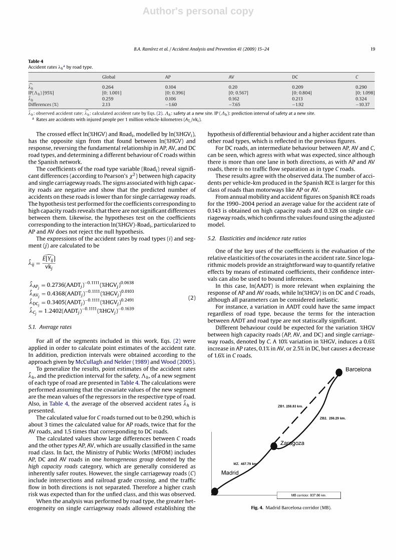
Fig. 4. Madrid Barcelona corridor (MB).



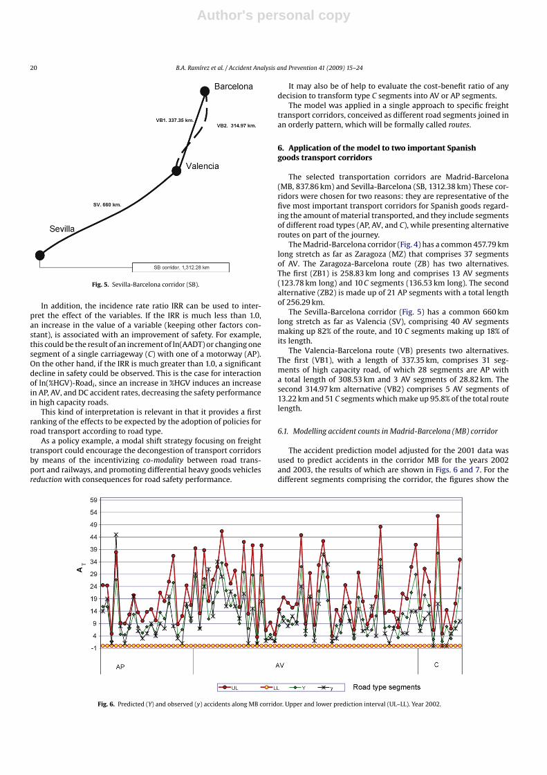
Fig. 5. Sevilla-Barcelona corridor (SB).

In addition, the incidence rate ratio IRR can be used to inter-pret the effect of the variables. If the IRR is much less than 1.0,an increase in the value of a variable (keeping other factors con-stant), is associated with an improvement of safety. For example,this could be the result of an increment of ln(AADT) or changing onesegment of a single carriageway (C) with one of a motorway (AP).On the other hand, if the IRR is much greater than 1.0, a significantdecline in safety could be observed. This is the case for interactionof ln(%HGV)-Roadi, since an increase in %HGV induces an increasein AP, AV, and DC accident rates, decreasing the safety performancein high capacity roads.

This kind of interpretation is relevant in that it provides a firstranking of the effects to be expected by the adoption of policies forroad transport according to road type.

As a policy example, a modal shift strategy focusing on freighttransport could encourage the decongestion of transport corridorsby means of the incentivizing co-modality between road trans-port and railways, and promoting differential heavy goods vehiclesreduction with consequences for road safety performance.

It may also be of help to evaluate the cost-benefit ratio of anydecision to transform type C segments into AV or AP segments.

The model was applied in a single approach to specific freighttransport corridors, conceived as different road segments joined inan orderly pattern, which will be formally called routes.

6. Application of the model to two important Spanishgoods transport corridors

The selected transportation corridors are Madrid-Barcelona(MB, 837.86 km) and Sevilla-Barcelona (SB, 1312.38 km) These cor-ridors were chosen for two reasons: they are representative of thefive most important transport corridors for Spanish goods regard-ing the amount of material transported, and they include segmentsof different road types (AP, AV, and C), while presenting alternativeroutes on part of the journey.

The Madrid-Barcelona corridor (Fig. 4) has a common 457.79 kmlong stretch as far as Zaragoza (MZ) that comprises 37 segmentsof AV. The Zaragoza-Barcelona route (ZB) has two alternatives.The first (ZB1) is 258.83 km long and comprises 13 AV segments(123.78 km long) and 10 C segments (136.53 km long). The secondalternative (ZB2) is made up of 21 AP segments with a total lengthof 256.29 km.

The Sevilla-Barcelona corridor (Fig. 5) has a common 660 kmlong stretch as far as Valencia (SV), comprising 40 AV segmentsmaking up 82% of the route, and 10 C segments making up 18% ofits length.

The Valencia-Barcelona route (VB) presents two alternatives.The first (VB1), with a length of 337.35 km, comprises 31 seg-ments of high capacity road, of which 28 segments are AP witha total length of 308.53 km and 3 AV segments of 28.82 km. Thesecond 314.97 km alternative (VB2) comprises 5 AV segments of13.22 km and 51 C segments which make up 95.8% of the total routelength.

6.1. Modelling accident counts in Madrid-Barcelona (MB) corridor

The accident prediction model adjusted for the 2001 data wasused to predict accidents in the corridor MB for the years 2002and 2003, the results of which are shown in Figs. 6 and 7. For thedifferent segments comprising the corridor, the figures show the

Fig. 6. Predicted (Y) and observed (y) accidents along MB corridor. Upper and lower prediction interval (UL–LL). Year 2002.



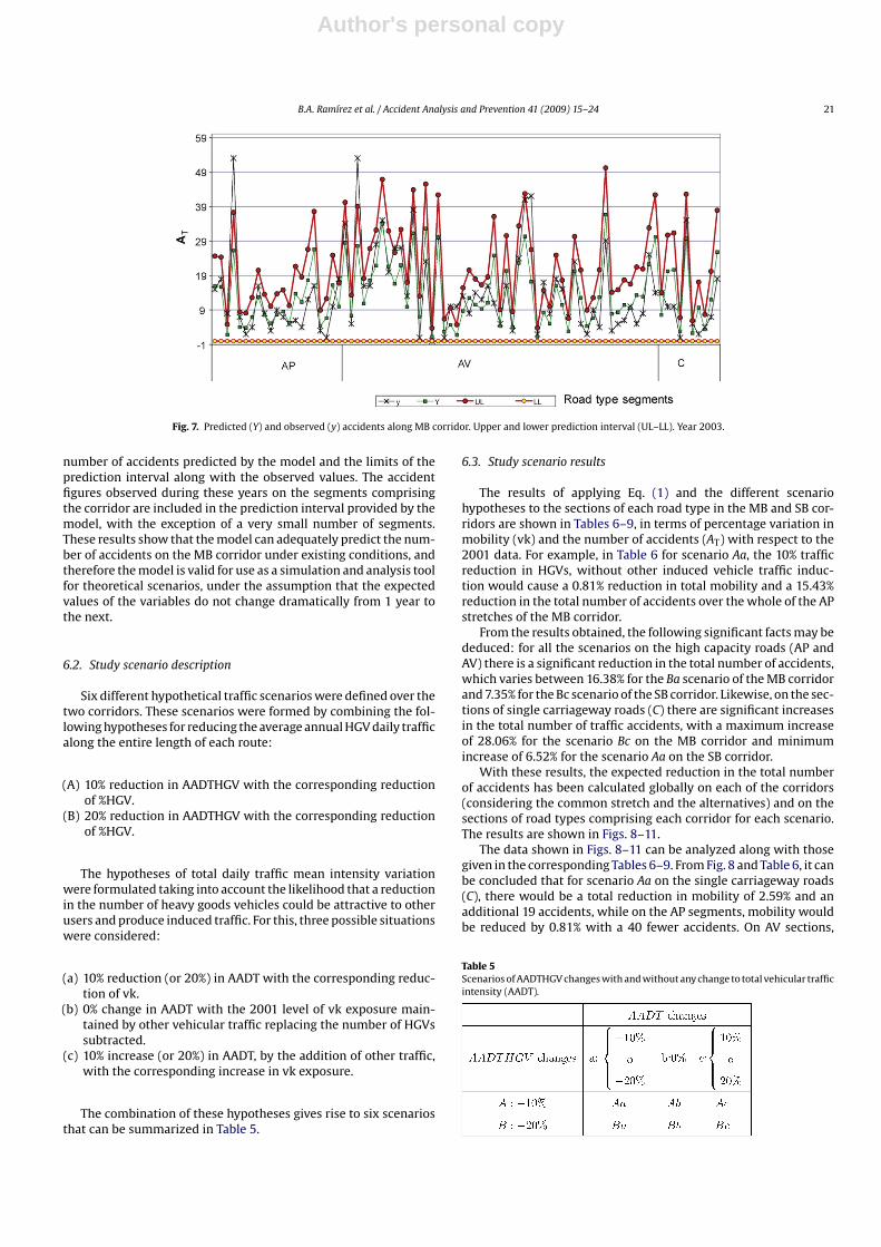
Fig. 7. Predicted (Y) and observed (y) accidents along MB corridor. Upper and lower prediction interval (UL–LL). Year 2003.

number of accidents predicted by the model and the limits of theprediction interval along with the observed values. The accidentfigures observed during these years on the segments comprisingthe corridor are included in the prediction interval provided by themodel, with the exception of a very small number of segments.These results show that the model can adequately predict the num-ber of accidents on the MB corridor under existing conditions, andtherefore the model is valid for use as a simulation and analysis toolfor theoretical scenarios, under the assumption that the expectedvalues of the variables do not change dramatically from 1 year tothe next.

6.2. Study scenario description

Six different hypothetical traffic scenarios were defined over thetwo corridors. These scenarios were formed by combining the fol-lowing hypotheses for reducing the average annual HGV daily trafficalong the entire length of each route:

(A) 10% reduction in AADTHGV with the corresponding reductionof %HGV.

(B) 20% reduction in AADTHGV with the corresponding reductionof %HGV.

The hypotheses of total daily traffic mean intensity variationwere formulated taking into account the likelihood that a reductionin the number of heavy goods vehicles could be attractive to otherusers and produce induced traffic. For this, three possible situationswere considered:

(a) 10% reduction (or 20%) in AADT with the corresponding reduc-tion of vk.

(b) 0% change in AADT with the 2001 level of vk exposure main-tained by other vehicular traffic replacing the number of HGVssubtracted.

(c) 10% increase (or 20%) in AADT, by the addition of other traffic,with the corresponding increase in vk exposure.

The combination of these hypotheses gives rise to six scenariosthat can be summarized in Table 5.

6.3. Study scenario results

The results of applying Eq. (1) and the different scenariohypotheses to the sections of each road type in the MB and SB cor-ridors are shown in Tables 6–9, in terms of percentage variation inmobility (vk) and the number of accidents (AT) with respect to the2001 data. For example, in Table 6 for scenario Aa, the 10% trafficreduction in HGVs, without other induced vehicle traffic induc-tion would cause a 0.81% reduction in total mobility and a 15.43%reduction in the total number of accidents over the whole of the APstretches of the MB corridor.

From the results obtained, the following significant facts may bededuced: for all the scenarios on the high capacity roads (AP andAV) there is a significant reduction in the total number of accidents,which varies between 16.38% for the Ba scenario of the MB corridorand 7.35% for the Bc scenario of the SB corridor. Likewise, on the sec-tions of single carriageway roads (C) there are significant increasesin the total number of traffic accidents, with a maximum increaseof 28.06% for the scenario Bc on the MB corridor and minimumincrease of 6.52% for the scenario Aa on the SB corridor.

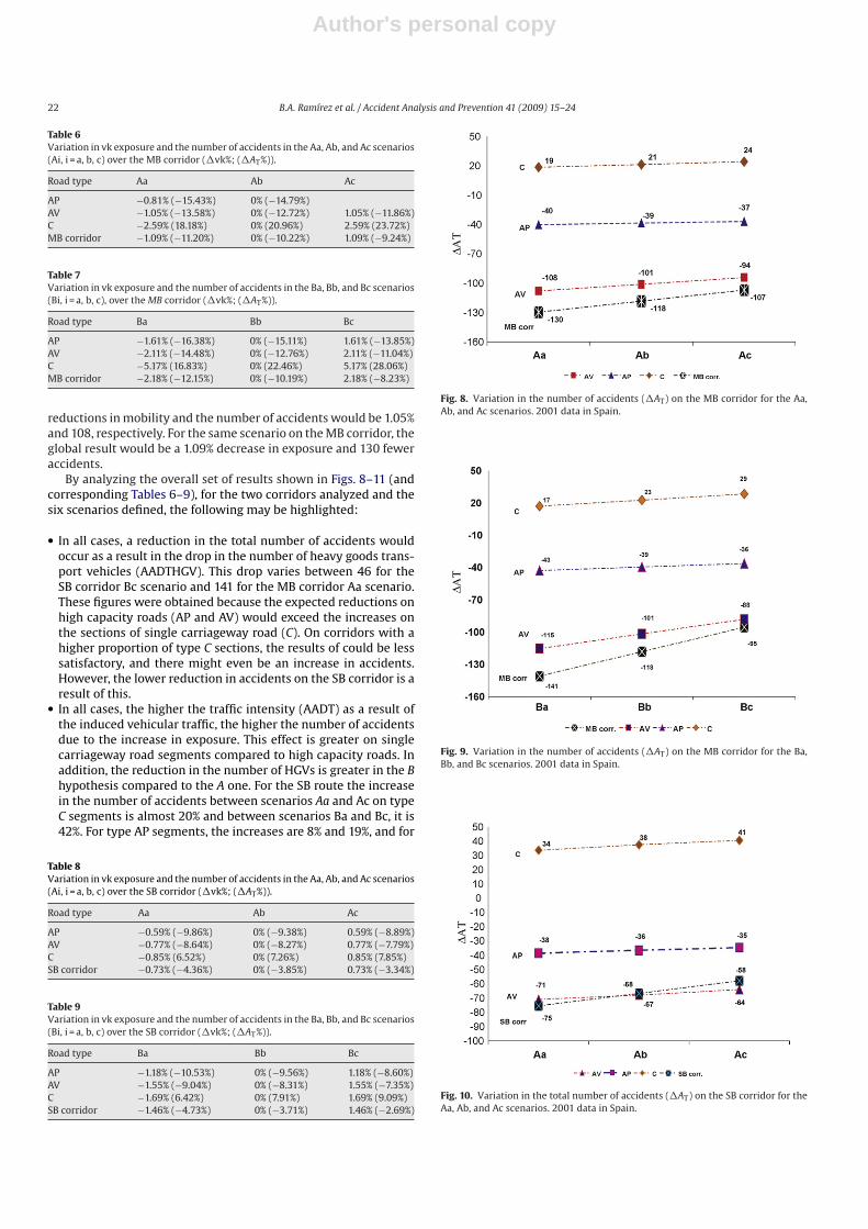
With these results, the expected reduction in the total numberof accidents has been calculated globally on each of the corridors(considering the common stretch and the alternatives) and on thesections of road types comprising each corridor for each scenario.The results are shown in Figs. 8–11.

The data shown in Figs. 8–11 can be analyzed along with thosegiven in the corresponding Tables 6–9. From Fig. 8 and Table 6, it canbe concluded that for scenario Aa on the single carriageway roads(C), there would be a total reduction in mobility of 2.59% and anadditional 19 accidents, while on the AP segments, mobility wouldbe reduced by 0.81% with a 40 fewer accidents. On AV sections,

Table 5Scenarios of AADTHGV changes with and without any change to total vehicular trafficintensity (AADT).



Table 6Variation in vk exposure and the number of accidents in the Aa, Ab, and Ac scenarios(Ai, i = a, b, c) over the MB corridor (vk%; (AT%)).

Road type Aa Ab Ac

AP −0.81% (−15.43%) 0% (−14.79%)AV −1.05% (−13.58%) 0% (−12.72%) 1.05% (−11.86%)C −2.59% (18.18%) 0% (20.96%) 2.59% (23.72%)MB corridor −1.09% (−11.20%) 0% (−10.22%) 1.09% (−9.24%)

Table 7Variation in vk exposure and the number of accidents in the Ba, Bb, and Bc scenarios(Bi, i = a, b, c), over the MB corridor (vk%; (AT%)).

Road type Ba Bb Bc

AP −1.61% (−16.38%) 0% (−15.11%) 1.61% (−13.85%)AV −2.11% (−14.48%) 0% (−12.76%) 2.11% (−11.04%)C −5.17% (16.83%) 0% (22.46%) 5.17% (28.06%)MB corridor −2.18% (−12.15%) 0% (−10.19%) 2.18% (−8.23%)

reductions in mobility and the number of accidents would be 1.05%and 108, respectively. For the same scenario on the MB corridor, theglobal result would be a 1.09% decrease in exposure and 130 feweraccidents.

By analyzing the overall set of results shown in Figs. 8–11 (andcorresponding Tables 6–9), for the two corridors analyzed and thesix scenarios defined, the following may be highlighted:

• In all cases, a reduction in the total number of accidents wouldoccur as a result in the drop in the number of heavy goods trans-port vehicles (AADTHGV). This drop varies between 46 for theSB corridor Bc scenario and 141 for the MB corridor Aa scenario.These figures were obtained because the expected reductions onhigh capacity roads (AP and AV) would exceed the increases onthe sections of single carriageway road (C). On corridors with ahigher proportion of type C sections, the results of could be lesssatisfactory, and there might even be an increase in accidents.However, the lower reduction in accidents on the SB corridor is aresult of this.

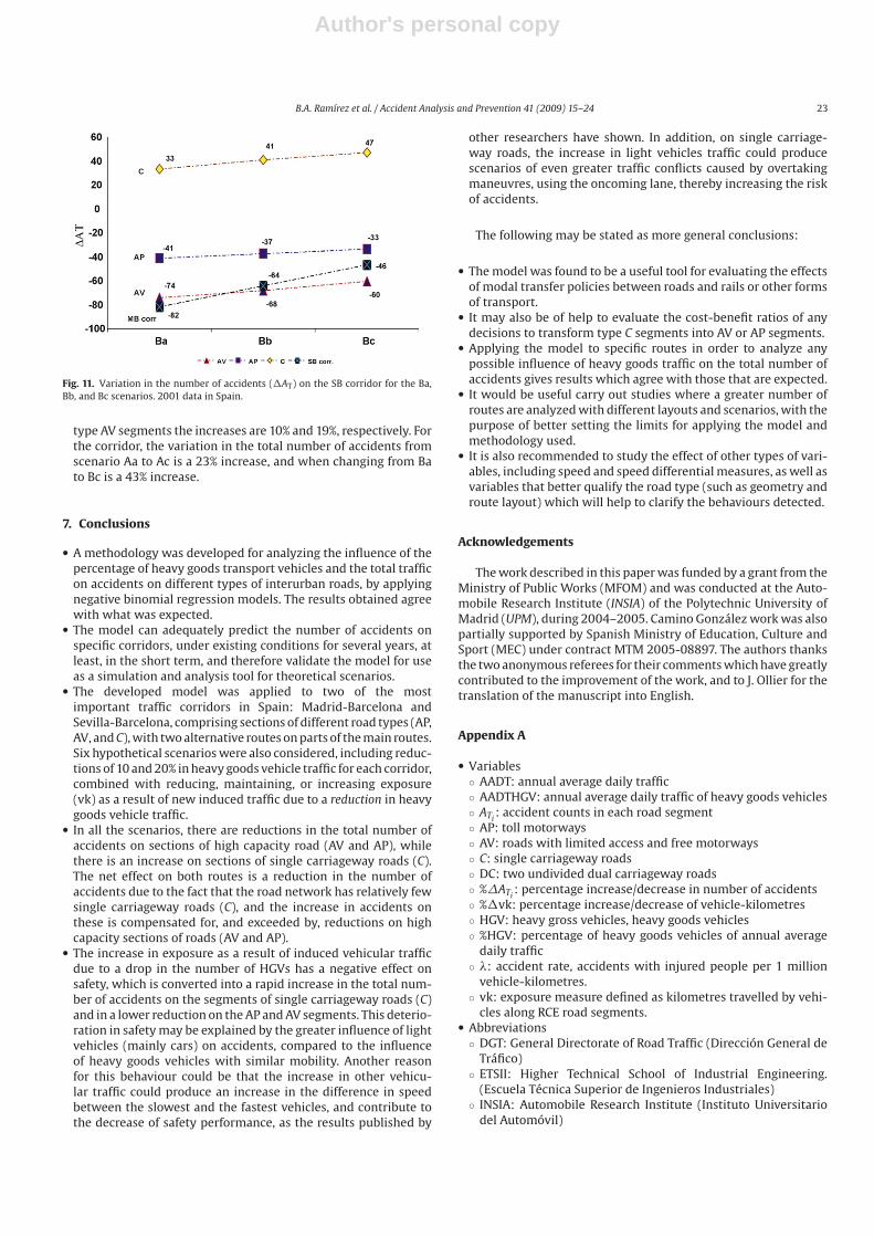
• In all cases, the higher the traffic intensity (AADT) as a result ofthe induced vehicular traffic, the higher the number of accidentsdue to the increase in exposure. This effect is greater on singlecarriageway road segments compared to high capacity roads. Inaddition, the reduction in the number of HGVs is greater in the Bhypothesis compared to the A one. For the SB route the increasein the number of accidents between scenarios Aa and Ac on typeC segments is almost 20% and between scenarios Ba and Bc, it is42%. For type AP segments, the increases are 8% and 19%, and for

Table 8Variation in vk exposure and the number of accidents in the Aa, Ab, and Ac scenarios(Ai, i = a, b, c) over the SB corridor (vk%; (AT%)).

Road type Aa Ab Ac

AP −0.59% (−9.86%) 0% (−9.38%) 0.59% (−8.89%)AV −0.77% (−8.64%) 0% (−8.27%) 0.77% (−7.79%)C −0.85% (6.52%) 0% (7.26%) 0.85% (7.85%)SB corridor −0.73% (−4.36%) 0% (−3.85%) 0.73% (−3.34%)

Table 9Variation in vk exposure and the number of accidents in the Ba, Bb, and Bc scenarios(Bi, i = a, b, c) over the SB corridor (vk%; (AT%)).

Road type Ba Bb Bc

AP −1.18% (−10.53%) 0% (−9.56%) 1.18% (−8.60%)AV −1.55% (−9.04%) 0% (−8.31%) 1.55% (−7.35%)C −1.69% (6.42%) 0% (7.91%) 1.69% (9.09%)SB corridor −1.46% (−4.73%) 0% (−3.71%) 1.46% (−2.69%)

Fig. 8. Variation in the number of accidents (AT) on the MB corridor for the Aa,Ab, and Ac scenarios. 2001 data in Spain.

Fig. 9. Variation in the number of accidents (AT) on the MB corridor for the Ba,Bb, and Bc scenarios. 2001 data in Spain.

Fig. 10. Variation in the total number of accidents (AT) on the SB corridor for theAa, Ab, and Ac scenarios. 2001 data in Spain.



Fig. 11. Variation in the number of accidents (AT) on the SB corridor for the Ba,Bb, and Bc scenarios. 2001 data in Spain.

type AV segments the increases are 10% and 19%, respectively. Forthe corridor, the variation in the total number of accidents fromscenario Aa to Ac is a 23% increase, and when changing from Bato Bc is a 43% increase.

7. Conclusions

• A methodology was developed for analyzing the influence of thepercentage of heavy goods transport vehicles and the total trafficon accidents on different types of interurban roads, by applyingnegative binomial regression models. The results obtained agreewith what was expected.

• The model can adequately predict the number of accidents onspecific corridors, under existing conditions for several years, atleast, in the short term, and therefore validate the model for useas a simulation and analysis tool for theoretical scenarios.

• The developed model was applied to two of the mostimportant traffic corridors in Spain: Madrid-Barcelona andSevilla-Barcelona, comprising sections of different road types (AP,AV, and C), with two alternative routes on parts of the main routes.Six hypothetical scenarios were also considered, including reduc-tions of 10 and 20% in heavy goods vehicle traffic for each corridor,combined with reducing, maintaining, or increasing exposure(vk) as a result of new induced traffic due to a reduction in heavygoods vehicle traffic.

• In all the scenarios, there are reductions in the total number ofaccidents on sections of high capacity road (AV and AP), whilethere is an increase on sections of single carriageway roads (C).The net effect on both routes is a reduction in the number ofaccidents due to the fact that the road network has relatively fewsingle carriageway roads (C), and the increase in accidents onthese is compensated for, and exceeded by, reductions on highcapacity sections of roads (AV and AP).

• The increase in exposure as a result of induced vehicular trafficdue to a drop in the number of HGVs has a negative effect onsafety, which is converted into a rapid increase in the total num-ber of accidents on the segments of single carriageway roads (C)and in a lower reduction on the AP and AV segments. This deterio-ration in safety may be explained by the greater influence of lightvehicles (mainly cars) on accidents, compared to the influenceof heavy goods vehicles with similar mobility. Another reasonfor this behaviour could be that the increase in other vehicu-lar traffic could produce an increase in the difference in speedbetween the slowest and the fastest vehicles, and contribute tothe decrease of safety performance, as the results published by

other researchers have shown. In addition, on single carriage-way roads, the increase in light vehicles traffic could producescenarios of even greater traffic conflicts caused by overtakingmaneuvres, using the oncoming lane, thereby increasing the riskof accidents.

The following may be stated as more general conclusions:

• The model was found to be a useful tool for evaluating the effectsof modal transfer policies between roads and rails or other formsof transport.

• It may also be of help to evaluate the cost-benefit ratios of anydecisions to transform type C segments into AV or AP segments.

• Applying the model to specific routes in order to analyze anypossible influence of heavy goods traffic on the total number ofaccidents gives results which agree with those that are expected.

• It would be useful carry out studies where a greater number ofroutes are analyzed with different layouts and scenarios, with thepurpose of better setting the limits for applying the model andmethodology used.

• It is also recommended to study the effect of other types of vari-ables, including speed and speed differential measures, as well asvariables that better qualify the road type (such as geometry androute layout) which will help to clarify the behaviours detected.

Acknowledgements

The work described in this paper was funded by a grant from theMinistry of Public Works (MFOM) and was conducted at the Auto-mobile Research Institute (INSIA) of the Polytechnic University ofMadrid (UPM), during 2004–2005. Camino González work was alsopartially supported by Spanish Ministry of Education, Culture andSport (MEC) under contract MTM 2005-08897. The authors thanksthe two anonymous referees for their comments which have greatlycontributed to the improvement of the work, and to J. Ollier for thetranslation of the manuscript into English.

Appendix A

• Variables◦ AADT: annual average daily traffic◦ AADTHGV: annual average daily traffic of heavy goods vehicles◦ ATi

: accident counts in each road segment◦ AP: toll motorways◦ AV: roads with limited access and free motorways◦ C: single carriageway roads◦ DC: two undivided dual carriageway roads◦ %�ATi

: percentage increase/decrease in number of accidents◦ %vk: percentage increase/decrease of vehicle-kilometres◦ HGV: heavy gross vehicles, heavy goods vehicles◦ %HGV: percentage of heavy goods vehicles of annual average

daily traffic◦ �: accident rate, accidents with injured people per 1 million

vehicle-kilometres.◦ vk: exposure measure defined as kilometres travelled by vehi-

cles along RCE road segments.• Abbreviations

◦ DGT: General Directorate of Road Traffic (Dirección General deTráfico)

◦ ETSII: Higher Technical School of Industrial Engineering.(Escuela Técnica Superior de Ingenieros Industriales)

◦ INSIA: Automobile Research Institute (Instituto Universitariodel Automóvil)



◦ MEC: Ministry of Education, Culture and Sports (Ministerio deEducación, Cultura y Deporte)

◦ MFOM: Ministry of Public Work (Ministerio de Fomento)◦ RCE: Spanish Interurban Road State Network (Red de Carreteras

del Estado)◦ UPM: Polytechnic University of Madrid (Universidad Politéc-

nica de Madrid)◦ PESV05-08: 2005–2008 Strategic Road Safety Plan (Plan

Estratégico de Seguridad Vial, 2005–2008)◦ MB: Madrid-Barcelona corridor◦ MZ: Madrid-Zaragoza route◦ ZB: Zaragoza-Barcelona ruote◦ SB: Sevilla-Barcelona corridor◦ SV: Sevilla-Valencia route◦ VB: Valencia-Barcelona route

References

Abdel-Aty, M.A., Radwan, A.E., 2000. Modeling traffic accident occurrence andinvolvement. Accident Analysis and Prevention 32 (5), 633–642.

Accidents database, 2001. Dirección General de Tráfico, Spain.MFOM, 2005. Los transportes y los servicios postales. Informe anual 2005. Ministerio

de Fomento, Spain.Bozdogan, H., 1987. Model selection and Akaike’s Information Criterion (AIC):

the general theory and its analytical extensions. Psychometrika 52, 345–370.

PESV05-08, 2005. Plan Estratégico de Seguridad Vial 2005-2008. Dirección Generalde Tráfico. Spain.

Fridstrøm, L., Ifver, J., Ingebrigtsen, S., Kulmala, R., Thomsen, L., 1995. Measuring thecontribution of randomness, exposure, weather, and daylight to the variation inroad accident counts. Accident Analysis and Prevention 27 (1), 1–20.

Garber, N., Wu, L., 2001. Stochastic models relating crash probabilities withgeometrics and corresponding traffic characteristics data. Research Report

No. UVACTS-5-15-74. Center for Transportation Studies at the University ofVirginia.

Hardin, J.W., Hilbe, J.M., 2007. Generalized Linear Models and Extensions, 2nd ed.Stata Press.

Hiselius, L.W., 2004. Estimating the relationship between accident frequency andhomogeneous and inhomogeneous traffic flows. Accident Analysis and Preven-tion 36, 985–992.

Ivan, J., O’Mara, P., 1997. Prediction of traffic accident rates using Poisson regression.76th Annual Meeting of the Transportation Research Board. Washington, D.C.Paper No. 970861.

Ivan, J.N., Pasupathy, R.K., Ossenbruggen, P.J., 1999. Differences in causality factorsfor single and multi-vehicle crashes on two-lane roads. Accident Analysis andPrevention 31 (6), 695–704.

Jovanis, P., Chang, H.L., 1986. Modeling the relationship of accidents to miles trav-elled. Transportation Research Board 1068, 42–51.

Lardelli-Claret, P., Luna-Del-Castillo, J., Jiménez-Moleón, J., Rueda-Domínguez, T.,García-Martín, M., Femia-Marzo, P., Bueno-Cavanillas, A., 2003. Association ofmain driver-dependent risk factors with the risk of causing a vehicle collision inSpain, 1990–1999. Annals of Epidemiology 14 (7), 509–517.

Martin, J.L., 2002. Relationship between rate and hourly traffic flow on interurbanmotorways. Accident Analysis and Prevention 34, 619–629.

McCullagh, P., Nelder, J.A., 1989. Generalized Linear Models, 2nd ed. Chapman &Hall/CRC, Florida.

Miaou, S.P., Lum, H., 1993. Modeling vehicle accident and highway geometric designrelationships. Accident Analysis and Prevention 25 (6), 689–709.

Shankar, V., Mannering, F., Barfield, W., 1995. Effect of roadway geometrics and envi-ronmental factors on rural freeway accidents frequencies. Accident Analysis andPrevention 27 (3), 371–389.

Schwarz, G., 1978. Estimating the dimension of a model. The Annals of Statistics 6,461–464.

Traffic Map, 2001. Ministerio de Fomento. Dirección General de Carreteras, Madrid,Spain.

Vogt A., Bared J., 1998. Accident models for two-lane rural segments and inter-sections, Transportation Research Record 1635, Transportation Research Board.Washington. D.C. 18–29.

Wood, G.R., 2005. Confidence and prediction intervals for generalised linear accidentmodels. Accident Analysis and Prevention 37, 267–273.

The influence of heavy goods vehicle traffic on accidents on different types of Spanish interurban...

Documents

Transcript of The influence of heavy goods vehicle traffic on accidents on different types of Spanish interurban...