D S E Working Paper

The Impact of TemperatureChange on Energy Demand:a Dynamic Panel Analisys

Enrica De CianElisa LanziRoberto Roson

Dipartimento Scienze Economiche

Department of Economics

Ca’ Foscari University ofVenice

ISSN: 1827/336X This paper can be downloaded without charge from the Social Science Research Network (SSRN) electronic library at: http://ssrn.com/abstract=986306

No. 04/WP/2006

W o r k i n g P a p e r s D e p a r t m e n t o f E c o n o m i c s

C a ’ F o s c a r i U n i v e r s i t y o f V e n i c e N o . 0 4 / W P / 2 0 0 7

ISSN 1827-3580

The Working Paper Series is availble only on line

(www.dse.unive.it/pubblicazioni) For editorial correspondence, please contact:

wp.dse@unive.it

Department of Economics Ca’ Foscari University of Venice Cannaregio 873, Fondamenta San Giobbe 30121 Venice Italy Fax: ++39 041 2349210

The Impact of Temperature Change on Energy Demand:

a Dynamic Panel Analysis

Enrica De Cian*, Elisa Lanzi* and Roberto Roson**

* S ch o o l o f A d v a n c e d S tu d i e s i n V e n ic e a n d F o n d a z i o n e E N I E n r i c o M a t t e i ** University Ca’ Foscari of Venice and Fondazione ENI Enrico Mattei

First Draft: April 2007

Abstract This paper presents an empirical study of energy demand, in which demand for a series of energy goods (Gas, Oil Products, Coal, Electricity) is expressed as a function of various factors, including temperature. Parameter values are estimated econometrically, using a dynamic panel data approach. Unlike previous studies in this field, the data sample has a global coverage, and special emphasis is given to the dynamic nature of demand, as well as to interactions between income levels and sensitivity to temperature variations. These features make the model results especially valuable in the analysis of climate change impacts. Results are interpreted in terms of derived demand for heating and cooling. Non-linearities and discontinuities emerge, making necessary to distinguish between different countries, seasons, and energy sources. Short- and long-run temperature elasticities of demand are estimated. Keywords E n e r g y d e ma n d , co o l i ng e f f e c t , h ea t ing e f f e c t , t e mp e r a t u r e , d yn a mi c p a ne l JEL Codes C 3 , Q4 1 , Q 54

T h e au th or s a r e v e r y g ra te f u l t o F ran ce s c o B os e l lo a nd And r ea B i ga no f o r t he i r c o m m en t s and s ug ge s t i on s . A l l e r r or s an d o p i n i on s a re ou r s .

Address for correspondence: Roberto Roson

Department of Economics Ca’ Foscari University of Venice

Cannaregio 873, Fondamenta S.Giobbe 30121 Venezia - Italy

Phone: (++39) 041 234___ Fax: (++39) 041 2349176

e-mail: roson@unive.it

This Working Paper is published under the auspices of the Department of Economics of the Ca’ Foscari University of Venice. Opinions expressed herein are those of the authors and not those of the Department. The Working Paper series is designed to divulge preliminary or incomplete work, circulated to favour discussion and comments. Citation of this paper should consider its provisional character.

1 Introduction

Climate change is an extremely complex phenomenon. Predicting climate constitutes a difficult scientific challenge, surrounded by intrinsic uncertainty, and assessing the economic and societal consequences of climate change is an equally complicated exercise (Pindyck, 2006).

Climate change could potentially affect many correlated phenomena, such as productivity in agriculture (Bosello and Zhang, 2005), sea level rise (Bosello, Roson and Tol, 2007), human health, through the diffusion of heat-related, cold-related, vector-borne diseases (Bosello, Roson and Tol, 2006), tourist destination choices (Berrittella et al., 2006), availability of water resources, frequency and severity of extreme events (Calzadilla, Pauli and Roson, 2006) or demand for energy.

There is an obvious link between climate change and energy demand. Climate change is related to the concentration of greenhouse gases in the atmosphere. Most of the emissions of greenhouse gases are due to the consumption of fossil fuels for energy production. Consequently, climate change policies aim at reducing energy demand, improving energy efficiency, switching to carbon-free technologies.

However, there is also a distinct direct impact of climate change on energy demand due to variations in the regional and temporal distribution of temperatures. This impact should be assessed in cost-benefit analyses of climate change policies, alongside impacts in other dimensions.

This paper focuses on this particular aspect of the effect of climate change on energy demand, by analysing the direct impact of temperature on energy demand. Temperature may vary, of course, for reasons different from climate change and, indeed, our analysis uses time series in which temperature is stationary. However, we explore a relationship in which long-run price and income elasticities of energy demand can be derived for a whole set of regions in the world, making our results especially valuable for the assessment of climate change scenarios.

The link between temperature and energy demand is rather intuitive. Higher temperatures may raise or lower energy demand. Less energy resources will be needed for heating purposes, mainly in the winter season, more energy (in particular, electricity) will be needed to run air conditioners and other cooling devices in the summer. The seasonal pattern of energy and electricity consumption typically exhibits two peaks, in winter and summer, with the summer peak becoming progressively higher in many countries, in recent years. This suggests that temperature interplays with other factors, like income, since demand for air conditioners has a relatively high income elasticity, and different income elasticities are also associated with different fuels.

Several studies exist, predicting energy demand on the basis of a certain number of factors, including temperature. The literature encompasses engineering models (Rosenthal et al., 1995), case studies (Smith and Tirpak, 1989) and surveys (Cline, 1992; Nordhaus, 1991). Only recently some quantitative studies have become available (Asadoorian et al., 2006; Mansur et al., 2004). Most of these studies have a high level of spatial and temporal detail but are, unfortunately, unsuited for the assessment of climate change, as they typically focus on a single country and have a short-run time perspective.

This paper, building upon Bigano, Bosello and Marano (2006), presents an empirical study of energy demand, in which demand for a series of energy goods (gas, oil products, coal and electricity) is expressed as a function of various factors, including temperature. Parameter values are estimated econometrically, using a dynamic panel data method, covering the whole world. The formulation of energy demand as a dynamic function allows to estimate long-run elasticity parameters. Inclusion of interaction terms, like income, also allows the estimation of temperature sensitivity in alternative economic settings. In other words, results presented here allow to evaluate climate change policies in terms of adaptation (adjusting to climate change), and mitigation (partly avoiding climate change).

The rest of the paper is organized as follows. Section 2 presents the main issues addressed by the paper, discussing, in particular, the issue of non-linearities in the model. Section 3 presents the model specification, data used and estimation methods. Section 4 illustrates and comments the results. Finally, Section 5 presents conclusions and the future developments of this work.

2

2 Climate change impacts on energy demand

Most of the existing literature on weather impact on energy demand has dealt with specific fuels - typically residential electricity - at a local level. This paper relates to this literature, but departs from it in terms of fuel and geographical coverage. In fact, it takes a global perspective and considers four different fuels, namely gas, oil products, coal and electricity.

However, despite the wider perspective, the issues involved in the estimation exercise are ordinary in this field. First, how climate variability should be measured. Second, what functional form is more appropriate to capture the relationship between energy demand, temperature and other variables.

2.1 Cooling versus heating

Different energy sources are used for different purposes and in different seasons. Electricity is used for heating to a very limited extent. Heating is mostly fuelled by oil and gas, whereas electricity is mostly used for lighting, refrigerators, washing machines, other domestic appliances and cooling devices. Therefore, if there is a strong positive link between electricity consumption and summer temperatures, an increase in average yearly temperature should be associated with a rising electricity demand. This effect should be more significant in countries with higher base temperatures, because climate discomfort should be convex in temperature levels. This is what is referred to as cooling effect.

By heating effect, instead, the literature refers to the reduction in fuel consumption for heating purposes. In particular, higher temperatures in spring and fall are expected to have a bigger impact than in the winter, especially in cold countries, where a small increase in winter temperature may not be sufficient to turn off the heating system (as it could be the case in warmer regions). Since gas and oil products are used for heating, demand for these energy goods should display a negative relationship with average temperature levels. Whereas the effect of temperature increases on gas, oil products and coal is expected go in one direction, electricity consumption can increase both when the temperature increases (to cool) or decreases (to heat). Such relationship is a major source of non-linearities.

Weather variability can be accounted for by including temperature variables or degree days. Degree days1 have become particularly popular in the studies dealing with residential demand of space heating energy (Madlener and Alt, 1996; Parti and Parti, 1980). According to this literature, electricity demand is driven by the discomfort created by the temperature difference between outside and inside. The use of degree days allows to segment temparture variations and thus to easily capture the increase in electricity demand due to an increase in the cooling days or to a decrease in the heating days. However, this measure has some drawbacks. First, it is threshold–dependent and it assumes the switch from heat to cool (or vice versa) to be sudden. Instead, the adjustment to temperature changes is more likely to be gradual. Furthermore, this approach assumes a priori, instead of estimating, which temperature levels lead to certain behaviors. If the objective is the determination of energy demand sensitivity to temperature, it may be more appropriate to directly consider temperature levels. This approach, followed by part of the literature (Moral–Carcedo and Vicens-Otero, 2005; Mansur et al., 2004; Henley and Peirson, 1998; Asadoorian et al, 2006), is adopted in this paper.

2.2 Non-linearity of the energy demand - temperature relationship

As already mentioned, temperature levels may affect energy demand in a non-linear way. This non-linearity may be due to geographical differences, seasonal variations and different usage of different fuels. To better understand the relationship between temperature and energy demand it may be useful to distinguish between:

- cold and hot countries (geographic variability);- seasonal temperatures (seasonal variability);- types of fuel (fuel-use variability);- income level (income variability).

Geographic variability matters because the cooling effect should be mainly felt in hot regions, whereas the heating effect should be stronger in cold countries. It is also clear that the impact of temperature on energy demand depends on the season. Indeed, cooling should occur in the summer, whereas heating is associated with the length of the cold season. In particular, temperature increases at the beginning and at the end of the cold season, that is, in the autumn and in the spring, are expected to be significant in reducing or even avoiding the use of heating systems. The following table

1 When the average daily temperature is above a given threshold, the day is classified as a cooling degree day. Otherwise, it is a heating degree day.

3

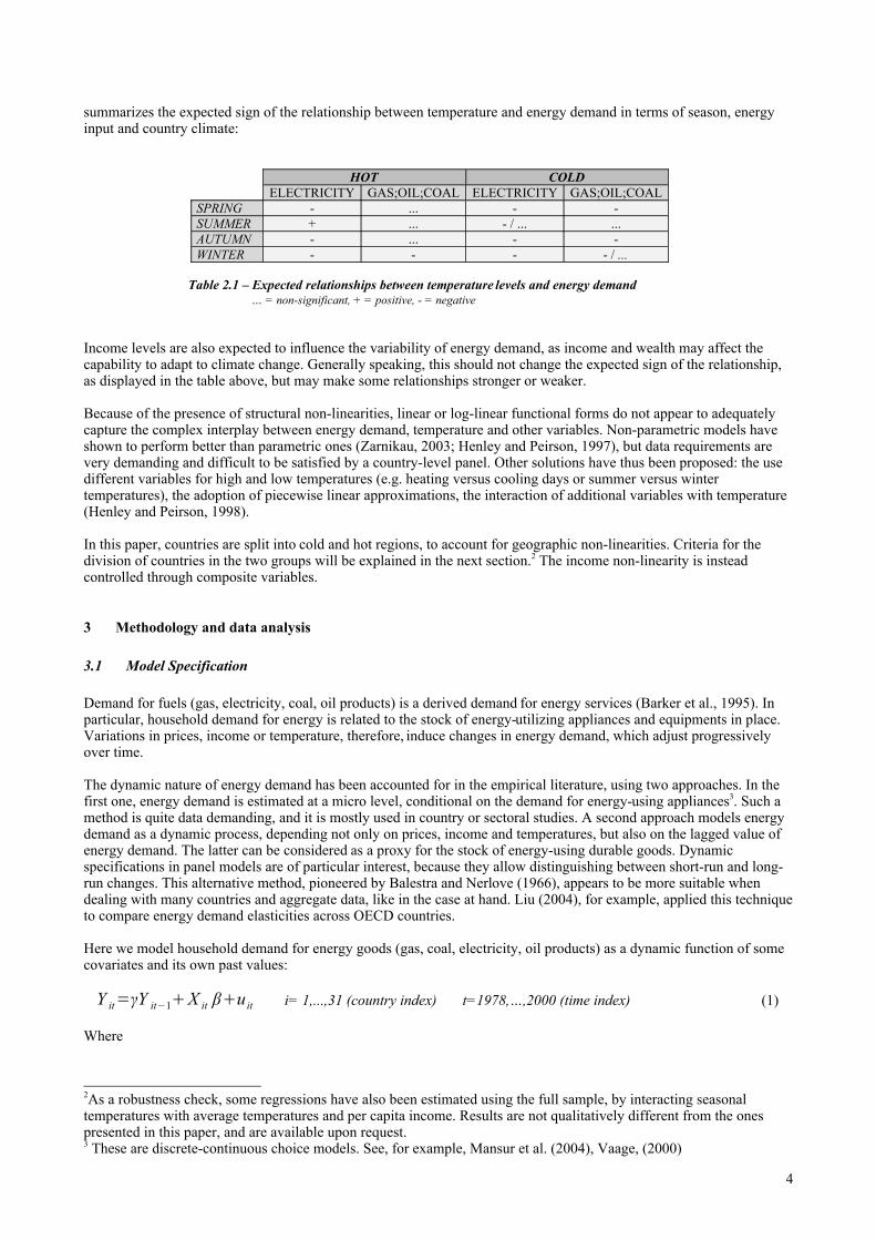
summarizes the expected sign of the relationship between temperature and energy demand in terms of season, energy input and country climate:

HOT COLDELECTRICITY GAS;OIL;COAL ELECTRICITY GAS;OIL;COAL

SPRING - ... - -SUMMER + ... - / ... ...AUTUMN - ... - -WINTER - - - - / ...

Table 2.1 – Expected relationships between temperature levels and energy demand ... = non-significant, + = positive, - = negative

Income levels are also expected to influence the variability of energy demand, as income and wealth may affect the capability to adapt to climate change. Generally speaking, this should not change the expected sign of the relationship, as displayed in the table above, but may make some relationships stronger or weaker.

Because of the presence of structural non-linearities, linear or log-linear functional forms do not appear to adequately capture the complex interplay between energy demand, temperature and other variables. Non-parametric models have shown to perform better than parametric ones (Zarnikau, 2003; Henley and Peirson, 1997), but data requirements are very demanding and difficult to be satisfied by a country-level panel. Other solutions have thus been proposed: the use different variables for high and low temperatures (e.g. heating versus cooling days or summer versus winter temperatures), the adoption of piecewise linear approximations, the interaction of additional variables with temperature (Henley and Peirson, 1998).

In this paper, countries are split into cold and hot regions, to account for geographic non-linearities. Criteria for the division of countries in the two groups will be explained in the next section.2 The income non-linearity is instead controlled through composite variables.

3 Methodology and data analysis

3.1 Model Specification

Demand for fuels (gas, electricity, coal, oil products) is a derived demand for energy services (Barker et al., 1995). In particular, household demand for energy is related to the stock of energy-utilizing appliances and equipments in place. Variations in prices, income or temperature, therefore, induce changes in energy demand, which adjust progressively over time.

The dynamic nature of energy demand has been accounted for in the empirical literature, using two approaches. In the first one, energy demand is estimated at a micro level, conditional on the demand for energy-using appliances3. Such a method is quite data demanding, and it is mostly used in country or sectoral studies. A second approach models energy demand as a dynamic process, depending not only on prices, income and temperatures, but also on the lagged value of energy demand. The latter can be considered as a proxy for the stock of energy-using durable goods. Dynamic specifications in panel models are of particular interest, because they allow distinguishing between short-run and long-run changes. This alternative method, pioneered by Balestra and Nerlove (1966), appears to be more suitable when dealing with many countries and aggregate data, like in the case at hand. Liu (2004), for example, applied this technique to compare energy demand elasticities across OECD countries.

Here we model household demand for energy goods (gas, coal, electricity, oil products) as a dynamic function of some covariates and its own past values:

Y it=γY it−1X it βu it i= 1,...,31 (country index) t=1978,…,2000 (time index) (1)

Where

2As a robustness check, some regressions have also been estimated using the full sample, by interacting seasonal temperatures with average temperatures and per capita income. Results are not qualitatively different from the ones presented in this paper, and are available upon request. 3 These are discrete-continuous choice models. See, for example, Mansur et al. (2004), Vaage, (2000)

4

Y it vector of dependent variables consisting of natural logarithm of household demands for gas, electricity, coal, and oil products;

Y it−1 vector of natural logarithm of the lagged dependent variables;X it covariates, including: natural logarithm of own and alternative energy good prices, average temperature

levels, real per capita GDP, real per capita GDP multiplied by temperature;u it=αiν it where ν it is IID (0,σ2) and αi is a country-specific factor.

Since all variables are in logarithmic form, the β coefficients are short-run elasticities, whereas long-run elasticities are defined for a stable value of Y it , that is for Y it=Y it−1 , which gives β /1−γ .

3.2 Data analysis

The sample used in this study is a data panel for 31 countries, covering the period 1978 – 20004. The data source on real GDP and energy residential demand is the International Energy Agency (IEA) - Energy Balances and Statistics. The fuels that are relevant for the residential sector are coal, natural gas, oil products and electricity. Demanded quantity is expressed in K toe. Fuel prices for the residential sector, measured in US$/toe, are obtained from the International Energy Agency (IEA) – Energy Prices and Taxes.5 To allow for cross-country comparisons, GDP is measured in Purchasing Power Parities (PPP) and prices are expressed in 1995 US$ equivalents. Temperature data has been obtained from the High Resolution Gridded Dataset of the Climatic Research Unit University of East Anglia and the from the Tyndall Centre for Climate Change Research.

This paper focuses solely on the residential sector. Several studies found that the industrial demand for energy does not respond very much to prices changes (Liu, 2002) and to temperature variations (Bigano et al., 2006; Asadoorian et al., 2006). Therefore, all data in the panel refer to the residential sector. Demand for electricity, gas, oil products, coal is measured in thousand of tonnes of oil equivalent (Toe). Real GDP has been converted into 1995 US$, using PPP. Energy prices are expressed in 1995 US$ per tonnes of oil equivalent (toe). Automotive diesel is used for oil products price, whereas steam coal price for coal. Temperatures are monthly or seasonal averages, expressed in Fahrenheit degrees.

Most series of energy demand appear to be either stationary or trend-stationary, except for electricity demand. Prices and temperature are stationary. To test for variable stationarity, different unit-root tests have been performed. In particular, the Fisher-type test for panel data developed by Maddala and Wu (1999) strongly rejects the non-stationarity of all variables, except the demand for electricity. These findings are not surprising and are in line with the analysis performed on a similar panel by Al-Rabbaie and Hunt (2005).

As the use of cooling devices in the hot season is a relatively recent phenomenon, the possible existence of structural breaks in the demand for electricity was considered. Therefore, a Wald test, following Greene (2000), was carried out. The test was repeated at different break points (years between 1994 and 1998, see Cooper et. al., 2003), and under different specifications. It was found that there is no significant difference between estimated parameters, so there is no need to model structural breaks.

3.3 Geographic variability of climate change: hot and cold countries

To better capture the two distinct effects of heating and cooling, hot and cold countries are separately considered. The division of the sample is based on the mean of the maximum monthly temperature in the year 2000. Cold countries are those having the maximum temperature below the mean, whereas hot countries have a maximum temperature above the average. The two sets and their related statistics are listed relatives in Table A1.1 and A1.2, Appendix 1.

There are no significant differences on real per capita GDP between cold and hot countries. In both sets, gas is the main energy input. However, whereas oil products are the second most important source of energy in cold countries, electricity is the second one in hot countries. This supports the hypothesis that electricity is more used in hot countries, because of the cooling effect. The hot countries subset contains a significant number of poor countries, making the variance of income higher. By making a further distinction between hot-rich and hot-poor countries (see tables A1.3 and A1.4, Appendix 1), we can see that the energy source mix is related both to the purpose (e.g., electricity for cooling, 4 The data set was provided by Andrea Bigano, Francesco Bosello and Giuseppe Marano, who are gratefully acknowledged. 5Data on energy prices is not consistent over time, countries and fuels. For this reason, the estimation of dynamic models is performed disregarding countries with many missing values. This procedure has lead to different sample sizes for each model.

5

other for heating) and to the income level. The intuition is that poor countries, despite generally having higher temperatures, cannot afford purchasing and using many air conditioners, as revealed by the relatively low electricity consumption.

3.4 Income variability of climate change

Per capita income is already included as an explanatory variable. However, in order to capture the possible interaction between income levels and sensitivity to changes in temperature, the product of temperature and income levels is experimented as an explanatory variable. In this way, the marginal effect of temperature on energy demand is directly influenced by per capita income. We expect a positive relationship between temperature elasticity of demand and income.

This kind of information, provided by the model, may be very valuable in applications of the model results for climate change policy and scenario analysis. Climate change will significantly affect the economy in the future, where many economic conditions (in particular, income levels) will be different from the ones characterizing the sample set used in this exercise.

3.5 Estimation method

The presence of a lagged dependent variable on the right-hand side of the regression equation, which is correlated with the error term, makes the OLS estimator biased and inconsistent. Given the stationarity of the series, the use of cointegration techniques is not indicated. In this context, the Arellano Bond method is a good alternative.

Dynamic models as the one described in section 3.1 exhibit two sources of persistence: the individual, unobservable effects and the state dependence between Y it and Y it−1 . These models do not satisfy the strict exogeneity assumption and, in addition, the correlation between the individual effect and Y it−1 is another source of inconsistency. For a sufficiently large time span of the series (T), Nickell (1981) shows that the Within Group estimator would yield an asymptotically consistent estimator. Alternatively, the unobservable effect can be eliminated by taking a first difference. This transformation, however, introduces a correlation between the differenced error term and the differenced covariates. Consistent estimators can be obtained using instrumental variables. Anderson and Hsiao (1981, 1982) proposed both the lagged levels and the lagged first differences as possible instruments. Arellano and Bond (1991) developed a generalized method of moments (GMM) estimator, using lagged levels of the dependent variable as instruments.

The estimation method proposed by Arellano and Bond has been chosen for three main reasons. First, it has proved to be quite efficient (Arellano and Bond, 1991). Secondly, it allows for the existence of an unobserved, country-specific effect, while relaxing the very strong hypothesis of strict exogeneity. This is important when dealing with a country panel, because including individual effects reduces the risk of bias due to omitted variables. Finally, the Arellano-Bond estimation can handle a flexible covariance matrix of the error terms, with possible serial correlation and heteroskedasticity.

In the estimations of the energy vector demand, the covariates are assumed to be endogenous:

E X it ,ν it ≠0 ∀ s≤t

The Arellano-Bond estimator delivers consistent and more efficient estimates when N is large and T is fixed, even if the panel is not balanced, as in this case. In this data set, the number of countries is not very big and the division of the sample into hot and cold countries increases the risk of finite sample bias. However, Arellano and Bond (1991), using Monte Carlo simulations, show that the finite sample bias of their estimator is smaller than those associated with alternative methods for dynamic models such as the Anderson and Hsiao estimator (1981, 1982) .

4 Results

Model (1) is estimated independently for each energy vector, using the one–step Arellano Bond estimator.6 As pointed out above, the number of instrument lags is limited to one, and all covariates are assumed to be endogenous. In this way, the number of instruments is restricted to those having a single lag, limiting as much as possible the reduction of the

6 The one-step is preferred to the two-steps estimator for inference, especially in small samples (Arellano and Bond, 1991).

6

sample size. For the estimations to be consistent, the error terms should display autocorrelation of first order, but not of second one. The xtabond command used to implement the Arellano bond estimator in the STATA software includes the test for autocorrelation and the Sargan test on the validity of the over-identifying restrictions. The absence of second order correlation ensures the consistency of the estimator.

The division of the sample into hot and cold countries accounts for the geographic variability. Two specifications are experimented: the first in which temperatures enter linearly (the basic version model) and a second one where temperatures are multiplied with income (the income interaction model).

4.1 The basic model

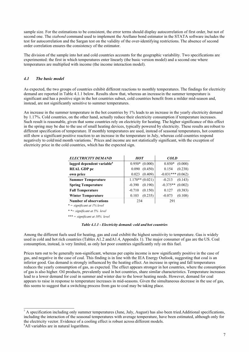
As expected, the two groups of countries exhibit different reactions to monthly temperatures. The findings for electricity demand are reported in Table 4.1.1 below. Results show that, whereas an increase in the summer temperature is significant and has a positive sign in the hot countries subset, cold countries benefit from a milder mid-season and, instead, are not significantly sensitive to summer temperatures.

An increase in the summer temperature in the hot countries by 1% leads to an increase in the yearly electricity demand by 1.17%. Cold countries, on the other hand, actually reduce their electricity consumption if temperature increases. Such result is reasonable, given that some countries rely on electricity for heating. The higher significance of this effect in the spring may be due to the use of small heating devices, typically powered by electricity. These results are robust to different specification of temperature. If monthly temperatures are used, instead of seasonal temperatures, hot countries still show a significant positive reaction to an increase in the temperature in July, whereas cold countries respond negatively to cold/mid month variations.7 Prices and income are not statistically significant, with the exception of electricity price in the cold countries, which has the expected sign.

ELECTRICITY DEMAND HOT COLDlagged dependent variable8 0.950* (0.000) 0.850* (0.000)REAL GDP pc 0.090 (0.450) 0.154 (0.238)own price 0.023 (0.409) -0.031*** (0.062)Summer Temperature 1.170** (0.021) -0.213 (0.143)Spring Temperature -0.390 (0.190) -0.375** (0.002)Fall Temperature -0.710 (0.150) 0.127 (0.383)Winter Temperature 0.103 (0.235) -0.073 (0.108)Number of observations 234 291

* = significant at 1% level* *= significant at 5% level*** = significant at 10% level

Table 4.1.1 - Electricity demand: cold and hot countries

Among the different fuels used for heating, gas and coal exhibit the highest sensitivity to temperature. Gas is widely used in cold and hot rich countries (Tables A1.2 and A1.4, Appendix 1). The major consumer of gas are the US. Coal consumption, instead, is very limited, as only hot poor countries significantly rely on this fuel.

Prices turn out to be generally non-significant, whereas per capita income is now significantly positive in the case of gas, and negative in the case of coal. This finding is in line with the IEA Energy Outlook, suggesting that coal is an inferior good. Gas demand is strongly influenced by the heating effect. An increase in spring and fall temperatures reduces the yearly consumption of gas, as expected. The effect appears stronger in hot countries, where the consumption of gas is also higher. Oil products, prevalently used in hot countries, share similar characteristics. Temperature increases lead to a lower demand for coal in summer and winter due to the lower heating needs. However, demand for coal appears to raise in response to temperature increases in mid-seasons. Given the simultaneous decrease in the use of gas, this seems to suggest that a switching process from gas to coal may be taking place.

7 A specification including only summer temperatures (June, July, August) has also been tried. Additional specifications, including the interaction of the seasonal temperatures with average temperature, have been estimated, although only for the electricity vector. Evidence of a cooling effect is robust across different models. 8All variables are in natural logarithms.

7

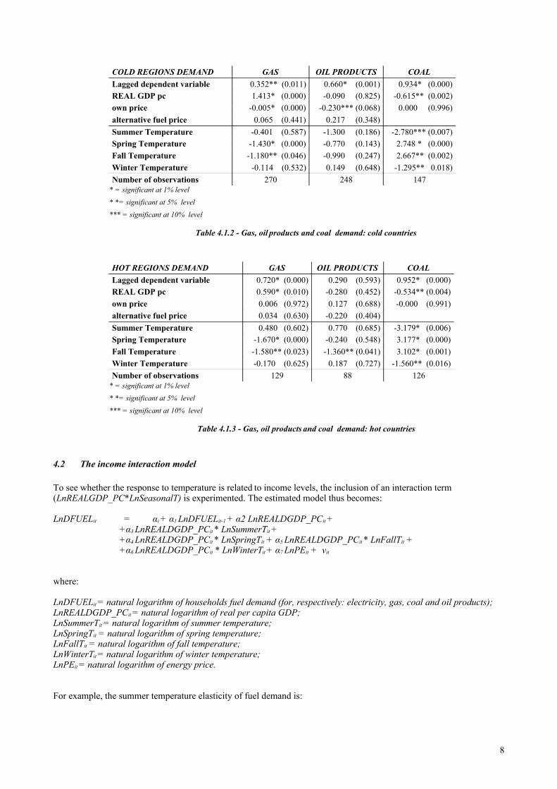
COLD REGIONS DEMAND GAS OIL PRODUCTS COALLagged dependent variable 0.352** (0.011) 0.660* (0.001) 0.934* (0.000)REAL GDP pc 1.413* (0.000) -0.090 (0.825) -0.615** (0.002)own price -0.005* (0.000) -0.230*** (0.068) 0.000 (0.996)alternative fuel price 0.065 (0.441) 0.217 (0.348) Summer Temperature -0.401 (0.587) -1.300 (0.186) -2.780*** (0.007)Spring Temperature -1.430* (0.000) -0.770 (0.143) 2.748 * (0.000)Fall Temperature -1.180** (0.046) -0.990 (0.247) 2.667** (0.002)Winter Temperature -0.114 (0.532) 0.149 (0.648) -1.295** 0.018)Number of observations 270 248 147

* = significant at 1% level* *= significant at 5% level*** = significant at 10% level

Table 4.1.2 - Gas, oil products and coal demand: cold countries

HOT REGIONS DEMAND GAS OIL PRODUCTS COALLagged dependent variable 0.720* (0.000) 0.290 (0.593) 0.952* (0.000)REAL GDP pc 0.590* (0.010) -0.280 (0.452) -0.534** (0.004)own price 0.006 (0.972) 0.127 (0.688) -0.000 (0.991)alternative fuel price 0.034 (0.630) -0.220 (0.404) Summer Temperature 0.480 (0.602) 0.770 (0.685) -3.179* (0.006)Spring Temperature -1.670* (0.000) -0.240 (0.548) 3.177* (0.000)Fall Temperature -1.580** (0.023) -1.360** (0.041) 3.102* (0.001)Winter Temperature -0.170 (0.625) 0.187 (0.727) -1.560** (0.016)Number of observations 129 88 126

* = significant at 1% level* *= significant at 5% level*** = significant at 10% level

Table 4.1.3 - Gas, oil products and coal demand: hot countries

4.2 The income interaction model

To see whether the response to temperature is related to income levels, the inclusion of an interaction term (LnREALGDP_PC*LnSeasonalT) is experimented. The estimated model thus becomes:

LnDFUELit = αi + α1 LnDFUELit-1 + α2 LnREALDGDP_PCit ++α3 LnREALDGDP_PCit * LnSummerTit ++α4 LnREALDGDP_PCit * LnSpringTit + α5 LnREALDGDP_PCit * LnFallTit ++α6 LnREALDGDP_PCit * LnWinterTit + α7 LnPEit + νit

where:

LnDFUELit = natural logarithm of households fuel demand (for, respectively: electricity, gas, coal and oil products);LnREALDGDP_PCit = natural logarithm of real per capita GDP;LnSummerTit = natural logarithm of summer temperature;LnSpringTit = natural logarithm of spring temperature;LnFallTit = natural logarithm of fall temperature;LnWinterTit = natural logarithm of winter temperature;LnPEit = natural logarithm of energy price.

For example, the summer temperature elasticity of fuel demand is:

8

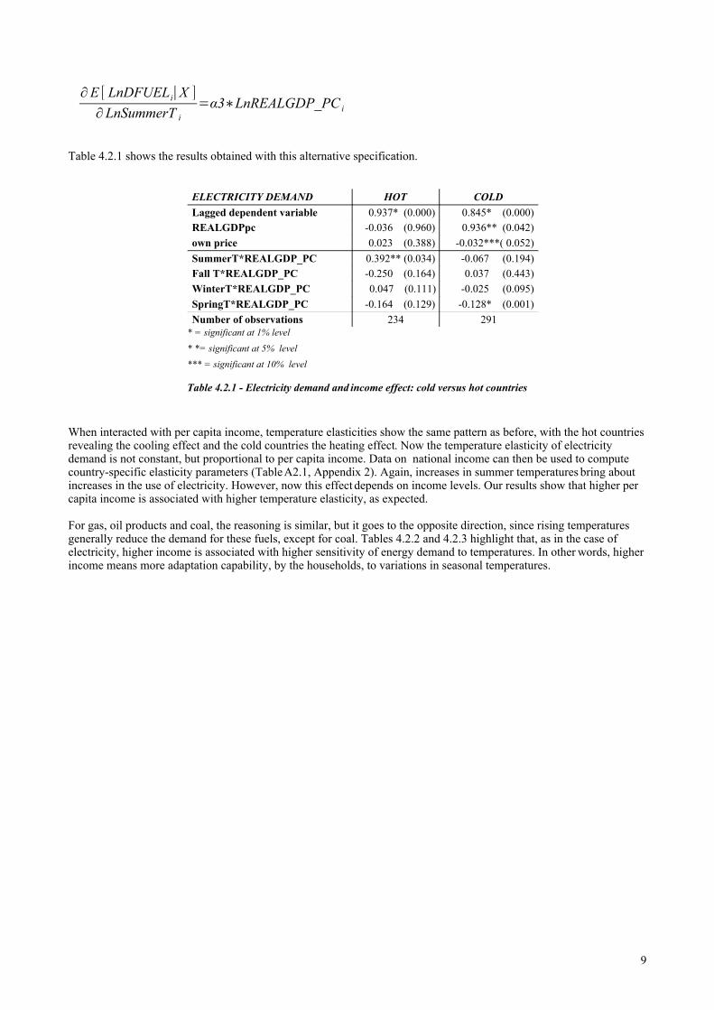
∂E [ LnDFUELi∣X ]∂LnSummerT i

=α3∗LnREALGDP_PC i

Table 4.2.1 shows the results obtained with this alternative specification.

ELECTRICITY DEMAND HOT COLDLagged dependent variable 0.937* (0.000) 0.845* (0.000)REALGDPpc -0.036 (0.960) 0.936** (0.042)own price 0.023 (0.388) -0.032***( 0.052)SummerT*REALGDP_PC 0.392** (0.034) -0.067 (0.194)Fall T*REALGDP_PC -0.250 (0.164) 0.037 (0.443)WinterT*REALGDP_PC 0.047 (0.111) -0.025 (0.095)SpringT*REALGDP_PC -0.164 (0.129) -0.128* (0.001)Number of observations 234 291

* = significant at 1% level* *= significant at 5% level*** = significant at 10% level

Table 4.2.1 - Electricity demand and income effect: cold versus hot countries

When interacted with per capita income, temperature elasticities show the same pattern as before, with the hot countries revealing the cooling effect and the cold countries the heating effect. Now the temperature elasticity of electricity demand is not constant, but proportional to per capita income. Data on national income can then be used to compute country-specific elasticity parameters (Table A2.1, Appendix 2). Again, increases in summer temperatures bring about increases in the use of electricity. However, now this effect depends on income levels. Our results show that higher per capita income is associated with higher temperature elasticity, as expected.

For gas, oil products and coal, the reasoning is similar, but it goes to the opposite direction, since rising temperatures generally reduce the demand for these fuels, except for coal. Tables 4.2.2 and 4.2.3 highlight that, as in the case of electricity, higher income is associated with higher sensitivity of energy demand to temperatures. In other words, higher income means more adaptation capability, by the households, to variations in seasonal temperatures.

9

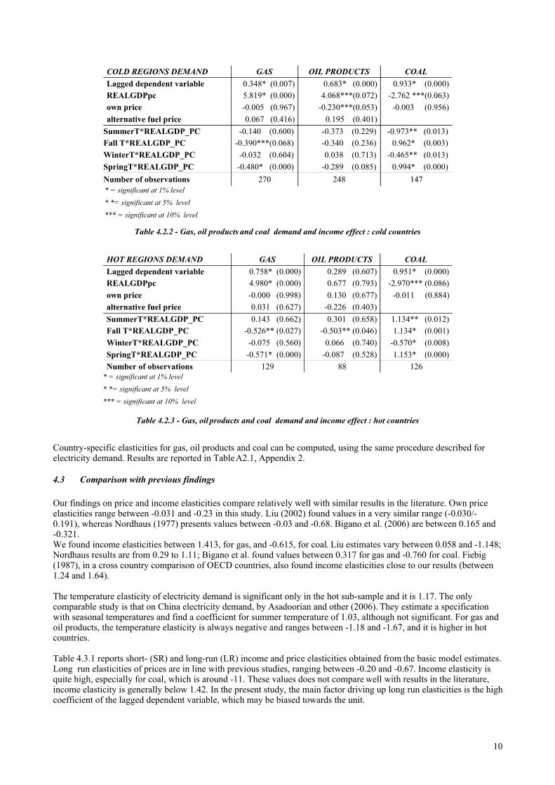
COLD REGIONS DEMAND GAS OIL PRODUCTS COALLagged dependent variable 0.348* (0.007) 0.683* (0.000) 0.933* (0.000)REALGDPpc 5.819* (0.000) 4.068***(0.072) -2.762 ***(0.063)own price -0.005 (0.967) -0.230***(0.053) -0.003 (0.956)alternative fuel price 0.067 (0.416) 0.195 (0.401)

SummerT*REALGDP_PC -0.140 (0.600) -0.373 (0.229) -0.973** (0.013)Fall T*REALGDP_PC -0.390***(0.068) -0.340 (0.236) 0.962* (0.003)WinterT*REALGDP_PC -0.032 (0.604) 0.038 (0.713) -0.465** (0.013)SpringT*REALGDP_PC -0.480* (0.000) -0.289 (0.085) 0.994* (0.000)Number of observations 270 248 147* = significant at 1% level* *= significant at 5% level*** = significant at 10% level

Table 4.2.2 - Gas, oil products and coal demand and income effect : cold countries

HOT REGIONS DEMAND GAS OIL PRODUCTS COALLagged dependent variable 0.758* (0.000) 0.289 (0.607) 0.951* (0.000)REALGDPpc 4.980* (0.000) 0.677 (0.793) -2.970*** (0.086)own price -0.000 (0.998) 0.130 (0.677) -0.011 (0.884)alternative fuel price 0.031 (0.627) -0.226 (0.403) SummerT*REALGDP_PC 0.143 (0.662) 0.301 (0.658) 1.134** (0.012)Fall T*REALGDP_PC -0.526** (0.027) -0.503** (0.046) 1.134* (0.001)WinterT*REALGDP_PC -0.075 (0.560) 0.066 (0.740) -0.570* (0.008)SpringT*REALGDP_PC -0.571* (0.000) -0.087 (0.528) 1.153* (0.000)Number of observations 129 88 126

* = significant at 1% level* *= significant at 5% level*** = significant at 10% level

Table 4.2.3 - Gas, oil products and coal demand and income effect : hot countries

Country-specific elasticities for gas, oil products and coal can be computed, using the same procedure described for electricity demand. Results are reported in Table A2.1, Appendix 2.

4.3 Comparison with previous findings

Our findings on price and income elasticities compare relatively well with similar results in the literature. Own price elasticities range between -0.031 and -0.23 in this study. Liu (2002) found values in a very similar range (-0.030/-0.191), whereas Nordhaus (1977) presents values between -0.03 and -0.68. Bigano et al. (2006) are between 0.165 and -0.321. We found income elasticities between 1.413, for gas, and -0.615, for coal. Liu estimates vary between 0.058 and -1.148; Nordhaus results are from 0.29 to 1.11; Bigano et al. found values between 0.317 for gas and -0.760 for coal. Fiebig (1987), in a cross country comparison of OECD countries, also found income elasticities close to our results (between 1.24 and 1.64).

The temperature elasticity of electricity demand is significant only in the hot sub-sample and it is 1.17. The only comparable study is that on China electricity demand, by Asadoorian and other (2006). They estimate a specification with seasonal temperatures and find a coefficient for summer temperature of 1.03, although not significant. For gas and oil products, the temperature elasticity is always negative and ranges between -1.18 and -1.67, and it is higher in hot countries.

Table 4.3.1 reports short- (SR) and long-run (LR) income and price elasticities obtained from the basic model estimates. Long run elasticities of prices are in line with previous studies, ranging between -0.20 and -0.67. Income elasticity is quite high, especially for coal, which is around -11. These values does not compare well with results in the literature, income elasticity is generally below 1.42. In the present study, the main factor driving up long run elasticities is the high coefficient of the lagged dependent variable, which may be biased towards the unit.

10

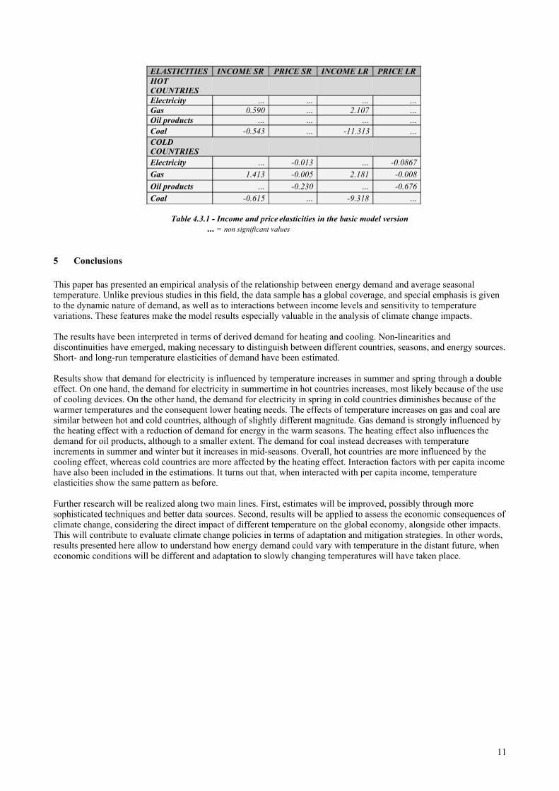
ELASTICITIES INCOME SR PRICE SR INCOME LR PRICE LRHOT COUNTRIES

Electricity … … … …Gas 0.590 … 2.107 …Oil products … … … …Coal -0.543 … -11.313 …COLD COUNTRIES

Electricity … -0.013 … -0.0867Gas 1.413 -0.005 2.181 -0.008Oil products … -0.230 … -0.676Coal -0.615 … -9.318 …

Table 4.3.1 - Income and price elasticities in the basic model version ... = non significant values

5 Conclusions

This paper has presented an empirical analysis of the relationship between energy demand and average seasonal temperature. Unlike previous studies in this field, the data sample has a global coverage, and special emphasis is given to the dynamic nature of demand, as well as to interactions between income levels and sensitivity to temperature variations. These features make the model results especially valuable in the analysis of climate change impacts.

The results have been interpreted in terms of derived demand for heating and cooling. Non-linearities and discontinuities have emerged, making necessary to distinguish between different countries, seasons, and energy sources. Short- and long-run temperature elasticities of demand have been estimated.

Results show that demand for electricity is influenced by temperature increases in summer and spring through a double effect. On one hand, the demand for electricity in summertime in hot countries increases, most likely because of the use of cooling devices. On the other hand, the demand for electricity in spring in cold countries diminishes because of the warmer temperatures and the consequent lower heating needs. The effects of temperature increases on gas and coal are similar between hot and cold countries, although of slightly different magnitude. Gas demand is strongly influenced by the heating effect with a reduction of demand for energy in the warm seasons. The heating effect also influences the demand for oil products, although to a smaller extent. The demand for coal instead decreases with temperature increments in summer and winter but it increases in mid-seasons. Overall, hot countries are more influenced by the cooling effect, whereas cold countries are more affected by the heating effect. Interaction factors with per capita income have also been included in the estimations. It turns out that, when interacted with per capita income, temperature elasticities show the same pattern as before.

Further research will be realized along two main lines. First, estimates will be improved, possibly through more sophisticated techniques and better data sources. Second, results will be applied to assess the economic consequences of climate change, considering the direct impact of different temperature on the global economy, alongside other impacts. This will contribute to evaluate climate change policies in terms of adaptation and mitigation strategies. In other words, results presented here allow to understand how energy demand could vary with temperature in the distant future, when economic conditions will be different and adaptation to slowly changing temperatures will have taken place.

11

References

Al-Rabbaie, A. and L. C. Hunt (2005) OECD Energy Demand: Modeling Energy Demand Trends using Structural Time Series Model, paper presented at the USAEE/IAEE North American Conference, Denver, Co., USA.

Arellano, M. and S. Bond (1991) Some Tests of Specification for Panel Data: Monte Carlo Evidence and an Application to Employment Equations, The Review of Economic Studies, 58(2), 227-297.

Asadoorian O. M., R. Eckaus and C.A. Schlosser (2006) Modeling Climate feedbacks to Energy Demand: The Case of China, MIT Joint Program on the Science and Policy of Global Change, Report No. 135.

Balestra, P. and M. Nerlove (1966) Pooling cross-section and time-series data in the estimation of a dynamic model: The demand for natural gas, Econometrica, 31, 585-612.

Barker T., P. Ekins and N. Johnstone (1995) Global Warming and Energy Demand, London, Routledge Global Environmental Change Book Series.

Berrittella, M., A. Bigano, R. Roson and R.S.J. Tol (2006) A General Equilibrium Analysis of Climate Change Impacts on Tourism, Tourism Management, 25(5), 913-924

Bigano, A., F. Bosello and G. Marano (2006) Energy demand and temperature: a dynamic panel analysis, Fondazione ENI Enrico Mattei Working Paper No. 112.06.

Bosello, F., R. Roson and R.S.J. Tol (2006) Economy-Wide Estimates of the Implications of Climate Change: Human Health, Ecological Economics, 58(3), 579-591.

Bosello, F., R. Roson and R.S.J. Tol (2007) Economy-Wide Estimates of the Implications of Climate Change: Sea Level Rise, Environmental and Resource Economics, forthcoming.

Bosello, F. and J. Zhang (2005) Assessing Climate Change Impacts: Agriculture, Fondazione ENI Enrico Mattei Working Paper No. 94.05.

Calzadilla, A., F. Pauli and R. Roson (2006) Climate Change and Extreme Events: An Assessment of Economic Implications, International Journal of Ecological Economics and Statistics, forthcoming.

Cline, W. (1992) The Economics of Global Warming Institute for International Economics, Washington.

Cooper, S.J., D. M. Kennedy and A. A. Braga (2003) Testing for Structural Breaks in the Evaluation of Programs, Review of Economics and Statistics, 85(3), 550-558.

Fiebig, D.G., J. Seale, J. and H. Theil (1978) The demand for energy: evidence from cross-country demand system, Energy Economics 15, 9-16.

Greene, W. (2000) Econometric Analysis, 4th ed., London, Prentice-Hall International.

Henley, A., and J. Peirson (1996) Energy pricing and temperature interaction: British experimental evidence. Aberystwyth Economic Research Paper, No. 96-16, University of Wales Aberystwyth.

Henley, A., and J. Peirson (1997) Non-linearities in electricity demand and temperature: parametric vs.non-parametric methods. Oxford Bulletin of Economic and Statistic, 59, 149-162.

Henley, A. and J. Peirson (1998) Residential energy demand and the interaction of price temperature: British experimental evidence. Energy Economics, 20, 157-171.

Liu, G. (2004) Estimating Energy Demand Elasticities for OECD Countries – A Dynamic Panel Data Approach, Discussion Papers No. 373, Statistics Norway, Research Department.

Madlener R. and R. Alt (1996) Residential Energy Demand Analysis: An EmpiricalApplication of the Closure Test Principle. Empirical Economics, 21, 203-220.

Mansur E.T., R. Mendelsohn, and W. Morrison (2004) A Discrete-Continuous Choice Model of Climate Change Impacts on Energy, Yale SOM Working Paper No. ES-43.

12

Moral–Carcedo J. and J. Vicens-Otero (2005) Modeling the non-linear response of Spanish electricity demand to temperature variations, Energy Economics, Vol. 27, pg. 477-494.

Nickell, S. (1981) Biases in dynamic models with fixed effects, Econometrica 49, 1471-1426

Nordhaus, W.D. (1977) The demand for energy: an international perspective, in Nordhaus W.D.(ed.) International Studies of the Demand for Energy. Amsterdam: North Holland.

Parti P. and C. Parti (1980) The Total and Appliance-Specific Conditional Demand for Electricity in the Household Sector. The Bell Journal of Economics, 11, 309-321.

Pindyck, R.S. (2006) Uncertainty in Environmental Economics, NBER working paper 12752, December 2006.

Rosenthal, D. H. and H. K. Gruenspecht (1995) Effects of global warming on energy use for space heating and cooling in the United States, Energy Journal,, 16(2), 77-20.

Smith, S. (1992) Distributional effects of a European carbon tax, Fondazione ENI Enrico Mattei Working Paper No. 22.92.

Smith, J.B. And D.A. Tirpak (1989) The Potential Effects of Global Climate Change on the United States, EPA-230-05-89-05, USEPA, Office of Policy, Planning and Evaluation, Washington, DC.

Stephan G., R. van Nieuwkoup and T. Weidmer (1993) Social incidence and economic costs of carbon limits, Universitat Bern, Volkswirtschaftliches Institut, Discussion Paper No. 9201.

Vaage, K. (2000) Heating technology and energy use: a discrete/continuous choice approach to Norwegian household energy demand, Energy Economics, 22, 649-666.

13

Appendix 1: Data Analysis

Table A1.1 - Division of the sample into cold and hot countriesMean of the maximum monthly temperature: 90,99290

COLD HOTAUSTRIA AUSTRALIABELGIUM SPAINCANADA GREECESWITZERLAND HUNGARYGERMANY INDONESIADENMARK INDIAFINLAND ITALYFRANCE JAPANIRELAND KOREALUXEMBURG MEXICONETHERLANDS PORTUGAL NORWAY THAILANDNEW ZELAND TURKEYSWEDEN UNITED STATESUNITED KINGDOM VENEZUELA SOUTH AFRICA

Table A1.2: Mean values of main variablesMean values (Std deviation) Cold HotMax temp 82.69 (4.08) 98.50 (4.68)LnReal GDP PC 2.54 (0.24) 2.15 (0.81)Gas 5882.54 (9690) 21813.34 (38367)Electricity 3507.36 (5665) 7180.31 (18442)Oil Products 3810.71 (5947) 6214.83 (9061)Coal 1056.72 (2306) 1277.00 (2412)

Table A1.3: Division of the sample into hot-rich and hot-poor countriesHot rich Hot poorAUSTRALIA INDONESIASPAIN INDIAGREECE VENEZUELAHUNGARY MEXICOSOUTH AFRICA THAILANDPORTUGAL TURKEYITALYJAPANKOREAUNITED STATES

Table A1.4: Mean values of main variables Mean values (Std deviation) Hot rich Hot poorMax temp 96.37 (3.68) 101.56 (4.27)LnReal GDP PC 2.72 (0.33) 1.33 (0.58)Gas 21813.34 (38367.78)Electricity 11283.94 (23157.93) 1294.83 (1144.55)Oil Products 7496.39 (11022.46) 4376.80 (4502.56)Coal 572.85 (788.54) 2286.89 (3404.29)

14

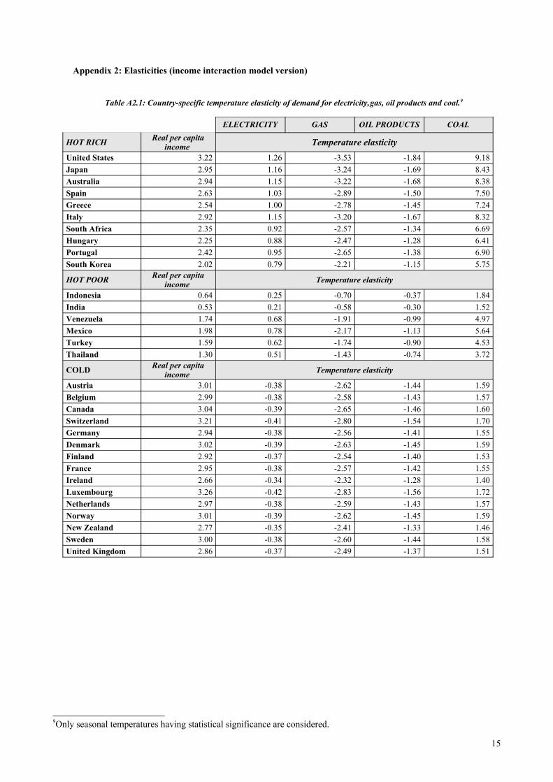
Appendix 2: Elasticities (income interaction model version)

Table A2.1: Country-specific temperature elasticity of demand for electricity, gas, oil products and coal.9

ELECTRICITY GAS OIL PRODUCTS COAL

HOT RICH Real per capita income Temperature elasticity

United States 3.22 1.26 -3.53 -1.84 9.18Japan 2.95 1.16 -3.24 -1.69 8.43Australia 2.94 1.15 -3.22 -1.68 8.38Spain 2.63 1.03 -2.89 -1.50 7.50Greece 2.54 1.00 -2.78 -1.45 7.24Italy 2.92 1.15 -3.20 -1.67 8.32South Africa 2.35 0.92 -2.57 -1.34 6.69Hungary 2.25 0.88 -2.47 -1.28 6.41Portugal 2.42 0.95 -2.65 -1.38 6.90South Korea 2.02 0.79 -2.21 -1.15 5.75

HOT POOR Real per capita income Temperature elasticity

Indonesia 0.64 0.25 -0.70 -0.37 1.84India 0.53 0.21 -0.58 -0.30 1.52Venezuela 1.74 0.68 -1.91 -0.99 4.97Mexico 1.98 0.78 -2.17 -1.13 5.64Turkey 1.59 0.62 -1.74 -0.90 4.53Thailand 1.30 0.51 -1.43 -0.74 3.72

COLD Real per capita income Temperature elasticity

Austria 3.01 -0.38 -2.62 -1.44 1.59Belgium 2.99 -0.38 -2.58 -1.43 1.57Canada 3.04 -0.39 -2.65 -1.46 1.60Switzerland 3.21 -0.41 -2.80 -1.54 1.70Germany 2.94 -0.38 -2.56 -1.41 1.55Denmark 3.02 -0.39 -2.63 -1.45 1.59Finland 2.92 -0.37 -2.54 -1.40 1.53France 2.95 -0.38 -2.57 -1.42 1.55Ireland 2.66 -0.34 -2.32 -1.28 1.40Luxembourg 3.26 -0.42 -2.83 -1.56 1.72Netherlands 2.97 -0.38 -2.59 -1.43 1.57Norway 3.01 -0.39 -2.62 -1.45 1.59New Zealand 2.77 -0.35 -2.41 -1.33 1.46Sweden 3.00 -0.38 -2.60 -1.44 1.58United Kingdom 2.86 -0.37 -2.49 -1.37 1.51

9Only seasonal temperatures having statistical significance are considered.

15