The Impact of Past Epidemics on Future

Disease Dynamics

Shweta Bansal∗†‡, Lauren Ancel Meyers§¶

October 13, 2009

Abstract

Many pathogens spread primarily via direct contact between infected

and susceptible hosts. Thus, the patterns of contacts or contact network

of a population fundamentally shapes the course of epidemics. While

there is a robust and growing theory for the dynamics of single epidemics

in networks, we know little about the impacts of network structure on

long term epidemic or endemic transmission. For seasonal diseases like

in�uenza, pathogens repeatedly return to populations with complex and

changing patterns of susceptibility and immunity acquired through prior

infection. Here, we develop two mathematical approaches for modeling

consecutive seasonal outbreaks of a partially-immunizing infection in a

population with contact heterogeneity. Using methods from percolation

theory we consider both leaky immunity, where all previously infected

individuals gain partial immunity, and perfect immunity, where a fraction

of previously infected individuals are fully immune. By restructuring the

epidemiologically active portion of their host population, such diseases

limit the potential of future outbreaks. We speculate that these dynamics

can result in evolutionary pressure to increase infectiousness.

1 Introduction

Immunity acquired via infection gives an individual protection from subsequentinfection by the same or similar pathogen for some period of time. For diseasessuch as measles, varicella (chickenpox), mumps and rubella, complete immu-nity lasts a lifetime; therefore an individual who has been infected by one ofthese pathogens, once recovered, cannot be reinfected, nor transmit the infec-tion again. For other diseases, immunity wanes with time, leaving previously

∗Center for Infectious Disease Dynamics, The Pennsylvania State University, 208 Mueller

Lab, University Park PA 16802†Fogarty International Center, National Institutes of Health, Bethesda, MD 20892, USA‡Corresponding Author: shweta@sbansal.com§Section of Integrative Biology and Institute for Cellular and Molecular Biology, University

of Texas at Austin, 1 University Station, C0930, Austin, TX 78712, USA¶Santa Fe Institute, 1399 Hyde Park Road, Santa Fe, NM 87501, USA

1

arX

iv:0

910.

2008

v1 [

q-bi

o.PE

] 1

2 O

ct 2

009

infected individuals only partially protected against reinfection (called partial

immunity). This degradation of immunity may be caused by antigenic variationin the circulating pathogen or loss of antibodies over time. The transition fromcomplete to partial immunity can happen over di�erent timescales: over a fewweeks as with norovirus and rotavirus [41], over months or a few years as within�uenza [20], or over many years as with pertussis [38]. Here, we present newmethods for modeling the epidemiological consequences of partial immunity.

Although partial immunity is not well-understood, there is evidence thatpartial immunity functions in one of two ways: leaky or perfect. For a de-gree of partial immunity q, leaky partial immunity implies that each immunizedindividual reduces their chances of getting reinfected and infecting others bya proportion q, whereas perfect partial immunity implies that a fraction q ofimmunized individuals enjoy full protection from reinfection and the remain-ing (1− q) proportion are completely susceptible. Leaky partial immunity isexpected to be the more common of the two, and more consistent with ourunderstanding of the immune system [22]. Perfect partial immunity is less com-mon, but can occur if some individuals are unable to mount a lasting immuneresponse to an otherwise fully immunizing disease. It has been observed, forexample, in vaccine and animal studies for varicella, meningococcal infection[12], and Hepatitis C [10, 15].

Partial immunity may impact the host in multiple ways, and have far-reaching implications for the transmission of a disease through a population.Speci�cally, it can decrease one or both of two fundamental epidemiologicalquantities: infectivity, the probability that an infected individual will infect asusceptible individual with whom he or she has contact; and susceptibility, theprobability that a susceptible individual will be infected if exposed to diseasevia contact with an infected individual. In mathematical models, the probabil-ity of transmission (transmissibility) during a contact between an infected andsusceptible individual is often represented as a product of the infectivity of theinfected node and the susceptibility of the susceptible node. Partial immunitycan limit transmissibility either by lowering the probability of reinfection or re-ducing the degree to which an infected individual sheds the pathogen. Both, forexample, occur in the case of in�uenza [36, 13].

Mathematical modeling of infectious disease dynamics has been dominatedby the Susceptible-Infected-Recovered (SIR) compartmental model [23] whichconsiders infectious disease transmission in a closed population of individualswho enjoy complete immunity following infection. The SIR model has been ex-tended to Susceptible-Infected-Recovered-Susceptible (SIRS) dynamics to modelthe full loss of complete immunity after a temporary period of protection [21, 39],and has been applied successfully in several situations (e.g. [19]). Models ofpartially immunizing pathogens are less common, and have primarily been de-veloped for particular pathogens, such as in�uenza [34, 24, 29]. They con-sider the impacts of antigenic variation and the resulting complex patterns ofcross-immunity on epidemic dynamics, but are limited by the assumptions ofhomogeneous-mixing.

Contact network epidemiology is a tractable and powerful mathematical ap-

2

proach that goes beyond homogeneous-mixing and explicitly captures the di-verse patterns of interactions that underlie disease transmission [5, 40, 31, 25,35, 4]. In this framework, the host population is represented by a network ofindividuals (each represented by a node) and the disease-causing contacts (rep-resented by edges) between them (Figure 1(a)). The number of contacts (edges)of a node is called its degree, and the distribution of degrees throughout the net-work fundamentally in�uences where and when a disease will spread [25, 27, 4].The traditional SIR model has been mapped to a bond percolation process on acontact network, in which individuals independently progress through S, I, andR stages if and when disease reaches their location in the network [27]. Thebond percolation threshold corresponds to the epidemic threshold, above whichan epidemic outbreak is possible (i.e. one that infects a non-zero fraction of thepopulation, in the limit of large populations); and the size of the percolatingcluster (or giant component) above this transition corresponds to the size ofthe epidemic. The standard bond percolation model for disease spread througha network, however, assumes a completely naive population without immunityfrom prior epidemics [27].

In this paper, we extend the bond percolation framework to consider theimpact of infection-acquired immunity on epidemiological dynamics. We modelboth perfect (Section 2.1) and leaky (Section 2.2) partial immunity, and showthat the two models are identical in the cases of no immunity or complete im-munity, but make very di�erent predictions for partial immunity. The evolutionof infectiousness, virulence and a pathogen's antigenic characteristics are in partdriven by the epidemiological environment. Although signi�cant attention hasbeen paid to the interaction between contact network structure and pathogenevolution and competition [8, 33, 37, 9, 28], we do not yet understand the inter-seasonal interactions via modi�cation to the immunological structure of the hostcontact network. Feedback from an evolving organism to its own ecological andevolutionary environment is generally known as niche construction [30, 7]. Here,we use our models to explore a particular instance of niche construction: theimpacts of prior epidemics on the future dynamics of the pathogen.

2 Methods: Incorporating Infection-Acquired Im-

munity into a Network Model

We present two mathematical approaches to modeling partial immunity. First,we model perfect partial immunity by completely removing a fraction of the in-dividuals (their nodes and edges) who are infected during an epidemic (Figure1(b)) from the network.Using the bond percolation model, we then derive epi-demiological quantities for a subsequent outbreak in the immunized population.Second, we model leaky partial immunity using a new two-type percolationmodel. The underlying contact network topology remains intact, but nodesare classi�ed either as partially immune or susceptible (Figure 1(c)). In bothmodels, we assume that both infectivity and susceptibility are reduced due to

3

immunity, but the leaky partial immunity model can be easily adapted to modelother e�ects of immunity.

Below, we use both models to consider dynamics in three network types: (a)Poisson, with degree distribution pk = e−λλk/k!; (b) exponential, with degreedistribution pk = (1 − eκ)e−κ(k−1); and (c) scale-free, with degree distributionpk = k−γ/ζ(γ), each with a mean degree of 10. All model predictions areveri�ed using stochastic simulations which assume a simple percolation processwith parameters to match the model.

2.1 Perfect Partial Immunity

Perfect partial immunity, sometimes known as �all-or-nothing� partial immu-nity or polarized immunity, implies that for a partial immunity level (1− α), afraction (1− α) of the infected population are fully immune to reinfection (andthus transmitting to others) and the remaining proportion α are fully vulnera-ble to reinfection (and transmission to others thereafter.) In terms of a contactnetwork, this means that a fraction of the previously infected nodes are nowcompletely removed (along with its edges) from the contact network and are nolonger a part of the transmission process. The residual network, introduced in[16, 3] models this phenomenon. Previously, we characterized the residual net-work as the network made up of uninfected individuals and the edges connectingthem, as we assumed that all infected individuals had gained full immunity toinfection and thus could be fully removed (along with their edges) from thetransmission chain of future epidemics. Now, we extend the description of theresidual network to include not only uninfected nodes, but also nodes that werepreviously infected but have already lost immunity. We apply bond percolationmethods to this extended residual network to model the spread of a subsequentoutbreak in a population that has already su�ered an initial outbreak.

The simple Susceptible-Infectious-Recovered (SIR) bond percolation modelallows us to derive fundamental epidemiological quantities based on the aver-age transmissibility T of the pathogen (that is, the average probability that aninfected node will transmit to a susceptible contact sometime during its infec-tious period) and the degree distribution of the host contact network, denoted{pk} where pk is the fraction of nodes with degree k [27]. This assumes thatthe probabilities of transmission from infected nodes to susceptible nodes are iidrandom variables. We can then calculate the epidemic threshold for a given net-work (Tc), above which a large scale epidemic is possible; this is closely relatedto the traditional epidemiological quantity, R0. We can also �nd the probabilityand expected size of an epidemic above that threshold as well as the probabilitythat an individual at the end of a randomly chosen edge (contact) does notbecome infected during an epidemic (u) [27]. We will apply this method tocalculate epidemic quantities for two consecutive seasons, and use subscripts 1and 2 to denote initial and subsequent outbreak, respectively. Speci�cally, T1

and T2 denote the average transmissibilities of the pathogen in each season, re-spectively, and allow for evolution of infectiousness from one season to the next;p1(k) and p2(k) denote the fraction of nodes with k susceptible contacts prior

4

to the �rst and second seasons, respectively; and u1 and u2 denote the fractionof contacts that remain uninfected following the each outbreak.

The probability that an individual of degree k will remain uninfected afterthe �rst epidemic can be calculated as (1− T1 + T1u1)k [25]. We denote thisprobability η1(k). We next derive the degree distribution of the epidemiologi-cally active portion of the network following the initial outbreak. This includesboth nodes that were not infected and nodes that were infected and subsequentlylost immunity, as well as all edges connecting them. The fraction of active nodeswith k active edges just prior to the second outbreak is given by

p2 (k) =puninfected2 (k) + αpinfected2 (k)∑

j

p1(j)η1(j) + α∑j

p1(j) (1− η1(j))(1)

where puninfected2 (k) and pinfected2 (k) are the fractions of susceptible nodes withk susceptible neighbors among previously uninfected and infected nodes, respec-tively and α is the proportion of infected individuals who have lost immunityprior to the second outbreak. The denominator of Equation 1 gives the propor-tion of the network that is susceptible prior to the second outbreak, where the�rst term considers previously uninfected nodes, and the second term gives theproportion α of previously infected nodes.

The probability that a node in the residual network has k remaining edges(i.e. edges that connect them to other susceptible nodes), given that it had κedges in the initial network is the following:

p2(k|kinit = κ) =(κk

)(u1 + (1− u1)α)κ ((1− u1)(1− α))κ−k

For every node in the residual network, remaining edges include (a) those thatlead to nodes that were uninfected in the previous epidemic (which occurs withprobability u1[3]) and (b) those that lead to nodes that were infected but havelost immunity (which occurs with probability (1− u1)α). Then the degreedistribution prior to season two can thus be rewritten as,

p2 (k) =

∑κ≥k

p1(κ)η1(κ)p2 (k|kinit = κ) + α∑κ≥k

p1(κ) (1− η1(κ)) p2 (k|kinit = κ)∑j

p1(j)η1(j) + α∑j

p1(j) (1− η1(j))

We provide the full derivation of this equation in the Supplementary Informa-tion.

The residual degree distribution {p2(k)} re�ects the epidemiologically activeportion of the population following the initial epidemic. Although the residualnetwork di�ers from the original contact network in degree distribution, com-ponent structure and other topological characteristics, it is still reasonable tomodel it as a semi-random graph (as shown in [3]) and thus apply bond perco-lation methods [27]. Additionally, we show in Supplementary Information thatboth immunity models also perform well on non-random realistic or empirical

5

networks. We next derive epidemiological quantities that predict the fate of asubsequent outbreak through the residual network.

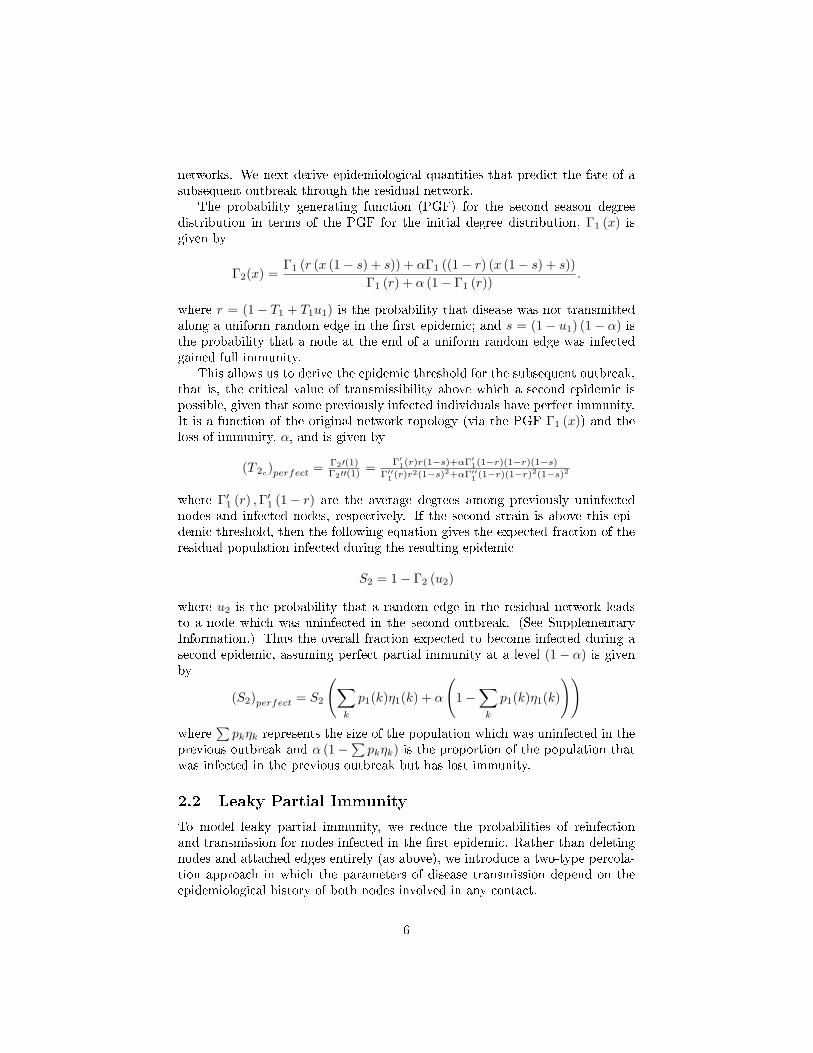
The probability generating function (PGF) for the second season degreedistribution in terms of the PGF for the initial degree distribution, Γ1 (x) isgiven by

Γ2(x) =Γ1 (r (x (1− s) + s)) + αΓ1 ((1− r) (x (1− s) + s))

Γ1 (r) + α (1− Γ1 (r)).

where r = (1− T1 + T1u1) is the probability that disease was not transmittedalong a uniform random edge in the �rst epidemic; and s = (1− u1) (1− α) isthe probability that a node at the end of a uniform random edge was infectedgained full immunity.

This allows us to derive the epidemic threshold for the subsequent outbreak,that is, the critical value of transmissibility above which a second epidemic ispossible, given that some previously infected individuals have perfect immunity.It is a function of the original network topology (via the PGF Γ1 (x)) and theloss of immunity, α, and is given by

(T 2c)perfect = Γ2′(1)Γ2′′(1) = Γ′

1(r)r(1−s)+αΓ′1(1−r)(1−r)(1−s)

Γ′′1 (r)r2(1−s)2+αΓ′′

1 (1−r)(1−r)2(1−s)2

where Γ′1 (r) ,Γ′1 (1− r) are the average degrees among previously uninfectednodes and infected nodes, respectively. If the second strain is above this epi-demic threshold, then the following equation gives the expected fraction of theresidual population infected during the resulting epidemic

S2 = 1− Γ2 (u2)

where u2 is the probability that a random edge in the residual network leadsto a node which was uninfected in the second outbreak. (See SupplementaryInformation.) Thus the overall fraction expected to become infected during asecond epidemic, assuming perfect partial immunity at a level (1− α) is givenby

(S2)perfect = S2

(∑k

p1(k)η1(k) + α

(1−

∑k

p1(k)η1(k)

))where

∑pkηk represents the size of the population which was uninfected in the

previous outbreak and α (1−∑pkηk) is the proportion of the population that

was infected in the previous outbreak but has lost immunity.

2.2 Leaky Partial Immunity

To model leaky partial immunity, we reduce the probabilities of reinfectionand transmission for nodes infected in the �rst epidemic. Rather than deletingnodes and attached edges entirely (as above), we introduce a two-type percola-tion approach in which the parameters of disease transmission depend on theepidemiological history of both nodes involved in any contact.

6

2.2.1 Two-type Percolation

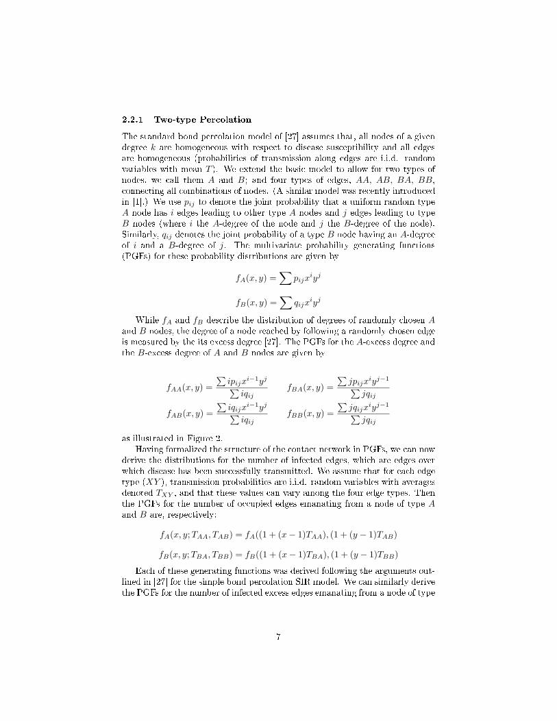
The standard bond percolation model of [27] assumes that, all nodes of a givendegree k are homogeneous with respect to disease susceptibility and all edgesare homogeneous (probabilities of transmission along edges are i.i.d. randomvariables with mean T ). We extend the basic model to allow for two types ofnodes, we call them A and B; and four types of edges, AA, AB, BA, BB,connecting all combinations of nodes. (A similar model was recently introducedin [1].) We use pij to denote the joint probability that a uniform random typeA node has i edges leading to other type A nodes and j edges leading to typeB nodes (where i the A-degree of the node and j the B-degree of the node).Similarly, qij denotes the joint probability of a type B node having an A-degreeof i and a B-degree of j. The multivariate probability generating functions(PGFs) for these probability distributions are given by

fA(x, y) =∑

pijxiyj

fB(x, y) =∑

qijxiyj

While fA and fB describe the distribution of degrees of randomly chosen Aand B nodes, the degree of a node reached by following a randomly chosen edgeis measured by the its excess degree [27]. The PGFs for the A-excess degree andthe B-excess degree of A and B nodes are given by

fAA(x, y) =∑ipijx

i−1yj∑iqij

fBA(x, y) =∑jpijx

iyj−1∑jqij

fAB(x, y) =∑iqijx

i−1yj∑iqij

fBB(x, y) =∑jqijx

iyj−1∑jqij

as illustrated in Figure 2.Having formalized the structure of the contact network in PGFs, we can now

derive the distributions for the number of infected edges, which are edges overwhich disease has been successfully transmitted. We assume that for each edgetype (XY ), transmission probabilities are i.i.d. random variables with averagesdenoted TXY , and that these values can vary among the four edge types. Thenthe PGFs for the number of occupied edges emanating from a node of type Aand B are, respectively:

fA(x, y;TAA, TAB) = fA((1 + (x− 1)TAA), (1 + (y − 1)TAB)

fB(x, y;TBA, TBB) = fB((1 + (x− 1)TBA), (1 + (y − 1)TBB)

Each of these generating functions was derived following the arguments out-lined in [27] for the simple bond percolation SIR model. We can similarly derivethe PGFs for the number of infected excess edges emanating from a node of type

7

A (B), at which we arrived by following a uniform random edge from a node oftype A (B):

fAA(x, y;TAA, TAB) = fAA((1 + (x− 1)TAA), (1 + (y − 1)TAB))

fBA(x, y;TAA, TAB) = fBA((1 + (x− 1)TAA), (1 + (y − 1)TAB))

fAB(x, y;TBA, TBB) = fAB((1 + (x− 1)TBA), (1 + (y − 1)TBB))

fBB(x, y;TBA, TBB) = fBB((1 + (x− 1)TBA), (1 + (y − 1)TBB))

The PGFs for outbreak sizes starting from a node of type A or B, respec-tively, are then given by

FA(x, y;TAA, TAB) = xfA(FAA(x, y; {T}), FAB(x, y; {T});TAA, TAB)

FB(x, y;TBA, TBB) = yfB(FBA(x, y; {T}), FBB(x, y; {T});TBA, TBB)

where, FAA and FBA are the PGFs for the outbreak size distribution startingfrom an (infected) node of type A which has been reached by following an edgefrom another (infected) node of type A or B, respectively. Similarly, FAB andFBB are the PGFs for the outbreak size distribution starting from an (infected)node of type B which has been reached by following an edge from another(infected) node of type A or B, respectively. These PGFs are as follows

FAA(x, y; {T}) = xfAA(FAA(x, y; {T}), FAB(x, y; {T});TAA, TAB)

FBA(x, y; {T}) = xfBA(FBA(x, y; {T}), FBB(x, y; {T});TAA, TAB)

FAB(x, y; {T}) = yfAB(FBA(x, y; {T}), FBB(x, y; {T});TBA, TBB)

FBB(x, y; {T}) = yfBB(FBA(x, y; {T}), FBB(x, y; {T});TBA, TBB)

Again following the method of [27], we can derive the expected size of a smalloutbreak and the epidemic threshold (given in the Supplementary Information).The expected numbers of A and B nodes infected in a small outbreak are foundby taking partial derivatives of the PGF for the outbreak size distribution:

〈s〉A =∂FA∂x|x=1,y=1 +

∂FB∂x|x=1,y=1

〈s〉B =∂FA∂y|x=1,y=1 +

∂FB∂y|x=1,y=1

Finally, we can �nd the size of a large-scale epidemic among A nodes andamong B nodes as:

SA (TAA, TAB) = 1−FA(1, 1;TAA, TAB) = 1−∑

pij(1+(a−1)TAA)i(1+(c−1)TAB)j

(2)

SB (TBA, TBB) = 1−FBB(1, 1;TBA, TBB) = 1−∑

qij(1+(b−1)TBA)i(1+(d−1)TBB)j

(3)

8

where, a = FAA(1, 1; {T}), b = FBA(1, 1; {T}), c = FAB(1, 1; {T}), d =FBB(1, 1; {T}). The probability of a large-scale epidemic can be derived sim-ilarly. The numerical values for the size and probability of an outbreak willbe equal if TAB = TBA. Further details are provided in the SupplementaryInformation.

This two-type percolation model provides a general framework for modelingpathogens with variable transmissibility and host populations with immunolog-ical heterogeneity.

2.2.2 Modeling Leaky Immunity with Two-Type Percolation

We now apply the two-type percolation method to model leaky partial immu-nity. In this model, type A nodes represent individuals who were not infected inthe initial epidemic and thus have no prior immunity, and type B nodes repre-sent those who were infected and maintain partial immunity (at a level 1− α).(Note that α gives the fraction of immunity lost in both models.) Here, we as-sume that prior immunity causes equal sized reductions in both infectivity andsusceptibility (α); but the approach can be extended easily to include more com-plex models of immunity. Speci�cally, during the subsequent epidemic, type Aindividuals (previously uninfected) have a susceptibility of one and an infectiv-ity of T2,while type B individuals (previously infected) have a susceptibility of αand an infectivity of T2α. Correspondingly, TAA = T2, TAB = T2α, TBA = T2α,and TBB = T2α

2 .The joint degree distributions for type A and type B nodes depend on the

course of the initial epidemic, and are given by

pij = p1(i+ j)η1(i+ j)(i+ ji

)ui1 (1− u1)j

qij = p1(i+ j) (1− η1(i+ j))(i+ ji

)ui1 (1− u1)j

respectively, where i is the A-degree and j is the B-degree. Further expla-nation can be found in Supplementary Information.

Using the quantities derived above, we can model epidemics that leave vary-ing levels of individual-level partial immunity. Using equations 2 and 3, forexample, we can solve for the size of the epidemic in a second epidemic with(individual-level) leaky partial immunity, (1− α):

(S2)leaky =

(∑k

p1(k)η1(k)

)SA (T2, T2α)+

(1−

∑k

p1(k)η1(k)

)SB(T2α, T2α

2).

9

3 Results

3.1 Impact of One Epidemic on the Next

We have introduced two distinct mathematical approaches for modeling theepidemiological consequences of naturally-acquired immunity. The residual net-work model probabilistically removes nodes and edges corresponding to thefraction (α) of infected nodes expected to lose immunity entirely. The two-type percolation model tracks the epidemiological history of all individuals andreduces the infectivity and susceptibility of all previously infected nodes by afraction (α). By adjusting α, both models can explore the entire range of im-munity from none to complete. At α = 1 , these model the absence or completeloss of immunity and thus would apply when the second season strain is entirelyantigenically distinct from the prior strain. At α = 0, these model full or noloss of prior immunity and might apply when a secondary epidemic is causedby the same or very similar pathogen as caused the �rst epidemic. Values of αbetween 0 and 1 represent partial immunity to the second pathogen, with thelevel of protection increasing as α approaches 0.

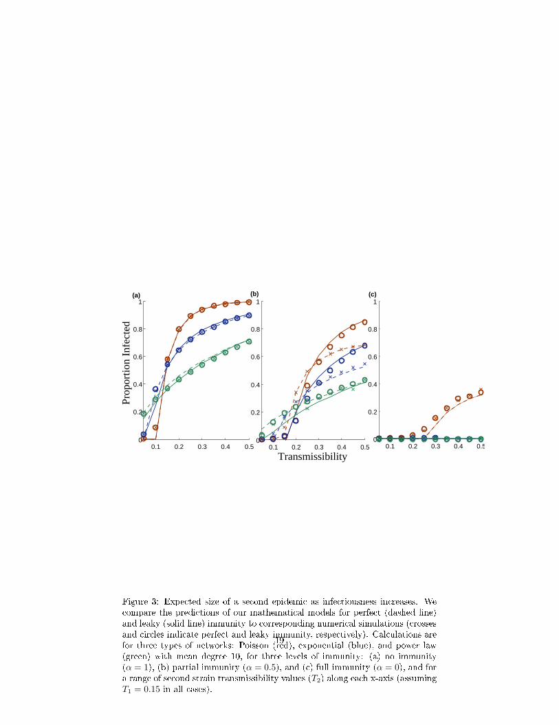
In Figure 3, we compare the predicted sizes of a second epidemic for boththe perfect and leaky models against simulations for a Poisson, exponential andscale-free random network (of the same mean degree) and under the conditionsof no prior immunity (α = 1), partial immunity (α = 0.5), and full immunity(α = 0) for values of transmissibility between 0 and 0.5 . There is a strongcongruence between our analytical calculations and their corresponding simu-lations. Assuming no immunity (Figure 3(a)), the two models simplify to thestandard bond percolation model on the original network, and thus make iden-tical predictions. Assuming full immunity (Figure 3(c)), the perfect immunitymodel removes all previously infected nodes (and the corresponding edges) be-fore the second outbreak; and the leaky immunity model sets transmissibilityalong all edges leading from and to previously infected nodes to zero, thus de-activating those nodes entirely. Consequently, the models also converge at thisextreme. The two models are, however, fundamentally di�erent for any levelof intermediate partial immunity between (0 < α < 1) as they assume di�erentmodels of immunological protection (Figure 3(b)). At α = 0.5, leaky immunityconfers greater herd immunity than perfect immunity at low values of transmis-sibility, while the reverse is true for more infectious pathogens. The makeupof the previously infected population is identical in both models and biased to-wards high degree individuals. When the pathogen is only mildly contagious,leaky immunity goes a long way towards protecting all previously infected hostswhereas perfect immunity protects only a fraction of these hosts; when it ismore highly contagious, however, leaky immunity is insu�cient to protect hostswith large numbers of contacts whereas perfect immunity is not diminished. We�nd further that network heterogeneity acts consistently across di�erent levelsof immunity. The Poisson network has the most homogeneous degree distribu-tion followed by the exponential network and �nally the scale-free network withconsiderable heterogeneity. Holding mean degree constant, variance in degree

10

increases the vulnerability of the population (allowing epidemics to occur atlower rates of transmissibility), yet generally reduces the ultimate size of epi-demics when they occur. At high levels of immunity, the susceptible networkat the start of the second season becomes more sparse and homogeneous. Thusthe impact of network variance on the second epidemic diminishes as immu-nity increases, that is, as α → 0. (We elaborate further on these results in theSupplementary Information.)

We explore intermediate levels of immunity further in Figure 4, and again�nd reasonable agreement between our analytic predictions and simulations. Asexpected, increasing levels of immunity (from left to right) decrease the epidemicpotential of a second outbreak.At these intermediate values of transmissibility(T1 = 0.15 and T2 = 0.3), leaky immunity tends to confer lower herd immunitythan perfect immunity, except at extremely high levels of immunity. The levelof immunity at which the predicted epidemic sizes for two immunity modelscross represents the point at which leaky partial immunity for all prior casese�ectively protects more individuals than the complete removal of a fraction ofthose cases. This transition point occurs at a higher level of immunity in theexponential network than the Poisson network, and never occurs in the scale-freenetwork, perhaps because the immunized individuals in the more heterogeneousnetworks tend to have anomalously high numbers of contacts thus limiting thee�cacy of partial protection.

3.2 Pathogen Re-invasion and Immune Escape

When a pathogen enters a population that has experienced a prior outbreak, itssuccess will depend on the extent and pattern of naturally-acquired immunityin the host population. The new pathogen may not be able to invade unless itis signi�cantly di�erent from the original strain. If it is antigenically distinctfrom the prior strain, then prior immunity may be irrelevant; and if it is moretransmissible than the original strain, then it may have the potential to reachpreviously unexposed individuals.

Figure 5 indicates the minimum transmissibility required for the new strainto cause an epidemic (that is, its critical transmissibility T2c

), as a function ofthe transmissibility of the original strain (T1) and the level of leaky immunity(α). The leakier the immunity (high α) and the lower the infectiousness of theoriginal strain (low T1), the more vulnerable the population to a second epidemic(light coloration in Figure 5). Generally the homogeneous Poisson network isless vulnerable to re-invasion than the heterogeneous scale-free network. Theblue curves in �gure 5 show combinations of T1 and α where the epidemicthreshold for the new strain equals the transmissibility of the original strain(T2c = T1) and have two complementary interpretations. First, if we assumethat the new strain is exactly as transmissible as the original strain (T = T2 =T1), then the curves indicate the critical level of cross-immunity (αc(T )) belowwhich the strain can never invade and above which the strain can invade withsome probability that increases with α. This threshold indicates the extentof antigenic evolution (or intrinsic decay in immune response) required for a

11

second epidemic to occur. The more heterogeneous the contact patterns (scale-free versus Poisson network), the lower the amount of immune escape requiredfor a pathogen of the same transmissibility to re-invade. Second, if we assumea �xed level of immune decay (α), then the curves indicate the critical initialtransmissibility (T1) above which the new strain can only invade if it is morecontagious than the original strain (T2 > T1). Below this point, the networktopology and preexisting immunity create a selective environment that excludesthe original strain and favors more transmissible variants. The perfect immunitymodel yields similar results (Supplementary Information.)

Some epidemiologists have speculated that there are 'trade-o�s' betweenvirulence and infectiousness, implying that more infectious pathogens will nec-essarily be more virulent [2, 14, 11, 17]. If true, �gure 5 suggests that naturally-acquired immunity, by opening niches for more infectious variants, may in-directly lead to the evolution of greater virulence. This is consistent with aprevious study showing that that host populations with high levels of immunitymaintain more virulent pathogens than naï¾÷ve host populations [18].

4 Discussion & Conclusion

In this work, we have considered the impact of pathogen spread on future out-breaks of the same or similar pathogen and on pathogen invasion and evolution.We have compared two standard models for immunity, perfect and leaky, andfound that the extent of herd immunity varies with the pathogen transmissibil-ity and the degree and nature of immunity. Leaky immunity appears to confergreater herd immunity at moderate levels of pathogen infectiousness for all lev-els of partial immunity, whereas perfect immunity is more e�ective at highertransmissibilities.

This analysis also has implications for public health intervention strategies.Contact-reducing interventions (e.g., patient quarantine and social distancing)and vaccination often result in complete removal of a fraction of individualsfrom the network (akin to perfect immunity), whereas transmission-reducinginterventions (e.g., face-masks and other hygienic precautions) typically reducetransmissibility along edges leading to and from a fraction of individuals (akinto leaky immunity) [32]. These results thus suggest that contact reductions willbe more e�ective than a comparable degree of transmission reductions at higherlevels of pathogen infectiousness.

The evolution of new antigenic characteristics in a pathogen that escape priorimmunity and the evolution of higher transmissibility both depend on geneticvariation. Thus, the more infections there are in the �rst season, the greater theopportunity for evolutionary change [6]. This poses a trade-o� for the pathogen:a large initial epidemic may generate variation that fuels evolution yet wipes outthe susceptible pool for the subsequent season; while a small initial outbreakleaves a large fraction of the network susceptible to future transmission yetmay fail to generate su�cient antigenic or other variation for future adaptation.We have shown that the trade-o� between generating immunity via infections

12

and escaping immunity via antigenic drift will depend not only on the sizeof the susceptible population, but also on its connectivity. Although we havefocused primarily on the role of antigenic drift, these models also apply to loss ofimmunity through decay in immunological memory, as occurs following pertussisand measles infections [26, 38].

Much epidemiological work, particularly the analysis of intervention strate-gies, ignores the immunological history of the host population. Thus our e�ort toincorporate host immune history into a �exible individual-based network modelwill potentially advance our understanding of the epidemiological and evolution-ary dynamics of partially-immunizing infections such as in�uenza, pertussis, orrotavirus. However, these provide just an initial step in this direction, as themodels consider only two consecutive seasons and do not yet allow for replen-ishment or depletion of susceptibles due to births and deaths.

Acknowledgments

This work was supported by the RAPIDD program of the Science & TechnologyDirectorate, Department of Homeland Security, and the Fogarty InternationalCenter, National Institutes of Health, and grants from the James F. McDonnellFoundation and National Science Foundation (DEB-0749097) to L.A.M.

References

[1] A. Allard, P. Noel, L. Dube, and B. Pourbohloul. Heterogeneous bond per-colation on multitype networks with an application to epidemic dynamics.Phys Rev E, 79 (3):036113, 2009.

[2] R. M. Anderson and R. M May. Coevolution of hosts and parasites. Para-sitology, 85:411�426, 1982.

[3] S. Bansal, M. Ferrari, and L.A. Meyers. The structural evolution of hostpopulations and the feedback on pathogens. In preparation.

[4] S. Bansal, B. Grenfell, and L.A. Meyers. When individual behavior matters.J. R. Soc. Interface, 4(16), 2007.

[5] A. Barbour and D. Mollison. Stochastic Processes in Epidemic Theory,chapter Epidemics and random graphs, pages 86�89. Springer, 1990.

[6] M. F. Boni, J. R. Gog, V. Andreasen, and F. B. Christiansen. In�uenza driftand epidemic size: the race between generating and escaping immunity.Theoretical population biology, 65(2):179�191, March 2004.

[7] M.F. Boni and M.W. Feldman. Evolution of antibiotic resistance by humanand bacterial niche construction. Evolution, 59 (3), 2005.

13

[8] M. Boots and A. Sasaki. Small worlds and the evolution of virulence. Proc.R. Soc. B, 266:1933�1938, 1999.

[9] C.O. Buckee, K. Koelle, M.J. Mustard, and S. Gupta. The e�ects ofhost contact network structure on pathogen diversity and strain structure.PNAS, 101 (29):10839�44, 2004.

[10] J. Bukh, R. Thimme, J. Meunier, K. Faulk, H. Spangenberg, K. Chang,W. Satter�eld, F. Chisari, and R. Purcell. Previously infected chimpanzeesare not consistently protected against reinfection or persistent infectionafter reexposure to the identical hepatitis c virus strain. Journal of Virology,82:8183�8195, 2008.

[11] J. Bull. Virulence. Evolution, 48:1423�35, 1994.

[12] S. Chaves, P. Gargiullo, J. Zhang, R. Civen, and D. et al Guris. Loss ofvaccine-induced immunity to varicella over time. NEJM, 356:1121�1129,2007.

[13] M.L. Clements, R.F. Betts, E.L. Tierney, and B.R. Murphy. Serum andnasal wash antibodies associated with resistance to experimental challengewith in�uenza a wild-type virus. J Clin Microbiol, 24:157�60, 1986.

[14] P.W Ewald. Transmission modes and evolution of the parasitism-mutualismcontinuum. Ann. NY Acad. Sci., 503:295�306, 1987.

[15] P. Farci, H. J. Alter, S. Govindarajan, D. C. Wong, R. Engle, R. R.Lesniewski, I. K. Mushahwar, S. M. Desai, R. H. Miller, N. Ogata, andR. H. Purcell. Lack of Protective Immunity Against Reinfection with Hep-atitis C Virus. Science, 258:135�140, October 1992.

[16] M. Ferrari, S. Bansal, L.A. Meyers, and O. Bjornstad. Network frailty andthe geometry of herd immunity. Proc. of R. Soc, 273:2743�2748, 2006.

[17] S.A. Frank. Models of parasite virulence. Q. Rev. Biol., 71:37�78, 1996.

[18] Sylvian Gandon, Margaret J. Mackinnon, Sean Nee, and Andrew F. Read.Imperfect vaccines and the evolution of pathogen virulence. Nature,414:751�756, 2001.

[19] N.C. Grassly, C. Fraser, and G.P. Garnett. Host immunity and synchro-nized epidemics of syphilis across the united states. Nature, 433:417�421,2005.

[20] R.E. Hope-Simpson. The transmission of epidemic in�uenza. PlenumPress, New York, 1992.

[21] F. Hoppenstead and P. Waltman. A problem in the theory of epidemics ii.Math Biosci, 12:133�145, 1971.

14

[22] S. Kaufmann, A. Sher, and R. Ahmed. Immunology of Infectious Diseases.ASM Press, 2002.

[23] W.O. Kermack and A.G. McKendrick. A contribution to the mathematicaltheory of epidemics. Proc. R. Soc. A, 115:700�721, 1927.

[24] S. Levin, J. Dusho�, and J. Plotkin. Evolution and persistence of in�uenzaa and other diseases. Math Biosci, 188:17�28, 2004.

[25] L.A. Meyers, B. Pourbohloul, M.E.J. Newman, D.M. Skowronski, and R.CBrunham. Network theory and sars: predicting outbreak diversity. J. Theo.Biol, 232:71�81, 2005.

[26] J. Mossong and C.P.clem Muller. Modelling measles re-emergence as aresult of waning of immunity in vaccinated populations. Vaccine, 21:4597�4603, 2003.

[27] M.E.J. Newman. Spread of epidemic disease on networks. Phys. Rev. E.,66(016128), 2002.

[28] A. Nunes, M.M. Telo da Gama, and M.G.M Gomes. Localized contactsbetween hosts reduce pathogen diversity. Journal of Theoretical Biology,241:477�87, 2006.

[29] M. Nuno, C. Castillo-Chavez, Z. Feng, and M. Martcheva. Lecture Notes

in Mathematics, chapter Mathematical Models of In�uenza: The Role ofCross-Immunity, Quarantine and Age-Structure, pages 349�364. SpringerBerlin, 2008.

[30] F.J. Odling-Smee, K.N. Laland, and M.W. Feldman. Niche construction:The neglected process in evolution. Monographs in Population Biology.,2003.

[31] R. Pastor-Satorras and Vespignani A. Epidemic dynamics and endemicstates in complex networks. Phys Rev E, 63(066117), 2001.

[32] B. Pourbohloul, L.A. Meyers, D.M. Skowronski, M. Krajden, and D.M.Patrick. Modeling control strategies of respiratory pathogens. Emerg Infect

Dis, 11:1249�1256, 2005.

[33] J. Read and M.J Keeling. Disease evolution on networks: the role of contactstructure. Proc R Soc B, 270:699�708, 2003.

[34] M. Recker, O. Pybus, S. Nee, and S. Gupta. The generation of in�uenzaoutbreaks by a network of host immune responses against a limited set ofantigenic types. PNAS, 104:7711�7716, 2007.

[35] M.D.F. Shirley and S.P Rushton. The impacts of network topology ondisease spread. Ecol. Complex, 2:287�299, 2005.

15

[36] J.L.0 Shulman. E�ects of immunity on transmission of in�uenza: Experi-mental studies. Progr. Med. Virol., 12:128�16, 1970.

[37] M. van Baalen. Adaptive Dynamics of Infectious Diseases: in Pursuit of

Virulence Management, chapter Contact networks and the evolution ofvirulence. Cambridge University Press, Cambridge, 2002.

[38] M. van Boven, H.E. de Melker, J.F. Schellekens, and M. Kretzschmar. Wan-ing immunity and sub-clinical infection in an epidemic model: implicationsfor pertussis in the netherlands. Mathematical Biosciences, 164:161�182,2000.

[39] P. Waltman. Deterministic threshold models in the theory of epidemics.Lecture Notes in Biomathematics, 1, 1974.

[40] D. Watts and S.H Strogatz. Collective dynamics of small world networks.Nature, 393(441), 1998.

[41] L. White, J. Buttery, B. Cooper, D. Nokes, and G. Medley. Rotaviruswithin day care centres in oxfordshire, uk: characterization of partial im-munity. J R Soc Interface, 5:1481�1490, 2008.

16

epidemic

Residual Contact Network

Leaky Partial ImmunityPerfect Partial Immunity

(a)

(c)(b)

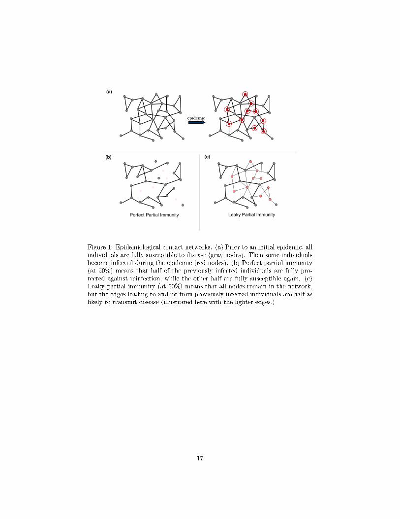
Figure 1: Epidemiological contact networks. (a) Prior to an initial epidemic, allindividuals are fully susceptible to disease (gray nodes). Then some individualsbecome infected during the epidemic (red nodes). (b) Perfect partial immunity(at 50%) means that half of the previously infected individuals are fully pro-tected against reinfection, while the other half are fully susceptible again. (c)Leaky partial immunity (at 50%) means that all nodes remain in the network,but the edges leading to and/or from previously infected individuals are half aslikely to transmit disease (illustrated here with the lighter edges.)

17

A A B B

A B A B

A B

AA B

BA

A B

BA

A B

BA

A B

B

AA B

BA

A B

B

fA(x,y) g

B(x,y)

gBB(x,y)g

AB(x,y) f

BA(x,y)f

AA(x,y)

Figure 2: The probability generating functions give the numbers of A and Bcontacts for each type of vertex (top). The four excess degree distributions givethe numbers of each type of contact for a vertex chosen by following a uniformrandom edge (bottom).

18

0.1 0.2 0.3 0.4 0.50

0.2

0.4

0.6

0.8

1

Prop

ortio

n In

fect

ed

0.1 0.2 0.3 0.4 0.50

0.2

0.4

0.6

0.8

1

Transmissibility

0.1 0.2 0.3 0.4 0.50

0.2

0.4

0.6

0.8

1(c)(b)(a)

Figure 3: Expected size of a second epidemic as infectiousness increases. Wecompare the predictions of our mathematical models for perfect (dashed line)and leaky (solid line) immunity to corresponding numerical simulations (crossesand circles indicate perfect and leaky immunity, respectively). Calculations arefor three types of networks: Poisson (red), exponential (blue), and power law(green) with mean degree 10, for three levels of immunity: (a) no immunity(α = 1), (b) partial immunity (α = 0.5), and (c) full immunity (α = 0), and fora range of second strain transmissibility values (T2) along each x-axis (assumingT1 = 0.15 in all cases).

19

00.510

0.2

0.4

0.6

0.8

1

Pro

port

ion

Infe

cted

00.510

0.2

0.4

0.6

0.8

1

α: No Immunity −−> Full Immunity00.51

0

0.2

0.4

0.6

0.8

1

(a) (b) (c)

Figure 4: Expected size of a second epidemic as immunity increases. We com-pare predictions of the perfect immunity model (gray dashed lines), leaky im-munity model (black solid lines) and simulations for each model (gray cross andblack circle markers, respectively). Calculations and simulations are for net-works with (a) Poisson, (b) exponential, and (c) scale-free degree distributionswith mean degree 10, at transmissibilities T1 = 0.15 and T2 = 0.3.

20

Lo

ss o

f Im

mu

nit

y (α

)

Transmissibility of first pathogen (T1)

0.2 0.3 0.4 0.5

0

0.5

1

0

0.1

0.2

0.3

0.4

0.5

0.6

0.7

0.8

0.9

1

0.1 0.2 0.3 0.4 0.5

0

0.5

1

Second epidemic likely

(a) (b)

T2

c

= T1

T2

c

= T1

T2

c

Second epidemic likely

Figure 5: Epidemic threshold (T2c) in the second season. The colors indicate

the level of transmissibility required for the second strain to invade the popu-lation (cause an epidemic), assuming leaky partial immunity for (a) a Poisson-distributed network and (b) a scale-free network, each with mean degree of 10.The x-axis gives the �rst season transmissibility (T1) and y-axis gives the lossof immunity (α). The blue line denotes T2c

= T1,: above the line T2c< T1, and

invasion by the original pathogen is possible.

21