The Impact of Mergers on the Degree of Competition in the Banking Industry

Impact of Mergers on the Degree of Competition: Application to the Banking Industry

Vittoria Cerasi†, Barbara Chizzolini‡ and Marc Ivaldi§

This draft: November 15, 2011

revised June 7, 2012

Abstract: This paper analyses the relation between competition and concentration in a monopolistic competition model where banks compete in branching and interest rates and market structure is endogenous. The model is applied on individual bank data in Italy and France using a maximum likelihood approach to derive a measure of the degree of competition in each local market. We propose an empirical test to evaluate ex-ante the impact of horizontal mergers on this measure. Depending on the pre-merger market structure and geographic distribution of branches, we find either cases where the merger is pro-competitive or anti-competitive. It proves its relevance as a tool for competition policy analysis. In addition, thanks to its theoretical foundation, it encompasses more information than traditional measures of competition while it is parsimonious in terms of data requirements. JEL classifications: G21 (Banks); L13 (Oligopoly); L59 (Regulation and industrial policy). Keywords: Banking industry; Competition and market structure; Merger policy. Acknowledgement: We thank Rosella Creatini, Wolf Wagner and Sub Ramanarayanan for helpful discussions and participants, among others Stijn Ferrari, Peter Davis, Thorsten Beck, Elu Von Thadden, Hans Degryse and Robert Marquez at the ACE Workshop on Antitrust and Regulation, Fondazione Eni Enrico Mattei, Milan (October 2009), the 2nd CEPR-EBC-UA Conference on competition in banking markets, Antwerp (December 2009) and the ZEW Conference on Quantitative Analysis in Competition Assessments, Mannheim (October 2010). Chizzolini acknowledges V. Chiorazzo and C. Milani at ABI for useful comments and for providing data on Italian banking groups and Ente L.Einaudi for financial support, while Cerasi acknowledges financial support from FAR 2008 and 2009 from Bicocca University. This paper was produced as part of the SCIFI-GLOW Collaborative Project supported by the European Commission’s Seventh Framework Programme for Research and Technological Development, under the Socio-economic Sciences and Humanities theme (Contract no. SSH7-CT-2008-217436). † Corresponding author: Department of Statistics, Bicocca University, Via Bicocca degli Arcimboldi 26, 20126 Milan (Italy), [email protected], phone: +39-02-6448.5821, fax. +39-02-6448.5878. ‡ Department of Economics, Bocconi University, via Roentgen 1, 20136 Milan (Italy), [email protected] § Toulouse School of Economics, University of Toulouse, 21, Allée de Brienne, 31000 Toulouse (France), [email protected].

‐ 2 ‐

Introduction

From a general perspective performing a comprehensive analysis of the relation

between competition and concentration in the banking industry is critical in view to evaluate

competition policies designed for this sector, as for instance the Second European Directive

implemented in 1992. It is well admitted that, while this directive has instantaneously restored

competition among banks after years of tight regulatory constraints, it has also indirectly

prompted a wave of mergers within national borders. As a result, the degree of concentration,

measured in terms of market shares, has risen in almost all European countries. Since

deregulation was aimed at promoting competition, this rise in concentration raises the concern

that the reverse objective obtains.

How do we measure the degree of competition in a market and what is its relation with

concentration? It is well documented that the relation between competition and concentration

cannot be reduced to the view that they are inversely related, as stated by the structure-

conduct-performance (SCP) paradigm promoted by Bain (1956). As a matter of fact, when

taking into account the changes in market structure, the relation may be reversed: Firms tend

to exit competitive industries in the anticipation that profits will be lower than entry costs.

This explains why tougher price competition may be followed by an increase in the degree of

concentration, hence delivering a positive relation that contrasts with the SCP paradigm.

From a more specific perspective, the antitrust investigation of single cases of

proposed mergers between dominant firms calls for an assessment of their likely impact on

competition. To what extent a merger provides the new entity with the ability to raise prices at

the detriment of consumers and rivals and creates the conditions favouring coordinated

behaviour among firms is at the core of the merger policy. The literature provides contrasting

evidence on the impact of mergers on competition in the banking system as discussed in

Degryse and Ongena (2008) and Carletti and Vives (2009). In the short term, when the

involved banks gain efficiency, due to economies of scale and scope, and pass on the benefits

to consumers by reducing prices of banking products, competition is enhanced; however

when merged banks exploit their greater market power in order to increase prices, rivalry may

be reduced. (See Sapienza, 2002, for a discussion of these contrasting effects.) In the longer

term, however changes in the incentive to enter or exit the industry may further affect

competition and an empirical analysis is required to be able to assess the overall impact of

mergers (as for instance in Focarelli and Panetta, 2003). When analysing the impact of

‐ 3 ‐

mergers among incumbent banks it is therefore crucial to rely on a model where competition

and market structure are simultaneously determined.

This paper proposes a measure of the degree of competition1 for the banking industry

originated from a model where entry is endogenous. The proposed measure is obtained from

the econometric estimation of a monopolistic competition model, where banks compete in

retail markets by setting interest rates and branches, and captures the ability of banks to

translate an enlargement of their branching network into higher profits. A tougher rivalry in

interest rates reduces this ability, thus revealing greater competition. This measure is affected

by the structure of the local market, in particular by the dispersion of market shares and the

number of large players in the market, together with other standard measures of concentration

such as the Herfindahl–Hirschman Index (HHI, herein).

Our econometric model is exploited here to evaluate the impact of a merger on this

proposed measure of competition. Indeed, after having obtained the branching network of the

merged bank by summing the pre-merger networks, we can re-estimate the model in order to

derive the new measure of competition. By comparing the pre- and post-merger measures of

competition, we exhibit examples of mergers that are pro-competitive, even though the

merger causes an obvious increase in concentration in market shares. This may occur when

the asymmetry between market shares falls or when the number of large banks competing at

the top in each local market rises as a result of mergers between mid-size players.

Our measure of competition is based on a parsimonious quantity of information since

basically it only requires a measure of the size of local markets and data on branching market

shares of individual banks in these local markets, without any knowledge of accounting data -

even when publicly available - at this level of disaggregation. These are the same

informational requirements used to compute the HHI, which is the measure of concentration

commonly used in the antitrust analysis.

Our approach is not specific to banks as it can be easily exported to other retail

industries which require a network to distribute their products and services, as for instance in

insurance, grocery stores, car dealers, or in industries where firms enter with one branch such

as doctors or lawyers.

This paper is related to the empirical literature in industrial organization based on

game theoretical models with endogenous market structure inspired by Sutton (1991). We

1 In the sequel, we often simplify the term “the measure of the degree of competition” in “the measure of competition.”

‐ 4 ‐

depart from the SCP paradigm by empirically investigating the relation between competition

and concentration along the line of an approach initiated by Bresnahan and Reiss (1991a,

1991b), more recently re-examined by Berry and Tamer (2006), based on models of firms

entry and in an application to product differentiated industries by Schaumans and Verboven

(2011).

Their basic idea is that, by observing the presence of a firm in a market, it is possible

to recover information about profits and sunk costs of entry as the decision to enter reveals

that profits are larger than entry costs; otherwise the firm would have not entered. We thus

apply the same logic to the choice of branching: By its presence in a market with a given

number of branches, a bank reveals that it expects to recover the cost of a branching network

of that size. Then we can derive information about the non-observable cost of branching by

observing the branch presence in a market. In this literature there is a potential problem of

identification: Profits and sunk costs are in fact estimated up to a monotonic transformation.

We have solved it here by introducing a measure of competition that only affects profits

without affecting branching costs. In this way we are able to estimate directly a measure of

the degree of competition. Our paper exploits further this result to study the changes in

market structure following a merger to measure the changes in the degree of competition.

Our results show that the impact of mergers cannot be fully captured by measuring the

change in market concentration only: When for instance the market structure is fragmented

with a single dominant firm, a horizontal merger between medium-size players might restore

competitive conditions by generating a rival for the dominant firm in the market. In this case,

greater concentration in market shares is accompanied by greater competition, breaking down

the inverse relation between concentration and competition. (See also Cetorelli, 1999, and

Berger et al., 2004.)

The paper is based on preliminary articles where we consider, as the reference

markets, respectively the Italian provinces between 1989 and 1995 in Cerasi et al. (2000) and

the national industry for several European countries before and after the implementation of

the Second European Directive in 1992 in Cerasi et al. (2002). Here we apply the same

methodology for individual banks using local markets –namely “département” for France and

“provincia” for Italy- as the reference markets between 2004 and 2007. We are here able to

compare two countries on the same basis, i.e., with the same model and similar reference

markets on data of higher quality. However the main novelty here is the use of the model to

evaluate the effect of a merger on the average degree of competition in the industry. More

‐ 5 ‐

specifically we study the effect of mergers in France, among which that of Crédit Agricole

with Crédit Lyonnais, and the two most important mergers in the latest years in Italy, namely

Intesa with San Paolo IMI and Unicredito with Capitalia. We find mergers with opposite

effects on competition, pro-competitive in France, while anti-competitive in Italy. Their

opposite impact is explained by the differences in the pre-merger structure of local markets, in

particular in terms of dispersion of market shares and number of large banks in the market.

More specifically, this paper is related to studies measuring competition in retail

markets using structural models of monopolistic competition. In a recent paper Schaumans

and Verboven (2011) estimate a measure of change in competition within a model of product

differentiated industries and apply it to local services markets. They estimate the ordered

probit entry model, as in Bresnahan and Reiss (1991a, 1991b), jointly with an industry

revenue function to obtain a competition measure that adds to the estimated change in per-

firm profits due to new entry a new component linked to the elasticity of demand to new

entry. Their approach is close in its objective to our cci measure, but it imposes heavier data

requirements compared to our test. This is why we think it cannot be easily adapted to

industries characterized by a large number of firms or branches as in our case.

Based on the idea that firms in more competitive markets suffer a larger loss in profits

when their costs increase, Boone (2008) and Boone et al. (2007) propose a measure of

competition that coincides with the elasticity of profits to costs. We use a similar idea by

proposing a measure of competition that captures the ability of banks to translate an increase

in their branching network into profits, that is the elasticity of profits to branching: In contrast

to the other papers however, our measure of competition does not require any knowledge of

accounting data. Cohen and Mazzeo (2007) propose a model of monopolistic competition in

branching to estimate the competitive response of banks. Our approach is similar, since we

both estimate directly the structural equations in order to infer non-observable entry costs;

however we move further in exploiting the model to simulate the impact on competition of

horizontal mergers.

The exercise of simulation of mergers based on a structural model of monopolistic

competition contrasts with other papers in the literature where the impact measurement is

carried ex post on accounting data after banking mergers have occurred. (See the applications

to the banking industry in Molnar, 2008, and Zhou, 2008.) In those papers the exercise

consists in estimating demand and supply parameters before the mergers and then, using them

to simulate a change in the ownership allocation of branches with the purpose of assessing

‐ 6 ‐

their impact on competition (as surveyed in Budzinski and Ruhmer, 2008). Our objective is to

derive an impact assessment before the merger occurs, without imposing heavy data

requirements other than the information to compute the HHI at local market level. We believe

that our method provides a useful guide to competition authorities to assess ex-ante the impact

mergers.

In Section 1 we derive the econometric test from a theoretical model of bank

branching behaviour and propose a measure of the degree of competition in local markets.

The results of the econometric test applied to individual bank data in local markets in France

and Italy are presented in Section 2. Section 3 is devoted to the evaluation of the ex ante

impact of specific horizontal mergers on the degree of competition using our econometric

model, while Section 4 discusses the relation between our estimated measure of competition

and concentration in market shares. Finally Section 5 concludes the paper.

1. Definition and measure of the degree of competition

We first define the degree of competition within a reduced-form model of

monopolistic competition where branching is a strategic competitive tool for banks in local

markets.2 Then we derive an econometric model to obtain an estimate of this measure of

competition in the banking industry.

1.1. The model

In our model, banks compete on interest rates, given their choice of entry and

branching in a specific local market.3 Each bank enters a local market whenever its expected

profits are large enough to recover entry costs and expands its branching network up to the

point where marginal benefits equate marginal costs. We assume that banks instantaneously

adjust their branching networks to the optimal size in each period and market. Box 1 provides

2 Branching is important in retail markets since geographic proximity still represents a competitive advantage when monitoring opaque SMEs or when supplying current accounts, as argued in Petersen and Rajan (2002), Degryse and Ongena (2005), and Brevoort ans Hannan (2006). 3 The model presented in this paper is a reduced form of a two stage model: in the first stage each bank decides to enter and the size of its branching network, while in the second stage it competes in interest rates. See Cerasi (1996) for the full characterization of the model.

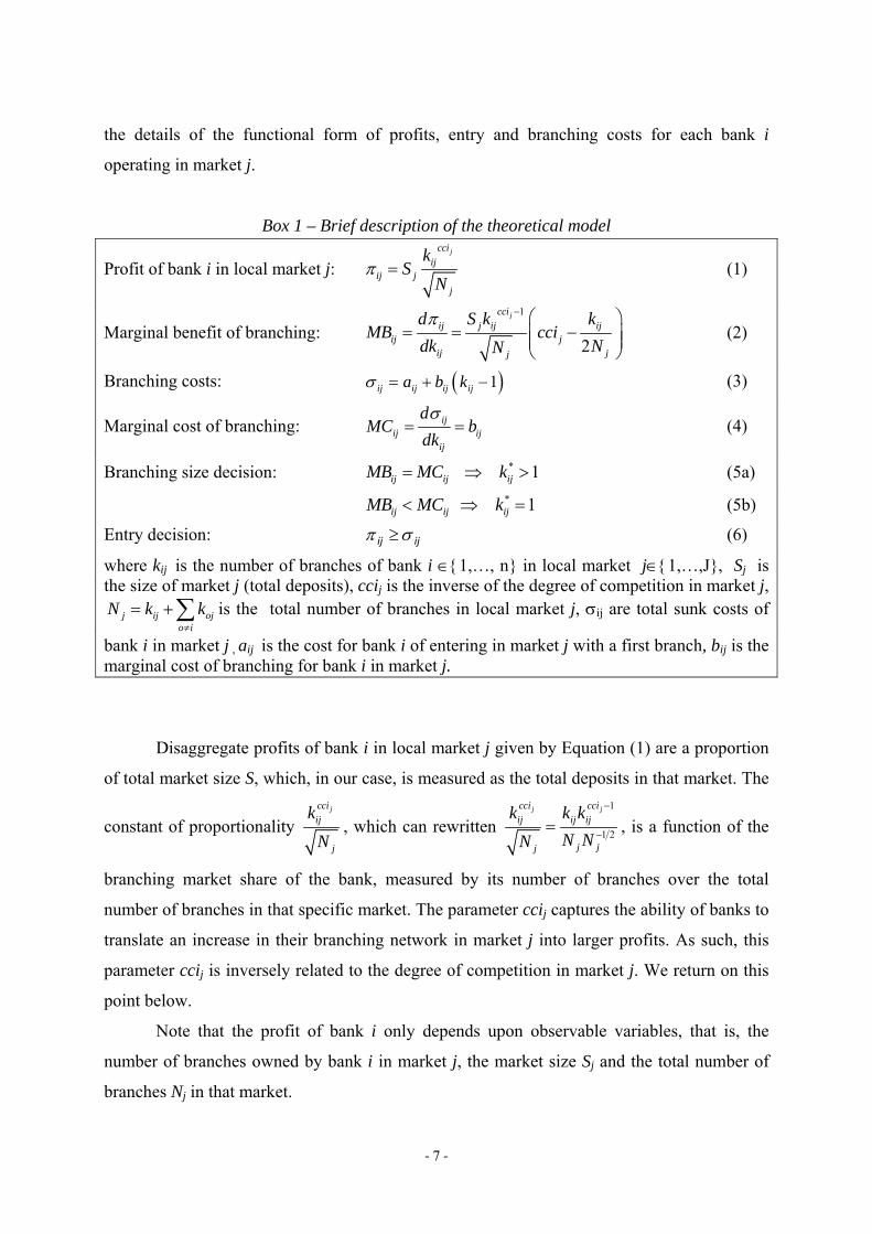
‐ 7 ‐

the details of the functional form of profits, entry and branching costs for each bank i

operating in market j.

Box 1 – Brief description of the theoretical model

Profit of bank i in local market j: jcci

ijij j

j

kS

N (1)

Marginal benefit of branching: 1

2

jcci

ij j ij ijij j

ij jj

d S k kMB cci

dk NN

(2)

Branching costs: 1ij ij ij ija b k (3)

Marginal cost of branching: ijij ij

ij

dMC b

dk

(4)

Branching size decision: * 1ij ij ijMB MC k (5a)

* 1ij ij ijMB MC k (5b)

Entry decision: ijij (6)

where kij is the number of branches of bank i 1,…, n in local market j1,…,J, Sj is the size of market j (total deposits), ccij is the inverse of the degree of competition in market j,

j ij ojo i

N k k

is the total number of branches in local market j, ij are total sunk costs of

bank i in market j , aij is the cost for bank i of entering in market j with a first branch, bij is the marginal cost of branching for bank i in market j.

Disaggregate profits of bank i in local market j given by Equation (1) are a proportion

of total market size S, which, in our case, is measured as the total deposits in that market. The

constant of proportionality jcci

ij

j

k

N, which can rewritten

1

1 2

j jcci cci

ij ij ij

j jj

k k k

N NN

, is a function of the

branching market share of the bank, measured by its number of branches over the total

number of branches in that specific market. The parameter ccij captures the ability of banks to

translate an increase in their branching network in market j into larger profits. As such, this

parameter ccij is inversely related to the degree of competition in market j. We return on this

point below.

Note that the profit of bank i only depends upon observable variables, that is, the

number of branches owned by bank i in market j, the market size Sj and the total number of

branches Nj in that market.

‐ 8 ‐

By using this specification, we are imposing several properties to the profit function.

First, per-bank profit increases with total market size Sj since a fixed number of banks in a

larger market manage to share greater revenues. Second, per-bank profit decreases with the

overall number of branches in the market Nj: As the market becomes further crowded with

branches, per-bank profit shrinks. Third, per-bank profit increases with own branches kij at a

rate given by the parameter ccij according to Equation (2): The more intense is the

competition in interest rates in a given market, the smaller the per-bank profit and marginal

gain of opening a new branch. This is why our parameter measures, although indirectly,

competition in interest rates in market j through its effect on the elasticity of profits to

branching.4 If competition in interest rates becomes tougher then the additional gain from

opening a new branch decreases. Hence a smaller ccij captures greater competition in market

j.

The optimal branching size is achieved when its marginal benefits equates its marginal

costs of branching. From Equation (3), branching costs are linear in kij and therefore the

marginal cost bij in Equation (4), is constant. Each bank sets its branching network size at

* 1ijk , according to Equation (5a) by equating the marginal benefit of an additional branch to

the marginal cost; otherwise * 1ijk if Equation (5b) holds.

Dropping the subscripts, for given S and N, the optimal branching size increases with

cci and decreases with marginal branching cost. For a given market size and number of

competitors, if competition in the market becomes tougher (lower cci) the bank may end up

closing branches ( *k will decrease) since the expected gains from a larger branching network

shrink.

We may explain the choice of the optimal branching size with a numerical example. In

Figure 1 we draw the constant marginal cost and marginal benefits as functions of k, given by

Equations (2) and (4), for the values: S=6000, N-k=300, b=75. The dashed line represents the

marginal cost MC, while the continuous line MB is the marginal benefit when cci is 0.9. The

optimal branching size is given by the intersection between MB and MC in A at * 380k

4 The parameter cci is defined as ln

ln 2

k

k N

, which represents the elasticity of profits to an additional branch

whenever k/2N becomes negligible. Notice that the value cci in principle could change with the number of banks in the market, as indeed one might expect from a measure of competition. However as N becomes large relatively to k, it becomes independent.

‐ 9 ‐

approximately. If competition becomes tougher, that is when cci falls from 0.9 to 0.8, then

MB shifts on the left (dotted line) so that the intersection is now reached in B and the optimal

branching size shrinks to *' 100k . Clearly in our model, a tougher price competition has

ceteris paribus a negative impact on branching size.

Figure 1 – Optimal branching size

A final component of the model is the free entry condition which requires banks to

enter a market only if their expected profits are greater than entry costs for given branching

size, as stated by Equation (6). Note that we can estimate the sunk costs as soon as we have an

estimate of marginal costs.

1.2. The econometric model

To recover branching costs from observed choices of branching, we follow an

approach initiated by Bresnahan and Reiss (1991 a, 1991b) and reinvigorated by Berry and

Tamer (2006). Now we explain how to achieve this objective starting from the model

presented in the previous section.

0

40

80

1200 1600 2000 0

100

200

300

‐ 10 ‐

In equilibrium either one of two branching Conditions (5a) and (5b) must hold, since

banks adjust their branching networks to the optimal size in each period and local market. As

the data allows us to observe the change in the number of branches from one year to the other,

we may exploit this additional information in the econometric model in order to retrieve the

non-observable branching costs. We classify each observation, namely a bank i in period t

and in local market j, according to either of the following four categories:

[a] “expanding multi-branch” bank if kijt= (kijtkijt-1) > 0 and kijt >1;

[b] “static multi-branch” bank if kijt= 0 and kijt >1;

[c] “shrinking multi-branch” bank if kijt < 0 and kijt >1;

[d] “unit-branch bank if kijt= 0 and kijt =1.

Notice that for multi-branch banks concerned by cases [a] to [c], Condition (5a) must hold,

while for unit-branch banks in [d], Condition (5a) is replaced by Condition (5b).

Now we substitute the definition of MBijt in the branching Conditions (5a) and (5b)

with the following quantity

1

2

jtcci

jt ijt ijtijt jt

jtjt

S k kA cci

NN, (7)

where, instead of the number of branches at time t, we use its lagged value kijt-1 inside the

brackets. Notice that Aijt>MBijt when kijt> 0, while Aijt<MBijt when kijt < 0. Then we can

say that for any bank in [a] it must be that Aijt>MBijt , for banks in [b] and [d] it is Aijt=MBijt ,

while for banks in [c] it is Aijt<MBijt .

Finally, with respect to Conditions (5a) and (5b), we simplify the partitioning of all

observations into two sub-sets:5

1

2

: all banks in [a] and [b] so that

: all banks in [c] and [d] so that

ijtt ijt

t ijt ijt

E A MC

E A MC (8)

The econometric test requires casting each observation into the probability space.

Therefore we must make assumptions on the stochastic component of the model, that is to

say, the non-observable branching cost. We assume that it is idiosyncratic, independent and

5 Notice that we have made an arbitrary choice when choosing to classify the “static multi-branch” banks in the sub-set E1t. We check the robustness of our results due to this classification criterion in the next section.

‐ 11 ‐

with known probability distribution. More specifically, we assume that the logarithm of the

marginal cost is specified as:

ln ijt ijt ijtMC mc v , (9)

where mcijt is the deterministic component and ijt is the stochastic term with standard normal

distribution Φ(.).

According to the partitioning of observations defined by Equation (8) and our

stochastic assumptions, the probability that each observation falls either in the subset E1t

(expanding or static multi-branch banks) or in E2t (shrinking multi-branch or unit-branch

banks) is given by:

1

2

Pr ( ) Pr Pr ln ln

Pr ( ) Pr Pr ln 1 ln

t ijt ijt ijt ijt ijt ijt ijt

t ijt ijt ijt ijt ijt ijt ijt

ij E MC A v A mc A mc

ij E MC A v A mc A mc (10)

Then the likelihood function for all observations in the dataset is obtained as

tt Eij

ijtijt

Eij

ijtijt mcAmcAL

21

ln1lnlnlnln (11)

The parameters ccijt and mcijt are identifiable and estimated by maximizing the likelihood

function. We further assume that the inverse measure of competition ccijt and the marginal

costs mcijt are specified as linear function of the market and bank specific variables Wjt and Zijt

respectively.

2.Empiricalanalysis

In this section we measure the degree of competition in each local market based on the

estimated values of the parameter cci from the econometric specification of the previous

section. After a brief description of the dataset, we present the results.

2.1. The data

In the econometric model, the reduced form of profits, the marginal branching benefit

and in particular the threshold value Aijt, are all functions of observable variables either

market specific variables such as the market size Sjt measured by the total amount of deposits,

‐ 12 ‐

and the total number of branches Njt in the market, or bank specific variables such as the

number of branches of bank i in market j at time t, kijt, and its lagged value kijt-1.

Note that our analysis does not require any knowledge of accounting data. As a matter

of fact disaggregated accounting measures of per-bank profit are not even available at the

local level: accounting sources provide uniquely consolidated balance sheet data, that is,

aggregate across all markets in which the bank operates. For instance, suppose that bank A

owns branches in market a and b: From its accounting statements we would be able to recover

only consolidated profits across the two markets, not the two separate profits, i.e. the profit of

bank A in market a and profit of bank A in market b, as required by the analysis of the

competitive behavior of banks at local level. Our theoretical model however provides a simple

proxy for the profits on each market, as expressed by the reduced form given in Equation (1),

which is a function of the market share of the bank in each local market computed in terms of

the number of branches.

Our local markets are the 95 départements in France and the 103 provinces in Italy.

Note that many brand-name banks share the same ownership. We assume that banks

belonging to the same group tend to coordinate their decisions in terms of interest rates and

branching. Thus groups and not banks should be the most appropriate unit of observation.6

Each observation is therefore a banking group i operating in local market j at time t with

given branching size ijtk .7

We recovered the information on the number of branches for each individual banking

group in each local market for 2005 and 2007 in France, and for 2004 and 2006 in Italy. We

therefore have a cross-section for each country which allows us to compute ijtk , i.e., the

change in branching size for each group in each local market, taking 2005 (resp. 2004) as the

initial year for France (resp. Italy).

6 We consider that, on the one hand, smaller groups or independent banks have no strategic behavior as they are price takers and are marginally adapting their branching behavior. They are nevertheless included in the denominator Nj, representing the total number of branches in that market, since they nevertheless exert a competitive pressure on branches of the main groups in each local market behaving like a fringe. On the other hand, we include La Poste among banks in France as the banking part of the French postal mail provider has a large and dispersed network. In contrast, Poste Italiane is excluded as it did not play a similar role at the time of our analysis. 7 To capture coordination among banks belonging to the same group across different local markets in our econometric analysis, we control for ownership by using a dummy variable specific to each group.

‐ 13 ‐

For Italy, data on bank branches by “provincia” are taken from the public site of Bank

of Italy.8 For France data on bank branches by “départements” were provided directly by

Crédit Agricole and Caisses d’Epargne. In France all banks have branches in each of the 95

departments, with the only exception of C.I.C. that has no branches in Corsica. In Italy six

national banks have branches located in almost all 103 provinces, while the remaining groups

have their branching networks geographically concentrated in few local markets. Descriptive

statistics in Table 1 show that the two industries are similar only for what concerns the

dispersion of branches within markets, measured by the standard deviation. We observe

across markets smaller average and median branching sizes for Italy, implying that there are

larger groups in France. The number of total branches in each market is larger in France, that

is, there are several large players simultaneously in each market.

[Insert Table 1 here]

Our definition of bank’s profits in each local market must be highly correlated with

bank accounting profits, not available at this level of disaggregation. In support to this, we

know that accounting profits are proportional to market shares in terms of deposits and, since

these are highly correlated with branching market shares, we expect high correlation also

between reduced profits computed in our model and observed accounting profits.

In the empirical specification for mci, we include the dummies to identify banking

groups in the set of explanatory variables Zit. The inverse measure of competition cci instead

depends upon a set of market variables, Wjt, which comprises per-capita loans (LPC), the

proportion of rural areas in each county (SHRUR) and a dummy indicating densely populated

urban areas (DBIGPRO). These variables are taken from the Central Statistical Offices,

INSEE for France and ISTAT for Italy. We expect to find tougher competition the higher per-

capita loans and population density due to greater incentive to compete for the marginal client

when demand is larger.

8 The data on branches for individual banks are taken from www.bancaditalia.it, while we have followed the ABI guidelines for the definition of banking groups.

‐ 14 ‐

2.2 Econometric results

The parameter cci is estimated for 2006 in Italy and 2007 in France on cross-sections

that we call the base models. All coefficients that result from the maximum likelihood

estimation in Table 2 are significant, although their value is variable across markets capturing

local differences. The signs of the coefficients associated to cci are in accordance with our

intuition: in France in those Départments where there is a greater share of rural areas

(SHRUR) banks face softer competition and, similarly, in Italy competition is tougher in

those provinces where a big city is located (DBIGPRO). In addition, in both countries the

degree of competition increases with the level of per-capita loans (LPC).


A measure of the performance of the model in fitting the data, defined as “goodness of

fit”, is obtained by comparing the predicted to the actual partitioning of observations between

subset E1 (all expanding multi-branch or static multi-branch banks) and E2 (all shrinking

multi-branch or unit-branch banks). Table 3 reports the percentage of observations whose

behavior in terms of branching is correctly predicted by the model: this percentage is 84% for

France and 75% for Italy.9


Table 4 provides evidence that the two industries differ in terms of competition,

branching costs and profitability. The average value of cci, is higher in Italy, 1.17, compared

to France, 0.68 (recall that lower values of cci imply tougher competition) indicating that

local markets are on average more competitive in France than in Italy. Note that marginal

costs are lower in France compared to Italy and moreover, represent a smaller share of our

estimated per-branch profits: the French bank system is not only more competitive but more

efficient.


Table 5 exhibits heterogeneity of estimated marginal branching costs across banking

groups, in particular Crédit Agricole and La Poste have higher costs and considerably lower

per-branch profits compared to the other French groups. These two groups are indeed

characterized by large branching networks with branches distributed all over the country, even

9 To check the robustness of our partitioning we have re-estimated the model moving the static multi-branch banks (case [b] in sub-section 1.2) from subset E1 to subset E2 defined in Equation (8). Under this partitioning the percentage of observations correctly classified decreases significantly.

‐ 15 ‐

in less densely populated areas. In Italy instead, per-branch profits are relatively

homogeneous across banking groups, with higher marginal costs for Unicredito. The

heterogeneity of marginal costs across banking groups is smaller in Italy compared to France.


In Tables 9a and 9b (in Appendix), we report a ranking of local markets based on our

estimated measure of competition. As already observed the parameter cci varies considerably

across local markets. In densely populated areas our measure cci takes smaller values

indicating tougher competition. For instance in Paris cci assumes its smallest value. In Italy

the overall variance of cci is greater. Notice that cci takes lower values in several Italian

Northern provinces compared to Southern provinces. This result suggests that banks located

in Northern regions face greater competition compared to those located in Southern regions,

confirming previous empirical evidence. (See Cerasi et al., 2000 and Guiso et al., 2006,

among others.)

3.Impactmeasurementofmergersoncompetition

We now use the econometric model to simulate the ex-ante impact of mergers on

competition. For each merger, we undertake the following exercise: we sum the branches of

the merging banks in each local market and re-estimate the model assuming that these new

entities replace the old ones, without changing the distribution of branches across local

markets. It yields the estimated post-merger degree of competition, which we compare to the

pre-merger degree of competition (estimated from the actual situation). We expect that this

measure provides a useful guide to competition authorities to assess the impact of banks’

mergers on competition. However we recognize that our measure, which requires a very

limited amount of information, cannot fully anticipate how rival banks adapt their branching

networks after a merger as we keep as given the total number of branches.10

10 There is an empirical literature providing evidence that the anti-competitive impact of a merger may be considerably affected by the competitive reaction of non-merged firms and new entries in the market. (See for instance the discussion in Draganska et al., 2009.)

‐ 16 ‐

3.1 French mergers

Two among the most important mergers really occurred in France in the recent years,

that is Credit Mutuel (CM) with Credit Industriel Commercial (CIC) in 1998 and Crédit

Agricole (CA) with Crédit Lyonnais (CL) in 2004. Given that our French dataset includes the

number of branches for each merger as separate banking group even after the merger, we can

exploit this information to retrieve the pre-merger situation (which corresponds to our

estimated base model) and simulate the impact of the merger “as if” the merger occurred in

our observation period.

Table 6 reports the comparison of the relevant indicators between the base model and

the model with the merger. The result of this exercise shows that these two mergers together

improve competition in the industry. Table 9a (in Appendix) displays the impact of the two

mergers in each single local market: the differences in the estimated values of the cci are

significant and negative.


A further exercise is to add the merger between Banques Populaires (BP) and Caisses

d’Epargne (CE), approved after 2007 to the previous simulation. Also in this case the

parameter cci decreases compared to the base model (see last row in Table 6 for France). This

result proves that the initial pro-competitive effect of the merger still remains.11

3.2 Italian mergers

A similar exercise can be performed for the two most relevant Italian mergers in the

recent years, namely Intesa (IN) with San Paolo (SP) and Unicredito (UN) with Capitalia

(CP). Notice that in our observed period the exercise is “virtual” since the merger actually

occurred at the end of 2007. In Table 6 we summarize the changes of the main indicators as a

result of the two mergers.

The two mergers have an anti-competitive effect, as it results from the increase in the

estimated value of cci with respect to the base model (last row in Table 6 for Italy). The

differences in the two measures of competition are significant as Table 9b (in Appendix)

shows.

11 See Ivaldi (2006) for a detailed analysis of this merger, available upon request.

‐ 17 ‐

The difference between the impact of these mergers compared to the French case can

be better interpreted by analyzing their effect on the local market structure, as we do in the

last section.

4.Concentrationandcompetition

In this section we first investigate the relation between our measure of competition and

the usual measures of concentration at local market level, namely, the Herfindahl–Hirschman

Index (HHI), the GINI index and the number of large undertakings in each local market. The

idea behind these traditional measures is that, when market shares are uniformly distributed,

the market power is more balanced among firms and, as a consequence, competition is

greater. Indeed, the HHI is the sum of squared market shares and captures the degree of

concentration in branching at local market level: this index gives more weight to changes in

market shares of largest banks since large banks have greater shares. The GINI index

measures the distance between the actual distribution and the case of uniform market shares:

this index increases with the inequality between market shares. Finally we compute the

number of banks with a market share above the average (N. large banks), in each specific

market. 12

What we would like to explore is whether our measure of degree of competition is

similar to these usual concentration measures or conveys additional and more accurate

information. To do so, we compute the correlations between our and the traditional measures

at local market level. The results in Table 7 show that these correlations are not null, meaning

that our degree of competition is indeed related to market structure as it falls with the HHI

and it increases with the number of large banks in the market. For the GINI index, we observe

that the correlation has opposite effects in the two countries: greater equality in the

distribution of market shares increases competition in France, but not in Italy.


12 The role of a large number of big players in enhancing competition is documented for instance by the debate

around the proposal of mergers in the Canadian banking industry. Using Bank of Canada’s words in response to Minister of Finance (23 June 2003): “In a given market, one player with a 45% market share can leave room for an acceptable level of competition, as long as there are two or three additional players with a certain critical mass who are also operating in the same market.”

‐ 18 ‐

Note that none of these traditional measures in isolation captures the degree of

competition in a market, because they only focus on the supply side of the market, while we

consider also the demand side when we measure the elasticity of profits to the number of

branches through our index cci.

To understand the impact of mergers on competition we analyze how they affect

market structure at the local level. Table 8 shows that the two mergers of CA with CL and

CM with CIC in France have a pro-competitive effect, since the average cci across

Departments falls from 0.68 to 0.54. Although the two mergers generate two large banking

groups in France, we observe a reduction in the Gini index from 0.57 to 0.53 and a rise in the

number of banks with a market share above the average from 2.71 to 3.06. Notice that even

though concentration rises as measured by the HHI due to the increase in the market shares of

the top largest banks, according to our measure of the degree of competition the two French

mergers promote competition. This positive impact on competition can be explained by the

fact that they reduce the asymmetry in the distribution of market shares. The merger between

CA and CL, two large players with complementary branching networks, and the merger

between two medium players such as CM with CIC, increase the presence of several large

banks in all Departments and this benefits competition.


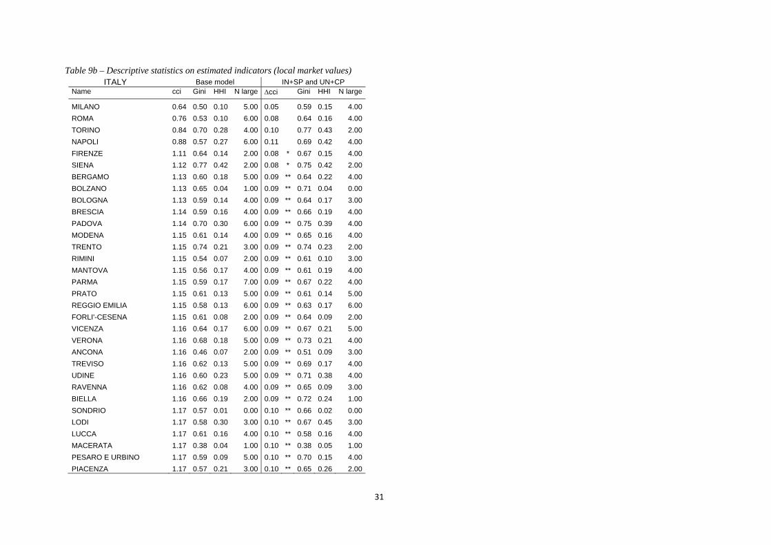
In Italy instead, the mergers of IN with SP and UN with CP have a negative impact on

competition, as evident from the increase in the value of cci across provinces from 1.17 to

1.27. In contrast with the French exercise, in Italy the asymmetry between market shares rises

following the mergers; the Gini index rises from 0.58 to 0.63, the number of large banks

declines from 3.59 to 3.16 and the HHI rises from 1900 to 2400. The impact of the two Italian

mergers is clearly anti-competitive at local market level: they in fact take place among the top

players in the market and the overall effect is a reinforcement of their previous strong local

market power.

Our econometric test shows how it would be misleading to base the impact assessment

of a merger only on the change in the degree of concentration as it used to be in merger policy

before the reforms in Europe and in the U.S, which have limited the use of the dominance

criteria as the sole test in merger assessment13. In our simulation for instance, this rule would

13 See Shapiro (2010) and Gilbert and Rubinfield (2011) for reviews of merger guidelines in U.S. and E.U before the reforms. They both argue how pre-reform guidelines emphasized the stand-alone role of pre and post-merger HHI thresholds to challenge a merger.

‐ 19 ‐

imply rejecting the French mergers, while we have shown their role in enhancing competition.

At the same time, note that the data required to implement our measure is similar to those

required to compute local market concentration indexes such as the HHI.

Conclusion

This paper addresses the question of how to measure the impact of mergers on

competition in the banking sector. This question is relevant both from a positive and a

normative point of view.

We provide a measure of competition in retail banking markets, derived from a model

where branching decisions are modelled together with market structure. This measure is based

on the elasticity of profits with respect to branching: the smaller the elasticity the higher the

degree of competition. Our evidence indicates that the retail banking industry in France is

more competitive than in Italy.

In addition we propose an empirical test to be used in the antitrust analysis for the ex-

ante impact assessment of mergers on competition. This test is parsimonious in terms of data

requirements and is grounded on a theoretical model where competition is analysed together

with market structure. In our simulated examples we exhibit either cases of pro- and anti-

competitive mergers.

Our findings are based on a static model where banks choose their optimal branching

size in each period. It is part of our future research agenda to take into account a more

dynamic version of the branching competition game. (See Chizzolini, 2011, for preliminary

results.)

References

Bain J.S.,1956, Barriers to New Competition, Harvard University Press. Berger A., Demirgüç-Kunt A., Levine R., Haubrich J., 2004, Bank Concentration and

Competition: An Evolution in the Making, Journal of Money Credit and Banking, 36 (3), 433-451

Berry S., and Tamer E., 2006, Identification in Models of Oligopoly Entry, in R.Blundell, W. Newey, T. Persson (eds.) Advances in Economics and Econometrics, Econometric Society Monographs.

‐ 20 ‐

Boone J., 2008, A New Way to Measure Competition, Economic Journal, 118, 1245-1261. Boone J., C van Ours J., and van der Wiel H., 2007, How (not) to Measure Competition,

CEPR Discussion Paper N.6275. Brevoort K., and Hannan T., 2006, Commercial Lending and Distance: Evidence from

Community Reinvestment Act Data, Journal of Money, Credit and Banking, 38(8), 1991-2012.

Bresnahan, T., and P. Reiss, 1991a, Empirical Models of Discrete Games, Journal of Econometrics, 48, 57-81.

Bresnahan, T., and P. Reiss, 1991b, Entry and Competition in Concentrated Markets, Journal of Political Economy, 99, 977–1009.

Budzinski O., Ruhmer I., 2009, Merger Simulation in Competition Policy: A Survey, Available at SSRN: http://ssrn.com/abstract=1138682

Carletti E. and Vives X., 2009, Regulation and Competition Policy in the Banking Sector, in X. Vives (ed.), Competition Policy in Europe, Fifty Years of the Treaty of Rome, Oxford University Press, 260-282.

Cerasi V., 1996, A model of Retail Banking Competition, unpublished manuscript, Università degli Studi di Milano.

Cerasi V., Chizzolini B, and M. Ivaldi, 2000, Branching, and Competitiveness across Regions in the Italian Banking Industry, in Polo M. (ed.) Industria bancaria e concorrenza, Il Mulino, 499-522.

Cerasi V., Chizzolini B, and M. Ivaldi, 2002, Branching and Competition in the European Banking Industry, Applied Economics, 34, 2213-2225.

Cetorelli N., 1999, Competitive Analysis in Banking: Appraisal of the Methodologies, Economic Perspectives, Federal Reserve Bank of Chicago, Q1, 2-15.

Chizzolini B., 2011, A Multi-Period Model of Competition in Retail Banking, Rivista Bancaria, Minerva Bancaria N.3/2011.

Cohen A., Mazzeo M., 2007, Market Structure and Competition Among Retail Depository Institutions, Review of Economics and Statistics, 89 (1), 60-74.

Degryse H., Ongena S., 2005, Distance, Lending Relationship and Competition, Journal of Finance, 60(1), 231-266.

Degryse H., Ongena S., 2008, Competition and Regulation in the Banking Sector: A Review of the Empirical Evidence on the Sources of Bank Rents, in Thakor A. and A. Boot (eds.), Handbook of Financial Intermediation and Banking, Elsevier, 483-554.

Draganska M., Mazzeo M., Seim K., 2009, Addressing Endogenous Product Choice in an Empirical Analysis of Merger Effects, mimeo, Graduate School of Business, Stanford University.

Focarelli D., Panetta F., 2003, Are Mergers Beneficial to Consumers? Evidence from the Market for Bank Deposits, American Economic Review, 93(4), 1152-1172.

Gilbert R., Rubinfeld D., 2011, Revising the Horizontal Merger Guidelines: Lessons from the E.U. and the U.S., in Faure M., Zhang X. (eds.), Competition Policy and Regulations: Recent Developments in China, Europe and the U.S., Edward Elgar. Available at SSRN: http://ssrn.com/abstract=1660638.

Guiso L., Sapienza P., Zingales L., 2006, The Cost of Banking Regulation, CEPR Discussion Paper 5864.

Ivaldi M., 2006, Evaluation économique des effets d’une coordination éventuelle des groupes Banque Populaire et Caisse d’Epargne dans la banque de détail, Université de Toulouse, Juin.

Molnar J., 2008, Market Power and Merger Simulation in Retail Banking, Bank of Finland Research Discussion Papers N.4.

‐ 21 ‐

Petersen M.A. and Rajan R., 2002, Does Distance Still Matter? The Information Revolution in Small Business Lending, Journal of Finance, 57(6), 2533-2570.

Sapienza P., 2002, The Effects of Banking Mergers an Loan Contracts, Journal of Finance, 57(1), 329-367.

Schaumans C., Verboven F., 2011, Entry and Competition in Differentiated Products Markets, CEPR Discussion Paper No. 8353.

Shapiro C., 2010, The 2010 Horizontal Merger Guidelines: From Hedgehog to Fox in Forty Years. Available at SSRN: http://ssrn.com/abstract=1675210.

Sutton J., 1991, Sunk Costs and Market structure, MIT Press. Zhou X., 2008, Estimation of the Impact of Mergers in the Banking Industry, mimeo

Department of Economics Yale University.

Appendix – Tables

Table 1- Descriptive statistics on observable variables (local market values; for France in 2006, for Italy in 2007)

FRANCE

Total deposits

(S)

Total branches

(N)

Individual branches

(k)

Market share (k/N)

ITALY

Total deposits

(S)

Total branches

(N)

Individual branches

(k)

Market share (k/N)

Mean 12406.1 441 46 10.61 Mean 7064.2 237 19 7.89

Median 8091.4 373 23 5.36 Median 3647.6 163 7 4.10

Maximum 171591.3 1485 389 69.13 Maximum 128132.5 2050 435 83.04

Minimum 1691.1 91 0 0.00 Minimum 442.8 25 1 0.13

Standard deviation 18837.0 253 55 12.61 Standard deviation 15323.6 273 34 10.02 Note: Total deposits are expressed in Euro. Note: Total deposits are expressed in Euro.

23

Table 2 – Base model (maximum likelihood estimation)

FRANCE Coefficient P-value ITALY Coefficient P-value

cci

Constant 0.662 0.000

cci

Constant 1.243 0.000

SHRUR 0.082 0.192 DBIGPRO -0.340 0.000

LPC -0.003 0.000 LPC -0.003 0.000

mc Bank dummies mc Bank dummies

Log likelihood -346.0

Log likelihood -649.284

# obs 862 # obs 1226

% correct predictions* 84.1 % correct predictions* 75.4Note: SHRUR is the share of rural areas within a county, LPC are loans per-capita.

Note: DBIGPRO is a dummy indicating densely populated urban areas, LPC are loans per-capita.

* % correct predictions is derived by summing the percentages along the diagonal in Table 3.

Table 3 – Goodness of fit (comparison of predicted vs. actual observations in % )

FRANCE Predicted ITALY Predicted

Actual dk<0,k=1 dk≥0,k>1 Actual dk<0,k=1 dk≥0,k>1

dk<0,k=1 9.74 12.99 22.74 dk<0,k=1 5.22 19.58 24.8

dk≥0,k>1 2.9 74.36 77.26 dk≥0,k>1 5.06 70.15 75.2

12.65 87.35 100 10.28 89.72 100

24

Table 4 – Descriptive statistics on estimated values (local market values)

FRANCE cci MC Per-branch

profit ITALY cci MC

Per-branch profit

Mean 0.68 42.67 149.49 Mean 1.17 242.51 400.06

Median 0.69 39.20 115.99 Median 1.19 216.90 297.03

Maximum 0.71 99.38 2240.58 Maximum 1.23 502.23 2829.97

Minimum 0.32 22.45 18.20 Minimum 0.64 132.89 88.55

Standard deviation 0.04 22.71 208.34 Standard deviation 0.10 100.22 393.54

25

Table 5 – Descriptive statistics on estimated values(banking group values)

FRANCE MC Per-branch

profit N. branches

ITALY MC

Per-branch profit

N. branches

BANQUE NATIONAL DE PARIS 28.83 166.15 2154 BANCA ANTONIANA - POPOLARE 254.5 387.52 1007

BANQUES POPULAIRES 22.45 150.95 2475 BANCA INTESA 150.99 369.59 3029

CREDIT AGRICOLE 51.62 112.67 6238 BANCA LOMBARDA E PIEMONTESE 254.5 474.63 787

CAISSES D’EPARGNE 44.78 125.46 4312 BANCA NAZIONALE DEL LAVORO 132.89 366.86 731

CREDIT INDUSTRIEL COMMERCIAL 39.20 186.97 1692 BANCA POPOLARE DI LODI 194.68 400.37 901

CREDIT LYONNAIS 25.75 173.11 1947 BANCA POPOLARE DI VICENZA 254.5 446.76 524

CREDIT MUTUEL 48.96 182.56 3111 BANCA POPOLARE EMILIA ROMAGNA 254.5 410.12 1175

LA POSTE 99.38 81.86 15581 BANCHE POPOLARI UNITE (IN FORMAZIONE) 216.9 427.57 1205

SOCIETE GENERALE 23.02 166.43 2204 BANCO POPOLARE DI VERONA 254.5 450.27 1221

Mean 42,67 149,57 4412,67 BIPIEMME 446.58 540.84 713

Standard deviation 24,04 35,58 4429,78 CAPITALIA 200.53 371.07 2013

CARIGE 254.5 422.8 508

CREDITO EMILIANO - CREDEM 319.15 417.31 470

MONTE DEI PASCHI DI SIENA 168.11 369.94 1908

SANPAOLO IMI 178.57 371.02 3171

UNICREDITO ITALIANO 502.23 373.24 3028

Mean 252,35 412,49 1399,44

Standard deviation 99,67 48,15 942,40

26

Table 6- Changes in the estimated values as a result of mergers

FRANCE cci MC ITALY cci MC

Base model 0.68 42.67

Base model 1.17 242.51

CA+CL and CM+CIC 0.54 18.45 IN+SP and

UN+CP 1.27 335.54

CA+CL and CM+CIC and CE+BP 0.55 19.08 Note: IN=Intesa, SP=San Paolo IMI, UN=Unicredito,

CP= Capitalia Note: CA=Credit Agricole, CL=Credit Lyonnais, CM=Credit Mutuel, CIC= Crédit Industriel Commercial, CE=Caisses d'Epargne, BP=Banques Populaires

Table 7- Correlation between competition and measures of market structure

FRANCE cci HHI GINI N. Large

banks ITALY cci HHI GINI N. Large

Banks

cci 1.00 0.54 0.59 -0.49 cci 1 0.11 -0.07 -0.21 HHI 0.54 1.00 0.93 -0.72 HHI 0.11 1.00 0.53 -0.01 GINI 0.59 0.93 1.00 -0.70 GINI -0.07 0.53 1.00 -0.20 N. Large banks -0.49 -0.72 -0.70 1.00 N. Large banks -0.21 -0.01 -0.20 1.00

27

Table 8 – Impact of mergers on the inverse measures of competition and measures of market structure

FRANCE cci Gini HHI N. large banks

ITALY cci Gini HHI N. large banks

Base model 0.68 0.57 2400 2.71

Base model 1.17 0.58 1900 3.59 (0.04) (0.12) (0.08) (0.90) (0.09) (0.09) (0.11) (1.51)

CA+CL and CM+CIC 0.54 0.53 2600 3.06

IN+SP and UN+CP 1.27 0.63 2400 3.16 (0.03) (0.12) (0.08) (0.82) (0.09) (0.09) (0.14) (1.17)

CA+CL and CM+CIC and CE+BP 0.55 0.50 2700 3.48 Note: standard deviations are in brackets.

IN=Intesa, SP=San Paolo IMI, UN=Unicredito, CP= Capitalia. (0.03) (0.14) (0.08) (0.71)

Note: standard deviations are in brackets. CA=Credit Agricole, CL=Credit Lyonnais, CM=Credit Mutuel, CIC= Crédit Industriel Commercial, CE=Caisses d'Epargne, BP=Banques Populaires.

28

Table 9a – Descriptive statistics on estimated indicators (local market values) FRANCE Base model CA+CL and CM+CIC CA+CL and CM+CIC and CE+BP

Name cci Gini HHI N_large cci Gini HHI N_large cci Gini HHI N_large

Paris 0.32 0.29 0.07 5 -0.03 0.24 0.10 4 -0.01 0.13 0.11 5

Hauts-de-Seine 0.51 0.29 0.10 5 -0.07 0.24 0.13 4 -0.06 0.17 0.14 5

Val-de-Marne 0.63 0.29 0.10 6 -0.10 0.21 0.13 5 -0.09 0.18 0.14 5

Bouches-du-Rhône 0.64 0.37 0.12 4 -0.11 0.34 0.15 3 -0.10 0.30 0.16 3

Seine-Saint-Denis 0.64 0.34 0.11 5 -0.10 0.23 0.13 4 -0.09 0.20 0.15 5

Bas-Rhin 0.64 0.53 0.20 2 -0.13 * 0.51 0.24 3 -0.12 0.49 0.25 4

Haute-Savoie 0.65 0.47 0.16 2 -0.13 * 0.39 0.19 3 -0.12 0.36 0.20 4

Rhône 0.65 0.34 0.13 3 -0.13 * 0.33 0.16 4 -0.12 0.30 0.18 4

Marne 0.66 0.54 0.22 3 -0.14 * 0.52 0.25 3 -0.13 0.49 0.26 3

Haut-Rhin 0.66 0.56 0.22 2 -0.13 * 0.53 0.25 3 -0.12 0.52 0.27 4

Essonne 0.66 0.31 0.14 4 -0.12 0.26 0.16 5 -0.11 0.27 0.18 5

Nord 0.66 0.41 0.14 4 -0.12 0.33 0.18 5 -0.12 0.27 0.19 5

Loire-Atlantique 0.66 0.43 0.16 3 -0.13 * 0.41 0.19 3 -0.12 0.36 0.21 4

Yvelines 0.66 0.34 0.13 4 -0.13 * 0.26 0.15 5 -0.12 0.26 0.17 5

Ille-et-Vilaine 0.67 0.51 0.18 3 -0.14 * 0.43 0.21 3 -0.13 0.38 0.22 4

Territoire de Belfort 0.67 0.49 0.18 3 -0.13 * 0.46 0.21 3 -0.12 0.43 0.22 4

Seine-et-Marne 0.67 0.42 0.18 3 -0.13 * 0.38 0.20 4 -0.13 0.34 0.21 5

Finistère 0.67 0.55 0.19 3 -0.13 * 0.51 0.21 3 -0.13 0.46 0.22 4

Loiret 0.67 0.45 0.17 3 -0.14 * 0.44 0.20 4 -0.13 0.42 0.21 4

Gironde 0.67 0.45 0.18 4 -0.13 * 0.41 0.19 4 -0.13 0.40 0.21 4

Val-d'Oise 0.67 0.39 0.15 5 -0.13 0.34 0.17 5 -0.12 0.31 0.19 5

Vendée 0.67 0.62 0.23 3 -0.14 * 0.57 0.25 3 -0.13 0.52 0.25 3

Var 0.67 0.45 0.16 3 -0.13 * 0.41 0.18 3 -0.12 0.39 0.19 3

Hérault 0.68 0.56 0.18 4 -0.14 * 0.49 0.19 3 -0.13 0.48 0.20 3

Haute-Garonne 0.68 0.40 0.15 3 -0.14 * 0.32 0.17 3 -0.13 * 0.34 0.20 3

Morbihan 0.68 0.55 0.20 3 -0.14 * 0.49 0.22 3 -0.13 * 0.44 0.23 4

Moselle 0.68 0.51 0.20 3 -0.14 * 0.50 0.23 4 -0.13 * 0.48 0.25 4

Maine-et-Loire 0.68 0.60 0.23 3 -0.14 * 0.54 0.25 3 -0.13 * 0.49 0.26 4

Isère 0.68 0.50 0.20 3 -0.14 * 0.44 0.22 3 -0.13 * 0.43 0.24 3

Doubs 0.68 0.54 0.23 2 -0.14 * 0.51 0.25 3 -0.14 * 0.49 0.26 4

Vaucluse 0.68 0.55 0.17 4 -0.13 * 0.50 0.19 3 -0.13 0.47 0.20 3

Côte-d'Or 0.68 0.54 0.22 4 -0.14 * 0.50 0.24 4 -0.14 * 0.47 0.25 4

29


Alpes-Maritimes 0.68 0.38 0.13 4 -0.14 * 0.35 0.16 4 -0.13 * 0.34 0.17 4

Pyrénées-Orientales 0.68 0.62 0.24 3 -0.14 * 0.56 0.26 3 -0.13 * 0.56 0.28 3

Mayenne 0.68 0.67 0.27 3 -0.14 * 0.61 0.28 3 -0.14 * 0.56 0.29 3

Gard 0.68 0.63 0.25 3 -0.14 * 0.57 0.26 3 -0.13 0.56 0.27 3

Meurthe-et-Moselle 0.68 0.44 0.20 3 -0.14 * 0.46 0.23 4 -0.13 * 0.41 0.24 4

Indre-et-Loire 0.68 0.58 0.26 3 -0.14 * 0.55 0.28 3 -0.13 * 0.55 0.29 3

Savoie 0.68 0.63 0.22 3 -0.14 * 0.56 0.23 2 -0.13 * 0.56 0.24 3

Côtes d'Armor 0.68 0.66 0.26 3 -0.14 * 0.57 0.27 3 -0.14 * 0.53 0.27 3

Pyrénées-Atlantiques 0.68 0.48 0.15 4 -0.14 * 0.43 0.18 3 -0.13 * 0.42 0.19 3

Aveyron 0.68 0.69 0.34 3 -0.14 * 0.66 0.35 3 -0.14 * 0.65 0.36 3

Deux-Sèvres 0.69 0.58 0.22 4 -0.14 * 0.52 0.24 4 -0.14 * 0.48 0.25 4

Loire 0.69 0.48 0.19 3 -0.14 * 0.46 0.22 3 -0.13 * 0.44 0.23 3

Charente-Maritime 0.69 0.58 0.24 2 -0.14 * 0.55 0.25 3 -0.14 * 0.53 0.26 4

Vosges 0.69 0.51 0.22 3 -0.14 * 0.46 0.23 4 -0.13 * 0.43 0.25 4

Calvados 0.69 0.48 0.20 2 -0.14 * 0.47 0.22 3 -0.14 * 0.40 0.23 4

Seine-Maritime 0.69 0.43 0.16 3 -0.14 * 0.40 0.18 4 -0.14 * 0.34 0.19 4

Oise 0.69 0.54 0.21 3 -0.14 * 0.49 0.23 3 -0.13 * 0.44 0.24 3

Sarthe 0.69 0.57 0.24 4 -0.14 * 0.55 0.26 4 -0.14 * 0.49 0.27 4

Ain 0.69 0.58 0.25 2 -0.14 * 0.56 0.27 3 -0.14 * 0.53 0.28 4

Aube 0.69 0.57 0.25 2 -0.15 * 0.51 0.27 2 -0.14 * 0.52 0.28 3

Pas-de-Calais 0.69 0.54 0.19 3 -0.14 * 0.46 0.21 4 -0.13 0.39 0.22 4

Tarn 0.69 0.58 0.22 4 -0.14 * 0.51 0.24 4 -0.14 * 0.50 0.26 3

Haute-Vienne 0.69 0.66 0.28 3 -0.14 * 0.56 0.29 3 -0.14 * 0.55 0.31 3

Landes 0.69 0.62 0.26 2 -0.14 * 0.58 0.28 2 -0.14 * 0.57 0.29 3

Drôme 0.69 0.57 0.24 3 -0.14 * 0.55 0.25 3 -0.14 * 0.53 0.27 3

Lot-et-Garonne 0.69 0.66 0.28 2 -0.14 * 0.61 0.29 2 -0.14 * 0.60 0.31 3

Tarn-et-Garonne 0.69 0.67 0.31 2 -0.14 * 0.61 0.32 2 -0.14 * 0.60 0.33 3

Manche 0.69 0.53 0.20 4 -0.14 * 0.49 0.22 4 -0.14 * 0.43 0.23 4

Puy-de-Dôme 0.69 0.64 0.26 2 -0.14 * 0.58 0.29 2 -0.14 * 0.57 0.30 3

Eure-et-Loir 0.69 0.54 0.20 4 -0.14 * 0.49 0.22 4 -0.14 * 0.43 0.23 4

Loir-et-Cher 0.69 0.63 0.29 2 -0.14 * 0.61 0.30 2 -0.14 * 0.58 0.31 3

Vienne 0.69 0.65 0.29 3 -0.14 * 0.61 0.31 3 -0.14 * 0.60 0.31 3

Charente 0.69 0.64 0.31 2 -0.15 * 0.61 0.33 2 -0.14 * 0.58 0.33 3

Jura 0.70 0.61 0.28 3 -0.15 * 0.56 0.29 4 -0.14 * 0.58 0.31 4

30


Somme 0.70 0.65 0.25 3 -0.14 * 0.57 0.27 3 -0.14 * 0.50 0.27 3

Aude 0.70 0.76 0.41 2 -0.15 * 0.72 0.41 2 -0.14 * 0.71 0.42 3

Orne 0.70 0.58 0.22 3 -0.15 * 0.52 0.24 3 -0.14 * 0.47 0.25 4

Hautes-Alpes 0.70 0.73 0.34 2 -0.15 * 0.68 0.35 2 -0.14 * 0.67 0.36 3

Gers 0.70 0.70 0.30 2 -0.15 * 0.65 0.32 2 -0.14 * 0.64 0.33 3

Cantal 0.70 0.77 0.38 2 -0.15 * 0.72 0.39 2 -0.14 * 0.71 0.40 3

Aisne 0.70 0.62 0.27 3 -0.14 * 0.57 0.28 3 -0.14 * 0.52 0.29 3

Corrèze 0.70 0.73 0.34 2 -0.15 * 0.66 0.35 2 -0.14 * 0.66 0.36 3

Saône-et-Loire 0.70 0.57 0.26 3 -0.15 * 0.54 0.28 3 -0.14 * 0.52 0.29 3

Eure 0.70 0.52 0.21 3 -0.14 * 0.49 0.23 3 -0.14 * 0.43 0.24 3

Haute-Loire 0.70 0.69 0.29 3 -0.15 * 0.64 0.30 3 -0.14 * 0.61 0.31 3

Indre 0.70 0.70 0.31 3 -0.15 * 0.64 0.32 3 -0.14 * 0.62 0.33 3

Cher 0.70 0.67 0.28 2 -0.15 * 0.64 0.29 2 -0.14 * 0.63 0.30 3

Yonne 0.70 0.65 0.30 3 -0.15 * 0.61 0.31 3 -0.14 * 0.61 0.32 3

Haute-Saône 0.70 0.66 0.35 2 -0.15 * 0.65 0.36 3 -0.14 * 0.63 0.37 4

Allier 0.70 0.65 0.30 3 -0.15 * 0.59 0.31 3 -0.14 * 0.58 0.33 3

Lozère 0.70 0.76 0.40 2 -0.15 * 0.74 0.41 2 -0.14 * 0.73 0.42 3

Ardennes 0.70 0.62 0.27 2 -0.15 * 0.61 0.30 3 -0.14 * 0.56 0.30 4

Lot 0.70 0.69 0.31 3 -0.15 * 0.66 0.33 3 -0.14 * 0.65 0.35 3

Corse A 0.70 0.74 0.45 1 -0.15 * 0.74 0.46 2 -0.14 * 0.73 0.46 2

Nièvre 0.70 0.69 0.32 3 -0.15 * 0.65 0.33 3 -0.14 * 0.64 0.34 3

Hautes-Pyrénées 0.70 0.62 0.28 2 -0.15 * 0.58 0.30 2 -0.14 * 0.58 0.31 3

Dordogne 0.71 0.75 0.38 2 -0.15 * 0.69 0.38 2 -0.14 * 0.68 0.39 2

Meuse 0.71 0.72 0.38 2 -0.15 * 0.71 0.39 2 -0.14 * 0.69 0.40 3

Ariège 0.71 0.72 0.39 2 -0.15 * 0.68 0.40 2 -0.14 * 0.67 0.41 3

Ardèche 0.71 0.69 0.33 3 -0.15 * 0.68 0.35 3 -0.14 * 0.65 0.35 3

Corse B 0.71 0.78 0.50 1 -0.15 * 0.77 0.50 2 -0.14 * 0.75 0.51 2

Haute-Marne 0.71 0.72 0.40 2 -0.15 * 0.69 0.41 2 -0.14 * 0.67 0.41 3

Alpes-haute-Provence 0.71 0.71 0.33 2 -0.15 * 0.67 0.34 2 -0.14 * 0.66 0.35 3

Creuse 0.71 0.74 0.39 2 -0.15 * 0.71 0.40 2 -0.15 * 0.69 0.41 3Note: Difference in cci relative to base model significant at 10% level (*) or at 5% level (**).

31

Table 9b – Descriptive statistics on estimated indicators (local market values) ITALY Base model IN+SP and UN+CP

Name cci Gini HHI N large cci Gini HHI N large

MILANO 0.64 0.50 0.10 5.00 0.05 0.59 0.15 4.00

ROMA 0.76 0.53 0.10 6.00 0.08 0.64 0.16 4.00

TORINO 0.84 0.70 0.28 4.00 0.10 0.77 0.43 2.00

NAPOLI 0.88 0.57 0.27 6.00 0.11 0.69 0.42 4.00

FIRENZE 1.11 0.64 0.14 2.00 0.08 * 0.67 0.15 4.00

SIENA 1.12 0.77 0.42 2.00 0.08 * 0.75 0.42 2.00

BERGAMO 1.13 0.60 0.18 5.00 0.09 ** 0.64 0.22 4.00

BOLZANO 1.13 0.65 0.04 1.00 0.09 ** 0.71 0.04 0.00

BOLOGNA 1.13 0.59 0.14 4.00 0.09 ** 0.64 0.17 3.00

BRESCIA 1.14 0.59 0.16 4.00 0.09 ** 0.66 0.19 4.00

PADOVA 1.14 0.70 0.30 6.00 0.09 ** 0.75 0.39 4.00

MODENA 1.15 0.61 0.14 4.00 0.09 ** 0.65 0.16 4.00

TRENTO 1.15 0.74 0.21 3.00 0.09 ** 0.74 0.23 2.00

RIMINI 1.15 0.54 0.07 2.00 0.09 ** 0.61 0.10 3.00

MANTOVA 1.15 0.56 0.17 4.00 0.09 ** 0.61 0.19 4.00

PARMA 1.15 0.59 0.17 7.00 0.09 ** 0.67 0.22 4.00

PRATO 1.15 0.61 0.13 5.00 0.09 ** 0.61 0.14 5.00

REGGIO EMILIA 1.15 0.58 0.13 6.00 0.09 ** 0.63 0.17 6.00

FORLI'-CESENA 1.15 0.61 0.08 2.00 0.09 ** 0.64 0.09 2.00

VICENZA 1.16 0.64 0.17 6.00 0.09 ** 0.67 0.21 5.00

VERONA 1.16 0.68 0.18 5.00 0.09 ** 0.73 0.21 4.00

ANCONA 1.16 0.46 0.07 2.00 0.09 ** 0.51 0.09 3.00

TREVISO 1.16 0.62 0.13 5.00 0.09 ** 0.69 0.17 4.00

UDINE 1.16 0.60 0.23 5.00 0.09 ** 0.71 0.38 4.00

RAVENNA 1.16 0.62 0.08 4.00 0.09 ** 0.65 0.09 3.00

BIELLA 1.16 0.66 0.19 2.00 0.09 ** 0.72 0.24 1.00

SONDRIO 1.17 0.57 0.01 0.00 0.10 ** 0.66 0.02 0.00

LODI 1.17 0.58 0.30 3.00 0.10 ** 0.67 0.45 3.00

LUCCA 1.17 0.61 0.16 4.00 0.10 ** 0.58 0.16 4.00

MACERATA 1.17 0.38 0.04 1.00 0.10 ** 0.38 0.05 1.00

PESARO E URBINO 1.17 0.59 0.09 5.00 0.10 ** 0.70 0.15 4.00

PIACENZA 1.17 0.57 0.21 3.00 0.10 ** 0.65 0.26 2.00

32


LECCO 1.17 0.54 0.07 3.00 0.10 ** 0.61 0.10 2.00

CREMONA 1.18 0.62 0.22 3.00 0.10 ** 0.68 0.31 2.00

VARESE 1.18 0.61 0.14 4.00 0.10 ** 0.66 0.18 4.00

COMO 1.18 0.63 0.16 4.00 0.10 ** 0.71 0.29 4.00

PORDENONE 1.18 0.61 0.25 4.00 0.10 ** 0.73 0.44 3.00

AREZZO 1.18 0.70 0.14 2.00 0.10 ** 0.69 0.14 2.00

PISTOIA 1.18 0.62 0.19 2.00 0.10 ** 0.60 0.19 2.00

VENEZIA 1.18 0.62 0.31 7.00 0.10 ** 0.74 0.50 4.00

PESCARA 1.18 0.55 0.15 2.00 0.10 ** 0.63 0.18 3.00

PERUGIA 1.18 0.63 0.16 3.00 0.10 ** 0.64 0.19 3.00

ALESSANDRIA 1.18 0.54 0.15 6.00 0.10 ** 0.59 0.19 5.00

CUNEO 1.18 0.70 0.20 4.00 0.10 ** 0.70 0.22 4.00

GENOVA 1.19 0.56 0.14 6.00 0.10 ** 0.63 0.17 4.00

PISA 1.19 0.62 0.12 2.00 0.10 ** 0.63 0.12 2.00

NOVARA 1.19 0.58 0.14 4.00 0.10 ** 0.62 0.18 3.00

LIVORNO 1.19 0.65 0.19 2.00 0.10 ** 0.64 0.20 3.00

ASCOLI PICENO 1.19 0.53 0.12 4.00 0.10 ** 0.61 0.17 4.00

ASTI 1.19 0.65 0.06 3.00 0.10 ** 0.67 0.06 3.00

ROVIGO 1.19 0.68 0.61 4.00 0.10 ** 0.72 0.78 3.00

SAVONA 1.19 0.60 0.25 4.00 0.10 ** 0.63 0.28 4.00

VERBANO-CUSIO-OSSOLA 1.20 0.60 0.12 2.00 0.10 ** 0.65 0.15 2.00

BELLUNO 1.20 0.68 0.21 3.00 0.10 ** 0.72 0.25 2.00

GROSSETO 1.20 0.67 0.28 2.00 0.10 ** 0.67 0.28 2.00

FERRARA 1.20 0.58 0.05 2.00 0.10 ** 0.61 0.06 3.00

PAVIA 1.20 0.53 0.17 4.00 0.10 ** 0.61 0.28 4.00

VERCELLI 1.20 0.68 0.26 4.00 0.10 ** 0.75 0.36 3.00

GORIZIA 1.20 0.51 0.39 4.00 0.10 ** 0.63 0.61 2.00

TRIESTE 1.20 0.48 0.21 4.00 0.10 ** 0.61 0.31 3.00

MASSA 1.20 0.56 0.17 4.00 0.10 ** 0.48 0.17 3.00

TERAMO 1.20 0.53 0.11 1.00 0.11 ** 0.63 0.17 1.00

TERNI 1.20 0.69 0.23 4.00 0.11 ** 0.66 0.25 4.00

AOSTA 1.20 0.65 0.34 2.00 0.11 ** 0.69 0.43 2.00

LA SPEZIA 1.20 0.58 0.23 3.00 0.11 ** 0.59 0.25 3.00

SASSARI 1.20 0.76 0.46 2.00 0.11 ** 0.78 0.48 2.00

33


IMPERIA 1.21 0.56 0.18 5.00 0.11 ** 0.63 0.25 3.00

VITERBO 1.21 0.57 0.19 4.00 0.11 ** 0.53 0.21 3.00

CAGLIARI 1.21 0.72 0.35 4.00 0.11 ** 0.76 0.38 3.00

CHIETI 1.21 0.48 0.10 2.00 0.11 ** 0.52 0.12 2.00

RAGUSA 1.21 0.48 0.08 1.00 0.11 ** 0.56 0.11 2.00

BARI 1.21 0.49 0.11 7.00 0.11 ** 0.61 0.17 5.00

L'AQUILA 1.21 0.68 0.21 3.00 0.11 ** 0.66 0.22 4.00

CATANIA 1.21 0.48 0.10 3.00 0.11 ** 0.55 0.12 3.00

PALERMO 1.22 0.54 0.18 1.00 0.11 ** 0.61 0.22 2.00

CAMPOBASSO 1.22 0.50 0.16 4.00 0.11 ** 0.60 0.25 3.00

RIETI 1.22 0.69 0.19 3.00 0.11 ** 0.73 0.23 2.00

TRAPANI 1.22 0.41 0.11 4.00 0.11 ** 0.43 0.14 4.00

LATINA 1.22 0.54 0.18 3.00 0.11 ** 0.56 0.22 3.00

SALERNO 1.22 0.57 0.18 6.00 0.11 ** 0.60 0.23 5.00

SIRACUSA 1.22 0.52 0.12 2.00 0.11 ** 0.61 0.16 3.00

MATERA 1.22 0.60 0.25 3.00 0.11 ** 0.53 0.26 3.00

LECCE 1.22 0.50 0.08 3.00 0.11 ** 0.58 0.11 3.00

FOGGIA 1.22 0.47 0.11 6.00 0.11 ** 0.53 0.14 6.00

MESSINA 1.22 0.46 0.12 3.00 0.11 ** 0.53 0.16 4.00

CATANZARO 1.22 0.29 0.13 6.00 0.11 ** 0.30 0.16 5.00

FROSINONE 1.22 0.63 0.22 3.00 0.11 ** 0.69 0.26 2.00

CALTANISSETTA 1.22 0.56 0.20 3.00 0.11 ** 0.56 0.21 4.00

TARANTO 1.22 0.39 0.14 5.00 0.11 ** 0.45 0.19 5.00

COSENZA 1.23 0.52 0.21 4.00 0.11 ** 0.55 0.23 3.00

POTENZA 1.23 0.54 0.10 3.00 0.11 ** 0.53 0.11 3.00

ORISTANO 1.23 0.83 0.63 1.00 0.11 ** 0.83 0.63 1.00

AGRIGENTO 1.23 0.52 0.20 4.00 0.11 ** 0.61 0.26 3.00

NUORO 1.23 0.85 0.70 1.00 0.11 ** 0.86 0.71 1.00

AVELLINO 1.23 0.65 0.27 3.00 0.11 ** 0.68 0.31 3.00

CASERTA 1.23 0.63 0.52 5.00 0.11 ** 0.72 0.74 4.00

ISERNIA 1.23 0.41 0.24 4.00 0.11 ** 0.56 0.40 3.00

CROTONE 1.23 0.47 0.26 4.00 0.11 ** 0.46 0.28 4.00

ENNA 1.23 0.50 0.24 4.00 0.11 ** 0.51 0.25 4.00

BENEVENTO 1.23 0.51 0.17 3.00 0.11 ** 0.52 0.20 3.00

34

BRINDISI 1.23 0.44 0.13 3.00 0.11 ** 0.51 0.19 2.00

REGGIO CALABRIA 1.23 0.47 0.20 5.00 0.11 ** 0.47 0.23 4.00

VIBO VALENTIA 1.23 0.51 0.28 5.00 0.11 ** 0.51 0.30 5.00Note: Difference in cci relative to base model significant at 10% level (*) or at 5% level (**).

The Impact of Mergers on the Degree of Competition in the Banking Industry

Documents

Transcript of The Impact of Mergers on the Degree of Competition in the Banking Industry