Copyright © UNU-WIDER 2011 *University of Göttingen, PhD candidate; email: konstantin.wacker@stud.uni-goettingen.de This study has been prepared within the UNU-WIDER project on New Directions in Development Economics. UNU-WIDER acknowledges the financial contributions to the research programme by the governments of Denmark (Royal Ministry of Foreign Affairs), Finland (Ministry for Foreign Affairs), Sweden (Swedish International Development Cooperation Agency—Sida) and the United Kingdom (Department for International Development). ISSN 1798-7237 ISBN 978-92-9230-369-3

Working Paper No. 2011/06 The Impact of Foreign Direct Investment on Developing Countries’ Terms of Trade Konstantin M. Wacker* February 2011

Abstract

This paper first shows that important economic arguments in favor of the Prebisch-Singer hypothesis of falling terms of trade of developing countries have implicitly relied on the role of multinational corporations and foreign direct investment. As of yet, the relationship between the latter and terms of trade has not been empirically investigated. In order to start closing this gap in research, data on 111 developing countries between 1980 and 2008 is analyzed using panel data methods. The empirical results suggest that there is no reason to believe multinationals’ activities were responsible for a possible decrease of the developing countries’ net barter terms of trade. On the contrary, foreign direct investment seems to play a positive role for developing countries’ terms of trade. The paper also investigates other possible variables structurally influencing terms of trade and thus provides fruitful directions for future research. Keywords: terms of trade, FDI, multinationals, Prebisch Singer hypothesis JEL classification: C23, F23, O11

The World Institute for Development Economics Research (WIDER) was established by the United Nations University (UNU) as its first research and training centre and started work in Helsinki, Finland in 1985. The Institute undertakes applied research and policy analysis on structural changes affecting the developing and transitional economies, provides a forum for the advocacy of policies leading to robust, equitable and environmentally sustainable growth, and promotes capacity strengthening and training in the field of economic and social policy making. Work is carried out by staff researchers and visiting scholars in Helsinki and through networks of collabourating scholars and institutions around the world. www.wider.unu.edu publications@wider.unu.edu

UNU World Institute for Development Economics Research (UNU-WIDER) Katajanokanlaituri 6 B, 00160 Helsinki, Finland Typescript prepared by Lorraine Telfer-Taivainen at UNU-WIDER The views expressed in this publication are those of the author(s). Publication does not imply endorsement by the Institute or the United Nations University, nor by the programme/project sponsors, of any of the views expressed.

Acknowledgements

A main part of the research reported here was carried out during a UNU-WIDER PhD internship from 1 July to 30 September 2010. I would like to thank UNU-WIDER not only for financial support but also for providing excellent research infrastructure. Comments by many colleagues at UNU-WIDER have been very helpful but, above all, Amelia U. Santos-Paulino has given very productive feedback for which I am grateful. I would also like to thank Ron Davies, Neil Foster, Andreas Fuchs, Stephan Klasen, Inmaculada Martinez-Zarzoso, Chris Muris, Jan Priebe, and Kunibert Raffer as well as participants at seminars and conferences in Helsinki, Vienna, Hannover, and Göttingen for helpful comments and ideas. Financial support by the German Academic Exchange Service (DAAD) is also gratefully acknowledged. Of course, the views expressed in this report and any errors are mine.

1

1 Introduction

Terms of trade, i.e. the prices that developing countries obtain for their exports, have always played a crucial role in modern development economics, starting with the seminal contributions of Prebisch (1950) and Singer (1949b, 1950) up to more recent contributions such as Blattman et al. (2007), Harvey et al. (2010), and Santos-Paulino (2010). Their importance should not be too surprising: Given the emphasis on potential gains of trade and openness in economic research and the policy debate, terms of trade can be an interesting concept to measure who captures gains from trade, technical progress and the international division of labour (cf. Prebisch 1950: 10). While the econometric terms of trade literature of the 1980s (which is reviewed in section 2) focused on the Prebisch-Singer hypothesis and time-series properties of commodity terms of trade, new challenges emerge in the twenty-first century. One may argue that in times of globalization export structures of developing countries have become more dynamic and thus price declines in one sector may not matter as much as in the 1950s since countries can move into other sectors. At least three issues have to be considered in this context. First, one may raise the question whether developing countries who suffer from different scarcities really have the capacity to move to more profitable export sectors. In the present investigation I will especially address the issue in how far multinational corporations can help overcome these scarcities (cf. section 5.2). Second, strands in the terms of trade literature (cf. Singer 1975; Singer 1989; Sarkar and Singer 1991; UNCTAD 2002; Baxter and Kouparitsas 2006) have shifted the focus away from commodity terms of trade towards countries’ net barter terms of trade (NBTT). Falling NBTT—as found by Ziesemer (2010)—would mean that developing countries do not succeed in moving to more favorable export sectors. As shown by Barro (1996), improving NBTT stimulate GDP by an expansion of domestic output and Harrison and Rodriguez-Clare (2009: 53) argue that reducing the price of investment goods is a possible channel through which trade may foster growth (see Delong and Summers 1991; Levine and Renelt 1992) thus also implying the importance of terms of trade. Finally, the issue of terms of trade volatility has recently gained more attention in the context of economic development (see, for example, UNCTAD 2005: 101-03; Baxter and Kouparitsas 2006; Blattman et al. 2007; Santos-Paulino 2010) and poses a challenge for macroeconomic stabilization in developing economies. Improving the developing countries’ economic performance and combating volatility in these countries requires knowledge of structural factors that influence NBTT. The present study contributes to this effort. Given the crucial role of multinational corporations and its foreign direct investment (FDI) into developing countries in a globalized world economy,1 it is manifest to especially consider their impact. Do they provide means to move into more profitable export segments? Can they provide 1 Since 1980, FDI to developing economies has increased over 12-fold and today FDI typically accounts for more than 60 percent of private capital flows to the developing world (Herzer et al. 2006)

2

knowledge that has positive impacts on the export portfolio? Can they set into motion social change that helps to escape poverty? Or do they otherwise keep countries in such poverty traps as many authors in the Prebisch-Singer literature (as reviewed in chapter 2) argued? As of yet, an empirical evaluation of these questions is still due. The present study shows that foreign direct investment has a considerable positive and statistically significant impact on the developing countries’ net barter terms of trade. I argue that FDI actually countered the structural tendency of developing countries’ NBTT to deteriorate in the short run by more than 20 per cent, and by much more in the long run. The remainder of this paper is organized as follows: In section 2 first the centerpieces of the discussion about the Prebisch-Singer hypothesis are surveyed. I show that some of the economic arguments made in favor of the Prebisch-Singer results implicitly hold activities of multinational corporations (MNCs) responsible for the developing countries’ decline in terms of trade. Reflecting the previous literature and incorporating FDI/GDP as a measure of the relevance of MNCs activities, section 3 provides an estimable econometric model and introduces the data which is used in section 4 to derive empirical results. Section 5 concludes.

2 The terms of trade debate and multinational corporations

Although some economists (such as, inter alia, Kindleberger 1943: 349; Samuelson 1948: 183f) have already expressed the suspicion that the terms of trade of developing countries (or of commodities, respectively) are likely to deteriorate, Singer (1949a) was the first to show empirical evidence for this structural decrease. In the UN document ‘Post-War Price Relations in Trade between Underdeveloped and Industrialized Countries’ he provided a series of price ratios of primary commodities relative to manufactures. Independently of each other, he (Singer 1950, 1949b: 2-4) and Prebisch (1950) provided economic rationales for this terms of trade deterioration which is why it has become known as the Prebisch-Singer hypothesis in the literature (for a historical investigation of the development of the original contributions see Toye and Toye 2003).2 Since then, the topic has attracted the attention of many researchers. The Social Science Citation Index (SSCI) finds 32 entries with ‘Prebisch Singer’ in the category Business & Economics, six more in agriculture. A multiple can be found in journals and book volumes that are not listed at SSCI. For ‘terms of trade’, 1,130 and 83 entries can be found, respectively, in SSCI.3

2.1 The ‘econometric’ debate

In the decades after Singer’s (1950) and Prebisch’ (1950) publications, especially the reliability of their time series has been questioned by various authors. Their arguments are summarized in Spraos (1983: 46ff; see also Sarkar 2001: 314ff for further references and a review) who also tries to tackle these problems with different data. He concludes that for the period under consideration, 1870-1938, a deterioration of developing countries’ primary export prices (versus manufactures’ prices from industrialized countries) is in fact present. But Spraos also admits (1983: 69) that ‘the statistical series, chosen by Prebisch did, however, exaggerate the rate of deterioration’ and that the

2 Alternatively, the origins of the PST can also be traced back to Folke Hilgerdt (Sarkar 2001: 311). 3 Topic query performed on 30 August 2010.

3

results for the 1900-70 and the post-Second World War period are less conclusive (1983: 47, 66-68). Sapsford (1985) criticizes Spraos’ (1980) approach for assuming unchanged coefficients over time in the estimated model. Using the same data set, he finds structural instability in the series that would result in insignificant estimates as obtained by Spraos and therefore allows for different slope and intercept variables in two periods. The results are interpreted as providing ‘some quite strong support for the P[rebisch]-S[inger] thesis, in that they show that once one allows for the significant upward post war movement in the intercept of the NBTT’s growth path, a significant downward trend re-emerges in the post-war period’ that is ‘not significantly different from that … covering the years 1900 through to the outbreak of World War II’ (Sapsford 1985: 786). Sapsford’s (1985) contribution is welcomed by Spraos’ (1985), who points to the issue that such switching regressions must haven an economic (and not only econometric) interpretation. Thirlwall and Bergevin (1985) use other data to confirm a negative (and statistically significant) trend for primary commodity export prices of developing countries between 1960 and 1972. For the period 1973-82 they find that developing countries experienced a large improvement in their primary commodities’ terms of trade but this was only due to petroleum price increases. ‘For all other commodity groups, commodity prices rose less than for manufactures’ and therefore they conclude that ‘the terms of trade for primary commodities, except for Minerals, have either deteriorated or have been trendless in the post-war era’ (809).4 The work of Thirlwall and Bergevin (1985) is further relevant in so far as it adds empirical insight to Prebisch’ (1950) economic interpretation that terms of trade deterioration operates through the business cycle, an issue that will be addressed again below (in section 2.3.1) and found little, if any, attention before 1985. They find that ‘primary product prices experience greater fluctuations around the trend’ than manufactures and that ‘fluctuations are uniformly greater in the case of the less developed countries’ (Thirlwall and Bergevin 1985: 810). Nevertheless, as they find very little evidence that primary product prices (relative to manufactures) are more sensitive to the cyclical downswing than the upswing, the Prebisch (1950) hypothesis that the terms of trade deterioration of primary commodities is due to asymmetrical movements within the business cycle seems pretty inappropriate. Grilli and Yang (1988: 2) criticize the inadequacy of the basic price data and the strong conclusions derived from it. To overcome this problem they built a US dollar index of prices of twenty-four internationally traded non-fuel commodities for the period 1900-86, the prominent Grilli-Yang Commodity Price Index (GYCPI). Commodities are weighted with their 1977-1979 world export values. The index ‘therefore reflects the movements over time of the international price of a given basket of primary commodities’ (1988: 3). To derive a terms of trade index, GYCPI is once divided by a US Manufacturing Price Index, and by a modified version of the UN Manufacturing Unit Value Index in another case. The rationale is to measure the evolution of the purchasing power of non-fuel primary commodities in terms of a basket of tradable 4 Note that the critique of Cuddington and Urzúa (1989: 428) that Thirlwall and Bergevin (1985) do not adjust for serial correlation is not correct since they use maximum likelihood estimation with Cochrane-Orcutt iterative procedure (Thirlwall and Bergevin 1985: footnote 7)

4

goods valued at domestic prices in the first case and in terms of traded manufactures, valued at ‘international prices’ in the latter case. Theoretically, of course, these indices should not differ in open economies due to the ‘law of one price’. In practice, however, this is a somewhat heroic assumption. Pfaffenzeller et al. (2007) published a note on how to update the GYCPI. An actual update of the GYCPI ranging until 2007 is provided by Stephan Pfaffenzeller on his website. Exploring a seasonable econometric framework (such as testing for trend-stationarity) Grilli and Yang (1988) find both terms of trade indices to suffer a statistically significant downward trend. Contrary to Sapsford (1985) they find no clear breakpoint in the series (1988: 10). The contributions of Thirlwall and Bergevin (1985) as well as Grilli and Yang (1988) have somehow opened a (not so evil) Pandora’s Box as the debate shifted away from a simple and economically questionable interpretation of terms of trade following a completely deterministic trend (see for example, Cuddington and Urzúa 1989: 432). This has to be seen in the light of the intense and rapid development of time series methods at that time. A true quantum leap5 in the debate has been made by Cuddington and Urzúa (1989). Using Perron’s (1990) modification of a Said-Dickey (1984) test, they conclude that the (logarithm of the) series constructed by Grilli and Yang (1988) is likely to have a unit root. According to previous findings by Nelson and Kang (1984) this makes wrong inference likely in the sense that testing for a time trend is biased towards finding a trend when actually none is present. Although they thus prefer a difference stationary model over the trend stationary model, they also report estimates for a latter specification with a time dummy for the period 1900-20 and find a permanent drop in the series in 1921 as well as, more importantly, that the estimated coefficient for the deterministic time component is not only small (but negative) but far from being statistically significant (t-statistic -0.331) (Cuddington and Urzúa 1989: 435). While the time coefficient is statistically significant and equal to -0.6 per cent per annum in a model without structural break, a likelihood ratio test reveals that the saturated model with structural break and with insignificant time trend is statistically superior to the reduced model without the structural break. Including dummy variables for the period after 1950 does not provide support for the Prebisch-Singer hypothesis. Neither does the difference stationary model lead to a statistically significant trend rate (reflected in the constant of a first-difference equation, absolute t-statistic below 0.35; Cuddington and Urzúa 1989: 437). Cuddington and Urzúa (1989: 438) therefore conclude that ‘neither specification indicates evidence of secular deterioration in commodity prices, but only a permanent one-time drop in prices after 1920. Only if one incorrectly ignores the one-time drop and also chooses the T[rend]S[tationary] specification it is possible to 5 This, often unfortunate, metaphor is used here for specific reasons. First, the contribution of Cuddington and Urzúa (1989) to the debate can be interpreted as being relatively small from a quantitative point: Testing for structural breaks and unit roots was carried out also in previous contributions and can thus be considered as being just as trivial as sub-atomic changes of quantum energy levels. Nevertheless, the observed qualitative outcome changed dramatically. Secondly, the interpretation of the structural break 1921 reminds of the discontinuous leap of an electron from one level/state to another. Finally, the rejection of the deterministic trend model may remind of the revolution of interpreting nature and the laws of the world as being continuous (‘Natura non facit saltus’) and determined. However, it should be stressed in this context, that the Copenhagen interpretation (and some conclusions drawn from it) is only one possible interpretation of quantum mechanics (Jaynes 1990).

5

conclude that a secular deterioration in prices occurred over the 1900-83 period.’ Based on the difference-stationary model, Cuddington and Urzúa (1989: 438ff) finally derive a stochastic trend model with a cyclical component. The estimated historical trend rate equals +0.3 per cent per annum but is not statistically significant. Shocks, i.e. price innovations would become ‘permanent’ by a ratio of 39 per cent and set in motion a cyclical variation in prices around the shifted trend path. Singer (1999: 911) later argued that ‘it does not matter very much whether the data are interpreted as a persistent decline trend or as essentially stationary with intermittent downward breaks’. In fact, one could imagine that the actual process of deteriorating terms of trade does not come into force through a continuous decline but discrete shifts between different stationary states. However, Cuddington and Urzúa (1989: 438) are still right in arguing that Prebisch and Singer originally had in mind a persistent, ongoing phenomenon that is not reflected in the data. But the results of Cuddington and Urzúa (1989) also set the stage for a more general interpretation of the Prebisch-Singer hypothesis that truly goes beyond terms of trade. If we accept their view (1989: 438ff) that terms of trade follow a stochastic trend model, they would respond to exogenous shocks like technological change or oil prices in dynamic general equilibrium models.6 The interpretation of Cuddington and Urzúa (1989: 440) explicitly allows growth paths to shift as price shocks occur. This raises the question about structural factors causing these shocks which will be discussed in sections 2.2 and 2.3. Probably, this is also what Spraos (1983: 112) had in mind when ‘heroically’ interpreting the parameter estimate of a time trend as ‘super-reduced form’ of a structural model of inequalization with exogenous changes in labour productivity and other factors (cf. Spraos 1983: ch. V) and questioning whether ‘it does justice to the question to treat it as one of econometric refinement and to view it detached from the underlying economic forces at work’ (1985: 789). This interpretation takes further review of time-series studies to a certain degree of redundancy. However, an exhaustive literature review should not forget to mention the studies by Sapsford et al. (1992), Chen and Stocker (1998), and Lutz (1999a) finding support for the PST. On the other hand, Powell (1991) uses IMF data for the period 1953-86 and finds no evidence of a ‘stable declining commodity terms of trade’ but finds that they suffered three downward breaks where price booms were ‘followed by a correction greater than that warranted by the previous equilibrium’. Powell (1991: 1495) concludes that the existence of these ‘sharp jumps gives even more serious cause for concern’. The argument by Cuddington and Urzúa (1989) is stressed again in Cuddington (2002). A broad overview about the debate can also be taken from the refreshing article by Sapsford and Chen (1998). Based on 45 articles, they construct a ‘knowledge-based terms of trade index’ that starts at a value of 10 and is thereafter increased by one unit if a major study finds evidence not consistent with the PST and decreased by one unit if the study finds falling terms of trade. They estimate the resulting index values at different points in time with a semi-logarithmic trend model and find a highly significant negative downward trend of -0.016. Accordingly, they conclude that ‘very few hypotheses in economics … could pass this knowledge-based sort of test with such

6 Given the centrality of prices as co-ordination mechanism of market economies, the assumption of exogeneity of course stands on somewhat shaky ground.

6

flying colors’ (1998: 31/32) as the PST does. Within this debate, also the contribution of Reinhard and Wickham (1994) should be highlighted since it represents the first official IMF publication supporting PST by concluding that ‘the recent weakness in real commodity prices is primarily of a secular persistent nature, and not the product of a large temporary deviation from trend’ which ‘would seem to lend some support to the Prebisch-Singer hypothesis’.7 Kim et al. (2003) use an extension to the GYCPI to perform a newly developed test concerning the null hypothesis that β = 0 in a model yt = α + βt + εt when there is uncertainty about the order of integration of the process generating the error term εt. For 16 of 24 series, the null hypothesis was not rejected (at the 5 per cent level) for all six tests compared. For the other eight series, six showed at least modest evidence of a downward trend in support of the PST. Some evidence for a positive trend is found for the series of timber and lamb prices. Harvey et al. (2010) use modern time series techniques and considerably expanded commodity price series to empirically explore the PST. Their new price series for 25 commodities start between 1650 and 1900. Eleven of them showed evidence of a long-run decline in their relative price. For the remaining fourteen commodities, no positive and significant trends could be detected. For the authors, this provides ‘much more robust support that the Prebisch-Singer hypothesis is relevant for commodity prices’ (2010: 376). In how far commodity price declines during the seventeen and eighteenth centuries can be attributed to a Prebisch-Singer effect of market forces, however, is a different issue. Finally, Singer (1999: 911) highlighted that extensive statistical testing led to ‘evidence generally pointing, (especially when the analysis includes the recent period since 1980), to the [Prebisch-Singer] thesis being verified and supported, or at least not refuted.’ Here, it should be stressed that no scientifically sound study ever found a statistically significant general trend of increasing terms of trade for developing countries as we might expect them from classical economic theory.8 On the other hand, finding insignificant results - probably by decreasing the degrees of freedom beyond necessity or by the fact that structural changes may occur at years such as 1975 or 1990 – is not a difficult task to fulfill.

2.2 Structural factors

Contrary to studies considering time-series properties of the terms of trade series, relatively few attempts have been made to explain the movement of terms of trade through structural economic models even though CEPAL asked for ‘a study of … the determining factors of such movements’ of import and export prices as early as 1948 during their first conference (see for instance, Toye and Toye 2003: 451). 7 Reinhard and Wickham (1994) were originally published as an IMF Working Paper (No. 94/7). IMF highlights that Working Papers describe research in progress by the author(s) and are published to elicit comments and to further debate and should not be reported as representing the views of the IMF. For other IMF-related contributions at that time see, inter alia, Borensztein et al. (1994) and Borensztein/Reinhard (1994). 8 For a short review of the classical law of rising terms of trade of primary products see, inter alia, Sarkar 2001: 310f

7

Singer (1950: 478f) has highlighted that technical progress would lead to income rises in manufacturing but to a fall in prices for food and raw materials and also mentioned the role of the ‘notorious inelasticity of demand’ and commodity-saving technical progress in manufacturing (1950: 479). Prebisch (1950: 10-14) saw institutional differences in labour markets and industrial relations as a main point why ‘the masses in the cyclical centers’ have greater ability ‘to obtain rises in wages’ and are thus ‘in a favorable position to obtain a share of that [benefits] deriving from the technical progress’ (1950: 14). The distinction of Bloch and Sapsford (1998) between a ‘Prebisch effect’ capturing labour market asymmetries and a ‘Singer effect’ capturing technical change nevertheless seems somewhat artificial (but is motivated by the scope and the context of their study). In fact, Prebisch and Singer saw both effects as being two faces of the same coin. However, Prebisch, influenced by W. A. Lewis, did focus more on the labour market effects, whereas Singer emphasized the role of technical progress more clearly. It seems like the invisible hand has coordinated the division of intellectual labour between Singer and Prebisch without their own awareness indeed. Probably more reliable is the distinction of Ocampo and Parra (2004: 4-5) between a variant of the PST focusing on income-inelasticity of the demand for primaries and commodity-saving technical progress and a variant of unequal distribution of the fruits of technological progress due to higher mark-ups in goods and factor markets in manufacturing. Their paper also gives reference to further structural models for the PST. In the present context the (purely theoretical) contribution of Chen (1999) should be mentioned since it explores the behavior of trading companies in primary commodity markets. Even though the model may serve for future research on MNCs controlling commodity-trade it is, however, not a sufficient economic representation for the purpose of the present investigation. Finally, another interpretation of the PST should be highlighted here because it will be followed in the empirical part of the paper. While the original contributions of Prebisch and Singer focused on different types of goods (commodities vs. manufactures), Singer (1975: 381) already raised suspicion that ‘simple manufactured products … share many of the characteristics’ which Prebisch and Singer attributed to primary commodities. This has found empirical support by Sarkar and Singer (1991) and, in different fashion, by Baxter and Kouparitsas (2006). Singer (1989: 326) therefore realized a ‘general shift in the terms of trade discussion away from primary commodities versus manufactures and more towards exports of developing countries … versus the exports products of industrial countries’ (see also Ocampo and Parra 2004: 4-5; UNCTAD 1999: VI, 86; UNCTAD 2002: 117ff).

2.3 The role of multinationals and foreign investment

From the empirical studies focusing on structural explanations for the movements in terms of trade, as of yet none have focused on the role of multinational corporations (MNCs) and foreign direct investment (FDI) even though Prebisch and Singer themselves have emphasized their role and structuralist strands of the literature have argued that they were responsible for the tendency of the terms of trade to deteriorate.

8

2.3.1 Prebisch and Singer’s original contributions

Singer (1950) entitled his seminal paper ‘The distribution of gains between investing and borrowing countries’, already highlighting the role of foreign investment between industrial and developing countries which has to be understood to be direct investment (as opposed to portfolio investment or other capital flows, such as aid) without doubt: ‘the productive facilities for producing export goods in underdeveloped countries are often foreign owned’ (1950: 474), and ownership here constitutes control which is the characteristic of direct investment. According to Singer, this would bring along a certain ‘type of foreign trade’ (1950: 483) that ‘failed to spread industrialization to the countries in which the investment took place’ (1950: 483). Accordingly, this ‘foreign trade-cum-investment based on export specialization on food and raw materials’ has reduced the benefits to underdeveloped countries through falling terms of trade (1950: 477). Also, in Prebisch’ (1950) contribution, profit transfers between industrialized and developing countries play a crucial role, although this has barely been recognized in the literature. The above mentioned labour market asymmetries (cf. section 2.2) merely bring into force this underlying mechanism that operates through the business cycle. More precisely, during the upswing a part of profits from the entrepreneurs at the centre (that is not absorbed by wage increases) is transferred to the primary producers of the periphery (Prebisch 1950: 13). During the downswing, however, resistance to a lowering of wages is high at the centers and the pressure thus moves towards the periphery, ‘The less that income can contract at the centre, the more it must do so at the periphery’ (1950: 13). While most parts of the PST literature have focused on Prebisch’ characterization of labour markets as being different between center and periphery, it is important to stress that Prebisch (1950: 13-14) himself highlights the inequality between supply and demand in the cyclical centers and the nature of the international division of labour as sufficient for higher income rises in the industrial than in the developing countries – ‘even if there existed as great a [labour market] rigidity at the periphery as at the centre’.9 Toye and Toye (2003: 460) see this contribution of Prebisch as the ‘germ of the idea’ for dependency and world system theory, the 1970s ‘metamorphosis of structuralist economics’ whose core was formed by CEPAL theory (Fitzgerald 2000: 59) that Prebisch mainly contributed to. From a modern economic perspective, the thought of Prebisch could be interpreted as a firm’s hold-up problem. Suppose we have a downstream firm D in the industrialized country using an input q from an upstream firm U in order to produce output Q. Let the downstream firm’s profit function be

,Π DDD FCqPCQPQ −−−= (1)

where P is the market price for Q and 0)( <∂

∂QQP , CQ represents variable costs and PD

is the price the downstream has to pay for the input q. For simplicity, let FCD=0. As a monopolist, the firm will decide upon its output Q and produce to the point where its marginal costs equalize its marginal revenues

9 It should be noted though that Prebisch (1959) does not argue with the business cycle or profit transfer as factors explaining falling terms of trade later on. On the other hand, Singer (1975: point 4) has fostered his point of MNCs’ negative influence on terms of trade (also Singer 1999).

9

.0Π:!!=

∂∂

⇒=Q

MRMCFOC DDD (2)

If the input q is produced in a developing country under perfect competition and then exported to the downstream firm, the input price PD in the firm D’s profit function (equation (1)) will simply be the marginal costs for producing q because otherwise a new firm would enter the market and sell at a lower price. However, if market entry is not perfect, existing upstream firms will use their market power to obtain profits

UD FCcqqP −−=UΠ (3) by cutting down the produced quantity. ΠU > 0 can only hold in equation (3) if PDq >

cq. Note that 0)( <∂

∂q

qP D

is an outcome of the downstream firm’s profit maximizing

first order condition described by equation (2) and represents its demand function. Under imperfect competition q cannot rise above its perfect competition level. When the variable cost function for the upstream firm remains the same under both market forms, PDq > cq must come from an increase in PD under imperfect competition when compared to the perfect competition case, implying q to fall (of course, the process runs the other way round since firms with market power decide to cut down production in order to rise prices). But under PDq > cq the downstream firm has an incentive to enter the upstream market (if it can do so) because marginal production costs would be lower than the price it actually pays for the input. Left aside the problem of transfer pricing, the entry of a foreign firm into the upstream market will thus increase the produced quantity and accordingly lower the price for the upstream good. As quantity effects are not considered in NBTT, this transnational engagement will ceterus paribus lead to a fall of the upstream, i.e. the developing country’s, terms of trade.

2.3.2 Structuralism, dependency, and unequal exchange

Building on the ideas of Prebisch and CEPAL, two strands in the non-mainstream literature should be highlighted here because they focused on multinational corporations and their conclusions would have implications for terms of trade. First, Emmanuel ([1969], 1972) provided a neo-Marxist theory of ‘unequal exchange’ between industrialized and developing countries that had a ‘wide impact’ (Raffer 2010: 450) at that time when the South was claiming for a New International Economic Order. International immobility of labour but mobility of capital is a central assumption of his approach (1972: 267) which makes it interesting for the present analysis. Transfer of value takes place due to different organic compositions of capital (i.e. the L/K ratio) to equalize the profit rate. Furthermore, Emmanuel (1972) adopts a country-specific interpretation of the PST calling the deterioration of terms of trade in product categories an ‘optical illusion’. However, the focus of this theory of ‘unequal exchange’ lies on a different measure of terms of trade (Raffer 2010: 449-51); the double factoral terms of trade that weight NBTT by productivity indices which makes them hard to compute and the whole approach less empirical. It should be mentioned, however, that Emmanuel (1972: 168) stresses that inequality of exchange caused by wage inequalities would lead not only to falling double factoral terms of trade but also falling NBTT for the low-wage country.

10

Within the school of structuralists, Furtado (1976: 194-208) has probably adopted one of the most sophisticated approaches towards the role of multinationals. He finds that Latin American import substitution policy has created incentives for global production networks to operate local assembly plants of products hitherto imported in their finished state. While this has led to a new form of external dependence, Furtado also has no doubt that this resulted in rapid industrialization and adoption of complex productive activities, built up over several generations in other countries (1976: 202): ‘The process of transmitting progress in technology … now tended to take the form of international decentralization by the big industrial groups’ (1976: 298). If this leads to an upgrade in the goods domestically produced and also exported, it will be positively reflected in net barter terms of trade (at least as long as the upgrade will show up as a unit value increase and not a move towards a higher-valued product category, see section 3.2.2).10

2.3.3 Anti-globalization arguments

The concern about MNCs transferring away value from developing countries, as discussed in Dependencia theory, is also reflected in the arguments of the anti-globalization movement that peaked around the millennium. Although being barely tied to academic economic research, claims that MNCs should pay a ‘fair price’ for inputs produced in developing countries reveal a certain expectation of the critical public that MNCs’ activities may cut down incomes and export prices in developing countries which may then also lead to a fall of terms of trade. For example, in ‘no logo’ Naomi Klein considers multinationals’ branding more important than their actual production, the latter often associated with starvation wages and exploitation of developing countries. The Austrian Clean Clothes Campain sings the same tune by launching a campaign that splits the price of a Western multinational’s sport shoe and jeans, sold for AUD$100 dollar, into the different income components. As workers in developing countries earn only 0.4 out of the 100 dollars while the MNC appropriates 33 dollars, this subtly indicates that MNCs would transfer value away from developing countries to industrialized ones. It should be noted in this context, that possible appropriation of export income by MNCs in the forms of profits may lead to a greater medium-term impact than where the gains accrue to the government through transfers from state-owned enterprises if they are reinvested within the developing country (see for example UNCTAD 2005: 103).

2.3.4 Possible opposite channels: recent MNC findings

A recent approach steaming from World System Theory (and thus to some extent also influenced by Prebisch) is the global value chain approach (on its origins and different strands see Bair 2005). One of its main hypotheses ‘is that development requires linking up with the most significant lead firms in the industry’ (Gereffi 2001: 1622). In this approach, ‘upgrading’ is a central orienting concept (Bair 2005: 165). Especially if ‘product upgrading’ (i.e. producing more sophisticated goods with higher unit values) 10 Of course, at least two problems might arise from the longer-run development perspective: First, the technical progress reflects the particular conditions of the advanced countries rather than those of the developing country and its application may ‘provoke serious structural distortions’ in the latter (Furtado 1976: 298; Prebisch had similar doubts about the import of technology as early as in the 1950s, Kay 1989: 38f). Secondly, and associated with the problem before, a ‘new type of dualism between highly capitalized productive units employing modern technical processes’ and more traditional sectors that cannot bind up may arise (Furtado 1976: 297).

11

takes place in the export sector, this may be reflected in an increase in net barter terms of trade. Coming from another theoretical background, Javorcik (2004) found empirical evidence of positive productivity spillovers from FDI taking place through contacts between foreign affiliates and their local suppliers in upstream sectors. Her analysis only covers the case of Lithuania between 1996 and 2000 but if this result could be generalized it would imply rising unit values (and thus increasing NBTT) through FDI.

3 The econometric model and data

3.1 The econometric model

The arguments made above suggest that the net barter terms of trade (NBTT, or the log thereof) of a country i at a certain time t, given some control variables Ψ, depend on the level of multinationals’ activities in i (FDI):

),())(ln(E i iji FDItfNBTT =Ψ , (4) where f is a function to be specified.

3.1.1 Different time trends

j in equation 1 is a subindex for four different types of countries reflecting their structurally different movements in NBTT. This approach is motivated by a country-specific interpretation of the Prebisch-Singer hypothesis (cf. section 2.2 of this paper). I follow Ziesemer (2010) in taking the Worldbank classification for income groups from the WDI to classify the different types of countries. The fist available classification is from 1987. In cases where it was missing, countries were classified manually according to later income levels. An estimable formulation of equation (4) would then be

εγθβα rr++Ψ++= ∑

=

∧∧∧ 4

1it

1

)ln(j

jjitiit tFDINBTT (5)

Note that the constant α is cross-section specific since otherwise the model would imply that, conditional on the covariates, every country at a given point in time would face the same expected NBTT which is clearly a strict assumption. The accordingly strategy is to estimate equation (5) using a fixed effects specification, i.e. include country-specific constants, and to test for that specification later on (see section 4.2.2).

3.1.2 Different FDI-ToT relationships

The specification in equation (5) allows only for one and the same relationship (conditional on other factors) between NBTT and MNCs’ activities in all types of countries. At least two economic reasons may challenge this assumption. On the one hand, research on FDI’s impact on host countries has highlighted the role of the absorptive capacity: Countries with low level of human capital and social infrastructure may fail in creating positive links between MNCs and domestic enterprises and thus NBTT. On the other hand, countries may differ in their factor endowments giving MNCs different incentives to invest. For example, FDI in least developed countries may be mainly vertically motivated and resource seeking, thus leading to more commodity

12

exports towards more advanced countries—which may have a different effect than horizontal FDI going to medium income countries leading to a potential increase in manufacturing exports towards industrialized or less advanced countries. Using a specification of the form

εγθβα rr++Ψ++= ∑∑

=

∧

=

∧∧ 4

1it

4

1

)ln(j

jjj

itjiit tFDINBTT (6)

allows the NBTT-FDI relationship to differ at least by different income-types of countries.

3.1.3 Other controls

Of course, NBTT will be influenced by other factors than a time trend and MNCs’ activities. If these other factors, captured in the matrix Ψ, were omitted, parameter estimates for β are likely to suffer from a bias, although the problem is less severe in a panel data framework because the (country) fixed effects will control for omitted variables that differ between countries but are time constant and time dummies can control for omitted variables that vary over time but are constant between countries. These time dummies can be used since asymptotics for the present case follow the assumption of N becoming large with T fixed (see for example, Bond 2002: footnote 3). To further decrease the omitted variable bias, monetary indicators such as inflation, exchange rate, and interest rate are considered as control variables. Santos-Paulino (2010: Table 2) finds a statistically highly significant impact of the (lagged) current account on terms of trade of 14 small island developing countries in a similar time period as the present study which clearly gives reason to also include it among the explanatory variables. Note that FDI is part of the financial account that itself is part of the capital and financial account and therefore not of the current account (see for example, IMF 1993: 38-41). Employment and exports per sector (agriculture/manufacturing/services) are accounted for in order to look at NBTT-changes that are not caused by big production shifts between these sectors. Variables such as labour force and unemployment are included to capture labour market effects discussed in section 2.2 of this paper. Conditioning on the ratio of trade/GDP may account for the fact that NBTT may change if the country becomes more export oriented (cf. also Lutz and Singer 1994). Although Santos-Paulino (2010: Table 2) finds no statistically significant effect of output changes on terms of trade, including GDP per capita to some degree conditions on the development level of the country (see the discussion in subsection 3.1.2) but is also useful since many other variables are expressed as ratio to GDP. World GDP and World Industrial Production are considered as further explanatory variables especially important for developing countries’ terms of trade because of measuring of demand for their exports. Furthermore Oilprices are considered as a control variable since Powell (1991), for example, finds a long-run cointegration relationship between terms of trade of non-oil-exporting developing countries and the oil price. Note, however, that they will be captured (at least to some degree) by the time fixed effects. The same is true for commodity saving technical progress and for supply and demand shocks related to the implosion of the Soviet Union all of which are not included independently in the empirical model.

13

Borensztein and Reinhart (1994) have shown for a good-specific interpretation of the PST that supply conditions have played a key role for the decrease of commodity prices. While diversification measures of exports thus could be useful, they are unfortunately not available to a desired extent. Again, the effect of the overall market supply will be captured to some extent in the time dummies. To further diminish the omitted variable bias, the outcome of the dependent variable from an earlier time period (lagged dependent variable, LDV) can be a useful proxy variable (Wooldridge 2002: 66, 2000: 289). It should be noted though that this approach will necessary lead to certain inconsistencies in the OLS fixed effects context since yi t-1 and αi will be correlated (Wooldridge 2002: 255f and Appendix A4). We will address this problem of parameter identification at a later stage in the paper using GMM (section 4.3). Following Chen (1999: 871f), the econometric model can thus be characterized as incorporating both, a time-series and a fundamental approach, where world GDP and industrial production and Oilprices represent global variables and other variables represent the world market approach.

3.2 Data

3.2. Data on MNCs’ activities: FDI

Following conventional rules (cf. Navaretti and Venables 2004: 2) activities of foreign MNCs are measured by foreign direct investment (FDI) in the host economy. FDI data tries to reflect ‘the objective of a resident entity in one economy obtaining a lasting interest in an enterprise resident in another economy’ (IMF 1993: §359). While the 10 per cent ownership rule may seem somewhat artificial, it can be shown that also other classification criteria would only have a minor impact on the extent of business classified as being under foreign control (see for example, Graham and Krugman 1989: 10-11). Thus, while potentially problematic in single cases, in a macro study as the present paper, the law of large numbers and the central limit theorem should be well-disposed towards the objective underlying this investigation. Data on foreign direct investment is extracted from UNCTAD FDIstat, based on its World Investment Report 2009. Depending on the country, this series generally dates back as far as 1970. FDI in the reporting economy includes equity capital, reinvested earnings and intra-company loans and is always used here as percentage of (UN DESA based) GDP since this gives a good measure of the relative importance of multinational corporations in the host economy. Considering the formulation of equation (6) it makes sense to use the FDI stock as a measure for the volume of MNCs’ presence since it captures the actual value of capital and reserves (including retained profits) attributable to the multinational’s parent enterprise (plus the net indebtedness of affiliates to the parent enterprises).

14

3.2.2 Net barter terms of trade

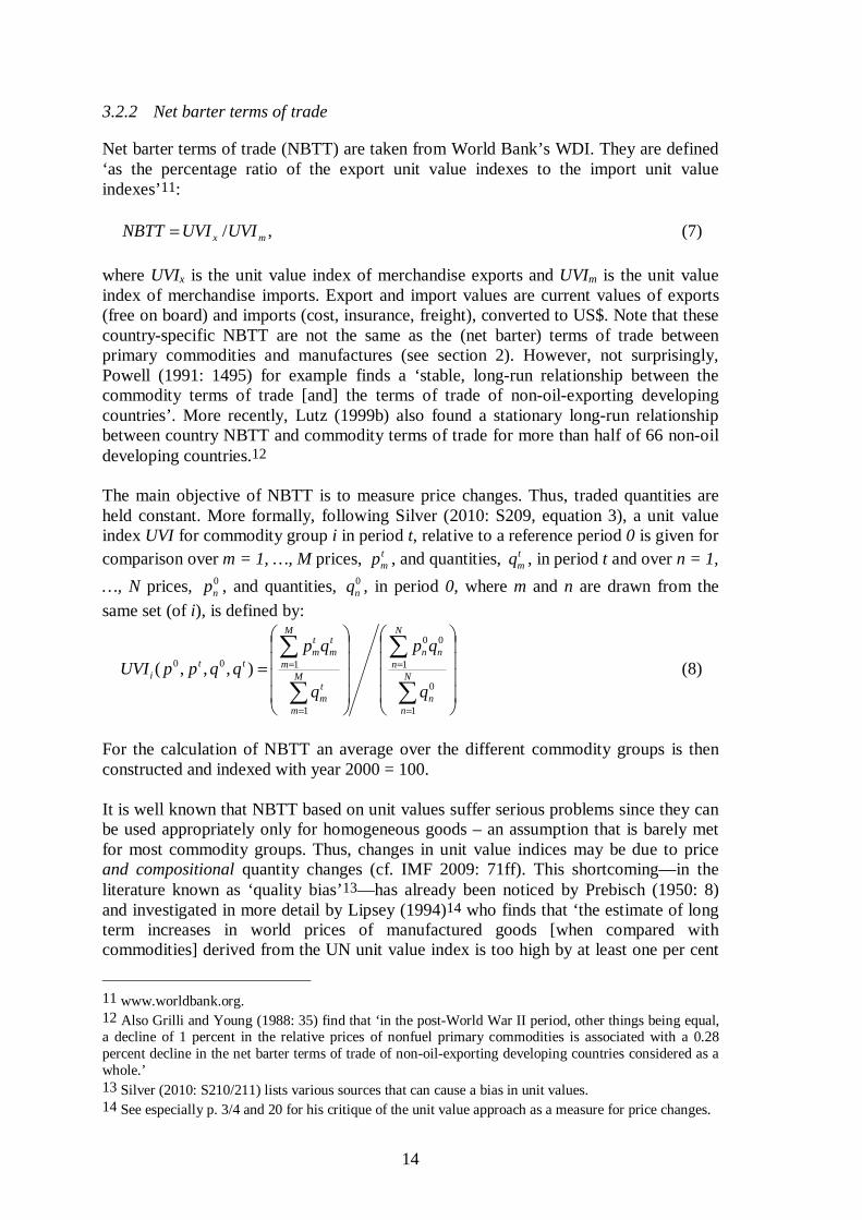
Net barter terms of trade (NBTT) are taken from World Bank’s WDI. They are defined ‘as the percentage ratio of the export unit value indexes to the import unit value indexes’11:

,/ mx UVIUVINBTT = (7) where UVIx is the unit value index of merchandise exports and UVIm is the unit value index of merchandise imports. Export and import values are current values of exports (free on board) and imports (cost, insurance, freight), converted to US$. Note that these country-specific NBTT are not the same as the (net barter) terms of trade between primary commodities and manufactures (see section 2). However, not surprisingly, Powell (1991: 1495) for example finds a ‘stable, long-run relationship between the commodity terms of trade [and] the terms of trade of non-oil-exporting developing countries’. More recently, Lutz (1999b) also found a stationary long-run relationship between country NBTT and commodity terms of trade for more than half of 66 non-oil developing countries.12 The main objective of NBTT is to measure price changes. Thus, traded quantities are held constant. More formally, following Silver (2010: S209, equation 3), a unit value index UVI for commodity group i in period t, relative to a reference period 0 is given for comparison over m = 1, …, M prices, t

mp , and quantities, tmq , in period t and over n = 1,

…, N prices, 0np , and quantities, 0

nq , in period 0, where m and n are drawn from the same set (of i), is defined by:

⎟⎟⎟⎟

⎠

⎞

⎜⎜⎜⎜

⎝

⎛

⎟⎟⎟⎟

⎠

⎞

⎜⎜⎜⎜

⎝

⎛

=∑

∑

∑

∑

=

=

=

=N

nn

N

nnn

M

m

tm

M

m

tm

tm

tti

q

qp

q

qpqqppUVI

1

0

1

00

1

100 ),,,( (8)

For the calculation of NBTT an average over the different commodity groups is then constructed and indexed with year 2000 = 100. It is well known that NBTT based on unit values suffer serious problems since they can be used appropriately only for homogeneous goods – an assumption that is barely met for most commodity groups. Thus, changes in unit value indices may be due to price and compositional quantity changes (cf. IMF 2009: 71ff). This shortcoming—in the literature known as ‘quality bias’13—has already been noticed by Prebisch (1950: 8) and investigated in more detail by Lipsey (1994)14 who finds that ‘the estimate of long term increases in world prices of manufactured goods [when compared with commodities] derived from the UN unit value index is too high by at least one per cent

11 www.worldbank.org. 12 Also Grilli and Young (1988: 35) find that ‘in the post-World War II period, other things being equal, a decline of 1 percent in the relative prices of nonfuel primary commodities is associated with a 0.28 percent decline in the net barter terms of trade of non-oil-exporting developing countries considered as a whole.’ 13 Silver (2010: S210/211) lists various sources that can cause a bias in unit values. 14 See especially p. 3/4 and 20 for his critique of the unit value approach as a measure for price changes.

15

per year’ (p. 22) mainly due to quality improvements. Grilli and Yang (1986: 33f), however, argue that previous studies of the quality bias cannot assume away the cumulative trend decline in commodity terms of trade. On the other hand, using monthly data for Germany and Japan between 1996 and 2006, Silver (2007: 14) finds that ‘month-on-month ToT indices had the wrong sign in over one-third of the month-on-month comparison’ and thus concludes that ‘the results from using UVIs to measure the terms of trade effect … were seriously misleading’ (2007: 21). Nevertheless, we do rely on UVI-based NBTT here for justified reasons besides from their ‘main advantage of … their coverage and relatively low resource cost’ (Silver 2010: S211). First, because many developing countries have considerably enlarged their manufacturing export share which weakens the point made by Lipsey (1994) in the context of commodities-manufactures trade. Second, because falling terms of trade due to quality improvements in the industrialized countries’ goods would still mean a relative impoverishment of the developing countries that could not benefit equally from world’s technical progress – a main argument of Prebisch and Singer. And third, because the economic debate on terms of trade has widely focused on UVI-based net barter terms of trade. Finally, Spraos (1983: 60, see also 58-60 for a review of the early debate on the ‘quality bias’) makes an interesting point in the debate on the ‘quality bias’ by asking how to assign the quality improvements of a manufactured article among the inputs. However, it is important to keep these limitations in mind. The aim of this paper is to give a first empirical insight into the relationship between FDI and terms of trade. Future work on the issue will have to go into more details to identify the economic channels more precisely, which also gives space to use more sophisticated terms of trade indices.

3.2.3 Other controls

The remaining control variables are listed in Table 1. Measures for world industrial production, Oilprices, and World GDP were extracted from IMF IFS. All remaining data were taken from World Bank WDI. Their interpretation should be straightforward after the discussion in section 2.2. The only variable that remains to be explained is the ‘growth deviation’ which simply is the year-by-year deviation from the average GDP per cent per annum growth trend over the whole period under consideration. This variable tries to capture cyclical influences on terms of trade.

3.2.4 Descriptive statistics

Figure 1 shows the development of net barter terms of trade (indexed here with 1980 = 100) and the FDI/GDP ratio (as explained in section 2.2.1) during the period under investigation. The data is an un-weighted average over the country groups following World Bank’s income classification. Generally, the same tendency is seen for both groups: terms of trade suffered a considerable decrease (-22 per cent for low income countries, -14 per cent for medium-low income countries) whereas the importance of FDI has increased for both types of countries (+392 per cent in low income countries, +316 per cent in medium-low income countries). Between 1989 and 1995 the main increases of FDI stocks took place in Mongolia, Cuba, Mozambique, Uganda, and Lao

16

in relative terms and in Liberia, Equatorial Guinea, Guyana, Dominica, and St. Vincent and the Grenadines in absolute terms.15

Figure 1: Development of FDI and NBTT, 1980-2008

100

120

140

160

NB

TT (i

ndex

)

1020

3040

5060

FDI s

tock

(% o

f GD

P)

1980 1990 2000 2010year

FDI mediumlow income countries FDI low income countriesNBTT mediumlow income NBTT low income

Sources: UNCTAD and World Bank (see section 3.2 of this paper). Table 1 reports the means, standard deviations and numbers of observations for all variables under consideration. This is done for all countries as well as for country groups, providing the possibility to interpret the size of estimated coefficients in chapter 4 and giving some information about the differences between different types of countries. It can be seen, for example, that developing countries, especially low-income countries, are considerably more abundant to agricultural exports. On the reverse, the importance of the industrial sector is not as important. The domestic relevance of the service sector in low-income countries is only about 2/3 of the high-income countries’ level. When looking at NBTT and the growth rate of GDP we find that volatility (i.e. the standard error) is considerably higher in low-income countries than in the rest of the data set.

15 The dramatic increase of low-income countires’ FDI ratio from the late 1980s to the mid-1990s is especially driven by Liberia, where FDI stock rose from about 200 to 2,000 per cent of GDP before it fell below 1,000 per cent again. However, also excluding such singular cases there can be no doubt that the importance of FDI has risen in low-income countries throughout the period under investigation.

17

Table 1: Descriptive Statistics

All Countries High Income Countries Medium-High Income Medium-Low Income Low income Countries

Variable Mean Std. Dev. Obs Mean Std. Dev. Obs Mean Std. Dev. Obs Mean Std. Dev. Obs Mean Std. Dev. Obs

NBTT 109.296 40.096 3,220 102.311 18.693 648 108.409 36.056 456 106.349 31.363 1,123 117.595 56.294 993

FDI (stock / GDP) 30.409 74.639 4,786 26.157 34.498 899 29.735 36.008 789 30.306 35.751 1,688 33.620 126.029 1,410

Agricultural raw materials exports

(% of merchandise exports) 6.365 11.147 4,698 3.396 5.029 1,193 3.111 5.327 923 6.118 8.702 1,604 13.463 18.551 978

Current account balance (% of GDP) -3.602 10.852 4,702 1.169 12.216 989 -2.743 9.719 832 -4.744 9.009 1,682 -6.530 11.399 1,199

Employment in agriculture

(% of total employment) 18.950 18.236 2,133 5.336 3.335 676 13.521 9.762 552 27.232 16.731 721 52.804 15.777 184

Employment in industry

(% of total employment) 25.225 7.928 2,141 27.750 5.475 677 28.826 7.643 558 22.610 7.423 722 15.278 6.305 184

GDP per capita (constant 2000 US$)’ 5,943.8 8,931.7 6,013 20,558.8 9,509.6 1,241 5,450.4 3,496.7 1,061 1,792.7 1,260.0 2,126 399.1 532.5 1,585

Industry, value added (% of GDP) 30.172 12.893 5,385 36.148 12.319 1,004 35.542 13.610 955 30.327 10.669 1,882 22.775 11.498 1,544

Inflation, GDP deflator (annual %) 46.280 521.108 6,056 7.580 19.254 1,263 42.256 202.012 1,062 73.307 627.076 2,095 44.159 687.873 1,636

Labour force, total 14,000,000 58,100,000 5,159 12,400,000 26,000,000 954 8,997,792 18,400,000 870 5,623,243 7,969,042 1,827 28,200,000 103,000,000 1,508

Labour participation rate, total

(% of total population ages 15+) 64.024 10.154 5,162 62.166 7.627 957 58.647 7.317 870 62.111 8.462 1,827 70.624 11.475 1,508

Manufactures exports

(% of merchandise exports) 38.165 30.978 4,707 54.883 32.103 1,201 41.239 31.091 926 31.517 25.556 1,605 25.594 28.084 975

Real effective exchange rate index

(2000 = 100) 2,473 100,153 2,809 101.265 18.975 865 108.365 55.940 537 7,732 180,130 868 166.131 219.129 539

Real interest rate (%) 5.931 19.345 3,909 5.369 14.555 807 5.424 15.324 661 7.051 26.165 1,380 5.218 13.389 1,061

Services, etc., value added (% of GDP) 50.819 14.037 5,388 60.129 12.313 1,008 55.698 14.896 955 52.023 11.575 1,882 40.250 10.183 1,543

Trade (% of GDP) 77.637 44.558 5,774 83.844 54.972 1,111 86.965 45.119 995 82.432 36.204 2,005 62.128 41.639 1,663

Unemployment, total

(% of total labour force) 8.928 5.915 2,182 7.018 3.881 715 10.324 5.337 521 10.299 6.909 746 7.006 6.881 200

average GDP p.c. growth rate 0.020 0.021 7,215 0.019 0.011 1,404 0.022 0.014 1,365 0.021 0.022 2,574 0.017 0.028 1,872

deviation from average GDP p.c.

growth rate 0.000 0.058 5,827 0.000 0.036 1,204 0.000 0.063 1,026 0.000 0.061 2,060 0.000 0.065 1,537

World Average Crude Oil Price 9.976 5.095 6,698

Industrial Production of Advanced

Economies 78.014 16.241 6,698

World GDP (index) 188.991 63.431 6,698

Sources: UNCTAD and World Bank (see section 3.2 of this paper).

18

3.2.5 Unit root tests

Even though it is a rather simple fact that panel data consists of a cross-section and a time series component, the problem of spurious regression (cf. Granger and Newbold 1974; Granger 1990) in the presence of a unit root is ‘usually ignored in applied economics’ (Entorf 1997: 291) in a panel context (for further details see Kao 1999). To perform the test, a Fisher test statistic proposed by Maddala and Wu (1999) is used since it is more powerful than other tests (such as an IPS test) in distinguishing the null and the alternative hypothesis (see Maddala and Wu 1999: 645) and the test needs no balanced panel, can be used for different lag lengths in the individual regressions (Maddala and Wu 1999: 636) and allows for missing observations in the series, which is an important advantage in the present investigation. The test statistic is defined as

∑=

−=N

ii

1

)log(2 ππ , (9)

where πi denote the p-value of any unit root test for cross-section/country i and π follows a 2χ distribution with 2N degrees of freedom. Contrary to (asymptotic) test statistics based on the idea of the IPS test, the Fisher test thus is an exact test based on combining the significance levels. The STATA-module written by Merryman (2004) is used to conduct the test.

Table 2: Test statistic for ln(NBTT) unit root test

no lag 1 lag 2 lags 3 lags

no trend 320.9* 435.0*** 344.4** 380.3***

with tend 354.6** 470.0*** 358.7*** 219.6 Note: ***, **, * means that one can reject the null of a unit root at the 1%, 5%, 10% level of statistical significance, respectively. Degrees of Freedom for all tests: 286. Sources: UNCTAD and World Bank (see section 3.2 of this paper). The results in Table 2 allow rejecting the null hypothesis of a unit root for the ln(NBTT) series for up to 2 lags with a time trend and general rejection without trend (although only at the 10 per cent level with no lag).

4 Results

4.1 A simple OLS model

While at first view Figure 1 may suggest FDI to be negatively related with NBTT over time, more conclusive insight is given by a simple parametric regression reported in Table 3. I start with a model that allows for different impacts of lagged FDI on ln(NBTT) for different types of countries and follow the approach of Ziesemer (2010) to also have different time trends for these types of countries. Similar to Spraos (1983: 112) this time trend could be interpreted as a ‘super-reduced form’ of a structural model. Since the NBTT index is a highly persistent series I include a lagged dependent

19

variable in specification (2). This reflects the fact that the last period’s value will potentially be a good predictor for this period. That this is indeed the case can be seen from the remarkably increased R-squared. The time trends show long-run coefficients of -0.99 per cent per annum and +0.9 per cent per annum for low-income and low-medium income countries respectively.16 This is fairly different from the respective values of -0.42 per cent and -0.02 per cent observed by Ziesemer (2010: table 1) in a pure time-series AR(2) specification. The impact of lagged FDI on ln(NBTT) is estimated to be positive and statistically (at least weakly) significant for developing countries. Including time dummies (specification (3)), this effect does not change considerably but standard errors are now somewhat higher for low-medium-income countries so that weak statistical significance is not assured anymore.

Table 3: FE Regression, dependent variable: ln(NBTT)

(1) (2) (3)

Lagged Dependent Variable -

0.8890***

(0.0153)

0.8859***

(0.0152)

Trend

high income 0.0044***

(0.0009)

0.0003

(0.0004)

0.0020***

(0.0007)

med-high income 0.0035

(0.0023)

0.0038***

(0.0010)

0.0057***

(0.0012)

low-med income -0.0020**

(0.0010)

0.0010**

(0.0005)

0.0027***

(0.0007)

low income -0.0137***

(0.0015)

-0.0011

(0.0008)

0.0005

(0.0010)

FDI(-1)

high income -0.0008**

(0.0004)

0.0001

(0.0001)

-0.0000

(0.0001)

med-high income -0.0014*

(0.0008)

-0.0006

(0.0004)

-0.0007

(0.0005)

low-med income -0.0009*

(0.0005)

0.0005*

(0.0003)

0.0004

(0.0003)

low income 0.0017

(0.0011)

0.0014**

(0.0006)

0.0014**

(0.0006)

Time Dummies No No Yes

F-stat (prob) 0.0000 0.0000 0.0000

R within 0.0658 0.7564 0.7662

No. of Obs. 3,032 2,977 2,977

Sources: UNCTAD and World Bank (see section 3.2 of this paper).

16 Long-run coefficients are calculated by dividing the coefficient for the time trend by (1 – coefficient of the lagged dependent variable).

20

4.2 The full LSDV model and sub-models

For the next step, I include all variables relevant for the world market approach (cf. subsection 3.1.3) in the model (4) in Table 4. Lagged FDI stock still has a positive and statistically significant impact on ln(NBTT) for low-income countries, although the sample size drastically decreased when compared to the specifications reported in Table 3. The size of the parameter estimate is now almost fivefold the size it was before. For medium-low income countries, the estimate is positive and weakly significant, being about double the size of specification (2).

Table 4: FE regression, dependent variable: ln(NBTT)

(4) (5) (6) (7)

Lagged Dependent Variable

0.7520*** (0.0401)

0.7656*** (0.0380)

0.8180*** (0.0346)

0.7714*** (0.0553)

Trend

high-income 0.0092*** (0.0021)

0.0091*** (0.0020)

0.0055*** (0.0017)

-

med-high income

0.0044* (0.0026)

0.0060*** (0.0022)

0.0036* (0.0018)

-

low-med income

0.0080*** (0.0022)

0.0072*** (0.0020)

0.0061*** (0.0017)

-0.1104** (0.0538)

low-income -0.0020 (0.0045)

-0.0017 (0.0026)

-0.0020 (0.0021)

-0.1169** (0.0542)

FDI(-1)

high-income 0.0001 (0.0002)

0.0002 (0.0002)

0.0002 (0.0001)

-

med-high income

0.0001 (0.0007)

0.0002 (0.0007)

0.0005 (0.0006)

-

low-med income

0.0012* (0.0007)

0.0017*** (0.0006)

0.0012** (0.0006)

0.0017* (0.0010)

low-income 0.0068*** (0.0012)

0.0098*** (0.0017)

0.0094*** (0.0016)

0.0067*** (0.0020)

Agricultural Raw Material Exports (% of GDP)

0.0024* (0.0013)

0.0012 (0.0011)

- 0.0011 (0.0018)

Current Account Balance (% of GDP)

0.0083*** (0.0016)

0.0066*** (0.0014)

0.0071*** (0.0015)

0.0060* (0.0031)

Current Account Balance (% of GDP) (-1)

-0.0075*** (0.0016)

-0.0063*** (0.0014)

-0.0058*** (0.0014)

-0.0035 (0.0025)

Employment in Agriculture (% of total employment)

-0.0002 (0.0008)

- - 0.0014 (0.0013)

Employment in Industry (% of total employment)

-0.0007 (0.0022)

- - 0.0028 (0.0043)

GDP p.c. (constant 2000 US$)

-0.0000** (0.0000)

-0.0000** (0.0000)

-0.0000 (0.0000)

-0.0000 (0.0000)

Industry Value Added (% of GDP)

0.0072*** (0.0028)

0.0066*** (0.0017)

0.0036** (0.0016)

0.0045 (0.0043)

Inflation (GDP deflator, annual %)

-0.0001*** (0.0000)

-0.0000*** (0.0000)

-0.0000*** (0.0000)

-0.0001*** (0.0000) table continues…

21

ln(Labourforce) 0.0243*** (0.0053)

0.0246*** (0.0051)

0.0217*** (0.0050)

-0.0001*** (0.0000)

Labour participation rate (% of total population)

0.0001 (0.0021)

- - -0.0006 (0.0059)

Manufactures Export (% of merchandise exports)

-0.0001 (0.0006)

0.0002 (0.0005)

-0.0003 (0.0005)

-0.0003 (0.0007)

Real Effective Exchange Rate

0.0019*** (0.0003)

0.0015*** (0.0003)

0.0012*** (0.0002)

0.0025*** (0.0006)

Real Interest Rate (%) -0.0001 (0.0005)

-0.0000 (0.0005)

- 0.0022** (0.0010)

Services etc. Value Added (% of GDP)

0.0003 (0.0024)

- - -0.0003 (0.0033)

Trade (% of GDP) -0.0008** (0.0003)

-0.0007* (0.0004)

-0.0005 (0.0004)

-0.0009 (0.0006)

Unemployment (% of total labour force)

0.0014 (0.0014)

0.0013 (0.0011)

0.0004 (0.0010)

0.0034 (0.0023)

Growth Deviation 0.4551*** (0.1361)

0.3700*** (0.1267)

0.3349*** (0.1236)

0.6278*** (0.2398)

Growth Deviation (-1) -0.2536** (0.1116)

-0.3430*** (0.1049)

-0.3345*** (0.1023)

-0.4367** (0.1950)

Oilprice - - -

-0.0450** (0.0173)

Industrial Production - - -

-0.0015 (0.0045)

World GDP - - -

0.0175** (0.0073)

Time Dummies yes yes yes yes F-statistic (prob) 0.0000 0.0000 0.0000 0.0000 R squared within 0.8073 0.7928 0.7865 0.8547 No. of Obs. 713 773 876 225 Sample whole sample whole sample whole sample developing

countries Estimation method FE robust FE robust FE robust FE robust

Sources: UNCTAD and World Bank (see section 3.2 of this paper). T-tests for joint significance of the time dummies in model (4) do not allow to reject the null hypothesis that the time dummies are not jointly significant, however, results concerning FDI for developing countries remain about the same size and are statistically significant at the same levels if time dummies are removed. A Hausman test clearly allows rejection of the null hypothesis that the difference between a fixed effect and a random effect model is not systematic, at the 5 per cent (and also the 1 per cent) level of significance. This implies that the fixed effect specification is the correct one here because a random effects model would be inconsistent. Finally, I use a likelihood-ratio test to investigate whether a model with only one parameter for the influence of FDI, i.e. not regarding different effects of FDI on NBTT between country types, provides the same fit as the full model in specification (4). The test statistic allows rejecting the null hypothesis that the reduced model provides the

22

same fit at the critical 5 per cent value. The same procedure allows rejection that time trends do not vary between countries (rejection is possible even at the 1 per cent level). It should be noted, though, that all specifications here produce a distribution of residuals that differs from a normal distribution. Hence, conventional inference, especially the t-statistic, may be misleading. In the next step, some intuitive model selection was carried out. Note that any kind of model selection will result in underestimation of standard errors and therefore biased inference (cf. Pötscher 1991), although compared to many other empirical studies the problem of incorrect inference is less severe because the data has not been used in a comparable model before.This process will also indicate how robust the estimates from model (4) are. In a first step, the employment shares of agriculture and industry, the labour participation rate and the share of services in total value added were excluded, leading to model (5). The positive impact of FDI on NBTT is then stronger in size (by almost 50 per cent) for developing countries and increased also in significance; it is now statistically significant also for medium-low-income countries and highly significant for low-income countries. When also excluding the share of agricultural raw material exports and the real interest rate, estimates are still significant and within the range spanned by the estimates before (see model (6)). It is worth mentioning that in further selection procedures, elimination of manufacturing exports, real effective exchange rate17 and unemployment rate led to insignificant results for the impact of lagged FDI on ln(NBTT) for developing countries.18 Also note that the coefficient of the lagged dependent variable is significantly smaller than 1, which further supports the findings of section 3.2.5 that there is no unit root in the series.

4.2.1 The Model for Developing Countries

In the next step I apply model (6) exclusively to developing countries in the sample. Since Oilprice, World GDP and World Industrial Production are expected to be important for terms of trade of these countries they enter the model as explanatory variables. The first two of them turn out to be statistically significant (see model (7) in Table 4). For the impact of lagged FDI on ln(NBTT), parameter estimates are comparable to the results obtained before. However, an important observation is that the residuals from the developing country subsample seem to come closer to a normal distribution than the residuals from the industrialized country subsample. It thus seems that the model, which mainly focuses on market forces, describes terms of trade for developing countries more appropriate than for industrialized countries. This finding is also fostered by the fact that the coefficient of determination, R-squared, is higher for the developing country subsample than for industrialized countries.

17 The real effective exchange is negatively correlated with FDI, thus not controlling for it leads to an ambiguous effect of FDI on NBTT: On the one hand a negative effect via the exchange rate and a positive direct effect on the other hand leading to an overall effect that is not significantly different from 0. 18 Parameter estimates for the impact of FDI on NBTT reported in Table 5 are also statistically significant when manufacturing exports are excluded.

23

Table 5: FE regression, dependent variable: ln(NBTT)

(8) (9) (10) (11) Lagged Dependent Variable

0.7601*** (0.0549)

0.7492*** (0.0554)

0.8016*** (0.0389)

0.8016*** (0.0389)

FDI(-1) 0.0019** (0.0009)

0.0019** (0.0009)

0.0011*** (0.0003)

0.0011*** (0.0003)

Agricultural Raw Material Exports (% of GDP)

0.0010 (0.0019) - - -

Current Account Balance (% of GDP)

0.0065** (0.0029)

0.0065** (0.0028)

0.0077*** (0.0024)

0.0077*** (0.0024)

Current Account Balance (% of GDP) (-1)

-0.0040* (0.0024)

-0.0040* (0.0024)

-0.0037* (0.0020)

-0.0037* (0.0020)

Employment in Agriculture (% of total employment)

0.0016 (0.0013)

0.0008 (0.0006)

0.0008 (0.0005)

0.0008 (0.0005)

Employment in Industry (% of total employment)

0.0034 (0.0043) - - -

GDP p.c. (constant 2000 US$)

-0.0000 (0.0000)

-0.0000 (0.0000)

0.0000** (0.0000)

0.0000** (0.0000)

Industry Value Added (% of GDP)

0.0038 (0.0036)

0.0042 (0.0032)

0.0016 (0.0011)

0.0016 (0.0011)

Inflation (GDP deflator, annual %)

-0.0001*** (0.0000)

-0.0001*** (0.0000)

-0.0000*** (0.0000)

-0.0000*** (0.0000)

ln(Labourforce) 0.0380*** (0.0106)

0.0377*** (0.0099)

0.0148* (0.0078)

0.0148* (0.0078)

Labour participation rate (% of total population)

-0.0004 (0.0054) - - -

Manufactures Export (% of merchandise exports)

-0.0003 (0.0007)

-0.0003 (0.0007)

0.0000 (0.0003)

0.0000 (0.0003)

Real Effective Exchange Rate

0.0025*** (0.0006)

0.0026*** (0.0006)

0.0013*** (0.0004)

0.0013*** (0.0004)

Real Interest Rate (%) 0.0024** (0.0009)

0.0023** (0.0009)

0.0009 (0.0007)

0.0009 (0.0007)

Services etc. Value Added (% of GDP)

-0.0006 (0.0032) - - -

Trade (% of GDP) -0.0009 (0.0006)

-0.0008 (0.0006)

-0.0004*** (0.0002)

-0.0004*** (0.0002)

Unemployment (% of total labour force)

0.0039* (0.0023)

0.0026 (0.0019)

0.0028*** (0.0010)

0.0028*** (0.0010)

Growth Deviation 0.6787*** (0.2273)

0.6700*** (0.2217)

0.6410*** (0.2438)

0.6410*** (0.2438)

Growth Deviation (-1) -0.4228** (0.1972)

-0.4189** (0.1871)

-0.2820 (0.1999)

-0.2820 (0.1999)

Oilprice -0.0452** (0.0056)

-0.081** (0.0041)

-0.0049 (0.0090)

-0.0062 (0.0041)

Industrial Production -0.0041 (0.0041) - - -

World GDP 0.0029** (0.0013)

0.0018*** (0.0006)

0.0027*** (0.0007)

0.0010* (0.0005)

Time Dummies yes yes yes yes F- /Chi²-statistic (prob) 0.0000 0.0000 0.0000 0.0000 R squared within 0.8528 0.8521 0.8350 0.8964 No. of Obs. 225 225 225 225 Sample developing

countries developing countries

developing countries

developing countries

Estimation method FE robust FE robust RE robust POLS robust Sources: UNCTAD and World Bank (see section 3.2 of this paper).

24

Applying a likelihood ratio test does not allow rejecting the null hypothesis that a reduced model with a common time trend and a common parameter for the impact of lagged FDI on ln(NBTT) provides the same fit as the model in specification (7). Accordingly, model (7) is re-estimate with a common parameter for FDI without time trend since a common linear time trend for all subgroups can also be represented through time dummies included in the model. The results are presented in specification (8) in Table 5. Time dummies of the model are jointly statistically significant at the 5 per cent level. In specification (9) I use the model (6) that has been derived in the full sample, now applied only to developing countries and also include World GDP and Oilprice. This is the preferred specification of this investigation and again time dummies are jointly statistically significant at the critical 5 per cent level. Note, that standard errors are more appropriate here than in the models of Table 4 because the dataset used in model (9) somewhat differs from the full sample where model selection has been carried out. Since a Hausman test does not allow rejecting the null hypothesis that the difference between fixed effect and random effect estimation is not systematic, Table 5 also reports the results of random effect estimation in specification (10).19 While the sign of the coefficients and their statistical significance generally stays unaffected (only the impact of GDP p.c. turns to positive and significant, significance of some other parameters changes), the size of the parameter estimates may differ. The impact of lagged FDI on ln(NBTT), for example, considerably decreases from 0.19 per cent to 0.11 per cent. For comparison, the results of pooled OLS are also reported in specification (11) which essentially provides the same estimates as random effects. This also allows comparison of the fixed effects estimator for the lagged dependent variable in (9) with the estimation using pooled OLS in (11). As we might expect from standard results for omitted variables bias in finite samples, the coefficient of the generally downward biased fixed effects estimator is smaller than the generally upward biased pooled OLS levels estimator (cf. Bond 2002: 4-5).

4.2.2 Some tests

So far, the empirical results show that lagged FDI stock has a positive and statistically significant impact on ln(NBTT). Although OLS results in a setting with a lagged dependent variable will be biased (see section 4.3 below), I provide some tests to support the statistical significance of the results and to investigate possible economic channels of the relationship.20 For the previous models a Huber (1967)-White (1980) sandwich estimator was used to estimate the variance of the estimators and provide corresponding inference (such as t-statistics). A Wooldridge (2002; Drukker 2003) test for serial correlation rejects the null hypothesis of no autocorrelation in the residuals for the preferred model (9). Two

19 Note, that a Hausman test for the same model but applied to high and medium-high income countries would clearly allow rejection of the null hypothesis (χ2 statistic of 248.72 with 42 degrees of freedom). 20 I apply the tests within the OLS framework because splitting the (already small) sample would impose serious restrictions to the moment conditions when applying GMM and supposably increase standard errors which would decrease the power of the tests. Since we can expect the bias of the OLS estimator to be the same for both sub-samples tested against each other, the OLS model provides a reasonable testing framework.

25

approaches may address the issue. Using a ‘Newey-West procedure’ produces a standard error of 0.000939 that means the estimate for the impact of lagged FDI stock is statistically significant. If we allow for more than one lag of autocorrelation, the estimate is no more significant on the 5 per cent level but clearly on the 10 per cent level (for example, t-statistic of 1.92 for 5 lags). The other option is to cluster observations on the country level (cf. Froot 1989; Rogers 1993; Wooldridge 2002: sec. 13.8.2) which does not assume them to be independent within each cross-section. Using robust clustered standard errors provides a t-statistic of 1.88 (standard error 0.0009888), i.e. again the impact of lagged FDI stock on ln(NBTT) is significant on the 10 per cent but not on the 5 per cent level. Another potential shortcoming might arise if the nature of FDI changed throughout the time period investigated. For example, FDI to developing countries might have become more concentrated in the service sector or the growing importance of South-South FDI might have different impacts on ln(NBTT). If this is the case, the relationship between lagged FDI stock and ln(NBTT) would have changed over time. To investigate this issue I estimate an equation of the form:

εθββα rr+Ψ+++=

∧

−≥

∧

−<

∧∧

it1,)(21,)(1 )(1)(1)ln( titttittiit FDItFDItNBTTjj

, (10) where 1 is the indicator function and tj is a certain breakpoint in time. The test hypothesis of interest is then H0: β1 – β2 = 0, which means that β1 = β2, i.e. they are not significantly different from each other. The according test statistic will then follow a t-distribution and does neither allow rejecting the null hypothesis for tj = 1990 nor for tj = 1997, no matter whether equation (10) is estimated with or without time dummies. To investigate possible economic channels of the FDI-NBTT relationship I use a test statistic similar to the one derived from equation (10). Therefore, I split the developing countries under investigation into two groups. Group A lies above the median of a certain measure and group B lies below. I then estimate the equation

εθββα rr+Ψ+++=

∧

−∉

∧

−∈

∧∧

it1,)(21,)(1 )(1)(1)ln( tiAitiAiiit FDIiFDIiNBTT (11)

and again test whether H0: β1 – β2 = 0 for criteria such as 1985 GDP percentage, ratio of agricultural exports to GDP in 1980, average GDP percentage growth rate, trade/GDP rate in 1985 and 2000. For neither measure it is possible to reject the null hypothesis on the 5 per cent level but we can reject H0 at the 10 per cent level of statistical significance for the trade/GDP ratio, i.e. the positive relationship between FDI and NBTT is stronger in countries that have a higher trade/GDP ratio. This, however, does not necessarily mean that more open economies experience a stronger FDI-NBTT relationship. Taking the Sachs-Warner (1995) openness measure as a criterion to separate group A from B does not allow rejecting the null hypothesis of equal parameters for both groups. This issue will be discussed in more detail in section 5.2. Finally, I apply a robustness check using a newly constructed FDI stock series based on the perpetual inventory method. The reason therefore is that FDI stock values might suffer from problematic asset valuation: While the IMF (1993: §376) suggests using market values for FDI, it also recognizes (§377) that ‘in practice, book values from the balance sheets of direct investment enterprises (or investors) often are used to determine the value of the stock of direct investment’ since enterprise balance sheet values are a source readily available in most countries. However, book values might not be a good

26

measure for the economic implication of an asset in a host economy, especially if the original investment dates back many years and balance sheets are based on historical cost basis, since depreciation rates are subject to a multinational’s global profit maximization and not to an economically adequate measurement of assets’ performance. For example, a high-tech machine of a world-leading multinational might still be relatively state-of-the-art and in full operation, even though being fully depreciated, while another firm’s equipment, highly outdated, might have some book value even after 9 years. To overcome this potential problem I use the fact that FDI stock consists of past FDI flows and construct a different series for FDI stocks using the perpetual inventory method. This is legitimate because neglecting asset price changes and exchange rate movements as well as other small adjustments, the difference between the FDI stock at the beginning of the year and its value at year-end must be equal to the net flow recorded in the Balance of Payments and also provided by UNCTAD FDIstats. The method is described in more detail in appendix A3 but generally estimates the FDI stock St in year t as:

,)1( 11 −− +−= ttt FSS δ (12)

where δ is the depreciation rate and Ft is the FDI flow in year t. Note that this is simply a geometric depreciation of the past stock, adding the new flow. I use the method of Hall and Jones (1999: 89) to estimate initial values S0 of FDI stock and assume a depreciation rate of δ = 0.1. While this seems rather high at a first view, it is discussed in the appendix why it is the most appropriate one. Specification (7) shows a statistically significant impact of lagged FDI on NBTT for

medium-low-income countries ( 00127.0*,*00287.0 ==∧

SEβ ), but no significant

impact for low-income countries ( 00723.0,00674.0 ==∧

SEβ ). The findings for the other specifications are reported in Table 6.

Table 6: Robustness Check, parameter estimate for FDI(-1)

Specification same as (8) same as (9) same as (10) same as (11) ∧β (and robust SE) for FDI(-1)

0.002472* (0.0012728)

0.0023184** (0.0011558)

0.0006718 (0.0004774)

0.0006718 (0.0004774)

with δ = 0.01 0.0021527** (0.0010843)

0.0019715* (0.0010247)

-2.68e-06 (0.0000249)

-2.68e-06 (0.0000249)

with δ = 0.05 0.0024612** (0.0012072)

0.0023174** (0.0011094)

0.0004114 (0.0003865)

0.0004114 (0.0003865)

with δ = 0.15 0.0025184* (0.0014143)

0.0023432* (0.0012577)

0.0010521* (0.000614)

0.0010521* (0.000614)

with δ = 0.2 0.0025883 (0.001574)

0.0023928** (0.0013741)

0.0013056* (0.000728)

0.0013056* (0.000728)

with δ = 0.25 0.0026482 (0.001748)

0.0024406 (0.0015016)

0.0014742* (0.0008293)

0.0014742* (0.0008293)

with δ = 0.5 0.0026587 (0.0026331)

0.0025119 (0.0021715)

0.0018283 (0.0012583)

0.0018283 (0.0012583)

Sources: UNCTAD and World Bank (see section 3.2 of this paper).

27

As it turns out, the estimates for the influence of lagged FDI stock on ln(NBTT) are still significant (for specification (9), weakly significant in specification (8)) and positive. The estimates are somewhat higher using the newly constructed FDI stock, but note that the difference is not significant as the standard errors of the estimators overlap. Another interesting finding of the robustness check is that also depreciation rates of δ = 0.05 and δ = 0.15 provide (at least weakly) significant and positive results (for specifications (8) and (9) at least). For depreciation rates of δ = 0.2 and above significance generally drops. Note that for δ → 1, St → Ft, meaning that with increasing depreciation rate, stocks will converge against the value of flows. This finding is interesting from an economic perspective because it tells us, that the positive impact of FDI on net barter terms of trade is not a short one that comes from influences on the balance of payments etc but rather has a long-lasting impact. The issue will be discussed further in section 5.2.

4.3 Parameter identification: A GMM approach

So far, different OLS techniques were used to estimate the parameters of interest. However, there are two major shortcomings of using OLS. Firstly, in the presence of lagged dependent variables the OLS estimate will be biased (see Appendix A4). Furthermore, there might be a problem of simultaneity because in economics an investment simply captures future profits. As we know from the multinationals literature, improvements in factors such as education, custom clearance efficiency, infrastructure, and logistics will improve the future market potential and thereby attract FDI. However, it is also likely that these factors may increase export performance and thus terms of trade. Note that from the policy perspective this simultaneity is not a problem: As FDI is positive (or not significantly) related to terms of trade, government investments in education, for example, may improve product quality and thus terms of trade and by simultaneously attracting FDI, terms of trade may be improved further on. Thus, FDI does not only influence terms of trade but FDI itself will be influenced by factors determining terms of trade which leads to a biased parameter estimate. This bias is of order T-1 in panels with weak dependence21 and thus may be small (cf. Wooldridge 2002: 302); however, I use General Methods of Moment (GMM) as an alternative estimation strategy. This does not only overcome the bias from the lagged dependent variable but also provides a framework for instrumenting an explanatory variable x that is potentially simultaneous if there are no good instruments z, such that Cov(z,ε)=0 and Cov(z,x) ≠ 0, waiting in the wings. The general idea of GMM is to force r ≥ k exogenous instruments in the T x r matrix Zi to satisfy the r moment conditions E(Zi‘ εi) = 0. This leads to an estimator

YZWZXXZWZXGMM '')''( 1−∧

=β , (13)

where W is a symmetric and idempotent r x r weighting matrix. Note, that for E(Xi‘ εi) = 0 equation (13) would simplify to OLS estimation. The estimator in (13) is consistent under the assumption E(Zi‘ εi) = 0 though not generally unbiased in finite samples. It is not efficient but can be made efficient in a two-step estimation technique.

21 A series is said to be weakly dependent if Cor(yt, yt+h) → 0 as h →∞.

28

For this investigation I use the System GMM estimator proposed by Blundell and Bond (1998). The main idea is that suitably lagged first differences of a series x, ∆xi,t-s, may be uncorrelated with αi. For example, ∆xi,t-1 = xi,t-1 - xi,t-2 is mathematically related to xi,t-1 and hence the lagged dependent variable but not to εit and is thus available as an instrument. I decided to instrument the lagged FDI stock with 4 to 6 lags22 whereas the lagged dependent variable and the lagged Oilprice are instrumented with one up to 6 lags. Lagged World GDP and lagged logarithm of the labourforce as well as time dummies are used as supplementary instruments. A one-step GMM estimation with small sample correction and a Huber (1967) –White (1980) - sandwich variance estimator was used. The results for the parameter estimate of the lagged dependent variable and lagged FDI stock using the same specification as in model (9) are presented in Table 7 together with a replication of models (9) and (11) to ease comparison.

Table 7: GMM results compared to OLS, dependent variable: ln(NBTT)

Model (9) (11) (12)

System GMM

(13)

Difference GMM

LDV 0.7492***

(0.0554)

0.8016***

(0.0389)

0.8051***

(0.0437)

0.7760***

(0.0834)

FDI(-1) 0.0019**

(0.0009)

0.0011***

(0.0003)

0.0010**

(0.0004)

0.0018

(0.0013)

Other controls yes yes yes yes

Time Dummies yes yes yes yes

No. of obs / instruments 217/217 181/180

AB test for AR(1) in FD:

z-stat (pval)

-2.48

(0.013)

-2.48

(0.013)

AB test for AR(2) in FD:

z-stat (pval)

0.62

(0.534)

0.39

(0.694)

Hansen test: Chi2-stat

(pval)

165.31

(0.669)

0.0

(1.0) Sources: UNCTAD and World Bank (see section 3.2 of this paper). Comparing the results of the System GMM specification (12) with those of the fixed effect and other regressions shows that the estimated coefficient of the lagged dependent variable is larger than the generally downward biased one of the FE regression. However, contrary to standard results it also slightly surpasses the OLS estimator. But since the difference is not significant (each estimate lies clearly within the standard error of the other one) the concern for inconsistency or severe finite sample bias is not too substantial (cf. Bond 2002: 5f).23 More interesting for the purpose of this study is

22 Using lower lags does not change the estimated coefficients remarkably but produces a telltale Hansen test statistic (in all cases the p-value of the statistic is 1.000, Roodman 2006: 43). 23 For an AR(2)-specification, estimated coefficients are 0.791014 and -0.0020477 for the first and second lagged dependent variable, respectively. Thus, their sum would lie within the interval between FE and POLS estimates, just as expected. However, the second lag (standard error 0.1001979) is far from

29

the fact that the estimator for the influence of lagged FDI stock has come down to 0.00097 but is still statistically significant. Note also that estimated standard errors are rather conservative because only an inefficient one-step estimation procedure has been used.24 The System GMM estimate is statistically different from the FE estimate, i.e. the latter is not contained in the interval of one standard error around the former. The conventional test statistics support the specification of the model. The Arellano-Bond statistic rejects the null hypothesis of no first-order serial correlation just as expected, but not for second-order serial correlation. The Hansen test for overidentifying restrictions clearly does not allow rejection of the null hypothesis of joint validity of the set of instruments. Note, however, that the fact that N = 22 is somewhat worrisome (Roodman 2006: 36). Table 7 also reports the results for difference GMM (cf. Holtz-Eakin et al 1988; Arellano and Bond 1991) in model (13) which follows a similar rationale as System GMM but the estimated equation is described in first differences and potentially endogenous differences are instrumented with lagged levels. Note that there is a constant in the first-difference model since a time trend in levels will become a constant in first differences whereas a constant in the former simply cancels out. The specification yields an estimate of 0.776 for the lagged dependent variable, just between FE and POLS, as we would expect, further supporting the overall model specification. The Arellano-Bond tests show the same result as in the System GMM specification but the Hansen statistic is worrisome. The impact of lagged FDI stock is more relevant in this specification when compared with system GMM and about the same size as with FE estimation but it is no longer statistically significant. This, however, should not be overrated because standard errors are again very conservative and still relatively low (close to the 10 per cent level). Furthermore it is well-known that lagged differences are a weak instrument for a series such as FDI stock that may be close to a unit-root process, yielding to high standard errors (Bond 2002: 3).

5 Discussion and conclusion

This investigation has shown that some economic arguments in favor of the Prebisch-Singer hypothesis implicitly relied on the role of multinational corporations, attributing a negative terms of trade effect to MNCs. Using FDI/GDP ratios as a measure for the importance of MNCs in various developing countries over the general time-span 1980-2008 it has been shown that there is no empirical reason to justify this argument. Rather, the investigation has shown that there is a statistically significant and robust positive effect of lagged levels of FDI stock on the (logarithm of) developing countries’ net barter terms of trade. Since statistical significance should not be confused with economic relevance it is important to address the question: How important is FDI for the developing countries’ NBTT? What else has an impact on them?

being significant. The corresponding estimate for the impact of FDI(-1) would be .0008839 with a standard error of 0.000405 and thus being statistically significant. 24 Since the number of instruments is large compared to the number of observations, an efficient two-step procedure will not lead to meaningful results.

30

5.1 Factors determining terms of trade and their economic relevance

In specifications (8) to (13), the estimated coefficient for the impact of lagged FDI stock on ln(NBTT) ranges from 0.0010 to 0.0019. This might seem negligible in terms of economic relevance on a first view. More precisely it would mean that a 1 percentage point increase in the FDI/GDP ratio would cause a 0.10 to 0.19 per cent increase in NBTT in the short run and a 0.51 to 0.79 per cent increase in NBTT in the long run.25 Assuming a negative long-run trend of NBTT for these countries of -0.42 per cent per annum as estimated (and reported to be in the range of other studies) by Ziesemer (2010: 7) for low-income countries,26 a short-run coefficient of 0.1 per cent, as estimated in model (12) would mean that an increase in the FDI/GDP ratio by 0.0042/0.00097 = 4.34 percentage points per annum could, ceterus paribus, counter the structural deterioration in developing countries’ NBTT. But how realistic is such an increase? In 1980, the (unweighted) average FDI stock in developing countries amounted to 16.1 per cent of GDP (with a standard deviation of 28.6 per cent of GDP; 90 observations). In 2008, this figure has risen to 46.2 per cent (with a standard deviation of 59.8 per cent; 114 observations), corresponding to an increase of 3.84 per cent p.a. or (46.2 - 16.1)/28 = 1.07 percentage points p.a., on average. This means that the tendency of falling net barter terms of trade in developing countries was countered by the inflows of FDI by almost one fourth, which clearly is a considerable size. Another way to look at this result is to compare the actual change in FDI stocks relative to GDP (46.2 - 16.1, multiplied with the estimated parameter of 0.1 = 3.01) to the changes in ln(NBTT) which have fallen from 4.83 (standard deviation of 0.48; 60 observations) to 4.67 (standard deviation of 0.35; 87 observations), which equals

%3.2155.1

01.3 −=−

, (14)

meaning that the increase of FDI has countered the NBTT decrease in developing countries by more than one fifth in the short run.27 Another approach is to use the estimated coefficients to predict the 2008 net barter terms of trade using the actual 2008 FDI(-1) level and compare it to a prediction where the FDI(-1) level is kept constant at its 1980 value. Unfortunately the sample does not allow predictions for 2008 but only for 2007 and here only for eight countries. Their (unweighted average) NBTT were 107.25 in 1980 and the prediction for 2007 is 102.34. Assuming that FDI remained at its 1980 level provides a prediction of 100.72. Thus, if FDI had not changed since then, NBTT had fallen by 33.1 per cent more than they actually did.28

25 0.0010/(1-0.8051)=0.0051; 0.0019/(1-0.7601)=0.0079. 26 When simply regressing log(NBTT) on time in our sample using fixed effects, we observe a coefficient of -0.62 per cent (-0.56 per cent when including year dummies to account for shocks). Estimates are highly significant, even after correcting standard errors for autocorrelation using a Newey-West procedure, significant at the 5 per cent level when clustering standard errors at country level. 27 If we use the long-run coefficient of 0.51 per cent instead, this figure increases to more than 87 per cent. 28 The eight countries in the sample are Chile, Colombia, Costa Rica, Malaysia, Pakistan, Philippines, Paraguay, South Africa. The estimate of 33.1 per cent has to be treated with care. First of all, the estimator for the influence of FDI on NBTT has a standard error. Furthermore the prediction is volatile

31

Either way, the conclusion is pretty clear: foreign direct investment is a non-negligible factor positively influencing NBTT of developing countries. Policy makers or researchers either concerned about the long-run trend of developing countries’ terms of trade to deteriorate or about terms of trade volatility in developing countries should thus consider the impact of FDI and MNCs. However, the model used to estimate this impact also reveals other factors that may be relevant in this context. The negative impact of inflation and the positive impact of the real effective exchange rate are straightforward and well-known. More interesting are the findings concerning trade (as percentage of GDP), the current account balance (also percentage of GDP), the labour force and deviations from the long-run growth path. The impact of trade (relative to GDP) on ln(NBTT) is negative in all specifications for developing countries, though only statistically (highly) significant in specifications (10)–(12). Also note that the present investigation does not account for simultaneity. For example, falling NBTT could lead to an increase of the trade/GDP ratio in order to compensate for price-induced income losses. On the other hand, if future research reveals that an increase in the trade intensity really causes a deterioration of NBTT this casts serious doubts on conventional economic wisdom and derived policy practices (cf. also Lutz and Singer 1994).29 The statistically significant impact of the current account balance is interesting because of the adverse signs among lags and the economically relevant size of the parameter estimate.30 This distributed lag specification was initially chosen because Santos-Paulino (2010: 864) finds a ‘J-curve response’ caused by a shock in terms of trade onto the current account balance. Since the intention of this study—as well as the method and data used—clearly differs from the one by Santos-Paulino (2010), no comparisons can be made. The results nevertheless highlight the potential for further research on the dynamic relationship between terms of trade and the current account balance. Another interesting finding concerns the impact of labour market changes on terms of trade. Especially Prebisch and Lewis have seen the excess-supply of labour in developing countries as a factor negatively influencing terms of trade. Accordingly, an increase in the labour force should not increase terms of trade. Also in a neoclassical model of trade, growth in the abundant factor (labour for developing countries) might worsen terms of trade (Grilli and Yang 1988: 29). Thus, the positive (and economically

with respect to the year and the corresponding volatility of FDI flows as well as with respect to the countries included in the sample. To see this, consider the prediction for the year 2006. Here, there are nine countries in the sample, Nicarauga replacing The Philippines and Ecuador entering supplementary. The estimated difference in NBTT reduces from 33.1 per cent to 9.3 per cent. For 2001, we have 13 countries in the sample: Bolivia, Chile, China, Cameroon, Colombia, Costa Rica, Dominican Republic, Cambodia, Morocco, Nicaragua, Philippines, Paraguay, and South Africa. The estimated difference is now 7.5 per cent. Thus, 33.1 per cent is probably a high figure. On the other hand, the System GMM estimator was used here, which provides a rather conservative estimate. In any case, even a figure around 7.5 per cent should not be neglected. 29 The effect might be small in terms of economic relevance though. Using the same approach as in equation (14) reveals that the actual increase in trade/GDP accounted for ‘only’ 4.4 per cent of the developing countries terms-of-trade deterioration. 30 The negative impact of the first lag is not significant in the System GMM specification (t-statistic -1.32).

32

relevant) impact of the (logarithm of the) labour force and unemployment rate on ln(NBTT) is somewhat puzzling and might be addressed in further research.31 The finding that deviations from the long-run growth rate have an impact on NBTT substantiates previous findings that cyclical effects might influence terms of trade and provides further potential for future research.32

5.2 Towards an economic theory of the FDI-NBTT relationship

The empirical finding that multinational corporations, whose economic importance is measured here by the ratio of FDI stock to GDP, have a positive impact on the developing countries’ NBTT clearly calls for economic explanations for this relationship. Although a corresponding rigorous economic theory is beyond the scope of this investigation—which is also limited by the fact that FDI data is not available for many developing countries on a desired sectoral level—I want to highlight potential channels for this relationship. Firstly it should be noted that the simulations with different depreciation rates for the perpetual inventory robustness check in section 4.2.2 revealed that the impact of FDI on NBTT is not caused by a very recent (financial) inflow itself or a short-run advancement such as a temporary advantage in state-of-the-art production facilities. It is rather the case that countries that accumulated more FDI inflows during the long-run past experienced a higher (expected) value of NBTT, suggesting that there is a long-lasting persistent impact of FDI on a developing country’s NBTT. This suggests that it is the ownership advantage exercised by multinationals that causes the positive effect on terms of trade. One may think of the higher prices, a MNC can enforce due to market power which especially matters for NBTT when FDI comes in the form of export-platform FDI (see for example Ekholm et al. 2007; Blonigen et al. 2007; Baltagi et al. 2007). Support for this argument comes from the fact that the FDI-NBTT nexus seems to be stronger for countries with a higher trade/GDP ratio (see section 4.2.2). The latter does not only depend on trade policy but generally tends to be high in small economies that are relatively poor and close to many neighbouring markets. These countries, however, are also especially attractive for export-platform FDI since production costs may be low but a large market potential can be served at low transportation costs. Note that it is rather this country-fixed-effect than the trade policy that matters for the FDI-NBTT nexus here since no significant differences for the relationship are found between more and less open economies in the policy dimension (see section 4.2.2). If FDI is mainly vertical in nature, as it is especially likely between the most industrialized countries and the least developed countries (because then MNCs can exploit location advantages and factor price differentials), this logically entails an 31 In the System GMM specification, the estimated parameters for ln(labourforce) and unemployment rate are 0.0131 (t-statistic 1.29) and 0.0028 (t-statistic 2.64), respectively. Reversed causality may be an explanation for this finding, i.e. increases in export prices may increase wages and thus attract people to join the labour force, possibly leading to higher unemployment rates. It would be rather surprising though if export prices had that much of an influence on an individual’s decision to join the labour force. 32 The estimated coefficients in the System GMM specification are 0.63 (t-statistic 2.35) for the actual deviation and -0.28 (t-statistic -1.02) for the lagged deviation.

33

international trade flow within the multinational production network of the investor. The transfer pricing for this trade flow is then subject to the profit maximization problem of the MNC (at least within given limits). If the latter has a motivation to shift profits (at least in the accounts) to the host economy, then within-firm ‘import’ prices will be lower there and ‘exports’ to the parent will take place at higher prices, resulting ceterus paribus in more favorable NBTT for the host country. Lower profit taxes in developing countries than in industrialized countries are certainly such a motivation. A broader approach towards the FDI-NBTT nexus in the context of economic development would probably highlight the role of the division of labour in a similar way as Rodríguez-Clare (1996). In his model, a developing country may be stuck in an equilibrium (z) with shallow division of labour in the intermediate goods sector. Although there is another equilibrium (y) with deeper division of labour where everyone would be better off, no single individual wants to produce final good y, which uses specialized inputs intensively, given the small variety of specialized inputs available. The presence of a MNC might (at least help) overcome this coordination failure because MNCs clearly produce state-of-the-art products, i.e. y rather than z. This rises incentives to produce new varieties of intermediate goods because the multinational’s presence penetrates the previous specialization in the production of z. Although Rodríguez-Clare’s (1996) model was initially intended to show that low division of labour leads to a low rate of return to capital so that there may be no incentives for FDI, Chen and Moore (2010), for example, highlight that especially more productive multinational firms are more likely to invest in markets with less attractive attributes. As such multinationals might prefer acquisition of inputs from nearby locations they may help upgrade product quality of suppliers. This might be the case in backward-linkages through direct technology transfer, learning by doing or – in the longer run – even in vertical dimension due to labour market churning (see for example Javorcik 2004; Görg and Strobl 2005), overall leading to a deeper division of labour and to production techniques that use more roundabout methods. This process might result in more favorable terms of trade since the increased diversification may lead to an upgrading process, i.e. more sophisticated inputs which are also exported but still classified in the same product category. This increases the quality bias in NBTT measures leading to more favorable terms of trade.33 Further diversification might lead to a point where input suppliers even possess some market power (especially in their exports to other developing countries) resulting in higher (export) prices. This potential channel as well as the finding that FDI has a long-run impact on NBTT whereas FDI flows (or, equivalently, stocks calculated using high depreciation rates) do not seem to matter for NBTT, entails that developing countries should strive for a long-term partnership with foreign direct investors that have a long-lasting interest in the host economy. Volatile investments, on the other hand, do not seem to provide a good basis to improve export performance. This means that the strategy to attract FDI should clearly be imbedded into a national development perspective that provides macroeconomic stability, an educated workforce34 and either high local market potential or/and at least a sufficient infrastructure to serve neighbouring markets, including low barriers to trade.

33 In this case the NBTT increase actually reflects a quality increase, not precisely a price increase. 34 This point seems crucial for the creation of appropriate linkages, a point highlighted also in the model of Rodríguez-Clare (1996: 8) and empirically supported by Borensztein et al. (1998).

34

It should be stressed that the results of this investigation do not imply that policy makers should blindly attract FDI in order to boost trade revenues. Firstly, improving NBTT should be only one dimension of a coherent macro-development strategy and it is questionable whether it is as important as it used to be at the time of Prebisch’ and Singer’s seminal contributions on the issue. Secondly, the knowledge about the economic channels through which the FDI-NBTT nexus operates is still opaque. This is essential since, for example, the recent World Bank (2010b) study on farmland ownership-transfer to foreign investors has highlighted that their outcomes highly vary with factors such as information asymmetries, enforcement and awareness of existing ownership rights, stakeholder involvement and the potential to form links with the domestic producers. This finding furthermore emphasizes that policymakers should understand a developing country’s investment policy as only being one part in a coherent development strategy. Such a coherent strategy is the order of the day since many developing and emerging economies will experience a considerable rise in capital inflows in 2011 in general and in foreign direct investment in particular (see for example IMF 2010, 2011a, 2011b) and should strive for a sustainable handling of these.

35

Appendix

A1 Developing Country Classification:

Low-income countries: Afghanistan, Armenia, Burundi, Benin, Burkina Faso, Bangladesh, Bhutan, Cambodia, Central African Republic, Chad, China, Comoros, Eritrea, Ethiopia, Ghana, Guinea, Gambia, Guinea-Bissau, Equatorial Guinea, Guyana, Haiti, Indonesia, India, Kenya, Lao PDR, Liberia, Sri Lanka, Lesotho, Madagascar, Maldives, Mali, Myanmar, Mozambique, Mauritania, Malawi, Niger, Nigeria, Nepal, Pakistan, Rwanda, Sudan, Solomon Islands, Sierra Leone, Somalia, Sao Tome and Principe, Togo, Timor-Leste, Tanzania, Uganda, Vietnam, Congo (Dem. Rep.), Zambia Medium-low-income countries: Albania, Angola, Azerbaijan, Belarus, Belize, Bolivia, Bosnia and Herzegovina, Botswana, Cameroon, Cape Verde, Chile, Colombia, Congo, Rep., Costa Rica, Cote d'Ivoire, Cuba, Djibouti, Dominica, Dominican Republic, Ecuador, Egypt, El Salvador, Fiji, Georgia, Grenada, Guatemala, Honduras, Jamaica, Jordan, Kazakhstan, Kiribati, Korea (Dem. Rep.), Kyrgyz Republic, Lebanon, Macedonia, Malaysia, Mauritius, Mexico, Micronesia, Mongolia, Montenegro, Morocco, Namibia, Nicaragua, Northern Mariana Islands, Papua New Guinea, Paraguay, Peru, The Philippines, Poland, Samoa, Senegal, Slovak Republic, South Africa, St. Lucia, St. Vincent and the Grenadines, Swaziland, Syrian Arab Republic, Tajikistan, Thailand, Tonga, Tunisia, Turkey, Turkmenistan, Ukraine, Uzbekistan, Vanuatu, Yemen, Zimbabwe

A2 List of Abbreviations:

AIC Akaike Information Criterion BIC Bayes Information Criterion FDI Foreign Direct Investment GDP Gross Domestic Product GMM Generalized Method of Moments GYCPI Grilli and Yang (1988) Commodity Price Index IMF International Monetary Fund IPS Im-Pesaran-Shin (published in Journal of Econometrics, Vol. 115(1): 53-74) LDV Lagged Dependent Variable LR Likelihood Ratio LSDV Least Square Dummy Variable MNC Multinational Corporation NBTT Net Barter Terms of Trade OLS Ordinary Least Squares p.a. per annum p.c. per capita PST Prebisch-Singer hypothesis ToT terms of trade UN United Nations UVI Unit Value Index WDI World Development Indicators

36

A3 Perpetual inventory method

The perpetual inventory method assumes a geometric depreciation of existing FDI stocks. The FDI stock in year t, St, is then given by the depreciated past FDI flows plus the FDI inflows in year t:

,)1( 11 −− +−= ttt FSS δ t=0, 1, 2, …, T where δ is the depreciation rate, Ft is the FDI flow in year t and g is the average growth rate of F. The base year 0 is the first year, where FDI flows are reported. Hall and Jones (1999: 89) use the formula F0/(g+δ) to estimate initial values S0 of FDI stock. I follow this rationale but since FDI flows may be very volatile, I use a smoothed value 210

*0 25.05.025.0 FFFF ⋅+⋅+⋅= as initial value and in the same fashion

use 21* 25.05.025.0 −− ⋅+⋅+⋅= TTTT FFFF as a smoothed end value. Hence, g is given as

.1)( )2(1*

0* −= −T

T FFg As can be seen, the perpetual inventory method requires that flows are known for all the years because otherwise we cannot calculate stocks for any time after a missing value. Thus I interpolated missing

values using the formula ,4

4

* ∑−=

+⋅=i

itit FwF where wi is an arbitrary weight defined by

⎪⎩

⎪⎨⎧ =

= − otherwise

iifw ii 5625.6/)22(

00|1| .

Note, that ∑−=

=4

4

5625.6i

iw and that w simply gives much weight to neighbouring observations and then

decays for more distant values. Furthermore, the results do not change significantly for different weights. If flows were also missing within the range of the smoother, the weight was set to 0 in this period and the denominator in the above formula for w was adopted accordingly. The table below shows the value of FDI stocks (average over all developing countries, percentage of GDP) compiled by using the described method in years 1980 and 2008, using different depreciation rates and compares them, as well as their growth rate, with the original stock data from UNCTAD.

Averages of estimated stocks in developing countries for different appreciation rates

S1980 S2008 growth

UNCTAD data 16.1 46.2 187%

Perpetual

inventory

method

δ = 0.075 19.4 46.4 139%

δ = 0.1 13.9 39.4 184%

δ = 0.125 10.8 34.4 220%

δ = 0.15 8.8 30.6 248% It can be seen from the table, that using a depreciation rate δ = 0.1 is appropriate in the sense that the overall FDI growth using this rate comes close to the growth rate of the original series. Note, that the FDI values used are all measured as percentage of GDP. This also explains why a relatively high depreciation rate is appropriate. Suppose we have FDI stock measures in two periods, S1 and S2, where

111 GDPFDIstockS = and 222 GDPFDIstockS = . Suppose furthermore that GDP is growing over time so that GDP1 < GDP2 and FDIstock1 = FDIstock2. This implies S1 > S2 even though the FDI stock remained unchanged. Thus, the depreciation rate has necessarily to be higher when compared to other studies that usually use numerical values (rather than percentages of GDP) for investment because it also has to discount the growing GDP in the more recent denominators.

37

A4 Bias of fixed effects estimation with lagged dependent variables

Consider the model tiititi Xyy ,1,, εαβφ +++= − , with |ϕ| < 1, e.g. yit exhibits state dependence (Wooldridge 2002: 300), E(εit) = 0, E(εit, εis) = 0 for t ≠ s and the αi are assumed as being stochastic. They are thus correlated with yi,t-1 which leads to an upward bias of the pooled OLS estimator that does not vanish as T → ∞ (Bond 2002: 4) and a downward bias of the FE estimator. To see this, note that for the fixed effects transformation, the transformed lagged dependent variable and the transformed error term become

yi,t-1 - 11−T

(yi1 + yi2 + … + yi,t-1 + yit + … + yi,T-1) (A4.1)

εi,t - 11−T

(εi1 + εi2 + …+ εi,t-1 + εit + … + εi,T-1) (A4.2)

respectively. 1−

−T

yit in (A4.1) is then correlated with εi,t in (A4.2), and 11,

−− −

Ttiε

in the latter is

correlated with yi,t-1 in (A4.1). These negative correlations dominate positive ones such as

between 11,

−− −

Ttiε

and 11,

−− −

Ty ti , so that the transformed error term can be shown to be negative and

the FE estimator to be biased downwards (Nickell 1981; Bond 2002: 5). Increasing N does not help to overcome the bias but for T → ∞, the FE estimator is consistent.

References

Arellano, Manuel, and Bond, Stephen (1991). ‘Some Tests of Specification for Panel Data: Monte Carlo Evidence and an Application to Employment Equations’, Review of Economic Studies, Vol. 58(2): 277-97

Athukurala, P. (1993). ‘Manufactured Exports from Developing Countries and Their Terms of Trade’, World Development, 21: 1607ff.

Bair, Jennifer (2005). ‘Global Capitalism and Commodity Chains: Looking Back, Going Forward’; Competition & Change, 9(2).

Baltagi, Badi H., Egger, Peter and Pfaffermayr, Michael (2008). ‘Estimating regional trade agreement effects on FDI in an interdependent world’, Journal of Econometrics, 145(1-2): 194-208

Barro, Robert (1996). ‘Determinants of economic growth: a crosscountry empirical study’, NBER Working Papers, No. 5698.

Baxter, Marianne and Kouparitsas, Michael A. (2006). ‘What Can Account for Fluctuations in the Terms of Trade?’, International Finance, 9: 63-86.

Blattman, Christopher, and Hwang, Jason and Williamson, Jeffrey G. (2007). ‘Winners and losers in the commodity lottery: The impact of terms of trade growth and volatility in the Periphery 1870-1939’, Journal of Development Economics, 82: 156-79

Bloch, Harry, and Sapsford, David (1998). ‘Prebisch and Singer Effects on the Terms of Trade between Primary Producers and Manufactures’, Sapsford and Chen (1998), Development Economics and Policy, The Conference Volume to Celebrate the 85th Birthday of Professor Sir Hans Singer, Macmillan: London and Basingstoke.

38

Blonigen, Bruce A. and Davies, Ronald B. and Waddell, Glen R. and Naughton, Helen T. (2007). ‘FDI in space: Spatial autoregressive relationships in foreign direct investment’; in: European Economic Review, 51(5): 1303-25

Blundell, Richard and Bond, Stephen (1998). ‘Initial conditions and moment restrictions in dynamic panel data models’, Journal of Econometrics, 87(1): 115-143

Bond, Stephen (2002). Dynamic Panel Data Models: A Guide to Micro Data Methods and Practice; Working Paper CWP09/02, London: Institute for Fiscal Studies, UCL.

Borensztein, E. and De Gregorio, J. and Lee, J.W. (1998). ‘How does foreign direct investment affect economic growth?’, Journal of International Economics, 45: 115-35

Chen, John-Ren (1999). ‘The Sources of Trend and Fluctuations of Commodity Prices’, Journal of International Development, 11: 871-92

Chen, Maggie X. and Moore, Michael O. (2010). ‘Location decision of heterogeneous multinational firms’, Journal of International Economics, 80(2): 188-99.

Cuddington, John T. and Urzúa, Carlos M. (1989). ‘Trends and Cycles in the Net Barter Terms of Trade: A New Approach’, Economic Journal, 99(396): 426-42.

Cuddington, John T., Ludema, Rodney, and Jayasuriya, Shamila A. (2002). Prebisch-Singer Redux, in Daniel Lederman and William F. Maloney (eds.), Natural Resources and Development: Are They a Curse? Are They Destiny? World Bank and Stanford University Press 2007

De Long, Bradford J. and Summers, Lawrence H. (1991). ‘Equipment Investment and Economic Growth’, The Quarterly Journal of Economics, 106(2): 445-502

Devarajan, Shantayanan, Easterly, William R., and Pack, Howard (2003). ‘Low Investment Is Not the Constraint on African Development’, Economic Development and Cultural Change, 51(3): 547-71

Drukker, D. M. (2003). ‘Testing for serial correlation in linear panel-data models’, Stata Journal, 3(2): 168-77.

Easterly, William (1997). ‘The ghost of financing gap: how the Harrod-Domar growth model still haunts development economics’, Policy Research Working Paper Series, No. 1807, Washington DC: World Bank

Ekholm, Karolina and Forslid, Rikard and Markusen, James R. (2007). ‘Export-Platform Foreign Direct Investment’, Journal of the European Economic Association, 5(4): 776-95.

ECLA (1951). Economic Survey of Latin America 1949. New York, United Nations Economic Commission for Latin America

Emmanuel, Arghiri (1972). ‘Unequal Exchange: A Study in the Imperialism of Trade’, Monthly Review Press, New York and London [French Original: Maspéro, Paris, 1969].

Entorf, Horst (1997). ‘Random Walks with Drifts: Nonsense Regressions and Spurious Fixed-Effect Estimation’, Journal of Econometrics, 80(2): 287-96.

FitzGerald, Edmund Valpy Knox (2000). ‘ECLA and the Theory of Import Substituting Industrialization in Latin America’, Cárdenas, Enrique (ed.), An economic history of

39

twentieth-century Latin America: Industrialization and the state in Latin America: the postwar years, Basingstoke, Hampshire: Palgrave.

Frankel, Jeffrey A., and Romer, David (1999). ‘Does Trade Cause Growth?’, American Economic Review, 89(3): 379-99.

Froot, K.A. (1989). ‘Consistent covariance matrix estimation with cross-sectional dependence and heteroskedasticity in financial data’, Journal of Financial and Quantitative Analysis, 24: 333-55.

Furtado, Celso (1976). Economic Development of Latin America: Historical Background & Contemporary Problems, Second Edition; Cambridge: Cambridge University Press.

Gereffi, Gary (2001). ‘Shifting governance structures in global commodity chains, with special reference to the internet’, American Behavioral Scientist, 44(10): 1617–37.

Görg, Holger, and Strobl, Eric (2005). ‘Spillovers from Foreign Firms through Worker Mobility: An Empirical Investigation’, Scandinavian Journal of Economics, 107(4): 693-709.

Graham, Edward M., and Krugman, Paul R. (1989). Foreign Direct Investment in the United States, Washington DC: Institute for International Economics.

Granger, Clive William John, and Newbold, Paul (1974). ‘Spurious regressions in econometrics’, Journal of Econometrics, 2: 111-20.

Granger, Clive William John (1990). ‘Spurious regression’, in Eatwell, John, and Milgate, Murray and Newman, Peter (eds.), The New Palgrave: Econometrics, New York: W.W. Norton.

Grilli, Enzo R., and Yang, Maw Cheng (1988). ‘Primary Commodity Prices, Manufactured Goods prices and the Terms of Trade of Developing Countries: What the Long Run Shows’, World Bank Economic Review, 2(1): 1-47.

Grossman, G. and Helpman, E. (1990). ‘Comparative Advantage and Long-Run Growth’, American Economic Review, 80(4): 796-815.

Hall, Robert E., and Jones, Charles I. (1999). ‘Why do some countries produce so much more output per worker than others?’, The Quarterly Journal of Economics, 114(1): 83-116.

Harrison, Ann, and Rodríguey-Clare, Andrés (2009). ‘Trade, Foreign Investment, and Industrial Policy for Developing Countries’; NBER Working Papers, No. 15261.

Harvey, David I., Kellard, Neil M., Madsen, Jakob B., and Wohar, Mark E. (2010). ‘The Prebisch-Singer Hypothesis: Four Centuries of Evidence’, Review of Economics and Statistics, 92(2): 367-77.

Helpman, E. (2004). The Mystery of Economic Growth, Cambridge MA: Belknap Press of Harvard University Press.

Herzer, Dierk, Klasen, Stephan, and Nowak-Lehmann, Felicitas (2006). ‘In Search of FDI-led growth in Developing Countries’, Ibero-Amerika Institute for Economic Research Discussion Papers, No. 150.

Holtz-Eakin, Douglas, Newey, Whitney, and Rosen, Harvey S. (1988). ‘Estimating Vector Autoregressions with Panel Data’, Econometrica, 56(6): 1371-95.

40

Huber, P.J. (1967). ‘The behavior of maximum likelihood estimates under nonstandard conditions’, Proceedings of the Fifth Berkeley Symposium on Mathematical Statistics and Probability, Berkeley CA: University of California Press, 1: 221-33.

Im, Kyung So, Pesaran, M. Hashem, and Shin, Yongcheol (2003). ‘Testing for Unit Roots in Heterogenous Panels’, Journal of Econometrics, 115(1): 53-74.

IMF (1993). Balance of Payments Manual, 5th edition, Washington DC: IMF.

IMF (2009). Export and Import Price Index Manual: Theory and Practice, Washington DC: IMF, ILO, OECD, Eurostat, UNECE, and World Bank.

IMF (2010). ‘Global Economy in 2011’, IMF Survey Magazine, online resource: http://www.imf.org/external/pubs/ft/survey/so/2010/NEW123010A.htm, accessed 25 January 2011.

IMF (2011a). ‘Asia in 2011’, IMF Survey Magazine, online resource: http://www.imf.org/external/pubs/ft/survey/so/2011/CAR010511A.htm, accessed 25 January 2011.

IMF (2011b). ‘Africa in 2011’, IMF Survey Magazine, online resource: http://www.imf.org/external/pubs/ft/survey/so/2011/CAR011211A.htm, accessed 25 January 2011.

Javorcik, Beata Smarzynska (2004). ‘Does Foreign Direct Investment Increase the Productivity of Domestic Firms? In Search of Spillovers through Backward Linkages’, American Economic Review, 94(3): 605-27.

Jaynes, Edwin T. (1990). ‘Probability in quantum theory’, in Zurek, Wojciech H. (ed.), Complexity, entropy and the physics of information, Redwood City: Addison-Wesley.

Kao, Chihwa (1999). ‘Spurious Regressions and Residual-based Tests for Cointegration in Panel Data’, Journal of Econometrics, 90: 1-44.

Kay, Cristobal (1989). Latin American Theories of Development and Underdevelopment, Routledge.

Kim, Tae-Hwan, Pfaffenzeller, Stephan, Rayner, Tony, and Newbold, Paul (2003). ‘Testing for linear Trend with Application to relative Primary Commodity Prices’, Journal of Time Series Analysis, 24(5): 539-51.

Kindleberger, Charles (1943). ‘Planning for Foreign Investment’, American Economic Review, 33: 347-54.

Levin, Andrew, Lin, Chien-Fu, and Chu, James (2002). ‘Unit root tests in panel data: asymptotic and finite-sample properties’, Journal of Econometrics, 108: 1-24.

Levine, R, and Renelt, D. (1992). ‘A Sensitivity Analysis of Cross-country Growth Regressions’, American Economic Review, 82(4): 942-63.

Lutz, Matthias G., and Singer, Hans W. (1994). ‘The Link Between Increased Trade Openness and the Terms of Trade: An Empirical Investigation’, World Development, 22(1): 1697-709.

Lutz, Matthias G. (1999a). ‘A General Test of the Prebisch-Singer Hypothesis’, Review of Development Economics, 3(1): 44-57.

41

Lutz, Matthias G. (1999b). ‘Commodity terms of trade and individual countries' net barter terms of trade: Is there an empirical relationship?’, Journal of International Development, 11(6): 859-70.

Maddala, G.S., and Wu, S. (1999). ‘A comparative study of unit root tests with panel data and a new simple test’, Oxford Bulletin of Economics and Statistics, 61: 631-52.

Melitz, Marc J. (2003). ‘The Impact of Trade on Intra-Industry Reallocations and Aggregate Industry Productivity’, Econometrica, 71(6): 1695-25.

Merryman, Scott (2004). ‘Stata module to compute Fisher type unit root test for panel data’, Statistical Software Components, No. S448201, Boston College.

Navaretti, Giorgio Barba, and Venables Anthony J. (2004). Multinational Firms in the World Economy, Princeton: Princeton University Press

Nelson, Charles R., and Kang, Heejoon (1984). ‘Pitfalls in the Use of Time as an Explanatory Variable in Regression’, in Journal of Business & Economic Statistics, 2(1): 73-82.

Nickell, S. (1981). ‘Biases in dynamic models with fixed effects’, Econometrica, 49: 1417–26.

Ocampo, Jose Antonio, and Parra, Maria Angela (2004). ‘The Terms of Trade for Commodities in the Twentieth Century,’ International Trade 0402006, EconWPA.

Perron, Pierre (1990). ‘Testing for a Unit Root in a Time Series with a Changing Mean’, Journal of Business & Economic Statistics, 8(2): 153-62.

Pesaran, Hashem M. (2007). ‘A simple panel unit root test in the presence of cross-section dependence’, Journal of Applied Econometrics, 22: 265-312.

Pfaffenzeller, Stefan, Newbold, Paul, and Rayner, Anthony (2007). ‘A Short Note on Updating the Grilli and Yang Commodity Price Index’, World Bank Economic Review, 21(1): 1-13.

Phillips, Peter C.B., and Sul, Donggyu (2007). ‘Bias in dynamic panel estimation with fixed effects, incidental trends and cross section dependence’, Journal of Econometrics, 137: 162-88.

Pötscher, Benedikt M. (1991). ‘Effects of Model Selection on Inference’, Econometric Theory, 7: 163-185.

Prebisch, Raúl (1950). The Economic Development of Latin America and Its Principal Problems, New York, UN.

Prebisch, Raúl (1959). ‘Commercial Policies in the Underdeveloped Countries’, AER, Papers & Proceedings, 49: 251.

Prebisch, Raúl (1988). ‘Dependence, Development, and Interdependence’, Ranis, Gustav and Schulz, Paul (eds), The State of Development in Economics, Progress and Perspective, Basil Blackwell, Oxford and New York.

Raffer, Kunibert (2009). ‘Terms of Trade and Development’, O’Hara, Philipp A. (ed.) International Encyclopedia of Public Policy, Vol 1: Global Governance and Development, GPERU: Perth

Rivera-Batiz, L., and Romer, P. (1991a). ‘Economic Integration and Endogenous Growth’, Quarterly Journal of Economics, 106(2): 531-55.

42

Rivera-Batiz, L., and Romer, P. (1991b). ‘International Trade and Endogenous Technological Progress’, European Economic Review, 35(4): 971-1001.

Rodríguez-Clare, Andres (1996). ‘The division of labour and economic development’, Journal of Development Economics, 49(1): 3-32.

Rogers, W.H. (1993). ‘Regression standard errors in clustered samples’, Stata Technical Bulletin, 13: 19-23. Reprinted in Stata Technical Bulletin Reprints, 3: 88–94.

Sachs, J.D. and Warner, A.M. (1995). ‘Economic reform and the process of global integration’, Brookings Papers on Economic Activity, 26(1): 1-118.

Said, Said E. and Dickey, David A. (1984). ‘Testing for unit roots in autoregressive-moving average models of unknown order’, Biometrika, 71 (3): 599-607.

Samuelson, Paul A. (1948). ‘International Trade and the Equalisation of Factor Prices''; in: Economic Journal, 58: 163-184

Santos-Paulino, Amelia U. (2005). ‘Trade Liberalisation and Economic Performance: Theory and Evidence for Developing Countries’, World Economy, 28(6): 783-821.

Santos-Paulino, Amelia U. (2010). ‘Terms of Trade Shocks and the Current Account in Small Island Developing States’, Journal of Development Studies, 46(5): 855-76.

Sapsford, David (1985). ‘The Statistical Debate on the Net Barter Terms of Trade between Primary Commodities and Manufactures: A Comment and Some Additional Evidence’, Economic Journal, 95(379): 781-88.

Sarkar, Prabirjit (2001). ‘The North-South terms of trade debate: a re-examination’, Progress in Development Studies, 1(4): 309-27.

Sarkar, Prabirjit and Singer, H.W. (1991). ‘Manufactured Exports of Developing Countries and Their Terms of Trade since 1965’, World Development, 19(4): 333.

Sarkar, Prabirjit and Singer, H.W. (1993). ‘Manufacture-Manufacture Terms of Trade Deterioration, A Reply’, World Development, 21: 1617.

Silver, Mick (2007). Do Unit Value Export, Import, and Terms of Trade Indices Represent or Misrepresent Price Indices?, IMF Working Paper 07/121, Washington DC: IMF.

Silver, Mick (2010). ‘The Wrongs and Rights of Unit Value Indices’, Review of Income and Wealth, 56(S1): S206-23.

Singer, Hans W. (1949a). ‘Post-War Price Relations in Trade between Under-Developed and Industrialized Countries’; UN document no E/CN.1/Sub.2/W.5, Lake Success NY: UNDEA.

Singer, Hans W. (1949b). ‘Economic Progress in Underdeveloped Countries’, Social Research: An International Quarterly of Political and SocialScience, 16(1): 1-11.

Singer, Hans W. (1950). ‘The Distribution of Gains between Investing and Borrowing Countries’, American Economic Review, Papers & Proceedings, Volume XL: 478.

Singer, Hans W. (1975). ‘The Distribution of Gains From Trade and Investment: Revisited’, Journal of Development Studies, 11(4): 376-82.

Singer, Hans Wolfgang (1989). ‘Terms of Trade and Economic Development’, in Newman, P., Milgate, M., and Eatwell, J. (eds), The New Palgrave: Economic Development, London: Macmillan.

43

Spraos, John (1980). ‘The Statistical Debate on the Net Barter Terms of Trade Between Primary Products and Manufactures’, Economic Journal, 90: 107-28 (reprinted in Spraos, 1983: ch. III).

Spraos, John (1983). Inequalising Trade: A Study of Traditional North/South Specialisation in the Context of Terms of Trade Concept, Oxford: Claredon and UNCTAD.

Spraos, John (1985). ‘The Statistical Debate on the Net Barter Terms of Trade: A Response’, Economic Journal, 95(379): 789.

Thirlwall, A.P., and Bergevin, J. (1985). ‘Trends, Cycles and Asymmetries in the Terms of Trade of Primary Commodities from Developed and Less Developed Countries’, World Development, 13(7): 805-17.

Toye, John, and Toye, Richard (2003). ‘The Origins and Interpretation of the Prebisch-Singer Thesis’, History of Political Economy 35(3): 437.

UNCTAD (1999). Fragile Recovery and Risks: Trade, Finance and Growth (Trade and Development Report 1999), Geneva: UN.

UNCTAD (2002). Developing Countries in World Trade (Trade and Development Report 2002), Geneva: UN.

UNCTAD (2005). New Features of Global Interdependence (Trade and Development Report 2005), Geneva: UN.

White, H. (1980). ‘A heteroskedasticity-consistent covariance matrix estimator and a direct test for heteroskedasticity’, Econometrica, 48: 817-30.

Wooldridge, Jeffrey M. (2000). Introductory Econometrics: A Modern Approach, Cincinnati: South-Western.

Wooldridge, Jeffrey M. (2002). Econometric Analysis of Cross Section and Panel Data, MIT Press

World Bank (2010a). World Development Indicators, Washington DC: The World Bank

World Bank (2010b). Rising Global Interest in Farmland, Washington DC: The World Bank.

Ziesemer, Thomas (2010). ‘From trends in commodities and manufactures to country terms of trade’, UNU-MERIT Working Paper 2010-022.