The Hidden Value of Lying: Evasion of Guilt in Expert Advice

The Hidden Value of Lying:Evasion of Guilt in Expert Advice

Kiryl Khalmetski∗

November 20, 2013

Abstract

I develop a model of strategic communication between an uninformed receiverand a partially informed sender who is averse to lying. The sender’s cost of lyingis endogenous, depending on the receiver’s beliefs induced by the sender’s message,rather than on its exogenous formulation. One of my main findings is that such pref-erences lead to the endogenous emergence of evasive communication, i.e., pretend-ing to be uninformed, even with completely unrestricted communication. Further,belief-dependent cost of lying gives rise to specific predictions regarding welfare im-plications of several conventional policies. In particular, prohibition of lying (i.e., ofexplicit falsification) may lead to a decrease in the receiver’s welfare. Besides, deal-ing with ex-ante less informed sender can be beneficial to the receiver. The resultsare attributed exclusively to belief-dependent preferences and cannot be explainedby an outcome-based model.

Keywords: Information transmission, experts, psychological game theory.

JEL codes: D82, D83, D84, C72, L51.

1 Introduction

Consumers often lack suffi cient knowledge to optimally make certain purchase or invest-ment decisions. In these cases, they must rely on more sophisticated experts, such as

∗Department of Economics, Goethe University Frankfurt (e-mail: [email protected]). I am thankful to Matthias Blonski, Ruben Enikolopov, Guido Friebel, Andreas Hackethal,Michael Kosfeld, Axel Ockenfels, Ferdinand von Siemens, and especially my advisor, Roman Inderst, forvaluable discussions. Financial support of the German Research Foundation (DFG) through the ResearchUnit “Design & Behavior”(FOR 1371) is gratefully acknowledged.

1

financial advisors, doctors, and consultants. However, incentives affecting these expertscan be inconsistent with what consumers want: truthful, unbiased advice that helps themto choose the most suitable option. One common example is the commissions that finan-cial advisors receive if their clients buy specific products, independently of whether theseproducts match consumer needs (Inderst and Ottaviani (2012)). Even doctors are oftenincentivized to provide a specific medical treatment (Gruber et al. (1999)). The scopeof potential fraud is large enough that there are extensive regulations aimed at mitigat-ing conflict of interest, or prosecuting fraudulent advice. For example, the UK FinancialServices Authority has implemented bans on commissions paid to independent financialadvisors by product providers (Collinson (2012)).Still, even in the presence of clear financial incentives for biased advice, consumers

considerably rely on this service in practice.1 Thereby, they rely also on the indirect costsarising for the expert from deceiving the consumer. For example, deception can lead toreputational loss (Bolton et al. (2007)), reclamation costs (Inderst and Ottaviani (2013))or psychological costs, which arise from intrinsic concern for the well-being of the otherparty (McGuire (2000)).The present paper examines how the expert’s incentive to avoid deceiving the con-

sumer, which countervails his monetary conflict of interest, affects the informativeness ofadvice. A distinctive feature of the modeling approach is that the expert’s cost of decep-tion depends not on the message formulation per se, but rather on the receiver’s beliefsassociated with the message. In particular, the expert suffers a utility loss if the beliefsthat his message induces do not match the realized outcome. Formally, this correspondsto the concept of guilt aversion (Battigalli and Dufwenberg (2007)). A notable implicationof these preferences is the endogenous emergence of evasive communication in equilib-rium (downgrading the precision of obtained information). As a result, some conventionalpolicies aimed at increasing transparency (such as prohibition of lying) can ultimatelybackfire.In my model, the expert and the consumer are called "the sender" (he) and "the

receiver" (she), respectively. With some probability, the sender observes the state of theworld, which can be either good or bad, while with the remaining probability he remainsuninformed. Then, the sender sends a message about what he has observed to the receiver.Finally, the receiver must decide between a risky action (investment) and a riskless action(abstaining), with the former having a positive payoff for her only in the good state.The sender is biased to always induce investment independently from the state of

the world, while at the same time being sensitive to guilt toward the receiver. Guilt isdetermined by the discrepancy between the receiver’s beliefs, conditional on the sender’s

1For example, a large online survey by Chater et al. (2010) shows that nearly 58 percent of purchasersof investment products are influenced by advisors.

2

message, and the ex post receiver’s payoff. The sender can have varying guilt sensitivity,which is unobservable to the receiver. Thus, the sender’s type is two-dimensional, withone dimension being the information that he has observed, and the other being his guiltsensitivity.There are two robust equilibria in this game. In the "lying" equilibrium, only two

(explicit) messages are used, with less guilt-averse types pooling on the highest message(inducing investment) and more guilt-averse types pooling on the lowest messages (induc-ing abstaining). Such equilibrium arises if the possible evasive message (claim to have notobserved information) is not suffi ciently credible. In the other type of equilibrium (the"evasion" equilibrium), some types prefer to use the evasive message over both the highestand the lowest message. In contrast to the lying equilibrium, the evasive message becomessuffi ciently credible to lead to investment by the receiver. At the same time, it reducesthe sender’s guilt relative to the highest message by inducing lower receiver expectations.From the perspective of the receiver, this can be worse than the lying equilibrium, sincethe opportunity to send the "psychologically cheap" evasive message causes more decep-tion on the part of types who observe the bad state. On the other hand, the evasionequilibrium leads to lower guilt of truly uninformed types (who now do not have to chooseeither of the extreme messages), which increases the effi ciency of communication of thesetypes. Which of these two effects dominates depends on the degree of monetary conflictof interest between the sender and the receiver.While a policy to prosecute outright lying may eliminate the lying equilibrium, the eva-

sion equilibrium is fully robust to it since no type is involved in verifiable lying (assumingthat the mere fact of whether the sender has observed the state of the world is not directlyverifiable). Hence, this policy can induce a shift from the lying to the evasion equilib-rium, which can be beneficial or detrimental to the receiver, depending on the degree ofconflict of interest. Besides, lying prohibition can undermine the credibility of the evasivemessage by inducing excessive pooling of types observing the bad state on this message,hence precluding any effi cient communication by truly uninformed senders. Under certainparameters, this effect can render the whole policy ineffi cient.Further, another conventional policy, that of mitigating the monetary conflict of inter-

est between the sender and the receiver, can backfire due to the effect of guilt aversion.In particular, if the ex ante share of uninformed senders is suffi ciently high, then banningcommissions destroys all equilibria except for the babbling one (the worst possible equilib-rium from the receiver’s perspective). This occurs due to the fact that uncertain sendersbecome motivated primarily by the risk of letting down the receiver, and thus, begin toexcessively pool with senders who have observed the bad state, which precludes emergenceof any informative equilibrium.I also consider the comparative statics of the receiver’s welfare with respect to the

3

noise in the sender’s information. One of the results is that dealing with (ex ante) lessinformed senders can be preferable for the receiver. This occurs due to the fact thatthe unconditional share of uninformed senders affects the receiver’s beliefs conditional ona message, hence affecting the anticipated receiver’s guilt. As a result, (ex ante) moreknowledgeable senders can at the same time be more prone to hiding the truth. Undercertain parameters, this effect is suffi ciently strong to outweigh the positive effect of higherquality of the sender’s private information.Finally, I compare my results with those obtained within a purely outcome-based model

and find that most effects (e.g., potentially negative welfare effects of a lying prohibitionpolicy) can be explained only by belief-dependent preferences, like guilt aversion.My study relates to several strands of literature. The aversion to lying is experimentally

documented by Gneezy (2005) and analyzed by Kartik et al. (2007) and Kartik (2009).In the latter papers, costs of lying are modeled as exogenous, depending only on howmuch the exogenously given formulation of a message quantitatively deviates from thetruth. While such an approach can address a broad range of situations (like reportingcompany profits to shareholders), there are limits to its applicability. First, in somecases, states of the world, which can be reported, cannot be ranked quantitatively (e.g.,possible diagnoses of a patient), so that different possible lies cannot be compared byseverity based only on message formulations. Second, there are many ways in whichthe expert can manipulate or mitigate explicit message formulations while conveying thesame meaning (e.g., euphemisms). Finally, the expert may avoid disclosing some of hisinformation, leaving the receiver in uncertainty, which can be still harmful to a degreecomparable to that of explicit lying. The costs of such behavior cannot be analyzed basedon message formulation, since no message is used. In contrast, my approach based onguilt aversion provides a universal measure of deception applicable to all these cases: thedifference between expectations induced by the advice and the actual realized outcome.Besides, it allows a natural explanation of such empirical phenomena as vague or evasivecommunication, while yielding specific policy predictions.The role of guilt aversion in communication (in particular, promise keeping) is studied

by Charness and Dufwenberg (2006) and Beck et al. (2013). In these studies, communi-cation serves mainly as a commitment device for a guilt-averse agent, who could use it tocoordinate on specific equilibria. Hence, the communication phase per se does not expandthe set of possible equilibria in these studies (though guilt aversion does). The currentsetting is different in that communication resolves information asymmetry between thesender and the receiver, thus changing the set of possible equilibria. To the best of myknowledge, the only paper that studies communication of private information with a guilt-averse sender is the unpublished PhD thesis of Loginova (2012). However, in Loginova’ssetting, the sender is always informed so that there is no scope for strategic evasion as a

4

means to mitigate guilt.The problem of strategic evasion (pooling of informed and uninformed types) has been

analyzed thus far mainly in verifiable disclosure settings (Dye (1985), Dziuda (2011)),where the sender cannot misreport the observed information, but can only conceal it.Austen-Smith (1994) studies evasive communication in a mixed setting, where an informedsender can choose any message, while the uninformed sender cannot conceal the fact thathe is uninformed from the receiver. In contrast to these studies, I show that, once thesender has belief-dependent preferences, a credible evasion can emerge even with com-pletely unrestricted communication. Besides, in my setting, I am able to directly compareunrestricted and restricted communication, and to draw specific policy conclusions basedon this.Regarding guilt aversion, empirical evidence based on revealed second-order beliefs is

documented in Guerra and Zizzo (2004), Charness and Dufwenberg (2006) and Falk andKosfeld (2006). Although Ellingsen et al. (2010) recently questions the relevance of guiltaversion with an experiment based on exogenously induced second-order beliefs, Khal-metski et al. (2013) develop a new theoretical framework, consistent with both the guiltaversion hypothesis and the results of Ellingsen et al. (2010), and provide empirical evi-dence in favor of this framework. In another experiment, Khalmetski (2013) finds supportfor guilt aversion using a robust setting, where second-order beliefs are induced exogenouslywithout signaling first-order beliefs of the other party (like in Ellingsen et al. (2010)) orsubstitution of players (like, e.g., in Vanberg (2008)).The remainder of this paper is organized as follows. Section 2 presents the model. Sec-

tion 3 analyzes existing equilibria, including their welfare comparison. Section 4 considersthe effects of policy interventions. Section 5 conducts comparative statics analysis with re-spect to the quality of the sender’s information. Section 6 compares the results with thosearising within a purely outcome-based model. Finally, Section 7 presents conclusions. Allproofs are in the Appendix.

2 The model

2.1 Baseline setting

I consider a game between two players, the sender (he) and the receiver (she). Thereare two possible states of the world σ ∈ {G,B} ("good" and "bad," respectively), eachoccurring with prior probability 0.5.2 The timing of the game is as follows. In stage1, nature chooses the state of the world, which is privately observed by the sender withprobability κ ∈ (0, 1). That is, there are three possible states of sender information

2This restriction is made for ease of exposition and does not affect the generality of the results.

5

is ∈ {G′, B′, N ′} (later termed information states), where G′ corresponds to observation ofG, B′ to observation of B, and N ′ to no information. In stage 2 the sender sends a messagem to the receiver about the state of the world out of a suffi ciently large message space M(for now, I impose no structure on the message space, i.e., the exogenous formulation ofmessages is completely irrelevant). In the final stage, the receiver takes a binary actionx ∈ {I, A} ("invest" or "abstain," respectively) and the payoffs are realized. The payoffmatrix is given in Figure 1.

Good state Bad stateInvest P, F c, FAbstain 0, 0 0, 0

Figure 1: Payoff matrix of the game.

Regarding the payoffs, I assume:1) F > 0: the sender prefers investment independently of the state;2) P > 0, c < 0: the receiver prefers to invest only in the good state.Thus, there is monetary conflict of interest between the sender and the receiver in the

bad state of the world. In terms of applications, a financial advisor can be, for instance,monetarily biased toward recommending investment in a specific financial product, whichallows him to receive a higher commission (independently of whether this product fitsthe receiver’s needs). In a similar way, a doctor can be incentivized by a pharmaceuticalcompany to prescribe its products to patients.I also make the following assumption about the payoffs.

Assumption 1 Investment is ex ante profitable for the receiver, i.e., P > −c.

This restriction is necessary to generate evasive communication in equilibrium (con-sidered in Subsection 3.3). Otherwise, evasion, i.e., pretending to be uninformed, cannotinduce investment.3

The assumption 0 < κ < 1 is also crucial for our setting (to ensure the credibility ofevasive communication), and reflects the fact that the sender might not always be able toadequately address the receiver’s investment problem. For example, a doctor might notalways be able to detect the true cause of a patient’s symptoms (and hence, to recommendthe right medical treatment), due to the complexity of the patient’s case, lack of specificexperience or competence, or noisy information from diagnostic tests.Let us consider the utilities of the players. Denote by U r(x) the ex post utility of

the receiver from action x. Her expected utility conditional on observing message m and

3In this case, the only (robust) equilibrium is the lying equilibrium, considered in Subsection 3.2.

6

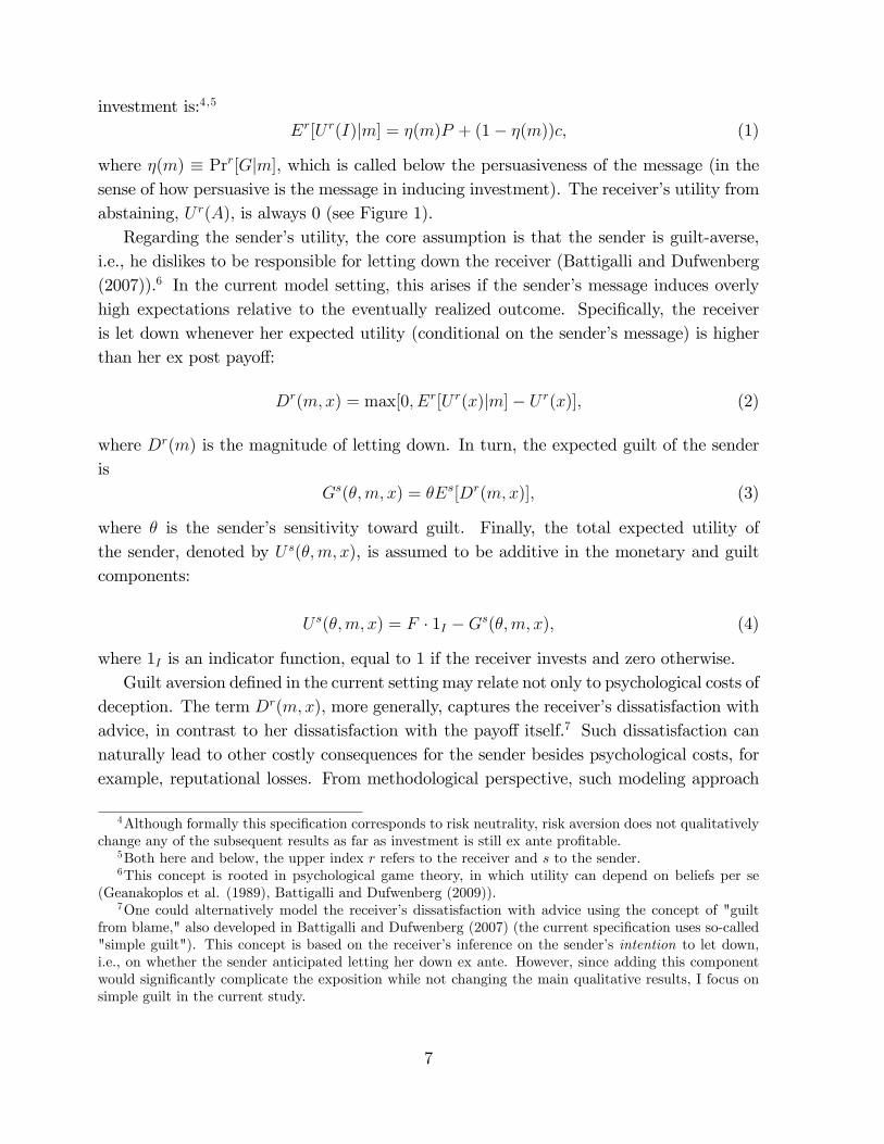
investment is:4,5

Er[U r(I)|m] = η(m)P + (1− η(m))c, (1)

where η(m) ≡ Prr[G|m], which is called below the persuasiveness of the message (in thesense of how persuasive is the message in inducing investment). The receiver’s utility fromabstaining, U r(A), is always 0 (see Figure 1).Regarding the sender’s utility, the core assumption is that the sender is guilt-averse,

i.e., he dislikes to be responsible for letting down the receiver (Battigalli and Dufwenberg(2007)).6 In the current model setting, this arises if the sender’s message induces overlyhigh expectations relative to the eventually realized outcome. Specifically, the receiveris let down whenever her expected utility (conditional on the sender’s message) is higherthan her ex post payoff:

Dr(m,x) = max[0, Er[U r(x)|m]− U r(x)], (2)

where Dr(m) is the magnitude of letting down. In turn, the expected guilt of the senderis

Gs(θ,m, x) = θEs[Dr(m,x)], (3)

where θ is the sender’s sensitivity toward guilt. Finally, the total expected utility ofthe sender, denoted by U s(θ,m, x), is assumed to be additive in the monetary and guiltcomponents:

U s(θ,m, x) = F · 1I −Gs(θ,m, x), (4)

where 1I is an indicator function, equal to 1 if the receiver invests and zero otherwise.Guilt aversion defined in the current setting may relate not only to psychological costs of

deception. The term Dr(m,x), more generally, captures the receiver’s dissatisfaction withadvice, in contrast to her dissatisfaction with the payoff itself.7 Such dissatisfaction cannaturally lead to other costly consequences for the sender besides psychological costs, forexample, reputational losses. From methodological perspective, such modeling approach

4Although formally this specification corresponds to risk neutrality, risk aversion does not qualitativelychange any of the subsequent results as far as investment is still ex ante profitable.

5Both here and below, the upper index r refers to the receiver and s to the sender.6This concept is rooted in psychological game theory, in which utility can depend on beliefs per se

(Geanakoplos et al. (1989), Battigalli and Dufwenberg (2009)).7One could alternatively model the receiver’s dissatisfaction with advice using the concept of "guilt

from blame," also developed in Battigalli and Dufwenberg (2007) (the current specification uses so-called"simple guilt"). This concept is based on the receiver’s inference on the sender’s intention to let down,i.e., on whether the sender anticipated letting her down ex ante. However, since adding this componentwould significantly complicate the exposition while not changing the main qualitative results, I focus onsimple guilt in the current study.

7

allows to make the cost of lying endogenously determined by the actual deception causedby the lie, i.e., by the deviation of the receiver’s beliefs induced by the lie from the truth.Note that Dr(m,x) = 0 if the good state is realized ex post, since the receiver cannot

be let down by the highest possible outcome (i.e., Er[U r(x)|m] ≤ P ). Consequently, thesender expects non-zero guilt given investment only if the bad state of the world is realized,which implies

U s(θ,m, I) = F − θλis(EsEr[U r(I)|m]− c), (5)

where λis is the probability of the bad state expected by the sender in state is. If the re-ceiver does not invest conditional on the message, then her outcome is no longer stochastic(being zero in all states), so that

Er(U r(A)|m) = U r(A) = 0, (6)

implyingDr(m,A) = Gs(θ,m,A) = U s(θ,m,A) = 0. (7)

Hence, the sender never expects guilt if the receiver abstains, independent of the sentmessage.8

The sender’s guilt aversion coeffi cient θ is a random variable, unknown to the re-ceiver, distributed uniformly on the interval (0, θ̄].9 This assumption serves to reflect theuncertainty of the receiver about the trustworthiness of the sender, which is widely hetero-geneous in the population, as documented by many experimental studies (e.g., Charnessand Dufwenberg (2006)). Hence, the sender type is two-dimensional: one dimension re-lates to the state of his information, while the other relates to his sensitivity to guilt (thecorresponding two-dimensional set of types is denoted by Θ).Thus, the model captures three general types of receiver uncertainty: 1) uncertainty

about the state of the world; 2) uncertainty about the state of the sender’s information;and 3) uncertainty about the sender’s trustworthiness.

2.2 Equilibrium concept

The equilibrium outcome is characterized by

8One could argue that the receiver can still be dissatisfied with advice in this case, if she finds outthat she has lost profitable investment opportunities by abstaining in the good state. At the same time,one could eliminate this type of dissatisfaction in our setting by reasonably assuming that the state ofthe world is not observable for the receiver per se(but only through the ex post payoff). For instance, thereceiver might never realize whether some innovative product fits her preferences unless she really triesthe product.

9The exclusion of 0 is purely technical and does not affect any qualitative results.

8

1. the strategy of the receiver specifying whether to invest or abstain conditional oneach possible message (ξ : M → {I, A});

2. the strategy of the sender specifying which message to send conditional on the in-formation state and the sensitivity to guilt (µ : Θ→M);

3. the receiver’s belief about the state of the world conditional on each message η(m);10

4. all higher-order beliefs about the state of the world conditional on each message.

I apply the solution concept of pure strategy perfect Bayesian equilibrium, which im-plies that the sender’s and receiver’s equilibrium strategies should maximize the respectiveexpected utility functions given equilibrium beliefs; the receiver’s first-order beliefs are de-rived by Bayes rule whenever possible; higher-order beliefs are correct (Battigalli andDufwenberg (2009)).Let us specify the optimal receiver strategy. She prefers to invest if and only if the

expected utility from investment is larger than the utility from abstaining, i.e.,11

Er[U r(I)] ≥ Er(U r(A)),

η(m)P + (1− η(m))c ≥ 0,

η(m) ≥ −cP − c ≡ η. (8)

The sender chooses the message, which maximizes his utility. Given (5) and the re-ceiver’s strategy specified above, the sender utility is

U s(θ,m, x) =

0

F − θλis(EsEr[U r(I)|m]− c)= F − θλisη(m)(P − c)

if η(m) < η,

if η(m) ≥ η,

(9)

where the equality on the RHS follows from the consistency of the sender’s second-orderbeliefs in equilibrium (i.e., EsEr[U r(I)|m] = Er[U r(I)|m] = η(m)(P − c) + c). Thus,the sender faces a tradeoff between inducing investment by being suffi ciently persuasivewith his message (to ensure η(m) ≥ η), and at the same time keeping the receiver’sexpectations low to mitigate guilt (η(m) enters negatively in the sender’s utility functiononce the receiver invests). Below, given (9), I denote the sender’s utility function asU sis(θ, η(m), x), where is is the sender’s information state.

10As becomes clear later in this subsection, the receiver’s beliefs about the state of the world are suffi cientto determine both optimal sender and receiver strategy, hence we do not need to additionally specify thereceiver’s beliefs about the sender’s type.11Hence, I assume that the receiver prefers investment over abstaining conditional on equal utility, which

precludes mixed strategies. However, analysis of equilibria with mixed strategies of the receiver does notproduce qualitatively different results.

9

The receiver’s equilibrium beliefs are determined by the sender’s messaging strategy.

Lemma 1 The persuasiveness of any equilibrium message m is

η(m) ≡ Pr[G|m] =Pr[m|G′]κ+ Pr[m|N ′](1− κ)

(Pr[m|G′] + Pr[m|B′])κ+ 2 Pr[m|N ′](1− κ).

Note that Pr[m|is] is determined by the sender’s strategy in information state is, i.e.,by the fraction of types who send the message conditional on this information state, whileκ denotes the prior probability that the sender is informed.I also impose the following restriction on out-of-equilibrium beliefs:

Assumption 2 There always exists at least one out-of-equilibrium messagem, with η(m) <

η.

This assumption can be interpreted as if there always exists an opportunity for thesender to convince the receiver not to invest. Given that the sender is monetarily bi-ased in the opposite direction, this assumption is intuitively reasonable. It rules outequilibria, when the receiver invests independently of what the sender says (including out-of-equilibrium messages). Such equilibria are economically irrelevant, since there is nointuitive reason why the receiver would then refer to the sender in the first place.12

3 Equilibrium analysis

3.1 Preliminaries

First, let us observe that in any possible equilibrium there exists a message leading toinvestment.

Lemma 2 There is no equilibrium where all messages lead to abstaining.

The intuition is that at least one equilibrium message must induce beliefs (i.e., theprobability of the good state conditional on the message) not lower than 0.5 – otherwise,there is a contradiction to the prior of 0.5. Then, the receiver should invest after thismessage by Assumption 1.Next, those types who indeed observe the good state always induce investment:

Lemma 3 In any existing equilibrium, if is = G′, then all sender types induce investment.

12The methodological advantage of this refinement is that it rules out the babbling equilibrium whenevernon-babbling equilibria exist.

10

Indeed, if the sender observes the good state, his anticipated guilt from inducing in-vestment is zero, since he knows that the receiver is not going to be let down. Hence, hisexpected utility from any message leading to investment is F , which is larger than the zeroutility from inducing abstaining. Finally, in any equilibrium, there is a possibility for thesender to send an investment-inducing message by Lemma 2.In contrast to this case, whenever the sender does not observe the good state with

certainty (i.e., is 6= G′), his expected probability of the bad state, and hence the expectedguilt from inducing investment, is strictly positive. One can show that the message strategyof such types has a cutoff structure in any equilibrium.

Lemma 4 In any existing equilibrium, for each is ∈ {B′, N ′} there exists a single cutofftype θ̂is ∈ (0, θ̄] such that all sender types with θ ≤ θ̂is send a message leading to investmentand all types with θ > θ̂is (if any) send a message leading to abstaining.

The rationale behind this result is the following. First, there are always types in anyinformation state who are suffi ciently insensitive to guilt to prefer inducing investment(which they can do by Lemma 2). Second, if some type prefers to induce investmentover getting zero from abstaining, then all less guilt-sensitive types would also preferat least the same message over zero (they would have less guilt while getting the samemonetary payoff). Analogously, once some type prefers to induce abstaining over anypossible investment-inducing message, all higher types would prefer to induce abstainingas well. This corroborates the cutoff structure described in Lemma 4.Another important distinction between different information states (besides the cutoff

structure) is that types in stateG′ have asymmetric preferences over receiver beliefs relativeto types in other states: while the former are indifferent to the persuasiveness of themessage (they do not expect to let down the receiver anyway), sender types in states B′

and N ′ always strictly prefer a less persuasive message. In the next subsections, it is shownthat such asymmetry gives rise to the possibility of separation between types in state G′ onthe one side, and types in states B′ and N ′ on the other. As a result, all existing equilibriacan be classified by the degree of this separation. I begin the equilibrium characterizationwith two extreme cases (either full or partial separation), and discuss later why only thesetwo equilibria are robust to slight perturbations in sender preferences.

3.2 Lying equilibrium

The first type of equilibrium is termed the lying equilibrium. In this equilibrium, the senderuses either the least or the most persuasive message (depending on his guilt sensitivity andinformation state), so that lying, whenever it occurs, takes an explicit form.13 In terms of

13In this section, the term "lying" is used rather informally. A formal definition of lying in our settingis given later in Subsection 4.1.

11

Figure 2: Subtypes of the lying equilibrium.

equilibrium structure, a distinctive feature of this equilibrium is that there is a completepooling of investment-inducing types in states B′ and N ′ with types in state G′.

Definition 1 The lying equilibrium is defined as an equilibrium in which

• The message mG′ is sent if θ ∈ (0, θ̄] in state G′, θ ∈ (0, θ̂l

B′ ] in state B′, and

θ ∈ (0, θ̂l

N ′ ] in state N′;

• All other types (if any) send the message mB′;

• The receiver invests after mG′, but abstains after mB′ (if used);

• The beliefs after mB′ (if used) and mG′ are determined by Bayes rule, while for anyout-of-equilibrium message m̃ it holds that η(m̃) ∈ [0, η) ∪ [η(mG′), 1]. The receiverinvests after an out-of-equilibrium message if and only if η(m̃) ≥ η.

Proposition 1 There exists a unique lying equilibrium if and only if either of the followingholds:

1. κ ≤ P+cPand F > F̃ l(κ), where F̃ l(κ) > 0 is some threshold value;

2. κ > P+cP.

Figure 2 shows possible subtypes of this equilibrium. Here, each horizontal line rep-resents the set of sender types for a given information state. The black bracket indicatestypes who use message mG′ , while the white bracket indicates types who use message mB′ .The figure shows three possible subtypes of this equilibrium depending on whether θ̂

l

N ′

and θ̂l

B′ are equal to θ̄.The basic mechanism behind this equilibrium is described as follows: In the first sub-

type of the equilibrium, the monetary sender’s incentive F is high enough such that all

12

sender types want to pool on the message mG′ , which induces investment. If the monetaryincentive decreases (Subtypes 2 and 3), then the most guilt-sensitive types in states N ′

and B′ prefer to deviate to the message mB′ , which yields abstaining and hence zero guilt(see (7)). Clearly, the fraction of such types is larger in state B′, where the expectedguilt is higher for a given sensitivity θ. No types in state G′ ever want to deviate to mB′ ,since their expected guilt is zero. Finally, no type has an incentive to deviate to out-of-equilibrium messages, which either lead to abstaining (if η(m̃) < η), or to higher guilt (ifη(m̃) ≥ η(mG′)).The equilibrium beliefs conditional on the messages mG′ and mB′ are determined by

the cutoff types θ̂l

B′ and θ̂l

N ′ (in particular, by substituting (Pr[mG′|G′] = 1, Pr[mG′ |N ′] =θ̂lN′θ̄and Pr[mG′ |B′] = θ̂

lB′θ̄into (18)). One can show that lower cutoff types imply a

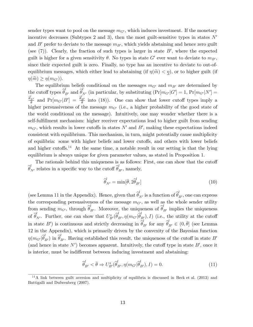
higher persuasiveness of the message mG′ (i.e., a higher probability of the good state ofthe world conditional on the message). Intuitively, one may wonder whether there is aself-fulfillment mechanism: higher receiver expectations lead to higher guilt from sendingmG′ , which results in lower cutoffs in states N ′ and B′, making these expectations indeedconsistent with equilibrium. This mechanism, in turn, might potentially cause multiplicityof equilibria: some with higher beliefs and lower cutoffs, and others with lower beliefsand higher cutoffs.14 At the same time, a notable result in our setting is that the lyingequilibrium is always unique for given parameter values, as stated in Proposition 1.The rationale behind this uniqueness is as follows: First, one can show that the cutoff

θ̂l

N ′ relates in a specific way to the cutoff θ̂l

B′ , namely,

θ̂l

N ′ = min[θ̄, 2θ̂l

B′ ] (10)

(see Lemma 11 in the Appendix). Hence, given that θ̂l

N ′ is a function of θ̂l

B′ , one can expressthe corresponding persuasiveness of the message mG′ , as well as the whole sender utilityfrom sending mG′ , through θ̂

l

B′ . Moreover, the uniqueness of θ̂l

B′ implies the uniqueness

of θ̂l

N ′ . Further, one can show that UsB′(θ̂

l

B′ , η(mG′|θ̂l

B′), I) (i.e., the utility at the cutoff

in state B′) is continuous and strictly decreasing in θ̂l

B′ for any θ̂l

B′ ∈ (0, θ̄] (see Lemma12 in the Appendix), which is primarily driven by the convexity of the Bayesian function

η(mG′|θ̂l

B′) in θ̂l

B′ . Having established this result, the uniqueness of the cutoff in state B′

(and hence in state N ′) becomes apparent. Intuitively, the cutoff type in state B′, once itis interior, must be indifferent between inducing investment and abstaining:

θ̂l

B′ < θ̄ ⇒ U sB′(θ̂

l


B′), I) = 0. (11)

14A link between guilt aversion and multiplicity of equilibria is discussed in Beck et al. (2013) andBattigalli and Dufwenberg (2007).

13

In other words, the cutoff is determined by the intersection of the function U sB′(θ̂

l

B′ , ·, I)

with the zero line. Given that U sB′(0, ·) is continuous and strictly decreasing on (0, θ̄] and

positive at 0 (U sB′(0, ·) = F > 0), such (unique) intersection exists if and only if the utility

is negative at the highest possible cutoff value:

U sB′(θ̄, η(mG′ |θ̄), I) < 0,

which is equivalent to F ≥ 0.5θ̄(P − c). Otherwise, even the most guilt-sensitive typeprefers to induce investment, and hence the only existing lying equilibrium is of Subtype1.To complete the equilibrium characterization, let us consider the receiver’s incentives.

In equilibrium, two receiver’s incentive constraints must be satisfied: η(mG′) ≥ η (so thatthe receiver prefers to invest after mG′ , see (8)), while η(mB′) < η (so that she prefers toabstain after mB′). The first requirement is always satisfied, due to the fact that all typesin state G′ pool on mG′ , which ensures η(mG′) ≥ 0.5 (while η < 0.5 by Assumption 1).Yet, the second incentive constraint η(mB′) < η can be violated if the share of uninformedtypes sending mB′ becomes suffi ciently high, which raises the persuasiveness of mB′ aboveη. This occurs when the unconditional share of uninformed types is suffi ciently high (i.e.,κ ≤ P+c

P), while the monetary incentive, and hence the cutoff in state N ′, is suffi ciently

low (i.e., F ≤ F̃ l(κ), see Proposition 1). In this case, the lying equilibrium does not exist.Let us consider the intuitive interpretation of the messages used in the lying equilibrium

(since I impose no structure on the message space, the meaning of each equilibriummessagearises endogenously). The message mG′ is always used by types who indeed observe thebest state of the world and, thus, have no incentive to downgrade information or to poolwith types in other information states. Hence, this can be interpreted as an explicit claimthat the observed state is good with certainty (in terms of exogenous formulation of themessage). Thus, the pooling of types in other information states with this message canbe interpreted as explicit lying. On the other hand, the message mB′ is used by themost guilt-sensitive types in information state B′, who would like to induce the receiverto abstain from investment. This message can thus be interpreted as an explicit claimthat the observed state was bad with certainty. Out-of-equilibrium messages m̃ can beinterpreted as being either insuffi ciently persuasive to induce investment (if η(m̃) ∈ [0, η))or overly explicit (if η(m̃) ∈ [η(mG′), 1]).Intuitively, the former group of messages can be thought to include "evasive" messages,

i.e., claims that the sender has not observed information, since this represents one ofthe actually possible information states. The fact that the receiver does not find thesemessages suffi ciently persuasive can be understood as that she believes that such messagesare rather used by types who have observed the bad state of the world and want to hidethe inconvenient truth. This reasoning is supported by the fact that types in state B′ have

14

greater disutility from guilt than types in state N ′ (conditional on the same sensitivity toguilt); consequently, they indeed have a greater incentive to send less explicit messageslike evasive ones.Note, finally, that in this equilibrium there are two types of deception that lead to a

loss of the receiver from the ex ante perspective. The first is sending the message mG′ instate B′ (deception driven by the monetary bias in sender incentives, termed as bias-drivendeception). The second type of deception is sending the message mB′ in state N ′ (or guilt-driven deception), i.e., inducing the receiver to abstain from investment by pretending toobserve the bad state of the world, while in fact not having observed any state. As discussedin Subsection 2.1, the sender does not feel guilt in this case, as he avoids any risk of lettingdown the receiver. At the same time, since investment is ex ante profitable by Assumption1, the receiver would strictly prefer to invest had she known that the sender is actuallyuninformed. Such a situation can be interpreted as an ineffi cient reluctance of the senderto recommend products that are risky though profitable from an ex ante perspective. Interms of the medical example, a doctor who is too afraid of appearing incompetent (orbeing prosecuted for bad treatment) might advise his patient to undertake only the mostconservative traditional treatments with predictable but low effi ciency, instead of tryingout more innovative (and hence, more risky), but more promising treatment methods.Analogously, a financial advisor might be reluctant to recommend reasonably risky butprofitable financial products. In such situations, promoting additional monetary incentivesfor the sender may mitigate these adverse effects; this is considered later in Subsection 4.2.

3.3 Evasion equilibrium

The second type of equilibrium in this game is the evasion equilibrium, where, besides theexplicit messages mG′ and mB′ as in the lying equilibrium, an additional evasive messagemN ′ is used. This equilibrium implies complete separation of types in state G′.

Definition 2 Evasion equilibrium is defined as an equilibrium in which

• The message mG′ is sent by all types in state G′;

• The message mN ′ is sent if θ ∈ (0, θ̂e

B′ ] in state B′, and θ ∈ (0, θ̂

e



• The receiver invests after mG′ and mN ′, but abstains after mB′ (if used);

• The beliefs after mG′, mN ′ and mB′ (if used) are determined by Bayes rule, whilefor any out-of-equilibrium message m̃ it holds that η(m̃) ∈ [0, η) ∪ [η(mN ′), 1]. Thereceiver invests after an out-of-equilibrium message if and only if η(m̃) ≥ η.

15

Figure 3: Subtypes of the evasion equilibrium.

Proposition 2 There exists a unique evasion equilibrium if and only if either of the fol-lowing holds:

1. κ ∈(0, P+c

P

]and F > F̃ e(κ), where F̃ e(κ) > 0 is some threshold value;

2. κ ∈(P+cP, 2(P+c)

2P+c

]and F ≤ θ̄ (P + c) (1−κ)

κ.

The scheme of this equilibrium is given in Figure 3. Besides types sending the highestmessagemG′ (black figure bracket) and types sending the lowest messagemB′ (white figurebracket) as in the lying equilibrium, there is a set of types using the message mN ′ (greyfigure bracket), which, as shown below, can be interpreted as an evasive message (i.e., aclaim of being uninformed).The basic mechanism is as follows: Sender types in state G′, facing no guilt, have the

same utility from both mG′ and mN ′ , which is equal to F insofar as the receiver investsafter both messages. Hence, they do not have an incentive to deviate to mN ′ . At the sametime, types in states N ′ and B′, facing a strictly positive expected guilt after bothmN ′ andmG′ , strictly prefer the evasive message, since η(mN ′) < η(mG′) (while the monetary payoffis the same). Hence, the evasive message provides a way to mitigate guilt by inducing lessoptimistic payoff expectations on the part of the receiver, while still keeping her investingafter receiving the advice. Finally, no type has an incentive to deviate to any out-of-equilibrium message m̃, which yields either abstaining and a utility of 0 (if η(m̃) ∈ [0, η))or the same monetary outcome with a higher guilt (if η(m̃) ∈ [η(mN ′), 1]).The existence and uniqueness of equilibrium cutoffs is again based on the fact that

U sB′(θ̂

e

B′ , η(mN ′|θ̂e

B′), I) is continuous and strictly decreasing in θ̂e

B′ on (0, θ̄]. Consequently,by the intermediate value theorem, given that U s

B′(0, ·) = F > 0, the unique interior cutoffθ̂e

B′ < θ̄ such that U sB′(θ̂

e

B′ , ·) = 0 exists if and only if U sB′(θ̄, ·) < 0, or equivalently,

F < θ̄ (P − c) κ− 1

κ− 2. (12)

16

In this case, the evasion equilibrium is of either Subtype 2 or Subtype 3. Otherwise, allsender types for any possible interior cutoff θ̂

e

B′ would have a strictly positive utility fromsending mN ′ , so that the only possible cutoff in state B′ (and hence in state N ′) is equalto θ̄ (Subtype 1).The receiver’s incentive constraints are η(mG′) ≥ η, η(mN ′) ≥ η and η(mB′) < η.

The first constraint is trivially satisfied. The second constraint (meaning that the evasivemessage is suffi ciently credible) is satisfied whenever the share of truly uninformed typesis suffi ciently high (i.e., κ is suffi ciently low):

κ ≤ 2(P + c)

2P + c. (13)

In addition, in Subtype 2 of the equilibrium, the only interior cutoff θ̂e

B′ should be suf-ficiently distant from the boundary θ̄ (so that there is no excessive pooling of types instate B′ pretending to be uniformed), which places additional restriction on the monetarybias F (see case 2 of Proposition 2). Finally, the constraint η(mB′) < η requires that,under suffi ciently low values of κ, F should not be too low. In this case, suffi ciently manyuninformed types prefer to induce abstaining with mB′ , which eventually increases thepersuasiveness of this message above η.Note that if P < −c (i.e., if Assumption 1 does not hold), the condition (13), which

is necessary for all three subtypes of the evasion equilibrium, never holds. The reason forthis is that the receiver will never invest after the evasive message that implies that thesender is at best uninformed, if investing conditional on no information yields an ex antenegative payoff.In the evasion equilibrium, while messages mG′ and mB′ can be interpreted in the same

way as in the lying equilibrium (claims to have observed with certainty the good and thebad states, respectively), the evasive messagemN ′ can be interpreted as a claim to have notobserved information about the state of the world. Indeed, this message is primarily sentby types who actually have not observed information (state N ′) and who have no incentiveto lie (in terms of the message formulation) insofar as they know that the receiver investsafter the message mN ′ . At the same time, types (0, θ̂

e

B′ ] in state B′ have a strict incentive

to pool with uninformed types to hide the inconvenient truth. Hence, their strategy canbe interpreted as mimicking truly uninformed types by using the same evasive message.Such evasive behavior was widely observed in the laboratory setting by Khalmetski andTirosh (2013).An important structural distinction of the evasion equilibrium relative to the lying

equilibrium is that the cutoffs in the evasion equilibrium are higher.

Lemma 5 Whenever both lying and evasion equilibria exist, for any is ∈ {B′, N ′} it holdsthat θ̂

e

is ≥ θ̂l

is with a strict inequality whenever θ̂l

is < θ̄.

17

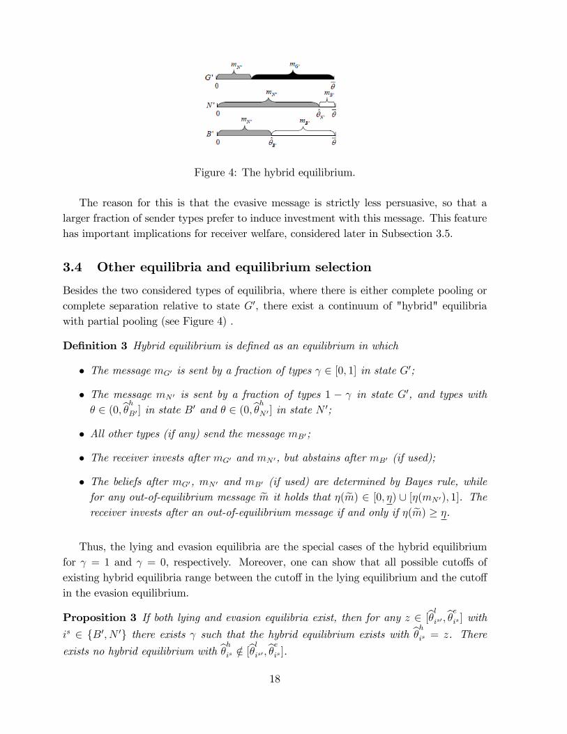
Figure 4: The hybrid equilibrium.

The reason for this is that the evasive message is strictly less persuasive, so that alarger fraction of sender types prefer to induce investment with this message. This featurehas important implications for receiver welfare, considered later in Subsection 3.5.

3.4 Other equilibria and equilibrium selection

Besides the two considered types of equilibria, where there is either complete pooling orcomplete separation relative to state G′, there exist a continuum of "hybrid" equilibriawith partial pooling (see Figure 4) .

Definition 3 Hybrid equilibrium is defined as an equilibrium in which

• The message mG′ is sent by a fraction of types γ ∈ [0, 1] in state G′;

• The message mN ′ is sent by a fraction of types 1 − γ in state G′, and types withθ ∈ (0, θ̂

h

B′ ] in state B′ and θ ∈ (0, θ̂

h



• The receiver invests after mG′ and mN ′, but abstains after mB′ (if used);

• The beliefs after mG′, mN ′ and mB′ (if used) are determined by Bayes rule, whilefor any out-of-equilibrium message m̃ it holds that η(m̃) ∈ [0, η) ∪ [η(mN ′), 1]. Thereceiver invests after an out-of-equilibrium message if and only if η(m̃) ≥ η.

Thus, the lying and evasion equilibria are the special cases of the hybrid equilibriumfor γ = 1 and γ = 0, respectively. Moreover, one can show that all possible cutoffs ofexisting hybrid equilibria range between the cutoff in the lying equilibrium and the cutoffin the evasion equilibrium.

Proposition 3 If both lying and evasion equilibria exist, then for any z ∈ [θ̂l

is′ , θ̂e

is ] with

is ∈ {B′, N ′} there exists γ such that the hybrid equilibrium exists with θ̂h

is = z. There

exists no hybrid equilibrium with θ̂h

is /∈ [θ̂l

is′ , θ̂e

is ].

18

The intuition here is that for given γ, there exist unique cutoffs in each state supportingthe equilibrium, by the same mechanism as in the lying and evasion equilibria. At the sametime, since a higher fraction of types in state G′ pooling on the message mN ′ increasesits persuasiveness and hence the associated guilt (all else equal), higher γ pushes theequilibrium cutoffs down. Since the lying equilibrium is the limit of the hybrid equilibriumif γ → 1 (complete pooling), while the evasion equilibrium is the limit if γ → 0 (completeseparation), all possible cutoffs of hybrid equilibria lie between these two cases.Although generally there also exist equilibria in this game with a different messaging

structure than in the hybrid equilibria (e.g., there can be multiple investment-inducingmessages in states N ′ and B′), the following proposition provides the reasoning for why itis suffi cient to consider only these equilibria (including the lying and evasion equilibria asspecial cases).15

Proposition 4 All existing equilibria are outcome-equivalent to the hybrid equilibria.

Inter alia, this (together with Proposition 3) implies that in any existing equilibrium,the sender cannot have higher expected guilt than in the lying equilibrium, or lower ex-pected guilt than in the evasion equilibrium. Thus, the lying equilibrium and the evasionequilibrium represent two limit cases of the whole continuum of possible equilibria in thisgame. Moreover, one can show that a simple and intuitive assumption on the sender’spreferences immediately rules out all equilibria besides the lying and evasion equilibria.

Assumption 3 There exists at least one strict lexicographic preference order in M thatis consistent with equilibrium.

Proposition 5 Under Assumption 3, there exist no other equilibria except for the lyingand evasion equilibria.

Assumption 3 implies that it is possible for the sender to strictly rank any two messageseven if they yield the same expected utility. This can be interpreted that the exogenouslygiven formulation of messages also has some value, though of infinitely small order. Thisassumption eliminates multiplicity of messages used in state G′ (a distinctive property ofthe hybrid equilibria with 0 < γ < 1), since the sender is then never indifferent betweenany two messages. Thus, all types in state G′ use the same message, so that investment-inducing types in states B′ and N ′ must either pool with all types in state G′ (the lyingequilibrium), or separate completely (the evasion equilibrium).This result justifies the focus of the subsequent analysis on only two robust equilibria,

the lying and the evasion equilibria, although the main qualitative results also remainunder consideration of the hybrid equilibria.

15The proposition can be easily extended to also cover all mixed strategy equilibria.

19

3.5 Welfare comparison

One of the key questions that can be studied with this model is whether evasion is eventu-ally detrimental from the point of view of the receiver’s welfare. In fact, from the ex anteperspective, the receiver’s utility can be both higher and lower in the evasion equilibriumthan in the lying equilibrium, depending on the monetary conflict of interest.

Proposition 6 Whenever both lying and evasion equilibria exist, the lying equilibriumyields higher ex ante utility for the receiver than the evasion equilibrium if F ≥ F ∗, anda lower utility if F < F ∗, where F ∗ is some threshold such that (1− κ) θ̄ P−c

4−3κ≤ F ∗ ≤

min[ θ̄(P+c)(1−κ)κ

, θ̄P−c4−κ ].

This result is based on the fact that the cutoff types in the evasion equilibrium arehigher (see Lemma 5). This implies that the rate of bias-driven deception (sending aninvestment-inducing message in state B′) is higher in the evasion equilibrium. Such typeof deception is clearly detrimental to the receiver’s welfare. On the other hand, the rateof guilt-driven deception (sending the message mB′ in state N ′) is higher in the lyingequilibrium. Such kind of deception is also detrimental to the receiver’s welfare, since sheprefers investment over abstaining conditional onN ′ (by Assumption 1). Thus, the sender’soption to use the evasive message in equilibrium has two effects on the receiver’s welfare.The negative effect stems from providing psychologically cheap opportunities for the senderto induce investment after observing the bad state of the world. The positive effect stemsfrom raising the effi ciency of communication of uninformed types, whose expected guilt incase of inducing investment is reduced. The total effect depends on which of these twoeffects dominates.In particular, if F is suffi ciently large (above θ̄(P − c)/(4 − κ)), then both lying and

evasion equilibria are of either Subtype 1 or Subtype 2, where there is no guilt-drivendeception (see Figures 2 and 3). Consequently, the total effect of evasion is limited toenhancing bias-driven deception in state B′, leading to a welfare loss for the receiver(when both equilibria are of Subtype 1, welfare does not change). If, to the contrary, F issuffi ciently small (below (1− κ) θ̄(P − c)/(4− 3κ)), both lying and evasion equilibria areof Subtype 3. Then, besides the negative effect, there is an additional positive effect ofevasion due to a reduction in guilt-driven deception. The clear-cut result here is that thispositive effect is always larger than the negative effect related to bias-driven deception.The reason for this is as follows. First, note that a switch from the evasion to the lyingequilibrium leads to an overall reduction of investment in states N ′ and B′ (due to thedecrease in the cutoffs). At the same time, the expected receiver’s payoff conditional onobtaining an investment-inducing message in these information states remains the same inboth equilibria. This is ensured by the fact that the ratio of the cutoffs in states N ′ and B′

is the same (see Lemmas 11 and 14 in the Appendix). Finally, this conditional expected

20

payoff is positive, because the receiver invests after mN ′ in the evasion equilibrium. Hence,the switch from the evasion to the lying equilibrium in this case effectively results (merely)in contraction of ex ante effi cient investment in states N ′ and B′, yielding a loss in welfare.Finally, one can show that if F is between the aforementioned thresholds, then the

overall effect of evasion depends on how large is the scope of guilt-driven deception in thelying equilibrium. If F is suffi ciently close to the lower threshold, guilt-driven deceptionis large enough to induce the overall positive effect of evasion. On the other hand, if F iscloser to the upper bound, then the increase in bias-driven deception due to reduced guiltin the evasion equilibrium becomes the dominant effect, making the receiver worse off inthis equilibrium. As stated in Proposition 6 there is a unique threshold F ∗ separating thetwo cases.

4 Effects of policy intervention

4.1 Prohibition of lying

In this subsection, I consider possible effects of a policy that restricts lying. The resultssuggest that under some conditions, such a policy can be detrimental to the receiver’swelfare.First, one needs a definition of lying that reflects its legal sense. Normally, lying is

understood as a misrepresentation of private information (Kartik (2009)), i.e., when astated meaning of the message deviates from the truth. As shown above, the meaning ofequilibrium messages in our model arises endogenously in both lying and evasion equilibria:mG′ (mB′) can be interpreted as a claim to have observed the good (bad) state of theworld with certainty, while mN ′ can be interpreted as a claim not to have observed anyinformation. Thus, it is reasonable to define lying in our setting as follows:

Definition 4 Lying is sending a message mis in an information state other than is, foris ∈ {G′, N ′, B′}.16

We also impose the following assumptions on verifiability:

Assumption 4 The sender’s message is (ex post) verifiable, while the sender’s informa-tion state is not.

Assumption 5 The state of the world is (ex post) verifiable if and only if the receiverinvests.

16The messages mG′ , mN ′ and mB′ themselves are implicitly defined within Definitions 1 and 2. Out-of-equilibrium messages are technically assumed to be treated as mG′ if they lead to investment, and asmB′ if they lead to abstaining.

21

Assumption 4 can be justified by the fact that the sender’s message is clearly observableto the receiver, and hence can be fixed by some communication protocol. At the sametime, in real-life applications, it is normally diffi cult to verify what information the senderactually possesses (especially, whether the sender has obtained certain information), as faras the sender obtains his information privately. Assumption 5 is justified if one thinks ofthe state of the world in terms of fitness of some advised product to the needs of a specificreceiver, which can only be verified if the receiver actually tries the product, like in thecase of medical treatment (see also footnote 7). That is, the assumption reflects the factthat it is much easier to make the sender liable for already realized losses, than for foregonepotential profits (e.g., in the case of sending mB′ in the good state of the world).17

Assumptions 4 and 5 lead to the following result.

Lemma 6 Lying is not (ex post) verifiable in the evasion equilibrium. It is verifiable inthe lying equilibrium if and only if mG′ is sent and the bad state of the world is realized.

Indeed, consider the case of sending the messagemN ′ in the evasion equilibrium. Then,by Definition 4, lying can be verified only if one could prove that the sender was in aninformation state other than N ′. At the same time, is 6= N ′ cannot be verified eitherdirectly (by Assumption 4) or by the realized state of the world, since no state of theworld excludes the possibility of having no information. In case the sender sends the lowestmessagemB′ , then in both lying and evasion equilibria, the receiver always abstains, so thatthe state of the world is not verifiable by Assumption 5. Thus, one can never prove thatthe sender has not indeed observed the bad state. Finally, if mG′ is sent and the good stateof the world is realized, the only possible case of lying in this case – sending mG′ whilebeing uninformed in the lying equilibrium – cannot be distinguished from truth-tellingeither. The only possible case where lying is verifiable is when the message mG′ is sentand the bad state of the world is realized (this is possible only in the lying equilibrium).Then, the information state G′ can be excluded with certainty since Pr[G′|σ = B] = 0.Next, consider the effect of a policy intervention such that a suffi ciently high fine is

introduced for any verifiable lying. Lemma 6 then implies that incentives in the evasionequilibrium are not affected by the policy. Yet, if the fine is suffi ciently high, then thelying equilibrium is no longer possible: no types in information states N ′ and B′ wouldthen prefer to send mG′ , given that the ex ante probability of the bad state of the world(revealing lying) in these information states is positive. Besides, the policy interventionrenders a new possible equilibrium, termed the ’evasive babbling equilibrium.’ This isdefined as an equilibrium where all types in state B′ pool with all types in state N ′

17Note that the main qualitative result of this subsection (that a lying prohibition policy reduces exante welfare in certain cases) also holds without Assumption 5, which is introduced rather for simplicityof exposition.

22

by sending the evasive message mN ′ , which effectively induces the receiver to abstainconditional on this message.

Definition 5 Evasive babbling equilibrium is defined as an equilibrium in which:

• The message mG′ is sent by all types in state G′;

• The message mN ′ is sent by all types in state B′ and all types in state N ′;

• The receiver invests after mG′, but abstains after mN ′;

• The beliefs after mG′, and mN ′ are determined by Bayes rule. For the out-of-equilibrium message mB′ it holds that η(mB′) ∈ [0, η) while the receiver abstains.

Under a suffi ciently high fine for lying, this indeed constitutes an equilibrium. As before,no types in state G′ would like to deviate to a message that leads to abstaining. Besides,no types in states N ′ and B′ would like to deviate to mG′ , while this would lead to apositive probability of being fined ex post. Deviation to the out-of-equilibrium messagemB′ does not make the sender better off either, as the receiver still abstains. Finally, thereceiver invests after mG′ and abstains after mN ′ insofar as the persuasiveness of mN ′ issuffi ciently low, i.e., η(mN ′) < η. One can show that this holds whenever κ > P+c

P(i.e., the

share of truly uninformed types is suffi ciently low). The following proposition summarizesthe equilibrium characterization under the policy intervention.

Proposition 7 If lying is prohibited, then:

• There exists an evasion equilibrium under the same parameter restrictions as before;

• There exists an evasive babbling equilibrium if and only if κ > P+cP;

• No other equilibria exist.

Let us now consider how the policy intervention changes the equilibria and receiverwelfare relative to the pre-policy status quo. Since the policy does not distort incentives inthe evasion equilibrium, I assume that the pre-policy equilibrium is the lying equilibrium(otherwise the policy-maker would not have strict incentives to implement the policy).Besides, to make the results easier to represent, I assume that the evasive babbling equi-librium does not emerge if the (more informative) evasion equilibrium is possible instead.The following proposition summarizes the findings regarding welfare implications of thepolicy intervention:

Proposition 8 If the initial equilibrium is the lying equilibrium, then the prohibition oflying results in either of the following:

23

Figure 5: The effect of lying prohibition in the case of constructive evasion.

• Switch to the evasion equilibrium if κ ≤ P+cP, or κ ∈

(P+cP, 2(P+c)

2P+c

]and F ≤

θ̄ (P + c) (1−κ)κ

(case of constructive evasion):

—Decrease in the receiver’s welfare if F ≥ F ∗, and increase otherwise.

• Switch to the evasive babbling equilibrium if κ ∈(P+cP, 2(P+c)

2P+c

]and F > θ̄ (P + c) (1−κ)

κ,

or κ > 2(P+c)2P+c

(case of destructive evasion):

—Decrease in the receiver’s welfare if κ ≤ 2(P+c)2P+c

and F ≤ (P 2−c2)(1−κ)θ̄(P (1−κ)−c)κ , increase

otherwise.

Let us consider these cases. If there is a switch from the lying to the evasion equilibrium(constructive evasion case), then all welfare implications given by Proposition 6 are in place(Figure 5). That is, if the monetary conflict of interest is high enough so that guilt-drivendeception is negligible, the equilibrium switch as a result of the policy has a net negativeeffect due to an increase in bias-driven deception. At the same time, under a low conflictof interest (or, equivalently, relatively high guilt aversion), the policy has a positive effectdue to reduction in guilt-driven deception. Note that lying prohibition policy is naturallymotivated by high conflict of interest between experts and consumers on the market, so thatthe first case (characterized by decrease in welfare) may be considered more economicallyrelevant.Note that to induce a switch to the evasion equilibrium (in terms of real-world applica-

tions), the policy should not only prohibit verifiable lying, but also be accompanied by an

24

Figure 6: The effect of lying prohibition in the case of destructive evasion.

increase in trust in the evasive message mN ′ . Indeed, the lying equilibrium always hingeson low out-of-equilibrium beliefs regarding mN ′ (i.e., the receiver interprets this messagerather as concealing unfavorable information). Yet, there is an intuitive interpretationas to why these beliefs can be higher after the policy intervention: it becomes commonknowledge that evasion is the only possible way to induce investment for a truly uninformedsender, since explicit lying is not possible any longer. This might increase the receiver’strust in the evasive message, hence leading to emergence of the evasion equilibrium.The other scenario is when the policy induces a switch from the lying to the evasive

babbling equilibrium (the case of destructive evasion, Figure 6). This effectively destroysall investment, which takes place in the lying equilibrium conditional on is 6= G′. Whetherthis has a net positive effect for the receiver depends on the quality of such investment,i.e., on the relative shares of types in states N ′ and B′, inducing investment in the lyingequilibrium. The relative share of types in state N ′ is suffi ciently high if, first, the priorprobability of being uninformed is relatively high (κ ≤ 2(P+c)

2P+c), and second, the conflict

of interest is relatively low (so that suffi ciently many types in state B′ do not induceinvestment by sending mB′). In this case, investment in the lying equilibrium conditionalon is 6= G′ yields an ex ante positive payoff for the receiver. Abandoning such investmentdue to destruction of any persuasive communication in states N ′ and B′, which happensin the evasive babbling equilibrium, leads to a net welfare loss for the receiver. In otherwords, the lying prohibition policy may lead to excessive evasion of types in state B′,resulting in destruction of any effi cient communication from uncertain senders.Thus, policy aimed at lying prohibition can be welfare enhancing in several cases. First,

if most of sender types are informed about the true state of the world, then lying prohibi-tion basically eliminates deception of types who have observed the bad state (Scenario 2,positive case). Second, if there is too much of ineffi cient precaution of uninformed senderson the market (guilt-driven deception), then enhancing credible evasive communication asa result of the policy can serve as a way to reduce such precaution (Scenario 1, positivecase). At the same time, if the precaution is not an issue and, besides, there is a suffi -ciently high share of uninformed senders on the market, then a prohibition of lying canlead to a spread of deception in the form of evasive communication (Scenario 1, negative

25

case). Finally, pooling with types observing the good state of the world can be the onlyway to induce investment for uncertain senders. Eliminating this possibility due to lyingprohibition can also lead to a net welfare loss (Scenario 2, negative case). Importantly,the cases where lying prohibition leads to welfare loss are attributed to the effect of guiltaversion, and cannot be explained by outcome-based preferences (see Section 6 below).In summary, although the receiver does not like lying per se, she might prefer to have

lying on the equilibrium path, as it then serves as a disciplining device for guilt-aversesenders. In this sense, lying, as a population phenomenon, can be interpreted to have a"hidden value," which can be destroyed by an overly interventionist policy.

4.2 Regulation of commission payments

Let us consider the case where the regulator mitigates the conflict of interest between thesender and the receiver by capping the sender’s contingent payment F . One can showthat such policy can backfire by making the sender’s guilt motivation too prominent, inparticular, for uninformed sender types. This can lead to foregone investment opportunitiesas a result of overly precautionary advice from uninformed types (guilt-driven deception).At the same time, the policy also works positively by inducing more truth-telling amongtypes observing the bad state of the world, i.e., by reducing bias-driven deception. Thefollowing proposition summarizes the total effect.

Proposition 9 Welfare strictly increases with F if κ < 2(P+c)2P+c

and:

• F < (P−c)4−κ θ̄ in the lying equilibrium;

• F < (P−c)(1−κ)4−3κ

θ̄ in the evasion equilibrium.

Otherwise, welfare decreases with F .

Thus, a higher bias in the sender’s monetary incentives has a net positive effect on thereceiver’s welfare if κ and F are suffi ciently small. In this case, there is a suffi ciently largeshare of uninformed senders (due to small κ), who are involved in guilt-driven deception(due to small F ). Thus, higher bias works positively due to reducing this kind of deception.In fact, whenever there is any guilt-driven deception while the evasion equilibrium exists,higher F has a net positive effect on welfare (see Subsection 3.5). Thus, biased incentivesof the sender may be eventually beneficial to the receiver, insofar as they help to mitigateexcessive precaution of the sender (see also the discussion at the end of Subsection 3.2).One can demonstrate another notable result regarding the effect of complete elimination

of the monetary conflict of interest, i.e., setting F = 0. For example, this can correspondto banning of commissions for financial advisors, which has been recently undertaken

26

in the UK, as noted in the Introduction. It follows from Proposition 9 that F = 0 isalways suboptimal as far as either lying or evasion equilibrium exists. At the same time,Propositions 1 and 2 suggest that these equilibria exist for F = 0 only if κ > P+c

P. To

obtain an equilibrium prediction for the case if κ ≤ P+cP(i.e., the share of uninformed

sender types is suffi ciently high), let us lift Assumption 2.18 Then, one can show thatsetting F = 0 may lead to a welfare loss also through a reversal to babbling equilibrium.

Proposition 10 If κ ≤ P+cPthen setting F = 0 leads to either the evasion or the lying

equilibrium of Subtype 1 and to a lowest possible ex ante receiver welfare.

Indeed, if κ ≤ P+cP, i.e., the unconditional share of uninformed sender types is suffi -

ciently high, no informative equilibria are incentive-compatible as far as F = 0. The reasonfor this is that the receiver prefers to invest even after the lowest message mB′ : then, toomany truly uninformed sender types try to induce abstaining with mB′ (see Subsections3.2 and 3.3). In this case, the only possible equilibria are when the receiver invests afterany message, i.e., either the lying or the evasion equilibrium of Subtype 1. Since Assump-tion 2 is lifted, one could then allow for out-of-equilibrium messages that do not lead toabstaining (or to a lower guilt), thus making the sender’s strategy consistent with theseequilibria. Since the advice is completely uninformative in this case, the receiver has thelowest possible ex ante payoff in comparison to any other equilibria, which are possiblewith higher F .Thus, eliminating the sender’s monetary interest in recommending risky options for

the receiver may sometimes lead to excessive downgrading of information by senders whoare not certain of the eventual outcome, inducing a reversal to a babbling equilibrium and,consequently, a welfare loss.

5 Effect of quality of the sender’s information

The parameter κ in our model setting, denoting the probability that the sender is informed,can also be interpreted as the quality of the sender’s information (or the strength of hisexpertise). Indeed, κ effectively denotes the ex ante probability that the sender’s privateinformation is relevant for a particular receiver (i.e., it can be used to predict the outcomesof her available decision options). Hence, higher κ can mean that the sender’s privateinformation is of higher quality (or that his expertise is higher).Common intuition suggests that once the receiver is rational, and thus cannot be made

worse off by communication with the sender, she should benefit from a higher quality of

18The assumption is not critical for all the previous results and helps only to eliminate multiplicityof equilibria: Without this assumption, the babbling lying and evasion equilibria of Subtype 1 are alsopossible whenever non-babbling equilibria exist.

27

the sender’s information. However, as shown below, this is not always the case due to theeffect of the sender’s guilt aversion. The following proposition summarizes the results.

Proposition 11 i) In the lying equilibrium, U r,l is U-shaped in κ if

θ̄P − c4− κ > F > θ̄

(P − c)2

2(3P + c)

and increasing in κ otherwise.ii) In the evasion equilibrium, U r,e is strictly decreasing in κ if

θ̄(1− κ)(P − c)2− κ > F > max[

θ̄(1− κ)(P − c)1 +√

1 + κ2,θ̄(1− κ)(P − c)

4− 3κ]

and increasing in κ otherwise.

Consider the lying equilibrium. There, an increase in κ has two effects: a direct positiveand an indirect negative. The positive effect relates to the fact that once the sender isinformed (i.e., is either in state G′ or B′) the receiver is more likely to invest in the goodthan in the bad state of the world. The reason for this is that the share of types inducinginvestment in state B′ is lower than such share in state G′ (unless the equilibrium is ofSubtype 1 where these are equal). On the other hand, if the sender is uninformed, thenthe receiver is equally likely to invest in both states of the world. Moreover, there can beforegone investment in the good state of the world (due to guilt-driven deception), whichnever happens with an informed sender. Altogether, this implies that

E[U r,l|G′ ∨B′] ≥ E[U r,l|N ′], (14)

so that an increase in κ and, hence, the probability of facing an informed sender has apositive effect on welfare (all else equal). The magnitude of this effect depends on themonetary conflict of interest. If F becomes smaller, then the rate of bias-driven deceptionof informed sender types decreases, which makes the advice of informed types relativelymore effi cient. This effect of smaller F is intensified even more by an additional increasein guilt-driven deception of uninformed sender types.However, an increase in κ also has an indirect negative effect on welfare through guilt

aversion. In particular, higher κ implies that the message mG′ is more likely to be sent byinformed types, which by (14) should lead to a higher expected receiver’s utility conditionalon the message (all else equal). This results in higher expected guilt of the sender fromsending mG′ , pushing the cutoff types down. In particular, if the equilibrium is of Subtype3, which occurs if F < θ̄(P−c)

(4−κ), the cutoff θ̂

l

N ′ is then interior so that it strictly decreasesin response to an increase in κ. This leads to an increase in guilt-driven deception of

28

uninformed sender types, which results in a welfare loss for the receiver (especially, if thefraction of these types is high, i.e. for low values of κ). This negative effect dominates thedirect positive effect if the latter is low, which happens if F is relatively high (in particular,if F > θ̄ (P−c)2

2(3P+c)), as discussed in the preceding paragraph.

In the evasion equilibrium, an increase in κ again has two effects. The first (positive)effect is the same as in the previous case: the receiver prefers (from the ex ante perspective)to deal with an informed rather than an uninformed sender. The second (negative) effectis driven by guilt aversion: higher κ decreases the persuasiveness of the evasive messagemN ′ (in contrast to the case of the lying equilibrium, where the persuasiveness of mG′ isincreasing with κ). In particular, higher κ implies that the share of truly uninformed typesis lower such that the evasive message mN ′ rather signals types in state B′ who want toconceal their bad news. By being less persuasive, the message mN ′ induces less guilt onthe part of the sender such that the equilibrium cutoffs increase. If the equilibrium is ofSubtype 2, then the resulting welfare effect is negative, due to the spread of bias-drivendeception. This effect dominates the direct positive effect if F is high enough (but not toohigh such that the equilibrium is of Subtype 1 and the cutoffs are constant at θ̄) for thesame reasons as in the case of the lying equilibrium.Thus, the ex ante likelihood of obtaining the informative signal affects the sender’s

anticipation of guilt, and hence the rate of truth-telling conditional on a given informationstate. This mechanism leads to seemingly paradoxical cases where even a completelyrational receiver prefers to deal with the sender, who is less likely to have the informationshe needs.19

6 Comparison to outcome-based models

One may ask whether the obtained results are attributable to belief-dependent preferences,and cannot be derived with a simpler model based only on outcome-based preferences.To address this question, let us assume that the sender cares solely about his and thereceiver’s monetary outcomes. In particular, the sender has some fixed cost ψ of incurringthe receiver’s losses (e.g., arising from inequity aversion (Bolton and Ockenfels (2000) andFehr and Schmidt (1999))), which he bears if the receiver gets a negative payoff of c. Forsimplicity, I assume that the sender has no change in utility if the receiver gets 0 or B,although the subsequent results are easily generalizable if one assumes the opposite.20

Then, the sender’s utility conditional on investment, denoted by U s,0, can be represented

19A positive effect of noise in the sender’s information (through a different mechanism than con-sidered here) is also found by Blume et al. (2007) within the benchmark cheap-talk framework ofCrawford and Sobel (1982).20The only assumption that matters here is that the sender’s utility does not directly depend on beliefs.

29

in the following form:U s,0(θ, I) = F − Pr[B] · θψ, (15)

where θ is the sensitivity parameter, distributed uniformly as above on (0, θ̄]. Conditionalon abstaining, we have

U s,0(θ, A) = 0. (16)

It is then straightforward to show that the equilibrium in this model also has a cutoffstructure. The cutoff type, once interior, must be indifferent between investment andabstaining:

F − Pr[B|is] · θ̂0

isψ = 0,

θ̂0

is =F

Pr[B|is]ψ. (17)

Importantly, no evasion emerges once the sender has even infinitely small preferencesover message formulations (i.e., under Assumption 3).

Proposition 12 Under the outcome-based preferences, the only possible equilibrium is thelying equilibrium, which exists if and only if either of the following holds:

1. κ ≤ P+cPand F > F̃ h(κ), where F̃ h(κ) > 0 is some threshold value;

2. κ > P+cP.

Indeed, in the evasion equilibrium, an outcome-concerned sender would have the sameutility from both investment-inducing messages (mN ′ and mG′), because the receiver’s ac-tion (investment), and hence the expected monetary outcomes of both players conditionalon these messages are the same. Then, the sender would deviate to the message, whichis strictly preferred in lexicographic preference order by Assumption 3. Still, even in theabsence of this assumption, the evasion equilibrium, though possible, cannot be consideredrobust, since the sender types in states B′ and N ′ do not have a strict incentive to separatefrom the types in state G′, unlike in the main model. Hence, the endogenous emergenceof evasive communication is robust only with belief-dependent preferences.Let us consider whether the lying prohibition policy in the outcome-based model has

the same welfare effects as those considered in Subsection 4.1. Once verifiable lying (i.e.,pooling with types in state G′) is prohibited, the evasion equilibrium becomes possible,since no types in state B′ and N ′ would like to deviate to mG′ under a suffi ciently highfine. Besides, there also exists the evasive babbling equilibrium if and only if κ > P+c

P(as

above). Thus, the policy also results in a switch from the lying to either the evasion or theevasive babbling equilibrium. However, the welfare effect of this switch is very differentfrom the one in the main model.

30

Proposition 13 Under the outcome-based preferences, prohibition of lying never resultsin a decrease in welfare.

Intuitively, welfare does not change if there is a switch from the lying to the evasionequilibrium. The reason for this is that the cutoffs (and hence the ex ante investmenteffi ciency) are the same in both equilibria, since they do not depend on beliefs induced bythe messages, but only on their monetary consequences (see (17)). In the other possiblescenario, if there is a switch to the evasive babbling equilibrium (whenever the evasionequilibrium cannot emerge), welfare always increases. This is because, if investment con-ditional on is 6= G′ is ex-ante ineffi cient in the (candidate) evasion equilibrium (while itdoes not exist), such investment must be also ineffi cient in the lying equilibrium with thesame cutoffs. Since a switch from the lying to the evasive babbling equilibrium eliminatesthis case of investment, welfare increases.Regarding other results, one can show that, in the outcome-based model, reducing or

banning commissions may also have negative welfare effects due to the resulting ineffi cientprecaution of uninformed sender types. There can also be a switch to the babbling equilib-rium if commissions are eliminated, similar to Proposition 10.21 However, the result thatthe receiver’s welfare can decline with the quality of the sender’s private signal cannot beexplained by outcome-based preferences.

Proposition 14 Under outcome-based preferences, the welfare never decreases with κ.

The reason for this is that now the increase in κ does not affect the sender’s utilityfrom inducing investment, and hence the equilibrium cutoffs and the rate of deception ineach state. Consequently, the only result of such increase is that the receiver is more likelyto obtain more ex ante effi cient advice from an informed sender.Thus, outcome-based preferences cannot explain a possible decrease in welfare due to

the lying prohibition or making the sender’s signal more (ex ante) precise, which is drivenexclusively by guilt aversion.

7 Conclusion

This paper studies a model of strategic communication where the sender’s cost of lying isendogenously determined by the receiver’s beliefs. One of the main results is that suchpreferences can lead to the endogenous emergence of evasive communication in equilibrium(i.e., downgrading the quality of obtained information), which helps to avoid guilt frombiasing the receiver’s expectations. At the same time, there also exists an alternative

21Since the arguments are similar to the main case, I do not formalize them here.

31

equilibrium where only explicit communication is used, precluding any meaningful evasivemessages and, thus, disciplining guilt-sensitive senders. A policy aimed at lying prohibitionmay induce a switch from explicit to evasive communication, which can have both negativeand positive welfare consequences. A negative effect occurs since the deception is lesspsychologically costly once it takes the form of evasive messages, while a positive effectis related to enhancing communication for truly uncertain senders. The net effect can beboth positive and negative, depending on the precision of the sender’s information and hismonetary preference bias.Our analysis also reveals that higher (ex-ante) precision of the sender’s private informa-

tion can harm the receiver in certain cases. In particular, this can occur due to the reducedcredibility of evasive messages and hence the associated guilt, which leads to expanded useof these messages to conceal bad news. Finally, monetary commissions for the advisor cansometimes play a role of compensation for risk, which the caring advisor faces while beinguncertain about the suitability of his advice. Hence, banning such commissions can resultin an ineffi cient degree of precaution by providing advice.The analysis generally suggests that policies aimed at restriction of experts’lying or

their conflict of interest with consumers should be applied with caution. In certain cases,such policies can backfire by interfering with otherwise effi cient self-regulatory mechanisms,which are based on the intrinsic and natural motivation of experts to provide good adviceto their clients.

Appendix: Omitted Proofs

Proof of Lemma 1. We have

η(m) ≡ Pr[G|m] =Pr[m|G] Pr[G]

Pr[m]

=(Pr[m|G′ ∩G] Pr[G′|G] + Pr[m|N ′ ∩G] Pr[N ′|G]) Pr[G]

Pr[m|G′] Pr[G′] + Pr[m|N ′] Pr[N ′] + Pr[m|B′] Pr[B′]

=(Pr[m|G′] Pr[G′|G] + Pr[m|N ′] Pr[N ′|G]) Pr[G]

Pr[m|G′] Pr[G′] + Pr[m|N ′] Pr[N ′] + Pr[m|B′] Pr[B′]

=Pr[m|G′]κ+ Pr[m|N ′](1− κ)

(Pr[m|G′] + Pr[m|B′])κ+ 2 Pr[m|N ′](1− κ), (18)

where the second equality is by Bayes rule, the third equality is by the law of total proba-bility, and the fourth equality is by the fact that equilibrium messages of any sender typeθ are contingent on his information state is, but not on the true state of the world (by thedefinition of equilibrium in Subsection 2.2), i.e., Pr[m|is ∩G] = Pr[m|is] for any is.

Proof of Lemma 2. Assume by contradiction that all messages used on the equilibrium

32

path induce conditional beliefs lower than η (so that the receiver abstains after all of them,see (8)), i.e.,

∀m ∈ ΥE,Pr[G|m] < η, (19)

where ΥE is the union set of all messages used in equilibrium. By Bayes rule,

Pr[G|ΥE] =Pr[ΥE|G] Pr[G]

Pr[ΥE]= Pr[G] = 0.5, (20)

since Pr[¬ΥE|G] = Pr[¬ΥE] = 0 (by definition of ΥE) so that Pr[ΥE|G] = Pr[ΥE] = 1.At the same time, since messages are mutually exclusive events,

Pr[ΥE|G] =∑m∈ΥE

Pr[m|G] =∑m∈ΥE

Pr[G|m] Pr[m]

Pr[G], (21)

where the last equality is by Bayes rule. Substituting (21) and Pr[ΥE] = 1 into (20) weobtain

Pr[G|ΥE] =Pr[ΥE|G] Pr[G]

Pr[ΥE]

=

∑m∈ΥE

Pr[G|m] Pr[m]Pr[G]

Pr[G]

1=∑m∈ΥE

Pr[G|m] Pr[m]

<∑m∈ΥE

η Pr[m] = η∑m∈ΥE

Pr[m] = η =−cP − c < 0.5, (22)

where the first inequality is by (19) and the second one is by Assumption 1. Since (22)contradicts (20), the claim follows.

Lemma 7 A necessary condition for the existence of equilibrium is that the persuasivenessof any investment-inducing message used in states is ∈ {B′, N ′} is the same.

Proof. Assume by contradiction that there exist two investment-inducing messages m1

and m2 sent in at least some of the information states is ∈ {B′, N ′} such that η(m1) >

η(m2). Then, any type θ would strictly prefer m2 over m1 in any information state is ∈{B′, N ′} since as far as is 6= G′ (so that λis > 0) we have

U sis(θ, η(m1), I) = F − θλisη(m1)(P − c) < F − θλisη(m2)(P − c) = U s

is(θ, η(m2), I). (23)

Thus, m1 cannot be an equilibrium message.

Proof of Lemma 3. Assume by contradiction that some sender type in state G′ sendsa message leading to abstaining, so that his expected utility from sending this message is

33

0 (by (7)). At the same time, by Lemma 2 there exists at least one message m′ leadingto investment. By (9), the expected utility from sending this message for the consideredsender type is

U s(θ,m′, I) = F − θλG′η(m)(P − c) = F > 0, (24)

where the second equality follows from the fact that λG′ = Pr[B|G′] = 0. Consequently,the sender would have a strict incentive to deviate to m′, which yields a contradiction.

Proof of Lemma 4. Assume that equilibrium exists. By Lemma 2 there exists at leastone message m′ leading to investment. Then, there always exists suffi ciently small θ̃ suchthat

U sis(θ̃, η(m′), I) = F − θ̃λisη(m′)(P − c) ≥ 0 = U s

is(θ̃, ·, A), (25)

where the first equality is by (9), and the second by (7). Thus, in any equilibrium at leastsome types in states is 6= G′ must prefer an investment-inducing message.Next, by Lemma 7 all messages used by types in states B′ and N ′ have the same per-

suasiveness, which I denote by η′. Consider further the following possible cases dependingon the utility of the most guilt sensitive type in some state is ∈ {B′, N ′}.Case 1: U s

is(θ̄, η′, I) ≥ 0. In this case, type θ̄ prefers to induce investment over ab-

staining (since the latter action yields zero utility). Then, since U sis(θ, η, I) is continuously

decreasing in θ for given η, it follows that for all θ < θ̄ it holds

U sis(θ, η

′, I) > 0, (26)

that is all these types should induce investment in equilibrium as well.Case 2: U s

is(θ̄, η′, I) < 0. In this case, since at the same time U s

is(0, η′, I) = F > 0, by

the intermediate value theorem there must exist type θ̂is ∈ (0, θ̄) such that

U sis(θ̂is , η

′, I) = 0. (27)

Then, for all θ ≤ θ̂is it holds U sis(θ, η

′, I) ≥ 0 (so that these types prefer to induce invest-ment), while for all θ > θ̂is it holds U s

is(θ, η′, I) < 0 (so that these types prefer to induce

abstaining). Finally, in the considered case there must be at least one message leading toabstaining in equilibrium so that the types θ > θ̂is can choose this message. Otherwise,these types would have a strict incentive to deviate to an out-of-equilibrium message lead-ing to abstaining and get 0 instead of a negative utility (such out-of-equilibrium messagesexist by Assumption 2).Hence, in all possible cases, if there exists an equilibrium, then it must have the cutoff

structure described in the lemma.

Lemma 8 A necessary condition for the existence of equilibrium is θ̂N ′ ≥ θ̂B′ .

34

Proof. Assume by contradiction that there exists an equilibrium such that

θ̂N ′ < θ̂B′ . (28)

Then, all types in the interval (θ̂N ′ , θ̂B′) induce abstaining in state N ′ and induce invest-ment in state B′. Consequently, these types have a negative utility from any investment-inducing message in state N ′ (otherwise they would deviate to such message from inducingabstaining, which yields the utility of 0), and a positive utility from inducing investmentin state B′ (otherwise, they would deviate to inducing abstaining). Hence, for any θ′ ∈(θ̂N ′ , θ̂B′) it holds

U sN ′(θ

′, η̂, I) < 0 ≤ U sB′(θ

′, η̂, I), (29)

where η̂ is the persuasiveness of investment-inducing messages in states is ∈ {B′, N ′}(unique by Lemma 7). At the same time, for any θ ∈ (0, θ̄] it holds (given (9))

U sB′(θ, η̂, I) = F − θη̂(P − c) < F − 0.5θη̂(P − c) = U s

N ′(θ, η̂, I), (30)

which yields a contradiction to (29).

Lemma 9 A necessary condition for the existence of equilibrium is that either θ̂is < θ̄ andU sis(θ̂is , η(m(θ̂is)), I) = 0 or θ̂is = θ̄ and U s

is(θ̂is , η(m(θ̂is)), I) ≥ 0.

Proof. Denote by η̂ the persuasiveness of investment-inducing messages in states is ∈{B′, N ′} (unique by Lemma 7). Assume by contradiction that equilibrium exists andeither θ̂is < θ̄ and U s

is(θ̂is , η̂, I) 6= 0 or θ̂is = θ̄ and U sis(θ̂is , η̂, I) < 0 for some is ∈ {B′, N ′}.

Let us demonstrate a contradiction in each of these cases separately.

Case 1: θ̂is < θ̄ and U sis(θ̂is , η̂, I) 6= 0.

First, let us consider the case U sis(θ̂is , η̂, I) > 0. Then, since U s

is(θ̂is , η̂, I) is continuouslydecreasing in the first argument (see (9)), there would exist types suffi ciently close to θ̂issuch that θ > θ̂is and U s

is(θ, η̂, I) > 0. At the same time, according to Lemma 4 suchtypes induce abstaining and get the utility of 0, so that they would have a strict incen-tive to deviate to an investment-inducing message yielding the positive utility U s

is(θ, η̂, I).Analogously, if U s

is(θ̂is , η̂, I) < 0, then types suffi ciently close to θ̂is on the left have a neg-ative utility from inducing investment and hence a strict incentive to deviate to inducingabstaining. We have come to contradiction in all possible cases.

Case 2: θ̂is = θ̄ and U sis(θ̂is , η̂, I) < 0.

Then, analogously to the previous case, there would exist types θ such that θ < θ̂is andU sis(θ, η̂, I) < 0, which then would like to deviate at least to an out-of-equilibrium messageleading to abstaining (existing by Assumption 2) that yields a contradiction.

35

Lemma 10 A necessary condition for the existence of equilibrium is θ̂N ′ = min[θ̄, 2θ̂B′ ].

Proof. Denote by η̂ the persuasiveness of investment-inducing messages in states is ∈{B′, N ′} (unique by Lemma 7). Assume by contradiction that equilibrium exists andθ̂N ′ 6= min[θ̄, 2θ̂B′ ]. Let us consider two possible cases θ̂N ′ < θ̄ and θ̂N ′ = θ̄.

Case 1: θ̂N ′ < θ̄. By Lemma 8 it then follows θ̂B′ < θ̄. Consequently, by Lemma 9 andequation (9) we have

U sB′(θ̂B′ , η̂, I) = F − θ̂B′ η̂(P − c) = 0, (31)

U sN ′(θ̂N ′ , η̂, I) = F − 0.5θ̂N ′ η̂(P − c) = 0. (32)

This implies

θ̂B′ =F

η̂(P − c) , (33)

θ̂N ′ =F

0.5η̂(P − c) , (34)

and, consequently,θ̂N ′ = 2θ̂B′ . (35)

This, together with θ̂N ′ < θ̄, implies min[θ̄, 2θ̂B′ ] = 2θ̂B′ , which finally yields a contradic-tion to θ̂N ′ 6= min[θ̄, 2θ̂B′ ].

Case 2: θ̂N ′ = θ̄. Since we have also assumed θ̂N ′ 6= min[θ̄, 2θ̂B′ ], this implies

θ̄ 6= min[θ̄, 2θ̂B′ ] (36)

⇒ θ̂B′ < 0.5θ̄. (37)

Next, we have

U sB′(0.5θ̄, η̂, I) = F − 0.5θ̄η̂(P − c)

= U sN ′(θ̄, η̂, I) ≥ 0, (38)

where the last inequality holds due to θ̂N ′ = θ̄ and Lemma 9. Consequently, for anyθ < 0.5θ̄ it holds U s

B′(θ, η̂, I) > 0 so that all types with θ < 0.5θ̄ should strictly prefer toinduce investment, contradicting to (37).

Lemma 11 If the strategies and beliefs are specified according to Definition 1, then thesender has no incentives to deviate if and only if the following two conditions hold:1) either θ̂

l

B′ < θ̄ and U sB′(θ̂

l

B′ , η(mG′), I) = 0 or θ̂l

B′ = θ̄ and U sB′(θ̂

l

B′ , η(mG′), I) ≥ 0.

2) θ̂l

N ′ = min[θ̄, 2θ̂l

B′ ].

36

Proof. The necessity of the both conditions follows by Lemmas 9 and 10. Let us considertheir suffi ciency and assume that both conditions hold. First, no type in state G′ has anincentive to deviate to mB′ , while his utility from investment is always strictly positive(see (24)). Second, it is straightforward to show that, once the first condition holds, notype in state B′ has a strict incentive to deviate to another equilibrium message given thatU sB′(θ̂

l

B′ , η(mG′), I) is continuously decreasing in its first argument.Let us show that all types in state N ′ also do not have incentives to deviate to another

equilibrium message. Consider the following possible cases.

Case 1: θ̂l

B′ < 0.5θ̄. Then, by assumption, θ̂l

N ′ = 2θ̂l

B′ < θ̄. Hence,

U sN ′(θ̂

l

N ′ , η(mG′), I) = U sN ′(2θ̂

l

B′ , η(mG′), I)

= F − 0.5 · 2θ̂l

B′η(mG′)(P − c)

= F − θ̂l


= U sB′(θ̂

l

B′ , η(mG′), I) = 0, (39)

where the last equality follows from θ̂l

B′ < 0.5θ̄ and the first condition of the lemma. Then,by the same arguments as in the case of state B′, no sender types in state N ′ have anincentive to deviate.

Case 2: θ̂l

B′ ≥ 0.5θ̄. Then, by assumption, θ̂l

N ′ = θ̄. This yields

U sN ′(θ̂

l

N ′ , η(mG′), I) = U sN ′(θ̄, η(mG′), I)

= F − 0.5θ̄η(mG′)(P − c)

≥ F − θ̂l


= U sB′(θ̂

l

B′ , η(mG′), I) ≥ 0, (40)

where the first inequality follows from θ̂l

B′ ≥ 0.5θ̄ and the second one from the first condi-

tion of the lemma. Then, for all θ < θ̂l

N ′ it holds UsN ′(θ, η(mG′), I) > 0, so that no sender

type in state N ′ have an incentive to deviate.

Finally, no type in either state has an incentive to deviate to out-of-equilibrium mes-sages, which either induce abstaining (while all types inducing investment have a positiveutility) or are more persuasive (see Definition 1).

Lemma 12 If the strategies and beliefs are specified like in Definition 1 and θ̂l

N ′ = min[θ̄, 2θ̂l

B′ ],

then U sB′(θ̂

l


B′), I) is continuous and strictly decreasing in θ̂l

B′ on (0, θ̄].

37

Proof. We have

dU sB′(θ̂

l


B′), I)

dθ̂l

B′

=∂U s

B′

∂θ̂l

B′

+∂U s

B′

∂η

dη(mG′ |θ̂l

B′)

dθ̂l

B′

. (41)

Substituting for U sB′ from (9) we get

dU sB′(θ̂

l


B′), I)

dθ̂l

B′

= −(P − c)θ̂l

B′

(dη(mG′|θ̂

l

B′)

dθ̂l

B′

+η(mG′ |θ̂

l

B′)

θ̂l

B′

). (42)

Further, consider the following possible cases given that θ̂l

N ′ = min[θ̄, 2θ̂l

B′ ].

Case 1: θ̂l

B′ ∈ (0, 0.5θ̄], θ̂l

N ′ = 2θ̂l

B′ .

Then, by (18) (substituting Pr[mG′ |G′] = 1, Pr[mG′|N ′] = 2θ̂l

B′/θ̄ and Pr[mG′ |B′] =

θ̂l

B′/θ̄)

η(mG′ |θ̂l

B′) =2θ̂

l

B′(1− κ) + κθ

θ̂l

B′(4− 3κ) + κθ. (43)

This function is convex in θ̂l

B′ :

d2η(mG′|θ̂l

B′)

d(θ̂l

B′)2

=2(2− κ)(4− 3κ)κθ̄

((4− 3κ)θ̂l

B′ + κθ̄)3> 0. (44)

The convexity implies

dη(mG′ |θ̂l

B′)

dθ̂l

B′

>η(mG′|θ̂

l

B′)− η(mG′ |0)

θ̂l

B′

=η(mG′|θ̂

l

B′)− 1

θ̂l

B′

, (45)

where the last equality is by (43). Then, coming back to (42) we have

dη(mG′ |θ̂l

B′)

dθ̂l

B′

+η(mG′|θ̂

l

B′)

θ̂l

B′

>η(mG′|θ̂

l

B′)− 1

θ̂l

B′

+η(mG′ |θ̂

l

B′)

θ̂l

B′

(46)

=2η(mG′|θ̂

l

B′)− 1

θ̂l

B′

=1

θ̂l

B′

κ(θ̄ − θ̂l

B′)

θ̂l

B′(4− 3κ) + θ̄κ> 0,

where the first inequality is by (45) and the last equality by (43). Taken together, (46)

and (42) lead to the claim for θ̂l

B′ ∈ (0, 0.5θ̄].

38

Case 2: θ̂l

B′ ∈ (0.5θ̄, θ̄], θ̂l

N ′ = θ̄.

In this case, Pr[mG′|G′] = 1, Pr[mG′|N ′] = 1 and Pr[mG′|B′] = θ̂l

B′/θ̄ so that (18)implies

η(mG′|θ̂l

B′) =θ

κθ̂l

B′ + (2− κ)θ̄. (47)

Then, it is possible to obtain a simple closed-form solution for the RHS of (42):

dη(mG′|θ̂l

B′)

dθ̂l

B′

+η(mG′ |θ̂

l

B′)

θ̂l

B′

= − κθ̄

(κθ̂l

B′ + (2− κ)θ̄)2+

θ̄

θ̂l

B′(κθ̂l

B′ + (2− κ)θ̄)

=(2− κ)θ̄

2

θ̂l

B′(κθ̂l

B′ + (2− κ)θ̄)2> 0. (48)

Taken together, (48) and (42) lead to the claim for for θ̂l

B′ ∈ (0.5θ̄, θ̄].

Finally, since η(mG′|θ̂l

B′), and hence UsB′(θ̂

l

B′ , η(mG′ |θ̂l

B′), I), is continuous at θ̂l

B′ = 0.5θ̄

the claim holds for the whole interval (0, θ̄].

Lemma 13 If the strategies and beliefs are specified like in Definition 1, then for anygiven parameter values there always exist unique cutoffs θ̂

l

B′ and θ̂l

N ′ such that the senderdoes not have incentives to deviate. Moreover:1) If F ≥ 0.5θ̄(P − c) then θ̂

l

B′ = θ̂l

N ′ = θ̄.

2) If F ∈ [θ̄P−c4−κ , 0.5θ̄(P − c)) then θ̂

l

B′ ∈ [0.5θ̄, θ̄) and θ̂l

N ′ = θ̄.

3) If F < θ̄P−c4−κ then θ̂

l

B′ ∈ (0, 0.5θ̄) and θ̂l

N ′ = 2θ̂l

B′.

Proof. For notational simplicity denote

$(θ̂l

B′) = U sB′(θ̂

l


B′), I) (49)

with θ̂l

N ′ = min[θ̄, 2θ̂l

B′ ]. Consider the cases listed in the lemma.

Case 1: F ≥ 0.5θ̄(P − c). Consider the behavior of $(·) at the exterior point θ̄. First,note that

η(mG′ |θ̂l

B′ = θ̄) = 0.5, (50)

which results from substituting Pr[mG′ |G′] = Pr[mG′ |N ′] = Pr[mG′ |B′] = 1 into (18).Then,

$(θ̄) = F − θ̄η(mG′|θ̂l

B′ = θ̄)(P − c) = F − 0.5θ̄(P − c) ≥ 0, (51)

39

where the second equality follows from (50) and the inequality by the assumption of the

case. Then, the sender has no incentives to deviate if θ̂l

B′ = θ̂l

N ′ = θ̄ by Lemma 11. At thesame time, it follows from Lemma 12 and (51) that

∀θ̂l

B′ < θ̄,$(θ̂l

B′) > 0. (52)

Consequently, by Lemma 11 there are no possible cutoffs except for θ̂l

B′ = θ̂l

N ′ = θ̄ suchthat the sender does not have an incentive to deviate.

Case 2: F ∈ [θ̄P−c4−κ , 0.5θ̄(P − c)). We have

$(0) = F − 0 · η(mG′|θ̂l

B′ = 0)(P − c) = F > 0, (53)

$(θ̄) = F − θ̄η(mG′|θ̂l

B′ = θ̄)(P − c) = F − 0.5θ̄(P − c) < 0, (54)

where the last inequality follows by the assumption of the case. Then, from Lemma 12 andthe intermediate value theorem it follows that there exists a unique cutoff value 0 < θ̂

l

B′ <

θ̄ such that $(θ̂l

B′) = 0 (the necessary and suffi cient condition for an interior cutoff by

Lemma 11). At the same time, the cutoff θ̂l

B′ = θ̄ is impossible due to (54) and Lemma11, so that the existing interior cutoff is the only possible cutoff. Lemma 11 also impliesthat the corresponding unique cutoff in state N ′ is then given by θ̂

l

N ′ = min[θ̄, 2θ̂l

B′ ].

Let us show that in this case θ̂l

B′ ≥ 0.5θ̄. By Lemma 12 it holds

$(θ̂l

B′) = 0 ∧ θ̂l

B′ ≥ 0.5θ̄ ⇔ $(0.5θ̄) ≥ 0. (55)

From (18) we get

η(mG′ |θ̂l

B′ = 0.5θ̄) =2

4− κ (56)

so that$(0.5θ̄) = F − 0.5θ̄

2

4− κ(P − c) ≥ 0, (57)

where the inequality follows from the assumption F ∈ [θ̄P−c4−κ , 0.5θ̄(P − c)). By (55) and

(57) it then follows that θ̂l

B′ ≥ 0.5θ̄.

Case 3: F < θ̄P−c4−κ . From $(0) > 0, $(θ̄) < 0 and Lemma 12 it follows that there is

a unique interior cutoff θ̂l

B′ with θ̂l

N ′ = min[θ̄, 2θ̂l

B′ ]. Finally, (55), the left equality in (57)

and F < θ̄P−c4−κ result in θ̂

l

B′ < 0.5θ̄.

Proof of Proposition 1. Lemma 13 shows that for any parameter values there existunique cutoffs θ̂

l

B′ and θ̂l

N ′ such that the sender does not have an incentive to deviate oncethe receiver plays according to the prescribed equilibrium strategy. Thus, to show the claim

40

of the proposition we need to find the range of parameters such that the receiver’s incentiveconstraints are satisfied given the unique possible equilibrium cutoffs θ̂

l

B′ and θ̂l

N ′ . Thereceiver’s incentive constraints should ensure investment after mG′ and abstaining aftermB′ if the latter is sent in equilibrium:

η(mG′|θ̂l

B′) ≥ η, (58)

η(mB′|θ̂l

B′) < η. (59)

(see (8)). We consider these constraints in three possible parameter cases according toLemma 13.

Case 1: F ≥ 0.5θ̄(P − c) and θ̂l

B′ = θ̂l

N ′ = θ̄. Then, the receiver gets only one messagemG′ on the equilibrium path, so that her only incentive constraint is

η(mG′|θ̂l

B′) ≥ η ≡ − c

P − c. (60)

By (50)

η(mG′|θ̂l

B′ = θ̄) = 0.5 > − c

P − c (61)

as far as P > −c by Assumption 1. Hence, the incentive constraint never binds and thelying equilibrium always exists in this case.

Case 2: F ∈ [θ̄P−c4−κ , 0.5θ̄(P − c)), θ̂

l

B′ ∈ [0.5θ̄, θ̄) and θ̂l

N ′ = θ̄.

Consider the incentive constraint η(mG′|θ̂l

B′) ≥ η. Substituting for η(mG′|θ̂l

B′) we get

η(mG′ |θ̂l

B′) =θ

(2− κ)θ̄ + κθ̂l

B′

>θ

(2− κ)θ̄ + κθ̄= 0.5 > − c

P − c.

Hence, the incentive constraint never binds.Besides, since mB′ is also used on equilibrium path, the receiver should find it optimal

to abstain conditional on mB′ , that is

η(mB′|θ̂l

B′) < −c

P − c. (62)

Since in this subtype of the equilibrium mB′ is sent only by those types who have observedthe bad state for sure (since θ̂

l

N ′ = θ̄), it holds η(mB′ |θ̂l

B′) = 0 so that (62) also does notbind. Hence, in Case 2 the unique lying equilibrium always exists.

Case 3: F < θ̄P−c4−κ , θ̂

l

B′ ∈ (0, 0.5θ̄) and θ̂l

N ′ = 2θ̂l

B′ .

41

Consider the first incentive constraint η(mG′ |θ̂l

B′) ≥ η. We have

η(mG′ |θ̂l

B′) =κθ + 2θ̂

l

B′(1− κ)

κθ + θ̂l

B′(4− 3κ). (63)

This implies

dη(mG′ |θ̂l

B′)

dθ̂l

B′

= − (2− κ)κθ̄

(κ(θ − 3θ̂l

B′) + 4θ̂l

B′)2< 0. (64)

At the same time,

η(mG′ |θ̂l

B′ = 0.5θ̄) =2

4− κ > 0.5. (65)

(64) and (65) imply that for any θ̂l

B′ < 0.5θ̄ it holds η(mG′|θ̂l

B′) > 0.5 and, hence,

η(mG′|θ̂l

B′) > η.

Consider the second incentive constraint, η(mB′|θ̂l

B′) < η. We have

η(mB′ |θ̂l

B′) =(1− κ)(θ − 2θ̂

l

B′)

(2− κ)θ − (4− 3κ)θ̂l

B′

. (66)

Let us first show thatdη(mB′ |θ̂

l

B′)

dF< 0. (67)

Since η(mB′|θ̂l

B′) depends on F only through θ̂l

B′ , we have

dη(mB′ |θ̂l

B′)

dF=∂η(mB′ |θ̂

l

B′)

∂θ̂l

B′

dθ̂l

B′

dF. (68)

The first term in the RHS is (differentiating (66))

∂η(mB′ |θ̂l

B′)

∂θ̂l

B′

= − θ̄κ(1− κ)(θ̄(2− κ)− θ̂

l

B′(4− 3κ))2 < 0. (69)

Consider the second term. By the implicit function theorem and the fact that $(θ̂l

B′) = 0

(since θ̂l

B′ is interior by assumption) we have

dθ̂l

B′

dF= − ∂$/∂F

∂$/∂θ̂l

B′

= − 1

∂$/∂θ̂l

B′

> 0, (70)

42

where the last inequality follows by Lemma 12 and the fact that $(·) is differentiable on(0, 0.5θ̄). Finally, (68)-(70) lead to (67).

Let us consider the limit of η(mB′ |θ̂l

B′) as F goes to 0. First, we have

limF→0

θ̂l

B′ = limF→0

F

η(mG′ |θ̂l

B′)(P − c)= 0, (71)

where the first equality follows from $(θ̂l

B′) = 0 and the last equality follows from the fact

that η(mG′|θ̂l

B′) > 0.5 (as it was shown above for all possible cases), and hence boundedfrom 0. Consequently,

limF→0

η(mB′ |θ̂l

B′) = limθ̂lB′→0

(1− κ)(θ − 2θ̂l

B′)

(2− κ)θ − (4− 3κ)θ̂l

B′

=1− κ2− κ. (72)

Expressions (67) and (72) yield that 1−κ2−κ is the upper bound of η(mB′|θ̂

l

B′). At the sametime, we have (given that κ ∈ (0, 1])

1− κ2− κ < −

c

P − c ⇔ κ >P + c

P. (73)

Consequently, for any possible κ > P+cPwe have η(mB′ |θ̂

l

B′) < η for any F , so that thereceiver’s incentive constraints do not bind and the equilibrium always exists.Consider κ ≤ P+c

P. Then,

limF→0

η(mB′|θ̂l

B′) =1− κ2− κ ≥ η, (74)

where the inequality is by (73). Besides, given that θ̂l

B′ converges to 0.5θ̄ as F → θ̄P−c4−κ

(see the equality in (57)), it holds

limF→θ̄ P−c

4−κ

η(mB′|θ̂l

B′) = limθ̂lB′→0.5θ̄

(1− κ)(θ − 2θ̂l

B′)

(2− κ)θ − (4− 3κ)θ̂l

B′

= 0 < η. (75)

By (67), (74), (75) and the intermediate value theorem for any κ ≤ P+cP

there mustexist a threshold value F̃ l(κ) > 0 such that for any F̃ l(κ) < F < θ̄P−c

4−κ it should hold

η(mB′ |θ̂l

B′) < η, and η(mB′ |θ̂l

B′) ≥ η otherwise. Hence, the receiver’s incentive constraintsare violated if and only if κ ≤ P+c

Pand F ≤ F̃ l(κ).

Lemma 14 If the strategies and beliefs are specified according to Definition 2, then thesender has no incentives to deviate if and only if the following two conditions hold:

43

1) either θ̂e


e

B′ , η(mN ′), I) = 0 or θ̂e


e

B′ , η(mN ′), I) ≥ 0.2) θ̂

e

N ′ = min[θ̄, 2θ̂e

B′ ].

Proof. The proof is based on exactly the same arguments as the proof of Lemma 11 forthe case of the lying equilibrium and, hence, is omitted.

Lemma 15 If the strategies and beliefs are specified like in Definition 2 and θ̂e

N ′ = min[θ̄, 2θ̂e

B′ ],then U s

B′(θ̂e

B′ , η(mN ′ |θ̂e

B′), I) is continuous and strictly decreasing in θ̂e

B′ on (0, θ̄].

Proof. As in the case of the lying equilibrium (see (41)-(42)) we have

dU sB′(θ̂

e

B′ , η(mN ′ |θ̂e

B′), I)

dθ̂e

B′

= −(P − c)θ̂e

B′

(dη(mN ′|θ̂

e

B′)

dθ̂e

B′

+η(mN ′|θ̂

e

B′)

θ̂e

B′

). (76)

for any θ̂e

B′ ∈ (0, θ̄]. Consider the following possible cases given that θ̂e

N ′ = min[θ̄, 2θ̂e

B′ ].Case 1: θ̂

e

B′ ∈ (0, 0.5θ̄], θ̂e

N ′ = 2θ̂e

B′ .Then, by (18) (substituting Pr[mN ′ |G′] = 0, Pr[mN ′|N ′] = 2θ̂

e

B′/θ̄ and Pr[mN ′ |B′] =

θ̂e

B′/θ̄)

η(mN ′ |θ̂e

B′) =2(1− κ)

4− 3κ, (77)

i.e., is constant. Thus,dη(mN ′|θ̂

e

B′)

dθ̂e

B′

= 0 (78)

that together with (76) leads to the claim for θ̂e

B′ ∈ (0, 0.5θ̄].Case 2: θ̂

e

B′ ∈ (0.5θ̄, θ̄], θ̂e

N ′ = θ̄.In this case, Pr[mN ′|G′] = 0, Pr[mN ′ |N ′] = 1 and Pr[mN ′|B′] = θ̂

e

B′/θ̄ so that (18)implies

η(mN ′ |θ̂e

B′) =(1− κ)θ

2(1− κ)θ̄ + κθ̂e

B′

. (79)

Then, it is possible to obtain a simple closed-form solution for the RHS of (76):

dη(mN ′ |θ̂e

B′)

dθ̂e

B′

+η(mN ′ |θ̂

e

B′)

θ̂e

B′

= − (1− κ)κθ̄

(κθ̂e

B′ + 2(1− κ)θ̄)2+

(1− κ)θ̄

θ̂e

B′(κθ̂e

B′ + 2(1− κ)θ̄)

=2(1− κ)2θ̄

2

θ̂e

B′(κθ̂e

B′ + 2(1− κ)θ̄)2> 0. (80)

By (80) and (76) the claim follows (for θ̂e

B′ ∈ (0.5θ̄, θ̄]).

44

Finally, since η(mN ′|θ̂e

B′), and hence UsB′(θ̂

e

B′ , η(mN ′ |θ̂e

B′), I), is continuous at θ̂e

B′ = 0.5θ̄

the claim holds for the whole interval (0, θ̄].

Lemma 16 If the strategies and beliefs are specified like in Definition 2, then for anygiven parameter values there always exist unique cutoffs θ̂

e

B′ and θ̂e

N ′ such that the senderdoes not have incentives to deviate. Moreover:1) If F ≥ θ̄(1−κ)(P−c)

2−κ then θ̂e

B′ = θ̂e

N ′ = θ̄.

2) If F ∈ [ θ̄(1−κ)(P−c)4−3κ

, θ̄(1−κ)(P−c)2−κ ) then θ̂

e

B′ ∈ [0.5θ̄, θ̄) and θ̂e

N ′ = θ̄.

3) If F < θ̄(1−κ)(P−c)4−3κ

then θ̂e

B′ ∈ (0, 0.5θ̄) and θ̂e

N ′ = 2θ̂e

B′.

Proof. The proof proceeds analogously to the case of the lying equilibrium. For notationalsimplicity denote

φ(θ̂e

B′) = U sB′(θ̂

e

B′ , η(mN ′|θ̂e

B′), I) (81)

with θ̂e

N ′ = min[θ̄, 2θ̂l

B′ ]. Consider the cases listed in the lemma.Case 1: F ≥ θ̄(1−κ)(P−c)

2−κ . Consider the behavior of φ(·) at the exterior point θ̄. Wehave

η(mN ′|θ̂e

B′ = θ̄) =1− κ2− κ, (82)

which results from substituting Pr[mN ′ |G′] = 0 and Pr[mG′|N ′] = Pr[mG′|B′] = 1 into(18). Then,

φ(θ̄) = F − θ̄η(mN ′ |θ̂e

B′ = θ̄)(P − c) = F − θ̄1− κ2− κ(P − c) ≥ 0, (83)

where the second equality follows from (82) and the inequality by the assumption of thecase. Then, the sender has no incentives to deviate if θ̂

e

B′ = θ̂e

N ′ = θ̄ by Lemma 14. At thesame time, it follows from Lemma 15 and (83) that

∀θ̂e

B′ < θ̄, φ(θ̂e

B′) > 0. (84)

Consequently, by Lemma 14 there are no possible cutoffs except for θ̂e

B′ = θ̂e

N ′ = θ̄ suchthat the sender does not have incentives to deviate.Case 2: F ∈ [ θ̄(1−κ)(P−c)

4−3κ, θ̄(1−κ)(P−c)

2−κ ). We have

φ(0) = F − 0 · η(mN ′ |θ̂e

B′ = 0)(P − c) = F > 0, (85)

φ(θ̄) = F − θ̄η(mN ′ |θ̂e

B′ = θ̄)(P − c) = F − θ̄1− κ2− κ(P − c) < 0, (86)

where the second equality follows by (82), and the inequality follows by the assumptionof the case. Then, from Lemma 15 and the intermediate value theorem it follows thatthere exists a unique cutoff value 0 < θ̂

e

B′ < θ̄ such that φ(θ̂e

B′) = 0 (the necessary and

45

suffi cient condition for an interior cutoff by Lemma 14). At the same time, the cutoffθ̂e

B′ = θ̄ is impossible due to (86) and Lemma 14, so that the existing interior cutoff is theonly possible cutoff. Lemma 14 also implies that the corresponding unique cutoff in stateN ′ is then given by θ̂

e

N ′ = min[θ̄, 2θ̂l

B′ ].Let us show that in this case θ̂

e

B′ ≥ 0.5θ̄. By Lemma 15 it holds

φ(θ̂e

B′) = 0 ∧ θ̂e

B′ ≥ 0.5θ̄ ⇔ φ(0.5θ̄) ≥ 0. (87)

From (18) we get

η(mN ′|θ̂e

B′ = 0.5θ̄) =2(1− κ)

4− 3κ(88)

so that

φ(0.5θ̄) = F − 0.5θ̄2(1− κ)

4− 3κ(P − c) ≥ 0, (89)

where the inequality follows from the assumption F ∈ [ θ̄(1−κ)(P−c)4−3κ

, θ̄(1−κ)(P−c)2−κ ). By (87)

and (89) it then follows that θ̂e

B′ ≥ 0.5θ̄.Case 3: F < θ̄(1−κ)(P−c)

4−3κ. From φ(0) > 0, φ(θ̄) < 0 and Lemma 15 it follows that there

is a unique interior cutoff θ̂e

B′ with θ̂e

N ′ = min[θ̄, 2θ̂l

B′ ]. Finally, (87), the left equality in(89) and F < θ̄(1−κ)(P−c)

4−3κresult in θ̂

e

B′ < 0.5θ̄.

Proof of Proposition 2. As in the case of the lying equilibrium, to show the claim ofthe proposition we need to find the range of parameters such that the receiver’s incentiveconstraints are satisfied given the unique equilibrium cutoffs θ̂

e

B′ and θ̂e

N ′ , which alwaysexist by Lemma 16. Clearly, since message mG′ is sent by the sender only if he has indeedobserved the good state of the world, it holds η(mG′) = 1 > η, so that the receiver alwaysprefers to invest after mG′ . The remaining incentive constraints ensure investment aftermN ′ and abstaining after mB′ (if mB′ is sent in equilibrium):

η(mN ′|θ̂e

B′) ≥ η, (90)

η(mB′ |θ̂e

B′) < η. (91)

We consider these constraints in three possible parameter cases according to Lemma 16.

Case 1: F ≥ θ̄(1−κ)(P−c)2−κ and θ̂

e

B′ = θ̂e

N ′ = θ̄.

The only relevant incentive constraint for the receiver is then

η(mN ′ |θ̂e

B′) ≥ −c

P − c, (92)

46

which ensures investment after mN ′ . By (82) we have

η(mN ′|θ̂e

B′ = θ̄) =1− κ2− κ (93)

so thatη(mN ′|θ̂

e

B′ = θ̄) ≥ − c

P − c ⇔ κ ≤ P + c

P. (94)

Case 2: F ∈ [ θ̄(1−κ)(P−c)4−3κ

, θ̄(1−κ)(P−c)2−κ ), θ̂

e

B′ ∈ [0.5θ̄, θ̄) and θ̂e

N ′ = θ̄.

In this case the messagemB′ is sent only by types in stateB′ so that η(mB′|θ̂e

B′) = 0 < η,i.e., the incentive constraint for abstaining after mB′ is always satisfied. Consider theremaining incentive constraint for investment after mN ′

η(mN ′ |θ̂e

B′) ≥ η. (95)

Substituting for η(mN ′ |θ̂e

B′) given that θ̂e

N ′ = θ̄ we get

η(mN ′ |θ̂e

B′) =θ(1− κ)

(1− κ)2θ̄ + κθ̂e

B′

. (96)

We havedη(mN ′ |θ̂

e

B′)

dF=∂η(mN ′ |θ̂

e

B′)

∂θ̂e

B′

dθ̂e

B′

dF. (97)

The first term in the RHS is

∂η(mN ′ |θ̂e

B′)

∂θ̂e

B′

= − θ̄κ(1− κ)(2θ̄(1− κ) + κθ̂

e

B′

)2 < 0. (98)

Consider the second term. By the implicit function theorem and the fact that φ(θ̂e

B′) = 0

(since θ̂e

B′ is interior by assumption) we have

dθ̂e

B′

dF= − ∂φ/∂F

∂φ/∂θ̂e

B′

= − 1

∂φ/∂θ̂e

B′

> 0, (99)

where the last inequality follows by Lemma 15.22 Finally, (97)-(99) lead to

dη(mN ′ |θ̂e

B′)

dF< 0. (100)

22Note that φ(·) is only right-differentiable at θ̂e

B′ = 1/2θ̄, which is still suffi cient for arguments of theproof to go through.

47

Then, under considered range of parameters, η(mN ′|θ̂e

B′) obtains its highest value if F =θ̄(1−κ)(P−c)

4−3κso that, correspondingly, θ̂

e

B′ = 0.5θ̄ (see (89)). In this case

η(mN ′ |θ̂e

B′ = 0.5θ̄) =2(1− κ)

4− 3κ. (101)

Consequently, if

2(1− κ)

4− 3κ< η

⇔ κ >2(P + c)

2P + c, (102)

then for any F in the considered case the incentive constraint η(mN ′ |θ̂e

B′) ≥ η is violated.

At the same time, η(mN ′|θ̂e

B′) obtains its lowest value if F converges to θ̄(1−κ)(P−c)2−κ so

that θ̂e

B′ converges to θ̄ (see (83)). Then,

η(mN ′|θ̂e

B′ = θ̄) =1− κ2− κ. (103)

Consequently, if

1− κ2− κ ≥ η

⇔ κ ≤ P + c

P, (104)

then for any F in the considered case the incentive constraint η(mN ′ |θ̂e

B′) ≥ η is satisfied.Next, consider the case when κ ∈ (P+c

P, 2(P+c)

2P+c]. Then,

η(mN ′|θ̂e

B′ = 0.5θ̄) =2(1− κ)

4− 3κ≥ η, (105)

η(mN ′|θ̂e

B′ = θ̄) =1− κ2− κ < η. (106)

This, together with (98) and the intermediate value theorem, implies that there exists athreshold value of θ̂

e

B′ , and hence F (by (99)), such that the incentive constraint binds,i.e., η(mN ′|θ̂

e

B′) = η. This equality yields

η(mN ′|θ̂e

B′) =θ(1− κ)

(1− κ)2θ̄ + κθ̂e

B′

= − c

P − c,

θ̂e

B′ =(P + c)(1− κ)θ̄

−cκ . (107)

48

Substituting this into φ(θ̂e

B′) we get

φ(θ̂e

B′) = F − (P + c)(1− κ)θ̄

−cκ

(− c

P − c

)(P − c)

= F − (P + c)(1− κ)θ̄

κ= 0, (108)

where the last equality is by the fact that φ(θ̂e

B′) = 0 by Lemma 14. This implies that thevalue of F which leads to η(mN ′|θ̂

e

B′) = η is

F|η(mN′ |θ̂eB′ )=η

=(P + c)(1− κ)θ̄

κ. (109)

Thus, in Case 2 the receiver’s incentive constraints are satisfied whenever κ ≤ P+cPfor

any F or κ ∈ (P+cP, 2(P+c)

2P+c] and F ≤ (P+c)(1−κ)θ̄

κ.

Case 3: F < θ̄(1−κ)(P−c)4−3κ

, θ̂e

B′ ∈ (0, 0.5θ̄) and θ̂e

N ′ = 2θ̂e

B′ .

Substituting Pr[mN ′|G′] = 0, Pr[mN ′ |N ′] = 2θ̂e

B′/θ̄ and Pr[mN ′ |B′] = θ̂e

B′/θ̄ into (18)we get

η(mN ′ |θ̂e

B′) =2(1− κ)

4− 3κ. (110)

Then,

2(1− κ)

4− 3κ≥ η = − c

P − c

⇔ 0 < κ ≤ 2(P + c)

2P + c, (111)

determining the parameter range where the incentive constraint (90) holds.Consider the second incentive constraint (91). We have

η(mB′|θ̂e

B′) =(1− κ)(θ − 2θ̂

e

B′)

(2− κ)θ − (4− 3κ)θ̂e

B′

, (112)

which is equivalent to the previously analyzed expression (66). Hence, by the same argu-ments as before we have

dη(mB′ |θ̂e

B′)

dF< 0. (113)

Besides, from φ(θ̂e

B′) = 0 it follows

limF→0

θ̂e

B′ = limF→0

F

η(mN ′|θ̂e

B′)(P − c)= 0, (114)

49

where the last equality holds since η(mN ′ |θ̂e

B′) is constant by (110). Then, by the analogousarguments as in the analysis of Case 3 in the proof of Proposition 1, η(mB′) < η is satisfied

whenever κ > P+cP, or κ ≤ P+c

Pand F̃ e(κ) < F < θ̄(1−κ)(P−c)

4−3κwhere F̃ e(κ) > 0 is some

threshold value.Merging Case 1, Case 2 and Case 3 together, we obtain that the evasion equilibrium

exists only in the following cases:Case 1:

F ≥ θ̄(1− κ)(P − c)2− κ ∧ κ ≤ P + c

P;

Case 2: (F ∈

[θ̄(1− κ)(P − c)

4− 3κ,θ̄(1− κ)(P − c)

2− κ

)∧ κ ≤ P + c

P

)or(

F ∈[θ̄(1− κ)(P − c)

4− 3κ,(P + c)(1− κ)θ̄

κ

]∧ κ ∈

(P + c

P,2(P + c)

2P + c

]);

Case 3: (F ∈

(F̃ e(κ),

θ̄(1− κ)(P − c)4− 3κ

)∧ κ ≤ P + c

P

)or(

F ∈(

0,θ̄(1− κ)(P − c)

4− 3κ

)∧ κ ∈

(P + c

P,2(P + c)

2P + c

]).

This is equivalent to the statement of the proposition.

Proof of Lemma 5. Given that θ̂l

N ′ = min[θ̄, 2θ̂l

B′ ] and θ̂e

N ′ = min[θ̄, 2θ̂e

B′ ] (by Lemmas

11 and 14), it is suffi cient to show the claim only for is = B′. We have that for any θ̂l

B′

η(mG′ |θ̂l

B′) ≥ 0.5 (115)

(see the proof of Proposition 1). At the same time,

η(mN ′|θ̂e

B′) = Pr[G|mN ′ ] = Pr[G|N ′ ∩mN ′ ] Pr[N ′|mN ′ ] + Pr[G|B′ ∩mN ′ ] Pr[B′|mN ′ ]

= 0.5 Pr[N ′|mN ′ ] < 0.5, (116)

because at least some types in state B′ send mN ′ so that Pr[N ′|mN ′ ] < 1. (115) and (116)yield

η(mG′|θ̂l

B′) > η(mN ′ |θ̂e

B′) (117)

so thatU sB′(θ̂

l

B′ , η(mN ′ |θ̂e

B′), I) > U sB′(θ̂

l


B′), I). (118)

50

If θ̂l

B′ < θ̄ so that U sB′(θ̂

l

B′ , η(mG′ |θ̂l

B′), I) = 0 by Lemma 11, then (118) implies

U sB′(θ̂

l

B′ , η(mN ′ |θ̂e

B′), I) > 0. (119)

Then, θ̂e

B′ > θ̂l

B′ by Lemma 14 and the fact that UsB′(θ, η(mN ′|θ̂

e

B′), I) is decreasing in thefirst argument.In the other case, if θ̂

l

B′ = θ̄, by (118) and Lemma 11

U sB′(θ̄, η(mN ′|θ̂

e

B′), I) > 0. (120)

Consequently, all types in state B′ prefer to send mN ′ in the evasion equilibrium and theonly possible equilibrium cutoff is θ̂

e

B′ = θ̄.

Lemma 17 If the strategies and beliefs are specified according to Definition 3, then thesender has no incentives to deviate if and only if the following two conditions hold:1) either θ̂

h


h

B′ , η(mN ′), I) = 0 or θ̂h


h

B′ , η(mN ′), I) ≥ 0.

2) θ̂h

N ′ = min[θ̄, 2θ̂h

B′ ].

Proof. The proof is based on exactly the same arguments as the proof of Lemma 11 forthe case of the lying equilibrium and, hence, is omitted.

Lemma 18 If the strategies and beliefs are specified according to Definition 3, then forany possible cutoff value z ∈ [θ̂

l

B′ , θ̂e

B′ ] (where θ̂l

B′ and θ̂e

B′ are the unique cutoffs in the senseof Lemmas 13 and 16) there exists at least one γ such that the sender has no incentive to

deviate given θ̂h

B′ = z. There exists no hybrid equilibrium with θ̂h

B′ /∈ [θ̂l

B′ , θ̂e

B′ ].

Proof. Denote the sender’s utility and the persuasiveness of message m as U s,l and ηl(m)

in the lying equilibrium, as U s,e and ηe(m) in the evasion equilibrium, and as U s,h andηh(m) in the hybrid equilibrium. For notational simplicity, let us further suppress thereceiver’s action x ∈ {I, A} in the sender’s utility function (it is I in all expressions in theproof below). Besides, let us denote the persuasiveness of the message mN ′ in the hybrid

equilibrium given the cutoff θ̂h

B′ and γ as ηh(mN ′|θ̂

h

B′ , γ).

First, the claim holds for z = θ̂l

B′ (θ̂e

B′), since then the sender has no incentive to deviate

if θ̂h

B′ = z at least for γ = 1(0) by Lemma 13 (16).

Consider the case when z ∈ (θ̂l

B′ , θ̂e

B′). Let us first show that for given cutoff θ̂h

B′ the

sender’s utility in the hybrid equilibrium U s,hB′ (θ̂

h

B′ , γ) is continuous and strictly decreasing

51

in γ. We have

∂U s,hB′ (θ̂

h

B′ , ηh(mN ′ |θ̂

h

B′ , γ))

∂γ=

∂U s,hB′

∂ηh(mN ′|θ̂h

B′ , γ)

∂ηh(mN ′ |θ̂h

B′ , γ)

∂γ

= −θ̂h

B′(B − c)κθ̄((1− κ)θ̂

l

N ′ + κθ̂l

B′)

(2(1− κ)θ̂l

N ′ + κ(γθ̄ + θ̂l

B′))2< 0. (121)

Further, consider two possible cases depending on whether θ̂l

B′ = θ̄.

Case 1. θ̂l

B′ < θ̄. Then, by Lemma 11

U s,lB′ (θ̂

l

B′ , ηl(mG′ |θ̂

l

B′)) = 0. (122)

At the same time, it is easy to check that for any z it holds ηh(mN ′|z, 1) = ηl(mG′ |z), andhence

U s,hB′ (z, ηh(mN ′|z, 1)) = U s,l

B′ (z, η(mG′ |z)). (123)

Lemma 12, (122) and (123) imply that for any z > θ̂l

B′ it holds

U s,hB′ (z, ηh(mN ′|z, 1)) < 0. (124)

Analogously,U s,hB′ (z, ηh(mN ′|z, 0)) = U s,e

B′ (z, η(mN ′ |z)). (125)

From Lemma 14 it followsU s,eB′ (θ̂

e

B′ , η(mN ′ |θ̂e

B′)) ≥ 0. (126)

This, together with Lemma 15 and (125) yields that for any z < θ̂e

B′ it holds

U s,hB′ (z, ηh(mN ′|z, 0)) > 0. (127)

Finally, from (121), (124), (127) and the intermediate value theorem it follows that for

any value z ∈ (θ̂l

B′ , θ̂e

B′) there exists a unique value of γ ∈ (0, 1) such that

U s,hB′ (z, ηh(mN ′|z, γ)) = 0, (128)

which is a necessary and suffi cient condition for the sender not having incentive to deviateif θ̂

h

B′ = z by Lemma 17 (given that z < θ̂e

B′ ≤ θ̄ by assumption).

At the same time, for any z < θ̂l

B′ it holds (due to Lemma 12, (122) and (123))

U s,hB′ (z, ηh(mN ′ |z, 1)) > 0. (129)

52

This together with (121) implies that for all γ < 1 this inequality holds as well. Conse-

quently, since the necessary condition for the equilibrium cutoff, if θ̂h

B′ < θ̂l

B′ , is

U sB′(θ̂

h

B′ , ηh(mN ′ |θ̂

h

B′ , γ)) = 0

(by Lemma 17), we have that no hybrid equilibrium is characterized by a cutoff below θ̂l

B′ .By analogous arguments, for any z > θ̂

e

B′ it holds

U s,hB′ (z, ηh(mN ′|z, γ)) < 0 (130)

for any γ, hence no hybrid equilibrium is characterized by a cutoff above θ̂e

B′ .This completes the proof for Case 1.Case 2. θ̂

l

B′ = θ̄. Here, (since (θ̂l

B′ , θ̂e

B′) is empty) we only need to show that there

exists no hybrid equilibria with θ̂h

B′ < θ̄. By Lemma 11

U s,lB′ (θ̂

l


B′)) ≥ 0. (131)

This together with Lemma 12 implies that U s,lB′ (z, η(mG′ |z)) > 0 for any z < θ̂

l

B′ . Then,

(123) yields that for any z < θ̂l

B′

U s,hB′ (z, ηh(mN ′ |z, 1)) > 0. (132)

Finally, by (121) and (132) there is no γ < 1 such that U s,hB′ (z, ηh(mN ′ |z, γ)) = 0 (for any

z < θ̂l

B′). Consequently (by Lemma 17), there is no hybrid equilibrium with θ̂h

B′ < θ̄ inCase 2. This completes the proof.

Proof of Proposition 3. While θ̂N ′ = min[θ̄, 2θ̂B′ ] in any equilibrium (by Lemma 10),it is suffi cient to show the claim only for state B′. By Lemma 18 there exists no hybridequilibrium if θ̂

h

B′ /∈ [θ̂l

B′ , θ̂e

B′ ], which proves the second part of the proposition. By the

same lemma for any possible θ̂h

B′ ∈ [θ̂l

B′ , θ̂e

B′ ] there exists at least one γ such that thesender’s incentives are consistent with his strategies. It is left to show that in this casethe receiver’s incentive constraints are satisfied as well (given that both lying and evasionequilibria exist).Let us use the same notation as in the proof of Lemma 18. The receiver’s incentive

constraints are ηh(mG′) ≥ η, ηh(mN ′) ≥ η and ηh(mB′) < η. The constraint ηh(mG′) ≥ η

is trivially satisfied, since mG′ is sent only by types in state G′. Let us consider the secondconstraint

ηh(mN ′) ≥ η. (133)

53

Let us rewrite (18) in the following way:

η(m) =pG′(m)κ+ (1− κ)

(pG′(m) + pB′(m))κ+ 2(1− κ), (134)

where pG′(m) = Pr[m|G′]Pr[m|N ′] and pB′(m) = Pr[m|B′]

Pr[m|N ′] (the transformation is valid as far asPr[m|N ′] > 0). Then,

∂η(m)

∂pG′(m)=

κ(1− κ+ κpB′(m)))

(2(1− κ) + κ(pB′(m) + pG′(m)))2> 0, (135)

∂η(m)

∂pB′(m)= − κ(1− κ+ κpG′(m)))

(2(1− κ) + κ(pB′(m) + pG′(m)))2< 0. (136)

Let us now compare ηh(mN ′) and ηe(mN ′) based on (134), (135) and (136) (which we canapply due to Pr[mN ′|N ′] > 0 in both equilibria). Applying the same notation for upperindexes denoting equilibrium type, we have

phG′(mN ′) =γ

θ̂e

N ′/θ̄≥ 0 = peG′(mN ′). (137)

Besides,

phB′(mN ′) =θ̂h

B′/θ̄

θ̂h

N ′/θ̄=

θ̂h

B′

min[θ̄, 2θ̂h

B′ ]≤ θ̂

e

B′

min[θ̄, 2θ̂e

B′ ]= peB′(mN ′), (138)

where the second equality follows by Lemma 17, the inequality follows by assumption, andthe last equality by Lemma 14. Altogether, (134)-(138) yield

ηh(mN ′) ≥ ηe(mN ′), (139)

which together with the fact that ηe(mN ′) ≥ η (since the evasion equilibrium exists byinitial conditions) implies (133).Consider the last incentive constraint

ηh(mB′) < η. (140)

If θ̂h

N ′ = θ̄, then mB′ is sent only by types in state B′ and the constraint is clearly sat-

isfied. Consider θ̂h

N ′ < θ̄. Then, θ̂l

N ′ < θ̄ as well since θ̂h

N ′ ≥ θ̂l

N ′ by assumption. Hence,Pr[mB′ |N ′] > 0 in both equilibria and we can apply transformation (134). We have

phG′(mB′) = 0 = plG′(mB′). (141)

54

At the same time,

phB′(mB′) =θ̄ − θ̂

h

B′

θ̄ − 2θ̂h

B′

≥ θ̄ − θ̂l

B′

θ̄ − 2θ̂l

B′

= plB′(mB′), (142)

where the equalities follow from Lemmas 17 and 11, while the inequality follows fromθ̂h

B′ > θ̂l

B′ (by initial conditions). Since η(mB′) is decreasing in phB′(mB′) by (136), itfollows that

ηh(mB′) ≤ ηl(mB′). (143)

This, together with ηl(mB′) < η (since the lying equilibrium exists by initial conditions),leads to (140).Thus, all receiver’s constraints in any hybrid equilibrium are satisfied whenever both

lying and evasion equilibria exist, which completes the proof.

Lemma 19 If any two equilibria are characterized by the same persuasiveness in statesis ∈ {B′, N ′} (in the sense of Lemma 7), then these equilibria are outcome-equivalent.

Proof. Denote by η̂ the persuasiveness of messages used in states is ∈ {B′, N ′} (uniqueby Lemma 7). We need to show that, in the case named in the lemma, all sender types andthe receiver have the same utility for a given realization of parameters in both equilibria.First, once η̂ coincide in both equilibria, the cutoffs must also be the same. Indeed,

assume the opposite by contradiction. Then, given that θ̂N ′ is uniquely determined by θ̂B′by Lemma 10, at least in one equilibrium it must hold θ̂B′ < θ̄ (denote this cutoff as θ̂B′1).Then, by Lemma 9 it should hold

U sB′(θ̂B′1, η̂, I) = 0,

which gives

∀θ < θ̂B′1, UsB′(θ, η̂, I) > 0,

∀θ > θ̂B′1, UsB′(θ, η̂, I) < 0.

Then, by Lemma 9 no existing equilibrium can have a cutoff in state B′ different from θ̂B′1(given η̂), which yields a contradiction.Next, consider the outcome-equivalence for the receiver. We have that the receiver’s

utility for given sender type θ and information state is depends only on the receiver’s actionand the state of the world (being 0 after abstaining, and P (c) after investment in the good(bad) state of the world). Since the correspondence of receiver’s actions to sender (two-dimensional) types {θ, is} is uniquely determined by the cutoffs, while the distributionof states of the world is uniquely determined by is, it holds that any two equilibria with

55

the same η̂ (and hence the same cutoffs) are outcome-equivalent in terms of the receiver’sutility.By the same argument, the monetary payoff of the sender for given sender type θ and

information state is is also the same in both equilibria (since this payoff depends only onthe receiver’s action conditional on the sender’s type).Finally, the equivalence of guilt (i.e., the term −θDr(m), see (4)) for types in states

B′ and N ′ follows from the equality of η̂. The types in state G′ have zero guilt in anyequilibrium. This completes the proof.

Proof of Proposition 4. By Lemma 4 every existing equilibrium must have a cutoffstructure. Let us assume by contradiction that there exists an equilibrium ζ with somecutoffs θ̂

′B′ and θ̂

′N ′ , which is not outcome-equivalent to any existing hybrid equilibrium.

Let us denote by Υ′σ the set of messages which are sent only by types in state G′ in

equilibrium ζ. Denoteγ′ = Pr[m /∈ Υ′σ|G′],

i.e., the probability that types in state G′ pool with types in other states.Let us consider a hybrid equilibrium with θ̂

h

B′ = θ̂′B′ , θ̂

h

N ′ = θ̂′N ′ and γ = γ′. Let us show

that such equilibrium exists. Denote by η̂h the persuasiveness of mN ′ in the constructedhybrid equilibrium, and by η̂′ the persuasiveness of investment-inducing messages used instates B′ and N ′ in equilibrium ζ (which does not differ between the messages by Lemma7).

Claim 1. η̂h = η̂′.

Proof. Let us denote the set of investment-inducing messages in equilibrium ζ exceptfor separating messages in set Υ′σ as Υ′π. By Bayes rule and the law of total probabilitywe obtain

Pr[G|m ∈ Υ′π] =Pr[m ∈ Υ′π|G] Pr[G]

Pr[m]

=(Pr[m ∈ Υ′π|G′ ∩G] Pr[G′|G] + Pr[m ∈ Υ′π|N ′ ∩G] Pr[N ′|G]) Pr[G]

Pr[m ∈ Υ′π|G′] Pr[G′] + Pr[m ∈ Υ′π|N ′] Pr[N ′] + Pr[m ∈ Υ′π|B′] Pr[B′]

=Pr[m ∈ Υ′π|G′]κ+ Pr[m ∈ Υ′π|N ′](1− κ)

(Pr[m ∈ Υ′π|G′] + Pr[m ∈ Υ′π|B′])κ+ 2 Pr[m ∈ Υ′π|N ′](1− κ)

=γ′κ+ θ̂

′N ′/θ̄(1− κ)

(γ′ + θ̂′B′/θ̄)κ+ 2θ̂

′N ′/θ̄(1− κ)

, (144)

where the third equality follows from the fact that the sender cannot condition his mes-saging strategy on the true state of the world directly (but only on his information state).

56

At the same time,

Pr[G|m ∈ Υ′π] =Pr[m ∈ Υ′π|G] Pr[G]

Pr[m ∈ Υ′π]

=

(∑m∈Υ′π

Pr[m|G])

Pr[G]∑m∈Υ′π

Pr[m]

=

∑m∈Υ′π

Pr[G|m] Pr[m]Pr[G]

Pr[G]∑m∈Υ′π

Pr[m]

=

∑m∈Υ′π

η̂′ Pr[m]∑m∈Υ′π

Pr[m]= η̂′, (145)

where the second equality follows from the fact that messages are disjoint events, thethird equality follows by Bayes rule, and the fourth equality follows from the fact that allmessages in Υ′π have the same persuasiveness η̂

′. Equations (144) and (145) yield

η̂′ =γ′κ+ θ̂

′N ′/θ̄(1− κ)

(γ′ + θ̂′B′/θ̄)κ+ 2θ̂

′N ′/θ̄(1− κ)

. (146)

At the same time, by (18)

η̂h =γκ+ θ̂

h

N ′/θ̄(1− κ)

(γ + θ̂h

B′/θ̄)κ+ 2θ̂h

N ′/θ̄(1− κ). (147)

Given that θ̂h

is = θ̂′is for i

s ∈ {B′, N ′} and γ = γ′ by construction, (146) and (147) imply

η̂h = η̂′. (148)

Claim 2. The constructed hybrid equilibrium is indeed an equilibrium.

Proof. First, let us show that in the constructed hybrid equilibrium no sender type hasa strict incentive to deviate (as far as the receiver plays as prescribed by the equilibrium).Since equilibrium ζ exists by assumption, by Lemma 9 for any is ∈ {B′, N ′} it must holdU sis(θ̂

′is , η̂

′, I) = 0 if θ̂′is < θ̄ and U s

is(θ̂′is , η̂

′, I) ≥ 0 if θ̂′is = θ̄. Given that θ̂

h

is = θ̂′is and γ = γ′

by construction and η̂h = η̂′ by Claim 1, the same must holds for the constructed hybridequilibrium: U s

is(θ̂h

is , η̂h

, I) = 0 if θ̂h

is < θ̄ and U sis(θ̂

h

is , η̂h

, I) ≥ 0 if θ̂h

is = θ̄. It then followsby Lemma 17 that no sender type has an incentive to deviate.Next, consider the receiver’s incentives in the constructed hybrid equilibrium. The

57

receiver does not have incentives to deviate if and only if ηh(mG′) ≥ η, ηh(mN ′) ≥ η andηh(mB′) < η. The first constraint is trivially satisfied. For the second constraint we have

ηh(mN ′) ≡ η̂h = η̂′ ≥ η, (149)

where the second equality is by Claim 1 and the inequality is by the fact that equilibrium ζ

exists. Finally, let us prove that ηh(mB′) < η. Assume by contradiction that ηh(mB′) ≥ η.By (18) we have

ηh(mB′) =(θ̄ − θ̂

h

N ′)(1− κ)

(θ̄ − θ̂h

B′)κ+ 2(θ̄ − θ̂h

N ′)(1− κ). (150)

Consider equilibrium ζ. Denote the set of all messages leading to abstaining as Υ′α.Applying the same transformations as in (144) we obtain

Pr[G|m ∈ Υ′α] =(θ̄ − θ̂

′N ′)(1− κ)

(θ̄ − θ̂′B′)κ+ 2(θ̄ − θ̂

′N ′)(1− κ)

, (151)

which together with (150), θ̂h

is = θ̂′is and γ = γ′ yields

Pr[G|m ∈ Υ′α] = ηh(mB′) ≥ η, (152)

where the inequality is by assumption. At the same time, applying analogous steps as in(145) we get

Pr[G|m ∈ Υ′α] =Pr[m ∈ Υ′α|G] Pr[G]

Pr[m ∈ Υ′α]

=

(∑m∈Υ′α

Pr[m|G])

Pr[G]∑m∈Υ′α

Pr[m]

=

∑m∈Υ′α

η(m) Pr[m]∑m∈Υ′α

Pr[m]<

∑m∈Υ′α

η Pr[m]∑m∈Υ′α

Pr[m]= η, (153)

where the inequality follows from the fact that ζ is an equilibrium so that the receiver’sincentive constraints are satisfied for each m (in particular, η(m) < η for any m ∈ Υ′α).Since (152) and (153) yield a contradiction, it follows that ηh(mB′) < η, so that allreceiver’s incentive constraints in the constructed hybrid equilibrium are satisfied. Thus,Claim 2 holds.

Claim 3. The constructed hybrid equilibrium is outcome-equivalent to equilibrium ζ.

Proof. The claim follows from Lemma 19 and Claim 1.

58

Claims 2 and 3 imply together that for any existing equilibrium there exists an outcome-equivalent hybrid equilibrium.

Proof of Proposition 5. First, let us show that both lying and evasion equilibria existunder Assumption 3. It is possible to verify that this assumption is violated (for purestrategies equilibria23) if and only if there exist two different sender types θ1 and θ2 whosend two distinct messages m1 6= m2 such that

∀j ∈ {1, 2}, U s(θj,m1) = U s(θj,m2). (154)

Indeed, if θ1 strictly prefers m1 over m2 in lexicographic preference order conditional onequal utility, then θ2 (who has the same lexicographic preference order by Assumption 3)must also prefer m1 over m2.Consider the lying equilibrium. The only types who have the same utility from the two

used messagesmG′ andmB′ are the cutoff types θ̂l

B′ and θ̂l

N ′ (whenever interior). Given ourtechnical assumption that both of these types choose mG′ , Assumption 3 is not violated.Consider the evasion equilibrium. Analogously, besides the cutoff types in states B′

and N ′ who get the same utility from mN ′ and mB′ (so that we need the same technicalassumption that they both choose either mN ′ or mB′ at the same time), also types in stateG′ get the same utility from mG′ and mN ′ (equal to F ). At the same time, since all ofthem choose the same message mG′ , Assumption 3 is not violated as well.Finally, let us show that all other equilibria besides the lying and evasion equilibria are

ruled out by Assumption 3. Under this assumption the following holds for any existingequilibrium:

• All types in state G′ must send the same investment-inducing message. Otherwise,condition (154) is satisfied, since these types get the same utility F from any of suchmessages.

• All types in states B′ and N ′ must send the same investment-inducing message.Indeed, by Lemma 7 all such messages have the same persuasiveness η(m), whichimplies that they yield the same expected utility for each type in these states. Con-sequently, any two sender types who send different investment-inducing messages inthese states would satisfy condition (154), violating Assumption 3.

• Since all types inducing abstaining get the same utility of 0, they should also preferthe same message in any existing equilibrium.

23All equilibria with mixed strategies are obviously ruled out by this assumption, since then the sendercannot be indifferent between any two messages.

59

This, together with Lemmas 3 and 4, implies that all existing equilibria must satisfyeither Definition 1 or 2, i.e., under Assumption 3 there are no other possible equilibriaexcept for the lying and evasion equilibria.

Proof of Proposition 6. Generally, the ex ante receiver’s utility given any equilibriumcutoffs θ̂B′ and θ̂N ′ is

E[U r] = Pr[I ∪G]P + Pr[I ∪B]c

=

∑is∈{G′,N ′,B′}

Pr[I|is ∩G] Pr[is|G]

Pr[G] · P

+

∑is∈{G′,N ′,B′}

Pr[I|is ∩B] Pr[is|B]

Pr[B] · c

=

∑is∈{G′,N ′,B′}

Pr[I|is] Pr[is|G]

Pr[G] · P (155)

+

∑is∈{G′,N ′,B′}

Pr[I|is] Pr[is|B]

Pr[B] · c (156)

= κ(0.5P + 0.5cθ̂B′

θ̄) + (1− κ)

θ̂N ′

θ̄(0.5P + 0.5c), (157)

where the second equality is by the law of total probability, the third equality is by thefact that sender messages in equilibrium (and hence the receiver’s actions) do not dependon the true state of the world once his information state is is conditioned upon, and thefourth equality is obtained by substituting Pr[I|G′] = 1, Pr[I|N ′] =

θ̂N′θ̄, Pr[I|B′] =

θ̂B′θ̄,

Pr[G′|G] = Pr[B′|B] = κ, Pr[G′|B] = Pr[B′|G] = 0, and Pr[N ′|G] = Pr[N ′|B] = 1− κ.Denote further the ex ante receiver’s utility in the lying equilibrium as U r,l and in the

evasion equilibrium as U r,e.By Lemma 5 we have the following possible equilibrium cases: 1) θ̂

e

N ′ = θ̄ and θ̂l

N ′ = θ̄;

2) θ̂e

N ′ < θ̄ and θ̂l

N ′ < θ̄; 3) θ̂e


N ′ < θ̄. Let us consider these cases sequentially.

Case 1: θ̂e


N ′ = θ̄.By Propositions 1, 2 and Lemmas 13 and 16 such equilibria simultaneously exist when-

ever F ∈ [θ̄P−c4−κ ,

θ̄(P+c)(1−κ)κ

] if κ ∈ (P+cP, 2(P+c)

2P+c] and F ≥ θ̄P−c

4−κ if κ ≤P+cP.

60

By (157) we obtain

U r,l − U r,e = κ(0.5P + 0.5cθ̂l

B′

θ̄)− κ(0.5P + 0.5c

θ̂e

B′

θ̄)

= κ0.5c

θ̄(θ̂l

B′ − θ̂e

B′) ≥ 0, (158)

where the last inequality is by Lemma 5.

Case 2: θ̂e

N ′ < θ̄ and θ̂l

N ′ < θ̄.By Propositions 1 and 2 and Lemmas 13 and 16 such equilibria simultaneously exist

whenever F < θ̄(P−c)(1−κ)4−3κ

and κ ∈ (P+cP, 2(P+c)

2P+c], or κ ≤ P+c

Pand F ∈ (max[F̃ e, F̃ l], θ̄(P−c)(1−κ)

4−3κ).

By (157) and θ̂N ′ = 2θ̂B′ (by Lemmas 11 and 14) we obtain

U r,l − U r,e = κ(0.5P + 0.5cθ̂l

B′

θ̄) + (1− κ)

2θ̂l

B′

θ̄(0.5P + 0.5c)

−κ(0.5P + 0.5cθ̂e

B′

θ̄)− (1− κ)

2θ̂e

B′

θ̄(0.5P + 0.5c)

= κ0.5c

θ̄(θ̂l

B′ − θ̂e

B′) + (1− κ)P + c

θ̄(θ̂l

B′ − θ̂e

B′)

= (θ̂l

B′ − θ̂e

B′)(0.5κc+ (1− κ)(P + c)

θ̄). (159)

By Lemma 5 the first term in the RHS is negative. At the same time, the second term ispositive whenever κ ≤ 2(P+c)

2P+c, that is a necessary condition for the existence of the evasion

equilibrium. Consequently,U r,l − U r,e ≤ 0 (160)

in this case. Note that the inequality is strict if κ 6= 2(P+c)2P+c

.

Case 3: θ̂e


N ′ < θ̄.Propositions 1, 2 and Lemmas 13 and 16 imply that such equilibria simultaneously

exist whenever F ∈ [ θ̄(P−c)(1−κ)4−3κ

,min[ θ̄(P+c)(1−κ)κ

, θ̄P−c4−κ ]) if κ ∈ (P+c

P, 2(P+c)

2P+c] and F ∈

[ θ̄(P−c)(1−κ)4−3κ

, θ̄P−c4−κ ) if κ ≤ P+c

P.

Let us first showd(U r,l − U r,e)

dF> 0.

61

By (157), given that θ̂l

N ′ = 2θ̂l

B′ and θ̂e

N ′ = θ̄, we have

U r,l − U r,e = κ(0.5P + 0.5cθ̂l

B′

θ̄) + (1− κ)

2θ̂l

B′

θ̄(0.5P + 0.5c)

−κ(0.5P + 0.5cθ̂e

B′

θ̄)− (1− κ)

1

θ̄(0.5P + 0.5c)

= −0.5κcθ̂e

B′

θ̄+ (P (1− κ) + c(1− 0.5κ))

θ̂l

B′

θ̄−(1− κ)(0.5P + 0.5c). (161)

Then,

d(U r,l − U r,e)

dF=−0.5κc

θ̄

dθ̂e

B′

dF+ (P (1− κ) + c(1− 0.5κ))

1

θ̄

dθ̂l

B′

dF. (162)

By (70) and (99) we have that dθ̂eB′dF

and dθ̂lB′dF

are positive. Besides, the term P (1 − κ) +

c(1− 0.5κ) is positive since κ ≤ 2(P+c)2P+c

. Consequently,

d(U r,l − U r,e)

dF> 0. (163)

Next, if F goes to θ̄(P−c)(1−κ)4−3κ

(the lower bound of the case), then θ̂e

B′ → 0.5θ̄ = 0.5θ̂e

N ′

so that U r,l − U r,e converges to the RHS of (159), which is negative. Hence,

limF→ θ̄(P−c)(1−κ)

4−3κ

U r,l − U r,e ≤ 0 (164)

with a strict inequality if κ 6= 2(P+c)2P+c

. If F goes to θ̄P−c4−κ (one of the possible upper bounds

of the case), then θ̂l

N ′ → θ̄ corresponding to Case 1. Hence, by (158)

limF→θ̄ P−c

4−κ

U r,l − U r,e > 0 (165)

(with a strict inequality since in this case θ̂l

B′ converges to 0.5θ̄ < θ̄ so that θ̂l

B′ < θ̂e

B′ byLemma 5). Finally, if F goes to θ̄(P+c)(1−κ)

κ(the other possible upper bound of the case),

then η(mN ′) converges to η (see (109)). Consequently, the receiver is indifferent betweeninvesting and abstaining aftermN ′ , i.e., E[U r,e|mN ′ ] = 0. Then, the only ex ante profitablemessage in the evasion equilibrium is mG′ (sent only by types in state G′), that is

U r,e = E[U r,e|mG′ ] Pr[mG′ ] = 0.5Pκ. (166)

62

It follows

limF→ θ̄(P+c)(1−κ)

κ

U r,l − U r,e

= κ(0.5P + 0.5cθ̂l

B′

θ̄) + (1− κ)

2θ̂l

B′

θ̄(0.5P + 0.5c)− 0.5Pκ

=θ̂l

B′

θ̄(P (1− κ) + c(1− 0.5κ)) ≥ 0 (167)

as far as κ ≤ 2(P+c)2P+c

(with a strict inequality if κ < 2(P+c)2P+c

). From (163), (164), (165)

and (167) it follows that in Case 3, if κ < 2(P+c)2P+c

, then there exists a threshold valueθ̄(P−c)(1−κ)

4−3κ< F ∗ < min[ θ̄(P+c)(1−κ)

κ, θ̄P−c

4−κ ] such that U r,l = U r,e if F = F ∗, U r,l > U r,e if

F > F ∗, and U r,l < U r,e if F < F ∗. If κ = 2(P+c)2P+c

then U r,l = U r,e in the consideredcase (since one can show that, under this value of κ, Case 3 is given by a single value ofF = θ̄(P−c)(1−κ)

4−3κ= θ̄(P+c)(1−κ)

κ; then U r,l = U r,e by (167)).

Combining the results of Cases 1-3 leads to the claim of the proposition.

Proof of Lemma 6. The argumentation is provided in the main text.

Proof of Proposition 7. By Lemma 6 the incentives in the evasion equilibrium arenot affected by the policy, consequently, it exists under the same parameter restrictions aswithout the policy.Let us consider the evasive babbling equilibrium. The consistency of the sender’s

incentives was considered in the text. The receiver’s constraint η(mG′) ≥ η is triviallysatisfied. Besides, the receiver abstains after mN ′ if and only if

η(mN ′) < η. (168)

If all types in states N ′ and B′ send mN ′ , then by (18)

η(mN ′) =1− κ2− κ . (169)

Consequently, the incentive constraint (168) is satisfied (so that the evasive babbling equi-librium exists) if and only if κ > P+c

P.

Let us consider whether other equilibria besides the evasion and the evasive babblingexist under lying prohibition. All equilibria except for the lying, evasion or evasive bab-bling equilibria are ruled out by Assumption 3 as before.24 At the same time, the lying

24Technically, lying is not defined for such equilibria (for simplicity of exposition), hence the incentive

63

equilibrium does not exist by Lemma 6 and the assumption that the fine for lying is suf-ficiently high (since then all types sending mG′ in states B′ and N ′ prefer to deviate tomB′). Consequently, the only possible equilibria under lying prohibition are the evasionand evasive babbling equilibria.

Proof of Proposition 8. Proposition 7 implies that the only possible results of thelying prohibition policy (given that the pre-policy equilibrium is the lying equilibrium)are switches to either evasion or evasive babbling equilibrium (cases of constructive anddestructive evasion respectively). Let us consider each of these cases.

Case of constructive evasion: The parameter restrictions given in the proposition spec-ify cases when the evasion equilibrium exists (see Proposition 2).25 The welfare conse-quences of the switch from the lying to the evasion equilibrium are given by Proposition6.

Case of destructive evasion: By Propositions 1 and 7 both lying and evasive babblingequilibria exist if and only if κ > P+c

P. To exclude the parallel existence of the evasion

equilibrium (as the case requires), it must also hold that F > θ̄ (P + c) (1−κ)κ

wheneverκ ∈ (P+c

P, 2(P+c)

2P+c].

Let us compare the receiver’s ex ante utility in both equilibria (denoting by U r,eb theex ante utility in the evasive babbling equilibrium). In the evasive babbling equilibriumthe receiver invests if and only if the sender is in state G′ which happens with probability0.5κ, so that his ex ante utility is U r,eb = 0.5κP . Further, we have the following possiblecases depending on whether θ̂

l

N ′ = 2θ̂l

B′ (see Lemma 11).

Case 1: θ̂l

N ′ = 2θ̂l

B′ so that F < θ̄P−c4−κ (by Lemma 13). Then, by (157)

U r,l − U r,eb = κ(0.5P + 0.5cθ̂l

B′

θ̄) + (1− κ)

2θ̂l

B′

θ̄(0.5P + 0.5c)− 0.5κP

= 0.5θ̂l

B′

θ̄(κc+ (1− κ)2(P + c)). (170)

structure there remains the same as without the policy (so that the refinement of lexicographic preferencesover messages still applies as before). However, one can show that this argument remains valid under anypossible definition of lying (where lying is contingent on the information state and message formulation),as far as one assumes that the message used by types in state G′ (once it is the same for all these types)is mG′ in any equilibrium (in other words, if one generalizes the implicit definition of message mG′ overother equilibria). The proof is available upon request.25Note that F > F̃ e(κ) in case of κ ≤ P+c

P is implied by the existence of the lying equilibrium. Indeed,the latter yields F ≥ F̃ l(κ) > F̃ e(κ), where the last inequality follows from Lemma 5 and the fact thatη(mB′ |θ̂B′) is decreasing in θ̂B′ (see the proofs of Propositions 1 and 2).

64

Then,

U r,l ≥ U r,eb iff κ ∈ (P + c

P,2(P + c)

2P + c],

U r,l < U r,eb iff κ ∈ (2(P + c)

2P + c, 1].

Case 2: θ̂l

N ′ = θ̄ so that θ̂l

B′ ≥ 0.5θ̄ (by Lemma 11) and F ≥ θ̄P−c4−κ (by Lemma 13).

Then,

U r,l − U r,eb = κ(0.5P + 0.5cθ̂l

B′

θ̄) + (1− κ)(0.5P + 0.5c)− 0.5κP

= 0.5(θ̂l

B′

θ̄κc+ (1− κ)(P + c)). (171)

It follows that if κ > 2(P+c)2P+c

then for any θ̂l

B′ ≥ 0.5θ̄ we have U r,l − U r,eb < 0. Besides,

if θ̂l

B′ = θ̄ (i.e., F ≥ 0.5θ̄(P − c), see Lemma 13), then the RHS of (171) is always

negative since κ > P+cPby assumption. Consider the remaining case θ̂

l

B′ ∈ [0.5θ̄, θ̄) (i.e.,

F ∈[θ̄P−c

4−κ , 0.5θ̄(P − c))) and κ ∈ (P+c

P, 2(P+c)

2P+c]. Then, by Lemma 11 θ̂

l

B′ must solve theindifference condition

F − θ̂l

B′η(mG′ |θ̂l

B′)(P − c) = 0, (172)

where by (18) (given θ̂l

N ′ = θ̄)

η(mG′ |θ̂l

B′) =θ̄

2θ̄ − κ(θ̄ − θ̂l

B′). (173)

Solving (172) we get

θ̂l

B′ =F θ̄(2− κ)

(P − c)θ̄ − Fκ. (174)

Substituting this into (171) yields that if F ∈[θ̄P−c

4−κ , 0.5θ̄(P − c))and κ ∈ (P+c

P, 2(P+c)

2P+c],

then

U r,l − U r,eb ≥ 0 ⇔ F ≤ (P 2 − c2)(1− κ)θ̄

(P (1− κ)− c)κ . (175)

Merging Case 1 and Case 2 together, given that

(P 2 − c2)(1− κ)θ̄

(P (1− κ)− c)κ ≥ max

[θ̄P − c4− κ , θ̄ (P + c)

(1− κ)

κ

]if κ ∈ (

P + c

P,2(P + c)

2P + c], (176)

65

we have that generally

U r,l − U r,eb ≥ 0 ⇔ F ≤ (P 2 − c2)(1− κ)θ̄

(P (1− κ)− c)κ ∧ κ ∈ (P + c

P,2(P + c)

2P + c]. (177)

Proof of Proposition 9. Consider first the lying equilibrium. Since U r,l does notdepend on F directly, but only through the cutoffs (and θ̂

l

N ′ is a function of θ̂l

B′ by Lemma11), we have

dU r,l

dF=∂U r,l

∂θ̂l

B′

dθ̂l

B′

dF. (178)

Consider the RHS of (178). We have the following possible cases, as in the previousproofs.

Case 1: θ̄ > θ̂l

N ′ = 2θ̂l

B′ . Then, by (157)

∂U r,l

∂θ̂l

B′

=(c(2− κ) + 2P (1− κ))

2θ̄. (179)

At the same time, dθ̂lB′dF

> 0 (see (70)). Then, (178) and (179) imply that dUr,l

dF> 0 if

κ < 2(P+c)2P+c

and dUr,l

dF≤ 0 if κ ≥ 2(P+c)

2P+c.

Case 2: θ̄ = θ̂l

N ′ > θ̂l

B′ . Then, by (157)

∂U r,l

∂θ̂l

B′

=cκ

2θ̄< 0, (180)

while dθ̂lB′dF

> 0 as well. Hence, dUr,l

dF< 0.

Case 3: θ̄ = θ̂l

N ′ = θ̂l

B′ . Then,dθ̂lB′dF

= dUr,l

dF= 0.

In total, Cases 1-3 imply that dUr,l

dF> 0 if and only if κ < 2(P+c)

2P+cand θ̂

l

N ′ < θ̄. The

latter condition corresponds to F < (P−c)4−κ θ̄ by Lemma 13.

In case of the evasion equilibrium, by analogous arguments (given that (178), (179)

and (180) apply to this equilibrium as well, while dθ̂eB′dF

> 0 as far as θ̂e

B′ < θ̄, see (99)), weobtain that dUrE

dF> 0 if and only if κ < 2(P+c)

2P+cand θ̂

e

N ′ < θ̄ ⇔ F < (P−c)(1−κ)4−3κ

θ̄.

Proof of Proposition 10. If κ ≤ P+cP

and F = 0 then the incentive constraintη(mB′) < η is violated in both lying and evasion equilibria (see Case 3 in the proofs of

66

Propositions 1 and 2). Consequently, the only possible equilibria are of Subtype 1 whereabstaining is not induced on equilibrium path (which exist if for any out-of-equilibriummessage m̃ it holds: η(m̃) ≥ η(mN ′) in the evasion equilibrium and η(m̃) ≥ η(mG′) in thelying equilibrium. This is possible since we lift Assumption 2).Let us show that the ex ante receiver’s welfare in this case is lower than in any equi-

librium of Subtype 2 or 3. Indeed, if either lying or evasion equilibrium is of Subtype 1,i.e., if θ̄ = θ̂N ′ = θ̂B′ , then by (157) we have

E[U r|θ̄ = θ̂N ′ = θ̂B′ ] = 0.5P + 0.5c. (181)

At the same time, if at least θ̂B′ < θ̄, that is the ex ante probability of getting messagemB′ is strictly positive, we have

E[U r|θ̂B′ < θ̄] = E[U r(I)|m 6= mB′ ] Pr[m 6= mB′ ] + E[U r(A)|m = mB′ ] Pr[m = mB′ ]

> E[U r(I)|m 6= mB′ ] Pr[m 6= mB′ ] + E[U r(I)|m = mB′ ] Pr[m = mB′ ]

= 0.5P + 0.5c = E[U r|θ̄ = θ̂N ′ = θ̂B′ ], (182)

where the first equality is by the law of total probability, the inequality follows from thereceiver’s incentive compatibility (i.e., E[U r(A)|m = mB′ ] > E[U r(I)|m = mB′ ] while mB′

induces abstaining), the second equality is by the fact that if the receiver invests afterall possible messages, then she has the same expected payoff as after investment withoutadvice, and the last equality is by (181).

Proof of Proposition 11.

i) The lying equilibrium.

Let us consider the following possible cases depending on whether θ̂l

N ′ = 2θ̂l

B′ (seeLemma 11).

Case 1: θ̄ > θ̂l

N ′ = 2θ̂l

B′ so that F < θ̄P−c4−κ (by Lemma 13). By (157) we have

U r,l = κ(0.5P + 0.5cθ̂l

B′

θ̄) + (1− κ)

2θ̂l

B′

θ̄(0.5P + 0.5c). (183)

Claim 1. d2Ur,l

dκ2 > 0.

67

Proof. Denoting(θ̂l

B′

)′= dθ̂

lB′dκ

and(θ̂l

B′

)′′= d2θ̂

lB′

dκ2 we have

dU rL

dκ=

d

(κ(0.5P + 0.5c θ̂

lB′θ̄

) + (1− κ)2θ̂lB′θ̄

(0.5P + 0.5c)

)dκ

=P θ̄ − (2P + c)θ̂

l

B′ + (2(P + c)− (2P + c)κ)(θ̂l

B′

)′2θ̄

, (184)

so that

d2U r,l

dκ2=−2(2P + c)

(θ̂l

B′

)′+ (2(P + c)− (2P + c)κ)

(θ̂l

B′

)′′2θ̄

. (185)

Consider(θ̂l

B′

)′and

(θ̂l

B′

)′′. By Lemma 11, $(θ̂

l

B′) = 0. Consequently, by the implicitfunction theorem (

θ̂l

B′

)′= − ∂$(θ̂

l

B′)/∂κ

∂$(θ̂l

B′)/∂θ̂l

B′

. (186)

Substituting and simplifying we obtain

(θ̂l

B′

)′= −

2(θ̂l

B′

)2

(θ̄ − θ̂l

B′)

κ2θ̄2

+ 4(1− κ)κθ̄θ̂l

B′ + 2(1− κ)(4− 3κ)(θ̂l

B′

)2 . (187)

It follows,(θ̂l

B′

)′< 0. Further, by the chain rule

(θ̂l

B′

)′′=∂(θ̂l

B′

)′∂κ

+∂(θ̂l

B′

)′∂θ̂

l

B′

(θ̂l

B′

)′. (188)

Calculating this expression by (187) and substituting it together with (187) into (185) weget

d2U r,l

dκ2=

4(θ̄ − θ̂l

B′)(θ̂l

B′)2

θ̄(κ2θ̄2

+ 4(1− κ)κθ̄θ̂l

B′ + 2(4− 7κ+ 3κ2)(θ̂l

B′)2)3Z, (189)

where

Z = (P + c)κ3θ̄4

+ 8(P + c)(1− κ)κ2θ̄3θ̂l

B′ − 2c(4− 3κ)2(1− κ)(θ̂l

B′)4

+2κθ̄2(θ̂l

B′)2(10P (1− κ)2 + c(10− 23κ+ 12κ2))

+8(1− κ)(2P (1− κ)2 + c(2− 7κ+ 4κ2))θ̄(θ̂l

B′)3.

68

The multiple of Z in (189) is clearly positive, hence to show the claim we need to provethat Z > 0. The first three terms of Z are clearly positive. For the fourth term we have(given that P > −c by Assumption 1)

10P (1− κ)2 + c(10− 23κ+ 12κ2) > −10c(1− κ)2 + c(10− 23κ+ 12κ2)

= −cκ (3− 2κ) > 0. (190)

Finally, for the fifth term we have

2P (1− κ)2 + c(2− 7κ+ 4κ2) > −2c(1− κ)2 + c(2− 7κ+ 4κ2)

= −cκ (3− 2κ) > 0. (191)

Consequently, Z > 0 so that by (189)

d2U r,l

dκ2> 0. (192)

Claim 2. dUrL

dκ |κ=0< 0.

Proof. If κ = 0, then all senders who send mG′ are uninformed so that η(mG′) = 0.5.

In this case $(θ̂l

B′) = 0 implies

F − θ̂l

B′0.5(P − c) = 0,

θ̂l

B′ =2F

P − c. (193)

Substituting this together with κ = 0 into (187) we get

(θ̂l

B′

)′=

F

2(P − c) −θ̄

4. (194)

Substituting (193) and (194) into (184) results in

dU rL

dκ |κ=0=

P θ̄ − (2P + c) 2FP−c + 2(P + c)( F

2(P−c) −θ̄4)

2θ̄

=θ̄(P − c)2 − 2F (3P + c)

4θ̄(P − c). (195)

69

It follows that Claim 2 holds if and only if

F >θ̄(P − c)2

2(3P + c).

Given the initial constraint of Case 1 F < θ̄P−c4−κ , the interval ( θ̄(P−c)

2

2(3P+c), θ̄P−c

4−κ ) is nonemptyif P is suffi ciently high:

P >−c(6− κ)

2 + κ.

Claim 3. limκ→1dUrLdκ

> 0.

Proof. From (187) we have

limκ→1

(θ̂l

B′

)′= −2(θ̄ − θ̂

l

B′)(θ̂l

B′)2

θ̄2 . (196)

Equations (184) and (196) lead to

limκ→1

dU rL

dκ=P θ̄

2(θ̄ − 2θ̂

l

B′)− cθ̂l

B′(θ̄ + 2θ̂l

B′(θ̄ − θ̂l

B′))

2θ̄3 > 0, (197)

where the inequality is by θ̄ > 2θ̂l

B′ by assumption.

Claims 1-3 and the intermediate value theorem imply that whenever F ∈ ( θ̄(P−c)2

2(3P+c), θ̄P−c

4−κ )

(which is nonempty if P > −c(6−κ)2+κ

), U r,l is U-shaped with respect to κ. Otherwise, it isalways increasing with κ (in the considered case of F < θ̄P−c

4−κ ) .

Case 2: θ̂l


B′ < θ̄ so that F ∈ [θ̄P−c4−κ , 0.5θ̄(P − c)) (by Lemma 13). Then,

by (157)

U r,l = κ(0.5P + 0.5cθ̂l

B′

θ̄) + (1− κ)(0.5P + 0.5c). (198)

We havedU r

L

dκ=∂U r,l

∂κ+∂U r,l

∂θ̂l

B′

(θ̂l

B′

)′, (199)

where,

∂U r,l

∂κ=−c(θ̄ − θ̂

l

B′)

2θ̄> 0, (200)

∂U r,l

∂θ̂l

B′

=cκ

2θ̄< 0. (201)

70

At the same time,

(θ̂l

B′

)′= − ∂$(θ̂

l

B′)/∂κ

∂$(θ̂l

B′)/∂θ̂l

B′

= −(θ̄ − θ̂l

B′)θ̂l

B′

(2− κ)θ̄< 0, (202)

where the first equality is by (186), and the second equality is obtained by substituting for

η(mG′|θ̂l

B′) in $(θ̂l

B′) (see (173)) and simplifying. Finally, (199)-(202) imply that wheneverF ∈ [θ̄P−c

4−κ , 0.5θ̄(P − c))dU r

L

dκ> 0. (203)

Case 3: θ̂l


B′ = θ̄ so that F ≥ 0.5θ̄(P − c) (by Lemma 13). Then, by (157)

U r,l = κ(0.5P + 0.5c) + (1− κ)(0.5P + 0.5c)

= 0.5P + 0.5c. (204)

Hence, in this casedU r

L

dκ= 0. (205)

The results of Cases 1-3 together imply Claim i) of the proposition.

ii) The evasion equilibrium.Case 1: θ̂

e

N ′ = 2θ̂e

B′ so that F < θ̄(1−κ)(P−c)4−3κ

(by Lemma 16). Then, by (157)

U r,e = κ(0.5P + 0.5cθ̂e

B′

θ̄) + (1− κ)

2θ̂e

B′

θ̄(0.5P + 0.5c). (206)

We havedU r

E

dκ=∂U r,e

∂κ+∂U r,e

∂θ̂e

B′

(θ̂e

B′

)′. (207)

At the same time,

∂U r,e

∂κ=

P (θ̄ − 2θ̂e

B′)− cθ̂e

B′

2θ̄> 0, (208)

∂U r,e

∂θ̂e

B′

=c(2− κ) + 2P (1− κ)

2θ̄> 0, (209)

with the latter inequality by κ ≤ 2(P+c)2P+c

(a necessary condition for the evasion equilibrium

by Proposition 2). Finally, by the implicit function theorem and the fact that φ(θ̂e

B′) = 0

71

by Lemma 14, (θ̂e

B′

)′= − ∂φ(θ̂

e

B′)/∂κ

∂φ(θ̂e

B′)/∂θ̂e

B′

. (210)

Substituting for η(mN ′|θ̂e

B′) in φ(θ̂e

B′) (see (110)) and simplifying we get

− ∂φ(θ̂e

B′)/∂κ

∂φ(θ̂e

B′)/∂θ̂e

B′

=θ̂e

B′

4(1− κ)2 + κ(1− κ)> 0. (211)

(207)-(211) imply that whenever F < θ̄(1−κ)(P−c)4−3κ

.

dU rE

dκ> 0. (212)

Case 2: θ̂e

N ′ = θ̄ and θ̂e

B′ < θ̄ so that F ∈ [ θ̄(1−κ)(P−c)4−3κ

, θ̄(1−κ)(P−c)2−κ ) (by Lemma 16).

Then,

U r,e = κ(0.5P + 0.5cθ̂e

B′

θ̄) + (1− κ)(0.5P + 0.5c). (213)

We havedU r

E

dκ=∂U r,e

∂κ+∂U r,e

∂θ̂e

B′

(θ̂e

B′

)′. (214)

At the same time,

∂U r,e

∂κ=−c(θ̄ − θ̂

e

B′)

2θ̄, (215)

∂U r,e

∂θ̂e

B′

=cκ

2θ̄. (216)

As in the previous case, by the implicit function theorem

(θ̂e

B′

)′= − ∂φ(θ̂

e

B′)/∂κ

∂φ(θ̂e

B′)/∂θ̂e

B′

=

(θ̂e

B′

)2

2(1− κ)2θ̄, (217)

where the last equality is obtained substituting (96) for η(mN ′ |θ̂e

B′) in the expression forφ(θ̂

e

B′). Substituting (215), (216) and (217) into (214) we get

dU rE

dκ=−c(θ̄ − θ̂

e

B′)

2θ̄+cκ

2θ̄

(θ̂e

B′

)2

2(1− κ)2θ̄. (218)

72

Let us find θ̂e

B′ . Solving the indifference condition

φ(θ̂e

B′) = F − θ̂e

B′η(mN ′ |θ̂e

B′)(P − c) = F − θ̂e

B′θ̄(1− κ)

κθ̂e

B′ + 2θ̄(1− κ)(P − c) = 0 (219)

yields

θ̂e

B′ =2F (1− κ)θ̄

(P − c)(1− κ)θ̄ − Fκ. (220)

Substituting this into (218) and simplifying we obtain

dU rE

dκ=

−c2(Fκ− (P − c)(1− κ)θ̄)2

(a1θ̄2

+ a2θ̄ + a3), (221)

where

a1 = ((P − c)(1− κ))2 ,

a2 = −2(P − c)F (1− κ),

a3 = −F 2κ2.

Since the fraction in (221) is strictly positive, dUrE

dκ< 0 whenever a1θ̄

2+ a2θ̄+ a3 < 0. The

only positive real root of the corresponding quadratic equation is

θ̄ =F (1 +

√1 + κ2)

(P − c)(1− κ). (222)

Consequently, dUrE

dκ< 0 if

θ̄ <F (1 +

√1 + κ2)

(P − c)(1− κ)⇔ F >

(P − c)(1− κ)θ̄

1 +√

1 + κ2. (223)

One can show that the RHS of 223 is smaller than the upper bound of F in the consideredcase:

(P − c)(1− κ)θ̄

1 +√

1 + κ2<θ̄(1− κ)(P − c)

2− κ . (224)

At the same time, it can be both larger and smaller than the lower bound θ̄(1−κ)(P−c)4−3κ

depending on the parameters. Consequently, dUrE

dκ< 0 whenever

F ∈(

max[(P − c)(1− κ)θ̄

1 +√

1 + κ2,θ̄(1− κ)(P − c)

4− 3κ],θ̄(1− κ)(P − c)

2− κ

).

Case 3: θ̂l


B′ = θ̄ so that F ≥ θ̄(1−κ)(P−c)2−κ (by Lemma 16). As in the case of

73

the lying equilibrium, it is then straightforward to show that

dU rE

dκ= 0. (225)

In total, Cases 1-3 imply that in the evasion equilibrium dUrEdκ≤ 0 whenever F ≥

max[ (P−c)(1−κ)θ̄

1+√

1+κ2 , θ̄(1−κ)(P−c)4−3κ

] (with a strict inequality if F < θ̄(1−κ)(P−c)2−κ ) and dUrE

dκ> 0 oth-

erwise.

Proof of Proposition 12. First, note that Lemma 2 holds under outcome-basedpreferences as well (the proof remains the same), so that in any equilibrium there alwaysexists at least one investment-inducing message. Consequently, by the same arguments asin Lemma 3 all types in state G′ induce investment. Besides, since the utility function (15)is strictly decreasing in θ, it is easy to verify that all existing equilibria must have a cutoffstructure in states B′ and N ′ (in the sense of Lemma 4). In particular, all types prefer toinduce investment once the most sensitive type prefers to do so, and there is an interiorcutoff indifferent between investment and abstaining otherwise (solving F − λis θ̂

0

isψ = 0):

θ̂0

is =

{θ̄ if U s,0

is (θ̄, I) > 0,F

λisψotherwise.

(226)

Moreover, since the sender’s expected utility from sending any message is the same once itinduces investment (see (15)), Assumption 3 implies that there cannot be more than oneinvestment-inducing message in equilibrium (see the proof of Proposition 7). By the sameargument, the message leading to abstaining is also unique. Consequently, all existingequilibria satisfy Definition 1 of the lying equilibrium.Like in the main case of the lying equilibrium (see the proof of Proposition 1), this

equilibrium does not exist if and only if the receiver’s incentive constraint η(mB′ |θ̂0

B′) < η isviolated given the cutoffs (the sender’s incentive constraints are satisfied by construction

of the cutoffs, while the other receiver’s constraint η(mG′ |θ̂0

B′) ≥ η always holds). Byanalogous arguments as in the proof of Proposition 1 one can show that the constraintη(mB′ |θ̂

0

B′) < η is violated if and only if κ ≤ P+cPand F < F̃ h(κ), where F̃ h(κ) > 0 is

some threshold value.

Proof of Proposition 13. Under the lying prohibition no type in states B′ and N ′ cansend mG′ (i.e., pool with types in state G′), so that the lying equilibrium is eliminated. Atthe same time, it is easy to verify that both the evasion and the evasive babbling equilibriabecome possible (under certain parameter conditions), while no other equilibria exist (byanalogous arguments as in the proof of Proposition 7).If the lying prohibition induces a switch from the lying to the evasion equilibrium,

then the equilibrium cutoffs do not change, since they are determined by (226) in both

74

equilibria. While the ex ante utility of the receiver is uniquely determined by the cutoffs(see (157)), the equality of the cutoffs in both equilibria implies the equality of the ex anteutility. Hence, the lying prohibition policy does not have any welfare effects in this case.Consider the case when the lying prohibition induces a switch to the evasive babbling

equilibrium (when the evasion equilibrium does not exist). Since the evasion equilibriumdoes not exist, it holds (given the cutoffs making the sender not willing to deviate in theevasion equilibrium)

ηe(mN ′) < η, (227)

where the upper index denotes the equilibrium type.26 At the same time, since underoutcome-based preferences θ̂

e

is = θ̂l

is = θ̂0

is , it is easy to verify that

ηe(mN ′) = ηl(mG′|B′ ∪N ′). (228)

Applying the law of total expectation we obtain

U r,l − U r,eb = E[U r,l|B′ ∪N ′] Pr[B′ ∪N ′] + E[U r,l|G′] Pr[G′]

−E[U r,eb|B′ ∪N ′] Pr[B′ ∪N ′]− E[U r,eb|G′] Pr[G′]

= E[U r,l|B′ ∪N ′] Pr[B′ ∪N ′]= E[U r,l(mG′)|B′ ∪N ′] Pr[mG′|B′ ∪N ′] Pr[B′ ∪N ′]. (229)

where the second equality follows from E[U r,l|G′] = E[U r,eb|G′] = P and E[U r,eb|B′∪N ′] =

0 by construction of equilibria, and the last equality follows from U r,l(mB′) = 0 and thelaw of total expectation. At the same time,

E[U r,l(mG′)|B′ ∪N ′] = ηl(mG′ |B′ ∪N ′)B + (1− ηl(mG′|B′ ∪N ′)c < 0, (230)

where the inequality follows from (227) and (228). This together with (229) implies

U r,l − U r,eb < 0. (231)

Thus, the lying prohibition policy always increases welfare in this case.

Proof of Proposition 14. According to (157),

E[U r,0] = κ(0.5P + 0.5cθ̂

0

B′

θ̄) + (1− κ)

θ̂0

N ′

θ̄(0.5P + 0.5c). (232)

26This is the only possible case when the evasion equilibrium does not exist while the (pre-policy) lyingequilibrium does. The other constraint η(mB′) < η is always satisfied in the evasion equilibrium wheneverit is satisfied in the lying equilibrium (due to the equality of the cutoffs).

75

Since θ̂0

B′ and θ̂0

N ′ do not depend on κ by (226), we have

∂E[U r,0]

∂κ=

1

2θ̄(P (θ̄ − θ̂

0

N ′)− c(θ̂0

N ′ − θ̂0

B′)) ≥ 0, (233)

where the inequality follows from θ̂0

N ′ ≥ θ̂0

B′ and c < 0.

References

Austen-Smith, D. (1994): “Strategic Transmission of Costly Information,”Econometrica,62, 955—963.

Battigalli, P., and M. Dufwenberg (2007): “Guilt in Games,”American Economic Review,97, 170—176.

Battigalli, P., and M. Dufwenberg (2009): “Dynamic Psychological Games,” Journal ofEconomic Theory, 141, 1—35.

Beck, A., R. Kerschbamer, J. Qiu, and M. Sutter (2013): “Shaping Beliefs in ExperimentalMarkets for Expert Services: Guilt Aversion and the Impact of Promises and Money-Burning Options,”Games and Economic Behavior, 81, 145—164.

Blume, A., O. J. Board, and K. Kawamura (2007): “Noisy Talk,”Theoretical Economics,2, 395—440.

Bolton, P., X. Freixas, and J. Shapiro (2007): “Conflicts of Interest, Information Provision,and Competition in Banking,”Journal of Financial Economics, 85, 297—330.

Bolton, G. E., and A. Ockenfels (2000): “ERC: A Theory of Equity, Reciprocity, andCompetition,”American Economic Review, 90, 166—193.

Charness, G., and M. Dufwenberg (2006): “Promises and Partnership,”Econometrica, 74,1579—1601.

Chater, N., R. Inderst, and S. Huck (2010): “Consumer Decision-Making in Retail Invest-ment Services,”Report to the European Commission.

Collinson, P. (2012): “FSA Ban on Commission-Based Selling Sparks "Death of Salesman"Fears,”The Guardian, December 30.

Crawford, V. P., and J. Sobel (1982): “Strategic Information Transmission,”Econometrica,50, 1431—1451.

76

Dye, R. A. (1985): “Disclosure of Nonproprietary Information,” Journal of AccountingResearch, 23, 123—145.

Dziuda, W. (2011): “Strategic Argumentation,”Journal of Economic Theory, 146, 1362—1397.

Ellingsen, T., M. Johannesson, S. Tjøtta, and G. Torsvik (2010): “Testing Guilt Aversion,”Games and Economic Behavior, 68, 95—107.

Falk, A., and M. Kosfeld (2006): “The Hidden Costs of Control,”The American EconomicReview, 96, 1611—1630.

Fehr, E., and K. M. Schmidt (1999): “A Theory of Fairness, Competition and Coopera-tion,”Quarterly Journal of Economics, 114, 817—868.

Geanakoplos, J., D. Pearce, and E. Stacchetti (1989): “Psychological Games and Sequen-tial Rationality,”Games and Economic Behavior, 1, 60—79.

Gneezy, U. (2005): “Deception: The Role of Consequences,”American Economic Review,95, 384—394.

Gruber, J., J. Kim, and D. Mayzlin (1999): “Physician Fees and Procedure Intensity: TheCase of Cesarean Delivery,”Journal of Health Economics, 18, 473—490.

Guerra, G., and D. J. Zizzo (2004): “Trust Responsiveness and Beliefs,”Journal of Eco-nomic Behavior and Organization, 55, 25—30.

Inderst, R., and M. Ottaviani (2012): “How (not) to Pay for Advice: A Framework forConsumer Financial Protection,”Journal of Financial Economics, 105, 393—411.

Inderst, R., and M. Ottaviani (2013): “Sales Talk, Cancellation Terms, and the Role ofConsumer Protection,”Review of Economic Studies, forthcoming.

Kartik, N. (2009): “Strategic Communication with Lying Costs,” Review of EconomicStudies, 76, 1359—1395.

Kartik, N., M. Ottaviani, and F. Squintani (2007): “Credulity, Lies, and Costly Talk,”Journal of Economic Theory, 134, 93—116.

Khalmetski, K. (2013): “Testing Guilt Aversion with an Exogenous Shift in Expectations,”Working paper, University of Frankfurt.

Khalmetski, K., A. Ockenfels, and P. Werner (2013): “Surprising Gifts - Theory andLaboratory Evidence,”Working Paper Series in Economics No. 61, University of Cologne.

77

Khalmetski, K., and G. Tirosh (2013): “Two Types of Lies under Different CommunicationRegimes,”Working paper, University of Frankfurt.

Loginova, U. (2012): “Four Essays on Strategic Communication,”Doctoral dissertation,Columbia University.

McGuire, T. G. (2000): “Physician Agency,”In Handbook of Health Economics, Volume1A, edited by Anthony J. Culyer and Joseph P. Newhouse, 461—536. Amsterdam; NewYork and Oxford: Elsevier Science, North-Holland.

Vanberg, C. (2008): “Why do People Keep their Promises? An Experimental Test of TwoExplanations,”Econometrica, 76, 1467—1480.

78

The Hidden Value of Lying: Evasion of Guilt in Expert Advice

Documents

Transcript of The Hidden Value of Lying: Evasion of Guilt in Expert Advice