THE GENETICS OF MANIC DEPRESSIVE ILLNESS:A PREDIGREE AND LINKAGE STUDY

by

Kathleen Donovan Bucher

Department of BiostatisticsUniversity of North Carolina at Chapel Hill

Institute of Statistics Mimeo Series No. 1141

August 1977

KATHLEEN DONOVAN BUCHER. The Genetics of Manic Depressive Illness:A Pedigree and Linkage Study. (Under the direction of R.C. ELSTON.)

A likelihood method of pedigree analysis is applied to four

previously reported sets of data on manic depressive illness, and

linkage analysis is performed on a large family with manic depressive

illness, colorblindness and the Xg blood group. Some of the problems

inherent in the study of mental illnesses are alleviated in this

analysis: all the information in the family structure is used, the

variable age of onset is taken into account, the fact that families are

ascertained via one or more probands is allowed for, and one- and two-

gene hypotheses are tested versus a general alternative by a likelihood

ratio test.

Methods are given to correct for a two-stage ascertainment which is

sometimes used in an attempt to reduce genetic heterogeneity in a set of

families. In this type of sample selection families are first ascer-

tained through a proband in the usual way, then a subset of these

families is chosen for analysis on the basis of some criterion of family

history. Corrections are explicitly given for the cases in which the

second stage criterion is that there are at least two affected people in

the family, and that there is no father-to-son transmission of the

disease.

The analysis is consistent over all four sets of data, and indicates

that neither a single X-linked gene nor a single autosomal gene can ac-

count for the transmission of manic depressive illness. None of the two-

gene models examined were significantly more likely than the single-gene

models. However, linkage analysis on a single large family gives some

suggestion that there may be a locus on. the X-chromosome closely

linked to the Xg blood group which has a rare allele that can cause

manic depressive illness in.an occasional family with the disease.

\, \

ACKNOWLEDGEMENTS

I would like to express my appreciation to my advisor, Dr. R. C.

Elston, who suggested the topic of this research and provided valuable

guidance. Thanks also go to the members of my committee, Drs. M.E.

Francis, C. H. Langley, W. S. Pollitzer, and C. D. Turnbull.

Ellen Kaplan did the computer programming and provided endless

assistance with running the programs. Her help is gratefully

acknowledged.

Drs. R. Green, J. Helzer, and G. Winokur shared their data and

were very cooperative and helpful.

Thanks go to Carolyn Vaughan who typed this dissertation.

Finally, I want to thank my husband John for his help and patience

and my son Tom for his distractions during the past eight months.

, I1 '

TABLE OF CONTENTS

Page

ACKNOWLEDGMENTS

LIST OF TABLES

LIST OF FIGURES

Chapter

I. INTRODUCTION AND REVIEW OF THE LITERATURE

iii

v

ix

1

1.1 Introduction. . . . . . . . . • . . . 11.2 The genetic basis of manic depressive psychosis. 21.3 Statistical methods used to detect major

genes in human family data . . . . . . 28

II. METHODS AND MODELS FOR AFFECTIVE ILLNESS DATA 46

2.1 Specific models for affective illness data . 462.1.1 The phenotypic model. . . .. .... 462.1.2 The ascertainment function. . . . .. 482.1.3 The sampling correction. . . 492.1.4 Genetic models. . . . . . . 562.1.5 Summary of the model and its parameters 63

2.2 Extensions of the likelihood method: Twostage ascertainment. . . . . . . . 65

2.2.1 The selection procedure, ascertainmentfunction, and general form of thesampling correction . . . . . . . • • .. 65

2.2.2 Families with two or more affect~d

people. . . . . . • • . . . • . • • • •. 712.2.3 Exclusion of families with father to

son transmission. . . . . . . . 73

III. ANALYSIS OF DATA FROM HELZER AND WINOKUR (1974)

3.1 Description of the data ..3.2 Segregation Analysis ...

3.2.1 Single gene models.3.2.2 Two gene models.

3.3 Conclusions .

78

7886869091

v

Chapter Page eIV. ANALYSIS OF DATA FROM WINOKUR. CLAYTON AND

REICH (1969) . · · · · 100

4.1 Description of data · 1004.2 Segregation Analysis. · 105

4.2.1 Single gene models · · 1064.2.2 Two gene models. · · · · 108

4.3 Conclusions · · · · · · · · · · 110

V. ANALYSIS OF DATA FROM GOETZL ET. AL. (1974) 119

5.1 Description of the data · · . · · 1195.2 Segregation Analysis. · 123

5.2.1 Single gene models · 1235.2.2 Two gene models. 126

5.3 Conclusions · · · · · · · 127

VI. ANALYSIS OF DATA FROM STENSTEDT (1952) · · · · · 136

6.1 Description of the data · 1366.2 Segregation Analysis. · · · 141

6.2.1 Single gene models 1416.2.2 Two gene models. · · . . 143

6.3 Conclusions · . · · · 144

VII. LINKAGE ANALYSIS · · · · · · 151

7.1 Description of the family · , · · · · · 1517.2 Segregation Analysis. · · · · · · 1537.3 Linkage analysis. 1557.4 Conclusions · · · · 156

VIII. SUMMARY AND CONCLUSIONS. 165

BIBLIOGRAPHY. . . . . . · · · · . · · · · · 175

LIST OF TABLES

Table

1.1 Classification of mental illnesses.

1.2 Pairwise concordance rates.

1.3 Morbid risks to relatives of affectively illprobands. . . . . . • . • . . .

1.4 "Etiologic" groups of psychiatric illnesses.

2.1 Genetic models for affective illness.

2.2 Parameters of the model and their interpretation.

3.1 Sex ratios among affectively ill people.Helzer and Winokur (1974) • . . .

3.2 Age of onset. Helzer and Winokur (1974)

Page

4

11

14

21

59

64

93

94

3.3 First degree family history. Helzer and Winokur (1974). 84

3.4 Preliminary autosomal models. Helzer and Winokur (1974) 95

3.5 Preliminary X-linked models. Helzer and Winokur (1974). .. 96

3.6 Autosomal models. Helzer and Winokur (1974) 97

3.7 X-linked models. Helzer and Winokur (1974) .. 98

3.8 Two gene models. Helzer and Winokur (1974). 99

4.1 Sex ratios among affectively ill people.Clayton and Reich (1969). ..••

Winokur,112

4.2 Age of onset. Winokur, Clayton and Reich (1969) 113

4.3 First degree family history.and Reich (1969) • • • .

Winokur, Clayton. . . . . . . . . . . 114

4.4 Morbidity risks, Str~mgren age corrected.Winokur, Clayton and Reich (1969) .... 115

Table

vii

Page

4.5

4.6

Preliminary single gene autosomal models.Winokur, Clayton and· Reich (1969) . • •

Preliminary single gene X-linked models.Winokur, Clayton and Reich (1969) .••

115

116

4.7 Single dominant gene models, autosomal and X-linked.Winokur, Clayton and Reich (1969) . . • . . . . . • . 117

4.8 Two-gene models. Winokur, Clayton and Reich (1969) . 118

5.1 Sex ratios among affectively ill people.Goetzl et. al (1974). . . . . . · . . . 120

5.2 Age of onset. Goetzl et. al. (1974). . 129

5.3 First degree family history. Goetzl et. al. (1974) · 129

5.4 Weinberg age corrected morbidity risks.Goetzl et. al. (1974) . . . . . . . . . . · 123

5.5 Preliminary autosomal models. Goetzl et. al. (1974) 130

5.6 Preliminary X-linked models. Goetzl et. al. (1974) · . 131

5.7 Single gene dominant models: Autosomal andX-linked. Goetzl et. al. (1974)

5.8 Single gene dominant models with ~ fixed at 7.0:Autosomal and X-linked. Goetzl ~l. al. (1974) .•

132

133

5.9 Two gene models. Goetzl et. al. (1974) • 134

6.1 Sex ratios among affectively ill people.Stenstedt (1952) .

6.2 Age of onset. Stenstedt (1952) .

6.3 First degree family history. Stenstedt (1952) ..

6.4 Preliminary autosomal models. Stenstedt (1952)

145

145

146

147

6.5 Preliminary single gene models:Normal. Stenstedt (1952) .

X-linked, Alcoholics =148

6.6 Single gene dominant models:Stenstedt (1952) ....••

Autosomal and X-linked.. . . " . 149

6.7 Two locus models. Stenstedt (1952) 150

Table

7.1 Segregation analysis under an autosomal model.Lava family . . . . • • . • • . • . .

7.2 Segregation analysis under an X-linked model.Lava family . . . . . • . •

7.3 Lod scores for colorblindness and Xg. Lava family

viii

Page

160

161

162

7.4

8.1

Phenotypes of proband's brothers on whom completeinformation is available. Lava family

Summary of unrestricted autosomal models over alldata sets. • .....••....•...

162

167

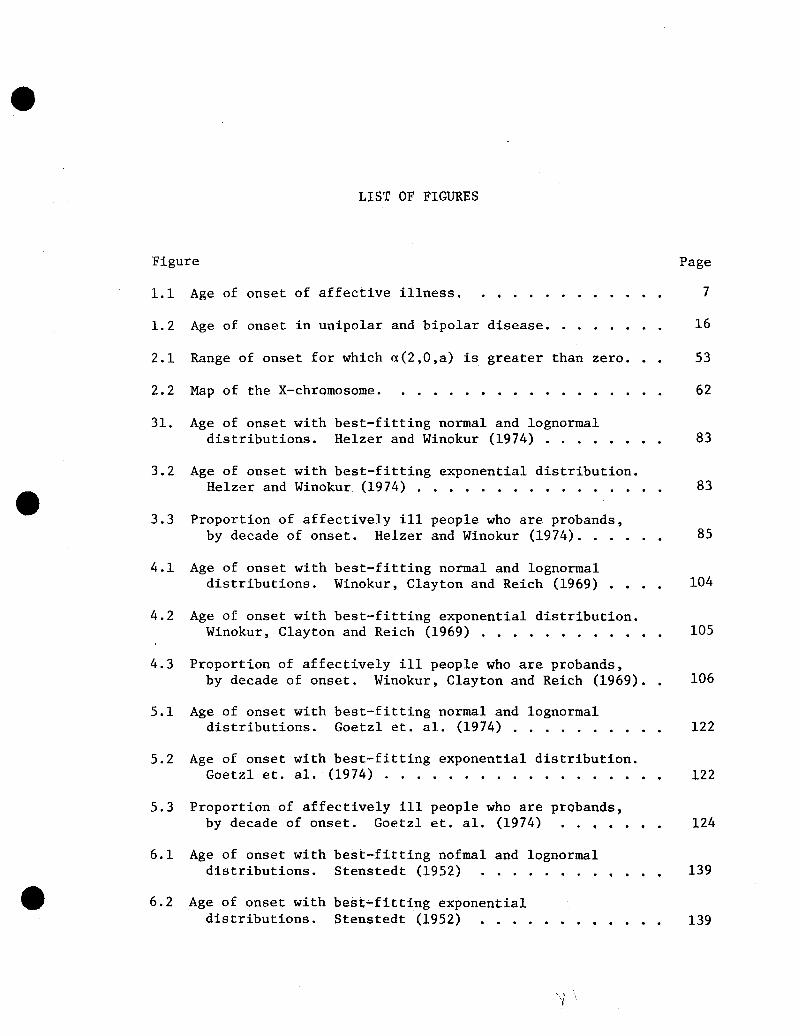
LIST OF FIGURES

Figure

1.1 Age of onset of affective illness. . ....Page

7

1.2 Age of onset in unipolar and bipolar disease.

2.1 Range of onset for which u(2,0,a) is greater than zero.

2.2 Map of the X-chromosome.

16

53

62

31. Age of onset with best-fitting normal and lognormaldistributions. Helzer and Winokur (1974) .... 83

3.2 Age of onset with best-fitting exponential distribution.Helzer and Winokur (1974) . . • • . • . . • . . . . . 83

3.3 Proportion of affectively ill people who are probands,by decade of onset. Helzer and Winokur (1974). . 85

4.1 Age of onset with best-fitting normal and lognormaldistributions. Winokur, Clayton and Reich (1969) 104

4.2 Age of onset with best-fitting exponential distribution.Winokur, Clayton and Reich (1969) . • • . . . . . . . .. 105

4.3 Proportion of affectively ill people who are probands,by decade of onset. Winokur, Clayton and Reich (1969).. 106

5.1 Age of onset with best-fitting normal and lognormaldistributions. Goetz1 et. al. (1974) ....•. 122

5.2 Age of onset with best-fitting exponential distribution.Goetzl et. al.· (1974). .•....••..•.• 122

5.3 Proportion of affectively ill people who are probands,by decade of onset. Goetzl et. a1. (1974) •.••• 124

6.1 Age of onset with best-fitting nofmal and lognormaldistributions. Stenstedt (1952) ...•.•.. 139

6.2 Age of onset with best-fitting exponentialdistributions. Stenstedt (1952) ..•. • • • 41 • • • •

" ") '~

139

Figure

x

Page

6.3 Proportion of affectively ill people who are probands,by decade of onset.' Stenstedt (1952) . . . . . . • 140

7.1 Lava family:relatives .

Pedigree of the proband's first-degree

, ,

152

CHAPTER I

INTRODUCTION AND REVIEW OF THE LITERATURE

The study of the genetics of manic depressive illness has been

hampered by many problems. As with the study of any mental disease,

there are problems with the definition and diagnosis of manic depressive

illness, and with enlisting the cooperation of the families of manic­

depressive probands. These difficulties aggravate complications such

as incomplete penetrance, variable age of onset, and possible genetic

heterogeneity, that make the detection of genes in human populations

difficult. Previous family studies have, for the most part, been

concerned with calculating age corrected risks to various classes of

relatives of manic depressive probands. These risks are then compared

to the segregation ratios expected on various genetic hypotheses. This

method wastes information present in the family structures and does

not have the power to discriminate among genetic hypotheses in the

face of the problems present in the analysis of manic depressive

illness. Genetic hypotheses that have been suggested include a single

X-linked dominant gene, a single autosomal dominant gene, and two-gene

models including one X-linked and one autosomal dominant. Linkage

with X-linked markers has also been tested. While it is quite

generally acknowledged that there is a genetic component in the

etiology of manic depressive illness, no single hypothesis has

achieved widespread acceptance.

2

This thesis will be concerned with the analysis of four sets of

data, all previously reported in the literature, to examine these

hypotheses using Elston's approach (Elston & Stewart 1971, Elston

1973, Elston & Yelverton 1975) to pedigree analysis, which helps

overcome the difficulties present in the analysLs of mental illness.

Previously suggested modes of inherit~ce will be tested, and one

large family with data on manic depressive illness and the X-linked

markers of colorblindness and the Xg blood group will be used for

linkage analysis. Sections 2 and 3 of this chapter will review the

literature on the genetics of manic depressive illness and statistical

methods used to detect genes in human populations, respectively.

Chapter II presents a detailed description of the models to be used

and some extensions to the likelihood method of pedigree analysis.

Chapter III - VI present segregation analyses of the four sets of data,

and Chapter VII presents linkage analysis of a large family.

1.2 The genetic basis of manic depressive psychosis.

Manic depressive psychosis as a disease entity separate from other

forms of mental illness was first described by Kraeplin in the late

1880's (Kraeplin 1907, 1917). Kraeplin's nosological scheme classified

non-organic mental illness into several broad categories: melancholia,

maniacal-depressive conditions, dementia praecox (schizophrenia),

katatonia, and paranoia (Kraeplin 1917). He described manic depressive

psychosis as marked by recurrent attacks of mania and depression

separated by lucid intervals. Recovery from episodes is spontaneous

and there is no progressive mental degeneration as in schizophrenia.

Kraeplin says the prognosis is good in that recovery from individual

3

episodes is almost certain, but poor in that more attacks are likely

in the future (Kraeplin 1907).

Mania is characterized by psychomotor restlessness, flight of

ideas, great impulsiveness, irritability, insomnia, grandiosity, short

attention span, and sometimes delusions or hallucinations. Depression

is characterized by psychomotor retardation, inability to concentrate,

dearth of ideas, despondent view of life, loss of appetite, insomnia,

social withdrawl, and sometimes feelings of sinfulness, worthlessness

or hypochondria. These symptoms, described by Kraeplin, are almost

exactly the same diagnostic criteria used today by Winokur's group

(eg., Winokur, Clayton, and Reich 1969), Mend1ewicz's group

(Mend1ewicz and Fleiss 1974), and others (Abrams and Taylor 1974,

Goetz1 et. al. 1974, Hopkinson and Ley 1969, Gershon et. al. 1973).

Kraeplin's scheme is also quite similar to that of the American

Psychiatric Association (1968) (see Table 1.1), which divides non­

organic psychoses into schizophrenia, major affective disorders,

paranoid states, and other psychoses. The category of major affective

disorders is further subdivided into involutional melancholia (a

form of depression with onset in late middle age); manic depressive

illness, depressive type (unipolar depression); manic depressive

illness, manic type (unipolar mania); manic depressive illness,

circular type (bipolar illness); and other (including "mixed"

disorders with mania and depression almost simultaneously). These

states are all characterized by, among other ~hings, an onset that

is independent of any obvious environmental trigger such as death

of a spouse. A depression occurring after such an event and severe

enough to be called psychotic is a psychotic depressive reaction and

4

Table 1.1 Classification of mental illnesses.

Classification of the AmericanPsychiatric Association (1968)

Kraeplin's classification(taken from Kraeplin (1917)

Melancholia

Delirium, delusions, hysteria

Maniacal-depressive conditions

Melancholia

Imbecility, idiocyCoarse brain lesions, epilepsy

ParanoiaAlcoholic, moral, drug psychoses

Dementia praecox, katatonia

J

I.II.

III.

Mental retardation }Organic brain syndromesPsychoses not attributed to

physical conditions295. Schizophrenia (& subtypes)296. Major affective disorders

.0 Involutional melancholia

.1 Manic depressive illness,manic type

.2 Manic depressive illness,depressive type

.3 Manic depressive illness,circular type

.8 Other major affectivedisorders

297. Paranoid states298. Other psychoses

.0 Psychotic depressivereaction

IV - X. Neuroses, childhooddisorders, etc.

is classified under "other psychoses" (American Psychiatric

Association (1968).

Reports of the frequency of manic depressive illness in the

population vary quite widely. Book (1953) found a lifetime morbid

risk of 0.0007 in Northern Sweden, while Tomasson (1938) found a

lifetime risk of 0.07 in Iceland. The most commonly reported figures,

however, average about 0.005 - 0.01 (Kallman 1954, Rosenthal 1970,

Winokur and Pitts 1965, Stenstedt 1952, Baldwin 1971). Part of the

variation can be explained by differences in diagnostic criteria used

by different investigators, and different methods of study (for example,

5

a study based on hospitalized patients will find lower prevalence than

one based on a population survey that includes milder cases).

Differing genetic, ethnic, and social environments may also contribute

to the differences. It is noteworthy, however, that in nearly all

studies where sex-specific risks were determined women tend to be

affected about twice as often as men, regardless of the overall

population prevalence (Helgason 1964, Kraep1in 1907, Stenstedt 1952,

Kallman 1954, Rosenthal 1970, Baldwin 1971).

Figures on population frequency are generally given in terms of

lifetime morbid risk, which is defined as the probability that a person

in the population under study will develop the disease sometime during

his life if he lives through the risk period (eg., Winokur, Clayton,

and Reich 1969). This implies that the risk period for the disease is

known. For affective disorders the risk period is usually taken as

15 - 60 (Winokur, Clayton, and Reich 1969; Winokur et. al. 1972),

20 - 50 (Stenstedt 1952, Slater 1935), 20 - 60 (Amark 1951, Stenstedt

1959), or 15 - 80 years (Perris 1974). There are two common methods

of estimating the morbid risk in a population where the members are

of variable ages and not all members have passed through the risk

period (Stenstedt (1952) gives a discussion). The simplest is the

Weinberg abridged method. It is assumed that the risk is uniformly

distributed over the entire period of risk. An estimate of the morbid

a

individuals not yet in the risk period, and b = number of individualsm

in the risk period. This is equivalent to giving a weight of 1 to all

6

people who have passed the risk period, a weight of 0.5 to all

people in the risk period, and a weight of 0 to all people not yet

in the risk period. The denominator is then a weighted average of

the number of people in the population.

The other method, devised by Stromgren, is based on the same

principle with a more complicated weighting scheme. The estimate is

aEb.c. ' where a = number of affected individuals, bi = number of

~ ~

1 in the ~th age d 1 ti . k t th iddlpeop e ~ group, an c. = cumu a ve r~s up oem e~

thof the i age group. Usually five- or ten-year age groups are used

and the weights are determined either from previous population surveys

or from the sample.

These methods are both approximations and there are some

objections to their use when the "population" is a specified group

of relatives of probands. For both methods the age of onset distribu-

tion in the population used to calculate weights (or risk period), and

that in the relatives must be similar or else the risk may be

considerably biased (Rosenthal 1970). Also, for the Weinberg method

to be valid the population distribution of age of onset must be

symmetric and there should be no correlation in age of onset between

relatives.

Age of onset distributions (Stenstedt 1952, Slater 1935) for

affective illness have been published for several populations. Within

each study, the distribution tends to be quite similar for men and

women (see Figure 1.1). These distributions, however, are based on

rather broadly defined affective disorders, including bipolar manic

)C..'1

7

Figure 1.1 Age of onset of affective illness •

..-r---------------------~~"'*-_jlf__--_..,oo

.,.oo

L~g

!~N!ioo~~ao-+---lp:::;;;.---r----.,-----.r-----t----t-----..,..---;

. 10.0 20.0 30.0 '0.0 50.0 60.0 10.0 80

)( Males}

y Females Stenstedt (1952)

• Males

() Females} Slater (1935)

8

depression, unipolar depression, and possibly involutional depressions

and thus may reflect the heterogeneity in the data.

The fact that there is a genetic component in the etiology of

manic depressive illness was recognized by workers as early as

Kraeplin, who said that 70% to 80% of the cases had an "hereditary

taint" and recommended that people who "seemed to be predisposed" to

the disease not marry (Kraeplin 1907). The earliest family studies

were done by Vogt (1910) and Hoffman (1921). Vogt examined 108

probands and their first degree relatives and found about 10% of the

parents had manic depressive psychoses. Hoffman examined the relatives

of people with endogenous depressions and found a very high incidence

of manic depressive illness in the children. This study was widely

criticized (for example by Slater (1935) and Stenstedt (1952)) for

use of very broad definitions of manic depressive illness (cycloid

personalities and "quiet humorists" were included as affected), and

for inadequate statistical treatment. Luxenburger (1932) collected

the data of several other investigators, including Hoffman, and found

incidences of manic depressive illness of 30.2% in children of pro­

bands, 12.6% in sibs, 10.6% in parents, 2.6% in nephews, nieces and

cousins, and 4.8% in aunts and uncles.

Some of the earlier investigators constructed quite elaborate

genetic theories. Hoffman hypothesized three independent factors

carrying different weights with a certain total weight necessary for

psychosis and lesser weights causing cycloid personalities. Rudin

(1923) proposed that one autosomal dominant and two autosomal recessive

factors were necessary, and Luxenburger (1932) suggested one dominant

9

and one recessive factor. Slater (1935) criticized the methodology

and conclusions of all earlier studies and collected his own series

from Kraeplin's clinic. He considered as manic depressive illness all

cases with one clear manic and one clear depressive episode, or three

clear depressions where onset was younger than 50. Using StrBmgren

age correction with five-year intervals and a risk period of 20 to

50, he found the morbid risk for manic depressive illness to parents

of probands was 15.4% ± a standard error of 1.6% and to children was

15.8 ± 2.5%. He also criticized the earlier genetic theories, saying

they were premature, improbable, and supported by no real evidence.

He considered manic depressive illness to be transmitted by an

autosomal dominant gene with reduced penetrance. Part of the reduced

penetrance was explained by problems of diagnosis and ascertainment,

and part by the influence of the "genetic milieu." Slater noted the

increased incidence in women but said that X-linkage was unlikely,

and accounted for it by endocrine balance and social factors.

Several other investigators, however, have considered·the possi­

bility of an X-linked factor. Rosanoff, Handy and P1esset (1935)

suggest a rather common autosomal dominant "cyclothymic" factor and

a less common X-linked dominant activating factor. Burch (1964),

drawing parallels between manic depressive illness and autoimmune

diseases, shows the data fit a model of a fairly common X-linked

dominant gene and a less common autosomal dominant. More recently,

Winokur and Tanna (1969), Mendlewicz et. ale (1972), and Taylor and

Abrams (1973) have suggested that a single X-linked dominant may be

responsible for bipolar manic depressive illness in some families.

10

Large twin studies have been done by Rosanoff, Handy and Plesset

(1935), Kallman (1950, 1954), Harvald and Hauge (1965), Kringlen

(1967), Allen et. al. (1974), and others. The special problems of

dealing with twins seem even more troublesome when mental disorders

are considered. In the early literature there is almost certainly an

over-reporting of concordant monozygotic twins (Rosanoff, Handy and

Plesset 1935). The special shared environment of twins may tend to

produce an excess of concordant pairs. Also, there has been some

suggestion that just being a twin may increase the likelihood of

mental disorders; for instance, Munro (1965) found 11 of 153 of his

probands with primary affective illness were one of a set of twins,

while only 3 of 163 controls had a twin. Tienari (1963) found a

similar situation for schizophrenia. However, several large

population surveys found no increased incidence of mental disorders

in twins over the general population (Harvald and Hauge 1965,

Kringlen 1967). In general, the studies have shown higher pairwise

concordance rates for monozygotic than dizygotic twins, and for

bipolar than unipolar disease (see Table 1.2). Rosanoff, Handy and

Plesset (1935) separated their sets by sex and found higher

concordance in female than male pairs, although the numbers were

quite small.

The likelihood that affective illness is not a genetically

homogeneous entity has been recognized for a long time. Slater (1935)

says, "We have little ground for supposing the clinical entity, which

is a matter of conception and convenience, and the underlying genetic

entity correspond." The major division made in order to obtain a

11

Table 1.2 Pairwise concordance rates.

Reference

Monozygotic probandBipolar Unipolar

II % II %

Dizygotic probandBipolar Unipolar

II % II %

Allen et. al. 1974 5 20 10 40 15 0 10 0Harvald & Hauge 1965 15 67 40 5Kring1en 1967 6 33 21 0Kallman 1950 23 96* ? 61* 52 26* ? 7*Luxenburger 1932 4 75 13 0Rosanoff et. al. 1935 ~ 14 71 ~ 27 22

0' 9 67 d'8 25opposite sex 32 9

*age-corrected rates

more homogeneous group of probands is between unipolar and bipolar

illness. Bipolar illness is defined, quite uniformly by various

investigators, as an affective illness with at least one clear-cut

episode of mania and one of depression (Slater 1935; American

Psychiatric Association 1968; Perris 1968a; Winokur, Clayton andG

Reich 1969; Mendlewicz and Fleiss 1972; Goetzl et. al. 1974).

Unipolar mania is usually reported to be quite rare: Perris (1968a)

reports 4.5% of patients exhibiting mania have unipolar mania, and

Bratfos and Haug (1968) find 2%. An exception is Abrams and Taylor

(1974) who find 28%. Unipolar manics, when found, are usually

considered to have bipolar illness.

Unipolar depression is generally diagnosed in one of two ways:

either by at least one clear cut depressive episode with no mania

(Winokur, Clayton and Reich 1969; Winokur 1970, Goetzl et. al. 1974,

~lendlewicz and Fleiss 1974), or by at least three depressions with no

12

mania (Slater 1935; Perris 1968a, 1969). Perris (1968a, 1968b) argues

in favor of using three depressive episodes to define unipolar

illness on the grounds that manic depressive illness is defined as a

recurrent disease and one or two isolated depressions are not suf-

ficient. Also, in about two-thirds of bipolar cases the first episode

is a depression (Kraeplin 1907, Stenstedt 1952, Perris 1968b), so a

person who had had only one depression may well change polarity with

the next episode. Perris (1968b) finds, however, that only 15% of

patients who have had three consecutive depressions and no mania have

a manic episode at some later date. Thus, he says requiring three

depressions provides a reasonable cut-off point for diagnosing

unipolar illness.

However, this criterion eliminates many (mostly young) people who

have had one or two depressions and have not yet passed enough of the

risk period to have had three depressions, thus exaggerating the age

of onset problem. Also, bipolar illness needs only two episodes to

•be defined while unipolar needs three. The average number of

depressions per unipolar patient may be less than three (Stenstedt

1952, Helzer and Winokur 1974; Perris 1968b quotes others' results).

Even Perris (1968b, 1969), using a minimum of three depressions to

define unipolar illness, finds the average number of episodes to be

only 4.2. However, it seems that for purposes of finding morbid

risks to relatives of unipolar probands, the definition makes very

little difference. Perris (1968b), using three depressions, finds

the morbid risk to first degree relatives is about 11%. Winokur et. a1.

(1972) using one depression find a risk of about 14%, and Mendlewicz

13

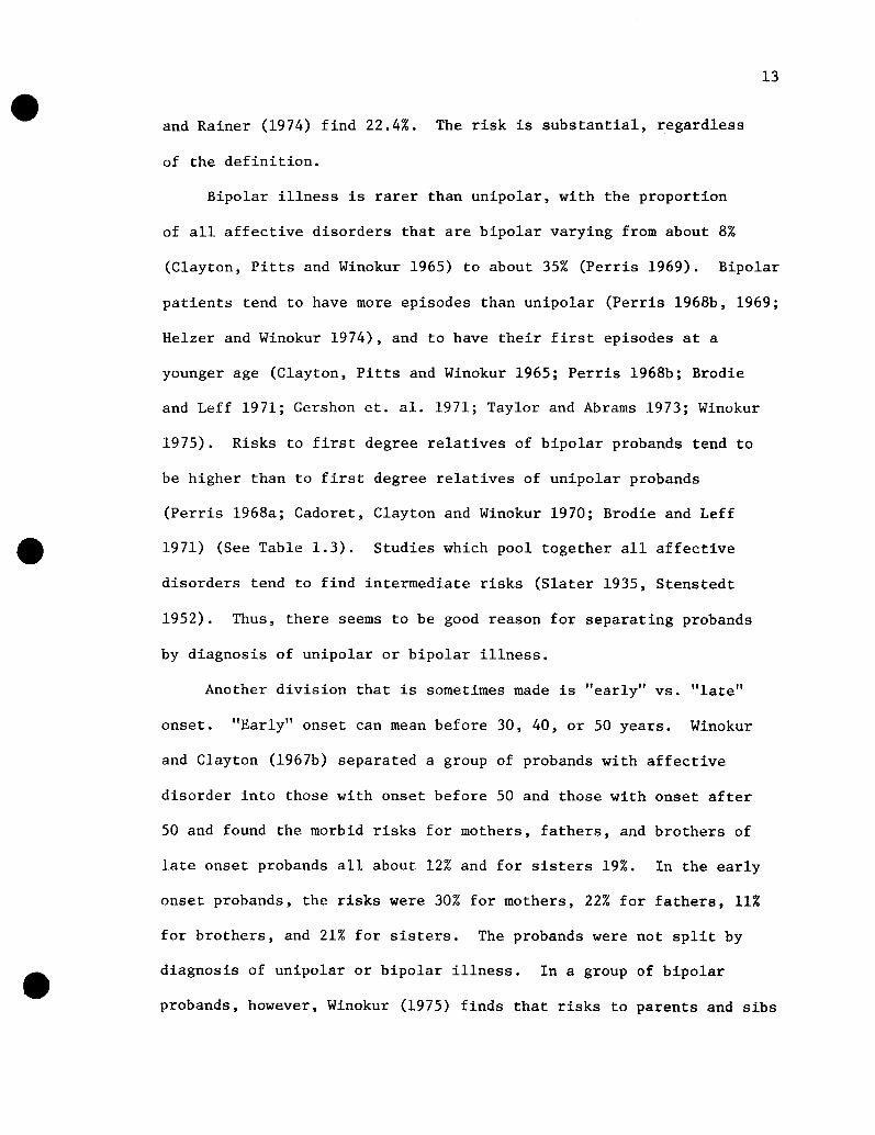
and Rainer (1974) find 22.4%. The risk is substantial, regardless

of the definition.

Bipolar illness is rarer than unipolar, with the proportion

of all affective disorders that are bipolar varying from about 8%

(Clayton, Pitts and Winokur 1965) to about 35% (Perris 1969). Bipolar

patients tend to have more episodes than unipolar (Perris 1968b, 1969;

Helzer and Winokur 1974), and to have their first episodes at a

younger age (Clayton, Pitts and Winokur 1965; Perris 1968b; Brodie

and Leff 1971; Gershon et. al. 1971; Taylor and Abrams 1973; Winokur

1975). Risks to first degree relatives of bipolar probands tend to

be higher than to first degree relatives of unipolar probands

(Perris 1968a; Cadoret, Clayton and Winokur 1970; Brodie and Leff

1971) (See Table 1.3). Studies which pool together all affective

disorders tend to find intermediate risks (Slater 1935, Stenstedt

1952). Thus, there seems to be good reason for separating probands

by diagnosis of unipolar or bipolar illness.

Another division that is sometimes made is "early" vs. "late"

onset. "Early" onset can mean before 30, 40, or 50 years. Winokur

and Clayton (1967b) separated a group of probands with affective

disorder into those with onset before 50 and those with onset after

50 and found the morbid risks for mothers, fathers, and brothers of

late onset probands all about 12% and for sisters 19%. In the early

onset probands, the risks were 30% for mothers, 22% for fathers, 11%

for brothers, and 21% for sisters. The probands were not split by

diagnosis of unipolar or bipolar illness. In a group of bipolar

probands, however, Winokur (1975) finds that risks to parents and sibs

14

+Table 1.3 Morbid risks to relatives (%) .

Reference

Parents

Mo. Fa. All

Sibs

Sis. Bro. All

Children

Dau. Son All

I. Bipolar Probands

57.1** 28.6**76.9** 57.1**

12.0

27.0 22.09.1 10.0

46.0 23.039.0 30.044.0 27.0 35.0

18.2 9.4

10.3

18.812.5

1. 9 11. 2

50.0 23.063.0 0.056.0 13.0 34.0

Mend1ewicz & Rainer 33.7 39.2 59.0(1974) :..:c..::;..__--"-"'-'-' ..:c.:- --"-..;;....;...;'-.-

Winokur et. a1(1972)

Perris (1968a)Winokur, Clayton

& Reich (1969)!t probandt proband

overallGoetz1 et. a1.

proband ~ 24. 2(1974)probandg 18.2

II. Unipolar Probands

Winokur et. a1.(1972)

Cadoret, Winokur,& Clayton (1971)~ probandi5' proband

Perris (1968a)

12.8

16.1 7.114.1 18.2

5.4 4.5

15.3

25.86.6

11.4

8.84.9

6.4

9.7

9.40

6.04

24.1

13.815.8

2.53

5.06

9.0

6.04 10.0

12.7

5.48 6.62

10.27 14.29 12.26 14.29

3.4

10.412.0

15.49.79 4.81 7.35

7.22 3.21 5.25

Slater (1935)*Hoffman (1921)*Banse (1929)*Ro11 & Entres

(1936)*Luxenberger (1942)

III. Endogenous depression, or all affective1y ill probands

Stenstedt (1952)"certain""certain"+"uncertain"

**These risks are based onvery small numbers

*Taken from Rosenthal (1970) + Risks areWeinberg or

age corrected by either theStrtlmgren method.

15

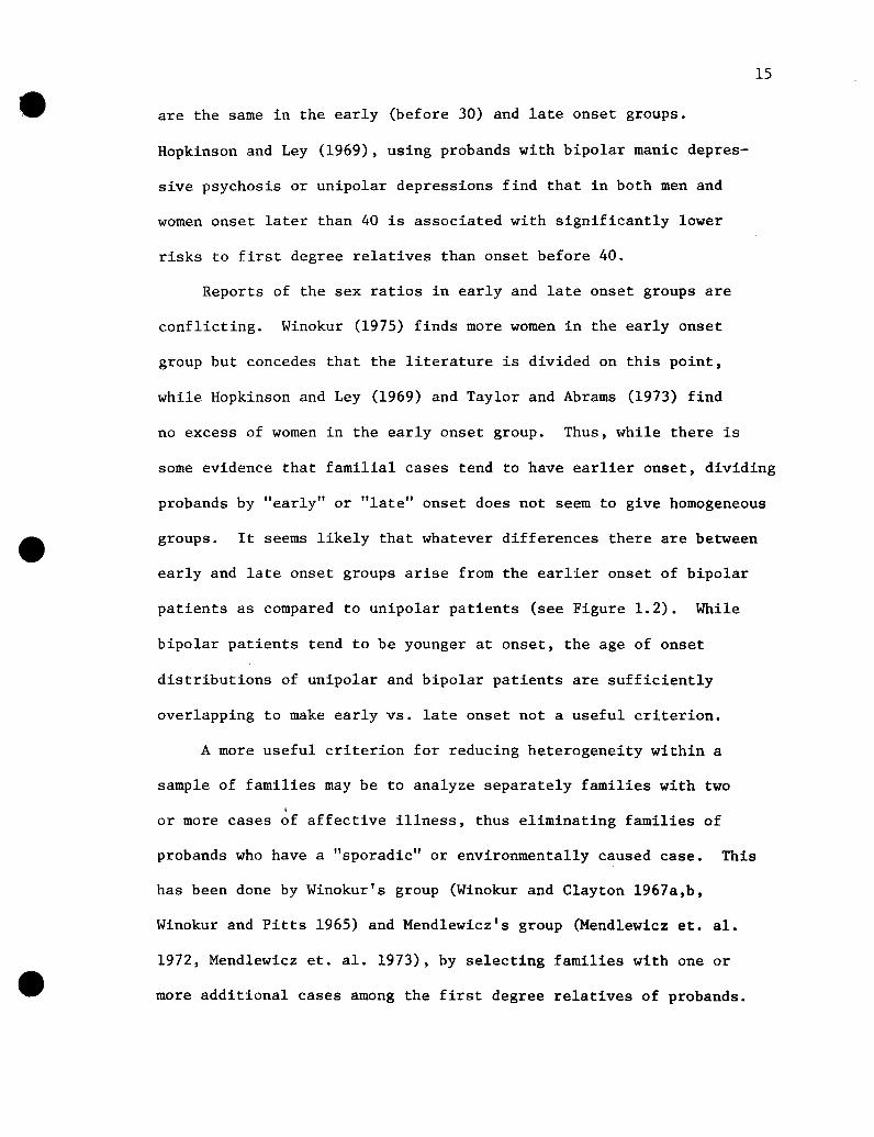
are the same in the early (before 30) and late onset groups.

Hopkinson and Ley (1969), using probands with bipolar manic depres-

sive psychosis or unipolar depressions find that in both men and

women onset later than 40 is associated with significantly lower

risks to first degree relatives than onset before 40.

Reports of the sex ratios in early and late onset groups are

conflicting. Winokur (1975) finds more women in the early onset

group but concedes that the literature is divided on this point,

while Hopkinson and Ley (1969) and Taylor and Abrams (1973) find

no excess of women in the early onset group. Thus, while there is

some evidence that familial cases tend to have earlier onset, dividing

probands by "early" or "late" onset does not seem to give homogeneous

groups. It seems likely that whatever differences there are between

early and late onset groups arise from the earlier onset of bipolar

patients as compared to unipolar patients (see Figure 1.2). While

bipolar patients tend to be younger at onset, the age of onset

distributions of unipolar and bipolar patients are sufficiently

overlapping to make early vs. late onset not a useful criterion.

A more useful criterion for reducing heterogeneity within a

sample of families may be to analyze separately families with twoI

or more cases of affective illness, thus eliminating families of

probands who have a "sporadic" or environmentally caused case. This

has been done by Winokur's group (Winokur and Clayton 1967a,b,

Winokur and Pitts 1965) and Mendlewicz's group (Mendlewicz et. ale

1972, Mendlewicz et. ale 1973), by selecting families with one or

more additional cases among the first degree relatives of probands.

Figure 1.2 Age of onset in unipolar and bipolar disease.

16

x-«i

10.0 20.0 30.0 50.0 60.0 70.0 80

Y Males

)( Females} Bipolar (Winokur, Clayton and Reich 1969)

() Males }• Females

Unipolar (Winokur et ~. 1971)

17

Mendlewicz's group found that the affectively ill people in the

positive family history group had earlier onset with manic and

depressive episodes more nearly equal in frequency than the negative

family history group, and that the positive family history group more

nearly fit the model of transmission of a single dominant gene.

Winokur's group split families on the basis of whether or not the

proband had an affected parent, and found significantly more mania

and more affected sibs in the group of probands with an affected

parent. Ho~ever, none of these studies took into account the manner

in which the sample was selected.

An interesting finding, and possibly a more significant one from

a genetic standpoint, is that it may be possible to form meaningful

groups of probands on the basis of response to drug therapy.

Biochemical theories of mania and depression center around two related

concepts. It has been found that levels of brain neurotransmitters

(norepinephrine and dopamine) are functionally decreased in depression

and increased in mania. Tricyclic compounds (eg., imipramines) and

monoamine oxidase inhibitors (MAOI) are used to treat depressions,

since their effect is to slow the breakdown of the neurotransmitters

(Bunney et. ale 1972, Janowsky 1972). There may also be an upset of

the ionic balance in the nerve endings, and one theory is that the

basic defect may be in the membrane, interfering with the neuronal

uptake process, and associated with ionic balance maintained by the

membrane (Bunney et. ale 1972). Lithium salts are used to treat

both depression and mania (Bunney et. ale 1972; Mendlewicz, Fieve

and Stallon 1973). Studies of drug response in manic depressive

patients and their relatives have been small, but they are suggestive.

18

Angst (1961) found that 66% of 105 people improved when treated

with imipramine for endogenous depression. Of these, there were 9

who had a first or second degree relative who had also been treated

with imipramine. Eight of the pairs had concordant responses; only

one pair was discordant.

Pare et. al. (1962), using imipramines or MAOI on a heterogenous

group of outpatients, found that reactive depressions tend to respond

to MAOI, and endogenous depressions tend to respond to imipramines,

and hypothesized different genetic mechanisms for the two types of

depression. They were also able to find seven proband-first degree

relative pairs treated with the same drug, and all pairs showed

concordant responses. In a later study, Pare and Mack (1971) reported

12 proband-relative pairs (presumably different from the 7 above)

treated with the same drug, and 10 pairs were concordant.

Mendlewicz, Fieve and Stallon (1973), using a more homogeneous

group of 73 bipolar probands in a study of lithium vs. placebo,

found that there was a significant association between positive

response to lithium and the presence of bipolar illness in first

degree relatives.

These studies all ~ggest that affective illness within a family

tends to have the same biochemical (ie., genetic) basis and that

response to drugs may provide a way of discriminating between genetic

and environmental forms of affective illness.

A problem has been raised which is the opposite of trying to

divide affective illnesses in order to get a homogeneous group of

probands: whether there is any reason to subdivide mental illness

into affective disorders, schizophrenia, and so forth. There have

19

been several studies published dealing with the relationship of

manic depressive illness to schizophrenia, involutional psychoses,

and the so-called "mixed" or schizoaffective disorders.

Most studies have found that there is very little, if any,

increased risk of schizophrenia in relatives of manic depressive

probands. Slater (1935), Stenstedt (1942), Kallman (1950, 1954), and

Winokur et. al. (1972) all find morbid risks for schizophrenia

in parents and sibs of manic depressive probands of about 0.5% to

2%. The risk for schizophrenia to the general population is about

0.8% to 1% (Kallman 1954, Rosenthal 1970), so these risks are not

excessively high. The risks to children, however, tend to be

somewhat higher: 1.6% to 3.1% (Slater 1935, Kallman 1954, Rosenthal

1970). This finding has never been satisfactorily explained, but

it seems the simplest explanation is that being raised by a manic

depressive parent can lower the threshold for schizophrenia and

cause a child to show the schizophrenic phenotype when he ordinarily

would not (Rosenthal 1970).

The relationship of manic depressive illness to involutional

melancholia is somewhat hazy. One problem is that unless age periods

are carefully defined involutional melancholia can be confused with

unipolar depression with rather late onset. Stenstedt (1959) using

a possibly heterogeneous group of probands (307 with endogenous

depression including manic depressive and involutional psychoses)

finds risks to sibs of 3.0% for involutional depression and 1.7% for

manic depression; the risks to parents were 1.6% and 0.6% respec­

tively. These figures are not above those for the general

20

population. Rosenthal (1970) finds that the morbid risks for manic

depressive illness are a little higher, on the order of 5%, and

concludes that involutional melancholia is genetically associated

with other affective disorders.

The "mixed" (schizoaffective, schizophreniform, or cycloid)

psychoses are those that can be diagnosed neither as schizophrenia

nor as affective disorders but have some of the characteristics of

each. Whether or not the schizoaffective disorders are a distinct

entity is not agreed upon. Perris (1974) and Mitsuda (1965) consider

schizoaffective disorders as a separate disease. Perris, in a study

of 60 probands, finds morbid risks for schizoaffective disorders in

parents and sibs considerably higher than risks for schizophrenia

or manic depressive illness (20% in parents and 9% in sibs for schizo­

affective disorders; 0% and 1.4% for schizophrenia; 3.1% and 0.68%

for manic depression). Mitsuada (1965), using twin and family

studies, finds no twin pair (out of 16) in which one twin has

schizophrenia and the other a schizoaffective disorder. He also

finds that risks for schizoaffective disorder in families of

schizophrenia or manic depressive probands are small. These studies

support the view that schizoaffective disorders are not generally

related to schizophrenia or affective disorders, but must be

considered as independent.

Clayton, Rodin and Winokur (1968) and Stromgren (1965), on the

other hand, consider the schizoaffective disorders as a symptomological

concept, not a distinct entity. Clayton, Rodin and Winokur, using a

group of 39 probands with schizoaffective disorder, find 11 of their

parents had an affective disorder, and that the risks to first degree

21

relatives for affective disorder is higher than for schizoaffective

disorder or schizophrenia. They conclude that schizoaffective dis-

order is a variant of affective disorder. Stromgren (1965) says

that the schizoaffective psychoses are a heterogeneous group, made

up partly of atypical schizophrenias and partly of atypical affective

disorders.

The schizoaffective disorders are relatively rare, however.

Clayton, Rodin and Winokur (1968) in their series of 426 cases of

primary affective disorder find 39 patients with schizoaffective

disorder. For the most part manic depressive psychoses tend to

"breed true." Gershon et. al. (1971), after an extensive review

of the literature, construct three groups of psychiatric illnesses on

the basis of "common etiologic genetic factors" (see Table 1.4).

Table 1. 4 "Etiologic" groups of psychiatric illnesses.(After Gershon et. al. 1971)

Affective & related

Unipolar depressionPsychotic depressive

reactionBipolar manic depressionInvolutional melan­

choliaAlcoholism (?)Antisocial personality (?)

Schizophrenia & related

Chronic schizophreniaSchizoidParanoidInadequate personality

Mixed

SchizoaffectiveAntisocial (?)Alcoholism (?)Some mental

retardation (?)

It is generally agreed that at least a portion of affective illnesses

are caused to a large degree by genetic factors. The nature of the

genetic factors, however, is still open to question. A major point

22

of disagreement is whether bipolar manic depressive disease is caused

by an X-linked gene, at least in some families. The old observation

that about twice as many women as men are affected is suggestive of

a rare X-linked dominant gene. However, there may be other explana­

tions for the sex ratio. Kallman (1954) says that social factors may

be causing the excess: men have more of an advantage in concealing

the disease, and women have less control over their lives and are

therefore more likely to be hospitalized. Ther~ may also be a slight

excess of completed suicide in men (Kallman 1954, Stenstedt 1952,

Gershon et. al. 1971), although if there is any sex difference it

is not large (Pitts and Winokur 1964, Perris 1969). Slater (1935)

says the sex difference may be due to "different endocrine balance"

in women, and Stenstedt (1952) says manifestation is greater in women

due to "constitution." There has been some suggestion (Brown et. al.

1973) that the overall sex ratio in families with affective illness

is aberrant, with a preponderance of women. This has not been

found in other studies (Winokur and Reich 1970; Cadoret and Winokur

1975 give other references).

A more stringent requirement of the X-linkage hypothesis is

that there be no father to son transmission of the disease. A

number of groups refute the X-linked hypothesis on this basis

(eg., Goetzl et. al. 1974; Perris 1968a, 1969; Von Grieff et. al.

1975). Perris (1968a, 1969) finds morbid risks to sons and daughters

of bipolar men about equal, and that the male to female ratio for

bipolar patients is about one to one. He concludes that bipolar

illness cannot be due to an X-linked gene. Goetzl et. al. (1974)

23

find four instances of male to male transmission in their series of

39 manic probands, as well as an equal number of men and women

affected, and conclude that a locus on the X chromosome "is not itself

a necessary or sufficient condition for the transmission of manic

depressive illness."

Perris (1968a, 1969) finds a preponderance of women among his

unipolar patients, and that risks to daughters of unipolar men are

much higher than risks to sons (although there are a few cases of

father to son transmission). He quotes Angst (1966) as obtaining

results very similar to these, and concludes that unipolar depression,

but not bipolar illness, may be due to an X-linked dominant gene.

Other groups (eg., Taylor and Abrams 1973, Mendlewicz and

Rainer 1974, Reich, Clayton and Winokur 1969) reach exactly opposite

conclusion: that bipolar illness may be due to an X-linked gene but

not unipolar illness. In some studies with bipolar probands there is

no male to male transmission found (Winokur, Clayton and Reich 1969,

Taylor and Abrams 1973, Helzer and Winokur 1974); in others there is

some (Reich, Clayton and Winokur 1969, Mendlewicz and Rainer 1974),

but these people generally conclude that there is heterogeneity of

the disease rather than reject the X-linkage hypothesis.

In further support of the hypothesis, Winokur, Clayton and Reich

(1969) find that the risk bo mothers of female probands is about twice

that to fathers, and the risk to sisters is about twice that to

brothers. For male probands the risk to fathers is 0 and is 63% to

mothers, while the risk to brothers and sisters is about equal (see

Table 1.3). This is apparently the only study (of this group or

24

others) where the risks turned out to support the X-linkage hypothesis

so strongly. Usually, at least a few cases of father to son

transmission are observed, or there is some other abberation in the

sex ratios of observed risks. However, in most studies father to son

transmission of mania is very rare (Dunner and Fieve 1975).

Cadoret, Winokur and Clayton (1971), using unipolar probands from

their Family History Studies series and four other series in the

literature find that sons and brothers of female probands have smaller

morbid risks than daughters and sisters, and that all children of

male probands have about the same risk. They rule out X-linkage for

unipolar depression and hypothesize that there are two subgroups of

depressive illness: one that is sex limited to women and one that is

expressed equally in men and women. There seems to be no simple

explanation for the discrepancy in results of these groups, and the

results of Perris, Goetzl et. al. and others. Gershon et. al. (1976)

conclude, after an extensive review of the literature, that bipolar

illness may be transmitted by an X-linked gene in some families but

that family studies do not suggest that this is the usual mode of

inheritance.

Another hypothesis that has been suggested is that transmission

is polygenic. Slater (1966) used a very simple approach to determine

that if transmission of a disease is polygenic then pairs of affected

relatives should be in the ratio one bilateral (ie., a maternal and

a paternal relative) to two unilateral (ie., two maternal or two

paternal). If transmission is via a single dominant gene then there

should be an excess of unilateral pairs (assuming mating is at random).

25

This model has been applied by Perris (1971) and Slater et. al.

(1971) who find that the polygenic model fits for both unipolar and

bipolar diseases, and by Baker et. al. (1972) who find it fits

unipolar disease. Mendlewicz et. al. (1973) divide their bipolar

patients by those who have at least one first degree relative with

affective illness and those who do not. They find the polygenic model

fits the negative family history group but not the positive family

history group. However, Slater et. al. (1971) point out biases that

can arise in this type of analysis, including an excess of bilateral

pairs caused by assortative mating or the possibility that knowledge

of mental illness on one side of the family increases the likelihood

of its being discovered on the other side.

Another observation of interest is that alcoholism seems to be

more frequent in families with affective illness than would be expected

by chance. Winokur's group, particularly, has looked at this in some

detail (Helzer and Winokur 1974; Winokur, Rimmer and Reich 1971;

Pitts and Winokur 1966; Winokur and Clayton 1967a; Winokur and Reich

1970). They find, in general, that in families with affective

illness alcoholism tends to be increased in men, but not in women.

Winokur and Reich (1970) find that 16% of the fathers of 61 manic

probands were alcoholic, and that 25 probands had alcoholism in the

family, with no difference in incidence in maternal and paternal sides.

Winokur and Clayton (1967a) find the risks for alcoholism in brothers

of affectively ill probands greater than in sisters, and that the risk

for affective illness to sisters of female probands (21.6%) was much

greater than the risk to brothers (7.4%). If it is assumed that

alcoholism is an affective equivalent, risks to brothers and sisters

26

of male and female probands are about equal. However, alcoholism is

not rare enough to assume all alcoholism in the families is affective

disorder. Also the risk for alcoholism in brothers of male and female

probands is about equal, but the risk for affective illness is not.

The increased risk for alcoholism in families with affective

illness apparently does not go the other way, however. Amark (1951),

in a study of alcoholic probands, found increased risk of alcoholism

to fathers and brothers but not to mothers and sisters. The risk to

parents and sibs for manic depressive illness and schizophrenia was

not increased over the general population. It has also been found

(Pitts and Winokur 1966, Rosenthal 1970, Gershon et. al. 1971) that

alcoholism tends to be increased in the families of people with other

mental diseases such as schizophrenia and various neuroses, and thus

the association of alcoholism with mental disease may be rather

nonspecific.

Winokur and Reich (1970), and Morrison (1975), however, suggest

a two gene hypothesis for bipolar manic depression that involves

alcoholism. The risk to first degree relatives of bipolar patients

tends to be less than the 50% expected for a dominant gene. Thus,

the gene either has reduced penetrance or there is more than one

gene involved. Winokur (1970) observes that about 43% of the affec­

tively ill sibs and children of manic probands showed mania, and

points out that this is about what would be expected if there were

another dominant gene that caused mania in the presence of the gene

causing affective illness. In later papers (Winokur and Reich 1970,

Morrison 1975) it is suggested that the second gene may be expressed

27

as alcoholism in the absence of the primary factor. They hypothesize

also that the primary factor causing affective illness is an X-linked

dominant and the second factor is an autosomal dominant. This is

quite an elaborate hypothesis and while it fits much of the data it

has not been rigorously tested.

The hypothesis that bipolar disease is due to an X-linked gene

has recently been tested by linkage analysis (Fieve, Mendlewicz and

Fleiss 1969; Winokur and Tanna 1969; Winokur, Clayton and Reich 1969;

Mendlewicz, Fleiss and Fieve 1972; Mendlewicz and Fleiss 1974).

Winokur and Tanna (1969), using ten two-generational families with

unipolar or bipolar disease and tested for nine blood groups, found

no evidence of linkage between unipolar depression and any of the

markers. However, they found significant evidence of linkage between

bipolar disease and the Xg blood group. The sample was very small

(only two families were informative), and although there was no

information on the mothers' phases they assumed both were in coupling

and counted "recombinants." Winokur's group also has two large

families in which both bipolar illness and colorblindness are present

(Winokur, Clayton and Reich 1969; Reich, Clayton and Winokur 1969).

In these families they find that there are 11 people with the

colorblindness gene and the hypothesized manic depression gene, and

only (possibly) one person with one gene and not the other (one young

man is colorblind but not yet affectively ill). They say the

probability this is due to chance is (.5)11 = .0005, and that this is

strong evidence for linkage.

Mendlewicz and Fleiss (1974) take all the informative families of

Winokur's group, plus 15 of their own, and using lod scores as

28

tabulated by Edwards (1971), find maximum likelihood estimates of

recombination fractions of 0.07 for bipolar-deuteranopia, 0.10 for

bipolar-protanopia, and 0.19 for bipolar-Xg. The maximum lod scores

are 4.47 for linkage with deuteranopia, 3.73 with protanopia, and

2.95 with Xg. If valid, this would be strong evidence for linkage

with both the colorblindness loci and Xg. However, Gershon and Bunney

(1976) have pointed out some of the serious methodological problems

with these studies, and it would be premature to conclude that

linkage between a gene for manic depressive illness and an X-linked

marker has been demonstrated.

1.3 Statistical methods used to detect major genes in human family

data.

There are many problems that arise in trying to detect genes that

cause disease in human populations. Small sample sizes and non-random

sampling are among the more serious statistical problems; genetic

problems include the probable genetic heterogeneity of many diseases,

incomplete penetrance and sporadic cases, and a variable age of onset.

As a result the classical Mendelian segregat~on ratios are virtually

never observed in human families for any traits of interest. Two

major approaches used to detect major genes are segregation analysis

and its variants, and linkage analysis.

Classical segregation analysis calculates the expected segregation

ratios of affected children conditional on parental phenotypes,

assuming a specific one gene model (eg, Morton 1969, Morton et. al.

1971). It can take into account incomplete penetrance, non-random

sampling, and sporadic cases. It must be used on families of parents

29

and their children only, however, and a simulation study (Smith 1971)

shows that classical segregation analysis is not very powerful for

detecting major genes in the face of complications like incomplete

penetrance and a variable age of onset.

Other approaches to the problem of incomplete penetrance have

been made by Trankell (1955, 1956); O'Brien, Li and Taylor (1965);

Defrise-Gussenhoven (1962), Wilson (1974) and others. The basic

model taken by Trankell and by O'Brien et. al. is that of a single

locus with two alleles, resulting in two phenotypes. O'Brien et. al.

consider a recessive gene with incomplete penetrance and calculate

the frequencies of sib-pair phenotypes as a function of the penetrance

parameters and the gene frequency. They derive maximum likelihood

estimates of these parameters. Trankell takes a more general approach.

Each genotype is allowed a different probability of affectation, and

expected proportions of affected children from different mating types

are calculated. These proportions are expressed as a function of the

probability of affectation for each genotype and of the population

gene frequency.

The approach of Defrise-Gussenhoven is to try to discriminate

a two-gene hypothesis from that of a single gene with incomplete

penetrance. The model is of two genes, each with two alleles,

resulting in two phenotypes. Biologically reasonable modes of

interaction of the two genes are considered, and the frequencies of

the phenotypes in children of different mating types are calculated

as a function of the gene frequencies. Similar calculations are made

on the hypothesis of one incompletely penetrant gene, and charts of

30

the distribution of phenotypes as a function of gene frequency are

given to aid in the rejection of unreasonable hypotheses.

Two approaches to analysis of traits with a variable age at onset

have been made by Batschelet (1962, 1963) and Elandt-Johnson (1973).

Batschelet's model is of one locus, two alleles, and two phenotypes.

Assuming Hardy-Weinberg equilibrium and no correlation in age of onset

among relatives, he defines a penetrance function p(x)=Pr(age at

onset~x) and allows for an upper age cutoff beyond which it is assumed

no one acquires the disease. The basic calculation is Pr(k parents

and r sibs [out of s] are affected I ages, genetic hypothesis, and

parental mating type), and is a function of the p(x) for the ages of

everyone in the family. However, Batschelet makes the approximation

of replacing the parents' ages by their average, and the childrens'

ages by their average, which converts the probabilities to products of

binomials. This introduces a bias which gets larger as the sample

size increases. The approximation is not necessary, but only makes

the probabilities easier to write down in a closed form. Batschelet

also considers corrections for ascertainment in the form of single

selection or truncate selection.

Elandt-Johnson (1973) uses a life-table approach to estimate the

probability that a child will be genetically susceptible to a disease

given the parental mating type, when onset of the disease is variable.

Her model assumes that onset is variable but early (so that onset is

complete in the parents), that all susceptible genotypes develop the

disease eventually, and that all parents of a given mating type have

the same segregation pattern. Actuarial-type techniques are used

31

to estimate probabilities of a child developing the disease at age x

and the overall proportion of children susceptible to the disease

from parents of given phenotypes.

Recently, more powerful and general models for segregation

analysis have been devised (MacLean et. al. 1975, Morton and MacLean

1974, Elston and Stewart 1971, Elston 1973, Elston and Yelverton

1975). These methods are based on calculating the likelihood of a

family's phenotypes based on a genetic hypothesis. The method leads

to maximum likelihood estimates of parameters, and hypotheses are

tested by likelihood ratio tests.

An important assumption underlying these models is that there is

no non-genetic correlation in phenotype between parent and offspring.

Violation of this assumption might lead to the detection of a

spurious major gene. Morton's model (Morton & MacLean 1974)

specifically allows for an environmental correlation among sibs.

Elston's model assumes that there is no sibling environmental correla-

tion, but simulation studies (Go et. al. 1977) suggest that the method

is robust against violations of this assumption.

Morton's model is currently programed for the mixed model of a

major gene (with two alleles) plus polygenic and environmental

variation for families of parents and their children. The likelihood

is expressed as

00 3 3 s 3

L(f)=Looj~l k~l ~jku n~l i~lPi,jkPr(~nlgi,u)du

32

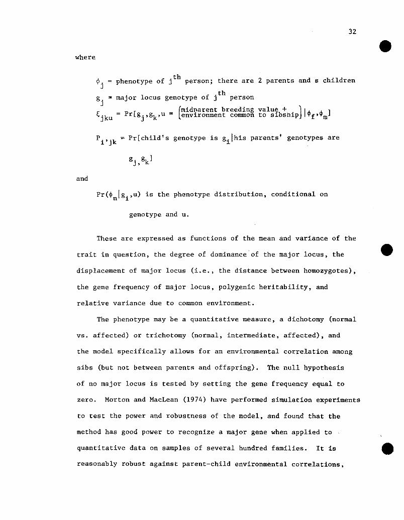
where

phenotype of jth person; there are 2 parents and s children

. 1 f .thmaJor ocus genotype 0 J person

(midParent breeding value + ) I ]

Pr[gj,gk'u = environment common to sibship ~f'~m

= Pr[child's genotype is g.lhis parents' genotypes are1

and

Pr(~ Ig.,u) is the phenotype distribution, conditional onn 1

genotype and u.

These are expressed as functions of the mean and variance of the

trait in question, the degree of dominance'of the major locus, the

displacement of major locus (i.e., the distance between homozygotes),

the gene frequency of major locus, polygenic heritability, and

relative variance due to common environment.

The phenotype may be a quantitative measure, a dichotomy (normal

vs. affected) or trichotomy (normal, intermediate, affected), and

the model specifically allows for an environmental correlation among

sibs (but not between parents and offspring). The null hypothesis

of no major locus is tested by setting the gene frequency equal to

zero. Morton and MacLean (1974) have performed simulation experiments

to test the power and robustness of the model, and found that the

method has good power to recognize a major gene when applied to '

quantitative data on samples of several hundred families. It is

reasonably robust against parent-child environmental correlations,

33

assortative mating, and heterogeneity among families if and only if

the model includes both polygenic variation and sibling environmental

correlation, and tests of heterogeneity are performed.I

Elston's model can, at least in theory, encompass a wide

variety of genetic models, including one- and two-major gene models

(with linkage analysis as a special case), polygenic, and the mixed

model of one major gene plus polygenic background. The likelihood

is formulated for pedigrees of nearly any size and structure, and

can take into account incomplete penetrance, variable age of onset,

and nonrandom sampling.

The likelihood of observing the phenotypes of a family under a

genetic model can be expressed in terms of:

(i)~u' the population frequency of genotype u;

(ii)p ,the probability that a child has genotype u, givenstu

that his parents have genotypes sand t; and

(iii) 8hu (z), the probability (or likelihood) that an individual

has phenotype z, given he has genotype u and sex h (Elston

and Stewart 1971).

The genetic model can be one gene, two linked genes, two unlinked

genes, polygenic, or the mixed model of one major gene with polygenic

background. The type of genetic transmission is expressed in the

transition matrix of probabilities, p . For the one- or two-genestu

models, the p t are discrete probabilities; for the polygenic modelss u

they are expressed in terms of normal densities. The segregation

analysis considered here is concerned with detection of major genes;

therefore models of one or two genes will be of interest. The pstu

34

can then be expressed in terms of transmission probabilities:

'ss'u = Pr(genotype sst transmits allele u). For one autosomal

locus with two alleles, the matrix P = (p ) is 3x3x3, and under- stu

Mendelian inheritance, 'AAA = 1.0, 'AaA = 0.5, and 'aaA = 0.0.

The phenotypic model is expressed in the distributions g (z).u

Phenotype may be a continuous measure, or categorical with two states

(as in a disease) or multiple states (as in some blood groups, for

example). The distributions may be formulated to take into account

such things as reduced penetrance, sporadic cases of a disease, or

variable age of onset. For example, in the simple case of a partially

penetrant or incompletely dominant gene, where zi 1 if the i th

person is affected, and 0 if he is normal, the phenotypic model might

be

1

f

o

l-f

g (0) = 0aa

g (0) = 1aa

The likelihood of a nuclear family, assuming that it is a random

sample from the population and that there is no environmental

correlation in phenotype among family members, is

where zf = father's phenotype, Z = mother's phenotype, z. = children'sm 1

phenotypes (Elston and Stewart 1971). The likelihood calculations are

easily extended (in theory) to complex families of more than two

generations (Lange and Elston 1975), and to include half sibs and

twins (Elston and Yelverton 197&).

35

The correction for ascertainment is necessary when families

are ascertained through one or more probands. The likelihood of a

family is expressed as L(flassertained through one or more probands)=

L(f)L(one or more probandsl~) (Elston 1973).L(one or more probands)

L(one or more probandslf) is called the ascertainment function.

If we assume that probands are ascertained independently from only

one source, then the ascertainment function for the family is the

product of the individuals' ascertainment functions.

The ascertainment function for an individual is a(zi,bi,ai

)=

thPr(i person has proband status b.1 disease status z , and age of

1 i

onset a.)1

where 1·f h .th . b d dt e 1 person 1S a pro an , an

if he is not.

The ascertainment function for the whole family is

a(~,E.,.9:.) = J}a(z. ,b., a.).1. 111.

where i indexes all individuals in the family. If we let TI(z.,a.,) =1. 1

Pr(a person with phenotype z. and age of onset a. is a proband) then1. 1

(Elston and Yelverton 1975). Various models for TI(zi,ai

) have been

proposed. The simplest is to assume that the probability that an

affected person is a proband is the same for all affected people:

TI(l,a.) = TI, and TI(O,a.) = O.1. 1.

36

The denominator of the conditional likelihood is referred to as

the sampling correction. Define B = Pr(no probands in family). Then

the sampling correction Pr(~ 1 probands in family) = I-B. B is condi-

tional on the size, structure, and ages at examination observed in the

family but not on the phenotypes (disease status, age of onset) of

the family members. It is equal to the multiple intrega1 over ages

of onset and multiple ?ummation over disease statuses of the numerator,

with all proband statuses, b. set equal to 0 (Elston 1973). The1

calculation of B is somewhat simplified by the fact that in the

expression for L(f) there is just one factor for each person that

depends on his phenotype. Therefore, the order in which operations

are carried out may be rearranged and the numerator (for a two-genera-

tiona1 family) is

, , nE~ a(zf,b f ,af )gl (zf,af,af)L~ a(z ,b ,a )gZt(z a ,a ).TI1Epssstt m m m m, m m 1= u stu

a ( z . , b . ,a. ) gh u (z . ,a ~ , a . ) ,111.111

1 . __....-_

where h = I if a person is male and h = 2 if female.

The integration and summation can be performed separately for each

person, so that B depends on functions

r;h u =i

fa. Z ,

1 E a (z ., 0 , a . ) gl ( Z. ,a . , a . ) d_('0 Zj =0 1 1 Ii lJ 1 1 1 a i

(Elston and Yelverton 1975). r;h may be interpreted as the prob­.u1

ability of not being a proband by age a~, conditional of sex hi and

genotype u. B can be calculated using the same algorithm as L(f),,

with r;h ~eplacing gh (z.,a.,a.). It depends on the partieular.u .u 1 1 11 1

forms of the ascertainment and phenotypic models.

37

If there are N families (assumed independent) in the sample

then the likelihood of the sample is L = WL(fi)L(ascertainmentl~l.i=l l-8

i

Maximum likelihood estimates of the parameters of the model are

obtained via a search algorithm (Kaplan and Elston 1973). Hypotheses

are tested by likelihood ratio tests. An hypothesis corresponds to

placing restrictions on one or more parameters, and the likelihood

is maximized both in the unrestricted case and under the hypothesis.

If L denotes the unrestricted maximum likelihood and L k denotesr r-

the maximum likelihood with k independent restrictions on the r"-

parameters, then 2 (lnL - I.nL k' is asymptotically distributed as ar r-

X2 with k degrees of freedom under the null hypothesis (see, ego

Kendall and Stuart 1973).

When the principal question of interest is whether or not there

is a major gene, hypotheses about the transmission probabilities

T I are tested. The null hypothesis that there is a major geness u

corresponds to fixing the T'S at their Mendelian values. For an

autosomal locus the hypothesis is Ho

: TAAA

= 1.0, TAaA = 0.5,

2TaaA

= 0.0, and the X has 3 degrees of freedom. The "environmental"

hypothesis of no vertical transmission is Ho

: TAAA

= TAaA = TaaA

,

2and the X has 2 deg~ees of freedom.

Linkage analysis attempts to find an association of phenotypes

within families that is not present in the general population. Two

genetic loci are said to be syntenic if they are on the same

chromosome, and are linked if they are on the same chromosome close

enough together so that there is an association of phenotypes

within families. If it is possible to demonstrate linkage between

38

an hypothesized locus for a disease and a well-known marker locus

(such as a blood type), then this is convincing evidence that there

is a major gene that causes the disease, since it is difficult to

construct situations where an environmentally-caused disease could

mimic linkage with a marker locus.

The problem of detecting linkage would be simple were it not

for the process of recombination, or crossing-over. At a certain

stage in the formation of gametes, homologous chromosomes are paired

and genetic material can be exchanged within a pair. This means

that it is not particular alleles that are linked, but only the loci:

in an equilibrium population there is no association of traits due

to linkage. The recombination fraction, A, is defined as the

proportion of offspring that have genotypes different from the

parental genotypes. For example, in a mating DdMrn x ddmm the off­

spring are of four types: DdMrn, ddrnrn (the parental types), ddMrn, and

Ddrnrn (the recombinant types). With no linkage, the expected

"recombination" fraction is .5, since all types are equally likely.

Values of the recombination fraction less than .5 indicate some

association of loci. Only certain mating types are capable of giving

information on linkage; one parent must be heterozygous at both loci,

and neither parent can be homozygous for a dominant at either locus.

The most informative mating is a double backcross DdMrn x ddmm. X­

linkage is the easiest to deal with, since if it, is known that both

traits are X-linked then they are on the same chromosome, and all

informative matings are essentially double back-cross (ie.,

DdMrn S x dm t- ). Problems in detecting linkages in human data include

39

fairly small family sizes, inability to control matings, and the

small prior probability that two random loci are linked.

Early methods of detecting linkage in human data included the

Fisher-Finney u-scores, Penrose's sib-pair methods, and the

probability ratio test suggested by Haldane and Smith. Fisher

(1934, 1935) suggested modifications of Bernstein's scores that

resulted in a maximum-likelihood scoring procedure, appropriate for

detecting linkage from two-generational data. The method was further

developed by Finney (1940 - 1943). Fisher (1935) showed that the

method is fully efficient in the limit for loose linkage, but the

efficiency approaches zero as the recombination fraction approaches

zero.

Haldane and Smith (1947) described a probability ratio test to

detect linkage from families of any size, without the assumption of

normality required by maximum likelihood scoring. Smith (1953b) shows

that the method of u-scores and the sib-pair method are also forms of

the probability ratio test.

Morton (1955) was the first to suggest using the sequential

probability ratio test. This test has the advantage of having the

smallest expected sample size on the null or alternative hypothesis,

and Morton (1955) shows that the mean expected sample size (averaged

over a "reasonable" range of alternate hypothesis recombination

fractions) of the sequential test is about one-third that required

by a u-score test with the same error probabilities.

The assumptions required for the test are: (1) parental genotypes

are known with certainty except for phase, (2) segregation ratios

40

are not disturbed by incomplete penetrance or differential

viability, (3) the method of ascertainment and selection of families

in properly allowed for (Morton 1955). Alternatives to the null

hypothesis of no linkage (A = .5) include the negation of any of

these assumptions, nonrandom segregation of nonhomologous chromosomes,

or linkage. The test procedure is based on lod scores, defined as

Zi = 10glO (~~ ~~~-I ~5n, where Pr (f i IA) is the probability of observing

the i th family if the recombination fraction is A. Values of the lod

scores have been extensively tabulated by Morton (1955, 1957,

Steinberg and Morton 1956, Smith 1968, 1969, Maynard-Smith et. al.

1961, Edwards 1971), and others. The total score for the sample is

2 Lzi

. Morton suggests using a small type I error probability,

a = 0.001, in order to exclude as many false linkages as possible.

Since the a priori probability that two random autosomal loci are

linked is on the order of 1/22 = 0.045, about 4 in every 100 pairs

of loci are on the same chromosome. If the usual significance level

of 0.05 is used, about 5 of every 100 pairs will be detected as

"linked" when they are not, and thus such a test would detect more

false than true linkages (Smith 1953b). Using a = 0.001 helps correct

this. For this a, and power of the test of 0.90, the stopping rule

is to accept linkage (at the nominal value Qf AI) if Z~3 and reject

linkage (ie., accept~= .5) if 2<-2.

Morton's original paper derived in detail the lod scores for

autosomal loci with two alleles. Ascertainment corrections were

derived for selection in either or both factors. Later papers

extended the method to multiple alleles at the marker locus

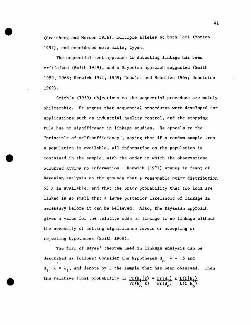
41

(Steinberg and Morton 1956), multiple alleles at both loci (Morton

1957), and considered more mating types.

The sequential test approach to detecting linkage has been

criticized (Smith 1959), and a Bayesian approach suggested (Smith

1959, 1968; Renwick 1971, 1969; Renwick and Schultze 1964; Denniston

1969).

Smith's (1959) objections to the sequential procedure are mainly

philosophic. He argues that sequential procedures were developed for

applications such as industrial quality control, and the stopping

rule has no significance in linkage studies. He appeals to the

"principle of self-sufficiency", saying that if a random sample from

a population is available, all information on the population is

contained in the sample, with the order in which the observations

occurred giving no information. Renwick (1971) argues in favor of

Bayesian analysis on the grounds that a reasonable prior distribution

of A is available, and that the prior probability that two loci are

linked is so small that a large posterior likelihood of linkage is

necessary before it can be believed. Also, the Bayesian approach

gives a value for the relative odds of linkage to no linkage without

the necessity of setting significance levels or accepting or

rejecting hypotheses (Smith 1968).

The form of Bayes' theorem used in linkage analysis can be

described as follows: Consider the hypotheses H : A = .5 andI a

H1

: A = A1

, and denote by E the sample that has been observed. Then

the relative final probability is Pr(Hl~) = Pr(Hll x L(~U!11Pr(H~) Pr(H) L(~ H )000

42

(Smith 1968). The prior distribution of the recombination fraction

is usually taken as uniform on the interval (0,0.5), with

Pr (A = 0.5) = 0.95.

When the alternate hypothesis is not the simple one A = some

specified value A1

, but H1

: the two loci are linked, the relative

final probabilities can be calculated as

kJ;pr(A) L(IIA)dA.

Pr(H ) L(I IDo 0

The numerator represents the average value of the posterior proba-

bility on the alternate hypothesis. This can be approximated by

assuming A takes on only discrete valueg such as 0.00,0.01, ••• ,0.49

and replacing integration by summation (Smith 1959, 1963; Denniston

1969). The Bayesian method has been extended to more than two loci

(Renwick 1971, Renwick and Bolling 1971), but human applications are

scarce and prior distributions of map intervals become difficult.

Regardless of whether a Bayesian or sequential approach is used,

the basis of the analysis lies in the 10d scores or their antilogs.

The basic calculations and the ascertainment corrections are the

same in either case.

Some of the problems involved in linkage analysis are minimzed

when X-linked loci are involved. Recombination is then observed

only in women, so every informative mating is essentially a double

backcross with respect to sons. Phase in a doubly hetero~gous

woman can be determined from the phenotype of the father. If both

loci are known to be X-linked, they are obviously syntenic and the

only question is whether linkage is close enough to be demonstrated.

43

Lod scores and ascertainment corrections have been tabulated

for two- and three-generational families (Smith 1968, 1969; Edwards

1971). Although usually only sons are informative for linkage,

daughters can be used if the father has recessive (or codominant)

alleles at both loci (Smith 1968). Ascertainment of families is

usually assumed to be through sons with a recessive disease, and a

"family" consists of sons (including daughters if they are informa-

tive), mother, and the mother's father. Fraser (1968) shows that

ascertainment corrections are sometimes needed even when three

generations are used. Situations where this is necessary include

truncate selection* at the disease locus and any selection at the

marker locus, and cases where the _mother's mother is used to determine

the phase or genotype of the mother. Fraser shows, however, that no

bias arises when there is single ascertainment at the disease locus

and truncate selection at the marker locus.

In the linkage studies so far performed on manic depressive

illness data (Fieve, Mendlewicz and Fleiss 1969; Mendlewicz, Fleiss

and Fleiss 1972; Mendlewicz and Fleiss 1974) tables of lod scores

as tabulated by Edwards (1971) have been used. These tables were

constructed under the assumption that selection at the marker locus

is independent of disease locus phenotypes. Gershon and Matthysse

(1977) point out that this may not be the case for some of the

affective illness data since the probands are usually colorblind,

manic depressive males. They derive the proper ascertainment cor-

rections when selection of families is through "doubly ill" probands.

*If A = Pr(an affected person is a proband, then truncateselection corresponds to A = 1 and single selection to A~.

44

Comparisons of results obtained with two generation and three

generation families were made by Fraser and Mayo (1968). They noted

discrepancies in estimates of A between Xg and G6PD: using two

generations significant evidence of linkage was found (A = 0.26), but

no evidence of linkage was found when data from three generations were

used. Using simulation studies and large samples (1000 two-son

families) they found that the three generational data had larger

maximum lod scores and that values of Al up to about 0.3 could be

detected. If there was no linkage, this could be detected when

Al = 0.33. In two generational data, linkage could reliably be

detected only up to A = 0.10-0.20, and true H were accepted onlyo

against Al = 0.17 or tighter. They conclude that three generational

data carries far more information than two generations, and "linkages"

detected from two generational data with A as large as 0.25 may not be

linkages at all, even in large samples.

Morton (1955) briefly considers incomplete penetrance or natural

selection in the disease trait. It is assumed that the marker is

fully penetrant, viable, and subject to complete or truncate se1ec-

tion. Then, if the disease is fully penetrant but subvital, linkage

analysis can still be done and the Type I and Type II error prob-

abilities are unchanged. If the disease is not fully penetrant, the

method is still valid but the power will be low if the penetrance is

low.

Ott (1974), using the method of Elston and Stewart (1971) to ca1-

culate the likelihood, takes account of reduced penetrance in the

matrix of probabilities Pr(phenotypelgenotype). The penetrance

parameters can be estimated along with any other unknown parameters

in the likelihood.

45

CHAPTER II

METHODS AND MODELS FOR AFFECTIVE ILLNESS DATA

This Chapter will outline models to be used on the manic

depressive illness data, and present some extensions of Elston's

pedigree likelihood method.

The likelihood of observing a family's phenotypes conditional

on the family being 'ascertained through one or more probands is

L(flmethod of ascertainment) = L(f)L(ascertainmentLtLL(ascertainment)

(Elston, 1973). L(f) is the likelihood assuming the family is a

random one from the population, and is derived under fairly general

conditions by Elston and Stewart (1971). L(ascertainmentlf), the

ascertainment function, can be expressed as the product, over all

individuals in the pedigree, of the individuals' ascertainment

functions, if it can be assumed that probands are ascertained inde-

pendently. The denominator, L(ascertainment) is the same as

L(one or more probands in the family) = l-L(no probands in the

family).

2.1 Specific models for affective illness data.

2.1.1 The phenotypic model

The variables observed include z, the disease status; a, the age

of onset of affective illness; and a', the age at examination.

47

We will assign phenotypes in two ways:

(i) i th person has bipolar manic depressive diseasei th person has unipolar depressioni th person is normal or alcoholic

(ii) Z. = ti2 if i th person has bipolar disease1 1 if i th person has unipolar depression

o if i th person is normalor alcoholism

The age of examination is observed or estimated for all individuals

on whom z. is observed; age of onset is observed for a subsample of1

those with depression and/or mania, but there are no data available

on age of onset of alcoholism. It is assumed that only individuals

with phenotype z = 2 can possibly be probands.

The phenotypic model to be considered is a trichotomy with age

of onset, model I (Yelverton, Namboodiri, and Elston 1975). For

this model the,

gh (zi,a. ,a.).u 1 11

= pr(ith

person has phenotype zilgenotype u and sex hJwith age of onset a.

1

are as follows:

,gh (2 ,a. , a .) = Y2f h ' (a.)

.u 1 1 .u 11 1,

gh (2,a.,?) = YZ' Fh

(a~).u 1 .u 11 1

,~ (l,a.,a.) = ylfh (a.)-hiU 1 1 iU 1

,= ylFh (a.)

iU 1

g' ,hiu(~,ai'-) = 1-(Yl+Y2)Fh.u(ai)

1

where y. = Pr(a person will develop disease form i if he lives long1

enough); fh.u(a) is the density of age of onset, dependent on sex and1

48

a'genotype; Eh (a') = f f h (a) da.u _00 u

i i

The usual form of the model assumes that there is some trans-

formation of age of onset that makes the distribution approximately

normal. This is not a necessary restriction, however, and sampling

corrections will be derived below for the case where f is an

exponential distribution.

In this model it is assumed that the parameters of the age of

onset distribution may depend on sex and/or genotype, while the

susceptibilities (y,) depend only on the form of the diseaseJ.

(unipolar or bipolar).

2.1.2 The ascertainment function

In the case of mental illness data, it may be that the prob-

ability that an affected person becomes a proband depends on his

age of onset. There is evidence for this in schizophrenia (Spence

et. ale 1976). One might expect that the probability of becoming a

proband would decrease with age of onset. An ascertainment model

that allows this is an age dependent exponential function (Elston

and Yelverton (1975):

r.(Ko+Kl a+K2a2

)~(z,a) = mJ.n e ,1 ,

o ,if z = 2.

if z 0,1

2 2where either K2=0, or K2<0 and Kl~4KOK2' If K2<0 and Kl~4K2KO then

2Ko

+Kl

a+K2

ae ~l always, and ~(z,a) can increase to a maximum then

decrease again. If K2=0 then ~(z,a) either increases'to a maximum

of 1 and then remains constant, or decreases with age from a maximum

49

of 1. Elston et. al. (1976) found a quadratic function was necessary

for schizophrenia; a linear or constant function may be adequate for

affective illness.

2.1.3 The sampling correction: l-Pr(O probands in the family).

B = Pr(O probands in the family) can be expressed in terms of

functions ~hu (see section 1.3), which depend on the sex, genotype,

and age at examination for each person, as well as the phenotypic

and ascertainment models. For g and ~ as above,

~hu

ghu (2,a' ,a) da

= 1 - (yl +y2)Fhu (a') + ylFhu(a') + yZ Fhu(a')

= 1

The ~hu for the case were fhu(a) is a normal distribution have

been worked out by Yelverton et. a1. (1975). It has been suggested

(Crowe and Smouse 1976) that age of onset in affective illness may

fit an exponential distribution; therefore 'hu for this distribution

will be derived below.

In this case we have f(a) =(ee-e(a~L) ,a~L. The parametersto ,a~L

are e, a "rate" of onset and L, the lowest age of onset. In theory,

both e and L could be sex and genotype dependent. For simplicity,

we will let 6hu depend on sex and/or genotype, but assume there is

if a~L

50

There are two major subcases: K2<0 and K2=0.

1.

Here

always, so

l;hu

[2.1]

The exponent equals

Therefore,

[2.1]

1 - Y26hu/_~ exp\ 2

K +6h Lo u

x

[K -6 J-12iC (L+ 1 hU)

2 2K2 [2.2]

Where

1 2

Jx ! -202 (t-~)

;-;;::::z edt.-<Xl 21T0

That is,

51

!;hu= {[2.2l for a'~L

1 for a'<L

The !;hu may be readily derived for cases which do not fit the

2restrictions K2<O and Kl~4KoK20 These restrictions imply that the

probability of being a proband increases with age of onset up to a

certain point then decreases. This model is reasonable for many

cases in practice and in particular may be appropriate for mental

illness data.

Thus the cases Kl>O and Kl<O must be considered separately.

If Kl>O, then

a(z,O,a)Ko+Kla

if 2 and Ko/Kl= e z = a<

if z = 2 and a~ Ko/Kl

if z = 0 or 1

There are several subcases depending on the relationships among

a' ,L, and -Ko/Klo If a'~L then fhu(a') = Fhu(a') = 0, and

ghu(2,a' ,a) = ghu(l,a' ,a) = 0 and ghu(O,a' ,-) = 1, so that !;hu = 1.

52

In the cases where a'>L,

1;; =hu

[2.3]

Where the limits of the integral (q and r) differ according to the

relationships among a' ,L, and -Ko/Kl

: the integration is performed

over values of a for which a(2,O,a) is not zero.

[2.3] reduces to

-6 (a-L)hue

[2.4]

In the present case, a(2,O,a»O if a<-K /K and the major subcaseso 1

are L<-Ko/K1 and L~-Ko/Kl (see Figure 2.1 (A))

If L<a' < - Ko/Kl then q = Land r = a', so

((K -8 )a' (K -8 )L1

1 hu 1 hu Je -e

53

Figure 2.1 Range of age of onset for which a(2,O,a) isgreater than zero.

KA.

0a<- _.K •1

t I I a or _00 , ( a

0 L-Ko -Ko L

K1 Xl

B.Koa>- K1

_00 J I I ~a or aK L 0 L K

0 0--K1K1

54

KIf - KO

~L<a, then a(2,0,a) = ° for all a>L, so ~2 = 0.1

Summarizing and simplifying these results,

~u = 1 ,if a'~L

-Ko- S:L<a'Kl -

1-Y2[

_e(K1-ShU)L ])

-6 (a'-L)hu

+ Y2e

If Kl

<0, then

K +6h L [6 0 .uhue 1

Kl -6hu

Ko

, if L<- K s:a' .1

-Kif L<a' < -.2.

Kl

a(z,O,a) =

°1 z = °or 1

This case is similar to the previous one, and ~hu is of the same form.

Let ~l' ~2' q, and r be defined as in [2.4]. The major subclasses

here are L>-K /Kl

and L< -K /K (See Figure 2.1).- 0 0 1

[K ] K +6h L

-6 - --.Q - L -6 (a' -L) 6 e 0 ul: = hu Kl + hu + -:...h_u _"'2 -e e K -6 x

1 hu

If -Ko/Kl~L<a', then q = Land r = a' so

55

K +Sh L-S (a'-L) Shue 0 u

e hu -1 + --::.::.~---Kl-Shu

Simplifying and summarizing these results,

~u: 1, a'.$L

1 -[

-Shu (~+L)Y l-e 1-

Z

YZShu e(Ko+6hUL+(Kl-ShU)a')

K1-Shu

KL<- ~ <a'

Kl

KL<a'~- .-Q., K

1

56

In each case of the age dependent threshold model there is one

term that depends on age and one that depends only on sex and

genotype.

2.1.4 Genetic models

The genetic models to be used are those suggested by previous

studies on the genetics of manic depressive illness. Among the

simple models suggested are a single X-linked dominant gene, a single

autosomal dominant gene, and two gene models with one autDsomal and

one X-linked dominant.

A model of a simple autosomal dominant has been proposed, but

this cannot explain the excess of affected women, or the deficiency

of affected sons of affected men. It is possible that environmental

or social factors, or genetic factors unrelated to the primary

affective illness gene are responsible for these observations.

Allowing sex and genotype dependencies in the age of onset dis-

tribution parameters may explain sex differences without necessarily

requiring an X-linked gene. A model of a single autosomal gene is

the simplest possible. The matrix of transition probabilities,

P t ' has dimensions 3x3x3 and is independent of sex.s u

The other single gene model that has been proposed is that of

an X-linked dominant. Support for the model comes from the observa-

tions that prevalence of affective disorder in women is about twice

that in men, and that affected men have a deficiency of affected sons

and fathers. There are, however, exceptions to the requirement for

the X-linked model that there be no father to son transmission of

the disease. In nearly every study there are at least a few

57

father-son pairs where both are affectively ill. If there is an

X-linked gene for manic depressive illness, then these pairs might

be explained as incomplete penetrance (ie., the mother has the

defective gene but does not show the disease), or as sporadic cases

(ie., either the father or the son is genotypically normal, but has

the disease anyway). Pedigree analysis should be able to account

for these situations.

For an X-linked model the matrix of transition probabilities

must be modified. There are now only two possible genotypes for

men, so the dimensions are 2x3x2 for sons (if "s" is the father's

genotype) and 2x3x3 for daughters. In the likelihood of the family

(L(f» and the sampling correction (S) the summations over p ts u

depend on the sex of the child.

Several two gene models for the inheritance of manic depressive

illness have been proposed (Winokur 1970, Rosanoff et. al. 1935).

These models both involve one autosomal dominant and one X-linked

dominant gene. In Winokur's model, primary affective illness is

caused by an X-linked gene, with a second autosomal dominant gene

necessary for mania. Alcholism may be one way in which the secondary

(autosomal) factor is expressed in the absence of the primary factor.

This model therefore has three or four phenotypes, depending on

whether alcoholics are counted as a separate class.

Rosanoff et. al. (1935) proposed a model wherein both a

cyclothymic autosomal dominant gene and an activating X-linked gene

are necessary for mania and/or depression. Only two phenotypes,

affectively ill and normal, are considered in this model.

58

Another two gene model may be used in an attempt to detect

heterogeneity. Here either an X-linked or an autosomal gene

segregating within a family may cause manic depressive illness while

in the population both genes are present. Allowing both genes in the

model may split the sample into two parts: one in which an autosomal

gene is segregating and one in which an X-linked gene is segregating.

There are, of course, many other ways in which genes at two

loci may interact. For two autosomal loci, there are 50 distinct

ways in which the 9 genotypes can be split into two phenotypes

(Hartl and Maruyama 1968). If one of the loci is X-linked there

will be more since the sexes must be considered separately. The

models outlined here seem most reasonable, based on examination of

the data and previously suggested genetic mechanisms. See Table 2.1

for a summary of the genotype-phenotype correspondences in the

models considered.

For two gene models the genetic transition matrices may be

generated from the corresponding single gene matrices as follows.

Let P and P be the genetic transition matrices appropriate for the-x -a

X-linked and autosomal loci, respectively. Then the genetic

transition matrix for the loci together is

P = P lIP P-a -x

P 4P P'-a -x

if P is 3x2x3 or 3x2x2-x

if P is 2x3x3 or 2x3x2-x

(Elston and Stewart 1971). The Kronecker product of two three-

dimensional matrices is given by Elston and Stewart (1971). ! may

Table 2.1 Genetic models for affective illness.

Females Males

59

One gene models: AA Aa aa Aa Aa aa

Autosomal GItlBJ GIiIiJBB Bb bb B. b.

X-linked CiIiJLI CLGJ

M M N

M M N

D D N

I I N

I I N

N N N

I I I

I I I

I I N

Two Gene models:

(1) Winokur 1970

(2) Double dominant

(Rosanoff et.al.1935)

(3) Heterogenity

AA

Aa

aa

AA

Aa

aa

AA

Aa

aa

BB

BB

BB

Bb

Bb

Bb

bb

bb

bb

B. b.

:~aa~

B. b.

AA~W1j

B. b.

:~aa tttti

I = Affectively ill, M= mania, D= depression, N= normal.

60

also be expressed in terms of .'s. Since an autosomal and an X-

linked gene must be unlinked, • = • T for femalesss'xx'uy ss'u xx'y

and. = • • for males.ss'x.uy ss'u x.y

A subset of the data may be used to test for linkage between a

gene for manic depressive illness and an X-linked marker. It has

been suggested that there is such a linkage with the Xg blood group

(Fieve et. al. 1973, Winokur and Tanna 1969), colorblindness

(Winokur, Clayton and Reich 1969), or both (Mend1ewicz and Fleiss

1974). A map of the X-chromosome (Berg and Bern 1968, Levitan and

Montagu 1971) indicates that it is unlikely that linkage between a

locus for manic depressive illness and both Xg and co10rb1indness

would be detected (see Figure 2.2). The methodological problems in

the studies suggesting these linkages may be sufficient to cause the

detection of nonexistant linkages. An analysis including a variable

age of onset for manic depressive illness and proper ascertainment

corrections should help clarify the situation.

Linkage analysis may also be put in the framework of the like-

lihood method. This is similar to, but not identical with the lad

score approach of Morton (1955). The lads are conditional on the

parental mating type, and consider only the estimation of the

recombination fraction A. The likelihood is not conditional on

parental mating types, and other parameters (gene frequencies,

penetrances, etc.) may be estimated simultaneously with A.

Biological assumptions for linkage analysis include (i) non-

homologous chromosomes segregate at random, (ii) there is no

epistatic or pleiotropic interaction of phenotypes between the

Figure 2.2 Map of the X-Chromosome.

61

Xg

IchthyosisOcu1ara1binism

Fabry's disease

XmDeutanG6PDProtan

Hemophi1a A

Hemophila B

Distances are in centimorgans: 1 centimorgan corresponds to 1%recombination. Thus a distance of 50 centimorgans representsfree recombination. (After Levitan and Montagu (1971».

62

two loci under consideration, and (iii) there is random mating with

respect to the two loci. In order for linkage analysis to be valid, it

is necessary for the population to be in linkage equilibrium. This

implies that the frequency of genotypes in coupling (DM/dm; ie. D and M

are on the same chromosome) equals the frequency of genotypes in repul-

sion (Dm/dM), where D, d are the alleles at the disease locus and M,

m are the alleles at the marker locus. If the population is not in

linkage equilibruim then there is an association of phenotypes in the

population. Linkage disequilibrium can arise when there is admixture of

two populations with different genotypic frequencies, and can persist

for thousands of years if there is tight linkage, or if the loci are

linked to a gene which is subject to selection (Thompson 1977). Before

a linkage analysis is undertaken, it is important to test for population

association of the traits under consideration.

Let ~ = (zd,zm) = (phenotype at disease locus, phenotype at

marker locus). If the biological assumptions hold then

g (z) = g (zd)g (z). The genetic transition matrix may be generatedu - ud

um

m

as for two unlinked loci, with the modification that the transmission

probabilities L are dependent on the recombination fraction. The

question of interest is whether or not the two loci are linked. Testing

the null hypothesis that the loci are not linked corresponds to

H : A = 0.5.o

For each of the other models summarized in Table 2.1, the

parameters and hypotheses are similar. Parameters include the

gene frequencies, transmission probabilities (L's), means and

variances of the age of onset distributions, susceptibilities

63

(Yl

,Y2), and parameters of the ascertainment function (Ko ,Kl ,K2)·

There is quite a large number of parameters, and some assumptions

will be made. A common variance for all age of onset distributions

will be assumed, and for the two gene models not all genotypes will

be allowed a separate mean.

Hypotheses to be tested include (i) a constant ascertainment

function is adequate (Kl

=K2=0), (ii) the hypothesized gene is a

dominant, (iii) there is Mendelian segregation at one or both loci

(TAAA

=1.0,TAaA=.5, TaaA=O), (iv) there is no vertical transmission

(T -T =T )AAA- AaA aaA'

2.1.5 Summary of the model and its parameters

The phenotypic model to be applied to the affective illness data

is a trichotomy with the variable age of onset taken into account.

Phenotypes will be assigned in two ways: (1) bipolar - unipolar -

unaffected and alcoholic, and (2) bipolar - unipolar and alcoholic -

unaffected. This is to be done because of the suggestion (eg.,

Winokur 1970) that alcoholism may be an "affective equivalent," at

least in some individuals. Genetic models to be specifically tested

include a single autosomal gene, a single X-linked gene, and the

heterogeneity and double dominant two gene models (see Table 2.1).

Table 2.2 gives a list of the parameters and their interpreta-

tions. In the general single gene model with no restrictions there

are twelve parameters. The two gene models have these same

parameters, plus one more gene frequency. It may be possible to

make some additional assumptions such as VAA=VAa

or KI=O in order to

64

Table 2.2 Parameters of the model and their interpretations

1.

2.

3.

4.

5.

6.

7.

8.

9.

10.

TAaA

TaaA

q

o

The probability that an individual of genotype AAtransmits allele A.

The probability that an individual of genotype Aatransmits alleJe A.

The probability that an individual of genotype aatransmits allele A.

Gene frequency of the abnormal allel, A. For thetwo locus models there will be two gene frequencies,qA and qB·

The probability that a random member of the populationwill develop unipolar depression if he lives longenough.

The probability that a random member of the popula­tion will develop bipolar manic depression 1f helives long enough.

The mean of the natural log of age of onset forpeople with genotype AA.

The mean of the natural log of age of onset forpeople with genotype Aa.

The mean of the natural log of age of onset forpeople with genotype aa.

The standard deviation of the natural log of ageof onset.

:} Ascertainment parameters.

6S

reduce the number of parameters. These hypotheses will be tested.

The susceptibility parameters, Yl and Y2 , express the probability

that a random individual from the population will become ill if he

lives long enough, regardless of his genotype. These parameters

must be interpreted in conjunction with the gene frequency and the

means and variance of the age of onset distribution. Y1+Y2 can be

very large without implying that nearly everyone in the population

is affectively ill if, for example, the gene frequency of the

abnormal allele (A) is small and ~ is very large. This wmuldaa

mean that virtually no one with genotype aa lives long enough to

develop the disease and that a large proportion of the population

has genotype aa.

The probability that a bipolar individual is a proband is

assumed to be a function of the form exp{Ko+Kla}, where a is the

natural logarithm of age of onset. This form of the ascertainment

function allows as a special case the usual model where the prob-

ability that an affected person is a proband is constant for all

affected people. This is equivalent to assuming Kl=O.

For the preliminary analyses, the transmission probabilities

will be set at their Mendelian values of TAAA=l.O, TAaA=O.5 and

TaaA=O.O. Under the X-linked models it is assumed that TA.A=TAAA

and T A=T aA' Maximum likelihood estimates will be obtained undera. a

the Mendelian models for the other parameters. The hypotheses that

the gene is a dominant (Ho:~AA=~Aa) and that a constant ascertainment

function is adequate (Ho :K1=O) will be tested. Based on the results

of these tests, an adequate model with the fewest possible parameters

66

will then be used to test the Mendelian hypothesis (Ho :LAAA=1.0,

LAaA

=O.5, LaaA=O.O) and the environmental hypothesis

(HO:LAAA

= LAaA=LaaA). The results of these analyses for the indivd­

ua1 sets of data will be presented in Chapters III through VI, and

overall conclusions and comparisons among datasets will be presented

in Chapter VIII.

2.2 Extensions of the likelihood: Two stage ascertainment.

2.2.1 The selection procedure, ascertainment function, andgeneral form of the sampling correction

One of the most serious problems in analyzing human genetic

diseases is that the sample is virtually never a random one from the

population. Families are generally selected through one or more

probands who are ascertained because they have the disease in

question. Corrections for this type of sample selection have been

worked out for classical segregation analysis (see ego Morton 1969),

and for pedigree analysis using the likelihood methods (Elston 1973,

Morton and MacLean 1974). The problem of nonrandom sampling has

been almost entirely ignored in the analysis of the genetics of

mental diseases, however.

In this section, ascertainment corrections for a two-stage

sampling procedure are derived. This type of sampling is often

used in linkage analysis and may also be used in an attempt to reduce

genetic heterogeneity within a sample of families.

A major problem in the genetic analysis of human disease is

the probable genetic heterogeneity of many diseases. There are

several approaches that can be taken in order to obtain a sample

67

in which the heterogeneity is reduced. A single large pedigree may

be analyzed, since within anyone family there is likely to be only

one genetic mechanism operating. However, it is difficult to get

good quality data on distant or dead relatives of the proband, and

this approach is more likely to be useful for genetic counselling

rather than population inferences. Another possibility is to use a

model of two major genes. If, within any family, the disease is

caused by a single gene, but there are two or more genes in the

population, then a model of this kind may be appropriate ..

The approach to be considered in more detail here is a two­

stage sampling procedure. A sample of families is first ascertained

in the usual way, then a subset of these families is chosen for

analysis on the basis of some criterion of family history. This

approach has been used, for example, to select families with two or

more cases of a disease to exclude sporadic, environmentally caused

cases (Winokur and Clayton 1967 a,b; Mendlewicz et. al. 1972). In

order to avoid examining the entire family, which may be time

consuming and expensive, it may be required that there be a secondary

case in some specified set of relatives. For example, one could

choose for analysis only those families in which a parent or a sib

of the proband is affected. A two-stage selection procedure could

also be used to exclude families in which there is father to son

transmission in order to obtain a sample more likely to be

segregating for an X-linked gene.

The selection procedure is as follows:

68

(1) A family is ascertained via one or more probands in the

usual way. Let P represent the event that there is a proband in

the family.

(2) The family is examined to determine whether it meets the

secondary selection criterion. If it does, it is retained for

further analysis; if not, it is rejected. Let S represent the

event that the secondary selection criterion is met. The likelihood

of the family conditional on the method of ascertainment is

L(f).L(family is ana1yzed'f)- ~ . L(f) is the unconditional likelihood,L(fami1y is analyzed)

as before. The ascertainment function, L(fami1y is analyzed I f),

is the same as for the usual method of ascertainment via one or more

probands; this will be shown below. The denominator,

Pr(fami1y is analyzed) Pr(P) x Pr(Slp)

Pr(SOP) = 1 - Pr(SUP)

1 - (Pr(P) + Pr(S) - Pr(SOP))

1 - Pr(P) - Pr(pnS) = 1 -eo -81 .

8 is the sampling correction as before. The correction for two­o

stage sampling, then, consists of subtracting an extra term from

the denominator of the conditional likelihood. The corrections for

the case where the secondary selection criterion is that there are

at least two affected people in the family, and for the case of

eliminating families with father-to-son transmission will be derived

below.

69

The ascertainment function

It will be assumed that the two stages of selection are

independent, which is likely to be the case in practice. It will be

necessary to temporarily distinguish between two types of "proband."

The first type is the index case (ie., the first proband in the

family) from the initial ascertainment of the family. The other type

is a "proband" for the second· stage of sampling. A person will be

called a second stage proband if he satisfies the secondary

selection criterion, 5. For example, if we are selecting families

with two or more cases, then every affected person other than the

index case is a second stage proband; if we select families without

father to son transmission then every man without an affected father

first stage of sampling

otherwise

if the i th person satisfies S

otherwise

Define

or son is a second stage proband.

if the ith

person is the index case of the

and

Let TIl(zi,ai

) = Pr(ith

person is the index case I zi,ai

)

TIZ(zi,ai ) = Pr(ith

person satisfies 51 zi,ai )

-.:. (1 if zi satisfies 5

10 otherwise

The ascertainment function for the ith

person is

a([b 1 ·,b 2 ·J,z.,a.)1 1 1 1

b1i

1-b1i

= ['IT1(z.,a.)] [l-'IT

I(z.,a.)]1 1 1 1

b2i 1-b .x ['IT

2(z.,a.)] [l-'IT

2(z.,a.)] 21

1 1 1 1

whether b2i

= 0 or 1.

70

Hence the ascertainment function is the same as when ascertainment is

via one proband, and there is no need to define b2i or 'IT 2 . As

before,

and

·f h . th . b d1 tel person 1S a pro an

otherwise,

a(z. ,b. ,a.) = ['IT(Z. ,a.)11111

1-'IT(z.,a.) if1 1

if b. = 11

b. = O.1

The denominator: Pr(fami1y is analyzed)

The denominator is 1 - Pr(no probands) - Pr(at least 1 proband

and S is not satisfied) = 1 - 80-8

1. 8

0is the multiple integral (or

sum) of the numerator over phenotypes and ages of onset of all

people in the family with all b i set equal to zero. This is the same

as in the case of ascertainment via one proband. 81

depends on

what the secondary selection criterion is. The case of selection of

families with two or more affected people will be considered first.

For simplicity, in the derivation below it will

71

2.2.2 Families with two or more affected people

In this case ~l = Pr(family has 1 proband and no other affected

people). It is the sum of N terms, where N is the number of people

in the family. Each term is the multiple integral of the numerator

over ages of onset with one b. = 1 and z. = 2, and the rest1. 1.

bj~i=O,Zj~i=O.

If, instead of selecting families with a secondary case in any

relative, the procedure is to select for analysis families with

two or more affected people in a specified set of relatives of the

proband (eg., families of probands with an affected sib), ~l is

slightly different. Let Ri

denote the set of relatives examined

'f h .th . b d d N b h b fl'1. t e 1. person 1.S a pro an ,an . e t e num er 0 peop e 1.n1.

Ri . Then ~l is the sum of N terms, with the i th term the multiple

integral of the numerator over all ages of onset and summation over

z.=O,l,2 for all relatives not in R., with b =1 zi=O, andJ 1. i'

bkERi=O,ZkERi=O.

be assumed that R. is the set of all available relatives.1.

As in the calculation of ~ , the integration in the terms ofa

~l can be performed for each person separately. Thus, each term

of ~l depends on two functions:

~~~) = J~: z~O a(l,z,a)ghu(z,a' ,a)da (1 of these)

~(2) =hu

a'J_oo

a(O,O,a) ghu(O,a' ,a)da (N-l of these)

Each term of al can thus be calculated using the same algorithm used

to calculate the unconditional likelihood of the family, L(f). In

72

this case, each term is of the same form as L(f) with ~~~) replacing

one of the g-functions and ~~~) replacing the other N-1 g-functions.

fa' 2 (0)So' as before, depends on _00 z~oa(z,o,z)ghu(z,a',a)da= ~hu .

The ~'s can be interpreted as

(0)~hu

(1)~hu =

~(2)hu

Pr(not being a proband by age a' I sex, genotype)

Pr(being a proband by age a' i sex, genotype)

Pr(not being affected by age a' I sex, genotype).

The calculations are simplified by the fact that ~~~)

This is shown as follows:

1_ r(O)

"'hu .

2EOTI(z,a)gh (z,a' ,a)daz= u

The age of onset density function is denoted by f(a), and may depend

on sex and/or genotype. The ~(O) have already been calculated for ahu

trichotomy with age of onset Model I, where the age of onset

distribution is normal (Yelverton et. a1. 1975) or exponential

(see section 2.1.3), with age dependent threshold model for

ascertainment.

The probability of not being affected by age a' conditional on

(2)sex and genotype, ~hu ' may be calculated as follows:

73

fa'= gh (O,a',a)da-~ u

since (O,O,a) = 1

~u(O,a' ,-) = 1 - (Yl+Y2)Fhu (a').

Thus, each term in 81

is of the same form as L(f) with (l-~~~»

replacing one of the g-functions and 1-(Yl +Y2)Fhu (a') replacing

the other N-l g-functions.

2.2.3 Exclusion of families with father to son transmission

Consider the case of a tricholomy (or dichotomy). We are

concerned with the case in which there may be two modes of inheritance

for the same phenotype, one of which is an X-linked gene, and we

wish to choose a subset of families which is more likely to be

segregating for the X-linked gene. We will therefore exclude all

families in which there is a father-son pair both of whom have z10.

The ascertainment function a(~,~,~), is the same as with one-

stage ascertainment. The denominator, Pr(family is analyzed) =

l-(Pr(O probands) + Pr(~l proband and father-son transmission»

81

= Pr(~l proband, and father-son transmission)

1 Pr(O probands, or no father-son transmission)

1 Pr(O probands)- Pr(no father-son transmission) +

Pr(O probands and no father-son transmission)

Thus, Pr(family is analyzed)

= 1 - (80+l-80-Pr(no father-son transmission) +

Pr(O probands and no father-son transmission»

74

= Pr(no father-son transmission) -Pr(O probands and no

father-son transmission)

The first term is the numerator integrated over all ages of onset,

summed over b's, and summed over z's with the restriction that when

a father's z~O all his sons must have z=O. The second term is the

numerator with all b's set equal to 0, integrated over all ages of

onset, and summed over z's again with the restriction that when a

father's z~O all his sons have z set equal to O.

The form of each term will be basically the same as that of

L(f) with functions s(j) (to be defined below) replacing thehu

First term:

For each female in the family there is only one factor in the

numerator that depends on her b, a, and z. Thus the integration

and summation can be performed separately for each female, analagous

to the calculation of So' Let ~~~) = J~~ z~O bfou(z,b,a)g2U(z,a' ,a)da.

(1)Then ~2u replaces g2u(z,a' ,a) for each female.

The values of z to be summed over for a male depend on the z-

value of his father at the current stage of summation. There is

thus a dependence between generations and the integration and

summation cannot be performed separately for each male. The z's for

all males in the family are restricted by the z of the original

father. For example, when the original father has z=l or 2, then

all his sons must have z=O; the grandsons have z summed over 0,1,2;

the greatgrandsons have z=O when the grandson's z=l or 2 and z

75

summed over 0,1,2 when the grandson's z=O; and so forth. The men

who marry into the family have z summed over 0,1,2 and then the

z-values of their male descendants are restricted. Since there is

this dependence between generations there will be extra summations

in this term that are not present in L(f).

Define

~(l) fa' ~ thu = -00 z=O b=Oa(z,b,a)ghu(z,a' ,a)da

c (3) fa' 1~lu = -00 b~Oa(O,b,a)glu(O,a',a)da

~ (2)lu

c (3)"'lu .

Note that

as ~(2) +lu

+ ~(3) = ~(l) so summing over z=0,l,2 is the samelu lu

Then, for males, when z is restricted to 0, ~~~)

is used to replace glu(z,a' ,a) and when z is to be summed over

0,l,2'q ~2 ~(qn) is used to allow for dependence between generations.n

That is, in the calculation of this term, the same basic structure

as L(f) is used, but with ghu(z,a' ,a) replaced by.~~~)in the

thn generation, where

,

~ (1) if h:::2 (ie. , for females)2u

3 ~(qll)* (n)

L if h=l and his father is not in the pedigreeq =2 iu~hu n

3~~~A)L if h=l and q 1=3 (his father is in pedigree)q =2 n-n

~ (3) if h=l and g 1=2 (his father is in the pedigree)lu n-

76

Se~ond term:

This term is similar to the first, except that here all b's

are set equal to 0 instead of summing over b=O,l. Define

a' 2~2u f_

ooz~Oa(z,0,a)g2u(z,a' ,a)da (as in the calculation

for S )o

(2) fa' 2 ,~lu _00 z~la(z,O,a) glu(z,a ,a)da

This term is also of the same basic form as L(f) with ghu(z,a',z)

1 d *(n). h th . hrep ace by ~hu l.n ten generat l.on, were

el

~2u if h=2

q 22 si~n) if h=l and his father is not in the pedigreen

if h=l and q 1=3 (his father is in the pedigree)n-

if h=l and q 1=2 (his father is in the pedigree)n-

Calculations for s~~) and s~~) for the trichotomy with age of onset

Model I are as follows

~ (1) a' ~ 1hu J_oo z=O b~Oa(z,b,a)ghu(z,a',a)da

, .

Ja [gh (O,a' ,a)+gh (l,a' ,a)+(l-7T(a»gh (2,a' ,a)+-00 u u u

77

fa'[gh (O,a' ,a)+gh (l,a',a)+~ (2,a' ,a)]da_00 u . u . -nu

the cumulative distribution of the age of onset

= 1.

(2) fa' ~ 1 ,~lU = _00 z~l b~Oa(z,b,a)glu(z,a ,a)da

a'f [gl (l,a',a)+(l-~(a»gl (2,a',a)+~(a)gl (2,a' ,a)]da_00 u u u

,fa [gl (l,a',a)+gl (2,a' ,a)]da

-00 u u

~(3)lu

fa'= gl (O,a' ,a)da

-00 u

~hu has already been calculated for age of onset distributed normally

or exponentially.

r(2) fa' 2 ( 0) ( , ) and r(3)~h = Ila z, ,a gh z,a ,a , ~huu _00 z- u

a'= f a(O,O,a)gh (O,a' ,a)da

-00 u

Therefore I;hu = ~(2)+1;(3) and 1;(2) can be calculated as~~' ~

r _r(3) r(3) fa'~hu ~hu ' where ~hu = _ooghu(O,a' ,a)da =

CHAPTER III

ANALYSIS OF THE DATA OF HELZER AND WINOKUR (1974)

3.1 Description of the data.

The data used in this Chapter have been reported by Helzer

and Winokur (1974) and Helzer (1975). The probands are from a

series of consecutive admissions to a psychiatric hospital from

July 1970 to July 1971. Those selected as probands were all males

who were manic at admission; there are a total of 30 probands in

the final sample. Personal interviews were conducted with the

proband and all available first-degree relatives who were over 15

years old and lived within 150 miles of the hospital. Ninety-

four percent of all relatives meeting these criteria were interviewed;

these represented 56% of all first-degree relatives. Diagnostic

criteria for all mental illnesses were those of Feighner et. ale

(1972) and the same standards were used for probands and relatives.

Information on relatives more distant than first degree was

obtained from various family members, and is therefore of variable

reliability. In general, information was included in the final

data set if it was obtained from someone no further than one

generation away, unless it was noted on the chart that "information

seems unreliable" or some similar comment. In most cases this caused

people in the generation of the grandparents of the proband to be

included, although information on the sibs of the grandparents is

79

probably incomplete. Information on first cousins of the proband

is extremely scanty and therefore all cousins were excluded.

Information on children of sibs (usually obtained from the sib) is

included. Thus the data consist of, for the most part, the proband,

his sibs and their children if any, his parents and their sibs,

and his grandparents. In some families there is enough information

on the sibs of the grandparents to include them also. Information

on wives of the probands was generally very incomplete, and unless

some definite information was available they were not included

in the pedigrees.

Age at examination or death was available for about 85-90%

of all individuals. Most of the missing data is from aunts and

uncles, grandparents, and sibs of grandparents. Estimates of the

unknown ages were obtained with priorities as follows:

(1) If the ages of some individuals in the sibship were known, the

average of known ages was used as an estimate of unknown ages.

(2) If the ages of some of the children were known, the estimate

was age of oldest child plus 25 for males and age of oldest child

child plus 20 for females; or if more precise information was

available (eg., "mother died when proband was lO"), that was used

instead of the child's current age.

All the unknown ages could be estimated in this way.

There are 6 sets of twins in the 30 families: 3 female-female,

1 male-male, and 2 male-female. None of the probands is a twin,

80

3 of the sets are sibs of the proband, and 2 sets are the mother of

a proband and her twin. For purposes of further analysis, one

of each pair of twins was discarded at random, except in the two

cases where the proband's mother was a twin, where the mother was

retained.

Other information in the data includes the Xg blood type and

colorblindness tests on all interviewed people. There were 13

families in which at least one person had an Xg-phenotype and two

families with colorblindness; some of these families may be infor­

mative for linkage analysis. Information was also recorded on the

course of the illness for nearly all affectively ill people. The

number and type of episodes, symptoms observed, length of episodes,

and whether the person was hospitalized and/or treated as an out­

patient was recorded.

The probands ranged in age from 18 to 69 at the time of index

admission. For 5 probands the index episode was the first episode

of affective illness. Nineteen of the probands were white and 11

were black. Helzer (1975) found no significant differences between

blacks and whites in the course or severity of the illness, number

of symptoms reported, or family history, except for an excess of

blacks with alcoholism on the paternal side.

There is information on a total of 518 individuals in the 30

families. Excluding the (all male) probands, there were 488 people:

238(48.8%) females and 250 (51.2%) males. The probands have infor­

mation on an average of 16.2 relatives each, of which 7.1 are first

degree relatives. There was no significant differences between

81

the number of brothers and sisters (46 and 50, respectively) the

probands have. The average size of the proband's sibship is 4.2.

Of the twenty probands who had children the average number of

children is 2.8.

There are 79 affectively ill people. Among the affectively

ill (counting uncertain cases as affected), the sex ratios are as

shown in Table 3.1. Since all probands were male the categories

including probands are considerably biased. When probands are

excluded, there is an excess of women among all affectively ill

people. This excess is due" to those with unipolar depression;

among bipolars, the sex ratio is one to one. The number of bipolars

is very small, however. When alcoholics are counted as affectively

ill, the excess of women disappears; in fact, there is a slight

excess of men. It has been suggested (eg., Winokur and Clayton

1967a) that alcoholism may be an alternative expression of a gene

for manic depressive illness. However, since alcoholism is fairly

common, it may not be valid to count all alcoholics as affectively

ill.

The age of onset distributions show no significant differences

between males and females (Kolmogorov-Smirnov 2 sided test, p >0.20),

probands and all affectively ill (Kolmogorov-Smirnov 2-sided test

p >0.20), or people with mania and those with depression only

(Kolmogorov-Smirnov 2-sided test, 0.10<p<0.20) (see also Table 3.2).

Some of the non-significance may be due to small sample sizes. In

particular, manics seem to have an earlier onset than depressives.

82

The age of onset was recorded for 66 of 79 affectively ill

people. The range is 15-62 years with a mean of 30.2 and standard

deviation of 12.4. The skewness is significantly greater than

O. Plots were made of the empirical cumulative distribution

along with the best-fitting exponential, normal, lognormal,

-1squareroot normal, and (age of onset) normal distributions. Visual

inspection of the plots indicates that either an exponential or

lognormal distribution provides an adequate fit, with little

difference between these distributions (see Figures 3~1, 3.2). In

subsequent analyses, it will be assumed that age of onset is

approximately lognormally distributed, since this is computationally

simpler.

The number of affected first-degree relatives and their diagnoses

are shown in Table 3.3. There are only two fathers of probands

with affective illness, one with unipolar and one with bipolar

disea~e. One son of a proband had depression, but the proband's

wife was also depressed. Helzer and Winokur (1974) give morbid risks

(age-corrected using the Weinberg abridged method with risk period

15-60) as:

mothers: 40%

fathers: 5%

sisters: 19%

brothers: 8%

daughters:

sons:

40% )

18% jnumbers are too small for reliable conclu-

sions (based on 15 daughters and 11 sons

over 15 years old)

o~::"""i!L.---;t-----t----,...----r----r---....,.----1. 10.0 20.0 SO.O 'l0.0 50.0 60.0 70.0 80.0

Il8E II' ONSET

Figure 3.1 Age of onset with best fitting normal andlognormal distributions. Helzer and Winokur(1974).

Figure 3.2 Age of onset with best fitting exponentialdistribution. "Helzer and Winokur (1974).

83

~•:.

~

I

~

I

~~I~•~,~

10.0 20.0 30.0 'l0.0 50.0flOE OF ONSET

10.0 70.0 80.0

84

Table 3.3 First degree family history. (Data of Helzer andWinokur 1974)

Mo Fa Sis Bro Dau Son

Depression 6 1 3 0 3 1

Uncertain depression 2 0 2 1 0 0

Mania ± depression 1 1 2 3 0 0

Hypomania ± depression 0 0 1 1 0 0----------------

Total affectively ill 9 2 8 5 3 1

Total number older than 15 30 30 38 44 15 11

Some of the deficiency of affectively ill male relatives is

made up by alcoholism: 5 fathers and 6 brothers were alcoholic.

Other psychiatric illnesses in these families include sociopathy

(in 6 families), compulsive gambling (in 4 families), and some

cases in which a relative (usually a second or third degree relative)

was hospitalized for a long time with an unknown mental illness.

There was no well-documented case of schizophrenia. Six of the

probands had a totally negative family history of affective disorder,

and 6 more had illness in a second or third degree relative but

none in first degree relatives.

The proportion of affectively ill people who are probands, as a

function of age of onset, is shown in Figure 3.3. Also plotted are

the best-fitting curves of the form

In(p)

and In(p) KO+ Ki In(a).

Figure 3.3 Proportion of affective1y ill people who areprobands by decade of onset. Helzer andWinokur (1974).

85

1

P

o

-I- ,\ .. "", /, /

\ -~,/

-~, ,, ""-I' _ .. J:---- ....

'" /....- -- ....~ ~

---- -~ " ~L.~ .... -~

.~

..a

Age of onset, a

____ 1n (p) = 20.6 - 13.2 (In a) + 2.0 (In a)2

---- 1n (p) = -1.3 + 0.2 (In a)

Vertical lines indicate ± standard error

86

These functions are used since the ascertainment function is

2assumed to be n exp{K

O+K

l(lna)+K

2(Ina) }.The proportions are

2not significantly heterogeneous among age classes (X4=7.0l7,p>O.10).

However, P = number of ill people who are probands is a biasedtotal number of ill people

estimate of n, and the true porportions are smaller. In subsequent

analyses, tests for the significance of maximum likelihood estimates

of Kl

will be performed.

3.2 Segregation Analyses.

3.2.1 Single gene models

Several hypotheses under both an X-linked and an autosomal

single gene model are examined. For the preliminary analyses,

it is assumed that there is Mendelian segregation at a single locus.

Maximum likelihood estimates are obtained assuming a codominant

model (~AA'~Aa'~aa all distinct) or a dominant model (~AA=~Aa)'

and assuming the probability of ascertainment of bipolar individuals

is a constant or linear exponential function of age of onset

(n exp{KO

+K1

(lna)}; for the constant function Kl

is set equal to 0).

These analyses are done first counting alcoholics as normal with

respect to affective illness (z=O), and then considering alcoholism

as equivalent to unipolar depression (z=l). The hypotheses to be

tested on these models are HI: Kl

= O(ie., the probability that a

bipolar person is a proband is constant for all bipolar people),

and H2 : ~=~Aa (ie., the hypothesized gene is a dominant).

Table 3.4 shows the results of the preliminary analyses

assuming an autosomal gene. A comparison of corresponding columns

87

from parts (A) and (B) shows that the likelihood is much higher

when alcoholics are considered normal than when they are considered

affected. There is no information on age of onset of alcoholism

so that the joint likelihood of affective illness (z=l or 2) and

age of onset when alcoholics are considered affected is comparable

to the likelihood when they are considered normal. Therefore all

further analyses assume that alcoholics are normal with respect to

affective illness.

The hypothesis that Kl = 0 is rejected with p = 0.01 under

both the dominant and codominant models. Subsequent models therefore

assume that the probability of ascertainment is a linear exponential

function of age of onset.

The hypothesis that ~AA = ~Aa is also rejected (xi=6.896,

p=O.Ol). Thus the model in which the age of onset distribution is

a mixture of three lognormal distributions fits the data significantly

better than one in which age of onset is a mixture of two lognormal

distributions. The three means correspond to an early onset group

. h 3.108 22 4 1 h 3.952W1t mean e =. , a ate onset group wit mean e = 52.0,

and an "unaffected" group with mean e 5 •295 = 199.3. Three standard

deviations below the highest mean is e(5.295 - 3(0.230» = 100 years,

so that virtually no one with genotype aa lives long enough to

develop manic depressive illness. In the two-mean (dominant) model,

there is an early onset group with genotypes AA or Aa that has mean

3.643 4.728e = 38.2 and a group with genotype aa that has mean e =

113.1. Two standard deviations below this mean corresponds to

4.728-2(0.425) 47 5 h fe = • years, so t at a air proportion of those

88

with genotype aa live long enough to manifest the disease. In an

attempt to force a dichotomy of affected people with genotypes AA

or Aa and unaffected people with genotype aa the log mean of the

upper distribution was set at 7.0. The results are shown in Table

3.4. Except for the ascertainment parameters the estimates do not

differ greatly from the model with ~ free; however, the model withaa

~aa = 7.0 is significantly less likely (xi = 7.]80, p<O.Ol). It

appears that, at least under a Mendelian autosomal model, there is

significant heterogeneity in the age of onset in these data.

The maximum likelihood estimates of gene frequency are fairly

sensitive to the choice of a dominant or codominant model: the

gene frequency is much higher under a codominant model. Suscepti-

bilities under this model are correspondingly lower than under a

dominant model.2

Under the codominant model, about 49% «0.286) +

2(0.286)(1-0.286» of the population carries the gene for manic

depressive illness and about 30.3% (0.216+0.087) of these individuals

will develop the disease if they live long enough (virtually no one

with genotype aa lives long enough to develop the disease). Thus,

the codominant model is one of a fairly common gene with low

penetrance. Under the dominant model, about 9% «0.046)2+2(0.046)

(1-0.046» of the population carries the defective gene and 50.4%

(0.369+0.135) of these individuals are susceptible. However, a

fair proportion of people with genotype aa live long enough to

develop manic depressive illness, so that the dominant model is of

a relatively rare gene with incomplete penetrance and some sporadic

cases among "normal" homozygotes. More detailed analyses are

reported later on both the codominant and dominant models.

89

Table 3.5 shows the results of analysis on the preliminary

X-linked models. As with the autosomal models, the likelihood is

much higher when alcoholics are considered normal, and this will be

assumed in all further analyses. The hypothesis

rejected under the X-linked models (for dominant

that Kl

=2

model, Xl

o is not

1.094,

2p>0.25; for the codominant model Xl = 2.150, p>0.25). It will be

assumed that Kl

= O. Under this model, three means are significantly

2more likely than two (Xl = 7.748, p<O.Ol), indicating that an X-linked

codominant is more likely than an X-linked dominant. However, a

significant proportion of people with genotype aa live long enough

to become affected (2 standard deviations below ~ correspondsaa

to 42.9 years in the dominant model). To force a dichotomy ~aa

is fixed at 7.0. This results in little change in the likelihood

or estimates of the parameters.

Under the X-linked models, the maximum likelihood estimates are

quite similar whether a dominant or codominant gene is hypothesized.

In both cases the model is of a fairly common gene (frequency about

0.35) with incomplete penetrance and some people with the "normal"

genotype being affected. Further analyses will be performed on the

codominant model, and the dominant model with ~ set equal to 7.0.aa

A comparison of corresponding models under the autosomal and

X-linked hypotheses shows that the autosomal models are more likely.

The smallest difference in log likelihoods is 7.17, indicating the

autosomal model is about 1300 times more likely than the X-linked

model. Estimates of the gene frequency and susceptibility also

differ between the X-linked and autosomal models. The X-linked

90

models tend to have higher gene frequencies and lower suscepti-

bilities than the autosomal. The age of onset distribution and

ascertainment parameters are not greatly different.

Table 3.6 shows the results of analyses on the autosomal models.

Two hypotheses are tested: HI: there is Mendelian segregation at a

single locus (TAAA= 1.0, TAaA=0.5, Taaa=O.O) and H2 : there is no

vertical transmission (TAAA=TAaA=Taaa). Regardless of whether a

dominant or codominant model is assumed, both of these hypotheses

are easily rejected (p<O.OOl). In this setting the environmental

hypothesis is somewhat less likely than the Mendelian hypothesis.

Table 3.7 shows similar results under the X-linked model. The

Mendelian hypothesis is rejected (p<O.OOl) whether or not a dichotomy

is forced by setting ~ equal to 7.0. It doesnQt appear that a,aa

single gene, either autosomal or X-linked, can account for tpe

familial illness patterns in these data.

3.2.2 Two gene models

The two-gene models analyzed are the heterogeneity model and the

double dominant model (see Table 2.1 for the genotype-phenotype

correspondences). For the heterogeneity model, the presence of

either an autosomal dominant gene A or an X-linked dominant B leads

to manic depressive illness. For the double dominant model, both an

autosomal dominant gene A and an X-linked dominant gene Bare neces-

sary for an individual to develop manic depressive illness. The

parameters of this model are similar to those of the single gene

models above, with the addition of an extra gene frequency. It is

91

assumed that there are two means for the age of onset distribution,

one for affected people and one (set equal to 7.0 on the log scale)

for unaffected. See Table 3.8 for the genotypes which correspond

to each mean for the two models. Either of the single gene models

may be obtained from the two-gene model by fixing the other gene

frequency at zero. The single gene models can thus be considered

as a two gene model in which the frequency of one of the genes is

zero, so the likelihood of the two gene model must necessarily be

larger than the likelihood of a corresponding single gene model.

Table 3.8 shows the results when the transmission probabilities

are fixed at their Mendelian values for both loci. In each model

the frequency of one of the X-linked alleles converges to 1.0, so

that these models are essentially single-gene autosomal models. The

likelihood is virtually the same as the autosomal dominant model

(Column 5 of Table 3.4). Thus a two gene model provides no better

fit to these data than a single gene model. Although the models

examined are only two of many possible two-gene models including

one autosomal and one X-linked gene, they are the ones that seemed

most reasonable for affective illness data and it is unlikely that

an adequate description of the data could be found by examining more

two-gene models.

3.3 Conclusions.

Helzer and Winokur (1974) conclude that these data support the

hypothesis that manic depressive illness is an X-linked disease. In

the thirty families there is only one father-son pair in which both

were affectively ill with the mother well, while there were 9 probands

92

with an ill mother, and 3 ill daughters of probands. There are also

about twice as many ill females as males. Some of the sex ratios

were not as expected. The probands (all male) had significantly

more ill sisters than brothers, while a simple X-linked dominant

model wo~ld predict an equal number. Helzer and Winokur suggest

that alcoholism may be an affective equivalent, since in these data

the sex ratios are more compatible with a two locus, autosomal plus

X-linked hypothesis when alcoholics are considered affected.

The current analysis does not support these conclusions. An

X-linked model is much less likely than an autosomal model, and two

different two-gene models do not fit the data significantly better

than the one gene models. None of the models provides an adequate

explanation for the familial illness patterns, and it is probably

safe to conclude that the transmission mechanism in these families

is not as simple as segregation at one or two Mendelian loci. The

analyses in this chapter should be more powerful than that of

Helzer and Winokur (1974) since information in the whole family

structure is used instead of that on first degree relatives only,

the variable age of onset is taken into account in a more exact way,

and the method of ascertainment is taken into account. It is

therefore not surprising that the relatively simple genetic models

examined were rejected. A more complicated genetic model may

explain the data. It is also possible that, within certain families,

manic depressive illness is caused by a single gene, but that these

families are genetically heterogeneous so that the genetic mechanism

in individual families is obscured.

Table 3.1 Sex ratios among affectively ill people.(Data of Helzer and Winokur 1974).

Females Males Total

All affectively ill 34 (0.430) 45 (0.570) 79

All affectively ill + alcoholics 35 (0.340) 68 (0.660) 103

All affectively ill, excludingprobands 34 (0.694)* 15 (0.306) 49

All affectively ill, excluding 35 (0.479) 38 (0.521) 73probands, +. alcoholics

Bipo1ars 7 35 42

Bipo1ars, excu1ding probands 7 (0.583) 5 (0.417) 12

Unipo1ars 27 (0.730)* 10 (0.270) 37

Unipo1ars + alcoholics 28 (0.459) 33 (0.541) 61

Only "certain" alcoholics included in table.Percentages in parentheses

**Significant1y different from one-to-0ne sex ratio,p<O.Ol; *p<0.05.

93

Table 3.2 Age of onset. (Data of Helzer and Winokur 1974)

94

N Minimum Maximum Mean Std. Dev. Skewness

All data 66 15 62 30.2 12.4 0.76 **

males 46 15 58 29.1 12.9 0.87 **

females 20 17 62 32.7 11.3 0.65

Probands 30 15 58 29.8 13.6 0.84 *(males)

All bipolars 38 15 58 28.3 12.8 LOS **

All unipolar 22 15 62 32.7 12.6 0.54 x(depression)

Significantly different from 0*p<.05, **p<.Ol

x sample too small to judge significance

e e e

Table 3.4 Preliminary autosomal single gene models (Data of Helzer and Winokur 1974)

A. Alcoholics = Normal B. Alcoholics = Affected

Linear Ascertainment Constant Ascertainment ~AA=~Aa Linear Ascertainment Constant AscertainmentCodominant Dominant Codominant Dominant ~aa

=7.0 Codominant Dominant Codominant Dominant

q 0.286 0.046 0.371 0.077 0.072 0.219 0.228 0.216 0.228

Yl 0.216 0.369 0.197 0.295 0.292 0.401 0.399 0.405 0.397

Y2 0.087 0.135 0.082 0.106 0.106 0.077 0.076 0.077 0.076

~AA 3.108}3.643

3.088p.43l }3.496

3.292p.465

3.287 p.465~Aa 3.952 3.948 3.499 3.505

~aa 5.295 4.728 5.511 4.999 7.0 5.734 5.740 5.922 5.894

a 0.230 0.434 0.237 0.438 0.459 0.423 0.423 0.426 0.423

KO 1.393 -0.666 -17.141 -17.027 -16.125 -16.994 -16.915 16.550 -16.956

Kl -1.113 -1. 847 0 0 0.020 0.014 0.014 0 0

1n L -234.960 -238.408 -238.154 -241.817 -241. 998 -296.620 -296.852 -296.619 -296.857

For all models, TAAA=1.0, TAaA=0.5, TaaA=O.O

The hypotheses are (1) HO: Kl=O - for codominant

for dominant

2xl =6.388

2Xl=6.818

2(2) HO: ~AA=~a - when Kl=O Xl =7.326

when Kl~O xI=6.896\0\J1

Table 3.5 Preliminary single gene X-linked models (Data of Helzer and Winokur 1974)

A. Alcoholics = Normal B. Alcoholics = Affected• a

Linear Ascertainment Constant Ascertainment 11M =l1AaCodominant Dominant Codominant Dominant 11aa=7.0 Dominant, constant ascertainment

q 0.237 0.314 0.326 0.400 0.479 0.532

"'(1 0.210 0.180 0.204 0.178 0.177 0.230,

'(2 0.076 0.065 0.074 0.065 D.064 0.044

11M 3.296 }3.345 3.297}3.438 h.477 h .616

11Aa 3.714 3.763

11aa 4.462 4.495 4.639 4.652 7.0 3.233

cr 0.357 0.394 0.408 0.447 0.453 0.381

KO -10.682 -17.071 -17.131 -17 .153 -17.154 -17.680

K1 -1.159 -0.137 0 0 0 0

In L -244.483 -248.885 -245.558 -249.432 -250.102 -301.344

For all models 'AAA=l.O, 'AaA=0.5,

HO: K1=0 dominant - xi=1.094

codominant - xi=2.150

e

'aaA=O.O HO: llM=llAa when KI=O,

when K 40IT ,

e

2XI =7.748

2xl =8.804

e

1.00'\

e e e

Table 3.6 Single gene autosomal models. (Data of Helzer and Winokur 1974)

A. Codominant Model B. Dominant Model

Unrestricted Mendelian Environmental Unrestricted Mendelian - Environmental

TAAA 1.000 1.0 1.000 1.0

TAaA 0.942 0.5 } 0.633 1.000 0.5 } 0.278

TaaA 0.134 0.0 0.046 0.0

q 0.038 0.286 0.212 0.014 0.046 0.096

Y1 0.324 0.216 0.161 0.473 0.369 0.307

Y2 0.119 0.087 0.058 0.172 0.135 0.112

~AA 3.088 3.108 3.058 } 3.623 } 3.643 } 3.502~ 3.824 3.952 3.781Aa

~aa 5.296 5.295 5.251 5.882 4.728 5.817

0 0.211 0.230 0.211 0.452 0.434 0.462Ke -4.661 1.393 -16.095 -11.466 0.666 -14.758K1 -1.326 -1.113 -0.035 -0.112 -1.847 -0.153

In L -214.802 -234.960 -237.163 -219.074 -238.408 -243.8882

40.316 44.722 38.668 49.628X --- ---For the Mendelian models TAAA=1.0, TAaA=0.5, TaaA=O.O For the environmental models, TAAA=TAaA=T

aaA.

\0'-J

Table 3.7 Single gene X-linked models. (Data of Helzer and Winokur 1974)

A. ~=0, "VAA=llAa B. K1=0, llAA=llAa' llaa=7.0

Unrestricted Mendelian Unrestricted Mendelian

lAM 0.999 1.0 0.999 1.0

lAaA 1.000 0.5 1.000 0.5

laaA 0.124 0.0 0.105 0.0

q 0.058 0.400 0.032 0.479

Yl 0.293 0.178 0.386 0.177

Y2 0.106 0.065 0.140 0.064

llA_ 3.380 3.438 3.510 3.477

llaa 4.809 4.652 7.0 7.0L

0 0.373 0.447 0.439 0.453

KO -16.352 -17 .153 -16.261 -17.154

K1 0 0 0 0

In L -227.348 -249.432 -224.761 -250.1022 44.168 50.682X --- ---

For Mendelian models, l AM=l. 0, l AaA=0 •.5, l aaA=0.0.\0ex>

e e e

99

Table 3.8 Two-gene models. (Data of Helzer and Winokur 1974)

Double dominant Heterogeneity

Y2

III

JJ 2

cr

In L

0.999

0.067

0.299

0.109

3.510

7.0

0.469

-16.613

0.028

-241.981

0.000

0.075

0.302

0.110

3.544

7.0

0.470

-4.402

-0.176

-242.215

Transmission probabilitiesare fixed at their Mendelianvalues for both loci, and112 is fixed at 7.0. qB is

the frequency of the X­linked gene and qA is the

frequency of the autosomalgene.

JJAab · ,JJAAbb

JJAab' , IIAabb

Double dominant:

llMAB" JJAABB

JJAaB" JJAaBB

llAaBb

JJAaBb

JJ JJAab" AAbb

JJAab" JJAabb

JJaab" JJaabb

JJaaB" JJaaBB

, llaa Bb

JJ2

Heterogeneity:

CHAPTER IV

ANALYSIS OF THE DATA OF WINOKUR, CLAYTON AND REICH (1969)

4.1 Description of data.

The 62 families analyzed in this Chapter were reported by

Winokur, Clayton and Reich (1969) and Winokur and Tanna (1969). The

probands are from two groups of consecutive admissions to a

psychiatric hospital. Group A consists of admissions from July 1964

through June 1965. Data were collected on all patients admitted

during this period (a total of 1075), and patients who were manic at

the time of admission were used for this study. There are 32 manic

probands in this group. Group B consists of all patients who were

manic at admission from January through May, 1967. This group has

29 probands. The families reported in Winokur and Tanna (1969) were

selected for having affective disorder in two generations, living

parents, and at least three sibs, and were used for linkage analysis.

Two of the families informative for Xg were among the 61 from groups

A and B, and we have information on the other family informative

for linkage with Xg. These three families were selected on the basis

of Xg phenotypes, but apparently not through the proband.

There are thus a total of 62 probands. Thirty-five are female

and 27 male; 57 are white and 5 are black. Personal interviews were

conducted with all available first degree relatives. Forty-nine per

cent of the first degree relatives of group A probands were

\'

101

interviewed, as were 83% of group B first degree relatives.

Di~gnostic criteria for probands were very similar to those of

Feighner et. al. (1972). For relatives the diagnosis was based on

course of illness, symptomology, and quality of recovery. Affective

illness was diagnosed if a relative suffered from an illness with

"prominent affective symptoms from which he recovered without

personality defect." Schizophrenia was diagnosed if the illness

resulted in chronic hospitalization, did not begin after age 40, and

was not accompanied by marked affective symptoms. "Undiagnosed

psychiatric illness" was used if the symptomology and/or course was

unclear. A diagnosis of alcoholism or drug abuse was based on

chronic abuse along with trouble at home, work, or with the law.

The data consist of, for the most part, the proband, his sibs

and their children, his children, parents, aunts and uncles and

grandparents. It was not possible to tell from whom information on

relatives more distant than first degree was obtained. Information

on first cousins and sibs of grandparents was very sketchy and

therefore these relatives are not included in the final pedigrees.

There is little information on spouses of probands, and none on

spouses of the proband's sibs. Three male and no female probands

had a spouse with affective illness. Age at examination or death

was available for about 85% of all individuals, with most missing

data from aunts, uncles and grandparents. Unknown ages were estimated

as explained in Section 3.1.

There are 12 sets of twins in the data: 4 are female-female,

6 male-male, and 2 male-female. Five of the probands are one of a

102

set of twins, and one set consists of the mother of a proband and

her twin. About 2.3% of all people in these families are one of a

set of twins. One member of each set of twins was discarded at

random, except in the cases where a proband or his mother was a twin,

when the proband or mother was retained.

There are a total of 1028 people, 510 (49.6%) males and 518

(50.4%) females. Among probands the sex ratio is 27 (43.5%) male:

35 (56.5%) female. Neither of these ratios is significantly dif­

ferent from 1:1.

The probands ranged in age from 16-73 years, with an average age

of 39 (38 for females, 40 for males). For eight probands (4 male,

4 female) the index admission was the first episode of affective

illness. The female probands have an average of 6.0 first degree

relatives each, the males an average of 5.5. The average size of a

proband's sibship is 3.4 (3.6 for female probands, 3.1 for male).

Of the 36 probands (20 female, 16 male) who had children the average

number was 2.2 (2.4 for females, 2.0 for males). Both female and

male probands have an approximately equal number of brothers and

sisters, and of sons and daughters.

Among affectively ill people, the sex ratios are as in Table 4.1.

There is an excess of women in all categories, though the excess

does not reach significance in the categories concerning manics only.

Including alcoholics as affectively ill makes the sex ratios much

closer to one to one.

Age of onset was recorded for 119 of 177 affectively ill people.

The onset distributions are not significantly different for males

103

and females (Kolmogorov-Smirnov 2-sided test, p>0.20), or probands\

and other affectively ill (Kolmogorov-Smirnov 2-sided test, p~0.20).

People with mania have a significantly earlier age of onset than

those with depression only (Kolmogorov-Smirnov 2-sided test,

0.01<p<0.025). For all affectively ill people, the average age of

onset was 32.1 with a standard deviation of 14.8. See Table 4.2.

One-third of all affectively ill people had onset by age 23,

half by 29, and two-thirds by 36. The minimum age was 14 and maximum

74.

The observed cumulative age of onset distribution was compared

to the best fitting exponential, normal, lognormal, squareroot normal,

d ( f ) -1 1 d· "b .an age 0 onset norma ~str~ ut~ons. The exponential dis-

tribution, F(x)=l-exp{-e(x-L)} gives a very good fit, with MLE'sA A

L = min (x.) = 14, and e= l/(x-L) = 0.06. The use of an exponential~

distribution to describe age of onset was suggested by Crowe and

Smouse (1976), using the probands from this series. A lognormal

distribution also fits fairly well (see Figures 4.1 and 4.2). The

parameters for the distribution are a mean of the log ages of 3.37

and variance of 0.03. Since a lognormal distribution fits almost as

well as an exponential distribution, and since it is computationally

simpler to use the lognormal, in subsequent analyses it will be

assumed that age of onset is approximately lognormally distributed.

The distribution and diagnosis of affectively ill first degree

relatives is shown in Table 4.3. There are no male probands with an

ill father or an ill son. Winokur, Clayton and Reich (1969) give

morbidity risks (StrBmgren age corrected)as shown in Table 4.4. Of

•g lognorma1----~~~

104

o.-t:=;......Jl~-_--......,...---_r__--__r_---"T"""--___t---_;

• 10.0 20.0 30.0 '0.0 50.0 60.0 70.0 80.0ftGE OF ONSET

Figure 4.1 Age of onset with best fitting normal and lognormaldistributions. Winokur, Clayton and Reich (1969).

Figure 4.2 Age of onset with best fitting exponentialdistributivn. Winokur, Clayton and Reich (1969).

~-r----------------------:-::-v"---X---'~o

o-+---"'<>--..,r-----,----r-----...,.-----r----__r_-----!• 10.0 20.0 30.0 '0.0 50.0 60.0 0.0 80.0

flOE OF ONSET

lOS

the 62 probands, 9 (6 female, 3 male) had totally negative family

histories. Six more had a history of affective illness in a second

or third degree relative but none in first degree (2 of the probands

were female, 4 male).

The proportion of affectively ill people who are probands as a

function of age of onse~ is plotted in Figure 4.3, along with the

2best fitting curves of the form ln p = K

O+ Klln a + K

2(ln a) and

In p = KO+ Ki(ln a). The proportions are not significantly heter­

2eogeneous among age class~s (XS=3.368, p>O.S). A constant ascertain-

ment function is probably adequate for these data. This hypothesis

will be tested in Section 4.2.

4.2 Segregation analysis.

4.2.1 Single gene models

Maximum likelihood estimates for the preliminary autosomal model

assuming Mendelian transmission are shown in Table 4.S. The models

examined are a dominant (~AA=~Aa) and a condominant (~AA'~Aa' and ~aa

all distinct) model, with ascertainment either a constant or linear

exponential function of age of onset. The hypothesis that Kl

= 0

(that is, a constant ascertainment function is adequate) is not

rejected for either the dominant or codominant model; it will there-

fore be assumed that Kl = O. The hypothesis that ~AA = ~Aa is also

not rejected, which implies that a two-mean model provides an

adequate description of the data. Therefore, further analysis will

be performed on an autosomal dominant model with the probability of

ascertainment assumed to be constant for all affected persons. Since

100

Figure 4.3 Proportion of affectively ill people who are probands,by decade of onset. Winokur, Clayton and Reich (1969).

1.0

807060o ......._~----:~_:~._----;~---:L-_~=-..JL--JI.....--_

10 20 30 40 50Age of onset, a

P

--- ln (p) = -5.7 - 1.6 (In a) + 0.2 (In a)2

--- ln (p) = 0.9 - 0.5 (In a)

Vertical lines indicate ~ standard error.

107

this model is much more likely when alcoholics are considered normal

(and there is no information on age of onset of alcoholism), no

further runs will be done with alcoholics considered affected.

Under the autosomal dominant model, the means of the age of

di 'b ' d 3.533onset str1 ut10n correspon to e6.477

= 34.2 years and e = 650

years. Three standard deviations below the upper mean is 154 years,

so that virtually no one with genotype aa lives long enough to

become affected. About 17.2% «0.091)2+2 (0.091)(1-0.091» of the pop-

ulation carries the defective gene, and 47.5% (0.356+0.119) of these

individuals will develop the disease if they live long enough. Since

no one with genotype aa is likely to live long enough to become ill,

the dominant model is one of a gene with frequency about 9% with

incomplete penetrance and virtually no sporadic cases.

Table 4.6 shows the results of similar analyses assuming an

X-linked gene with Mendelian transmission. The conclusions are

similar to those for the autosomal locus: an adequate description

of the data is obtained with a dominant model with a constant

ascertainment function. The likelihood is much higher when alcoholics

are considered normal. Under this model, the mean age of onset is

34.1 years for people with genotype AA and Aa and is 377 years for

people with genotype aa. Three standard deviations below the upper

mean corresponds to 90 years so that very few people with genotype

aa would live long enough to be affected. The gene frequency is

slightly higher than under the autosomal model (13% instead of 9%).

The susceptibilities are about the same: about 45.6% of the popula-

tion would be expected to develop the disease if they live long enough.

108

Therefore the X-linked dominant model is of a fairly common gene with

incomplete penetrance and very few sporadic cases. A comparison of

Tables 4.5 and 4.6 shows that the X-linked model is more likely than

the autosomal model. The difference in log likelihoods is 13.6,

indicating the X-linked model is about 7.7xl05

times as likely as

the autosomal.

Table 4.7 shows the results of testing the Mendelian and

environmental hypotheses for the X-linked dominant and the autosomal

dominant models. The hypothesis of segregation at a single Mendelian

locus is tested by comparing the likelihood when L AAA =1.0,

L = 0.5, and L A = 0.0 with the likelihood without these restric-Aaa aa

tions. The environmental hypothesis of no vertical transmission is

tested by comparing the likelihood under the restrictions

TAAA

= LAaA = LaaA with the unrestricted likelihood. Both the

Mendelian and environmental hypotheses are rejected with p«O.OOl

under both the autosomal and X-linked models. The environmental

model has a somewhat lower likelihood than either the Mendelian

autosomal or X-linked models. The transmission of affective illness

in these families cannot be explained by segregation at a single

locus, either autosomal or X-linked. The environmental hypothesis

is also rejected, however, so it is possible that some more compli-

cated genetic mechanism is operating.

4.2.2 Two gene models

The double dominant and heterogeneity models are considered,

as with the other sets of data. In addition a model suggested by

Winokur and his colleagues (eg., Winokur 1970) will be considered.

109

Under this model, an X-linked dominant gene B causes affective

illness, with mania caused by an autosomal dominant gene A in the

presence of B. See Table 2.1 for the genotype-phenotype correspon­

dences for the three models. Table 4.8 shows maximum likelihood

estimates when transmission probabilities are fixed at their

Mendelian values. The mean of one of the age of onset distributions

is set at 7.0 in order to reduce convergence problems. Doing this

made little difference to the estimates of the likelihood in the

single gene models (see column 5 of Tables 4.5 and 4.6). The

heterogeneity model gives essentially the same results as the single

X-linked dominant model: the frequency of the autosomal gene con­

verges to 0 and the likelihood is nearly equal to that of the single

X-linked gene model. The double dominant model gives a somewhat

higher likelihood than the heterogeneity model, and neither gene

frequency converges to O. This model is of two genes each with

frequency about 17%, and quite high penetrances since the sum of the

susceptibilities is 0.844.

Winokur's (1970) model essentially reduces to the double

dominant model. The upper two means are so high that virtually no

one with those genotypes will live long enough to become affected.

Under this model, however, the autosomal gene frequency is higher

and the susceptibilities lower than under the double dominant model.

Although the double dominant model and Winokur's model have

higher likelihoods than the single gene Mendelian models, they are

far less likely than the unrestricted single gene models. There is

therefore no point in formally testing the Mendelian hypothesis on

110

the two-gene models since these hypotheses would be rejected.

Although there are many other two-gene models theoretically possi.ble,

the models considered here are probably the most reasonable for

affective i.llness and it seems unlikely that a simple two-gene

model that fits these data could be found.

4.3 Conclusions.

Winokur, Clayton and Reich (1969) conclude that transmission of

manic depressive illness in these families is due to a single

X-linked dominant gene. Their conclusion is based on morbidity

risks, age adjusted by the Stromgren method. There is no direct

father to son transmission of mania or depression, while the risk

to mothers of male probands is 63%. The risk to fathers of female

probands is 23% and to mothers, 50%. Female probands have twice

as many ill sisters as ill brothers, and male probands have about

an equal number of ill brothers and sisters. Overall there are

about twice as many ill women as men. All of these observations

are suggestive of a rare X-linked dominant gene.

The results presented in this Chapter do not support this

conclusion. Although an X-linked dominant model gives reasonable

estimates under a Mendelian hypothesis, this hypothesis is soundly

rejected when rigorously tested. An autosomal dominant gene is

also an untenable model. The two-gene models examined do not

fit substantially better than the single gene models. The hypothesis

of no vertical transmission is also rejected under the single gene

models, and is less likely than the Mendelian hypothesis. This

suggests that there may be a genetic mechanism operating in these

families that is too complex or too heterogeneous to be detected

by the models examined in this Chapter.

111

Table 4.1 Sex ratios among affectivelyill people(Data of Winokur, Clayton and Reich 1969)

112

Females Males Total

All affectively ill 119 (0.672)** 58 (0.328) 177

All affectively ill + 127 (0.567)* 97 (0.433) 224alcoholics

All ill, excluding probands 84 (0.730)** 31 (0.370) 115

All ill, excluding probands, 92 (0.568) 70 (0.432) 162+ alcoholics

Unipolar 66 (0.750)** 22 (0.250) 88

Unipolar + Alcoholics 74 (0.548) 61 (0.452) 135

Bipolar 53 (0.596) 36 (0.404) 89

Bipolar, excluding probands 18 (0.667) 9 (0.333) 27

Significantly different from 1:1*p<.05 **p<.Ol

Table 4.2 Age of onset (Data of Winokur, Clayton and Reich 1969)

113

/I obs min max mean s.d. skewness

A11affective1y 119 14 74 32.1 14.7 0.89**ill

Males 44 16 70 34.0 14.6 0.57*

Females 75 14 74 31.0 14.8 1.09**

Probands 61 16 66 29.0 13.0 1.05**

Manics 77 14 66 29.0 12.9 0.93**

Depressed 40 15 74 38.2 16.5 0.60*

* Significantly different from 0, p<0.05** Significantly different from 0, p<O.Ol

Table 4.3 First degree family history(data of Winokur, Clayton and Reich 1969)

114

Female Probands Male ProbandsMo Fa Sis Bro Dau Son Mo Fa Sis Bro Dau Son

Depression 14 5 8 3 1 1 12 0 4 4 2 0

Mania + 1 2 5 2 3 1 4 0 2 3 0 0Depression

Total affec-tively ill 15 7 13 5 4 2 16 0 6 7 2 0

Total older 35 34 48 37 11 10 27 26 21 28 5 13than 15

Table 4.4 Morbidity risks, Stromgren age corrected(Winokur, Clayton, Reich 1969)

Female Probands Male Probands Overall

Fathers 23 + 7.7% 0 13 + 4.6

Mothers 50 + 9.1 63 + 9.9 56 + 6.8

Brothers 23 + 9.0 30 + 9.5 27 + 6.6

Sisters 46 + 9.4 39 + 11.5 44 + 7.3

*Sons 40 + 21.9 0

*Daughters 73 + 18.9 80 + 25.3

*Weinberg age corrected with risk period 15-60 years.Very small numbers.

e

Table 4.5 Preliminary Single gene autosomal models(Data of Winokur, Clayton & Reich 1969)

A. Alcoholics = Normal

e

B. Alcoholics = Affected.

e

Linear Ascertainment Constant Ascertainment Dominant, Constant AscertainmentCodominant Dominant Codominant Dominant K

l=0 and).J =7. 0 Dominantaa

q 0.093 0.092 0.092 0.091 0.091 0.164

Yl0.359 0.371 0.354 0.356 0.356 0.447

Y2 0.125 0.124 0.118 0.119 0.119 0.099

).JAA 3.396 } 3.6013.428 } 3.533 } 3.533 } 3.501

~'Aa 3.626 3.533

).J 5.937 7.058 5.904 6.477 7.0 5.771aa(J 0.475 0.478 0.478 0.479 0.479 0.449

KO -14.232 -15.307 -16.850 -16.850 ~16.995 ! -15.384I

Kl -0.736 -0.673 0 0 0 0

1n L -554.817 -555.006 -556.414 -556.499 -556.500 -635.510

HO: Kl=O for dominant model, X~=2.986 0.05<p<0.10 2 p>0.50HO: ).JAA=).JAa when Kl=O, Xl =0.017 t-'t-'

for codominant model, X~=3.l94 when Kl:fO, xI=O.378 p>0.50 VI

0.05<p<0;10

Table 4.6 Preliminary Single gene X-linked Models (Data of Winokur, Clayton & Reich 1969)

A. Alcoholics=Normal B. Alcoholics=Affected

Linear AscertainmentCodominant Dominant

Constant AscertainmentCodominant Dominant

Dominant,Kl=O and u =7.0aa

Constant AscertainmentDominant

-541.523 -542.419 -542.945 -542.999

-16.980

} 3.531

HO: }JAA=}JAa when K1=0,

when K1,,0, ........0'

o

5.005

0.448

0.081

0.367

0.321

} 3.460

-15.673

-641.002

o

7.0

0.479

0.335

0.112

0.1310.130 0.132 0.129

0.355 0.339 0.342

0.118 0.113 0.114

} 3.5933.582

} 3.5313.479

5.885 5.875 5.932

0.474 0.475 0.479

-14.861 -16.993 -17.044

-0.601 0 0

for dominant model, xi=2.862 0.05<p<0.10

2for codominant model, xl =2.062 0.05<p<0.102

X~=1.052 p>0.25

Xl=0.027 p>0.50

q 0.131

'VI 0.350

'V2 0.117

~AA3.620

~Aa 3.547

~aa 5.875

a 0.466

KO -15.871--

K1 -0.625

In L -541. 388

H : K =0o 1

e e e

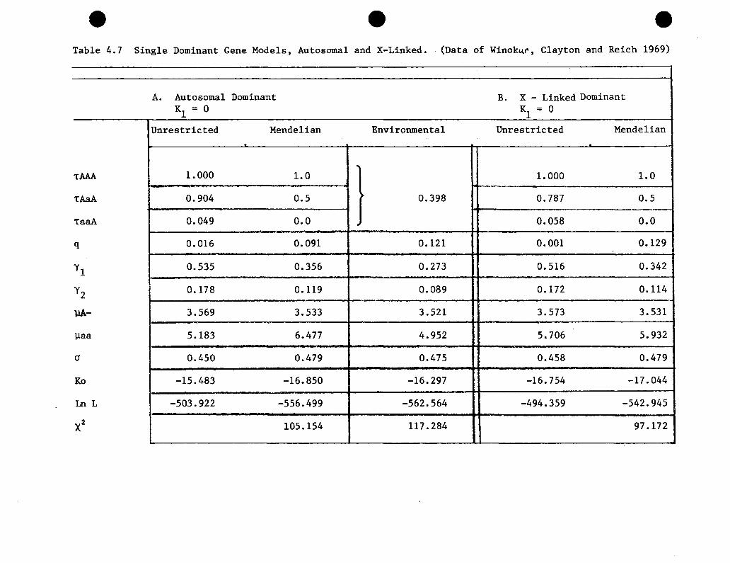
e e eTable 4.7 Single Dominant Gene Models, Autosomal and X-Linked. (Data of Winok~r, Clayton and Reich 1969)

A. Autosomal Dominant B. X - Linked DominantK = 0 K = 01 1

Unrestricted Mendelian Environmental Unrestricted Mendelian.

,TAAA 1.000 1.0 1.000 1.0- ,.......

TAaA 0.904 0.5 0.398 0.787 0.5

TaaA 0.049 0.0 . 0.058 0.0

q 0.016 0.091 0.121 0.001 0.129

Yl 0.535 0.356 0.273 0.516 0.342

Y2 0.178 0.119 0.089 0.172 0.114

llA- 3.569 3.533 3.521 3.573 3.531

llaa 5.183 6.477 4.952 5.706 5.932

(J 0.450 0.479 0.475 0.458 0.479

Ko -15.483 -16.850 -16.297 -16.754 -17.044

LnL -503.922 -556.499 -562.564 -494.359 -542.945

X2 105.154 117.284 97.172

118

Table 4.8 Two-gene models(Data of Winokur, Clayton and Reich 1969)

Double Dominant Heterogeneity Winokur 1970

qB 0.170 0.129 0.161 For all models,

qA 0.176 0.000 0.200transmission prob-abilities for both

Y1 0.633 0.339 0.585 loci are fixed at

Y2 0.211 0.113 0.190 their Mendelianvalues.

III 3.544 3.522 3.472The alleles A,a are

112 7.0 7.0 7.461 at autosomal locus

113 7.0 and the alleles B,bare at an X-linked

(J 0.484 0.463 0.461 locus.KO -16.223 -16.428 -16.217

1n L -533.707 -542.926 -534.448

Double dominant: Heterogeneity: Winokur (1970):

IlAAB· , IlAAB • , IlAABB IlAAB • ,

IlAaB· , IlAaB· , IlAaBB IlAaB • ,= III llaaB • , llaaBB = III

IlAABb IlAABb IlAABbIlAaBb = III Il

"aaB~} _aaB· ,IlAAb· , IlAAbb llaaBb llaaBb - 11 2PAab· , IlAabb IlAab· , IlAAbb IlAAb· , "MbjIlaab· , Ilaabb 112

IlAab·' IlAabb IlAab· , IlAabb =llaaB· , llaaBB

11 3Ilaab· , Ilaabb 11 2

Il aab· , IlaabllaaBb =

CHAPTER V

ANALYSIS OF THE DATA OF GOETZL ET. AL. (1974)

5.1 Description of the data.

The families analyzed in this Chapter were reported by Goetzl

et. ale (1974). The probands are from a series of patients admitted

consecutively to the Dartmouth Hitchcock Mental Health Center

between August 1968 and July 1971 who had a discharge diagnosis of

manic depressive illness, manic phase. There are 39 probands (20

female, 19 male) in 38 families; two of the probands are sisters.

Information on first degree relatives was obtained by sending a

questionnaire to all living relatives over 15 years old. Direct infor­

mation was obtained on 119 of 155 living first degree relatives (76%).

Information on others, and on dead relatives, was obtained from the

proband and hospital records, if any. The families in most cases

consist of two or three generations. In a few families there is also

information on aunts, uncles, and grandparents. There is no information

on spouses. Age at examination is recorded for about 90% of the people

with unknown ages estimated as in section 3.1. Nearly all of those

with unknown ages are relatives more distant than first degree. Age of

onset is recorded for 55 of 71 affectively ill people.

There are a total of 321 individuals in the 38 families, 157

(48.9%) males and 164 (51.1%) females. The probands have an average of

6.3 first degree relatives (7.5 for female, 5.1 for males). The

120

average size of the proband's sibship is 2.0 (2.2 for female, 1.9

for male). Of the 19 probands (10 female, 9 male) who have children,

the average number is 2.6 (2.7 for females, 2.4 for males). Both male

and female probands have an approximately equal number of brothers

and sisters, and of sons and daughters.

Among the affectively ill people sex ratios are shown in Table 5.1.

Table 5.1 Sex ratios among affectively ill people.(Data of Goetzl et. al. 1974)

Female Male Total

All affectively ill 40 (0.563) 31 (0.437) 71

All ill, excluding probands 20 (0.625) 12 (0.375) 32

Manics 22 (0.524) 20 (0.476) 42

Manics, excluding probands 2 (0.667) 1 (0.333) 3

Depressives 17 (0.630) 10 (0.370) 27

All affectively ill plus alcoholics 42 (0.506) 41 (0.494) 83

All affectively ill plus alcoholics 22 (0.500) 22 (0.500) 44excluding probands

Depressives plus alcoholics 19 (0.487) 20 (0.513) 39

None of the ratios are significantly different from 0.50 at the

5% level, but the trends are the same as in other studies: there is

an excess of women among all affectively ill people, with the excess

due to those with depression only, and equal numbers of men and women

among those with mania. Counting alcoholics as affectively ill

results in approximately equal numbers of men and women in all

categories.

121

Age of onset was recorded for 55 affectively ill people and

some characteristics of the distribution are shown in Table 5.2.

Among all affectively ill people, the average age of onset is 32.7,

with a standard deviation of 13.1, and the distribution is signifi­

cantly positively skewed. The minimum age of onset is 15 years, the

maximum 72 years. One-third of all ill people are affected by age

25, half by 32, and two-thirds by 40.

There are no significant differences between the age of onset

distributions of males and females, probands and other affectively

ill people with mania and those with depression only (Kolmogorov­

Smirnov 2-sided p>0.25 in all cases). As in other studies, people

with mania tend to have earlier onset than those with depression only,

but in this study the difference is not significant.

The empirical age of onset distribution was compared with the

best fitting normal, lognormal, squareroot normal, (l/onset) normal,

and exponential distributions. The plots of the major distributions

considered, the normal, lognormal, and exponential, are shown in

Figures 5.1 and 5.2. Of the distributions considered, the lognormal

distribution provides the best fit for the age of onset distribution

in these data, with a mean of the log ages 3.4 and variance 0.029.

In all further analyses it will be assumed that age of onset is

approximately log normally distributed.

The distribution and diagnoses of affectively ill first degree

relatives is shown in Table 5.3. There is male to male transmission

in four of the families, while the general level of risk to relatives

is comparatively low (see Table 5.4). Sixteen of the probands

:T------------~::::;c:::::===~=,

lognormal

O-l""=-~-I--_,---_r---_r_---r_--__t---_l

· 10.0 20.0 30.0 'l0.0 50.0 60.0 70.0 80.0AGE OF ONSET

Figure 5.1 Age of onset with best fitting normal and lognormaldistributions. Goetzl et. ale (1974).

122

Figure 5.2 Age of onset with qest fitting exponential distribution.Goetzl et. ale (1974).

- x~•

!8co0

!"Z

I.~=

5......i~••~

~10.0 20.0 30.0 'l0.0 50.0 60.0 70.0 10.0

IlG£ Of ONSET

123

Table 5.4 Weinberg age-corrected morbidity risk~ foraffective illness. (Goetzl et. al. (1974)

Female Proband Male Proband

Mother 24.2% 18.5%

Father 18.8 12.5

Sister 27.0 9.1

Brother 2.2 10.0

Daughter 57.1} very small 76.9

{Son 28.6 numbers 57.1

(9 female and 7 male) have no affective illness in their first degree

relatives. Other illnesses in the family include alcoholism, two cases

of schizoaffective disorder, and one case of schizophrenia.

The proportion of all affectively ill who are probands, by

decade of onset, is shown in Figure 5.3. The best fitting curves of

form KO+Kl (In a) + K2 (ln a)2 = In p and K~+K~(ln a) = In p are also

plotted. The proportions are not significantly heterogeneous among

2age classes (X4 = 1.181, p>0.5). A constant ascertainment function

is probably adequate for these data. This hypothesis will be tested

in section 5.2.1.

5.2 Segregation Analyses.

5.2.1 Single gene models

As explained in section 2.1.4, the single gene models to be

examined are a single autosomal gene, and a single X-linked gene. The

data are analyzed first with alcoholics counted as normal, and then

with alcoholics counted as affected with z=l. For the preliminary,

Figure 5.3 Proportion of affectively ill people who are probandsby decade of onset. Goetzl et. al. (1974).

1

124

p

o

-!'" .. ....- ..- ..--'- ... --~ - ---,

".......

10 20 30 40Age of onset (a)

50 60

--- In p = -1.5 + 0.8 (In a)

--- In p = 0.2 - 0.2 (In a)

20.2 (In a)

Vertical lines indicate ± standard error.

125

exploratory runs, the transmission probabilities are fixed at their

Mendelian values. Under these conditions, the models examined under

each of the autosomal and X-linked hypotheses are a three mean model

(ll • II ,ll all distinct, corresponding to a " codominant" gene A)AA Aa aa

and a two mean model (llAA=llAa' corresponding to a "dominant" gene A),

with ascertainment either a linear or a constant (Kl=O) exponential

function of age of onset. Results of these runs are shown in Table

5.5 and 5.6.

Neither the hypothesis that Kl=O, nor the hypothesis that llAA=llAa

can be rejected under either the autosomal or the X-linked model,

whether or not alcoholics are counted as affected. Therefore, in all

further analyses it is assumed that llAA=llAa and Kl=O. Furthermore, in

both the autosomal and X-linked cases, the likelihoods are much higher

when alcoholics are considered normal. Since there is no information

on age of onset of alcoholism, subsequent analyses assume that

alcoholics are normal.

The X-linked and autosomal models with alcoholics considered

normal are strikingly similar. The likelihoods are very close: the

ratio of the likelihood of the autosomal to the X-linked model is

about 3.3. With the exception of the. gene frequency, which is higher

assuming an X-linked model, the estimates of the parameters are nearly

the same. Under a simple Mendelian hypothesis, these data do not

discriminate very well between the X-linked dominant and autosomal

models.

Table 5.7 shows the results of testing the Mendeliam

TAA A=l.O. TAa A=O.5. Taa A=O.O) and environmental

126

(H : T =T =T ) hypotheses under the X-linked and autosomalo AA A Aa A aa A

dominant models. Both hypotheses are rejected with p<O.OOl. The

environmental model is more likely than the Mendelian model for both

autosomal and X-linked genes, but the environmental model is also much

less likely than the unrestricted model.

Under the autosomal dominant Mendelian model, the means of the

f d ·"b" d 3.461 31 8 dage 0 onset 1str1 ut10n correspon to e =. years an

e5 . 035=153.7 years. Two standard deviations below the upper mean is

(5.035-2xO.494) 57 2 th t "f 1 "h te = . years, so a a port1on 0 peop e W1t geno ype

aa live long enough to develop manic depressive illness. A similar

situation exists under the X-linked dominant Mendelian model: the means

3.461 31 8 d 4.790 120 3 " h d d d "are e =. years an e = . years W1t two stan ar eV1a-

" b 1 h d" (4.790-2 x 0.538) 41 0tlons e ow t e upper mean correspon 1ng to e = .

years. If we want a model in which there are no such "sporadic" cases,

one approach is to fix the upper mean at some age large enough so that

no ones lives long enough to become affected. The results when ~aa

is set at 7.0 are shown in Table 5.8. Doing this makes very little

difference in the likelihoods or the estimates of the parameters, and

both the Mendelian and environmental hypotheses are rejected with

p<O.OOl, for both X-linked and autosomal models. Further manipulations

of single gene models seem unwarrapted, and it appears that neither

an autosomal nor an X-linked Mendelian model can account for transmis-

sion of affective illness in these data.

5.2.2 Two gene models

The two gene models examined in detail are the heterogeneity model,

and the double dominant model (see Table 2.1). Results of these

127

analyses are shown in Table 5.9. Transmission probabilities are fixed

at their Mendelian values for both loci and the upper mean is fixed

at 7.0. For the double dominant model, the gene frequencies are

similar to those in the single gene models (compare with columns 2 and

5 of Table 5.9), and all other estimates are similar. For the hetero­

genity model, the frequency of the X-linked gene is much lower than

that of the single gene X-linked model but all other estimates are

similar. In both cases the likelihood of the two-gene models is only

slightly higher than the likelihood of either single-gene model.

There is no point in formally testing the Mendelian or environmental

hypotheses. Since the likelihoods under the two-gene model must be

larger than the likelihoods under the corresponding single gene models,

these hypotheses will necessarily be rejected.

These are just two of the many possible two-gene models. While

it is conceivable that there is a two-gene model that will fit these

data, it seems fruitless to search for it.

5.3 Conclusions.

In their analysis of these data, Goetzl et. al. (1974) conclude

that "any gene locus that exists on the X chromosome is not itself a

sufficient or necessary condition for the transmission of manic

depressive illness". They base this conclusion on their findings that

there is no significant difference in morbid risks to fathers and

mothers of either male or female probands, that the overall sex ratio

of affectively ill people is one to one, and that there are four ill

son-ill father pairs in the 38 families. The analysis presented in

this Chapter supports their conclusion that an X-linked gene cannot

128

explain the illness patterns in these families, and indicates that

a single autosomal gene is also an untenable model. There is no

reason to prefer either an X-linked or an autosomal model; when the

variable age of onset and ascertainment via probands is taken into

account both models fit equally poorly. Consideration of two genes

simultaneously does not help: the two-gene models examined also give

a very poor fit. It should be noted that the environmental models

of no vertical transmission of manic depressive illness also do not

fit. It may well be that there is some kind of genetic transmission

in these families, but it is too complex to be explained by the

models examined here.

129

Table 5.2 Age of onset. (Data of Goetz1 et. a1. 1974)

Number of StandardObservations Minimum Maximum .Mean Deviation Skewness

All affectively 55 15 72 32.7 13.1 0.72*ill

Males 26 15 58 32.1 12.4 0.48

Females 29 16 72 33.2 13.8 0.84*

Probands 39 15 57 31.4 11. 7 0.52

Manics 41 15 57 31.8 11.6 0.44

Depressives 10 19 72 38.7 17.5 0.64

*Significantly greater than 0, p<0.05

Table 5.3 First degree family hisotry. (Data of Goetz1 e1. a1. 1974)

Female Proband Male Proband

Mo Fa .Sis Bro Dau Son Mo Fa Sis Bra Dau Son

Depression 3 2 4 3 4 2 3 1 0 1 4 1

Mania 1 0 0 0 0 0 0 1 0 0 1 1

All affective 4 2 4 3 4 2 3** 2 0* 1 5 2ill

Totab15 years 19 19 2a 17 13 14 19 19 18 16 13 7

*1 sister was diagnosed as schizoaffective.

**1 mother was diagnosed as schizoaffective.

Table 5.5 Preliminary autosomal models. (Data of Goetzl et. al. 1974)

A. Alcoholics = Normal B. Alcoholics = Affected (z=l)

Linear Ascertainment Constant Ascertainment Linear Ascertainment Constant AscertainmentCodominant Dominant Codominant Dominant Codominant Dominant Codominant Dominant

q 0.151 0.145 0.134 0.140 0.233 0.227 0.209 0.182Y1 0.260 0.260 0.268 0.263 0.336 0.328 0.349 0.355YZ 0.072 0.072 0.074 0.073 0.067 0.066 0.071 0.071

IlAA 3.310 } 3.442 3.379 } 3.461 3.173 } 3.486 3.208 } 3.494IlAa 3.440 3.471 3.582 3.575Il aa 5.070 5.070 5.070 5.035 5.846 5.871 5.140 5.079

a 0.488 0.488 0.488 0.494 0.495 0.498 0.491 0.493K

O -2.494 -2.170 -1.489 -1.489 -2.505 -2.368 -1.430 -1.454Kl 0.285 0.203 0 0 0.293 0.255 0 0

In L -212.792 -212.838 -213.016 -213.038 -230.440 -230.907 -230.825 -231.154

Transmission probabilities are fixed at their Mendelian values. All hypotheses tested assumingalcoholics are normal.

(1) HO: Kl=O for dominant model xi = 0.400 } p>O. 50

codominant xi = 0.448

2}(2) HO: IlAA=IlAa when Kl=O, Xl = 0.044 p>0.50 ~

w2 0

when KIf0, Xl = 0.092

e e e

e e e

Table 5.6 Preliminary X-linked models. (Data of Goetzl et. al. 1974)

A. Alcoholics = Normal B. Alcoholics = Affected (z=l)

Linear Ascertainment Constant Ascertainment Linear Ascertainment Constant AscertainmentCodominant Dominant Codominant Dominant Codominant Dominant Codominant Dominant

I

q 0.322 0.333 0.276 0.250 0.325 0.326 0.296 0.357Yl 0.211 0.221 0.230 0.255 0.187 0.188 0.190 0.207Y2 0.062 0.062 0.065 0.074 0.037 0.037 0.038 0.042

~AA 3.340 } 3.419 3.349 } 3.461 3.076 } 3.068 3.098 } 3.230~Aa 3.364 3.451 3.052 3.068

~aa 4.571 4.480 4.626 4.790 3.791 3.791 3.813 3.944

0 0.490 0.497 0.489 0.538 0.260 0.260 0.260 0.345KO -2.353 -2.424 -1.430 -1. 423 -2.591 -2.587 -1.442 -1. 448K

l 0.253 0.269 0 0 0.320 0.318 0 0

In L -213.596 -213.898 -213.828 -214.222 -230.717 -230.733 -230.952 -232.642

Transmission probabilities are fixed at their Mendelian values. All hypotheses are tested assumingalcoholics are normal.

(1) HO: Kl=O when ~AA=~Aa2

Xl = 0.648

when ~AA:!:~Aa2Xl = 0.464

(2) HO: ~AA=lJAa when Kl=O xi = 0.788p>0.50

when Kl:!:O2

Xl = 0.604~w~

Table 5.7 Single gene dominant models: Autosomal and X-linked. (Data of Goetz1 et. al. 1974)

Autosomal X-linked

Unrestricted Mendelian Environmental Unrestricted MendelianTAM 1.000 1.0 1.000 1.0TAaA 0.996 0.5 l

0.639 0.999 0.5J

TaaA 0.044 0.0 0.101 0.0

q 0.006 0.140 0.023 0.015 0.250

Y1 0.589 0.263 0.237 0.534 0.255

Y2 0.164 0.073 0.066 0.151 0.074

]JA- 3.600 3.461 3.563 3.480 3.461]Jaa 5.476 5.035 4.801 5.179 4.790

0 0.467 0.494 0.492 0.436 0.538KO -1. 455 -1. 489 -1.446 -1.413 -1. 423

lnL -177.139 -213.038 -196.849 -186.079 -214.2222

71. 798 39.42 56.286X --- ---

- - e

~WN

e e e

Table 5.8 Single gene moce1s with ~ fixed at 7.0: Autosomal and X-linked.aa(Data of Goetz1 et. al. 1974)

A. Autosomal B. X-linked

Unrestricted Mendelian Environmental Unrestricted Mendelian

LAAA 1.000 1.0 1.000 1.0

LAaA 0.998 0.5 } 0.531 0.998 0.5

LaaA 0.038 0.0 0.103 0.0

q 0.006 0.149 0.005 0.169 0.422

'VI 0.705 0.264 0.302 0.733 0.230

'V2 0.181 0.073 0.084 0.209 0.060

~A- 3.762 3.548 3.679 3.787 3.525

~aa 7.0 7.0 7.0 7.0 7.0(J 0.536 0.518 0.558 0.549 0.512KO -1.439 -1.498 -1. 454 -1. 385 -1. 448

In L -177.372 -213.429 -199.567 -184.078 -215.0372

72.114 22.195 61. 918X --- ---

.....ww

134

'!';lblc 5.9 Two-locus models. (Data of Goetzl et. al. 1974)

---------------

Double dominant Heterogeneity

0.520

0.168

0.350

0.097

3.536

0.058

0.122

0.255

0.071

3.510

For both models, trans­mission probabilities arefixed at their Mendelianvalues for both loci,11

2=7.0, and K

1=K

2=0.

B is X-linked and A isautosomal.

7.0 7.0

() 0.519 0.508

-I. 483 -1. 489

III L -212.541 -213.152

Double dominant: Heterogeneity

IlAABB \IJAaBB i

IIl aaBB I11 AABb \IlAaBb

~JaaBb

IlAAbbIJ

Aahb

IlAaB ' ,

lIaaB · ,

~laaBB"-

\Il aaBb

I Il AAb · ,(1l<l,IBb I lJ 2 PAah · ,,IlAAbh III AAb · ,

Il Aah · , 11 Aabh

lIMI~B' ,II

A,I1L,

CHAPTER VI

ANALYSIS OF THE DATA OF STENSTEDT (1952)

6.1 Description of the data.

The data in this chapter were reported by Stenstedt (1952). The

probands are all cases of "manic depressive psychosis" who were

hospitalized in northwest Sweden during the years 1919-1948.

Stenstedt's definition of manic depressive illness includes both

cases of unipolar depression and bipolar manic depression. Probands

were ascertained using registers from state asylums and population

registers. Stenstedt personally interviewed the probands and many

of their first degree relatives. Probands and their families were

followed up until the end of the study in 1948. The original data

consist of 201 families. Of these, 51 have mania in a proband and

are used here. There are 54 probands in these 51 families, 30 female

and 24 male.

The diagnosis for the probands was the hospital diagnosis, and

was confirmed by Stenstedt by a chart review. The diagnosis of

relatives was based on symptomo10gy and social factors, and was

obtained from hospital records and/or personal examination when

possible, and information from relatives when records were unavailable

or personal examination impossible. Secondary cases (those other

than probands) were called "certain" if confirmatory hospital records

136

were available or the relative was personally diagnosed as affectively

ill by Stenstedt; they were called "uncertain" otherwise.

Diagnoses of mental illness were made on the basis of criteria

such as the following. Manic depressive disease was diagnosed if

the disease showed marked depressive or manic symptoms with poor

social functioning during episodes, but good functioning between

episodes. Schizophrenia was the diagnosis if the disease was

chronic and left "marked alteration of personality". A "cycloid

psychopath" had marked mood swings which were not severe enough to

be disabling. "Psychopathy" was a rather vague category applied to

a relative who was described as abnormal, but with no specific

details available, and who was not severely enough disabled to fit

into one of the other categories. Other diseases present in the

families include alcoholism, mental defects, senile and presenile

psychoses, and epilepsy.

There are a total of 549 individuals in 51 families. The data

consist of the proband, his parents, children and sibs. These are

thus simple, 2- and 3-generational pedigrees. The data include

the age of "disapperance from observation" (ie. age at the end of

the study, or death, or age at which a person's family lost track

of him) for nparly everyone, the number and type of episodes for

;It'fectively ill people, and description of "uncertain" cases. The

families are fairly large: the average size of the proband's

sibship is 6.8. Of the 33 probands who had children, the average

family size is 3.3.

137

The overall sex ratio is 267 female (48.6%): 282 male (51.4%).

Among probands it is 44.4% male: 55.6% female; this is not signif­

2icantly different from 1:1 (X

l=0.677, p>0.25). Female probands have

significantly more sons than daughters (37 sons, 15 daughters,

2xl=9.3, p<O.Ol). but a similar difference is not present among

children of male probands. Both female and male probands have

approximately equal numbers of brothers and sisters.

There are a total of 76 affectively ill people (using a fairly

broad definition of "ill"--those who are designated "uncertain" cases

are included). The sex ratios are shown in Table 6.1. None of the

ratios differs significantly from a one-to-one sex ratio. There is,

however, an excess of women among all affectively ill, which is due

mainly to those who have unipolar depression only. When alcoholics

are included as affectively ill, the excess of women disappears.

The age of onset distribution is very similar in females and

males, and in probands and other affectively ill (see Table 6.2).

People with mania tend to have an earlier onset than those with

depression only (Kolmogorov-Smirnov statistic = 0.39; 2 sided p<O.Ol).

Age of onset was recorded for 74 of 76 affectively ill people. The

range was 14-72 years with mean 33 and standard deviation 13.4. The

median age of onset was 29, with one third affected by age 25, and

two thirds by 36. In general, the distributions for various break-

downs show positive skewness. The best fitting exponential, normal,

-1lognormal, squareroot normal, and (age of onset) normal were

compared to the empiric age of onset distribution. The lognormal

is the best fitting of the distributions, although there is not

138

much difference between the fits of the lognormal and exponential

distributions (Figures 6.1 and 6.2). For further analyses, it will

be assumed that age of onset is lognormally distributed.

In his original paper Stenstedt reported morbidity risks (age

corrected by the abridged Weisberg method using a risk period of

15-60 years) of

12.28% + 1.36 to sibs of probands

7.35% + 1.34 to parents, and

9.40% + 2.39 to children

(counting both "certain" and "uncertain" cases as affected). He

found no significant differences in risk between sexes, between

families of probands with "few attacks" (less than 3) and "several

attacks" (3 or more), or between families in which the proband had

mania and those in which the proband had depression only. Thirty-

three probands (19 female. 14 male) had no first degree relative

with affective illness. See Table 6.3 for a more complete breakdown

of first degree family history.

The proportion of affectively ill people who are probands as a

function of age of onset is shown in Figure 6.3, along with the best

2fitting curves of the form In p = K

O+ K

l(In a) + K

2(ln a) and

In p = KO+ Ki(ln a). The proportions are not significantly hetero-

2geneous among age classes (X

S=1.58, p>0.5). A constant ascertainment

function is probably adequate for these data. The hypothesis that

K = K = 0 will be tested in section 6.2.1 2

139

•g

10 50flOE OF ONSET

60 70 10

Figure 6.1 Age of onset and best fitting normal and lognormaldistributions. Stenstedt (1952).

Figure 6.2 Age of onset and best fitting exponential distribution.Stenstedt (1952) •

..,...--------------------:--;---'"'V"---,~o

·~-tlr-O-.o~..:.--r----r-----r-----r----r---..,..----420.0 ao.o '0.0 . 50.0 10.0 0.0 10.0

IIGE OF ONSET

140

Figure 6.3 Proportion of affectively ill people who are probands,by decade of onset. Stenstedt (1952).

1

..

..--------T

-~rtfl !I I I 11

I I I I '

oL __L. ~.L. __ .I __ .. J--J J L.-+-_10 20 30 40 50 60 70 80

Age of onset, a

p

--- In p -0.5 + 0.04 (In a) - 0.01 (In a )2

~- In p -0.6 + 0.1 (In a)

Vertical lines indicate ± standard error.

141

6.2 Segregation Analysis.

6.2.1 Single gene models

Preliminary analyses on these data were performed under an

autosomal and an X-linked model, assuming the transmission prob-

abilities are fixed at their Mendelian values of TAAA

= 1.0,

TAaA = 0.5 and TaaA = O. Results for the autosomal gene are shown

in Table 6.4. A constant ascertainment function is adequate since

HO

: Kl

= 0 cannot be rejected (p>0.5), and allowing the age of onset

distribution to be a mixture of three lognormal distributions is not

significantly better than a mixture of two (p>0.5). Therefore for

subsequent analyses under an autosomal model it will be assumed that

KI

= 0 and ~AA = ~Aa· A comparison of parts (A) and (B) of Table 6.4

shows that the likelihoods are much larger when alcoholics are

considered normal than when they are considered affected (with z-l)~

There is no information on age of onset of alcoholism, so no further

runs will be done considering alcoholics as affected.

Under the autosomal model chosen for further analysis (i.e.,

dominant with constant ascertainment and alcoholics considered normal),

the means of the age of onset distribution correspond to an "affected"

3.636 5 927mean of e =37.9 years and an "unaffected" mean of e· =375 years.

Three standard deviations below the upper mean corresponds to 92 years

so that very few people with genotype aa live long enough to become

affected. The model is thus of a dichotomy between genetically

susceptible people with genotypes AA and Aa, and genetically unsus-

ceptible people with genotype aa. The frequency of gene A is large

enough (0.126) so that homozygotes are not rare among affected

142

people. The susceptibilities are quite low, however. Only 0.113 +

0.050 = 16.3% of individuals are expected to develop the disease if

they live long enough, in spite of the high mean age of onset for

aa people. The model is thus of a fairly common dominant gene with

low penetrance.

Table 6.5 shows results of the preliminary analyses assuming

an X-linked gene. It is assumed that alcoholics are normal, since

under the autosomal model the likelihoods were so much higher when

this is assumed. Again, the hypothesis that Kl

o cannot be rejected

for either a codominant or a dominant model and the hypothesis that

~ = ~ is not reJ·ected.AA Aa

and ~AA= ~Aa·

Therefore it will be assumed that KI = 0

The most striking feature of the X-linked models is the high

gene frequency (0.740 for the model chosen). An attempt was made to

look for other local maxima with lower gene frequencies and higher

susceptibilities, but none with a larger likelihood was found. The

susceptibilities are very low: only 10.2% (0.070 + 0.032) of

individuals are expected to develop manic depressive illness if they

live long enough. The means of the age of onset distribution cor-

respond to an affected group with genotypes AA or Aa and mean

e3

. 564=35.3 and an unaffected group with genotype aa and mean

e 5 . 920=372. Three standard deviations helow the upper mean is 108

years, so virtually no one with genotype aa lives long enough to he

affected. The X-linked model is therefore of a very common dominant

gene with low penetrance.

143

A comparison of Tables 6.4 and 6.5 shows that these data do not

discriminate between the models of an X-linked and an autosomal gene.

The difference in log likelihoods is 0.859, indicating that an X-

linked model is about 2.4 times as likely as the autosomal. With

the exception of the gene frequency, estimates of the parameters

are also quite similar under the two models.

Table 6.6 shows the results of testing the Mendelian and

environmental hypotheses under the autosomal and X-linked models.

For both the X-linked and the autosomal models the Mendelian

hypothesis is rejected (p<O.OOOl). Since under the unrestricted

model LaaA converges to the bound 1.0, the degrees of freedom of

2the X 's are reduced to between 2 and 3 for the Mendelian hypothesis

and to between 1 and 2 for the environmental.

Under the autosomal model the environmental hypothesis is not

rejected (p>0.20). The segregation patterns in these families

cannot be explained by a single gene, either autosomal or X-linked;

it is more likely that transmission is entirely environmental.

6.2.2 Two gene models

Two different models assuming one X-linked dominant and one

autosomal dominant were examined. See Table 2.1 for the genotype-

phenotype correspondences. Table 6.7 shows the results of the

analysis. The double dominant model is quite similar to the single

gene autosomal and X-linked models. The X-linked gene in the

heterogeneity model has a much lower gene frequency but otherwise the

estimates are similar. The likelihoods of both two gene models,

the single gene autosomal, and the single gene X-linked models are

144

all quite similar. There is no point in testing the Mendelian

hypothesis for the two gene models since it would necessarily be

rejected. Thus these two gene models are also inadequate for

explaining the genetic transmission of manic depressive illness in

these data.

6.3 Conclusions.

Stenstedt's (1952) analysis of these data included all 201

families with both unipolar and bipolar probands. He found, however,

that there were no significant differences in morbid risks to first­

degree relatives between unipolar and bipolar probands. Based on the

segregation patterns Stenstedt concludes that the mode of inheritance

cannot be exactly determined but that some kind of dominant trans­

mission, probably an autosomal gene with incomplete penetrance, is

likely.

The analysis in this Chapter provides no support for a single

gene hypothesis, either autosomal or X-linked. The two gene models

examined are no more likely than the single gene models. If there

is a genetic mechanism operating in these families it is too complex

to be detected by the one-or two-locus models considered in this

Chapter. The environmental model provides a better explanation of

the illness pattern than any of the genetic models. It could be that

the phenotypic variability caused by genetic factors is too small in

comparison to the environmentally caused variability to be picked up

by these models. Another possibility is that there is a good deal of

gene.tic heterogeneity among families so that no single genetic

mechanism can be detected.

Table 6.1 Sex ratios among affectively ill people.(Data of Stenstedt 1952)

Females Males Total

All affectively ill 42 (0.553) 34 (0.447) 76

All affectively ill +42 (0.483) 45 (0.517) 87alcoholics

All affectively ill, 12 (0.545) 10 (0.455) 22excluding probands

All affectively ill, excluding 12 (0.387) 19 (0.613) 31probands,+ alcoholics

Unipolar depressives 11 (0.579) 8 (0.421) 19

Unipolar depressives 11 (0.324) 17 (0.676) 28+ alcoholics

Bipolar manic-depressives 31 (0.544) 26 (0.456) 57

Table 6.2 Age of onset.(Data of Stenstedt 1952)

N Min Max Mean Std. dev. Skewness

All affectively ill 74 14 72 33.0 13.4 0.88**

Males 34 16 72 32.8 14.3 1.10**

Females 40 14 65 33.3 12.8 0.66*

Probands 54 14 65 32.4 12 .5 0.83**

Bipolars 56 14 72 30.6 12.5 1.18**

Unipolars 18 18 65 39.4 13.7 0.38x

Significantly different from 0 *p<.05 **p<.Ol

xSample too small to detect significance.

145

Table 6.3 First degree family history.(Data of Stenstedt 1952)

146

Female Probands Male ProbandsMo Fa Sis Bro Dau Son Mo Fa Sis Bro Dau Son

Depression 2 1 1 2 0 0 1 0 1 0 0 0

Uncertain 1 1 0 1 0 0 0 1 2 2 0 0depression

Mania + 1 0 1 2 0 1 0 0 1 1 0 0depression

Total affective1y 4 2 2 5 0 1 1 1 4 3 0 0ill

Total number 15 36 32 80 78 18 42 24 24 56 51 9 41or older

e - e

Table 6.4 Preliminary autosomal models. (Data of Stenstedt 1952)

A. Alcoholics = Normal B. Alcoholics = Affected

Linear Ascertainment Constant Ascertainment ~A~~~Aa Linear Ascertainment Constant AscertainmentCodominant Dominant Codominant Dominant ~1 =7.0 Codominant Dominant Codominant Dominant

aa

q 0.221 0.219 0.237 0.219 0.191 0.380 0.373 0.373 0.339

Yl 0.096 0.094 0.093 0.094 0.097 0.112 0.112 0.112 0.115Y2 0.042 0.042 0.042 0.042 0.044 0.037 0.037 0.038 0.040

llAA 3.639 } 3.574 3.574 } 3.574 } 3.574 3.598 } 3.582 3.598 } 3.565llAa 3.555 3.574 3.565 3.565

~aa 5.820 5.830 5.786 5.830 7.0 5.748 5.748 5.748 5.718

(J 0.411 0.415 0.415 0.415 0.415 0.408 0.408 0.408 0.408KO -0.506 -0.433 -0.432 -0.433 -0.435 -0.420 -0.422 -0.422 -0.406Kl 0.006 -0.0002 0 0 0 -0.0003 -0.0005 0 0

In L -228.342 -228.404 -228.397 -228.406 -228.430 -247.304 -247.338 -247.305 -247.436

For all models, TAAA=I.O, TAaA=0.5, TaaA=O.O. All hypotheses tested assuming alcoholics are normal.

(1) HO: Kl=O for codominant xi=0.002

dominant xi=0.OI6

2(2) HO: ~AA=~Aa when KI=O X~=0.081

when KI~O Xl =0.067

I-'~".J

Table 6.5 Preliminary Single gene models: X-linked, Alcoholics = Normal.(Data of Stenstedt 1952)

7.0

o

0.070

0.032

0.743

0.410

-0.418

} 3.564

-228.232

Dominant-with constantascertainment and II =7.0aa

0.660 0.740

0.072 0.070

0.033 0.032

3.516 }. 3.5643.662

5.104 5.902

0.399 0.411

-0.419 -0.418

0 0

-227.947 -228.231

, A=O.Oaa.

p>.90

Constant AscertainmentCodominant Dominant

In all models 'AAA=l.O, 'AaA=0.5,

HO: Kl=O - for dominant X~=O.OlO}codominant Xi=0.002

2HO: llAA=uAa - for Kl=O Xl=0.568 } p>.40

Kl~O xr=0.597

Linear AscertainmentCodominant Dominant

q 0.652 0.743Yl 0.074 0.071Y2 0.033 0.032

llAA 3.527 } 3.564llAa 3.690

llaa 5.667 5.624(J 0.406 0.411K

O -0.349 -0.416K

l -0.024 -0.001

ln L -227.937 -228.226

f-'~(Xl

e e e

e e e

Table 6.6 Single gene dominant models: Autosomal and X-linked.(Data of Stenstedt 1952)

A. Autosomal B. X-linked

Unrestricted TIS Mendelian TIS equal Unrestricted . TIS MendelianT

AAA 0.00001 1.0 0.184 1.0T

AaA 0.995 0.5 } 0.454 0.428 0.5TaaA 0.535 0.0 1.000 0.0

q 0.064 0.126 0.055 0.096 0.740Y1 0.107 0.113 0.130 0.102 0.070Y2 0.050 0.050 0.061 0.048 0.032llA_ 3.649 3.636 3.649 3.633 3.564

llaa 5.868 5.927 5.920 5.780 5.902

a 0.436 0.468 0.436 0.427 0.411KO -0.414 -0.437 -0.413 -0.413 -0.418

1n L -213.355 -229.190 -213.931 -212.194 -228.2312

31.670X --- 1.152 --- 32.074

I-'-l::­\0

e

Table 6.7 Two locus models (Data of Stenstedt 1952)

Double dominant Heterogeneity

qA 0.181 0.108

qB 0.741 0.008

Yl0.111 0.110

Y20.051 0.049

)Jl 3.593 3.610

)J2 7.0 7.0

a 0.429 0.432

KO -0.437 -0.442

ln L -227.991 -228.691

Transmission probabilities are fixed at their Mendelianvalues for both loci, and )J2 is fixed at 7.0. qA is thefrequency of the autosomal gene and qB is the frequencyof the X-linked gene.

e e

f-'V1o

CHAPTER VII

LINKAGE ANALYSIS

7.1 Description of the family.

This Chapter presents segregation and linkage analysis on a large

family, to be referred to as the Lava family. The family was reported

by Winokur (1971) but has not been extensively analyzed.

The proband is a woman with bipolar manic depressive disease.

She has six brothers and three sisters. Both colorblindness and the

Xg blood group are segregating in this sibship. Figure 7.1 shows the

pedigree of the proband's first degree relatives. There is also

information on manic depressive disease status available on her aunts

and uncles, grandparents, first cousins, and the children of her sibs,

for a total of 76 individuals. Affective illness is present on the

maternal side of the proband's family: her maternal grandmother and

several first cousins have had depressions, a maternal aunt has had

manias and depressions, and three first cousins and an uncle are

alcoholic. There is no affective illness or alcoholism on the

paternal side.

This family is well suited for linkage analysis for several

reasons. There is a large sibship, and its members are old enough

to have passed through a large part of the risk period for manic

depressive illness. Both Xg and colorblindness are segregating, but

the family was not selected on the basis of two traits through the

82' , 76

not CB

~36L ,

+CB

~81 J46W44

not CB

54, I+

not CB

56, ,+

not CB

I-'VIN

CB Colorblind

Bipolar manic depressive illiness

Unipolar depression

Legend:

0 Male

0 Female

~or ~

_ or •,. . Proband

Not CB not colorblind

+ Xg (+) phenotype

Xg (-) phenotype

? Unknown affective illness phenotype

Numbers refer to age at examination

Numbers in parentheses refer to age of onset ofaffective illness.

Figure 7.1 Lava family: Pedigree of the proband's first-degree relatives.

e e e

153

proband. Ascertainment was through a manic depressive proband, and

examination of her sibs revealed brothers with colorblindnessand

brothers with the Xg phenotype. This avoids the problem of ascertain-

ment through "doubly ill" probands that apparently has been present

in other linkage studies on manic depressive illness (Gershon and

Bunney 1976). In addition, ascertainment corrections to the lod

scores will not be necessary. The corrections cancel out when the

lod score is formed since selection of the marker traits (Xg and

colorblindness) was done without reference to affective illness pheno-

types, and the analysis is not conditional on parental phenotypes.

The remainder of this Chapter will be in two parts. First, seg-

regation analyses are performed in order to find the best-fitting

single gene model. The parameters of this model when the transmission

probabilities are set at their Mendelian values are then used as input

for the linkage analysis.

7.2 Segregation analysis.

Both X-linked and autosomal models are examined, since other sets

of data seem to contain insufficient information to discriminate

between these modes of inheritance. Alcoholics are considered normal

and it is assumed that KI =K2=O. Table 7.1 shows the results under an

autosomal model. The codominant model is not significantly better

2than the dominant model (X

l=O.OI6, p>O.5), so the Mendelian and

environmental hypotheses are tested under the assumption that ~AA=~Aa.

Under these conditions, neither the Mendelian nor the environmental

hypotheses can be rejected, although the Mendelian model fits somewhat

hetter than the environmental model. The parameters of the Mendelian

Three standard

154

and unrestricted models are quite similar, with the exception of the

gene frequency which is larger under the Mendelian model. Under the

environmental model the gene frequency is much higher than under the

unrestricted or Mendelian models, and the susceptibilities are higher

as well, with little difference in the likelihoods. This indicates

that the likelihood surface is quite flat so that a wide range of

models with different parameter values will have similar likelihoods.

Table 7.2 shows segregation analysis under an X-linked model.

2The hypothesis that ~AA=~Aa is not rejected at the 1% level (X

l=4.652,

0.025<p<0.05). Since. in addition, under the codominant model,

~AA<~Aa it seems reasonable to assume that a dominant model is adequate.

Under the assumption that ~AA=~Aa' the gene frequency is small (0.008)

and the susceptibilities moderate (yl=0.41l and y

2=0.103). The mean

age of onset for people with genotypes AA and Aa is e 3 . 208=24.7 and

f 1 h h · 5.660 287or peop e wit genotype aa t e mean 1S e =.

deviations below the upper mean is 112 years, so that virtually no

one with genotype aa lives long enough to become affected. Therefore,

the most reasonable Mendelian X-linked model is one of a rare dominant

gene with incomplete penetrance and virtually no sporadic cases.

The last two columns of Table 7.2 are used to test the Mendelian

hypothesis. As with the autosomal model, this hypothesis cannot be

rejected. The estimates of TAaA and TaaA in the unrestricted model

are close to their Mendelian values. The estimate of TAAA

(0.476)

is not close to the 1.0 expected under a Mendelian model; however,

individuals of genotype AA are extremely rare (expected frequency

(0.0002)2) so this parameter is not well estimated in these data. The

155

likelihood surface is again quite flat, with ~ fairly wide range of

gene frequency and susceptibility estimates resulting in similar

likelihoods. Although the Mendelian model fits these data, it is

not reasonable to conclude that there is an X-linked dominant gene

for manic depressive illness segregating in the family. The hypothesis

of an autosomal dominant gene is not rejected, and these data do not

discriminate between these two modes of inheritance. The difference

in log likelihoods between an autosomal and an X-linked gene is only

1.60, indicating the X-linked model is about five times as likely as

the autosomal model. The data are ambiguous as to the mode of

inheritance of manic depressive illness. Linkage analysis may shed

some light on this matter.

7.3 Linkage analysis.

Lad scores are calculated assuming that the estimates obtained

under an X-linked dominant model are the "true" values (column 2 of

Table 7.2). The gene frequency for the Xg(+) allele is taken as 0.53

and that of colorblindness as 0.02 (Levitan and Montagu 1971), values

which are often observed in American caucasian populations. Table

7.3 shows the lod scores when the recombination fraction is equal

to 0.0, 0.1, 0.2, 0.3, and 0.4.

For purposes of comparison, lod scores for Xg are shown both

taking the variable age of onset of affective illness into account,

and assuming that the gene for affective illness is fully penetrant

and completely dominant (as has been assumed in other linkage analyses,

e.g. Mendlewicz and Fleiss 1974, Tanna and Winokur 1968). There is no

qualitative difference between these two cases: the maximum lod score

156

is positive and occurs a~ A = 0.0 in both cases. However, the lod

scores are considerably lower when the variable age of onset is taken

into account. This is to be expected since under the more complex

model genotypes cannot be determined with certainty, so the possibility

of sporadic cases and incomplete penetrance is allowed. Under the

simple model, the genotype of all brothers of the proband is certain,

and "recombinants" can be counted. Table 7.4 shows the phenotypes

of all persons on whom there is complete information. There is

complete association of phenotypes: all brothers are either Xg(+)

and normal, or Xg(-) and depressed. No such association of phenotypes

has been found in the population (Gershon and Bunney 1976). There

is thus some evidence (far from conclusive) for close linkage

between Xg and a gene for manic depressive illness in this family.

Lod scores for colorblindness are shown in the third column of

Table 7.3. All lod scores are negative, and increase with increasing

A. There is thus no evidence for linkage of manic depressive illness

and colorblindness in this family. Any suggestion of linkage between

manic depressive illness and colorblindness must be regarded with

some suspicion, in view of the association between these traits in

the population suggested by Gershon et. al. (1976).

7.4 Conclusions.

The results of this analysis provide some support for the

hypothesis that there exists a gene closely linked to the Xg locus

that leads to the development of manic depressive illness in some

families. The evidence is far from conclusive, however, and more

data need to be collected before a confident statement can be made.

157

Segregation analyses presented in Chapters III ~ VI suggest that such

a gene (if it exists) is not the most common mode of transmission of

manic depressive illness.

There is no suggestion of linkage with co1orblindness in this

family, as has been reported by Mendelewicz and his co1legues

(Mendlewicz et. a1. 1972, Mendlewicz and Fleiss 1974, Fieve et. al.

1973). However. there are a number of methodological problems in

those analyses, as pointed out by Gershon and Bunney (1976). The

most serious of these difficulties are that ascertainment corrections

were improperly applied, the analysis was appropriate for nuclear

families but was applied to multigeneration pedigrees in some cases,

and the variable age of onset and incomplete penetrance were not

taken into account. The conclusion of Mendlewicz and Fleiss (1974)

that a gene for manic depressive illness is closely linked to both

Xg and the colorblindness loci (protanopia and deutanopia) is

difficult to accept in view of the large distance between Xg and

the colorblindness loci (e.g. Levitan and Montagu 1971; see Figure 2.2).

In addition, the suggested population association (Gershon et. al 1976)

between colorblindness and manic depressive illness makes it difficult

to conclude anything about linkage. It is probably best to disregard

data on linkage between manic depressive illness and co1orblindness

until the association is better understood.

The analysis of linkage with Xg is less difficult since no

population association has been suggested. Gershon and Bunney (1976)

present a more conservative analysis of the data of Mendlewicz's

group, and find a smaller maximum lod score (1.88 instead of 2.95,

158

both at a recombination fraction of 0.2). This is still suggestive

of linkage, though not as strongly as reported by Mendlewicz and

Fleiss (1974). Gershon and Bunney (1976) point out that there are

still problems with their analysis, probably the most serious of

which is the crude way in which variable age of onset is taken into

account (unaffected people younger than 25 years were not counted).

The conclusions of linkage analysis on the Lava family are similar

to those of Gershon and Bunney (1976): there is a slight suggestion

of tight linkage with Xg. The variable age of onset is taken into

account, which results in lower lod scores than when manic depressive

illness is considered to be caused by a fully penetrant gene. If

the data of Mendelwicz and Fleiss (1974) were subjected to an analysis

similar to the one presented in this chapter, we would expect to find

lod scores lower than those previously reported, but probably still

positive.

There are some difficulties in the present analysis. Ideally,

the gene frequencies, susceptibilities, and age of onset distribution

parameters should be estimated simultaneously with the recombination

fraction. However, if this is done the ascertainment corrections

no longer cancel out when the lod score is formed, and computational

problems arise. Therefore, the parameters as estimated by segregation

analyses are assumed to be the "true" or population values. This is

probably not a serious limitation. The age of onset distribution

parameters are fairly stable over a wide range of models (see Chapters

III-VI), and different gene frequency estimates do not have much

effect on lod scores or estimates of A (Ott 1974).

159

There is complete information on affective illness and Xg types

on only five men in one generation of the Lava family. It would

be desirable to have the Xg types of the parents and daughters as

well. The analysis of the available data does not exclude the

possibility that there is an X-linked gene for manic depressive

illness in this family.

Table 7.1 Segregation analysis under an autosomal model.Lava family.

UnrestrictedMendelian Models TransmissionCodominant Dominant Probabilities; ~AA=~Aa

'AAA 1.0* 1.0* 0.902

'AaA 0.5* 0.5* 0.564

'aaA 0.0* 0.0* 0.000

q 0.006 0.013 0.001

Y1 0.392 0.396 0.354Y2 0.098 0.101 0.089

~AA 3.075} 3.227 } 3.216

~Aa 3.207

~aa 5.476 5.519 5.422

a 0.323 0.312 0.323K

O -16.753 -17.174 -16.813

In L -34.629 -34.637 -34.567

X2 --- 0.140

*FixedFor all Models K

1=K

2=0.

e e

EnvironmentalModel;~AA=~Aa

} 0.166

0.211

0.471--0.118

} 3.226

5.537

0.316

-16.821--

-36.245

3.356

-.....0'o

- e

Table 7.2 Segregation analysis under an X-linked model.Lava family.

e

UnrestrictedMendelian Models Transmission

Codominant Dominant Probabilities; ~AA=~Aa

TAAA 1.0* 1.0* 0.476

'AaA 0.5* 0.5* 0.607TaaA 0.0* 0.0* 0.000

q 0.0008 0.008 0.0002

Y1 0.401 0.411 0.390Y2 0.100 0.103 0.096~AA 3.620 } 3.208 } 3.205llAa 3.011

~aa 5.494 5.660 5.386

(J 0.173 0.313 0.309

KO -16.099 -17.457 -16.651

1n L -30.715 -33.041 -32.3622

1.358X ---*Fixed

For all Models, K1

=K2

=0. .....0\.....

Table 7.3 Lod scores for colorblindness and Xg.

Marker LocusRecombination Xg Xg Colorblindnessfraction (taking age of (ignorillg age of (taking age of onset

J- on into account) onset) into account)

0.0 0.497 1.204 -0.321

0.1 0.368 0.975 -0.177

0.2 0.239 0.720 -0.091

0.3 0.121 0.436 -0.038

0.4 0.033 0.149 -0.009

Table 7.4 Phenotypes of proband's brothers on whomcomplete information is available.

Brother* Xg Affective illness Colorblindness

1 + Normal not CB

2 + Normal CB

5 + Normal not CB

9 + Normal CB

10 - Depressed not CB

......0\

*Numbering is from left to right on Figure 7.1. N

- - e

CHAPTER VIII

SUMMARY AND CONCLUSIONS

The sets of data analyzed in Chapters III - VI came from several

different investigators who reached different conclusions about the

genetic basis of manic depressive illness. Stenstedt's (1952)

families come from a mostly rural area of Sweden about a generation

ago, and represent an attempt to identify and follow up all manic

depressive patients in the area over a fairly long period of time.

Most individuals were personally interviewed and diagnosed by

Stenstedt, and in spite of the relatively subjective nature of the

diagnoses, the criteria on which the diagnoses were based were quite

similar to the research criteria proposed by Feighner et. al. (1972)

for most psychiatric illnesses. The other three sets of families

(Helzer and Winokur 1974; Winokur, Clayton and Reich 1969; and Goetzl

et. al. 1974) are from this country and were collected within the last

ten years. The probands were from series of consecutive admissions

of manic patients to mental hospitals, and diagnoses for probands

and their relatives were based on the Feighner criteria. Helzer

and Winokur (1974) and Winokur, Clayton and Reich (1969) attempted

to personally interview all first-degree relatives using a structured

interview schedule, while Goetzl et. aI, (1974) sent out a

questionnaire. Information on more distant relatives was obtained

from the proband or his first-degree relatives.

164

The method of analysis used by these investigators was the

calculation of age adjusted morbidity risks to fathers, mothers,

brothers, and sisters, and the comparison of these risks to

segregation ratios expected on specific genetic hypotheses. Helzer

and Winokur (1974), and Winokur, Clayton and Reich (1969) concluded

that an X-linked dominant gene was responsible for manic depressive

illness; Stenstedt (1952) and Goetzel et. al. (1974) concluded that

an autosomal dominant gene was a more reasonable genetic model.

In spite of the differences in data collection methodology, some

characteristics of the sets of data were quite similar. The sex

ratios of affectively ill people showed a consistent trend of an

excess of women among all affectively ill, while the sex ratio among

those who had had mania was about one to one. When alcoholics were

considered affectively ill the sex ratio was also close to one to

one. The age of onset distribution for all affectively ill people

was well approximated by a lognormal distribution in all studies.

Bipolar people tended to have earlier onset than unipolars, but

there were no significant differences in age of onset between men

and women, or probands and other affectively ill. The range of onset

was about 15 to 70 years, with a mean of 32 years and standard

deviation of 14, and the distribution was significantly positively

skewed. Age of onset was thus extremely v~riable and skewed towards

younger onset.

Affective illness was definitely familial in all sets of data,

but the overall level of risk to first degree relatives varied

somewhat among studies, ranging from about 10% in Stenstedt's (1952)

165

data to about 25% in that of Winokur, Clayton and Reich (1969).

These differences are not surprising in view of the span of time

and space over which the data were collected. The studies also

varied in the amount of observed father to son transmission of

affective illness. Helzer and Winokur (1974) found one case

and Winokur, Clayton and Reich (1969) found none, while Stenstedt

(1952) and Goetzl et. ale (1974) found that father to son trans­

mission was not significantly rarer than father to daughter or mother

to son transmission. The different results obtained by different

investigators have so far been difficult to explain.

In view of these discrepancies, the segregation analyses

presented in Chapters III through VI are remarkably consistent

with regard to the conclusions drawn. A single gene model does not

fit, and the autosomal and X-linked models are equally poor. This

conclusion could be drawn only after a formal test of the Mendelian

hypothesis. In each set of data, however, for both the autosomal and

X-linked genes, a Mendelian model could be found that gave reasonable

estimates of the parameters. It is not surprising that investigators

assuming a single Mendelian locus, either autosomal or X-linked,

would conclude that the segregation patterns supported this hypothesis.

It is also not surprising that both X-linked and autosomal modes of

inheritance have been proposed. For the most part, if a Mendelian

model is assumed, the data do not discriminate very well between

these two modes of inheritance. In the data of Stenstedt (1952),

Helzer and Winokur (1974) and Goetzl et. ale (1974) the likelihoods of

the X-linked and autosomal Mendelian models are very similar. The

166

data of Winokur, Clayton and Reich (1969) is an exception: the

X-linked model has a much higher likelihood than the autosomal model

in these data.

The environmental model of no vertical transmission of manic

depressive illness was also rejected. This model sometimes had a

smaller likelihood than the corresponding Mendelian model, and some­

times a larger likelihood. The only data in which the environmental

hypothesis was not easily rejected was that of Stenstedt. It is

difficult to draw any general conclusions in the face of these

variations, but it seems that these data cannot exclude the possi­

bility of some kind of genetic transmission of manic depressive

disease. It is also possible that there is an environmentally caused

correlation in phenotype between parent and offspring that is

sufficient to result in the rejection of the hypothesis of no vertical

"transmission," but which does not simulate a major gene in this type

of analysis.

Table 8.1 gives a summary of the maximum likelihood estimates

under the unrestricted autosomal model over all sets of data. (A

similar table under the unrestricted X-linked model would look much

the same.) This table is interesting for several reasons. First,

except for Stenstedt's (1952) data, the estimates are very similar in

all sets of data. The ascertainment parameter (KO

) is larger in the

data of Goetzl et. al. (1974), but this is to be expected since two

of the probands are sisters in these data, while in Helzer and

Winokur (1974) and Winokur, Clayton and Reich (1969) there is only

one proband in each family. Stenstedt's (1952) data resulted in quite

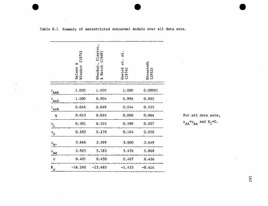
e e

Table 8.1 Summary of unrestricted autosomal models over all data sets.

e

~

~0...... +-I ...... .

..::t >-'0\ r-lt-. ell \0 ell0\ r-l0\r-l Ur-l .- - +-I +-I

~ ~ Qi 't:tI-l I-l,.c: Qi

I-l ::l ::l U r-l ...... +-I ......Qi~ ~ .,-j Qi..::t UlNN 0 o Qi +-It-. l=llt"l

r-l l=l l=lP:: QiO\ QiO\Qi .,-j .,-j Or-l +-Ir-l::C~ ~..., 0- V,l-

TAAA

1.000 1.000 LOOO 0.00001

TAaA 1.000 0.904 0.996 0.995

TaaA 0.046 0.049 0.044 0.535

q 0.013 0.016 0.006 0.064 For all data sets,

Yl0.501 0.535 0.589 0.107 ~AA=~Aa and K1=0.

Y2 0.182 0.178 0.164 0.050

~A-3.666 3.569 3.600 3.649

~aa 5.925 5.183 5.476 5.868

a 0.491 0.450 0.467 0.436

K -16.240 -15.483 -1.455 -0.4140

.....0\"-J

168

different estimates, particularly of the transmission probabilities

and susceptibilities. This is also the only set of data in which the

environmental hypothesis is not easily rejected, so the difference in

transmission probability estimates is not surprising.

The consistency of transmission probabilities in the other three

sets of data is noteworthy. In all cases these estimates are, approxi-

mately, TAM = T = 1 and T = O. In addition, the models are suchAaA aaA

that there are only two kinds of individuals: those susceptible to

affective illness and those not susceptible. Therefore, the transmis-

sion probabilities may be interpreted as follows: individuals who have

susceptible parents are susceptible, and individuals who have parents

who are not susceptible are themselves not susceptible. It appears

that there is a form of vertical transmission, though it does not con-

form to Mendelian segregation at a single locus.

Several two locus models were examined in the hope that a

slightly more complex model might prove to have a significantly better

fit. This. proved futile, perhaps not surprisingly in view of the

resounding rejection of the single locus models. None of the two gene

models resulted in a likelihood sufficiently larger than that of

the single gene models to even warrant formally testing the Mendelian

hypothesis. All of the models examined were of one autosomal and one

X-linked gene, and have been previously suggested to explain the trans-

mission of manic depressive illness. There are, of course, many

other possible two locus models. Other reasonable models might

include those with two autosomal or two X-linked genes, or models

involving more complicated types of interaction between the two loci.

However, there is absolutely nothing in any of the sets of data to

169

suggest that a different two locus model might be adequate to explain

the transmission of this disease. It is unlikely that an exhaustive

search of the possible two locus models would result in one that fit

the data well.

The results of segregation and linkage analysis of the single

large family (Chapter VII) are quite different from the results in

a group of families. In this family, both the X-linked and the

autosomal Mendelian models fit very well. However, the environmental

model also fits, although less well. An attempt was made to look

for other local maxima, and each set of initial estimates led to a

different set of maximum likelihood estimates, all with nearly equal

likelihoods. The likelihood surface must be extremely flat for such

a wide variety of parameter values to result in very similar likeli­

hoods. As a result, nothing definite can be concluded from the

segregation analysis on this family.

Linkage analysis provides some support for the hypothesis that

there exists a gene for manic depressive illness that is closely

linked to that Xg locus. There is no suggestion of linkage with

colorblindness, which is compatible with the large distance between

colorblindness and Xg. The maximum lod score for xg is far too small

for linkage to be accepted, but the suggestion of a possible linkage

provides incentive to collect more data on families of this kind.

The results of Chapters III through VI indicate that an X-linked gene

is not the most common mechanism for transmission of manic depressive

illness, but is is possible that there are rare families in which

the disease is caused by an X-linked gene.

170

The method of analysis used in this dissertation alleviates

some of the difficulties encountered in analyzing the genetics of

manic depressive illness. All the information present in the

families is used, since there is no need to break the families into

groups of parents and their children, or to analyze only first degree

relatives of probands. The extremely variable age of onset is taken

into account in a manner specifically tailored for a lognormal

distribution, which is well approximated by the empiric distribution

observed among affectively ill individuals. Ascertainment of

families through a proband is allowed for, and the possibility

that the probability of a bipolar person being a proband varies

with age of onset is considered. Finally, the method allows the

rigorous testing of the hypothesis of a major gene against a general

alternative.

The increased power of this method over previously applied

methods is obvious. It was possible to reject an autosomal

dominant, an X-linked dominant, and three two-locus models as the

mode of inheritance of manic depressive illness. All of these models

had been suggested and had received some support from various

investigators, but none could be either confidently rejected or

strongly supported by previous methods of analysis.

It must be admitted that the models examined were quite simple,

and it is perhaps not surprising that they are untenable explana­

tions for a disease as complex as manic depressive illness. Several

things can be done within the structure of the method to generalize

the model somewhat. It would be possible to allow sex differences

171

in the age of onset distribution parameters or the susceptibilities,

or both. Similarly, it would be possible to allow the suscepti­

bilities and/or the variance of age of onset to depend on genotype

In particular, it is possible that allowing sex differences in

susceptibilities and the means of age of onset within the framework

of an autosomal model could account for the observed excess of ill

women and the segregation ratios in parents, sibs and children of

probands that look like something between an X-linked and an

autosomal gene. Further analyses of this kind are left for future

projects. However, it is unlikely (though possible) that such rela­

tively minor generalizations could result in an acceptable model,

given the consistent and easy rejection of the simpler model.

An assumption underlying the genetic analysis is that there is

no non-genetic correlation in phenotype among family members. This

assumption is almost certainly violated for mental illnesses.

It is likely that there is a positive correlation among sibs, and

between parents and offspring. The method has been found to be

quite robust against sibling environmental correlation (Go et. al.

1977), at least for quantitative traits in nuclear families.

Obviously, any violation of this assumption did not lead to the

detection of a spurious major gene in these data.

Some potential difficulties with the analysis arise with regard

to the asymptotic maximum likelihood theory. If the sample size

is large enough the likelihood surface will have just one maximum

and the peak will be fairly sharp (eg., Kendall and Stuart 1973).

This is not the case with these data. The likelihood surface is

172

apparently quite flat, at least over a fairly wide region under the

Mendelian hypothesis. Several different sets of initial estimates

led to different sets of final estimates that had nearly equal

likelihoods. This effect seemed to be most pronounced in the Lava

family (see Chapter VII) and in the data of Helzer and Winokur

(1974) (Chapter III). There may well be more than one distinct

local maximum, and the standard errors of the estimates are almost

certainly large. It is also possible that twice the absolute

difference in log likelihoods between a restricted and an unre­

stricted model does not have the asymptotic X2 distribution.

If the results of the analysis were borderline these

difficulties might be troublesome, but given the very large

X2 values for testing the Mendelian hypothesis and the consistency

of results over all data sets, the conclusions are not suspect

for these reasons.

Many of the problems involved in the analysis of mental illnesses

remain untouched by the methods applied in this dissertation. It

is possible that any genetic mechanism remains obscurred because

clinical diagnoses do not correspond to specific genotypes. More

work needs to be done on the definition and delineation of affective

illnesses, including investigation of biochemical differences

between well and ill people.

One of the difficulties in analyzing many families as one set

of data is that genetic heterogeneity of the disease is a possibility

and may cloud a genetic mechanism that is operating in some of the

families but not others. The two locus "heterogeneity" model was

173

an attempt at detecting any clear-cut heterogeneity in the data.

Analysis of a single large family (the Lava family) should reduce

heterogeneity to a minimum since there should be no more than one

genetic mechanism operating within a family. However. this approach

leads to other problems. such as getting reliable information on

distant relatives and having a large enough sample so that the

asympotic theory holds.

Another approach is to select families to be analyzed on

the basis of some criterion of family history. such as selection

of families with two or more affectively ill people or elimination

of families with father to son transmission. Sampling corrections

for these cases were worked out in Chapter II. but their application

awaits the development of computer programs. Approximate techniques

may be necessary since the amount of computer time and storage

required is apt to become very large.

More complex genetic models might also be examined. The mixed

model of a major gene plus polygenic and environmental variation

might prove to be more reasonable than the models investigated

here. This also must wait until appropriate computer programs are

developed.

The results presented in Chapters III through VI indicate that

the relatively simple genetic models thus far proposed for manic

depressive illness cannot account for the transmission of the

disease in the majority of families. while the linkage analysis

of Chapter VII does not discount the possibility that there is an

occasional family in which an X-linked gene causes the disease.

174

Table 8.1 suggests that there is some type of vertical transmission,

though it need not be genetic. Cultural inheritance, or even a

virus might be involved. If there is a genetic mechanism involved

in the transmission of manic depressive illness in a majority of

families with the disease, it must be much more complex than a single

major gene or the interaction of genes at two loci.

BIBLIOGRAPHY

Abrams, R. and M.A. Taylor (1974). Unipolar mania: A preliminaryreport. Arch Gen Psychiat 30: 441-443.

Allen, M.G., S. Cohen, W. Pollin, S.I. Greenspan (1974). Affectiveillness in veteran twins: A diagnostic review. Am J Psychiat131:1234-1239.

Amark, C. (1951). A study in alcoholism. Acta Psychiat et NeurolScand Supp! 70.

American Psychiatric Association (1968). Diagnostic and StatisticalManual of Mental Disorders, 2nd edition.

August, J. (1961). A clinical analysis of the effects of Tofranil indepression. Psychopharmacologica 2:381-407.

Angst, J. (1966). Zur Atiologie und Nosologie endogener DepressiverPsychosen. Springer-Verlag, Berlin. Cited in C. PerrisActa Psychiat Scand Suppl.203:45-52 (1968).

Baker, M., J. Dorzab, G. Winokur, R. Cadoret (1972). Depressiveillness: Evidence favoring polygenic inheritance based on ananalysis of ancestral cases. Arch Gen Psychiat 27:320-327.

Batschelet, E. (1962). Spurious correlation of the age of onset, withspecial reference to asthma bronchial and atopic rhinitis.Biometrische Zeitschrift 4:111-120.

Batschelet, E. (1963). Testing hypotheses and estimating parametersin human genetics if the age of onset is random. Biometrika50:265-279.

Baldwin, J.A. (1971). Five year incidence of reported psychiatricdisorder. In International Psychiatry Clinics, ed. J.A. Baldwin,Little, Brown & Co., Boston.

Book, J.A. (1953). A genetic and neuropsychiatric investigation of anorth Swedish population. Acta Genet et Statist Med 4:1-100.

Bratfos, o. and J.O. Haug (1968). The course of manic depressivepsychosis. Acta Psychiat Scan~ 44:89-111.

176

Brodie, H.K.H. and M.J. Leff (1971). Bipolar depression--Acomparative study of patient characteristics. Am J Psychiat127:1086-1090.

Brown, R.J., R.C. Elston, W.S. Pollitzer, A. Prange, I. Wilson(1973). Sex ratio in relatives of patients with affectivedisorder. Biol Psychiat 6:307-309.

Bunney, W.E., E.S. Gershon, D.L. Murphy, F.F. Goodwin (1972). Psycho­biological and pharmacological studies of manic depressiveillness. J Psychiat Res 9:207-226.

Burch, P.R.J. (1964). Manic depressive psychosis: Some newetiological considerations. Brit J Psychiat 110:808-817.

Cadoret, R.J. and G. Winokur (1975). X-linkage in manic depressiveillness. Ann Rev Med 26:21-25.

Cadoret, R.J., G. Winokur, P. Clayton (1970). Family history studies:VII. Manic depressive disease vs. depressive disease. Brit JPsychiat 116:625-635.

Cadoret, R.J., G. Winokur, P. Clayton (1971). Family history studies:VI. Depressive disease types. Compr Psychiat 12:148-155.

Carter, T.C. and D.S. Falconer (1951). Stocks for detecting linkagein the mouse, and theory of their design. J Genet 50:307-323.

Clancy, J., M. Tsuang, B. Norton, G. Winokur (1974). The Iowa 500:A comprehensive study of mania, depression and schizophrenia.J Iowa Med Soc 64:394-398.

Clayton, P., F.N. Pitts, G. Winokur (1965). Affective disorder:IV. Mania. Compr Psychiat 6:313-322.

Clayton, P., L. Rodin, G. Winokur (1968). Family history studies:III. Schizoaffective disorder, clinical and genetic factorsincluding a one to two year followup. Compr Psychiat 9:31-49.

Cook, P.L., J. Noades, D.A. Hopkinson, E.B. Robson (1972). Demonstra­tion of sex difference in recombination fraction in the looselinkage Rh and PGM1 • Ann Hum Gen 35:239-242.

Crowe, R.R. and P.E. Smouse (1976). Age dependent penetrance inmanic-depressive illness, and its implications. In press.

Defrise-Gussenhoven, E. (1962). Hypotheses de dimerie et de non­pen6trance. Acta Genet Basel 12:65-96.

177

Denniston, C. (1969). A note on the detection of linkage of apossible X-linked locus to a known X-linked locus. Appendixto K.N. McRae, I.A. Uchida, M. Lewis, Sex linked congenitaldeafness. Am J Hum Genet 21:415-422.

Dunner, D.L. and R.R. Fieve (1975). Psychiatric illness in fathersof men with primary affective illness. Arch Gen Pschiat32:1134-1137.

Edwards, J.H. (1960). The simulation of mende1ism. Acta Genet10:63-70.

Edwards, J.H. (1971). The analysis of X-linkage. Ann Hum Genet34:229-249.

E1andt-Johnson, R.C. (1973). Age at onset distribution in chronicdiseases. A life table approach to analyses of family data.J Chronic Dis 26:529-545.

Elston, R.C. (1973). Ascertainment and age of onset in pedigreeanalysis. Human Heredity 23:105-112.

Elston, R.C., K.K. Namboodiri, M.A. Spence, J.D. Rainer (1977). Agenetic study of schizophrenia pedigrees. II. One-locushypotheses. Neuropsychobio10gy, in press.

Elston, R.C. and J. Stewart (1971). A model for the genetic analysisof pedigree data. Human Heredity 21:523-542.

Elston, R.C. and K.C. Yelverton (1975). General models forsegregation analyses. Am J Hum Genet 27:31-45

Feighner, J.P., E. Robbins, S.B. Guze, R.A. Woodruff, G. Winokur,R. Munoz (1972). Diagnostic criteria for use in psychiatricresearch. Arch Gen Psychiat 26:57-63.

Fieve, R.R., J. Mende1wicz, F.L. F1eiss (1973). Manic depressiveillness: Linkage with Xg blood group. Am J Psychiat130:1355-1359.

Finney, D.J. (1940). The detection of linkage I. Ann Eugen10:171-214.

Finney, D.J. (1941). The detection of linkage II. Ann Eugen 11:10-30.

Finney, D.J. (1941). The detection of linkage III. Ann Eugen11J115-135.

Finney, D.J. (1942). The detection of linkage IV. Ann Eugen11:224-232.

Finney, D.J. (1942). The detection of linkage VI. Ann Eugen11:233-244.

178

Finney, D.J. (1943). The Detection of linkage VII. AnnEugen12:31-43.

Fisher, R.A. (1943).abnormalities.

Fisher, R.A. (1935).abnormalities.

The detection of linkage with "dominant"Ann Eugen 6:187-201.

The detection of linkage with recessiveAnn Eugen 6:339-350.

Fraser, G.R. (1968). Some complications of the use of the threegeneration method in the estimation of linkage relationshipson the X-chromosome in man. Ann Hum Genet 32:65-79.

Fraser, G.R. and O. Mayo (1968). A comparison of the two-generationand three-generation methods of estimating linkage values of theX-chromosome in man with special reference to the loci determin­ing the Xg blood group and G6PD deficiency. Am J Hum Genet20:534-548.

Gershon, E.S., W.E. Bunney, J.F. Leckman, M. Van Eerdewegh, B.A.DeBauche, (1976). The inheritance of affective disorders: Areview of data and of hypotheses. Behaviour Genetics 6:227-261.

Gershon, E.S., D.L. Dunner, F.K. Goodwin (1971).affective disorders: Genetic contributions.25:1-15.

Toward a biology ofArch Gen Psychial

Gershon, E.S., and W.E. Bunney (1976). The question of X-linkage inmanic-depressive illness. J Psychiat Res 13:99-117.

Gershon, E.S., D.L. Dunner, L. Sturt, F.F. Goodwin (1973). Assorta­tive mating in the affective disorders. BioI Psychiat 7:63-74.

Gershon, E.S. and S. Matthysse (1977). X-linkage: Ascertainmentthrough doubly ill probands. J Psychiat Res, in press.

Go, R.C.P., R.C. Elston, and E.B. Kaplan (1977).robustness of pedigree segregation analysis.in press.

Efficiency andAm J Hum Genet,

Goetzl, U., R. Green, P. Whybrow, R. Jackson (1974). X-linkagerevisited: A further family study of manic depressive illness.Arch Gen Psychiat 31:665-672.

Haldane, J.B.S. and C.A.B. Smith (1947). A new estimate of thelinkage between the genes for colorblindness and hemophiliain man. Ann Eugen 14:10-31.

Hartl, D.L. and T. Maruyama (1968). Phenogram enumeration: Thenumber of regular phenotype-genotype correspondences ingenetic systems. J Theoret BioI 20:129-163.

179

Harvald. B. and M. Hauge (1965). Hereditary factors elucidated bytwin studies. in Genetics and the Epidemiology of ChronicDiseases.

Helgason. T. (1964). Epidemiology of·mental disorders in Iceland.Acta Psychiat Scand Suppl. 1973.

Helzer. J.E. (1975). Bipolar affective disorder in black and whitemen. Arch Gen Psychiat 32:1140-1143.

Helzer. J. and G. Winokur (1974). Family interview study of malemanic depressives. Arch Gen Psychiat 31:73-77.

Hoffman. H. (1921). Die Nichkommenschaft be! endogen Psychosen.Berlin. cited in E. Slater. Proc Roy Soc Med 29:981-990. 1935.

Hopkinson. G. and P. Ley (1969). A genetic study of affectivedisorder. Brit J. Psychiat 115:917-922.

Jackson, C.E .• W.E. Symon, J.D. Mann (1964). X chromosome mapping ofgenes for red-green co1orb1indness and Xg. Am J Hum Genet16:403-409.

Janowsky. D.S .• J.M. Davis. M. Khaled E1-Yousef. H.J. Sekerke (1972).A cholinergic-adrenergic hypothesis of mania and depression.Lancet 2:632-635.

Kallman. F.J. (1950). The genetics of psychoses. Congres Inter­nationale de Psychiatrie. vol. 6, Hermann & C1e • Paris.

Kallman. F.J. (1954). Genetic principles in manic depressivepsychosis. in Depression. ed. Hoch. P.H. and J. Zubin.Grune and Stratton. New York.

Kaplan. E.B. and R.C. Elston (1973).likelihood estimation (MAXLIK).Mimeo Series No. 823, UNC.

A subroutine for maximumInstitute of Statistics

Kendall. M.G. and A. Stuart (1973). The Advanced Theory of Statisticsvol. 2. Hafner Publishing Co .• New York.

Kraeplin. E. (1907). Lehrbuch der Psychiatrie. translated andabstracted from the 7th German edition by A.R. Diefendorf asClinical Psychiatry. MacMillian & Co. Ltd •• London.

Kraeplin, E. (1917). Lectures in Clinical Psychiatry. 3rd

Englished .• trans. and ed. by T. Johnstone. William Wood & Co •• NewYork.

Kringlen. E. (1967). Heredity and Environment in the FunctionalPsychoses. William Heinemann Medical Books. Ltd. London.

180

Kosambi, D.D. (1944). The estimation of map distances fromrecombination values. Ann Eugen 12:172-175.

Lange, K. and R.C. Elston (1975). Extensions to pedigree analysisI. Likelihood calculations for simple and complex pedigrees.Hum Hered. 25:95-105.

Lange, K., B.M. Page, R.C. Elston (1975). Age trends in humanchiasma frequencies and recombination fractions, I. Chiasmafrequencies. Am J Hum Genet 27:410-418.

Levitan, M. and A. Montagu (1971). Textbook of Human Genetics,Oxford University Press, New York.

Luxenburger, H. (1932). Nervenarzt 5:505, cited in A. Stenstedt,Acta Psychiat et Neuro1 Scand Suppl. 79 (1952).

MacLean, C.J., N.E. Morton and R. Lew (1975). Analysis of familyresemblence IV. Operational characteristics of segregationanalysis. Am J Hum Genet 27:365-384.

Maynard-Smith, S., L.S. Penrose, C.A.B. Smith (1961). MathematicalTables for Research Workers in Human Genetics, Churchill, London.

Mayo, O. (1970). The use of linkage in genetic counselling. HumanHeredity 20:473-485.

Mendlewicz, J., R.R. Feive, J.D. Rainer, M. Cataldo (1973). Affectivedisorder on paternal and maternal sides: Observations inbipolar patients with and without a family history. Brit JPsychiat 122:31-34.

Mend1ewicz, J., R.R. Fieve, J.D. Rainer, J.L. F1eiss (1972). Manicdepressive illness: A comparitive study of patients with andwithout a family history. Brit J Psychiat 120:523-530.

Mendlewicz, J., R.R. Fieve, F. Sta1lon (1973). Relationship betweenthe effectiveness of lithium therapy and family history. Am JPsychiat 130:1011-1013.

Mend1ewicz, J., and J.L. Fleiss (1974). Linkage studies with X­chromosome markers in bipolar (manic depressive) and unipolar(depressive) illnesses. BioI Psychiat 9:261-294.

Mendlewicz, J., J.L. F1eiss, M. Cataldo, J.D. Rainer (1975). Accuracyof the family history method in affective illness. Arch GenPsychia~ 32:309-314.

Mendlewicz, J., J.L. Fleiss, R.R. Fieve (1972). Evidence for X­linkage in the transmission of manic depressive illness.JAmMed Assoc 222:1624-1627.

181

Mendlewicz, J. and J.D. Rainer (1974). Morbidity risk and genetictransmission in manic depressive illness. Am J Hum Genet26: 692-701.

Mitsuda, H. (1965). The concept of "atypical psychoses" from theaspect of clinical genetics. Acta Psychiat Scand41:372-377 .

Morrison, J.R. (1975). The family histories of manic depressivepatients with and without alcoholism. J Nerv Ment Dis160:227-229.

Morrison, J.R., J. Clancy, R. Crowe, G. Winokur (1972). The Iowa500: I. Diagnostic validity in mania, depression andschizophrenia. Arch Gen Psychiat 27:457-461.

Morton, N.E. (1955). Sequential tests for the detection of linkage.Am J Hum Genet 7:277-318.

Morton, N.E. (1956). The detection and estimation of linkage betweenthe genes for elliptocytosis and the Rh blood type. Am J HumGenet 8:80-96.

Morton, N.E. (1957). Further scoring types in sequential tests, witha critical review of autosomal and partial sex linkage in man.Am J Hum Genet 9:55-75.

Morton, N.E. (1969). Segregation analyses. In Computer Applicationsin Genetics, ed. N.E. Morton. University of Hawaii Press,Honolulu, Hawaii, pp. 129-137.

Morton, N.E., S. Yee, R. Lew (1971). Complex segregation analysis.Am J Hum Genetics 23:602-611.

Morton, N.E. and C.J. MacLean (1974). Analysis of family resemb1enceIII. Complex segregation of quant1tative traits. Am J HumGenet 26:489-503.

Munro, A. (1965). Depressive illness in twins. Acta Psychiat Scand41:111-116.

O'Brien, W.M., C.C. Li, F.H. Taylor (1965). Penetrance and thedistribution of sib-pair types, exemplified by taste abilityand rheumatoid arthritis. J. Chron Dis 18:675-680.

Ott, J. (1974).pedigrees.

Estimation of the recombination fraction in humanAm J Hum Genet 26:588-597.

Pare, C.M.B.', L. Rees, M.J. Sainsbury (1962). Differentiation oftwo genetically specific types of depression by the responseto antidepressants. Lancet 2:1340-1343.

182

Pare, C.M.B. and J.W. Mack (1971). Differentiation of twogenetically specific types of depression by the response to .antidepressant drugs. J Med Genet 8:306-309.

Penrose, L.S. (1935). The detection of autosomal linkage in datawhich consists of pairs of brothers and sisters of unspecifiedparentage. Ann Eugen 6:133-138.

Penrose, L.S. (1946). A further note on the sib-pair linkage method.Ann Eugen 13:25-29.

Penrose, L.S. (1953). The general purpose sib-pair linkage test.Ann Hum Genet 18:120-124.

Perris, C. (1968a). Genetic transmission of depressive psychoses.Acta Psychiat Scand Supp1. 203:45-52.

Perris, C. (1968b). The course of depressive psychoses. ActaPsychiat Scand 44:238-248.

Perris, C. (1969). The separation of bipolar from unipolar recurrentdepressive psychoses. Behavioral Neuropsychiatry 1:17-24.

Perris, C. (1971). Abnormality on paternal and maternal sides:Observations in unipolar and bipolar depressive psychoses.Brit J Psychiat 118:207-210.

Perris, C. (1974). A study of cycloid psychoses. Acta PsychiatScand Supp1. 253.

Pitts, F.N. and G. Winokur (1964). Affective disorder: III. Diag­nostic correlates and incidence of suicide. J Nerv Ment Dis139:176-181.

Pitts, F.M. and G. Winokur (1966). Affective disorder: VII.Alcoholism and affective disorder. J Psychiat Res 4:37-50.

Porter, I.H., J. Schulze, V.A. McKusick (1962). Genetical linkagebetween the loci for G6PD deficiency and co1orb1indness inAmerican Negroes. Ann Hum Genet. 26:107-118.

Price, J. (1968). The genetics of depressive behavior. in RecentDevelopments in Affective Disorders, Coppen, H. and A. Walk,eds. Headley Brothers Ltd., London.

Reich, T.P. Clayton, G. Winokur (1969). Family history studies:V. The genetics of mania. Am J Psychiat 125:1358-1369.

Renwick, J.H. (1961). Elucidation of gene order. In Recent Advancesin Human Genetics, L.S. Penrose and H.L. Brown, eds. Little,Brown & Co. Boston.

183

Renwick, J.H. (1969). Progress in mapping human autosomes. Brit MedBull 25:65-73.

Renwick, J.H. (1971). The mapping of human chromosomes. Ann RevGenet 5:81-120.

Renwick, J.H. and D.R. Bolling (1971). An analysis procedure illus­trated on a triple linkage of use for prenatal diagnosis ofmyotonic dystrophy. J Med Gen 8:399-406.

Renwick, J.H. and J. Schulze (1964). An analysis of some data onthe linkage between Xg and colorblindness in man. Am J HumGenet 16:410-418.

Rosanoff, A.J., L.M. Handy, l.R. Plesset (1935). The etiology ofmanic depressive syndromes with special reference to theiroccurence in twins. Am J Psychiat 91:725-762.

Rosenthal, D. (1970). Genetic Theory and Abnormal Behavior, McGraw­Hill Book Co., New York.

Rudin, E. (1923). Zeitschr. f. d. ges. Neural. u. Psychiat. 8:459.Cited in E. Slater Proc Roy Soc Med 29:981-990.

Slater, E. (1935). The inheritance of manic depressive insanity.Proc Roy Soc Med 29:981-990.

Slater, E. (1938). Z ges Neural Psychiat 163:1-47. Cited inT. Helgason, Acta Psychiat Scand Supp1 173 (1964).

Slater, E. (1966). Expectation of abnormality on paternal andmaternal sides: A computational model. J Med Genet 3:159-161.

Slater, E. J. Maxwell, J.S. Price (1971). Distribution of ancestralsecondary cases in bipolar affective disorders. Brit J Psychiat118:215-218.

Smith, C. (1971). Discriminating between different modes of inheri­tance in genetic disease. C1in Genet 2:303-314.

Smith, C.A.B. (1953). The separation of the sexes of parents in thedetection of linkage in man. Ann Hum Genet 18:278-301.

Smith, C.A.B. (1953b). The detection of linkage in human genetics.J Roy Statist Soc (B2. 15: 153-192.

Smith, C.A.B. (1959).linkage analysis.

Some comments on statistical methods used inAm J Hum Genet 11:289-304.

Smith, C.A.B. (1961). Statistical methods and theory. In RecentAdvances in Human Genetics, L.S. Penrose and H.L. Brown, eds.Little, Brown & Co., Boston.

184

Smith, C.A.B. (1963). Testing for heterogeneity of recombinationvalues in human genetics. Ann Hum Genet 27:175-182,.

Smith, C.A.B. (1968). Linkage scores in two- and three-generationfamilies. Ann Hum Genet 32:127-150.

Smith, C.A.B. (1969). Further linkage scores and corrections intwo- and three-generation families. Ann Hum Genet 33:207-223.

Spence, M.A., R.C. Elston, K.K. Namboodiri, and J.D. Rainer (1977).A genetic study of schizophrenia pedigrees. I. Demographicstudies: sample description, age of onset, ascertainment andclassification. Neuropsychobiology 2:328-340.

Steinberg, A.G. and N.E. Morton (1956). Sequential test for linkagebetween cystic fibrosis of the pancreas and the MNS locus.Am J Hum Genet 8:177-189.

Stenstedt, A. (1952). A study in manic depressive psychosis. ActaPsychiat et Neuro1 Scand Supp1. 79.

Stenstedt, A. (1959). Involutional melancholia. Acta Psychiat etNeuro1 Scand Supp1. 127.

Stromgren, E. (1965). Schizophreniform psychoses. Acta PsychiatScand 41:483-489.

Tanna, V.L. and G. Winokur (1968). A study of association and linkageof ABO blood types and primary affective disorder. Brit JPsychiat 114:1175-1181.

e-

Taylor, M. and R. Abrams (1973). Manic states:early and late onset affective disorders.28:656-8.

A genetic study ofArch Gen Psychiat

Tienari, P. (1963). Psychiatric illness in identical twins. ActaPsychiat Scand Supp1. 171.

Thompson, G. (1977). The effect of a selected locus on linkedneutral loci. Genetics 85:753-788.

Tomasson, H. (1938). Further investigations on manic depressivepsychosis. Acta Psychiat et Neuro1 Scand 13:517-523.

Tranke11, A. (1955). Aspects of genetics in psychology. Am J HumGenet 7:264-276.

Tranke11, A. (1956). Penetrance calculus in population genetics.Am J Hum Genet 8:44-48.

Vogt, R. (1910). Tiddsskrift for den norski 1aegeforening 30:417.Cited in A. Stenstedt Acta Psychiat et Neuro1 Scand Supp1 79(1952).

185

Von Grieff, H., P.R. McHugh, P.E. Stokes (1975). The familialhistory in 16 males with bipolar manic depressive illness.In Genetic Research in Psychiatry, eds. R.R. Fieve, D. Rosenthaland H. Brill. The Johns Hopkins University Press, Baltimore,pp. 219-232.

Weitkamp, L.R. (1972). Human autosomal linkage maps. In Proceedingsof the 4th International Congress of Human Genetics,J. deGrouchy, F.J.G. Ebling, and J.W. Henderson, eds. ExcerptaMedica, Amsterdam, pp. 445-460.

Wilson, S.R. (1971). Fitting model of incomplete penetrance tofamily data. Ann Hum Gen 35:99-108.

Wilson, S.R. (1974). Simulation of Mendelism by a non-genetic Markovchain model. Ann Hum Genet 38:225-229.

Winokur, G. (1970). Genetic findings and metholological considera­tions in manic depressive disease. Brit J Psychiat 117:267-274.

Winokur, G. (1971). The genetics of manic depressive illness. InDepression in the 70's R.R. Fieve, ed. Excerpta Medica, Amsterdam.pp. 47-53.

Winokur, G. (1975). The Iowa 500:depressive illness (bipolar).

Heterogeneity and course in manicCompr Psychiat 16:125-131.

Winokur. G., R. Cadoret, J. DorzaL, M~ Baker (1971). Depressivedisease: A genetic study. Arch Gen Psychiat 24:135-144.

Winokur, G. and P. Clayton (1967a). Family history studies: II. Sexdifferences and alcoholism in primary affective illness.Brit J. Psychiat 113:973-979.

Winokur, G. and P. Clayton (1967b).types of affective disorders.Psychiatry, vol. 9. J. Wortis,

Family history studies: I. TwoIn Recent Advances in Biologicaled. Plenum Press, New York.

Winokur, G., P. Clayton, T. Reich (1969). Manic Depressive Illness.The C.V. Mosley Co., St. Louis

Winokur, G., J. Morrison, J. Clancy, R. Crowe (1972).II. A blind family history comparison of mania,schizophrenia. Arch Gen Psychiat 27:462-464.

The Iowa 500:depression and

Winokur, G., and F.N. Pitts (1964).reactive depression an entity?

Affective disorder: I. IsJ Nerv Ment Dis 138:541-547.

Winokur, G., and F.N. Pitts (1965). Affective disorder: II. Afamily study of prevalences, sex differences and possiblegenetic factors. J Psychiat Res 3:113-123.

186

Winokur, G., and T. Reich (1970). Two genetic factors in manicdepressive disease. Compr Psychiat 11:93-99.

Winokur, G., J. Rimmer, T. Reich (1971). Alcoholism: IV. Is theremore than one type of alcoholism? Brit J Psychiat 118:125-131.

Winokur, G., and S. Ruangtrakoo1 (1966). Genetic vs. nongeneticaffective disorder. Am J Psychiat 123:703-705

Winokur, G., and V.L. Tanna (1969). Possible role of X-linkeddominant factor in manic depressive disease. Dis Nerv Sys30:89-94.

Woodruff, R., F.N. Pitts, G. Winokur (1964). Affective disorder:II. A comparison of patients with endogenous depressions withand without a family history of affective disorder. J NervMent Dis 139:49-52.

Yelverton, K.C., K.K. Naboodiri, R.C. Elston (1975). GeneralSegregation Analysis Package Writeup (GENSEG), unpublished.