The finite sample performance of estimators for mediation analysis

under sequential conditional independence

Martin Huber*, Michael Lechner**, and Giovanni Mellace+

*University of Fribourg, **University of St. Gallen, +University of Southern Denmark

Abstract: Using a comprehensive simulation study based on empirical data, this paper investigates

the finite sample properties of different classes of parametric and semi-parametric estimators of (natural)

direct and indirect causal effects used in mediation analysis under sequential conditional independence

assumptions. The estimators are based on regression, inverse probability weighting, and combinations

thereof. Our simulation design uses a large population of Swiss jobseekers and considers variations of

several features of the data generating process and the implementation of the estimators that are of

practical relevance. We find that no estimator performs uniformly best (in terms of root mean squared

error) in all simulations. Overall, so-called ‘g-computation’ dominates. However, differences between

estimators are often (but not always) minor in the various setups and the relative performance of the

methods often (but not always) varies with the features of the data generating process.

Keywords: Causal mechanisms, direct effects, indirect effects, simulation, empirical Monte Carlo Study,

causal channels, mediation analysis, causal pathways.

JEL classification: C21.

We have benefited from comments and advice by Kosuke Imai, Eric Tchetgen Tchetgen, Mark van der Laan,

Teppei Yamamoto, Wen Zheng, an associate editor, and three anonymous referees. Addresses for correspondence:

Martin Huber (martin.huber@unifr.ch), Department of Economics, University of Fribourg, Bd. de Perolles 90, CH-

1700 Fribourg; Michael Lechner (michael.lechner@unisg.ch), Swiss Institute for Empirical Economic Research, Uni-

versity of St. Gallen, Varnbuelstrasse 14, CH-9000 St. Gallen; Giovanni Mellace (giome@sam.sdu.dk), Department

of Business and Economics, University of Southern Denmark, Campusvej 55, DK-5230 Odense M. Michael Lechner

and Giovanni Mellace gratefully acknowledge financial support from the Swiss National Science Foundation grant

number 100018 137769. Michael Lechner is also a Research Fellow of CEPR and PSI, London, CES-Ifo, Munich,

IAB, Nuremberg, and IZA, Bonn. The usual disclaimer applies.

1 Introduction

A vast empirical literature in statistical and social sciences is concerned with the estimation of

causal effects, both in randomized experiments and in observational studies. However, in many

studies not only the causal effect per se appears interesting, but also the causal mechanisms

through which it operates. Or, as Gelman and Imbens (2013) argue, very often not only the

‘effects of causes’ appear relevant, but also the ‘causes of effects’. For example, when assessing

the employment or earnings effects of an active labor market program, policy makers might want

to know to which extent the total impact comes from increased search effort, human capital, or

other mediators that are themselves affected by the program. It is therefore no surprise that the

analysis of the causal mechanisms through which an initial treatment variable affects an outcome

of interest, also referred to as mediation analysis, has become more relevant in empirical work

across disciplines such as economics, epidemiology, political science, and statistics. Identification

requires controlling for the potential endogeneity of the treatment and the intermediate variables

through which the causal mechanisms operate (i.e. through which the treatment ultimately affects

the outcome of interest), the so-called mediators. Under particular assumptions, the (total) causal

effect may then be disentangled in an indirect component related to one or several mediators and

a direct effect, which includes all remaining causal channels not covered by the mediators of

interest.

The majority of studies in mediation analysis assumes that all potential confounders jointly

affecting the treatment, the mediator, and the outcome (and thus potentially causing treatment

and/or mediator endogeneity) are observed (and are not a function of the treatment).1 This

amounts to assuming a sequential conditional independence (or ignorability) assumption

w.r.t. the mediator and the treatment. It requires (i) that the potential outcomes and the

treatment are independent given the observed covariates and (ii) that the potential outcomes

and the mediator are independent given the covariates and the treatment, see for instance Imai,

1If some confounders of the mediator are a function of the treatment, identification becomes more difficult, seefor instance the discussion in Robins (2003), Avin, Shpitser, and Pearl (2005), Albert and Nelson (2011), Imai andYamamoto (2013), and Huber (2014).

1

Keele, and Yamamoto (2010) or the closely related assumptions in Pearl (2001) and Flores

and Flores-Lagunes (2009). Under this condition, various estimators of causal mechanisms

have been proposed that differ in terms of imposed functional form assumptions. One popular

approach is to estimate direct and indirect effects by a system of linear equations characterizing

the mediator (as function of the treatment and the covariates) and the outcome (as function

of the mediator, treatment, and the covariates). Consistency of the estimator requires that

both equations are correctly specified and thus, linear, which appears ill-suited e.g. for binary

mediators/outcomes. In contrast, g-computation (suggested by Robins (1986) and considered in

the context of direct and indirect effects for instance in Zheng and van der Laan (2012)) also

allows for non-linear mediator and outcome models. It estimates the parameters of interest by

the sample analogs of the so-called mediation formula, see for instance Pearl (2001). The latter

expresses direct and indirect effects as functions of the conditional mean outcomes (given the

mediator, the treatment, and the covariates) and the conditional mediator densities (given the

treatment and the covariates), which are estimated by maximum likelihood methods. Again, if

either the conditional means or the conditional densities are incorrectly specified, g-computation

is in general inconsistent.

Several more flexible semiparametric methods have been suggested more recently. Huber

(2014) uses inverse probability weighting (henceforth IPW, see the seminal paper by Horvitz

and Thompson (1952)) by treatment propensity scores (given the mediator and the covariates or

the covariates only, respectively) to estimate causal mechnisms. Furthermore, ‘multiply robust’

estimators (the equivalent to doubly robust estimation in standard treatment effect models)

have been proposed by Tchetgen Tchetgen and Shpitser (2012) (based on the efficient influence

function) and Zheng and van der Laan (2012) (based on a targeted maximum likelihood approach).

Although results about the asymptotic behavior of most estimators are available, little is known

about their comparative performance in finite samples and their robustness to misspecification

(which is almost unavoidable in empirical applications) of model components.

The contribution of this paper is to thoroughly assess the finite sample behavior of a range of

2

common estimators of direct and indirect effects under the assumption of sequential conditional

independence.2 To this end, we apply a sophisticated simulation design that is based on a large

empirical data set, an approach also advocated in Huber, Lechner, and Wunsch (2013) and

named ‘Empirical Monte Carlo study’ (EMCS) therein. To be concise, we use linked jobseeker-

caseworker data from Switzerland, which allow disentangling the effect of treatment ‘counselling

style of caseworkers’ (rigorous vs. cooperative style) on jobseekers’ employment into a direct effect

and an indirect effect running via assignment to active labor market policies (see the companion

paper Huber, Lechner, and Mellace (2014) for an empirical evaluation). Basing the simulations

on empirical data is hopefully more closely related to real world applications than conventional

Monte Carlo designs based on completely artificial (and potentially arbitrary) data generating

processes.3 We vary several simulation parameters such as sample size, effect heterogeneity,

selection into the mediator, the share of individuals assigned to active labor market policies (the

mediator), and the type of outcome (binary and non-binary), which entails a large variety of

models considered. The estimators investigated include IPW (Huber (2014)), ‘multiply robust’

estimation (influence function-based estimation of Tchetgen Tchetgen and Shpitser (2012) and

targeted MLE of Zheng and van der Laan (2012)), estimation by a system of linear equations (see

Baron and Kenny (1986)), g-computation, parametric estimation using the ‘mediation’ package

for R by Tingley, Yamamoto, Hirose, Imai, and Keele (2014) (which is consistent under the same

assumptions as g-computation), and a further flexible parametric approach based on regressions

2While the finite sample performance of estimators of direct and indirect effects appears under-researched upto date, several simulation studies compare various parametric and semiparametric estimators of total (average)effects, see for instance Frolich (2004), Zhao (2004), Lunceford and Davidian (2004), Busso, DiNardo, and McCrary(2013, 2014), and Huber, Lechner, and Wunsch (2013). The latter two papers base the simulations (at least partly)on real world data.

3Recently such a Monte Carlo approach has been criticised by Advani and Sloczynski (2013), who comparethe performance of various estimators in the so-called LaLonde (1986) data with their performance in differentMonte Carlo designs. However, their paper suffers from several drawbacks: a) The experimental estimate in theLaLonde (1986) data is taken as the true effect. In reality, however, it is only an unbiased estimate of the trueeffect. The ordering of the estimators is therefore disturbed if some estimators are closer to the true value than theexperimental estimate (which is random). b) The LaLonde data is rather small. This implies i) a noisy estimate ofthe estimated treatment model used for the placebo simulations, and ii) that the ‘population’ to draw from is rathersmall and generated samples may not reflect the statistical concept of a ‘sample drawn from a infinite population’on which inference measures are based upon. c) The conditional independence of the treatment is most likely notvalid in the LaLonde data, given the limited number of observed covariates. However, it is by construction validin the simulated data of Advani and Sloczynski (2013). Thus, the idea on which the EMCS is based, namely thatthe selection and outcome processes in the true world and the EMCS data are very similar, is likely violated forthe selection process into treatment.

3

in the subpopulations defined by the treatment state.

Our results do not point to a uniformly best performing estimator in all simulations in terms

of the root mean squared error (RMSE). Often (but not always), the differences between par-

ticular estimators are minor and their relative performance varies with the features of the data

generating process. For instance, g-computation most frequently dominates the other methods

(followed by targeted MLE) when estimating direct effects, but several estimators perform sim-

ilarly well. With regard to the indirect effects, flexible parametric regression always dominates

in the non-binary outcome case, but only under effect homogeneity when the outcome is binary,

while IPW and influence function-based estimation are preferable under effect heterogeneity and

binary outcomes. We also investigate the performance of each method when jointly estimating

direct and indirect effects, based on the norm of the joint RMSE matrix. For the non-binary

outcome, g-computation and flexible parametric estimation dominate, for the binary outcome,

g-computation and influence-based estimation are slightly better than IPW and targeted MLE.

Overall, g-computation is the preferred method in our simulations.

The remainder of the paper is organized as follows. The next section describes the parameters

of interest and the sequential conditional independence (or ignorability) assumption required for

the consistency of the estimators. Section 3 discusses the various classes of estimators considered

in the simulations. Section 4 describes the empirical Monte Carlo design and the data it is based

upon. The main results are presented in Section 4, while the further results and descriptive

statistics are provided in the appendix. Section 5 concludes.

2 Parameters of interest and identifying assumptions

Denote by D a binary intervention or treatment and by Y the outcome variable of interest.

Mediation analysis aims at disentangling the causal effect of D on Y into a direct component

and an indirect effect operating through some mediator M , which may be discrete or continuous.

Figure 1 provides a graphical illustration of the evaluation framework considered (where arrows

4

represent causal effects from one variable to another), however, omitting any confounders. To

define the parameters of interest, we use the potential outcome framework advocated by Rubin

(1974) (among many others) and considered in the direct and indirect effects framework for

instance by Rubin (2004), Ten Have, Joffe, Lynch, Brown, Maisto, and Beck (2007), and Albert

(2008). Let M(d), Y (d,M(d)) denote the potential mediator state and the potential outcome

under treatment d ∈ {0, 1}. For each unit only one of the two potential mediator states and

outcomes, respectively, is observed, because the realized outcome and mediator values are M =

D ·M(1) + (1−D) ·M(0) and Y = D · Y (1,M(1)) + (1−D) · Y (0,M(0)).

Figure 1: Graphical illustration of the mediation framework

The (total) average causal effect is given by ∆ = E[Y (1,M(1)) − Y (0,M(0))]. Exogenously

varying the treatment but keeping the mediator fixed at its potential value for some d ∈ {0, 1}

gives the (average) direct effect:

θ(d) = E[Y (1,M(d))− Y (0,M(d))], d ∈ {0, 1}, (1)

The (average) indirect effects is obtained by exogenously shifting the mediator to its potential

values under treatment and non-treatment but keeping the treatment fixed at d:4

δ(d) = E[Y (d,M(1))− Y (d,M(0))], d ∈ {0, 1}, (2)

Note that the average causal effect is the sum of the direct and indirect effects defined upon

4Pearl (2001) refers to these parameters as natural direct and indirect effects, Robins and Greenland (1992)and Robins (2003) as total or pure direct and indirect effects, and Flores and Flores-Lagunes (2009) as net andmechanism average treatment effects, respectively.

5

opposite treatment states:

∆ = E[Y (1,M(1))− Y (0,M(0))]

= E[Y (1,M(0))− Y (0,M(0))] + E[Y (1,M(1))− Y (1,M(0))] = θ(0) + δ(1)

= E[Y (1,M(1))− Y (0,M(1))] + E[Y (0,M(1))− Y (0,M(0))] = θ(1) + δ(0). (3)

This follows from adding and subtracting E[Y (0,M(1))] after the second and E[Y (1,M(0))] after

the fourth equalities. Using the notation θ(1), θ(0) and δ(1), δ(0) points to potential effect het-

erogeneity w.r.t. the treatment, i.e., interaction effects between the treatment and the mediator.

However, any effect cannot be identified without further assumptions, because either Y (1,M(1))

or Y (0,M(0)) is observed for any individual, whereas Y (1,M(0)) and Y (0,M(1)) are never ob-

served.

A good part of the literature based identification of direct and indirect effects on a sequential

conditional independence (or ignorability) assumption of the treatment and the mediator, see for

instance Imai, Keele, and Yamamoto (2010), Tchetgen Tchetgen and Shpitser (2012), and Huber

(2014). To this end, let X denote a vector of observed covariates that potentially confound the

treatment and/or mediator effect(s) on the outcome.

Assumption 1 (conditional independence of the treatment):

{Y (d′,m),M(d)}⊥D|X = x for all d′, d ∈ {0, 1} and m,x in the support of M,X.

Assumption 1 states that conditional on X, the treatment is independent of the potential mediator

states and the potential outcomes, implying that there are no unobserved confounders jointly

affecting the treatment on the one hand and the mediator and/or the outcome on the other hand

given X. This is referred to as conditional independence, selection on observables, or exogeneity

in the treatment evaluation literature, see for instance Imbens (2004).

Assumption 2 (conditional independence of the mediator):

Y (d′,m)⊥M |D = d,X = x for all d′, d ∈ {0, 1} and m,x in the support of M,X.

Assumption 2 states that conditional on D and X, the mediator is independent of the potential

6

outcomes. This implies that there exist no unobserved confounders jointly causing the mediator

and the outcome given the treatment and the covariates. Assumption 2 would for instance be

violated if unobserved pre-treatment variables affected both M and Y directly, i.e., not only

through D and X.

Assumption 3 (common support):

Pr(D = d|M = m,X = x) > 0 for all d ∈ {0, 1} and m,x in the support of M,X.

Assumption 3 is a common support restriction. The conditional probability to be treated given

M,X, henceforth referred to as propensity score, must be larger than zero in either treatment

state. This implies that Pr(D = d|X = x) > 0 must hold, too. By Bayes’ theorem, Assumption 3

also entails Pr(M = m|D = d,X = x) > 0 or, in the case of a continuous M , that the conditional

density of M given D,X is larger than zero: fM |D,X(m, d, x) > 0. In other words, conditional

on X, the mediator state must not be deterministically affected by the treatment, otherwise

comparable units in terms of mediator values across treatment states would not exist.

Under these assumptions, the direct and indirect effects are identified by the so-called me-

diation formulae, see for instance Pearl (2001) and Imai, Keele, and Yamamoto (2010), which

represent the direct and indirect effects as functions of the conditional mean of Y given D,M,X

and the conditional density of M given D,X:

θ(d) = EX

[EM |D=d,X=x [E[Y |D = 1,M = m,X = x]− E[Y |D = 0,M = m,X = x]|D = d,X = x]

],

δ(d) = EX

[EM |D=1,X=x [E[Y |D = d,M = m,X = x]|D = 1, X = x]

](4)

− EX

[EM |D=0,X=x [E[Y |D = d,M = m,X = x]|D = 0, X = x]

]. (5)

Huber (2014) shows that the parameters of interest may alternatively be expressed as functions of

the treatment propensity scores Pr(D = 1|M,X) and Pr(D = d|X), which is useful for estimation

7

based on inverse probability weighting (IPW).

θ(d) = E

[(Y D

Pr(D = 1|M,X)− Y (1−D)

1− Pr(D = 1|M,X)

)Pr(D = d|M,X)

Pr(D = d|X)

], (6)

δ(d) = E

[Y I{D = d}

Pr(D = d|M,X)

(Pr(D = 1|M,X)

Pr(D = 1|X)− 1− Pr(D = 1|M,X)

1− Pr(D = 1|X)

)]. (7)

Note that the simulations focus on the estimation of θ(0) and δ(1), while θ(1) and δ(0) are not

considered. As the estimation problems are symmetric, we would, however, expect that the overall

performance in estimating either θ(0), δ(1) or θ(1), δ(0) is similar within a particular econometric

method.

Albeit not required for non-parametric identification, a subset of parametric estimators con-

sidered below is only consistent if average treatment-mediator interaction effects on the outcome

are ruled out. This implies that average direct effects are homogeneous in the value of the medi-

ator, as formally stated in Assumption 4:

Assumption 4 (Homogeneity of average direct effects in the mediator):

E[Y (1,m)|X = x]−E[Y (0,m)|X = x] = E[Y (1,m′)|X = x]−E[Y (0,m′)|X = x] for all m,m′, x

in the support of M,X.

It follows that θ(1) = θ(0) = θ, because the direct effects are identical under M(1) and M(0),

and δ(1) = δ(0) = δ, because δ = ∆− θ.

3 Estimators

3.1 Overview

This section introduces the parametric and semiparametric estimators of direct effects investi-

gated in the simulations. The parametric methods include estimation by a system of linear equa-

tions (see Baron and Kenny (1986)), a more flexible parametric approach based on regressions

within each treatment state, g-computation (suggested by Robins (1986), considered in the con-

8

text of direct/indirect effects for instance by Zheng and van der Laan (2012)), and estimation

based on simulating potential mediators and outcomes using the ‘mediation’ package for R by

Tingley, Yamamoto, Hirose, Imai, and Keele (2014). Concerning semiparametric estimation, we

consider inverse probability weighting (Huber (2014)), and ‘multiply robust’ estimation based on

the efficient influence function (Tchetgen Tchetgen and Shpitser (2012) and targeted maximum

likelihood Zheng and van der Laan (2012)) for assessing direct and indirect effects.

3.2 Parametric methods

3.2.1 OLS estimation of a system of linear equations

Following Baron and Kenny (1986), most of the earlier studies on mediation have estimated

direct and indirect effects based on linear equations characterizing the outcome and the mediator.

When allowing for observed confounders, this amounts to assuming the following models for the

conditional expectations of the outcome and the mediator:

E[Y |D,M,X] = α0 + αDD + αMM +X ′αX , (8)

E[M |D,X] = β0 + βDD +X ′βX , (9)

where α0, αD, αM , αX denote the constant and the coefficients on D,M,X in the outcome equa-

tion and β0, βD, βX the constant and the coefficients on D,X in the mediator equation. By its

parametric assumptions, this simple model does not allow for interactions of D and M or X, D,

and M and therefore implies Assumption 4 (along with homogeneous θ, δ).

Throughout the discussion, we assume i.i.d. random sampling from a large population and

that all moments required for M and Y exist and can be consistently estimated by sample analogs.

Let αD, αM , βD denote the OLS estimates of αD, αM , and βD, respectively. Then, the estimated

direct effect, θ, corresponds to αD (the partial effect of D on Y after controlling for M,X) while

the indirect effect δ corresponds to βD · αM , i.e., the first stage effect of D on M times the second

stage effect of M on Y . The drawback of this approach is its general inconsistency under non-

9

linear mediator or outcome models and/or in the presence of interaction effects. Concerning the

latter issue, such models could, however, be easily made more flexible by including interaction

terms between M and D, see the discussion in Imai, Keele, and Yamamoto (2010) and Imai,

Keele, and Tingley (2010).

3.2.2 An alternative, more flexible parametric estimator

As an alternative to using a system of linear equations, we also consider a parametric approach

that is somewhat more flexible in terms of functional form assumptions because it estimates

separate outcome models across treatment states. Specifically, the conditional mean outcomes

E[Y |D = 1,M = m,X = x] and E[Y |D = 0,M = m,X = x] are estimated by separate

parametric regressions in the subpopulations with D = 1 and D = 0, with µY (1,m, x), µY (0,m, x)

denoting the respective estimates. The estimated direct effect is obtained by their sample average

difference:

θ =1

n

n∑i=1

{µY (1,Mi, Xi)− µY (0,Mi, Xi)} , (10)

where i denotes the index of an observation in an i.i.d. sample of size n (i ∈ {1, ..., n}).

In contrast to the linear model of Section (3.2.1), this approach flexibly allows for interactions

between D and X. However, consistency requires the satisfaction of Assumption 4, so that

heterogeneity in average direct effects across mediator values given X is ruled out. To see how

assuming a constant average direct effect across different m conditional on X permits consistent

10

estimation of θ, note that the population analog of (10) is

EX,M {E[Y |D = 1,M = m,X = x]− E[Y |D = 0,M = m,X = x]}

= EX

{EM |X=x [E[Y (1,m)|D = 1,M = m,X = x]− E[Y (0,m)|D = 0,M = m,X = x]]

}= EX

{EM |X=x [E[Y (1,m)|D = 1, X = x]− E[Y (0,m)|D = 0, X = x]]

}= EX

{EM |X=x [E[Y (1,m)|X = x]− E[Y (0,m)|X = x]]

}= EX {E[Y (1,M)|X = x]− E[Y (0,M)|X = x]} = θ, (11)

where the first equality follows from the law of iterated expectations and the fact that E[Y |D =

d,M = m,X = x] = E[Y (d,m)|D = d,M = m,X = x], the second from Assumption 2, the

third from Assumption 1, the fourth from the law of iterated expectations, and the fifth from

Assumption 4 and the law of iterated expectations.

Concerning the indirect effect, one may first estimate the total causal effect using estimates

of E[Y |D = 1, X = x] and E[Y |D = 0, X = x], which are denoted by φY (1, x), φY (0, x). The

latter come from separate parametric regressions in the subpopulations with D = 1 and D = 0.

The indirect effect is then estimated as the difference between the total and the direct effect:

δ =1

n

n∑i=1

{φY (1, Xi)− φY (0, Xi)− θ

}. (12)

In the simulations, we adapt the outcome specification to the distribution of Y , using linear and

probit models for the non-binary and binary outcomes, respectively. Consistency relies on the

correct specification of the models and the absence of treatment-mediator interactions.

3.2.3 g-computation

In contrast to the previous two approaches, g-computation (going back to Robins (1986)) allows

for arbitrary treatment-mediator interactions and estimates the mediation formulae in (4) and (5)

based on maximum likelihood estimation (MLE). Let µY (d,m, x), f(m|d, x) denote the estimates

11

of the conditional mean outcome E[Y |D = 1,M = m,X = x] and the conditional mediator

density fM |D=d,X=x(m) (or conditional probability Pr(M = m|D = d,X = x) if the mediator is

discrete). The g-computation estimators of the direct and indirect effects are given by

θ(d) =1

n

n∑i=1

{[µY (1,Mi, Xi)− µY (0,Mi, Xi)] f(Mi|d,Xi)

}, (13)

δ(d) =1

n

n∑i=1

{µY (d,Mi, Xi)

[f(Mi|1, Xi)− f(Mi|0, Xi)

]}, (14)

see also Zheng and van der Laan (2012), Section 4.2 (for the direct effect). In general, both the

parametric models for E[Y |D = 1,M = m,X = x] and fM |D=d,X=x(m) need to be correctly

specified for consistency.

3.2.4 Estimation based on simulating potential mediators and outcomes

The estimation approach of Tingley, Yamamoto, Hirose, Imai, and Keele (2014) as implemented in

the ‘mediation’ package for R is based on (a) estimation of the mediator and outcome models and

(b) simulation of potential mediators and outcomes according to the estimated models in order

to (c) estimate direct and indirect effects. In particular, the idea is to simulate the potential

outcomes Y (d,M(1 − d)), which can never be observed, but are required for defining the direct

and indirect effects in (1) and (2). Among others, the ‘mediation’ package offers the following

bootstrap algorithm for effect estimation and inference, see the description in Imai, Keele, and

Tingley (2010):

1. Draw a large number of bootstrap samples out of the original data (the default of the

package is 1000 bootstrap samples).

2. In each bootstrap sample: (i) fit models for the observed outcomes and mediators; (ii)

simulate the potential values of the mediators according to the parameter estimates in (i)

and the mediator model; (iii) simulate the potential outcomes given the simulated values

of the mediator, the parameter estimates in (i), and the outcome model; and (iv) estimate

12

the direct and indirect effects based on the simulated analogs of (1) and (2).

3. Take averages of the estimates over all bootstrap samples to obtain the estimated direct

and indirect effects θ, δ. and condence intervals.

Assuming, for instance, linear mediator and outcome models with additive error terms, let

µY (d,m, x) and µM (d, x) denote estimates of E[Y |D = d,M = m,X = x] and E[M |D = d,X =

x], respectively.5 Furthermore, denote by Yi,k(b)(d,m), Mi,k(b)(d) the kth simulated potential

outcome and mediator (mimicking Y (d,m), M(d)) for observation i in bootstrap sample b under

treatment and mediator values d,m. The simulated potential mediators are obtained by

Mi,k(b)(d) = µM (d,Xi(b)) + εi,k(b), d ∈ {1, 0}, (15)

where Xi(b) denotes the covariate values of individual i in bootstrap sample b and εi,k(b) is the kth

simulated error for this individual, drawn from the error distribution imposed by the parametric

mediator model (e.g. standard normal). That is, k indexes a particular simulation replication of

the potential mediator conditional on observation i and satisfies k ∈ {1, ...,K}, with K being the

number of replications per observation. Mi,k(b)(d) is plugged into the outcome model and again,

a simulated error term ui,k(b) is added to simulate the potential outcomes:

Yi,k(b)(d′,M(d)) = µY (d′, Mi,k(b)(d), Xi(b)) + ui,k(b), d, d′ ∈ {1, 0}. (16)

The direct and indirect effects in bootstrap sample b, denoted by θb(d) and δb(d), are obtained

by averaging over simulations and observations:

θb(d) =1

nK

n∑i(b)=1

K∑k(b)=1

{Yi,k(b)(1,M(d))− Yi,k(b)(0,M(d))

}, (17)

δb(d) =1

nK

n∑i(b)=1

K∑k(b)=1

{Yi,k(b)(d,M(1))− Yi,k(b)(d,M(0))

}. (18)

5This example is only chosen for illustrative purposes. Note that the estimation approach of Tingley, Yamamoto,Hirose, Imai, and Keele (2014) also allows for nonlinear models with non-additive error terms.

13

Finally, the estimates of the direct and indirect effects are computed by averaging over the

bootstrap samples, with B being the number of bootstraps:

θ(d) =1

B

B∑b=1

θb(d), δ(d) =1

B

B∑b=1

δb(d). (19)

In our simulations, we consider parametric models for the mediators and outcomes (in the same

manner as for g-computation introduced in Section 3.2.3).6 Consistency relies on the correct

specification of the mediator and outcome models, but does not require Assumption 4 such that

treatment-mediator interactions are allowed for.

3.3 Semiparametric methods

3.3.1 Inverse probability weighting

Huber (2014) suggests estimation based on inverse probability weighting7 (IPW), using normal-

ized versions of the sample analogs of expressions (6) and (7), such that the weights of the obser-

vations in either treatment state add up to unity. E.g., the estimators of the direct effects under

non-treatment and the indirect effect under treatment are given by

θ(0) =

∑ni=1 YiDi(1− ρ(Mi, Xi))/[ρ(Mi, Xi)(1− p(Xi))]∑ni=1Di(1− ρ(Mi, Xi))/[ρ(Mi, Xi)(1− p(Xi))]

−∑n

i=1 Yi(1−Di)/(1− p(Xi))∑ni=1(1−Di)/(1− p(Xi))

,(20)

δ(1) =

∑ni=1 YiDi/p(Xi)∑ni=1Di/p(Xi)

−∑n

i=1 YiDi(1− ρ(Mi, Xi))/[ρ(Mi, Xi)(1− p(Xi)]∑ni=1Di(1− ρ(Mi, Xi))/[ρ(Mi, Xi)(1− p(Xi)]

, (21)

where ρ(Mi, Xi), p(Xi) denote the respective estimates of the propensity scores Pr(D = 1|Mi, Xi),

Pr(D = 1|Xi) based on probit specifications. These semiparametric IPW estimators (into which

the propensity scores enter parametrically) can be expressed as sequential GMM estimators where

propensity score estimation represents the first step and effect estimation the second step, see

Newey (1984). It follows from these results that IPW is√n-consistent and asymptotically normal

6We point out that the method of Tingley, Yamamoto, Hirose, Imai, and Keele (2014) even allows for moreflexible specifications, namely generalized additive models.

7The idea of IPW goes back to Horvitz and Thompson (1952), who first proposed an estimator of the populationmean in the presence of non-randomly missing data.

14

under standard regularity conditions.8

3.3.2 Multiply robust estimation based on the efficient influence function

Tchetgen Tchetgen and Shpitser (2012) suggest to base estimation on the sample analogue

of the efficient influence or score function (which is zero in expectation) of the effect of

interest. To this end, let µY (d,m, x), f(m|d, x), p(x), θ(d, x) denote estimates of the

conditional mean outcome E[Y |D = d,M = m,X = x], the conditional mediator density

fM |D=d,X=x(m) (or conditional probability if the mediator is discrete), the treatment

propensity score Pr(D = 1|X = x), and the conditional direct effect (given X) θ(d, x) =

EM |D=d,X=x [E[Y |D = 1,M = m,X = x]− E[Y |D = 0,M = m,X = x]|D = d,X = x], which

may for instance be obtained by regressing µY (1,M,X) − µY (0,M,X) on X among those with

D = d. The direct effect under non-treatment is then for instance estimated as

θ(0) =1

n

n∑i=1

{[Dif(Mi|0, Xi)

p(Xi)f(Mi|1, Xi)− 1−Di

1− p(Xi)

][Yi − µY (Di,Mi, Xi)]

+1−Di

1− p(Xi)

[µY (1,Mi, Xi)− µY (0,Mi, Xi)− θ(0, Xi)

]+ θ(0, Xi)

}. (22)

As discussed in Zheng and van der Laan (2012), this estimator is (for instance in contrast to g-

computation) ‘multiply robust’ in the sense that it remains consistent if only particular subsets of

the model specifications are correct. Namely, it needs to hold that at least either (i) E[Y |D,M,X]

and θ(D,X), (ii) E[Y |D,M,X] and Pr(D = 1|X), or (iii) Pr(D = 1|X) and fM |D,X are correctly

specified. If all three conditions hold, then multiply robust estimation reaches the semiparametric

efficiency bound in the limit.

Let ψ(d, x) = EM |D=d,X=x[E[Y |D = 1,M = m,X = x]|D = d,X = x] and ψ(d, x) denote its

8However, if the common support assumption 3 is close to being violated, estimation in finite samples maybe unstable due to an explosion of the variance, see for instance Khan and Tamer (2010) and Busso, DiNardo,and McCrary (2013, 2014). Furthermore, weighting may be less robust to propensity score misspecification thanother classes of estimators, as documented for instance in Kang and Schafer (2007),Waernbaum (2012), and Huber,Lechner, and Wunsch (2013).

15

estimate. The indirect effect is obtained by

δ(1) =1

n

n∑i=1

{Di

p(Xi)

[Y − ψ(1, Xi)−

f(Mi|0, Xi)

f(Mi|1, Xi)[Y − µY (1,Mi, Xi)]

]

− 1−Di

1− p(Xi)[µY (1,Mi, Xi)]− ψ(0, Xi)] + ψ(1, Xi)− ψ(0, Xi)

}. (23)

The estimator is consistent if either (i) E[Y |D,M,X] and ψ(D,X), (ii) E[Y |D,M,X] and

Pr(D = 1|X), or (iii) Pr(D = 1|X) and fM |D,X are correctly specified and asymptotically

semiparametrically efficient if all three conditions are satisfied.

It is worth mentioning that Tchetgen Tchetgen and Shpitser (2012) (in their Section 5) offer

modifications to their original estimators which aim to improve stability when common support

as postulated in Assumption 3 is, at least in finite samples, (close to being) violated. They also

present simulation evidence on the merits of these modifications under a lack of common support

due to model misspecification. In our simulations, where serious common support problems do

not arise (see the minor differences between estimation with and without trimming influential

observations in Section 5), we only consider the original rather than the modified estimators.

3.3.3 Multiply robust estimation based on targeted maximum likelihood

The final method considered is the targeted maximum likelihood estimator (TMLE)9 of Zheng

and van der Laan (2012), which also possesses the ‘multiple robustness’ property and asymptot-

ically reaches the semiparametric efficiency bound.10 For initial estimators of ‘ingredients’ (con-

ditional mean outcomes, mediator densities, treatment propensities) of the likelihood of the pa-

rameter of interest (direct or indirect effects), it iteratively maximizes the likelihood along a least

favorable submodel through updating the initial estimators. The parameter estimate is obtained

by evaluating the parameter map at the optimized estimator of the likelihood. For the direct

effect under non-treatment, TMLE relies on updated estimation of µY (d,m, x) and θ(0, x), us-

9See the seminal paper of van der Laan and Rubin (2006) for further details on TMLE.10We are indebted to Mark van der Laan and Wen Zheng for providing us with their R code of the estimator

and giving helpful advice concerning its implementation.

16

ing further components of the efficient influence function as predictors for the updates. For ease

of exposition, we assume that both the conditional mean outcome E[Y |D,M,X] and the condi-

tional direct effect θ(0, X) are linear functions (even though the procedure can also be applied to

nonlinear models). Let µY (Di,Mi, Xi) be the OLS estimate of the conditional mean outcome for

observation i. An updated estimate is obtained by

µ∗Y (Di,Mi, Xi) = µY (Di,Mi, Xi) + γ1B(Di,Mi, Xi), (24)

with the predictor B(Di,Mi, Xi) =[

Dif(Mi|0,Xi)

p(Xi)f(Mi|1,Xi)− 1−Di

1−p(Xi)

]and γ1 being the coeffi-

cient estimate of B(D,M,X) when regressing µY (D,M,X) on B(D,M,X). Secondly,

denote by θ∗(0, X) the estimate of the conditional direct effect under non-treatment using

µ∗Y (1,M,X)− µ∗Y (0,M,X) (rather than µY (1,M,X)− µY (0,M,X)), for instance by regressing

µ∗Y (1,M,X) − µ∗Y (0,M,X) on X among the non-treated. An updated estimate of the

conditional direct effect is obtained by

θ∗∗(0, Xi) = θ∗(0, Xi) + γ2C(Di, Xi),

with the predictor C(Di, Xi) =[

1−Di1−p(Xi)

]and γ2 being the coefficient estimate of C(D,X) when

regressing θ∗(0, X) on C(D,X). Finally, the TMLE-based direct effect is estimated as

θ(0) =1

n

n∑i=1

θ∗∗(0, Xi). (25)

Estimation of the indirect effect again uses updated estimation of µ∗Y (Di,Mi, Xi) as outlined

(24), however now using B(Di,Mi, Xi) =[

Dip(Xi)

(1− f(Mi|0,Xi)

f(Mi|1,Xi)

)]as predictor. Furthermore,

denote by ψ∗(D,X) the estimate of ψ(D,X) using µ∗Y (1,M,X) (rather than µY (1,M,X)). An

updated estimate of ψ∗(Di, Xi) is given by

ψ∗∗(Di, Xi) = ψ∗(Di, Xi) + γ2C(Di, Xi),

17

with C(Di, Xi) = 2Di−1p(Xi)

. Finally, the TMLE-based indirect effect is estimated as

δ(1) =1

n

n∑i=1

{ψ∗∗(1, Xi)− ψ∗∗(0, Xi)

}. (26)

4 Monte Carlo design

4.1 Basic idea of the simulation design

Similar to the approach advocated in Huber, Lechner, and Wunsch (2013), we base our Monte

Carlo simulations (at least to a certain extent) on empirical data rather than on completely

artificial scenarios in which the data generating process (DGP) is entirely determined by the

researcher. In the latter case, the distributions of outcomes, mediators, and covariates as well

as selection into the treatment and the mediator often appear quite arbitrary. In our empirical

Monte Carlo study (EMCS), observed outcomes, mediators, and covariates (instead of simulated

ones) along with the empirically observed selection processes are used with the hope to more

closely mimic real world applications. We nevertheless would like to vary some key parameters

in our EMCS approach, such as, for example, the strength of selection into the mediator and the

sample size, to consider range of scenarios which are in the best case empirically relevant, albeit

the generalizability of our results to other real world problems cannot be formally guaranteed.

Furthermore, the data must be sufficiently large to be able to treat the empirical data as the

‘population’ (which is infinitely large in conventional simulations with artificial DGPs).

We therefore base our EMCS on large-scale Swiss labor market data analyzed by Behncke,

Frolich, and Lechner (2010a,b) to estimate total treatment effects. Huber, Lechner, and Mellace

(2014) use this linked jobseeker-caseworker data for the evaluation of causal mechanisms. Im-

posing a sequential conditional independence assumption, they disentangle the positive effect of

the treatment ‘counselling style of caseworkers’ (rigorous vs. cooperative style) on jobseekers’ em-

ployment into a direct effect and an indirect effect running via assignment to active labor market

18

policies (e.g. a training program).11 Our EMCS is based on a very similar research question with

a binary treatment/mediator and consists of three steps: First, we estimate the selection pro-

cesses into the treatment and the mediator in the data and use them as true propensity scores for

the simulations. Second, we repeatedly draw samples of observations with treatment and media-

tor equal to zero from the actual data and simulate a (pseudo-)treatment and mediator for each

draw based on the empirically estimated selection processes. By definition, the true direct and

indirect effects are zero (as only observations with zero treatment/mediator are considered) and

therefore homogeneous. To also consider heterogeneous effects (with treatment-mediator interac-

tions), we explicitly model the outcome as a function of the treatment, mediator, and covariates

(which comes at the cost of imposing more structure in the simulations than in the case of ho-

mogeneous zero effects). In addition, we vary further simulation parameters, as for instance the

sample size, the strength of selection into the mediator, or the share of mediated observations, to

obtain a rich set of different scenarios, all in all 128 DGPs. Third, we apply a range of different

estimators to each sample to evaluate their (relative) performance (in terms of root mean squared

error, bias, and variance) across and within the simulation scenarios considered.

In the next subsections we present the details of how the EMCS is implemented. We begin

by describing the data sources and the definition of the ‘population’ on which all our simulations

are based. We then define the outcomes, treatment, mediator, and the covariates and present

descriptive statistics. Finally, we describe the estimation of the ‘true’ model underlying the

simulations and the implementation of the various parameters which drive the properties of the

DGPs considered.

11The motivation for the analysis in Huber, Lechner, and Mellace (2014) is that the positive employment effectof less cooperative caseworkers found by Behncke, Frolich, and Lechner (2010b) could be due to various causalmechanisms. Rigorous and cooperative caseworkers might for instance differ in the assignment of active labourmarket programmes or the imposition or threat of sanctions, among other dimensions of counselling. Therefore,Huber, Lechner, and Mellace (2014) investigate whether the success of less cooperative case workers is driven by amore effective mix of active labour market programmes (‘indirect effect’) or comes from any remaining counsellingdimensions (‘direct effect’), possibly including (the threat of) sanctioning and pushing for accepting jobs.

19

4.2 Data and definition of the ‘population’

The data underlying our EMCS consist of individuals who registered at Swiss regional

employment offices anytime during the year 2003, and have been previously considered in

Behncke, Frolich, and Lechner (2010b).12 Very detailed individual information on the jobseekers

is available from the databases of the unemployment insurance system and social security

records, including gender, mother tongue, qualification, information on registration and

deregistration of unemployment, employment history, participation in active labor market

programs, and an employability rating by the caseworker. Regional (labour market relevant)

characteristics such as the cantonal unemployment rate were matched to the individual

information. Finally, these administrative data were linked to a caseworker survey based on a

written questionnaire that was sent to all caseworkers in Switzerland who were employed at an

employment office in 2003 and were still active in December 2004 at the time the questionnaire

was sent (see Behncke, Frolich, and Lechner (2010b) for further details). The questionnaire

included questions about aims, strategies, processes, and organisation of the employment office

and the caseworkers, among them the treatment variable on caseworker cooperativeness.

The definition of the sample that serves as ‘population’ closely follows the sample selection

criteria in Behncke, Frolich, and Lechner (2010b) so that we refer to their paper for further details.

The only exception is that we exclude individuals who were registered in the Italian-speaking part

of Switzerland to reduce the number of language interaction terms to be included in the model

specifications. The final sample therefore consists of 93,076 unemployed persons (rather than

100,222 as in Behncke, Frolich, and Lechner (2010b)).

4.3 Treatment, mediator, outcomes, and covariates

The caseworker questionnaire contains a question on how important she considers cooperation

with the client. As in the main specification of Behncke, Frolich, and Lechner (2010b), we define

12We deleted 102 individuals who registered with the employment office before 2003 but were nevertheless includedin the sample of Behncke, Frolich, and Lechner (2010b).

20

the treatment (D) to be one if the caseworker reports to pursue a less cooperative strategy and zero

otherwise. According to this definition, 47% / 43,669 observations (53% / 49,407 observations) in

our population are treated (not treated).13 Columns 1 to 4 in Table 1 report the means of selected

observable characteristics across treatment states along with standardized biases (SB) and stars

indicating whether two sample t-tests are significant at conventional levels of significance. We

see that selection into treatment is rather modest in our subsample of the Behncke, Frolich, and

Lechner (2010b) data.

The mediator (M) is defined in terms of the first participation in an active labour market

program (ALMP) within 9 months after the start of the unemployment spell. Possible ALMP

states in the data include job search training, personality course, language skill training, computer

training, vocational training, employment program or internship, and non-participation in any

ALMP.14 In the simulations, the mediator is one if the first participation in the 9 months window

is either a computer course or vocational training (7%/6,601 observations) and zero otherwise

(93%/86,475 observations). M is defined in this way to distinguish between programs targeting

relatively high skilled job seekers vs. those for lower skilled ones. The last three columns in Table

1 provide the means of and test for differences in various observables across mediator states, this

time also including the treatment state. Job seekers with M = 1 have on average significantly

higher levels of qualification and employability, are more often female, are less likely to speak one

of the official languages in Switzerland as mother tongue, had a lower number of unemployment

spells and spent more time in employment in the previous two years, and were less likely assigned

to a non-cooperative caseworker than job seekers with M = 0.

13The exact question was: ‘How important do you consider the cooperation with the jobseeker, regarding place-ments in jobs and assignment of active labor market programmes?’ and could be answered according to a three-pointscale (very important, important, less important), see Behncke, Frolich, and Lechner (2010b) for the exact formula-tion of the response options. It cannot be completely ruled out that due to the self-assessed nature of the treatment,being cooperative or not could mean different things for different personality types of caseworkers, albeit this issueshould be mitigated by controlling for the caseworker characteristics included in our analysis (see further below).Furthermore, note that the treatment is defined w.r.t. the cooperativeness of the first caseworker a jobseeker isassigned to. As mentioned in Huber, Lechner, and Mellace (2014), the same caseworker usually remains in chargeof the jobseeker for the entire spell of unemployment.

14We refer to Gerfin and Lechner (2002) for a more detailed discussion of the features of the various ALMPs inSwitzerland.

21

Table 1: Difference in selected observables between treated and non-treated as well as mediatedand non-mediated.

Treatment status Mediator statusCharacteristics of the unemployed person D = 1 D = 0 SB M = 1 M = 0 SB

Female 0.43 0.45 0.04 0.48 0.44 -0.08 ***Qualification: unskilled 0.22 0.21 -0.04 0.17 0.22 0.14 ***Qualification: semiskilled 0.16 0.16 0.00 0.16 0.16 0.02Qualification: skilled without degree 0.04 0.04 -0.01 0.04 0.04 0.02Qualification: skilled with degree 0.57 0.59 0.04 * 0.64 0.57 -0.14 ***Employability rating: low 0.14 0.13 -0.03 0.11 0.14 0.08 ***Employability rating: medium 0.75 0.76 0.00 0.78 0.75 -0.05 ***Employability rating: high 0.10 0.11 0.03 0.11 0.11 -0.01Mother tongue other than German, French, Italian 0.32 0.31 -0.02 0.24 0.32 0.19 ***Number of unemployment spells in last two years 0.57 0.56 -0.01 0.29 0.58 0.28 ***Fraction of time employed in last two years 0.80 0.80 0.01 0.82 0.80 -0.08 ***Non-cooperative caseworker (D) - - - 0.43 0.47 0.08 ***

Note: SB stands for standardized bias. We use *,**,*** to indicate whether the p-value of a twosample t-test is smaller than 0.1, 0.05, and 0.01, respectively.

We consider two different outcomes (Y ): a binary indicator for employment in month 24

after the start of the unemployment spell and a non-binary variable consisting of the cumulative

months an individual was a jobseeker between (and including) month 10 and month 36 after start.

The motivation for using two distinct outcomes is that we would like to assess the performance of

the various estimators for both dummy outcomes and outcomes with a richer support. In month

24 about 55% of the job seekers (50,725 observations) were employed. Figure A.1 in Appendix

A.1 displays the distribution of the non-binary outcome variable.

The covariates which we include as controls (X) have also been used in Behncke, Frolich,

and Lechner (2010b) and are strong predictors of selection into the treatment and/or the

mediator. A difference to Behncke, Frolich, and Lechner (2010b) is, however, that no dummies

or interaction terms for the Italian-speaking region are included, because the latter is not used

in our simulations. To predict the ‘true’ selection models for the treatment and the mediator

(see Section 4.4), we all in all use 34 covariates: the constant, 8 jobseeker characteristics

(gender, qualification, labor market history, and employability - all of which have been found

to be relevant confounders in various empirical labor market studies, see for instance Lechner

and Wunsch (2013)), 14 caseworker characteristics possibly related to both counselling style

22

and usage of ALMPs (gender, age, education, experience, organization of jobseeker allocation

to caseworkers), the regional unemployment rate, a dummy for French speaking region, and

9 interaction terms with the French speaking region. Table A.1 in Appendix A.1 provides

descriptive statistics for our covariates across treatment and mediator states.

4.4 Model, simulation parameters, and DGPs

To obtain the ‘true’ models for treatment and mediator selection to be used in the simulations,

we estimate probit specifications in which we regress (a) D on X and (b) M on D and X in our

‘population’. The results of (a) and (b) are given in Table A.2 in Appendix A.1. After that,

all observations with D = 1 and M = 1 (or both) are discarded and henceforth play no role in

the simulations, which leaves us with 45,644 observations. The next step is to draw independent

Monte Carlo samples with replacement from the ‘population’ of non-treated and non-mediated.

We consider sample sizes (n) of 1000 and 4000 observations in our simulations. As all estimators

are√n-convergent, increasing sample sizes by a factor of four should reduce the standard error by

50% (in large samples). Thus, our choices of n facilitate checking whether the estimators already

attain this asymptotic convergence rate in finite samples.

Having drawn a particular Monte Carlo sample, the next step consists of simulating the

(pseudo-)treatment in this sample:

Di = I{X ′iβpop + Ui > 0},

where I{A} is the indicator function which is one if argument A is satisfied and zero otherwise,

βpop are the probit coefficient estimates of the treatment model in the ‘population’, and Ui is

drawn from a standard normal distribution: Ui ∼ N(0, 1). This entails a share of treated which

is on average roughly 45% in the simulations. Then, the (pseudo-)mediator is simulated by

Mi = I{λ(Diγpop +X ′i δpop) + α+ Ui > 0},

23

where γpop and δpop are the probit coefficient estimates on D and X of the mediator model in the

‘population’ and Vi ∼ N(0, 1). Furthermore and in contrast to the treatment equation, λ allows

gauging the magnitude of selection into the mediator. In the simulations, we consider λ = 1

(normal selection) and λ = 10 (strong selection). Finally, the additional constant α determines

the share of mediated individuals. We set α such that either 10% or 50% of the observations

have a mediator equal to one. Table 2 gives the pseudo-R2 of the mediator model15 for the four

different DGPs defined by selection into M (λ) and the share of mediated (α), and - in the note

underneath - the pseudo-R2 of the treatment model.

Table 2: Pseudo-R2 for the DGPs in the non-treated/non-mediated ‘population’

selection into mediator share of M = 1 Pseudo-R2 of probit model for M

normal 10% 0.010normal 50% 0.011strong 10% 0.274strong 50% 0.296

Note: The sample size is 45,644. The share of D = 1 is 0.453 and the pseudo-R2 of probit model for D is 0.053 in

all DGPs.

Without further modifications of the outcome, the true direct and indirect effects are

homogeneous and equal to zero, as all observations (even the pseudo-treated/mediated ones)

are drawn from the population neither treated nor mediated. To also consider heterogeneous

effect with treatment-mediator interactions or treatment-mediator-covariate interactions, we

also consider simulations in which we explicitly model the outcome as a function of D,M,X

(with the caveat that the latter is arbitrary). In the non-binary outcome case,

Yi = g(Yi, Di,Mi, Xi) = Yi + 0.6Di + 0.2Mi + 0.4DiMi − 0.3Diu2yrs2i − 0.2Miu2yrs2

i − 0.1DiMiu2yrs3i ,

15We use the Nagelkerke’s (see Nargelkerke (1991)) pseudo-R2 which is defined as follows:

pseudo-R2 =1 − (

Lintercept

Lfull)2/n

1 − L2/nintercept

where n is the sample size, and Lintercept and Lfull are the likelihood functions of the model with the coefficientsof all the variables (but the intercept) set to zero and the full model, respectively.

24

where Yi denotes the newly modelled outcome (while Yi is the outcome initially observed) and

u2yrsi is an element of Xi, namely the number of unemployment spells in the previous two years

(before the start of the unemployment spell in 2003). In the binary outcome case,

Yi = I{g(Yi, Di,Mi, Xi) > 0}.

The various combinations of the strength of selection into the mediator, the share of mediated

observations, binary or non-binary outcomes, and homogeneous or heterogeneous effects yield all

in all 16 different DGPs.

We investigate two further simulation parameters that concern estimation rather than data

generation. Firstly, we either use all of the confounders X included in the ‘true’ treatment

and mediator models in the various estimators or exclude several variables, namely the dummy

for and all interactions with French-speaking region as well as four of the dummies indicating

how jobseekers are assigned to caseworkers (by age, employability, region, or other). The latter

scenario implies that all estimators are misspecified due to omitted variables. Secondly, we

consider estimation both with and without trimming observations that receive a (too) ‘large’

weight in some estimator. This problem occurs, for instance, in IPW if the propensity scores

of some observations are that extreme that they heavily influence the estimate. In particular, a

propensity score very close to zero that enters the denominator in IPW may obtain a very large

relative weight in finite samples, if further observations with close to zero propensity scores are

rare or unavailable, which amounts to a thin support problem.16

An econometric issue is that large weights may entail a large variance of the estimator, as

results might be quite sensitive to the inclusion or exclusion of influential observations. Several

trimming procedures have therefore been proposed in the literature, see for instance Busso,

DiNardo, and McCrary (2013) for a survey. Here, we use a trimming rule closely related to that

advocated in Huber, Lechner, and Wunsch (2013). Specifically, basing trimming on the IPW

16Note that the thin support problem vanishes asymptotically if common support holds in the population, aspostulated in Assumption 3. See Khan and Tamer (2010) for the implications of asymptotic thin support problems,when common support is close to being violated even in the population.

25

weights for the estimation of direct and indirect effects, we require that observations in the

minuends and subtrahends of equations (20) and (21) do not exceed a particular relative weight

(denoted by ω). Taking for instance the minuend in (21), we discard any observation i that does

not satisfy

Di/p(Xi)∑ni=1Di/p(Xi)

≤ ω,

with ω ∈ (0, 1]. In the simulations, we set ω = 0.05, so that the relative weight of any observation

must not exceed 5% in any minuend or subtrahend.17 In contrast to other trimming methods

suggested in the literature, this does not introduce asymptotic bias, as trimming vanishes in

large samples if there is asymptotic common support, such that the estimation is asymptotically

unbiased. Note that we use this IPW-based trimming rule for all estimators for the sake of

comparability and ease of implementation (while a parallel use of different trimming procedures

would further complicate the analysis).

Combining the 16 DGPs with estimation using all or omitting some covariates, with/without

trimming, and the two different sample sizes yields all in all 128 different scenarios. A final

parameter of the EMCS is the number of replications, which is ideally as large as possible to

minimize simulation noise. The latter depends negatively on the number of replications and

positively on the variance of the estimators. Since the variance is doubled when the sample

size is reduced by half, and since simulation noise is doubled when the number of replications is

reduced by half (at least for averages over the i.i.d. simulations), we chose to make the number

of replications proportional to the sample size. We use 4000 replications for n = 1000 and 1000

for n = 4000, as the larger sample size is computationally more expensive and has less variability

of the results across different simulation samples than the smaller one.

17After discarding observations with too large weights, the remaining weights are normalized again in the IPWestimator to add up to one.

26

5 Results

5.1 Overview

In this section, we first discuss the implementation of the estimators introduced in Section 3

in terms of various modelling options. After that, the results are presented, beginning with

simulation features that concern all estimators simultaneously, namely DGP properties (effect

homogeneity/heterogeneity, strength of selection, share of mediated observations), estimation

with all/omitting some covariates and with/without trimming, and sample size. In a next step, we

analyze the impact of different modelling options within particular classes of estimators. Finally,

we compare estimators across different classes for an overall assessment. Our conclusions mainly

come from analyzing the root mean squared error (RMSE) of the estimators. Appendix A.2

contains further results concerning the absolute bias and the standard deviation of the estimators,

which helps understanding how the RMSEs come about.

5.2 Implementation of estimators

While Section 3 contains the general estimation approaches, we present the details of the partic-

ular implementations of the estimators in our EMCS hereafter. In OLS estimation based on a

system of linear equations, see Section 3.2.1, all variables enter linearly as displayed in equations

(8) and (9) and no modelling options have to be considered. In contrast, for the more flexible

parametric estimator with fewer functional form restrictions (Section 3.2.2), g-computation (Sec-

tion 3.2.3), and estimation based on simulating potential mediators and outcomes (Section 3.2.4),

we use different conditional outcome models depending on whether Y is binary or non-binary.

In the latter case, the outcome equations are estimated based on linear models (with Gaussian

errors), in the former case, probit specifications are used. For the estimators of Sections 3.2.3

and 3.2.4, the model for the binary mediator is estimated by probit regression of M on D and X.

Furthermore, we vary the outcome models in terms treatment-mediator-covariate interactions.

That is, we regress Y on either (i) 1, D, M, and X or (ii) on 1, D, M, X, and interactions be-

27

tween D and M , D and X, M and X, and D, M, and X. We therefore consider estimation

based on both more parsimonious and more flexible outcome models in our simulations when

using g-computation or the method relying on simulating potential mediators and outcomes.

Coming to the semiparametric estimators, IPW (Section 3.3.1) is implemented as outlined

in equations (20) and (21), using probit specifications for the treatment propensity scores

(without any mediator-covariate interactions). Multiply robust estimation using the efficient

influence function (Section 3.3.2) or TMLE (Section 3.3.3) is based on the same mediator

and outcome models (with both more parsimonious and more flexible outcome specifications)

as g-computation and estimation based on simulating potential mediators and outcomes. In

total we therefore consider 11 different estimators of each the direct and indirect effects and

binary/non-binary outcomes: IPW, two versions of each efficient influence function-based

estimation, TMLE, g-computation, and simulation-based estimation, and parametric estimation

based on either a system of linear equations or more flexible outcome regression within

treatment states.

5.3 Analysis within class of estimators

Based on linear regressions, Tables 3 (non-binary outcome) and 4 (binary outcome) show how dif-

ferent features of the DGPs and model choices affect the RMSEs of estimators within four differ-

ent classes of methods: IPW, multiply robust, g-computation/simulation-based estimation, and

OLS/flexible parametric.18 Note that in the binary outcome case, the latter has been multiplied

by 100. The upper panels analyse the DGP features, that might affect various classes of esti-

mators differentially: effect homogeneity (reference category) vs. effect heterogeneity, ‘normal’

(reference category) vs. ‘strong’ selection into the treatment, and a smaller (10%, reference cat-

egory) vs. a larger (50%) share of mediated observations. We find that effect heterogeneity by

18The regression-based analysis of various simulation parameters resembles the idea of response surface analyses,see for instance the surveys of Hill and Hunter (1966), Myers, Khuri, and Carter (1989), and Khuri and Mukhopad-hyay (2010). Note that if there were no interaction effects across the various simulation parameters, the constantterms in the regressions would correspond to the average RMSEs of the reference estimators in the various classesof estimators (i.e. those methods not represented by any dummy variable), when switching off all other parameterdummies for effect heterogeneity, strong selection, 50% mediated, misspecification, and trimming.

28

and large increases the RMSE, with the exception of some estimators of the indirect effect under

the binary outcome. As Tables A.3 to A.6 in Appendix A.2 show, effect heterogeneity entails a

larger bias of any estimator, whereas the influence on the estimators’ standard deviations is less

clear cut in several cases. Secondly, strong selection always leads to an increase in the RMSE

when estimating the indirect effect, while the results are rather ambiguous for the direct effect

(going in both directions under the non-binary outcome and being negative under the binary out-

come).19 Finally, also the direction of the impact of the share of mediated observations varies

over estimators, sample sizes, and types of outcomes.

Table 3: OLS analysis of determinants of RMSE for the non-binary outcome

direct effectestimator IPW mult.robust g-comp, simulation OLS, flex. parasample size 1000 4000 1000 4000 1000 4000 1000 4000constant 0.492 0.241 0.683 0.245 0.609 0.274 0.558 0.264effect heterogeneity 0.014 0.014 0.013 0.013 0.022 0.012 0.043 0.069strong selection -0.003 -0.010 0.124 -0.011 0.072 -0.010 0.018 0.03950 percent mediated 0.005 0.006 -0.126 0.004 -0.073 0.002 0.095 0.080misspecification -0.001 0.013 -0.091 0.010 -0.053 0.006 0.001 0.020trimming -0.001 -0.001 0.000 -0.001 -0.013 -0.011 -0.001 -0.001TMLE/g-comp. parsimon. -0.147 -0.001 -0.096 -0.024TMLE/g-comp. flexible 0.000 0.000 0.014 -0.022DR/simulation parsimon. -0.147 -0.001 -0.086 -0.000OLS flexible -0.145 -0.116number of observations 32 32 128 128 128 128 64 64adjusted R squared 0.491 0.612 0.299 0.587 0.257 0.598 0.618 0.428

indirect effectestimator IPW mult.robust g-comp, simulation OLS, flex. parasample size 1000 4000 1000 4000 1000 4000 1000 4000constant 0.027 0.004 0.313 0.023 0.126 0.015 0.025 0.003effect heterogeneity 0.002 0.002 0.005 0.006 0.003 0.005 0.006 0.007strong selection 0.059 0.034 0.207 0.041 0.089 0.034 0.049 0.03450 percent mediated 0.001 0.000 -0.156 -0.002 -0.045 -0.000 0.010 0.005misspecification -0.002 0.004 -0.098 0.010 -0.025 0.008 -0.003 0.003trimming 0.001 0.004 0.003 0.003 0.002 0.002 0.001 0.005TMLE/g-comp. parsimon. -0.209 -0.012 -0.086 -0.013TMLE/g-comp. flexible 0.004 -0.003 -0.024 -0.013DR/simulation parsimon. -0.235 -0.025 -0.082 -0.010OLS flexible -0.018 -0.011adjusted R squared 0.966 0.871 0.427 0.770 0.504 0.841 0.847 0.678

Note: ‘TMLE/g-comp.’ refers to TMLE in the case of ‘mult.robust’ and to g-computation in the case of ‘g-comp, simulation’.

‘DR/simulation’ refers to doubly robust estimation in the case of ‘mult.robust’ and to simulation-based estimation in the

case of ‘g-comp, simulation’.

19A more thorough investigation revealed that the negative impact of strong selection on the RMSE of directeffect estimation under the binary outcome is almost exclusively driven by the simulations with effect heterogeneity.In this context, it needs to be pointed out that results for the binary outcome under effect heterogeneity appear tobe plagued by outliers.

29

Next, we consider two features relevant for estimation, namely whether a correct specification

or a model with missing variables is used, and whether observations with extreme weights are

trimmed. Concerning the latter, the results show that trimming does generally not matter much

for the RMSE. This is likely a particularity of our data and the DGPs based thereon, which obvi-

ously do not entail too influential observations, rather than a general property of the estimators.

With regard to misspecification, we expect a variance-bias trade-off, as the (potentially more bi-

ased) misspecified models is more parsimonious and may be estimated more precisely. This is by

and large confirmed when looking at the respective tables in Appendix A.2: it appears that the

two opposing effects cancel each other out to a substantial extent in most cases.

Finally, for several estimators we consider more and less flexible outcome models, which

again entail finite sample bias-variance trade-offs. When looking at multiply robust estimation

(mult.robust), a clear finding is that using the parsimonious outcome model decreases the RMSE

for both influence function-based estimation and TMLE. Note that influence function-based

estimation using the flexible model is the reference category in this comparison. Another

striking result is that under the binary outcome, TMLE with a flexible outcome model performs

much worse than any other method, which is driven by outliers in some of the simulation

draws. Also for g-computation (g-comp) and simulation-based estimation (simulation), the

parsimonious outcome model entails a smaller RMSE than the flexible one. When comparing

OLS and flexible parametric estimation, however, the opposite holds true, with the latter always

outperforming the former, more rigid specification.

30

Table 4: OLS analysis of determinants of RMSE for the binary outcome

direct effectestimator IPW mult.robust g-comp, simulation OLS, flex. parasample size 1000 4000 1000 4000 1000 4000 1000 4000constant 3.972 2.403 -4.009 0.128 4.421 2.615 4.250 2.433effect heterogeneity 0.120 1.049 16.367 9.375 0.137 1.057 3.515 4.602strong selection -0.478 -0.611 -1.296 -1.712 -0.468 -0.611 -0.196 -0.26950 percent mediated -1.050 -1.168 -0.771 -0.450 -1.126 -1.227 2.813 2.711misspecification -0.065 0.057 0.672 -3.337 -0.073 -0.072 0.037 -0.027trimming 0.028 0.008 -0.103 -0.019 -0.058 0.017 -0.092 -0.000TMLE/g-comp. parsimon. -0.209 -0.008 -0.429 -0.092TMLE/g-comp. flexible 32.749 16.736 -0.253 -0.106DR/simulation parsimon. -0.209 -0.008 -0.310 -0.071OLS flexible -3.978 -3.824number of observations 32 32 128 128 128 128 64 64adjusted R squared 0.258 0.394 0.537 0.458 0.338 0.454 0.386 0.435

indirect effectestimator IPW mult.robust g-comp, simulation OLS, flex. parasample size 1000 4000 1000 4000 1000 4000 1000 4000constant 0.210 0.052 0.585 -0.109 0.471 0.025 -0.027 -0.350effect heterogeneity -0.190 -0.067 0.240 0.252 -0.143 0.015 1.398 1.029strong selection 0.264 0.160 0.513 0.349 0.294 0.228 0.713 0.72450 percent mediated 0.045 0.042 -0.004 0.116 0.031 0.071 0.150 0.419misspecification -0.012 0.002 -0.165 0.031 -0.036 0.016 -0.102 0.194trimming 0.019 0.006 0.051 0.007 0.023 -0.002 0.079 0.002TMLE/g-comp. parsimon. -0.195 0.175 -0.249 0.016TMLE/g-comp. flexible 0.657 0.375 -0.279 -0.078DR/simulation parsimon. -0.627 -0.147 -0.214 0.030OLS flexible -0.196 -0.367adjusted R squared 0.796 0.812 0.620 0.513 0.717 0.478 0.815 0.608

Note: The binary outcome has been multiplied by 100. ‘TMLE/g-comp.’ refers to TMLE in the case of ‘mult.robust’ and

to g-computation in the case of ‘g-comp, simulation’. ‘DR/simulation’ refers to doubly robust estimation in the case of

‘mult.robust’ and to simulation-based estimation in the case of ‘g-comp, simulation’.

5.4 Comparisons across classes of estimators

We subsequently compare the best performing estimators of each estimator class (IPW, multiply

robust, g-computation/simulation-based estimation, OLS/flexible parametric) with each other

based on their RMSEs, both overall and across different simulation features. For instance,

among the estimators based on g-computation/simulation-based estimation, we only include

g-computation with the parsimonious outcome model, which always weakly dominates the other

estimators in this class, see Tables 3 and 4. For the same reason, we also consider flexible

parametric estimation, which clearly outperforms OLS. Among the multiply robust methods, we

for the non-binary outcome use TMLE based on the parsimonious outcome model, which very

slightly, but consistently dominates (parsimonious) influence function-based estimation (even

31

though the differences in the various scenarios are minor). For the binary outcome, however,

we include (parsimonious) influence function-based estimation, which very clearly outperforms

TMLE.

Table 5: Relative and absolute RMSEs across simulation features, non-binary outcome

all scenarios no trimming homog. effects* heterog. effects* n=1000* n=4000*direct effect r.rmse rmse r.rmse rmse r.rmse rmse r.rmse rmse r.rmse rmse r.rmse rmseIPW 1.42 0.37 1.42 0.38 1.21 0.37 1.62 0.38 1.51 0.5 1.24 0.25TMLE pars. 1.06 0.37 1.05 0.37 0.91 0.37 1.18 0.38 1.21 0.5 0.74 0.25g-comp. pars. 0 0.37 0 0.37 0 0.36 0 0.38 0 0.49 0 0.25flex. parametric 0.3 0.37 0.37 0.37 0.19 0.36 0.54 0.38 0.13 0.49 0.84 0.25indirect effect r.rmse rmse r.rmse rmse r.rmse rmse r.rmse rmse r.rmse rmse r.rmse rmseIPW 44.13 0.04 45.86 0.04 47.81 0.04 43.99 0.04 48.73 0.06 39.48 0.02influence pars. 47.41 0.04 49.22 0.04 53.2 0.04 45.42 0.04 48.64 0.06 50.51 0.03g-comp. pars. 36.63 0.04 38.22 0.04 34.94 0.04 41.35 0.04 32.49 0.05 50.96 0.03flex. parametric 0 0.03 0 0.03 0 0.03 0 0.03 0 0.04 0 0.02

normal sel.* strong sel.* correct spec.* misspec.* 10% mediated* 50% mediated*direct effect r.rmse rmse r.rmse rmse r.rmse rmse r.rmse rmse r.rmse rmse r.rmse rmseIPW 1.16 0.38 1.68 0.37 1.8 0.37 1.05 0.38 1.24 0.37 1.6 0.38TMLE pars. 1 0.38 1.11 0.37 1.52 0.37 0.6 0.38 0.99 0.37 1.11 0.38g-comp. pars. 0 0.37 0 0.37 0 0.37 0 0.37 0 0.37 0 0.37flex. parametric 0.46 0.38 0.27 0.37 0.49 0.37 0.25 0.38 0.16 0.37 0.58 0.37indirect effect r.rmse rmse r.rmse rmse r.rmse rmse r.rmse rmse r.rmse rmse r.rmse rmseIPW 51.51 0.02 44.25 0.06 47.1 0.04 44.69 0.04 49.71 0.04 42.05 0.04influence pars. 48.64 0.02 49.39 0.06 41.8 0.04 56.17 0.04 56.6 0.04 41.95 0.04g-comp. pars. 38.39 0.02 38.17 0.06 28.67 0.03 47.16 0.04 44.48 0.04 32.05 0.04flex. parametric 0 0.01 0 0.04 0 0.03 0 0.03 0 0.03 0 0.03

Note: ‘r.rmse’, the relative RMSE of any estimator e is defined as 100 ∗ ( rmsee−rmseminrmsemin

), where rmsee is the RMSE of

estimator e and rmsemin is the minimum RMSE (of the best performing estimator). *: Only simulations without trimming

are included.

Tables 5 and 6 present the results for the four respective estimators of direct and indirect

effects. The first column (rel.rmse) provides the relative difference/increase in the RMSE in

percent of a particular method when compared to the best performing estimator with the

smallest RMSE (therefore, rel.rmse is 0 for the latter). The second column gives the values

of the RMSEs on which this comparison is based. The first panel shows the average RMSEs

over all specifications, followed by the results for specifications with and without trimming. As

trimming does not importantly affect the RMSEs, all remaining subgroups of specifications

(homogeneous/heterogeneous effects, small/large sample size, normal/strong selection,

correct/incorrect specification, 10%/90% mediated) only include simulations without trimming.

The first important observation is that for the direct effects, estimator choice does not mat-

32

ter much. Even though g-computation dominates most often followed by TMLE (which is best

over all scenarios under the binary outcome), all methods have rather similar RMSEs and no

estimator is decisively outperformed. For the indirect effects, the picture looks more complex, as

the type of outcome variable, i.e. binary vs. non-binary, matters crucially. For the non-binary

outcome, the flexible parametric specification of Section 3.2.2 outperforms the competitors in all

specifications, at least in terms of the relative RMSE (while absolute differences are often small).

All other estimators behave similarly well. For the binary outcome, however, the flexible para-

metric estimator only dominates under effect homogeneity. In scenarios with heterogeneous ef-

fects, the misspecification of the parametric method (which does not allow for effect heterogene-

ity) seems to be too substantial. Here, IPW and influence function-based estimation (influence

pars.) are by and large the best or close to the best estimators, while flexible parametric performs

badly and g-computation is somewhere in between. Thus, IPW and the influence function-based

method with the parsimonious model turn out to be the recommended estimators in the binary

case.

Table 6: Relative and absolute RMSEs across simulation features, binary outcome

all scenarios no trimming homog. effects* heterog. effects* n=1000* n=4000*direct effect r.rmse rmse r.rmse rmse r.rmse rmse r.rmse rmse r.rmse rmse r.rmse rmseIPW 1.05 2.66 0.96 2.65 0.82 2.36 1.68 2.94 1.87 3.24 0.79 2.07TMLE pars. 0 2.63 0 2.63 0.74 2.36 0 2.89 0.79 3.2 0 2.05g-comp. pars. 0.7 2.65 0.57 2.64 0.07 2.34 1.58 2.94 0 3.18 2.69 2.11flex. parametric 3.1 2.71 2.85 2.70 0 2.34 5.77 3.06 3.35 3.28 3.33 2.12indirect effect r.rmse rmse r.rmse rmse r.rmse rmse r.rmse rmse r.rmse rmse r.rmse rmseIPW 0 0.2 0 0.19 51.05 0.26 0 0.12 0 0.26 0.15 0.12influence pars. 0.03 0.2 1.66 0.19 53.78 0.27 1.34 0.12 2.49 0.27 0 0.12g-comp. pars. 29.17 0.26 28.65 0.25 37.64 0.24 109.01 0.26 9.98 0.29 69.57 0.2flex. parametric 244.41 0.68 246.09 0.66 0 0.17 845.22 1.15 227.53 0.86 287.09 0.47

normal sel.* strong sel.* correct spec.* misspec.* 10% mediated* 50% mediated*direct effect r.rmse rmse r.rmse rmse r.rmse rmse r.rmse rmse r.rmse rmse r.rmse rmseIPW 0.95 2.93 1.23 2.37 0.82 2.65 1.18 2.65 2.18 3.23 1.01 2.07TMLE pars. 0.2 2.91 0 2.34 0 2.63 0.07 2.62 1.23 3.2 0 2.05g-comp. pars. 0 2.9 1.53 2.38 1.21 2.67 0 2.62 0 3.16 3.38 2.12flex. parametric 2.09 2.96 4.04 2.44 5.67 2.78 0.09 2.62 1.87 3.22 6.33 2.18indirect effect r.rmse rmse r.rmse rmse r.rmse rmse r.rmse rmse r.rmse rmse r.rmse rmseIPW 21.04 0.09 0 0.29 0 0.2 0 0.19 0 0.17 0 0.21influence pars. 17.85 0.09 3.01 0.3 0.43 0.2 2.94 0.19 3.33 0.18 0.25 0.21g-comp. pars. 0 0.08 43.13 0.42 28.22 0.25 29.10 0.24 20.51 0.21 35.48 0.28flex. parametric 512.32 0.46 195.84 0.86 257.1 0.7 234.66 0.63 219.13 0.56 268.69 0.77

Note: ‘r.rmse’, the relative RMSE of any estimator e is defined as 100 ∗ ( rmsee−rmseminrmsemin

), where rmsee is the RMSE of

estimator e and rmsemin is the minimum RMSE (of the best performing estimator). *: Only simulations without trimming

are included.

33

In addition to the RMSEs, we provide the relative and absolute biases and standard deviations

of the selected estimators for all scenarios and for simulations without trimming in Table 7. For

the direct effects, TMLE has overall the smallest absolute bias. As the relative bias of any

other estimator is below 15% in the scenarios considered, we conclude that all methods perform

quite satisfactorily in terms of bias. For the indirect effects, IPW and influence function-based

estimation dominate under non-binary and binary outcomes, respectively. It is noteworthy that

under the binary outcome, the absolute bias is comparably large for g-computation, but even

much more so for flexible parametric estimation. The latter result is driven by the estimator’s

poor performance in the simulations with effect heterogeneity, as already noticed for the RMSE.

Concerning the standard deviation, all estimators are very similar when considering the direct

effects. For the indirect effects, flexible parametric estimation dominates the other methods under

the non-binary outcome but is far worse under the binary outcome. The differences between the

other estimators are again moderate.

Table 7: Relative and absolute biases/standard deviations for all scenarios and without trimming

bias non-binary outcome binary outcomeall scenarios no trimming all scenarios no trimming

direct effect r.bias bias r.bias bias r.bias bias r.bias biasIPW 11.27 0.05 12.54 0.05 3.43 1.20 1.91 1.18TMLE pars. 0 0.05 2.31 0.05 0 1.16 0 1.16g-comp. pars. 1.12 0.05 0 0.05 4.24 1.21 3.83 1.20flex. parametric 9.42 0.05 12.36 0.05 4.26 1.21 3.30 1.19indirect effect r.bias bias r.bias bias r.bias bias r.bias biasIPW 0 0.01 0 0.01 38.70 0.04 5.79 0.03influence pars. 6.22 0.01 5.31 0.01 0 0.03 0 0.03g-comp. pars. 17.76 0.01 13.54 0.01 395.15 0.13 365.61 0.13flex. parametric 6.76 0.01 3.50 0.01 1355.64 0.40 1267.95 0.37

standard dev. non-binary outcome binary outcomeall scenarios no trimming all scenarios no trimming

direct effect r.sd sd r.sd sd r.sd sd r.sd sdIPW 1.18 0.37 1.12 0.37 1.80 1.99 1.73 1.98TMLE pars. 1.03 0.37 0.98 0.37 1.04 1.97 0.93 1.97g-comp. pars. 0 0.36 0 0.36 0 1.95 0 1.95flex. parametric 0.08 0.36 0.05 0.36 1.54 1.98 1.67 1.98indirect effect r.sd sd r.sd sd r.sd sd r.sd sdIPW 54.53 0.04 55.35 0.04 12.25 0.19 12.59 0.19influence pars. 54.61 0.04 55.16 0.04 15.77 0.19 15.56 0.19g-comp. pars. 40.36 0.04 40.98 0.04 0 0.17 0 0.17flex. parametric 0 0.03 0 0.02 174.05 0.46 175.48 0.46

Note: ‘r.bias’, the relative absolute bias of any estimator e is defined as 100 ∗ ( biase−biasminbiasmin

), where biase is the absolute

bias of estimator e and biasmin is the minimum absolute bias (of the best performing estimator). The same applies to ‘r.sd’,

the relative standard deviation.

34

From an applied perspective, it appears most convenient to have one estimation strategy

instead of using two different estimators for the direct and indirect effects. As a measure for the

overall performance across effects, Table 8 therefore presents the norms of the joint RMSE matrix

of direct and indirect effects for each estimator. Because trimming proved to have little effects, the

results are reported for setups without trimming only. For the non-binary outcome, g-computation

and flexible parametric estimation perform similarly well and dominate the remaining methods in

all cases. In the non-binary case, however, the flexible parametric estimator is only competitive

under homogeneous effects and does worse than any other method in the other scenarios (driven

by its weakness when estimating indirect effects under effect heterogeneity). Differences between

the remaining methods are small, but g-computation and influence-based estimation perform best

overall. As g-computation is competitive under both non-binary and binary outcomes, it appears

to be the preferred choice if one would like to use the same method for direct and indirect effects.

Finally, it seems worth considering whether particular combinations of distinct estimators for

the direct and indirect effects perform particularly well (in terms of the norm) in order to assess

the relative price to pay for the ‘convenience’ of using just one type of estimator for both effects.

Therefore, Table A.7 in Appendix A.2 compares the six respective best combinations of distinct

estimators to the five pure estimation strategies (using the same method across outcomes). As

the differences between the respective best combined and pure methods are very small to non-

existent in any scenario, the price for using the same approach for estimating direct and indirect

effects is very low in our EMCS.

35

Table 8: Norms of RMSEs when estimating direct and indirect effect jointly

non-binary outc. no trim. hom. eff. het. eff. n=1000 n=4000 n. sel. str. sel. cor. spec. misspec. 10% m. 50% m.IPW 0.215 0.208 0.222 0.253 0.064 0.214 0.216 0.215 0.215 0.212 0.218TMLE pars. 0.215 0.208 0.222 0.253 0.064 0.214 0.216 0.214 0.215 0.213 0.217influence pars. 0.214 0.206 0.221 0.251 0.063 0.213 0.214 0.213 0.214 0.211 0.216g-comp. pars. 0.208 0.201 0.215 0.244 0.062 0.208 0.208 0.205 0.211 0.206 0.210flex. parametric 0.207 0.200 0.214 0.243 0.063 0.209 0.205 0.206 0.209 0.204 0.210binary outc. no trim. hom. eff. het. eff. n=1000 n=4000 n. sel. str. sel. cor. spec. misspec. 10% m. 50% m.IPW 0.104 0.087 0.121 0.115 0.058 0.126 0.082 0.105 0.102 0.143 0.065TMLE pars. 0.104 0.088 0.120 0.115 0.058 0.123 0.084 0.104 0.104 0.144 0.063influence pars. 0.101 0.087 0.116 0.113 0.057 0.123 0.080 0.103 0.100 0.139 0.064g-comp. pars. 0.101 0.085 0.116 0.111 0.060 0.123 0.078 0.103 0.098 0.137 0.066flex. parametric 0.113 0.084 0.142 0.125 0.067 0.143 0.083 0.123 0.103 0.150 0.076

Note: Only simulations without trimming are considered.

6 Conclusion

This paper analyzed the finite sample performance (in terms of the root mean squared error,

RMSE) of a variety of estimators of (natural or pure) direct and indirect effects (inverse

probability weighting, multiply robust estimation, g-computation, parametric estimation based

on simulating potential mediators and outcomes, flexible parametric estimation, OLS) using a

simulation design based on empirical data from Behncke, Frolich, and Lechner (2010b). Several

features like the distribution of the outcome variable, the sample size, effect heterogeneity,

selection into the mediator, the share of mediated, the correct or incorrect specification of

econometric models, and the trimming of influential observations were varied to analyse a

comprehensive set of simulation designs. Not surprisingly, we found that stronger selection

into the mediator increased the RMSE (in particular under the smaller sample size) and

that misspecifications in which confounders were omitted increased the bias, but decreased

the variance. In contrast, trimming influential observations did not matter much for the

performance of the estimators.

Our analysis did not point to a clear-cut best performing estimator for all (binary and

non-binary) outcomes and (homogeneous/heterogeneous) direct and indirect effects considered.

Concerning the direct effects, g-computation most often dominated the other methods (followed

36

by multiply robust targeted MLE), but all estimators performed similarly well. With regard to

the indirect effects, flexible parametric estimation outperformed the competitors in all scenarios

when the outcome was non-binary, but only under homogeneous effects when the outcome

was binary. Under heterogeneous effects, IPW and (multiply robust) influence function-based

estimation performed best and were overall the preferred choices for the indirect effects in

the binary outcome case. Finally, we assessed the performance of each method when jointly

estimating direct and indirect effects based on the norm of the joint RMSE matrix. For the

non-binary outcome, g-computation and flexible parametric estimation performed similarly well

and dominated the remaining methods. For the binary outcome, g-computation and influence

function-based estimation were ahead, albeit weighting and targeted MLE came close. Even

though g-computation appeared to be the overall winner across our scenarios, the differences

between estimators were often (but not always) minor. Future research may consider further

estimation approaches and simulation designs that mimic empirically relevant problems different

to this paper in order to broaden the evidence on the finite sample behavior of estimators of

direct and indirect effects.

37

A Appendix

A.1 Descriptive statistics

Figure A.1: Distribution of the non-binary outcome (cumulative months jobseeking betw. months10 and 36)

0 1 2 3 4 5 6 7 8 9 10 11 12 13 14 15 16 17 18 19 20 21 22 23 24 25 26 270

5000

10000

15000

20000

25000

30000

35000

Months

Loo

king

for

a jo

b

38

Table A.1: Difference in observed covariates across treatment and mediator states

Treatment status Mediation statusNon-treated Treated Non-mediated Mediated

Characteristics of the unemployed personFemale 0.45 0.43 0.44 0.48

(0.50) (0.50) (0.50) (0.50)Qualification: unskilled 0.21 0.22 0.22 0.17

(0.41) (0.42) (0.41) (0.37)Qualification: semiskilled 0.16 0.16 0.16 0.16

(0.37) (0.37) (0.37) (0.36)Qualification: skilled without degree 0.04 0.04 0.04 0.04

(0.20) (0.21) (0.20) (0.19)Qualification: skilled with degree 0.59 0.57 0.57 0.64

(0.49) (0.50) (0.49) (0.48)Employability rating: low 0.13 0.14 0.14 0.11

(0.34) (0.35) (0.35) (0.32)Employability rating: medium 0.76 0.75 0.75 0.78

(0.43) (0.43) (0.43) (0.42)Employability rating: high 0.11 0.10 0.11 0.11

(0.32) (0.30) (0.31) (0.31)Mother tongue other than German, French, Italian 0.31 0.32 0.32 0.24

(0.46) (0.47) (0.47) (0.43)Number of unemployment spells in last two years 0.56 0.57 0.58 0.29

(1.18) (1.21) (1.22) (0.78)Fraction of time employed in last two years 0.80 0.80 0.80 0.82

(0.25) (0.25) (0.25) (0.25)Characteristics of the case workerFemale 0.42 0.42 0.42 0.43

(0.49) (0.49) (0.49) (0.50)Age 45.1 43.78 44.45 44.89

(11.96) (11.46) (11.77) (11.41)Tenure in employment office in years 5.63 5.78 5.69 5.78

(3.06) (3.43) (3.24) (3.28)Own experience of unemployment 0.65 0.61 0.63 0.64

(0.48) (0.49) (0.48) (0.48)Education: vocational training 0.29 0.34 0.31 0.30

(0.45) (0.47) (0.46) (0.46)Education: above vocational training 0.47 0.42 0.45 0.46

(0.50) (0.49) (0.50) (0.50)Education: tertiary track (university or polytechnic) 0.24 0.24 0.24 0.24

(0.43) (0.43) (0.43) (0.43)Degree in vocational training for caseworkers 0.19 0.22 0.21 0.18

(0.39) (0.42) (0.41) (0.39)Indicator for missing caseworker characteristics 0.04 0.05 0.04 0.03

(0.19) (0.21) (0.20) (0.18)Allocation of unemployed to caseworkersBy industry 0.52 0.58 0.55 0.53

(0.50) (0.49) (0.50) (0.50)By occupation 0.52 0.61 0.56 0.56

(0.50) (0.49) (0.50) (0.5)By age 0.03 0.04 0.03 0.04

(0.17) (0.19) (0.18) (0.19)By employability 0.08 0.07 0.07 0.06

(0.26) (0.25) (0.26) (0.25)By region 0.12 0.12 0.12 0.09

(0.33) (0.32) (0.33) (0.29)Other 0.08 0.08 0.08 0.08

(0.27) (0.27) (0.27) (0.27)Local labour market characteristicsGerman speaking employment office 0.73 0.77 0.75 0.70

(0.45) (0.42) (0.43) (0.46)French speaking employment office 0.27 0.23 0.25 0.3

(0.45) (0.42) (0.43) (0.46)Cantonal unemployment rate 3.67 3.71 3.69 3.66

(0.84) (0.88) (0.86) (0.84)

Note: Standard deviations in parentheses.

39

Table A.2: Probit estimates when regressing (a) D on X and (b) M on D and X.

(a) (b)n=93,076 Coefficients Std errors Coefficients Std errorsConstant -0.22 0.36 -1.33 0.1Non-cooperative caseworker – – -0.07 0.02French speaking employment office 1.40 0.71 0.28 0.2Characteristics of the case workerAge 0.00 0.00 0.00 0.00*French -0.02 0.01 0.00 0.00Female -0.04 0.10 0.00 0.03*French 0.07 0.20 0.06 0.04Tenure in employment office (in years) 0.02 0.02 0.01 0.00*French -0.03 0.03 -0.01 0.01Own experience of unemployment -0.04 0.10 -0.02 0.03*French -0.15 0.21 0.01 0.05Indicator for missing caseworker characteristics -0.10 0.25 -0.05 0.06Education: above vocational training -0.20 0.11 0.02 0.03*French 0.35 0.25 0.00 0.06Education: tertiary track (university or polytechnic) -0.20 0.14 0.03 0.04*French 0.31 0.27 -0.10 0.06Special vocational training of caseworker 0.09 0.12 -0.06 0.03*French 0.30 0.35 0.00 0.07Allocation of unemployed to caseworkersBy industry 0.14 0.10 -0.03 0.03*French -0.07 0.20 0.00 0.05By occupation 0.24 0.10 -0.02 0.03*French 0.16 0.20 0.01 0.05By age 0.13 0.23 0.10 0.05By employability -0.09 0.17 -0.05 0.04By region 0.01 0.14 -0.16 0.03Other -0.05 0.16 -0.01 0.04Characteristics of the unemployed personFemale -0.04 0.03 0.08 0.02*French -0.10 0.07 -0.05 0.03Mother tongue other than German, French, Italian -0.03 0.04 -0.11 0.02*French 0.10 0.06 -0.14 0.04Qualification:unskilled 0.09 0.04 -0.07 0.02*French -0.13 0.08 -0.04 0.05Qualification: semiskilled 0.04 0.05 0.02 0.03*French -0.01 0.08 -0.05 0.05Qualification: skilled without degree 0.02 0.05 -0.05 0.05*French 0.19 0.09 0.03 0.07Number of unemployment spells in last two years 0.01 0.01 -0.12 0.01*French -0.01 0.01 -0.03 0.02Fraction of time employed in last two years 0.00 0.03 0.20 0.04*French -0.12 0.06 -0.15 0.06Employability low 0.02 0.11 -0.03 0.04*French 0.15 0.17 -0.03 0.07Employability medium 0.00 0.09 0.00 0.03*French 0.02 0.14 0.05 0.05Local labour market characteristicsUnemployment rate canton 0.06 0.06 -0.06 0.01*French -0.18 0.11 0.01 0.03

Note: Standard errors are clustered at caseworker level.

40

A.2 Further results

Table A.3: OLS analysis of determinants of the abs. bias for the non-binary outcome

direct effectestimator IPW mult.robust g-comp, simulation OLS, flex. parasample size 1000 4000 1000 4000 1000 4000 1000 4000constant 0.036 0.016 0.028 0.024 0.030 0.024 0.018 -0.008effect heterogeneity 0.017 0.030 0.024 0.028 0.017 0.025 0.110 0.128strong selection -0.039 -0.032 -0.047 -0.042 -0.039 -0.038 0.045 0.05650 percent mediated 0.007 0.014 0.004 0.009 0.003 0.009 0.061 0.071misspecification 0.056 0.062 0.051 0.050 0.051 0.052 0.053 0.067trimming -0.001 -0.003 0.001 -0.004 0.002 -0.002 -0.005 -0.002TMLE/g-comp. parsimon. 0.006 0.001 0.006 -0.002TMLE/g-comp. flexible -0.000 -0.000 0.000 0.000DR/simulation parsimon. 0.006 0.001 0.005 -0.002OLS flexible -0.095 -0.100number of observations 32 32 128 128 128 128 64 64adjusted R squared 0.551 0.781 0.659 0.688 0.606 0.672 0.320 0.363

indirect effectestimator IPW mult.robust g-comp, simulation OLS, flex. parasample size 1000 4000 1000 4000 1000 4000 1000 4000constant -0.001 -0.000 -0.004 -0.013 -0.004 -0.008 -0.002 -0.003effect heterogeneity 0.005 0.001 0.004 0.004 0.003 0.004 0.013 0.009strong selection 0.019 0.015 0.023 0.025 0.019 0.019 0.028 0.02450 percent mediated 0.004 -0.001 -0.002 -0.000 0.000 0.001 0.009 0.005misspecification 0.000 0.002 0.018 0.021 0.009 0.011 -0.003 0.002trimming -0.002 0.003 0.001 0.001 0.001 0.001 -0.001 0.004TMLE/g-comp. parsimon. -0.001 0.006 -0.001 0.003TMLE/g-comp. flexible -0.002 0.003 0.000 -0.000DR/simulation parsimon. -0.007 -0.002 -0.001 0.003OLS flexible -0.008 -0.009adjusted R squared 0.626 0.412 0.567 0.637 0.586 0.568 0.508 0.433

Table A.4: OLS analysis of determinants of the abs. bias for the binary outcome

direct effectestimator IPW mult.robust g-comp, simulation OLS, flex. parasample size 1000 4000 1000 4000 1000 4000 1000 4000constant 1.008 0.978 -5.568 0.618 1.245 0.972 0.768 0.805effect heterogeneity 2.194 2.158 16.748 5.986 2.180 2.117 6.105 5.915strong selection -0.545 -0.622 -2.107 -1.146 -0.469 -0.623 -0.185 -0.19950 percent mediated -1.339 -1.274 -1.896 -0.779 -1.570 -1.357 2.604 2.586misspecification 0.031 0.137 1.317 -3.001 -0.042 0.095 0.113 0.030trimming 0.069 0.027 -0.352 -0.036 -0.009 0.009 -0.096 -0.002TMLE/g-comp. parsimon. -0.112 0.020 -0.102 0.144TMLE/g-comp. flexible 29.061 7.683 -0.055 0.036DR/simulation parsimon. -0.112 0.020 -0.181 0.054OLS flexible -3.819 -3.765number of observations 32 32 128 128 128 128 64 64adjusted R squared 0.593 0.593 0.529 0.345 0.596 0.598 0.462 0.480

indirect effectestimator IPW mult.robust g-comp, simulation OLS, flex. parasample size 1000 4000 1000 4000 1000 4000 1000 4000constant -0.038 -0.034 -0.075 -0.328 -0.071 -0.152 -0.281 -0.466effect heterogeneity 0.031 0.021 0.447 0.304 0.090 0.110 1.051 1.029strong selection 0.066 0.059 0.264 0.288 0.161 0.148 0.765 0.72650 percent mediated 0.042 0.045 0.011 0.108 0.014 0.068 0.192 0.421misspecification -0.012 0.006 -0.080 0.080 -0.018 0.033 -0.022 0.205trimming 0.029 0.008 0.020 0.001 0.015 -0.000 0.098 0.003TMLE/g-comp. parsimon. 0.008 0.230 0.070 0.111TMLE/g-comp. flexible 0.424 0.343 -0.015 -0.004DR/simulation parsimon. -0.226 -0.038 0.073 0.118OLS flexible -0.371 -0.323adjusted R squared 0.401 0.506 0.533 0.406 0.346 0.376 0.605 0.569

Note: The binary outcome has been multiplied by 100.

41

Table A.5: OLS analysis of determinants of the std.dev. for the non-binary outcome

direct effectestimator IPW mult.robust g-comp, simulation OLS, flex. parasample size 1000 4000 1000 4000 1000 4000 1000 4000constant 0.489 0.240 0.682 0.242 0.607 0.271 0.566 0.285effect heterogeneity 0.011 0.006 0.010 0.006 0.020 0.006 0.008 0.005strong selection 0.003 0.000 0.131 0.000 0.078 0.000 -0.007 -0.00650 percent mediated 0.003 0.002 -0.127 0.002 -0.074 -0.000 0.070 0.035misspecification -0.009 -0.002 -0.098 -0.002 -0.059 -0.005 -0.004 0.001trimming -0.001 -0.001 0.000 -0.001 -0.013 -0.011 -0.000 -0.000TMLE/g-comp. parsimon. -0.148 -0.002 -0.097 -0.025TMLE/g-comp. flexible 0.000 0.000 0.014 -0.023DR/simulation parsimon. -0.148 -0.002 -0.087 -0.000OLS flexible -0.114 -0.061number of observations 32 32 128 128 128 128 64 64adjusted R squared 0.691 0.668 0.316 0.705 0.275 0.651 0.773 0.789

indirect effectestimator IPW mult.robust g-comp, simulation OLS, flex. parasample size 1000 4000 1000 4000 1000 4000 1000 4000constant 0.028 0.005 0.316 0.029 0.128 0.020 0.027 0.006effect heterogeneity 0.001 0.001 0.004 0.005 0.003 0.003 -0.000 0.001strong selection 0.056 0.030 0.203 0.031 0.086 0.028 0.040 0.02350 percent mediated -0.000 0.000 -0.156 -0.002 -0.045 -0.001 0.006 0.002misspecification -0.002 0.004 -0.101 0.002 -0.027 0.004 -0.000 0.003trimming 0.002 0.003 0.003 0.003 0.002 0.002 0.002 0.002TMLE/g-comp. parsimon. -0.210 -0.015 -0.087 -0.015TMLE/g-comp. flexible 0.003 -0.004 -0.025 -0.013DR/simulation parsimon. -0.236 -0.025 -0.082 -0.012OLS flexible -0.015 -0.006adjusted R squared 0.963 0.912 0.425 0.790 0.496 0.888 0.926 0.884

Table A.6: OLS analysis of determinants of the std.dev. for the binary outcome

direct effectestimator IPW mult.robust g-comp, simulation OLS, flex. parasample size 1000 4000 1000 4000 1000 4000 1000 4000constant 3.246 1.582 -0.862 -0.750 3.589 1.886 3.807 1.881effect heterogeneity -1.055 -0.459 5.492 6.816 -1.063 -0.393 -0.896 -0.414strong selection 0.037 -0.003 0.799 -0.986 0.047 -0.002 0.019 -0.01950 percent mediated -0.118 -0.067 1.123 0.426 -0.118 -0.126 0.332 0.169misspecification -0.057 -0.012 -0.683 -2.125 -0.024 -0.146 -0.074 0.001trimming 0.019 -0.002 0.475 -0.000 -0.052 0.017 0.016 -0.001TMLE/g-comp. parsimon. -0.104 -0.012 -0.378 -0.265TMLE/g-comp. flexible 13.503 14.578 -0.236 -0.191DR/simulation parsimon. -0.103 -0.012 -0.227 -0.182OLS flexible -0.827 -0.468number of observations 32 32 128 128 128 128 64 64adjusted R squared 0.981 0.971 0.462 0.472 0.915 0.583 0.849 0.828

indirect effectestimator IPW mult.robust g-comp, simulation OLS, flex. parasample size 1000 4000 1000 4000 1000 4000 1000 4000constant 0.228 0.072 0.657 0.160 0.547 0.156 0.155 0.122effect heterogeneity -0.204 -0.084 0.060 0.042 -0.213 -0.083 0.803 0.194strong selection 0.248 0.140 0.422 0.146 0.216 0.127 0.186 0.06550 percent mediated 0.031 0.022 -0.023 0.024 0.013 0.016 0.027 0.054misspecification -0.010 0.003 -0.136 -0.031 -0.023 -0.001 -0.096 0.016trimming 0.007 0.001 0.045 0.011 0.010 -0.002 0.009 0.001TMLE/g-comp. parsimon. -0.254 -0.011 -0.318 -0.081TMLE/g-comp. flexible 0.505 0.153 -0.279 -0.079DR/simulation parsimon. -0.569 -0.140 -0.280 -0.070OLS flexible 0.141 -0.130adjusted R squared 0.791 0.794 0.627 0.596 0.837 0.794 0.811 0.727

Note: The binary outcome has been multiplied by 100.

42

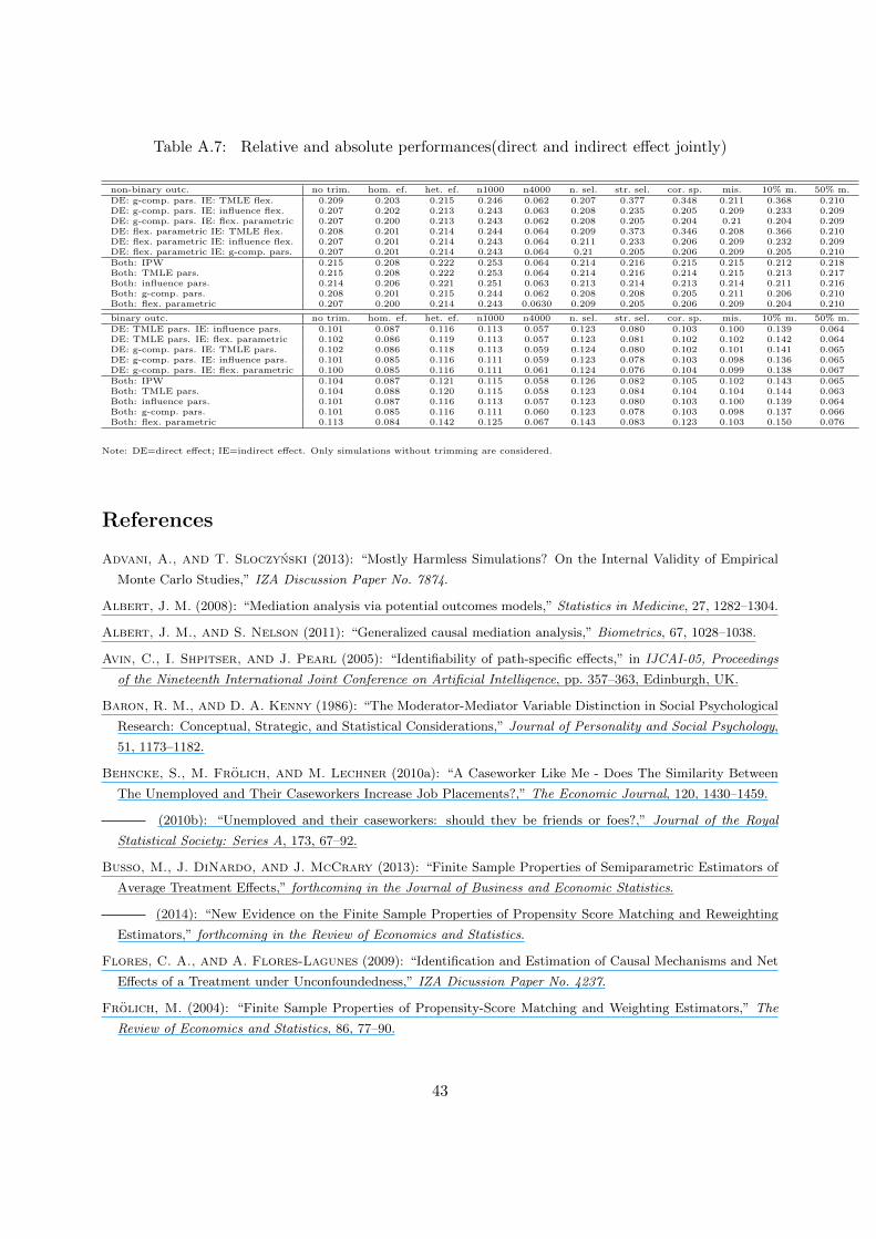
Table A.7: Relative and absolute performances(direct and indirect effect jointly)

non-binary outc. no trim. hom. ef. het. ef. n1000 n4000 n. sel. str. sel. cor. sp. mis. 10% m. 50% m.DE: g-comp. pars. IE: TMLE flex. 0.209 0.203 0.215 0.246 0.062 0.207 0.377 0.348 0.211 0.368 0.210DE: g-comp. pars. IE: influence flex. 0.207 0.202 0.213 0.243 0.063 0.208 0.235 0.205 0.209 0.233 0.209DE: g-comp. pars. IE: flex. parametric 0.207 0.200 0.213 0.243 0.062 0.208 0.205 0.204 0.21 0.204 0.209DE: flex. parametric IE: TMLE flex. 0.208 0.201 0.214 0.244 0.064 0.209 0.373 0.346 0.208 0.366 0.210DE: flex. parametric IE: influence flex. 0.207 0.201 0.214 0.243 0.064 0.211 0.233 0.206 0.209 0.232 0.209DE: flex. parametric IE: g-comp. pars. 0.207 0.201 0.214 0.243 0.064 0.21 0.205 0.206 0.209 0.205 0.210Both: IPW 0.215 0.208 0.222 0.253 0.064 0.214 0.216 0.215 0.215 0.212 0.218Both: TMLE pars. 0.215 0.208 0.222 0.253 0.064 0.214 0.216 0.214 0.215 0.213 0.217Both: influence pars. 0.214 0.206 0.221 0.251 0.063 0.213 0.214 0.213 0.214 0.211 0.216Both: g-comp. pars. 0.208 0.201 0.215 0.244 0.062 0.208 0.208 0.205 0.211 0.206 0.210Both: flex. parametric 0.207 0.200 0.214 0.243 0.0630 0.209 0.205 0.206 0.209 0.204 0.210

binary outc. no trim. hom. ef. het. ef. n1000 n4000 n. sel. str. sel. cor. sp. mis. 10% m. 50% m.DE: TMLE pars. IE: influence pars. 0.101 0.087 0.116 0.113 0.057 0.123 0.080 0.103 0.100 0.139 0.064DE: TMLE pars. IE: flex. parametric 0.102 0.086 0.119 0.113 0.057 0.123 0.081 0.102 0.102 0.142 0.064DE: g-comp. pars. IE: TMLE pars. 0.102 0.086 0.118 0.113 0.059 0.124 0.080 0.102 0.101 0.141 0.065DE: g-comp. pars. IE: influence pars. 0.101 0.085 0.116 0.111 0.059 0.123 0.078 0.103 0.098 0.136 0.065DE: g-comp. pars. IE: flex. parametric 0.100 0.085 0.116 0.111 0.061 0.124 0.076 0.104 0.099 0.138 0.067Both: IPW 0.104 0.087 0.121 0.115 0.058 0.126 0.082 0.105 0.102 0.143 0.065Both: TMLE pars. 0.104 0.088 0.120 0.115 0.058 0.123 0.084 0.104 0.104 0.144 0.063Both: influence pars. 0.101 0.087 0.116 0.113 0.057 0.123 0.080 0.103 0.100 0.139 0.064Both: g-comp. pars. 0.101 0.085 0.116 0.111 0.060 0.123 0.078 0.103 0.098 0.137 0.066Both: flex. parametric 0.113 0.084 0.142 0.125 0.067 0.143 0.083 0.123 0.103 0.150 0.076

Note: DE=direct effect; IE=indirect effect. Only simulations without trimming are considered.

References

Advani, A., and T. Sloczynski (2013): “Mostly Harmless Simulations? On the Internal Validity of Empirical

Monte Carlo Studies,” IZA Discussion Paper No. 7874.

Albert, J. M. (2008): “Mediation analysis via potential outcomes models,” Statistics in Medicine, 27, 1282–1304.

Albert, J. M., and S. Nelson (2011): “Generalized causal mediation analysis,” Biometrics, 67, 1028–1038.

Avin, C., I. Shpitser, and J. Pearl (2005): “Identifiability of path-specific effects,” in IJCAI-05, Proceedings

of the Nineteenth International Joint Conference on Artificial Intelligence, pp. 357–363, Edinburgh, UK.

Baron, R. M., and D. A. Kenny (1986): “The Moderator-Mediator Variable Distinction in Social Psychological

Research: Conceptual, Strategic, and Statistical Considerations,” Journal of Personality and Social Psychology,

51, 1173–1182.

Behncke, S., M. Frolich, and M. Lechner (2010a): “A Caseworker Like Me - Does The Similarity Between

The Unemployed and Their Caseworkers Increase Job Placements?,” The Economic Journal, 120, 1430–1459.

(2010b): “Unemployed and their caseworkers: should they be friends or foes?,” Journal of the Royal

Statistical Society: Series A, 173, 67–92.

Busso, M., J. DiNardo, and J. McCrary (2013): “Finite Sample Properties of Semiparametric Estimators of

Average Treatment Effects,” forthcoming in the Journal of Business and Economic Statistics.

(2014): “New Evidence on the Finite Sample Properties of Propensity Score Matching and Reweighting

Estimators,” forthcoming in the Review of Economics and Statistics.

Flores, C. A., and A. Flores-Lagunes (2009): “Identification and Estimation of Causal Mechanisms and Net

Effects of a Treatment under Unconfoundedness,” IZA Dicussion Paper No. 4237.

Frolich, M. (2004): “Finite Sample Properties of Propensity-Score Matching and Weighting Estimators,” The

Review of Economics and Statistics, 86, 77–90.

43

Gelman, A., and G. Imbens (2013): “Why ask Why? Forward Causal Inference and Reverse Causal Questions,”

NBER Working Paper No. 19614.

Gerfin, M., and M. Lechner (2002): “Microeconometric Evaluation of the Active Labour Market Policy in

Switzerland,” Economic Journal, 112, 854–893.

Hill, W. J., and W. G. Hunter (1966): “A Review of Response Surface Methodology: A Literature Survey,”

Technometrics, 8, 571–590.

Horvitz, D. G., and D. J. Thompson (1952): “A Generalization of Sampling without Replacement from a Finite

Universe,” Journal of the American Statistical Association, 47, 663–685.

Huber, M. (2014): “Identifying causal mechanisms (primarily) based on inverse probability weighting,” Journal

of Applied Econometrics, 29, 920–943.

Huber, M., M. Lechner, and G. Mellace (2014): “Why do tougher caseworkers increase employment? The

role of programme assignment as a causal mechanism,” University of St. Gallen, Department of Economics

Discussion Paper No. 2014-14.

Huber, M., M. Lechner, and C. Wunsch (2013): “The performance of estimators based on the propensity

score,” Journal of Econometrics, 175, 1–21.

Imai, K., L. Keele, and D. Tingley (2010): “A General Approach to Causal Mediation Analysis,” Psychological

Methods, 15, 309–334.

Imai, K., L. Keele, and T. Yamamoto (2010): “Identification, Inference and Sensitivity Analysis for Causal

Mediation Effects,” Statistical Science, 25, 51–71.

Imai, K., and T. Yamamoto (2013): “Identification and Sensitivity Analysis for Multiple Causal Mechanisms:

Revisiting Evidence from Framing Experiments,” Political Analysis, 21, 141–171.

Imbens, G. W. (2004): “Nonparametric Estimation of Average Treatment Effects under Exogeneity: A Review,”

The Review of Economics and Statistics, 86, 4–29.

Kang, J. D. Y., and J. L. Schafer (2007): “Demystifying Double Robustness: A Comparison of Alternative

Strategies for Estimating a Population Mean from Incomplete Data,” Statistical Science, 22, 523–539.

Khan, S., and E. Tamer (2010): “Irregular Identification, Support Conditions, and Inverse Weight Estimation,”

Econometrica, 78, 2021–2042.

Khuri, A. I., and S. Mukhopadhyay (2010): “Response surface methodology,” Wiley Interdisciplinary Reviews:

Computational Statistics, 2, 128–149.

LaLonde, R. (1986): “Evaluating the Econometric Evaluations of Training Programs with Experimental Data,”

American Economic Review, 76, 604–620.

Lechner, M., and C. Wunsch (2013): “Sensitivity of matching-based program evaluations to the availability of

control variables,” Labour Economics, 21, 111–121.

Lunceford, J. K., and M. Davidian (2004): “Stratification and weighting via the propensity score in estimation

of causal treatment effects: a comparative study,” Statistics in Medicine, 23, 2937–2960.

Myers, R. H., A. I. Khuri, and J. Carter, Walter H. (1989): “Response Surface Methodology: 1966-1988,”

Technometrics, 31, 137–157.

Nargelkerke, N. J. D. (1991): “A note on a general definition of the coefficient of determination,” Biometrika,

78, 691–692.

Newey, W. K. (1984): “A method of moments interpretation of sequential estimators,” Economics Letters, 14,

201–206.

44

Pearl, J. (2001): “Direct and indirect effects,” in Proceedings of the Seventeenth Conference on Uncertainty in

Artificial Intelligence, pp. 411–420, San Francisco. Morgan Kaufman.

Robins, J. M. (1986): “A new approach to causal inference in mortality studies with sustained exposure periods

- application to control of the healthy worker survivor effect,” Mathematical Modelling, 7, 1393–1512.

(2003): “Semantics of causal DAG models and the identification of direct and indirect effects,” in In

Highly Structured Stochastic Systems, ed. by P. Green, N. Hjort, and S. Richardson, pp. 70–81, Oxford. Oxford

University Press.

Robins, J. M., and S. Greenland (1992): “Identifiability and Exchangeability for Direct and Indirect Effects,”

Epidemiology, 3, 143–155.

Rubin, D. B. (1974): “Estimating Causal Effects of Treatments in Randomized and Nonrandomized Studies,”

Journal of Educational Psychology, 66, 688–701.

(2004): “Direct and Indirect Causal Effects via Potential Outcomes,” Scandinavian Journal of Statistics,

31, 161–170.

Tchetgen Tchetgen, E. J., and I. Shpitser (2012): “Semiparametric theory for causal mediation analysis:

Efficiency bounds, multiple robustness, and sensitivity analysis,” The Annals of Statistics, 40, 1816–1845.

Ten Have, T. R., M. M. Joffe, K. G. Lynch, G. K. Brown, S. A. Maisto, and A. T. Beck (2007): “Causal

mediation analyses with rank preserving models,” Biometrics, 63, 926–934.

Tingley, D., T. Yamamoto, K. Hirose, K. Imai, and L. Keele (2014): “Mediation: R package for causal

mediation analysis,” Journal of Statistical Software, 59, 1–38.

van der Laan, M., and D. Rubin (2006): “Targeted maximum likelihood learning,” International Journal of

Biostatistics, 2.

Waernbaum, I. (2012): “Model misspecification and robustness in causal inference: comparing matching with

doubly robust estimation,” Statistics in Medicine, 31, 1572–1581.

Zhao, Z. (2004): “Using Matching to Estimate Treatment Effects: Data Requirements, Matching Metrics, and

Monte Carlo Evidence,” Review of Economics and Statistics, 86, 91–107.

Zheng, W., and M. J. van der Laan (2012): “Targeted Maximum Likelihood Estimation of Natural Direct

Effects,” The International Journal of Biostatistics, 8, 1–40.

45