The efficiency of trading halts: Emerging market evidence

International Journal of Banking and Finance

| Issue 2Volume 5 Article 7

3-1-2008

The efficiency of trading halts: Emerging marketevidenceObiyathulla I. BachaInternational Islamic University Malaysia

Mohamed Eskandar S. A. RashidInternational Islamic University Malaysia

Roslily RamleeInternational Islamic University Malaysia

This Journal Article is brought to you by the Faculty of Business at ePublications@bond. It has been accepted for inclusion in International Journal ofBanking and Finance by an authorized administrator of ePublications@bond. For more information, please contact Bond University's RepositoryCoordinator.

Recommended CitationBacha, Obiyathulla I.; Rashid, Mohamed Eskandar S. A.; and Ramlee, Roslily (2008) "The efficiency of trading halts: Emergingmarket evidence," International Journal of Banking and Finance: Vol. 5: Iss. 2, Article 7.Available at: http://epublications.bond.edu.au/ijbf/vol5/iss2/7

http://epublications.bond.edu.au/ijbf

http://epublications.bond.edu.au/ijbf/vol5/iss2

http://epublications.bond.edu.au/ijbf/vol5

http://epublications.bond.edu.au/ijbf/vol5/iss2/7

http://epublications.bond.edu.au

mailto:[email protected]

mailto:[email protected]

The International Journal of Banking and Finance, 2007/08 Vol. 5. Number 2: 2008: 125-148 125

THE EFFICIENCY OF TRADING HALTS: EMERGING MARKET EVIDENCE

Obiyathulla I. Bacha, Mohamed Eskandar S. A. Rashid and Roslily RamleeInternacional Islamic University Malaysia

Abstract

This paper reports new findings on the price effect from trading halts - both voluntary and mandatory - over 2000-04 in an emerging share market, Malaysia. Based on our overall sample, trading halts lead to positive price reaction, increased volume, and increased volatility. We found evidence of information leakage resulting in a significant difference between voluntary and mandatory halts as well as the type of news released during halts to warrant such an impact. The duration of the halt has an isolated impact and is largely inconsequential. The frequency of halts does not seem to matter.

Keywords: Trading Halts, Price, Efficiency, and MalaysiaJEL classification: G14

1. Introduction

The efficacy of trading halts (or trading suspensions) in overcoming informational asymmetries remains a controversy. Being that it is a temporary suspension of trading in a stock, a trading halt is essentially a signal by the exchange that disequilibrium exists or is expected to exist. That disequilibrium may be the result of an order imbalance or more likely due to pending news. The halt therefore is a “time-out” for the adjustment of prices during real or perceived, temporary disequilibria. Though numerous studies have been undertaken in various markets, there appear to be no consensus on the usefulness of trading halts/suspensions. The objective of a trading halt, whether voluntary (one initiated by the firm) or mandatory (one imposed by regulators), is to always ensure a fair access to information and price formation. Therein lies the debate of whether that objective is achieved or not. Supporters of trading halts propose that calling a halt to trading just prior to the voluntary or forced release of critical information enhances price formation/discovery by ensuring equitable dissemination and assimilation.

Often denoted as the Price Efficiency Hypothesis of Trading Halts1, the rationale is that since a trading suspension gives time for investors to better digest the impact of news, price dispersions should be smaller, implying lower volatility

1 See Chen H, Chen H, and Valerios, N(2003).

IJBF

1

Bacha et al.: The efficiency of trading halts: Emerging market evidence

Produced by The Berkeley Electronic Press, 2008

126 The International Journal of Banking and Finance, 2007/08 Vol. 5. Number 2: 2008: 125-148

and a higher degree of price efficiency upon reopening. Opponents of trading halts using the “learning through trading models” would argue that since a halt prevents trading during the suspension period, excess volatility is not necessarily being avoided, but rather, merely postponed. Based on the logic of “learning through trading models”, reopening prices would be noisy. This implies reduced pricing efficiency and increased volatility.

Just as the arguments have been diametric, empirical evidence thus far have been mixed. Most empirical work on firm-specific trading halts had focused on the three key variables most likely to be affected by a halt: • excess returns• price/returns volatility• trading volume.

While the behavioral findings of these three variables, post-halt, provide a mixed picture, studies that had refined the analysis had produced interesting results. Indeed, the mixed evidence begs for refinement. It appears that factors driving the halt may be just as important as the halt itself in explaining the post-halt behavior of the three variables.

Our examination of existing literature points to at least four parameters associated with a trading halt that could throw additional light on the evidence. Firstly, we will examine the reason for the halt/suspension on whether it was voluntarily or mandatorily imposed. Secondly, we will take a look at the type of news or information released during the halt, whether it constitutes good, bad, or neutral news. Thirdly, we will also take into account the duration of the halt. Lastly, the fourth parameter would be the frequency of the stock in question, whether the halt constitutes a first (single) halt or one of several- (multiple) halts. While earlier studies had focused on the impact of the halt/suspension alone, later studies had brought to bear at least one or more of the above parameters.

1.1 Motivation Trading halts by definition are ‘disruptive’ events that are almost always associated with events that have the potential to cause abrupt or extreme moves. While market-wide, trading halts are indeed rare and unpredictable events2, whereas firm specific trading halts are not. Indeed, as emerging markets have expanded their market capitalization, firm specific halts have been more frequent. There have been more than 300 trading suspensions over the last five-years at Bursa Malaysia. Despite the fact that trading halts appear to be a fairly common occurrence, we are unaware of any systematic studies of the phenomenon in Malaysia. This absence provides the motivation and justification for this study.

As is the case with other markets, trading halts or temporary suspensions of listed stocks in Bursa Malaysia may be voluntary or mandatorily imposed. The administrative framework for temporary suspensions is outlined in Chapter 16 of Bursa Malaysia’s Listing Guidelines. While a listed issuer through a request to the exchange initiates voluntary suspensions, it remains the Exchange’s discretion to grant such a suspension. Mandatory suspensions can be initiated either by the

2 Such as the trading halt on the NYSE following the September 11 attacks.

2

International Journal of Banking and Finance, Vol. 5, Iss. 2 [2008], Art. 7



Exchange or the Securities Commission (SC). The SC can notify the exchange to suspend a stock from trading if it deems the issuer to be in breach or failure in compliance with the Securities Industry Act 1983, the Securities Commission Act 1993, or when the Commission feels that “it is necessary or expedient in the public interest or where necessary for the protection of investors”.

Section 16.02 of the Listing Guideline provides the Exchange the right to suspend at any time the trading of any listed security if the issuing company is undergoing a substantial corporate exercise, capital restructuring, stock conversion, or exercise in the event of any breach of the listing requirements.

Additionally; the exchange may also mandatorily suspend trading of a stock if in its opinion, “it is necessary or expedient in the interest of maintaining an orderly and fair market in securities traded on the Exchange”. As is evident, both voluntary and mandatory suspensions can be the result of a wide range of reasons. While authorities obviously have broad powers to halt trading, companies as well can request the voluntary suspension of their stock for any number of reasons.

In this paper, we examine a total of 291 firm-specific trading halts that occurred on Bursa Malaysia over the five-year period from 2000 to 2004. The paper is divided into four sections. Section 2 provides a review of the literature, where as Section 3 lays out our research questions, describing the data, research, design, and methodology implemented. Section 4 presents the analysis of our results, while Section 5 concludes the paper with our evaluation of the efficacy of trading halts in the Malaysian context, along with providing implications for policy.

2. Literature Review

Much of the research interest in trading halts appears to have originated from the seminal work of Hopewell and Schwartz (1978). In that study of several hundred firm specific halts on the NYSE, they had reported three key findings:1. There exists a permanent price adjustment in response to new information

released2. There exists an anticipatory price behavior consistent with insider trading and

information leakage. 3. Post-suspension price behavior presents little, if any opportunity for systematic

trading profits.Additionally, they had also reported that suspensions of longer duration

typically result in price adjustments of greater magnitude. Most other U.S. based studies on trading halts have also examined their impact on trading volume and volatility. At least three such studies document significant increases in both volume and volatility, post-halt. Lee, Ready, & Seguin (1994) had compared the impact of trading halts versus ‘pseudo-halts’, which are non-halt control periods on volume and volatility. They had concluded that rather than reducing both volume and volatility, the number of trading halts had increased. For the first, full day, post-halt, they had found trading volume to be 230% higher with volatility between 50 - 115% higher compared to pseudo-halts. Further, the persistently high volume for days +2 and +3 does not seem to fit the “learning through trading model”.

3



https://www.researchgate.net/publication/4992337_Volume_Volatility_and_New_York_Stock_Exchange_Trading_Halts?el=1_x_8&enrichId=rgreq-4c3d2692bf46ee8dcae2236e4d8dd616-XXX&enrichSource=Y292ZXJQYWdlOzQxNDU4OTg5O0FTOjE1NDE4NTM2NjUxMTYyM0AxNDEzNzcyMDY0NjY0


These results are consistent with the earlier findings of Ferris, Kumar, and Wolfe (1992), who had examined the impact of mandatory SEC ordered trading halts. They had found that volume and volatility tended to be higher than normal in the pre-suspension period with the trend continuing in the immediate post-suspension period. They had also reported a permanent devaluation of stocks during the suspension with the extent of the devaluation dependent on the announced reason for the halt. Examining trading halts on the NASDAQ, Christie, Corwin, and Harris (2002) had reported significantly higher volatility, volume, and bid-ask spreads in the period following halts. Comparing their results with those based on the NYSE and others, they had found trading halts to have important effects, independent of the market structure and the specific halt mechanism used.

Yet, other U.S. studies (while reporting similar findings with regards to price, volatility, and volume) have examined additional parameters. In addition to the argument that suspensions are almost always ‘bad news’,3 Howe and Schlarbaum (1986) had shown the existence of a correlation between the length of suspension (measured in trading days) and cumulative, abnormal returns. Longer suspensions coincide with bigger, negative residuals. Chen, Chen, and Valerios (2003) had examined the intraday data for 1992 of NYSE stocks. Their findings had showed that the type and significance of news determines the benefit from the trading halt. They had argued that halts can be beneficial in light of significant news coming to fruition. However, when a halt is called, pending a news release of little significance, the halt actually injects more noise into prices, undermining price discovery.

A number of papers have examined trading halts in other countries. In analyzing stock specific suspensions on the London Stock Exchange, Kabir (1994) had pointed towards anticipatory behavior, pre-halt, arguing that the presence of significantly positive abnormal returns up to a month following the reinstatement of trading had implied one of two things: • the complete impact of new information release takes place gradually• not all-relevant information is disclosed during the halt.

Wu (1998) had also examined the issue of information dissemination during halts for the Hong Kong market. He had found that mandatory suspension shows more effectiveness in disseminating information than voluntary suspensions. His findings about price reaction, volatility, and volume are largely in sync with that of U.S. studies. Tan and Yeo (2003) had studied the impact surrounding the type of news on voluntary suspensions in Singapore. Grouping firm-initiated suspensions into ‘favorable’ and ‘unfavorable’ news, they had found that while the first group showed significant, positive, abnormal returns around the event date, the latter group had suffered a prolonged decline. They had also pointed out that the much higher post-suspension volatility of returns implies the rationale behind voluntary suspensions to be a release of price sensitive info rather than to curb existing volatility.

At least one study of the Italian market (Borsa Italiana) and another of the Portuguese market had produced results in conformity with findings elsewhere that

3 They had found that 80% of suspended securities have suffered a substantial devaluation.

4



https://www.researchgate.net/publication/24070638_Voluntary_Trading_Suspensions_in_Singapore?el=1_x_8&enrichId=rgreq-4c3d2692bf46ee8dcae2236e4d8dd616-XXX&enrichSource=Y292ZXJQYWdlOzQxNDU4OTg5O0FTOjE1NDE4NTM2NjUxMTYyM0AxNDEzNzcyMDY0NjY0


volume and volatility are higher, post-halt. Generalizing across studies conducted in different markets, the broad conformity of results implies that market microstructures do not matter. What appears to matter is the type of information released, duration of the halt, and whether they are voluntarily or mandatorily imposed.

3. Methodology and Data

3.1 Research DesignIn line with previous works cited in Section 2, we begin by examining the variables commonly impacted by trading halts (i.e., stock price reaction, volatility of returns, and trading volume). Since the leakage of information has a direct impact on the efficacy of halts, we also explore for the evidence of such a leakage. In addition to these four factors, as the first study on trading halts in the Malaysian context, we seek to add to the comprehensiveness of the study by including four, related dimensions:1. type of halt (whether voluntary or mandatory)2. category of news released (whether good, bad, or neutral)3. duration of halt4. frequency (whether the halt constitutes a single halt for the stock or is one of

several). Previous studies have included one or more of these four dimensions when

examining price, volume, and volatility. Results have shown that these dimensions could have a material effect on the overall effectiveness of trading halts. Thus, we seek to examine each of the four standard variables of price reaction, volatility, volume, and information leakage within each of the four dimensions. For example, we seek to determine whether or not the price reaction, volatility, volume, and extent of information leakage are any different for voluntary versus mandatory halts, or when the news released is of a different type. Given this objective, we frame the following 5 broad research questions: 1. What is the overall impact of trading halts on stock returns, volatility, and

volume? 2. How different are these results when the halt is voluntary as opposed to

mandatory?3. What difference if any, does the type of news released make?4. Does the duration of the halt/suspension have any influence?5. Are the results of single halts any different from those of multiple halts?

Differentiating between voluntary and mandatory halts is fairly straightforward. Where the issuing firm had requested a halt, it is the former; where either Bursa Malaysia or the SC imposed the halt, it is a mandatory halt.

Unlike Ferris et. al., (1992) or Tan and Yeo (2003), who had used the positive/negative daily abnormal returns prior to a halt to classify their sample in the ‘good’ or ‘bad’ news category, we examine the news released during the halt4. A judgment is then made on the category of news. Most were fairly straightforward.

4 Or news released just after the announcement of the halt.

5



https://www.researchgate.net/publication/4759623_The_Effect_of_SEC-Ordered_Suspensions_on_Returns_Volatility_and_Trading_Volume?el=1_x_8&enrichId=rgreq-4c3d2692bf46ee8dcae2236e4d8dd616-XXX&enrichSource=Y292ZXJQYWdlOzQxNDU4OTg5O0FTOjE1NDE4NTM2NjUxMTYyM0AxNDEzNzcyMDY0NjY0



Announcements reporting increased earnings, profits, higher dividends, the winning of new contracts, etc., were categorized as ‘good’ news. The opposite would constitute ‘bad’ news. Where the news was deemed to be neither, for example, unchanged earnings, etc., or where we were unsure, we classified it in the ‘neutral’ news category. During the duration of the halt, we had three classifications. A halt is classified to be:1. ‘short’ if the halt is for one trading day5

2. ‘medium’ if the halt has a duration between 2 to 5 trading days.3. ‘long’ if the halt has a duration longer than 5 trading days.

Finally, in determining whether a halt belongs to the single or multiple suspension category, we used a one-year cut-off. If a stock was suspended more than once within a one-year period, we classified it in the multiple suspension category.

Our dataset consists of 291 trading halts that occurred on Bursa Malaysia over the five-year period from 2000 to 2004. Of the 291 total trading halts, the issuing firms had voluntarily requested 263 halts, whereas 28 trading halts were mandatory halts imposed by either Bursa Malaysia or the SC. The basis of our analysis is the daily closing price data of each sample for a 120-trading-day period around the announcement date of the halt. That is 60 days immediately prior to the announcement date and 60 days following the resumption of trading. (All daily price data were sourced from Bloomberg.) Others, such as information on announcements and firm specific information, were from Bursa Malaysia publications and newspapers.

3.2 MethodologyIn line with almost all-previous work in this area, we used an event-study framework. Thus, in examining the price reaction to an announcement of a trading halt, we had computed the Abnormal Returns (AR) and Cumulative Abnormal Returns (CAR) for the two 60-day period windows for each firm. Where necessary, we also examined the smaller windows within the 60-day windows. The daily CAR is computed as:

(1)

where, the Daily Abnormal Return on day t for stock i is determined as:

AR

i,t = AR

i,t - R

i,t (2)

The Abnormal Return ARi,t is the difference of day t’s actual return of R

i,t less the

expected return of Ri,t where:

(3)

RM equals the returns of the KLSE CI (Kuala Lumpur Stock Exchange Composite Index).

5 The shortest duration of halts in Malaysia is one day.

ˆ

ˆ

∑=

==t

ttiti NIiARCAR

1,, .,.........

tiiti RMBR^^

,

^+= α

6




Beta was estimated using daily stock and market returns for the 60-day period: -61 to -120 pre-halt announcement.

Next, we computed the daily mean Abnormal Return (that is, the average abnormal return across all samples on day t).

The daily mean abnormal return (MAR) is:

(4)

and Variance

(5)

In addition to computing the daily CARs for each of our sample companies, we

computed the mean overall CARs for all sample companies for each window period.

The Mean Cumulative Abnormal Return (MCAR) is determined as:

(6)

In determining the daily returns volatility for each window period, we first determined the volatility of returns across all sample firms by day (t). This is computed as:

Where τit is the % return for firm i, on day t, CP

it is the closing price for stock of firm

i on day t.

(7)

For trading volume, we used the absolute number of stocks traded for each sample firm on day t.

(8)

Where TVt is the mean trading volume across all sample firms on day t, tv

i,t is the

trading volume of stock for firm i on day t.

TtN

AR

MAR

N

titi

t ...........,1,

==∑

=

TtN

ARVAR

MARVAR

N

titi

t ...........,1

)(

)(2

,

==∑

=

TtN

CAR

N

CAR

MCAR

N

iti

N

titi

t ...........,1

)(

2

1,,

==∑∑

==

( )[ ] 100Re 1,1,,, xCPCPCP titititi −−−=τ

( )( )2

,Re

ReN

tVar

tVar

N

titi

t

∑==

NtvTVN

titit ⎟⎟⎠

⎞⎜⎜⎝

⎛= ∑

=,

7




While CARs and Abnormal Returns are used to determine the impact of trading halts on price behavior, we examined the impact on returns volatility and trading volume. Firstly, we employed the standard means test using the t-statistics and the non-parametric Wilcoxon signed rank test (the latter test assumes the distribution is unknown or non-normal). Additionally, the Wilcoxon test uses the median to avoid test misspecifications that may arise from asymmetry in cross-sectional tabulations and non normal distribution. In comparing volatility, pre- and post-halt, we compared the variance between the samples using the F-test instead of the t-test. Previous studies have shown that the results drawn from the event study can be sensitive to sample size and estimation period6. To avoid any bias that may arise from the selection of a pre- and post-event period, we examined the results by varying the window periods and by dividing the sample into those additional dimensions mentioned above (categorization by type of halt, type of news, duration, etc.).

3.3 Testable HypothesesA number of testable hypotheses about the impact of halts on price, volatility, and volume may be inferred from previous literature.(i) Price Effect: a trading halt can either enhance price discovery by providing

participants a “time-out” to assimilate impending new information as its proponents argue, or interfere with price discovery as its opponents point out. Either way, more important than the halt is the information released during the halt. A company calls for a voluntary trading halt of its shares in order to release new information. In the case of a mandatorily required halt, even if no information is forthcoming immediately following the halt, the mere fact that authorities had stopped trading in the stock is a signal that there is a substantive problem. Thus, in the absence of information leakage, the impact of trading halts on price behavior would be in one of the following three forms:1. if information released is insignificant, there should be no abnormal

returns on trading resumption.2. if the information released is significant, a price reaction should occur

(the kind of reaction being dependent on the type of news).3. if the market had anticipated the information released during the halt, then

we should expect ‘price continuation’; i.e. prices continue to move in the same direction. On the other hand, if the news released was unanticipated, then a price reversal could be the case.

Thus, with these three hypotheses, we test the following:1. whether trading halts are significant events where price behavior is

concerned 2. whether post-halt price behavior is dependent on the type of news 3. whether information released during halts merely reinforce anticipations

or otherwise.

6 Coutts, Mills, and Roberts (1994), cited in Wu (1998)

8




(ii) Effect on Returns Volatility: if trading halts require a time-out for participants to properly evaluate information during real or perceived market disequilibrium, then one should expect lower returns volatility, post-halt. Alternatively, going by the logic of “learning through trading models”, the absence of transactions should exacerbate the uncertainty/disequilibria, thereby causing an increase in returns volatility, post-halt.

(iii) Effect on Trading Volume: there are two reasons why halts can be expected to have an impact on traded volume. Firstly, the release of new information may require market participants to adjust their positions/exposure in the stock. Volume increases, post-halt, as the stock changes hands. Secondly, if one assumes trading in normal times to be evenly distributed over time, then it can be expected that when trading resumes following a halt, volume ought to be higher in order to compensate for the disruption. This also implies that the longer the trading halt, the greater the impact would be on volume.

4. Results and Analysis

Given the numerous permutations involved in our analysis, for ease of elucidation, we presented our results by the four variables of interest: • Price• Returns Volatility• Volume• Information Leakage.

Following an overall examination of the impact of trading halts on each of these variables, we then presented the results of our analysis examining each variable by the four dimensions: • type of halt• type of news released• duration of halt• frequency.

The breakdown of sample size within each of these subcategories is shown in Table 6.

Table 6: Breakdown of Voluntary Halts Sample by Category

Note: The total number of Voluntary halts in our sample was 263. The Mandatory halts which had a sample size of 28 firms was not subdivided by category since these are irrelevant. Mandatorily ordered halts are by definition ‘bad’ news, are of long duration and are only subjected to a single halt.

Type of news released Duration of halt Frequency of halt

Good news 120 Short 162 Single 106

Neutral news 120 Medium 92 Multiple 157

Bad news 23 Long 9

Total 263 Total 263 Total 263

9




4.1 Price EffectTable 1 and Figure 1 show the results of our analysis of daily Cumulative Abnormal Returns (CARs) for the 120-day period surrounding the halt announcement. Table 1 shows the Mean CARs (MCARs) for 3 pairs of Window periods, 60 days pre/post; 30 days pre/post; and 5 days pre/post announcement. The results of the paired samples t-test and the non-parametric Wilcoxon Signed Ranks test for difference in means. The probability levels are also shown.

Overall, for the full sample of 291 firm-specific halts, MCARs are higher for all 3 windows in the post-halt period. In other words, there is a positive price reaction once a halt is lifted. There is a big jump in the MCAR for the +5 day window. This is followed by a steady rise in the two subsequent window periods +30 and +60. Thus, prices are much higher 60 days after the resumption of trading relative to where they were 60 days before the announcement of halt. Both statistical tests (t and Wilcoxon) showed post-halt MCARs to be significantly higher relative to their pre-halt windows at the 5% level. Interestingly enough, when observing the MCARs for the 3 pre-halt periods, we saw a steady increase as we approached announcement date. Pre-halt MCAR is at it’s maximum for the -5 day window. This steady buildup in prices is also clearly evident in Figure 1 that plots daily CARs.

Figure 1: Daily CARs for Overall Sample; Voluntary and Mandatory Halts

4.2 Price Effect by Type of HaltsThe subsequent two columns show the results when the overall sample is separated into Voluntary and Mandatory halts. Recall that our sample constituted of 263 voluntary and 28 mandatory halts. Looking at the results for the voluntary halts, we see results very similar to the overall. All 3 post-halt MCARs are higher and significant for the 60 and 30-day windows. We also see the marked increase in MCAR just prior to the announcement. The MCAR for the -5 day window is more than 5 times larger than that of the -60 day window. The results for voluntary halts are very similar to that of the overall sample. That should not be surprising given that the large majority (almost 90%) of our sample constituted of voluntary halts.

-5

0

5

10

15

20

25

30

35

-80 -60 -40 -20 0 20 40 60 80

DAYS

CARs

OVERALL

VOLUNTARYMANDATORY

10



The International Journal of B

anking and Finance, 2007/08 V

ol. 5. Num

ber 2: 2008: 125-148

135

Table 1: Cumulative Abnormal Returns by Category

Window Period

Price Effect By News By Duration Frequency

Overall Voluntary Mandatory Good Neutral Bad Short Med Long Single Multiple

(-60 to -1) 1.0770 .9846 1.9456 2.3463 2.6350 -1.12029 2.0517 .3981 -12.4045 .9547 1.1184(+1 to +60)

8.8800 8.0651 16.5343 14.8738 2.7264 .4066 10.5503 4.2919 2.3364 11.4132 7.2065

(-30 to -1) 2.0115 1.9196 2.8749 3.7162 .6580 -.8714 3.6891 .5252 -15.7090 1.7727 2.2686(+1 to +30)

7.3775 6.815 12.6598 12.8591 2.7632 -3.5775 9.3678 3.6907 -6.6638 10.5240 5.4042

(-5 to -1) 4.8120 5.143 1.6954 6.1787 4.8091 1.4904 7.6503 2.771 -15.4385 5.7903 4.5031

(+1 to +5) 6.7212 6.253 11.112 10.4326 3.5251 -1.3127 9.1165 3.6264 -17.3855 9.3882 5.7221

T-Stat

-62.680(000)

-50.949(.000)

-16.762(.000)

-81.080(.000)

-9.231(.000)

-2.544(.014)

-43.114(.000)

-13.947(.000)

-7.275(.000)

-50.665(.000)

-42.387(.000)

-25.200(000)

-18.766(.000)

-15.507(.000)

-54.777(.000)

-4.294(.000)

4.708(.000)

-16.533(.000)

-7.130(.000)

-5.405(.000)

-25.960(.000)

-10.523(.000)

-4.187(014)

-2.656(.057)

-7.737(.002)

-8.516(.001)

2.626(.058)

6.647(.003)

-4.111(.015)

-1.256(.277)

.667(.553)

-6.308(.003)

-4.940(.008)

Wilcoxon Z-Stat

-6.736 (.000)

-6.736 (.000)

-6.736(.000)

-6.736(.000)

-5.904(.000)

-2.245(.025)

-6.736(.000)

-6.729(.000)

-5.382(.000)

-6.736(.000)

-6.736(.000)

-4.782 (.000)

-4.782 (.000)

-4.782(.000)

-4.782(.000)

-3.466(.001)

-3.651(.000)

-4.782(.000)

-4.391(.000)

-4.184(.000)

-4.782(.000)

-4.782(.000)

-2.023(.043)

-1.753 (.080)

-2.023(.043)

-2.023(.043)

-1.753(.080)

-2.023(.043)

-2.023(.043)

-1.214(.225)

-.730(.465)

-2.023(.043)

-2.023(.043)

The table shows the Mean CARs by window period for the different categories. T-stat values shown are for paired sample test the prob. values are shown below in brackets.

11




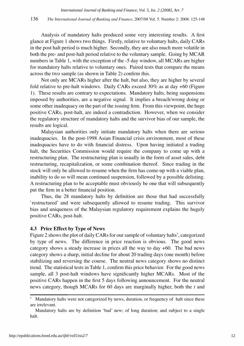
Analysis of mandatory halts produced some very interesting results. A first glance at Figure 1 shows two things. Firstly, relative to voluntary halts, daily CARs in the post halt period is much higher. Secondly, they are also much more volatile in both the pre- and post-halt period relative to the voluntary sample. Going by MCAR numbers in Table 1, with the exception of the -5 day window, all MCARs are higher for mandatory halts relative to voluntary ones. Paired tests that compare the means across the two sample (as shown in Table 2) confirm this.

Not only are MCARs higher after the halt, but also, they are higher by several fold relative to pre-halt windows. Daily CARs exceed 30% as at day +60 (Figure 1). These results are contrary to expectations. Mandatory halts, being suspensions imposed by authorities, are a negative signal. It implies a breach/wrong doing or some other inadequacy on the part of the issuing firm. From this viewpoint, the huge positive CARs, post-halt, are indeed a contradiction. However, when we consider the regulatory structure of mandatory halts and the survivor bias of our sample, the results are logical.

Malaysian authorities only initiate mandatory halts when there are serious inadequacies. In the post-1998 Asian Financial crisis environment, most of these inadequacies have to do with financial distress. Upon having initiated a trading halt, the Securities Commission would require the company to come up with a restructuring plan. The restructuring plan is usually in the form of asset sales, debt restructuring, recapitalization, or some combination thereof. Since trading in the stock will only be allowed to resume when the firm has come-up with a viable plan, inability to do so will mean continued suspension, followed by a possible delisting. A restructuring plan to be acceptable must obviously be one that will subsequently put the firm in a better financial position.

Thus, the 28 mandatory halts by definition are those that had successfully `restructured’ and were subsequently allowed to resume trading. This survivor bias and uniqueness of the Malaysian regulatory requirement explains the hugely positive CARs, post-halt.

4.3 Price Effect by Type of NewsFigure 2 shows the plot of daily CARs for our sample of voluntary halts7, categorized by type of news. The difference in price reaction is obvious. The good news category shows a steady increase in prices all the way to day +60. The bad news category shows a sharp, initial decline for about 20 trading days (one month) before stabilizing and reversing the course. The neutral news category shows no distinct trend. The statistical tests in Table 1, confirm this price behavior. For the good news sample, all 3 post-halt windows have significantly higher MCARs. Most of the positive CARs happen in the first 5 days following announcement. For the neutral news category, though MCARs for 60 days are marginally higher, both the t and

7 Mandatory halts were not categorized by news, duration, or frequency of halt since these are irrelevant. Mandatory halts are by definition ‘bad’ new; of long duration; and subject to a single halt.

12




Wilcoxon tests show price performance in the 5 days following announcement to be no different from the 5 days immediately prior.

Figure 2: Daily CARs by Type of News

Thus, the price reaction in the neutral news category is largely muted. The MCARs for bad news category is already in negative territory for the -60 and -30 day windows. However, the MCARs show a positive build-up just before announcement as seen from the -5 days window. Of course, all these positive build-ups are erased following the announcement. The MCARs are sharply negatively for the +5 and +30 day windows.

The price reaction seen here is in line with expectations. What is interesting to note is the build-up of prices just before announcement. Though Table 1 shows this to be true for all 3 news categories, the build-up is most obvious in Figure 2 for the Good and Neutral news categories.

4.4 Price Effect by Duration of HaltsWe next examined whether the duration of the halt matters for a price reaction. The results in Table 1 confirmed the relevance. For short duration halts, MCARs for all 3 windows are significantly higher, post-halt. We saw two obvious differences for Medium term halts. The MCARs, though higher, post-halt, are all lower relative to the ones we saw for short duration halts. Secondly, both tests show MCARs to be no different between the -5 and +5 day windows, implying that there is no significant initial price reaction when trading resumes. In sharp contrast to short and medium duration halts, long term halts show very different price behavior. MCARs are already negative for all 3 windows even before the halt. When trading resumes, initially, there is a sharp, negative reaction. The stocks experience a MCARs of -17% within the first week. This decline however abates with time. Though the +5 and +30 day windows have negative MCARs, it is marginally positive for +60

-10

-5

0

5

10

15

20

25

-80 -60 -40 -20 0 20 40 60 80

DAYS

CAR

GOOD

NEUTRAL

BAD

13




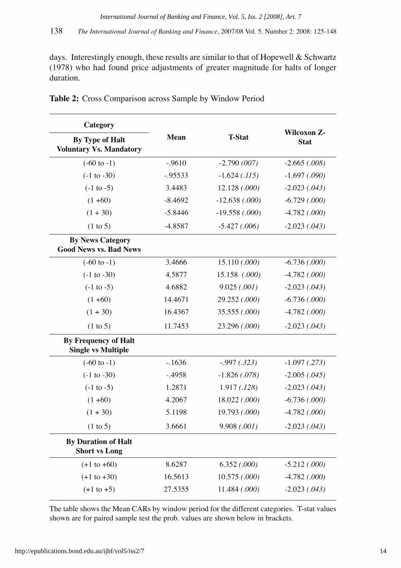
days. Interestingly enough, these results are similar to that of Hopewell & Schwartz (1978) who had found price adjustments of greater magnitude for halts of longer duration.

Table 2: Cross Comparison across Sample by Window Period

Category

Mean T-StatWilcoxon Z-

StatBy Type of Halt Voluntary Vs. Mandatory

(-60 to -1) -.9610 -2.790 (007) -2.665 (.008)

(-1 to -30) -.95533 -1.624 (.115) -1.697 (.090)

(-1 to -5) 3.4483 12.128 (.000) -2.023 (.043)

(1 +60) -8.4692 -12.638 (.000) -6.729 (.000)

(1 + 30) -5.8446 -19.558 (.000) -4.782 (.000)

(1 to 5) -4.8587 -5.427 (.006) -2.023 (.043)

By News Category Good News vs. Bad News

(-60 to -1) 3.4666 15.110 (.000) -6.736 (.000)

(-1 to -30) 4.5877 15.158 (.000) -4.782 (.000)

(-1 to -5) 4.6882 9.025 (.001) -2.023 (.043)

(1 +60) 14.4671 29.252 (.000) -6.736 (.000)

(1 + 30) 16.4367 35.555 (.000) -4.782 (.000)

(1 to 5) 11.7453 23.296 (.000) -2.023 (.043)

By Frequency of HaltSingle vs Multiple

(-60 to -1) -.1636 -.997 (.323) -1.097 (.273)

(-1 to -30) -.4958 -1.826 (.078) -2.005 (.045)

(-1 to -5) 1.2871 1.917 (.128) -2.023 (.043)

(1 +60) 4.2067 18.022 (.000) -6.736 (.000)

(1 + 30) 5.1198 19.793 (.000) -4.782 (.000)

(1 to 5) 3.6661 9.908 (.001) -2.023 (.043)

By Duration of HaltShort vs Long

(+1 to +60) 8.6287 6.352 (.000) -5.212 (.000)

(+1 to +30) 16.5613 10.575 (.000) -4.782 (.000)

(+1 to +5) 27.5355 11.484 (.000) -2.023 (.043) The table shows the Mean CARs by window period for the different categories. T-stat values shown are for paired sample test the prob. values are shown below in brackets.

14




The above results, together with those in Table 2 comparing MCARs across categories, imply a link between duration of halt and price behavior, post-halt. Generally, it appears from our results that shorter duration halts experience positive price reactions, post-halt, whereas long duration halts experience the opposite. These results are sensible when we consider the fact that all halts are disruptive, with longer term ones even more so. Even if the halt was voluntarily requested, issuing companies will only want longer halts if they have more complex issues to solve. Complicated problems will require a longer time-out. The negative MCARs we saw for all three pre-halt windows would imply that may indeed be the case. Companies needing long-duration halts already experience problems; thus they need time to sort these out.

Our final analysis with regards to price effect was to see if the frequency of halts had any different price behavior. The results in Table 1 show similar price reactions, post-halt. When the MCARs are compared between the two categories (Table 2) for matched window periods, we see no difference, pre-halt, but when trading resumes, single halts outperform multiple halts. This out-performance is significant at the 5% level by both the parametric and non-parametric tests.

4.5 Evidence of Information LeakageScrutinizing the MCARs in Table 1 shows an interesting feature. For almost all categories of analysis, we see a marked increase in MCARs for the -5 day window. Such a pattern is also clearly visible from the daily CARs plotted in Figures 1 & 2. This appears to be a tentative evidence of information leakage. The presence of such leakage has been documented for several markets in the previous studies cited in Section 2. To seek confirmation of such leakages for Bursa Malaysia, we examined the MCARs for any possible significant differences across two different window periods, 20 days before halt. The first is the 10-day pre-halt window (-20 to -11) and the final 10 days (-10 to -1). Essentially, we want to see if there is a significant price change in the last 2 weeks leading to the halt, relative to the 2 weeks prior. The results are shown in Table 3. At the 5% level, both the parametric and non-parametric tests show consistent results.

For the overall sample of 291 companies, MCARs for the last 10 days was indeed significantly higher than the 10 previous days. This initial evidence of leakage was reinforced when we examined the voluntary and mandatory sub-segments. Voluntary halts have MCARs almost 3 times higher in the final 10 days than the previous 10-day window. Mandatory halts on the other hand, have MCARs more than 3 times lower in the last 10 days. The differences are statically significant for both cases.

When the same 10-day windows were examined across the different type of news categories, MCARs for the latter window period was significantly higher in all cases, even for the bad news category. What is interesting is that when we go from good to neutral to bad news categories, the MCARs steadily reduce. Finally, both the single and multiple suspension categories had significantly higher MCARs for the last 10-day window8.

8 We did not evaluate the duration of the halt category since duration of halt cannot be known prior to or even at announcement.

15




Table 3: Test for Evidence of Information Leakage

By Category of HaltMean T-Stat Wilcoxon Z-Stat

Overall – Voluntary & Mandatory

(-20 to -11) 1.6824 -6.333(.000)

-2.803(.005)

(-10 to -1) 3.8032

Voluntary –Suspension

(-20 to -11) 1.4912-8.446(.000)

-2.803(.005)

(-10 to -1) 4.0933

Mandatory

(-20 to -11) 3.4773.565(.006)

-2.497(.013)

(-10 to -1) 1.0783

Voluntary By News Category

Good News

(-20 to -11) 3.748-4.179(.002)

-2.803(.005)

(-10 to -1) 5.259

Neutral

(-20 to -11) -.3488 -7.527(.000)

-2.803(.005)

(-10 to -1) 3.410

Bad

(-20 to -11) -.6825 -3.184(-.011)

-2.599(.009)

(-10 to -1) 1.574

By Frequency of Halt

Multiple

(-20 to -11) 2.6763 -4.802(.001)

-2.803(.005)

(-10 to -1) 3.6217

Single

(-20 to -11) .7280 -8.891(.000)

-2.803(.005)

(-10 to -1) 4.636

The table shows the Mean CARs by window period for the different categories. T-stat values shown are for paired sample test the prob. values are shown below in brackets.

16




Summarizing the results, with the exception of mandatory halts that saw a marked price decline immediately prior to announcement, all voluntary halts (regardless of subcategory) had experienced a significant price build-up just prior to halt. There are two reasons why we believe insider trading is the cause of the sharp rise in prices. Firstly, when we consider voluntary halts, even if the market can anticipate the release of good news, it is difficult for outsiders to know when a company will ask for a voluntary suspension. Only those with inside information can tell the timing of a trading halt request. This can explain the very significant build-up in MCARs/prices just prior to halt announcements that are then followed by the release of good news. Secondly, going by the same logic, even if a firm’s financial distress is known, the timing of a mandatory halt is difficult to gauge for outsiders. Yet, the fact that MCARs are significantly negative just before an official announcement of halt, it appears to be the work of those trading on privileged information. While we believe our analysis provides sufficient evidence of information leakage, we are left questioning the unexplained, positive price build-up even for the bad news category9.

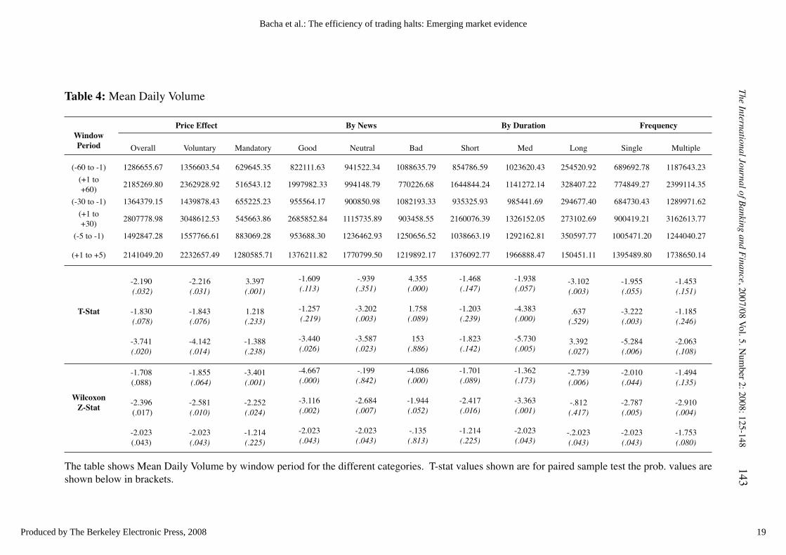
4.6 Effect on Trading VolumeLee et. al., (1994), Ferris et. al. (1992), and Christie et. al. (2002) had all shown similar findings with regards to volume and volatility. All three studies had shown a higher than normal volume and volatility in the pre-suspension period with the trend continuing in the immediate post-suspension period. Where volume is concerned, our results appear to be very much inline with these U.S. based studies. Figure 3 shows the Mean Daily Volume for our overall sample and voluntary/mandatory categories for the 120-day period surrounding halt announcements. There is a clear build-up in daily volume in the period immediately before the halt announcement. The uptrend continues in the period immediately following trading resumption. In all three cases, the rise in traded volume is short lived. It peaks at about 5 days after resumption before sliding steadily back to normal levels. In fact, all the action appears concentrated between days -20 and +20. This is identical to Ferris et. al. (1992) who had reported that volume levels returned to normal 20 days after suspension.

Results of our statistical tests for volume are shown in Table 4. For the overall sample, mean volumes are higher for all 3 post-halt windows; however, the significance tests are mixed. For the sample of 263 voluntary halts, volume is significantly higher (post-halt) in the 5 and 60-day windows. This is in stark contrast to the sample of mandatory halts. Volume, though higher for the +5 day window, is lower for both +30 and +60 day windows. Both the t-test and Wilcoxon show a significantly lower volume for post 60 days relative to 60 days, pre-halt. When we examined volume patterns by news category, though all three categories show higher volume for the +5 day window, in contrast to good and neutral news, the bad news category showed a significantly lower volume for the +60 day window.

9 MCARs for the bad news category is negative for the first 10 day window, but turns marginally positive for the final 10 days.

17







https://www.researchgate.net/publication/4769188_Nasdaq_Trading_Halts_The_Impact_of_Market_Mechanisms_on_Prices_Trading_Activity_and_Execution_Costs?el=1_x_8&enrichId=rgreq-4c3d2692bf46ee8dcae2236e4d8dd616-XXX&enrichSource=Y292ZXJQYWdlOzQxNDU4OTg5O0FTOjE1NDE4NTM2NjUxMTYyM0AxNDEzNzcyMDY0NjY0


Figure 3: Mean Daily Volume for Overall, Voluntary and Mandatory Halts

When examining volume by duration of halt, short duration halts had no different volume in all 3 post-halt windows. Halts of medium duration showed a significantly higher volume in the +5 and +30 windows. Both tests confirmed this at the 5% level. This is interesting since it lends support to the argument that halts will lead to pent-up demand, and therefore, longer duration halts should see a bigger build-up in demand. Indeed, this is true when we go from short to medium duration halts. However, our results for long duration halts are not consistent with this argument. Volume is in fact significantly lower for the +5 and +60 day windows. We believe this could be due to the same argument we had made in explaining the negative CARs for long duration halts. Implying that a long duration halt was needed for a stock signifies more complicated problems; hence, the negative CARs and significantly lower trading volumes.

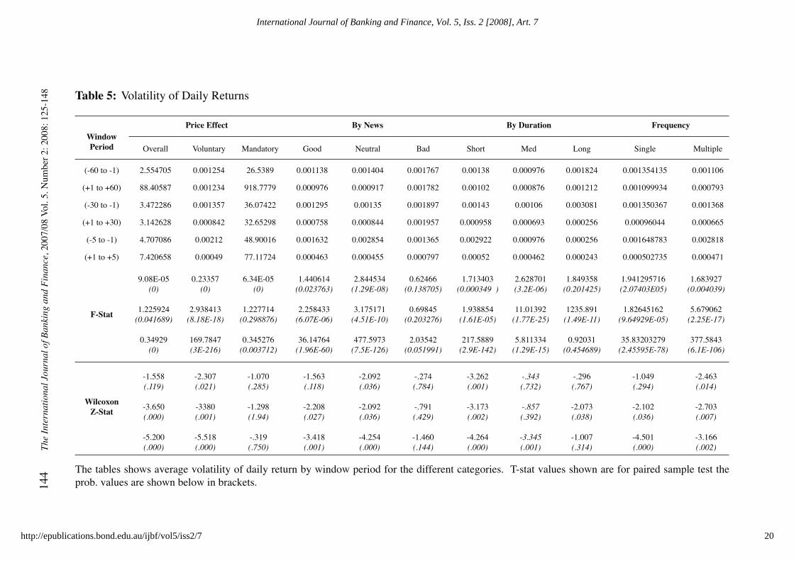
4.7 Impact on VolatilityOur analysis of the impact of halts on returns volatility showed interesting results. Recall that we measure volatility as the variance of daily returns. Table 5 shows the results of our F-test and the non-parametric, Wilcoxon test on the variance of daily returns. Figures 4 and 5 show the plot of daily returns over the 120-day period. Turning to Table 5, variance of returns for the overall sample is significantly higher for all 3 post-halt windows. Post-halt volatility increases as the window period is lengthened. This overall picture changes drastically when we decompose the sample by category.

There is a marked contrast in the post-halt behavior of returns volatility between mandatory and voluntary halts. The mandatory sample has a much higher volatility relative to the voluntary sample, even before halts. This volatility increases very substantially after trading resumes for the mandatory sample. As is obvious from the table, post-halt volatility is sharply higher in the +5 day window than abates,

0

500 000

1000000

1500000

2000000

2500000

3000000

-80 -60 -40 -20 0 20 40 60 80

Days

Volume OVERA LL

VOLUNTARY

MANDATORY

18



The International Journal of B

anking and Finance, 2007/08 V

ol. 5. Num

ber 2: 2008: 125-148

143

Table 4: Mean Daily Volume

Window Period



(-60 to -1) 1286655.67 1356603.54 629645.35 822111.63 941522.34 1088635.79 854786.59 1023620.43 254520.92 689692.78 1187643.23

(+1 to +60)

2185269.80 2362928.92 516543.12 1997982.33 994148.79 770226.68 1644844.24 1141272.14 328407.22 774849.27 2399114.35

(-30 to -1) 1364379.15 1439878.43 655225.23 955564.17 900850.98 1082193.33 935325.93 985441.69 294677.40 684730.43 1289971.62

(+1 to +30)

2807778.98 3048612.53 545663.86 2685852.84 1115735.89 903458.55 2160076.39 1326152.05 273102.69 900419.21 3162613.77

(-5 to -1) 1492847.28 1557766.61 883069.28 953688.30 1236462.93 1250656.52 1038663.19 1292162.81 350597.77 1005471.20 1244040.27

(+1 to +5) 2141049.20 2232657.49 1280585.71 1376211.82 1770799.50 1219892.17 1376092.77 1966888.47 150451.11 1395489.80 1738650.14

T-Stat

-2.190 (.032)

-1.830 (.078)

-3.741 (.020)

-2.216 (.031)

-1.843 (.076)

-4.142 (.014)

3.397 (.001)

1.218 (.233)

-1.388 (.238)

-1.609 (.113)

-1.257 (.219)

-3.440(.026)

-.939 (.351)

-3.202 (.003)

-3.587 (.023)

4.355(.000)

1.758(.089)

153(.886)

-1.468(.147)

-1.203(.239)

-1.823(.142)

-1.938(.057)

-4.383(.000)

-5.730(.005)

-3.102(.003)

.637(.529)

3.392(.027)

-1.955(.055)

-3.222(.003)

-5.284(.006)

-1.453(.151)

-1.185(.246)

-2.063(.108)

Wilcoxon Z-Stat

-1.708 (.088)

-2.396 (.017)

-2.023 (.043)

-1.855 (.064)

-2.581 (.010)

-2.023 (.043)

-3.401(.001)

-2.252(.024)

-1.214(.225)

-4.667(.000)

-3.116(.002)

-2.023(.043)

-.199(.842)

-2.684(.007)

-2.023(.043)

-4.086(.000)

-1.944(.052)

-.135(.813)

-1.701(.089)

-2.417(.016)

-1.214(.225)

-1.362(.173)

-3.363(.001)

-2.023(.043)

-2.739(.006)

-.812(.417)

-.2.023(.043)

-2.010(.044)

-2.787(.005)

-2.023(.043)

-1.494(.135)

-2.910(.004)

-1.753(.080)

The table shows Mean Daily Volume by window period for the different categories. T-stat values shown are for paired sample test the prob. values are shown below in brackets.

19



144

T

he I

nter

nati

onal

Jou

rnal

of B

anki

ng a

nd F

inan

ce, 2

007/

08 V

ol. 5

. Num

ber

2: 2

008:

125

-148 Table 5: Volatility of Daily Returns

Window Period



(-60 to -1) 2.554705 0.001254 26.5389 0.001138 0.001404 0.001767 0.00138 0.000976 0.001824 0.001354135 0.001106

(+1 to +60) 88.40587 0.001234 918.7779 0.000976 0.000917 0.001782 0.00102 0.000876 0.001212 0.001099934 0.000793

(-30 to -1) 3.472286 0.001357 36.07422 0.001295 0.00135 0.001897 0.00143 0.00106 0.003081 0.001350367 0.001368

(+1 to +30) 3.142628 0.000842 32.65298 0.000758 0.000844 0.001957 0.000958 0.000693 0.000256 0.00096044 0.000665

(-5 to -1) 4.707086 0.00212 48.90016 0.001632 0.002854 0.001365 0.002922 0.000976 0.000256 0.001648783 0.002818

(+1 to +5) 7.420658 0.00049 77.11724 0.000463 0.000455 0.000797 0.00052 0.000462 0.000243 0.000502735 0.000471

F-Stat

9.08E-05(0)

1.225924(0.041689)

0.34929(0)

0.23357(0)

2.938413(8.18E-18)

169.7847(3E-216)

6.34E-05(0)

1.227714(0.298876)

0.345276(0.003712)

1.440614(0.023763)

2.258433(6.07E-06)

36.14764(1.96E-60)

2.844534(1.29E-08)

3.175171(4.51E-10)

477.5973(7.5E-126)

0.62466(0.138705)

0.69845(0.203276)

2.03542(0.051991)

1.713403(0.000349 )

1.938854(1.61E-05)

217.5889(2.9E-142)

2.628701(3.2E-06)

11.01392(1.77E-25)

5.811334(1.29E-15)

1.849358(0.201425)

1235.891(1.49E-11)

0.92031(0.454689)

1.941295716(2.07403E05)

1.82645162(9.64929E-05)

35.83203279(2.45595E-78)

1.683927(0.004039)

5.679062(2.25E-17)

377.5843(6.1E-106)

Wilcoxon Z-Stat

-1.558(.119)

-3.650(.000)

-5.200(.000)

-2.307(.021)

-3380(.001)

-5.518(.000)

-1.070(.285)

-1.298(1.94)

-.319(.750)

-1.563(.118)

-2.208(.027)

-3.418(.001)

-2.092(.036)

-2.092(.036)

-4.254(.000)

-.274(.784)

-.791(.429)

-1.460(.144)

-3.262(.001)

-3.173(.002)

-4.264(.000)

-.343(.732)

-.857(.392)

-3.345(.001)

-.296(.767)

-2.073(.038)

-1.007(.314)

-1.049(.294)

-2.102(.036)

-4.501(.000)

-2.463(.014)

-2.703(.007)

-3.166(.002)

The tables shows average volatility of daily return by window period for the different categories. T-stat values shown are for paired sample test the prob. values are shown below in brackets.

20




and is marginally lower for the +30 day window. For the 60-day window, post-halt volatility is several times higher.

While one would expect higher volatility as the sample period is lengthened, the increase in variance is very high for the 60-day windows. 10 In stark contrast to these results, the sample of voluntary halts showed a significantly lower volatility, post-halt. Volatility falls substantially in the +5 day window before rising steadily as the window period lengthens. In fact, as opposed to the mandatory sample, volatility is several fold lower for the 5 and 30-day windows, post-halt.

Figure 4, which shows a scaled plot of daily returns, captures this vast difference in volatility behavior between the two samples11. When we tried to explore the reasons for the very high volatility of the mandatory sample, we came up with 4 possible explanations. Firstly, stocks of companies subjected to mandatory halts (being troubled companies to begin with), had been severely beaten down from their original IPO and par values. Only about half of the sample was selling for above one ringgit, a typical par value. Many selling below 50 sen were essentially “penny stocks”. So, one key reason for the high volatility is the very low traded price. Small, absolute prices lead to large variance.

Figure 4: Volatility of Daily Returns (Scaled), Voluntary vs Mandatory

Secondly, mandatory halts experienced much longer suspensions. The average length of trading suspension for our mandatory sample was 42 days. Howe and Schlarboum (1986) had shown longer suspensions to coincide with bigger, negative residuals. Thirdly, the low liquidity of these stocks might have been a factor, being that low liquidity tends to go hand-in-hand with high volatility. Lastly, probably the

10 This appears to be the instance where the parametric and non-parametric tests produced inconsistent results.11 Daily returns of the mandatory sample were scaled by 10.

-0.4

-0.3

-0.2

-0.1

0

0.1

0.2

0.3

0.4

0.5

-80 -60 -40 -20 0 20 40 60 80

Days

Volatility VOLUNTARY

MANDATORY

21




most important reason for the very high post-halt volatility is information released during suspension. As mentioned earlier, companies subjected to mandatory halts have to come up with viable restructuring plans before trading is allowed to be resumed. We believe the announcement of these plans, which are extensive by nature, leads to an increased uncertainty, especially when initially implemented. Thus, the increased post-halt volatility.

Our results of higher volatility for mandatory halts in the post suspension period are in-line with those findings of Ferris, et. al. (1992) who had examined SEC ordered trading halts. There is also conformity with the results of Wu (1998) who had examined the mandatory halts in Hong Kong. Further, as reported in Wu (1998), the largest change in value is typically on the 1st day of the resumption of trading. This too was consistent in our case. Price variance on day 1 for our mandatory sample was 180%! In fact, price reaction was highest on day 1 for most of our categories. However, our findings of significantly lower volatility for voluntary halts are contradictory to Wu (1998), who had found volatility to be higher post-suspension, even though they were lower than that of the mandatory sample.

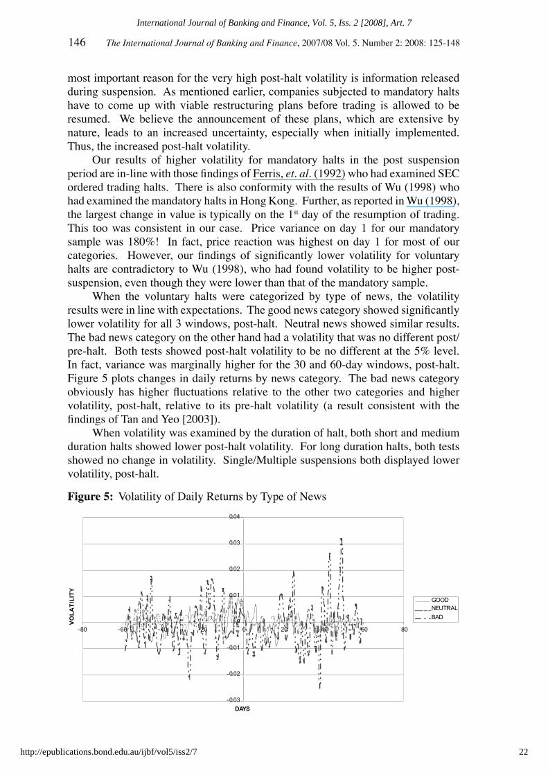
When the voluntary halts were categorized by type of news, the volatility results were in line with expectations. The good news category showed significantly lower volatility for all 3 windows, post-halt. Neutral news showed similar results. The bad news category on the other hand had a volatility that was no different post/pre-halt. Both tests showed post-halt volatility to be no different at the 5% level. In fact, variance was marginally higher for the 30 and 60-day windows, post-halt. Figure 5 plots changes in daily returns by news category. The bad news category obviously has higher fluctuations relative to the other two categories and higher volatility, post-halt, relative to its pre-halt volatility (a result consistent with the findings of Tan and Yeo [2003]).

When volatility was examined by the duration of halt, both short and medium duration halts showed lower post-halt volatility. For long duration halts, both tests showed no change in volatility. Single/Multiple suspensions both displayed lower volatility, post-halt.

Figure 5: Volatility of Daily Returns by Type of News

-0.03

-0.02

-0.01

0

0.01

0.02

0.03

0.04

-80 -60 -40 -20 0 20 40 60 80

DAYS

VOLATILITY

GOODNEUTRAL

BAD

22




https://www.researchgate.net/publication/4991237_Market_Reactions_to_the_Hong_Kong_Trading_Suspensions_Mandatory_versus_Voluntary?el=1_x_8&enrichId=rgreq-4c3d2692bf46ee8dcae2236e4d8dd616-XXX&enrichSource=Y292ZXJQYWdlOzQxNDU4OTg5O0FTOjE1NDE4NTM2NjUxMTYyM0AxNDEzNzcyMDY0NjY0


5. Conclusion

Most of our findings were broadly consistent and logical. Trading halts are indeed significant events, with the type of halt (whether voluntary or mandatory) mattering tremendously. The type of news released during the halt is the critical determinant of how price, volume, and volatility would behave, post-halt. Also, the duration of halt and frequency, whether single or multiple, appears to be largely inconsequential, while anticipatory behavior/information leakages appear to go hand-in-hand with trading halts.

Our results support the price efficiency hypothesis of trading halts. Mandatory halts and the ‘bad news’ category had shown an increased volatility and reduced trading volume, thereby lending support to the “learning through trading argument”. With the exception of these two subsets, our overall results are consistent with the argument that trading halts help disseminate information, thus enhancing the price discovery process.

Trading halts had resulted in a positive price reaction, increased volume, and volatility. There was indeed a significant difference in the results of voluntary as opposed to mandatory halts. The type of news released during the halt had a huge impact on all three variables of price, volume, and volatility, post-halt. The duration of halt had an isolated impact and appears to be largely inconsequential. The frequency of halts, whether single or multiple, did not seem to matter either.

Comparing our results with that of previous studies, we found that for all three variables examined, there was broad conformity concerning our overall sample. However, when we refined the analysis by examining the sub categories, we found some interesting differences. We found significantly positive CARs, post-halt, for our sample of mandatory halts, along with significantly lower volatility, post halt, for the voluntary sample.

Author statement: Obiyathulla I. Bacha, Mohamed E. S. Abdul Rashid and Roslily Ramlee are staff members of the International Islamic University Malaysia. The authors acknowledge with thanks the financial support provided by the Research Centre at the IIUM. E-mail: [email protected]

References

Bhattacharya, U., and M. Spiegel (1998). Anatomy of a Market Failure; NYSE Trading

Suspensions (1974 – 1988), Journal of Business & Economic Statistics April, 216 – 226.

Chen, H., H. Chen and N. Valerios (2003) The effects of trading halts on price discovery for NYSE stocks, Applied Economics 35: 91 – 97.

Christie, W.G., S.A. Corwin, and J.H. Harris, (2002). Nasdaq Trading Halts: The Impact of Market Mechanisms on Prices, Trading Activity, and Execution Costs, The Journal of Finance LVII(3): 1443 – 1478.

23







Duque, J., and A.R. Fazenda (2003). Evaluating market supervision through an overview of trading halts in the Portuguese stock market, Journal of Financial Regulation and Compliance 11(4): 349 – 376.

Ferris, S.P., R. Kumar and G.A. Wolfe (1992) The Effect of SEC – Ordered Suspensions on Returns, Volatility and Trading Volume, The Financial Review 27(1): 1 – 34.

Hopewell, M.H., and A.L. Schwartz (1978). Temporary Trading Suspensions In Individual NYSE Securities, The Journal of Finance 33(5): 1355 – 1373.

Howe, J. S., and G.G. Schlarbaum (1986). SEC Trading Suspensions: Empirical Evidence, Journal of Financial and Quantitative Analysis 21(3): 323 – 333.

Kabir, R., (1994). Share price behaviour around trading suspensions on the London Stock Exchange, Applied Financial Economics 24: 289 – 295.

Lee, M.C., M. J. Ready and P.J. Seguin (1994). Volume, Volatility, and New York Stock Exchange Trading Halts, The Journal of Finance XLIX(1): 183 – 211.

McDonald, C.G., and D. Michayluk (2003). Suspicious trading halts, Journal of Multinational Financial Management 13: 251 – 263.

Tan, S.K., and W.Y. Yeo (2003). Voluntary Trading Suspension in Singapore, Applied Financial Economics 13: 517 – 523.

Wu, L., (1998). Market Reactions to the Hong Kong Trading Suspensions: Mandatory versus Voluntary, Journal of Business Finance & Accounting 25(3 & 4): 419 – 437.

24






https://www.researchgate.net/publication/24071339_Share_Price_Behaviour_Around_Trading_Suspensions_on_the_London_Stock_Exchange?el=1_x_8&enrichId=rgreq-4c3d2692bf46ee8dcae2236e4d8dd616-XXX&enrichSource=Y292ZXJQYWdlOzQxNDU4OTg5O0FTOjE1NDE4NTM2NjUxMTYyM0AxNDEzNzcyMDY0NjY0

https://www.researchgate.net/publication/24071339_Share_Price_Behaviour_Around_Trading_Suspensions_on_the_London_Stock_Exchange?el=1_x_8&enrichId=rgreq-4c3d2692bf46ee8dcae2236e4d8dd616-XXX&enrichSource=Y292ZXJQYWdlOzQxNDU4OTg5O0FTOjE1NDE4NTM2NjUxMTYyM0AxNDEzNzcyMDY0NjY0

https://www.researchgate.net/publication/227406024_SEC_Trading_Suspensions_Empirical_Evidence?el=1_x_8&enrichId=rgreq-4c3d2692bf46ee8dcae2236e4d8dd616-XXX&enrichSource=Y292ZXJQYWdlOzQxNDU4OTg5O0FTOjE1NDE4NTM2NjUxMTYyM0AxNDEzNzcyMDY0NjY0

https://www.researchgate.net/publication/227406024_SEC_Trading_Suspensions_Empirical_Evidence?el=1_x_8&enrichId=rgreq-4c3d2692bf46ee8dcae2236e4d8dd616-XXX&enrichSource=Y292ZXJQYWdlOzQxNDU4OTg5O0FTOjE1NDE4NTM2NjUxMTYyM0AxNDEzNzcyMDY0NjY0

https://www.researchgate.net/publication/4737483_Temporary_Trading_Suspensions_in_Individual_NYSE_Securities?el=1_x_8&enrichId=rgreq-4c3d2692bf46ee8dcae2236e4d8dd616-XXX&enrichSource=Y292ZXJQYWdlOzQxNDU4OTg5O0FTOjE1NDE4NTM2NjUxMTYyM0AxNDEzNzcyMDY0NjY0

https://www.researchgate.net/publication/4737483_Temporary_Trading_Suspensions_in_Individual_NYSE_Securities?el=1_x_8&enrichId=rgreq-4c3d2692bf46ee8dcae2236e4d8dd616-XXX&enrichSource=Y292ZXJQYWdlOzQxNDU4OTg5O0FTOjE1NDE4NTM2NjUxMTYyM0AxNDEzNzcyMDY0NjY0









https://www.researchgate.net/publication/223044669_Suspicious_trading_halts?el=1_x_8&enrichId=rgreq-4c3d2692bf46ee8dcae2236e4d8dd616-XXX&enrichSource=Y292ZXJQYWdlOzQxNDU4OTg5O0FTOjE1NDE4NTM2NjUxMTYyM0AxNDEzNzcyMDY0NjY0

https://www.researchgate.net/publication/223044669_Suspicious_trading_halts?el=1_x_8&enrichId=rgreq-4c3d2692bf46ee8dcae2236e4d8dd616-XXX&enrichSource=Y292ZXJQYWdlOzQxNDU4OTg5O0FTOjE1NDE4NTM2NjUxMTYyM0AxNDEzNzcyMDY0NjY0

https://www.researchgate.net/publication/228254233_Evaluating_Market_Supervision_Through_an_Overview_of_Trading-Halt_in_the_Portuguese_Stock_Market?el=1_x_8&enrichId=rgreq-4c3d2692bf46ee8dcae2236e4d8dd616-XXX&enrichSource=Y292ZXJQYWdlOzQxNDU4OTg5O0FTOjE1NDE4NTM2NjUxMTYyM0AxNDEzNzcyMDY0NjY0



The efficiency of trading halts: Emerging market evidence

Documents

Transcript of The efficiency of trading halts: Emerging market evidence