The Effects of Rural Electrification on Employment: New Evidence from South Africa

Taryn Dinkelman

Web Appendix

Web Appendix 1: Data description, variable construction and sample selection

This appendix describes all of the data sources used in the paper.

1 Census data

Census community data 1996 and 2001: 100% sample obtained from Statistics South Africa.

Census is adjusted for undercount after enumeration.1. Data are provided at an aggregated

enumeration area level in 1996 and at an aggregated sub-place level in 2001.

Variables in the Census include: counts of employment, population, levels of educational

attainment and recent in-migrant status by sex, race and age group; counts of households,

female-headed households, and households living below a poverty line (demarcated by annual

household income of ZAR 6,000 or less); counts of households using different sources of fuel

for lighting and counts of households with access to different types of water and sanitation

facilities. Statistics South Africa also provided me with counts of households using different

fuels for cooking at the enumeration area (1996) and sub-place level (2001). A limited set of

cross-tabulated variable counts are also available in these data.

Employment variables in the Census: As in most Census data, measures of employment are

broad. In 1996, adults are asked: ‘Does the person work?’ Activities listed as work include

formal work for a salary or wage, informal work such as making things for sale or selling

things or rendering a service, work on a farm or the land, whether for a wage or as part

of the household’s farming activities. I define everyone answering yes to this question as

employed, else not employed.

In 2001, adults were asked: ‘Did the person do any work for pay, profit or family gain

for one hour or more?’ Possible responses were: yes (formal, registered, non-farming), yes

(informal, unregistered, non-farming), yes (farming) and no (did not have work). Everyone

who answers yes to this question is defined as employed, else not employed.

1Personal Communication with Piet Alberts, Senior Statistician in the Census department of StatisticsSouth Africa, May 2007

1

Questions about employment are similar across Census waves, although the 2001 em-

ployment definition is somewhat broader than the 1996 variable, describing individuals who

work for even one hour per week as employed. Since the main outcome variable is the change

in employment rate, these differences will only be problematic if reported part-time work

differentially contributes to new employment with lower gradient.

Creating the Census panel of communities: The 2001 Census geography is hierarchically or-

dered as follows, from largest to smallest unit:

• District: represents a local labor market area in KwaZulu-Natal, containing between

30,000 and 50,000 households.

• Main place or sub-districts: correspond to groupings of towns and surrounding areas.

• Community or sub-places: the lowest unit of observation in the 2001 Census data.

Average community size is small: between 200 and 250 households on average.

Boundaries for communities from the 2001 Census define the main unit of analysis. I ag-

gregate the 1996 (smaller) areas up to the (larger) 2001 boundaries.2 The matched identifiers

from this panel of areas are used to extract Census aggregate data in 1996 and 2001. For

each 1996 EA, the proportion of the EA polygon area that falls inside each 2001 community

is calculated. This proportion is used as a weight to assign a proportion of the 1996 EA data

to the 2001 community. The key assumption in this process is that people are uniformly

distributed over 1996 EA’s.

Selection of communities for sample: Within the set of 4,030 communities in KwaZulu Natal,

I restricted the sample to include rural, tribal areas. Communities that were defined as

national parks and mines were also excluded. This left 1,992 communities. A final exclusion

of communities with fewer than 100 adults in either Census year reduced the sample further

by 176 communities, leaving 1,816 in the final analysis sub-sample.

2 Household Surveys: 1995, 1997, 1999, 2001

Obtained from Statistics South Africa. Four waves of household survey data (October House-

hold Surveys for the 1990s and the September Labor Force Survey in 2001) resembling the

2Statistics South Africa notes that EA boundaries should never cut across existing administrative bound-aries, and all “social boundaries should be respected” (StatsSA, 2000). However, boundaries have shiftedover time (Christopher, 2001). In most cases, re-demarcation involved the following real changes to 1996EA’s: “splits” that occurred when obstacles or boundaries divided the EA naturally, and “merges” that oc-curred between EA’s that were small or that were legally, socially or naturally a geographical entity. Changeswere made only when “absolutely necessary” (StatsSA, 2000: 21, 26).

2

World Bank LSMS surveys. Each wave is a nationally representative sample of individuals.

The lowest level of geography that can be identified in these household surveys is the Mag-

isterial District, of which there are 38 in rural KZN. I include all Magisterial Districts in the

analysis.

Selection of individuals for inclusion in sample: I use the sample of African male and female

adults (ages 15-59) living in rural KwaZulu-Natal who report information about employment

as well as about hours of work and total monthly earnings. I compute hourly wages using

monthly earnings and usual hours of work reports.

3 Schools Register of Needs 1995 and 2000

These data are provided by the South African Department of Education for schools in 1995

and 2000. GPS coordinates for each school are used to assign schools to Census community

boundaries. Each community is assigned the total number of schools in each year as well as

the change in the total number of schools over the five-year period.

4 Geographic data

Land gradient: The source for these data is the 90-meter Shuttle Radar Topography Mission

(SRTM) Global Digital Elevation Model available at www.landcover.org. Digital elevation

model data was used to construct measures of average land gradient for each Census com-

munity using GIS software (ArcMap 9.1). Gradient is measured in degrees from 0 (perfectly

flat) to 90 degrees (perfectly vertical). The distribution of land gradient in my sample area

is shown in Web Appendix 1 Figure 1.

Other measures of proximity: Spatial data on Eskom’s 1996 grid network (high and medium

voltage lines and substations) was provided by Steven Tait at Eskom. These data were

used to calculate straight line distances between Census centroids and the nearest electricity

substation.

Census 1996 spatial data were used to generate straight line distances from each commu-

nity centroid to the nearest road and town in 1996.

Census 2001 spatial data were used to create measures of the area of the sub-place. I used

these area measures in conjunction with total household counts from the Census community

data to create household density variables in 1996 and 2001.

3

5 Electricity project data

Data on Eskom projects in KwaZulu-Natal were provided by Sheila Brown at Eskom. The

project list gives the number of pre-paid electricity connections per Eskom-defined area in

each year from 1990 to 2007. I define the year of electrification as the year in which a

community experienced a spike in household connections (concentrated project activity).

Areas are referenced by name and village code. Eskom’s planning units do not line up

accurately with Census regions. To match project data to Census regions, I map the project

data to a physical location using a spatial database of transformer codes linked to project

codes and then merge these locations to Census boundaries. Areas designated as Eskom

project and non-project areas are displayed in Web Appendix 1 Figure 2.

References

Africa, Statistics South, “Census Mapping Manual,” Technical Report, Statistics South

Africa http : //www.statssa.gov.za/africagis2005/presentations/oralcolemandube.pdf

2000.

Christopher, A.J., The Geography of Apartheid, Johannesburg: Witwatersrand

University Press, 2001.

4

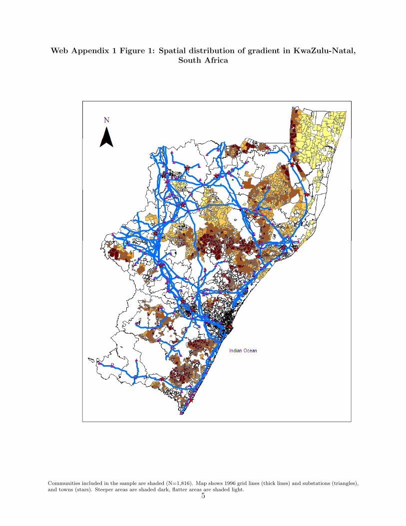
Web Appendix 1 Figure 1: Spatial distribution of gradient in KwaZulu-Natal,South Africa

Communities included in the sample are shaded (N=1,816). Map shows 1996 grid lines (thick lines) and substations (triangles),and towns (stars). Steeper areas are shaded dark, flatter areas are shaded light.

5

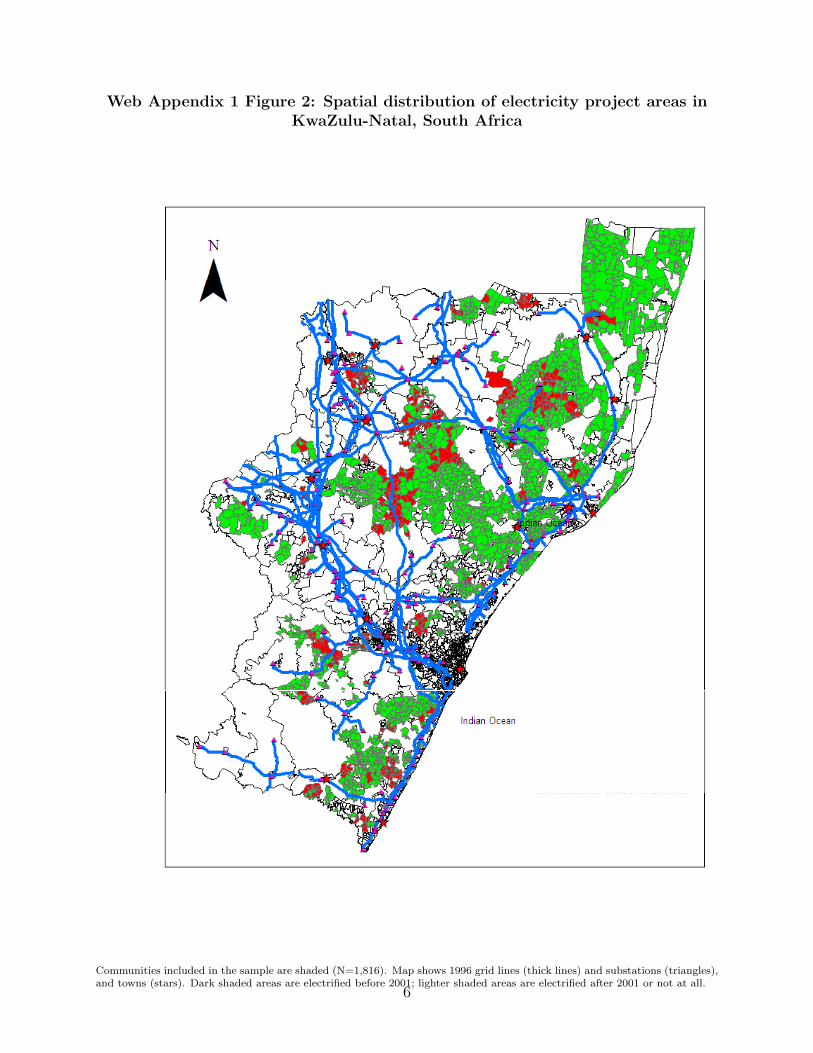
Web Appendix 1 Figure 2: Spatial distribution of electricity project areas inKwaZulu-Natal, South Africa

Communities included in the sample are shaded (N=1,816). Map shows 1996 grid lines (thick lines) and substations (triangles),and towns (stars). Dark shaded areas are electrified before 2001; lighter shaded areas are electrified after 2001 or not at all.

6

Web Appendix 2: Heterogeneity in electrification effects

In this appendix, I explore the characteristics of communities that contribute the most to

the main employment results from the IV strategy.

1 Heterogeneous effects related to income

As part of the South African electrification, once an area had been targeted for new access,

each household received a basic connection package: an electric circuit board, a pre-payment

meter, three plug points and one light bulb. Households received a default supply of 2.5

amperes or could upgrade to a 20 ampere supply for a fee of about ZAR40 (USD6.00), which

most of Eskom’s 3 million customers chose to do (Gaunt, 2003). Although industry experts

agreed that “Electric lighting was synonymous with the roll-out”, and that the NEP did

reach poor households, the subsidized roll-out really changed the option to use electricity.

Households were still required to pay for using the service by purchasing electricity credits

loaded on to pre-paid cards. In 1999, household electricity cost $0.039 per kilowatt hour

(kWh). Estimates of load demand from Eskom reports suggest that most rural households

used between 35 and 60 kWh per month, translating into energy expenses of between $1.37

and $2.34 per month (Gaunt, 2003), or 1.8 percent of median monthly household income in

rural KZN in 1995. Because of this positive marginal cost, the poorest households are likely

to have been the least responsive to the new technology in the short-run.

The main IV strategy used in the paper identifies employment effects for communities

that are cheaper to electrify by virtue of having a flatter gradient. As is well known, the IV

coefficient is a weighted sum of effects for different groups, each of which may be differently

affected by the gradient instrument (Kling, 2001). If different groups also experience a

different electrification effect, then the IV result will be driven by the groups that are weighted

most heavily in the IV parameter estimate. These weights determine which group’s effect

contributes the most to the total measured effect in the IV regressions.

In communities with flatter gradient, female employment may be more responsive to

electrification than in an average newly electrified community. One way in which marginal

communities could differ from average communities is in their ability to switch home produc-

tion technologies when the new service arrives. In creating the IV weights below, I investigate

how much of the IV coefficient is driven by changes in communities that look as if they would

be in a better position to switch to using electricity once the new connections are made. Us-

ing electricity more effectively involves buying complementary appliances so this requires

focusing on heterogeneous effects of electrification by some measure of household income.

Since the Census provides only a crude measure of poverty (household income is reported

1

in intervals not consistent over time), I combine the three poverty indicators into a poverty

index and consider the characteristics of communities in each quintile of this index. To

create the index, I follow Card (1995) and Kling (2001): for the sample of communities in

the steepest half of the gradient distribution, I use a logit model to estimate the probability

of receiving an electricity project using the baseline poverty rate, the baseline female/male

sex ratio and the baseline share of female-headed households. Using coefficients from this

regression, a value for every community in the sample is predicted. Each community is then

assigned to a quintile of the predicted poverty index, where quintile cut-points are defined

on the estimation sample only.

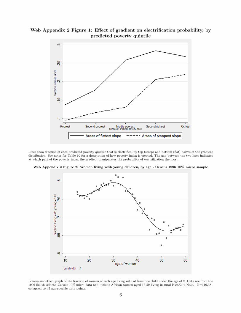
The graph in Web Appendix 2 Figure 1 shows the fraction of communities in each pre-

dicted poverty quintile that is electrified between 1996 and 2001, separately for communities

in the flattest and steepest halves of the gradient distribution. Both lines slope upwards, indi-

cating that areas with higher predicted values of the poverty index (i.e. richer areas) are more

likely to receive an electricity project at all. The gap between the two lines shows that flatter

areas are systematically more likely to be electrified than steeper areas. The middle-poorest

and second-richest quintiles are most likely to have the probability of a project manipulated

by the instrument, which can be seen in the larger gap between the lines occurring at these

quintiles.

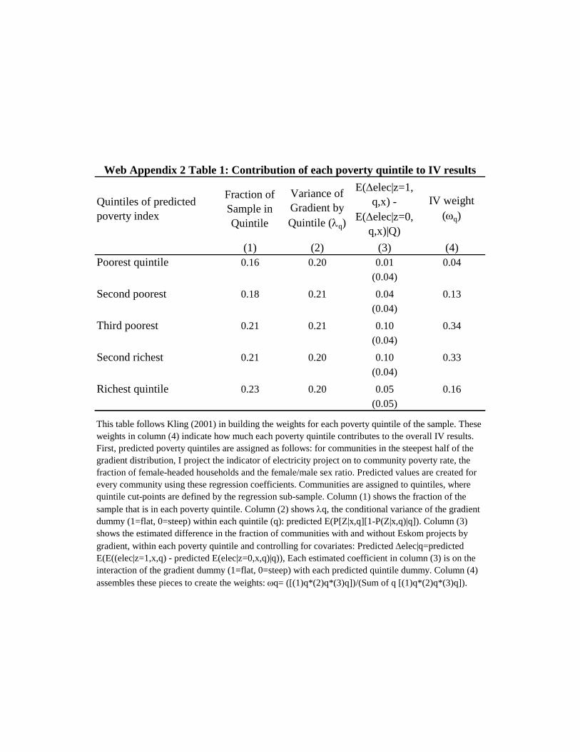
Some of the same information is provided in Web Appendix 2 Table 1. This table builds

up the IV weights for each poverty quintile of the sample. The fraction of the sample

falling within each predicted poverty quintile is presented in column (1); the variance of

gradient across communities within each quintile is very similar across quintiles, as column

(2) indicates. Column (3) echoes Web Appendix 2 Figure 1: there is a larger difference in

the fraction of communities electrified across flat and steep areas, in the third poorest and

second richest quintiles. In column (4) of that table, I compute the contribution of each

quintile to the final IV estimate by calculating the relevant weight (explained in the table

notes): we see from the results that middle quintile and the second richest quintile together

contribute over 65 percent to the IV result.

Middle quintiles in particular may have larger employment effects because they contain

households that experience larger changes in home production technology when electricity

arrives compared to richer quintiles, and they are more able to effectively use the new

technology than the poorest quintiles. Web Appendix 2 Table 2 shows that middle-poor

areas are initially less likely to be using electricity than richer areas and are more reliant on

wood for cooking (columns 1 to 3). Columns (4), (5) and (6) of this table present within-

quintile reduced-form coefficients from regressions of the change in fuel use on a gradient

dummy (1 is flat, 0 is steep). These columns indicate large increases in the use of electricity

2

and large decreases in reliance on wood for cooking in flatter areas for middle-poor, second-

richest and richest areas.1 Finally, column (7) of Web Appendix 2 Table 2 indicates that the

female employment result is indeed driven by women living in middle- and second-richest

quintile communities: the effects for these communities are large, positive and significant

and are weighted most heavily in the final IV results. The coefficients in this table are akin

to reduced-form coefficients from a regression of the outcome variable on a binary version of

the instrument and all controls. Dividing each coefficient by the corresponding coefficient in

column (3) of Web Appendix 2 Table 1 will reproduce the IV coefficient.

2 Heterogeneous effects related to other constraints on women’s time

Women who have home-production responsibilities are less likely to be able to respond to

new access to electricity, even though productivity at home may be substantially enhanced

by the use of electricity. For example, child-care responsibilities raise the value of a woman’s

time at home and in the absence of pre-school care, this value only falls when children

start school. Officially, school-starting age is between ages 6 and 7 in South Africa, but

enrollment only reaches 90% by around age 9 (results from 2001 10% Census micro data,

not shown). Children also create work at home though, and so the more children in the

house that require child-care, the more time can potentially be saved with access to a more

efficient power source. It is therefore not clear whether women with younger children will

supply more or less of their labor to the market, in response to new household electrification.

Census micro data from 1996 give some indication of which women are more likely to live

with a child younger than age 9. Web Appendix 2 Figure 2 is a lowess-smoothed graph of

the fraction of women of each age living with at least one child aged 9 or under. The graph

is drawn for African women between ages 15 and 59 living in rural areas of KZN and shows

a clear distribution of youngest children to households with both younger and older women.2

After age 30 and up to about age 50, the probability of a woman living with a child who

requires constant care falls substantially.

To investigate whether the employment effects of household electrification are largest for

this latter group of women, I redefine the outcome variable to be yajdt =Eajdt

Pjdt, where Eajdt is

the number of employed women in age group a for each of nine five-year cohorts and Pjdt is the

total adult female population in each community in each year. This definition decomposes

the employment result into effects for each age cohort: the estimated coefficients sum to

1This is related to the point by Greenwood et al (2005) who argue that poorer households are the last toadopt durable goods for home production.

2The allocation of young children to households with older women is a common pattern in South Africa,where pension-aged women care for grandchildren in skip-generation households (Case and Deaton, 1998).

3

the main electrification coefficient in the final column of Table 4 in the main paper. Web

Appendix 2 Table 3 presents OLS and IV coefficients (and robust standard errors clustered

at the sub-district level) on the electrification dummy for separate regressions.3 IV results

are large and positive for each age group, but significant only for women in their thirties and

late forties. Employment grows by 3 percentage points for women between the ages of 30

and 34, by 1.7 percentage points for the 35 to 39 year old group and by a smaller but still

significant 1.4 percentage points for women in their late forties. Together, these age groups

account for 65 percent of the total female employment result. This indicates that women in

age groups in which care of young children is not a significant constraint, are those women

most responsive to the arrival of electricity in the home.

3Results for men are not shown as the electrification coefficient was never significant for any cohort.

4

References

Card, David, “Using geographic variation in college proximity to estimate the returns to

schooling,” in L.N. Christofides et al, ed., Aspects of labour market behaviour: Essays in

honor of John Vanderkamp, Toronto: University of Toronto Press, 1995, pp. 201–221.

Case, Anne and Angus Deaton, “Large cash tranfers to the elderly in South Africa,”

Economic Journal, September 1998, 108 (450), 1330–1361.

Gaunt, Trevor, “Electrification technology and processes to meet economic and social

objectives in Southern Africa.” PhD dissertation, University of Cape Town 2003.

Greenwood, Jeremy, Ananth Seshadri, and Mehmet Yorukoglu, “Engines of

Liberation,” Review of Economic Studies, 2005, 72, 109–133.

Kling, Jeffrey, “Intepreting instrumental variables estimates of the returns to schooling,”

Journal of Business and Economic Statistics, July 2001.

5

Web Appendix 2 Figure 1: Effect of gradient on electrification probability, bypredicted poverty quintile

Lines show fraction of each predicted poverty quintile that is electrified, by top (steep) and bottom (flat) halves of the gradientdistribution. See notes for Table 10 for a description of how poverty index is created. The gap between the two lines indicatesat which part of the poverty index the gradient manipulates the probability of electrification the most.

Web Appendix 2 Figure 2: Women living with young children, by age - Census 1996 10% micro sample

Lowess-smoothed graph of the fraction of women of each age living with at least one child under the age of 9. Data are from the1996 South African Census 10% micro data and include African women aged 15-59 living in rural KwaZulu-Natal. N=116,381collapsed to 45 age-specific data points.

6

Quintiles of predicted poverty index

Fraction of Sample in Quintile

Variance of Gradient by Quintile (q)

E(elec|z=1, q,x) -

E(elec|z=0, q,x)|Q)

IV weight (q)

(1) (2) (3) (4)Poorest quintile 0.16 0.20 0.01 0.04

(0.04)

Second poorest 0.18 0.21 0.04 0.13(0.04)

Third poorest 0.21 0.21 0.10 0.34(0.04)

Second richest 0.21 0.20 0.10 0.33(0.04)

Richest quintile 0.23 0.20 0.05 0.16(0.05)

hi bl f ll li ( ) i b ildi h i h f h i il f h l h

Web Appendix 2 Table 1: Contribution of each poverty quintile to IV results

This table follows Kling (2001) in building the weights for each poverty quintile of the sample. These weights in column (4) indicate how much each poverty quintile contributes to the overall IV results. First, predicted poverty quintiles are assigned as follows: for communities in the steepest half of the gradient distribution, I project the indicator of electricity project on to community poverty rate, the fraction of female-headed households and the female/male sex ratio. Predicted values are created for every community using these regression coefficients. Communities are assigned to quintiles, where quintile cut-points are defined by the regression sub-sample. Column (1) shows the fraction of the sample that is in each poverty quintile. Column (2) shows q, the conditional variance of the gradient dummy (1=flat, 0=steep) within each quintile (q): predicted E(P[Z|x,q][1-P(Z|x,q)|q]). Column (3) shows the estimated difference in the fraction of communities with and without Eskom projects by gradient, within each poverty quintile and controlling for covariates: Predicted elec|q=predicted E(E((elec|z=1,x,q) - predicted E(elec|z=0,x,q)|q)), Each estimated coefficient in column (3) is on the interaction of the gradient dummy (1=flat, 0=steep) with each predicted quintile dummy. Column (4) assembles these pieces to create the weights: q= ([(1)q*(2)q*(3)q])/(Sum of q [(1)q*(2)q*(3)q]).

Electric Lighting

Electric Cooking

Wood Cooking

Electric Lighting

Electric Cooking

Wood Cooking Females Males

(1) (2) (3) (4) (5) (6) (7) (8)Poorest quintile 0.02 0.01 0.90 0.00 0.002 0.000 0.001 -0.005

(0.08) (0.05) (0.15) (0.02) (0.01) (0.02) (0.00) (0.01)

Second 0.04 0.02 0.85 0.00 0.004 -0.012 0.00806* 0.001(0.14) (0.08) (0.19) (0.02) (0.01) (0.01) (0.00) (0.01)

Third 0 07 0 03 0 81 0 04 0 0152* 0 0193* 0 00792* 0 002

Fuel Use in Home Production: Fraction using [X] in 1996

Web Appendix 2 Table 2: Household energy use by poverty quintile: At baseline and over time, 1996 to 2001

t in employment by gradient

t in Fuel Use for Home Production: Within-quintile difference by gradient Quintile of

predicted poverty index

Third 0.07 0.03 0.81 0.04 0.0152* -0.0193* 0.00792* 0.002(0.17) (0.10) (0.22) (0.02) (0.01) (0.01) (0.00) (0.01)

Fourth 0.12 0.05 0.72 0.03 0.0214** -0.0337** 0.0101* 0.002(0.23) (0.12) (0.26) (0.02) (0.01) (0.01) (0.01) (0.01)

Richest quintile 0.18 0.09 0.64 0.04 0.0258** -0.025 -0.002 -0.012(0.27) (0.16) (0.30) (0.03) (0.01) (0.02) (0.01) (0.01)

Columns (1)-(3) present the quintile means of outcome variables in 1996, columns (4)-(8) present coefficients from regression of interactions of gradient dummy and predicted poverty quintile. Significant at p<0.01***, p<0.05** or p<0.1* level.

t Female Employment OLS IV(1) (2)

Ages 15-19 0.000 0.000(0.000) (0.005)

Ages 20-24 0.000 0.009(0.001) (0.013)

Ages 25-29 -0.001 0.015(0.001) (0.012)

Ages 30-34 -0.001 0.030*(0.001) (0.012)

Ages 35-39 0.000 0.017(0.001) (0.013)

Ages 40-44 0.001 0.007(0.001) (0.012)

Web Appendix 2 Table 3: Age-specific effects of Electrification on Female Employment

(0.001) (0.012)

Ages 45-49 0.001 0.014*(0.001) (0.008)

Ages 50-54 -0.001 -0.001(0.001) (0.007)

Ages 55-59 0.001 0.004(0.001) (0.006)

Each cell in the table shows the coefficient (standard error) on the Eskom Project indicator from an OLS or IV regression of the change in the age-specific female employment rate on all controls, as in Table 3. Age-specific female employment rate is measured as the fraction of employed African women of age [X] over all females, where [X] is one of nine age groups. Robust standard errors clustered at sub-district level. Significant at p<0.01***, p<0.05** or p<0.1* level. N=1,816 in each regression.

Web Appendix 3: Robustness checks

This appendix provides a set of additional statistical tests and robustness checks for the

paper.

1 Reduced form for second stage estimates

Web Appendix Table 1 presents the coefficients on gradient in the reduced form regressions

of the main outcomes– the change in female employment and change in male employment

rates– on gradient and all other controls. The results show that there is a reduced form

relationship between community land gradient and the change in community-level female

employment; but the reduced form relationship between gradient and male employment

growth is not statistically significant at conventional levels.

2 Controlling for political factors

I collected election outcomes data for the KZN municipalities for the first municipal elections

in 2000 and matched my sample of Census communities (smaller entities) to the municipality

boundaries (larger entities). Using the number of voters voting for each of 9 parties i in each

municipality in the 2000 elections, I create a standard measure of political competition (see

Banerjee and Somanathan, 2007), assigning to each community j the corresponding value of

Hj:

Hj = (1−9∑

i=1

votesharej) (1)

A higher level of Hj indicates more political competition. Results for results, controlling

for political heterogeneity are presented in Web Appendix 3 Table 2 and Table 3.

• Table 2 columns (1) and (2) show that the measure of political competition predicts

whether a community gets an Eskom project, but only when we do not control for

district fixed effects. Once all other controls and district FE are added, the political

competition measure has no predictive power in the first stage. More importantly, its

inclusion does not change the impact of gradient on the probability of being allocated

an Eskom project

• Table 3 columns (1) - (8) show that the inclusion of the political competition vari-

able changes the effects of electrification on female employment only slightly. In areas

with more political competition, female employment grows by 3.8 percentage points

1

(going from no to complete competition). In the IV results, female employment is

higher by 8.9 percentage points but given the reduction in sample size, this coefficient

is not significantly different from zero (not all communities could be mapped to mu-

nicipal boundaries). Male results are not affected by including the control for political

heterogeneity

Although it would be preferable to control for earlier elections outcomes than 2000, this

is not possible since the earlier election was “transitional” and those political boundaries

were in flux before 2000. The exercise here indicates that while political competition may

be important for employment growth, this variable is uncorrelated with gradient after con-

trolling for all other variables and district fixed effects; and so has no substantial effect on

the IV employment growth results.

3 Restricting the sample to areas without roads

I do not have access to road-building data in the province over time; only an indicator for

whether a major national road runs through a community in 1996. In Web Appendix 3

Table 2 and Table 3, I present results from re-estimating the first stage assignment model

and the model for employment on a smaller sample, where I omit communities with a main

road running through them. The results for female employment (Table 2, columns (9) -

(18)) remain large and positive, although, since the sample shrinks with the exclusion of

some communities, the estimate is no longer statistically significant at conventional levels.

The AR confidence interval extends from [0; 0,2].

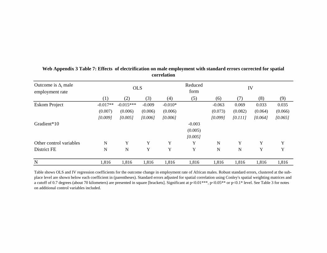
4 Main results with corrections for spatial correlation in unobservables

To check that the main results (both coefficient estimates and statistical significance) are

robust to spatial correlation in the error term, I re-estimate all regression results using the

approach of Conley (1999). Results appear in Web Appendix Tables 4 to 7. In this approach,

standard errors are generated using a weighted estimator, where the weights are the product

of two weight functions, or kernels (one with an East-West orientation and the other with a

North-South orientation). Each kernel declines linearly and is zero beyond a cutoff number.

The cutoff number I choose here is 0.7 degrees (roughly 70 kilometers) and results are robust

to cutoffs from 0.6 degrees to 1 degree (60 kms to 100kms).

Two points are apparent from these tables. For the chosen cutoff values, the coefficient

estimates remain stable. And, standard errors are not uniformly larger when corrected for

spatial correlation: sometimes they are larger and sometimes smaller than standard errors

2

clustered at the sub-district level. The reason for this is that clustering standard errors at

the sub-district level already takes account of most of the spatial correlation in errors.

Overall, the tables show that OLS and IV estimates and inference related to these esti-

mates is robust to this alternative form of computing standard errors.

5 Testing for differences between male and female employment effects

Web Appendix 3 Table 8, I test for differences in the effect of electrification on male and

female employment. I implement the test by differencing male and female outcome variables

within community and then estimating the same set of OLS and IV regressions on this

new variable. This test respects the correlated structure of errors across male and female

regressions. Results indicate we cannot reject that new Eskom Projects had the same impact

on male and female employment growth.

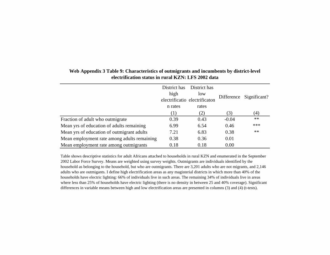
6 Characteristics of outmigrants compared to incumbents across high and low

electrification areas, LFS 2002

The September 2002 Labor Force Survey contains a special module on migrants attached

to households, from which information on outmigrants can be derived. In Web Appendix

3 Table 9, I show the fraction of people who are outmigrants from rural KZN magisterial

districts as measured in these data. The table also presents mean employment rates and

mean years of education for outmigrants and incumbents.

The table show differences in these summary statistics across communities with high and

low rates of electrification (column 3) and indicates whether these differences are statistically

significant (column 4). High electrification areas are defined as any magisterial districts in

which more than 40% of the households have electric lighting: 66 percent of individuals live

in such areas. The remaining 34% of individuals live in areas where less than 25 percent of

households have electric lighting (there is no density in between 25 and 40 percent coverage).

Note that:

• Outmigration rates from rural KZN are high, and significantly higher in areas with low

rates of electrification

• Outmigrants have higher average education than those who remain behind

• Employment rates of either group are about the same across high and low electricity

districts

3

• Employment rates are significantly (significant at the 1% level) higher among incum-

bents compared to outmigrants in both low and high electrification rate districts.

References

Banerjee, Abhijit and Rohini Somanathan, “The political economy of public goods:

Some evidence from India,” Journal of Development Economics, 2007, 82, 287314.

Conley, Timothy, “GMM Estimation with Cross Sectional Dependence,” Journal of

Econometrics, September 1999, 92 (1), 1–45.

4

Outcome is t employment rate Females Males(1) (2)

Gradient*10 -0.007** -0.003(0.003) (0.005)

Other baseline controls? Y YDistrict Fixed effects? Y YN 1,816 1,816

Table shows coefficient ong land gradient*10 from a regression of the growth in employment rate for females (males) on land gradient and all other controls as described in Table 3 of the paper. Robust standard errors clustered at sub-district level. Significant at p<0.01***, p<0.05** or p<0.1* level.

Web Appendix 3 Table 1: Reduced form results from second stage regressions

(1) (2) (3) (4)Gradient*10 -0.082** -0.074*** -0.083** -0.087***

(0.003) (0.003) (0.003) (0.003)

Political competition index 0.42*** 0.122(0.153) (0.171)

Other baseline controls? Y Y Y Y

District Fixed Effects? N Y N Y

Sample

N 1,781 1,781 1,792 1,792R2 0.10 0.18 0.10 0.18Mean of outcome variable 0.20 0.20 0.20 0.20F-statistic on instrument 6.39 7.32 6.135 10.43Probability>F 0.01 0.01 0.079 0.179

Web Appendix 3 Table 2: First stage OLS regressions

Robust standard errors clustered at sub-district level. Significant at p<0.01***, p<0.05** or p<0.1* level. Ten district fixed-effects included in columns (2) and (4), all other controls included in each regression. Land gradient in degrees. Political competition is a measure of political heterogeneity: 1-the sum of (vote share)2 where the sum is over all parties and elections data are from 2000 municipal elections.

Outcome is Eskom Project indicator

Full sample Sample excluding communities with main roads

OLS OLS IV IV OLS OLS IV IV OLS OLS IV IV OLS OLS IV IV(1) (2) (3) (4) (5) (6) (7) (8) (9) (10) (11) (12) (13) (14) (15) (16)

Eskom Project -0.001 -0.001 0.084 0.089 -0.009 -0.010* 0.012 0.012 0.000 0.001 0.059 0.069 -0.014** -0.009 0.056 0.019(0.005) (0.005) (0.055) (0.057) (0.006) (0.006) (0.066) (0.069) (0.005) (0.005) (0.050) (0.045) (0.006) (0.006) (0.071) (0.060)

Political competition index 0.034* 0.038* 0.020 0.021 0.029 0.035 0.025 0.031(0.021) (0.020) (0.030) (0.030) (0.026) (0.027) (0.030) (0.031)

Other baseline controls? Y Y Y Y Y Y Y Y Y Y Y Y Y Y Y YDistrict Fixed effects? N Y N Y N Y N Y N Y N Y N Y N Y

Sample

N 1,781 1,781 1,781 1,781 1,781 1,781 1,781 1,781 1,792 1,792 1,792 1,792 1,792 1,792 1,792 1,792Standard 95% C.I. [-0.01;0.01] [-0.01;0.01] [-0.06;0.11] [-0.02;0.19] [-0.02;0] [-0.02;0] [-0.12;0.14] [-0.12;0.15] [-0.01;0.01] [-0.01;0.01] [-0.04;0.16] [-0.02;0.16] [-0.03;0] [-0.02;0] [-0.08;0.2] [-0.1;0.14]AR C.I. [0.05;0.35] [-0.15;0.2] [0;0.20] [-0.09;0.15]

Web Appendix 3 Table 3: Effects of electrification on employment: Additional controls and different subsamples

Full sample Sample excludes communities with main roads

t female employment rate t male employment rate

Robust standard errors clustered at sub-district level. Significant at p<0.01***, p<0.05** or p<0.1* level. Ten district

Outcome ist female employment rate t male employment rate

(1) (2) (3) (4)Gradient*10 -0.083** -0.075** -0.078*** -0.077***

(0.040) (0.034) (0.027) (0.027)[0.054] [0.042] [0.031] [0.031]

District FE N N Y Y

Sample All All All All

Mean of Y variable 0.201 0.201 0.201 0.201N 1,816 1,816 1,816 1,816

Web Appendix 3 Table 4: First stage assignment to Eskom Project: OLS results with standard errors corrected for spatial

correlation

Table shows coefficients from OLS regression of Eskom project indicator on gradient, all other control variables and district fixed effects. Robust standard errors, clustered at the sub-place level are shown below each coefficient in (parentheses). Standard errors adjusted for spatial correlation using Conley's spatial weighting matrices and a cutoff of 0.7 degrees (about 70 kilometers) are also presented in square [brackets]. Significant at p<0.01***, p<0.05** or p<0.1* level.

Outcome is Eskom Project = 1

No controls ControlsReduced form coefficient on gradient*10

No controls Controls

(1) (2) (3) (4) (5)(1) Lighting with electricity 0.251*** 0.239*** -0.077*** 0.577*** 0.658***(Mean=0.8) (0.032) (0.031) (0.017) (0.188) (0.144)

[0.046] [0.04] [0.014] [0.228] [0.271](2) Cooking with wood -0.045*** -0.039*** 0.022** -0.266 -0.275*(Mean=-0.04) (0.012) (0.012) (0.010) (0.179) (0.147)

[0.012] [0.01] [0.009] [0.203] [0.161](3) Cooking with electricity 0.068*** 0.056*** -0.019*** 0.250** 0.228**(Mean=0.04) (0.009) (0.009) (0.006) (0.107) (0.101)

[0.01] [0.008] [0.005] [0.12] [0.121](4) Water nearby -0.029 0.005 0.029 -0.483* -0.372(Mean=0.01) (0.029) (0.024) (0.018) (0.249) (0.248)

[0.028] [0.023] [0.02] [0.271] [0.225](5) Flush toilet 0.003 0.008 -0.005 0.018 0.067(Mean=0.03) (0.006) (0.005) (0.005) (0.069) (0.068)

[0.007] [0.006] [0.005] [0.075] [0.061]

OLS

Each cell contains the coefficient on Eskom Project indicator from OLS or IV regressions of dependent variable on electrification dummy; all control variables listed in Table 3 are included in columns (2) and (5). Robust standard errors, clustered at the sub-place level are shown below each coefficient in (parentheses). Standard errors adjusted for spatial correlation using Conley's spatial weighting matrices and a cutoff of 0.7 degrees (about 70 kilometers) are presented in square [brackets]. Significant at p<0.01***, p<0.05** or p<0.1* level. Each regression contains N=1,816 except for change in fraction of households using wood; I set 9 observations to missing (rather than to zero) for the 2001 observations.

IV

Outcome is t

Web Appendix 3 Table 5: Effects of electricity projects on household energy sources and other services, standard errors corrected for spatial correlation

Outcome is t female employment rate

Reduced form

(1) (2) (3) (4) (5) (6) (7) (8) (9)Eskom Project -0.004 -0.001 0.000 -0.001 0.025 0.074 0.090* 0.095*

(0.005) (0.005) (0.005) (0.005) (0.045) (0.060) (0.055) (0.055)[0.005] [0.005] [0.005] [0.005] [0.057] [0.07] [0.056] [0.056]

Gradient*10 -0.007**(0.003)[0.003]

Other control variables N Y Y Y Y N Y Y YDistrict Fixed Effects N N Y Y Y N N Y Y

N 1,816 1,816 1,816 1,816 1,816 1,816 1,816 1,816 1,816

Web Appendix 3 Table 6: Effects of electrification on female employment with standard errors corrected for spatial correlation

OLS IV

Table shows OLS and IV regression coefficients for the outcome change in employment rate of African females. Robust standard errors, clustered at the sub-place level are shown below each coefficient in (parentheses). Standard errors adjusted for spatial correlation using Conley's spatial weighting matrices and a cutoff of 0.7 degrees (about 70 kilometers) are presented in square [brackets]. Significant at p<0.01***, p<0.05** or p<0.1* level. See Table 3 for notes on additional control variables included.

Outcome is t male employment rate

Reduced form

(1) (2) (3) (4) (5) (6) (7) (8) (9)Eskom Project -0.017** -0.015*** -0.009 -0.010* -0.063 0.069 0.033 0.035

(0.007) (0.006) (0.006) (0.006) (0.073) (0.082) (0.064) (0.066)[0.009] [0.005] [0.006] [0.006] [0.099] [0.111] [0.064] [0.065]

Gradient*10 -0.003(0.005)[0.005]

Other control variables N Y Y Y Y N Y Y YDistrict FE N N Y Y Y N N Y Y

N 1,816 1,816 1,816 1,816 1,816 1,816 1,816 1,816 1,816

Table shows OLS and IV regression coefficients for the outcome change in employment rate of African males. Robust standard errors, clustered at the sub-place level are shown below each coefficient in (parentheses). Standard errors adjusted for spatial correlation using Conley's spatial weighting matrices and a cutoff of 0.7 degrees (about 70 kilometers) are presented in square [brackets]. Significant at p<0.01***, p<0.05** or p<0.1* level. See Table 3 for notes on additional control variables included.

Web Appendix 3 Table 7: Effects of electrification on male employment with standard errors corrected for spatial correlation

OLS IV

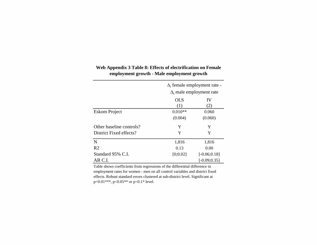
OLS IV(1) (2)

Eskom Project 0.010** 0.060(0.004) (0.060)

Other baseline controls? Y YDistrict Fixed effects? Y Y

N 1,816 1,816R2 0.13 0.00Standard 95% C.I. [0;0.02] [-0.06;0.18]AR C.I. [-0.09;0.35]

t female employment rate - t male employment rate

Table shows coefficients from regressions of the differential difference in employment rates for women - men on all control variables and district fixed effects. Robust standard errors clustered at sub-district level. Significant at p<0.01***, p<0.05** or p<0.1* level.

Web Appendix 3 Table 8: Effects of electrification on Female employment growth - Male employment growth

District has high

electrification rates

District has low

electrificaton rates

Difference Significant?

(1) (2) (3) (4)Fraction of adult who outmigrate 0.39 0.43 -0.04 **Mean yrs of education of adults remaining 6.99 6.54 0.46 ***Mean yrs of education of outmigrant adults 7.21 6.83 0.38 **Mean employment rate among adults remaining 0.38 0.36 0.01Mean employment rate among outmigrants 0.18 0.18 0.00

Web Appendix 3 Table 9: Characteristics of outmigrants and incumbents by district-level electrification status in rural KZN: LFS 2002 data

Table shows descriptive statistics for adult Africans attached to households in rural KZN and enumerated in the September 2002 Labor Force Survey. Means are weighted using survey weights. Outmigrants are individuals identified by the household as belonging to the household, but who are outmigrants. There are 3,201 adults who are not migrants, and 2,146 adults who are outmigants. I define high electrification areas as any magisterial districts in which more than 40% of the households have electric lighting: 66% of individuals live in such areas. The remaining 34% of individuals live in areas where less than 25% of households have electric lighting (there is no density in between 25 and 40% coverage). Significant differences in variable means between high and low electrification areas are presented in columns (3) and (4) (t-tests).

Web Appendix 4: Measurement error

1 Measurement error in the Census data: Employment

The Census data undoubtedly measures employment with some error. While the employment

questions are broad, the Census does not probe for employment information as the household

surveys do. This section discusses the extent of this measurement error by comparing the

Census data to individual level household survey data.

In Web Appendix 4 Table 1, I present population totals and employment rates for six

different surveys: columns (1) and (4) present household-level data from the 1996 October

Household Survey and the 2001 September Labor Force Surveys. These are the closest sur-

veys we have to the relevant Census years and I use the weights in these surveys (constructed

using the relevant Census as a benchmark) to create population totals and employment rates.

In columns (2) and (4), I use the micro data from the 10% sample of the Census in 1996

and 2001 to create the same statistics using the Census weights; and in columns (3) and (6)

I present the statistics taken from the 100% Census community databases in 1996 and 2001.

Note that the unit of observation is the individual in columns (1), (2), (4) and (5) and the

community in columns (3) and (6). Another important difference is that the individual level

data in the Census and household surveys can only be restricted to African adults living in

rural KZN while the Census community data can be disaggregated further to include adult

Africans living in tribal areas of KZN. Tribal areas refer to the former homelands.

The difference between columns (1) and (2), and between (4) and (5) is largely the result

of differences in the Census questions for employment versus the more detailed household

survey questions. The difference between columns (2) and (3), and columns (5) and (6) is

due to a restriction to tribal areas as well as the use of communities (rather than individuals)

as the unit of observation.

The individual Census and household survey data provide population totals that are not

substantially different from each other in most cases (the largest difference is in the male

population total in 2001). However, employment rates are quite different across household

survey and Census data. In every case, employment rates are lower in the 10% Census data

compared with the 1996/2001 household survey data. The gaps also seem to be larger in

2001 than in 1996.

In addition to these differences over time in how closely the individual level data corre-

spond, there are differences between the community data and the individual Census data. In

every year, for men and for women, the Census community data present lower employment

rates: between one quarter and one half of the employment rate is measured in the commu-

nity data. A large part of the explanation for this is that the community data are restricted

1

to tribal areas, which are not identical to all of the rural areas in the province (the Census

community data does not provide a clean variable to separate rural areas into tribal/non-

tribal). Hence individuals who live in rural communities with better average labor market

outcomes than in the tribal, rural areas of the province are excluded from the community

level data.

Web Appendix 4 Table 2 shows correlations between the individual and community Cen-

sus data for different years and for men and women at the magisterial district level. The

first four columns show that the community census employment data predict only a frac-

tion of the individual census employment data and that the fraction explained for women is

higher than it is for men. The final two columns show the correlation between the change

in employment rates measured at the individual level and the change in employment rates

measured at the community level. Again, more of the change in female employment at the

individual level is predicted by the change in female employment in the community data than

for men. This suggests that the Census community data may undercount male employment

to a larger extent than female employment.

There are a few important points to note from Web Appendix 4 Table 1:

• The Census community data that is restricted to tribal areas under-counts employment,

relative to all rural areas.

• The 2001 Census data (both individual and community data) measure lower levels of

employment compared to the household survey data. This is probably due to the way

the Census asked about employment in 2001: “Did you work for at least 1 hour last

week?” compared with the 1996 question, “Did you work for a formal wage/salary,

in informal work, or on a farm last week?” The 2001 question may not have been

interpreted to include informal sector work or farm work by respondents in 2001, so

the main types of employment that are under-counted in 2001 are probably these

types of jobs. As long as the prevalence of these jobs is uncorrelated with gradient,

then under-counting of employment in the 2001 data should not be problematic for the

paper’s main research design.

• Changes in employment in the Census community data more strongly predict changes

in employment in the individual level data for women compared to men. This suggests

that the community level data may be missing more of the employment story for men,

than for women, in these areas.

• Even though the Census community data under-counts employment, the strong mes-

sage from the individual level data is that there are very low levels of employment

2

in these rural areas: under 50% of men are employed and under 30% of women are

employed. These employment rates fall even further when we restrict to tribal areas

of the province in using the Census community data. The low levels of employment in

these areas are not an artifact of mis-measured (i.e. missing) employment.

• Finally, focusing on the occupation distribution for men and women, the individual

Census data count fewer men and women employed in agriculture than the household

surveys do. Agricultural employment in both of the individual sources is higher than in

the Census community data - bearing in mind that the community data count people

living only in tribal areas - and yet is still very low, below 10%. Regardless of which

data set is considered, only a small fraction of individuals work in agriculture in the

rural areas of KZN.

2 Measurement error in the electrification project variable

Since Eskom region boundaries do not line up with Census boundaries, I assign values of Tjdt

in the following way: for any community that lies even partially inside an Eskom project

area, all information from that project is assigned to that community. This means some

communities are assigned full electrification status when only a fraction of households in

the area are electrified. In addition, non-NEP electrification continued during this period in

areas where households were willing to pay for their connections.

Measurement error in the binary project status variable could contribute to the difference

between OLS and IV coefficients. OLS will underestimate the effect of electricity on outcomes

when there is a negative covariance between δj and ∆Tjdt (which I have argued is likely) and

when ∆Tjdt is measured with error. However, the valid IV that is uncorrelated with δj +∆εjt

will tend to be correlated with any non-classical measurement error in the binary variable

∆Tjdt. In this situation, even if the instrument deals with the omitted variables bias, the

measurement error in ∆Tjdt could lead to an upwards-biased IV estimator.1

To get a sense of how much of the difference in OLS and IV results is due to measurement

error, I restrict to samples where I expect ∆Tjdt to be measured with less error. The first

two columns of Web Appendix 4 Table 4 reproduce the main result for females in the full

sample while columns (3) to (6) present results for successive sample limitations. To identify

communities where projects had greater coverage, I exclude electrified areas with less than

a 10 percent change in coverage of electric lighting, and areas where the connection rate

1This result is conditional on the measurement error in electrification status not being too extreme (Kaneet al, 1998). See Bound and Solon (1999) and Kane, Rouse and Staiger (1998) for a discussion of what theIV estimator is consistent for in the presence of non-classical measurement error.

3

between 1996 and 2001 was under 80 percent of households. All communities that did

not have an electricity project during the period are included in all columns. Under the

first restriction in columns (3) and (4), the OLS coefficient rises substantially and the IV

coefficient is the same as the main result at 13 percentage points. The movement in the OLS

coefficient suggests that there is some measurement error is present in the electrification

variable. Columns (5) and (6) impose the second restriction. Again, the OLS estimate is

large and positive and the IV result is now slightly higher than the main result (at 0.155),

although neither is statistically significant due to the smaller sample size.

Although effects estimated under the OLS specification for these sub-samples are between

1 and 1.2 percentage points higher than the OLS result for the full sample, they are still well

smaller than the IV results. This is evidence that measurement error in the electrification

dummy alone is unable to account for the entire gap between OLS and IV estimates.

References

Bound, John and Gary Solon, “Double Trouble: on the value of twins-based estimation

of the returns to schooling,” Economics of Education Review, 1999, 18, 169–182.

Kane, Thomas, Cecilia Elena Rouse, and Douglas Staiger, “Estimating returns to

schooling when schooling is misreported,” 1998. NBER Working Paper No. 7235.

4

OHS 1996 10% Census 100% Census LFS 2001 10% Census 2001 100% Census

Unit and place of observationIndiv. RURAL Indiv. RURAL Comm. TRIBAL Indiv. RURAL Indiv. RURAL Comm.

TRIBALPanel A: WomenPopulation totals 1,398,856 1,299,475 709,285 1,144,854 1,442,057 839,521Total employment/populatio 0.19 0.13 0.07 0.28 0.13 0.07Occupational distribution Managers, profs, assoc. profs 0.03 0.02 0.02 0.03 0.02 0.02Clerks 0.01 0.00 0.00 0.01 0.01 0.00Services 0.02 0.01 0.00 0.03 0.01 0.00Agriculture1 0.01 0.01 0.00 0.01 0.01 0.00Crafters 0.01 0.01 0.00 0.01 0.01 0.00Machine Operators 0.00 0.00 0.00 0.02 0.00 0.00Elementary Occupations2 0.09 0.07 0.03 0.16 0.06 0.04Missing occupations data 0.01 0.02 0.01 0.00 0.02 0.00

Panel B: MenPopulation totals 1,036,785 993,888 504,272 777,350 1,125,483 617,858Total employment/populatio 0.39 0.25 0.14 0.38 0.19 0.10Occupational distribution Managers, profs, assoc. profs 0.04 0.01 0.02 0.03 0.02 0.02Clerks 0.01 0.00 0.01 0.01 0.01 0.01Services 0.06 0.02 0.01 0.04 0.02 0.00Agriculture1 0.01 0.02 0.00 0.03 0.01 0.00Crafters 0.04 0.04 0.02 0.07 0.03 0.01Machine Operators 0.07 0.04 0.02 0.09 0.03 0.02Elementary Occupations2 0.13 0.07 0.03 0.11 0.06 0.04Missing occupations data 0.02 0.05 0.03 0.00 0.02 0.00

1996 2001

Web Appendix 4 Table 1: Comparing measures of employment in the Census and October Household/Labor Force Surveys

Notes: Table shows population totals and means from the October Household Survey (OHS) microdata, the Labor Force Survey (LFS) microdata, the 10% Census microdata and 100% Census community aggregate data. The sample is restricted to rural Africans living in KZN, aged 15-59 inclusive. Means and totals from the OHS/LFS/10% Census data are weighted using population weights provided in each survey. Agriculture 1 includes skilled and subsistence agriculture. Elementary occupations 2 include domestic workers. Census Community data are weighted by the number of people in each community.

Census Individual

2001

Census Individual

1996

Census Individual

2001

Census Individual

1996(1) (2) (3) (4) (5) (6)

Female employment, Community, 2001 0.627***(0.08)

Female employment, Community, 1996 0.508***(0.08)

Male employment, Community, 2001 0.284***(0.05)

Male employment, Community, 1996 0.340***(0.04)

Female employment, Community 0.384***(0.09)

Male employment, Community 0.140***(0.05)

N 42 42 42 42 42 41R2 0.55 0.44 0.39 0.33 0.17 0.01

Female empl.

Individual

Male empl.

Individual

Table shows coefficients (standard errors) from OLS regressions of employment rates measured in the individual Census data on employment rates measured in the aggregate Census data, where data from each Census has been aggregated up to the magisterial district level. Robust standard errors in parentheses. Significance at *** p<0.01, ** p<0.05, * p<0.1. variables refer to change in the employment rate between 1996 and 2001.

Web Appendix 4 Table 2: Correlation between community Census and individual Census employment dataFemale employment Male employment

Females Males

Community - Community - Community - Community - [2001 nderestimate

[2001 nderestimate

Females Males

Web Appendix 4 Table 3: Comparing the difference in employment measurement error gaps by gradient (OLS regressions)

Co u yIndividual data,

2001

Co u yIndividual data,

1996

Co u yIndividual data,

1996

Co u yIndividual data,

2001

underestimate - 1996

underestimate]

underestimate - 1996

underestimate](1) (2) (3) (4) (5) (6)

Gradient aggregated to MD -0.00311** -0.00388** -0.00631*** -0.004 0.001 -0.002gg g(0.001) (0.002) (0.002) (0.003) (0.001) (0.002)

N 41 41 41 41 41 41R2 0.11 0.08 0.08 0.04 0.01 0.01

*** p<0.01, ** p<0.05, * p<0.1, Robust standard errors in parentheses. Each coefficient is from a regression of the outcome variable on land gradient. The first four columns use the (community - individual data) difference in employment rates wthin a year as the outcome variable. The final two columns use the difference in the difference in employement rates across time as the outcome variable. The unit of observation is the magisterial district.

Outcome is ∆t in female employment

OLS IV OLS IV OLS IV(1) (2) (3) (4) (5) (6)

Eskom Project -0.001 0.095* 0.009 0.095 0.011 0.082(0.005) (0.055) (0.007) (0.060) (0.009) (0.087)

N 1,816 1,816 1,461 1,461 1,273 1,273

Web Appendix 4 Table 4: Contribution of measurement error in electrification project status to female employment result

Full sampleRestricted to areas with

> 10% change in electricity coverage

Restricted to areas with over 80% coverage by

2001

Table shows the Eskom project coefficient (s.e.) from an OLS or IV regression of the change in female employment on all controls as described in Table 3, for different samples: the full sample in columns (1) and (2), the sample restricted to areas with a large change in electric lighting in columns (3) and (4), and the sample restricted to areas with the highest levels of electric lighting use by 2001 in the last two columns. Robust standard errors clustered at sub-district level. Significant at p<0.01***, p<0.05** or p<0.1* level.