arX

iv:1

109.

0290

v3 [

hep-

th]

15

Nov

201

1

The effective action of Double Field Theory

Gerardo Aldazabala,b, Walter Baronc, Diego Marquesd

and Carmen Nunezc,e

aCentro Atomico Bariloche, bInstituto Balseiro (CNEA-UNC) and CONICET

8400 S.C. de Bariloche, Argentina.

c Instituto de Astronomıa y Fısica del Espacio (CONICET-UBA)

C.C. 67 - Suc. 28, 1428 Buenos Aires, Argentina.

dInstitut de Physique Theorique, CEA/ Saclay , 91191 Gif-sur-Yvette Cedex, France.

eDepartamento de Fısica, FCEN, Universidad de Buenos Aires

Abstract

We perform a generalized Scherk-Schwarz dimensional reduction of Double Field Theory

on a twisted double torus. The four dimensional effective action is shown to exactly

reproduce the bosonic electric sector of gauged N = 4 supergravity. We present explicit

expressions for the gaugings in terms of the twists, and analyze the associated string

backgrounds. This framework provides a higher dimensional origin of the gaugings in

terms of generalized fluxes.

Contents

1 Introduction 1

2 Review of Double Field Theory 4

3 Scherk-Schwarz dimensional reduction 6

4 The effective action of DFT and gauged N = 4 supergravity 13

4.1 Review of gauged N = 4 supergravity . . . . . . . . . . . . . . . . . . . . . 14

4.2 Comparison with the effective action of DFT . . . . . . . . . . . . . . . . . 16

4.2.1 The O(6, 6) sector . . . . . . . . . . . . . . . . . . . . . . . . . . . . 16

4.2.2 Including vectors . . . . . . . . . . . . . . . . . . . . . . . . . . . . 18

4.2.3 Rescaling symmetry gaugings . . . . . . . . . . . . . . . . . . . . . 20

5 (Non)geometric string backgrounds 22

5.1 Reduction on a twisted double torus . . . . . . . . . . . . . . . . . . . . . 22

5.2 Generalized fluxes and superstring compactifications . . . . . . . . . . . . . 25

5.3 Type I interpretation . . . . . . . . . . . . . . . . . . . . . . . . . . . . . . 30

6 Conclusions 31

A Appendix 32

A.1 Gauging away β-transformations . . . . . . . . . . . . . . . . . . . . . . . 32

A.2 A single flux example . . . . . . . . . . . . . . . . . . . . . . . . . . . . . . 34

1 Introduction

Flux compactifications of string theory [1] lead to gauged supergravities [2], providing an

efficient mechanism of moduli stabilization and spontaneous supersymmetry breaking. An

intriguing puzzle is that gauged supergravity contains more gaugings than those that can

be reached through geometric compactifications of the different string effective actions or

1

string supergravities. The presence of additional (non-geometric) gaugings suggests that

some features of string compactifications have not yet been properly taken into account.

The missing gaugings could be obtained by invoking U-duality arguments at the level

of the dimensionally reduced effective actions [3]-[6]. This approach corresponds to the

dotted (blue) path in Figure 1. Although efficient in generating the full set of gaugings,

this procedure presents the disadvantage of leaving many of them unexplained in terms

of a higher dimensional origin. For instance, enforcing T-duality invariance requires the

introduction of non-geometric fluxes. This can be seen by comparing the effective four

dimensional superpotentials arising in orientifold compactifications of type IIA and IIB

ten dimensional supergravity actions, where a broader class of internal spaces is needed

to have a geometric interpretation.

The concepts of Generalized Complex Geometry [7]-[9], non-geometry [10, 11] and

double geometry [12]-[18] were proposed as suitable frameworks to deal with this situation

(see also [19, 20] for extensions to M-theory). By treating the symmetries of the NSNS

antisymmetric tensor field and diffeomorphisms on an equal footing, some of the properties

of T-duality are naturally incorporated. Inspired by this approach, a way to obtain the

usual contribution of the locally geometric Q-flux [21] to the four-dimensional effective

action, from a ten dimensional one, was recently proposed in [22].

On the other hand, there have also been attempts to promote U-duality to a symmetry

at the level of the higher dimensional supergravity. For T-duality this was successfully

achieved by Double Field Theory (DFT), originally formulated in [23]-[26] and extended in

[27]-[37]. This attempt is represented in the figure with the dashed (red) arrow. The idea,

which we review in Section 2, was to introduce additional coordinates to the standard

space-time embedding of closed strings in toroidal backgrounds, dual to winding. In DFT

the fields depend on both sets of coordinates and this gives rise to a 2D-dimensional

theory formulated on a double space. The stringy nature of the theory is manifested in

the fact that DFT is T-duality invariant, so it promotes a string duality to a symmetry.

In this work we follow the path indicated by the two solid (green) arrows in Figure 1.

First, by performing a generalized Scherk-Schwarz dimensional reduction [38] on a twisted

double torus we obtain the effective action of DFT. This procedure allows to identify the

2

NS-NS D-dim

sugra

2D-dim DFT

Bosonic n-dim

gauged sugra

(geometric fluxes)

Bosonic n-dim

gauged sugra

(dual fluxes)

Bosonic electric

gauged N = 4

sugra

O(D,D)

O(d, d)

Twisted T d Twisted T d,d

n=4d=6

Figure 1: From string supergravity to four dimensional N = 4 gauged supergravity.

new degrees of freedom present in DFT as the origin of the missing (non-geometric)

gaugings. The computation, for an arbitrary number of dimensions, is performed in

Section 3. The reduced theory is a generalization of that found in [39]. Interestingly

enough, it includes geometric fluxes as well as the locally (but not globally) geometric

fluxes Q and the locally non-geometric fluxes R. Besides, it inherits a remnant gauge

symmetry from DFT based on the C-bracket, and a (would be) global O(d, d) invariance

which is broken by the fluxes.

In Section 4 we show that the four dimensional effective action with six internal dimen-

sions is dual to the bosonic electric sector of gauged N = 4 supergravity, as formulated

in [40]. This corresponds to the second solid (green) arrow. In order to recover the full

set of gaugings, we show how to generalize the Scherk-Schwarz reduction to include the

fundamental fluxes ξ+M . Additionally, we enhance the O(D,D) symmetry of DFT to

O(D,D +N) by adding N generalized vector fields along the lines of [41] and [28].

Section 5 is devoted to the analysis of the string (non)geometric backgrounds and the

fluxes they give rise to. We show that the internal space can be thought of as a twisted

double torus. Alternative interpretations of our results from the point of view of super-

string compactifications are discussed. In particular we show that the resulting effective

theory can be seen either as a bosonic sector of heterotic string compactification, extended

3

by T-duality [3, 6], or as a bosonic sector of a Type IIB orientifold compactification [5, 42].

Finally, the conclusions in Section 6 contain a summary of our results. We include

an Appendix illustrating how single-flux string backgrounds are encoded in the twisted

double torus.

2 Review of Double Field Theory

D-dimensional closed strings on toroidal backgrounds carry both momentum and winding,

the former being dual to space-time coordinates. Double Field Theory was constructed

out of the idea of assigning dual coordinates also to winding. While in string supergrav-

ities in D dimensions fields depend only on space-time coordinates, DFT incorporates a

dependence also on the coordinates dual to winding. For this reason, it is a theory defined

in a doubled space with coordinates XM = (X µ, Xµ). The most remarkable feature of

this theory is that it is invariant under T-dualities, and more generally under the full

O(D,D) group associated to the isometries of the doubled torus. In this way, DFT is a

field theory that takes “stringy” features into account by promoting a string duality to a

symmetry.

In this section we present a brief review of the generalized metric formulation of

DFT, mainly to exhibit the results that we will use throughout the paper. The notation

basically coincides with the standard conventions, but we put a hat on all fields and

indices to facilitate the reading of the forthcoming sections.

The building block of the theory is the generalized 2D × 2D metric

HMN =

gµν −gµρBρν

Bµρgρν gµν − Bµρg

ρσBσν

, (2.1)

constructed out of the D-dimensional metric gµν(Xµ, Xµ) and the D-dimensional 2-form

field Bµν(Xµ, Xµ). This generalized metric is an element of O(D,D), so it preserves the

metric of the group that we take of the following form

I =

0 1D

1D 0

. (2.2)

4

In addition, the model also contains an O(D,D) invariant dilaton

e−2d =√

|g|e−2φ . (2.3)

The background independent formulation of DFT is defined by an action that can be

written in a compact form (up to total derivatives) in terms of a generalized Ricci scalar

as

SDFT =

∫

dDXdDX e−2d R(H, d) , (2.4)

where R is defined by

R(H, d) = 4HMN∂M∂N d− ∂M∂NHMN − 4HMN∂M d∂N d+ 4∂MHMN∂N d

+1

8HMN∂MHKL∂NHKL −

1

2HMN∂MHKL∂KHNL . (2.5)

When the coordinates dual to winding are frozen, i.e. ∂X • = 0, this action reduces to the

standard NS-NS bosonic sector of the D-dimensional string supergravities. The theory is

constrained by a world-sheet level-matching condition that can be written as

∂M∂M • = 0 , (2.6)

and the construction of the action (2.4) requires the so called “strong constraint” stating

that all fields and their products (represented by • above) must be annihilated by the

differential operator (2.6). The strong constraint implies that locally there is always an

O(D,D) transformation that rotates into a frame in which fields depend only on half of

the coordinates.

Regarding symmetries, the action is manifestly invariant under global O(D,D) trans-

formations acting as

HMN → U AMHABU

BN , d→ d , U ∈ O(D,D) . (2.7)

In addition it has the following gauge symmetry

δξd = ξM∂M d−1

2∂M ξ

M ,

δξHMN = ξP∂P HMN +(

∂M ξP − ∂P ξM)

HP N +(

∂N ξP − ∂P ξN)

HMP . (2.8)

5

This transformation rule is an O(D,D) covariant extension of the standard Lie derivative

that governs infinitesimal diffeomorphisms. Generalized Lie derivatives acting on vectors

can be constructed as

LξAM = ξN∂NAM + (∂M ξN − ∂N ξM)AN , (2.9)

such that the transformation rules (2.8) read δξHMN = LξHMN . The gauge transforma-

tions then close under the so-called C-bracket, defined as

[

Lξ1, Lξ2

]

AM = −L[ξ1,ξ2]CAM , (2.10)

where[

ξ1, ξ2

]M

C= 2ξN[1 ∂N ξ

M2] − ξP[1∂M ξ2]P . (2.11)

For further insight on DFT we refer to the original works [23]-[26] and to their many

extensions [27]-[37].

3 Scherk-Schwarz dimensional reduction

In this section we perform the twisted dimensional reduction of DFT and compute the

effective action. The starting point for the compactification procedure is the generalized

2D-dimensional double space on which DFT is defined. We identify n of its coordinates

with space-time coordinates and other n with their duals. The first step is to compactify

this double space-time on a double torus of vanishing dual radius, so that the usual

space-time is naturally decompactified. We are therefore effectively left with a (n +

2d)−dimensional space (D = n+ d) that we compactify on a twisted T d,d torus to obtain

the n-dimensional effective theory of DFT.

Throughout the paper we use many different indices. The original formulation of

DFT in 2D-dimensions is based on the usual D “string” coordinates and the remaining

D correspond to the dual space. After dimensionally reducing in a 2d-dimensional space,

the effective action is an n = D − d dimensional theory (provided the coordinates dual

to space-time are taken to vanish). Of course, at the end of the day our main interest is

in D = 10, d = 6 and n = 3 + 1, but since most computations can be performed without

6

explicitly specifying the dimensions, we keep the results as general as possible. We use

the following notation:

Curved and tangent indices are respectively

M, N , O, P , · · · ∈ 0, 1, 2, . . . , 2D − 1 , A, B, C, D, · · · ∈ 0, 1, 2, . . . , 2D − 1 , (3.1)

for the full 2D space;

µ, ν, ξ, ρ, σ, · · · ∈ 0, 1, 2, . . . , D − 1 , m, n, o, p, q, · · · ∈ 0, 1, 2, . . . , D − 1, (3.2)

for the D-dimensional “stringy” coordinates;

M,N,O, P, · · · ∈ 1, 2, . . . , 2d , A, B, C,D, · · · ∈ 1, 2, . . . , 2d, (3.3)

for 2d-dimensional internal and dual coordinates (which we denote by YM);

µ, ν, ρ, σ, · · · ∈ 0, 1, . . . , n− 1 , m, n, p, q, · · · ∈ 0, 1, . . . , n− 1, (3.4)

for spacetime and

α, β, γ, δ, · · · ∈ 1, 2, . . . , d , a, b, c, d, · · · ∈ 1, 2, . . . , d, (3.5)

for the d-dimensional internal indices (with the corresponding coordinates denoted as yα).

Dual coordinates are yα and we usually write YA = (ya, y

a).

As we have seen, the degrees of freedom in DFT are represented by an invariant dilaton

d defined in (2.3) and a generalized 2D × 2D metric (2.1), namely

HMN =

Hµν Hµν

Hµν Hµν

=

gµν −gµρBρν

Bµρgρν gµν − Bµρg

ρσBσν

. (3.6)

This metric can be constructed out of a vielbein with triangular1 form, i.e.

E =

(e−1)T −(e−1)T B

0 e

, (3.7)

which is related to (3.6) through

H = ET η E , η =

η−1 0

0 η

, (3.8)

1We refer to the Appendix for a discussion on the generality of considering the triangular gauge.

7

where η = diag(−+ · · ·+).

We have defined the D-dimensional fields that parameterize the generalized metric,

namely the Kalb-Ramond field B and the D-bein e associated to the metric

gµν = emµηmnenν =

(

eT ηe)

µν. (3.9)

These can then be written as usual in terms of the compactified degrees of freedom as

gµν =

gµν + hγδAγµAδ

ν Aγµhγβ

hαγAγν hαβ

, Bµν =

Bµν −BβµBαν bαβ

. (3.10)

From the n-dimensional point of view, the D-dimensional metric decomposes into an

n-dimensional metric gµν , d vectors Aαµ and d(d+ 1)/2 real scalars hαβ . The B-field also

decomposes into an n-dimensional 2-form Bµν , d vectors Bαµ (which we will further relate

to Bµν and Bαν in equation (3.18)) and d(d− 1)/2 real scalars bαβ .

Having set the structure of the (compactified) fields, we proceed with the Scherk-

Schwarz twist. The global symmetry of the action that we intend to twist is the O(D,D)

invariance defined in (2.7). We perform a U ∈ O(D,D) transformation of the fields,

and propose as an ansatz that the fields only depend on space-time coordinates x while

the dependence on the internal coordinates Y enters through the group element of the

transformation, U(Y). Since d is O(D,D) invariant, it is natural to propose for it a trivial

ansatz d(x,Y) = d(x). Instead, inspired by (2.7), for the generalized metric we propose

the following decomposition:

HMN(x,Y) = U AM(Y) HAB(x) U

BN(Y) , (3.11)

which in terms of the vielbein reads

E AM(x,Y) = E AB(x) UBM(Y) . (3.12)

In triangular gauge (3.7), equation (3.12) can be rewritten as

(e−1)µm(x,Y) −(e−1)ρm(x,Y)Bρν(x,Y)

0 enν(x,Y)

=

(e−1)pm(x) −(e−1)rm(x)Brq(x)

0 enq(x)

×U (Y) .

(3.13)

8

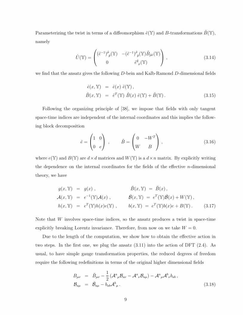
Parameterizing the twist in terms of a diffeomorphism e(Y) and B-transformations B(Y),

namely

U(Y) =

(e−1)µp(Y) −(e−1)ρp(Y)Bρν(Y)

0 eqν(Y)

, (3.14)

we find that the ansatz gives the following D-bein and Kalb-Ramond D-dimensional fields

e(x,Y) = e(x) e(Y) ,

B(x,Y) = eT (Y) B(x) e(Y) + B(Y) . (3.15)

Following the organizing principle of [38], we impose that fields with only tangent

space-time indices are independent of the internal coordinates and this implies the follow-

ing block decomposition

e =

1 0

0 e

, B =

0 −W T

W B

, (3.16)

where e(Y) and B(Y) are d×d matrices andW (Y) is a d×n matrix. By explicitly writing

the dependence on the internal coordinates for the fields of the effective n-dimensional

theory, we have

g(x,Y) = g(x) , B(x,Y) = B(x) ,

A(x,Y) = e−1(Y)A(x) , B(x,Y) = eT (Y)B(x) +W (Y) ,

h(x,Y) = eT (Y)h(x)e(Y) , b(x,Y) = eT (Y)b(x)e +B(Y) . (3.17)

Note that W involves space-time indices, so the ansatz produces a twist in space-time

explicitly breaking Lorentz invariance. Therefore, from now on we take W = 0.

Due to the length of the computation, we show how to obtain the effective action in

two steps. In the first one, we plug the ansatz (3.11) into the action of DFT (2.4). As

usual, to have simple gauge transformation properties, the reduced degrees of freedom

require the following redefinitions in terms of the original higher dimensional fields

Bµν = Bµν −1

2(Aa

µBaν −AaνBaµ)−Aa

µAbνbab ,

Baµ = Baµ − babAbµ . (3.18)

9

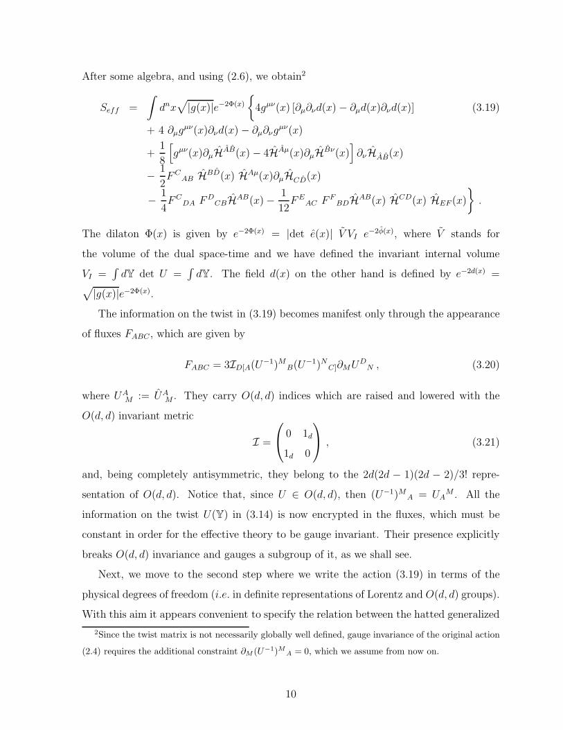
After some algebra, and using (2.6), we obtain2

Seff =

∫

dnx√

|g(x)|e−2Φ(x)

4gµν(x) [∂µ∂νd(x)− ∂µd(x)∂νd(x)] (3.19)

+ 4 ∂µgµν(x)∂νd(x)− ∂µ∂νgµν(x)

+1

8

[

gµν(x)∂µHAB(x)− 4HAµ(x)∂µHBν(x)]

∂νHAB(x)

− 1

2FC

AB HBD(x) HAµ(x)∂µHCD(x)

− 1

4FC

DA FDCBHAB(x)− 1

12FE

AC F FBDHAB(x) HCD(x) HEF (x)

.

The dilaton Φ(x) is given by e−2Φ(x) = |det e(x)| V VI e−2φ(x), where V stands for

the volume of the dual space-time and we have defined the invariant internal volume

VI =∫

dY det U =∫

dY. The field d(x) on the other hand is defined by e−2d(x) =√

|g(x)|e−2Φ(x).

The information on the twist in (3.19) becomes manifest only through the appearance

of fluxes FABC , which are given by

FABC = 3ID[A(U−1)MB(U

−1)NC]∂MUDN , (3.20)

where UAM := UA

M . They carry O(d, d) indices which are raised and lowered with the

O(d, d) invariant metric

I =

0 1d

1d 0

, (3.21)

and, being completely antisymmetric, they belong to the 2d(2d − 1)(2d − 2)/3! repre-

sentation of O(d, d). Notice that, since U ∈ O(d, d), then (U−1)MA = UAM . All the

information on the twist U(Y) in (3.14) is now encrypted in the fluxes, which must be

constant in order for the effective theory to be gauge invariant. Their presence explicitly

breaks O(d, d) invariance and gauges a subgroup of it, as we shall see.

Next, we move to the second step where we write the action (3.19) in terms of the

physical degrees of freedom (i.e. in definite representations of Lorentz and O(d, d) groups).

With this aim it appears convenient to specify the relation between the hatted generalized

2Since the twist matrix is not necessarily globally well defined, gauge invariance of the original action

(2.4) requires the additional constraint ∂M (U−1)MA = 0, which we assume from now on.

10

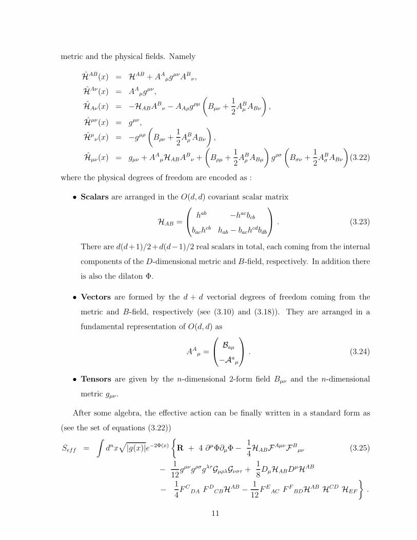
metric and the physical fields. Namely

HAB(x) = HAB + AAµg

µνABν ,

HAν(x) = AAµg

µν ,

HAν(x) = −HABABν − AAρg

ρµ

(

Bµν +1

2AB

µABν

)

,

Hµν(x) = gµν ,

Hµν(x) = −gµρ

(

Bρν +1

2AB

ρ ABν

)

,

Hµν(x) = gµν + AAµHABA

Bν +

(

Bρµ +1

2AB

ρ ABµ

)

gρσ(

Bσν +1

2AB

σABν

)

(3.22)

where the physical degrees of freedom are encoded as :

• Scalars are arranged in the O(d, d) covariant scalar matrix

HAB =

hab −hacbcbbach

cb hab − bachcdbdb

. (3.23)

There are d(d+1)/2+d(d−1)/2 real scalars in total, each coming from the internal

components of the D-dimensional metric and B-field, respectively. In addition there

is also the dilaton Φ.

• Vectors are formed by the d + d vectorial degrees of freedom coming from the

metric and B-field, respectively (see (3.10) and (3.18)). They are arranged in a

fundamental representation of O(d, d) as

AAµ =

Baµ−Aa

µ

. (3.24)

• Tensors are given by the n-dimensional 2-form field Bµν and the n-dimensional

metric gµν .

After some algebra, the effective action can be finally written in a standard form as

(see the set of equations (3.22))

Seff =

∫

dnx√

|g(x)|e−2Φ(x)

R + 4 ∂µΦ∂µΦ−1

4HABFAµνFB

µν (3.25)

− 1

12gµνgρσgλτGµρλGνστ +

1

8DµHABD

µHAB

− 1

4FC

DA FDCBHAB − 1

12FE

AC F FBDHAB HCD HEF

.

11

Here R is the n-dimensional Ricci scalar, and we have defined the field strengths as

FAµν = ∂µA

Aν − ∂νAA

µ − FABCA

Bµ A

Cν ,

Gµρλ = 3∂[µBρλ] − FABCAAµA

BρA

Cλ + 3∂[µA

AρAλ]A, (3.26)

and a covariant derivative for scalars as

DµHAB = ∂µHAB − FCADA

DµHCB − FC

BDADµHAC . (3.27)

The effective theory (3.25) has remnant symmetries that are inherited from the global

symmetry (2.7) and the gauge invariance (2.8) of its parent DFT. Concerning the former,

although the effective theory is written in a manifestly covariant O(d, d) form, the fluxes

explicitly break O(d, d) invariance, which is only recovered if they are treated as spurionic

fields. With respect to gauge invariance, given a 2D-dimensional gauge parameter ξM ,

the gauge transformations (2.8) can be twisted as

ξM(x,Y) =(

U−1(Y))M

A ξA(x) , (3.28)

and, when evaluated on the C-bracket (2.11), the following effective algebra is induced

[δξ1 , δξ2 ]C = δξ3 , ξA3 = −FABC ξB2 ξ

C1 , (3.29)

where the structure constants are given by the fluxes (3.20). In terms of the gauge

parameter ξA(x) the fields transform as

δξgµν(x) = 0 ,

δξd(x) = 0 ,

δξBµν(x) = −12

(

AAµ∂νξA −AA

ν∂µξA)

,

δξAAµ(x) = −∂µξA(x)− FA

BC ξB(x)ACµ ,

δξHAB(x) = −FACD ξC(x)HDB(x)− FBC

D ξC(x)HAD(x) . (3.30)

The twists define the infinitesimal generators of this symmetry group, namely

EA = (U−1) PA EP , (3.31)

which satisfy the following C-algebra

[EA, EB]C = FDAB ED . (3.32)

12

The Jacobiator associated to the C-bracket does not automatically vanish, so it is not a

priori evident whether the fluxes satisfy Jacobi identities or not. To answer this ques-

tion we note that the C-bracket differs from the D-bracket (which, although non skew-

symmetric, does satisfy Jacobi) by a total derivative [26]

[A, B]RD = [A, B]RC +1

2∂R(ANBN) . (3.33)

When particularly evaluated on the twists U(Y), the last term vanishes

∂R(

(U−1)MAIMN (U−1)NB

)

= ∂RIAB = 0 , (3.34)

restoring anti-symmetry and leading to a vanishing Jacobiator. We thus conclude that

the fluxes must be constrained by the usual Jacobi identities

FC[ABF

ED]C = 0 . (3.35)

4 The effective action of DFT and gauged N = 4 su-

pergravity

Setting n = 4 and d = 6, the effective action of DFT derived in the previous section

reduces to a four dimensional gauge theory with an O(6, 6) global invariance. Interestingly

enough, O(6, 6) is the symmetry group of four dimensional gauged N = 4 supergravity.

Therefore, even if the starting DFT does not include supersymmetry, we could expect a

connection with the bosonic sector of gauged supergravity. Indeed, in this Section we show

that the effective action of DFT reproduces the electric bosonic sector of four dimensional

gauged N = 4 supergravity.

We begin by reviewing this theory in the formulation of Schon and Weidner [40] and

then establish the precise correspondence. The notation used in [40] differs from ours,

and the relation between both conventions is specified in Table 1 and in equation (4.13)

below.

13

4.1 Review of gauged N = 4 supergravity

The 4-dimensional ungauged N = 4 supergravity has a global symmetry G = SL(2) ×O(6, 6 +N), whose maximal compact subgroup K = U(1)×O(6)×O(6 +N) is realized

on-shell as a gauge symmetry of the theory. The part of its field content that will be

relevant for our discussion is arranged in a gravity multiplet and 6 +N vector multiplets

involving the following fields:

• The gravity multiplet contains the metric gµν , six vectors Bmµ (m = 1, ..., 6) and

one complex scalar τ parameterizing the coset SU(2)/U(1). It is useful to define

the K invariant matrix

Mαβ =1

Imτ

|τ |2 Reτ

Reτ 1

with SL(2) indices α, β = ±. In addition, it contains four gravitinos ψiµ and four

spin-1/2 fermions ψi (i = 1, ..., 4). The fermions are singlets under G and rotate

among each other through SU(4) ≈ O(6) ∈ K.

• Each vector multiplet contains one vector Aaµ (a labels the vector multiplet), six

real scalars and four spin-1/2 gauginos λia. Again, the index i = 1, ..., 4 is a gauge

index rotated by O(6) ∈ K, and the vector multiplets are rotated among each other

by O(6 +N) ∈ K. All the 6× (6 +N) real scalars parameterize the coset

V AM ∈ O(6, 6 +N)

O(6)× O(6 +N), (4.1)

with M an O(6, 6 +N) index and A splits into (m, a) with m an O(6) index and a

an O(6 +N) index. This vielbein is an element of O(6, 6 +N) so it satisfies

ηMN = −V mM V m

N + V aM V a

N , ηMN = diag(−−−−−−,+...+) . (4.2)

As for τ , one can construct a K-invariant scalar matrix

MMN = VaMVa

N + VmMVm

M . (4.3)

Finally, the 6 vectors of the gravity multiplet together with the 6+N vectors of the vector

multiplets combine to form the electric vector field in the fundamental of O(6, 6 +N)

A M+µ =

Bmµ

Aaµ

. (4.4)

14

In the description of [40], the ungauged theory contains the metric gµν , electric vector

fields A M+µ and scalars τ and MMN as free fields in the Lagrangian, while the dual

magnetic vectors A M−µ and two-form gauge fields BMN

µν and Bαβµν are only introduced

on-shell. The gauging of the global group is parameterized by the embedding tensors in

the following representations of G

fαMNP ∈ (2, 220) , ξαM ∈ (2, 12) . (4.5)

When these gaugings are turned on, some of the fields that were absent off-shell in the

ungauged theory are now present.

The bosonic Lagrangian is a sum of three terms Lbos = Lkin + Lpot + Ltop given by

e−1Lkin =1

2R+

1

16DµMMND

µMMN +1

8DµMαβD

µMαβ

−14Im(τ)MMNHM+

µν HµνN+ +1

8Re(τ) ηMN ǫµνρλHM+

µν HN+ρλ ,

e−1Lpot = −g2

16

f+MNPf+QRSM++

[

1

3MMQMNRMPS +

(

2

3ηMQ −MMQ

)

ηNRηPS

]

+ 3ξM+ ξN+M

++MMN

+ . . . ,

e−1Ltop = −g2ǫµνρλ

ξ+MηNPAM−

µ AN+ν AP+

λ − g

4f+MNRf

R+PQ AM+

µ AN+ν AP+

ρ AQ−

λ

−14ξ+MB

++µν

(

2∂ρAM−

λ − gf M+QR AQ+

ρ AR−

λ

)

+ ... , (4.6)

where the dots involve terms containing magnetic gaugings f−MNP and ξ−M . The covari-

ant derivatives are defined by

DµMαβ = ∂µMαβ + gAMγµ ξ(αMMβ)γ − gAMδ

µ ξ+Mǫδ(αMβ)− + ... ,

DµMMN = ∂µMMN + 2gAP+µ Θ Q

+P (M MN)Q + ... , (4.7)

the field strength by

HM+µν = 2∂[µA

M+ν] − gf M

+NP ANα[µ AP+

ν] +g

2ξM+ B

++µν + ... , (4.8)

and also the following combinations of gaugings were defined

Θ+MNP = f+MNP − ξ+[NηP ]M , f+MNP = f+MNP − ξ+[MηP ]N −3

2ξ+NηMP . (4.9)

15

Finally, we mention that the gaugings must satisfy the following consistency quadratic

constraints

ξM+ ξ+M = 0 , (4.10)

ξP+f+PMN = 0 , (4.11)

3f+R[MNfR

+PQ] + 2ξ+[Mf+NPQ] = 0 , ... (4.12)

4.2 Comparison with the effective action of DFT

Having reviewed the on-shell formulation of N = 4 gauged supergravity, let us proceed

to compare it with (3.25) in the particular case n = 4, d = 6. First we note that since the

effective action of DFT has no SL(2) symmetry mixing electric with magnetic sectors,

we can only hope to reproduce one of these sectors, which we take to be the electric one.

Since the vectors in the effective action of DFT arise only from the metric and B-field,

we must set N = 0. We then show how to relax this restriction and finally, by gauging

the rescaling symmetry, we propose a way to obtain the gaugings ξ+M .

Note that the O(6, 6) metrics employed in (3.21) and (4.2) differ, the relation between

them being

RTηR = I , R =1√2

1 −11 1

∈ SO(12) . (4.13)

Therefore, all the comparisons made in this section are only valid up to a rotation by this

matrix. We implicitly assume this fact.

4.2.1 The O(6, 6) sector

The fluxes in (3.20) belong to the 220 of O(6, 6). It is then natural to identify them with

the electric gaugings and we must then turn off all the magnetic fluxes f−MNP and ξ−M .

There is no other source of deformations so far, so we must also set ξ+M = 0 (the inclusion

of the full set of electric gaugings is discussed in the forthcoming subsections).

To perform the comparison, the effective action of DFT (3.25) must first be taken to

the Einstein frame. The transformation gµν → e2Φgµν gives

16

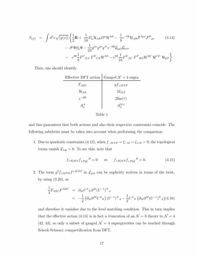
Seff =

∫

d4x√

|g(x)|

1

2R+

1

16DµHABD

µHAB − 1

8e−2ΦHABFAµνFB

µν (4.14)

− ∂µΦ∂µΦ−1

24gµνgρσgλτe−4ΦGµρλGνστ

− e2Φ1

8FC

DA FDCBHAB − e2Φ 1

24FE

AC F FBDHAB HCD HEF

.

Then, one should identify

Effective DFT action Gauged N = 4 sugra

FABC gf+MNP

HAB MMN

e−2Φ 2Im(τ)

AAµ AM+

µ

Table 1

and this guarantees that both actions and also their respective constraints coincide. The

following subtleties must be taken into account when performing the comparison:

1. Due to quadratic constraints (4.12), when f−MNP = ξ−M = ξ+M = 0, the topological

terms vanish Ltop = 0. To see this, note that

f+R[MNfR

+PQ] = 0 ⇔ f+R[MNfR

+P ]Q = 0 . (4.15)

2. The term g2f+MNPf+MNP in Lpot can be explicitly written in terms of the twist,

by using (3.20), as

1

3FABCF

ABC = ∂MUAN∂

M (U−1)NA

= −12

(

∂M∂MUA

N

)

(U−1)NA −1

2UA

N

(

∂M∂M (U−1)NA

)

(4.16)

and therefore it vanishes due to the level matching condition. This in turn implies

that the effective action (4.14) is in fact a truncation of an N = 8 theory to N = 4

[42, 43], so only a subset of gauged N = 4 supergravities can be reached through

Scherk-Schwarz compactification from DFT.

17

3. To make the equivalence evident, the two-form Bµν must be dualized in the effective

action of DFT to give an equivalent theory in terms of a scalar field λ ≡ 2Re(τ).

Introducing λ as a Lagrange multiplier to enforce ǫσµνρ∂σ∂µBνρ = 0, one defines the

following action for Bµν

SB = −∫

d4x

24

√g[

e−4ΦGµνρGµνρ + 2λǫσµνρ∂σ(Gµνρ + FABCAAµA

Bν A

Cρ − 3∂µA

Aν AAρ)

]

.

Here Gµνρ must be eliminated through its equation of motion

Gµνρ = e4Φǫσµνρ∂σλ , (4.17)

which replaced in SB gives

SB = −∫

d4x

24

√ge4Φ

[

6∂σλ∂σλ− 2λǫσµνρ∂σ

(

−FABCAAµA

Bν A

Cρ + 3∂[µA

Aν Aρ]A

)]

.

The first term contributes to the kinetic term for the gravity scalars, and the second

one coincides with the last term in Lkin upon use of quadratic constraints.

4.2.2 Including vectors

We showed above that the effective action of DFT matches the bosonic electric sector of

gauged N = 4 supergravity when the number of vector multiplets is six, i.e. N = 0, and

ξ+M = 0. Here we show how to relax the first restriction.

To increase the number of electric vector fields, we are inspired by the extension of DFT

to the abelian heterotic string performed in [28], where the 2D coordinates X µ, Xµ, µ =

0, . . . , D − 1 are extended by N extra coordinates zi, i = 1, . . . , N and, correspondingly,

the generalized metric HMN is enlarged to a (2D+N)× (2D+N) matrix that naturally

incorporates N additional vector fields V iµ.

We will use the following O(D,D +N) metric

IMN =

I µν I µν I µiIµν Iµν IµiIiν Iiν Iij

=

0 1D 0

1D 0 0

0 0 1N

. (4.18)

We formally keep the action and the form of the gauge transformations but with

respect to the enlarged generalized metric HMN introduced in [28], namely

18

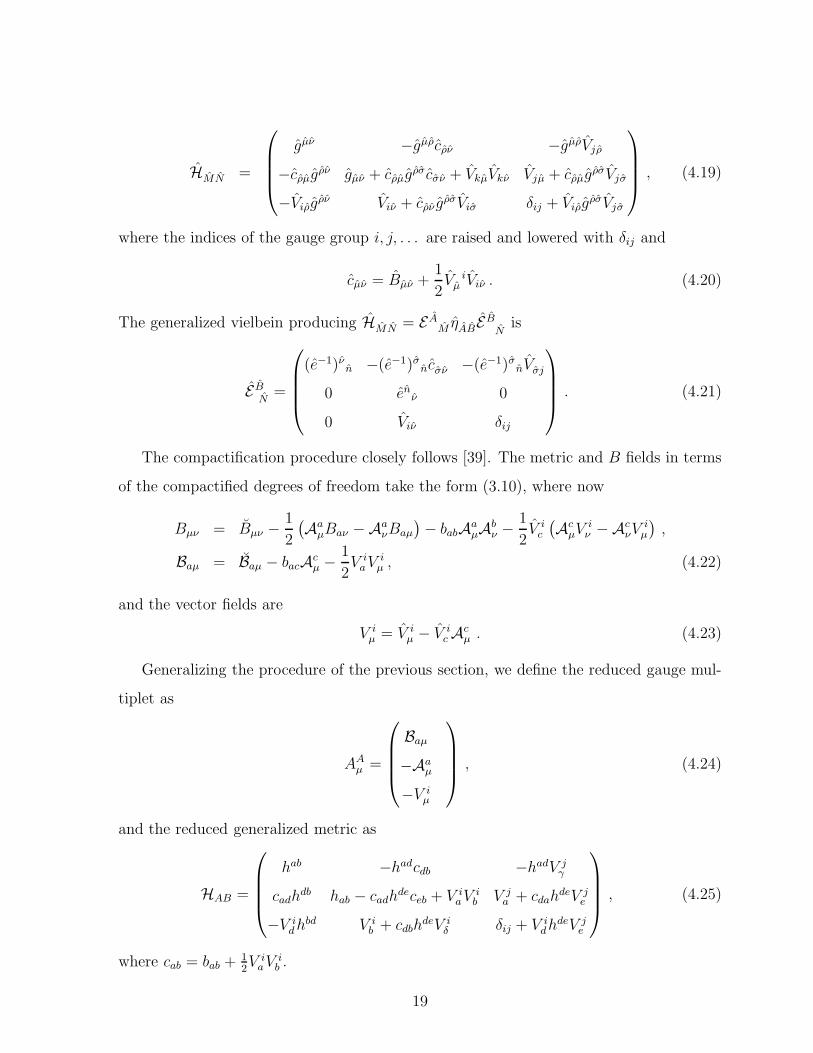
HMN =

gµν −gµρcρν −gµρVjρ−cρµgρν gµν + cρµg

ρσ cσν + VkµVkν Vjµ + cρµgρσVjσ

−Viρgρν Viν + cρν gρσViσ δij + Viρg

ρσVjσ

, (4.19)

where the indices of the gauge group i, j, . . . are raised and lowered with δij and

cµν = Bµν +1

2V iµ Viν . (4.20)

The generalized vielbein producing HMN = E AM ηABE BNis

E BN=

(e−1)ν n −(e−1)σ ncσν −(e−1)σ nVσj

0 enν 0

0 Viν δij

. (4.21)

The compactification procedure closely follows [39]. The metric and B fields in terms

of the compactified degrees of freedom take the form (3.10), where now

Bµν = Bµν −1

2

(

AaµBaν −Aa

νBaµ

)

− babAaµAb

ν −1

2V ic

(

AcµV

iν −Ac

νViµ

)

,

Baµ = Baµ − bacAcµ −

1

2V iaV

iµ , (4.22)

and the vector fields are

V iµ = V i

µ − V icAc

µ . (4.23)

Generalizing the procedure of the previous section, we define the reduced gauge mul-

tiplet as

AAµ =

Baµ−Aa

µ

−V iµ

, (4.24)

and the reduced generalized metric as

HAB =

hab −hadcdb −hadV jγ

cadhdb hab − cadhdeceb + V i

aVib V j

a + cdahdeV j

e

−V idh

bd V ib + cdbh

deV iδ δij + V i

dhdeV j

e

, (4.25)

where cab = bab +12V iaV

ib .

19

The global symmetry to be twisted is now O(D,D + N) and we extend the ansatz

(3.11) for the generalized metric as

HMN (x,Z) = U AM(Z) HAB(x) U

BN (Z) , (4.26)

where Z = (Y, z) and U ∈ O(D,D +N). In terms of the vielbein, it reads

E AM(x,Z) = E AB(x) U

BM(Z) , (4.27)

which can be rewritten in matricial form as

(e−1)T (x,Z) −(e−1)T (x,Z)c(x,Z) −(e−1)T (x,Z)V T (x,Z)

0 e(x,Z) 0

0 V (x,Z) 1

=

(e−1)T (x) −(e−1)T (x)c(x) −(e−1)T (x)V T (x)

0 e(x) 0

0 V (x) 1

× U(Z) . (4.28)

Parameterizing the twist in terms of diffeomorphisms e, B and V transformations, namely

U(Z) =

(e−1)T − (e−1)T c − (e−1)T V T

0 e 0

0 V 1

, (4.29)

the ansatz gives the following D-dimensional gauge fields

V (x,Z) = V (Z) + e(Z)V (x) . (4.30)

Now everything goes on exactly as before. The reduced effective action has the same

form of the previous section, namely (3.25), with the obvious extension in the values taken

by the indices and the inclusion of N extra vector fields V iµ in the definition (4.24).

4.2.3 Rescaling symmetry gaugings

In this section we propose a way to obtain the gaugings ξ+M in the (2, 12) representations

of SL(2)×O(6, 6). For simplicity here we restrict to the N = 0 case, but the results can

be extended if heterotic vector multiplets are introduced as in the previous subsection

20

and their rescaling taken into account. To facilitate the presentation, in this subsection

we turn off the gaugings in the (2, 220).

In [44], a rescaling symmetry of the NS-NS sector of the heterotic theory was twisted,

and it was shown that this gives rise to the gaugings ξ+m withm = 1, . . . 6. This symmetry

acts by rescaling the metric and B-field, and by shifting the dilaton, and it is explicitly

broken in DFT due to the dependence on the dual coordinates. However, at a formal level

DFT is invariant under a global symmetry given by

d→ d± γ , HMN → OMP HP QON

Q , O =

eγ 0

0 e−γ

, (4.31)

whenever the following relation holds

OPM∂P → e±γ∂M , (4.32)

i.e., when either

∂m • = 0 (−) (4.33)

or

∂m • = 0 (+) . (4.34)

While the former (4.33) corresponds to the case analyzed in [44], the later is only possible

due to the doubling of the coordinates, and symmetry arguments suggest that they should

give rise to the ξm+ gaugings. Here we use the covariant notation (4.31), but one should

keep in mind that the extension of the symmetry is only possible if covariance is broken

through either (4.33) or (4.34).

The compactification procedure is equivalent to the one before. One transforms the

fields and makes the transformations carry the internal dependence

d(x,Y) = d(x)± γ(Y) , HMN (x,Y)→ OMP (Y)HP Q(x)ON

Q(Y) . (4.35)

The ± depends on whether (4.33) or (4.34) is chosen.

The comparison of the effective action with gauged N = 4 supergravity is not straight-

forward, and one must use the dualizations of [44]. Instead of dualizing the B-field into

the axion of [40], one must integrate the AM−µ fields out and use the local gauge invari-

ance under (axionic) rescaling shifts to gauge away the axion Imτ = 0. This yields the

21

following equivalent formulation of gauged N = 4 supergravity when only ξ+ gaugings

are turned on

e−1L =1

2R +

1

16DµMMND

µMMN −DµφDµφ (4.36)

−14e−2φMMNHM+

µν HNµν+ − 3

8e−4φg2ΩµνρΩ

µνρ + e−1Lpot ,

where

Dµφ = ∂µφ−1

2ξ+MA

M+µ , (4.37)

DµMMN = ∂µMMN − gAP+µ ξ+MMNP + gA+

µMMNP ξ+P , (4.38)

Ωµνρ = ∂[µB++νρ] − ξ+MA

M+[µ B++

νρ] − 2AN+[µ ∂νA

+ρ]N , (4.39)

HM+µν = 2∂[µA

M+ν] −

g

2ξ+NA

N+[µ AM+

ν] +g

2ξM+ B

++µν . (4.40)

The identifications are those of the previous section plus B++µν ↔ Bµν and the gaugings

are originated from the following derivatives

ξ+M ↔ ∂Mγ(Y) . (4.41)

Equations (4.33)-(4.34) imply that the constraints ξM+ ξ+M = 0 are automatically sat-

isfied.

5 (Non)geometric string backgrounds

In this Section we show that the generalized Scherk-Schwarz mechanism can be interpreted

as a reduction on a twisted double torus. The string backgrounds associated to different

twists are analyzed and their connection to standard (dual) fluxes is discussed.

5.1 Reduction on a twisted double torus

The dependence of the generalized metric and its vielbein on the internal coordinates YM

was introduced in (3.11) as

HMN(x,Y) = UAM(Y) HAB(x) U

BN(Y) . (5.1)

22

In the limit in which the scalar matrix approaches the identity HAB(x) → δAB, the

generalized metric takes the form

HMN (x,Y)→ HMN(Y) = UAM(Y) δAB UB

N(Y) . (5.2)

Sketched in this form, it is natural to identify the twist matrix U(Y) with a vielbein for

the metric H(Y). In fact, this metric is invariant under O(d) × O(d) transformations

that preserve the identity and act on the twist from the left, and it transforms under

O(d, d) acting on the twists from the right. Therefore, the twists U(Y) can be interpreted

as generalized internal vielbeins, associated to the internal geometry on which we are

compactifying. Any non-trivial scalar matrix HAB(x) can later be interpreted as scalar

fluctuations deforming the background described by H(Y).

It is useful to introduce the 1-forms

ΓA = UAM(Y)dYM . (5.3)

When the double space is untwisted, these 1-forms are simply the differentials dYA, which

are globally well defined and covariantly constant with respect to the standard deriva-

tive d. The Scherk-Schwarz twisted torus [38] has instead globally well defined 1-forms,

Γa = Uaαdy

α, which are covariantly constant with respect to a derivative that includes a

constant non-vanishing Levi-Civita connection ωab. This becomes manifest through the

Maurer-Cartan equation

dΓa + fabcΓ

b ∧ Γc = 0 . (5.4)

Interestingly, fabc := −ωa

[bc] can be defined through the Lie bracket that in turn defines

the gauge symmetry of the effective action, and in fact, the connection is precisely given

by the fluxes. The Scherk-Schwarz twisted torus can be conceived as the manifold of a

group, the components of f being its structure constants. Such group is the gauge group

of the effective action, where the parameters f appear as gaugings.

We have seen already that many of these features are preserved in our scenario. For

instance, the standard Lie bracket is replaced by the C-bracket which determines the

gauge invariance of the effective action. However, it is not a priori clear what is the

relation between the fluxes FABC and the connection and torsion of the double twisted

torus.

23

The proper formalism to deal with in the context of double field theory was developed

in [36], generalizing the frame-like geometrical formalism introduced by Siegel [45]. It is

useful to recall the following definition of the 2-form torsion

T a(V,W ) = ∇VWa −∇WV

a − [V,W ]a , (5.5)

where V,W are two vector fields, ∇ denotes the covariant derivative and [ , ] the Lie

bracket. This can alternatively be written in the more convenient form

T a(V,W ) = [L∇

V W − LVW ]a , (5.6)

where LV is the Lie derivative of vector fields and the upper index ∇ means one must

change the partial derivative by the covariant one.

So, we define the generalized torsion in the context of double field theory as in (5.5),

where the label a is replaced by A and the standard Lie bracket is replaced by the C-

bracket [36] (see [46] for a discussion of torsion in the context of Generalized Geometry).

Using the Lie derivative (2.9) and the covariant derivative

∇MVA = ∂MV

A + ωABMV

B , (5.7)

where ωAB represents the generalized spin connection, and imposing the metricity condi-

tion (which implies ωAB = −ωBA) one gets

TABC = ωACB + ωBAC + ωCBA − (LEBEC)A = −3 ω[ABC] + FABC . (5.8)

Different connections define different torsions. In the torsionless case, the connection

and the fluxes are related through

FABC = 3 ω[ABC] . (5.9)

Notice that the antisymmetry of FABC in all the indices implies

FAAB = 0, (5.10)

which generalizes the equation fααβ = 0, ensuring the invariance of the measure under

the killing isometries of geometric backgrounds with f fluxes.

24

5.2 Generalized fluxes and superstring compactifications

The low-energy effective theories arising in standard compactifications of string theory on

manifolds with reduced structure or orbifolds are gauged supergravities in which only a

subset of gaugings can be obtained. Those gaugings whose origin from a 10-dimensional

supergravity has not been identified are dubbed non-geometric. From a stringy per-

spective, the main motivation for introducing these fluxes is duality. Interestingly, being

invariant under T-duality transformations, DFT provides a higher dimensional framework

in which all fluxes related to the antisymmetric field strength H-flux through T-duality

appear on an equal footing.

We have shown in Section 4 that the compactified theory can be identified with the

bosonic electric sector of N = 4 gauged supergravity with broken global symmetry group

G = SL(2,R)×O(6, 6 +N). From a stringy perspective, the N = 4 supergravity theory

could arise, for instance, from the compactification of D = 10 heterotic string [39], but

also from compactifications of Type II either on toroidal orientifolds [5],[47] or on SU(2)-

structure manifolds [48]. The global group G has different interpretations in each case

(see [6] for details).

In the heterotic case, SL(2,R) corresponds to fractional linear transformations of the

heterotic axio-dilaton field τH = λ+ ie−2φ (where λ is the dualized 2-form Kalb-Ramond

field) whereas O(6, 6) (let us set N = 0 for the moment) is the group that contains

T-duality transformations, as introduced in the context of Generalized Geometry.

However, if we consider Type IIB compactifications, SL(2,R) is the S-duality group

that, in particular, acts on the IIB axio-dilaton field τB = C0+ ie−2φ (where C0 is the RR

0-form) as modular transformations. T-duality transformations are more involved here

and imply the action of elements of both subgroups in GB = SL(2,R)× O(6, 6)B.The completion of T-duality transformations to the full O(6, 6) group was part of the

original motivation for writing down the DFT action (2.4) and, therefore, the identification

with a heterotic compactification is naturally suggested. In particular, if the 2-form field

Bρν in (3.6) is the Kalb-Ramond field of the heterotic string, we see from (4.17) that

τ = λ + ie−2φ would indeed be the heterotic axio-dilaton field. In what follows we will

pursue this interpretation, but we will comment at the end of this section that a Type

25

IIB orientifold interpretation is seemingly possible.

We now address the issue of the 2d-dimensional origin of the fluxes. Starting from

their definition (3.20):

FABC = 3 ID[A (U−1)NB(U−1)P C]∂NU

DP , (5.11)

we parameterize the internal 2d-bein in the most general form (see Appendix A.1)

U =

(e−1)T (1 +Bβ) −(e−1)TB

−eβ e

, U−1 =

eT Be−1

βeT (1 + βB)e−1

. (5.12)

One can then define the relation between the tensor FABC and the standard set of NS-NS

string fluxes of [3]. Defining for simplicity a ≡ a + d, we set

Fabc = Habc , F a

bc= ωa

bc , F abc = Qab

c , F abc = Rabc . (5.13)

The different fluxes take the following form in terms of this parameterization

Habc = 3

∂α[(1 + βB)e−1]γ[a(e−TB)bα(e

−TB)c]γ − ∂α(Be−1)γ[a(e−TB)bα[e

−T (1 +Bβ)] γ

c]

−∂α[(1 + βB)e−1]γ[a[e−T (1 +Bβ)] α

b (e−TB)c]γ

+∂α(Be−1)γ[a[e

−T (1 +Bβ)] αb [e−T (1 +Bβ)] γ

c]

, (5.14)

ωabc = −∂α(βeT )γa[e−T (1 +Bβ)] α

[b (e−TB)c]γ − ∂α(eT ) aγ (e−TB)[bα[e

−T (1 +Bβ)] γ

c]

− ∂α(βeT )γa[e−T (1 +Bβ)] α

[b (e−TB)c]γ + ∂α(eT ) a

γ [e−T (1 +Bβ)] α[b [e−T (1 +Bβ)] γ

c]

+ eaα

∂[α[(1 + βB)e−1]γ][b(e

−TB)c]γ

+ ∂γ [(1 + βB)e−1]α[b[e−T (1 +Bβ)] γ

c] − ∂α(Be−1)γ[b[e−T (1 +Bβ) γ

c] ]

− (eβ)aα

∂[γ(Be−1)α][b[e

−T (1 +Bβ)] γ

c]

+ ∂α[(1 + βB)e−1]γ [b(e−TB)c]γ − ∂γ(Be−1)α[b(e

−TB)c]γ

, (5.15)

Qbca = ∂α[(1 + βB)e−1]γae

[bαe

c]γ − ∂α(Be−1)γae

[bα(eβ)

c]γ (5.16)

− ∂α[(1 + βB)e−1]γa(eβ)[bαec] γ + ∂α(Be

−1)γa(eβ)[bα(eβ)c]γ

−(e−TB)aα

∂[α(βeT )γ][ceb] γ + ∂γ(βeT )α[c(eβ)b]γ − ∂α(eT ) [c

γ (eβ)b]γ

+[e−T (1 +Bβ)] αa

∂[γ(eT )

[cα] (eβ)b]γ + ∂α(βe

T )γ[ceb] γ − ∂γ(eT ) [cα e

b]γ

,

Rabc = 3eaαebλe

cγ

−∂δβ [αλβγ]δ + ∂[αβλγ]

, (5.17)

26

where underlined indices must not be antisymmetrized.

It is interesting to analyze the dependence of the fluxes in different limits of interest:

• Setting β = 0 and taking B, e to depend only on base coordinates, the H-flux takes

the geometric form

Habc = 3(e−1)αa(e−1)βb(e

−1)γc∂[αBβγ] . (5.18)

Gauge transformations for B → B+dΛ are given by O(d, d) B-type transformations

acting from the right

(e−1)T −(e−1)TB

0 e

→

(e−1)T −(e−1)TB

0 e

1 −dΛ0 1

=

(e−1)T −e−1(B + dΛ)

0 e

,

and it can be seen from (5.18) that they leave the gaugings invariant.

• Setting B = β = 0 and taking e to depend only on base coordinates, the ω-flux

takes the simple form

ωabc = 2(e−1)α[b(e

−1)γc]∂αe

aγ . (5.19)

Or also, by letting B depend on dual coordinates and setting e = 1 and β = 0, one

gets

ωabc = ∂aBbc . (5.20)

• Setting e = 1, B = 0 and β depending only on base coordinates, the Q-flux reads

Qabc = ∂cβ

ab . (5.21)

Also setting β = B = 0 and making e depend on dual coordinates only, one gets

Qabc = 2e[aαe

b]γ∂

α(e−1)γc . (5.22)

Notice that, from the first and third terms in (5.16) and keeping only ordinary

derivatives, we obtain Qabc = βraβbsHrsc + .. reproducing the expression found in [9]

(see also [22]).

27

• The R-flux can be obtained by setting e = 1, B = 0 and taking β to depend only

on dual coordinates, so that

Rabc = 3∂[aβbc] . (5.23)

An interesting observation from eq. (5.17) is that any configuration defined by

β(y) leads to a non-vanishing R-flux. Since locally β-transformations can be gauged

away, one could hope to construct locally geometric backgrounds associated to the

R-flux.

The O(d, d) covariance is responsible for the symmetry among (5.18), (5.19), (5.20) and

(5.21), (5.22), (5.23), respectively.

Including extra vector fields as in subsection 4.2.2, one can explicitly write the fluxes

carrying indices M = 2d + N . It is interesting to see that setting B = 0, β = 0 one

recovers the electromagnetic fluxes. Indeed, one finds

F iab ≡ F(2d+i)ab = 2(e−1)αa(e

−1)βb∂[αViβ] . (5.24)

Having made contact with string fluxes, we now define the subgroup of O(d, d) trans-

formations whose elements correspond to T-dualities, namely

(Tα)N

M = δNM − δN,αδM,α − δN,α+dδM,α+d + δN,α+dδM,α + δN,αδM,α+d , (5.25)

where the index α denotes the direction in which the T-duality is performed. As expected,

these elements satisfy the following properties

[Tα, Tβ] = 0 , (Tα)N

P (Tα)PM = δNM . (5.26)

The T-duality operators (5.25) lead to the Buscher rules introduced in [49]. We have seen

in (2.7) how the generalized metric transforms under these symmetries. Equivalently, one

can define a unified tensor E = g +B [50], which transforms as

U =

a b

c d

, E ′ = (aE + b)(cE + d)−1 . (5.27)

Taking the O(d, d) transformation to be a T-duality defined in (5.25) in the yα direction,

one obtains the following transformations for E

E ′

αα =1

Eαα

, E ′

βα =Eβα

Eαα

, E ′

αβ = −Eαβ

Eαα

, E ′

βγ = Eβγ −EβαEαγ

Eαα

, (5.28)

28

which decomposed into symmetric and anti-symmetric parts lead to the well-known

Buscher rules

g′αα =1

gαα, g′αβ = −Bαβ

gαα, g′βγ = gβγ −

gαβgαγ −BαβBαγ

gαα,

B′

αβ = −gαβgαα

, B′

βγ = Bβγ −gαβBαγ − Bαβgαγ

gαα. (5.29)

Defined like this, the standard T-duality chain [3] holds

HabcTa←→ ωa

bc

Tb←→ Qabc

Tc←→ Rabc , (5.30)

and when the Jacobi identities (3.35) are written in terms of the fluxes (5.13), the following

results of [3] are exactly recovered

He[abωecd] = 0 , (5.31)

ωab[cω

bde] +Hb[cdQ

abe] = 0 , (5.32)

Q[ab]c ωc

[de] − 4ω[ac[dQ

b]ce] +Hc[de]R

[ab]c = 0 , (5.33)

Q[abc Qd]c

e + ω[aceR

bd]c = 0 , (5.34)

Q[abc Rde]c = 0 . (5.35)

This set of equations closes under T-duality transformations (5.25), as expected from the

fact that (3.35) is O(d, d) covariant. Note that defining Ea = −Za and Ea = −Xa the

T-covariant algebra of [3] is also recovered

[Za, Zb] = HabcXc + ωc

abZc , (5.36)

[

Za, Xb]

= −ωbacX

c +Qbca Zc , (5.37)

[

Xa, Xb]

= Qabc X

c +RabcZc . (5.38)

Interestingly enough, also the extra gauge vectors fit in this description. This can be

seen by using the Jacobi identity (3.35) with generic fluxes including indices i = 1 . . . N

for vectors. Indeed, by keeping (for simplicity) only ωcab, Habc and F i

ab fluxes we obtain

ωd[abω

ec]d = 0 , (5.39)

ωd[abF i

c]d = 0 , (5.40)

He[abωecd] = −F i

[abF icd] . (5.41)

29

which are the Jacobi identities derived from the heterotic algebra found in [39], after

adjusting some normalization factors.

5.3 Type I interpretation

As we mentioned at the beginning of this section, the effective DFT four dimensional

theory can be equally well interpreted in terms of a Type IIB orientifold compactification.

For instance, if instead of the identifications (5.13) we had used

Fabc = Fabc , F a

bc= ωa

bc , F (2d+i)ab = F i

ab . (5.42)

where now Fabc is the RR 3-form flux of Type IIB compactification with O9 planes, ωabc

is a geometric flux and for simplicity we turn off the non-geometric fluxes. In this case,

the Jacobi identities would read

ωd[abω

ec]d = 0 , (5.43)

ωd[abF i

c]d = 0 , (5.44)

Fe[abωecd] = −F i

[abF icd] , (5.45)

where the first equation is the usual constraint on geometric fluxes, the second equation

is the requirement of absence of Freed-Witten anomalies and the third one is a tadpole

cancelation equation [5] if vector fluxes are now interpreted as D9 magnetic fluxes.

The full set of Type IIB generalized fluxes can be identified (see for instance [5] in

an O3 notation). For bulk fluxes, they correspond to a definite SL(2,R) spin (say plus

in the notation of Section 4) in the (2, 220) representation of SL(2,R)× O(6, 6)B. The

opposite spin would correspond to S-dual fluxes.

From the point of view of the starting DFT, the original fields have now a different

interpretation. Namely, the Bρν field entering the generalized metric HMN in (2.1) is such

that in the ten dimensional effective field theory it reproduces the two form RR field.

Namely, the DFT effective theory in ten space-time dimensions now reads

S10 =

∫

d10x√

|g(x)|e−2Φ(x)

R + 4 ∂µΦ∂µΦ−1

12F 2

,

where F is the RR 3-form field strength.

30

6 Conclusions

We have performed a generalized Scherk-Schwarz compactification of DFT and obtained

the dimensionally reduced effective action in arbitrary number of dimensions. The re-

duced action has O(d, d) symmetry broken by the fluxes and a gauge symmetry, both

inherited from the global O(D,D) and gauge invariance of DFT, respectively. The struc-

ture constants of the gauge group are defined by the C-bracket and we have given their

explicit definition in terms of the twists. We have shown that, although the C-bracket

does not generically satisfy the Jacobi identity, it leads to gaugings which verify such

identity when particularly evaluated in terms of the twists.

Specified to four space-time and six internal dimensions, the effective action reproduces

the bosonic electric sector of gauged N = 4 supergravity. The comparison was made with

the formulation of [40], and the precise dualizations required to make the equivalence

explicit can be found in Section 4. Furthermore, the global symmetry group of the effective

action was enhanced to O(d, d + N), by considering, as a starting point, the abelian

heterotic extension of DFT formulated in [28]. In addition, the gauging of a generalization

of the rescaling symmetry considered in [44] was proposed as an origin for the ξM+ fluxes.

Altogether, our results imply that all the electric gaugings of N = 4 gauged supergravity

can be reached from DFT.

It is worth mentioning that throughout the paper a strong constraint, as discussed in

section 2, was assumed. This is needed for gauge invariance of the DFT original action.

Interestingly enough the Scherk-Schwarz like dimensional reduction to go from DFT action

(2.4) to the effective action (3.25) does not require further use of the strong constraint3.

This also applies, in particular, for Jacobi identities implying the “N = 4 quadratic

constraints”, needed in gauged supergravities for the closure of the gauge transformations.

A similar observation was pointed out in [52] (see also [27]). It would then be interesting

to analyze in the future if this is an indication of some possible consistent relaxation of

the strong constraint of the starting DFT.

The generalized Scherk-Schwarz reduction can be interpreted as a compactification on

3In the ξ+M 6= 0 case, level matching is not enough and extra requirements, but still weaker than the

strong constraint, are needed.

31

a twisted double torus, its vielbein being defined by the twist matrix. A precise definition

of torsion in terms of the connection allows to relate these geometric concepts with the

fluxes. Moreover, the standard NS-NS (non)-geometric fluxes (H,ω,Q,R) can be iden-

tified with the gaugings of the effective action, and the string d-dimensional background

can be decoded from the double twisted 2d-torus. The fluxes obey the standard T -duality

chain and satisfy Jacobi identities reproducing the results of [3]. In this way, the higher

dimensional origin of the string fluxes can be traced to the new degrees of freedom of

DFT.

Finally, we have presented a novel interpretation of DFT in terms of Type IIB/O9 ori-

entifolds. Identifying the Kalb-RamondB-field with the RR 2-formC2, the 10-dimensional

action of the Type I string can be obtained from DFT when dual coordinates are turned

off. This requires a reinterpretation of the O(D,D) symmetry, which is no longer trivially

associated with (the heterotic) T-duality. Also in this case the gaugings can be identified

with fluxes, and some of the quadratic constraints can be interpreted in terms of tadpole

cancelation conditions and Freed-Witten anomalies.

Acknowledgments We are very grateful to M. Grana for valuable comments

on the manuscript. We also thank A. Rosabal and H. Triendl for useful discussions and

comments. G. A., W.B. and C.N. thank IPhT- Saclay, where part of this work was done,

for hospitality. This work was supported by CONICET PIP 112-200801-00507, MINCYT

(Ministerio de Ciencia, Tecnologıa e Innovacion Productiva of Argentina), ECOS-Sud

France binational collaboration project A08E06, University of Buenos Aires UBACyT

X161 and the ERC Starting Independent Researcher Grant 259133 - ObservableString.

A Appendix

A.1 Gauging away β-transformations

In this Appendix we closely follow the results of [9]. The aim is to make the structure of the

vielbein explicit. The internal vielbein EAM(x,Y) which contains the fluctuations around

UAM(Y) (the vielbein of the background) is an element of G/K, namely its planar index

32

rotates under gauge transformations K = O(d)×O(d) from the left, and its curved index

rotates under global G = O(d, d) transformations from the right. Any two configurations

that are connected by elements of K physically correspond to the same configuration.

Given that dim(G) = (2d−1)d and dim(K) = d(d−1)/2+d(d−1)/2, then dim(G/K) = d2,

of which d(d + 1)/2 degrees of freedom are parameterized by a metric field h(x,Y), and

the remaining d(d− 1)/2 are parameterized by an antisymmetric b(x,Y)-field. A possible

and convenient general parameterization of E is given by

E =1√2

e+ −e+(b+ h)

e− −e−(b− h)

, (A.1)

which, restricted to h−1 = eT±e±, leads to the usual form of the generalized metric

H(x,Y) = ET E =

h−1 −h−1b

b h−1 h− b h−1b

. (A.2)

Given any element O ∈ K of the form

O =

O+ 0

0 O−

, (A.3)

acting on E from the left leaves the generalized metric invariant, but rotates e±. Notice

that the vielbein (A.1) is such that

I = ET

−1 0

0 1

E , (A.4)

so (A.1) is clearly not an element of O(d, d). However, it has the advantage that one knows

how O(d) × O(d) transformations act on it. To take it to an O(d, d) form preserving

the off-diagonal metric that we use in this paper, E should be rotated by an SO(2d)

transformation R,

R =1√2

1 1

−1 1

, E = RE , I = ETIE , (A.5)

and this allows to determine the form of a generic O(d)×O(d) rotation in our case

O = RORT =1

2

O+ +O− O− − O+

O− − O+ O+ +O−

. (A.6)

33

Note also that the form of the vielbein is now

E =1

2

e+ + e− − (e+ + e−)b+ (e− − e+)he− − e+ (e+ − e−)b+ (e+ + e−)h

, (A.7)

and we can perform a K transformation with O± acting on e± to set e+ = e− = (e−1)T ,

and take E to triangular form

(e−1)T −(e−1)T b

0 e

=

(e−1)T 0

0 e

1 −b0 1

. (A.8)

We have then managed to write it as a product of diffeomorphisms and B-transformations.

Any β-transformation

Eβ =

1 0

−β 1

(A.9)

would take it away from the triangular gauge, to a form parameterizable as in (A.7), so it

can always be brought to triangular form through a K-rotation. It is worth emphasizing

that, although the K-transformation seems to restore the effect of the β-transformation,

the restoration is only structural, and in many cases it is performed at the expense of

ending with non-geometric backgrounds h and b. In this paper we have chosen the tri-

angular gauge to do the computations, but the results are finally written in a covariant

way.

Note that the gaugings are not invariant under O(d) × O(d) transformations of the

vielbein, so even if it might seem that two physically equivalent vielbeins give rise to

different theories, the gaugings should be computed through different expressions.

A.2 A single flux example

Here we would like to consider simple backgrounds, on which we apply T-dualities and

track how the obtained (non)geometries are encoded in the double torus. For simplicity we

turn on a unique flux for which all the consistency equations are automatically satisfied.

We closely follow the procedure of [51], where it is analyzed how the different fluxes twist

the double torus through successive T-dualizations and how geometric and non-geometric

backgrounds are obtained after projecting the different twisted double tori to a base.

34

Although the definition of flux is different here than in [51], we show that the conclusions

remain unaltered.

H-flux

The starting point is a double three-torus T 3× T 3 = (y1, y2, y3, y4, y5, y6) with H-flux over

T 3 in Type IIB. Although the base is 3-dimensional, we are assuming that this space can

be fibered over some other space to render a proper 6-dimensional string background. We

begin with a simple T 3 with all radii equal to unity, described by U = 16, and perform a

B-transformation to introduce H123 = 3N units of H-flux in T 3, namely

ds2 = (dy1)2 + (dy2)2 + (dy3)2 , B = 6Ny[3dy1 ∧ dy2] . (A.10)

This leads to the twist matrix

UH =

1 0 0 0 −Ny3 Ny2

0 1 0 Ny3 0 −Ny1

0 0 1 −Ny2 Ny1 0

0 0 0 1 0 0

0 0 0 0 1 0

0 0 0 0 0 1

(A.11)

that allows to define a generalized coframe ΓA = UAPdY

P

Γ1 = dy1 , Γ2 = dy2 , Γ3 = dy3 , (A.12)

Γ4 = dy4 −Ny3dy2 +Ny2dy3 ,

Γ5 = dy5 +Ny3dy1 −Ny1dy3 ,Γ6 = dy6 −Ny2dy1 +Ny1dy2 .

The identifications that make the one-forms (A.12) globally well defined are given by

(y1, y5, y6)→ (y1 + 1, y5 +Ny3, y6 −Ny2) , y4 → y4 + 1 ,

(y2, y4, y6)→ (y2 + 1, y4 −Ny3, y6 +Ny1) , y5 → y5 + 1 ,

(y3, y4, y5)→ (y3 + 1, y4 +Ny2, y5 −Ny1) , y6 → y6 + 1 . (A.13)

35

One can define three kahler moduli as

ρi =1

2ǫijkBjk + i Vol(T 2

i ) (A.14)

and check that under the monodromies yi → yi + 1 in (A.13) they shift as ρi → ρi +N .

ω-flux

Now we apply a T-duality in the direction y3 leading to a IIA background with flux

ω312 = 3N where

Uω =

1 0 Ny2 0 −Ny6 0

0 1 −Ny1 Ny6 0 0

0 0 1 0 0 0

0 0 0 1 0 0

0 0 0 0 1 0

0 0 0 −Ny2 Ny1 1

. (A.15)

The one forms

Γ1 = dy1 , Γ2 = dy2 , Γ6 = dy6 , (A.16)

Γ4 = dy4 −Ny6dy2 +Ny2dy6 ,

Γ5 = dy5 +Ny6dy1 −Ny1dy6 ,Γ3 = dy3 −Ny2dy1 +Ny1dy2 ,

are now globally well behaved under the shifts

(y1, y5, y3)→ (y1 + 1, y5 +Ny6, y3 −Ny2) , y4 → y4 + 1 ,

(y2, y4, y3)→ (y2 + 1, y4 −Ny6, y3 +Ny1) , y5 → y5 + 1 ,

(y6, y4, y5)→ (y6 + 1, y4 +Ny2, y5 −Ny1) , y3 → y3 + 1 . (A.17)

One can now read the new background from (A.15). After projecting to the base

y6 = 0, it is as expected a so-called twisted torus

ds2 = (dy1)2 + (dy2)2 + (dy3 −Ny2dy1 +Ny1dy2)2 , B = 0 . (A.18)

36

This can also be obtained by applying a T-duality (5.29) to (A.10). Note that when

inserting (A.18) into (5.19), one obtains ω312 = 2N . The fact that the flux is reduced by

a unit of N is a reflection of the projection to the base.

Acting with T-duality over (A.14), the IIB kahler moduli ρi are maped into the complex

structure moduli τi of the twisted torus in IIA. In particular, the real part Re(τ1) = −y3/y2shifts as τ1 → τ1+N when y1 → y1+1. Also, under the shift y1 → y1+1, the S ∈ O(2, 2)transformation needed to bring the metric to its original form is block diagonal and does

not mix the metric with the B-field, i.e.

S =

S−T 0

0 S

, S =

1 0 0

0 1 0

0 −N 1

, Uω(y1 + 1)S = Uω(y

1) . (A.19)

Q-flux

Now we apply a T-duality in the direction y2 and obtain a background with flux Q231 = 3N

where

UQ =

1 −Ny6 Ny5 0 0 0

0 1 0 0 0 0

0 0 1 0 0 0

0 0 0 1 0 0

0 0 −Ny1 Ny6 1 0

0 Ny1 0 −Ny5 0 1

, (A.20)

with globally well defined one-forms on the double torus

Γ1 = dy1 , Γ5 = dy5 , Γ6 = dy6 , (A.21)

Γ4 = dy4 −Ny6dy5 +Ny5dy6 ,

Γ2 = dy2 +Ny6dy1 −Ny1dy6 ,Γ3 = dy3 −Ny5dy1 +Ny1dy5 ,

37

under the monodromies

(y1, y2, y3)→ (y1 + 1, y2 +Ny6, y3 −Ny5) , y4 → y4 + 1 ,

(y5, y4, y3)→ (y5 + 1, y4 −Ny6, y3 +Ny1) , y2 → y2 + 1 ,

(y6, y4, y2)→ (y6 + 1, y4 +Ny5, y2 −Ny1) , y3 → y3 + 1 . (A.22)

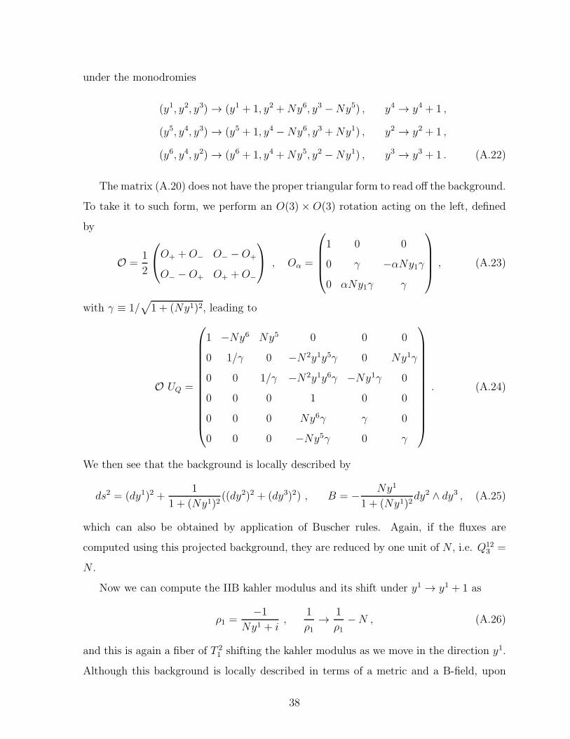
The matrix (A.20) does not have the proper triangular form to read off the background.

To take it to such form, we perform an O(3)× O(3) rotation acting on the left, defined

by

O =1

2

O+ +O− O− −O+

O− −O+ O+ +O−

, Oα =

1 0 0

0 γ −αNy1γ0 αNy1γ γ

, (A.23)

with γ ≡ 1/√

1 + (Ny1)2, leading to

O UQ =

1 −Ny6 Ny5 0 0 0

0 1/γ 0 −N2y1y5γ 0 Ny1γ

0 0 1/γ −N2y1y6γ −Ny1γ 0

0 0 0 1 0 0

0 0 0 Ny6γ γ 0

0 0 0 −Ny5γ 0 γ

. (A.24)

We then see that the background is locally described by

ds2 = (dy1)2 +1

1 + (Ny1)2((dy2)2 + (dy3)2) , B = − Ny1

1 + (Ny1)2dy2 ∧ dy3 , (A.25)

which can also be obtained by application of Buscher rules. Again, if the fluxes are

computed using this projected background, they are reduced by one unit of N , i.e. Q123 =

N .

Now we can compute the IIB kahler modulus and its shift under y1 → y1 + 1 as

ρ1 =−1

Ny1 + i,

1

ρ1→ 1

ρ1−N , (A.26)

and this is again a fiber of T 21 shifting the kahler modulus as we move in the direction y1.

Although this background is locally described in terms of a metric and a B-field, upon

38

going around a cycle y1 → y1 + 1, the metric and B-field mix through an S ∈ O(2, 2)

transformation OUQ(y1 + 1)S = OUQ(y

1), defined by

S =

1 0 0 0 0 0

0 γ(y1+1)γ(y1)

0 0 0 −Nγ(y1)γ(y1 + 1)

0 0 γ(y1+1)γ(y1)

0 Nγ(y1 + 1)γ(y1) 0

0 0 0 1 0 0

0 0 0 0 γ(y1)γ(y1+1)

0

0 0 0 0 0 γ(y1)γ(y1+1)

, (A.27)

where we have already projected to the base. The fact that under a cycle the metric and

B-field mix implies that this background is not globally well defined. However, as seen,

locally it is described by a metric and a B-field. Therefore, these backgrounds are said to

be locally geometric, but globally non-geometric.

R-flux

Finally, we apply the remaining T-duality in the direction y1 to obtain a background with

flux R123 = 3N where

UR =

1 0 0 0 0 0

0 1 0 0 0 0

0 0 1 0 0 0

0 −Ny6 Ny5 1 0 0

Ny6 0 −Ny4 0 1 0

−Ny5 Ny4 0 0 0 1

. (A.28)

This defines the one-forms

Γ4 = dy4 , Γ5 = dy5 , Γ6 = dy6 , (A.29)

Γ1 = dy1 −Ny6dy5 +Ny5dy6 ,

Γ2 = dy2 +Ny6dy4 −Ny4dy6 ,Γ3 = dy3 −Ny5dy4 +Ny4dy5 ,

39

and the monodromies

(y4, y2, y3)→ (y4 + 1, y2 +Ny6, y3 −Ny5) , y1 → y1 + 1 ,

(y5, y1, y3)→ (y5 + 1, y1 −Ny6, y3 +Ny4) , y2 → y2 + 1 ,

(y6, y1, y2)→ (y6 + 1, y1 +Ny5, y2 −Ny4) , y3 → y3 + 1 . (A.30)

The matrix UR reduces to the identity when projected to the base, and must then

be associated to a trivial torus with vanishing B-field. This can be understood if we

take into account that in every step of the T-duality procedure we project out the new

dual coordinates, and this successively reduces the flux by units of N . Since we started

from a background with H123 = 3N and performed three T-dualities, we have ended after

three successive projections with a background having R123 = 0. In summary, T-dualities

incorporate dual fluxes into the game which we are forced to project out if we want to

make contact with some string background geometry. In this example, this can be done

for H , ω and Q but not for R which then receives the name of locally non-geometric flux.

References

[1] M. Grana, “Flux compactifications in string theory: A Comprehensive review,”

Phys. Rept. 423 (2006) 91 [arXiv:hep-th/0509003]. M. R. Douglas and S. Kachru,

“Flux compactification,” Rev. Mod. Phys. 79 (2007) 733 [arXiv:hep-th/0610102];

R. Blumenhagen, B. Kors, D. Lust and S. Stieberger, “Four-dimensional String Com-

pactifications with D-Branes, Orientifolds and Fluxes,” Phys. Rept. 445, 1 (2007)

[arXiv:hep-th/0610327].

[2] H. Samtleben, “Lectures on Gauged Supergravity and Flux Compactifications,”

Class. Quant. Grav. 25, 214002 (2008) [arXiv:0808.4076 [hep-th]].

[3] J. Shelton, W. Taylor and B. Wecht, “Nongeometric flux compactifications,” JHEP

0510, 085 (2005) [arXiv:hep-th/0508133].

[4] G. Aldazabal, P. G. Camara, A. Font and L. E. Ibanez, “More dual fluxes and moduli

fixing,” JHEP 0605, 070 (2006) [arXiv:hep-th/0602089].

40

[5] G. Aldazabal, P. G. Camara and J. A. Rosabal, “Flux algebra, Bianchi identities

and Freed-Witten anomalies in F-theory compactifications,” Nucl. Phys. B 814, 21

(2009) [arXiv:0811.2900 [hep-th]].

[6] G. Aldazabal, E. Andres, P. G. Camara and M. Grana, “U-dual fluxes and General-

ized Geometry,” JHEP 1011 (2010) 083 [arXiv:1007.5509 [hep-th]].

[7] N. Hitchin, “Generalized Calabi-Yau manifolds,” Quart. J. Math. Oxford Ser. 54

(2003) 281 [arXiv:math/0209099].

[8] M. Gualtieri, “Generalized complex geometry,” arXiv:math/0401221.

[9] M. Grana, R. Minasian, M. Petrini and D. Waldram, “T-duality, Generalized Ge-

ometry and Non-Geometric Backgrounds,” JHEP 0904 (2009) 075 [arXiv:0807.4527

[hep-th]].

[10] S. Hellerman, J. McGreevy and B. Williams, “Geometric constructions of nongeo-

metric string theories,” JHEP 0401 (2004) 024 [arXiv:hep-th/0208174].

[11] A. Dabholkar and C. Hull, “Duality twists, orbifolds, and fluxes,” JHEP 0309 (2003)

054 [arXiv:hep-th/0210209].

[12] C. M. Hull, “A Geometry for non-geometric string backgrounds,” JHEP 0510 (2005)

065 [arXiv:hep-th/0406102].

[13] C. M. Hull and R. A. Reid-Edwards, “Flux compactifications of string theory on

twisted tori,” Fortsch. Phys. 57, 862 (2009) [arXiv:hep-th/0503114].

[14] A. Dabholkar and C. Hull, “Generalised T-duality and non-geometric backgrounds,”

JHEP 0605 (2006) 009 [arXiv:hep-th/0512005].

[15] C. M. Hull, “Doubled Geometry and T-Folds,” JHEP 0707 (2007) 080

[arXiv:hep-th/0605149].

[16] D. Berman, N. Copland and D. Thompson, “Background field equations for the

duality symmetric string,” Nucl. Phys. B 791 (2008) 175 [arXiv:0708.2267 [hep-th]]

41

[17] C. M. Hull and R. A. Reid-Edwards, “Gauge symmetry, T-duality and doubled ge-

ometry,” JHEP 0808 (2008) 043 [arXiv:0711.4818 [hep-th]].

[18] C. M. Hull and R. A. Reid-Edwards, “Non-geometric backgrounds, doubled geometry

and generalised T-duality,” JHEP 0909 (2009) 014 [arXiv:0902.4032 [hep-th]].

[19] D. Berman, M. J. Perry, “Generalized Geometry and M theory,” JHEP 1106 (2011)

074 [arXiv:1008.1763[hep-th]].

[20] D. S. Berman, H. Godazgar, M. J. Perry, “SO(5,5) duality in M-theory and general-

ized geometry,” Phys. Lett. B 700 (2011) 65 [arXiv:1103.5733[hep-th]].

[21] S. Kachru, M. B. Schulz, P. K. Tripathy and S. P. Trivedi, “New supersymmetric

string compactifications,” JHEP 0303 (2003) 061 [arXiv:hep-th/0211182].

[22] D. Andriot, M. Larfors, D. Lust and P. Patalong, “A ten-dimensional action for

non-geometric fluxes,” arXiv:1106.4015 [hep-th].

[23] C. Hull and B. Zwiebach, “Double Field Theory,” JHEP 0909 (2009) 099

[arXiv:0904.4664 [hep-th]].

[24] C. Hull and B. Zwiebach, “The Gauge algebra of double field theory and Courant

brackets,” JHEP 0909, 090 (2009) [arXiv:0908.1792 [hep-th]].

[25] O. Hohm, C. Hull and B. Zwiebach, “Background independent action for double field

theory,” JHEP 1007 (2010) 016 [arXiv:1003.5027 [hep-th]].

[26] O. Hohm, C. Hull and B. Zwiebach, “Generalized metric formulation of double field

theory,” JHEP 1008, 008 (2010) [arXiv:1006.4823 [hep-th]].

[27] O. Hohm and S. K. Kwak, “Massive Type II in Double Field Theory,”

arXiv:1108.4937 [hep-th].

[28] O. Hohm and S. K. Kwak, “Double Field Theory Formulation of Heterotic Strings,”

JHEP 1106 (2011) 096 [arXiv:1103.2136 [hep-th]].

42

[29] O. Hohm, S. K. Kwak and B. Zwiebach, “Double Field Theory of Type II Strings,”

arXiv:1107.0008 [hep-th].

[30] O. Hohm, S. K. Kwak and B. Zwiebach, “Unification of Type II Strings and T-

duality,” arXiv:1106.5452 [hep-th].

[31] C. Albertsson, S. H. Dai, P. W. Kao and F. L. Lin, “Double Field Theory for Double

D-branes,” arXiv:1107.0876 [hep-th].

[32] I. Jeon, K. Lee, J. Park, “Stringy differential geometry, beyond Riemann,” Phys.

Rev. D 84, 044022 (2011) [arXiv:1105.6294 [hep-th]].

[33] I. Jeon, K. Lee, J. Park, “Double field formulation of Yang-Mills theory,” Phys. Lett.

B 701 (2011) 260 [arXiv:1102.0419 [hep-th]].

[34] I. Jeon, K. Lee and J. H. Park, “Differential geometry with a projection: Application

to double field theory,” JHEP 1104 (2011) 014 [arXiv:1011.1324 [hep-th]].

[35] D. C. Thompson, “Duality Invariance: From M-theory to Double Field Theory,”

arXiv:1106.4036 [hep-th].

[36] O. Hohm and S. K. Kwak, “Frame-like Geometry of Double Field Theory,” J. Phys.

A 44 (2011) 085404 [arXiv:1011.4101 [hep-th]].

[37] S. K. Kwak, “Invariances and Equations of Motion in Double Field Theory,” JHEP

1010 (2010) 047 [arXiv:1008.2746 [hep-th]].

[38] J. Scherk and J. H. Schwarz, “How to Get Masses from Extra Dimensions,” Nucl.

Phys. B 153, 61 (1979).

[39] N. Kaloper and R. C. Myers, “The Odd story of massive supergravity,” JHEP 9905,

010 (1999) [arXiv:hep-th/9901045].

[40] J. Schon and M. Weidner, “Gauged N=4 supergravities,” JHEP 0605, 034 (2006)

[arXiv:hep-th/0602024].

43

[41] D. Andriot, “Heterotic string from a higher dimensional perspective,”

arXiv:1102.1434 [hep-th].

[42] G. Aldazabal, D. Marques, C. Nunez and J. A. Rosabal, “On Type IIB moduli stabi-

lization and N = 4, 8 supergravities,” Nucl. Phys. B 849, 80 (2011) [arXiv:1101.5954

[hep-th]].

[43] G. Dibitetto, A. Guarino and D. Roest, “How to halve maximal supergravity,” JHEP

1106, 030 (2011) [arXiv:1104.3587 [hep-th]].

[44] J. P. Derendinger, P. M. Petropoulos and N. Prezas, “Axionic symmetry gaugings

in N=4 supergravities and their higher-dimensional origin,” Nucl. Phys. B 785, 115

(2007) [arXiv:0705.0008 [hep-th]].

[45] W. Siegel, “Superspace duality in low-energy superstrings,” Phys.Rev. D48 (1993)

2826 [arXiv:hep-th/9305073]; W. Siegel, “Two vierbein formalism for string inspired

axionic gravity,” Phys.Rev. D47 (1993) 5453 [arXiv: hep-th/9302036].

[46] Andre Coimbra, Charles Strickland-Constable, Daniel Waldram, “Supergravity as

Generalised Geometry I: Type II Theories”, [arXiv:1107.1733 [hep-th]]

[47] G. Dall’Agata, G. Villadoro and F. Zwirner, “Type-IIA flux compactifications and

N=4 gauged supergravities,” JHEP 0908, 018 (2009) [arXiv:0906.0370 [hep-th]].

[48] T. Danckaert, J. Louis, D. Martinez-Pedrera, B. Spanjaard and H. Triendl, “The N=4

effective action of type IIA supergravity compactified on SU(2)-structure manifolds,”

arXiv:1104.5174 [hep-th].

[49] T. H. Buscher, “A Symmetry of the String Background Field Equations,” Phys. Lett.

B 194 (1987) 59.

[50] A. Giveon, M. Porrati and E. Rabinovici, “Target space duality in string theory,”

Phys. Rept. 244 (1994) 77 [arXiv:hep-th/9401139].

44

[51] G. Dall’Agata, N. Prezas, H. Samtleben and M. Trigiante, “Gauged Supergravities

from Twisted Doubled Tori and Non-Geometric String Backgrounds,” Nucl. Phys. B

799, 80 (2008) [arXiv:0712.1026 [hep-th]].

[52] D. Geissbuhler, “Double Field Theory and N=4 Gauged Supergravity,”

[arXiv:1109.4280 [hep-th]].

45