The effect of children on adult demands for health-risk reductions

T

Ta

b

c

a

ARRAA

JQQDI

KWVVHS

1

hmnhdfcpTch

iia

(

0d

Journal of Health Economics 29 (2010) 364–376

Contents lists available at ScienceDirect

Journal of Health Economics

journa l homepage: www.e lsev ier .com/ locate /econbase

he effect of children on adult demands for health-risk reductions

rudy Ann Camerona,∗, J.R. DeShazob, Erica H. Johnsonc

Department of Economics, 435 PLC, 1285, University of Oregon, Eugene, OR 97403-1285, United StatesSchool of Public Affairs, UCLA, 3250 Public Policy Building, Box 951656, Los Angeles, CA 90095-1656, United StatesSchool of Business Administration, Gonzaga University, 502 E. Boone, Spokane, WA 99258-0009, United States

r t i c l e i n f o

rticle history:eceived 21 June 2007eceived in revised form 2 December 2009ccepted 22 February 2010vailable online 1 March 2010

EL classification:515813

a b s t r a c t

We examine patterns in adults’ willingness to pay for health-risk reductions. We allow both their marginalutilities of income and their marginal disutilities from health risks to vary systematically with the struc-tures of their households. Demand by adults for programs which reduce their own health risks is foundto be influenced by (1) their parenthood status, (2) the numbers of children in different age bracketscurrently in their households, (3) the ages of the adults themselves, (4) the latency period before theywould fall ill, and (5) whether there will still be children in the household at that time. For younger adults,willingness to pay by parents is greater than for non-parents, and increases with each additional youngchild. For middle-aged adults, willingness to pay for corresponding risk reductions falls when teenagersare present and falls further with each additional teenager in the household.

18

eywords:TP for a microrisk reduction

alue of a statistical lifeSL

© 2010 Elsevier B.V. All rights reserved.

mceootwrnortfor which no theory yet exists.

Researchers have, of course, looked at many empirical aspects of

ealth riskstated preference survey

. Introduction

Parents can choose to invest in their own health and in theealth of their children. Jacobson (2000) developed a theoreticalodel of family-provided health to more fully explain the determi-

ants and dynamics of health investments in adults and children. Iner model, investments in each family member’s health are jointlyetermined by the allocation of income and time made by otheramily members. Subsequently, Bolin et al. (2001, 2002a,b) haveonsidered models of non-unitary household decision-making toredict inter-adult household allocations of investment in health.his growing and heterogeneous theoretical literature has yet to beonfronted with much empirical data on patterns in actual house-olds’ investments in health.

We begin to fill this gap in the literature by conducting an empir-cal assessment of the extent to which adults may change theirnvestments in their own health as a function of the numbers andges of children present in their households. While health invest-

∗ Corresponding author. Tel.: +1 541 346 1242; fax: +1 541 346 1243.E-mail addresses: [email protected] (T.A. Cameron), [email protected]

J.R. DeShazo), [email protected] (E.H. Johnson).

ci

waahm

167-6296/$ – see front matter © 2010 Elsevier B.V. All rights reserved.oi:10.1016/j.jhealeco.2010.02.005

ents may take many forms, we focus on investments that reduceurrent and future health risks from major illnesses. We providexamples of estimates, for specific types of adults in specific typesf households, of their willingness to pay (WTP) to reduce the riskf sick-time and lost life-years as a function of household struc-ure. The theoretical predictions of existing models are ambiguousith respect to the direction of adult investment in health-risk

eductions in the presence of children, so our empirical findings doot provide a head-to-head testing of existing theories. However,ur findings may contribute to future theoretical models by (1)evealing empirical regularities relevant to presently ambiguousheoretical predictions, and (2) highlighting patterns of behavior

hild health more generally, and at parents’ WTP for improvementsn the health of their children.1 Numerous studies also explore a

1 Some examples from the child health literature include Currie and Hotz (2004),ho find that a requirement of more education for day-care providers leads to fewer

ccidents involving the children in their care. Currie and Moretti (2003) find thatn increase in a mother’s education will, among other things, improve the health ofer infant. Currie and Neidell (2005) and Chay and Greenstone (2003) look at theeasurable negative effects of air pollution on infant health.

http://www.sciencedirect.com/science/journal/01676296

http://www.elsevier.com/locate/econbase

mailto:[email protected]



dx.doi.org/10.1016/j.jhealeco.2010.02.005

ealth

pimtroe“orhf

eticfretueuWsrcacagCta

ps

miWdtoaata2

oapnariee

p

wfipno

hffds(

apecatilEwafrw

r3etbph7

2

T.A. Cameron et al. / Journal of H

arent’s propensity to invest in their children’s health by reduc-ng the child’s risk of illness or death through improved access to

edications and better safety measures.2 Our work differs fromhese prior studies because we focus on adults’ WTP for health-riskeductions for themselves as a function of the presence of childrenf different ages. Perhaps Cropper and Sussman (1988) come clos-st to the issues addressed in this paper. They are concerned thatone must know the difference between the willingness to payf single people and those with dependents for a change in ownisk of death” (p. 259). Their research, however, considers WTP forealth-risk reductions—over the life-cycle and in the presence of

amilies—from a primarily theoretical perspective.Our analysis also contributes to the literature concerned with

stimation of the “value of a statistical life” (VSL).3 The main con-ribution of the present paper is to show how WTP of adults variesn the presence of children. This is important because some of theurrent literature focuses on whether it is appropriate to use someraction or multiple of a parent’s WTP to reduce their own healthisks as an estimate of their WTP to reduce their child’s risk. How-ver, if WTP is different for parents and non-parents, this “benefitsransfer” strategy may be inappropriate.4 We take advantage of anique data set drawn from an extensive existing stated prefer-nce survey described in Cameron and DeShazo (2009) that allowss to control for household structure and distinguish between theTP amounts for parents and non-parents. The stated preference

urvey elicits individuals’ demands for programs to reduce theirisks of a variety of specific major health threats. A methodologi-al advantage of our approach is that we are able to estimate thedult’s marginal utility of income as well as separate (and non-onstant) marginal disutilities of distinct future periods of illnessnd years of lost life. The contribution of this paper is to extend theeneral utility-theoretic choice modeling framework developed inameron and DeShazo (2009) to permit each of the marginal utili-ies in that paper to vary systematically with the gender of the adult
nd the nature of the household to which they belong.5
We provide the first empirical evidence of differences betweenarents and non-parents in willingness to pay to reduce the risk ofuffering a future time profile of adverse health states. We show

2 Among these, Thomas (1990) and Strauss and Thomas (1998) compare invest-ents in the health of children by mothers and fathers, but not parental investments

n their own health as our paper does. Liu et al. (2000) focus on Taiwanese mothers’TP to reduce the duration and severity of a cold for themselves and their chil-

ren, and Jenkins et al. (2001) focus on parents’ WTP for safer bicycle helmets forheir children. Dockins et al. (2002) and Scapecchi (2006) both address the questionf whether there are differences in WTP to reduce health risks for children versusdults. Hammitt and Haninger (2010) find WTP of adults is approximately twices large as for children using a stated preference survey on food-borne illness dueo pesticide residues. Other examples include Agee and Crocker (1996), Barron etl. (2004), Chenevier and LeLorier (2005), Dickie (2005), Dickie and Gerking (2006,007), Dickie and Messman (2004), Evans et al. (2009) and Maguire et al. (2004).3 A VSL is an average, scaled willingness to pay to reduce mortality risk. Estimates

f WTP by an individual are based on small reductions in mortality risks. Each avail-ble estimate typically corresponds to a different-sized risk reduction, so it is notossible to average the underlying unscaled WTP estimates. Thus, WTP estimateseed to be standardized on some common size of risk reduction before an aver-ge can be taken. The convention is to use the ratio of the marginal utility of a riskeduction to the marginal utility of income (a marginal rate of substitution), whichs equivalent to scaling all of these tiny risk reductions and their corresponding WTPstimates to a vastly larger 1.00 risk change. The average of a set of scaled-up WTPstimates is termed the “value of a statistical life”.4 We are grateful to an anonymous referee for suggesting that we include this

oint.5 Cameron and DeShazo (2009) develop and estimate a new structural model ofillingness to pay for microrisk reductions in health threats with different time pro-les of illness. The basic model in this earlier paper is for adults with homogeneousreferences, except for differences in age (nominal remaining life-years). There iso discussion of the effects of children, or any other aspects of household structure,n an individual’s demand for health risk reductions.

(citoecih

eiJtistsit

iepthi

o

Economics 29 (2010) 364–376 365

ow the WTP to reduce the risk of an adverse health profile differsor males and females according to the number of children in dif-erent age groups presently in the household, across single- versusual-income households, and as a function of whether children willtill be present in the household when the illness or injury strikesif there is a latency period involved).

We find that the number of children in different age groupsffects the adult’s marginal utility of income (which reflects com-eting demands on the household’s budget that may edge outxpenditures on the adult’s own health-risk reduction efforts). Con-urrently, we find evidence that the number of children in differentge categories affects the adult’s expected disutility from prospec-ive sick-time and prospective lost life-years—especially when thellness profile in question will affect the adult while there are stillikely to be children under the age of eighteen in the household.valuating the net effects on WTP, we find that for younger adults,illingness to pay by parents is greater than that by non-parents,

nd it increases with each additional young child. In contrast,or middle-aged adults, willingness to pay for corresponding riskeductions is lower when teenagers are present and falls furtherith each additional teenager in the household.

The next section briefly reviews the literature, emphasizingecent theoretical interest in the issues explored here. Section

outlines the survey method and the available data. Section 4xplains the structural indirect utility-based choice model we useo explain our respondents’ stated choices. This model forms theasis for our empirical specifications. Sections 5 and 6 discuss ourarameter estimates and illustrate their implications for WTP forealth-risk reductions under different circumstances, and Sectionconcludes.

. Literature on family structure and demand for health

Early theoretical models of the family, such as Becker and Tomes1976) and Leibowitz (1974), focus on parents’ investments in theirhildren rather than in themselves. However, parents’ investmentsn their own health may also represent indirect investments inhe well-being of an individual’s children. Jacobson (2000) devel-ped a theoretical model of family-provided health to more fullyxplain determinants of health investments in both adults andhildren.6 The health of a child is determined both by the fam-ly’s allocation of market goods to the child and by its allocation ofealth-denominated parental time to the child.

Consequently, we would expect that utility-maximizing parentsxplicitly consider the role that their own health plays in determin-ng the health and human capital development of their children.acobson also shows that parents need not be altruistic to invest inheir children’s health (although most parents probably are altru-stic toward their own children). Even parents who are entirelyelfish (e.g. those who do not appear to derive utility directly fromhe happiness of their child) will invest in the health of that childince failing to do so may have negative consequences for parents’ncomes (e.g. a sick child may reduce the time a parent may allocateo the labor market or to consumption activities).

This model by Jacobson (2000) shows that family members,nstead of equalizing health outcomes for each family member,qualize the marginal utility of lifetime health normalized by the
rice of health for that family member. Health influences income inwo separate ways—good health allows a parent to work and goodealth increases the parent’s wage rate. Since children require both
ncome and time from a parent, we would expect our empirical

6 Jacobson extends Grossman (1972) who models the individual as the producerf health.

3 ealth

admcaph

eJhvdTotsthhydrsd

psiobathcwaw

3

aomrvotvp

srsota

m

aoUIrtart

etsitdccsduiseAtwisan

fitrrpatstatclaid out and discussed, row by row, over the 16 preceding pages ofthe survey instrument.

Module 4 of the survey contains debriefing questions to per-mit cross-checks of the consistency of responses. Module 5 is

8 For more information on the survey instrument and the data, see the appen-dices which accompany Cameron and DeShazo (2009): Appendix A – Survey Design& Development, Appendix B – Stated Preference Quality Assurance and QualityControl Checks, Appendix C – Details of the Choice Set Design, Appendix D – TheKnowledge Networks Panel and Sample Selection Corrections, Appendix E – Model,

66 T.A. Cameron et al. / Journal of H

nalysis to show that the presence of children can affect parentalecisions in two ways. We expect children to increase a parent’sarginal utility of income since the additional costs of caring for

hildren will make the family budget tighter. Children also increaseparent’s marginal utility of healthy time, since time spent in allursuits becomes more valuable at the margin as the parent needsealthy time both to care for a child and to work.

Jacobson’s model assumes that both parents have common pref-rences, but she admits that this assumption may not be realistic.acobson’s model was extended by Bolin et al. (2001, 2002a,b) whoypothesize that a family’s investments in the health of the mother,ersus that of the father, can vary as a result of intra-householdecision-making and Nash bargaining between husband and wife.hough we cannot make ex ante theoretical predictions about theutcome of this Nash bargaining process for men and women,hese models illuminate the roles of several factors that may varyystematically across husbands and wives. Specifically, these fac-ors include labor market opportunity costs, the marginal utility ofealth improvement, and the marginal productivity of the parent’sealthy time for the child’s development.7 For our empirical anal-sis, this suggests that if a woman earns a lower income and/orerives greater marginal utility from additional income and faceselatively lower (and longer latency) health risks than her husband,he may be less willing to pay to reduce the risk of getting sick orying in the near term.

Another potential empirical implication arises from the inter-arent Nash bargaining allocation process. Bolin et al. (2002b)uggest that each parent’s control over family income may have anmpact upon their own health investments. Each parent’s degreef control over how income is allocated may depend in part uponoth the share of total household income earned by that parentnd the leverage generated from the threat of a possible exit fromhe household. (If the wife has her own income, for example, ausband’s threat of exit from the marriage has smaller financialonsequences for her.) This suggests for our empirical analysis thatomen who have independent incomes will be both more inclined,

nd more able, to invest in reducing their own health risks than willomen who depend entirely upon their husbands’ incomes.

. Available choice data

Existing market-based data are not adequate to infer individu-ls’ demands for risk reductions with respect to future time profilesf illness or injury. The revealed preference (RP) data which areost typically used concern tradeoffs between on-the-job fatality

isks and wages. This may be problematic because it excludes indi-iduals of interest for our analysis, such as stay-at-home mothersf young (or older) children. For groups like this who are not inhe labor market, stated preference (SP) data can be one of the fewiable sources of rich information concerning willingness to pay forrospective health-risk reductions.

We employ data from Cameron and DeShazo (2009) who usetated preference methods to elicit preferences for programs to
educe the risk of morbidity and mortality in a general populationample of adults in the United States. The survey was devel-ped carefully using 36 detailed in-person cognitive interviews,hree pretests and a large pilot study. Knowledge Networks, Inc.dministered the survey to 2439 of their panelists and achieved
7 The child’s health is also determined by efficiency parameters for both theother and father. See Eq. (22) on p. 622 of Jacobson (2000).

Eb

ipldhcicl

Economics 29 (2010) 364–376

respectable 79% response rate.8 The estimating sample consistsf choices by over 1800 individuals who are representative of the.S. population in terms of standard demographic characteristics.

n brief, the survey consists of five modules. The first module asksespondents to rate their subjective risks, from low to high, of con-racting each of a range of major illnesses or injuries. Individuals arelso asked to think about how lifestyle changes would reduce theirisks of these illnesses and how difficult it might be to implementhese lifestyle changes.

The second module in the survey is a detailed tutorial thatxplains the concept of an “illness profile” to be summarized inhe upcoming choice sets. An illness profile is a description of aequence of future health states associated with a major illness ornjury that the respondent may face over his or her remaining life-ime. The major and potentially life-threatening illnesses which areescribed in the survey are labeled as one of five specific types ofancer (breast cancer for women, prostate cancer for men, plus lungancer, colon cancer, and skin cancer), heart attack, heart disease,troke, respiratory illness, diabetes, traffic accident, or Alzheimer’sisease. An illness profile includes the years before the individ-al becomes sick (i.e. the latency period), illness-years while the

ndividual is sick, any recovered/remission years if the individualurvives the illness or injury, and lost life-years if the individual diesarlier than he would have in the absence of the illness or injury.fter the tutorial about illness profiles, the individual is informed

hat he or she might soon be able to purchase new programs thatould reduce the risks of experiencing certain illness profiles. Each

llness-related risk-reduction program described in the survey con-ists of an annual diagnostic blood test plus possible drug therapiesnd/or lifestyle changes, available at a specified overall cost that isot covered by insurance.9

The third, and key, module of each survey involves a set ofve different three-alternative conjoint choice experiments wherehe individual is asked to choose one of the two possible health-isk-reducing programs or a status quo alternative. Each programeduces the individual’s risk of experiencing a specific illnessrofile. The illness profile is described in terms of its baseline prob-bility, age at onset, duration, severity of symptoms and type ofreatment, and eventual outcome (recovery or death). Each corre-ponding risk-reduction program is defined in terms of the extento which it can be expected to reduce this risk, as well as its monthlynd annual cost. Fig. 1 provides one randomized example of theype of a stated choice scenario posed to respondents. This firsthoice set summary was presented only after its contents had been

stimation and Alternative Analyses, and Appendix F – Estimating Sample Code-ook.9 Early drafts of the survey made an effort to spell out that the quoted costs were

ntended to capture all of the monetized opportunity costs of participating in therogram, but this additional material had to be cut to keep the survey within its

ength restrictions. An anonymous referee has suggested that we consider respon-ents’ subjective perceptions about how easy it would be to improve their healthabits. Respondents who would find it harder to make life-style changes have largeroefficients on their net income variable, which could be taking up the effect of whats instead just a larger value of perceived net income (i.e. smaller perceived programosts). Thus respondents do not, on average, appear to be imputing significantlyarger full costs than are stated in the choice scenarios.

T.A. Cameron et al. / Journal of Health Economics 29 (2010) 364–376 367

rando

cdri

rppsoootitprtot

i

avaaattwtrei

adprdpFiVauE

pvs

Fig. 1. One example of a

ollected separately from our survey and contains detailed socio-emographic data for the individual and the household, as well asesponses to a battery of health-related questions (including anyllnesses the individual has already faced).

Extensive robustness and validity checks of the individuals’esponses have been conducted to evaluate most of the commonroblems which may affect SP analyses.10 These include risk com-rehension verification where individuals are asked to rank theizes of stated risk reductions, checks on the subjective complexityf each choice set where individuals are asked to rate the difficultyf the choice sets, analyzed in Duquette et al. (2009), and the rec-mmended “cheap talk” reminder so that individuals are carefulo consider their budget constraints and not overstate their will-ngness to pay.11 Individuals are specifically instructed to assumehat each choice set is independent of the other choice sets. Inreliminary simple ad hoc specifications, respondents’ choices are
eadily demonstrated to be markedly sensitive to the changes inhe scope of the central attributes of these choice sets (i.e. the costf the program and the size of the risk reduction). Although sys-ematic sample selection effects are very minor, they are carefully
10 For the details, see Appendix B – Stated Preference Quality Assurance and Qual-ty Control Checks, which accompanies Cameron and DeShazo (2009).11 A number of individuals and/or choice sets were dropped from the analysisccording to three exclusion criteria. Exclusion for risk comprehension was acti-ated if the respondent could not successfully rank the sizes of the risk reductionsssociated with two risk mitigation programs. The 1629 choices by these individu-ls were excluded from the analysis. Exclusion for outright scenario rejection wasctivated for choices where the respondent chose the “neither program” alterna-ive and in the follow-up question which probed why, reported “I did not believehe programs would work” as the only reason for this choice. A total of 2236 choicesere excluded due to scenario rejection. A further 332 choices were excluded due

o a minor error in the randomized design for these choice sets which led to theesult that suffering from the illness in question would extend the respondent’s lifexpectancy by a small amount. While this could conceivably happen, we had notntended this to occur, so we dropped these choices.

riattsatmdat

tbKC

mized choice scenario.

ssessed and controlled for.12 Finally, Cameron and DeShazo (2009)emonstrate that the WTP implications from a basic model—withreferences that are assumed to be homogeneous except withespect to age, and for the VSL-type health risk consisting of suddeneath in the current period—are entirely consistent with contem-orary government assumptions about the value of a statistical life.or a 45-year-old with $42,000 in household income, and assum-ng a 5% discount rate, the model’s WTP estimate corresponds to aSL of roughly $5.4 million with a 90% range between $3.6 millionnd $7.4 million. This interval captures the VSL estimates actuallysed by both the U.S. Department of Transportation and the U.S.PA during the same time period.

The variables from the survey which are pertinent to theresent empirical analysis are summarized in Table 1. Theseariables include attributes of the different illness profiles pre-ented to respondents (latency, present discounted sick-years,ecovered/post-illness-years, and lost life-years). The list alsoncludes attributes of the proposed risk-reduction programs whichre described as reducing the individual’s chance of suffering fromhese adverse health states (including the cost of the program andhe size of the risk reduction). The household’s budget and thetructure of earnings are captured by household income data andn indicator for the presence of more than one income-earner inhe household. The respondent’s gender is also employed in our

odels. The illness profile information, combined with householdemographic information including the respondent’s own currentge and data on the numbers and ages of children currently inhe household, allows us also to determine whether the onset of

12 A formal sample selection model has been developed for this sample, relativeo the roughly 525,000 initial random-digit dialed recruiting contacts attemptedy Knowledge Networks in building their consumer panel. See Appendix D – Thenowledge Networks Panel and Sample Selection Corrections, which accompaniesameron and DeShazo (2009).

368 T.A. Cameron et al. / Journal of Health Economics 29 (2010) 364–376

Table 1Descriptive statistics (assumes 5% discount rate) (7520 choice sets; 22,560 alternatives; 15,040 illness profiles; 1801 individuals).

Variable Description Mean Std. Dev. Min Max

Illness profileslatencyj

iTime until onset (years) 19.58 12.02 1 60

pdviji

Present discounted sick-years 2.21 2.51 0 16.3pdvrj

iPresent discounted recovered-years 0.474 1.36 0 15.9

pdvlji

Present discounted lost life-years 2.57 2.93 0 17.81(child at onsetj

i) =1 if current child < 18 at illness onset .02859

Risk-reduction programscj

iMonthly cost $29.87 28.71 2 140

�˘ji

Risk change −.00341 .00167 −.006 −.001

Respondent characteristicsYi Income 2002 $US $50,771 33,966 5000 150,000agei0 Age in years at time of survey 50.30 15.21 25 931(femalei) =1 if female, =0 if male 0.5131(marriedi) =1 if married, =0 if unmarried 0.688nkids01i # children aged 0–1 years in household .0161 .1352 0 2nkids25i # children aged 2–5 years in household .1254 .3880 0 3nkids612i # children aged 6–12 years in household .2143 .5737 0 5nkids1317i # children aged 13–17 years in household .1575 .4563 0 31(dualinci) =1 if two incomes in household .6356

benefi

aar

4

ciDlcaithstits

w(taswtb

P

Io(

a

gte

P

Tad

�

Ons

nmcfompare sick or dead.14 They are also modeled as expecting to receiveroughly their current level of real income for as long as they live.15

Since each illness profile spans the rest of each person’s life,we define the discount rate as r and let ıt = (1 + r)−t.16 The present

14 Page 21 of the survey instrument specifies that the respondent “would need topay for, and participate in, a program for the next [x] years to get its benefits,” wherethe value of [x] reflects the respondents current age and corresponding nominal lifeexpectancy. Test subjects believed they would not have to pay for the tests while

Illness profile/respondent interactions1(neverj

i) =1 if the individual states that “the program will never

bendiff ji

The individual’s minimum overestimate of the latency

dverse health states in a given illness profile will occur when therere likely to be children still under the age of 18 present in theespondent’s household.

. A random utility choice model

We use a specification that generalizes the utility-theoretichoice model presented in Cameron and DeShazo (2009) by allow-ng for heterogeneity due to household structure. Cameron andeShazo (2009) establish that stated choices in this general popu-

ation sample appear to be best explained by a model that involvesonstrained discounted expected utility. Utility is modeled as beingdditively separable in two components, the first pertaining toncome and costs, and the second pertaining to health state dura-ions. Thus the marginal utility of income does not depend uponealth states, and the marginal utility of present discounted healthtates does not depend upon net income. In our basic specifications,hese restrictions are not rejected by the data. To permit systemat-cally varying degrees of diminishing marginal utility with respecto net income, indirect utility is modeled as quadratic, rather thanimply linear, in net income.

As a sketch of the basic model, we will consider just a pair-ise choice between Program A and the status quo alternative

N).13 First consider what happens if individual i chooses the sta-us quo alternative. Let ˘NS

ibe the probability of suffering a given

dverse health profile—i.e. getting sick (S) and experiencing thepecified series of health states over time. Under the status quoith no risk-reducing program, discounted expected utility, with

he expectation taken across getting sick or staying healthy (H), cane denoted as:

N NS NS NS NH
DV(E[Vi ]) = PDV(˘i Vi + (1 − ˘i )Vi )
f individual i chooses Program A, however, then the probabilityf suffering the adverse health profile is lower. Let ˘AS

ibe the

reduced) probability of suffering the adverse health profile if Pro-

13 The model for a three-way discrete choice, between two alternative programsnd the status quo, is analogous.

td

eiwni

a

t me” 0.385 .4865−5.95 11.08 −59 29

ram A is chosen. Then �˘ASi

= ˘ASi

− ˘NSi

< 0 is the risk changeo be achieved by participating in Program A. We can write thexpected utility from choosing Program A as:

DV(E[VAi ]) = PDV(˘AS

i VASi + (1 − ˘AS

i )VAHi )

hen the difference in the present discounted expected utility whenn individual chooses Program A instead of the status quo can beenoted by:

PDV [E(VAi )] = PDV [E(VA

i )] − PDV [E(VNi )] (1)

ur empirical specification is based on the assumption that a ratio-al individual will choose Program A if �PDV [E(VA

i)] > 0, and the

tatus quo otherwise.Operationally, the sequence of health states making up the ill-

ess profile to be addressed by Program A is captured by a set ofutually exclusive and exhaustive (0, 1) indicator variables asso-

iated with each future time period t. We use the indicator 1(preAit

)or pre-illness-years, 1(illA

it) for illness-years, 1(rcvA

it) for recovered

r post-illness-years, and 1(lylAit

) for life-years lost. Individuals areodeled as expecting to pay the annual cost of the risk-reduction

rogram only during pre-illness and recovered years, but not if they

hey were actually sick with the illness in question, and certainly not after they wereead, so we imposed this assumption in our empirical models.15 It proved impossible, within survey length constraints, to elicit comprehensivexpectations about the time profile of future income, with and without each type ofllness. We assume that the individual believes that disability insurance and savings

ill make up roughly their current real income during illness, but they will receiveo regular income after their death. There is no information about planned bequests

n our data.16 Illness profiles were tailored in advance to each panelist’s gender and currentge. Due to the advance preparation of randomized illness profiles, we could ensure

ealth

dipida∑st

tepcn˘atA˘dq

�

I(�f(bacm

bidGt

ta

tot

a

wa

(ddrssmic

jrte

c

wtsr

E

sabp

W

Mc“dap

tdit

p

haso


iscounted number of years making up the remainder of thendividual’s (cumulative) nominal life expectancy, Ti, is given bydvcA

t =∑Ti

t=1ıt . With the help of the four different health-statendicator variables, future time periods in each health state areiscounted and summed from t = 1 to Ti and the resulting termsre denoted by pdveA

i=

∑ıt1(preA

it), pdviA

i=

∑ıt1(illA

it), pdvrA

i=

ıt1(rcvAit

) and pdvlAi

=∑

ıt1(lylAit

). Since the different healthtates exhaust the individual’s nominal life expectancy, it will behe case that pdveA

i+ pdviA

i+ pdvrA

i+ pdvlA

i= pdvcA

i.

To accommodate the assumption that each individual expectso pay program costs only during the pre-illness or recov-red/remission periods, we define pdvpA

i= pdveA

i+ pdvrA

i, the

resent discounted time over which payments must be made. Thisan be interpreted as the discounted duration of program costs. Theotation can be simplified further when we define ctermA

i= [(1 −

ASi

)pdvcAi

+ ˘ASi

pdvpAi], where ctermA

ican be explained intuitively

s the expected number of present discounted years over whichhe program costs will be paid if the individual chooses Program. For simplicity, we also define ytermA

i= [−pdvcA

i+ ˘AS

ipdviAS

i+

NSi

pdvlAi].17 The generic expected utility-difference in Eq. (1) that

rives the individual’s choice between Program A and the statusuo can then be defined as18:

PDV [E(VAi )] = ˇ0{(Yi − cA

i )ctermAi + YiytermA

i }

+ ˇ1{(Yi − cAi )

2ctermA

i + Y2i ytermA

i }

+ ˛1{�˘ASi pdviAi } + ˛2{�˘AS

i pdvrAi }

+ ˛3{�˘ASi pdvlAi } + εA

i (2)

n what follows, we will use the shorthand notation of ptermAi

the “profile” term) to refer generically to the full set of terms inPDV [E(VA

i)] which involve discounted time in each of the three

uture adverse health states: illness (pdvi), recovery/remissionpdvr), and lost life-years (pdvl).19 In Eq. (2), the five terms in curlyraces can be constructed from the data, given specific assumptionsbout the discount rate. The unknown indirect utility parametersan then be estimated using McFadden’s conditional logit choiceodel.20

Estimates of WTP for a specified risk reduction can be derivedy recombining the estimated parameters and the data employed

n the choice model in Eq. (2). The appropriate utility-theoreticemand construct is a so-called “option price.” In the sense ofraham (1981), the option price for a risk-reduction program is

he maximum common certain payment that makes the individual

hat gender-specific illnesses were correctly assigned and that no respondent wassked to consider an illness that would begin prior to their current age.17 This ytermA

ivariable does not have a similarly straightforward intuitive explana-

ion; we use this abbreviation merely to simplify the notation below. The complexityf this term stems from the assumed pattern of income and program costs acrosshe individual’s probabilistic future health states.18 There will be an analogous term for the utility difference between Program Bnd the status quo in our three-alternative model.19 We note that since health status and net income are assumed to be constantithin each health state interval, one can freely reverse the order of the discounting

nd expectations operations.20 In this paper, we assume a common discount rate of 5%. Cameron and DeShazo2009) explore the consequences of assuming either a 3% discount rate or a 7%iscount rate. Work in progress also involves the estimation of individual-specificiscount rates simultaneously with these stated choices concerning health riskeduction programs, using additional data on intertemporal choices by a separateample of respondents from the same population. Preliminary results, however,uggest that the 5% across-the-board discount rate assumption produces a maxi-ized value of the log-likelihood function that is almost 80 points higher than the

ndividual-specific fitted discount rates which are a function of sociodemographicharacteristics of each individual.

lfatn

p

Fsdww˛

mt

u

Economics 29 (2010) 364–376 369

ust indifferent between paying for the program (and enjoying theisk reduction) and not paying for the program (and not enjoyinghe risk reduction).21 The annual option price cA

ithat makes the

xpression in Eq. (2) exactly zero can be calculated as:

ˆAi = Yi − f −1

((ˇ0 + ˇ1Yi)ytermA

i+ ptermA

i+ εA

i

−(ˇ0 + ˇ1Yi)ctermAi

)(3)

here f (Y) = (ˇ0 + ˇ1Yi)Yi = ˇ0Yi + ˇ1Y2i

, so that f−1() is the solu-ion to a quadratic form. The expected present value of thistream of annual payments must be calculated over the individual’semaining nominal lifespan:

[PV(cAi )] = ctermA

i [cAi ] (4)

To convert this expected present value option price into a mea-ure of the WTP for a microrisk reduction, one can normalizerbitrarily on a one-in-one-million risk change by dividing this WTPy the absolute size of the risk reduction and scaling by .000001 toroduce:

TP = E[PV(cAi

)]

�˘ASi

× 0.000001 (5)

ultiplying by 1.0 instead of 0.000001 would produce a numberomparable to the value of a statistical life (VSL) for the appropriatesudden death now” illness profile. Note that this WTP constructepends fundamentally on the individual’s age and income, as wells on the illness profile in question and the estimated indirect utilityarameters in Eq. (2). It is not a simple constant.

As described in Cameron and DeShazo (2009), the data suggesthat the basic, homogeneous-preferences model given in Eq. (2) isominated by a specification that is not merely linear in the terms

nvolving present discounted health-state years. We can rewritehe terms in Eq. (2) that involve the ˛ coefficients as:

termji= �˘jS

i[˛1pdvij

i+ ˛2pdvrj

i+ ˛3pdvlj

i], j = A, B (6)

However, this simple linear specification in our discountedealth state variables does not explain respondents’ stated choicess well as an alternative model that employs shifted logarithms,uch as log(pdvi + 1), etc. We invoke then the well-known abilityf the translog functional form to serve as a flexible second-orderocal approximation to any arbitrary function. If we start from aorm that is fully translog (including all squares and pairwise inter-ction terms for the three shifted log terms), and then retain onlyhose terms where the ˛ coefficients are robustly statistically sig-ificantly different from zero, ptermj

ibecomes:

termji

= �˘jSi

[˛1 log(pdviji+ 1) + ˛2 log(pdvrj

i+ 1)

+ ˛3 log(pdvlji+ 1) + ˛4{log(pdvlj

i+ 1)}2

+ ˛5{log(pdviji+ 1) log(pdvlj

i+ 1)}] (7)

inally, because the opportunity for longer durations in each healthtate is unavoidably correlated with the youth of the respon-ent, these ˛ coefficients must be allowed to differ systematicallyith the respondent’s current age wherever this generalization isarranted by the data. This leads to a model where ˛3 = ˛30 +
31agei + ˛32age2
i, and analogously for ˛4 and ˛5.

This quadratic-in-age systematic variation in parameters per-its non-constant age profiles for the model’s WTP estimates. For

he special case of a VSL-type illness profile consisting of “sudden

21 This notion of an option price differs from the sense in which is customarilysed in the finance literature.

3 ealth Economics 29 (2010) 364–376

ddom

tTwlpaehugidfoa

facwmtnv

5

img(Saaedbitaftms

nv

esrtiait

f

Table 2Final model (n = 1801 individuals, 7520 choices, 22,560 alternatives).

Full model

Linear net income term(ˇ00 × 105)[linear net income term] 4.663 (6.21)***

. . . × 1(femalei) 6.241 (5.28)***

. . . × 1(femalei) × nkids612i −2.266 (2.02)**

. . . × nkids1317i 2.143 (2.31)**

. . . × 1(femalei) × 1(dualinci) −0.165 (1.59)

Quadratic net income term(ˇ10 × 109)[quadratic net income term] 0. . . × 1(femalei) −.2835 (3.89)***

. . . × nkids01i −.762 (2.41)**

Sick-years terms(˛10)�˘jS

ilog(pdvij

i+ 1) −70.71 (5.22)***

. . . × 1(femalei) 28.4 (2.17)**

. . . × nkids25i 103.8 (3.80)***

. . . × 1(femalei) × nkids25i −68.52 (2.11)**

. . . × 1(child at onsetji) −116 (3.07)***

Recovered-years terms(˛20)�˘jS

ilog(pdvrj

i+ 1) −58.54 (5.78)***

Lost life-years terms(˛30)�˘jS

ilog(pdvlj

i+ 1) −600.2 (3.28)***

. . . × 1(femalei) 22.75 (2.02)**

. . . × 1(marriedi) −34.54 (3.09)***

. . . × nkids25i −33.66 (1.98)**

. . . × nkids1317i 26.22 (2.24)**

(˛31)agei0 · �˘jSi

log(pdvlji+ 1) 33.66 (4.67)***

(˛32)age2i0

· �˘jSi

log(pdvlji+ 1) −0.285 (4.23)***

Lost life-years squared terms

(˛40)�˘jSi

[log(pdvlji+ 1)]

2212.4 (2.35)***

(˛41)agei0 · �˘jSi

[log(pdvlji+ 1)]

2 −13.12 (3.63)***

(˛42)age2i0

· �˘jSi

[log(pdvlji+ 1)]

20.113 (3.28)***

Sick-years, lost life-years interaction terms(˛50)�˘jS

i[log(pdvij

i+ 1)] · [log(pdvlj

i+ 1)] −44.59 (4.18)***

. . . × 1(child at onsetji) 555.5 (2.39)**

(˛51)agei0 · �˘jSi

[log(pdviji+ 1)] · [log(pdvlj

i+ 1)] 0

. . . × 1(child at onsetji) −22.4 (2.17)**

(˛52)age2i0

· �˘jSi


i+ 1)] 0

. . . × 1(child at onsetji) .2457 (2.20)**

Nuisance parametersShift if respondent believes “will never benefit”

(ˇ101 × 1019)[second income term] × 1(neverj

i) 0.743 (2.97)***

(˛101)�˘jSi

log(pdviji+ 1) × 1(neverj

i) 206.8 (3.82)***

(˛401)�˘jSi

[log(pdvlji+ 1)]

2 × 1(neverji) 413.9 (4.69)***

(˛411)agei0 · �˘jSi

[log(pdvlji+ 1)]

2 × 1(neverji) −5.567 (3.93)***

(˛501)�˘jSi


i+ 1)] × 1(neverj

i) −355.4 (3.84)***

(˛521)age2i0

�˘jSi


i+ 1)] × 1(neverj

i) 0.08 (3.52)***


eath in the current period,” the ptermjispecification in Eq. (7) pro-

uces the typical inverted U-shape for a plot of WTP as a functionf the respondent’s current age, with higher WTP values duringiddle age and lower values for younger and older respondents.22

A respondent’s subjective perceptions do not always matchhe assumptions embedded in the illness profile descriptions.hus Cameron et al. (2009) construct a variable called bendiff j

i,

hich approximates the individual’s over- or under-estimate of theatency of each health problem addressed by each risk-reductionrogram. After each stated choice in the survey, respondents aresked when they, personally, believe they would begin to experi-nce the benefits of each of the two risk-reduction programs theyave just considered. A separate indicator variable, 1(neverj

i), is also

sed—for those programs where the individual states that “the pro-ram will never benefit me.” If 1(neverj

i) = 0 and bendiff j

i= 0, the

ndividual is deemed to have accepted the illness profile as it isescribed in the scenario. In the present paper, we use the modelrom Cameron et al. (2009) that includes 1(neverj

i) and bendiff j

ias

ur “baseline” model and focus on the consequences of introducingdditional interaction terms.

There may be important sources of unobserved heterogeneityor which we are unable to control, such as future health insur-nce coverage and expected additional children. In addition, it is ofourse relevant that child-bearing decisions are jointly endogenousith an individual’s expected life-cycle investment in health-riskitigation. However, at the point when our respondents are asked

o consider new health-risk-reduction programs in the survey, theumber of children presently in the household can at least beiewed as a predetermined variable.

. Empirical estimation

Recall that WTP for the health-risk reductions in our models determined by the ratio of marginal (dis)utility of risk to the

arginal utility of income. Our first set of models describes howender, age and household structure affect an individual’s marginaldis)utility of risk and marginal utility of income respectively.econd, with these marginal utility estimates in hand, we evalu-te the net effects of gender, age and household structure on andult’s willingness to pay to reduce risks to their own health. Ourxploration coalesced around a set of five increasingly general con-itional logit random utility models (RUMs).23 These models areased on an initial specification that is quadratic in discounted net

ncome and employs age-varying translog-like transformations oferms in the numbers of sick-years, recovered (post-illness) yearsnd lost life-years which make up each illness profile. Our pre-
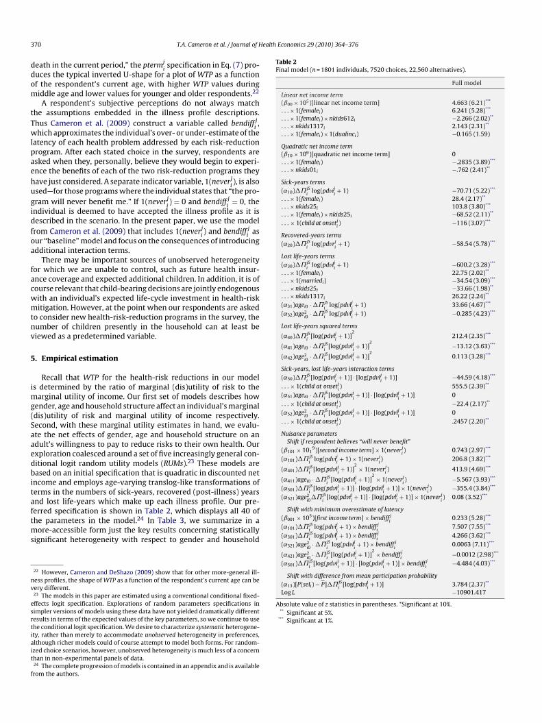
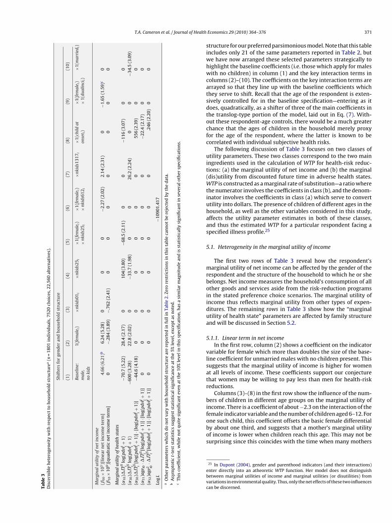
erred specification is shown in Table 2, which displays all 40 ofhe parameters in the model.24 In Table 3, we summarize in a
ore-accessible form just the key results concerning statisticallyignificant heterogeneity with respect to gender and household

22 However, Cameron and DeShazo (2009) show that for other more-general ill-ess profiles, the shape of WTP as a function of the respondent’s current age can beery different.23 The models in this paper are estimated using a conventional conditional fixed-ffects logit specification. Explorations of random parameters specifications inimpler versions of models using these data have not yielded dramatically differentesults in terms of the expected values of the key parameters, so we continue to usehe conditional logit specification. We desire to characterize systematic heterogene-ty, rather than merely to accommodate unobserved heterogeneity in preferences,lthough richer models could of course attempt to model both forms. For random-zed choice scenarios, however, unobserved heterogeneity is much less of a concernhan in non-experimental panels of data.24 The complete progression of models is contained in an appendix and is availablerom the authors.

Shift with minimum overestimate of latency(ˇ001 × 105)[first income term] × bendiff j

i0.233 (5.28)***

(˛101)�˘jSi

log(pdviji+ 1) × bendiff j

i7.507 (7.55)***

(˛301)�˘jSi

log(pdvlji+ 1) × bendiff j

i4.266 (3.62)***

(˛321)age2i0

· �˘jSi

log(pdvlji+ 1) × bendiff j

i0.0063 (7.11)***

(˛421)age2i0

· �˘jSi

[log(pdvlji+ 1)]

2 × bendiff ji

−0.0012 (2.98)***

(˛501)�˘jSi


i+ 1)] × bendiff j

i−4.484 (4.03)***

Shift with difference from mean participation probability(˛13)[P(seli) − P]�˘jS

i[log(pdvij

i+ 1)] 3.784 (2.37)**

Log L −10901.417

Absolute value of z statistics in parentheses. *Significant at 10%.** Significant at 5%.

*** Significant at 1%.

T.A. Cameron et al. / Journal of Health

Tab

le3

Dis

cern

ible

het

erog

enei

tyw

ith

resp

ect

toh

ouse

hol

dst

ruct

ure

a(n

=18

01in

div

idu

als,

7520

choi

ces,

22,5

60al

tern

ativ

es).

Shif

ters

for

gen

der

and

hou

seh

old

stru

ctu

re

(1)

(2)

(3)

(4)

(5)

(6)

(7)

(8)

(9)

(10)

Base

line:

mal

e,no

kids

1(fe

mal

e i)

×nki

ds01

i×n

kids

25i

×1(f

emal

e i)

×nk

ids2

5 i×1

(fem

ale i

)×

nkid

s612

i

×nki

ds13

17i

×1(c

hild

aton

set i

)×1

(fem

ale i

)×

1(du

alin

cii)

×1(m

arri

edi)

Mar

gina

luti

lity

ofne

tin

com

e(ˇ

00×

105)[

lin

ear

net

inco

me

term

]4.

66(6

.21)

b6.

24(5

.28)

00

0−2

.27

(2.0

2)2.

14(2

.31)

0−1

.65

(1.5

9)c

0(ˇ

10×

109)[

quad

rati

cn

etin

com

ete

rm]

0−.

284

(3.8

9)−.

762

(2.4

1)0

00

00

00

Mar

gina

luti

lity

ofhe

alth

stat

es(˛

10)�

˘jS i

log(

pdvi

j i+

1)−7

0.7

(5.2

2)28

.4(2

.17)

010

4(3

.80)

−68.

5(2

.11)

00

−116

(3.0

7)0

0(˛

30)�

˘jS i

log(

pdvl

j i+

1)−6

00(3

.28)

22.8

(2.0

2)0

−33.

7(1

.98)

00

26.2

(2.2

4)0

0−3

4.5

(3.0

9)(˛

50)�

˘jS i

[log

(pdvi

j i+

1)]·

[log

(pdvl

j i+

1)]

−44.

6(4

.18)

00

00

00

556

(2.3

9)0

0(˛

51)a

gei0

·�˘

jS i[l

og(p

dvi

j i+

1)]·

[log

(pdvl

j i+

1)]

00

00

00

0−2

2.4

(2.1

7)0

0(˛

52)a

ge2 i0

·�˘

jS i[l

og(p

dvi

j i+

1)]·

[log

(pdvl

j i+

1)]

00

00

00

0.2

46(2

.20)

00

Log

L−1

0901

.417

aO

ther

par

amet

ers

wh

ich

do

not

vary

wit

hh

ouse

hol

dst

ruct

ure

are

rep

orte

din

full

inTa

ble

2.Ze

rore

stri

ctio

ns

inth

ista

ble

can

not

bere

ject

edby

the

dat

a.b

Asy

mp

toti

ct-

test

stat

isti

cssu

gges

tst

atis

tica

lsig

nifi

can

ceat

the

5%le

vel,

exce

pt

asn

oted

.c

This

coef

fici

ent,

wh

ile

not

quit

esi

gnifi

can

tev

enat

the

10%

leve

lin

this

spec

ifica

tion

,has

asi

mil

arm

agn

itu

de

and

isst

atis

tica

lly

sign

ifica

nt

inse

vera

loth

ersp

ecifi

cati

ons.

siwhwcatsdtocfc

uit(Wtiuhaas

5

mrboiidua

5

vlsatr

bifobos

ebvc

Economics 29 (2010) 364–376 371

tructure for our preferred parsimonious model. Note that this tablencludes only 21 of the same parameters reported in Table 2, but

e have now arranged these selected parameters strategically toighlight the baseline coefficients (i.e. those which apply for malesith no children) in column (1) and the key interaction terms in

olumns (2)–(10). The coefficients on the key interaction terms arerrayed so that they line up with the baseline coefficients whichhey serve to shift. Recall that the age of the respondent is exten-ively controlled for in the baseline specification—entering as itoes, quadratically, as a shifter of three of the main coefficients inhe translog-type portion of the model, laid out in Eq. (7). With-ut these respondent-age controls, there would be a much greaterhance that the ages of children in the household merely proxyor the age of the respondent, where the latter is known to beorrelated with individual subjective health risks.

The following discussion of Table 3 focuses on two classes oftility parameters. These two classes correspond to the two main

ngredients used in the calculation of WTP for health-risk reduc-ions: (a) the marginal utility of net income and (b) the marginaldis)utility from discounted future time in adverse health states.

TP is constructed as a marginal rate of substitution—a ratio wherehe numerator involves the coefficients in class (b), and the denom-nator involves the coefficients in class (a) which serve to converttility into dollars. The presence of children of different ages in theousehold, as well as the other variables considered in this study,ffects the utility parameter estimates in both of these classes,nd thus the estimated WTP for a particular respondent facing apecified illness profile.25

.1. Heterogeneity in the marginal utility of income

The first two rows of Table 3 reveal how the respondent’sarginal utility of net income can be affected by the gender of the

espondent and the structure of the household to which he or sheelongs. Net income measures the household’s consumption of allther goods and services aside from the risk-reduction programsn the stated preference choice scenarios. The marginal utility ofncome thus reflects marginal utility from other types of expen-itures. The remaining rows in Table 3 show how the “marginaltility of health state” parameters are affected by family structurend will be discussed in Section 5.2.

.1.1. Linear term in net incomeIn the first row, column (2) shows a coefficient on the indicator

ariable for female which more than doubles the size of the base-ine coefficient for unmarried males with no children present. Thisuggests that the marginal utility of income is higher for woment all levels of income. These coefficients support our conjecturehat women may be willing to pay less than men for health-riskeductions.

Columns (3)–(8) in the first row show the influence of the num-ers of children in different age groups on the marginal utility of

ncome. There is a coefficient of about −2.3 on the interaction of theemale indicator variable and the number of children aged 6–12. For
ne such child, this coefficient offsets the basic female differentialy about one third, and suggests that a mother’s marginal utilityf income is lower when children reach this age. This may not beurprising since this coincides with the time when many mothers
25 In Dupont (2004), gender and parenthood indicators (and their interactions)nter directly into an atheoretic WTP function. Her model does not distinguishetween marginal utilities of income and marginal utilities (or disutilities) fromariations in environmental quality. Thus, only the net effects of these two influencesan be discerned.

3 ealth

rilboipitwa

iabis(s

5

otddiiwmgttcm

tmHqff

5

oocu

n

sis

tcne

5

ddaft

5

ei2sfibtaotmp

tcdo−a

pftcdttsbmhnsas

td


eturn to the labor market, and thus may experience an increasen their own incomes.26 As college costs and other expenses startooming in the presence of children aged 13–17, we find thatoth males and females tend to exhibit higher marginal utilitiesf income, with a coefficient of 2.14 which suggests about a 45%ncrease over the baseline coefficient for males without childrenresent. Having teenagers, and thus a higher marginal utility of

ncome, will tend to reduce both parents’ demands for programso reduce risks to their own health. Parents thus appear to be moreilling to pay to reduce their own health risks when their children

re younger.In column (9) of Table 3, we see that the presence of two incomes

n the household, captured by the indicator variable 1(dualinci),ppears as though it may decrease the marginal utility of income,ut only for women.27 In the majority of cases, the “second income”

s still likely to be the woman’s own income. This may offer someupport for our conjecture that a woman who has her own incomecontrolling for overall family income), may be more inclined topend money on health-risk reductions for herself.28

.1.2. Quadratic terms in net incomeThe quadratic income term in row 2 of Table 3 reflects the degree

f financial risk aversion. A negative coefficient on the quadraticerm in net income implies that the marginal utility of incomeeclines as income increases. Males in households with no chil-ren present appear to have roughly constant marginal utilities of

ncome. The negative coefficient on the interaction of the femalendicator variable with the quadratic income term suggests that

omen are more risk-averse with respect to income changes thanen. The coefficient in column (3), however, suggests that both

enders appear to be more risk averse with respect to income whenhere are infants in the household, as seen in the negative and sta-istically significant coefficient on the quadratic income term in thisase (although females will continue to be more risk-averse thanales).A higher marginal utility of income for women will tend

o reduce the implied WTP for microrisk reductions, since thisarginal utility enters via the denominator of the WTP formula.owever, since the marginal utility of income declines moreuickly for women as their incomes are higher, women’s demandsor health-risk-reduction programs will increase more quickly as aunction of income.

.2. Heterogeneity in marginal utilities from avoided health risks

The third through seventh rows of Table 3 reveal the sources
f statistically significant heterogeneity in estimated (dis)utilitiesf discounted future time in different adverse health states. Again,olumn (1) of Table 3 shows the baseline coefficient values (fornmarried males with no children).
26 Unfortunately, our data contain information only about total household income,ot the separate incomes of each household member.27 In other related models, this parameter has an estimated magnitude that isimilar, but it does attain significance. Hence we retain this variable, even thoughts coefficient misses being statistically significant at the 10% level in this particularpecification.28 The Knowledge Networks Inc. panelist profile data contains detailed informa-ion on employment status (in nine discrete categories). In future work, we mayonsider systematic variation in demand for health risk reductions as a functionot only of the number of workers in a household, but also the respondents’ ownmployment status.

pilohStt

ut

p

Economics 29 (2010) 364–376

.2.1. GenderIn Table 3, column (2) shows that females with no children

isplay a positive coefficient differential that offsets the baselineisutility displayed by males with no children, both for sick-yearsnd for lost life-years. This shows that females derive less disutilityrom the prospect of a discounted future sick-year or a lost life-yearhan do males.

.2.2. Children currently in the householdColumns 3–8 of Table 3 reveal some statistically significant het-

rogeneity due to household structure and the numbers of childrenn different age groups. In the presence of preschool children (aged–5 years), males appear to have a much lower disutility fromick-time than do childless males as shown by the positive coef-cient of about 104 in column (4), which more than offsets theaseline coefficient of about −71. Column (5) suggests, in contrast,hat women with preschool children in their household may havesubstantially greater disutility for sick-time than women with-

ut preschool children. Perhaps children of this age are recognizedo be exceptionally dependent upon their mother’s care-giving, so

others view their own healthy time as an essential input into theirreschool children’s health.

The presence of preschool children may decrease fathers’ disu-ility from sick-time. For both parents, however, the presence ofhildren in this age group appears to increase the disutility fromiscounted lost life-years shown in row (4). The baseline coefficientn the lost life-years term, for males with no children, is about600, and the coefficient differential for each preschool child isbout −34.

These coefficients discussed in this subsection appear to sup-ort, for the most part, our conjecture that parents’ marginal utilityrom healthy time is higher in the presence of children. Givenhat a parent’s healthy time is one form of investment in theirhildren’s health, this finding is consistent with the theoretical pre-iction of Jacobson (2000) that even selfish adults will invest inheir children’s health. The only coefficient that does not supporthis conjecture is the apparent decrease in a father’s disutility fromick-time in the presence of preschoolers. To speculate about possi-le reasons for this unexpected positive coefficient, perhaps beingerely sick has the compensating benefit of an opportunity to be

ome with the family while the prospect of death certainly doesot have this compensating feature. The illnesses in question areerious and often life-threatening, but they may not be perceiveds such by younger males.29 This finding clearly requires furthertudy to resolve.

One of the more entertaining empirical results in this paper ishe finding that, in the presence of additional teenagers (i.e. chil-ren between the ages of 13 and 17), both males and femaleserceive lesser disutility from discounted lost life-years. This may

mply that parents view their own healthy time as a progressivelyess essential input into their child’s well-being as the child getslder.30 This lesser disutility of lost life-years, combined with theigher marginal utility of income with each teenager (as noted in
ection 5.1.1), produces a significant drop in parental willingnesso pay for their own health-risk reductions during their children’seen years.
29 For people under 50, subjective risks for many of the illnesses in question areniformly rather low. After about 50, however, morbidity and mortality risks tendo become far more salient.30 However, a cynic might conclude that living with more teenagers makes therospect of being dead start to look better and better.

ealth

5

itthostidisf

otTyebhwidto

5

pvotIt5i

tai

5

taasaoomayteihpd

6r

madbwRdtmvf

siintvctsim1o

swtt

attw9ots

91lmf$ta

6

aah


.2.3. Future presence of childrenIn column (8) of Table 3, we show the significant effects of the

ndicator variable, 1(child at onsetji). This indicator captures any sys-

ematic effect produced by an illness profile for which the onset ofhe illness occurs when at least one child (currently in the house-old) will still be under eighteen years of age. This is true for 3%f the 15,040 illness profiles used in the choices analyzed in thistudy (i.e. for about 430 profiles). The perceived disutility from sick-ime is dramatically greater, for both genders, if the illness profilen question features an onset time when there will likely still beependent children in the household. If a parent gets sick, the ail-

ng parent may be less able to care for the child, and any childrentill in the household may have to bear part of the burden of caringor the sick parent.

The indicator 1(child at onsetji) is a statistically significant shifter

f the coefficients on each of the three variables involving interac-ions between discounted sick-years and discounted lost life-years.he coefficient on the interaction term involving discounted sick-ears and discounted lost life-years suggests that the disutility ofach discounted lost life-year is greatly lessened if it is precededy an additional discounted sick-year. The interactions with age,owever, suggest that this offsetting effect declines and then risesith the age of the respondent at the time of questioning. The min-

mum occurs at about age 44 if a child is present at the onset of theisease. If none of the current children will be under eighteen athe onset of the illness, the minimum WTP occurs at about 51 yearsf age.

.2.4. Single parent and marriageIt is worth noting that we expected an indicator for likely single-

arent status to play a prominent role in these models. When thisariable is added as a shifter to the variables already included inur preferred specification, however, none of the coefficients onhe interaction terms bear t-test statistics much in excess of 1.0.t is likely that gender and the effect of the dual-income indica-or on the marginal utility of net income (as discussed in Section.1.1) are already picking up most of the effect of the single-parent

ndicator.As shown in column (10), we do find an increase in the disu-

ility of lost life-years for married adults, relative to non-marrieddults, as captured by the coefficient of about −35 on the 1(married)ndicator.

.3. Competing effects

As noted, our empirical models allow heterogeneity to enter viahe marginal utility of household net income (i.e. the utility fromll other types of household consumption) and via the disutilityssociated with changes in the probability of being prospectivelyick or dead. In the first case, the denominator of WTP is affected,nd in the second case, the numerator. For some of our dimensionsf heterogeneity, the numerator effect may dominate, while forthers, the denominator effect will be the clearest. Among the esti-ates discussed in this section, gender clearly acts in both places,

s does the presence of teenagers. The presence of infants andoung school-aged children seems to show up predominantly viahe marginal utility of income, whereas the effects of preschool-
rs, and still having children in the house at the time of futurellness onset, seem to act predominantly via the disutility of adverseealth states. It may take a lot more data than we have at our dis-osal to be absolutely sure where each effect is acting and to whategree.
tpstu

Economics 29 (2010) 364–376 373

. Results for simulated distributions of microriskeductions

Demand for health-risk reductions depends upon both thearginal utility of income and the disutility from the sick-years

nd lost life-years associated with the health risk in question. Thisemand, for a specific individual and a specific health threat, cane summarized by reporting the WTP for a microrisk reduction,hich is a more general analog to the value of a statistical life.ecall that VSLs tend to be viewed as one-size-fits-all measures ofemand for mortality risk reductions, where the form of the mor-ality risk is limited to “sudden death in the current period.” Our

easures incorporate morbidity as well as mortality, and involvearying latencies and varying durations of time in different adverseuture health states.

In Tables 4 and 5, we display the results of some illustrativeimulations of the distributions of “WTP for a microrisk reduction”mplied by our fitted model. The top four rows of Table 4 are forndividuals who are now 30 years of age and married, with differingumbers of preschool children present in the household. The bot-om four rows are results for 30-year-olds who are unmarried witharying numbers of preschool children. In both Tables 4 and 5, wealculate the simulated distribution of WTP for a microrisk reduc-ion corresponding to two very simple illness profiles: Profile 1:udden death this year; and Profile 2: 9 years in the future, thendividual gets sick for 1 year, then dies. Profile 1 is the closest our

odel can come to a VSL-type estimate (if the WTP is multiplied bymillion). Note, however, that unlike a conventional VSL estimate,ur WTP estimates depend fundamentally on age and income.

In our simulations for 30-year-olds in Table 4, we consider per-ons in households with zero children, with one preschooler, andith two preschoolers. For Profile 2 for 30-year-olds, we assume

hat there will be at least one child present at the time of onset, sohe 1(child at onsetj

i) variable will be set equal to 1.

Table 5 has a similar layout and the same illness profiles, butpplies to 45-year-olds with different numbers of teenagers. Inhese simulations, in Profile 1 (sudden death now), the youngesteenager will still be at home and the 1(child at onsetj

i) indicator

ill be set equal to 1 in these simulations. For Profile 2 (with a-year latency), the youngest child currently in the 13–17-year-ld interval will be at least 22 years old at the time of onset, andhus relatively independent. The variable 1(child at onsetj

i) is thus

et equal to zero for all of these simulations.In Tables 4 and 5, we show the medians as well as the 5th and

5th percentiles of the simulated distributions of WTP based on000 random draws from the joint distribution of the maximum

ikelihood estimates of model parameters. For married 30-year-oldales with zero, one, or two preschool children, willingness to pay

or a microrisk reduction in the case of sudden death is about $8.81,11.01, and $13.16. For 45-year-old males with zero, one, or twoeenage children, WTP for a microrisk reduction in sudden death isbout $9.56, $5.61, and $3.57.

.1. Married

For both age groups and both males and females, those whore unmarried have a lower WTP across the board than those whore married, while controlling for the overall income earned in theousehold. Table 3 suggests that this effect operates predominantly
hrough the increased disutility of lost life-years when a spouse isresent. The number of married individuals in the sample is 1604,o while our results suggest that marriage has an effect on WTP,his may not be a robust result due to the small sample size ofnmarried individuals.

374 T.A. Cameron et al. / Journal of Health Economics 29 (2010) 364–376

Table 4Simulated WTP for a microrisk reduction (2003 $US) for specified individuals (income = $42,000) of age 30 with and without children (median, 5th and 95th percentiles).

Age = 30 Illness profile #1 Sudden death this year Illness profile #2 In 9 years, sick 1 year then death

Married Children now Male Female Male Female

Married 0 children $8.81 (6.01, 12.37) $3.59 (2.46, 4.89) $6.88 (5.01, 9.37) $2.69 (1.98, 3.62)1 child 2–5 years 11.01 (7.52, 15.42) 4.50 (3.22, 6.13) 6.08 (3.96, 8.63) 2.64 (1.82, 3.69)2 children 2–5 years 13.16 (8.46, 19.14) 5.42 (3.55, 7.60) 6.88 (3.77, 10.52) 3.28 (2.01, 4.71)2 children 2–5 years, dual-income – 6.26 (4.09, 8.85) – 3.80 (2.32, 5.47)

Unmarried 0 children 6.56 (3.88, 9.62) 2.62 (1.55, 3.83) 5.05 (3.25, 7.00) 1.89 (1.21, 2.69)1 child 2–5 years 8.74 (5.53, 12.65) 3.55 (2.22, 5.05) 4.22 (2.04, 6.52) 1.87 (0.98, 2.74)2 children 2–5 years 10.91 (6.37, 16.37) 4.45 (2.57, 6.58) 4.98 (1.66, 8.30) 2.51 (1.10, 3.83)2 children 2–5 years, dual-income – 5.14 (2.85, 7.67) – 2.85 (1.23, 4.47)

Respondents were given no opportunity to express negative willingness to pay. Negative values for microrisk reductions (produced for some draws from the asymptoticallyjoint normal distribution of the maximum likelihood parameters) can be interpreted as zero.

Table 5Simulated WTP for a microrisk reduction (2003 $US) for specified individuals (income = $42,000) of age 45 with and without children (median, 5th and 95th percentiles).

Age = 45 Illness profile #1 Sudden death this year Illness profile #2 In 9 years, sick 1 year then death

Married Children now Male Female Male Female

Married 0 children $9.56 (7.29, 13.03) $3.96 (3.13, 4.99) $5.22 (4.02, 7.04) $2.07 (1.59, 2.61)1 child 13–17 years 5.61 (4.22, 7.60) 2.83 (2.15, 3.64) 2.79 (1.97, 3.76) 1.30 (0.87, 1.78)2 children 13–17 years 3.57 (2.26, 5.30) 2.01 (1.23, 2.89) 1.50 (0.48, 2.52) 0.77 (0.11, 1.35)2 children 13–17 years, dual-income – 2.18 (1.28, 3.11) – 0.81 (0.08, 1.47)

Unmarried 0 children 7.33 (5.31, 10.31) 3.04 (2.23, 3.94) 3.44 (2.33, 4.86) 1.29 (0.83, 1.80)1 child 13–17 years 4.09 (2.80, 5.84) 2.06 (1.37, 2.79) 1.55 (0.68, 2.46) 0.65 (0.17, 1.15)2 children 13–17 years 2.42 (1.06, 3.95) 1.34 (0.48, 2.17) 0.55 (−0.68, 1.54) 0.22 (−0.58, 0.82)

R ativej d as z

6

wpbtobdt

6

iwippttaafita“eSa

ei

yibttswFtwai

6

iWprpot$titare sensitive to the proportion of household income represented bytheir own earnings. For a 45-year-old woman with two teenagers

2 children 13–17 years, dual-income –

espondents were given no opportunity to express negative willingness to pay. Negoint normal distribution of the maximum likelihood parameters) can be interprete

.2. Gender

Our WTP simulations suggest that women reveal a much lowerillingness to pay for risk reductions than men under both illnessrofiles and for both age groups. The estimated differences in WTPetween men and women control for household income levels, sohis finding is not merely an artifact of the lower average incomesf women. Before introducing the effects of children, women haveoth a higher marginal utility of income and a lesser disutility fromiscounted future adverse health states, both of which contributeo a lower WTP for health-risk reductions.

.3. Married, with children

For 30-year-olds, the presence of each additional child aged 2–5ncreases the WTP by about 20–25% for both males and females,

hich shows support for our conjecture that there is an increasen parents’ marginal utility of healthy time in the presence ofreschool children. A 30-year-old female, having zero, one, or tworeschool children and facing an illness profile of sudden deathhis year is associated with a WTP for a microrisk reduction equalo $3.59, $4.50 and $5.42. That is a 25% increase for the first childnd an additional 20% increase for the second child. Profile 2 showssimilar increase in WTP with additional children. Both illness pro-les for 30-year-olds exhibit a similar pattern in general, due in parto the fact that at least one current child will likely be under thege of 18 when the illness strikes. Compared to our estimates forunmarried, 0 children,” these numbers are roughly in line with thestimates of the size of the “family existence” term in Cropper and
ussman (1988), which amounts to about 40% of total WTP betweenges 25 and 40.
In contrast, for 45-year-olds, WTP declines about 30–40% forach additional teenager. For example, a 45-year-old female, hav-ng zero, one, or two teenagers and facing a risk of sudden death this

wh

1.42 (0.46, 2.33) – 0.20 (−0.65, 0.87)

values for microrisk reductions (produced for some draws from the asymptoticallyero.

ear, has an estimated WTP of $3.96, $2.83 and $2.01. This declines likely due to the fact that the presence of the teenagers seems tooth increase the adults’ marginal utility of income, and decreaseheir disutility from discounted lost life-years. We speculate thathe growing need to provide for college expenses and the otherignificant costs associated with older children may tend to out-eigh adults’ concerns about investing in their own future health.

urthermore, the growing independence of teenagers may meanhat the parent’s own health is a less essential input into the child’sell-being. These results are at odds with the findings of Cropper

nd Sussman (1988), who find that the “family existence” termncreases with age, reaching about 53% of WTP by age 60.31

.4. Presence of a second income

We simulate the WTP for women with and without two incomesn the household, while controlling for overall household income.

e do this to evaluate the conjecture that women who have inde-endent incomes will be more inclined and more able to invest ineducing their own health risks. For a 30-year-old woman with tworeschool children, a second income increases the WTP by $0.84,r by about 15%. For the second illness profile, a 9-year latency andhen sickness for 1 year followed by death, the WTP increases by0.52—a 16% increase in the WTP. For a 45-year-old woman withwo teenagers, who faces a microrisk of sudden death now, the WTPncreases by about 8%. These WTP estimates lend some support tohe conjecture that women’s demands for health-risk reductions

ho is facing a microrisk of latent illness and death in 10 years,owever, WTP is much smaller, with or without a second income.

31 However, the “family” in this model includes a spouse, not just children.

ealth

Tu

6

m2dbnwt

4mnpfi$ta

7

morlulsictitp

ffmobabtodptwmae

cconaa

ssbmsb

mohawhfitdhiatthc

dtedait

idrWKtdaatbtmci

rtdatdtdfipt


his is due partially to the fact that no current teenager will still bender the age of 18 when the illness strikes in 9 years.

.5. Differences across illness profiles

For 30-year-olds, compared to the WTP associated with theicrorisk in Profile 1, WTP for the microrisk reduction in Profileis lower by about 22–45% depending upon the number of chil-

ren present and the gender of the adult. For example, the changeetween Profiles 1 and 2 for a married woman in a household witho children is from $3.59 to $2.69, while the change for a marriedoman in a household with two preschool children is from $5.42

o $3.28.These WTP differences across illness profiles are even larger for

5-year-olds. In moving from Profile 1 to Profile 2, the WTP for aicrorisk reduction declines by about 45–62% depending upon the

umber of children present and the gender of the adult. For exam-le, the decline for a woman in a household with no children isrom $3.96 to $2.07 (about 48%), while the decline for a womann a household with two teenagers is from $2.01 to approximately0.77 (a decline of about 62%). These changes illuminate the poten-ial for differences in willingness to pay for health-risk reductionsccording to the nature of the illness profile in question.

. Conclusion

We find the presence of children has significant effects on adults’arginal utilities of income. Controlling for the subject’s own age,

ur results suggest that parents of infants are, on average, moreisk-averse than other people with respect to net income. Control-ing for household income, women tend to have higher marginaltilities of income (perhaps because of their somewhat longer

ife expectancies or because they effectively control a smallerhare of household income). However, a woman’s marginal util-ty of income is significantly lower in the presence of grade-schoolhildren—coinciding with the time that many mothers return tohe labor market, and thus experience an increase in their ownncomes. When children reach their teenage years, perhaps becausehe prospect of college expenses starts to loom large, we find thatarents’ marginal utilities of income are higher.

The marginal disutilities of adverse health states appear to dif-er systematically by household structure as well. We show thator each additional preschool child, women exhibit an increased

arginal disutility of a sick-year—perhaps because they view theirwn healthy time as an essential input into their children’s well-eing at this age. However, for each additional preschool child, menppear to exhibit an increased disutility of a lost life-year—perhapsecause their continued income-earning power is viewed as essen-ial to the child’s future well-being. In contrast, in the presencef each additional teenager, both mothers and fathers reveal aecrease in their disutility of a lost life-year. This may be becausearents, as their children grow older and more self-sufficient, viewheir own healthy time as a less essential input into the child’sell-being. At the same time, with each additional teenager, thearginal utility of parents’ income is greater (e.g. because income

t this stage can be put to many other good uses, such as collegexpenses to enhance the child’s human capital, as noted above).

There appears to be some evidence that parents are much moreoncerned about preserving their future health if they will still have
hildren at home when they might become ill. However, their sensef urgency about their own health protection may be lower for ill-esses or injuries that will not affect them until after their childrenre grown and gone. Concern about the prospect of children stillt home is most clearly expressed through differences in the sub-
sIdrc

Economics 29 (2010) 364–376 375

titutability between sick-years and lost life-years. This perceivedubstitutability differs with the age of the respondent (it tends toe quadratic in age, with a minimum during middle age). In thisodel, which controls for household structure, age effects on sub-

titutability are statistically significant only if children are likely toe present at the onset of the illness.

Willingness to pay calculations combine two components—thearginal disutility of adverse health states and the marginal utility

f income—and both of these components vary systematically withousehold structure. For parents, we find that willingness to pay tovoid health risks varies systematically with the age of the parent asell as the numbers of children in each age group presently in theousehold. Simulations based on our estimated model reveal that,

or younger adults, the presence of each additional preschool childncreases the WTP by about 20–25% for males and females. In con-rast, for middle-aged adults, the WTP to reduce the risk of suddeneath declines about 30–40% for each additional teenager in theousehold. Although men are willing to invest more than women,

n absolute terms, to reduce their own health risks, women exhibitmuch higher percentage increase in WTP for health-risk reduc-

ions when children are present in the household. We speculatehat, controlling for income, the household may view the mother’sealth as a more essential input into the production of healthyhildren’s well-being than a father’s health, on average.

Finally, also controlling for overall household income, our evi-ence from this model (and also from other models not presented inhis paper) suggests that women in households with two income-arners may invest more in their own health-risk reductions thano women in households with only one income-earner. Presum-bly, women with their own incomes find themselves both morenclined, and more able, to direct household resources towardsheir own health protection.

A few caveats need to be highlighted. The empirical resultsn this paper reflect the assumption that individuals use a 5%iscount rate. The issue of discounting is the subject of ongoingesearch, since, for the basic model in Cameron and DeShazo (2009),

TP estimates vary somewhat with the assumed rate of discount.nowledge Networks, Inc. reports only the numbers of children in

he respondent’s household in each of four age categories. Theyo not report the genders of children in the survey and do notsk whether the adults who participated in the survey are actu-lly the parents of these children. We sometimes refer in the papero “mothers” and “fathers,” but we cannot be certain that theselood relationships exist. Finally, the fitted model is general enougho admit for a wide variety of illness profiles, including non-fatal

ajor illnesses and cases where long periods of morbidity may pre-ede mortality. We have selected just a few arbitrary examples asllustrations for this paper.

This research also complements the much different vein ofesearch represented by investigations concerning the willingnesso pay by parents or society to reduce health risks faced by chil-ren themselves. To the extent that the presence of children altersdults’ willingness to pay for health-risk reductions for themselves,hese changes in demand may reflect parental altruism toward chil-ren (i.e. parental concern for the value that their children place onhe parent’s health). Or, they may reflect the influence of competingemands on the household budget represented by the addition ofnancial responsibility for the care of children of different ages. Inarticular, our findings may be interpreted as recommending cau-ion in any attempt to implement a “benefits transfer” to estimate
ociety’s willingness to pay for health-risk reductions for children.t may be tempting to use the ratio of parents’ WTP for their chil-ren’s health-risk reductions to their WTP for their own health-riskeductions where both are observed, and to transfer this ratio toontexts were only adult WTP is known. If parents and non-parents

3 ealth

ari

A

NOsabEgsipte

R

A

B

B

B

B

B

C

C

C

C

C

C

C

C

D

D

D

D

D

D

D

E

G

G

H

J

J

L

L

M


re willing to pay systematically different amounts for their ownisk reductions, such benefits transfer strategies could be mislead-ng.

cknowledgements

This research has been supported in part by a grant from theational Science Foundation (SES-0551009) to the University ofregon. It employs original survey data from an earlier project

upported by the US Environmental Protection Agency (R829485)nd Health Canada (Contract H5431-010041/001/SS) and has alsoenefited from the resources accompanying the Mikesell Chair innvironmental and Resource Economics at the University of Ore-on. This work has not been formally reviewed by any of theponsoring agencies. We also acknowledge the comments andnsights of numerous conference and workshop discussants andarticipants and our anonymous referees, all of whom have helpedo improve our arguments and our exposition. Any remainingrrors are our own.

eferences

gee, M.D., Crocker, T.D., 1996. Parental altruism and child leadexposure—inferences from the demand for chelation therapy. Journal ofHuman Resources 31, 677–691.

arron, A.C., Lee, T.L., Taylor, J., Moore, T., Passo, M.H., Graham, T.B., Griffin, T.A.,Grom, A.A., Lovell, D.J., Brunner, H.I., 2004. Feasibility and construct validity ofthe parent willingness-to-pay technique for children with juvenile idiopathicarthritis. Arthritis & Rheumatism-Arthritis Care & Research 51, 899–908.

ecker, G.S., Tomes, N., 1976. Child endowments and quantity and quality of chil-dren. Journal of Political Economy 84, S143–S162.

olin, K., Jacobson, L., Lindgren, B., 2001. The family as the health producer—whenspouses are Nash-bargainers. Journal of Health Economics 20, 349–362.

olin, K., Jacobson, L., Lindgren, B., 2002a. Employer investments in employeehealth—implications for the family as health producer. Journal of Health Eco-nomics 21, 563–583.

olin, K., Jacobson, L., Lindgren, B., 2002b. The family as the health producer—whenspouses act strategically. Journal of Health Economics 21, 475–495.

ameron TA, DeShazo JR. Demand for health risk reductions. Working paper. Depart-ment of Economics, University of Oregon; 2009.

ameron TA, DeShazo JR, Johnson EH. Scenario adjustment in stated preferenceresearch. Working paper. Department of Economics, University of Oregon; 2009.

hay, K.Y., Greenstone, M., 2003. The impact of air pollution on infant mortality:evidence from geographic variation in pollution shocks induced by a recession.Quarterly Journal of Economics 118, 1121–1167.

henevier, D.G., LeLorier, J., 2005. A willingness-to pay assessment of parents’preference for shorter duration treatment of acute otitis media in children.Pharmacoeconomics 23, 1243–1255.

S

S

T

Economics 29 (2010) 364–376

ropper, M.L., Sussman, F.G., 1988. Families and the economics of risks to life. Amer-ican Economic Review 78, 255–260.

urrie, J., Hotz, V.J., 2004. Accidents will happen? Unintentional childhood injuriesand the effects of child care regulations. Journal of Health Economics 23, 25–59.

urrie, J., Moretti, E., 2003. Mother’s education and the intergenerational transmis-sion of human capital: evidence from college openings. Quarterly Journal ofEconomics 118, 1495–1532.

urrie, J., Neidell, M., 2005. Air pollution and infant health: What can we learn fromCalifornia’s recent experience? Quarterly Journal of Economics 120, 1003–1030.

ickie, M., 2005. Parental behavior and the value of children’s health: a healthproduction approach. Southern Economic Journal 71, 855–872.

ickie, M., Gerking, S., 2006. Valuing children’s health: parental perspectives. In:Economic Valuation of Environmental Health Risks to Children. OECD, pp.121–158.

ickie, M., Gerking, S., 2007. Altruism and environmental risks to health of parentsand their children. Journal of Environmental Economics and Management 53,323–341.

ickie, M., Messman, V.L., 2004. Parental altruism and the value of avoiding acuteillness: Are kids worth more than parents? Journal of Environmental Economicsand Management 48, 1146–1174.

ockins, C., Jenkins, R.R., Owens, N., Simon, N.B., Wiggins, L.B., 2002. Valuation ofchildhood risk reduction: the importance of age, risk preferences, and perspec-tive. Risk Analysis 22, 335–346.

uquette E, Cameron TA, DeShazo JR. Subjective choice difficulty as a context effectin stated preference surveys. Working paper. Eugene, OR: Department of Eco-nomics, University of Oregon; 2009.

upont, D.P., 2004. Do children matter? An examination of gender differences inenvironmental valuation. Ecological Economics 49, 273–286.

vans M, Poulos C, Smith VK., 2009. Who counts in evaluating the effects of airpollution policies on households? Non-market valuation in the presence ofdependencies. NBER Working paper No. 15366.

raham, D.A., 1981. Cost-benefit-analysis under uncertainty. American EconomicReview 71, 715–725.

rossman, M., 1972. On the concept of health capital and the demand for health.The Journal of Political Economy 80, 223–255.

ammitt JK, Haninger K., 2010. Valuing fatal risks to children and adults: effects ofdisease, latency, and risk aversion. Journal of risk and Uncertainty. 40, 57–83.

acobson, L., 2000. The family as producer of health—an extended Grossman model.Journal of Health Economics 19, 611–637.

enkins, R.R., Owens, N., Wiggins, L.B., 2001. Valuing reduced risks to children: thecase of bicycle safety helmets. Contemporary Economic Policy 19, 397–408.

eibowitz, A., 1974. Home investments in children. Journal of Political Economy 82,S111–S131.

iu, J.T., Hammitt, J.K., Wang, J.D., Liu, J.L., 2000. Mother’s willingness to pay forher own and her child’s health: a contingent valuation study in Taiwan. HealthEconomics 9, 319–326.

aguire, K.B., Owens, N., Simon, N.B., 2004. The price premium for organic babyfood:a hedonic analysis. Journal of Agricultural and Resource Economics 29, 132–149.

capecchi, P., 2006. Valuation differences between adults and children. In: Economicvaluation of environmental health risks to children. OECD, pp. 79–119.

trauss, J., Thomas, D., 1998. Health, nutrition, and economic development. Journalof Economic Literature 36, 766–817.

homas, D., 1990. Intrahousehold resource-allocation—an inferential approach.Journal of Human Resources 25, 635–664.

The effect of children on adult demands for health-risk reductions

Documents

Transcript of The effect of children on adult demands for health-risk reductions