The distributional incidence of growth: anon-anonymous and rank dependent approach∗†

Flaviana Palmisano‡and Vito Peragine§

Abstract

This paper provides a normative framework for the assessment of thedistributional incidence of growth. By removing the anonymity axiom,such framework is able to evaluate the individual income changes over timeand the reshuffl ing of individuals along the income distribution that aredetermined by the pattern of income growth. We adopt a rank dependentsocial welfare function expressed in terms of initial rank and individualincome change and we obtain complete and partial dominance conditionsover different growth paths. These dominance conditions account for thedifferent components determining the overall impact of growth, that is thesize of growth and its vertical and horizontal incidence.

Keywords: Growth; Pro-poor; Inequality; Income mobility; Domi-nance.

JEL classification: D31, D63, D71.

1 Introduction

In recent years a new literature has emerged, both theoretical and empirical,on the measurement of the distributive impact of growth (see Bourguignon,2003, 2004; Ferreira, 2010; Son, 2004; Ravallion and Chen, 2003). Differenttools (both scalar measures and dominance conditions) have been proposedfor the evaluation of the pro-poorness of growth (see Duclos, 2009; Grosse etal., 2008; Kakwani and Son, 2008; Klasen and Misselhorn, 2008; Kraay, 2006;Kakwani and Pernia, 2000; Essama-Nssah, 2005; Essama-Nssah and Lambert,2009; Zheng, 2010), and different decompositions have been obtained that relatethe concepts of growth to poverty and inequality (see Datt and Ravallion; 1992;Jenkins and Van Kerm, 2006). One basic tool used in this literature is thegrowth incidence curve (GIC), measuring the quantile-specific rate of economic

∗We are very grateful to Stephen Jenkins and Philippe Van Kerm for detailed and usefulcomments and to Francois Bourguignon and Valentino Dardanoni for fruitful discussions.†Paper presented to the fourth meeting of the Society for the Study of Economic Inequality

(ECINEQ), 18-21 July 2011, Catania (Italy).‡University of Bari. E-mail: flaviana.palmisano@gmail.com§University of Bari. E-mail: v.peragine@dse.uniba.it

1

growth between two points in time as a function of each percentile (Ravallionand Chen, 2003).In this literature the growth process is basically analyzed by comparing the

pre-growth and post-growth distribution. There is a clear analogy here betweenthe transformation of an income distribution throughout the effect of growthand the transformation obtained as the effect of an income tax. In the sameway as progressive taxation reduces inequality, a "progressive" growth reducesthe inequality in a distribution. In fact, such analogy has been deeply exploredin the literature, and different results in the progressivity literature have beenapplied to this context (see Bénabou and Ok, 2001; Jenkins and Van Kerm,2006, 2004; Van Kerm, 2006).Now, with very few recent exceptions that will be discussed below, all this

literature, when analyzing the distributional impact of growth, basically com-pares the phenomena under scrutiny before and after the growth process hastaken place. Hence, for instance, to measure the pro-poorness of growth, thepoverty levels (measured, say, according to the headcount or the poverty gapindices) are computed in the two periods of time and then compared. Thesame for different distributional indices. If this procedure is all right when oneis interested in measuring the pure distributional change that takes place in adistribution, this is unsatisfactory if one is interested in evaluating growth interms of social welfare: from this view point, it can make a big difference if thepoor people in the first period are still the poor people in the following period,thereby experiencing chronic poverty, or if there has been a substantial reshuf-fling of the individual positions in the population. Now, to capture this aspectone needs to remove a basic assumption used in the literature: the axiom ofanonymity. According to this axiom, distributional measures are required to beinvariant to permutations of income vectors. As a consequence, the individualincome dynamics along the distribution is ignored.We believe, on the contrary, that, for the welfare evaluation of growth, the

identities of individuals do matter. This information allows to find out who arethe winner and the losers from growth and to focus on the individual incometransformations that takes place during the growth process, a useful informatio,for example, in the evaluation of the effi cacy of policy reforms. This informationis usually hidden by the anonymity assumption in the standard approach, which,in turn, is not able to account for the individual income dynamics. We propose,instead, an analytical framework for the normative assessment and comparisonof growth processes, within which individual income changes over time are re-lated to the pattern of income growth and the reshuffl ing of individuals alongthe distribution.Our approach rests on the basic idea of "non-anonymity" introduced by

Grimm (2007), who formally develops the concept of non-anonymous GIC (na-GIC). The na-GIC measures the individual-specific rate of economic growthbetween two points in time, thus comparing the income of individuals whichwere in the same initial position, independently of the position they acquire

2

in the final distribution of income1 . Bourguignon (2011) and Jenkins and VanKerm (2011) also propose a normative justification for the use of na-GIC in theevaluation of growth. Bourguignon (2011) develops complete and partial dom-inance conditions to rank among growth processes, taking place on the samebase-initial distribution of income. For, he adopts a utilitarian social welfarefunction (SWF), sensitive to the horizontal and vertical inequality of growth.Jenkins and Van Kerm (2011) develop complete and partial dominance condi-tions to rank growth processes, taking place on different initial distributionsof income. For they adopt a rank dependent SWF, sensitive to the verticalinequality of growth.In this paper we follow these intuitions and we consider bivariate distribu-

tions of initial incomes and income changes. In order to leave out anonymity,we first identify individuals according to their rank in the initial distributionof income; then, we evaluate the income evolution of each of these individu-als. We provide new partial and complete dominance conditions for rankinggrowth processes, taking place on different initial distributions, and show thatthese conditions can be interpreted in terms of non-anonymous Growth Inci-dence Curve. However, differently from Bourguignon (2011), we adopt a rankdependent approach to social welfare, and differently to to Jenkins and VanKerm (2011), we aslo focus on the horizontal inequality of growth. Finally weshow the empirical relevance of our framework with an application to Italiandata.The work is structured as follows. In section 2 we outline the framework. In

section 3 we present the results. In section 4 we provide the empirical illustra-tion. In section 5 we conclude.

2 The framework

We consider an initial distribution of income at time t, yt, with fixed populationsize. We denote by F (yt) its cumulative distribution function (cdf). Growthtakes place over some time period, such that, at time t+1, the final distributionof income is represented by F (yt+1). Our aim is to analyze the distributionalimpact of growth, which determines the transformation from F (yt) to F (yt+1).Since, the basic assumption underlying our model is non-anonymity, we orderincome levels in the initial distribution according to the identity of the individu-als holding that income. Such identity can be represented by their membershipto a group. To this aim, we partition F (yt) into quantile groups2 and we iden-tify each individual according to the initial quantile group they belong to. Weindex each subgroup by i = 1, ..., n in increasing order and by qi is the portionof individuals in quantile group i3 , therefore i also reveals information about

1The na-GIC is obtained by keeping the ranking of statistical units constant; whereascomparing the initial and terminal quantile functions, as the standard GIC does, is equivalentto reranking individuals.

2Such as the poorest 5th.3Since, by definition, quantiles partition the population equally, in what follows we will

ignore this information.

3

individuals’rank in F (yt).Now, we assume that, for each initial quantile group, we can observe the

income change of its members, x = yt+1 − yt, we denote by Fi (x) the cdfof individuals income change4 , defined for each group i, i = 1, ..., n. We canexpress each x in terms of quantile function: p = Fi (x) ⇐⇒ xi (p) = F−1i (p),F−1i (p) := inf {x : Fi (x) ≥ p}. xi (p) is the left inverse function, denoting thelevel of income change of individuals whose rank in Fi (x), i = 1, ..., n, is p. LetF (x | yi) be the income transformation process of all individuals conditional ontheir identity. Let D be the set of admissible growth paths.

We are interested in ranking members of D and we assume that such rankingcan be represented by a social welfare function, W (F (x | yt)).The assumption of non-anonymity allows to treat diffferently different indi-

viduals on the base of their identity, which in our framwework is representedby their initial economic condition. This is possible by aggregating the info-mation on income change and identity through a rank-dependent social welfarefunction5 (Yaari, 1988). According to this formulation, social preferences overdistributions of income changes of initial rank i, i = 1, ..., n, are representedby a weighted average of ordered income changes, where each income change isweighted according to its position in the ranking. For a generic quantile group,this social welfare can be defined by6 :

W (Fi (x)) =

1∫0

vi (p)xi (p) dp, i = 1, ..., n

The function vi (p) : [0, 1] −→ <+ expresses the weight attached by the soci-ety to any income change ranked at p within the distribution of initial quantilegroup i. vi (p)xi (p) is the contribution to social welfare of the fraction dp ofindividuals characterized by the same initial economic condition.An overall social welfare evaluation of growth paths is obtained by apply-

ing an additional rank dependent aggregation procedure. That is, we aggre-gate the social welfare evaluation of growth experienced by each initial quan-

4Our framework can be extended to consider proportionate growth. All the dominanceresults will hold for distributions of proportionate income change. But the relationship withthe na-GIC will be different.The adoption of an absolute income change finds its justification in the absolute approach

to the pro-poorness of growth. According to this approach what matters is that poor indi-viduals experience positive growth, independently of the level of growth experienced by richindividuals.

5This approach is based on the idea that a social planner cares about the initial economiccondition of inidividuals. For example, the initial poverty status of individuals might hampertheir potential future development.There is a rooted consensus that early stages of life matter more than later life periods

in shaping the individual’s lifetime well-being. It can be argued that the more poverty aperson suffers in his childhood, the less is the person’s future well-being conditional on anygiven level of income. This impact is taken into account, in our framework, through relaxinganonymity and ordering distribution partitioning the population according to their belongingin the initial distribution of income.

6See also Donaldson and Weymark (1980), Weymark (1981), Ebert (1987), Aaberge (2001).

4

tile group7 , weighted by the relevant population share, using quantile-specificweighting functions. We obtain the following YSWF expressing concern for boththe initial and final economic situation of the individuals it represents:

W (F (x | y)) =

n∑i=1

qi

1∫0

vi (p)xi (p) dp (1)

The income change structure of non-anonymous individuals is modelled by re-striction on the weight function vi (p), which now depends on two information:the rank in the initial distribution of income, as expressed by the subscript i,and the relative position, p, in the distribution of income change among theindividuals belonging to the same initial quantile group8 . The set of weightfunctions specifying the social welfare function, < v1(p), ..., vn(p) >, will becalled a weight profile. Different value judgments are expressed in this frame-work by selecting different classes of "social weight" functions. These implicitlydefine welfare rankings. It is clear form eq. (1) that the differences in theinitial distribution of income are neutralized. This enables to evaluate growthprocesses that take place over different initial distributions of income.

2.1 Properties

In this section we discuss the properties that a YSWF must satisfy. Conse-quently, different families of YSWF are derived, depending of the restrictionsimposed on the weight function.The first property is a standard monotonicity assumption.Axiom 1 (Pro-growth) For all i = 1, ..., n, for all p ∈ [0, 1]

vi (p) ≥ 0

This axiom states that social welfare does not decrease if an individual expe-riences an increment of income change (thus, for a given level of initial income,an increment of final income).Note that since we work on distributions of income change, these can also

be negative. The positivity of the weight grants sensitivity with respect tothe direction of the growth. Therefore, a positive income change generatesan increment of social welfare, or at most leaves social welfare unaffeted. Bycontrast, a negative income growth causes a reduction of social welfare, or atmost does not affect social welfare.Let V1 = {< v1(p), ..., vn(p) >: Axiom 1 holds} and letW1 be the class of

YSWFs constructed as in (1) and based on weights profiles in V1.

7See Zoli (2000) and Peragine (2002) for alternative applications.8Note the main difference with Borguignon (2011). In fact, while he conditions income

changes to initial income levels and requires information about the density distribution of thebase-year initial income distribution, we do not require such information, since we conditionincome changes on initial rank. This implies that we can use our framework to comparegrowth processes that take place over different initial distributions of income.

5

We proceed by imposing aversion to vertical inequality.Axiom 2 (Pro-poor growth) For all p ∈ [0, 1], for all i = 1, ..., n− 1

vi (p) ≥ vi+1 (p)

This is expression of the Pigou-Dalton principle of transfer among individualshaving different rank in F (yt). That is, a transfer of a small amount of incomechange from an individual ranked p in a richer initial quantile group i+ 1 to anindividual ranked p in a poorer initial quantile group i does not decrease socialwelfare. According to Axiom 2, a social planner would behave by evaluatingmore the income change of the initially poor individuals; thus, the income changeof these individuals acts more in increasing social welfare than the same incomechange experienced by initially richer individuals. At each given p, individualsinitially ranked i are judged more deserving than those initially ranked i + 1.Note however that, even if, the relative position in each subgroup is an argumentof the weighting function, no concern is expressed with respect to horizontalequity, that is how individuals in a similar initial economic condition are affectedby the growth process.Let V12 = {< v1(p), ..., vn(p) >: Axioms 1 and 2 hold} and letW12 be the

class of YSWFs constructed as in (1) and based on weights profiles in V12.Axiom 3 (Diminishing Transfer sensitivity) For all p ∈ [0, 1], for all

i = 1, ..., n− 1vi−1 (p)− vi (p) ≥ vi (p)− vi+1 (p)

This axiom states that the difference in the weight given to individuals’income changes, ranked the same in different quantile group distributions, isdecreasing with the initial rank.Let V123 = {< v1(p), ..., vn(p) >: Axioms 1, 2 and 3 hold} and let W123 be

the class of YSWFs constructed as in (1) and based on weights profiles in V123.The following axiom states the social relevance of inequality among equals.Axiom 4 (Horizontal equity) For all p ∈ [0, 1], for all i = 1, ..., n

v′i (p) ≤ 0

This axiom states that a social planner adopting this preference is adverse tothe inequality of the growth experienced by individuals with same initial rank.Let V14 = {< v1(p), ..., vn(p) >: Axioms 1 and 4 hold} and let W14 be the

class of YSWFs constructed as in (1) and based on weights profiles in V14.Axiom 5 (Pro-poor horizontal equity) For all p ∈ [0, 1], for all i =

1, ..., n− 1v′

i (p) ≤ v′

i+1 (p)

This axiom combines the joint effect of being ranked differently in the initialdistribution of income and experiencing a different incidence of growth in eachFi (x)9 . The same progressive transfer of income change is evaluted differently if

9Note the similarty with the assumption 3b in Jenkins and Lambert (1993). See alsoAtkinson and Bourguignon (1987) for a similar assumption in the utilitarian framework.

6

it takes place in different initial quantile groups. The combination of axiom 4 and5 means implies that the marginal effect of a variation in the individual incomechange is higher the lower is the initial quantile group the individual belongsto. That is, social welfare increases more, the lower is the initial quantile group,within which the progressive transfer of income change takes place.Let V1245 = {< v1(p), ..., vn(p) >: Axioms 1, 2, 4 and 5 hold} and letW1245

be the class of YSWFs constructed as in (1) and based on weights profiles inV1245.Axiom 6 (Pro-poor diminishing transfer sensitivity) For all p ∈ [0, 1],

for all i = 1, ..., n− 1

v′

i−1 (p)− v′

i (p) ≤ v′

i (p)− v′

i+1 (p)

This axiom means that the social welfare evaluation of growth should besensitive to the joint effect of horizontal equity and posiional transfer sensitivitybetween initial quantile groups. The combination of this axiom with axioms4 and 5 implies that the marginal effect of a progressive transfer is higher thelower is the initial rank and that this marginal effect increases at higher pacethe poorer is the initial rank considered.Let V123456 = {< v1(p), ..., vn(p) >: Axioms 1,2,3, 4, 5 and 6 hold} and

letW123456 be the class of YSWFs constructed as in (1) and based on weightsprofiles in V123456.Axiom 7 (Horizontal inequality neutrality) For all p ∈ [0, 1], for all

i = 1, ..., n, ∃βi ∈ < such that

vi (p) = βi

This axiom states that social welfare is neutral to the inequality in eachinitial quantile group distribution of income change. Therefore, a social planneradopting this preference would give the same weight to the income change ofeach individual ranked the same in the initial distribution of income.Let V1237 = {< v1(p), ..., vn(p) >: Axioms 1,2,3 and 7 hold} and letW1237

be the class of YSWFs constructed as in (1) and based on weights profiles inV1237.

3 Results

In this section we discuss the dominance conditions corresponding to differentclasses of YSWF, all the proofs are gathered in Appendix I.We start considering the class of YSWFs that satisfy the progressivity ax-

iom10 .Proposition 1 For all growth processes FA (x | yt) and FB (x | yt) ∈ D,

WA ≥WB ,∀W ∈W1 if and only if

10For the proof of proposition 1, 2, and 3 we follow in part Peragine (2002), for proposition5 we follow Zoli (2000).

7

xAi (p) ≥ xBi (p)∀i = 1, ..., n, ∀p ∈ [0, 1] (2)

The condition expressed in eq. (2) is a first order dominance. Given twodistributions of income change FAi (x) and FBi (x), which are specific for eachinitial quantile group, the inverse of FAi (x), that is xAi (p), must lie nowherebelow the inverse of FBi (x), that is xBi (p), for each i = 1, ..., n. When we onlyimpose monotonicity, to determine which growth process is socially preferableone needs to check, at every initial rank, that each individual in that groupshows higher income change. This class of YSWFs is expression of a simpleeffi ciency-based criterion, no concern is expressed towards inequality.We now turn to the family of YSWFs that satisfy axiom 1 and 2.Proposition 2 For all growth processes FA (x | yt) , FB (x | yt) ∈ D, WA ≥

WB ,∀W ∈W12 if and only if

k∑i=1

xAi (p) ≥k∑i=1

xBi (p) ,∀k = 1, ..., n, ∀p ∈ [0, 1] (3)

The condition expressed in eq. (3) is a first order sequential distributionaltest, to be checked on the initial quantile group specific distribution of incomechange, starting from the lowest initial quantile, then adding the second, thenthe third, and so on. The condition to be satisfied at each stage is a standardfirst order dominance of xAi (p) over xBi (p). That is, the quantile function ofFAi (x), xAi (p), must be higher than the corresponding one in FBi (x), and thisdominance must hold for every p, by sequential aggregation of the initial quantilegroups. Hence, first we have to check that, for the poorest initial quantile group,i = 1, at every p, the dominant distribution shows higher income changes thanthe dominated one. Then, we have to add the second lowest initial quantilegroup, and so on, and perform the same check at every step11 .The next family of YSFWs we consider satisfies axioms 1, 2, and 3.Proposition 3 For all growth processes FA (x | yt) , FB (x | yt) ∈ D, WA ≥

WB ,∀W ∈W123 if and only if

j∑i=1

i∑k=1

xFk (p) ≥j∑i=1

i∑k=1

xGk (p) , ∀j = 1, ..., n, ∀p ∈ [0, 1] (4)

The condition expressed in eq. (4) is a first order "sequentially cumulated"distributional test. It provides a weaker dominance condition to be appliedwhen it is not possible to rank distributions according to proposition 1 and 2.We now turn to the family of YSWFs that satisfy axiom 1 and 4.Proposition 4 For all growth processes FA (x | yt) , FB (x | yt) ∈ D, WA ≥

WB ,∀W ∈W14 if and only ifp∫0

xAi (t)− xBi (t) dt ≥ 0, ∀p ∈ [0, 1] , ∀i = 1, ..., n (5)

11Recall that the sequential aggregation is to be implemented on individuals ranked thesame in the different quantile groups being aggregated.

8

The condition in eq. (5) is a second order distributional test to be applied oneach Fi (x), i = 1, ..., n. It can be represented in terms of an income changecurve (IC)12 . An IC can be defined for every i = 1, ..., n and is obtained bycumulating xi (p). It plots the cumulated quantile functions agains each p. Atp = 1, IC is equal to the mean income change of the individuals belonging to agiven initial quantile group. IC originates from 0 but it can take negative valuesand therefore being decreasing up to the last individual that experiences anincome loss. From this point on the curve becomes increasing. The point wherethe curve crosses the x-axis from below is the point where the income gainscompensate for the income losses. When every individual experience positivegrowth, IC is equivalent to the Generalized Lorenz curve applied on distributionsof individual income change.Moving to the family of YSFWs satisfying axioms 1, 2, 4 and 5, we get the

next result.Proposition 5 For all growth processes FA (x | yt) , FB (x | yt) ∈ D, WA ≥

WB ,∀W ∈W1245 if and only if

i∑j=1

p∫0

xAj (t) dt ≥i∑

j=1

p∫0

xBj (t) dt,∀i = 1, ..., n, ∀p ∈ [0, 1] (6)

The condition expressed in eq. (6) is a second order sequential distributionaltest, to be checked starting from the poorest initial quantile group, then addingthe second, then the third, and so on. The condition to be satisfied at each stageis that the cumulated sum of the differences between the quantile functions ofFAi (x) and FBi (x) be positive. Hence, first we have to check that, for the poor-est initial quantile, the cumulated income change of the p poorest individuals,in terms of income change, in FAi (x) is higher than the corresponding one inFBi (x), and this dominance must hold for all p. Then, we have to add thesecond lowest initial quantile, and so on, and perform the same check at everystep.The condition in eq. (6) is equivalent to a convex combination of IC, which

is the consequence of aggregating percentiles and not levels of income change,as in the standard utilitarian framework. As a result, eq. (6) can be written as:

i∑j=1

ICAj (p) ≥i∑

j=1

ICBj (p) ,∀i = 1, ..., n, ∀p ∈ [0, 1] (7)

We have to compare at every p of Fi (x), and at every stage i, the averageof the IC of all initial quantile groups ranked not higher than i13 .In the special case in which each initial quantile group corresponds to a single

individual, the results in eq. (3) and (6) are equivalent to a IC dominance

12See Bourguignon (2011) for a similar definition.13Note that, while in Bourguignon (2011) the procedure is sequential and requires to com-

pare sequentially the income change curves, expressed on income change level, in our frame-work, the dominance requires a linear combination of IC.

9

applied on distributions of income change of individuals ranked according totheir position in the initial distribution of income:

k∑i=1

xAi (1) ≥k∑i=1

xBi (1)⇐⇒ ICA

(k

n

)≥ ICB

(k

n

), ∀k = 1, ..., n (8)

The next family of YSFWs we consider satisfies axioms 1, 2, 4, 5 and 6.Proposition 6 For all growth processes FA (x | yt) , FB (x | yt) ∈ D, WA ≥

WB ,∀W ∈W12456 if and only if

i∑k=1

k∑j=1

p∫0

xAj (t)− xBj (t) dt ≥ 0,∀i = 1, ..., n, ∀p ∈ [0, 1] (9)

The condition expressed in eq. (9) is a second order "sequentially cumulated"distributional test. It provides a weaker dominance condition to be applied whenit is not possible to rank distributions according to proposition 1 to 5.Concerning the family of YSWFs that satisfy axiom 1 and 7, the following

result holds.Proposition 7 For all growth processes FA (x | yt) , FB (x | yt) ∈ D, WA ≥

WB ,∀W ∈W17 if and only if14

µFi (x) ≥ µGi (x) , ∀i = 1, ..., n (10)

Where µi (x) =

1∫0

xi (p) dp is the income change mean of individuals ranked i

in the initial distribution of income. Eq. (10) is a first order direct dominancecondition, or rank dominance, to be applied on distributions of income changemeans. That is, we have to check that each initial quantile group shows higherincome growth mean in FA (x | yt) than in FB (x | yt).

Proposition 8 For all growth processes FA (x | yt) , FB (x | yt) ∈ D, WA ≥WB ,∀W ∈W127 if and only if15

k∑i=1

µFi (x) ≥k∑i=1

µGi (x) , ∀k = 1, ..., n (11)

Eq. (11) is a second order direct dominance to be applied on distributionsof income change means. That is, we have to check that the cumulated sum ofthe initial quantile group specific income growth mean in higher in FA (x | yt)than in FB (x | yt).14This is equivalent to the mobility profile dominance developed by Van Kerm (2006) and

Jenkins and Van Kerm (2011).15This is equivalent to the cumulated mobility profile dominance developed by Van Kerm

(2006) and Jenkins and Van Kerm (2011).

10

The last family of YSFWs we consider is the one satisfying axioms 1, 2, 3and 7.Proposition 9 For all growth processes FA (x | yt) , FB (x | yt) ∈ D, WA ≥

WB ,∀W ∈W1237 if and only if16

j∑i=1

i∑k=1

µFk ≥j∑i=1

i∑k=1

µGk, ∀j = 1, ..., n (12)

Eq. (12) is a third order direct dominance to be applied on distributions ofincome change means. It is a weaker condition, allowing to order distributionswhen it is not possible to rank them according to proposition 7 and 8.In summary, our dominance results are different from those derived by Bour-

guingon (2011). First, our conditions rest on the (sequential) comparison ofquantile functions, whereas Bourguingon’s (2011) rest on the (sequential) com-parison of cdfs17 . Second, while Bourguingon’s model builds on the assumptionof same initial distributions of income, our model can be extended to evalu-ate growth processes taking place over different initial distributions of income.Still, our dominance results are related to Jenkins and Van Kerm’s (2011) con-tribution. The essential difference is that we introduce a concern toward thehorizontal inequality of the incidence of growth, which allows to obtain a set ofnew different dominance conditions.

3.1 Welfare dominance and na-GIC

TOGLIEREI QUESTA PARTE, MAGARI SI PUO’SALVARE QUALCHECOMMENTO E INCASTRARLO NEL PARAGRAAFO PRECE-DENTEIn this section we study the relationship between our dominance conditions

and the na-GIC. Before this, let us recall the definition of na-GIC, which isgiven in the following equation (Grimm, 2007; Bourguignon, 2011):

gi =

1∫0

xi (p) dp

yi,t, for all i = 1, ...,m (13)

where yi,t represents the quantile function of F (yt). The na-GIC plots the rateof income growth against each quantile of the initial distribution, where theincome refers to the same individuals in t and t+ 1.Moving to the family of YSWFs W ∈ W1 and W ∈W14, it is possible to

note that if the dominance in eq. (2) and (5) holds for every p, than it must bethe case that it holds for p = 1. Integrating the quantile function from p = 0

16This is equivalent to the "Type C" dominance derived in Van Kerm (2006).17They do not necessary generate the same ranking.

11

up to p = 1, for all p belonging to the same initial quantile, the social welfaredominance implies that:

1∫0

xAi (p) dp ≥1∫0

xBi (p) dp⇐⇒ µiA (x) ≥ µiB (x) ,∀i = 1, ..., n

Hence, we have that:

WA ≥WB =⇒ gAiyAi,t ≥ gBiyBi,t,∀i = 1, ..., n

If we assume the same initial distribution of income:

WA ≥WB =⇒ gAi ≥ gBi,∀i = 1, ...,m (14)

We can summarize the previous discussion in the following remark.Remark 1 For all growth processes FA (x | yt) , FB (x | yt) ∈ D, if WA ≥

WB , ∀W ∈W1 and ∀W ∈W14 then

gAiyAi,t ≥ gBiyBi,t,∀i = 1, ..., n (15)

According to remark 1, first order dominance of na-GIC, weighted by theinitial income of each quantile, is a necessary condition for social welfare dom-inance, evaluated along two given growth processes. If we assume same initialdistribution, this dominance reduces to first order na-GIC dominance.It is obvious that when we impose, in addition to axiom 1 and 4, axiom 7,

the statement in remark 1 becomes a "if and only if" condition.We now turn to18 consider the family of YSWFs satisfying also axiom 1, 2,

4, and 5. Note that if the dominance in eq. (3) and in eq. (6) holds for everyp, than it must be the case that it holds for p = 1. Integrating sequentiallythe inverse cumulative distribution function up to p = 1, the social welfaredominance implies that

k∑i=1

µAi (x) ≥k∑i=1

µBi (x) ,∀k = 1, ..., n (16)

Social welfare dominance implies that at every stage we have to evaluate thatthe partial income growth mean is higher in one growth process than in theother. Thus

WA ≥WB =⇒k∑i=1

gAiyAi,t ≥k∑i=1

gBiyBi,t,∀k = 1, ..., n (17)

If we assume same initial distribution of income, the following relationshipholds:18We do not consider the case of YSWF satisfying axioms 1 and 2 since the implications in

terms of naGIC are the same as the YSWF satisfying axioms 1, 2 and 5.

12

WA ≥WB =⇒k∑i=1

gAi ≥k∑i=1

gBi,∀i = 1, ..., n (18)

We can summarize the previous discussion in the following remark.Remark 2 For all growth processes FA (x | yt) , FB (x | yt) ∈ D, if WA ≥

WB , ∀W ∈W12 and ∀W ∈W1245 then

k∑i=1

gAiyAi,t ≥k∑i=1

gBiyBi,t,∀k = 1, ..., n (19)

The condition in eq. (19) can be interpreted as a particular version of thecumulated na-GIC. According to remark 2, second order dominance of na-GICweighted by the initial income of each quantile group is a necessary conditionfor social welfare dominance, evaluated along two given growth processes. Ifwe assume same initial distributions, this dominance reduces to the secondorder na-GIC dominance. As a result, we can state that the second orderinitial income weighted na-GIC dominance is a necessary condition for socialwelfare dominance evaluated along two given growth processes, where the YSWFsatisfies axiom 1, 2 and 1, 2, 4 and 5.A special case is given by distributions where each initial quantile group cor-

responds to one individual. In this case the first order dominance of proposition1 is equivalent to the initial income weighted na-GIC dominance.

WA ≥WB , ∀W ∈W1 ⇐⇒

xAi (1) ≥ xBi (1)⇐⇒ xAi ≥ xBi,∀k = 1, ..., n

Hence, the following relationship holds:

WA ≥WB , ∀W ∈W1 ⇐⇒ gAiyAi,t ≥ gBiyBi,t, ∀i = 1, ..., n (20)

Thus, ranking distributions according to a YSWF satisfying axiom 1 is equiv-alent to ranking them according to the initial income weighted na-GIC.The same reasoning can be done for first and second order sequential dom-

inance. When each quantile encompasses only one individual the dominanceconditions in Proposition 2 and 5 are equivalent to cumulated initial incomeweighted na-GIC.

WA ≥WB , ∀W ∈W125 ⇐⇒

k∑i=1

xAi (1) ≥k∑i=1

xBi (1)⇐⇒k∑i=1

xAi ≥k∑i=1

xBi,∀k = 1, ..., n

and

13

WA ≥WB , ∀W ∈W125 ⇐⇒k∑i=1

gAiyAi,t ≥k∑i=1

gBiyBi,t, ∀k = 1, ..., n (21)

Thus, ranking distributions according to a YSWF satisfying axiom 1, 2 andaxioms 1,2, 4 and 5, is equivalent to ranking them according to the cumulatedinitial income weighted19 na-GIC.

3.1.1 A measure of the progressivity of growth

The dominance conditions established above provide robust but only partialrankings of growth processes. Complete rankings, instead, can be obtainedadopting scalar measures and this is the aim of this section.First, by considering the social evaluation function endorsing a social pref-

erence for the pro-poorness of growth and for Horizontal inequality neautrality,eq. (1) can be written as:

W (F (x | y)) =

n∑i=1

qiviµi (22)

The weight function in eq. (22) satisfies the following properties: vi ≥ 0 andvi ≥ vi+1, i = 1, ..., n. Clearly, It can take negative or positive values. Thus eq.(22) evaluates growth accounting for both the size and the vertical progressivityof growth, hence it can be interpreted as a progressivity-sensitive measure ofgrowth.It is also possible to isolate the progressivity component in order to evaluate

growth processes on the base of theire effi cacy to reduce vertical inequality. Thiscan be done using the following index of progressivity:

P =

n∑i=1

qiviµi

|µ (x)|n∑i=1

qivi

− 1 (23)

Where µ (x) =

n∑i=1

qiµi is is the overall mean income growth and can be in-

terpreted as the growth every quantile group would experience in case of pro-portionality. P measures the relative distance between the effective process ofgrowth and an hypothetical proportional process of growth20 . Hence, P can beinterpreted as a measure of the incidence of growth in alleviating (worsening)economic disparities among individuals. When P > 0 we are in presence of a

19 If we further impose axiom 4, the same implication holds.20A special case of this measure is provided by Jenkins and Van Kerm (2011; 2009) and

Van Kerm (2006).

14

progressive growth process, that is growth is concentrated more among individ-uals ranked lower in the initial distribution of income; when P < 0 means thatthe growth process is regressive, that is income growth is concentrated moreamong the initially rich individuals; when P = 0 means that every individualexperiences a proportional growth.We also propose an absolute version of the measure of progressivity, obtained

multiplying P by the average growth:

AP = P =

n∑i=1

qiviµi

n∑i=1

qivi

− |µ (x)| (24)

This index is equal to 0 in case of proportional growth; it is positive in case ofprogressive growth and negative in case of reggressive growth. Thus, this indexcan be interpreted as the gain or loss in social welfare due to the progressivityor regressivity of growth. A positive value of the index can be interpreted asthe gain in social welfare due to the equalization of income over time, while anegative value is associated to a loss in social welfare.

4 An empirical illustration

Our empirical illustration is based on the panel component of the Bank of Italy“Survey on Household Income and Wealth”(SHIW), which is a representativesample of the Italian resident population interviewed every two years. The unitof observation is the household, defined as all persons sharing the same dwelling,and the information reported in the 2000, 2004, and 2008 waves includes: familycomposition, number of siblings, the educational attainment, the occupationalas well as the labour market activity status of respondents mother and father.The individual outcome is measured as household per capita disposable income.Income includes all household earnings, transfers, pensions, and capital incomes,net of taxes and social security contributions.We want to remark that the focus of this paper is more analytical. The

illustration below is used to show how to apply on real data our methodologyand to demonstate its empirical relevance for complementing the standard eval-uation of income growth. Hence, we do not aim at investigating the underlyingdeterminant of a particular pattern of income growth, for example in terms ofcausal relationship with policy reforms.We consider eight years, from 2000 to 2008, and we divide the period in two

time spells. The attempt is to evaluate the distributional impact of growth in2000-2004 and in 2004-2008.The panel components include 2,350 households in (2000-2004) and 3,027 in

(2004-2008). We drop the top and bottom 2% in order to avoid the distortionaryeffects of outliers21 . The average household per capita income growth in the two21See Gottschalk and Moffi tt (2009).

15

time periods was 13.03% and 9.00%; complete descriptive statistics are reportedin Appendix II.Figure 1 show the GICs for the two periods22 , which we use as a benchmark

for our analysis.

FIGURE 1 ABOUT HERE

The overall income growth rate is higher in the first period than in the secondwhile the two growth processes show a specular pattern.Between 2000 and 2004 the overall income dynamic is highly progressive, but

different parts of the distribution are affected differently. The GIC falls steeplyin the lowest part of the distribution, becoming slightly increasing after the20th quantile, suggesting a rather regressive growth up to the 40th quantile. Thecurve becomes again decreasing up to the 80th quantile, suggesting progressivityfor the upper middle class. By contrast, the richest quantiles experience aregressive growth, the GIC is in fact increasing.Between 2004 and 2008 the overall growth appears to be regressive with

differences among the incidence of the various parts of the distribution, for thisprocess as well. The GIC is increasing up to the 20th quantile, then the trendis reversed, appearing almost progressive for the rest of the distribution up tothe 60th quantile. Although in the first period growth appears to be higher, thetwo growth processes cannot be ordered since they cross few times around thelower middle quantiles.We now turn to analyze these income dynamics removing anonymity. We

plot in Figure 2 the non-anonymous GICs for the 2000-2004 and 2004-2008period.

FIGURE 2 ABOUT HERE

In both periods, all quantiles in the lower and upper middle part of the dis-tribution experience positive growth, while most of the quantiles ranked higherface a negative change in mean income. Hence, growth appears to be morebeneficial for individuals in the lower and in the middle part of the two dis-tributions. While people belonging to richest quantiles appears to be harmedby growth. Looking at the overall process, it is straightforward to notice thatnon-anonymous growth dynamics are progressive; in fact, both naGICs are de-creasing even if not monotonically.As far as the ordering of growth processes is concerned, the naGIC domi-

nance is based on the sign of the vertical distance between the two curves, foreach quantile. However it is clear that the two curves intersect continuously,thus the two naGICs cannot be ordered.Moving to the comparison with the GIC, the divergence with the standard

approach is striking, suggesting that a substantial mobility has taken place.Concerning the first process, the naGIC shows that there are specific groupsof the population facing negative growth, while, looking at the standard GIC,

22The number of quantiles is 98.

16

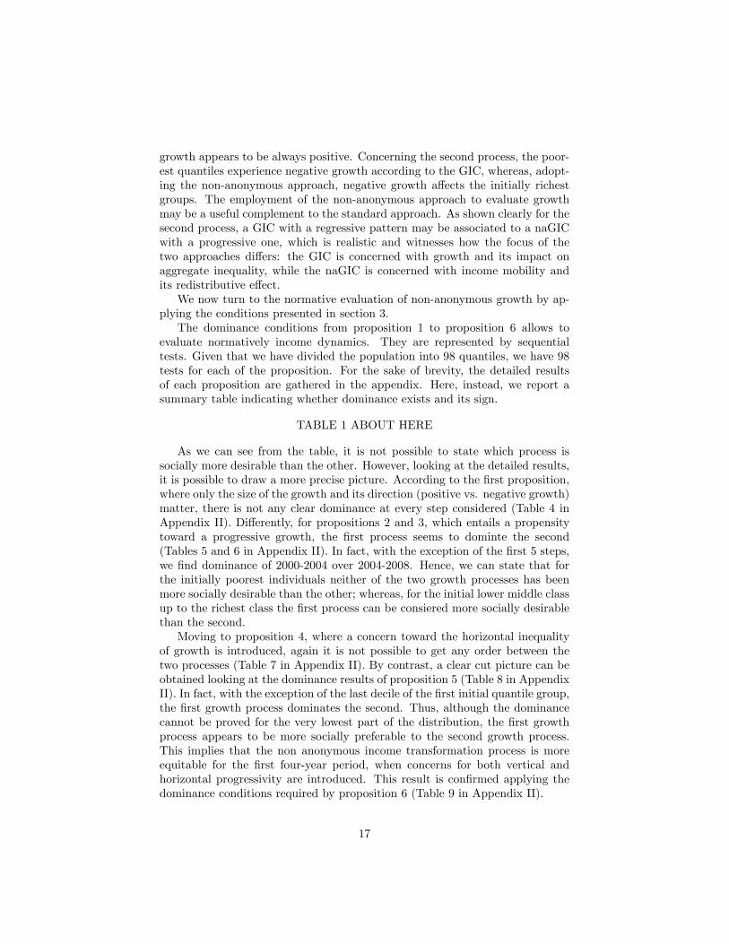
growth appears to be always positive. Concerning the second process, the poor-est quantiles experience negative growth according to the GIC, whereas, adopt-ing the non-anonymous approach, negative growth affects the initially richestgroups. The employment of the non-anonymous approach to evaluate growthmay be a useful complement to the standard approach. As shown clearly for thesecond process, a GIC with a regressive pattern may be associated to a naGICwith a progressive one, which is realistic and witnesses how the focus of thetwo approaches differs: the GIC is concerned with growth and its impact onaggregate inequality, while the naGIC is concerned with income mobility andits redistributive effect.We now turn to the normative evaluation of non-anonymous growth by ap-

plying the conditions presented in section 3.The dominance conditions from proposition 1 to proposition 6 allows to

evaluate normatively income dynamics. They are represented by sequentialtests. Given that we have divided the population into 98 quantiles, we have 98tests for each of the proposition. For the sake of brevity, the detailed resultsof each proposition are gathered in the appendix. Here, instead, we report asummary table indicating whether dominance exists and its sign.

TABLE 1 ABOUT HERE

As we can see from the table, it is not possible to state which process issocially more desirable than the other. However, looking at the detailed results,it is possible to draw a more precise picture. According to the first proposition,where only the size of the growth and its direction (positive vs. negative growth)matter, there is not any clear dominance at every step considered (Table 4 inAppendix II). Differently, for propositions 2 and 3, which entails a propensitytoward a progressive growth, the first process seems to dominte the second(Tables 5 and 6 in Appendix II). In fact, with the exception of the first 5 steps,we find dominance of 2000-2004 over 2004-2008. Hence, we can state that forthe initially poorest individuals neither of the two growth processes has beenmore socially desirable than the other; whereas, for the initial lower middle classup to the richest class the first process can be consiered more socially desirablethan the second.Moving to proposition 4, where a concern toward the horizontal inequality

of growth is introduced, again it is not possible to get any order between thetwo processes (Table 7 in Appendix II). By contrast, a clear cut picture can beobtained looking at the dominance results of proposition 5 (Table 8 in AppendixII). In fact, with the exception of the last decile of the first initial quantile group,the first growth process dominates the second. Thus, although the dominancecannot be proved for the very lowest part of the distribution, the first growthprocess appears to be more socially preferable to the second growth process.This implies that the non anonymous income transformation process is moreequitable for the first four-year period, when concerns for both vertical andhorizontal progressivity are introduced. This result is confirmed applying thedominance conditions required by proposition 6 (Table 9 in Appendix II).

17

The conditions applied till now arise to be very restrictive, since they areaimed at capturing and explaining both aspect of the redistributive effect ofgrowth, that is its vertical and horizontal inequality. Less restrictive conditionsderive when the concern for horizontal equity is relaxed. We thus proceed inour illustration adopting this line of reasoning.We start by applying the dominance condition in proposition 7. They simply

plots the mean of the income change experieced by the individuals ranked thesame in the intial distribution of income against each initial rank. The curvesresulting from proposition 7 are reported in figure 3.

FIGURE 3 ABOUT HERE

We can observe that the two curves are characterized by the same decreasingpattern implying that mobility has been progressive in both period considered,where mobility is meant to capture the variation of individual income in absoluteterm. The poorer the initial quantile group the individuals belong, the higherthe income gain they experience in absolute terms23 .In particular, individuals experiences an increase in income up to the around

the 70th initial quantile. On the contrary, for the initially richest quantilesgroups, growth is almost everywhere negative. Moving to the ordering of the twoprocesses, since the curves intercept continuously, it is not possible to provide acomplete ranking, thus we cannot sate which process is socially better than theother, when what matters is only the size of growth.We now turn to apply the dominance condition of proposition 8, where, in

addition to the size of growth, the vertical equity of growth matters. Theysimply plots the cumulated means of the income change experieced by the indi-viduals ranked the same in the intial distribution of income against each initialrank. The curves resulting from proposition 8 are reported in figure 4.

FIGURE 4 ABOUT HERE

The comparison between the two dynamics is now more clear. The overallabsolute mean income growth - that can be read as the coordinate of the rich-est quantile- are rather different, however the two patterns are similar. Bothcurves increase steeply up to the 80th quantile, take a concave shape in the verylast part of the distribution, thus the curves become decreasing for the richestquantiles. Since we are evaluating levels of income change, this particular shapemeans that income transformation process has been substantially progressive(in absolute term) in the both periods. However, a feature stands out. Thecurve relative to the first process is higher than the second meaning that theextent of growth has been more intensive. By contrast, the concavity appearsto be more pronounced in the second process, implying that this process mighthave been more effective in terms of vertical redistribution. Although thesecurves seems to be very informative in terms of the characteristics of each single

23This confirms the pattern coming out from the naGIC (Fig. 2), which is instead basedon proportionate growth.

18

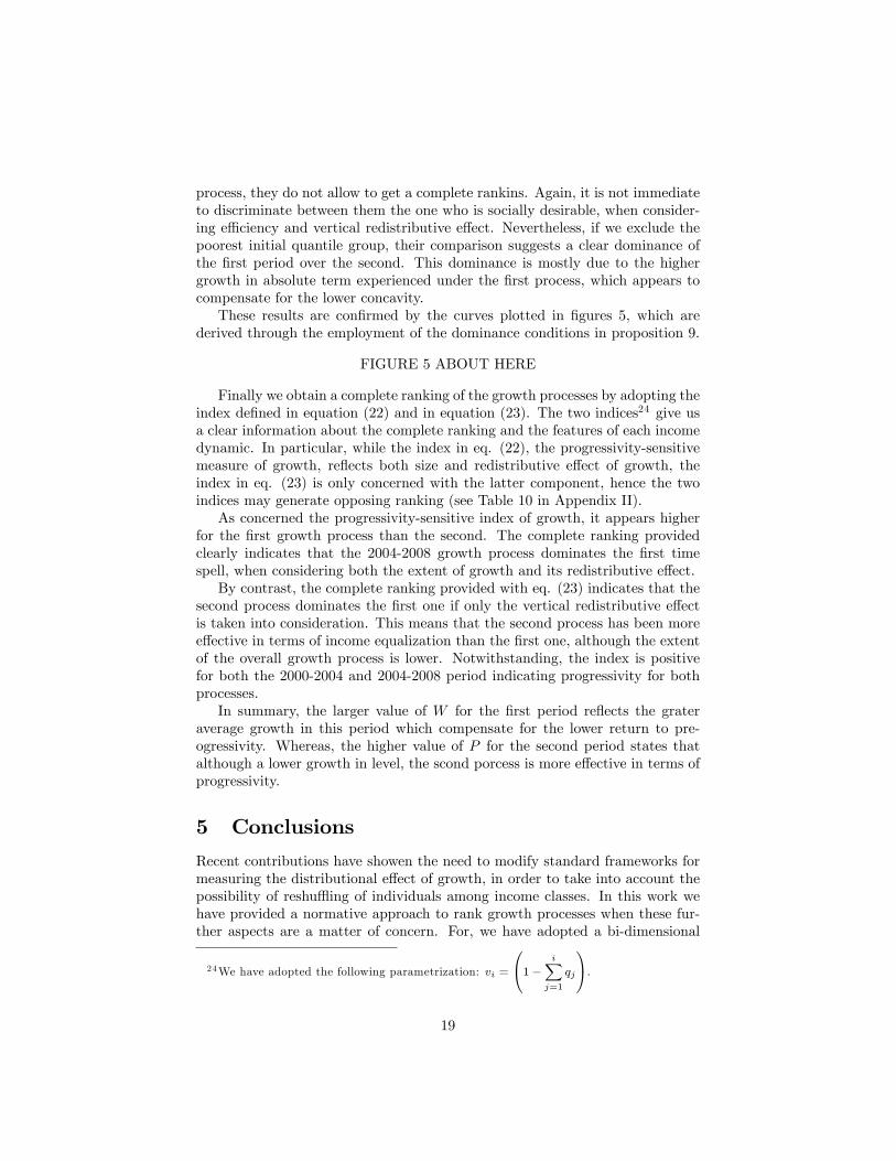
process, they do not allow to get a complete rankins. Again, it is not immediateto discriminate between them the one who is socially desirable, when consider-ing effi ciency and vertical redistributive effect. Nevertheless, if we exclude thepoorest initial quantile group, their comparison suggests a clear dominance ofthe first period over the second. This dominance is mostly due to the highergrowth in absolute term experienced under the first process, which appears tocompensate for the lower concavity.These results are confirmed by the curves plotted in figures 5, which are

derived through the employment of the dominance conditions in proposition 9.

FIGURE 5 ABOUT HERE

Finally we obtain a complete ranking of the growth processes by adopting theindex defined in equation (22) and in equation (23). The two indices24 give usa clear information about the complete ranking and the features of each incomedynamic. In particular, while the index in eq. (22), the progressivity-sensitivemeasure of growth, reflects both size and redistributive effect of growth, theindex in eq. (23) is only concerned with the latter component, hence the twoindices may generate opposing ranking (see Table 10 in Appendix II).As concerned the progressivity-sensitive index of growth, it appears higher

for the first growth process than the second. The complete ranking providedclearly indicates that the 2004-2008 growth process dominates the first timespell, when considering both the extent of growth and its redistributive effect.By contrast, the complete ranking provided with eq. (23) indicates that the

second process dominates the first one if only the vertical redistributive effectis taken into consideration. This means that the second process has been moreeffective in terms of income equalization than the first one, although the extentof the overall growth process is lower. Notwithstanding, the index is positivefor both the 2000-2004 and 2004-2008 period indicating progressivity for bothprocesses.In summary, the larger value of W for the first period reflects the grater

average growth in this period which compensate for the lower return to pre-ogressivity. Whereas, the higher value of P for the second period states thatalthough a lower growth in level, the scond porcess is more effective in terms ofprogressivity.

5 Conclusions

Recent contributions have showen the need to modify standard frameworks formeasuring the distributional effect of growth, in order to take into account thepossibility of reshuffl ing of individuals among income classes. In this work wehave provided a normative approach to rank growth processes when these fur-ther aspects are a matter of concern. For, we have adopted a bi-dimensional

24We have adopted the following parametrization: vi =

1− i∑j=1

qj

.

19

framework, where the two dimensions are respectively the initial rank of indi-viduals and their income transformation. We have proposed to aggregate theseinformation according to a rank dependent approach, which makes it possibleto account for the size of growth and its vertical and horizontal impact. Wehave provided partial dominance conditions for ordering growth processes andwe have shown how these conditions relate to na-GIC. Finally, we have proposedtwo classes of indices: one aimed at capturing at the same time the extent ofgrowth and its vertical redistributive effect; the other aimed at isolating thelatter component. We have then showen how to apply our methodology, usingitalian data, in order to capture the main features of non-anonymous growthprocesse and to order among them.

References

[1] Aaberge, R. (2001): Axiomatic Characterization of the Gini Coeffi cient andLorenz Curve Orderings. Journal of Economic Theory 101, 115-132.

[2] Atkinson, A. B., Bourguignon, F. (1987): Income distribution and dif-ferences in needs. In G. Feiwel (Ed.), Arrow and the Foundations of theTheory of Economic Policy, Macmillan, London, 350-70.

[3] Bénabou, R., Ok, E. (2001): Mobility as progressivity: ranking incomeprocesses according to equality of opportunity, NBER Working Paper No.8431

[4] Bourguignon, F. (2003): The Growth Elasticity of Poverty Reduction: Ex-plaining Heterogeneity across Countries and Time Periods. In: Eicher, T.,Turnovsky, S. Inequality and growth: theory and policy implications. MITPress, Cambridge.

[5] Bourguignon, F. (2004): The Poverty-Growth-Inequality Triangle. IndianCouncil for Research on International Economic Relations, Working PaperN.125.

[6] Bourguignon, F. (2011). Non-anonymous Growth Incidence Curves, IncomeMobility and Social Welfare Dominance, Journal of Economic Inequality,9(4), 605-627DOI: 10.1007/s10888-010-9159-7.

[7] Chambaz, C., Maurin, E. (1998): Atkinson and Bourguignon’s DominanceCriteria: Extended and Applied to the Measurement of Poverty in France.Review of Income and Wealth, 44, 4.

[8] Datt, G., Ravallion, M. (1992): Growth and redistribution components ofchanges in poverty measures: a decomposition with applications to Braziland India in the 1980s. Journal of Development Economics, 38, 275—95

[9] Donaldson, D., Weymark, J. (1980): A Single-Parameter Generalization ofthe Gini Indices of Inequality. Journal of Economic Theory, 22, 67-86

20

[10] Duclos, J. (2009): What is pro-poor?. Social Choice and Welfare, 32, 37-58.

[11] Ebert, U. (1987): Size and Distribution of Incomes as Determinants ofSocial Welfare. Journal of Economic Theory, 41, 23-33.

[12] Essama-Nssah, B. (2005). A Unified Framework for Pro-Poor GrowthAnalysis. Economics Letters, 89, 216-221.

[13] Essama-Nssah, B., Lambert, P. (2009): Measuring Pro-poorness: a Uni-fying Approach with New Results. Review of Income and Wealth, 55, 3,752-778.

[14] Ferreira, F. H. G. (2010): Distributions in motion. Economic growth, in-equality, and poverty dynamics. World Bank, Policy research working paperworking paper N. 5424.

[15] Gottschalck, P., Moffi tt, R. (2009). The rising instability of U.S. earnings,Journal of Economic Perspectives, 23(4), 3-24.

[16] Grimm, M. (2007): Removing the anonymity axiom in assessing pro-poorgrowth. Journal of Economic Inequality, 5(2), 179-197.

[17] Grosse, M., Harttgen, K., Klasen, S. (2008): Measuring Pro-poor Growthin Non-income Dimensions. World Development, 36, 6, 1021-1047.

[18] Jenkins, S., Lambert, P. (1993): Ranking income distributions when needsdiffer. Review of Income and Wealth, 39, 4.

[19] Jenkins, S., Van Kerm, P. (2004): Accounting for Income DistributionTrends: A Density Function Decomposition Approach. IZA Discussion Pa-per No. 1141.

[20] Jenkins, S., Van Kern, P. (2006): Trends in income inequality, pro-poorincome growth and income mobility, Oxford Economic Papers, 58, 3, 531-48.

[21] Jenkins, S., Van Kerm, P. (2011): Trends in individual income growth:measurement methods and British evidence. IZA DP. No. 5510.

[22] Kakwani, N., Pernia, E. (2000): What is Pro-poor Growth?. Asian Devel-opment Review, 18, 1-16.

[23] Kakwani, N., Son, H. (2008): Poverty Equivalent Growth Rate. Review ofIncome and Wealth, 54, 4, 643-655.

[24] Klasen, S., Misselhorn, M. (2008): Determinants of the Growth Semi-elasticity of Poverty Reduction. EUDN, Working Paper N. 2008-11.

[25] Kraay, A. (2006): When is Growth Pro-poor? Evidence From a Panel ofCountries. Journal of Development Economics, 80, 1, 198-227.

21

[26] Peragine, V. (2002): Opportunity Egalitarianism and Income Inequality:the rank dependent approach. Mathematical Social Sciences, 44, 45-64.

[27] Ravallion, M., Chen, S. (2003): Measuring pro-poor growth. EconomicsLetters, 78, 1, 93—9.

[28] Son, H. H. (2004): A note on pro-poor growth. Economics Letters 82, 3,307—314.

[29] Van Kerm, P. (2006): Comparisons of income mobility profiles. IRISSWorking Paper 2006/03, CEPS/INSTEAD, Differdange, Luxembourg.

[30] Van Kerm, P. (2009): Income mobility profiles. Economic Letters, 102, 2,93-95.

[31] Weymark, J. (1981): Generalised Gini Inequality Indices. MathematicalSocial Sciences, 1, 409-430.

[32] Yaari, M. (1988): A Controversial Proposal Concerning Inequality Mea-surement. Journal of Economic Theory, 44, 381-397.

[33] Zheng, B. (2010): Consistent Comparison of Pro-poor Growth, SocialChoice and Welfare, July 2010.

[34] Zoli, C. (2000): Inverse Sequential Stochastic Dominance: Rank-DependentWelfare, Deprivation and Poverty Measurement. Discussion Paper in Eco-nomics, No. 00/11, University of Nottingham.

Appendix I

Proof of Proposition 1We want to find a necessary and suffi cient condition for

∆W (F (x | y)) =

n∑i=1

1∫0

vi (p) [xAi (p)− xBi (p)] dp ≥ 0, ∀W ∈W1 (25)

Suffi ciency clearly derives from the fact that since vi (p) ≥ 0, ∀p ∈ [0, 1] and∀i = 1, 2, ...,m, xAi (p) − xAi (p) ≥ 0, ∀p ∈ [0, 1] and ∀i = 1, 2, ..., n, implies∆W (F (x | y)) ≥ 0.For the necessity, suppose for a contradiction that∆W (F (x | y)) ≥ 0, ∀W ∈

W1, but there is a quantile group h ∈ {1, ..., n} and an interval I ≡ [a, b] ⊆[0, 1] such that xAh (p) − xBh (p) < 0,∀p ∈ I. Now select a set of function{vi (p)}i∈{1,...,m} such that vi (p)↘ 0, ∀i 6= h and vh (p)↘ 0, ∀p ∈ [0, 1] \ I. in

this case ∆W (F (x | y)) would reduce to

b∫a

vh (p) [xAh (p)− xBh (p)] dp < 0, a

contradiction. QED

22

Proof of Proposition 2Before proving this proposition we need to prove the following lemma.

Lemma 1n∑k=1

vkwk ≥ 0 for all sets of numbers {vk} such that vk ≥ vk+1 ≥ 0

∀k ∈ {1, ..., n} if and only ifk∑i=1

wi ≥ 0, ∀k ∈ {1, ..., n}.

Proof. Applying Abel’s decomposition:n∑k=1

vkwk =

n∑k=1

(vk − vk+1)k∑i=1

wi. If

k∑i=1

wi ≥ 0, ∀k ∈ {1, ..., n}, thenn∑k=1

vkwk ≥ 0. As for the necessity part,

suppose thatn∑k=1

vkwk ≥ 0 for all sets of numbers {vk} such that vk ≥ vk+1 ≥ 0,

but ∃j ∈ {1, ..., n} :

j∑i=1

wi < 0. Consider what happens when (vk − vk+1) ↘

0,∀k 6= j. We obtain thatn∑k=1

vkwk −→ (vj − vj+1)j∑i=1

wi < 0, a contradiction.

We now want to find a necessary and suffi cient condition for

∆W (F (x | y)) =

n∑i=1

1∫0

vi (p) [xAi (p)− xBi (p)] dp ≥ 0, ∀W ∈W12 (26)

Suffi ciency can be shown as follows. First, reverse the order of integration andsummation, such that

∆W (F (x | y)) =

1∫0

n∑i=1

vi (p) [xAi (p)− xBi (p)] dp ≥ 0 (27)

Letting Si (p) = xAi (p)− xBi (p) and rewriting (27):

∆W (F (x | y)) =

1∫0

n∑i=1

vi (p)Si (p) dp ≥ 0 (28)

Since vi (p) ≥ vi+1 (p) ≥ 0, ∀i = 1, ..., n−1 and ∀p ∈ [0, 1], we can apply Lemma

1 and obtain thatn∑i=1

vi (p)Si (p) ≥ 0 if and only ifk∑i=1

Si (p) ≥ 0,∀k = 1, ..., n

23

and ∀p ∈ [0, 1]. It follows thatn∑i=1

vi (p)Si (p) ≥ 0, ∀p ∈ [0, 1], implies that,

integrating with respect to p,

1∫0

n∑i=1

vi (p)Si (p) dp ≥ 0.

For the necessity, suppose for a contradiction that∆W (F (x | y)) ≥ 0, ∀W ∈W12, but there is an initial quantile h ∈ {1, ..., n} and an interval I ≡ [a, b] ⊆

[0, 1] such thath∑i=1

Si (p) < 0,∀p ∈ I. Now, applying Lemma 1, there exists a set

of functions {vi (p) ≥ 0} : [0, 1] −→ <+, i = 1, ..., n, such thatn∑i=1

vi (p)Si (p) <

0, ∀p ∈ I. Writingn∑i=1

vi (p)Si (p) = T (p),∆W (F (x | y)) reduces to

1∫0

T (p) dp,

where T (p) < 0, ∀p ∈ I. Selecting a set of function T (p), such that T (p) −→ 0,

∀p ∈ [0, 1] \ I, ∆W (F (x | y)) would reduce to

b∫a

T (p) dp < 0, a contradiction.

QED

Proof of Proposition 3We want to find a necessary and suffi cient condition for

∆W (F (x | y)) =

n∑i=1

1∫0

vi (p) [xAi (p)− xBi (p)] dp ≥ 0, ∀W ∈W123 (29)

For the suffi ciency, note that if vi (p) satisfies axiom 1, 2, and 3, we canrevert the order of integration and summation and apply Abel’s decomposi-

tion to obtain: ∆W (F (x | y)) =

1∫0

[n∑i=1

(vi (p)− vi+1 (p))

i∑k=1

Sk (p)

]dp, where

Sk (p) = xAk (p)−xBk (p). Let vi (p)− vi+1 (p) = ωi (p) andi∑

k=1

Sk (p) = κi (p),

by axiom 3 ωi (p) > ωi+1 (p), ∀i = 1, ..., n − 1, ∀p ∈ [0, 1]. We can apply

Lemma 1 to getm∑i=1

ωi (p)κi (p) ≥ 0 if and only ifj∑i=1

κi (p) ≥ 0, ∀j = 1, ..., n,

∀p ∈ [0, 1]. Ifn∑i=1

ωi (p)κi (p) ≥ 0, ∀p ∈ [0, 1], implies that ∆W (F (x | y)) =

1∫0

n∑i=1

ωi (p)κi (p) dp ≥ 0. Thusj∑i=1

i∑k=1

xAi (p)−xBi (p), ∀j = 1, ..., n, ∀p ∈ [0, 1]

is suffi cient for ∆W (F (x | y)) ≥ 0.

24

For the necessity, let T (p) ≡n∑i=1

ωi (p)κi (p), we can write the following

∆W (F (x | y)) =

1∫0

T (p) dp. Suppose that ∆W (F (x | y)) ≥ 0, ∀W ∈ W123,

but ∃h = 1, ...,m and ∃I ≡ [a, b] ⊆ [0, 1] such thath∑i=1

κi (p) < 0, ∀p ∈ I. Then

by Lemma 1 ∃ a set of functions ωi (p) : [0, 1] −→ <+, i = 1, ..., n, such thatT (p) < 0, ∀p ∈ I. We can chose a function T (p) such that T (p) −→ 0, ∀p ∈

[0, 1]�I, thus ∆W (F (x | y)) would reduce to

b∫a

T (p) dp < 0, a contradiction.

QED

Proof of Proposition 4We want to find a necessary and suffi cient condition for

∆W (F (x | y)) =

n∑i=1

1∫0

vi (p) [xAi (p)− xBi (p)] dp ≥ 0, ∀W ∈W14 (30)

For the suffi ciency, let Si (p) = xAi (p) − xBi (p), we can integrate eq. (30)by parts to get:

∆W (F (x | y)) =

n∑i=1

vi (1)

1∫0

Si (p) dp

− n∑i=1

1∫0

v′i (p)

p∫0

Si (t) dtdp (31)

It follows that

p∫0

xAi (t)− xBi (t) dt ≥ 0,∀p ∈ [0, 1] ,∀i = 1, ..., n (32)

is suffi cient for welfare dominance, since by axiom 1 vi (p) ≥ 0 eq. (31) im-

plies the positivity of vi (1)

1∫0

Si (p) dp and by axiom 4 v′i (p) ≤ 0 it implies the

negativity of the second term of eq. (31). It follows that ∆W (F (x | y)) ≥ 0.For the necessity, suppose that ∆W (F (x | y)) ≥ 0, but ∃h = 1, ...,m and

∃I ≡ [a, b] ⊆ [0, 1] such that

p∫0

xAh (t) − xBh (t) dt < 0, ∀p ∈ I. Let Ti (p) =

v′i (p)

p∫0

xAi (t) − xBi (t) dt, ∀i = 1, ..., n, ∀p ∈ [0, 1]. We can chose a set of

25

functions Ti (p) such that Ti (p) −→ 0, ∀i 6= h and T (p) −→ 0, ∀p ∈ [0, 1]�I.Given the negativity of v′i (p), Th (p) < 0, ∀p ∈ I. Then ∆W (F (x | y)) =

n∑i=1

vi (1)

1∫0

Si (p) dp−b∫a

Th (p) dp. It is always possible to chose a combination

of vi (1) and Si (p) such thatn∑i=1

vi (1)

1∫0

Si (p) dp ≤ 0. Then, ∆W (F (x | y)) =

−b∫a

Th (p) dp ≤ 0, a contradiction. QED

Proof of Proposition 5We want to find a necessary and suffi cient condition for

∆W (F (x | y)) =

n∑i=1

1∫0

vi (p) [xAi (p)− xBi (p)] dp ≥ 0, ∀W ∈W1245 (33)

Suffi ciency can be shown as follows. First, reverse the order of integrationand summation, such that

∆W (F (x | y)) =

1∫0

n∑i=1

vi (p) [xAi (p)− xBi (p)] dp ≥ 0 (34)

Letting Si (p) = xAi (p) − xBi (p) and εi (p) = vi (p) − vi+1 (p) ≥ 0, ∀i =1, ...,m− 1 and ∀p ∈ [0, 1], by axiom 1 and application of Abel’s decompositionwe can rewrite eq. (34):

∆W (F (x | y)) =

1∫0

n∑i=1

εi (p)

i∑j=1

Sj (p)

dp ≥ 0 (35)

Integrating by parts

∆W (F (x | y)) =

n∑i=1

εi (1)

i∑j=1

1∫0

Sj (p) dp

− (36)

1∫0

n∑i=1

ε′i (p)

i∑j=1

p∫0

Sj (t) dt

dp ≥ 0

By axiom 2 εi (1) ≥ 0, by axiom 4 and 5 ε′

i (p) ≤ 0, ∀i = 1, ..., n and ∀p ∈

[0, 1], it follows thati∑

j=1

p∫0

Sj (t) dt ≥ 0,∀i = 1, ..., n and ∀p ∈ [0, 1] implies

∆W (F (x | y)) ≥ 0.

26

For the necessity, suppose for a contradiction that ∆W (F (x | y)) ≥ 0, butthere is an initial quantile h ∈ {1, ..., n} and an interval I ≡ [a, b] ⊆ [0, 1] such

thath∑j=1

p∫0

Sj (t) dt < 0,∀p ∈ I. Now, applying Lemma 1 in Chambaz and

Maurin (1998), there exists a set of non-positive functions{ε′

i (p) ≤ 0}i∈{1,...,n}

such thatn∑i=1

ε′

i (p)

i∑j=1

p∫0

Sj (t) dt

> 0, ∀p ∈ I.

Now let R (p) =

n∑i=1

ε′

i (p)

i∑i=1

p∫0

Si (t) dt

, then R (p) ≥ 0, ∀p ∈ I. Then,

∆W (F (x | y)) =

n∑i=1

εi (1)

i∑j=1

1∫0

Sj (p) dp

− 1∫0

R (p) dp.

Now choosing R (p) such that R (p) −→ 0 for some p ∈ [0, 1] \ I,

∆W (F (x | y)) =

n∑i=1

εi (1)

i∑j=1

1∫0

Sj (p) dp

− b∫a

R (p) dp

We can choose εi (1) = 0, ∀i = 1, ..., n, or we can choose a combination

of εi (1) andi∑

j=1

1∫0

Sj (p) dp, such thatn∑i=1

εi (1)

i∑j=1

1∫0

Sj (p) dp

= 0, then

∆W (F (x | y)) = −b∫a

R (p) dp ≤ 0, a desired contradiction. QED.

Proof of proposition 6We want to find necessary and suffi cient conditions for

∆W =

n∑i=1

1∫0

vi (p)xAi (p) dp−n∑i=1

1∫0

vi (p)xBi (p) dp ≥ 0 (37)

where v′i−1 (p)− v′i (p) < v′i (p)− v′i+1 (p) < 0.For the suffi ciency, let Si (p) = ∆W = xAi (p)− xBi (p)

∆W =

n∑i=1

1∫0

vi (p)Si (p) dp ≥ 0 (38)

Integrating by parts

27

∆W =

n∑i=1

vi (1)

1∫0

Si (p) dp−n∑i=1

1∫0

v′i (p)

p∫0

Si (t) dt ≥ 0 (39)

Simplifying

∆W =

n∑i=1

vi (1) (µFi − µGi)−n∑i=1

1∫0

v′i (p)

p∫0

Si (t) dt = (40)

=

n∑i=1

vi (1) (µFi − µGi)−1∫0

n∑i=1

v′i (p)

p∫0

Si (t) dt ≥ 0 (41)

By axiom 4 and 5 v′i (p)− v′i+1 (p) = w′i (p) ≤ 0.For analytical convenience let w′i (p) = −zi (p), where zi (p) > 0, such that

w′i+1 (p) = −zi+1 (p), by axiom 6 zi (p) > zi+1 (p)

∆W =

n∑i=1

vi (1) (µFi − µGi) +

1∫0

n∑i=1

zi (p)

i∑k=1

p∫0

Sk (t) dt = (42)

=

n∑i=1

vi (1) (µFi − µGi) +

1∫0

n∑i=1

zi (p)− zi+1 (p)

i∑k=1

k∑j=1

p∫0

Sk (t) dt ≥ 0 (43)

By axiom 1 and 2 vi (p)− vi+1 (p) > 0

∆W =

n∑i=1

vi (1)−vi+1 (1)

i∑k=1

(µFk − µGk)+

1∫0

n∑i=1

zi (p)−zi+1 (p)

i∑k=1

k∑j=1

p∫0

Sj (t) dt ≥ 0

(44)

Let vi (p)− vi−1 (p) = wi−1 (p)

∆W =

n∑i=1

wi (1)

i∑k=1

(µFk − µGk)+

1∫0

n∑i=1

zi (p)−zi+1 (p)

i∑k=1

k∑j=1

p∫0

Sj (t) dt ≥ 0

(45)Also, by axiom 3 wi (p) > wi+1 (p) > 0

∆W =

n∑i=1

wi (1)−wi+1 (1)

i∑k=1

k∑j=1

(µFj − µGj

)+

1∫0

n∑i=1

zi (p)−zi+1 (p)

i∑k=1

k∑j=1

p∫0

Sj (t) dt ≥ 0

(46)

28

It follows that

i∑k=1

k∑j=1

p∫0

Sj (t) dt ≥ 0,∀i = 1, ..., n, ∀p ∈ [0, 1] (47)

is suffi cient for∆W ≥ 0. In fact, if eq. (47) holds, theni∑

k=1

k∑j=1

(µFj − µGj

)≥

0, ∀i = 1, ..., n,

And ifi∑

k=1

k∑j=1

p∫0

Sj (t) dt ≥ 0, ∀i = 1, ..., n, also holds ∀p ∈ [0, 1],

then it must be the case that

1∫0

n∑i=1

zi (p)− zi+1 (p)

i∑k=1

k∑j=1

p∫0

Sj (t) dt ≥ 0.

For the necessity: suppose that ∆W ≥ 0, but ∃h = 1, ...,m and ∃I ∈ [a, b] ⊆[0, 1]

such thath∑k=1

k∑j=1

p∫0

Sj (t) dt ≤ 0, ∀p ∈ I.

By lemma 1, this implies that there is a function zi (p)

such thatn∑i=1

zi (p)− zi+1 (p)

i∑k=1

k∑j=1

p∫0

Sj (t) dt ≤ 0, ∀p ∈ I.

Let T (p) ≡n∑i=1

zi (p)−zi+1 (p)

i∑k=1

k∑j=1

p∫0

Sj (t) dt, ∀p ∈ [0, 1];

b∫a

T (p) dp < 0.

We can chose a function T (p) −→ 0, ∀p ∈ [0, 1]�I.

This implies that ∆W =

n∑i=1

wi (1)

i∑k=1

(µFi − µGi) +

b∫a

T (p) dp. It is always

possible to chose a combination of wi (1) and µFi−µGi such thatn∑i=1

wi (1)

i∑k=1

(µFi − µGi) =

0. It follows that ∆W =

b∫a

T (p) dp ≤ 0 a contradiction. QED

Proof of Proposition 7We want to find a necessary and suffi cient condition for

∆W (F (x | y)) =

n∑i=1

1∫0

vi (p) [xAi (p)− xBi (p)] dp ≥ 0, ∀W ∈W17 (48)

For the suffi ciency, by axiom 7 vi (p) = βi, ∀p ∈ [0, 1] and ∀i = 1, 2, ..., n,therefore we can write eq. (48) as follows:

29

∆W (F (x | y)) =

n∑i=1

βi

1∫0

[xAi (p)− xBi (p)] dp =

=

n∑i=1

βi [µAi − µBi] ≥ 0 (49)

by axiom 1 vi (p) = βi ≥ 0, ∀p ∈ [0, 1] and ∀i = 1, 2, ..., n, ∆W (F (x | y)) ≥ 0 ifµAi − µBi ≥ 0, ∀i = 1, ..., n.For the necessity, suppose that

∆W (F (x | y)) =

n∑i=1

βi [µAi − µBi] ≥ 0

but ∃k = 1, ..., n such that µAk < µBk. We can choose a set of numbers{βi}i=1,...,n such that βi ↘ 0, ∀i 6= k. ∆W (F (x | y)) would reduce to βk (µAk − µBk) <0, a contradiction. QED

Proof of Proposition 8We want to find a necessary and suffi cient condition for

∆W (F (x | y)) =

n∑i=1

1∫0

vi (p) [xAi (p)− xBi (p)] dp ≥ 0, ∀W ∈W127 (50)

For both conditions, note that by axiom 7 we can write: ∆W (F (x | y))

=

n∑i=1

βi [µAi − µBi] ≥ 0. Let Si = [µAi − µBi], ∀i = 1, ..., n. Since by axiom

2 βi ≥ βi+1 and βi ≥ 0 by axiom 1, we can apply Lemma 1. Therefore,

∆W (F (x | y)) =

n∑i=1

βiSi ≥ 0 if and only ifk∑i=1

Si ≥ 0, ∀k = 1, ..., n. Hence,

∆W (F (x | y)) ≥ 0 if and only ifk∑i=1

µAi − µBi, ∀k = 1, ..., n. QED

Proof of Proposition 9We want to find a necessary and suffi cient condition for

∆W (F (x | y)) =

n∑i=1

1∫0

vi (p) [xAi (p)− xBi (p)] dp ≥ 0, ∀W ∈W1237 (51)

For both conditions note that we can apply axiom 1, 2, 3 and 7 and Abel’s

decomposition as follows: ∆W =

n∑i=1

(βi − βi+1

) i∑k=1

Sk, where Sk = µAk−µBk.

30

Leti∑

k=1

Sk = κk and βi − βi+1 = ωi, by axiom 3 ωi > ωi+1, ∀i = 1, ..., n − 1.

Applying Lemma 1, ∆W (F (x | y)) =

n∑i=1

ωiκi ≥ 0 if and only ifj∑i=1

i∑k=1

κk ≥ 0,

∀j = 1, ..., n. Substituting in the above expression: ∆W (F (x | y)) ≥ 0 if and

only ifj∑i=1

i∑k=1

µAk ≥j∑i=1

i∑k=1

µBk, ∀j = 1, ..., n. QED

31

Figures and tables (Text)

Figure 1: GICs 2000-2004 vs. 2004-2008. Surces: Authors’calculation from SHIW.

Figure 2: naGICs 2000-2004 vs. 2004-2008. Surces: Authors’calculation from SHIW.

-10

010

2030

40%

inco

me

grow

th

0 20 40 60 80 100initial rank

GIC 2000-2004 GIC 2004-2008

Italian GICs 2000-2004 vs. 2004-2008

-.5

0.5

11.

5%

inco

me

grow

th

0 20 40 60 80 100initial rank

naGIC 2000-2004 naGIC 2004-2008

Italian naGICs 2000-2004 vs. 2004-2008

Table 1: 2002-2004 VS 2004-2008. Results of the dominance conditions from proposition 1 to proposition 6. Surces: Authors’calculation from SHIW.

Sing of the dominance 2000-2004 VS 2004-2008

Prop. 1 Prop. 2 Prop. 3 Prop. 4 Prop. 5 Prop. 6

+

-

Nc X X X X X X

Figure 3: Curves Proposition 7. 2000-2004 VS 2004-2008. Surces: Authors’calculation from SHIW.

-10

000

-50

000

5000

leve

ls o

f inc

ome

grow

th

0 20 40 60 80 100initial rank

income change 2000-2004 income change 2004-2008

Italian growth: 2000-2004 vs. 2004-2008

Figure 4: Curves Proposition 8. 2000-2004 VS 2004-2008. Surces: Authors’calculation from SHIW.

Figure 5: Curves Proposition 9. 2000-2004 VS 2004-2008. Surces: Authors’calculation from SHIW.

050

000

1000

0015

0000

leve

ls o

f in

com

e gr

owth

0 20 40 60 80 100initial rank

Income change 2000-2004 Income change 2004-2008

Italian growth: 2000-2004 vs 2004-20080

2000

0004

0000

006

000

0008

0000

001.

00e+

07le

vels

of i

ncom

e gr

owth

0 20 40 60 80 100initial rank

Income change 2000-2004 Income change 2004-2008

Italian growth: 2000-2004 vs. 2004-2008

Figures and tables (Appendix II) Table 2: 2002-2004 VS 2004-2008. Percentage income growth at each quantile. Surces: Authors’calculation from SHIW.

Initial

rank GIC 2000-2004 GIC 2004-2008

1 -8,79 41,13

2 2,63 15,89

3 -1,60 19,83

4 1,35 14,87

5 4,67 13,85

6 5,10 13,20

7 7,62 99,68

8 7,34 14,43

9 9,60 12,87

10 11,49 15,16

11 10,03 10,16

12 10,26 9,97

13 9,19 11,45

14 10,22 10,48

15 11,63 11,47

16 12,89 9,79

17 14,52 11,85

18 14,55 12,25

19 15,59 14,50

20 14,95 13,00

21 14,46 12,07

22 13,41 12,89

23 11,32 13,08

24 13,01 12,46

25 11,64 12,40

26 12,38 11,71

27 11,96 12,51

28 11,33 12,32

29 11,48 13,30

30 13,04 12,75

31 11,30 13,19

32 12,42 13,01

33 12,03 12,78

34 11,91 12,39

35 11,54 13,20

36 11,72 12,06

37 11,87 14,07

38 12,41 14,70

39 11,27 15,53

40 11,25 14,44

41 10,41 14,37

42 9,92 14,93

43 9,63 13,92

44 9,51 13,72

45 9,52 13,11

46 8,82 14,01

47 8,80 13,35

48 7,31 12,33

49 6,64 12,45

50 7,02 12,44

51 6,90 12,30

52 6,42 13,31

53 6,90 12,71

54 7,07 12,28

55 7,02 13,15

56 7,15 13,03

57 7,27 12,03

58 6,81 12,51

59 8,06 11,83

60 8,25 11,42

61 7,51 11,79

62 7,34 12,59

63 8,37 12,49

64 8,82 12,99

65 10,11 13,43

66 10,50 14,49

67 96,13 14,79

68 10,55 14,58

69 10,12 14,48

70 9,04 13,90

71 8,33 13,18

72 8,01 13,10

73 8,21 13,03

74 7,73 12,48

75 7,66 12,45

76 8,22 12,87

77 8,71 11,47

78 8,88 9,96

79 8,46 9,83

80 7,87 8,91

81 8,22 10,40

82 8,67 10,71

83 8,43 11,09

84 8,98 11,67

85 8,52 13,10

86 9,08 13,67

87 10,70 13,70

88 9,96 14,92

89 10,48 14,39

90 9,39 13,72

91 8,72 14,60

92 10,71 13,75

93 11,11 15,83

94 9,31 16,49

95 5,92 13,50

96 8,69 11,65

97 6,36 12,58

98 4,35 13,83

Table 3: 2002-2004 VS 2004-2008. Percentage income growth at each initial quantile. Surces: Authors’calculation from SHIW.

Initial

rank

naGIC

2000-2004

naGIC

2004-2008

1 170,94 152,93

2 131,13 87,93

3 117,25 94,26

4 65,59 79,55

5 93,44 47,71

6 78,08 57,19

7 63,58 37,23

8 63,45 70,63

9 62,06 40,55

10 47,41 55,39

11 67,20 32,82

12 22,77 94,68

13 31,90 26,65

14 36,70 25,43

15 77,44 49,22

16 30,52 31,14

17 68,37 17,04

18 50,36 36,69

19 83,89 39,79

20 15,68 27,02

21 37,96 27,46

22 31,03 26,31

23 53,04 24,71

24 27,79 36,23

25 48,77 10,18

26 25,29 42,25

27 40,65 14,29

28 19,06 21,91

29 48,98 34,41

30 20,34 41,35

31 33,40 16,67

32 27,47 13,73

33 10,60 21,07

34 25,09 16,52

35 18,66 13,71

36 11,06 26,44

37 29,46 20,43

38 29,32 18,76

39 21,13 17,92

40 22,19 1,54

41 17,16 27,05

42 13,16 23,06

43 7,45 21,02

44 26,99 13,57

45 12,13 19,24

46 10,79 4,22

47 20,23 10,86

48 19,28 10,95

49 23,75 9,40

50 5,44 30,04

51 43,68 5,24

52 20,05 7,82

53 6,37 8,63

54 4,18 10,59

55 14,22 17,25

56 2,92 16,53

57 20,10 5,21

58 7,25 3,34

59 11,58 29,31

60 20,26 5,46

61 6,21 5,25

62 12,39 2,72

63 8,41 17,85

64 4,06 18,78

65 14,75 11,15

66 2,54 17,45

67 17,88 4,60

68 18,40 7,62

69 -3,33 -2,68

70 -4,59 5,59

71 12,44 -3,64

72 3,29 -8,98

73 -0,11 4,08

74 8,94 4,11

75 5,56 10,28

76 6,64 6,78

77 2,64 8,70

78 7,58 9,70

79 8,38 4,82

80 2,01 -1,00

81 5,37 -1,68

82 0,71 -2,13

83 -2,47 -6,08

84 4,60 -12,44

85 -8,00 -9,85

86 -6,53 -7,85

87 -9,82 -10,68

88 4,12 1,75

89 -2,00 -0,72

90 2,80 -10,21

91 -4,03 -7,07

92 -5,88 -10,32

93 -10,91 -1,10

94 -5,98 -13,26

95 -18,48 -18,42

96 -14,37 -13,52

97 -18,52 -18,12

98 -26,77 -23,22

Table 4: 2002-2004 VS 2004-2008. Results of the dominance conditions from proposition 1. Surces: Authors’calculation from SHIW.

Initial rank Deciles of income change of each initial group

1 2 3 4 5 6 7 8 9 10

1 + + + + + + + + - -

2 - - + + + + + + + +

3 - - - - - + + + + +

4 + + - - - - - + + -

5 + + + + + + + + + +

6 + + + + + - - - + +

7 - - - - - + + + + +

8 - - - - - - + + + +

9 + + + + - + + - + +

10 + + + + + - - - - -

11 - - - + + + + + + +

12 - - - - - - - + - -

13 + + + + + + + + - -

14 + + + + + + + + + -

15 + + + - + + + + + -

16 + - - - - - - - - +

17 - - + + + + + + + +

18 + - - + + - + + - +

19 + + + + + + + + + +

20 - - - - - + - - - -

21 - - - + + + + + + +

22 + + + + - - - + + +

23 + + + + + + + + + +

24 + + + + - - - - - -

25 + + + + + + + + + +

26 - - - - + - - - - -

27 + - + + + + + + + +

28 + - - - - - - - - +

29 + + - - + + + + + +

30 + - - - - + - - - -

31 + + - + + + - - + +

32 - + + + + + + + + +

33 + - - - - - - - - -

34 + + + + + + + - + -

35 - + + + + + + + + -

36 - + + + - - - - - -

37 - - - - - + + + + +

38 - - - + + + - + + +

39 + + - + - - - + + -

40 + - + + + + + + + +

41 - - - - - - - - - -

42 - + - - - - - - - -

43 + - - - - - - - - -

44 - - + + + + + + + +

45 - + - + + + - - + -

46 + + + - + + + + + +

47 + + + + - + + + + +

48 - - - + + + + + + +

49 - + + + + + + + + +

50 - - - - - - - - - -

51 + + + + + + + + + +

52 + + + + + - + + + +

53 + - + + - - - - - -

54 - - - - + + + - - -

55 - - - + + + - - - -

56 - - - - + + - - - -

57 + + + + + + + + + +

58 + + + + + - - - - +

59 + - - - - - - - - -

60 - + + + + + + + + +

61 + - - - - - - - + +

62 + + - + - + + + + +

63 + - - - - - - - - +

64 + - - - - - - - - -

65 + + + - + - - + + -

66 + + + - - - + + + -

67 + + + + + + + + + +

68 + + + + + + + - - +

69 + - - - - - - + + +

70 - - - - - - + - - +

71 + + + + + + + + + +

72 - + + + + + + + + +

73 + + - - - - - - + -

74 + + - - - + + - + +

75 + + - - - - - - + -

76 + + + + + + - - - -

77 - - - - - - - - + -

78 + - - - - + + + + -

79 + - - - - - - + + +

80 + + - + - - + - - +

81 + + + + + + + - - -

82 - + + + - - - - + +

83 - + + + - + - - + +

84 + + + + + + + + + +

85 + + - - - - - - - +

86 + + + + - - - - - -

87 - - + + + + + + + -

88 + + + + + - - - - -

89 + - + + - - - - + -

90 + + + + + + + + + +

91 + + - + - + - - + -

92 - + + + + + + + + +

93 + - - - - - - - - -

94 + + + + + + + + + -

95 + - - + - - - + + -

96 - + + - - + + - - +

97 + + + + - + + - + -

98 - - + - + - + - - -

+ : The process 2000-2004 dominates the process 2004-2008 - : The process 2000-2004 does not dominate the process 2004-2008 Table 5: 2000-2004 VS 2004-2008. Results of the dominance conditions from proposition 2. Surces:

Authors’calculation from SHIW.

Initial rank Deciles of income change of each initial group

1 2 3 4 5 6 7 8 9 10

1 + + + + + + + + - -

2 + + + + + + + + - -

3 + + + + + + + + - -

4 + + + + + + + + - -

5 + + + + + + + + + +

6 + + + + + + + + + +

7 + + + + + + + + + +

8 + + + - + + + + + +

9 + + + + + + + + + +

10 + + + + + + + + + +

11 + + + + + + + + + +

12 + + + + - + + + + +

13 + + + + + + + + + +

14 + + + + + + + + + +

15 + + + + + + + + + +

16 + + + + + + + + + +

17 + + + + + + + + + +

18 + + + + + + + + + +

19 + + + + + + + + + +

20 + + + + + + + + + +

21 + + + + + + + + + +

22 + + + + + + + + + +

23 + + + + + + + + + +

24 + + + + + + + + + +

25 + + + + + + + + + +

26 + + + + + + + + + +

27 + + + + + + + + + +

28 + + + + + + + + + +

29 + + + + + + + + + +

30 + + + + + + + + + +

31 + + + + + + + + + +

32 + + + + + + + + + +

33 + + + + + + + + + +

34 + + + + + + + + + +

35 + + + + + + + + + +

36 + + + + + + + + + +

37 + + + + + + + + + +

38 + + + + + + + + + +

39 + + + + + + + + + +

40 + + + + + + + + + +

41 + + + + + + + + + +

42 + + + + + + + + + +

43 + + + + + + + + + +

44 + + + + + + + + + +

45 + + + + + + + + + +

46 + + + + + + + + + +

47 + + + + + + + + + +

48 + + + + + + + + + +

49 + + + + + + + + + +

50 + + + + + + + + + +

51 + + + + + + + + + +

52 + + + + + + + + + +

53 + + + + + + + + + +

54 + + + + + + + + + +

55 + + + + + + + + + +

56 + + + + + + + + + +

57 + + + + + + + + + +

58 + + + + + + + + + +

59 + + + + + + + + + +

60 + + + + + + + + + +

61 + + + + + + + + + +

62 + + + + + + + + + +

63 + + + + + + + + + +

64 + + + + + + + + + +

65 + + + + + + + + + +

66 + + + + + + + + + +

67 + + + + + + + + + +

68 + + + + + + + + + +

69 + + + + + + + + + +

70 + + + + + + + + + +

71 + + + + + + + + + +

72 + + + + + + + + + +

73 + + + + + + + + + +

74 + + + + + + + + + +

75 + + + + + + + + + +

76 + + + + + + + + + +

77 + + + + + + + + + +

78 + + + + + + + + + +

79 + + + + + + + + + +

80 + + + + + + + + + +

81 + + + + + + + + + +

82 + + + + + + + + + +

83 + + + + + + + + + +

84 + + + + + + + + + +

85 + + + + + + + + + +

86 + + + + + + + + + +

87 + + + + + + + + + +

88 + + + + + + + + + +

89 + + + + + + + + + +

90 + + + + + + + + + +

91 + + + + + + + + + +

92 + + + + + + + + + +

93 + + + + + + + + + +

94 + + + + + + + + + +

95 + + + + + + + + + +

96 + + + + + + + + + +

97 + + + + + + + + + +

98 + + + + + + + + + +

+ : The process 2000-2004 dominates the process 2004-2008 - : The process 2000-2004 does not dominate the process 2004-2008

Table 6: 2000-2004 VS 2004-2008. Results of the dominance conditions from proposition 3. Surces: Authors’calculation from SHIW.

Initial rank Deciles of income change of each initial quantile group

1 2 3 4 5 6 7 8 9 10

1 + + + + + + + + - -

2 + + + + + + + + - -

3 + + + + + + + + - -

4 + + + + + + + + - -

5 + + + + + + + + - -

6 + + + + + + + + - +

7 + + + + + + + + - +

8 + + + + + + + + + +

9 + + + + + + + + + +

10 + + + + + + + + + +

11 + + + + + + + + + +

12 + + + + + + + + + +

13 + + + + + + + + + +

14 + + + + + + + + + +

15 + + + + + + + + + +

16 + + + + + + + + + +

17 + + + + + + + + + +

18 + + + + + + + + + +

19 + + + + + + + + + +

20 + + + + + + + + + +

21 + + + + + + + + + +

22 + + + + + + + + + +

23 + + + + + + + + + +

24 + + + + + + + + + +

25 + + + + + + + + + +

26 + + + + + + + + + +

27 + + + + + + + + + +

28 + + + + + + + + + +

29 + + + + + + + + + +

30 + + + + + + + + + +

31 + + + + + + + + + +

32 + + + + + + + + + +

33 + + + + + + + + + +

34 + + + + + + + + + +

35 + + + + + + + + + +

36 + + + + + + + + + +

37 + + + + + + + + + +

38 + + + + + + + + + +

39 + + + + + + + + + +

40 + + + + + + + + + +

41 + + + + + + + + + +

42 + + + + + + + + + +

43 + + + + + + + + + +

44 + + + + + + + + + +

45 + + + + + + + + + +

46 + + + + + + + + + +

47 + + + + + + + + + +

48 + + + + + + + + + +

49 + + + + + + + + + +

50 + + + + + + + + + +

51 + + + + + + + + + +

52 + + + + + + + + + +

53 + + + + + + + + + +

54 + + + + + + + + + +

55 + + + + + + + + + +

56 + + + + + + + + + +

57 + + + + + + + + + +

58 + + + + + + + + + +

59 + + + + + + + + + +

60 + + + + + + + + + +

61 + + + + + + + + + +

62 + + + + + + + + + +

63 + + + + + + + + + +

64 + + + + + + + + + +

65 + + + + + + + + + +

66 + + + + + + + + + +

67 + + + + + + + + + +

68 + + + + + + + + + +

69 + + + + + + + + + +

70 + + + + + + + + + +

71 + + + + + + + + + +

72 + + + + + + + + + +

73 + + + + + + + + + +

74 + + + + + + + + + +

75 + + + + + + + + + +

76 + + + + + + + + + +

77 + + + + + + + + + +

78 + + + + + + + + + +

79 + + + + + + + + + +

80 + + + + + + + + + +

81 + + + + + + + + + +

82 + + + + + + + + + +

83 + + + + + + + + + +

84 + + + + + + + + + +

85 + + + + + + + + + +

86 + + + + + + + + + +

87 + + + + + + + + + +

88 + + + + + + + + + +

89 + + + + + + + + + +

90 + + + + + + + + + +

91 + + + + + + + + + +

92 + + + + + + + + + +

93 + + + + + + + + + +

94 + + + + + + + + + +

95 + + + + + + + + + +

96 + + + + + + + + + +

97 + + + + + + + + + +

98 + + + + + + + + + +

+ : The process 2000-2004 dominates the process 2004-2008 - : The process 2000-2004 does not dominate the process 2004-2008 Table 7: 2000-2004 VS 2004-2008. Results of the dominance conditions from proposition 4. Surces:

Authors’calculation from SHIW.

Initial rank Deciles of income change of each initial quantile group

1 2 3 4 5 6 7 8 9 10

1 + + + + + + + + + -

2 - - - - + + + + + +

3 - - - - - - + + + +

4 + + + + + + - - - -

5 + + + + + + + + + +

6 + + + + + + + + + +

7 - - - - - - + + + +

8 - - - - - - - - - -

9 + + + + + + + + + +

10 + + + + + + + + + -

11 - - - - - + + + + +

12 - - - - - - - - - -

13 + + + + + + + + + +

14 + + + + + + + + + +

15 + + + + + + + + + +

16 + + + - - - - - - -

17 - - + + + + + + + +

18 + - - - - - + + + +

19 + + + + + + + + + +

20 + + + + + + + - - -

21 - - - - - + + + + +

22 + + + + + + + + + +

23 + + + + + + + + + +

24 + + + + + - - - - -

25 + + + + + + + + + +

26 - - - - - - - - - -

27 + + + + + + + + + +

28 + + + + + - - - - -

29 + + + + + + + + + +

30 + + + + - - - - - -

31 + + + + + + + + + +

32 - - + + + + + + + +

33 + - - - - - - - - -

34 + + + + + + + + + +

35 - - - - + + + + + +

36 - + + + - - - - - -

37 - - - - - - - + + +

38 - - - - - - - - + +

39 + + + + + + + + + +

40 + + + + + + + + + +

41 - + + + - - - - - -

42 - - - - - - - - - -

43 + - - - - - - - - -

44 - - - - + + + + + +

45 - - - - - - - - - -

46 + + + + + + + + + +

47 + + + + + + + + + +

48 - - - - - - + + + +

49 - + + + + + + + + +

50 - - - - - - - - - -

51 + + + + + + + + + +

52 + + + + + + + + + +

53 + + + + + + + + - -

54 - - - - - - - - - -

55 - - - - - - - - - -

56 - - - - - - - - - -

57 + + + + + + + + + +

58 + + + + + + + + + +

59 + + - - - - - - - -

60 - + + + + + + + + +

61 + + + - - - - - - +

62 + + - + + + + + + +

63 + - - - - - - - - -

64 + + + - - - - - - -

65 + + + + + + + + + +

66 + + + + + + + + + +

67 + + + + + + + + + +

68 + + + + + + + + + +

69 + - - - - - - - - -

70 - - - - - - - - - -

71 + + + + + + + + + +

72 - + + + + + + + + +

73 + + + - - - - - - -

74 + + + + + + + + + +

75 + + - - - - - - - -

76 + + + + + + + + + -

77 - - - - - - - - - -

78 + - - - - - - - - -

79 + + + + + + - + + +

80 + + + + + + + + + +

81 + + + + + + + + + +

82 - + + + + + + + + +

83 - - - + + + + + + +

84 + + + + + + + + + +

85 + + + + + + + + + +

86 + + + + + + + + + +

87 - - - - - - + + + +

88 + + + + + + + + + +

89 + + + + + + + - - -

90 + + + + + + + + + +

91 + + + + + + + + + +

92 - - - + + + + + + +

93 + - - - - - - - - -

94 + + + + + + + + + +

95 + + + + + + + + + +

96 - + + + + + + + + +

97 + + + + + + + + + +

98 - - - - - - - - - -

+ : The process 2000-2004 dominates the process 2004-2008 - : The process 2000-2004 does not dominate the process 2004-2008 Table 8: 2000-2004 VS 2004-2008. Results of the dominance conditions from proposition 5. Surces:

Authors’calculation from SHIW.

Initial rank Deciles of income change of each initial quantile group

1 2 3 4 5 6 7 8 9 10

1 + + + + + + + + + -

2 + + + + + + + + + +

3 + + + + + + + + + +

4 + + + + + + + + + +

5 + + + + + + + + + +

6 + + + + + + + + + +

7 + + + + + + + + + +

8 + + + + + + + + + +

9 + + + + + + + + + +

10 + + + + + + + + + +

11 + + + + + + + + + +

12 + + + + + + + + + +

13 + + + + + + + + + +

14 + + + + + + + + + +

15 + + + + + + + + + +

16 + + + + + + + + + +

17 + + + + + + + + + +

18 + + + + + + + + + +

19 + + + + + + + + + +

20 + + + + + + + + + +

21 + + + + + + + + + +

22 + + + + + + + + + +

23 + + + + + + + + + +

24 + + + + + + + + + +

25 + + + + + + + + + +

26 + + + + + + + + + +

27 + + + + + + + + + +

28 + + + + + + + + + +

29 + + + + + + + + + +

30 + + + + + + + + + +

31 + + + + + + + + + +

32 + + + + + + + + + +

33 + + + + + + + + + +

34 + + + + + + + + + +

35 + + + + + + + + + +

36 + + + + + + + + + +

37 + + + + + + + + + +

38 + + + + + + + + + +

39 + + + + + + + + + +

40 + + + + + + + + + +

41 + + + + + + + + + +

42 + + + + + + + + + +

43 + + + + + + + + + +

44 + + + + + + + + + +

45 + + + + + + + + + +

46 + + + + + + + + + +

47 + + + + + + + + + +

48 + + + + + + + + + +

49 + + + + + + + + + +

50 + + + + + + + + + +

51 + + + + + + + + + +

52 + + + + + + + + + +

53 + + + + + + + + + +

54 + + + + + + + + + +

55 + + + + + + + + + +

56 + + + + + + + + + +

57 + + + + + + + + + +

58 + + + + + + + + + +

59 + + + + + + + + + +

60 + + + + + + + + + +

61 + + + + + + + + + +

62 + + + + + + + + + +

63 + + + + + + + + + +

64 + + + + + + + + + +

65 + + + + + + + + + +

66 + + + + + + + + + +

67 + + + + + + + + + +

68 + + + + + + + + + +

69 + + + + + + + + + +

70 + + + + + + + + + +

71 + + + + + + + + + +

72 + + + + + + + + + +

73 + + + + + + + + + +

74 + + + + + + + + + +

75 + + + + + + + + + +

76 + + + + + + + + + +

77 + + + + + + + + + +

78 + + + + + + + + + +

79 + + + + + + + + + +

80 + + + + + + + + + +

81 + + + + + + + + + +

82 + + + + + + + + + +

83 + + + + + + + + + +

84 + + + + + + + + + +

85 + + + + + + + + + +

86 + + + + + + + + + +

87 + + + + + + + + + +

88 + + + + + + + + + +

89 + + + + + + + + + +

90 + + + + + + + + + +

91 + + + + + + + + + +

92 + + + + + + + + + +

93 + + + + + + + + + +

94 + + + + + + + + + +

95 + + + + + + + + + +

96 + + + + + + + + + +

97 + + + + + + + + + +

98 + + + + + + + + + +

+ : The process 2000-2004 dominates the process 2004-2008 - : The process 2000-2004 does not dominate the process 2004-2008 Table 9: 2000-2004 VS 2004-2008. Results of the dominance conditions from proposition 6. Surces:

Authors’calculation from SHIW.

Initial rank Deciles of income change of each initial quantile group

1 2 3 4 5 6 7 8 9 10

1 + + + + + + + + + -

2 + + + + + + + + + +

3 + + + + + + + + + +

4 + + + + + + + + + +

5 + + + + + + + + + +

6 + + + + + + + + + +

7 + + + + + + + + + +

8 + + + + + + + + + +

9 + + + + + + + + + +

10 + + + + + + + + + +

11 + + + + + + + + + +

12 + + + + + + + + + +

13 + + + + + + + + + +

14 + + + + + + + + + +

15 + + + + + + + + + +

16 + + + + + + + + + +

17 + + + + + + + + + +

18 + + + + + + + + + +

19 + + + + + + + + + +

20 + + + + + + + + + +

21 + + + + + + + + + +

22 + + + + + + + + + +

23 + + + + + + + + + +

24 + + + + + + + + + +

25 + + + + + + + + + +

26 + + + + + + + + + +

27 + + + + + + + + + +

28 + + + + + + + + + +

29 + + + + + + + + + +

30 + + + + + + + + + +

31 + + + + + + + + + +

32 + + + + + + + + + +

33 + + + + + + + + + +

34 + + + + + + + + + +

35 + + + + + + + + + +

36 + + + + + + + + + +

37 + + + + + + + + + +

38 + + + + + + + + + +

39 + + + + + + + + + +

40 + + + + + + + + + +

41 + + + + + + + + + +

42 + + + + + + + + + +

43 + + + + + + + + + +

44 + + + + + + + + + +

45 + + + + + + + + + +

46 + + + + + + + + + +

47 + + + + + + + + + +

48 + + + + + + + + + +

49 + + + + + + + + + +

50 + + + + + + + + + +

51 + + + + + + + + + +

52 + + + + + + + + + +

53 + + + + + + + + + +

54 + + + + + + + + + +

55 + + + + + + + + + +

56 + + + + + + + + + +

57 + + + + + + + + + +

58 + + + + + + + + + +

59 + + + + + + + + + +

60 + + + + + + + + + +

61 + + + + + + + + + +

62 + + + + + + + + + +

63 + + + + + + + + + +

64 + + + + + + + + + +

65 + + + + + + + + + +

66 + + + + + + + + + +

67 + + + + + + + + + +

68 + + + + + + + + + +

69 + + + + + + + + + +

70 + + + + + + + + + +

71 + + + + + + + + + +

72 + + + + + + + + + +

73 + + + + + + + + + +

74 + + + + + + + + + +

75 + + + + + + + + + +

76 + + + + + + + + + +

77 + + + + + + + + + +

78 + + + + + + + + + +

79 + + + + + + + + + +

80 + + + + + + + + + +

81 + + + + + + + + + +

82 + + + + + + + + + +

83 + + + + + + + + + +

84 + + + + + + + + + +

85 + + + + + + + + + +

86 + + + + + + + + + +

87 + + + + + + + + + +

88 + + + + + + + + + +

89 + + + + + + + + + +

90 + + + + + + + + + +

91 + + + + + + + + + +

92 + + + + + + + + + +

93 + + + + + + + + + +

94 + + + + + + + + + +

95 + + + + + + + + + +

96 + + + + + + + + + +

97 + + + + + + + + + +

98 + + + + + + + + + +

+ : The process 2000-2004 dominates the process 2004-2008 - : The process 2000-2004 does not dominate the process 2004-2008 Table 10: Average growth and progressivity of growth. 2000-2004 vs. 2004-2008.

Indices of growth

P W

2000-2004 0,6864 1.955,70

2004-2008 0,9897 1.586,42