The Distribution of Outcomes fora Networked Economy

Janelle Schlossberger

∗

Harvard University

May 2019

Abstract

We develop a theoretical framework and an accompanying set of tools formapping the topologies of networks in the economy to different probabilitydistributions of interest. We apply these tools to analytically show how thetopology of an agent interaction network enables non-fundamental fluctuationsin aggregate macroeconomic sentiment, thereby providing microfoundationsfor animal spirits; as the network’s topology changes, we can compute how theshape of the corresponding distribution of aggregate sentiment adjusts. Wecan moreover apply these tools to carry out closed-form analysis of complexeconomic systems and to construct error bounds about the paths of aggregatednetworked economies.

JEL Classification: D85, C40, C60, E32, D72

Key Words: network, economic system, probability distribution, configuration,uncertainty modeling, macroeconomic sentiment, animal spirits, elections

∗Contact: jschloss@fas.harvard.edu. The Supplementary Materials are available on theauthor’s webpage, https://scholar.harvard.edu/janelle-schlossberger/publications. I thankmy dissertation committee members, Emmanuel Farhi, Xavier Gabaix, David Laibson,Matthew Rabin, and Tomasz Strzalecki, for helpful comments, and I also thank seminarand conference participants at Harvard University, MIT LIDS & Stats Tea, the 2018 RoyalEconomic Society Annual Conference, the 2018 North American Summer Meeting of theEconometric Society, the 2018 SIAM Workshop on Network Science, and the 9th Interna-tional Conference on Complex Systems.

1 Introduction

This work develops a general theoretical framework and set of theo-retical tools for mapping the topologies of networks in the economy to differ-ent probability distributions of interest. We apply these tools to study howthe topologies of agent interaction networks shape distributions of aggregatemacroeconomic sentiment. In this work, aggregate macroeconomic sentimentimpacts aggregate voting behavior in an upcoming presidential election, whosecandidates we will refer to as Hillary Clinton and Donald Trump. With verydifferent levels of aggregate macroeconomic sentiment being consistent withgiven election-time economic fundamentals, we can potentially have more thanone possible presidential election outcome even though the fundamentals of theeconomy alone favor the election of a single candidate.

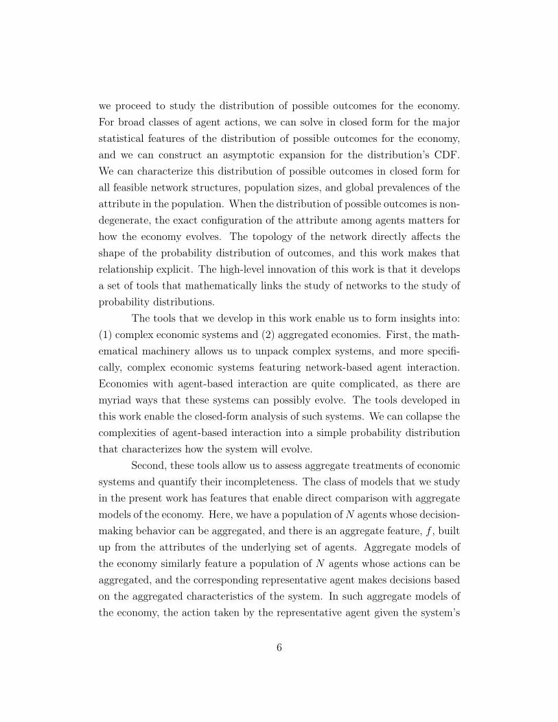
Imagine that we have an economy with an unemployment rate of tenpercent whose agents differ in their sentiments about the macroeconomy. Thesevariations in macroeconomic sentiment arise because the agents have differentlocal environments. In particular, the agents in the population are organizedon an observation network, and they form macroeconomic sentiment fromtheir local neighborhoods on the network. The top left of Figure 1 depicts thepopulation of agents and the underlying observation network, whose shadednodes indicate unemployment and whose network linkages indicate who ob-serves whom. If we focus on the two striped nodes in the top left of Figure 1,we see that the agent on the left-hand side is completely surrounded by unem-ployed agents, while the agent on the right-hand side is completely surroundedby agents who are gainfully employed; as a result, these two agents stronglydiffer in their levels of macroeconomic sentiment. These two very different localenvironments are consistent with the same overall economic fundamentals.

We can compute the level of aggregate macroeconomic sentiment inthe population by simply taking the population average of each agent’s locallyformed sentiment. Specifically, we determine the local unemployment rate foreach agent on the network, and we then compute the average local unemploy-ment rate in the population. Therefore, for a given configuration or allocation

1

Figure 1: Four configurations of unemployment for a population of agentsorganized on an observation network. Shaded (blue) nodes denote unemployedindividuals.

of unemployment among the agents in the population, we have a correspondingaverage local unemployment rate, which proxies for aggregate macroeconomicsentiment. Now suppose that we change which group of agents is unemployed(Figure 1, top right). The economy’s fundamentals stay the same, but thelevel of aggregate macroeconomic sentiment can change because we are poten-tially adjusting each agent’s local environment on the network. For all possibleconfigurations of unemployment in the population (Figure 1 features four suchconfigurations), we can compute a corresponding level of aggregate macroe-conomic sentiment. Given the overall unemployment rate, there is this entirerange of possible levels of aggregate macroeconomic sentiment; the topology ofthe underlying network shapes that range. In this work, we show how to mapthe topology of the underlying observation network to a probability distribu-tion of possible average local unemployment rates, which proxies for aggregatemacroeconomic sentiment. We introduce tools that enable us to compute inclosed-form all of the major statistical features of this probability distribution,and we develop a closed-form expression that essentially draws its CDF; wecan exactly specify how the topological features of the underlying observationnetwork shape this probability distribution.

By assuming that agents form macroeconomic sentiment from their

2

local unemployment rates, we are able to quantify the extent to which ag-gregate sentiment is positive or negative given the economy’s fundamentals;aggregate sentiment is positive, that is, there are waves of optimism, whenthe average local unemployment rate is less than the overall unemploymentrate, while aggregate sentiment is negative, that is, there are waves of pes-simism, when the average local unemployment rate is greater than the overallunemployment rate. We can moreover quantify this deviation in the averagelocal unemployment rate from the overall unemployment rate and thereforequantify deviations in aggregate sentiment away from the level that is com-mensurate with the economy’s fundamentals. We show how the underlyinginteraction structure among agents in the economy shapes the capacity forthere to exist these non-fundamental swings in aggregate sentiment for allpopulation sizes. We thus offer a mechanism for the formation of individualand aggregate macroeconomic sentiment that essentially microfounds animalspirits.

Now sentiment only matters if it somehow impacts agent decision-making. We therefore study a setting in which each agent’s locally formedmacroeconomic sentiment impacts that agent’s voting decision in an upcom-ing presidential election. With there being 137.5 million voters, the number ofvoters in the 2016 U.S. presidential election, we find that the variation in aggre-gate macroeconomic sentiment is sufficiently large that it can actually mimicvariations in business cycle conditions, and the election outcome accordinglydepends on the particular configuration of unemployment; the fundamentalsof the economy alone are insufficient for determining the election outcome.

The application focuses on observation networks and distributions ofaggregate macroeconomic sentiment and election outcomes. This applicationemerges from a more general theoretical framework, and the mathematicaltools employed in the application emerge from a more general set of theoreti-cal tools. In the more general setting, we have an economy with a populationof N agents, each of whom has a binary-valued attribute. There are n N

agents with the attribute’s unit value, so the global relative frequency of theattribute is f =

n

N

. These N agents are organized on a network, and each

3

networked agent’s decision-making depends on the local relative frequency ofthe attribute. Since agents have different positions on the network, they po-tentially have different local relative frequencies of the attribute arising fromdifferent network neighborhoods, and this can lead the agents to choose differ-ent actions. For each possible configuration of the attribute, we are interestedin the economy’s outcome. Depending on the environment, the outcome ofinterest might be the aggregate action in the population, it might be theaction of a particular individual, or it might be the outcome of an event,such as the election outcome that we study here. We construct a distribu-tion of possible outcomes by considering all

�

N

n

�

possible configurations of theattribute. Given the global relative frequency of the attribute and agents’decision-making behavior, we map the topology of the underlying network toa probability distribution of possible outcomes for the economy.

To carry out this mapping from underlying network to distributionof possible outcomes, we first must study the local relative frequency of theattribute. Holding fixed the attribute’s global relative frequency, for eachconfiguration there is an associated local relative frequency of the attribute.Therefore, given the attribute’s global relative frequency and the structure ofthe underlying network, we can construct an entire probability distribution ofpossible local relative frequencies of the attribute. We refer to the distributionof possible local relative frequencies of the attribute as a precursor distribu-tion because its construction precedes our construction of the distribution ofpossible outcomes for the economy. Once we have computed the precursor dis-tribution, we can then construct the distribution of possible outcomes for theeconomy given agents’ decision-making behavior. Our precursor distributioncharacterizes the extent to which the attribute’s local relative frequency devi-ates in either direction away from its global relative frequency. The capacityfor such variation in the attribute’s local relative frequency depends on the un-derlying network structure, and it determines the extent to which the outcomeof the economy can deviate from a benchmark outcome.1 When the probability

1The benchmark outcome is the one that results if we ignore the underlying configurationof the attribute and only take into account the attribute’s global relative frequency.

4

distribution of possible outcomes is non-degenerate, we consider the economicsystem to be configuration dependent. Configuration dependence enables theexistence of phenomena that would otherwise not emerge if we only consideredthe aggregate properties of the economy, such as the attribute’s global rela-tive frequency; it adds richness to our models of the economy because thereis an entire distribution of possible outcomes consistent with the aggregateproperties of the economy.

In this work, we develop tools so that we can characterize in closed formthe major statistical features of our precursor distribution for every feasiblenetwork structure, population size, and global prevalence of the binary-valuedattribute. We demonstrate how to construct an asymptotic expansion for theCDF of the precursor distribution, which explicitly shows how the network’stopology affects the shape of the precursor distribution. We determine thoseconditions and network topologies for which the local relative frequency ofthe attribute is invariant to configuration, which makes the precursor distri-bution degenerate and the outcome of the economy generally only dependenton the aggregate properties of the system. More generally, we show how tostatistically characterize the precursor distribution when every configuration isequally likely and when every configuration occurs with some arbitrary proba-bility. We can precisely determine how network primitives and other featuresof the underlying agent interaction network directly generate probability distri-butions with certain statistical properties. We establish a central limit theoremresult from which we can characterize the limiting behavior of the precursordistribution, and by extension, the distribution of possible outcomes for theeconomy as the network grows and the population size tends to infinity. Wedevelop a Berry-Esseen-type inequality that specifies the rate at which the cen-tral limit theorem result applies. We identify topological features of the agentinteraction network that make the precursor distribution and the distributionof possible outcomes for the economy approximately non-degenerate even insettings with very large population sizes and law of large numbers forces tryingto collapse these distributions.

Once we have characterized the precursor distribution in full generality,

5

we proceed to study the distribution of possible outcomes for the economy.For broad classes of agent actions, we can solve in closed form for the majorstatistical features of the distribution of possible outcomes for the economy,and we can construct an asymptotic expansion for the distribution’s CDF.We can characterize this distribution of possible outcomes in closed form forall feasible network structures, population sizes, and global prevalences of theattribute in the population. When the distribution of possible outcomes is non-degenerate, the exact configuration of the attribute among agents matters forhow the economy evolves. The topology of the network directly affects theshape of the probability distribution of outcomes, and this work makes thatrelationship explicit. The high-level innovation of this work is that it developsa set of tools that mathematically links the study of networks to the study ofprobability distributions.

The tools that we develop in this work enable us to form insights into:(1) complex economic systems and (2) aggregated economies. First, the math-ematical machinery allows us to unpack complex systems, and more specifi-cally, complex economic systems featuring network-based agent interaction.Economies with agent-based interaction are quite complicated, as there aremyriad ways that these systems can possibly evolve. The tools developed inthis work enable the closed-form analysis of such systems. We can collapse thecomplexities of agent-based interaction into a simple probability distributionthat characterizes how the system will evolve.

Second, these tools allow us to assess aggregate treatments of economicsystems and quantify their incompleteness. The class of models that we studyin the present work has features that enable direct comparison with aggregatemodels of the economy. Here, we have a population of N agents whose decision-making behavior can be aggregated, and there is an aggregate feature, f , builtup from the attributes of the underlying set of agents. Aggregate models ofthe economy similarly feature a population of N agents whose actions can beaggregated, and the corresponding representative agent makes decisions basedon the aggregated characteristics of the system. In such aggregate models ofthe economy, the action taken by the representative agent given the system’s

6

aggregate characteristics is often unique; when the representative agent makesa decision based on the global relative frequency of the attribute, there is a sin-gle benchmark outcome. However, once we account for the underlying networkstructure, we see that there is actually an entire non-degenerate distributionof possible outcomes for the economy consistent with the attribute’s globalrelative frequency. Using the tools developed in this work, we can introduce aconfigurational error bound and place that error bound about the benchmarkoutcome of the simpler aggregate economy to account for this multiplicity ofpossible outcomes. The size of the error bound depends on the topology of theunderlying network in the system. By incorporating this error bound, we allowfor a more complete and a more nuanced understanding of the phenomena thataggregate models of the economy seek to study. As a result, two systems withthe same aggregate features can evolve differently due to differences in theirunderlying configurations; the error bound that we construct accounts for thisvariation in the two economic outcomes relative to each other and relative tothe benchmark outcome.

1.1 Relation to the Literature

This work interfaces with the literature on: (1) complex economic sys-tems, (2) networks, (3) aggregation, and (4) macroeconomic sentiment. Re-search in the area of complex economic systems includes Granovetter (1978),Brock and Durlauf (2001), Bisin et al. (2004), and Horst and Scheinkman(2004). The present work contributes to that literature by shifting the theoret-ical object of interest away from a unique equilibrium outcome to a probabilitydistribution of possible outcomes.

In the area of networks, recent papers include Gale and Kariv (2003),Golub and Jackson (2010), Acemoglu, Ozdaglar, and ParandehGheibi (2010),Acemoglu, Dahleh, Lobel, and Ozdaglar (2011), Banerjee, Breza, Chandra-sekhar, and Mobius (2016), Harel et al. (2018), and Chandrasekhar, Larreguy,and Xandri (2019). The present work contributes to research on networks bydeveloping a set of theoretical tools that map networks to probability distri-

7

butions in the economy. This set of tools is much more extensive than anyexisting set of tools. In macroeconomics, existing work focuses on the distri-bution of output, and in the area of social learning, existing work focuses onlearning the truth. The set of tools developed in the present work can be ap-plied to a much broader set of networks and distributions in the economy, notjust production networks and output, for example. Also, much of the existingwork only studies the relationship between networks and the first or secondmoments of the corresponding probability distribution in the asymptotic casewith infinite population size. There is a focus on the rate at which the lawof large numbers applies as the population size grows to infinity. Meanwhile,we study networks at all population sizes and we can characterize both lower-order and higher-order distributional features. We have results that show howto develop closed-form expressions that essentially draw the CDFs of proba-bility distributions for any population size and feasible network.

Research in the area of aggregation tends to examine whether aggregatefluctuations in output can arise from micro-level shocks, or if an aggregateparameter is needed in models of the macroeconomy to generate sufficientlysizable aggregate fluctuations. Papers include Bak, Chen, Scheinkman, andWoodford (1993), Scheinkman and Woodford (1994), Horvath (1998, 2000),Gabaix (2011), and Acemoglu, Carvalho, Ozdaglar, and Tahbaz-Salehi (2012).These papers offer different mechanisms that slow the rate at which the law oflarge numbers applies. They study the role of sectoral production networks,granularity in firm size, and non-convexities in production technologies coupledwith local interaction among sectors in generating adequate fluctuations inoutput that persist even as the economy becomes increasingly disaggregated.Recently, research in this area has also been trying to study how microeconomicshocks shape the higher-order features of the output distribution; recent workincludes Acemoglu, Ozdaglar, and Tahbaz-Salehi (2017) and Baqaee and Farhi(2018). The present work tackles this issue of aggregation as well. It examinesthe extent to which the distribution of possible outcomes for the economyremains non-degenerate in a large-N setting. We develop theoretical resultsthat characterize the variance and the CDF of this distribution, including its

8

higher-order features, for every possible population size and network topology,including the limit as N ! 1. We can explicitly examine how the topologicalfeatures of the interaction network shape the capacity for the distribution ofoutcomes for the economy to remain approximately non-degenerate, even forlarge N .

Recent research in the area of macroeconomic sentiment includes Barskyand Sims (2012), Angeletos and La’O (2013), Benhabib, Wang, and Wen(2015), Huo and Takayama (2015), Milani (2017), Acharya, Benhabib, andHuo (2018), and Angeletos, Collard, and Dellas (2018). The present workinteracts with the existing literature on macroeconomic sentiment by provid-ing a simple mechanism for the formation of macroeconomic sentiment amongagents. This mechanism allows us to quantify the extent to which individualsentiment and aggregate sentiment deviate from a level that is commensuratewith economic fundamentals. The present work also shows how the underly-ing interaction structure among agents shapes the capacity for there to existnon-fundamental swings in aggregate sentiment. Through this work, we aremicrofounding sentiment shocks.

1.2 Outline of Paper

Section 2 provides notation and definitions, and it develops both thetheoretical framework for the application, featuring two examples, and themore general theoretical framework. Sections 3 and 4 introduce a large set oftheoretical results that statistically characterize the precursor distribution, andby extension, the distribution of possible outcomes for the economy given thetopology of agents’ interaction network. Section 3 mainly focuses on the casein which each configuration of the attribute is equally likely, while Section 4relaxes this assumption. Section 5 applies all of these theoretical results tostudy how agent interaction networks shape distributions of aggregate macroe-conomic sentiment and election outcomes for fixed economic fundamentals ina large-population setting. Section 6 shows, more generally, how to map thetopologies of agent interaction networks to distributions of possible outcomes

9

for the economy given agent actions. Section 7 concludes.

2 Theoretical Framework

2.1 Notation and Definitions

The cardinality of a set X is |X |. A multiset is an object similar to aset, but it allows for multiple instances of each of its elements. Vector x is acolumn vector by default. The ith element of vector x is x

i

or [x]

i

. The ijth

element of matrix X is [X]

ij

, the ith row of X is [X]

i⇤, and the jth column of Xis [X]⇤j. The column vector whose elements all equal 1 is 1, and the unit vectorb

u

i

has [

b

u

i

]

j

= 1 for i = j and [

b

u

i

]

j

= 0 otherwise. Matrix X is row-stochasticif X1 = 1 and all matrix elements of X are non-negative. Matrix X is doublystochastic if it is both row-stochastic and column-stochastic, that is, X1 = 1,X

T

1 = 1, and all matrix elements of X are non-negative. Non-negative matrixX is primitive if there exists an integer q � 1 such that [Xq

]

ij

> 0 for all matrixelements in X

q. Graph G is an ordered pair G = (V , E) consisting of a set ofvertices (nodes) V and a set of edges E . (x, y, e

x,y

) 2 E is an edge between nodesx and y with weight e

x,y

. If the graph is directed, the edge is oriented fromx to y; otherwise, the edge is not oriented. G �¯X� refers to a weighted graphwith weighted adjacency matrix ¯

X, whose non-zero elements are⇥

¯

X

⇤

ij

= ei,j

.

2.2 Theoretical Framework for Application

We begin this section by developing the theoretical framework for ourapplication of interest and working through two examples. We conclude thissection by developing the more general theoretical framework that nests thisparticular application as well as many other applications.

The theoretical preliminaries for our application are as follows. Wehave a population of N agents. Each agent i has a binary-valued attribute, b

i

,that denotes employment status. Agent i has b

i

= 1 if he is unemployed, andotherwise b

i

equals zero. There are n unemployed agents in the population.The global unemployment rate is f =

n

N

. Given the overall unemployment

10

rate, there is a particular configuration, b (N, n), of unemployment in thepopulation:

Definition 1 A configuration b ⌘ b (N, n) of a binary-valued attribute in apopulation of N agents is an allocation of the attribute so that b

i

2 {0, 1} forevery agent i 2 {1, . . . , N} and b

T

1 = n.

The N⇥1 configuration vector b stacks the employment statuses of all agents,and it identifies the indices of those agents who are unemployed. We denoteB (N, n) as the set of all possible configurations of unemployment given f =

n

N

,and |B (N, n)| = �

N

n

�

.The N agents in the population are organized on a social observation

network, G �¯A�, with corresponding weighted adjacency matrix ¯

A. This net-work is directed, and the edges on the network indicate the direction of obser-vation.

⇥

¯

A

⇤

ij

= ei,j

means that agent i observes agent j and accords weight ei,j

to that observation. Agents place non-negative weight on each of their observa-tions, and we assume that the sum of all of these weights for a particular agentequals 1; matrix ¯

A is therefore row-stochastic. Each agent computes the localunemployment rate from his position on the network. The population vector oflocal unemployment rates, bf

�

¯

A,b, N, n�

, is then: bf�

¯

A,b, N, n�

=

¯

Ab (N, n).For a given configuration of unemployment, the average local unemploymentrate, bf

avg

�

¯

A,b, N, n�

, is:

bfavg

�

¯

A,b, N, n�

=

1

N1

T

b

f

�

¯

A,b, N, n�

=

1

N1

T

¯

Ab (N, n) =⇥

d

�w

�

¯

A

�⇤

T

b (N, n) .

We see that bfavg

�

¯

A,b, N, n�

is the product of a configuration vector, b (N, n),and a vector of agent weights, specifically, a vector of average weighted in-degrees for the graph G �¯A�: d�

w

�

¯

A

�

=

1N

¯

A

T

1. The greater an agent’s averageweighted in-degree, the greater the observability of that agent in the popula-tion, and the greater the contribution to the average local unemployment rateif that agent is unemployed. We are interested in constructing the distributionof possible average local unemployment rates for a given observation networkand overall unemployment rate. We accordingly introduce the random vari-

11

able bFavg

�

¯

A, N, n�

whose realizations are configuration-specific average localunemployment rates, bf

avg

�

¯

A,b, N, n�

. Corresponding to this random variableare the CDF G b

Favg(A,N,n

)

(t) and the PMF g bFavg(A,N,n

)

(t). Assuming that eachconfiguration of unemployment is equally likely,

G bFavg(A,N,n

)

(t) =1

|B (N, n)|X

b(N,n)2B(N,n)

1 bfavg(A,b,N,n

)

t

.

We can imagine that agents form macroeconomic sentiment from their localunemployment rates, so G b

Favg(A,N,n

)

(t) proxies for aggregate macroeconomicsentiment.

2.3 Two Examples

In the next two examples, we study how the topology of agents’ inter-action network shapes the distribution of possible average local unemploymentrates.

Example 1 (Average Local Unemployment Rate, N = 4) Consider aneconomy with N = 4 agents and an unemployment rate of f = 0.25. Agents’social observation network, G �¯A�, has the weighted adjacency matrix depictedimmediately below. Assuming each configuration of unemployment is equallylikely, we can compute the distribution, g b

Favg(A,N,n

)

(t), of possible average localunemployment rates:

¯

A =

0

B

B

B

B

@

1/4 1/4 1/4 1/4

0

1/3 1/3 1/3

0 0

1/2 1/2

0 0 0 1

1

C

C

C

C

A

g bFavg(A,N,n

)

(t) =

8

>

>

>

>

>

>

<

>

>

>

>

>

>

:

0.25 if bFavg

�

¯

A, N, n�

= 0.0625

0.25 if bFavg

�

¯

A, N, n� ⇡ 0.146

0.25 if bFavg

�

¯

A, N, n� ⇡ 0.271

0.25 if bFavg

�

¯

A, N, n� ⇡ 0.521

.

In this example, there are four configurations of unemployment in theeconomy consistent with f = 0.25: bu1, bu2, bu3, and b

u4 2 R4 (see Figure 2). Foreach configuration, we can compute the average local unemployment rate:

12

0 0.1 0.2 0.3 0.4 0.5 0.60

0.25

0.5

0.75

1

Probability

Figure 2: The four possible configurations of unemployment (left), and theprobability distribution, g b

Favg(A,N,n

)

(t), of possible average local unemploy-ment rates (right).

For b =

b

u1, bf�

¯

A,b, N, n�

=

⇣

0.25 0 0 0

⌘

T

and bfavg

= 0.0625.

For b =

b

u2, bf�

¯

A,b, N, n�

=

⇣

0.25 0.33 0 0

⌘

T

and bfavg

⇡ 0.146.

For b =

b

u3, bf�

¯

A,b, N, n�

=

⇣

0.25 0.33 0.50 0

⌘

T

and bfavg

⇡ 0.271.

For b =

b

u4, bf�

¯

A,b, N, n�

=

⇣

0.25 0.33 0.50 1

⌘

T

and bfavg

⇡ 0.521.

From these values, we can then construct the distribution g bFavg(A,N,n

)

(t) inFigure 2.

We see that the topology of agents’ observation network generates widevariation in individual agents’ local unemployment rates for a particular con-figuration of unemployment in the economy, and it generates variation in in-dividual agents’ local unemployment rates across configurations. The lattervariation arises from agents having different levels of observability. Agent 1has a low average weighted in-degree, and therefore a low agent weight andpoor observability, so when he is unemployed, agents 1, 2, 3, and 4 respectivelyhave local unemployment rates of 25 percent, 0 percent, 0 percent, and 0 per-cent; agent 4 meanwhile has a high average weighted in-degree, and therefore ahigh agent weight and strong observability, so when he is unemployed, agents1, 2, 3, and 4 respectively have local unemployment rates of 25 percent, 33percent, 50 percent, and 100 percent. This variation in agents’ observabil-ity causes the average local unemployment rate to change with configuration.When agent 1 is unemployed, the average local unemployment rate is 6.25

13

percent, while when agent 4 is unemployed, the average local unemploymentrate is 52.1 percent. These values for the average local unemployment rate alsostrongly deviate from the actual unemployment rate of 25 percent. If agentsform macroeconomic sentiment from their local rates of unemployment, thendepending on the particular configuration of unemployment in the economy,agents on average might feel that the economy is doing much better or muchworse than its fundamentals might otherwise suggest.

0 0.1 0.2 0.3 0.4 0.5 0.6 0.7 0.8 0.9 10

0.1

0.2

0.3

0.4

0.5

0.6

0.7

0.8

0.9

1

(A)

(B)

(C)

(D)

45-Degree Marker

Figure 3: Possible average local unemployment rates, bfavg

�

¯

A,b, N, n�

, giventhe global unemployment rate, f , and potential pathways (A-D) for the averagelocal unemployment rate as the global unemployment rate evolves.

As illustrated in Figure 3, we can trace different pathways for theaverage local unemployment rate as the global unemployment rate evolves.Changes in configuration can accommodate different phenomena that wouldotherwise not emerge from just the aggregate properties of the system. Path (B)illustrates how there can be dramatic swings in sentiment for a small adjust-ment to the economy’s fundamentals; as the unemployment rate increases from25 percent to 50 percent, there is a 72.9-percentage-point increase in the aver-age local unemployment rate. Path (C) illustrates how sentiment can move ina direction opposite to that of fundamentals. Even though the unemploymentrate is declining from 50 percent to 25 percent, the average local unemploy-ment rate increases 31.3 percentage points. The decrease in unemploymentwould suggest that the economy is improving, but the agents in the popula-tion on average locally observe the economy to be worsening. Paths (A) and

14

(D) illustrate hysteresis within the economy.

Example 2 (Average Local Unemployment Rate, N = 15) Consideran economy with N = 15 agents and an unemployment rate of f = 0.20. Thelinkages for the social observation network are formed from preferential attach-ment, as depicted in Figure 4, and every node also has a self-loop. We assumethat agents assign an equal weight to each of their observations, which makesthe underlying observation network G �¯A� a weighted directed graph. Assum-ing that each configuration of unemployment in the economy is equally likely,the distribution of possible average local unemployment rates, g b

Favg(A,N,n

)

(t),is on the right-hand side of Figure 4.

1 2 3 4 5 6 7 8 9 10 11 12 13 14 15Node

0

0.05

0.1

0.15

0.2

Ave

rage

Wei

ghte

d In

-Deg

ree

Figure 4: For Example 2, network linkages formed from preferential at-tachment with self-loops for every node (left). Average weighted in-degrees(middle), d�

w

�

¯

A

�

, and the distribution of average local unemployment rates,g bFavg(A,N,n

)

(t) (right).

In this second example, there are�

153

�

= 455 possible configurations ofthe unemployment attribute among agents in the population consistent with a20-percent unemployment rate. We compute the average local unemploymentrate configuration by configuration, and we then construct the accompanyingprobability distribution. We observe substantial heterogeneity in agents’ av-erage weighted in-degrees, d�

w

�

¯

A

�

=

1N

¯

A

T

1, as can be viewed in the middleof Figure 4. As a result, the probability distribution of possible average lo-cal unemployment rates has sizable variance. For a 20-percent unemploymentrate, the average local unemployment rate can vary from 11.9 percent to 33.1percent.

15

0 0.1 0.2 0.3 0.4 0.5 0.6 0.7 0.8 0.9 10

0.10.20.30.40.50.60.70.80.9

145-Degree Marker

10.90.80.70 0.60 0.50.1 0.2 0.40.3

0.1

0.4 0.30.5

Prob

abili

ty

0.20.6 0.7

0.2

0.10.8 0.9 01

0.3

45-Degree Marker

Figure 5: Possible average local unemployment rates, bfavg

�

¯

A,b, N, n�

, for agiven global unemployment rate, f , (left). Probability distribution of possi-ble average local unemployment rates, g b

Favg(A,N,n

)

(t), for each global level ofunemployment (right).

We can construct such a probability distribution of possible average lo-cal unemployment rates configuration by configuration for every feasible levelof unemployment in this economy. Figure 5 plots the set of possible averagelocal unemployment rates for a fixed global unemployment rate, and it alsoplots the corresponding probability distribution of possible average local unem-ployment rates for each feasible global level of unemployment in the economy.When one agent is unemployed, there are just 15 possible configurations, whilewhen 7 or 8 agents are unemployed, there are 6435 possible configurations. Asthe population size increases, the total number of configurations,

�

N

n

�

, growscombinatorially, and it no longer becomes feasible to construct the distributionof possible average local unemployment rates configuration by configuration.In Section 3, we present a set of theoretical results that allows us to constructthis probability distribution and compute its statistical features in closed formfor every population size, every feasible unemployment rate, and every under-lying social observation network structure.

We can imagine that agents form sentiment about the macroeconomyfrom their local environments on the network. Each agent’s local unemploy-ment rate therefore shapes individual macroeconomic sentiment, and the av-erage local unemployment rate shapes aggregate macroeconomic sentiment.

16

Now, sentiment only matters if it impacts agent decision-making. Therefore,our application, which is more extensively developed in Section 5, studies asetting in which each agent’s locally formed macroeconomic sentiment impactsthat agent’s voting decision in an upcoming presidential election. Aggregatevoting behavior depends on aggregate macroeconomic sentiment. If aggregatemacroeconomic sentiment sufficiently varies with which group of agents is un-employed, we can potentially have more than one possible election outcomefor the same underlying set of fundamentals. Through this application, wemap the topology of agents’ social observation network, first, to a probabil-ity distribution of possible levels of aggregate macroeconomic sentiment giventhe overall unemployment rate, and next, we map the distribution of aggre-gate macroeconomic sentiment to a probability distribution of possible electionoutcomes given agents’ voting behavior. This application studies how agentinteraction networks shape election outcomes.

2.4 General Theoretical Framework

The application in this work focuses on social observation networks,aggregate macroeconomic sentiment, and election outcomes, but the theoreti-cal framework and the accompanying set of tools are much more general. Thetheoretical tools developed in this work allow us to map the topologies of net-works in the economy to different probability distributions of interest. We nowintroduce the set of theoretical preliminaries for the more general framework.There is a one-to-one correspondence between the theoretical preliminaries forthe application and the theoretical preliminaries for the more general setting.In the more general setting, we have a population of N agents organized on anetwork G �¯A� whose weighted adjacency matrix ¯

A is row-stochastic.2 Eachagent i has a binary-valued attribute, b

i

. There are n agents that have theattribute’s unit value. The global relative frequency of the attribute in thepopulation is f =

n

N

. Each agent makes a decision based on the local relativefrequency of the attribute. Consistent with f , there are combinatorially many

2Schlossberger (2018) relaxes the assumption that the weighted adjacency matrix cor-responding to the agent interaction network must be row-stochastic.

17

possible configurations b (N, n) 2 B (N, n), |B (N, n)| = �

N

n

�

, of the attributeamong agents. Given the underlying network, the global relative frequencyof the attribute, and agents’ decision-making behavior, we are interested inthe distribution of possible outcomes for the economy. We are essentially re-arranging attributes among the agents in the population and computing theeffect on the economy’s outcome.

In the application, to go from network to probability distribution, westart off with the underlying observation network G �¯A�. Given the global un-employment rate, f , we compute an intermediate probability distribution: thedistribution of possible average local unemployment rates, G b

Favg(A,N,n

)

(t). Werefer to G b

Favg(A,N,n

)

(t) as a precursor distribution because its construction pre-cedes the construction of the distribution of possible election outcomes. Giventhe precursor distribution and agents’ voting behavior, we then construct thedistribution of possible election outcomes.

In the general setting, to go from network to probability distribution,we start off with the underlying network G �¯A�. Given the global relativefrequency of the attribute, f , we compute a distribution of possible local rel-ative frequencies of the attribute. The topology of the underlying networkdetermines the extent to which the local relative frequency of the attributecan deviate from its global relative frequency, and that determines the extentto which we can have variation in the economy’s outcome. Then, given thisprecursor distribution and agents’ decision-making behavior, we construct thedistribution of possible outcomes for the economy.

There is a one-to-one mapping from the construction of the precursordistribution in the application and the construction of the precursor distribu-tion in the more general setting. For the application, we take the followingapproach: we derive an N ⇥ 1 vector of agent weights, or more precisely, avector of average weighted in-degrees, d�

w

�

¯

A

�

, from the underlying social ob-servation network. Given the overall unemployment rate, f , for each feasibleconfiguration of unemployment, we compute the average local unemploymentrate as follows: bf

avg

�

¯

A,b, N, n�

=

⇥

d

�w

�

¯

A

�⇤

T

b (N, n). We are interestedin the distribution of possible average local unemployment rates, so we intro-

18

duce the random variable bFavg

�

¯

A, N, n�

with configuration-specific realizationbfavg

�

¯

A,b, N, n�

, CDF G bFavg(A,N,n

)

(t), and PMF g bFavg(A,N,n

)

(t).In the more general theoretical setting, we take the following approach:

we derive an N ⇥ 1 vector of agent weights, w�

¯

A

�

, from the underlying net-work. Given the attribute’s global relative frequency, f , for each feasibleconfiguration of the attribute, we compute the local relative frequency of theattribute, x

�

¯

A,b, N, n�

, as follows: x�

¯

A,b, N, n�

=

⇥

w

�

¯

A

�⇤

T

b (N, n). Weare interested in the distribution of possible local relative frequencies of theattribute, so we introduce the random variable X

�

¯

A, N, n�

with configuration-specific realization x

�

¯

A,b, N, n�

, CDF GX

(

A,N,n

)

(t), and PMF gX

(

A,N,n

)

(t).Assuming that each configuration of the attribute among agents is equallylikely:

GX

(

A,N,n

)

(t) =1

|B (N, n)|X

b(N,n)2B(N,n)

1x

(

A,b,N,n

)

t

.

3 Characterizing the Precursor Distribu-

tion: Statistical Features of X�

¯

A, N, n�

We now characterize the precursor distribution, GX

(

A,N,n

)

(t). We focuson this distribution rather than the distribution of possible outcomes for theeconomy because the latter distribution depends on agents’ decision-makingbehavior. Accordingly, we characterize the precursor distribution, and thenfor a specific set of agent decision-making rules, we can construct the corre-sponding distribution of possible outcomes for the economy. We are able tocharacterize the precursor distribution for all population sizes, all prevalencesof the attribute in the population, and all feasible underlying networks. Thetopological features of agent interaction networks shape the statistical featuresof the precursor distribution, and by extension, the distribution of possible out-comes for the economy. We map the topology of agents’ interaction network,G �¯A�, to a network-derived vector of agent weights, w

�

¯

A

�

, and we then mapthe network-derived vector of agent weights to the probability distribution,

19

GX

(

A,N,n

)

(t).3 Many of the theoretical results assume that each configurationof the attribute is equally likely, although this is an assumption that we relaxin Section 4.

We start off by identifying the null case in which GX

(

A,N,n

)

(t) is de-generate. Such degeneracy arises when the local relative frequency of theattribute, x

�

¯

A,b, N, n�

, remains the same for all configurations b 2 B (N, n).When this condition holds for every feasible f , quantity x

�

¯

A,b, N, n�

is in-variant to configuration:

Definition 2 Quantity x�

¯

A,b, N, n�

is invariant to configuration whenx�

¯

A,b, N, n�

= x�

¯

A,b0, N, n�

for all configurations b,b0 2 B (N, n), andthis property holds for all feasible n.

When x�

¯

A,b, N, n�

is invariant to configuration, the support of X�

¯

A, N, n�

takes one value. In the next theorem, we determine the necessary and sufficientrestrictions on the vector of agent weights, w

�

¯

A

�

, for x�

¯

A,b, N, n�

to beinvariant to configuration, and we solve for the support of X

�

¯

A, N, n�

:

Theorem 1 Scalar quantity x�

¯

A,b, N, n�

=

⇥

w

�

¯

A

�⇤

T

b (N, n) is invariantto configuration if and only if

⇥

w

�

¯

A

�⇤

i

=

1N

for all i 2 {1, . . . , N}. Whenx�

¯

A,b, N, n�

is invariant to configuration, x�

¯

A,b, N, n�

=

n

N

.

All proofs from the main text are in Appendix A of the Supplementary Ma-terials. When w

�

¯

A

�

=

1N

1, every agent has the same effective representationin the population. As a result, the local relative frequency of the attributeis always equal to the attribute’s global relative frequency, f ; the support ofX�

¯

A, N, n�

is f . Generally speaking, in this null environment, the particularconfiguration of the attribute among agents becomes irrelevant for how thesystem evolves. The outcome of the economy only depends on the system’saggregate feature, f .4 The conditions for degeneracy are quite restrictive, so

3The theoretical results that we later develop hold even when the vector of agent weightsis not network-derived. See Schlossberger (2019).

4Applying this theoretical result to our application, we find that the distribution ofaverage local unemployment rates, bFavg

�

¯

A, N, n�

, is degenerate when d

�w

�

¯

A

�

=

1N 1, that

is, when the weighted adjacency matrix ¯

A for the social observation network is doublystochastic.

20

most economic systems with interacting agents tend to have probability distri-butions that feature some level of non-degeneracy, which makes the outcomeof the economy configuration-dependent.

We proceed to characterize the statistical features of the precursor dis-tribution in the more general setting. To simplify mathematical expressions inlater theorems, we define random variable W

�

¯

A

�

with realization⇥

w

�

¯

A

�⇤

i

,the weight for agent i.5 For the application, we introduce random variableD�

w

�

¯

A

�

with realization⇥

d

�w

�

¯

A

�⇤

i

. We begin by defining the first moment ofX�

¯

A, N, n�

:

Theorem 2 EX�

¯

A, N, n�

=

n

N

= f .

The first moment of X�

¯

A, N, n�

is equal to the attribute’s global relative fre-quency, f . The local relative frequency of the attribute can deviate in eitherdirection away from the attribute’s global relative frequency, but in expecta-tion, it must equal this value. The distribution of X

�

¯

A, N, n�

is consequentlycentered about the point in which configuration is irrelevant and only theaggregate feature, f , matters. This relationship between EX

�

¯

A, N, n�

andf generally disappears once each configuration is no longer equally likely tooccur. We can use the theoretical results developed in this section to charac-terize the statistical features of bF

avg

�

¯

A, N, n�

; we simply substitute the triplet�

X�

¯

A, N, n�

,W�

¯

A

�

,w�

¯

A

��

with the triplet⇣

bFavg

�

¯

A, N, n�

, D�w

�

¯

A

�

,d�w

�

¯

A

�

⌘

.We proceed to study the second moment of X

�

¯

A, N, n�

. Assumingthat each configuration is equally likely, the variance of X

�

¯

A, N, n�

and itslimiting behavior as N ! 1 are:

Theorem 3 VarX�

¯

A, N, n�

=

n

N

�

1� n

N

�

N

N�1

�

N VarW�

¯

A

��

. By introduc-ing replica graphs to scale up the population, VarX

�

¯

A, N, n� ! 0 at rate N�1

as N ! 1.5The distribution GX

(

A,N,n)

(t) strongly depends on the distributional features ofagents’ weights. We can see this relationship most clearly when n = 1. For that case,GX

(

A,N,n)

(t) = GW(

A)

(t), and the distribution of possible local relative frequencies of theattribute equals the distribution of agent weights.

21

The variance of the precursor distribution directly depends on the populationvariance of agent weights. If there is large heterogeneity in agents’ weights,then the local relative frequency of the attribute strongly varies with con-figuration. To study the behavior of VarX

�

¯

A, N, n�

as the population in-creases in size, introduce replica graphs that both preserve existing agents’relative weights and maintain the amount of weight accorded to a particularindexed node on the graph. By scaling the population upwards in this manner,VarX

�

¯

A, N, n�

halves as the population size doubles. Appendix C identifiesthe vector of agent weights for which VarX

�

¯

A, N, n�

is maximal.Since agents choose actions based on some local relative frequency of the

attribute, the variance of the precursor distribution captures how dependentthe outcome of the economy is on the underlying configuration of the attribute.We can use the closed-form expression for VarX

�

¯

A, N, n�

in Theorem 3 toconstruct error bounds that account for the range of possible outcomes and/orpaths for aggregated networked economies. These bounds quantify the extentto which there can be variation in the outcome of an economy holding fixedits aggregate properties.

In the next theorem, we show how to compute the lower and upperbounds on the support of X

�

¯

A, N, n�

. These values represent the lowest andhighest possible local relative frequencies of the attribute given the attribute’sglobal relative frequency in the population. They determine the maximalextent to which the local relative frequency of the attribute can deviate fromits global relative frequency given the structure of the network. From thesevalues, we are able to bound the distribution of possible outcomes for theeconomy.

Theorem 4 Construct the ordered multiset {ws

}Ns=1 from the elements of

w

�

¯

A

�

so that ws

ws

0 whenever s s0. The lower and upper bounds on thesupport of X

�

¯

A, N, n�

are respectively:

min supp X�

¯

A, N, n�

=

n

X

s=1

ws

and max supp X�

¯

A, N, n�

=

N

X

s=N�n+1

ws

.

22

The lower bound on the support of X�

¯

A, N, n�

is equal to the sum of the n

smallest agent weights in the population, while the upper bound is equal tothe sum of the n largest agent weights in the population.

We proceed to study the limiting behavior of GX

(

A,N,n

)

(t) as N ! 1.To do so, we define the quantity

N

(✏) =1

P

N

i=1

�⇥

w

N

�

¯

A

�⇤

i

� 1N

�2

X

j2{1,...,N} s.t.���[

wN(A)]j� 1

N

���>✏�N

✓

⇥

w

N

�

¯

A

�⇤

j

� 1

N

◆2

where �N

=

⇣

n

N

�

1� n

N

�

P

N

i=1

�⇥

w

N

�

¯

A

�⇤

i

� 1N

�2⌘1/2

. We make the popula-tion size, N , explicit for the N ⇥ 1 vector w

N

�

¯

A

�

of network-derived agentweights because we wish to study the behavior of G

X

(

A,N,n

)

(t) as N increases.We establish the following central limit theorem-type result:

Theorem 5 If limN!1

N

(✏) = 0 for any ✏ > 0, then lim

N!1 GX(A,N,n)� nN

�N

(t)

= � (t) for all real t, where � (·) is the standard normal CDF.

The requirement that lim

N!1 N

(✏) = 0 for any ✏ > 0 is a Lindeberg-type condition. As the population size increases and the number of agentweights increases, the Lindeberg-type condition requires that there cannotbe any subset of agent weights as N ! 1 that strongly deviates from theaverage agent weight. When this condition holds, we informally have thatlim

N!1 GX

(

A,N,n

)

(t) ⇡ �

⇣

t� nN

�N

⌘

. The distribution of weighted local relativefrequencies of the attribute is asymptotically normal with mean f and variance�2N

, the mean of X�

¯

A, N, n�

and the variance of X�

¯

A, N, n�

. As the pop-ulation size increases, provided that the set of agent weights is well-behaved,the population variance of agent weights tends to zero, so VarX

�

¯

A, N, n�

also tends to zero. From this theoretical result, we see that the particularconfiguration of the attribute among agents becomes less relevant for how theeconomy evolves as N ! 1. The aggregate properties of the system, namelyf , start becoming sufficient.

The next theorem provides insight into the rate at which X�

¯

A, N, n�

23

converges to a normal distribution as the population size increases. It placesan upper bound on the maximal distance of the distribution G

X

(

A,N,n

)

(t) toa normal distribution with the same mean and variance:6

Theorem 6�

�

�

GX

(

A,N,n

)

(t)� �

⇣

t� nN

�N

⌘

�

�

�

CqnN (1�

nN )

PNi=1|[wN(A)]i

� 1N |3⇣PN

i=1([wN(A)]i� 1

N )2⌘3/2

for all real t, where C is an absolute constant.

The upper bound depends on f and the normalized third absolute momentfor the distribution of agent weights. It is a Berry-Esseen-type inequality thatspecifies the rate at which convergence to the normal distribution takes placeby bounding the maximal error of approximation.

Beyond the statistical features of X�

¯

A, N, n�

provided thus far, weare also interested in the CDF of the distribution, G

X

(

A,N,n

)

(t). The nextresult shows, via asymptotic expansion, how we can essentially draw the CDFof our distribution for any feasible population size, network structure, andprevalence of the attribute in the population. Let’s begin by defining thefunction J

�

¯

A, N, n, t�

:

J�

¯

A, N, n, t�

= � (t)�H2 (t)� (t)C1

N

X

i=1

bw3i

�H3 (t)� (t)

"

C2

N

X

i=1

bw4i

� 3

N

!

� 1

4N

#

�H5 (t)� (t)C3

N

X

i=1

bw3i

!2

,

where bwi

=

[

w(

A)]

i�EW

(

A)q

N VarW(

A)

, C1 =1� 2n

N

6(

nN (1�

nN ))

1/2 , C2 =1�6

(

nN )(1�

nN )

24(

nN )(1�

nN )

,

C3 =

(

1� 2nN )

2

72(

nN )(1�

nN )

, � (t) = �

0(t) = 1p

2⇡e�

t2

2 , and Hi

(t)� (t) = (�1)

i

d

i

dt

i � (t).Quantity bw

i

is constructed from the set of agent weights. We can then ap-proximate GX(A,N,n)�EX(A,N,n)

(VarX(A,N,n))1/2(t) by the function J

�

¯

A, N, n, t�

:

6Here, we take N to be large enough so that VarX�

¯

A, N, n�

=

nN

�

1� nN

�

NN�1

�

N VarW�

¯

A

��

=

nN

�

1� nN

�

NN�1

PNi=1

�⇥

wN

�

¯

A

�⇤

i� 1

N

�2 ⇡nN

�

1� nN

�

PNi=1

�⇥

wN

�

¯

A

�⇤

i� 1

N

�2= �2

N .

24

Theorem 7 Provided that condition (c) holds,

�

�

�

�

�

GX(A,N,n)�EX(A,N,n)

(VarX(A,N,n))1/2(t)� J

�

¯

A, N, n, t�

�

�

�

�

�

< C4 ⇥N

X

i=1

| bwi

|5

for all t, where C4 is only a function of n

N

.

Condition (c) (Robinson (1978)) Given C 0 > 0, there exist ✏ > 0, C > 0,and � > 0 not depending on N such that, for any fixed t, the number ofindices j, for which | bw

j

bx� t� 2r⇡| > ✏, for all

bx 2✓

C 0[ max

i

| bwi

| ]�1 , Ch

P

N

i=1 | bwi

|5i�1

◆

and all r = 0,±1,±2, . . . , is

greater than �N , for all N .

The asymptotic expansion J�

¯

A, N, n, t�

in Theorem 7 is to order 1/N . Condi-tion (c) requires that the multiset { bw

i

}Ni=1 not be clustered around too few val-

ues; it therefore also requires that the multiset of agent weights�⇥

w

�

¯

A

�⇤

i

N

i=1

not be clustered around too few values. This asymptotic expansion is ageneral result that enables us to very strongly approximate the distribution,G

X

(

A,N,n

)

(t):

GX

(

A,N,n

)

(t) ⇡ J

¯

A, N, n,t� EX

�

¯

A, N, n�

�

VarX�

¯

A, N, n��1/2

!

.

The function J�

¯

A, N, n, t�

is a collection of terms; the first term is the nor-mal distribution, and the other terms represent deviations away from thenormal distribution provided that they are non-zero. Note that

P

N

i=1 bw3i

=

N�1/2SkewW

�

¯

A

�

andP

N

i=1 bw4i

� 3N

= N�1 ⇥ �

Excess KurtosisW�

¯

A

��

. Ac-cordingly, we can re-write the function J

�

¯

A, N, n, t�

in terms of the higher-

25

order moments of W�

¯

A

�

:

J�

¯

A, N, n, t�

= � (t)�H2 (t)� (t)C1N�1/2

SkewW�

¯

A

�

�H3 (t)� (t)

C2

�

N�1Excess KurtosisW

�

¯

A

��� 1

4N

�

�H5 (t)� (t)C3N�1�

SkewW�

¯

A

��2.

The extent to which the higher-order moments of the distribution of agentweights are non-zero determines the extent to which G

X

(

A,N,n

)

(t) deviatesfrom a normal distribution. As N ! 1, we recover the central limit theoremresult from before.

In Appendix C, we explore in more detail how the higher-order fea-tures of the distribution of agent weights shape the higher-order features ofG

X

(

A,N,n

)

(t). Skewness of X�

¯

A, N, n�

matters, particularly when the pre-cursor distribution is unimodal, because it determines the extent to which themedian deviates from the mean. Then, the probability that the local relativefrequency of the attribute is greater than f does not equal the probability thatthe local relative frequency of the attribute is less than f . As a result, givena random configuration, the network topology might be such that it favorsrelatively higher or lower local relative frequencies of the attribute. Depend-ing on the particular setting and real-world interpretation of the binary-valuedattribute, this deviation of the mean from the median can be important.

We see that the distributional features of W�

¯

A

�

shape GX

(

A,N,n

)

(t);that relationship becomes explicit when we examine the function J

�

¯

A, N, n, t�

.The vector of agent weights is itself network-derived, so ultimately, it is thetopological features of agents’ interaction network that shape the distributionalfeatures of G

X

(

A,N,n

)

(t). For example, if an agent’s weight depends on thatagent’s degree in the network, then the statistical properties of the degree dis-tribution shape the precursor distribution, and by extension, the distributionof possible outcomes for the economy.

Theorem 7 is quite general; it allows us to essentially draw the CDFG

X

(

A,N,n

)

(t) for every feasible population size, network topology, and preva-

26

lence of the attribute. However, if agents’ weights are clustered over too fewvalues, then condition (c) does not hold and Theorem 7 no longer applies. Wetherefore provide a theoretical result that allows us to construct g

X

(

A,N,n

)

(t)

in closed form in certain settings when we are unable to apply the findings ofTheorem 7. We consider an environment in which k

!

agents have the samenon-zero weight ! and N � k

!

agents have zero weight. If we define the set I,

I = {max {0, n� (N � k!

)} ,max {0, n� (N � k!

)}+ 1, . . . ,min {n, k!

}} ,

we then have the following result:

Theorem 8 For all i 2 I, gX

(

A,N,n

)

(i!) =(

k!i )(

N�k!n�i )

(

Nn)

. Otherwise,

gX

(

A,N,n

)

(t) = 0.

The probability mass function here is almost everywhere zero. The valuesfor which it is non-zero are integer multiples of !, where the set of allowableintegers i is restricted to those in set I. The probability that the local relativefrequency of the attribute equals i! is then equal to the fraction of all possibleconfigurations such that i individuals have weight ! and the attribute’s unitvalue and n� i individuals have weight zero and the attribute’s unit value.

4 Features of the Precursor Distribution

When Configurations are Not Equally

Likely

We continue to characterize the precursor distribution of possible localrelative frequencies of the attribute given the economy’s aggregate feature,f =

n

N

. However, we relax the assumption that every configuration b (N, n) 2B (N, n) of the attribute is equally likely. Before, when each configurationof the attribute was equally likely, every agent i had the same probabilityof b

i

= 1. Now, every agent i in the system has an arbitrary probabilitythat b

i

= 1, so configurations can occur with any relative likelihood. In this

27

relaxed setting, we solve for the first two moments of the resulting probabilitydistribution of local relative frequencies of the attribute.

We let each agent i have a vector of characteristics, �i

, that can impact�i

= Pr [Bi

= 1|�i

], the conditional probability that agent i has the binary-valued attribute’s unit value. B

i

is a random variable whose realization isagent i’s binary-valued attribute: 0 or 1. We partition agent indices into ⇥

categories according to their conditional probabilities, so that agents i, j arein category ✓ if �

i

= �j

= ⇢✓

. We define the odds ratio for agents in category ✓

relative to category k as follows: b ✓

=

⇢✓1�⇢✓⇢k

1�⇢k

, with b k

⌘ 1. Then:

Theorem 9 The first two moments of X⇣

¯

A, N, n, (�i

)

N

i=1

⌘

are:

EX⇣

¯

A, N, n, (�i

)

N

i=1

⌘

=

N

X

i=1

⇥

w

�

¯

A

�⇤

i

[µ]i

and VarX⇣

¯

A, N, n, (�i

)

N

i=1

⌘

=

⇥

w

�

¯

A

�⇤

T

⌃

⇥

w

�

¯

A

�⇤

.

To compute the N⇥1 vector µ and the N⇥N matrix ⌃, define the ⇥⇥1 vectorbµ across the ⇥ categories; set [µ]

i

= [

bµ]✓

for each agent i from category ✓.Also introduce the N ⇥ 1 vector ⇣, setting [⇣]

i

= [

bµ]✓

(1� [

bµ]✓

) for each agenti from category ✓. Define the ⇥⇥⇥ matrix b

⌃ with elementh

b

⌃

i

✓k

equal to theconditional covariance Cov (B

i

, Bj

) between agent i in category ✓ and agent jin category k and element

h

b

⌃

i

✓✓

equal to the conditional variance VarBi

foragent i in category ✓. µ and ⌃ can be approximated by solving the followingsystem of equations:

⇥X

✓=1

X

i2{1,...,N}s.t. �i=⇢✓

[

bµ]✓

= n

b ✓

=

[

bµ]✓

(1� [

bµ]k

)�h

b

⌃

i

✓k

(1� [

bµ]✓

) [

bµ]k

�h

b

⌃

i

✓k

, 8✓ 2 {1, . . . ,⇥} \ {k}, and

⌃ =

N

N � 1

✓

diag ⇣ � ⇣⇣T

1

T⇣

◆

.

28

The N ⇥ 1 random vector B, whose ith element is random variable Bi

,is distributed according to Fisher’s multivariate non-central hypergeometricdistribution. µ = EB is the N ⇥ 1 conditional mean vector for B and ⌃ isthe N ⇥ N conditional covariance matrix for B. B, µ, and ⌃ are quantitiesthat correspond to the population of N agents. We can also introduce parallelhatted quantities that correspond to the ⇥ distinct categories. If we define a⇥⇥1 random vector bB, whose ✓th element is random variable B

i

from category✓, then bµ = E b

B is the corresponding ⇥⇥1 conditional mean vector for bB andb

⌃ is the corresponding ⇥ ⇥ ⇥ conditional covariance matrix for b

B; diagonalelement

h

b

⌃

i

✓✓

is the conditional variance VarBi

for agent i in category ✓. We

also introduce the ⇥ ⇥ 1 vector b

⌃

Cov; the ✓th elementh

b

⌃

Cov

i

✓

of this vectoris the conditional covariance Cov (B

i

, Bj

) for agent i and agent j, i 6= j, bothin category ✓.

When the population of agents can be partitioned into ⇥ categories,the total number of variables and the total number of equations in the systemboth equal 2⇥+

�

⇥2

�

+

P⇥✓=1 1s✓>1, where s

✓

is the number of agents in category✓. There are ⇥ variables [bµ]

✓

, the conditional mean EBi

for agent i in category✓. There are ⇥ variables

h

b

⌃

i

✓✓

, the conditional variance VarBi

for agent i in

category ✓. There are�

⇥2

�

variablesh

b

⌃

i

✓✓

0for ✓ 6= ✓0, the conditional covari-

ance Cov (Bi

, Bj

) for agent i in category ✓ and agent j in category ✓0. Lastly,there are

P⇥✓=1 1s✓>1 variables

h

b

⌃

Cov

i

✓

; when there is more than one agent incategory ✓, we must also compute the conditional covariance Cov (B

i

, Bj

) foragent i and agent j in category ✓. We construct µ from the elements of bµ andwe construct ⌃ from the elements of b⌃ and b

⌃

Cov. When �i

= Pr [Bi

= 1|�i

]

differs across agents, EX⇣

¯

A, N, n, (�i

)

N

i=1

⌘

no longer must equal the globalrelative frequency of the attribute, f . The local relative frequency of the at-tribute can, on average, be either greater or less than f .7 We can induce bias

7This divergence of EX⇣

¯

A, N, n, (�i)Ni=1

⌘

from f has implications in the social learningsetting. Suppose that agents engage in DeGroot learning (DeGroot, 1974). Each agentrepeatedly updates the local relative frequency of the attribute in his immediate networkneighborhood until all members of the population have reached consensus. Through thisprocess of repeated linear updating, the population is learning the global relative frequency

29

in EX⇣

¯

A, N, n, (�i

)

N

i=1

⌘

away from the global relative frequency, f .The next example works through the null case, in which every configura-

tion is equally likely; it computes the first two moments of X⇣

¯

A, N, n, (�i

)

N

i=1

⌘

when ⇥ = 1, following Theorem 9:

Example 3 (First Two Moments of X⇣

¯

A, N, n, (�i)Ni=1

⌘

, ⇥ = 1) Consideran economic system with N agents. When ⇥ = 1, so that �

i

= ⇢1 for everyagent i 2 {1, . . . , N}, EX

⇣

¯

A, N, n, (�i

)

N

i=1

⌘

= EX�

¯

A, N, n�

and

VarX⇣

¯

A, N, n, (�i

)

N

i=1

⌘

= VarX�

¯

A, N, n�

, where X�

¯

A, N, n�

is the randomvariable of interest when every configuration b (N, n) 2 B (N, n) is equallylikely.

When ⇥ = 1 we recover the first two moments EX�

¯

A, N, n�

andVarX

�

¯

A, N, n�

that we studied in Section 3 when every configuration wasequally likely. The corresponding derivation is in Appendix D. We also studyin Appendix D two additional economies with ⇥ 6= 1. The first economyfeatures N = 4 agents and ⇥ = 2 categories of agents, and the second economyfeatures N = 15 agents and ⇥ = 3 categories of agents.

5 Macro Sentiment and Election Outcomes

5.1 Model

We use the theoretical framework and the accompanying set of theo-retical tools that we have developed in this work to construct and examinedistributions of aggregate macroeconomic sentiment and election outcomes ina stylized setting. We have a population of N agents, each of whom is a voterin an upcoming presidential election featuring candidates Hillary Clinton and

of the attribute, f . GX(

A,N,n,(�i)Ni=1)

(t) is the distribution of possible consensus learnedvalues. When configurations of the binary attribute are not equally likely, the sociallylearned consensus global relative frequency of the attribute, on average, is not consistentwith the truth, f : EX

⇣

¯

A, N, n, (�i)Ni=1

⌘

6= f . When each configuration is instead equallylikely, the socially learned value is, on average, consistent with the truth: EX

�

¯

A, N, n�

= f .

30

Donald Trump. There are P issues, and the candidates construct a policyfor every issue. For each policy put forth by a particular candidate, thereis an associated scalar benefit. The P ⇥ 1 vectors of benefits correspondingto the policies of Clinton and Trump are respectively x

C

and x

T

. Agent i

weights each candidate’s set of policies using the P ⇥ 1 weighting vector ↵i

,with ↵T

i

1 = 1. ↵i

6= ↵j

for agents i and j represents preference heterogeneity.Agent i votes for Clinton if u

i

(x

C

,↵i

) > ui

(x

T

,↵i

), and agent i votes forTrump if u

i

(x

T

,↵i

) > ui

(x

C

,↵i

). Agent i’s utilities derived from the twocandidates’ policies are:

ui

(x

C

,↵i

; ✏iC

) = ↵T

i

x

C

+ ✏iC

and ui

(x

T

,↵i

; ✏iT

) = ↵T

i

x

T

+ ✏iT

,

where ✏iC

and ✏iT

are agent-specific, choice-specific shocks, as in Heckmanand Snyder (1997), and E [u

i

(x

`

,↵i

; ✏i`

)] = ↵T

i

x

`

for ` 2 {C, T}. Subutilities↵T

i

x

C

and ↵T

i

x

T

equal the weighted sum of benefits accrued from the policiesof each candidate.

Specifying the decision-making rule for each agent, let ⇡iT

be the proba-bility that agent i votes for Trump, and let ⇡

iC

= 1�⇡iT

be the probability thatagent i votes for Clinton. Shocks ✏

iT

, ✏iC

are assumed to be both independentof the candidates’ policies and independent across voters. Define ⌘

i

= ✏iT

�✏iC

,which is independent of ↵T

i

x

T

�↵T

i

x

C

. Setting ⌘i

iid⇠ Uniform (��, �) for everyagent i 2 {1, . . . , N},

⇡iT

=

1

2

+

↵T

i

(x

T

� x

C

)

2�and ⇡

iC

=

1

2

+

↵T

i

(x

C

� x

T

)

2�,

where ⇡iT

= Pr [ui

(x

T

,↵i

; ✏iT

) > ui

(x

C

,↵i

; ✏iC

)]. If x

T

= x

C

, agent i isequally likely to vote for either candidate: ⇡

iT

= ⇡iC

= 0.5.8

Let the first issue concern jobs and unemployment and assume that the

8We restrict the allowable values for �. We set � so that ⇡iT ,⇡iC 2 (0, 1) for alli 2 {1, . . . , N}. Therefore, if ↵T

i xT > ↵Ti xC , we want it to be possible for ui (xC ,↵i ; ✏iC) >

ui (xT ,↵i ; ✏iT ), and if ↵Ti xC > ↵T

i xT , we want it to be possible for ui (xT ,↵i ; ✏iT ) >ui (xC ,↵i ; ✏iC). For this to happen, we need there to exist separate realizations of ⌘i sothat

⌘i < ↵Ti (xC � xT ) and ⌘i > ↵

Ti (xC � xT ) .

31

weight an agent assigns to this policy depends on his local unemployment rate,bfi

�

¯

A,b, N, n�

:[↵

i

]1 = ↵i1 =

bfi

�

¯

A,b, N, n�

;

b ⌘ b (N, n) is the configuration of unemployment in the economy, with[b]

i

= 1 if agent i is unemployed and [b]

i

= 0 otherwise, and the overallunemployment rate is f =

n

N

. The higher an agent’s local unemploymentrate, the more that agent cares about the issue of jobs and unemploymentin the economy. This is consistent with the findings of Bisgaard, Dinesen,and Sønderskov (2016), who observe that Danish voters’ dissatisfaction withthe national economy increases with the local unemployment rate, defined asthe fraction of all unemployed residents within a fixed meter radius from thevoter’s place of residence. Healy and Lenz (2017) meanwhile justifies the de-pendence of agents’ voting decisions on the local unemployment rate, as theseauthors demonstrate that local unemployment conditions impact national vot-ing outcomes.

The aggregate equation for the expected fraction of votes for Trump isnow:

1

N

N

X

i=1

⇡iT

=

1

2

+

1

2�

"

bfavg

�

¯

A,b, N, n�

(xT,1 � x

C,1) +

P

N

i=1 ↵i2

N(x

T,2 � xC,2)

+ · · ·+P

N

i=1 ↵iP

N(x

T,P

� xC,P

)

#

.

The overall weight accorded to the issue of jobs and unemployment in theeconomy is the average local unemployment rate. If this quantity varies enoughwith the configuration of unemployment in the economy, then we can havedifferent voting outcomes for the same overall unemployment rate. To simplify

Since ⌘iiid⇠ Uniform (��,�) for every agent i 2 {1, . . . , N}, it follows that we must set

� > max

i2{1,...,N}

�

�↵Ti (xT � xC)

�

� .

With ⇡iT 2 (0, 1), we are able to aggregate individual agents’ decision-making functions,⇡iT , by simple summation of ⇡iT across agents.

32

the aggregate equation, let’s assume that Trump’s jobs policy confers a greaterbenefit to voters than Clinton’s jobs policy: x

T,1 > xC,1 with x

T,1 � xC,1 = 9.

Let’s also assume that xC,j

� xT,j

= xC,`

� xT,`

= 1 for all j, ` 6= 1, so thepolicy put forth by Clinton for every other issue yields a benefit that exceedsthat of Trump’s corresponding policy. A higher average local unemploymentrate favors the election of Trump. The aggregate equation for the expectedfraction of votes for Trump becomes:

1

N

N

X

i=1

⇡iT

=

1

2

+

1

2�

h

10

bfavg

�

¯

A,b, N, n�� 1

i

. (1)

If the average local unemployment rate is 10 percent, either candidate isequally likely to win the election. If the average local unemployment rateexceeds 10 percent, the voting outcome favors Trump. We next construct vot-ers’ observation network so that we can compute the distribution of possibleaverage local unemployment rates.

5.2 Constructing Voters’ Observation Network

To construct voters’ observation network, we draw on details fromthe 2016 U.S. presidential election. The observation network has 137.5 mil-lion nodes, the total number of voters in the 2016 U.S. presidential election(Krogstad and Lopez, 2017). Each node has a self-loop because voters ob-serve their own employment statuses. We assume that each agent has, onaverage, 50 reciprocal linkages; these linkages may be formed with relatives,colleagues, acquaintances, and so on. We accordingly construct an undirectedErdös-Rényi graph whose expected degree is 50. We refer to this network of137.5 million nodes with its self-loops and Erdös-Rényi linkages as the basegraph.

In addition to the linkages comprising the base graph, we introducemedia-originating directed linkages. During the weeks and months precedingthe election, we assume that voters engage with a variety of news/talk me-dia outlets that feature stories about employed and unemployed individuals.

33

These featured individuals can shift voters’ perceptions of unemployment inthe economy.9 We therefore gather statistics on television network viewership,radio show listenership, and newspaper, magazine, business journal, and busi-ness publication circulation in the United States. Appendix E provides moredetails about viewership, listenership, and readership statistics for media inthe United States and overall data construction. There is a total of 1867 dif-ferent news/talk media sources. As observed in Figure 6, audience sizes areheavy-tailed. We assume that news/talk media outlets feature an employedor unemployed individual in one story per week for 15 weeks.10 Therefore, toconstruct the network of media-originating linkages, for each media outlet, werandomly select the set of audience members and we randomly select the setof 15 individuals that are featured in that news outlet’s stories. Directed edgesare then drawn from the set of audience members to each featured agent.

Appendix E presents detailed summary statistics for the base graph,the media-originating graph, and the composite graph that pools both baseand media-originating linkages. Figure 6 plots the counter-cumulative dis-tribution function of degrees for the base graph, the counter-cumulative dis-tribution functions of out-degrees and in-degrees arising from the networkof media-based linkages, and the counter-cumulative distribution functionsof out-degrees and in-degrees arising from the composite network. For thebase graph, with its 3,575,017,297 undirected edges, the average degree is 51.0with a standard deviation of 7.07. In the media-originating graph, with its2,712,493,694 directed edges, the average out-degree is 19.7 with a standarddeviation of 17.0, and the average in-degree is 19.7 with a standard devia-tion of 8,633.3.11 There are 28,003 individuals featured in employment-related

9Indeed, Goidel and Langley (1995) and Hetherington (1996) study the role of the mediain influencing voters’ evaluations of the macroeconomy.

10We choose 15 weeks because that is the number of weeks that elapsed from the conclu-sion of the Republican and Democratic National Conventions until Election Day for the 2016U.S. presidential election. The Republican National Convention, Democratic National Con-vention, and Election Day respectively took place from July 18-21, 2016, from July 25-28,2016, and on November 8, 2016.

11The average out-degree and the average in-degree for any directed graph take the samevalue since the total number of out-edges equals the total number of in-edges.

34

0 25 50 75 1000

0.2

0.4

0.6

0.8

1

Figure 6: Counter-cumulative distribution function (CCDF) of degrees for thebase graph (top left). CCDF of audience sizes for 1867 different media sources(top right). CCDFs of out- and in-degrees for the network of media-originatinglinkages (bottom left). CCDFs of out- and in-degrees for the composite net-work (bottom right).

news stories. In the composite graph, the average out-degree is 70.7 with astandard deviation of 18.4, and the average in-degree is 70.7, with a standarddeviation of 8,633.3 and a maximum in-degree of 8,020,651.

5.3 When Configurations are Equally Likely

We now study the distributions of possible average local unemploymentrates and election outcomes. We set the unemployment rate to 9.6 percent,which is the October 2016 U-6 unemployment rate in the United States spec-ified by the Bureau of Labor Statistics that immediately precedes the 2016U.S. presidential election.12 We would like to determine the distribution of

12The U-6 unemployment rate is defined as the “total unemployed, plus all marginallyattached workers plus total employed part time for economic reasons, as a percent of allcivilian labor force plus all marginally attached workers.” Since we are interested in cap-turing individuals’ macroeconomic sentiment, we use the U-6 unemployment series becauseit counts those people who are discouraged workers or underemployed for economic reasons

35

possible average local unemployment rates, G bFavg(A,N,n

)

(t). Appendix E con-siders the case in which agents’ observation network solely consists of the basegraph; in that setting, the average local unemployment rate does not mean-ingfully vary with configuration. Here, we take agents’ observation networkto be the more realistic composite graph. We compute each agent’s averageweighted in-degree by assuming that agents equally weight each of their ob-servations of employment status. The left-hand side of Figure 7 plots thecounter-cumulative distribution function of average weighted in-degrees, andit is heavy-tailed.

The distribution of possible average local unemployment rates,G b

Favg(A,N,n

)

(t), is on the right-hand side of Figure 7, where an empirical CDFoverlays the theoretical CDF.13 The empirical CDF is constructed by randomlydrawing 100,000 configurations of unemployment. The theoretical mean of thisdistribution is 0.096.14 The theoretical standard deviation is 0.00266, or 0.266percentage points.15 Given the size of the two-standard-deviation band, theaverage local unemployment rate generally varies from 9.07 percent to 10.1percent. The lowest and highest possible average local unemployment ratesconsistent with a 9.6-percent overall unemployment rate are respectively 5.53percent and 33.3 percent.16 The average local unemployment rate here sub-stantially varies with configuration, especially when we consider the magnitudeof fluctuations in the actual unemployment rate over the course of a businesscycle. For the most recent complete business cycle dated by the NBER, thatis, from March 2001 until December 2007, the U-6 unemployment series variedfrom 7.3 percent to 10.4 percent, a difference of just 3.1 percentage points.Variations in the average local unemployment rate are indeed large enoughthat they can potentially mimic variations in business cycle conditions.

There are two different ways that we can understand the approxi-mate non-degeneracy of G b

Favg(A,N,n

)

(t) for this very-large-N economic sys-

as unemployed.13The theoretical CDF is constructed from Theorem 7 in Section 3.14The theoretical mean is computed from Theorem 2 in Section 3.15The theoretical standard deviation is computed from Theorem 3 in Section 3.16Both quantities are constructed from Theorem 4 in Section 3.

36

tem. First, this non-degeneracy arises from high variance of in-degrees for thecomposite graph. Second, this non-degeneracy arises from heavy-tailedness inthe distribution of average weighted in-degrees for the composite graph. Ap-pendix E shows how these two features of the composite graph makeG b

Favg(A,N,n

)

(t) approximately non-degenerate.With each individual agent’s local unemployment rate proxying for in-

dividual macroeconomic sentiment, the average local unemployment rate cap-tures aggregate macroeconomic sentiment. Such aggregate sentiment, and itsfluctuation, is a manifestation of animal spirits at its core. Holding the funda-mentals of the economy fixed, there can be configuration-induced variations insentiment. There can be waves of optimism if the average local unemploymentrate is less than its global value, and there can be waves of pessimism if theaverage local unemployment rate is greater than its global value. Sentiment ismoreover quantifiable; the extent to which aggregate sentiment deviates from alevel that is commensurate with fundamentals depends on the extent to whichthe average local unemployment rate deviates from the global rate of unem-ployment. The underlying interaction structure among agents in the economyshapes the capacity for there to exist non-fundamental swings in aggregate sen-timent. This work therefore microfounds animal spirits and provides a simplemechanism for generating fluctuations in sentiment. Cross-sectionally, varia-tions in agents’ sentiment arise from differences in agents’ local environmentsdue to differences in network position.

10-10 10-8 10-6 10-4 10-210-8

10-6

10-4

10-2

100

0.076 0.086 0.096 0.106 0.1160

0.2

0.4

0.6

0.8

1

Figure 7: Counter-cumulative distribution function of average weighted in-degrees for the composite network (left). Distribution of the average localunemployment rate, G b

Favg(A,N,n

)

(t), when f = 0.096 (right).

37

Now that we have constructed the precursor distribution, G bFavg(A,N,n

)

(t),we can construct the distribution of possible election outcomes:

Example 4 (Voting Outcome, Composite Graph) Voting behavior is char-acterized by Equation 1. The unemployment rate is 9.6 percent. Given thatvoters’ observation network is the composite graph, and voters equally weighteach observation, there is a probability of 0.0707 that Trump’s expected voteshare exceeds 0.5:

Pr

"

1

N

N

X

i=1

⇡iT

> 0.5

#

= Pr

h

bFavg

�

¯

A, N, n�

> 0.10i

= 1�G bFavg(A,N,n

)

(0.10)

⇡ 1� J

0

B

@

¯

A, N, n,0.10� E bF

avg

�

¯

A, N, n�

⇣

Var

bFavg

�

¯

A, N, n�

⌘1/2

1

C

A

= 0.0707,where bwi

=

⇥

d

�w

�

¯

A

�⇤

i

� ED�w

�

¯

A

�

�

N VarD�w

�

¯

A

��1/2.

The probability that the election outcome favors Trump is 7.07 percent, andthe probability that the election outcome favors Clinton is 92.93 percent. Ifwe only observe the 9.6-percent unemployment rate, we might think that theelection outcome favors Clinton with certainty. However, we indeed find thatthe election outcome depends on the actual allocation of unemployment amongvoters. Appendix E considers the distribution of possible election outcomes fortwo variants of the composite graph. For the first variant, the probability thatthe election outcome favors Trump is 17.7 percent, and for the second variant,the probability that the election outcome favors Trump is 3.27 percent.

5.4 When Configurations are Not Equally Likely

Thus far, we have been considering the case in which each configura-tion of unemployment is equally likely, meaning that each individual in thepopulation is equally likely to be unemployed. We proceed to dispense withthis assumption and segment the population into two groups: (1) those agentsfeatured by news/talk media and (2) those agents not featured by media, with

38

agents in the first group relatively more likely to be unemployed. The numberof agents in the first group is x = 28, 003, and the number of agents in thesecond group is N � x = 137.5⇥ 10

6 � 28, 003. We re-index the population ofagents so that those in group 1 have indices 1 to x while those in group 2 haveindices x + 1 to N . Attribute �

i

characterizes agents according to whetheror not they have been featured by news/talk media. The probability �

i

thatagent i is unemployed is �

i

= ⇢1 for all i 2 {1, . . . , x} and �i

= ⇢2 for alli 2 {x+ 1, . . . , N}. We define the odds ratio b 1 =

⇢11�⇢1⇢2

1�⇢2

.

Example 5 (Configurations Unequally Likely, b 1 = 9.42) Suppose thatmedia outlets engage in “fair and balanced” reporting, providing equal coverageto those agents who are employed and unemployed. Setting ⇢1 = 0.50 and ⇢2 =0.096, E bF

avg

⇣

¯

A, N, n, (�i

)

N

i=1

⌘

= 0.194 and Std.Dev. bFavg

⇣

¯

A, N, n, (�i

)

N

i=1

⌘

=

0.00452.

We show how to compute these first two moments in Appendix E. Relative tothe actual global unemployment rate of 9.6 percent, the mean average localunemployment rate is very high at 19.4 percent. This heightened exposure tounemployment via the media might be a reason why residents of the UnitedStates, as well as residents of other countries, grossly overestimate the nationalunemployment rate. In an August 2014 Ipsos-MORI poll, surveyed Americansstated, on average, that the national unemployment rate was 32 percent (Kurt-zleben, 2014). Similarly, in an October 19-22, 2016 survey of 1000 unemployedAmerican adults, about one in three individuals believed that the national un-employment rate was 15 percent or higher (Aytaç et al., 2016). The extentof miscalculation is quite significant. The unemployment rate is one of themost salient features of an economy, so individuals’ local perceptions of thisstatistic directly affect how they perceive the economy’s overall health. Persis-tently high assessments of the unemployment rate can impact the behavior ofvarious agents in the economy, whether such decision-making concerns votingor something else.

39

6 Distribution of Outcomes for the Econ-

omy

In the previous section, we show how to compute the distribution ofpossible election outcomes given the distribution of aggregate macroeconomicsentiment, our precursor distribution, and agents’ voting behavior. In this finalsection, we show how to construct distributions of possible outcomes for theeconomy for different classes of agent actions. We first show how to construct avariety of network-derived vectors of agent weights that are relevant in differentreal-world settings. We then transition towards computing distributions ofoutcomes for the economy.

6.1 Sample Vectors of Agent Weights

In developing the main set of theoretical results, we work with the pairof abstract quantities

�

X�

¯

A, N, n�

,w�

¯

A

��

. Our application, which concernsaggregate macroeconomic sentiment and election outcomes, sets�

X�

¯

A, N, n�

,w�

¯

A

��

=

⇣

bFavg

�

¯

A, N, n�

,d�w

�

¯

A

�

⌘

, with d

�w

�

¯

A

�

=

1N

¯

A

T

1.Below, we introduce additional pairs that can be relevant for other applica-tions:

1.⇣

bFi

�

¯

A, N, n�

,wa,i

�

¯

A

�

⌘

. For every agent i 2 {1, . . . , N}, bfi

�

¯

A,b, N, n�

is the configuration-specific weighted local relative frequency of the at-tribute in agent i’s immediate network neighborhood. The accompa-nying random variable is bF

i

�

¯

A, N, n�

with CDF G bFi(A,N,n

)

(t). The

network-derived vector of agent weights is w

a,i

�

¯

A

�

=

�⇥

¯

A

⇤

i⇤

�

T , sobfi

�

¯

A,b, N, n�

=

⇥

w

a,i

�

¯

A

�⇤

T

b (N, n).

2.⇣

bF(q)i

�

¯

A, N, n�

,w(q)a,i

�

¯

A

�

⌘

. For every agent i 2 {1, . . . , N},bf(q)i

�

¯

A,b, N, n�

is the configuration-specific weighted local relative fre-quency of the attribute for agent i following q rounds of repeated linearupdating by each agent with his immediate neighbors. The accompa-nying random variable is bF

(q)i

�

¯

A, N, n�

with CDF G bF

(q)i (

A,N,n

)

(t). The

40

network-derived vector of agent weights is w

(q)a,i

�

¯

A

�

=

�⇥

¯

A

q

⇤

i⇤

�

T , sobf(q)i

�

¯

A,b, N, n�

=

h

w

(q)a,i

�

¯

A

�

i

T

b (N, n).

3.⇣

bF(q)avg

�

¯

A, N, n�

,d� (q)w

�

¯

A

�

⌘

. bf(q)avg

�

¯

A,b, N, n�

is the configuration-specificpopulation-averaged weighted local relative frequency of the attributefollowing q rounds of repeated linear updating by each agent with his im-mediate neighbors. The accompanying random variable is bF

(q)avg

�

¯

A, N, n�

with CDF G bF

(q)avg(A,N,n

)

(t). The network-derived vector of agent weights

is d

� (q)w

�

¯

A

�

=

1N

⇥

¯

A

q

⇤

T

1, so bf(q)avg

�

¯

A,b, N, n�

=

h

d

� (q)w

�

¯

A

�

i

T

b (N, n).

4.⇣

bF (1)�

¯

A, N, n�

,w1�

¯

A

�

⌘

. bf (1)�

¯

A,b, N, n�

is the configuration-specificconsensus relative frequency of the attribute following infinitely manyrounds of repeated linear updating by each agent with his immediateneighbors. The accompanying random variable is bF (1)

�

¯

A, N, n�

withCDF G b

F

(1)(

A,N,n

)

(t). The network-derived vector of agent weights isw1

�

¯

A

�

, the dominant left eigenvector of primitive matrix ¯

A, with1

T

w1�

¯

A

�

= 1, and bf (1)�

¯

A,b, N, n�

=

⇥

w1�

¯

A

�⇤

T

b (N, n).Appendix F studies w1

�

¯

A

�

in greater detail.

Just as we introduced the random variable D�w

�

¯

A

�

with realization⇥

d

�w

�

¯

A

�⇤

j

,we can also introduce random variables W

a,i

�

¯

A

�

, W (q)a,i

�

¯

A

�

, D� (q)w

�

¯

A

�

, andW1

�

¯

A

�

with respective realizations⇥

w

a,i

�

¯

A

�⇤

j

,h

w

(q)a,i

�

¯

A

�

i

j

,h

d

� (q)w

�

¯

A

�

i

j

,

and⇥

w1�

¯

A

�⇤

j

.This list of pairs is certainly not exhaustive. Observe that each of

the network-derived vectors of agent weights has elements that sum to 1.17

Now that we have introduced these specific network-derived vectors of agentweights, Appendix F identifies the conditions that make their correspond-ing precursor distributions and distributions of outcomes degenerate. Ap-pendix F then studies how network perturbations alter both these vectors ofagent weights and their precursor distributions. The network-derived vectors

17To see this, note that ¯

A is row-stochastic, and row-stochasticity is preserved undermatrix multiplication.

41

of agent weights, d

�w

�

¯

A

�

and d

� (q)w

�

¯

A

�

, are relevant in settings where theaverage action or the aggregate action in the population is of interest. Mean-while, the network-derived vectors of agent weights, w(q)

a,i

�

¯

A

�

, d� (q)w

�

¯

A

�

, andw1

�

¯

A

�

, are relevant in dynamic settings and/or settings with social learning.The vector w

a,i

�

¯

A

�

is relevant when we are interested in the behavior of asingle decision-maker.

6.2 Outcomes Arising from the Action of Agent i

We compute the distribution of possible outcomes for the economywhen the relevant object is agent i’s action. Agent i chooses an action,ai

�

¯

A,b, N, n�

, that depends on the attribute’s local relative frequency:ai

�

¯

A,b, N, n�

= hi

�

xi

�

¯

A,b, N, n��

. hi

(·) is a function that specifies howagent i responds to his local relative frequency of the attribute, x

i

�

¯

A,b, N, n�

,where x

i

�

¯

A,b, N, n�

=

⇥

w

i

�

¯

A

�⇤

T

b (N, n). Since agents may respond to dif-ferent local relative frequencies of the same attribute, we index by agent thequantity x

i

�

¯

A,b, N, n�

and the vector of agent weights wi

�

¯

A

�

. We are inter-ested in the individual action a

i

�

¯

A,b, N, n�

and how it varies with configura-tion. We define random variable A

i

�

¯

A, N, n�

with configuration-specific real-ization a

i

�

¯

A,b, N, n�

. We study the distribution of Ai

�

¯

A, N, n�

, and we focuson the case in which agents’ weights satisfy condition (c) of Theorem 7. Wheneach configuration of the attribute is equally likely to occur, random variableA

i

�

¯

A, N, n�

has CDF: GAi(A,N,n

)

(t) = 1|B(N,n)|

P

b(N,n)2B(N,n) 1ai(A,b,N,n

)

t

.

Provided that agent i’s action, ai

�

¯

A,b, N, n�

= hi

�

xi

�

¯

A,b, N, n��

, isinvertible over the domain x

i

�

¯

A,b, N, n� 2 [0, 1],

GAi(A,N,n

)

(t) = GXi(A,N,n

)

�

h�1i

(t)� ⇡ J

¯

A, N, n,h�1i

(t)� EXi

�

¯

A, N, n�

�

VarXi

�

¯

A, N, n��1/2

!

,

where EXi

�

¯

A, N, n�

=

n

N

, VarXi

�

¯

A, N, n�

=

n

N

�

1� n

N

�

N

N�1

�

N VarWi

�

¯

A

��

,

and bwj

=

[

wi(A)]j�EWi(A)

(

N VarWi(A))1/2 .18 We can construct G

Ai(A,N,n

)

(t) for any feasible

18To see why there exists an asymptotic expansion for GAi(A,N,n)

(t) when agent i’s

42

population size, network topology, and prevalence of the attribute. Whenagent i’s action takes an affine form,

ai

�

¯

A,b, N, n�

= ↵i

xi

�

¯

A,b, N, n�

+ �i

,

GAi(A,N,n

)

(t) ⇡ J

✓

¯

A, N, n,t��i↵i

�EXi(A,N,n

)

(

VarXi(A,N,n

))

1/2

◆

= J

✓

¯

A, N, n,t�EAi(A,N,n

)

(

VarAi(A,N,n

))

1/2

◆

.

The mean action for agent i, and thus the mean outcome for the economy, isthe one that arises when configuration is irrelevant and only the global relativefrequency of the attribute matters: EA

i

�

¯

A, N, n�

= ↵i

n

N

+ �i

. Appendix Ffeatures two examples that characterize G

Ai(A,N,n

)

(t): (1) agent i’s actionis an affine transformation of the local relative frequency of the attribute,ai

�

¯

A,b, N, n�

= ↵i

bfi

�

¯

A,b, N, n�

+ �i

, and (2) agent i’s action nonlinearlydepends on the local relative frequency of the attribute, a

i

�

¯

A,b, N, n�

=

↵i

log

bf(q)i

�

¯

A,b, N, n�

+ �i

. In both settings, we can solve for the distribu-tion of possible outcomes for the economy for every feasible population size,network topology, and prevalence of the attribute in the population.

6.3 Outcomes Arising from the Aggregate Action

We now compute the distribution of possible outcomes for the econ-omy when the relevant object is the aggregate action. For a given configura-tion of the attribute, the population’s aggregate action is: a

agg

�

¯

A,b, N, n�

=

P

N

i=1 ai�

¯

A,b, N, n�

. We define random variable Aagg

�

¯

A, N, n�

withconfiguration-specific realization a

agg

�

¯

A,b, N, n�

. We study the distribu-tion of A

agg

�

¯

A, N, n�

assuming that each configuration of the attribute is

action, ai�

¯

A,b, N, n�

= hi

�

xi

�

¯

A,b, N, n��

, is invertible, follow the derivation below:

GAi(A,N,n)

(t) = Pr

⇥

Ai

�

¯

A, N, n� t

⇤

= Pr

⇥

hi

�

Xi

�

¯

A, N, n�� t

⇤

, with suppXi

�

¯

A, N, n� 2 [0, 1]

= Pr

⇥

Xi

�

¯

A, N, n� h�1

i (t)⇤

= GXi(A,N,n)

�

h�1i (t)

� ⇡ J

¯

A, N, n,h�1i (t)� EXi

�

¯

A, N, n�

�

VarXi

�

¯

A, N, n��1/2

!

.

43

equally likely to occur and agents’ weights satisfy condition (c) of Theo-rem 7. The CDF for random variable A

agg

�

¯

A, N, n�

is: GAagg(A,N,n

)

(t) =

1|B(N,n)|

P

b(N,n)2B(N,n) 1aagg(A,b,N,n

)

t

.

To characterize GAagg(A,N,n

)

(t), we focus on certain classes of agentactions. For our main class, individual agent actions take an affine form:ai

�

¯

A,b, N, n�

= ↵i

bfi

�

¯

A,b, N, n�

+ �i

, 8i 2 {1, . . . , N} . We can then con-struct G

Aagg(A,N,n

)

(t) for every feasible population size, underlying networktopology, and global relative frequency of the attribute. The extent to whichthe aggregate action can deviate away from the mean aggregate action de-termines how dependent the path of the system is on the underlying con-figuration of the attribute. When ↵

i

= ↵ for all agents, GAagg(A,N,n

)

(t) ⇡

J

✓

¯

A, N, n,t�↵NE

bFavg(A,N,n

)

�1T�

↵N

(

Var bFavg(A,N,n

))

1/2

◆

, with J (·) defined in Theorem 7 and

bwi

=

[

d�w(A)]

i�ED

�w(A)

(

N VarD�w(A))

1/2 . When agents no longer have a common coefficient ↵,

GAagg(A,N,n

)

(t) ⇡ J

✓

¯

A, N, n,t�(

1T↵)

E

bFavg(bA,N,n

)

�1T�

(1T↵)(

Var bFavg(bA,N,n

))

1/2

◆

, with J (·) defined

in Theorem 7, bwi

=

[

bd�w(

bA)]

i�E

bD

�w(

bA)

(

N Var bD

�w(

bA))

1/2 ,h

b

A

i

ij

= ↵i

⇥

¯

A

⇤

ij

, and b

d

�w

⇣

b

A

⌘

=

⇣

1↵1+···+↵N

⌘

b

A

T

1. Appendix F solves for GAagg(A,N,n

)

(t) and its distributionalfeatures for these two settings, when agents have a common coefficient ↵ andwhen agents no longer have a common coefficient ↵.

When agents’ actions instead depend on the consensus relative fre-quency of the attribute, there exists an even larger class of decision rules forwhich we can construct G

Aagg(A,N,n

)

(t). If agent actions follow a thresholdrule:

ai

�

¯

A,b, N, n�

=

8

<

:

�i

if bf (1)�

¯

A,b, N, n� � ↵

0 if bf (1)�

¯

A,b, N, n�

< ↵, then

Aagg

�

¯

A, N, n� ⇡

8

>

>

<

>

>

:

1

T� with probability 1� J

✓

¯

A, N, n,↵�E

bF

(1)(

A,N,n

)

(

Var bF

(1)(

A,N,n

))

1/2

◆

0 with probability J

✓

¯

A, N, n,↵�E

bF

(1)(

A,N,n

)

(

Var bF

(1)(

A,N,n

))

1/2

◆ ,

44

with J (·) defined in Theorem 7 and bwi

=

[

w1(A)]i�EW1(A)

(

N VarW1(A))1/2 . Even if we cannot

express GAagg(A,N,n

)

(t) in closed form, we can still solve for its lower-orderfeatures. If agent i’s action, 8i 2 {1, . . . , N}, follows a different threshold rule:

ai

�

¯

A,b, N, n�

=

8

<

:

�i

if bfi

�

¯

A,b, N, n� � ↵

0 if bfi

�

¯

A,b, N, n�

< ↵,

we can solve for EAagg

�

¯

A, N, n�

:

EAagg

�

¯

A, N, n� ⇡

N

X

i=1

�i

2

6

4

1� J

0

B

@

¯

A, N, n,↵� E bF

i

�

¯

A, N, n�

⇣

Var

bFi

�

¯

A, N, n�

⌘1/2

1

C

A

3

7

5

,

with J (·) defined in Theorem 7 and bwj

=

[

wa,i(A)]j�EWa,i(A)

(

N VarWa,i(A))1/2 computed sepa-

rately for each agent. Appendix F studies these two threshold cases in greaterdetail.

Given agents’ actions, we can provide theoretical expressions that con-struct the distribution of possible outcomes for the economy for any feasiblepopulation size, network topology, and prevalence of the attribute, and we canstudy this distribution’s statistical features. We can ascertain how the topo-logical features of agents’ interaction network shape this distribution. We canassess the distribution’s non-degeneracy and determine the extent to whichthe economy’s outcome depends on configuration. When the economy’s out-come strongly varies with configuration, the aggregate properties of the sys-tem, namely the attribute’s global relative frequency, are no longer sufficientfor determining how the economy evolves; agents’ local interactions and localenvironments matter for the behavior of the overall economy.

7 Conclusion

In this work, we develop a set of tools for mapping networks to prob-ability distributions in the economy. Given agents’ decision-making behavior,

45

we are able to map the specific topology of agents’ interaction network to aspecific probability distribution of possible outcomes for the economy. Wefirst map the structure of agents’ network, G �¯A�, to a precursor distribu-tion, G

X

(

A,N,n

)

(t), of possible local relative frequencies of the binary-valuedattribute. Then, given agents’ decision-making behavior and the precursordistribution, G

X

(

A,N,n

)

(t), we construct the distribution of possible outcomesfor the economy.

Our characterization of GX

(

A,N,n

)

(t) is complete. We specify the con-ditions for which G

X

(

A,N,n

)

(t) is exactly degenerate. For all population sizes,feasible network structures, and possible global prevalences of the attribute inthe population, we solve for the major distributions features of G

X

(

A,N,n

)

(t)

in closed form, and we provide an asymptotic expansion that enables us to es-sentially draw the CDF of this probability distribution. Our theorems enableus to compute the major statistical features of the precursor distribution whenevery configuration is equally likely and when every configuration occurs withsome arbitrary probability. Our tools show how network primitives and otherfeatures of the underlying network directly generate probability distributionswith certain statistical features. We establish a central limit theorem resultthat allows us to characterize the limiting behavior of the precursor distribu-tion, and by extension, the distribution of possible outcomes for the economy,and we develop a Berry-Esseen-type inequality that determines the rate atwhich this central limit theorem result applies. We study how the topologicalfeatures of the underlying agent interaction network enable the precursor dis-tribution and the distribution of possible outcomes for the economy to remainapproximately non-degenerate even for very large N . For certain classes ofagent actions, we can solve in closed form for the major statistical features ofthe distribution of possible outcomes for the economy, and we can constructan asymptotic expansion for the distribution’s CDF. For these classes of agentactions, we can construct via asymptotic expansion the distribution of possibleoutcomes, and we can solve, in closed form, for its major statistical features forany underlying network structure, any population size, and any global preva-lence of the attribute in the population. When the distribution of possible

46

outcomes for the economy is non-degenerate, the particular configuration ofthe attribute among agents matters for how the economy evolves.

The tools and content developed in this work have several implications.First, we can apply these tools to study locally formed macroeconomic senti-ment and animal spirits. This work offers a microfoundation for animal spir-its, showing how agents’ interaction structure enables the existence of swingsin aggregate sentiment for fixed economic fundamentals that persist even foreconomies with very large populations. Second, these mathematical tools en-able closed-form analysis of complex economic systems. Such tools allow us tomap complex agent interactions into a simple probability distribution charac-terizing how the system will probabilistically evolve. Third, these tools allowus to quantify how dependent an aggregate economic system is on the under-lying configuration of an attribute among its agents. Aggregate treatmentsof economic systems often put forth a single outcome for the economy, butif the economic system is configuration dependent, there is actually an entirenon-degenerate distribution of possible outcomes for the economy consistentwith the system’s aggregate properties. We can use the tools developed in thiswork to construct error bounds about the benchmark outcome of the aggre-gate economy to account for this multiplicity of possible outcomes. Hopefullythe theoretical tools and methodology developed in this work can be used toprovide insights across a broad range of economic settings.

47

References

Acemoglu, D., V. M. Carvalho, A. Ozdaglar, and A. Tahbaz-Salehi(2012): “The network origins of aggregate fluctuations,” Econometrica, 80,1977–2016.

Acemoglu, D., M. A. Dahleh, I. Lobel, and A. Ozdaglar (2011):“Bayesian learning in social networks,” The Review of Economic Studies,78, 1201–1236.

Acemoglu, D., A. Ozdaglar, and A. ParandehGheibi (2010): “Spreadof (mis) information in social networks,” Games and Economic Behavior,70, 194–227.

Acemoglu, D., A. Ozdaglar, and A. Tahbaz-Salehi (2017): “Microe-conomic origins of macroeconomic tail risks,” American Economic Review,107, 54–108.

Acharya, S., J. Benhabib, and Z. Huo (2018): “The anatomy ofsentiment-driven fluctuations,” NBER Working Paper No. 23136.

Angeletos, G.-M., F. Collard, and H. Dellas (2018): “Quantifyingconfidence,” Econometrica, 86, 1689–1726.

Angeletos, G.-M. and J. La’O (2013): “Sentiments,” Econometrica, 81,739–779.

Aytaç, S. E., E. Rau, and S. Stokes (2016): “Trump supporters vastlyoverestimate unemployment– and they blame politicians for it,” The Wash-ington Post, November 2.

Bak, P., K. Chen, J. Scheinkman, and M. Woodford (1993): “Aggre-gate fluctuations from independent sectoral shocks: Self-organized criticalityin a model of production and inventory dynamics,” Ricerche Economiche,47, 3–30.

48

Banerjee, A., E. Breza, A. G. Chandrasekhar, and M. Mobius(2019): “Naive learning with uninformed agents,” NBER Working PaperNo. 25497.

Baqaee, D. R. and E. Farhi (2018): “The macroeconomic impact of microe-conomic shocks: Beyond Hulten’s theorem,” Econometrica, Forthcoming.

Barsky, R. B. and E. R. Sims (2012): “Information, animal spirits, andthe meaning of innovations in consumer confidence,” American EconomicReview, 102, 1343–77.

Benhabib, J., P. Wang, and Y. Wen (2015): “Sentiments and aggregatedemand fluctuations,” Econometrica, 83, 549–585.

Bisgaard, M., K. M. Sønderskov, and P. T. Dinesen (2016): “Recon-sidering the neighborhood effect: Does exposure to residential unemploy-ment influence voters’ perceptions of the national economy?” The Journalof Politics, 78, 719–732.

Bisin, A., U. Horst, and O. Özgür (2006): “Rational expectations equi-libria of economies with local interactions,” Journal of Economic Theory,127, 74–116.

Brock, W. A. and S. N. Durlauf (2001): “Discrete choice with socialinteractions,” The Review of Economic Studies, 68, 235–260.

Chandrasekhar, A. G., H. Larreguy, and J. P. Xandri (2019): “Test-ing models of social learning on networks: Evidence from two experiments,”Econometrica, Forthcoming.

DeGroot, M. H. (1974): “Reaching a consensus,” Journal of the AmericanStatistical Association, 69, 118–121.

Gabaix, X. (2011): “The granular origins of aggregate fluctuations,” Econo-metrica, 79, 733–772.

49

Gale, D. and S. Kariv (2003): “Bayesian learning in social networks,”Games and Economic Behavior, 45, 329–346.

Goidel, R. K. and R. E. Langley (1995): “Media coverage of the economyand aggregate economic evaluations: Uncovering evidence of indirect mediaeffects,” Political Research Quarterly, 48, 313–328.

Golub, B. and M. O. Jackson (2010): “Naive learning in social networksand the wisdom of crowds,” American Economic Journal: Microeconomics,2, 112–49.

Granovetter, M. (1978): “Threshold models of collective behavior,” Amer-ican Journal of Sociology, 83, 1420–1443.

Harel, M., E. Mossel, P. Strack, and O. Tamuz (2018): “Rationalgroupthink,” arXiv Working Paper 1412.7172v5.

Healy, A. and G. S. Lenz (2017): “Presidential voting and the local econ-omy: Evidence from two population-based data sets,” The Journal of Poli-tics, 79, 1419–1432.

Heckman, J. J. and J. M. Snyder (1997): “Linear probability models ofthe demand for attributes with an empirical application to estimating thepreferences of legislators,” The RAND Journal of Economics, 28, S142–S189.

Hetherington, M. J. (1996): “The media’s role in forming voters’ nationaleconomic evaluations in 1992,” American Journal of Political Science, 372–395.

Horst, U. and J. A. Scheinkman (2006): “Equilibria in systems of socialinteractions,” Journal of Economic Theory, 130, 44–77.

Horvath, M. (1998): “Cyclicality and sectoral linkages: Aggregate fluctua-tions from independent sectoral shocks,” Review of Economic Dynamics, 1,781–808.

50

——— (2000): “Sectoral shocks and aggregate fluctuations,” Journal of Mon-etary Economics, 45, 69–106.

Huo, Z. and N. Takayama (2015): “Higher order beliefs, confidence, andbusiness cycles,” Unpublished.

Krogstad, J. M. and M. H. Lopez (2017): “Black voter turnout fell in2016, even as a record number of Americans cast ballots,” Pew ResearchCenter Fact Tank, May 12.

Kurtzleben, D. (2014): “Americans think the unemployment rate is 32percent,” Vox, November 15.

Milani, F. (2017): “Sentiment and the US business cycle,” Journal of Eco-nomic Dynamics and Control, 82, 289–311.

Robinson, J. (1978): “An asymptotic expansion for samples from a finitepopulation,” The Annals of Statistics, 6, 1005–1011.

Scheinkman, J. A. and M. Woodford (1994): “Self-organized criticalityand economic fluctuations,” The American Economic Review, 84, 417–421.

Schlossberger, J. (2018): “The distribution of multipliers in a networkedeconomy and topology-induced negative multipliers,” Unpublished.

——— (2019): “Comprehensively stress testing the economy,” Unpublished.

51