
The differential impact of privately and publicly funded R&D on R&D investment and innovation: The...
60
Doctoral School of Economics - Scuola di Dottorato in Economia Working Papers No. 10 (February 19, 2010) THE DIFFERENTIAL IMPACT OF PRIVATELY AND PUBLICLY FUNDED R&D ON R&D INVESTMENT AND INNOVATION: THE ITALIAN CASE GIOVANNI CERULLI AND BIANCA POTÌ
-
Upload
independent -
Category
Documents
-
view
2 -
download
0
Transcript of The differential impact of privately and publicly funded R&D on R&D investment and innovation: The...
Doctoral School of Economics - Scuola di Dottorato
in Economia
Working Papers No. 10 (February 19, 2010)
THE DIFFERENTIAL IMPACT OF PRIVATELY
AND PUBLICLY FUNDED R&D ON R&D
INVESTMENT AND INNOVATION: THE ITALIAN CASE
GIOVANNI CERULLI AND BIANCA POTÌ

The Doctoral School of Economics
The Doctoral School of Economics is an academic structure that organizes and coordinates the
activities of five doctoral programs in economics and related fields in "La Sapienza".
The School's main goals
the creation of an integrated system of postgraduate teaching;
the formation of highly skilled researchers in a multidisciplinary perspective;
to provide a better visibility to postgraduate teaching;
to facilitate the students' mobility overseas;
to establish forms of collaboration with national and international institutions.
The five PhD programs of the School
International Monetary and Financial Markets (Economia dei Mercati Monetari e
Finanziari internazionali)
Economics (Economia Politica)
Mathematics for Economic-Financial Applications (Matematica per le applicazioni
economico-finanziarie)
Economic Sciences (Scienze Economiche)
Economic Statistics (Statistica Economica)
Editorial board of the Working Papers
Maria Chiarolla; Rita D’Ecclesia; Maurizio Franzini; Giorgio Rodano; Claudio Sardoni;
Luigi Ventura; Roberto Zelli.
THE DIFFERENTIAL IMPACT OF PRIVATELY
AND PUBLICLY FUNDED R&D ON R&D
INVESTMENT AND INNOVATION:
THE ITALIAN CASE
GIOVANNI CERULLI
AND BIANCA POTÌ♦
Abstract
The paper explores the impact of a specific R&D policy tool, the Italian “Fondo per le
Agevolazioni della Ricerca” (FAR), on industrial R&D and technological output at firm level.
Our objective is threefold: first, identifying econometrically the presence/absence of private
R&D investment additionality/crowding-out within a pooled sample, in a series of firms’ subsets
(by regional, dimensional, technological and other characterizations), and by taking into account
the effect of single as well as a mix of policy instruments; second, exploring the output
(innovation) additionality by comparing the differential impact of “privately funded” (firm own
resources) and “public funded” industrial R&D expenditures on firm patent applications; third,
comparing the structural characteristics of the group of firm performing additionality with that
doing crowding-out, in order to appreciate which are the firm characteristics driving to the
success of the policy at stake.
Our results suggest that FAR has been effective in the pooled sample, although no effect
emerges in some subsets of firms. In particular, while large firms seem to have been decisive for
the success of this policy, small firms present a more marked crowding-out effect. Furthermore,
firm growth’s strategy and capacity of effectively transform R&D input into innovation output
(patents) seem to lead toward a better effect in term of additionality.
JEL codes: O32, C52, O38
Keywords: business R&D; public incentives; econometric evaluation
This paper is part of the FIRB 2005-2008 strategic project on “Models and tools for evaluating the short and
medium term impact of firm R&D investments on the Italian productive system” financed by the Italian Ministry of
University and Research. We wish to thank all the project’s members for useful suggestions that substantially
improved the paper. A special thank to Cinzia Spaziani for the help with the editing of the paper. All remaining
errors are our own.
CERIS-CNR, Institute for Economic Research on Firms and Growth, Via dei Taurini, 19, 00185 Rome, Italy.

THE DIFFERENTIAL IMPACT OF PRIVATELY AND PUBLICLY FUNDED R&D
1
1 Introduction
The paper explores the impact of a specific R&D policy tool, the Italian Fondo per le
Agevolazioni della Ricerca (hereafter FAR), on industrial R&D and technological output at firm
level, exploiting some results of a three years national strategic research project funded by the
Italian Ministry of Research (FIRB 2005-2008, cod. RBNE03ETJY).
The objective of the study is threefold:
first: we identify econometrically the presence/absence of “own R&D” investment
additionality/crowding-out within a pooled sample and in various subsets of firms (by regional,
dimensional, technological and other characterizations), taking into account the effect of “single”
as well as of “mix” of policy instruments. Compared to previous R&D policy evaluation studies
(see the review by David et al., 2000 and Cerulli, 2009), focusing mainly on the estimation of a
single causal effect-parameter, we (also) provide an estimation of the “entire distribution” of the
FAR “treatment effect” according to the observed firms’ “heterogeneity”: we identify the group
of firms performing “additionality” and that performing “crowding-out” comparing the
“structural characteristics” distinguishing the two groups of firms in order to appreciate which
are the factors driving to the success/failure of FAR;
second: we explore the analysis of the FAR effect on the output (i.e., “innovation”)
additionality (OECD, 2006) by comparing the differential impact of “privately funded” (firm
own resources) and “publicly funded” industrial R&D expenditures on the number of patents
filed by firms. We use a “two steps” procedure (Crèpon et al., 2008; Czarnitzki and Hussinger,
2004): in the first one, we apply a Nearest Neighbour Matching (Cerulli and Potì, 2008) to
calculate the “own R&D additional component”, in the second step we perform a Poisson
(multiple) regression of the number of patents on firm own R&D, on subsidy and on the
“additional own R&D” as calculated in the first step. If the “additional component” takes a
positive and significant value, we should conclude that the considered policy has been successful
also on the side of firm innovative performance;
third: we finally try to explore the last R&D supporting effect, that coming from innovation
to firm economic performance by three indicators of: productivity, profitability and rate of
G. CERULLI AND B. POTÌ
2
growth. In this case we use again a comparison between the additionality and crowding-out
group using results from the analysis performed above. Although the limited time span we
consider (five years), an inspection into performance effects seems of worth per se.
Before presenting data, methodology and results we begin the paper with two theoretical
sections: the first explaining why it seems useful and needed to support R&D and innovation
from a public agency perspective, the second providing a general theoretical framework to
understand how and in which direction a subsidy affects firm R&D and innovation performance.
2 The rationale for R&D subsidization
What is the rationale for R&D subsidization? Neoclassical theory based on a positive
externality argument suggests that, because of the public good characteristics of the R&D
activity, the level of private R&D expenditure would be systematically lower than the socially
optimal level (Arrow, 1962). This occurs since the benefits associated to R&D activities are
easily and freely available to subjects that are not engaged in R&D efforts1. Indeed, the lack of
full appropriability of R&D outcomes reduces the incentive to do R&D on the side of private for-
profit firms so that, as in a classical Pigouvian context, a government intervention through
subsidization can reduce the extent of this “market failure”.
This argument has been widely criticized by several scholars. From an evolutionary
perspective, for example, Cohen and Levinthal (1989) have argued that knowledge cannot be so
easily absorbed unless imitative firms invest in their turn on a certain level of R&D effort:
imitation is not costless and needs for some preexisting R&D activity’s “hard core”2. This
standpoint could convey a paradoxical consequence: in an environment characterized by a great
amount of spillover effects firms could have greater incentives to perform R&D since, in doing
so, they might enlarge their absorptive capacity, i.e., their ability to benefit from others’ R&D
efforts. In this way, they could more easily imitate and exploit market surpluses. Paradoxically
and as a consequence, the level of R&D could be too high (rather than too low), since many
1 Through imitation mechanisms such as, for example, the “reverse engineering”.
2 This originates from a conception of the firm as a “competence-based” structure.
THE DIFFERENTIAL IMPACT OF PRIVATELY AND PUBLICLY FUNDED R&D
3
firms could undertake too much R&D effort than that required to reach the same social results
(for example, by an increase of duplications in R&D expenditures).
From another perspective, also the New Industrial Organization theory, in its “patent race”
version (Dasgupta and Stiglitz, 1980; Dasgupta, 1988; D'Aspremont and Jacquemin, 1988)
arrives to conclusion quite different from the standard basic neoclassical model. Indeed, when a
number of firms in a given industry compete to obtain a patent allowing a lifelong monopoly
power, they can bear costs that could not be recovered once the race has been lost. In such a case
many R&D expenditures do not lead to innovation and industrial exploitation, in so representing
a cost for the society as a whole (with duplication of R&D efforts, or losses due to asset
specificity allocation). As a conclusion the R&D effort could be excessive for the society and
cooperative alternatives (such as research joint venture or other cooperative strategies) could lead
to welfare improvements.
Other scholars, on the contrary, have suggested that R&D should not be taken as a pure
public good: a firm has a great amount of tools to protect its inventive capacity, such as patents,
secrecy, and so on (see, for example, Nadiri, 1993). Therefore, the extent of positive
externalities’ production can be very limited and/or industry specific and the need for supporting
R&D activity more controversial than it can appear at first glance.
Nevertheless, as many authors have maintained, the need for subsidization, other than that
due to positive externalities, can be invoked since other market failures can be at work such as:
1. imperfect markets of capital, 2. missing markets for high-risk investments (such as undersized
venture capital markets), 3. too high barriers to entry and exit, 4. excessive market power or, on
the contrary, excessive fragmentation of market power, 5. lack of technological infrastructures
and bridging institutions, 6. coordination failure of profitable R&D joint venture, producing
duplications in R&D efforts and other resource wastes, and so on (see, for a general discussion
on these points: Martin and Scott, 2000). In the first case, the failure can arise because R&D
investment could be too risky and asymmetric information between lenders and borrowers too
high, generating in that way high funds’ rationing; in the second case, financial markets and
instruments could be not enough developed to provide resources to highly innovative ideas and
technologies; in the third case, instead, imperfect competition due to barriers such as too high
fixed costs to enter the market and/or too high costs to get out (sharp “sunk costs”), can produce
G. CERULLI AND B. POTÌ
4
a sub-optimal level of R&D expenditure; in the fourth case, the market structure and firms’ size
determine the industrial R&D performance according to the complex system of incentives this
market structure induces also at different sectoral level3; the fifth and sixth cause, finally, could
depend on scarce material and immaterial knowledge infrastructures and on various “traps” in
the functioning of the national system of innovation (Mowery, 1995; Metcalfe, 1995; Malerba,
1993).
As to spillovers, one important aspect that should be taken into account is what type of
effect a subsidy can generate in their presence. As suggested by Klette, Møen and Griliches
(2000), in fact, a subsidy can in its turn generate additional spillover effects, so that non-
subsidized firms can profit from the R&D effort undertaken by subsidized firms. This fact
generates another paradoxical conclusion: one uses a subsidy as a tool to internalize positive
externality and correct for market failure, while the same subsidy could generate additional
spillovers by causing incremental market failure. Actually, and especially in the evolutionary
literature, spillovers are invoked more for the “dynamic complementarities” they can generate
than for their static (neoclassical) allocation distortion; indeed, since not only “direct” but also
“indirect” R&D diffusive effects are at work, subsidies seem to be useful and necessary
especially to correct industry dynamic traps.
3 A theoretical framework to identify the effects of public subsidies on
business R&D
The “measurement without theory” long-standing controversy of the econometric discipline
seems to have found in the study of the effects of public subsidies on firm R&D expenditure an
unexpected revival. The most of the works in this field, in fact, seems to have embraced the only
purpose of measuring the presence or absence of “additionality”4 of public incentives by
3 Martin and Scott (2000) suggest that policy intervention to promote R&D activity should be targeted and sector-
specific rather than widespread and generic; they make use of the Pavitt (1984) taxonomy to identify: 1. main
sectoral mode of innovation, 2. sources of sectoral innovation failure, and 3. suitable policy instruments. 4 The main concern of this review is on “input additionality”, that is, the direct effect of an R&D support program on
firm R&D expenditure. Nevertheless, and for the sake of clarity, the literature identifies other two kind of
additionality: “output additionality” referring to the downstream effect of an R&D incentive on firm innovativeness,
productivity or profitability (just to give some output indicators), and “behavioral additionality”, referring to the
structural/strategical change in the way a firm operate after receiving a subsidy (for example: by becoming a
THE DIFFERENTIAL IMPACT OF PRIVATELY AND PUBLICLY FUNDED R&D
5
skipping, at least implicitly, the essential step of going into an explicit theoretical framework
explaining this causal relation.
David et al. (2000) and David and Hall (2000) denounced this attitude of the R&D incentive
econometric literature and tried to provide more sound theoretical bases for the understanding of
the effect of public subsidies on R&D private investment5.
Their structural model identifies the optimal level of R&D investment as the point in which
marginal rate of returns (MRR) and marginal capital costs (MCC) associated to R&D
investments are equal. This is, on the side of firms, a classical profit maximization strategy. The
MRR curve derives from sorting R&D projects according to their internal rate of return, as in a
usual investment plan. This curve is a decreasing function of R&D expenditures, since firms will
first implement projects with higher internal rate of return and then those presenting lower rates.
The MCC curve, instead, reflects opportunity costs of investment funds, at any level of R&D.
This curve has an upward slope due to the assumption that, as soon as the number of projects to
implement increases, firms have to shift from financing them by retained earnings to equity
and/or debt funding (i.e., from internal to external and more costly sources)6.
Obviously, both curves depend on a number of variables other than R&D expenditure that
can move them either downward or upward. In fact, according to the David et al. (2000)
structural model we can write:
[1] ( , )
( , )
MRR f R
MCC g R
X
Z
where X and Z are variables that shift accordingly the curves. In particular the X-variables
contain some proxies of:
patenting firm, by modifying its technological specialization, and so on). While generally input and output
additionality is measured by quantitative-econometric techniques, qualitative surveys (interviews and
questionnaires) as well as case-studies are usually used to detect the presence of behavioral additionality (see, for
going more in depth on these aspects, the RTD Evaluation Toolbox by the IPTS, European Commission, 2002). 5 In particular, they distinguish between contracts and grants, as they are different incentive tools on the side of the
government. In what follows, nevertheless, we will focus primarily on grants, even if many conclusions can be also
extended to contracts. 6 Actually, David et al. maintain that the MCC curve starts with a flat shape becoming increasing only later after a
given threshold; this form of the MCC curve is due to the self-financing effect: firms first use retained earnings (flat
part) and only after they run them out, they address to the debt and/or equity markets (increasing part). In other
words they embraced the “pecking order” approach to firm investment financing (see Myers and Majluf, 1984).
G. CERULLI AND B. POTÌ
6
1. technological opportunities;
2. state of demand;
3. appropriability conditions.
Variables contained in Z depend instead on:
1. technological policy tools;
2. macroeconomic conditions;
3. external costs of funds;
4. venture capital availability.
The technological policy tools depend in turn on tax treatment, public subsidies and public-
private cost-sharing research projects activated by governmental procurement7.
The equilibrium condition, MRR = MCC, provides the optimal level of firm R&D investment
(that we label R*). In explicit form, in fact, it becomes:
[2] * ( , )R h X Z .
Provided that X and Z are all exogenous factors, equation [2] is the “reduced form”
associated to the structural model [1].
According to this framework we can ask for what kind of effect a subsidy would have to the
equilibrium level of the R&D expenditure R*. If we indicate the amount of subsidy with the letter
7 The distinction among these forms of subsidization is remarkable. In particular, the analysis of contracts differs
substantially from that of grants. According to the works of Lichtenberg (1987) and David and Hall (2000) two main
elements contribute to the occurrence of additionality/crowding-out effects in the case of contracts: the first relies on
the research inputs price increase due to changes in the labour demand for scientists and engineers activated by the
contract (especially when the researchers’ total supply is assumed to be fixed and the government is budget-
constrained); the second is drawn upon spillover effects generated by contracts especially when they are the bases
for future (expected) contracts and/or when they envisage to sell products to the government at the end of the R&D
program. Both these causes can bring about additionality as well as crowding-out, even if the first of them (labour
market effects) seems more likely to provide ground for crowding-out, while the second (spillover effects) for
potential additionality (for a formal model see David and Hall, 2000).
THE DIFFERENTIAL IMPACT OF PRIVATELY AND PUBLICLY FUNDED R&D
7
S and with H the incremental R&D expenditure activated by the subsidy S, we can observe that:
[3] *R R H ,
so that we can outline the following five cases:
H = S: no additionality, nor crowding-out occurs;
H > S: additionality occurs;
0 < H < S: crowding-out takes place;
H = 0: full crowding-out occurs;
H < 0 < S: more than full crowding-out takes place.
Each of these possibilities can arise and econometric techniques are aimed at detecting
which is the case at work in each specific context.
4 Dataset’s construction and features
The R&D supporting program we have analysed in the research project cited in the
introduction is the “Fondo per le Agevolazioni della Ricerca” (hereafter FAR) managed by the
Italian Ministry of Research that is one of the two main pillars over which national R&D and
innovation supporting policies are based (the other pillar is the FIT, “Fondo per l’Innovazione
Tecnologica”, managed by the Ministry of Economic Development (before Ministry of
Productive Activities), that is from 2001 focused on pre-competitive upgrading and marginally
on applied research that FAR is intended to promote). FAR is a sort of “mini-mix” policy tool,
that is, it contains bottom-up and top-down measures as well as some automatic measures
devoted to SMEs. The subsidies consist of standard grants as well as favourable loans and tax
credit (Art. 14). FAR contains also that part of the Law 488 devoted to R&D projects in the

G. CERULLI AND B. POTÌ
8
“Mezzogiorno” area (south of Italy) as well as research programmes co-funded by European
FESR and FER (Objective 1, i.e., less developed regions).
We use a database (“panel_Firb” since now) provided by the collaboration among Istat
(Italian national institute of statistics), Cilea (an agency working on behalf of the Ministry of
Research, hereafter Miur), Confindustria (the main Italian employers’ association) and
Ceris/CNR (one of the institutes of the Italian National Research Council) driving the FIRB
project cited above. Panel_Firb includes information on supported and non supported firms,
deriving from the “Anagrafe della Ricerca”, a Miur dataset managed by Cilea, where firms
planning to apply for Miur project funding have to be registered and where it is indicated if firms
received a Miur public support by year. Panel_Firb includes information on the accepted projects
(from Cilea) and on firm R&D expenditure by year (from Istat RS1 survey), merged with firm
balance sheet accounts (from Istat corporate civil accounts). Our panel_Firb covers a period of
five years (2000-2004), when the matching with R&D data (Istat source) was available.
Once the merge among the datasets was realized the sample reduced to 2321 firms observed
for five years, that in a first version is in a cross-section form and that we call briefly
“panel_Firb_c”. In panel_Firb_c the number of supported units is 900 (39%) and that of non-
supported units 1421 (61%): for 2/3 of firms there is no public commitment on FAR or LAW
488 projects. Information are collected on financed R&D projects such as their total costs, type
of received public aid (grants, favourable loans, tax credit and interest discounted contributions),
type of project by specific article and law (LAW 297 bottom-up or top-down project, bottom-up
on Law 488, following an automatic procedure, others), project details (project’s length,
presence of inter firm collaborations, localization in Objective 1 areas, main orientation of the
project toward research or development, etc.), as well as some general information on firm
(sector, region, number of projects financed, etc.).
Once the panel_Firb_c was shaped in a longitudinal structure, we got the dataset called
“panel_Firb” whose main characteristics are shown in table 1. This dataset is the one used in our
analysis and deserves some attention. Within it the unit of analysis is the “firm per year” (no
longer simply the firm as in panel_Firb_c), so that the number of supported units becomes 1.200
and that of non-supported one 10.405, with a total of 11.605 observations. This increase in
supported units depends on the fact that many firms got more than one project accepted within
THE DIFFERENTIAL IMPACT OF PRIVATELY AND PUBLICLY FUNDED R&D
9
the time span considered (2000-2004). Moreover, since a project generally lasts more than one
year, we need to consider a firm as “treated” along all the duration of the project. To be clearer,
suppose a firm in 2000 presents a three year financed project, then this firm will be “treated”
along all the duration of the project, that is, in 2000, 2001 and 2002 (while not supported in 2003
and 2004, of course). Accordingly, as we will see, the subsidy needs to be “spread on” the
project’s duration, in so enlarging the number of supported units (remember: firm per year);
indeed, once this spreading procedure was done, the number of treated units increased to 1.845
(versus 9.760 non-supported observations) as we see, again, in table 1 and table 2.
Going on reading table 1, we can observe that the public intervention (that is a “gross”
measure of the proper intervention, that needs, as we will see, to be calculated according to the
“grant equivalent” method) covers on average 49% of the proposed project costs; the average
firm size is 386 employees (with a non reported median of 71) while, by ruling out the projects
presented on the Art. 14 (tax credit, i.e., the automatic measure), the average duration of a project
is of 2,7 years. As to R&D characteristics of this sample, R&D expenditure is on average 4,95
millions of Euros with a median of 491 thousand Euros (i.e., strong R&D asymmetric
distribution with a very long right tail), whereas the average subsidy (calculated with the “gross
grant equivalent” method) is about 624 thousands Euros (with median of 234); the ratio of GGE
subsidy to the R&D expenditure is 12,5 % on mean and 49,4 % on median. Observe, finally, that
the median R&D intensity of the sample is about 3 %, a high level compared to the national
aggregated value.
Table 4 shows the differential weight of each single financing instrument. The majority of
observations (i.e., “firm per year”) receives bottom-up financing (54%); those receiving support
from the Law 488 are 14%; top-down project are few, about 4%, while projects with only tax
credit (“Only Art. 14”) are 24%; firms presenting projects in Objective 1 areas (EU less
developed regions) are 20% of the sample, whereas those in collaborative projects are about
13%8; finally, projects more oriented to research represent 25%, and those more oriented to
development about 14%9. In sum, in the period of observation (2000-2004) FAR has been more
8 This percentage (13%) doesn’t represent the amount of the collaborative project within FAR but only in our
dataset. 9 To be “more oriented” means to have more than 75% of the R&D activity devoted to research or to development;
the other cases -the majority- represent 61%.
G. CERULLI AND B. POTÌ
10
suitable for bottom-up (valutative procedure) projects than on automatic (non-valutative) or top-
down (negotiated procedure) projects.
Table 5 concerns the share of the project cost covered by the public financial support: grants
cover, on average, 38 % of the total admitted project costs, while this value reaches a level of 57
% for favorable loans and (only) 34 % for interest discounted contributions. As already indicated
in table 1, finally, the total intervention financing covers on average 49 % of the total admitted
project’s costs, although it reaches a maximum of 86%.
Table 3 presents a simplified outline of the panel_Firb dataset, emphasizing its main
features. It refers, for the sake of brevity, just to one firm observed in the considered five years,
but it should be seen as a “representative case”. The firm has five projects allocated in the
following way: three in 2000, one in 2002, one in 2004. Looking at the section “type of
financing” we observe that in 2000 this firm performs two bottom-up research project and one
Law 488 project, while looking at the section “project characteristics” it is easy to see that in
2000 “at least” one of the three project accepted has been a collaborative project, and “at least”
one of them more oriented to research (than to development).
Before going on, three important aspects have to be stressed: (1) the dataset includes all the
public measures a firm beneficiated from FAR and Law 488 by year, so that the subsidy received
by year is a measure of this amount; (2) the evaluation of the additionality is done by comparing
the firm’s “own R&D expenditure” (that excludes from the total R&D expenditure all the
subsidy received by year) in the treated and untreated companies10
; (3) in one of the next
sections, we also tried to evaluate the additionality by single public measure, comparing the
differentiated impact of cases with “at least” a single measure (“alone” or within a mix) to that of
a mix “without that measure”, and the impact of cases with “only a single” measure to that in
which that measure is part of a mix of subsidies.
It is of worth to point out that the panel_Firb dataset lacks in information on the presence of
R&D subsidy different from FAR and LAW 488, and in particular on the presence of subsidies
from FIT or European Framework Programmes. This is due to the lack of an appropriate
communication between Miur and Mise as well as between different Departments within Miur.
10
In what follows we use the term “treated” and “untreated” firms as synonymous of “supported” and “non-
supported” firms.

THE DIFFERENTIAL IMPACT OF PRIVATELY AND PUBLICLY FUNDED R&D
11
Our results would not be modified if we could advance the hypothesis that the distribution of
FIT (or EUFP) is “uniform” among firms, although it seems more likely that firms which didn’t
receive any FAR subsidy during the period (2000-2004) received some another type of R&D
subsidy (FIT or EUFP) or probably nothing. This “more likely” hypothesis should “reinforce”
our results.
Finally it is necessary to present two important assumptions on the subsidy measurement
under which our analysis is built:
1. we work under the hypothesis that when a firm’s project is accepted for public fund, the
firm starts immediately its R&D project (before receiving the public fund), since banks
can anticipate the needed resources, if the public acceptance of a firm’s projects works as
a collateral for the bank, or anyway firms self finance the project11
.
2. as to the approach for calculating the “own R&D expenditure” of each treated firm, as we
sketched above, we make use of the GGE (Gross Grant Equivalent) method as
recommended by the European Union. When the supporting scheme takes, among other
alternatives, the form of favourable credits as well as tax credit, the right way to calculate
the proper level of subsidy is the exactly the GGE. This methodology allows for
measuring the exact amount of subsidy received according to an actualization formula of
the distributed loan’s payments along the contracted years (that in our case is a period of
ten years). More details can be found in appendix A.
5 Variables’ description and selected sample
According to the David, Hall and Tool (2000) model (hereafter DHT model) a series of
control variables are considered to complete the dataset, in order to perform the econometric
evaluation of FAR policy effectiveness. We start with the dependent variable, the firm “own
11
We work with data on public subsidy commitment and not with subsidy outlays (i.e. effective subsidy allocation),
since these last data are not fully available and are less reliable.
G. CERULLI AND B. POTÌ
12
R&D” obtained as the total firm R&D expenditure minus the subsidy (calculated according to
the “gross grant equivalent” method and then spread along the project’s duration). See appendix
A for details. As to the dependent variables table 6 shows both name and definition of each
single variable.
Treatment: this is the 0/1 variable indicating whether a given firm is supported or not. This
is a common “flag”, whose coefficient represent the net effect of the policy as it will be clearer
later. In the light of the DHT approach it is (our) “technological policy tool”.
Size: apart from accounting for the different economic scale of the firms, it can be seen,
according to the DHT model, as a proxy of the “state of demand”, since it is strictly collinear
with firm turnover.
Knowledge: this variable takes into account the firm past experience in R&D and innovation
performance. Moreover, since it is built on capitalized patent expenditures, it approximates quite
well the degree of “appropriablity conditions” within the market the firm operates in (the greater
the level of this variable, in fact, the greater the need to protect inventions experimented by the
firm).
Cash-flow: this is the “self-financing” (or “internal”) component within the “corporate
financing” structure of the firm (the other are external sources, such as: “leverage” and “equity”).
It represents the internal liquidity constraint of the firm and should be seen as the cheaper way to
fund investments.
Leverage: debt financing is a key source for firm R&D and non R&D investments. In Italy
this is strengthen by the prevalence of SMEs, characterized by a weak propensity to rely on
financing via stock markets.
Equity: apart from being the second essential external source of investment financing, this is
a proxy of the venture capital availability (as recommended by the DHT model) or, more in
general, of the capacity of the firm to find resources outside the internal availability and the bank
relationships.
THE DIFFERENTIAL IMPACT OF PRIVATELY AND PUBLICLY FUNDED R&D
13
Labor cost: labor intensity seems important in identifying the R&D performance of a firm so
that, although not considered in the DHT model, this variable is inserted to take into account
differences in the structure of costs.
Capital intensity: as for labor cost, it is a key variable, especially in sector more oriented
toward automation or more inclined to yield high-tech products.
Sector: technological opportunities and other technical aspects are without doubt sector-
dependent. Including this variable is an essential step to avoid potential biases, due to different
firm specializations, and to take into account sampling differences.
Region: regional differences are of worth, especially in countries like Italy, characterized by
a uneven economic development along its territory. This variable is important also for taking into
account the diverse weight of firms coming from different Italian regions.
Time: according to the DHT model, the last point refers to “macroeconomic conditions”.
The dummy for time serves as proxy for differences in time along the sample period.
Finally, other four variables are introduced for characterizing projects:
Only Art. 14: it is a 0/1 dummy indicating if the subsidy concerns tax credit or if it does not.
Tax credit differentiates itself from other kind of subsidy measures, since it does not follow any
evaluation procedure, but it is an “automatic tool”, allowing fiscal advantages for the lpast R&D
expenditures reported.
Objective 1: it is a dummy 0/1 indicating if the R&D project has been allocated in a
Objective 1 area (Mezzogiorno of Italy). This project characteristic seems of some importance
and needs to be considered apart as a specific variable.
Collaboration: this dummy assumes value 1 if the firm is engaged in collaborative projects
(with other firms or institutions). This variable is of great relevance for the potential internal
spillovers and synergies collaborations can produce.
G. CERULLI AND B. POTÌ
14
Subsidy allocation: as we said, we are working under the hypothesis that once a firm gets
accepted for financing it immediately starts its R&D project, since the bank system provides it
with the needed resources on the basis (guarantee) of the public agency commitments, or (more
probably) through firm self financing. Nevertheless, during the period some firm can also receive
a public funding (mainly from previously accepted projects, not directly related to the current
ones) and this occurrence is taken into account in order to achieve fairer conclusions on the
effect of the subsidies associated to “current” accepted projects (according to the year
considered). This dummy, therefore, assumes value 1 if the firm receive some subsidy allocation
in the year considered and 0 otherwise.
Once all these variables are jointly considered for regression analysis, because of the
numerous missing values found in the dataset, the number of observations decrease to 4000
while the number of treated units drop to 853 and that of untreated ones to 3147.
6 The econometric model
The econometric methodology used to evaluate the input (R&D outlay) and output (patents)
additionality of FAR is based on the (wider) literature on “program evaluation”. The main
objective in this literature is estimating the so-called “average treatment effect” on the
beneficiaries affected by the policy at stake. A review of this literature, applied to various models
for R&D policy, can be found in Cerulli (2009). In what follow we present the logic of the
applied model and its estimation counterpart.
As customary within this literature we start from a “selection-into-program” equation to
arrive to the estimation of an own R&D expenditure’s “reduced form” in a longitudinal (panel)
dataset taking into particular account the role played by firm “heterogeneity” in the observable
variables. For the use of longitudinal data our reference is the model proposed by Lach (2000),
while for the heterogeneity analysis we refer to the model presented in Wooldridge (2002, pp.
608-614).
THE DIFFERENTIAL IMPACT OF PRIVATELY AND PUBLICLY FUNDED R&D
15
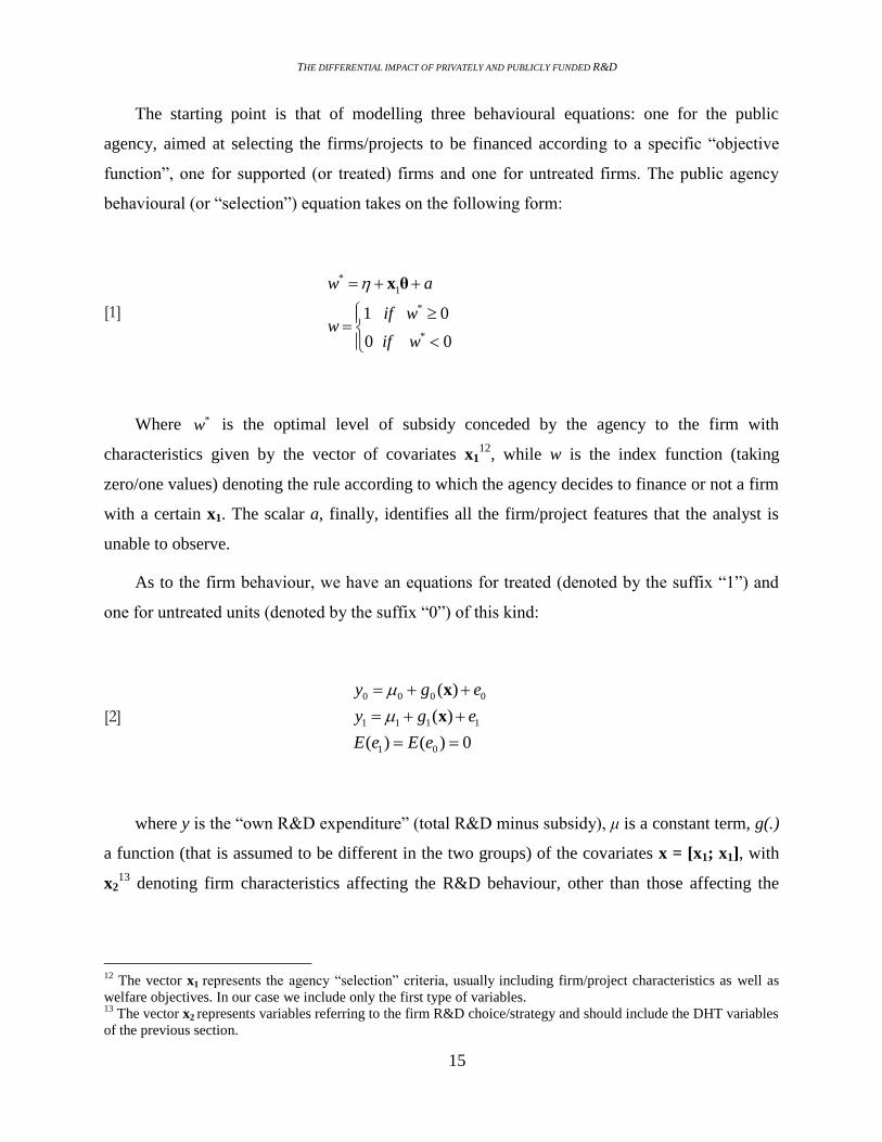
The starting point is that of modelling three behavioural equations: one for the public
agency, aimed at selecting the firms/projects to be financed according to a specific “objective
function”, one for supported (or treated) firms and one for untreated firms. The public agency
behavioural (or “selection”) equation takes on the following form:
[1]
*
1
*
*
1 0
0 0
w a
if ww
if w
x θ
Where *w is the optimal level of subsidy conceded by the agency to the firm with
characteristics given by the vector of covariates x112
, while w is the index function (taking
zero/one values) denoting the rule according to which the agency decides to finance or not a firm
with a certain x1. The scalar a, finally, identifies all the firm/project features that the analyst is
unable to observe.
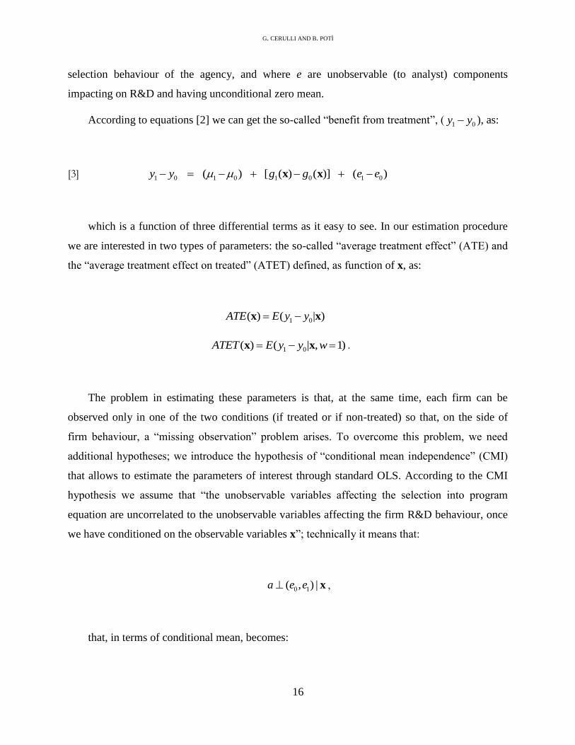
As to the firm behaviour, we have an equations for treated (denoted by the suffix “1”) and
one for untreated units (denoted by the suffix “0”) of this kind:
[2]
0 0 0 0
1 1 1 1
1 0
( )
( )
( ) ( ) 0
y g e
y g e
E e E e
x
x
where y is the “own R&D expenditure” (total R&D minus subsidy), μ is a constant term, g(.)
a function (that is assumed to be different in the two groups) of the covariates x = [x1; x1], with
x213
denoting firm characteristics affecting the R&D behaviour, other than those affecting the
12
The vector x1 represents the agency “selection” criteria, usually including firm/project characteristics as well as
welfare objectives. In our case we include only the first type of variables. 13
The vector x2 represents variables referring to the firm R&D choice/strategy and should include the DHT variables
of the previous section.
G. CERULLI AND B. POTÌ
16
selection behaviour of the agency, and where e are unobservable (to analyst) components
impacting on R&D and having unconditional zero mean.
According to equations [2] we can get the so-called “benefit from treatment”, ( 1 0y y ), as:
[3] 1 0 1 0 1 0 1 0 ( ) [ ( ) ( )] ( )y y g g e e x x
which is a function of three differential terms as it easy to see. In our estimation procedure
we are interested in two types of parameters: the so-called “average treatment effect” (ATE) and
the “average treatment effect on treated” (ATET) defined, as function of x, as:
1 0( ) ( | )ATE E y y x x
1 0( ) ( | , 1)ATET E y y w x x .
The problem in estimating these parameters is that, at the same time, each firm can be
observed only in one of the two conditions (if treated or if non-treated) so that, on the side of
firm behaviour, a “missing observation” problem arises. To overcome this problem, we need
additional hypotheses; we introduce the hypothesis of “conditional mean independence” (CMI)
that allows to estimate the parameters of interest through standard OLS. According to the CMI
hypothesis we assume that “the unobservable variables affecting the selection into program
equation are uncorrelated to the unobservable variables affecting the firm R&D behaviour, once
we have conditioned on the observable variables x”; technically it means that:
0 1( , ) |a e e x ,
that, in terms of conditional mean, becomes:
THE DIFFERENTIAL IMPACT OF PRIVATELY AND PUBLICLY FUNDED R&D
17
0 0( | , ) ( | ) 0E e w E e x x and 1 1( | , ) ( | ) 0E e x E e x x .
It can be shown that, after this hypothesis, the previous parameters become:
1 0 1 0( ) ( ) [ ( ) ( )] ATE g g x x x
1 0 ( 1)( ) ( |w=1) ( )wATET E y y ATE x x .
To get the ATE and ATET (unconditional on x) we only have to average over the support of
x, obtaining:
1 0 1 0( ) [ ( ) ( )]ATE E g g x x x
( 1)[ ( )]wATET E ATE x x .
The final step is the arrive to a sample estimate of those parameters, that, of course, has to be
done in terms of observable variables. To achieve this task we introduce the so-called “switching
regression” as:
1 0(1 )y wy w y
where y is observable. By replacing y1 and y0 with their expression from [2], we get the
following relation:
0 0 1 0 1 0( ) ( ) [ ( ) ( )]y g w w g g u x x x
G. CERULLI AND B. POTÌ
18
where 0 1 0( )u e w e e . Moving toward a parametric form of g by putting: 1 1( )g 1x xβ
and 0 0 0( )g x xβ we can rearrange the previous equation getting, after simple manipulations,
the following “reduced form” regression equation:
[5] ( | , ) [ ]E y w w w 0 xx xβ x μ δ
where it can be proved that 0 0 , = ATE, 1 0δ = (β -β ) and
xμ = E(x) . Equation [5]
can be estimated consistently by OLS, and once obtained the OLS parameters we can get the
various treatment effects by simple transformations of the type:
[6]
1
( 1)
ˆ ˆ
ˆˆ ˆ( ) ( )
ˆˆ ˆ (1/ ) ( )
ˆˆ ˆ( ) ( ) .
NT
i
w
ATE
ATE
ATET N w
ATET
x x x δ
x x δ
x x x δ
Relations [6] are all estimable since they are function of observable (to analyst) components.
The only difficulty is that of obtaining standard errors for the ATET, a problem that can be
overcome by bootstrapping.
As to the form of our “control group” it is important to stress that it is represented by a
group of firm/year that: (1) did not apply for subsidies at all, (2) applied for subsidies but was
refused, i.e., did not receive any public funding commitment for their project application during
the period (2000-2004). Observe in any case that, as projects generally last more than one year, a
given firm getting a project accepted in one year becomes treated also for the next year just
according to its project time span; it means that the number of treated observations (again,
firm/year) increases after our public fund’s spreading procedure, reducing the number of
untreated observations accordingly.
THE DIFFERENTIAL IMPACT OF PRIVATELY AND PUBLICLY FUNDED R&D
19
The firms of the control group are all recorded in the “Anagrafe della ricerca”, in so showing
a certain willingness/propensity to apply for FAR /Law 488 subsidy policy (that is, a certain
homogeneity with treated units). Moreover, in our sample treated and untreated firms have very
similar structural characteristics, except for Size and Knowledge. Nevertheless, since we use a
linear multiple regression we do not need to generate a “similar-to-treated” control group as
required, for instance, by Matching approaches: in our case it is sufficient to insert (in particular)
those covariates controlling for firms differences as we did for the Size and Knowledge in our
application. However, in the output additionality exercise (that on the effect of subsidies on the
number of filed patents), we will make use of a Matching model because more suitable in that
context of analysis.
In what follows we present results by estimating the parameters of [6]. We only want to
stress that in the firms’ subgroup analysis we will work under the additional hypothesis that
1 0( ) ( )g gx x , that makes ATE = ATET simplifying significantly the analysis.
7 Results
According to the model proposed above this section presents the main results on “input
additionality”, that is on the capacity of firms to “top up” an addition R&D expenditure to their
observed R&D performance, net of the subsidy component (i.e. what firm should do in absence
of the subsidy). On average, the additionality occurs when the value of the parameter is
positive and statistically significant. Nevertheless the possibility of estimating ATE(x) as well as
ATET(x) does shed more light on the distributional characteristics of the single parameters ATE
and ATET, in so providing idiosyncratic firm-specific treatment effect; indeed, going beyond an
aggregated average value, seems of a great importance for a more in-depth understanding of the
policy effect under study. The report of results are organized as follows:
- first, we provide results for the pooled regression for detecting, at an aggregated
level, if there exists a “crowding-out” or an “additionality” effect on firm own R&D
G. CERULLI AND B. POTÌ
20
investment. Here we work under the hypothesis that 1 0( ) ( ) ( )g g g x x x , so that the
parameter estimates both the ATE and ATET.
- second, we allow for 1 0( ) ( )g gx x so that =ATE ATET; then we fix our attention
on the estimation of the distribution of ATET(x) showing its graphical representation
and the main characteristics of its distribution. As we said, this is a firm-specific
measure of the causal effect of FAR on firm R&D performance;
- third, we go beyond the aggregate result by splitting our sample according to
different and heterogeneous firm characteristics. In particular we estimate regression
[5] in subsets of firms by size, Italian macro-regions, type of technology and by the
share of the project costs covered by the subsidy; finally, an analysis of the mix of
instrument is also provided: here we are interested in seeing if a different portfolio of
subsidy generate differential effects;
- fourth, we provide evidence upon the differences in term of economic and structural
characteristics between the group of firm performing additionality and those
performing crowding-out. These step is drawn upon the results of the second step.
Here what matters is to identify the leading factors characterizing the policy’s
success and possibly their relations with the agency’s selection criteria.
Input additionality: overall sample
Table 8 considers results from the aggregated sample under the 1 0( ) ( )g gx x hypothesis.
Column 1 shows the effect of the treatment dummy on the own R&D expenditure without
covariates (simple t-test comparison between the two group), while column 2 and 3 introduce
some cleaning of the data.
The most important regression, which we labelled the “fundamental” one, is in column 4,
where a series of covariates has been introduced: it shows a positive and significant average
treatment effect on treated (ATET) of FAR on firm own R&D expenditure of about 801 thousand
THE DIFFERENTIAL IMPACT OF PRIVATELY AND PUBLICLY FUNDED R&D
21
Euros: it means that this additionality (that can be seen as the “own R&D of treated” minus the
“own R&D of untreated” units) is of about 40% of the untreated firms’ R&D average14
.
The Size is also positive and strongly significant, with an increase of about 4 thousand Euros
of own R&D expenditure per one additional employee; also the presence of collaborative project
(Collaboration) marks a positive and highly significant effect (about 9,8 millions of Euros), as
well as the presence of a subsidy allocation from the agency (with a value of 3,3 millions of
Euros). Observe the negative significance of the automatic policy instrument15
(Art. 14, i.e., tax
credit) showing the presence of a strong crowding-out (about -2,3 millions of Euros).
Apart from the Leverage (just very slightly positive and significant) the other financing
variables (Cash-flow and Equity) are not significant, although with a positive sign, in explaining
the firm own R&D performance. Cost variables are not significant too. It seems, in other words,
that the liquidity constraints as well as the ability to find external source of financing are not
distinguishing factors in explaining the additionality’s capacity of the firm. As it will be more
understandable later, this aspect deserves further attention.
Estimation and distributional features of ATE(x) and ATET(x)
According to the estimation of equation [5] and to formulas [6], it is possible to calculate the
firm-specific ATE(x) and ATET(x), with their distributional characteristics. In this section we
are working under the hypothesis that 1 0( ) ( )g gx x .
Figure 1 shows the graphical representation of the ATE(x) and ATET(x) for FAR in the
overall sample, while the descriptive characteristics of the ATET(x) distribution are set out in the
Table 9.
Table 9, as well as figure 1, emphasizes one of the most important results of our research:
the median of the ATET(x) is about zero. It means that half of our sample perform a crowding-
14
More in detail, the average own R&D expenditure of the untreated units is about 570 thousand Euros. Indeed:
(801-570)/570 ≈ 0.40. 15
Since the benefit from “tax credit” is calculated on past R&D activities we have checked the presence of
additionality/crowding-out for this fiscal measure also by allowing for one and two time lags of the own R&D
expenditure, getting in any case the same negative result as in the contemporaneous case of Table 8 (a table on these
last estimates have not been reported).

G. CERULLI AND B. POTÌ
22
out, whereas the second half an additionality result. What is interesting too, is that the ATET(x)
mean is positive (and significant), but only because of the existence of a strong right asymmetry
of the ATET(x) distribution, with positive values significantly higher than negative value in
absolute terms. This is a surprising, as well as a very characterizing aspect of FAR, that only the
knowledge of the entire distribution of the effect can put into evidence. Observe that the mean of
the ATET(x) in table 9 is about 878 thousand Euros, that is slightly different from the value of
801 obtained in table 8: this is due, as we said, to the hypothesis that 1 0( ) ( )g gx x of the
ATET(x) model. Nevertheless this difference is largely negligible and in the rest of the paper we
will work under the assumption that 1 0( ) ( )g gx x .
8 The analysis by subsets of firms
So far we have considered results from an aggregated perspective. Nevertheless firms are in
their essence strongly heterogeneous and we expect to find differences in FAR effect according
to different subgroups of firms. In particular we are interested in shedding some light on the size,
sectoral specialization, geographical origin and degree of financial support for these firms. The
next sections show the results.
Additionality by size
From table 10 it is immediate to see that only for large (and very large) firms there is a
significant positive additionality (about 1.148 and 2.273 thousand Euros respectively). SME’s
effect is neutral (neither crouding-out, nor additionality), while small firms present a negative
sign (-174), even if not significant.
The Size, as in the pooled sample, is always positive and significant, but its magnitude
lowers passing from small to very large firms. Knowledge, as expected, is positive and
significant only for large and very large firms, since they rely more on patenting activity than
SMEs. The dummy “Only Art. 14” (tax credit) is negative and significant for SMEs, while it is
THE DIFFERENTIAL IMPACT OF PRIVATELY AND PUBLICLY FUNDED R&D
23
dropped for large firms (since this automatic instrument refers only to small sized enterprises).
The variable Collaboration (presence of R&D project collaborations) and Objective 1 (depressed
areas) are positive and significant only for large and very large firms. The variable Collaboration
for SMEs is not significant: the estimator has a large range of variation. There are, among other
things, differences between small firms (with a positive sign) and medium firms (with a negative
sign)16
.
The Leverage is (slightly) positive and significant only for medium sized enterprises (50-
100 employees), while the Cash-flow has a negative and significant effect only for large and very
large firms; notice, however the positive and significant (but only at 10%) coefficient of Equity
for large firms: it seems that larger firms prefer to use external rather than internal sources to
finance their R&D projects, while SMEs seem prefer internal sources (indeed, for medium sized
enterprises the Cash-flaw is positive and quite significant).
Additionality by sectoral specialization in manufacturing
Quite surprisingly table 11 shows a positive and significant effect of FAR on manufacturing
low-tech firms (about 868 thousand Euros), although high and medium tech present positive
values too (with a value for high-techs that is twice that of medium-techs). The size of these low-
techs is in any case quite high, about 320 employees, although they are few when compared with
the number of observations of the other types of firms (we are left with only 317 low-techs).
Furthermore, the level of additionality of these low-techs firms is very close to that got by the
full sample. As expected, the variable Knowledge is highly positive and significant for high-tech
manufacturing firms and only positive (but not significant) for medium and low-techs. The Size
continues to be an important factor in explaining own R&D performance for all types of firms,
while tax credit (Only Art. 14) produces a significant crowding-out only for high-techs.
16
Probably the results are due to two factors: first, not all the collaborative projects are included in our dataset
(which is the result of a merging between three different starting datasets), and second the collaborative projects
include top-down programmes in which mainly large firms participate.
G. CERULLI AND B. POTÌ
24
Additionality by Italian macro-regions
Table 12 shows that the effect (always the ATET) is positive and significant in the North
and Center of Italy, with a value of about 735 (North) and 1.600 (Center) thousand Euros
respectively. For the South the ATET is not significant and also negative in its level.
Nevertheless, it seems of worth to observe that the number of observations is not equally
distributed: the North has the greater number of about 3.000 while the South just 242. Observe
again the joint significance of Size, Collaboration, Objective 1 and Subsidy allocation for all
three regressions. Finally, Only Art. 14 remains negative and significant as in the pooled
regression.
Additionality according to different financing intensity
Table 13 shows regression comparison according to three percentile classes of the
“financing intensity” (defined as the subsidy share of the total project cost): w1, w2 and w3 are
treatment dummy variables for low, medium and highly financed firms respectively.
We can observe that, as soon as we move towards more intensively financed firms, the table
sets out that the level of the effect increases: from about 500 thousand Euros of additionality in
the first and second class, to 1.890 in the third one; furthermore, only for the third percentile
class the effect is really significant. This results puts into evidence that the positive effect of the
subsidy starts only above a certain threshold, that in this application is a financing of about 50 %
of the total cost.
9 Impact by instrument and mix of instruments
For the analysis of the effect of single instruments as well as of their mix, we start by
defining a dummy for each instrument:

THE DIFFERENTIAL IMPACT OF PRIVATELY AND PUBLICLY FUNDED R&D
25
D1= bottom-up Law 297 (Art. 5 and 6). They are 1.410 total cases, of which 1.204 alone.
D2= top-down measures (Art. 11 and 12). They are 140 cases, of which 79 alone.
D3 = bottom-up Law 488. They are 413 cases, of which 312 alone.
D4= other instruments.
What do these dummies compare? According to their definition, for each instrument they
compare two groups of firms: the first one is that in which the instrument was used by a firm
with or without other instruments and the second on is that in which the measure17
is not present,
i.e., only other instruments are included or firms receive no subsidy. In this way we obtain the
additionality effect by single instrument, and we can compare the effects among different
measures. Moreover, we tested the additionality effect of different mix of instruments (for
instance: D1 x D2) with their complement.
Table 14 shows these effects for single policy instruments as well as for some of their
combinations. As it is easy to see bottom-up projects (D1 for Law 297 and D3 for Law 488)
provide significant additionality in line with the average value (pooled regression of table 8).
Top-down projects, on the contrary, show a negative and significant effect: nevertheless, this last
result hinges on only 35 observations18
, so it has to be taken with caution.
When bottom-up projects are joint together, their strength increases considerably (see the
coefficient of D1D3). The other results do not deserve further comments, since the number of
observations it too low to draw reliable conclusions.
In order to deepen the analysis on the mix of instruments we also performed single
regressions using a new dummy for each instrument, built in the following way: we compared
two groups of firms, those exploiting the single instruments (without any other measure) and
those using the same instrument joined with other measures. We got results (table not reported)
only for bottom-up instruments (Law 297 and Law 488) because of few observations. We found
that the difference is positive in the case of joined instruments for both measures, but statistically
17
We use the words “instrument” or “measure” interchangeably. 18
The introduction of covariates reduces the number of observations because of the numerous missing values.
G. CERULLI AND B. POTÌ
26
significant only for the Law 488. In particular we got a coefficient of 2.643 thousand Euros with
a p-value of 0,155 for bottom-up measures of Law 297 (with 552 observations) and a coefficient
of 7.447 thousand Euros with a p-value of 0,039 for bottom-up measures of Law 488 (with 167
observations).
10 Structural differences between the “crowding-out” and the “additionality”
group
Which are the distinguishing characteristics of the group of firms performing crowding-out
compared with those performing additionality? Answering this question seems important, both
analytically, because it allows to go beyond the aggregate result on the ATET, and normatively,
since it appears to be an important information for policy makers.
We saw that half of the supported unit do an additionality, while the other half do an
crowding-out result. This means that we can establish a clear-cut threshold, the median of the
ATET distribution, tracing out quite clearly the composite effect of the policy at stake.
Operatively, we form two groups, the “crowding-out” and the “additionality” group,
according to the (zero) median of the ATET(x), and we try to characterize them by comparing a
wide set of variables-characteristics in order to shed more light on which are the essential
(structural) differences among these two groups. We point to answer this question: which factors
make a firm more able to exploit in an additional way the support received?
The literature suggests to look at three groups of variables, according to three theoretical
perspectives we take into account: “industrial organization”, “corporate financing” and
“innovative capacity” variables. Results on these three set of variables are visible in table 15.A
and table 15.B.
By looking at the mean and, more correctly (since many variables are strongly asymmetric
with a long right tail) at the median of the distribution of these variables, we can observe some
important aspects:
THE DIFFERENTIAL IMPACT OF PRIVATELY AND PUBLICLY FUNDED R&D
27
The Size, in terms of number of employees, is an harsh demarcation factor: the group of
firms performing additionality is, on average, more than 10 times larger than the group of firm
doing crowding-out. In terms of median, since we deal with very large right tails, this value
becomes about 6 times, a still high value.
In terms of Turnover, both the mean and median of the additionality group is largely higher
than that of the crowding-out group. It confirms the result on Size, with the additionality group
performing a median turnover about 10 times greater than that of the crowding-out group.
What is surprising is that, in terms of R&D per employee, i.e. in terms of “firm input
capacity” (or R&D competence) in an innovation function, the two groups reach a very similar
result: quite unexpectedly, the “crowding-out” group performs in median 6.5 thousand Euros of
R&D per employee compared with a value of 5.2 of the additionality group. R&D intensity
capacity doesn’t seem hence an essential factor for explaining the ability of performing
additional R&D expenditure, once received a proper support19
.
For the sake of brevity, by looking at all the corporate financing variables (Cash-flow,
Leverage, Equity, etc.) we can observe a general similarity in the two group. It seems that, from a
financial point of view they are quite indistinguishable, so that no differential financial constrains
are able to justify different additionality performance (we only observe a little higher level of
Cash-flow availability in the additionality group).
The Operating profit margin (OPM, a proxy of the firm relative market power) does not
seem to matter as well. We cannot invoke, at least at this stage, the idea that the additionality
group includes firms with a greater market power compared to the “crowding-out” group.
The share of R&D project costs covered by FAR support is the same in the two group
showing that also this element does not participate in explaining potentially differential
advantages of one group over the other.
Also in terms of Sector the two groups do not present appreciable differences: in the
crowding-out group the first two sectors (in terms of number of observations) are the machinery
industry (22%) and chemicals/pharmaceuticals (12%), as well as in the additionality group where
the machinery industry is the first one (18%) followed by chemicals/pharmaceuticals (15%).
19
Of course, since we are looking at firms generally having an R&D activity, the lower the firms size (as in the case
of the “crowding-out” group) the higher their R&D intensity.
G. CERULLI AND B. POTÌ
28
The Region too does not mark differences: Lombardia, Emilia Romagna, Veneto and
Piemonte are the main regions in which firms are located and follow in the same order in both
the samples.
Finally, as to the “delay between the project application and final positive acceptance” no
differences arise: both samples present an average of about 22 months and the form of the
distribution of this variables is also very similar in the two groups.
The most important difference, apart from the size, refers to the “propensity to patent”. The
average number of patents applications of the additionality group is about 6 times that of the
crowding-out group (and 3 times in terms of median). The median investment rate of the
additionality group is not particularly different from that of the crowding-out group and is in
both cases negative.
What can we conclude from this analysis? Very concisely, we can state that financial
constraints do not seems able to qualify a different “propensity” to perform additionality. Indeed,
while financial variables affect the public agency selection, they do not appear able to
disentangle differences within the group of treated units (either if they do additionality or
crowding-out). This is a first important point.
The size is an essential demarcation factor. Larger firms tend to perform additionality more
easily than smaller firms and this aspect deserves further inspection.
A central point is that, while the two groups present a similar R&D intensity, they have very
different performances in terms of patenting activity. This requires some further discussion. In
fact, what seems to emerge is a greater ability of the “additionality” group in transforming their
inventive inputs (mainly, the R&D intensity) in innovative outputs (in our case, the number of
patent applications): this identifies a different “innovation production function” in the two
groups. This clearly can rely on two essential ingredients: “scale economies” (linked essentially
to the firm size) and “strategies” (firm choices and objectives). As to the first element a well
known literature (starting from the Schumpeter Mark II paradigm of the innovation process)
points out the benefits (increasing return to scale) deriving from a higher size: wider and better
internal division of labour (benefits from specialization), greater capacity of
internalizing/exploiting network and knowledge (R&D linked) spillovers, greater facility to
reach and contact new markets, greater market and non-market (political) power, and so on. As
THE DIFFERENTIAL IMPACT OF PRIVATELY AND PUBLICLY FUNDED R&D
29
to the second element (“strategies”), it seems possible to observe a greater propensity to grow up
in the additionality group rather than in the crowding-out one. It could be quite puzzling since
the second group starts from a very lower size. Probably this mirrors the specific Italian system
of innovation, where SMEs (the great majority of firms) seem to be historically more projected
towards short-term returns (profits) than long-term objectives, such as the growth. Many
previous researchers, indeed, have emphasized how Italian SMEs are reluctant to strategies
pointed at enlarging the scale of production (through, for example, an active financing on stock
markets), in so remaining, essentially, under-capitalized. This is due, among other things, to the
Italian traditional familiar ownership of the firm and on its connected “fear” to lose power and
strategic control.
In conclusion, a different innovation function (stimulated by a different average size) and
the scope of the strategies pursued, seems to affect the occurring of a crowding-out rather than an
additionality behaviour more than the industrial structure (market power), corporate financing
components (leverage, equity, cash-flow), or a strict knowledge input capacity (R&D intensity).
11 The analysis of the “output additionality”: the effect of firm additionality
on patents
The forgone analysis focused on the “input additionality”, i.e. on measuring the effect of
FAR on the target variable, the firm “own R&D expenditure”. If the main objective of FAR is
that of enlarging the R&D performance of Italian firms, own R&D is the proper variable to look
at.
Nevertheless, as suggested by many authors, the enlargement of firms’ R&D expenditure
should be seen only as an intermediary step. Indeed, the public agency, in implementing its
technological policy, should be interested in enhancing the firms’ innovativeness, where an
increase in R&D is an essential precondition. In the innovation production function, indeed, the
R&D activity is the main ingredient (the “input”), but nothing assures that an increase in R&D
will be automatically translated into an increase in the firm innovative performance; neither in
the third and final step of this chain, the firm economic profitability deriving to the innovation
G. CERULLI AND B. POTÌ
30
performance. Figure 2 tries to enlighten this chain: FAR policy is on the upstream point of the
link between R&D and economic performance, that is the downstream point. In each of these
three steps different elements participate in strengthening or weakening the links.
In this section we pay attention to the second link of figure 2, regarding the effect of FAR on
firms’ innovativeness, measured in terms of “number of filed patents”, via the effect of FAR on
R&D performance. This last sentence deserves further explanation. Indeed, it seems incorrect to
study in a “direct” manner the effect of a an R&D policy on technological output (patents, for
example), without in other words passing through the pre-existing effect on R&D. More
precisely, adopting a “two steps” approach (from policy to R&D, from R&D to innovation)
seems to be a more reliable procedure than a “one step” method (from policy to innovativeness).
Many authors adopted the one step pattern, but we prefer the two steps, since what we need, in
order to judge the effectiveness of a policy on innovativeness, is its ability in fostering
innovation via its capacity in fostering R&D additionality. In other words, we are interested in
measuring the effect of the “additionality” brought about by FAR on firm innovativeness, or, put
differently, the effect of the incremental R&D activated by FAR on patents. At this stage,
however, we do not go into the direction of analyzing the third and final step (from
innovativeness to economic performance).
Operatively, we have to translate this reasoning into a model able to catch the link between
FAR and R&D additionality, and that between R&D additionality and innovativeness. The idea
is to apply the following procedure, based on the “Matching approach”:
Step 1.
By a Nearest Neighbour Matching (NNM) obtain the “own R&D expenditure” of the firm i-
th’s non-supported nearest neighbour. Accordingly, take this value as “the level of R&D the firm
would have done without any public intervention”.
THE DIFFERENTIAL IMPACT OF PRIVATELY AND PUBLICLY FUNDED R&D
31
Step 2.
Split the “total R&D expenditure” of the firm i into its three components: (1) the NN-own
R&D of step 1, (2) the level of the subsidy received by the firm i, (3) the level of the
idiosyncratic “additionality” performed by the firm i.
Step 3.
Calculate a Poisson regression of the “number of patents” on those three components plus
covariates, “only” on the sample of supported firms. If the “additionality” component generate
positive and significant results we can conclude that an effect of FAR on innovativeness does
exist.
According to the Step 1, we implement the NNM whose results on the goodness of the
performed matching can be seen in figure 3. Here we can observe that the distribution of the
“propensity scores” after the NNM in the supported and non-supported firms are very similar
compared to the pre-matching situation in which they appeared very dissimilar: it indicates that
the we can trust our matching approach.
After Step 1 and according to Step 2, then, we can calculate the “own R&D expenditure” of
the firm i-th’s non-supported nearest neighbour that we indicate as ( )NN i C
jR , as well the level of
additionality for the firm i, i , obtained as the difference between the own R&D of firm i and
( )NN i C
jR . We finally indicate with iS the level of the subsisy obtained by the firm i-th.
Finally, we implement Step 3 by splitting (only for the supported firms, of course) the “total
R&D expenditure” (Ri) into its three “potential components” (( ) , , NN i C
j i iR S ), applying a
standard Poisson regression of the type:
( )( , , , )NN i C
i j i iPAT f R S x

G. CERULLI AND B. POTÌ
32
where PATi is the number of patents filed by the firm i and x a set of covariates20
. As we
said, we are particularly interested on the effect of αi .
Table 16 shows the results of this Poisson regression. The estimation of the parameters are
semi-elasticities. As it is immediate to notice, the variable Additionality ( i ) is significant and
positive with a value of 0,035: it means that, on average, if the additionality increases of 1
million of Euros (this is our scale), then the patenting activity increase of 3,5%. This value for
medium and low tech firms reach a level of about 8% and 30% respectively. Privately financed
R&D is significant and positive only for low-techs (with a semi-elasticity of 0,27) and the level
of the subsidy only for medium (with a level of 1,7).
This result strengthens the conclusion we have reached on input additionality (own R&D
investment): also on the side of the capacity of activating firm innovativeness FAR seems to
have been effective. This is the conclusion reached by our “two steps” procedure. Nevertheless,
the reduced number of observations do not allow us to look inside this aggregated result (as we
did in the case of input additionality). A result, however, deserves more attention: both in terms
of increased R&D expenditure and in terms of growth in the number of filed patents, FAR seems
to have been particularly successful for low-tech firms. They are, however, low-techs of large
size probably trying to perform a technological shift from more traditional to more sophisticated
products and process although belonging to very traditional sectors; at the same time they can be
probably seen as the “high-tech of the low-tech”, that is, those firms working on the
technological frontier of their sectors. In any case, the idea that FAR has been able to increase
the technological underpinnings of these kind of firms seem to be an additional proof of its
success in terms of ability to promote innovation exactly where new technologies are generally
less widespread.
20 Since the NNM already makes use of the covariates used in the regression analysis, in the Poisson regression we only use as covariates: Region, Sector, Time and Size.

THE DIFFERENTIAL IMPACT OF PRIVATELY AND PUBLICLY FUNDED R&D
33
12 Some results on firm economic performance
Our last analysis points to measure the impact of Far on some economic performance
indicators. We consider the following three indicators: the labour productivity (measured simply
as the ratio of the turnover to the number of employees), the profitability (as operating profit
margin) and growth (as turnover’s rate of growth). We calculate these indicators in the
crowding-out and additionality group along the period examined by this exercise (2000-2004).
This is not a post-treatment analysis, as we do not have information on accounting variables after
2004, but we believe it to be anyway a useful exercise to describe the temporal pattern of the Far
effect.
Figure 4 sets out the results. It is easy to observe that productivity and profitability follow a
very similar path. Indeed, the additionality group gets: a better performance in the first two years
(2000 and 2001), a result very similar to the crowding-out group in 2002, a disadvantage in
2003, and again an outcome similar to the crowding-out in 2004. Overall, the figure seems to
show quite clearly a lack of a uniform “dominance” of the additionality group. Indeed, what
seems to emerge is that its starting advantage in 2000 reduces during the period considered until
no difference in the two groups arises. How can we account for this puzzling pattern? Along with
this econometric analysis, the FIRB project has also realized a survey on 3400 firms receiving at
least one public R&D and innovation support in 1998-2007. The results from this survey -
conducted by the Confidustria (the Italian association of entrepreneurs) - can help to explain
quite well the previous pattern. In fact, what emerges from this survey is that the 93% of firms
cover their R&D project’s costs by self-financing, more than 60% use public funds and only 25%
exclusively self-financing. Nevertheless, problems coming from time delays in funds’ provision
and from uncertainty in the actual availability of public money, generate (further) firm financial
constraints. Indeed, firms end up by use self-financing to cover in advance accepted project’s
costs and more than 70% of them declare to suffer of heavy liquidity problems because of that.
This phenomenon is particularly constraining for firms deciding to add incremental projects to
those allowed by the public incentive (that is, for companies doing additionality). In this sense
the pattern of productivity and profitability is legible according to this perspective. Of course, as
our dataset is unable to see after 2004, inferring about the post-treatment long-run effects of the

G. CERULLI AND B. POTÌ
34
subsidy is not possible. In this sense, we cannot explore if a recovery of the additionality group
will occur, once the beneficial market returns from the additional innovative projects will appear.
In terms of economic growth, finally, the median shows no particular differences in the two
groups, although the results on the mean seem to set out a better performance of the crowding-
out group. Given the high skewness of this variable, however, we prefer to rely on results on the
median rather than on those on the mean.
13 Conclusion
According to the results provided by our model, FAR seems to have been successful both in
terms of its capacity to promote “input additionality” (own R&D performance) and “output
additionality” (patenting performance): we got a 40% of R&D additionality for the average firm
(about 800 thousand Euros of additional “own R&D investment”), and a 3.5% increase in the
number of patents for any 1 million of “additional” firm own R&D expenditure.
Nevertheless substantial differences concern various subsets of firms. As to the two groups
of firms performing additionality and doing crowding-out, we observe that firms doing
additionality are generally larger, more oriented to patent, more prompt to enlarge their fixed
capital stock, but similar to the crowding-out group for R&D intensity, structure of costs and
corporate financing variables. How can we explain this findings? In the paper we embrace an
explanation based on the role played by “scale economies” on one hand and “strategies” on the
other:
- larger firms exploit higher “scale economies” through greater internal division of
labour (specialization), access to wider internal and external networks, ability in
generating and absorbing spillovers, market/political power, easier access to credit
and equity etc.;
- different “strategies” seem to be at work, as larger firm appear more “forward
looking” at long-term objective. Italian SMEs, on the contrary, seem to be

THE DIFFERENTIAL IMPACT OF PRIVATELY AND PUBLICLY FUNDED R&D
35
historically more projected towards short-term returns (immediate profits). This is
due, among other things, to the Italian traditional “familiar ownership” of the firm
and on its connected “fear” to lose power and strategic control.
Having found such features of the “additionality” group pushes us to rethinking about
the selection criteria adopted by the agency in order to make policy interventions more
profitable in the field of R&D and innovation. Indeed, finding that corporate financing
variables as well as the structure of costs (in other words, the idiosyncratic firm financial
risk) do not account for performing additionality or crowding-out, should not be surprising:
these are the basic criteria the agency actually uses for selecting “good” firms/projects and
indeed both the two groups were successful in being selected for funding. What makes the
difference relies on other aspects that are more tied to firm behaviours/choices/objectives, as
well as to their size of course.
To be more successful the R&D policies should pay more attention to these aspects. For
a given level of size, the message seems to state that: “strategies” really matter. Doing R&D
without long-run plans in terms of growth, networking, alliances and/or mergers in an even
more competitive and the globalized market seems to be a non-sustainable strategy. The
public agency’s selection procedure should incorporate this message by providing additional
requirements other than the classical balance sheet indicators and project quality: these
requirements are, of course, less tangible than the traditional ones, since they are embedded
in the firm “vision” of itself, of the environment it operates in (competitors, imitators,
innovation leaders), of the evolution of markets and technologies. All issues that are
sometimes culturally determined and conditioned by socio-political mechanisms, as well as
by the economic/territorial atmosphere (more based on competition than cooperation, for
example) the firm is grounded in. Some of the strategic orientation can be found in the firm
medium term plan and the reform of FAR has gone in the right direction, when it has
included two new pre-conditions for the selection of large projects: firms have to demonstrate
the additionality character of the demanded subsidy and have to include a three year R&D
plan.
In sum, FAR seems an instrument more suitable for large firms: in this case it can
operate with largely positive results, while SMEs need more specific and probably targeted
G. CERULLI AND B. POTÌ
36
(not bottom-up) instruments. Large firms are also the natural candidates for top-down
programmes, but at the present state of knowledge it is difficult to say if a satisfactory
additionality results also from that type of policy intervention.
Beyond input and output additionality, of course, other type of effects need to be
checked, concerning changes in firm behaviour, such as anticipation of future projects or
change in the content of projects, as well as change in the R&D localization, but this analysis
can be better developed through surveys.
THE DIFFERENTIAL IMPACT OF PRIVATELY AND PUBLICLY FUNDED R&D
37
References
Aerts K. and D. Czarnitzki (2004), Using Innovation Survey Data to Evaluate R&D Policy: The
Case of Belgium, ZEW Discussion Papers, No. 04-55.
Almus M. and Czarnitzki D. (2003), The effects of public R&D subsidies on firms’ innovation
activities: The case of Eastern Germany, Journal of Business and Economic Statistics, 21,
226-236.
Amemiya T. (1985), Advanced Econometrics, Basil Blackwell.
Arrow K. (1962), Economic welfare and the allocation of resources for invention, in R. Nelson
(ed.), The rate and direction of economic activity, New York, Princeton University Press.
Becker S. and Ichino A. (2002), Estimation of Average Treatment Effects Based on Propensity
Scores, The Stata Journal, 2(4), 358-377.
Bérubé C. and Mohnen P. (2007), Are Firms That Received R&D Subsidies More Innovative?,
UNU-MERIT Working Paper Series, No. 015.
Busom I. (2000), An empirical Evaluation of the Effects of R&D Subsidies, Economics of
Innovation and New Technology, 9(2), 111–148.
Cameron A.C. and P.K. Trivedi (2005), Microeconometrics: Methods and Applications,
Cambridge University Press.
Cerulli G. (2009), Modelling and measuring the effect of public subsidies on business R&D: a
critical review of the econometric literature, Economic Record, forthcoming.
Cerulli G. and Potì B. (2008), Evaluating the Effect of Public Subsidies on Firm R&D Activity:
An Application to Italy Using the Community Innovation Survey”, Ceris-CNR Working
Paper, N. 09/08.
Cohen W.M. and Levinthal D.A. (1989), Innovation and learning: the two faces of R&D,
Economic Journal, 99, 569-96.
Czarnitzki D. and Hussinger K. (2004), The Link between R&D Subsidies, R&D Spending and
Technological Performance, ZEW - Centre for European Economic Research, Discussion
Paper No. 04-056.
D'Aspremont C. and Jacquemin A. (1988), Cooperative and Noncooperative R & D in Duopoly
with Spillovers. The American Economic Review, 78(5), 1133-1137.
Dasgupta P. (1988), Patents, Priority and Imitation or, the Economics of Races and Waiting
Games. The Economic Journal, 98(389):66-80.
Dasgupta P. and Stiglitz J. (1980), Industrial Structure and the Nature of Innovative
Activity. The Economic Journal, 90(358), 266-293.
David P.A. and B.H. Hall (2000), Heart of darkness: modeling public–private funding
interactions inside the R&D black box, Research Policy, 29, 1165-1183.
David P.A., B.H. Hall and A.A. Toole (2000), Is public R&D a complement or substitute for
private R&D? A review of the econometric evidence, Research Policy, 29, 497–529.
G. CERULLI AND B. POTÌ
38
Dehejia R.H. and Wahba S. (2002), Propensity Score-Matching Methods For Nonexperimental
Causal Studies, The Review of Economics and Statistics, 84(1), 151-161.
Duguet E. (2003), Are R&D Subsidies a Substitute or a Complement to Privately Funded R&D?
Evidence from France using Propensity Score Methods for Non-Experimental Data,
University of Paris I Cahier de la MSE EUREQua, Working Paper, No. 2003.75.
González X., Jaumandreu J. and Pazo C. (2005), Barriers to Innovation and Subsidy
Effectiveness, RAND Journal of Economics, 36(4), 930-949.
Greene W.H. (2003), Econometric Analysis, Prentice Hall, New Jersey.
Hall B.H. (2002), The Financing of Research and Development, Oxford Review of
Economic Policy Volume 18, N. 1, 35-51.
Heckman J.J. (1978), Dummy endogenous variables in a simultaneous equation system,
Econometrica, 46(4), 931-59.
Heckman J.J. (1979), Sample selection bias as a specification error, Econometrica, 47, 153-161.
Heckman J.J. (2001), Micro Data, Heterogeneity, and the Evaluation of Public Policy: Nobel
Lecture, Journal of Political Economy, 109(4), 673-748.
Heckman J.J., Urzua S. and E. Vytlacil (2006), Understanding Instrumental Variables in Models
with Essential Heterogeneity, The Review of Economics and Statistics, 88(3), 389-432.
Hussinger K. (2003), R&D and Subsidies at the Firm Level: An Application of Parametric and
Semi-Parametric Two-Step Selection Models, ZEW Discussion Paper, No. 03-63
(forthcoming in Journal of Applied Econometrics).
Ichino A. (2006), The Problem of Causality in the Analysis of Educational Choices and Labor
Market Outcomes, Slides for Lectures, European University Institute and CEPR.
IPTS-Institute for Perspective Technological Studies (2002), RTD Evaluation Toolbox. Assessing
the Socio-Economic Impact of RTD-Policies, IPTS Technical report Series, August.
Kaiser U. (2004), Private R&D and Public R&D subsidies: Microeconometric Evidence from
Denmark, CEBR Discussion papers, No. 2004-19.
Klette T. and Møen J. (1998), R&D investment responses to R&D subsidies: a theoretical
analysis and a microeconometric study, Mimeo, Presented at the NBER Summer Institute.
Klette T.J., J. Møen und Z. Griliches (2000), Do Subsidies to Commercial R&D Reduce Market
Failures? Microeconometric Evaluation Studies, Research Policy, 29, 471–495.
Lach S. (2000), Do R&D Subsidies Stimulate or Displace Private R&D? Evidence from Israel,
NBER Working Papers, No. 7943, Cambridge, MA.
Lechner M. (2001), Identification and estimation of causal effets of multiple treatment under the
conditional independance asumption. In Lechner M. and F. Pfeiffer (eds), Econometric
Evaluation of Labour Market Policies, Physica-Verlag.
Lee M.J. (2005), Micro-Econometrics for Policy, Program, and Treatment Effects, Oxford
University Press.
Lichtenberg F.R. (1984), The relationship between federal contract R&D and company R&D.
American Economic Review Papers and Proceedings, 74, 73–78.
THE DIFFERENTIAL IMPACT OF PRIVATELY AND PUBLICLY FUNDED R&D
39
Lichtenberg F.R. (1987), The effect of government funding on private industrial research and
development: a re-assessment, The Journal of Industrial Economics, 36, 97–104.
Lichtenberg F.R. (1988), The private R&D investment response to federal design and technical
competitions, American Economic Review, 78, 550–559.
Lööf H. and A. Heshmati (2007), The Impact of Public Funds on Private R&D Investment: New
Evidence from a Firm Level innovation Study, in Heshmati A., Y-B. Sohn and Y-R. Kim
(eds), Commercialization and Transfer of Technology: Major Country Case Studies, Nova
Science Publishers.
Maddala G. S. (1983), Limited dependent and qualitative variables in econometrics, Cambridge
University Press.
Malerba F. (1993), The National System of Innovation: Italy, in Nelson R. (ed.), National
Innovation Systems. A comparative Analysis, Oxford Univ. Press, Oxford.
Martin S. and Scott J.T. (2000), The nature of innovation market failure and the design of public
support for private innovation, Research Policy, 29, 437-447.
Metcalfe S. (1995), The Economic Foundations of Technology Policy: Equilibrium and
Evolutionary perspectives, in Stoneman P. (ed.), Handbook of the Economics of Innovation
and Technological Change, Blackwell Publishers, Oxford, 409-512.
Mowery D. (1995), The Practice of Technological Policy, in Stoneman P. (ed.), Handbook of the
Economics of Innovation and Technological Change, Blackwell Publishers, Oxford, 513-
557.
Myers S.C. and N.J. Majluf (1984), Corporate Financing and Investment Decision When Firms
Have Information That Investors Do Not Have, Journal of Financial Economics, 13 (2),
187-221.
Nadiri M.I. (1993), Innovations and technological spillovers, NBER Working Paper, No. 4423.
Pavitt K. (1984), Sectoral patterns of technological change: towards a taxonomy and a theory,
Research Policy, 13, 343–373.
Romer P.M. (1986), Increasing Returns and Long-run Growth, Journal of Political Economy,
94(5), 1002-37.
Romer P.M. (1990), Endogenous Technological Change, Journal of Political Economy, 98(5),
71-102.
Rosenbaum P. and D. Rubin (1983), The Central Role of the Propensity Score in Observational
Studies for Causal Effects, Biometrika, 70, 41–55.
Rubin D.B. (1977), Assignment to Treatment Group on the Basis of a Covariate, Journal of
Educational Statistics, 2, 1-26.
Streicher G. (2007), Additionality of FFD funding. Final report, InTeReg Working paper, No.
49.
Wallsten S.J. (2000), The Effects of Government–Industry R&D Programs on Private R&D: The
Case of the Small Business Innovation Research Program, The RAND Journal of
Economics, 31(1), 82-100.

G. CERULLI AND B. POTÌ
40
Wooldridge J.M. (2002), Econometric Analysis of cross section and panel data, MIT Press.
Zhao Z. (2004), Using Matching to Estimate Treatment Effects: Data Requirements, Matching
Metrics, and Monte Carlo Evidence, Review of Economics and Statistics, 86(1), 91-107.

THE DIFFERENTIAL IMPACT OF PRIVATELY AND PUBLICLY FUNDED R&D
41
TABLE 1. Main features of the "panel_firb" dataset. Note: with the term “subsidy” we intend the level of the public financing according to the “gross grant equivalent” method.
Name Panel_firb
Unit of observation Firm per year
Time span 2000-2004
N. of years 5
N. of firms 2321
N. of observations 11605
N. of supported firms 1845 (1200)
N. of non-supported firms 9760 (10405)
Average firm size 386 employees
Method for the calculus of the subsidy GGE (Gross Grant Equivalent )
Average financing share on costs’ project 0.49
Average project duration 2.7 years
N. of obs. with only one project in the period 56%
Firms located in the North of Italy 65%
A. Average R&D expenditure per year 4,95 million of Euros
B. Median R&D expenditure per year 491 thousand Euros
C. Maximum R&D expenditure per year 467 millions of Euros
D. Average subsidy per year 624 thousand Euros
E. Median subsidy per year 234 thousand Euros
F. Maximum subsidy per year 38,2 millions of Euros
D/A in percentage (mean) 12.5 %
E/B in percentage (median) 49.4 %
F/C in percentage (maximum) 8.1 %
Average Turnover 40.7 billions of Euros
Median Turnover 16 million of Euros
Median R&D intensity 3.06 %
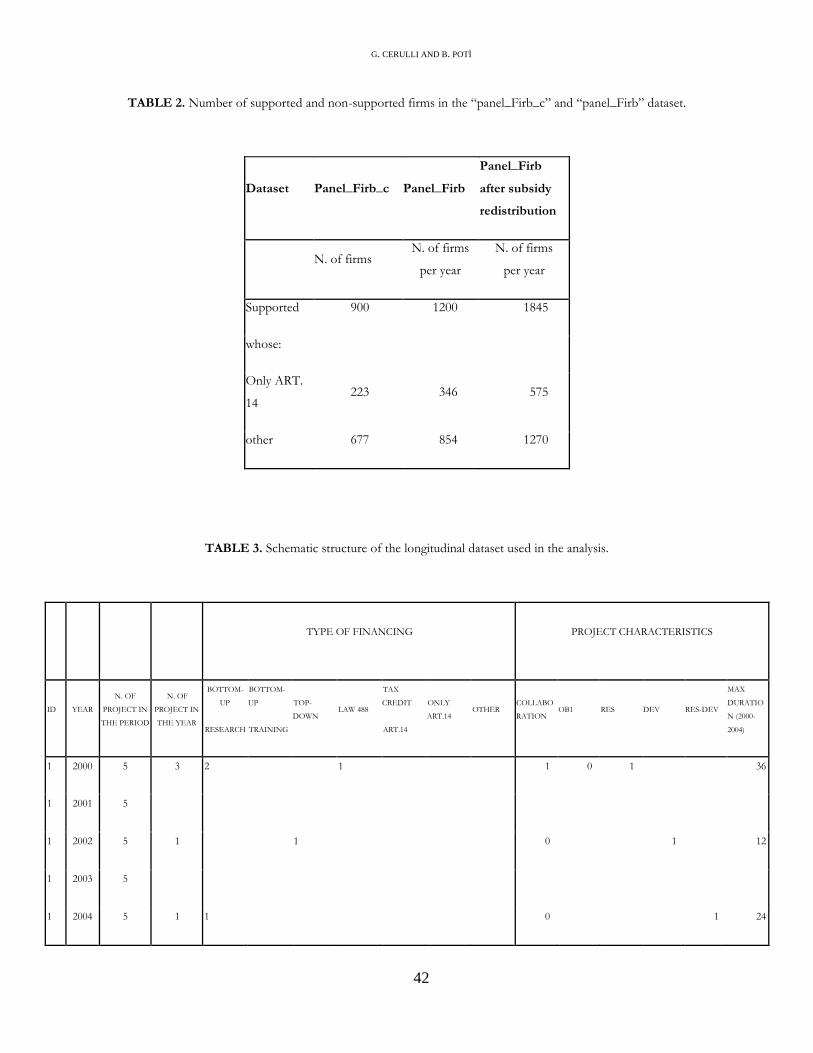
G. CERULLI AND B. POTÌ
42
TABLE 2. Number of supported and non-supported firms in the “panel_Firb_c” and “panel_Firb” dataset.
Dataset Panel_Firb_c Panel_Firb
Panel_Firb
after subsidy
redistribution
N. of firms N. of firms
per year
N. of firms
per year
Supported 900 1200 1845
whose:
Only ART.
14 223 346 575
other 677 854 1270
TABLE 3. Schematic structure of the longitudinal dataset used in the analysis.
TYPE OF FINANCING PROJECT CHARACTERISTICS
ID YEAR
N. OF
PROJECT IN
THE PERIOD
N. OF
PROJECT IN
THE YEAR
BOTTOM-
UP
RESEARCH
BOTTOM-
UP
TRAINING
TOP-
DOWN LAW 488
TAX
CREDIT
ART.14
ONLY
ART.14 OTHER
COLLABO
RATION OB1 RES DEV RES-DEV
MAX
DURATIO
N (2000-
2004)
1 2000 5 3 2 1 1 0 1 36
1 2001 5
1 2002 5 1 1 0 1 12
1 2003 5
1 2004 5 1 1 0 1 24

THE DIFFERENTIAL IMPACT OF PRIVATELY AND PUBLICLY FUNDED R&D
43
TABLE 4. Weight of single instruments in the “panel_Firb” dataset.
Instrument Freq. %
Only ART.14 346 28.83
At least one bottom-up research project 649 54.08
At least one bottom-up training project 13 1.08
At least Law 488 project 166 13.83
At least one top-down research project 47 3.92
At least one Art.14 research project 83 6.92
At least one “other” research project 13 1.08
At least one collaborative research project 153 12.75
At least one OB1 research project 229 19.08
Research and Development Freq. %
Research 199 25.42
Research and development 475 60.66
Development 109 13.92
Total 783 100
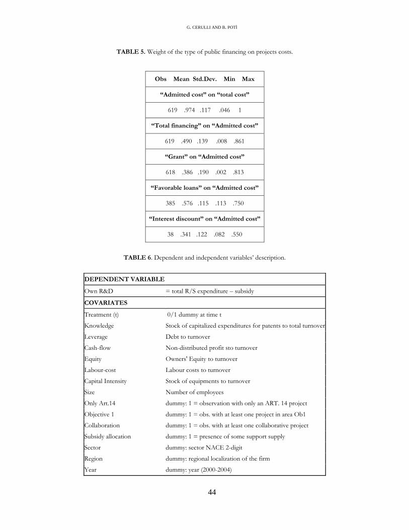
G. CERULLI AND B. POTÌ
44
TABLE 5. Weight of the type of public financing on projects costs.
Obs Mean Std.Dev. Min Max
“Admitted cost” on “total cost”
619 .974 .117 .046 1
“Total financing” on “Admitted cost”
619 .490 .139 .008 .861
“Grant” on “Admitted cost”
618 .386 .190 .002 .813
“Favorable loans” on “Admitted cost”
385 .576 .115 .113 .750
“Interest discount” on “Admitted cost”
38 .341 .122 .082 .550
TABLE 6. Dependent and independent variables’ description.
DEPENDENT VARIABLE
Own R&D = total R/S expenditure – subsidy
COVARIATES
Treatment (t) 0/1 dummy at time t
Knowledge Stock of capitalized expenditures for patents to total turnover
Leverage Debt to turnover
Cash-flow Non-distributed profit sto turnover
Equity Owners' Equity to turnover
Labour-cost Labour costs to turnover
Capital Intensity Stock of equipments to turnover
Size Number of employees
Only Art.14 dummy: 1 = observation with only an ART. 14 project
Objective 1 dummy: 1 = obs. with at least one project in area Ob1
Collaboration dummy: 1 = obs. with at least one collaborative project
Subsidy allocation dummy: 1 = presence of some support supply
Sector dummy: sector NACE 2-digit
Region dummy: regional localization of the firm
Year dummy: year (2000-2004)
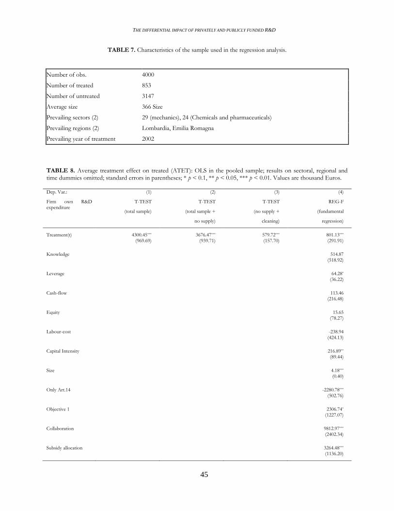
THE DIFFERENTIAL IMPACT OF PRIVATELY AND PUBLICLY FUNDED R&D
45
TABLE 7. Characteristics of the sample used in the regression analysis.
Number of obs. 4000
Number of treated 853
Number of untreated 3147
Average size 366 Size
Prevailing sectors (2) 29 (mechanics), 24 (Chemicals and pharmaceuticals)
Prevailing regions (2) Lombardia, Emilia Romagna
Prevailing year of treatment 2002
TABLE 8. Average treatment effect on treated (ATET): OLS in the pooled sample; results on sectoral, regional and time dummies omitted; standard errors in parentheses; * p < 0.1, ** p < 0.05, *** p < 0.01. Values are thousand Euros.
Dep. Var.: (1) (2) (3) (4)
Firm own R&D expenditure
T-TEST
(total sample)
T-TEST
(total sample +
no supply)
T-TEST
(no supply +
cleaning)
REG-F
(fundamental
regression)
Treatment(t) 4300.45*** 3676.47*** 579.72*** 801.13*** (969.69) (939.71) (157.70) (291.91)
Knowledge 514.87 (518.92)
Leverage 64.28* (36.22)
Cash-flow 113.46 (216.48)
Equity 15.65 (78.27)
Labour-cost -238.94 (424.13)
Capital Intensity 216.89** (89.44)
Size 4.18*** (0.40)
Only Art.14 -2280.78*** (502.76)
Objective 1 2306.74* (1227.07)
Collaboration 9812.97*** (2402.34)
Subsidy allocation 3264.48*** (1136.20)
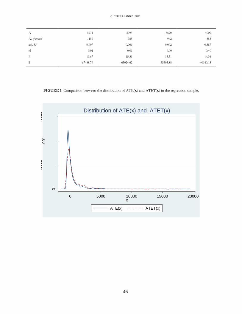
G. CERULLI AND B. POTÌ
46
N 5971 5793 5690 4000
N. of treated
adj. R2
1159
0.007
985
0.006
942
0.002
853
0.387
r2 0.01 0.01 0.00 0.40
F 19.67 15.31 13.51 14.36
ll -67488.79 -65024.62 -55505.88 -40140.13
FIGURE 1. Comparison between the distribution of ATE(x) and ATET(x) in the regression sample.
0
.000
5.0
01
.001
5
Kern
el d
en
sity
0 5000 10000 15000 20000x
ATE(x) ATET(x)
Distribution of ATE(x) and ATET(x)
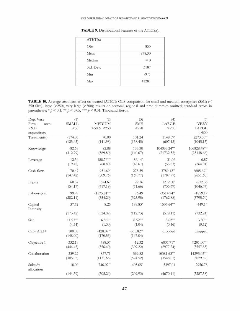
THE DIFFERENTIAL IMPACT OF PRIVATELY AND PUBLICLY FUNDED R&D
47
TABLE 9. Distributional features of the ATET(x).
ATET(x)
Obs 853
Mean 878.30
Median ≈ 0
Std. Dev. 3187
Min -971
Max 41281
TABLE 10. Average treatment effect on treated (ATET): OLS comparison for small and medium enterprises (SMI) (< 250 Size), large (>250), very large (>500); results on sectoral, regional and time dummies omitted; standard errors in parentheses; * p < 0.1, ** p < 0.05, *** p < 0.01. Thousand Euros.
Dep. Var.: (1) (2) (3) (4) (5) Firm own R&D expenditure
SMALL <50
MEDIUM >50 & <250
SME <250
LARGE >250
VERY LARGE
>500
Treatment(t) -174.05 70.00 101.24 1148.59* 2273.50** (125.45) (141.98) (138.45) (607.15) (1045.15)
Knowledge -82.69 82.88 133.30 104033.24*** 106828.48*** (312.79) (389.80) (140.67) (21732.52) (23138.66)
Leverage -12.34 188.76*** 86.14* 31.06 -6.87 (19.42) (68.80) (46.67) (55.83) (264.94)
Cash-flow 70.47 951.69* 273.59 -3789.42** -6605.69** (147.42) (509.76) (169.77) (1787.77) (2651.60)
Equity 60.37 674.67 22.36 1272.50* -232.36 (54.17) (417.19) (71.66) (736.39) (1046.37)
Labour-cost 99.99 -1525.81*** 76.49 -3514.24** -1859.12 (282.11) (554.20) (323.95) (1762.88) (3795.70)
Capital Intensity
-37.72 8.25 189.83* -1505.64*** -449.14
(173.42) (324.09) (112.73) (578.11) (732.24)
Size 11.93*** 6.86*** 8.52*** 3.62*** 3.30*** (4.54) (1.00) (1.04) (0.46) (0.52)
Only Art.14 100.05 -428.07** -335.82** dropped dropped (148.00) (170.55) (147.04)
Objective 1 -332.19 488.37 -12.32 6807.71** 9201.00*** (444.45) (356.40) (309.22) (2977.24) (3557.85)
Collaboration 339.22 -837.71 599.82 10381.63*** 14295.03*** (305.05) (1171.66) (524.52) (3548.07) (5029.32)
Subsidy allocation
18.00 746.07** 405.05* 5397.01 2956.78
(144.39) (305.26) (209.93) (4670.41) (5287.58)
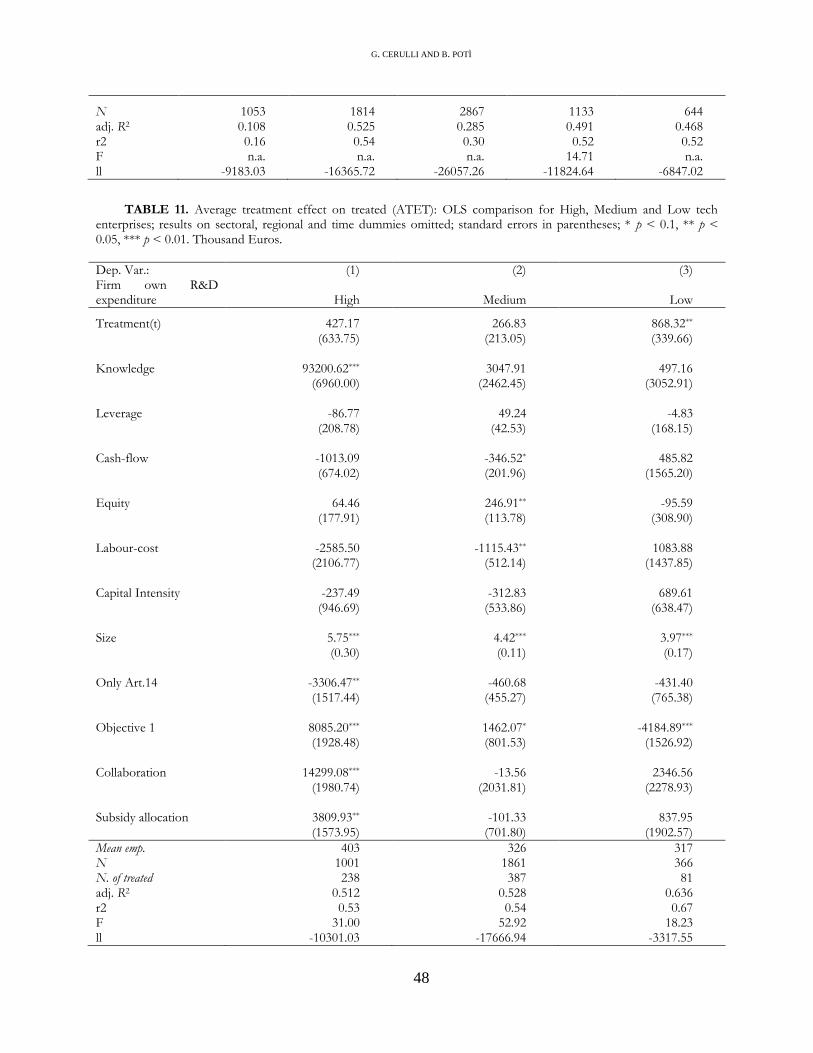
G. CERULLI AND B. POTÌ
48
N 1053 1814 2867 1133 644 adj. R2 0.108 0.525 0.285 0.491 0.468 r2 0.16 0.54 0.30 0.52 0.52 F n.a. n.a. n.a. 14.71 n.a. ll -9183.03 -16365.72 -26057.26 -11824.64 -6847.02
TABLE 11. Average treatment effect on treated (ATET): OLS comparison for High, Medium and Low tech enterprises; results on sectoral, regional and time dummies omitted; standard errors in parentheses; * p < 0.1, ** p < 0.05, *** p < 0.01. Thousand Euros.
Dep. Var.: (1) (2) (3) Firm own R&D expenditure
High
Medium
Low
Treatment(t) 427.17 266.83 868.32** (633.75) (213.05) (339.66) Knowledge 93200.62*** 3047.91 497.16 (6960.00) (2462.45) (3052.91) Leverage -86.77 49.24 -4.83 (208.78) (42.53) (168.15) Cash-flow -1013.09 -346.52* 485.82 (674.02) (201.96) (1565.20) Equity 64.46 246.91** -95.59 (177.91) (113.78) (308.90) Labour-cost -2585.50 -1115.43** 1083.88 (2106.77) (512.14) (1437.85) Capital Intensity -237.49 -312.83 689.61 (946.69) (533.86) (638.47) Size 5.75*** 4.42*** 3.97*** (0.30) (0.11) (0.17) Only Art.14 -3306.47** -460.68 -431.40 (1517.44) (455.27) (765.38) Objective 1 8085.20*** 1462.07* -4184.89*** (1928.48) (801.53) (1526.92) Collaboration 14299.08*** -13.56 2346.56 (1980.74) (2031.81) (2278.93) Subsidy allocation 3809.93** -101.33 837.95 (1573.95) (701.80) (1902.57)
Mean emp. N
403 1001
326 1861
317 366
N. of treated adj. R2
238 0.512
387 0.528
81 0.636
r2 0.53 0.54 0.67 F 31.00 52.92 18.23 ll -10301.03 -17666.94 -3317.55
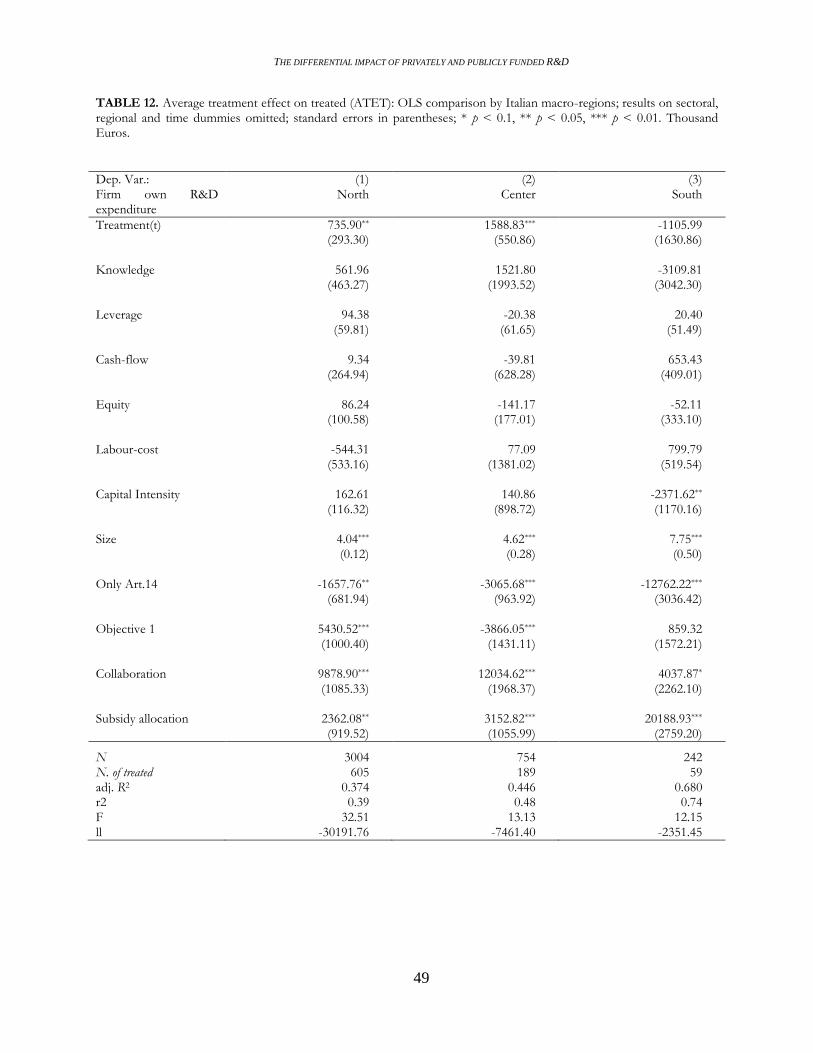
THE DIFFERENTIAL IMPACT OF PRIVATELY AND PUBLICLY FUNDED R&D
49
TABLE 12. Average treatment effect on treated (ATET): OLS comparison by Italian macro-regions; results on sectoral, regional and time dummies omitted; standard errors in parentheses; * p < 0.1, ** p < 0.05, *** p < 0.01. Thousand Euros.
Dep. Var.: (1) (2) (3) Firm own R&D expenditure
North Center South
Treatment(t) 735.90** 1588.83*** -1105.99 (293.30) (550.86) (1630.86) Knowledge 561.96 1521.80 -3109.81 (463.27) (1993.52) (3042.30) Leverage 94.38 -20.38 20.40 (59.81) (61.65) (51.49) Cash-flow 9.34 -39.81 653.43 (264.94) (628.28) (409.01) Equity 86.24 -141.17 -52.11 (100.58) (177.01) (333.10) Labour-cost -544.31 77.09 799.79 (533.16) (1381.02) (519.54) Capital Intensity 162.61 140.86 -2371.62** (116.32) (898.72) (1170.16) Size 4.04*** 4.62*** 7.75*** (0.12) (0.28) (0.50) Only Art.14 -1657.76** -3065.68*** -12762.22*** (681.94) (963.92) (3036.42) Objective 1 5430.52*** -3866.05*** 859.32 (1000.40) (1431.11) (1572.21) Collaboration 9878.90*** 12034.62*** 4037.87* (1085.33) (1968.37) (2262.10) Subsidy allocation 2362.08** 3152.82*** 20188.93*** (919.52) (1055.99) (2759.20)
N 3004 754 242 N. of treated adj. R2
605 0.374
189 0.446
59 0.680
r2 0.39 0.48 0.74 F 32.51 13.13 12.15 ll -30191.76 -7461.40 -2351.45
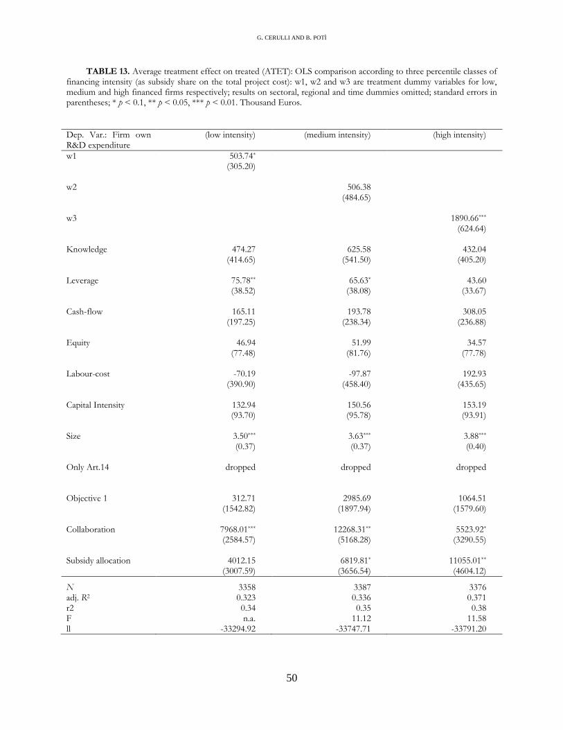
G. CERULLI AND B. POTÌ
50
TABLE 13. Average treatment effect on treated (ATET): OLS comparison according to three percentile classes of financing intensity (as subsidy share on the total project cost): w1, w2 and w3 are treatment dummy variables for low, medium and high financed firms respectively; results on sectoral, regional and time dummies omitted; standard errors in parentheses; * p < 0.1, ** p < 0.05, *** p < 0.01. Thousand Euros.
Dep. Var.: Firm own R&D expenditure
(low intensity) (medium intensity) (high intensity)
w1 503.74* (305.20) w2 506.38 (484.65) w3 1890.66*** (624.64) Knowledge 474.27 625.58 432.04 (414.65) (541.50) (405.20) Leverage 75.78** 65.63* 43.60 (38.52) (38.08) (33.67) Cash-flow 165.11 193.78 308.05 (197.25) (238.34) (236.88) Equity 46.94 51.99 34.57 (77.48) (81.76) (77.78) Labour-cost -70.19 -97.87 192.93 (390.90) (458.40) (435.65) Capital Intensity 132.94 150.56 153.19 (93.70) (95.78) (93.91) Size 3.50*** 3.63*** 3.88*** (0.37) (0.37) (0.40) Only Art.14 dropped dropped dropped Objective 1 312.71 2985.69 1064.51 (1542.82) (1897.94) (1579.60) Collaboration 7968.01*** 12268.31** 5523.92* (2584.57) (5168.28) (3290.55) Subsidy allocation 4012.15 6819.81* 11055.01** (3007.59) (3656.54) (4604.12)
N 3358 3387 3376 adj. R2 0.323 0.336 0.371 r2 0.34 0.35 0.38 F n.a. 11.12 11.58 ll -33294.92 -33747.71 -33791.20
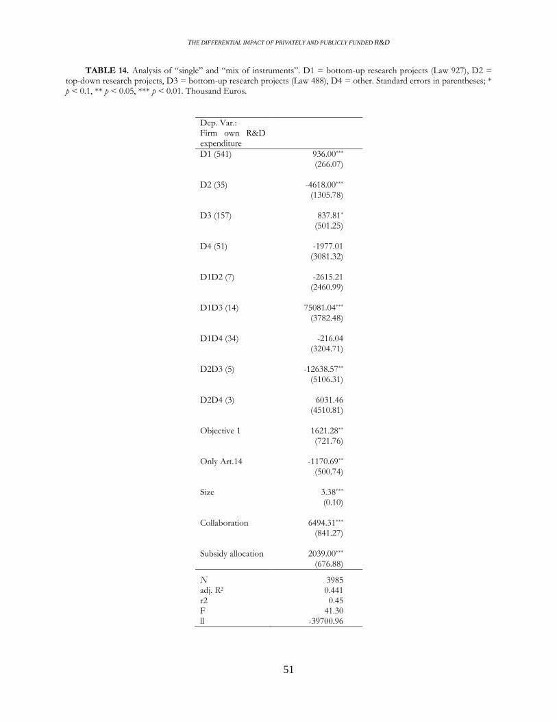
THE DIFFERENTIAL IMPACT OF PRIVATELY AND PUBLICLY FUNDED R&D
51
TABLE 14. Analysis of “single” and “mix of instruments”. D1 = bottom-up research projects (Law 927), D2 = top-down research projects, D3 = bottom-up research projects (Law 488), D4 = other. Standard errors in parentheses; * p < 0.1, ** p < 0.05, *** p < 0.01. Thousand Euros.
Dep. Var.: Firm own R&D expenditure
D1 (541) 936.00*** (266.07) D2 (35) -4618.00*** (1305.78) D3 (157) 837.81* (501.25) D4 (51) -1977.01 (3081.32) D1D2 (7) -2615.21 (2460.99) D1D3 (14) 75081.04*** (3782.48) D1D4 (34) -216.04 (3204.71) D2D3 (5) -12638.57** (5106.31) D2D4 (3) 6031.46 (4510.81) Objective 1 1621.28** (721.76) Only Art.14 -1170.69** (500.74) Size 3.38*** (0.10) Collaboration 6494.31*** (841.27) Subsidy allocation 2039.00*** (676.88)
N 3985 adj. R2 0.441 r2 0.45 F 41.30 ll -39700.96
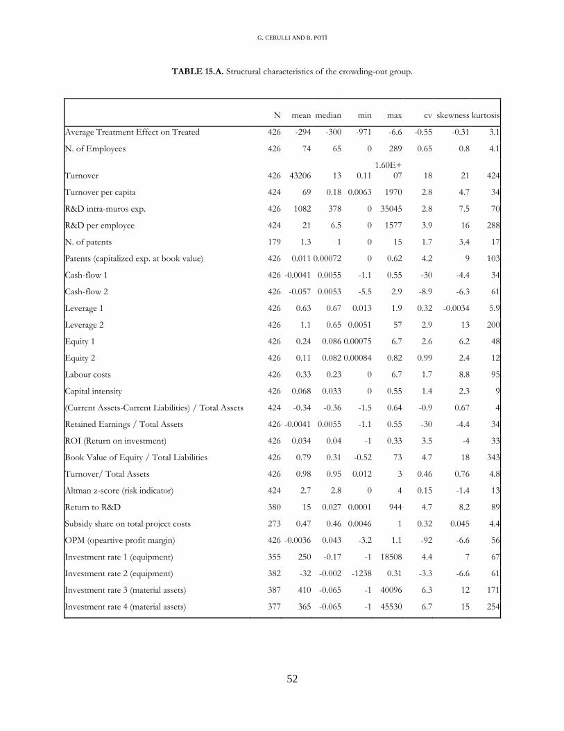
G. CERULLI AND B. POTÌ
52
TABLE 15.A. Structural characteristics of the crowding-out group.
N mean median min max cv skewness
kurtosis
Average Treatment Effect on Treated 426 -294 -300 -971 -6.6 -0.55 -0.31 3.1
N. of Employees 426 74 65 0 289 0.65 0.8 4.1
Turnover 426 43206 13 0.11 1.60E+
07 18 21 424
Turnover per capita 424 69 0.18 0.0063 1970 2.8 4.7 34
R&D intra-muros exp. 426 1082 378 0 35045 2.8 7.5 70
R&D per employee 424 21 6.5 0 1577 3.9 16 288
N. of patents 179 1.3 1 0 15 1.7 3.4 17
Patents (capitalized exp. at book value) 426 0.011 0.00072 0 0.62 4.2 9 103
Cash-flow 1 426 -0.0041 0.0055 -1.1 0.55 -30 -4.4 34
Cash-flow 2 426 -0.057 0.0053 -5.5 2.9 -8.9 -6.3 61
Leverage 1 426 0.63 0.67 0.013 1.9 0.32 -0.0034 5.9
Leverage 2 426 1.1 0.65 0.0051 57 2.9 13 200
Equity 1 426 0.24 0.086 0.00075 6.7 2.6 6.2 48
Equity 2 426 0.11 0.082 0.00084 0.82 0.99 2.4 12
Labour costs 426 0.33 0.23 0 6.7 1.7 8.8 95
Capital intensity 426 0.068 0.033 0 0.55 1.4 2.3 9
(Current Assets-Current Liabilities) / Total Assets 424 -0.34 -0.36 -1.5 0.64 -0.9 0.67 4
Retained Earnings / Total Assets 426 -0.0041 0.0055 -1.1 0.55 -30 -4.4 34
ROI (Return on investment) 426 0.034 0.04 -1 0.33 3.5 -4 33
Book Value of Equity / Total Liabilities 426 0.79 0.31 -0.52 73 4.7 18 343
Turnover/ Total Assets 426 0.98 0.95 0.012 3 0.46 0.76 4.8
Altman z-score (risk indicator) 424 2.7 2.8 0 4 0.15 -1.4 13
Return to R&D 380 15 0.027 0.0001 944 4.7 8.2 89
Subsidy share on total project costs 273 0.47 0.46 0.0046 1 0.32 0.045 4.4
OPM (opeartive profit margin) 426 -0.0036 0.043 -3.2 1.1 -92 -6.6 56
Investment rate 1 (equipment) 355 250 -0.17 -1 18508 4.4 7 67
Investment rate 2 (equipment) 382 -32 -0.002 -1238 0.31 -3.3 -6.6 61
Investment rate 3 (material assets) 387 410 -0.065 -1 40096 6.3 12 171
Investment rate 4 (material assets) 377 365 -0.065 -1 45530 6.7 15 254
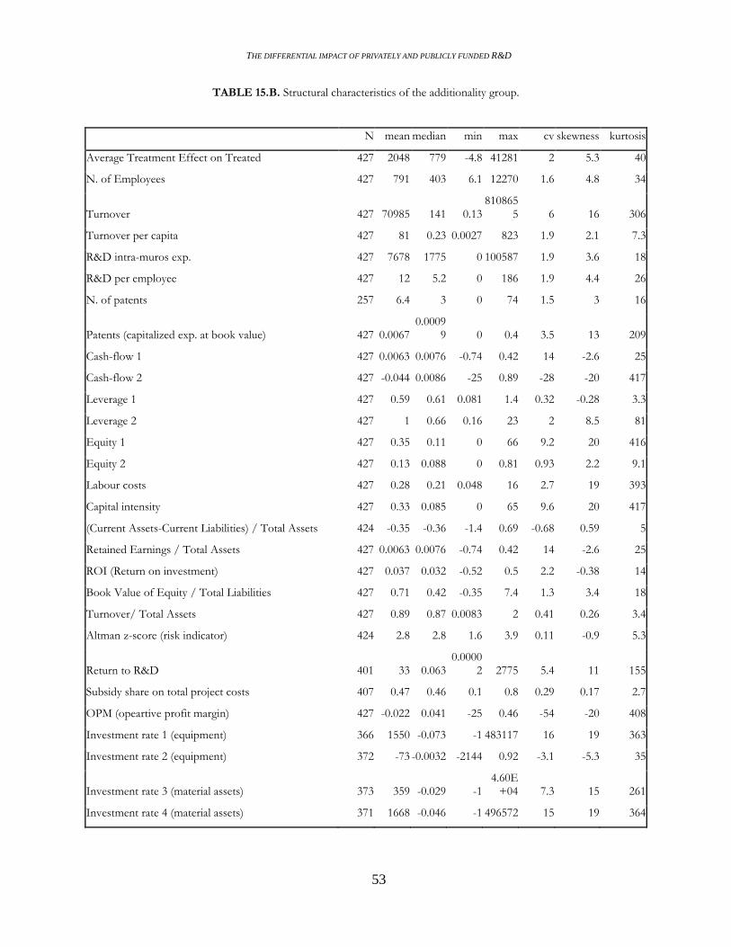
THE DIFFERENTIAL IMPACT OF PRIVATELY AND PUBLICLY FUNDED R&D
53
TABLE 15.B. Structural characteristics of the additionality group.
N mean median min max cv skewness kurtosis
Average Treatment Effect on Treated 427 2048 779 -4.8 41281 2 5.3 40
N. of Employees 427 791 403 6.1 12270 1.6 4.8 34
Turnover 427 70985 141 0.13 810865
5 6 16 306
Turnover per capita 427 81 0.23 0.0027 823 1.9 2.1 7.3
R&D intra-muros exp. 427 7678 1775 0 100587 1.9 3.6 18
R&D per employee 427 12 5.2 0 186 1.9 4.4 26
N. of patents 257 6.4 3 0 74 1.5 3 16
Patents (capitalized exp. at book value) 427 0.0067 0.0009
9 0 0.4 3.5 13 209
Cash-flow 1 427 0.0063 0.0076 -0.74 0.42 14 -2.6 25
Cash-flow 2 427 -0.044 0.0086 -25 0.89 -28 -20 417
Leverage 1 427 0.59 0.61 0.081 1.4 0.32 -0.28 3.3
Leverage 2 427 1 0.66 0.16 23 2 8.5 81
Equity 1 427 0.35 0.11 0 66 9.2 20 416
Equity 2 427 0.13 0.088 0 0.81 0.93 2.2 9.1
Labour costs 427 0.28 0.21 0.048 16 2.7 19 393
Capital intensity 427 0.33 0.085 0 65 9.6 20 417
(Current Assets-Current Liabilities) / Total Assets 424 -0.35 -0.36 -1.4 0.69 -0.68 0.59 5
Retained Earnings / Total Assets 427 0.0063 0.0076 -0.74 0.42 14 -2.6 25
ROI (Return on investment) 427 0.037 0.032 -0.52 0.5 2.2 -0.38 14
Book Value of Equity / Total Liabilities 427 0.71 0.42 -0.35 7.4 1.3 3.4 18
Turnover/ Total Assets 427 0.89 0.87 0.0083 2 0.41 0.26 3.4
Altman z-score (risk indicator) 424 2.8 2.8 1.6 3.9 0.11 -0.9 5.3
Return to R&D 401 33 0.063 0.0000
2 2775 5.4 11 155
Subsidy share on total project costs 407 0.47 0.46 0.1 0.8 0.29 0.17 2.7
OPM (opeartive profit margin) 427 -0.022 0.041 -25 0.46 -54 -20 408
Investment rate 1 (equipment) 366 1550 -0.073 -1 483117 16 19 363
Investment rate 2 (equipment) 372 -73 -0.0032 -2144 0.92 -3.1 -5.3 35
Investment rate 3 (material assets) 373 359 -0.029 -1 4.60E
+04 7.3 15 261
Investment rate 4 (material assets) 371 1668 -0.046 -1 496572 15 19 364
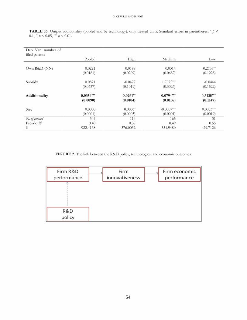
G. CERULLI AND B. POTÌ
54
TABLE 16. Output additionality (pooled and by technology): only treated units. Standard errors in parentheses; * p < 0.1, ** p < 0.05, *** p < 0.01.
Dep. Var.: number of filed patents
Pooled High Medium Low
Own R&D (NN) 0.0221 0.0199 0.0314 0.2733** (0.0181) (0.0209) (0.0682) (0.1228) Subsidy 0.0871 -0.0477 1.7072*** -0.0444 (0.0637) (0.1019) (0.3026) (0.1522) Additionality 0.0354*** 0.0261** 0.0794*** 0.3135*** (0.0090) (0.0104) (0.0156) (0.1147) Size 0.0000 0.0006* -0.0007*** 0.0053*** (0.0001) (0.0003) (0.0001) (0.0019)
N. of treated 344 114 165 31 Pseudo R2 0.40 0.37 0.49 0.55 ll -922.4168 -376.0032 -331.9480 -29.7126
FIGURE 2. The link between the R&D policy, technological and economic outcomes.
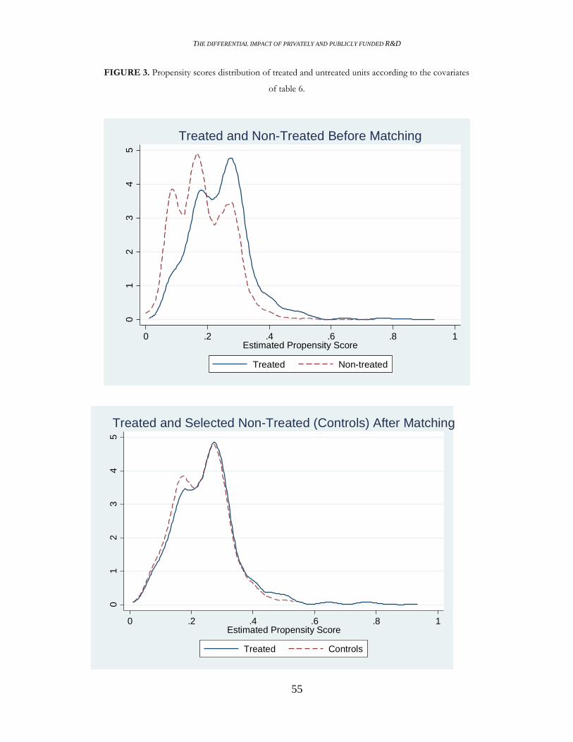
THE DIFFERENTIAL IMPACT OF PRIVATELY AND PUBLICLY FUNDED R&D
55
FIGURE 3. Propensity scores distribution of treated and untreated units according to the covariates
of table 6.
01
23
45
Kern
el d
en
sity
0 .2 .4 .6 .8 1Estimated Propensity Score
Treated Non-treated
Treated and Non-Treated Before Matching
01
23
45
Kern
el d
en
sity
0 .2 .4 .6 .8 1Estimated Propensity Score
Treated Controls
Treated and Selected Non-Treated (Controls) After Matching
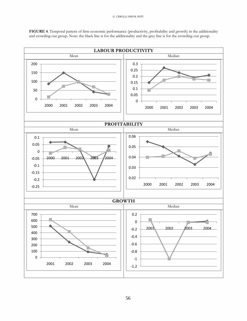
G. CERULLI AND B. POTÌ
56
FIGURE 4. Temporal pattern of firm economic performance (productivity, profitability and growth) in the additionality and crowding-out group. Note: the black line is for the additionality and the grey line is for the crowding-out group.
LABOUR PRODUCTIVITY Mean Median
PROFITABILITY Mean Median
GROWTH Mean Median
0
50
100
150
200
2000 2001 2002 2003 20040
0.05
0.1
0.15
0.2
0.25
0.3
2000 2001 2002 2003 2004
-0.25
-0.2
-0.15
-0.1
-0.05
0
0.05
0.1
2000 2001 2002 2003 2004
0.02
0.03
0.04
0.05
0.06
2000 2001 2002 2003 2004
0
100
200
300
400
500
600
700
2001 2002 2003 2004-1.2
-1
-0.8
-0.6
-0.4
-0.2
0
0.2
2001 2002 2003 2004


![@aa SRT\d >R^ReR d]R^d 64 - Daily Pioneer](https://static.fdokumen.com/doc/165x107/632df348c95f46bf4c073a3c/aa-srtd-rrer-drd-64-daily-pioneer.jpg)