THE DERIVE - NEWSLETTER #23 USER GROUP - Austromath

THE DERIVE - NEWSLETTER #23 ISSN 1990-7079

T H E B U L L E T I N O F T H E

U S E R G R O U P

C o n t e n t s: 1 Letter of the Editor 2 Editorial - Preview 3 DERIVE User Forum (including JORDAN.MTH) Nurit Zehavi and David Ben-Chaim 9 Visualizing a Special Line in the 3D Space G P Speck 13 Some Notes on DERIVE 2.6´s Functions and Limits Josef Böhm 22 The Trigonometric Super Box Bernhard Wadsack 31 DREIECK.MTH - TRIANGLE.MTH (2) Carl Leinbach & Marvin Brubaker 37 Carl ’s and Marvin’s Laboratory (3) 41 ERF-Functions and DERIVE’s Plotting Accuracy 43 ACDC 2 Johann Wiesenbauer 46 Titbits (8) B.Kutzler, B.Waits & F.Demana 49 The TI-92 Corner (W.Pröpper, C.Leinbach, M.Brubaker)

revised version 2010 September 1996

D-N-L#23

I N F O R M A T I O N - B o o k S h e l f

D-N-L#23

[1] Exámenes con DERIVE, José Luis Llorens Fuster DERISOFT (FAX: 907 330 371), 214 pages, ISBN 84-921694-1-9

[2] DERIVE: Aplicaciones matemáticas para PC, Carrillo & Llamas RA-MA, Madrid, 1994

[3] Cómo hacer Matematicás con DERIVE, Castro Chadid Reverté Colombiana, 1993

[4] Aplicaciones de DERIVE: Análisis Matemático-I (Cálculo), J.L.Llorens Fuster Servicio de Publicaciones de la Universidad Politécnica de Valencia, ref. 93735. Valencia, 1993

[5] Aplicaciones de DERIVE: Álgebra Lineal (Fundamentos), J.L.Llorens Fuster Public. de la Universidad Politécnica de Valencia, ref. 94753. Valencia, 1994

[6] Introducción al uso de DERIVE: Aplicaciones al Àlgebra Lineal y Cálculo Infinitesimal, J.L.Llorens Fuster, Public. de la Universidad Politécnica de Valencia, ref. 95638. Valencia, 1995

[7] Cálculo Matemático con DERIVE para PC, Paulorrogàn & .Pérez, RA-MA, Madrid, 1994

[9] Analysis mit DERIVE, Lehr- und Arbeitsbuch für die Jahrgangsstufe 11/1, Hans Jürgen Kayser Dümmler Verlag, 1996, 157 Seiten, ISBN 3-427-45231-X; Dümmlerbuch 4523

Ich erhielt mehrere Anfragen, da das Buch von Larry Gilligan "Mastering the TI-92" für den deutschen Sprachraum offensichtlich schwer erhältlich sein soll. Die ISBN ist 0-9626661-9-X, erschienen bei GILMAR Publishing, P.O.Box 6376, Cincinnati, OH 45206, USA. Sie können das Buch aber noch bequemer erwerben bei bk-teachware, FAX ++43 (0)7236 6065 80.

Exchange for DERIVE - Teaching materials in the DNL.

The wheel has not to be invented twice.

Börse für DERIVE Unterrichts- materialien im DNL.

Das Rad muss nicht zweimal erfunden werden.

I can offer: Binomial Theorem, GCD & LCM, System of coordinates, Modelling Word problems with DERIVE (all in English and German), SET.EXE, MENGE.EXE (a program to teach and to practise operations with sets including VENN diagrams, in English and German). I have produced a paper „Einführung in die Matrizenrechnung mit DERIVE“ - in German. If you are interested I would send you the paper on a diskette in MSWord6-format.

This is DfW

DERIVE for WINDOWS.

The first screen shot using DfW, de-monstrating an ALGEBRA- and a PLOT window.

One of the new features: You are able to add annotations to your plots.

D-N-L#23

L E T T E R O F T H E E D I T O R

p 1

Liebe DUG Mitglieder, Es war wirklich schön, so viele von Ihnen in Bonn zu tref-fen oder persönlich kennen zu lernen. Fast alle, die zum ersten Mal eine DERIVE Konferenz besuchten, waren einmal mehr begeistert von der familiären Atmosphäre, vom hohen Niveau und vom ungebrochenen Enthusiasmus der Teilnehmer. Sie haben es genossen, mit David Stoute-myer, mit Bert Waits, um nur zwei zu nennen, und vielen anderen, die sie aus dem DNL kennen, zu sprechen und zu diskutieren. Ich wurde einige Male angesprochen: "Josef, zeige mir bitte den ..., ich möchte doch wirklich wissen, wer das ist!"

Nicht nur J.Wiesenbauer nahm einige Ideen von Bonn nach Hause. Auch Josef Lechner und Eugenio Roanes haben ihre Kontakte vertieft und sind nun dabei, gemeinsam, LOGO in DERIVE zu imple-mentieren. Leider konnte ich bei so vielen Vorträgen nicht, die mich interessiert hätten nicht dabei sein, aber dafür freue ich mich auf den Tagungsband.

Abschließend möchte ich namens der DUG den beiden Organisatoren, Bärbel Barzel und Leo Klingen für Ihre große Mühe herzlich danken.

Vor Bonn hatte ich die Gelegenheit, an einer T3-Ausbildung - Teachers Training for Technology - in Columbus, Ohio, teilzunehmen. Diese, von B.Waits und F.Demana gegründe-te Initiative soll nun unter anderem auch auf Europa aus-gedehnt werden. Bei dieser Gelegenheit darf ich Sie ersu-chen, TI-92 Beiträge an Bert Waits oder an mich zu schi-cken. (Vergessen Sie aber bitte nicht das klassische DERIVE!)

Thomas Weth kommt mit seinem Kurvenlexikon wieder im nächsten DNL zu Wort. Gerade bei seinen Beiträgen lässt sich eine sinnvolle Verbindung zwischen einem CAS und der interaktiven Geometrie sowohl auf dem PC als auch auf dem TI-92 herstellen.

Ich möchte Sie nochmals darauf hinweisen, dass Sie die .MTH-files zu diesem DNL von SWHH´s web page herunter laden können. Danke, Al Rich. Vom renommierten Verlag BIRKHÄUSER AG wurde ich gebeten, für unsere deutschsprachigen Mitglieder eine Information über die Fachzeitschrift "Elemente der Ma-thematik" beizulegen. Diesem Wunsch komme ich gerne nach. Bis zum nächsten DNL - der „Weihnachtsnummer" mit einigen Zugaben - grüßt Sie herzlichst Josef Böhm

Nur für Eingeweihte: Habt Ihr das Mäppchen gefunden?

Dear DUG Members, It was really nice to meet so many of you in Bonn and to make your acquaintance. Most of those who at-tended a DERIVE Conference the first time were fascinated from the familiar atmosphere, the high level and the unbroken enthusiasm of the participants. They enjoyed talking, discussing and joking with David Stoutemyer and Bert Waits, to mention two people, and with many others who they were knowing from the DNL. It happened several times that I was asked "Oh, Josef, please show me ......., I really would like to know who he (she) is!"

Not only Johann Wiesenbauer took some ideas back home. Josef Lechner and Eugenio Roanes for example, have renewed their contacts and are now busy to implement LOGO in DERIVE. Unfortunately I was not able to attend all the lectures I was inter-ested in. But I am looking forward to studying the Proceedings. Finally I want to express many thanks on behalf of the DUG to the organizers, Bärbel Barzel and Leo Klingen for their tremendous efforts to make our stay in Bonn as pleasant as possible.

The week before Bonn I had the possibility to attend a T3 - Conference - Teachers Training for Technology - in Columbus, Ohio. T3, founded by B.Waits and F.Demana will be established now in Europe, too. On this occasion I’d like to invite you to submit TI-92 pa-pers to B.Waits, B.Kutzler or to me. (But don’t forget the classic DERIVE!) Thomas Weth will continue his "Lexicon of Curves" in the next issue. Especially his articles are excellent examples how to link a CAS with interactive geometry which can be realized now on a PC as well as on the TI-92. I want to point out once more that you can download the .MTH-files belonging to this issue from SWHH´s web page. Many thanks, Al Rich. Until the next DNL - the "Christmas Issue" with some extras -

Sincerely yours Josef Böhm

Tangrams w i th DERIVE

(in one of the next ACDCs)

p 2

E D I T O R I A L

D-N-L#23

The DERIVE-NEWSLETTER is the Bulle-tin of the DERIVE User Group. It is pub-lished at least four times a year with con-tents of 40 pages minimum. The goals of the DNL are to enable the exchange of ex-periences made with DERIVE as well as to create a group to discuss the possibilities of new methodical and didactical manners in teaching mathematics. We include now a section dealing with the use of the TI-92.

Editor: Mag. Josef Böhm A-3042 Würmla D´Lust 1 Austria Phone/FAX: 43-(0)660 3136365 e-mail: [email protected]

Contributions: Please send all contributions to the Editor. Non-English speakers are encouraged to write their contributions in English to rein-force the international touch of the DNL. It must be said, though, that non-English articles will be warmly welcomed nonethe-less. Your contributions will be edited but not assessed. By submitting articles the author gives his consent for reprinting it in the DNL. The more contributions you will send, the more lively and richer in contents the DERIVE Newsletter will be.

Preview: Contributions for the next issues Graphic Integration, Linear Programming, Böhm, AUT LOGO in DERIVE, Lechner & Roanes Lozano, AUT & ESP 3D-Geometry, Reichel, AUT Parallel- and Central Projection, Böhm, AUT Algebra at A-Level, Goldstein, UK Tilgung fremderregter Schwingungen, Klingen, GER A Utility file for complex dynamic systems, Lechner, AUT Examples for Statistics, Roeloffs, NL Linear Mappings and Computer Graphics, Kümmel, GER Solving Word problems (Textaufgaben) with DERIVE, Böhm, AUT DERIVE and ACROSPIN, Schorn & Böhm, AUT/GER Line Searching with DERIVE, Collie, UK About the "Cesaro Glove-Osculant", Halprin, AUS 3rd-order Differential Equations, Guitiérez, ESP Tangrams with DERIVE, Población, ESP The TI-92 Section, Waits a.o. and Setif, FRA; Vermeylen, Belgium; Leinbach, USA; Halprin, AUS Weth, GER; Wiesenbauer, AUT; Keunecke, GER; Aue, GER;

Weller; GER, Stahl, USA; Mitic, UK; Koth, AUT; and .......

Impressum: Medieninhaber: DERIVE User Group, A-3042 Würmla, D´Lust 1, AUSTRIA Richtung: Fachzeitschrift Herausgeber: Mag. Josef Böhm Herstellung: Selbstverlag

D-N-L#23

D E R I V E - U S E R - F O R U M

p 3

Victor Hermans, Voorschoten, Netherlands We have recently met at the DERIVE Conference in Bonn. I liked the atmosphere very much and I have found a few colleagues teaching the same subjects as I do. My favourite interest is financial math. I have recently visited the ICME at Sevilla and last year I was at the CIAEM Conference at Berlin and there was no lecture on financial math. The subject seems too practical for mathematicians and too difficult for economists. So my ques-tion is: could we start a user group of financial math teachers, whatever the platform? Personally, I have tried to do this in Holland - with Hewlett-Packard financial calculators - with no success. People are just not interested in any machine in the classroom. By the way; there are no graphic calculators and there is no DERIVE in Dutch secondary education, and there will not be anything like that on the central examinations for the next four years. ..... ...... DNL:. I think we could establish a "Financial Math Working Group" within the DUG if there are other interested members, too. Or we start the Group as a pair of enthusiasts. I would like to ask you for a "pilot contribution" to make clear some topics for this group. As I am a teacher on a "Handelsa-kademie" (= "College for Business Administration") I am very interested in your idea and I am looking forward to hearing from you in the near future. Jan Vermeylen, Kapellen, Belgium Have you got any experience with the link you can make between DERIVE and the programming language C++? Where could I find more information or examples? DNL: Are there any members with experience in combining DERIVE results and C++-applications. I used very successfully the linkage to BASIC programming ACD.EXE to convert DERIVE results into ACD-files for ACROSPIN. I’ll present this program in the next DNL. Any other applications would be appreciated. George Feeman, Al Ain, United Arab Emirates We have come across this bug in Ver.3.00 and 3.10:

2

32

+−

x x Simplifies to −

+6

3x x( )

2

33

1+−

+x x Simplifies to −

++ +

xx x

71 3( )( )

and so on, but

2

33

+−

x x DOES NOT Simplify - the output is the same expression.

Can you tell me why? Why this exception to this simple algorithm? DNL: At the occasion of the Bonn DERIVE Conference I discussed this "bug" simplifying the sum of two simple rational expressions with David Stoutemyer. By the way: that’s not a "bug" of only DERIVE 3.x versions. DERIVE 2.58 returns the same results. That’s a summary of David’s answer: Computer Algebra is among others the art of recognizing and using patterns. DERIVE always looks for patterns to apply any simplification. (Josef’s question: "What is the definition of simple???")

In 2

32

+−

x x DERIVE recognizes the same numerators and then tries to apply a rule.

In 2

33

1+−

+x x DERIVE discovers two denominators of the form (x + constant) and then ap-

plies the rule to add two fractions using common denominators, but .......

in 2

33

+−

x x DERIVE cannot find any pattern:

3x

is treated rather as 3 1x− than as 3

x c+

Maybe you will not find this explanation very satisfactory. Nevertheless it is always interesting to look behind the curtain of a CAS.

p 4


D-N-L#23

Helmut Wunderling, Berlin, Germany Anbei Bildschirmausdrucke von DERIVE. Die obe-ren Bilder zeigen, wie unter Softwindows auf einem Powermac die Aufbauroutinen des Bildschirms nicht vollständig funktionieren. Das hat zur Folge, dass bei Ausdrücken, die wechselnd ein- und mehrzeilig sind, die Lesbarkeit dahin ist (vgl. Ausschnitt). Der untere Teil zeigt, dass Version 3.12 die Sonder-zeichen für Integrale, Wurzeln, Summen usw. nicht bereitstellt und zwar auch auf PC (z.B. Hewlett Pa-ckard) und das, obwohl die Version 2.59 z.B. das nun wieder anstandslos tut. Ich bräuchte aber für Veröffentlichungen gute Bilder. Was kann ich tun??

Attached you can find screen dumps of DERIVE. The upper pictures (full screen and part of the screen) show that using Softwindows on a Powermac the building up routines of the screen will not work properly. From this follows that expressions with alternately one and more lines are not readable. The dump on the bottom shows that version 3.12 does not provide the special characters for sum, integral, roots etc, and that even on a PC (Hewlett Packard) al-though I don’t have any problems using 2.59. For a publication I need nice screen dumps. What shall I do???

D-N-L#23


p 5

Miguel de Guzmán, Madrid, Spain I am sending a small program connected with the Jordan form I have described by email. I presume that somebody has thought of this before. Otherwise perhaps it would be useful for some people.

Dada a y un autovalor z se escribe BLOQ_JORDAN(a,z) y resulta un vector de numeros enteros no negativos [numero de cajas de dimension 1, numero de cajas de dimension 2, .....]

p 6


D-N-L#23

______________________________________________________ References: Elementary Linear Algebra with DERIVE, R.J.Hill and T.A.Keagy, Chartwell-Bratt, 1995.

D-N-L#23


p 7

In the following you can see how to transfer this utility to TI-NspireCAS. The rank function is not implemented in the base system but it is available via the linalgcas-library. The screenshots below should be informative enough that you can reproduce the procedure on your own.

p 8


D-N-L#23

For accomplishing this contribution see the same procedures performed with the TI-92 / Voyage 200.

D-N-L#23

Nurit Zehavi & David Ben-Chaim: A Special Line

p 9

Visualizing a Special Line in the 3-D Space

Nurit Zehavi & David Ben-Chaim Weizmann Institute of Science, Israel

The motivation The second author shared with the first author a paper that he had submitted for publication, entitled, A Special Point in the 2-D Plane and a Special Line in the 3-D Space. The paper ex-plores systems of linear equations that are written in the standard form with coefficients oc-curring as consecutive terms of arithmetic sequences. He challenged her: Can we prepare an activity for teachers based on this paper using Derive? The result It is easy to verify, algebraically and graphically, that the ordered pair (-1, 2) satisfies any linear equation in two variables that when written in the standard form the coefficients are consecutive numbers from an arithmetic sequence.1)

The solution of the general 3-by-3 system of linear equations with arithmetic sequences for coefficients ,

a1.x + (a1 + d1)y + (a1 + 2d1)z = a1 + 3d1 a2.x + (a2 + d2)y + (a2 + 2d2)z = a2 + 3d2 a3.x + (a3 + d3)y + (a3 + 2d3)z = a3 + 3d3

is parametric [@1, -2@1 - 1, @1 +2].

The graphical representation of a linear equation in three variables is a plane. The interpreta-tion of the algebraic solution above is that all the planes that represent equations with "arith-metic coefficients" intersect in a Special Line (t, -2t – 1, t + 2) (choosing t to be the parame-ter). How can we demonstrate this finding applying Derive?

Derive can place only one surface at a time in the 3D-plot window. However, we superim-posed several planes in Acrospin and watched for the intersection line while running Acro-spin. The special line in this representation was not very convincing. Coincidentally we re-ceived the card from Soft Warehouse with an invitation to "surf" the net to their web page. In the Derive-Questions-and-Answers section it was suggested to plot the minimum of two sur-faces in order to see their intersection. Aha!

We applied the method to an example taken from Ben-Chaim's paper:

x + y + z = 1 x + 7y + 13z = 19 5x + y - 3z = -7

The equations were modified to the explicit form z = u(x, y) and the minimum of the three planes was plotted (see figure 1). The following figures were plotted by teachers who ex-plored the situation. In figure 2 the first equation was replaced by another one with arithmetic coefficients, x - z = -2, and the special line appeared again. But do we see the same picture? Some teachers studied the 3D plots and compared coefficients, others ran the Acrospin file (it

P 10


D-N-L#23

is helpful to plot each of the three planes in a different colour), and a few issued the dot prod-uct of the vectors orthogonal to each of the planes and compared the angles between the planes. In figure 3, the first equation was replaced by z = y so that the three planes intersect in one point (-1, 1, 1). Now a question was raised: Is it possible to see the special line even if one of the equations does not fulfil the arithmetic coefficients condition?

Figure 1 MIN(-x-y+1,-(x+7y-19)......) Figure 2

D-N-L#23


p 11

The equations , ax + by + cz = d, to consider must be represented by planes that are parallel to the identified special line [0, -1, 2] + t[1, -2, 1] (written in vector notation). Thus the dot prod-uct [1, -2, 1].[a, b, c] = a -2b + c must be zero. In figure 4 such equation, z = x, was chosen to replace the middle equation. Not surprisingly, the plot in figure 5 is the same as in figure 1, but the coefficients of x + y + z = 10 are not consecutive numbers of an arithmetic sequence. In fact, the plane that represents x + y + z = 10 is parallel to one of the planes seen in figure 5. In conclusion, the special line activity provides opportunities for teachers to revise and extend their knowledge by using the possibilities offered by the software.

Figure 4 Figure 5

Nurit and David mentioned in their paper the ACROSPIN animation of their objects. As some of you might not know how to combine several DERIVE 3D-plots in different layers and colours in one ACROSPIN-file I’ll explain how to do: Edit the first plane: pl1:=-x-y+1, Plot the grid in an appropriate colour (Grids 20) in the 3D-plot window and then press Transfer Acro-spin Save: MYNAME. Now you may Run Acrospin to view your result so far. Switch back to the Alge-bra window, highlight or edit the second plane: pl2:=-(x+7*y-19)/13

p 12


D-N-L#23

Plot it again in an appropriate colour. Then Transfer Acrospin Save, confirm MYNAME.ACD pressing ·. Skip "Overwrite existing file" pressing N and confirm "Append to existing file" pressing Y. Then go back once more to the Algebra window and repeat the same procedure once more with the third plane. pl3:=(5*x+y+7)/3 Now run Acrospin.

The right Acrospin animation containing the planes together with the intersection line was produced using my ACD.EXE tool. (Next DNL!!). Josef _____________________________________________________________________ 1) E. Sawada, Extending Algebra Concepts with Technology, DNL#12, December 1993

D-N-L#23

G P Speck: Some Notes on DERIVE´s Limits

p 13

Some Notes on DERIVE 2.6´s Functions and Limits

G P Speck, Wanganui, New Zealand

Using DERIVE 2.6, we have the following results for specific functions, as shown on the printout be-longing to these examples:

(If there are any differences using other - more recent - DERIVE versions I’ve added them. Maybe that Al Rich or David Stoutemyer will have some comments on Mr Speck’s paper?)

Example 1: F1(x) = x SIN(1/x). For this function F1(x), all of the DERIVE 2.6 functional values and limits agree with the classical results; e.g., lim F1(x) as x → 0+ = lim F1(x) as x → 0– = lim F1(x) as x → 0.

Example 2: F2(x) = IF(x = 0, 5, x SIN(1/x)). For this function F2(x), we have the following DERIVE 2.6 limit results. We see that each of these results DISAGREE with the corresponding classical calcu-lus limit results. each of which is 0 if we work with approXimate. The function F(x):=IF(x=0,0,x SIN(1/x)) has all limits equal to 0 as x tends to 0, as it is the case for the classical limits.

p 14


D-N-L#23

Example 3:

F3(x) = IF(x > 1, IF(x = 0, 0, -1)). For this function F3(x), we have the following DERIVE 2.6 limit results. The left and right hand DERIVE 2.60 limits agree with the classical calculus results, but the two-sided DERIVE 2.60 limit DOES NOT AGREE with the classical result.

D-N-L#23


p 15

Example 4: F4(x) = IF(x SIN(π/x) = 0,1,2). For this function F4(x), the DERIVE 2.6 limits with the value 1 DO NOT AGREE with the corresponding classical calculus limits, while those with the value 2 DO AGREE with the classical limits; also the lim F4(x) as x → 0 as given below (in approXimate Mode and if interpreted appropriately) DOES AGREE with the classical calculus limit.

This is from 1996 ┌ 1 1 1 1 │ "x" -î -2 - ─── - ─── - ─── - ───────── 0 │ 2 3 4 1000000 #12: │ │ ┌ ┌ π ┐ │ "F4(x)" 2 2 1 1 1 1 IF│0·SIN│───│ = └ └ └ 0 ┘ 1 1 2 2 2 ┐ ───────── ──── ─── ─── ──── │ 1000000 10 3 9 27 │ │ ┐ │ 0, 1, 2│ 1 1 2 2 2 │ ┘ ┘

p 16


D-N-L#23

Simplify in Version 3.14: ┌ 1 1 1 1 1 │ "x" -î -2 - ─── - ─── - ─── - ───────── 0 ───────── #15: │ 2 3 4 1000000 1000000 │ └ "F4(x)" 2 2 1 1 1 1 1 1 1 2 2 2 ┐ ──── ─── ─── ──── │ 10 3 9 27 │ │ 1 2 2 2 ┘

approXimate in Version 3.14: ┌ 1 -6 -6 2 2 │ "x" -î -2 -0.5 - ─── -0.25 - 10 0 10 0.1 ─── ─── #17: │ 3 3 9 │ └ "F4(x)" 2 2 1 1 1 2 1 2 1 2 2 2 ┐ ──── │ 27 │ │ 2 ┘ In DNL#23 from 1996 follows a thorough investigation of left- and right sided limits. As this is of no importance now I am omitting this part and go ahead with G P Specks 5th example:

Example 5:

F5(x) = | SIGN(x) |. F5(0) = | SIGN(0) |.Simplifies or approXimates to 1, even though SIGN(0) is un-defined and when Simplified or approXimated gives SIGN(0). (note, however, that √ SIGN2(0) returns SIGN(0), as should be the case.). Each of the DERIVE 2.60 limit results DOES AGREE with the cor-responding classical calculus limit. However, the following DERIVE 2.60 derivative results (which are of course special limits) are NOT in agreement with the classical calculus derivative at x = 0.

D-N-L#23


p 17

Example 6:

F6(x, y) = IF(y = x2, 1, 0). Each of the first two DERIVE 2.60 limits below DISAGREES with the cor-responding classical limit for a function of two variables, since the classical calculus limit fails to exist in each case. The third limit below AGREES with the corresponding classical calculus one.

The same comments can made be here for the LIM2 results as were made for the LIM results above. Note that neither the DERIVE 2.60 LIM nor LIM2 (being limits along rays through the point in ques-tion) are designed to handle the classical limit of a function of the F6 type, even in the absence of the difficulties shown here.

p 18


D-N-L#23

A number of the difficulties illustrated in the preceding examples can be traced to the way in which DERIVE 2.60 limits behave relative to functions using the IF( ) statement - however, as Example 5 shows, this is not the only difficulty. The way in which DERIVE 2.60 limits react relative to the IF( ) statement functions given above can be determined without too much analysis; but other more compli-cated multiple IF( ) statement functions can be displayed where it is not nearly so easy to predict just what the DERIVE 2.60 limit result will be. I have created a variety of simple DERIVE "programs" to bypass some of the one and two variable limit difficulties, but have not come up with a totally satisfactory solution to the inherent limit prob-lems. Example 5 above illustrates a particularly annoying problem in that DERIVE returns a numerical value for the composition of two pre-defined functions at an independent variable value which "shouldn’t" be in the domain of the composition. How many other examples of this kind are preva-lent? None? Several? If we were confident that DERIVE will produce appropriate functional values for all predefined and author defined (using IF( ) where needed) functions and compositions of such functions, then we would be in a position to seriously tackle the resolution of the DERIVE limit difficulties. Notwith-standing the difficulties raised herein, for the very great majority of DERIVE functions of whatever type that I have used, correct functional values are returned. As long as this is the case, DERIVE does provide two very powerful tools for investigating important features, including the limit, of non-trivial functions: the easy display of a table of functional values and functional plots. As an illustration, Ex-ample 7 in the printout that follows shows the verification (by way of a table) of an important feature of the very interesting non-analytic function

D-N-L#23


p 19

Example 7: An example of a non-elementary type of local minimum

21-

1( ) ( ) ( ) sin where

( ) ( )2 2( ) and ( ) with

2 2

( ) for 0 and( ) 0 for 0.

x

F x A x B xx

x xC x C C x CA X B x

C x e xF x x

= +

+ − = =

= ≠= =

0

p 20


D-N-L#23

It can be proved for our F(x) defined above for all real x: F(x) has derivatives of all orders at each real x; F(x) has a relative minimum at x = 0; a1 > b1 > c1 and F(c1) < F(a1) < F(b1) for n ≥ 2. Thus, F'(x) is not ≥ 0 throughout any interval (0,b), nor is F'(x) ≤ 0 throughout any interval (a,0). The DERIVE matrices displayed above provide simple verification that a1 > b1 > c1 and F(c1) < F(a1) < F(b1) for 2 ≤ n ≤ 7. Such simple DERIVE verification is very handy indeed in providing confidence in one’s theoretical results for "intricate" functions such as our F(x) given here. The following is a "graphical" view of the relative magnitudes of a1, b1, c1 and F(a1), F(b1), F(c1). F | | for n >= 2: | | * | | | * | | * | | -|----|---------|----|-------- x c1 < b1 < a1 F(c1) < F(a1) < F(b1)

D-N-L#23


p 21

A word of caution! If we define F(x) in the following manner without Simplifying F(x) as was done above, then the matrix of values for F(a1), F(b1) and F(c1) may be totally inaccurate!!

We see that the F(c1) and F(a1) values in this matrix are totally different from the correct function values in the simplified F(x) matrix above, while the F(b1) values agree for the two matrices. A classi-cal problem in numerical analysis underlies the difficulty here: For our function F(x) e^(-4/x^2) is so much smaller than e^(-1/x^2) for a1 with n = 2, for example, that the evaluation of A(a1) with PrecisionDigits: 20 will give the value A(a1) = (4.83347 10^-106)/2 and similarly for B(a1). If we used PrecisionDigits: 100 in this case the following shows that the DERIVE F(a1) value would be the correct value:

p 22

Josef Böhm: The Trigonometric Super Box

D-N-L#23

The Trigonometric Super Box

Josef Böhm, Würmla, Austria

In DNL#9 from March 1993 I presented a "Black Box" to solve oblique triangles. At the occasion preparing a workshop for the DERIVE Conference 1996 I tried to extent this "Black Box" to a real "Superbox" in order to build a "Circuit of Boxes" for this special subject.

For all functions and formulae we define a triangle with common names for sides and angles:

(I based my workshop on the problem:

∆ABC(BC = 120, AC = 80, ∠ABC = 20°)).

This is the most difficult case, because we have to consider two solutions!!

1 The White Box In the White Box phase we would derive the Sine Rule and the Cosine Rule. The scientific pocket calculator is sufficient support at that time. The first step using DERIVE could be editing the Cosine Rule and the Sine Rule. The students must know which of the both rules applies for solving a problem, which variables can be substituted and then let DERIVE solve the respective equation. I’d like to call this position as

2 Not a Box at all The start of solving the given problem could look like as follows: Not a Box at All User: #1: InputMode ≔ Word User: 2 2 2 #2: s3 = s1 + s2 - 2·s1·s2·COS(a3) User: #3: s1·SIN(a2) = s2·SIN(a1) User: #4: 80·SIN(α°) = 120·SIN(20°) Solve(#4,α): #5: SOLVE(80·SIN(α°) = 120·SIN(20°), α, Real) Approx(#5): #6: α = -210.8658824 ∨ α = 149.1341175 ∨ α = 30.86588247

D-N-L#23


p 23

Take care that you set Manage Trigonometry Angle: Radian (in DERIVE 6: Options > Mode Settings > Angular unit > Radians). So you have to substitute for the angle a2 in line #3 α deg. In the next phase we provide four functions which give the solutions of the equations in lines #2 and #3 for the angle or the side. This package of functions represents the

3 The "Gray" Box

cs_a3(side_1, side_2, angle_3) returns side_3 ca_s1(side_1, side_2, side_3) returns angle_1 ss_a2(side_1, angle_1, angle_2) returns side_2 sa_s2(side_1, side_2, angle_1, k) returns angle_2 (k = 1 ⇒ angle_2 ≤ 90°, k = 2 ⇒ 90° < angle_2 ≤ 180°,

k = 1 by default.) The students must still know which of the rules applies. They also have to consider the case with the possibility of obtaining two solutions. To explain the "names" of the functions:

cs_a3 = use the Cosine Rule to find the Side opposite to Angle_3. (You will find the "Gray Box functions" in the DERIVE printout at the end of the contribution.)

4 The "Black Box" These four functions from the "Gray Box" can be developed together with the students. The next ones are more difficult. We use the Gray Box Functions and combine them to a real "Black Box" to solve the triangles in one step. It will depend on the students´ skill in working with DERIVE to produce the next package. This could be much easier if the maths teacher is also the information technology teacher. We can build in some control structures (considering the triangle’s inequality, considering one, two or none solution in case of SSA, ....). I could imagine to produce the most difficult module together with the students and let them produce the remaining ones in groups by their own.

Last year I was short of time teaching trigonometry. I only had time to deal with the trigonometric functions and their applications in connection with right angled triangles. But I didn’t want to miss the applications of solving oblique triangles in plane and space. I wanted the students to use strategies for calculating polygons and problems in 3D-space. So I provided this Black Box in a Utility file and an instruction similar to the following:

Load the Utility file TRIGO.mth. You then will have four functions available for solving triangles. The provided functions are:

sss(side_1, side_2, side_3) sas(side_1, angle_3, side_2) asa(angle_2, side_1, angle_3) ssa(side_1, side_2, angle_1)

(I don’t want to repeat that part from DNL#9. I use these functions for building the SUPER BOX.)

p 24


D-N-L#23

But according to Bernhard Kutzler [2,3] the real Super Box would be a function like

triangle(side_1, side_2, side_3, angle_1, angle_2, angle_3) with three parameters known and three unknown. DERIVE should do all the remaining work: check if the triangle really exists, decide the case and calculate the missing sides and angles. Then our example should look like that:

triangle(120, 80, side_ab, angle_bac, 20°, angle_abc).

I faced the challenge to develop such a function and we reproduced the ideas in the workshop.

5 The "Super Box" Depending on the unknown parameters in TRIANGLE(…) DERIVE has to decide which of the Black Box functions applies. Additionally we want to implement the until now untreated case of SAA. (This is new even for the participants of the Workshop in Bonn). In the Black Box phase we would calculate the third angle by hand and then apply ASA. That is now the moment when not only the - not too dif-ficult - implementing of mathematical rules will take place but when you also - perhaps with your students - have to consider an algorithm. In the following I will present one possibility (I didn’t find a better one):

I set up a table with 6 columns for the parameters and sufficient rows to represent all the possible

combinations to define a triangle from SSS to AAA - (next page). As 63

= 20 we need 20 rows. Sur-

prisingly a pattern emerges. This pattern is the key to solve the problem. The parameters have to be edited as a vector v and the existence of values for its elements creates the code for the application of well known tools. While C2(v) picks out the SAA-case, CODE(v) gives a unique relation between the code numbers and the remaining problems (SSS, ASA, AAA and SSA). The IF-construct returns the value 0 if DERIVE cannot decide whether the expression is 0 or not. And that is the case, if the expression is a not predesignated variable or a given constant value.

c2(v):=IF(v SUB 1*v SUB 4*v SUB 5>=0 OR (v SUB 1*v SUB 4*v SUB 6>=0 OR (v SUB 2*v SUB 4*v SUB 5>=0 OR (v SUB 2*v SUB 5*v SUB 6>=0 OR (v SUB 3*v SUB 4*v SUB 6>=0 OR v SUB 3*v SUB 5*v SUB 6>=0)))),1,0,0)

code(v):=SUM(VECTOR(IF(v SUB i=0,i,i,0),i,6))

For example see some codes:

For the cases SAS and ASA only a permutation of the parameters is necessary. AAA is special: DERIVE returns the proportions of the sides (see one example!). The most difficult problem occurs in the cases of SSA and SAA, because there is no unique relation between the code numbers and the given sides and angles. But as you can see in the special printed numbers in the table there is an unique incidence of pairs of numbers. We can use the fact that the product of these pairs is defined and greater 0 to identify the problem. See first the table followed by some examples :

D-N-L#23


p 25

side_1 = v1 side_2 = v2 side_3 = v3 angle_1=a1 angle_2=a2 angle_3=a3 Σ = Code Case

4 10 SAA 4 11 SAA

5 11 SAA 5 13 SAA 6 13 SAA 6 14 SAA

1 2 3 6 SSS

1 2 6 9 SAS 1 3 5 9 SAS 2 3 4 9 SAS

1 5 6 12 ASA

2 4 6 12 ASA

3 4 5 12 ASA

4 5 6 15 AAA

1 7 SSA

2 8 SSA

2 10 SSA

3 11 SSA

1 8 SSA

3 10 SSA

p 26


D-N-L#23

CIRCUIT OF BOXES The workshop and, of course, this contribution should demonstrate that you are able to "pro-gram" even in DERIVE. You can use control structures and "error catching". There are many possibilities to change from one box phase to another one. I try to illustrate that fact. You can step into this circuit at any position and then move to all directions.

Now, in 2010 with DERIVE 6.10 and its programming features available I would doubtless try writing a compact DERIVE program. There are some differences to the code given in 1996 because of changes in DERIVE´s functionality (e.g. SOLVE in 1996 and SOLVE/SOLUTIONS in later versions). In later versions we can differ between ASIN and ARCSIN. This is also not considered in this package. But the package works as it is.

D-N-L#23


p 27

p 28


D-N-L#23

D-N-L#23


p 29

p 30


D-N-L#23

triangle(v) is the main function. According to the code numbers it assigns each problem to its solu-tion procedure.

There is one more improvement possible. I will try to append the feature to plot the triangles. I have in mind a function PLOT(v) which returns the coordinates of the vertices. One vertex will be in the ori-gin and one side will lie on the x-axe. Maybe you can find it on the file on the diskette.

I’ll close with the same example which was worked through using the Black Box in DNL#9. The prob-lem was to solve a Pentagon ABCDE. Do it once more testing the Super Box:

(AB = 30, BC = 52, AE = 30, AD = 65, BD = 60, EC = 68, ∠.EAB = 106.1°; ED = ?, CD = ? Solution: ED = 45.8171; CD = 36.3114)

______________________________________________________________________________________

[1] The DERIVE News Letter #9, March 1993, p15-p17 [2] Mathematik unterrichten mit DERIVE, Bernhard Kutzler, Addison-Wesley 1995, ISBN 3 89319 860 1 [3] Improving Mathematics with DERIVE, Bernhard Kutzler, Chartwell-Bratt 1996, ISBN 0 86238 422 2

As you can see on the screen dump I have tried successfully to implement the "Black Box" on the TI-92. I will go further to implement the Superbox, too. Maybe you can find it on the diskette of ´96. Comment in 2010: I did not develop the Super Box for the TI-92. But I can offer the SUPER BOX for the TI-Nspire in combination with a short introduction in programming the TI-Nspire in combination with developing a “TRIGO-Library” for the next DNL#77. Josef

D-N-L#23

B. Wadsack: DREIECK.MTH - TRIANGLE.MTH (2)

p 31

DREIECK.MTH - - TRIANGLE.MTH (2)

Bernhard Wadsack, Vienna, Austria

This is the second part of Bernhard’s article to plot a triangle together with its remarkable points and circles. Bernhard sent a paper which he gives his pupils to work with this Utility file. I add this paper at the end of the contribution. You should set the following Options: Options Input Word, Plot Options State Connected, Options Auto Change Color No

p 32


D-N-L#23

Man kann die Ankreismittelpunkte auf eine andere einfache Art ermitteln: die folgenden drei Winkelsymmetra-len halbieren die Außenwinkel und stehen auf die ursprünglichen Winkelsymmetralen w_α, w_ß und w_δ nor-mal. In deren Schnittpunkten finden sich die Mittelpunkte. We can find the centres of the adjacent circles in another way: the following three angle bisectors are perpendiculars to w_α, w_ß and w_δ and bisect the external angles. Their intersection points are the centres.

"[wn_δ,wn_ß] --> A1_ ,[wn_α,wn_ß] --> A3_ ,[wn_α,wn_δ] --> A2_ !" Mit den Koordinaten der Eckpunkte löst man die folgenden drei Gleichungen und substituiert die jeweils erhal-tenen Parameter. Using the coordinates of the vertices you have to solve the three following equations to obtain solu-tions for the parameters which have to be substituted into the appropriate equations. wn_ß=wn_δ wn_α=wn_ß wn_α=wn_δ Nun bilden wir aus allen merkwürdigen Punkten (H, U, S, I) einen Vektor und generieren weitere übersichtliche Tabellen. Im Anschluss daran berechnen wir die Gleichung der Eulerschen Geraden und zeigen, dass der Schwerpunkt die Strecke UH immer im Verhältnis 1:2 teilt. Now we use the points H, U, S and I to create a vector and we generate more tables of results. Then we calculate the equation of Euler’s line and we show that the gravity centre S divides the segment UH in the ratio of 1:2.

[punkte:=[h_,u_,s_,i_],hoehen:=[h_a,h_b,h_c]] [streckensymmetralen:=[s_bc,s_ac,s_ab],schwerlinien:=[s_a,s_b,s_c]] winkelsymmetralen:=[w_α,w_ß,w_δ]

D-N-L#23


p 33

p 34


D-N-L#23

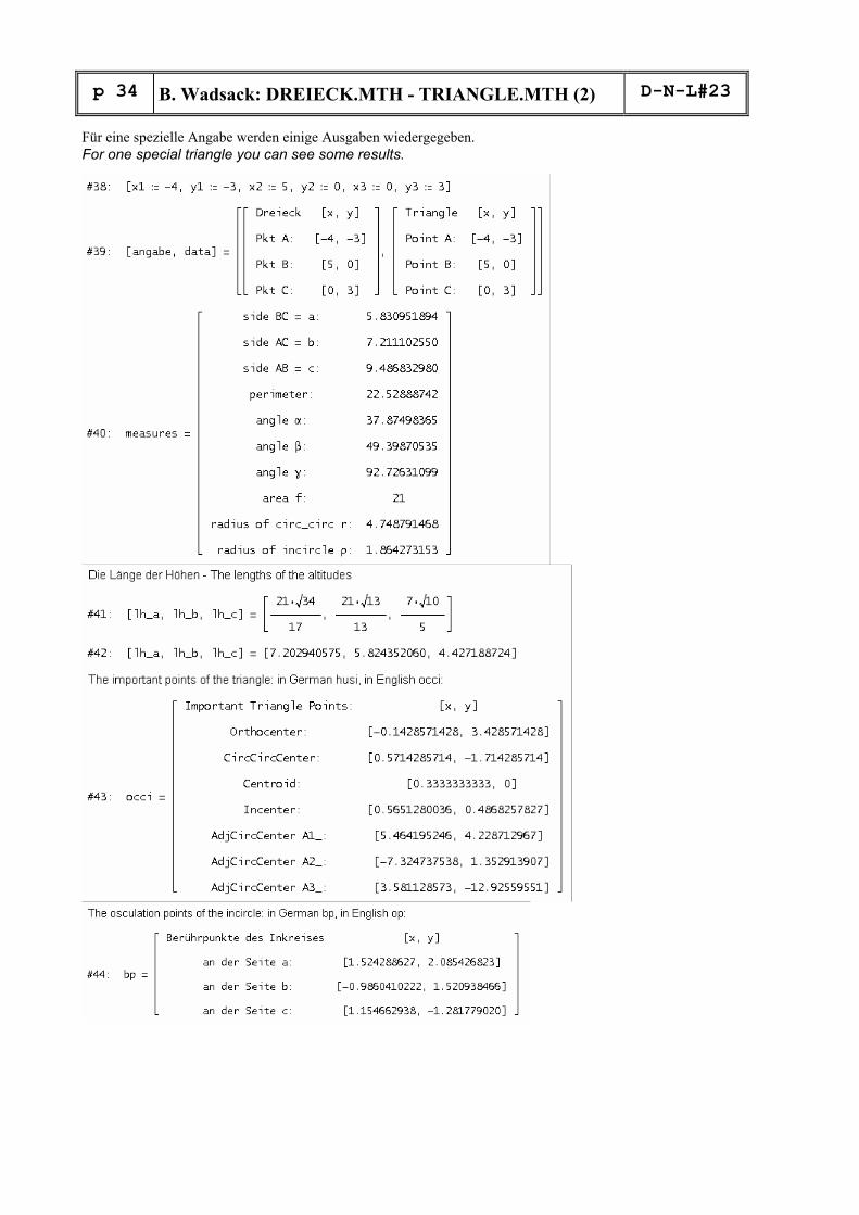
Für eine spezielle Angabe werden einige Ausgaben wiedergegeben. For one special triangle you can see some results.

D-N-L#23


p 35

eckpunkte vertices dreieck triangle angabe data winkel angles l_seiten l_sides Seitenlängen, Lengths of sides abmessungen measures bp op Inkreisberührpunkte, oscpts of incircle fusspunkte pedpoints Höhenfußpkte, pedalpoints of altitudes seiten sides Seiten, sides 0 ≤ p ≤ 1 umkreismpkt circcirccenter Umkreismittelpunkt, circumcenter umkreis circ_circle 0 ≤ p ≤ 2π hoehenschnpkt orthocenter schwerpunkt centroid inkreis incircle 0 ≤ p ≤ 2π inkreismpkt incenter seitsymm perpbisecs 0 ≤ p ≤ 1 winkelsymm angbiss 0 ≤ p ≤ 1 hoehen altitudes -5 ≤ p ≤ 5 schwerlinien medians 0 ≤ p ≤ 1 husi occi alle merkw. Punkte, all interesting points punkte points nur H, U, I, S, only O, C, C, I husilin occilin 0 ≤ p ≤ 1 euler euler eulersche Gerade, Euler line Ankreise adj_circs 0 ≤ p ≤ 2π radien radii

p 36


D-N-L#23

Working sequence for the teaching unit

The remarkable points in the triangle using the utility file DREIECK.MTH

Turn on your computer and start the CAS DERIVE as usual.

Load DREIECK.MTH as an utility file. You will not see the expressions on the screen but they are available for further usage. (Principle of a Black-Box!)

Transfer Load Utility DREIECK ·

Read carefully the instruction how to use DREIECK.MTH (3 pages)!

The following triangle shall be calculated and then be plotted using DERIVE: ∆ABC[A(–4|–3), B(5|0), C(0|3)] Author [x1:= –4,y1:= –3,x2:=5,y2:=0,x3:=0,y3:=3] ·

Now execute the DERIVE calculations. Keep attention to the instruction (page 1 bot-tom and page 2 top). The expressions like angabe, abmessen, ...... husilin have to be edited in the Author line without quotation marks. (That are prepared definitions from the Black-Box!).

Regarding to instruction on page 2 the expressions needed for plotting the triangle like seiten, schwerlinien, .... ,inkreis, ankreise have to be Authored and then Simpli-fied or approXimated. Then you can plot them.

For the 2D-plot use an Overlay window. So the full screen is at your disposal for the construction. In the 2D-plot window set Options Color Auto No ·

Plot the sides in yellow: Options Color Plot 14 · Plot the gravity lines in light red: Options Color Plot 12 ·

Plot the altitudes in light green: Options Color Plot 10 ·

Plot the perpendicular bisectors and the circumcircle in light blue

Plot the angle bisectors, the incircle and the adjacent circles in white!

Important: Save your work as: MY_1WORK.MTH on the diskette! Important: When you are ready with your picture then show it to the teacher!!

D-N-L#23

Carl’s & Marvin’s Laboratory 3

p 37

An Exercise to Motivate Eigenvalues

Carl Leinbach & Marvin Brubaker, USA

In this section we will give a visual demonstration of the effect of applying a 2 by 2 matrix to a simple two dimensional figure. We will see this figure compressed and turned in the direction of the dominant eigenvector of the matrix. Before starting this demonstration, create a Plot window aside of the Algebra window and choose the Connected option for Plotting points. First we create the figure to which we are going to apply our matrix. Enter a 2 by n matrix that gives the coordinates of a house. The first row contains the x-coordinates, the second row the y-coordinates.

h:=[-2,-2,-3,0,0,3,2,2,2,-2;-2,2,1,4,4,1,2,-2,-2,-2]

In order to plot the figure represented by our matrix create a vector of 2 by 2 matrices from the 2 by n matrix. This gives a vector of pairs of points that we can plot. NOTE a↓i↓j is DERIVE's way of de-

noting aij. The down arrow (↓) can be replaced with the phrase SUB. (Or in DERIVE 2.x versions use

the ELEMENT(a,i,j) command).

PMAT(b) ≔ VECTOR([b↓1↓i,b↓1↓(i+1);b↓2↓i,b↓2↓(i + 1)]`,i,DIMENSION(b`)-1)

When we apply PMAT to h from above and plot the result we see:

For the matrix, a, that we will study, generate a random matrix. DERIVE has a random number generator called RANDOM. RANDOM(1) generates numbers between 0 and 1. It is almost certain (but not guaranteed) that the following statement will generate a matrix that has a dominant eigenvalue[1]. Edit

[RANDOM(1),RANDOM(1);RANDOM(1),RANDOM(1)]

(To be sure to obtain different results at any start of the file Edit and Simplify first the expression RANDOM(0)).

p 38


D-N-L#23

Approximate this expression and then assign that result to the matrix, a. Here is one example of ap-proximating the above

Now, we assign this result to the matrix, a. We must do things in this order. Otherwise, the matrix a will change each time it is applied. Use the F3 key to Edit

a ≔ [0.419901, 0.23371; 0.665553, 0.940504]

Let’s see what happens to the house under the action of a.

Clear the plot window and first approXimate Let’s apply a again. then Plot PMAT(a⋅h). Plotting PMAT(a^2⋅h):

Now we apply the 10-th power of a to h. Change the scale in the plot window to x = 0.02, y = 0.02 and Plot PMAT(a^10⋅h):

It is so ´squashed´ it looks like a line. If we apply a to h any more times we will still get this line. It appears to stay fixed under the ac-tion of a. If so, any point on the line will just map onto another point on the line, i.e.

a ⋅ x = δ x

for any point, x, on the line we see on the screen.

Let’s find δ. Move the crosshair to the point with the x-coordinate 0.01. Our reading of this y-coordinate is 0.0312.

D-N-L#23


p 39

Now let’s see what happens to this point under

the action of a. Author a . [[0.01],[0.0312]]

The result is: [0.01149076; 0.03599926]. Dividing the x-coordinate of the above by 0.01 we have an estimate for δ of δ = 1.14907.

We can check this experimental result by finding the roots of the Characteristic Polynomial. If we Simplify CHARPOLY(a), we have:

The largest root of this polynomial is w = 1.15275.

This differs from our experimental result by only 0.00368. Not bad.

Reset the screen and define r as follows:

Repeat the above exercise replacing a with r. Are the results the same? Check out the roots of the Characteristic Polynomial for r.

It is very nice to use the VECTOR command to make visible the effect of ongoing multiplying the ob-ject matrix h by any "random" matrix a or by the "determined" matrix r. Josef

matrix a another random matrix matrix r from above

[1] You can find an exciting application of dominant eigenvectors in DNL#68, page 12

p 40

ERF Functions in DfW4 and DERIVE 6.10

D-N-L#23

ERF functions in DfW4 (and DERIVE 6.10)

Another view from the

DERIVE Window (DfW 4.0) Compare DfW4 and DERIVE 6 (below)!

ERF(x+y)2 + ERF(x⋅y)2

D-N-L#23

DERIVE´s Plotting Accuracy

p 41

Playing with DERIVE´s Plotting Accuracy

Josef Böhm and Charles Reno, Euclid, USA

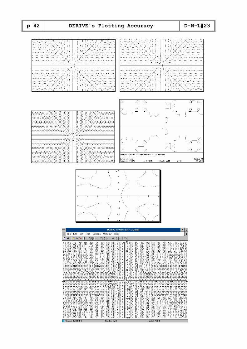
When I attended the T3 Conference in Columbus, Ohio, I met Charles Reno from Euclid, Ohio and during a break he challenged DERIVE to plot the implicit function

x y y xsin( ) cos( )2 2=

Immediately we tried - in the default Accuracy 7. As we were not really satisfied with the result we increased the accuracy up to 9 and then, because the picture needed too much time to be built up we again decreased the accuracy. So we met many different patterns dependent on the plotting accuracy. It was fascinating to observe DERIVE´s plotting algorithm applied on this example.

You can follow the sequence of accuracy in the next screen shots. But one warning: if you have the intention to reproduce the plots then you should preserve a lot of time.

On the next page you can find two plots made by DERIVE for WINDOWS. The plot process in DfW is very much faster than in the DOS version - but it seems that you don’t have any possibility to change the accuracy.

p 42

DERIVE´s Plotting Accuracy

D-N-L#23

D-N-L#23

A C D C T w o

p 43

Solution of the problems from ACDC One

p 44

A C D C T w o

D-N-L#23

D-N-L#23

A C D C T w o

p 45

Another DfW Screen Dump (Dfw 4 )

The graphics are - like the others in this and earlier DSL’s - produced by students of Luk Van den Broeck, Belgium.

See below the pompoen (= pumpkin) and the paddestoel (= mushroom) in DERIVE 6.

p 46

T i t b i t s ( 8 )

D-N-L#23

Titbits from Algebra and Number Theory by Johann Wiesenbauer, Vienna

Hi folks, long time no see! Well, on second thoughts this greeting might be inappropriate in your case as I have just met quite a few of you at the second international DERIVE conference in Bonn this summer. Speaking of Bonn this was really a very special event! As for me it was here that I first got a lot of feedback as regards this column. Boy, modesty forbids me to say more than that I was really flattered! On the other hand I don’t want to cover up the fact that I also met people who were in the bad habit of skipping my column regularly being of the opinion that it is strictly for the birds. You happen to be one of them and were just about to turn over? Phew! Please, read on! I promise to bend over backwards to please you this time! Have you ever regretted the fact that DERIVE has no built-in function to solve even the simplest nonlinear sys-tems of equations? If you agree then the following routine might come in handy: SOLVE2(u,v,x,y):=ITERATE(IF(LHS(l_ SUB 1)=y, APPEND(DELETE_ELEMENT(l_,1),RHS(VECTOR( [x_,l_ SUB 1], x_, LIM( SOLVE(v,x),y,RHS(l_ SUB 1))))),APPEND(DELETE_ELEMENT(l_,1), RHS( VECTOR([l_ SUB 1,y_],y_,LIM(SOLVE(v,y),x,RHS(l_ SUB 1))))), l_), l_,ITERATE(SOLVE(g_,IF( PRODUCT(v_-x,v_, VARIABLES(g_))=0,x,y,y)), g_, ITERATE(RHS(v)*QUOTIENT(u_,LHS(v))+ REMAINDER(u_, LHS(v)),u_,LHS(u)-RHS(u)),1)) Here u and v are two polynomial equations in x and y where v should be the “simpler” of the two equations. It is supposed to work whenever RED(u,v):=ITERATE(RHS(v)*QUOTIENT(u_,LHS(v)) + REMAINDER(u_,LHS(v)),u_,LHS(u)-RHS(u)) (cf. DNL #20) yields a solvable expression in one variable only. Using these functions example 1 from DNL #21, p.39, would now look like this: RED(x^2-x*y-y=113,y^2-x*y+x=-41)=126*(y+13)/(y-1)^2-70 SOLVE2(x^2-x*y-y=113,y^2-x*y+x=-41)=[[15,7],[-61/5,-16/5]]

I used what I call the iterate(...,1)-trick to “combine RED and solve”, as Josef put it in the article quoted above, and it might be of use in other cases as well: SOLVERED(u,v):=ITERATE(SOLVE(u_,VARIABLES(u_)),u_,RED(u,v),1) Actually, it was this preliminary version of SOLVE2 which I distributed to some people at the conference in Bonn. It is still useful in some cases like in my example 2 in the DNL #21, p.39:

P(v):=(a*(b-v)+r*t*v^2)/(v^2*(v-b)) SOLVERED(DIF(P(v),v),DIF(P(v),v,2))=[v=3*b,v=inf,v=-inf] Here SOLVE2 won’t work because of a very nasty bug in the current version 3.14e of DERIVE. Which one? Well, DERIVE commutes sometimes the operations DIF and LIM where this isn’t allowed, e.g. in LIM(DIF(xy,x),y,x)=2x There are other cases where SOLVE2 should work in theory but doesn’t in practice because of a memory over-flow e.g.

SOLVE2(x^2-2*x*y-3*y=1,y^2-3*x*y+2*x=-4) In these cases the modified routine NSOLVE2(u,v,x,y):=ITERATE(IF(LHS(l_ SUB 1)=y,APPEND( DELETE_ELEMENT(l_,1),RHS(VECTOR( APPROX([x_,l_ SUB 1]), x_, LIM(SOLVE(v,x),y,APPROX(RHS(l_ SUB 1)))))),APPEND( DELETE_ELEMENT(l_,1),RHS(VECTOR(APPROX([l_ SUB 1,y_]), y_,LIM(SOLVE(v,y),x,APPROX(RHS( l_ SUB 1)))))),l_),l_, ITERATE(SOLVE(g_,IF(PRODUCT(v_-x,v_,VARIABLES(g_))=0,x,y,y)), g_, ITERATE(RHS(v)*QUOTIENT(u_,LHS(v))+REMAINDER(u_,LHS(v)),u_,LHS(u)-RHS(u)),1)) should give you at least approximate solutions (n stands for numeric!). Unlike the usual numeric procedures you will get all the solutions (even complex ones if any!):

NSOLVE2(x^2-2*x*y-3*y=1,y^2-3*x*y+2*x=-4)= [[3.58397,1.1649],[-1.68707,-4.93439],[-1.04845-0.353058*#i,-0.415254+ 0.495038*#i],[-1.04845+0.353058*#i,-0.415254-0.495038*#i]] (440 sec. on a 486DX2/66; 575 sec. on a 486/33; 110 sec. on a Pentium)

D-N-L#23

T i t b i t s ( 8 )

p 47

You might have noticed that I have always omitted the third and fourth parameter so far. In fact, this is allowed if your variables are x and y which is recommended. If you use other variables than x and y you should make sure that they come before any constants in the order of variables (if necessary use the command “Manage Or-der”) e.g. SOLVE2(a^2+b^2=1,b-r/s*a=-1,a,b) = [[0,-1],[2*r*s/(r^2+s^2),(r^2-s^2)/(r^2+s^2)]]

It is not easy to give general rules when SOLVE2(u,v,x,y) is applicable and therefore it is up to you to experiment a little. Even so, the following two cases deserve to be mentioned: • SOLVE2(p(x,y),ax+by=c), where p(x,y) is a polynomial of degree at most 4 and a,b,c are real numbers. (In

the case a=0 reverse the order of x,y by means of “Manage Order”!) In particular you could use SOLVE2(p(x,y),x=c) or SOLVE2(p(x,y),y=c,y,x), respectively, to calculate points on the curve which is im-plicitly given by p(x,y)=0.

• When dealing with two conic sections try to arrive at SOLVE2(ax^2+bxy+cy^2+dx+ey+f,gy^2+hx+iy+j) with h≠0 or alternatively at SOLVE2(ax^2+bxy+cy^2+dx+ey+f,gx^2+hx+iy+j,y,x) with i≠0 (again reverse the order of x,y in the latter case!) In “school examples” this special form of v can be virtually always achieved by forming suitable linear expressions of the original equations u and v. Since SOLVE2 might take quite long in these cases (or even lead to a memory overflow) you should always try SOLVERED or NSOLVE2 first!

Let me use the remaining space to deal with another “most missing” feature of DERIVE which is sorting a given list of real numbers. Those lists occur in mathematics on many occasions. One example that immediately comes to my mind are the Farey numbers of order n for a given natural number n, i.e. the positive fractions not greater than 1 with a denominator at most n ordered by their size. Assuming that a routine SORT(v) is already available the definition of FAREY(n) could look like this:

FAREY(n):=SORT((ITERATE(IF(a_=b_ AND b_=n,[a_,b_,c_], [IF(a_=b_,1,a_+1), IF(a_=b_,b_+1,b_),IF(GCD(a_,b_)=1, APPEND(c_,[a_/b_]),c_)]),[a_,b_,c_],[1,1,[]])) SUB 3)

As for SORT we could take in this case

SORT(v):=REVERSE_VECTOR(LIM(TERMS(v*VECTOR(x^k_,k_,v)),x,1))

Actually this is nothing else but the sort-routine from my “Titbits(7)” which I believed only sorted different nonnegative integers but which can be taken for different rational numbers as well! Nevertheless I will keep my promise and give you the definition of a sort-routine that sorts arbitrary real numbers:

SORT(v):=REVERSE_VECTOR(LIM(TERMS(EXPAND(VECTOR(k_*x_^APPROX(k_),k_,v)*VECTOR( y_^k_,k_,DIMENSION(v)))), [x_,y_],[1,1]))

(It goes without saying that in both cases the corresponding definition for DSORT(v), which sorts in descending order, is the same but without applying REVERSE_VECTOR.) It works as the following example shows:

SORT([pi,SQRT(3),SQRT(2),#e,SQRT(5),SQRT(2),#e])= [SQRT(2),SQRT(2),SQRT(3),SQRT(5),#e,#e,pi]

I hear you saying that there has already been published such a function in the DNL #22,p.40, by Sergey Biryukov. Ah, I would have liked to dodge that issue because it forces me to admit that I felt totally at a loss when I studied Sergey’s solution. But remembering a story dealing with Alexander the Great when he was in a quite similar situation I cut Sergey’s implementation into two halves throwing away one of them and making some changes to the other. Here is the outcome of my doing:

SSORT_AUX(v,n,p):=VECTOR(IF(MOD(i+p,2)=0,IF(i=1 OR v SUB (i-1)<= v SUB i,v SUBi,v SUB (i-1)),IF(i=n OR v SUB i<=v SUB (i+1), v SUB i,v SUB (i+1))),i,n)

SSORT(v):=ITERATE(SSORT_AUX(SSORT_AUX(w,DIMENSION(v),0),DIMENSION(v),1),w,v)

Just one small example to give you an impression of the calculation times: For n=50 there are 774 Farey frac-tions to sort. It took 7 sec to calculate them and 1.1 to sort them with the first sort-routine, 1.5 sec with the sec-ond one and 901.4 sec by means of SSORT(v).

p 48

T i t b i t s ( 8 )

D-N-L#23

I should also note that I am currently using a Pentium PC with 166 MHz and 32 MB Ram. It’s really a powerful machine! I used it to calculate the number parts(1840926)=245...373 (1505 digits!) in 12 h 43 min which has been proven to be prime by Morain quite recently . It took DERIVE another 394.3 sec to confirm this. See you next time!(?)

On the diskette Johann gave the solution of the example from DNL#21 using his SOLVE2 routine: ┌ │ 2 2 2 │ #19: SOLVE2(a + b + c = 9, a + b + c = 3, a, b) = │ │ │ └ √3·√(c - 3)·√(-c - 1) + c - 3 √(c - 3)·(√3·√(-c - 1) - √(c - 3)) ┐ - ─────────────────────────────── ──────────────────────────────────── │ 2 2 │ │ √3·√(c - 3)·√(-c - 1) - c + 3 √3·√(c - 3)·√(-c - 1) + c - 3 │ ─────────────────────────────── - ─────────────────────────────── │ 2 2 ┘ √3·√(c - 3)·√(-c - 1) + c - 3 #20: a := - ─────────────────────────────── User 2 √(c - 3)·(√3·√(-c - 1) - √(c - 3)) #21: b := ──────────────────────────────────── User 2 3 3 3 3 2 #22: a + b + c - 24 = 3·(c - 3·c + 1) User=Simp(User) 3 3 3 ┌ ┌ π ┐ ┌ π ┐ #23: SOLVE(a + b + c = 24, c) = │c = 1 - 2·SIN│────│, c = 2·COS│───│ + 1, c = └ └ 18 ┘ └ 9 ┘ ┌ 2·π ┐┐ 1 - 2·COS│─────││ └ 9 ┘┘ #24: "The following equation together with a^3+2b^3=24 shows that" User #25: "no two variables, like e.g. b and c, may have the same value:" User 2 2 ┌ 3 0 ┐ #26: SOLVE2(a + 2·b = 9, a + 2·b = 3, a, b) = │ │ User=Simp(User) └ -1 2 ┘ #27: "Therefore apart from permutations this is the unique solution:" User ┌ ┌ π ┐ ┌ π ┐ ┌ 2·π ┐┐ #28: │a := 1 - 2·SIN│────│, b := 2·COS│───│ + 1, c := 1 - 2·COS│─────││User └ └ 18 ┘ └ 9 ┘ └ 9 ┘┘ #29: "Let's check all the terms in question:" User #30: Trigonometry := Collect User ┌ 2 2 2 3 3 3 4 4 4┐ #31: └a + b + c, a + b + c , a + b + c , a + b + c ┘ User ┌ ┌ π ┐ ┌ π ┐ ┌ π ┐ ┐ #32: │3, 4·COS│───│ - 2·√3·COS│────│ - 2·SIN│────│ + 9, 24, 69│ Simp(#31) └ └ 9 ┘ └ 18 ┘ └ 18 ┘ ┘ #33: "DERIVE can't cope with a^2+b^2+c^2 but by approximating we arrive at" #34: [3, 9, 24, 69] Approx(#31)

D-N-L#23

The TI-92 Corner

p 49

THE TI-92 CORNER (EDITED BY B. WAITS, F. DEMANA, B. KUTZLER & J. BÖHM)

DIRA - A TI-92 PROGRAM FOR DISCUSSING RATIONAL FUNCTIONS BY W. PRÖPPER, NÜRNBERG, GERMANY

When using the TI-92 more often to do the necessary computations for discussing functions one soon sees what a boring activity this is. The same operations have to be done again and again: Enter the term of the function, store it as f(x), let the derivatives be computed and store them with other names, compute zeros of the function and its derivatives and so on. At the end you can get a nice plot. What was more obvious than using the programmability of the TI-92 to pass all the routine works to the calculator. I was inspired to do so by a little contribution by J. Böhm in DNL #15 from Sept. 1994. There a Derive-utility was introduced, in which only the function’s term had to be entered and Derive did the whole discussion. This contribution shows in a comprised form the possibilities of DIRA when discussing rational func-tions. After inputting dira() (ENTER) on the home screen of the TI-92 you see this opening screen:

fig. 1 Looking into the menus an expert foresees which mathematical activities take place in each item. Algebraic investigations with (F3):

fig. 2

Investigations by means of calculus with (F4):

fig. 3

Graphs and tables with (F5):

fig. 4 Tools are found in (F1):

fig. 5 To be able working with DIRA a function’s term must be entered first via (F2):

fig. 6 The DIRA-screen shows the actual function:

fig. 7

p 50

The TI-92 Corner

D-N-L#23

By (F3)(6) all algebra-items are run through:

fig. 8

After that (F4)(1) computes the derivatives:

fig. 9

Extrema and inflection points can be found in one run by calling (F4)(4):

fig. 10

The tangent at inflection points are found with (F4)(5):

fig. 11

Finally the graphs of the function and its first derivative (dotted): (F5)(2) and (3):

fig. 12

The program with a more detailed documentation will be found on the annual DNL-diskette. By means of the TI-Graph Link it can be transferred from the PC to the TI-92. From autumn 1996 you can find it in its most recent version on the home page of my school with the web address http://www.nuernberg.de/ver/schg/nk/.

Many thanks Wolfgang for your wonderful "Christmas gift". Maybe I’ll find a way to put your files in a read- and printable form on the diskette, too. Then our friends who have not GRAPH LINK available can also benefit from your program. See the first lines of DIRA´s HELP subroutine:

() Prgm ClrIO Disp " H e l p s c r e e n (1)" Disp "" Disp "DIRA is a program which does the routine-" Disp "work when DIscussing RAtional functions." Disp "" Disp "In menu [F3] algebraical methods like" Disp "computing domains, zeros, poles and" Disp "asymptotes are applied."

D-N-L#23

The TI-92 Corner

p 51

DETERMINING EQUATIONS OF CONIC SECTIONS BY M. BRUBAKER & C. LEINBACH, USA

Introduction: Given the following figure, find the equation of the circle. Where is its center located? What is its radius?

The strategy is obvious. Use the cursor to digitize some points and use these points to de-termine the equation of the circle. How many points do we need to digitize? The answer be-comes clear if we look at the standard equation for a circle.

( ) ( )x h x k r− + − =2 2 2

There are three unknowns, the x-coordinate of the center, the y-coordinate of the center, and the radius. We can find the equation by obtaining three points that lie on the circle, substitut-ing, and solving the resulting three equations for the unknowns, h, k, and r. This process is straight forward, but, because of the fact that the unknowns appear to the first and second power in the resulting equations, tedious. We propose a different strategy that can be easily extended to find the equations of other conics in standard form. Let’s suppose that (x,y) is a point on the circle, then

( ) ( )x h x k r− + − =2 2 2

which we can expand to

x y h x k y k h r2 2 2 2 22 2 0+ − − + + − =( ) .

This has the general form of the homogeneous equation

A x y B x C y D( ) .2 2 0+ + + + = (1)

Because we are dealing with the equation of a circle, x2 and y2 terms have the same coeffi-cients. Thus, when we substitute for x and y we have a linear system with unknowns A, B, C and D. Have we increased the number of points needed to find the equation? The answer is no. The symbolic capabilities of our CAS will show that this the case. Let’s get specific. The figure depicted at the beginning of our discussion was chosen so that we could easily identify that the points (–1,1), (6,8) and (7,7) lie on the circle. Substi-tuting these points into equation (1) above we have:

p 52

The TI-92 Corner

D-N-L#23

2 0100 6 8 049 7 7 0

A B C DA B C D

A B C D

− + + =+ + + =+ + + =

(2)

This still leaves us short one equation, or does it? We still have equation (1) and our CAS. If we think of (x,y) as a general point on the circle, we have a system of four homogeneous equations in four unknowns. From the theory of equations we know that this system will have a nontrivial solution if and only if the determinant of the coefficient matrix is zero. We enter this matrix using the Matrix editor of the TI-92.

In the following figure we take the determinant of this matrix (which we called conic). Setting this result equal to 0 yields the equation of the circle. Completing the square will reveal cen-ter and radius. To graph the circle, it is best to use polar equations. Once again the CAS makes this easy. We use local substitution with x = r.cos(θ) and y = r.sin(θ) and solve the resulting ex-pression for r (≠0). This generates the graph at the start of this article.

This same idea can be extended to the other conics. The general form for a parabola is

A x B x C y D2 0+ + + = or A y B y C x D2 0+ + + = and for ellipse or hyperbola (depending on the location of the points) is

A x B y C x D y E2 2 0+ + + + = . Locating three points on the graph of a parabola or four on the graph of an ellipse or hyper-bola and entering the appropriate matrix will quickly generate the equation of the conic in question. Locating three points on the graph of a parabola or four on the graph of an ellipse or hyper-bola and entering the appropriate matrix will quickly generate the equation of the conic in question.

THE DERIVE - NEWSLETTER #23 USER GROUP - Austromath

Documents

Transcript of THE DERIVE - NEWSLETTER #23 USER GROUP - Austromath