The Dark Side of Technological Progress? Impact of

E-Commerce on Employees at Brick-and-Mortar

Retailers

Sudheer Chava∗ Alexander Oettl∗† Manpreet Singh∗

Linghang Zeng∗‡

First Draft: October 11, 2017

Current Draft: June 2, 2018

∗Scheller College of Business, Georgia Institute of Technology†National Bureau of Economic Research‡Sudheer Chava can be reached at sudheer.chava@scheller.gatech.edu. Alexander

Oettl can be reached at alex.oettl@scheller.gatech.edu. Manpreet Singh can bereached at manpreet.singh@scheller.gatech.edu. Linghang Zeng can be reached atlinghang.zeng@scheller.gatech.edu. We thank Rohan Ganduri, Xavier Giroud, Inessa Liskovich(discussant), Nikhil Paradkar, Daniel Paravisini, Hoonsuk Park (discussant), seminar participants atGeorgia Tech, University of Toronto, Wilfrid Laurier University, ABFER Annual Conference, and MFAAnnual Meeting for comments that helped to improve the paper. We gratefully acknowledge fundingsupport from the Kauffman Foundation Junior Faculty Fellowship. The views expressed in the paperare our own and do not represent the views of the credit bureau and other data providers.

Abstract

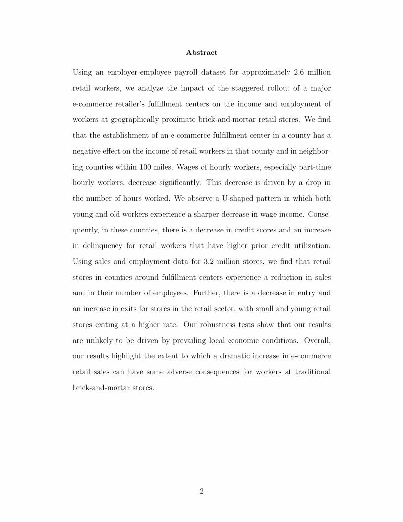
Using an employer-employee payroll dataset for approximately 2.6 million

retail workers, we analyze the impact of the staggered rollout of a major

e-commerce retailer’s fulfillment centers on the income and employment of

workers at geographically proximate brick-and-mortar retail stores. We find

that the establishment of an e-commerce fulfillment center in a county has a

negative effect on the income of retail workers in that county and in neighbor-

ing counties within 100 miles. Wages of hourly workers, especially part-time

hourly workers, decrease significantly. This decrease is driven by a drop in

the number of hours worked. We observe a U-shaped pattern in which both

young and old workers experience a sharper decrease in wage income. Conse-

quently, in these counties, there is a decrease in credit scores and an increase

in delinquency for retail workers that have higher prior credit utilization.

Using sales and employment data for 3.2 million stores, we find that retail

stores in counties around fulfillment centers experience a reduction in sales

and in their number of employees. Further, there is a decrease in entry and

an increase in exits for stores in the retail sector, with small and young retail

stores exiting at a higher rate. Our robustness tests show that our results

are unlikely to be driven by prevailing local economic conditions. Overall,

our results highlight the extent to which a dramatic increase in e-commerce

retail sales can have some adverse consequences for workers at traditional

brick-and-mortar stores.

2

I. Introduction

Technological advances can create enormous economic benefits for society. But, tech-

nological progress and automation can also reshape and transform some labor markets.

They can change the way some tasks are conducted, and these changes can augment

the productivity of some workers but replace other workers entirely.1 In this paper, we

study the impact of e-commerce, which is one manifestation of technological advances in

the retail sector. In particular, we study the effect of e-commerce on the employees of

traditional brick-and-mortar retail stores.

The retail sector is a major employer in the U.S., employing approximately 16 million

workers, or 13% of private sector employment, at the end of 2016 (Bureau of Labor Statis-

tics). The retail industry landscape has changed dramatically in the last few decades. In

the earlier decades, the disruption was mainly driven by the expansion of major retail

chains such as Walmart and by the rise of discount retailers (Jia (2008), Holmes (2011),

Basker (2005), Neumark et al. (2008)). But, the recent disruption in the retail sector is

attributed to the rise of technology led by e-commerce. It is projected to result in the

shuttering of more than 8,000 retail stores by the end of 2017.2 So, the retail sector is

an economically important setting for studying the impact of technological progress, as

represented by e-commerce, on the labor force in the traditional retail sector.

Identifying the causal impact of e-commerce on the employees of traditional brick-

and-mortar retailers is challenging, since we cannot observe the counterfactual, i.e., what

would the income and employment of brick-and-mortar retailer employees be in the ab-

sence of e-commerce? We address this identification concern by using the staggered roll-

out of the fulfillment centers (FCs) of a major e-commerce retailer. We use this rollout

1See National Academy of Sciences Report on Automation (2017); Acemoglu (2002); Autor, Levy, andMurnane (2003); Brynjolfsson and McAfee (2011 and 2014); Autor (2015); Autor, Dorn, and Hanson(2015).

2See https://on.wsj.com/2poCwtG. Further, some online retailers have highly automated warehousesthat use robots to bring items for a retail order from their storage shelves. The world’s largest e-commerce retailer employed 45, 000 robots in its fulfillment centers, a 50% increase from previous yearsholiday season. https://bit.ly/2EldAGf

1

as a proxy for the presence of local e-commerce and a large administrative employer-

employee payroll dataset with detailed data on income and employment from a major

credit bureau. Although the e-commerce retailer has FCs across the country, the timing

of the establishment of FCs was staggered across the U.S. from 1997 to 2016. Our em-

pirical strategy estimates the causal impact of the establishment of a new FC by a major

e-commerce retailer on the income and employment of retailer workers in that county

and in neighboring counties.

We use a large administrative employer-employee payroll dataset from a major credit

bureau. This dataset contains detailed data on income and employment. We restrict the

sample to 57 major retail firms that employ a total of approximately 2.6 million retail

workers. This comprises 18% of total U.S. retail employment in the first quarter of 2010.

Our rich payroll information allows us to group workers into hourly workers and non-

hourly workers (referred to as salaried workers). These data include total compensation,

wage/salary, overtime, bonuses, commissions, and wage/salary rate. We analyze this

matched employer-employee dataset, and we use a difference-in-differences setting to

exploit the staggered introduction of the FCs. We find that the labor income of retail

workers in counties with FCs, on average, decreases by 2.4% after the establishment of

FCs. This negative effect is also significant for workers within 50 or 100 miles of FCs.

These results are confined to hourly workers, who experience a decrease in labor income

by 2.5%, which is equivalent to an $825 decrease in annual income. Most of the effect

derives from a reduction in the number of hours worked. Among hourly workers, we find

a particularly strong negative impact on part-time hourly workers. Further, we observe

a U-shaped pattern in which both young and old workers experience a sharper drop in

labor income.

One potential concern about our identification strategy and our results may be: Why

do the e-commerce retailer’s FCs matter for traditional brick-and-mortar store sales? At

the beginning of 2000, the e-commerce retailer had only three FCs, but the staggered

2

introduction of FCs across different counties resulted in the retailer having more than

90 FCs by the end of 2016 (Figure 1 and Figure 2). Optimizing and expanding the

FC network is an important strategy used by the e-commerce retailer to meet customer

demand and save costs. The establishment of FCs allows the e-commerce retailer to

optimize and distribute their inventory placement (even for third party sellers). This in

turn allows the e-commerce retailer to reduce its shipping costs and shipping times. The

e-commerce retailer can offer same-day or 2-day shipping for a longer time during the

shopping day from the nearby FCs, making a purchase from the online retailer attractive

relative to the traditional brick-and-mortar stores in the vicinity.

Moreover, the e-commerce retailer does not collect local sales taxes and has only

recently begun to collect state sales tax on sales from its inventory (Baugh, Ben-David,

and Park (2018)). However, it does not yet collect state sales tax from most of its third

party sellers (that account for more than 60% of the retailer’s sales). This could lead

to a price advantage over the traditional retailers. Also, the establishment of an FC is

meant to avoid long-zone shipping. Therefore, the establishment of an FC is likely to

have a more significant effect on geographically nearby areas, a fact that we exploit in

our identification strategy.

Consistent with aforementioned arguments, we find that the establishment of the

e-commerce retailer’s FCs impact the sales of geographically proximate traditional brick-

and-mortar retail stores. Using sales data from the National Establishment Time Series

(NETS), we find that after the establishment of the e-commerce retailer’s FC, the annual

sales of stores decrease by $63,639 per store, i.e., 2.8% of the total annual sales of the

average store in our sample. We find that the annual sales of stores in the top tercile,

based on sales one year before the FC, decrease by $200,389.

A second potential concern regarding our identification strategy and our results is

that the decision of establishing an FC in a county is probably not random. The decision

may in fact be correlated with local economic conditions. As the goal is to better serve

3

customers in surrounding areas, FCs are more likely to be built close to, or in, areas with

high retail sales and population density. Our fixed effect methodology can control for

these level differences. However, it is possible that the e-commerce retailer may choose to

locate its FCs in areas with decreasing competition from brick-and-mortar retail stores,

i.e., areas where the retail sales of brick-and-mortar stores are declining.

We formally test this hypothesis using differences in the demographics and retail sales

data computed from 2000 and 2010 county-level census data. We find that the change in

population density is the only change that is significantly and positively related to an FC

establishment, while growth in the unemployment rate, median household income, and

age distribution do not correlate with the location choice of FCs. Further, the positive

coefficient on retail sales growth gives us confidence that our estimation may not be driven

by a downward trend in the traditional retail sector. We also find a lack of pre-trends

before the establishment of the FCs, lending credence to our identification strategy.

The inclusion of state-year-quarter fixed effects mitigates potential concerns about

unobservable local economic conditions being the driver of our results. We further add

more granular county-year-quarter fixed effects to control for local economic conditions

by using the data available for workers of non-retail firms as a control group. Moreover,

the opening of FCs has no impact on the sales of full-service restaurants in the county,

supporting the view that the impact is due to the establishment of the FCs and not due

to negative local economic conditions.

Another potential concern is that there may be an omitted firm-specific shock to the

traditional retailers that is contemporaneous with the establishment of the e-commerce

retailer’s FC in that county. For example, some firms may have concentrated operations

in certain areas, and they may face firm-specific negative shocks (e.g., the failure of a

major lender, the bankruptcy of a supplying firm) at the same time the e-commerce

retailer builds an FC in that county. To address this concern, we include firm×year-

quarter fixed effects in our regressions. Our results are robust to the inclusion of these

4

fixed effects.

As we argued before, the establishment of FCs can cut shipping costs and shipping

time. It is possible that this may induce some consumers to purchase from the online re-

tailer instead of brick-and-mortar stores. It is likely that some of these benefits disappear

as consumers become more and more distant from the FCs, thue reducing the impact on

traditional retail stores and consequently on the workers at these stores. On the other

hand, for counties with FCs or counties are geographically close to the FCs, any positive

labor demand due to hiring by the FCs may reduce the direct negative impact on the

traditional stores. In line with these arguments, we find that the income effect is -1.9%

for counties with FCs, and it is strongest (-3.9%) in counties within 50 miles of FCs. This

effect monotonically decreases over the distance after 50 miles. It becomes insignificant

for counties within 500 miles of FCs.

As a reaction to the increased competition from the e-commerce retailer, the affected

stores may focus on customer service and rely more on employees. On the other hand,

facing lower sales, affected stores may not only cut wages but also adjust their overall

employment level. We find that for all stores, employment decreases by 2.4%, which is

equivalent to 41 fewer workers per 100 stores for a store with an average of 22 employees.

We find that, for large stores, employment decreases by 1 worker per store for a store

with an average of 40 employees.

Finally, using NETS data, we analyze store closures and new store openings. We find

that the exit rate increases by almost 3%. The average exit rate in our sample is 13.6%.

Small stores are more likely to exit than large stores. More interestingly, young stores

are more likely to close. We also find that after the establishment of FCs in a county,

the entry rate for small stores reduces significantly by 11.8%. This low entry rate effect

is not just limited to counties with FCs; it also exists for counties in 50 or 100 miles of

FCs.

Our paper directly relates to the literature that documents the effect of technological

5

changes on labor market (Krueger (1993); Autor, Katz, and Krueger (1998); Acemoglu

(2002); Autor, Levy, and Murnane (2003); Autor (2015); Autor, Dorn, and Hanson

(2015)). Further, we add to the literature on the income and employment effect of

competition. This issue has been studied in the context of the expansion of large chain

stores (Basker (2005); Neumark, Zhang, and Ciccarella (2008)) and import competition

(Autor, Dorn, and Hanson (2013); Autor, Dorn, Hanson, and Song (2014)). The rise of

e-commerce is one of the most important technological changes in the retail sector, and

it may create competition for brick-and-mortar retail stores. We use the establishment of

a major e-commerce retailer’s FCs as a proxy for the increase in local competition, and

we test the effect of this competition on the income and employment of retail workers.

Our paper also relates to research on the causes and consequences of disruption in the

retail sector. Existing research focuses on the disruption that results from the rollout of

large chains. Holmes (2011) estimates the benefits and costs for the rollout of Walmart

store openings. Jia (2008) quantifies the effect of the expansion of retail chain stores on

other retailers. Basker (2005) and Neumark, Zhang, and Ciccarella (2008) estimate the

employment and earnings effect as a result of Walmart store openings. We investigate

the disruption attributed to e-commerce.

Our research contributes to the literature on the impact of e-commerce. Compared to

brick-and-mortar retailers, e-commerce provides consumers a lower price (Brynjolfsson

and Smith (2000)), and increased product variety (Brynjolfsson, Hu, and Smith (2003);

Ghose, Smith, and Teland (2006)). The introduction of e-commerce by a firm increases

its market value and revenue (Subramani and Walden (2001); Pozzi (2013)). While these

above papers examine the impact of e-commerce on consumers and firms that adopt

e-commerce, we analyze the labor market consequence of a major e-commerce retailer’s

expansion of its FC network.

One important caveat with our result is that, given the scope of our paper and empir-

ical strategy, we are limited to documenting one facet of the impact of the technological

6

innovation in the retail sector. There are many positive benefits of e-commerce for con-

sumers, including potentially lower prices, more choices, convenience in shopping, gains

from competition, and lower effort (e.g., no driving). Moreover, the establishment of the

FC may have positive spillovers in the local community and could increase employment.

However, the scope of our paper is limited; it focuses only on the impact on the workers

in the geographically proximate traditional retail stores.

If there are no frictions in the labor market (i.e., workers can easily switch jobs

and their skills are completely transferable) then the short-term displacement of some

traditional retail store workers that we document may not matter for the workers or the

local economy. However, in the presence of frictions in the labor market, the short-term

impact on the workers and local economy can be negative. Moreover, to the extent that

the scope of work differs between traditional retail stores and warehouses, at least some

workers can be worse off. For example, there is no need for cashiers at an FC, and skills

may not be completely transferable between traditional retail stores and e-commerce

FCs.

In the long run, some of the affected workers may find alternate employment in their

same field, or they may acquire new skills to find employment in another field. This would

result in workers being better off after the establishment of an FC. Again, the scope of

our paper is limited, and we focus only the short-term impact of the establishment of

the FCs of the e-commerce retailer. Our results highlight one negative consequence of

technological progress in the retail sector: the short-term negative impact on the wages

and employment of some traditional brick-and-mortar retail store employees.

The rest of the paper proceeds as follows. We discuss our empirical methodology and

identification threats in Section II. In Section III, we describe the various sources for the

data used in the analysis and provide summary statistics. Our main empirical results are

presented in Section IV. We conclude in Section V.

7

II. Empirical Design and Identification Challenges

A. Empirical Design

In this study, we seek to examine the impact of technological progress, in the form

of the expansion of e-commerce, on traditional brick-and-mortal retail establishments

and their workers. In order to isolate the effects of the establishment of FCs from other

regional, sectoral, and macro-level shocks, we exploit the staggered rollout of FCs to

capture the increase in the presence of local e-commerce. While the location that the

major e-commerce retailer chooses for its FCs is certainly not random, we present evi-

dence demonstrating that the timing of an FC establishment is plausibly exogenous to

unobserved factors that may impact local retail establishment performance. Specifically,

our empirical strategy estimates the impact of the establishment of an FC in a county

on retail workers in the same county and in neighboring counties.3

Why do FCs matter? First, the optimization and expansion of the FC network is

important to the e-commerce retailer to meet customer demand and reduce costs. The

e-commerce retailer built its first FC in 1997, and the number of FCs increased to over

90 by the end of 2016 (Figure 1 and Figure 2). Second, the establishment of a new FC is

meant to avoid long-zone shipping. The FC is established to reduce the costs associated

with shipping as well as the time required for customers to receive their packages.

Furthermore, it is evident that FCs are primarily located on the east and west coasts,

where population density is highest.4 Third, as discussed in Houde, Newberry, and

Seim (2017); customers may value the convenience effect due to faster delivery, so that

the establishment of an FC would induce customers nearby to be more willing to shop

3A complete list of fulfillment centers of the e-commerce retailer is available at http://www.mwpvl.com/.4The 2016 annual report of the e-commerce retailer states “If we do not adequately predict customerdemand or otherwise optimize and operate our fulfillment network and data centers successfully, itcould result in excess or insufficient fulfillment or data center capacity, or result in increased costs,impairment charges, or both, or harm our business in other ways.”...“In addition, a failure to optimizeinventory in our fulfillment network will increase our net shipping cost by requiring long-zone or partialshipments.”. New FCs would be close to large cities, allowing for the possibility of next-day or same-daydelivery and the wider rollout of its grocery business (Stone(2013)).

8

through the major e-commerce retailer rather than shop at a local brick-and-mortar

store. As mentioned before, there may be lower prices for consumers, as the e-commerce

retailer does not collect state taxes for sales by third party vendors on its platform, which

represents approximately 60% of its sales.

Furthermore, the e-commerce retailer does not collect local sales taxes, if any tax at

all, for most of its customers. E-commerce retailing in principal allows for the ability to

serve all potential customers on a national scale. However, in practice, the establishment

of an FC will have a larger effect on areas surrounding the FC. As such, this increase

in the value to local consumers of shopping from the major e-commerce retailer may

negatively affect the income and employment of workers in brick-and-mortar stores.

Our empirical objective is to evaluate the local effect of the establishment of a new

FC.5 We do so by focusing on three definitions of local : 1) the focal county (i.e., the

county where the FC opened) 2) all counties within 50 miles of the FC (excluding the

focal county where the FC is located) and 3) all counties within 100 miles of the FC

(again excluding the focal county where the FC is located).

We treat each county as treated in the first quartert in which an FC opens in one of

the three definitions of a local county. For example, for the analysis that focuses on the

focal county level, the indicator for Fulton County, GA, turns on in the first quarter of

2015 since an FC was opened in Union City, GA, (Fulton County) in February of 2015.

In our 50-mile analysis, Cobb County, GA, (a county that abuts Fulton County, GA) is

treated in the first quarter of 2015 from the opening of the same FC in Union City, GA.

Yet, in our 100-mile level analysis, Cobb County, GA, is treated in the third quarter of

2011 due to the opening of an FC in Hamilton County, TN, in September of 2011. As

our data start in 2010, our study focuses on the 39 FCs established after 2010.6

A standard approach for evaluating the impact of the opening of an FC would be

5We follow Houde, Newberry, and Seim (2017) and remove FCs that are established in a county with anexisting FC or within about 20 miles of an existing FC, which reduces our sample to 50 FCs.

6Our results remain robust to the inclusion of all 50 FCs (which includes FCs established before 2010)and is reported in Table IX.

9

to compare differences in brick-and-mortar establishment performance before and af-

ter the FC opening in treated and in untreated counties. However, for this difference-

in-differences specification, we assume parallel trends between the treated and control

counties. However, Table A1 indicates that focal and surrounding counties where FCs

open are very different not only in levels but also in trends from the rest of the U.S.

in terms of demographics and local economic variables, such as population, population

density, retail sales, retail sales per capita, household income, and unemployment rate.

Therefore, these untreated counties may bias our results. Consequently, we only include

counties that were classified as treated at any time by the opening of an FC in our anal-

ysis, and we exploit the variation in the timing of the establishment of FCs, using FCs

that will be treated but are not yet as de facto controls.

In our baseline analysis, we apply a difference-in-differences estimation to quantify

the impact of the establishment of an FC on the income of workers in brick-and-mortar

stores, and we estimate the following:

ln(Total Incomei,c,t) = α + βPostFCc,t + ηi + θt + εi,c,t, (1)

where each quarterly observation is the income of worker i working in county c at time t.

PostFC is an indicator that equals 1 in the quarter an FC is established in county c or

within 50 or 100 miles of county c, and it remains 1 for all subsequent quarters. Time-

invariant worker-specific characteristics and year-quarter shocks are controlled for with

the inclusion of worker (ηi) and year-quarter (θt) fixed effects, respectively. Standard

errors are clustered at the county level. The variable β estimates the percentage change

in income attributed to the establishment of an FC.

B. Identification Challenges

In order for β from Equation 1 to represent an unbiased estimate of the impact of the

establishment on an FC on the income of local brick-and-mortar retail workers, we must

10

assume that PostFC is orthogonal to any unobservables. Yet, because the location of FCs

is not randomly decided by the major e-commerce retailer, dealing with this endogenous

selection represents our main econometric challenge.

A primary concern in our analysis is that the decision to establish an FC in a specific

county will naturally be a function of local economic conditions. Since one of the primary

objectives of establishing FCs is to improve the ability to serve local customers, FCs may

be more likely to be built in areas with high retail sales and high population density. To

test this, on a cross-section consisting of all counties in the U.S., we regress the likelihood

of establishing an FC in county c on county-level long differences (between 2000 and

2010) of retail sales, population density, unemployment rate, household income, and the

percentage of the population between the ages of 18 and 65 (Table II).

We observe that FCs are more likely to be located in counties with faster growing

population densities; but, importantly, not those that have experienced more growth

in retail sales. While our county-level fixed effects will absorb all time-invariant level

effects of county-specific characteristics, our estimated will be biased downward insofar

as counties that experience high population density increases are also more likely to

engage in e-commerce transactions that substitute for local retail purchases. However,

if this scenario were true, we could also observe downward trends in retail sales in the

periods before the FC’s establishment, which we do not (Figure 3).

A second concern surrounds the ability for the major e-commerce retailer to negotiate

with the state and local government about the location of the FC in exchange for tax

benefits or other incentives. It is plausible that governments may want the FC to be built

in an area with weak economic conditions to boost the local employment and economy. As

a result, FC county selection may be negatively correlated with local economic conditions;

and, in particular, negatively correlated with the economic fortunes of brick-and-mortar

retail stores, thus potentially biasing our estimates downward.

However, as shown in Table II, Columns (3) and (4), the establishment of an FC does

11

not relate to the ex ante change in the local unemployment rate and median household

income, which lessens this concern. Furthermore, we deepen our analysis by conducting

a placebo test on sales in another non-tradeable sector: full-service restaurants. As

reported in Section IV.B.5, we do not find any effect on their sales with the establishment

of FCs in the local area.

The e-commerce retailer may also consider the tax implications of an FC. The estab-

lishment of an FC means establishing a physical presence. Though it is not necessary,

the major e-commerce retailer must collect sales tax in some states. Even if this is true,

it is biased against finding any negative impact on nearby traditional retail stores. More-

over, the tax consideration is important in early years. After building FCs in low-tax

states, and given the fact that they have collected sales tax in many states, being closer

to a large market dominates the tax consideration (Stone (2013); Houde, Newberry, and

Seim (2017)). We control for any state-level time-varying unobservables, such as tax

incentives, using state-year-quarter fixed effects.

Last, we may be concerned that the arrival of an FC in a county changes the com-

position of firms. In this case, higher performing firms or firms with greater options in

managing their geographically varied portfolio of stores choose to exit those counties. Or

conversely, the best performing retailers choose not to enter the treated counties. This

would lead to the appearance of a drop in retail performance, but this would be entirely

attributable to a compositional effect whereby the firm-quality distribution experiences

a leftward shift. To deal with this, we focus solely on the intensive margin of competition

by including only firms that are present before and after the arrival of an FC. In addition,

we include establishment-level fixed effects to control for establishment quality.

In summary, it is difficult to establish a convincing causal relation; however, our

confidence in interpreting our PostFC coefficient as causal is increased by the inclusion

of fine-grained establishment, worker, industry-year, state-year, and year-quarter fixed

effects. Our confidence is also increased by the ability to rule out reverse causality or

12

selection on trends, as seen in the lack of any discernible pre-trends in our regression and

in our full-service placebo test.

III. Data

Our empirical analysis makes use of data at three levels of analysis: 1) individual

worker-level data that we obtain from a major credit bureau, 2) establishment-level data

that we obtain from the National Establishments Time Series Database, and 3) county-

level data that we obtain from the Bureau of Labor Statistics. We describe each dataset

and its construction in this section.

A. Worker Data

Our novel comprehensive consumer data are provided by a major credit bureau. The

data contain detailed employment information, including company name, 3-digit NAICS,

the date an employee was most recently hired for the current position, an indicator of

whether an employee is presently active, and rich payroll information that includes the

payment structure by which payments are made to the employee, total compensation,

wage/salary, overtime, bonuses, commissions, and wage/salary rate. We group workers

into hourly workers and non-hourly workers (referred to as salaried workers) based on

their payment structure.

We obtain income and employment data of active employees at the end of each quarter

from the retail firms, which consistently supply data from 2010 to 2016.7 The data are

matched to credit files through tokenized Social Security Numbers (SSNs), which provide

demographic information such as the individual’s ZIP code of residence, age, and gender.

We use the workers’ county of residence to determine their location when examining

7We identify firms in 3-digit NAICS industries that are most likely to compete with the major e-commerce retailer’s product catalog. The 3-digit NAICS codes that we classify as retail includes 442(furniture and home furnishing stores), 443 (electronic and appliance stores), 444 (building material andgarden equipment and supplies dealers), 448 (clothing and clothing accessories stores), 451 (sportinggoods, hobby, book, and music stores), 452 (general merchandise stores), and 453 (miscellaneous storeretailers). In robustness tests, we use workers from all non-retail firms as a control group.

13

the impact of the arrival of an FC.8 Our sample consists of all workers employed in the

first quarter of 2010, and the sample follows them until they exit. Our sample is thus

unbalanced and does not allow for worker entry. In addition, we use the workers’ residency

in 2010Q1 to determine their location (county) for all empirical analysis. We drop workers

who have multiple employers at any time during our sample period. If a worker switches

employers during the sample period, we keep our observations for the first job. All dollar

values are converted to December 2016 dollars using the seasonally adjusted consumer

price index for all urban consumers from the Bureau of Labor Statistics.

Our sample contains 2.6 million workers from 57 retail firms, which accounts for 18%

of the 14.42 million total U.S. retail employment in the first quarter of 2010. The median

firm has more than 14,000 workers in the sample, which suggests that we cover mostly

large firms. Table I, Panel A presents summary statistics for worker-level payroll data.

The mean quarterly income of hourly workers is $7,326. Annualized income is $29,304,

which is slightly higher than the mean income of 8.79 million retail sales workers ($25,250)

and slightly higher than the mean income of 4.53 million retail salespersons ($27,180), as

estimated by the BLS in May 2016. The mean number of hours worked is 30.9 per week,

with an average wage rate of $14.9 per hour. For retail workers in our sample, wage

income contributes to about 87% of their total income. The remaining income derives

from overtime/bonuses/commissions (referred to as a bonus). In our sample, salaried

workers earn $86,016 annually, on average.

The granularity of our worker-level data helps us answer questions that cannot be ad-

dressed solely from aggregate data. Given the fine-grained nature of these data, we can

examine deeper worker-level heterogeneity and analyze which workers are more vulnera-

ble to the establishment of an e-commerce FC. For example, are full-time workers more

affected than part-time workers? Further, does a worker’s gender and age insulate or ex-

8We do not observe the county of the workers’ workplace. However, more than 90% of workers in oursample are hourly workers who are less likely to spend time and money on commuting to work. Whilewe believe that a workers’ residence does an adequate job of proxying for their workplace, we recognizethat this will be measured with some error.

14

acerbate these effects? The detailed composition of the worker’s compensation also allows

us to understand the channels through which workers are affected. Do firms reduce work-

ers wages or bonuses? Do firms cut wage rates or the number of hours worked? Lastly,

these granular data allow us to improve the identification of our regression parameters

through the inclusion of fine-grained fixed effects within a panel regression environment.

B. Establishment Data

In addition to worker-level data, we use establishment-level data for the retail sector

from the National Establishment Time Series (NETS) Database (Walls & Associates,

2014).9 This database provides an annual record for a large part of the U.S. economy

that includes establishment job creation and destruction, sales growth performance, sur-

vivability of business startups, mobility patterns, changes in primary markets, corporate

affiliations that highlight M&A, and historical D&B credit and payment ratings. At the

beginning of our sample year, 2010, the database covers 3,287,183 active establishments

employing 27,404,989 workers with total sales of $2.9 trillion. These data are available

until 2014.

Similar to how we defined retail firms with our worker-level dataset, we select estab-

lishments in 6-digit NAICS industries that are more likely to be affected based on the

e-commerce retailer’s product catalog. Table A2 provides a complete list of industries

selected. To reduce noise from very small retail stores, we keep retail stores with more

than two employees before the establishment of the fulfillment center. Table I, Panel B

reports summary statistics for our sample. It shows that the average retail store in our

sample has annual sales of approximately $1.5 million and 12 employees.

9Walls & Associates converts Dun & Bradstreet (D&B) archival establishment data into a time-seriesdatabase of establishment information.

15

C. County Employment Data

For our county-level analysis, we use publicly available Quarterly Census of Employ-

ment & Wages (QCEW) data provided by the Bureau of Labor Statistics (BLS). This

dataset provides county-level data on employment, wages, and the number of establish-

ments in each 6-digit NAICS industry by quarter. We again select industries that are

likely to be affected, based on the major e-commerce retailer’s product catalog. We use

quarterly data beginning in the first quarter of 2010 and ending in the fourth quarter of

2016. Summary statistics are reported in Table I, Panel C.

IV. Results

In this section, we describe our main empirical results. We first describe our baseline

results using worker-level data. We then describe the robustness tests that we conduct

to rule out competing interpretations of our results and to strengthen the identification

of our parameters. Next, we describe results using NETS establishment data that allow

us to analyze the impact of FC entry on the entry and exit of establishments in the

local retail sector. Finally, we present the impact of FC establishments on the aggregate

county-industry level employment using QCEW data from BLS.

A. How Do FCs Affect Local Brick-and-Mortar Stores? Evidence from Worker-level

Data

A.1. Baseline Results

In Table III, we report the impact of the establishment of FCs on the income of retail

workers in counties with FCs or neighboring counties using the difference-in-differences

specification shown in Equation 1. We include worker fixed effects and year-quarter fixed

effects in all regressions in order to absorb as much variation as possible arising from

worker-specific time-invariant characteristics and temporal trends. Since we define the

arrival of an FC at the county level, we cluster all standard errors at the county level.

16

As shown in Panel A, Column (1), the total income of retail workers in counties with

FCs decreases by 2.4%, on average, after the establishment of an FC. Moving to workers

in counties within 50 or 100 miles of the focal county where an FC was established, we

continue to observe a strong negative effect on total income (Panel B). Since the arrival of

an FC may differentially impact hourly and salaried workers, we run separate regressions

for those two types of workers.

Results in Column (2) show that the income of hourly workers decreases by 2.5%,

equivalent to an $825 cut in annual income. As shown in Column (3), salaried workers

mostly have muted responses to the establishment of FCs. These muted responses may

be attributed partly to the infrequent adjustment of salaries or the inflexibility of firms

in adjusting the incomes of salaried employees in the short term. We focus on hourly

workers thoughout the rest of our analysis, because hourly workers account for more than

90% of our sample and are the ones who experience the largest negative effects.

Our identification strategy, which relies on the staggered temporal rollout (shocks) of

FCs across different counties, assumes that workers in counties that have yet to be treated

by the establishment of an FC serve as an appropriate control group. This assumption

would be violated if FCs are established in counties or regions that are experiencing

upward trends in online shopping and downward trends in sales at traditional brick-

and-mortar retailers. In this case, the negative income effect may be driving the FC

establishment and not vice versa. As such, our difference-in-differences assumption is

only valid if treatment and control groups follow parallel trends before the shock. To test

this, we directly examine the dynamic temporal effects by including leading and lagging

indicators of FC establishment by estimating the following:

Log(Total Incomei,c,t) = α+4∑

j=2

βjPreFCc,t(−j)+4∑

j=0

γjPostFCc,t(j)+ηi+θt+εi,c,t. (2)

To increase the power of our estimates, PreFC and PostFC dummies are defined at half-

17

year intervals. The variable PreFCc,t(-j) (PostFCc,t(j)) is a dummy that takes a value 1

if it is j half-years before (after) the establishment of FCs. Also, PreFC(-4) equals 1 if

it is two or more years before the establishment of FCs, and PostFC (+4) equals 1 if it

is two or more years after the establishment of FCs. The variable PreFC(-1) is dropped

from the estimation so that all coefficient estimates can be treated as percentage changes

relative to the income workers received six months before the establishment of FCs.

In Figure 3, Panel A, we show the dynamic effect of FCs on income for counties with

FCs by plotting the coefficients from the specification in Equation 2. The shaded area

around the coefficients represent 95% confidence intervals. Coefficients on PreFC(-4),

PreFC(-3), and PreFC(-2) are all statistically insignificant from the income of workers

in PreFC(-1) (the omitted category). That suggests that there is no pre-trend in the

data, and our parallel trends assumption appears to be valid. Within six months of the

establishment of an FC, the income of hourly workers decreases by 2.1% relative to the

half-year shortly before the FC’s establishment. The negative effect further increases to

-4.1% two years after the FC’s establishment. We find a similar pattern in Panels B and

C of Figure 3, where we focus our analysis on counties within 50 miles of the county in

which an FC opened and within 100 miles, respectively.

A.2. Can Unobservable Firm-Specific Variables or Local Economic Conditions Be

Driving the Results?

Our results so far suggest a robust and negative relationship between the arrival of

an FC and a worker’s income. However, absent truly exogenous variation in both the

geographic location and temporal timing of FC establishment, we may still be concerned

that the arrival of an FC is correlated with unobservables present in the error term

of Equation 1. These unobservables may include firm-specific characteristics or local

economic conditions that jointly affect both the likelihood of an FC arriving in the county

and the income of workers in local brick-and-mortar establishments.

18

For example, if a major lender or supplier to a brick-and-mortar retailer files for

bankruptcy and this attracts the e-commerce retailer to establish an FC in the county as

a result, then this negative correlation between our error term and the FC establishment

amplifies our negative effect sizes. To address this concern, we include firm-year-quarter

fixed effects to absorb all time-specific characteristics of our sample firms and identify our

parameter of interest by exploiting varition within-firm-time across counties. As such, we

can only estimate our postFC variable from firms that operate in more than one county.

We see in Column (1) that when we include these firm-year-quarter fixed effects, the

establishment of FCs in the county results in lower total income for retail hourly workers

in the brick-and-mortar stores. We find that the magnitude diminishes from the baseline

magnitude (2.5%) to 2.1% for counties with FCs. When we extend our analysis to focus

on counties within 50 and 100 miles of the county in which the FC was established, we

continue to see precisely estimated negative effects.

As discussed in Section II.B, local economic conditions may also play an important

role in the establishment of FCs by the e-commerce retailer. States with and without FCs

may have different economic and regulatory environments, which could correlate with the

establishment of an FC. For example, regions with suppressed economic activity (which

would negatively impact retail sales) may be more inclined to offer sizable incentives

for e-commerce retailers to establish an FC in their region. To control for time-varying

unobservables at the state level, we include state-year-quarter fixed effects and report the

results in Table IV, Column (2). The estimated effect for counties with FCs drops from

-2.5% to -0.8%, but the result remains statistically significant from 0. Further, the results

are strong both economically and statistically for workers within 50 or 100 miles of FCs.

Our results remain robust when we combine firm-year-quarter and state-year-quarter

fixed effects in Column (3).

While the state-year-quarter fixed effects may control for state-level heterogeneity,

they may be insufficient to fully absorb any time-varying heterogeneity that arises at the

19

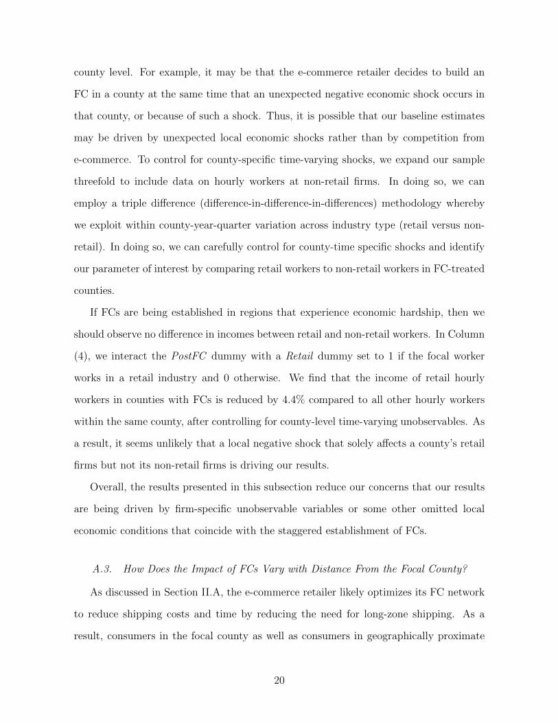
county level. For example, it may be that the e-commerce retailer decides to build an

FC in a county at the same time that an unexpected negative economic shock occurs in

that county, or because of such a shock. Thus, it is possible that our baseline estimates

may be driven by unexpected local economic shocks rather than by competition from

e-commerce. To control for county-specific time-varying shocks, we expand our sample

threefold to include data on hourly workers at non-retail firms. In doing so, we can

employ a triple difference (difference-in-difference-in-differences) methodology whereby

we exploit within county-year-quarter variation across industry type (retail versus non-

retail). In doing so, we can carefully control for county-time specific shocks and identify

our parameter of interest by comparing retail workers to non-retail workers in FC-treated

counties.

If FCs are being established in regions that experience economic hardship, then we

should observe no difference in incomes between retail and non-retail workers. In Column

(4), we interact the PostFC dummy with a Retail dummy set to 1 if the focal worker

works in a retail industry and 0 otherwise. We find that the income of retail hourly

workers in counties with FCs is reduced by 4.4% compared to all other hourly workers

within the same county, after controlling for county-level time-varying unobservables. As

a result, it seems unlikely that a local negative shock that solely affects a county’s retail

firms but not its non-retail firms is driving our results.

Overall, the results presented in this subsection reduce our concerns that our results

are being driven by firm-specific unobservable variables or some other omitted local

economic conditions that coincide with the staggered establishment of FCs.

A.3. How Does the Impact of FCs Vary with Distance From the Focal County?

As discussed in Section II.A, the e-commerce retailer likely optimizes its FC network

to reduce shipping costs and time by reducing the need for long-zone shipping. As a

result, consumers in the focal county as well as consumers in geographically proximate

20

counties should benefit from the FCs establishment, and they should alter their purchas-

ing behavior at the expense of local brick-and-mortar retail stores.

We analyze the role of geographic proximity by examining the diminishing effects

of the establishment of an FC as distance from it increases. However, as shown in the

FC network map (Figure 2), some FC clusters exist in the U.S., particularly in the

Midwest and Northeast. As such, many counties are always within a few hundred miles

of an FC, limiting our ability to evaluate the relationship between large distances and FC

establishment. However, the western U.S. has fewer FC clusters (due to lower population

density) where many counties counties are proximate to no more than one FC. Therefore,

we focus on the 24 states west of the Mississippi river and extend our analysis to counties

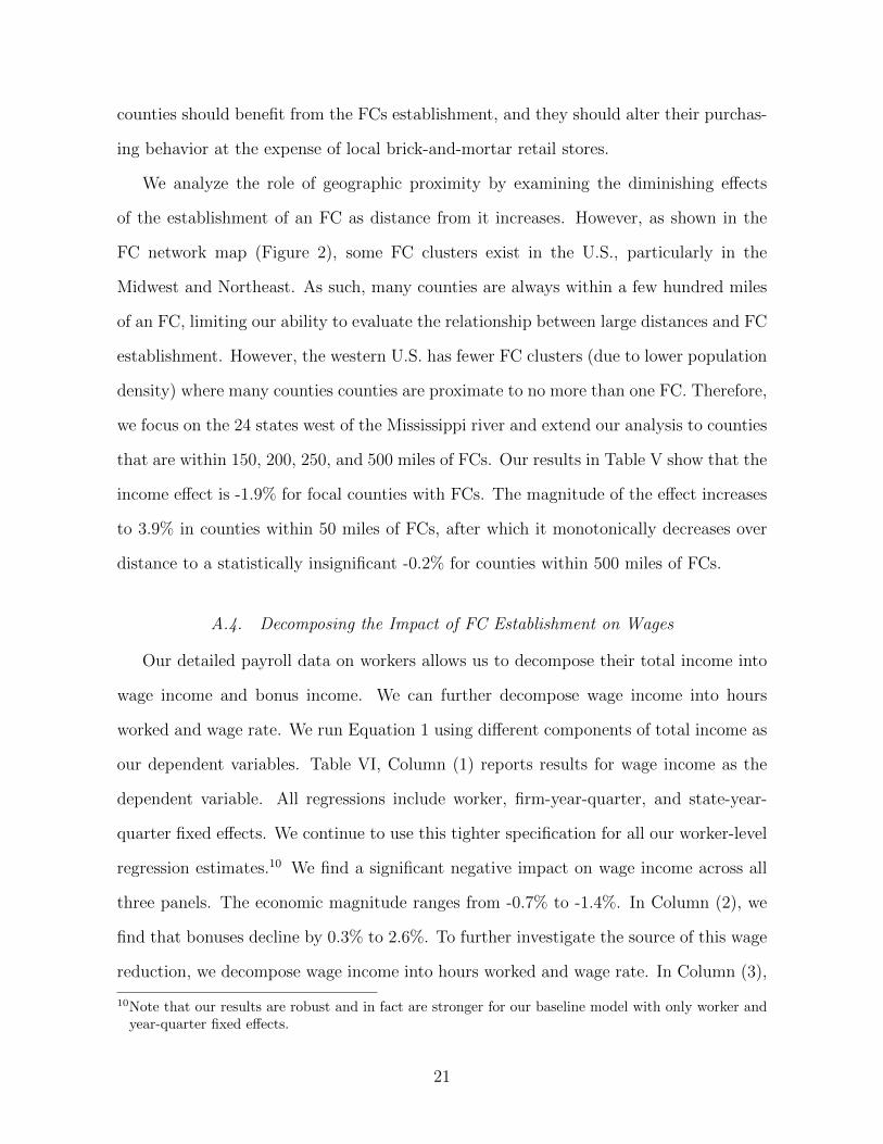
that are within 150, 200, 250, and 500 miles of FCs. Our results in Table V show that the

income effect is -1.9% for focal counties with FCs. The magnitude of the effect increases

to 3.9% in counties within 50 miles of FCs, after which it monotonically decreases over

distance to a statistically insignificant -0.2% for counties within 500 miles of FCs.

A.4. Decomposing the Impact of FC Establishment on Wages

Our detailed payroll data on workers allows us to decompose their total income into

wage income and bonus income. We can further decompose wage income into hours

worked and wage rate. We run Equation 1 using different components of total income as

our dependent variables. Table VI, Column (1) reports results for wage income as the

dependent variable. All regressions include worker, firm-year-quarter, and state-year-

quarter fixed effects. We continue to use this tighter specification for all our worker-level

regression estimates.10 We find a significant negative impact on wage income across all

three panels. The economic magnitude ranges from -0.7% to -1.4%. In Column (2), we

find that bonuses decline by 0.3% to 2.6%. To further investigate the source of this wage

reduction, we decompose wage income into hours worked and wage rate. In Column (3),

10Note that our results are robust and in fact are stronger for our baseline model with only worker andyear-quarter fixed effects.

21

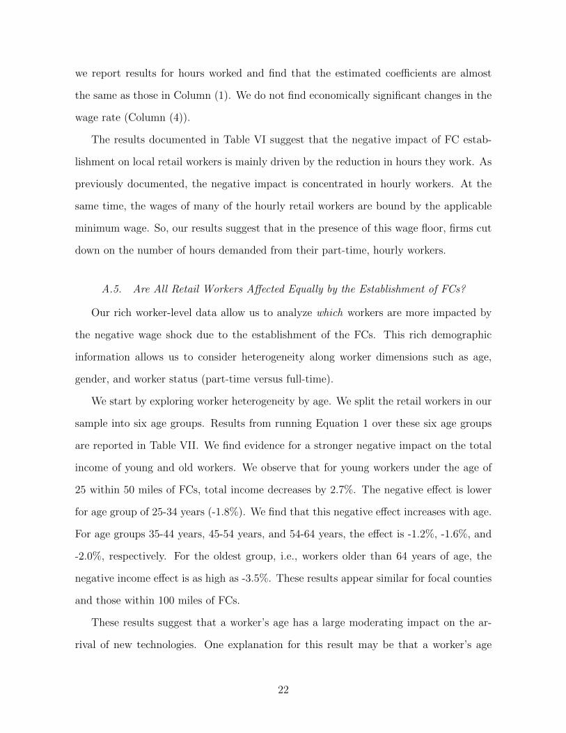
we report results for hours worked and find that the estimated coefficients are almost

the same as those in Column (1). We do not find economically significant changes in the

wage rate (Column (4)).

The results documented in Table VI suggest that the negative impact of FC estab-

lishment on local retail workers is mainly driven by the reduction in hours they work. As

previously documented, the negative impact is concentrated in hourly workers. At the

same time, the wages of many of the hourly retail workers are bound by the applicable

minimum wage. So, our results suggest that in the presence of this wage floor, firms cut

down on the number of hours demanded from their part-time, hourly workers.

A.5. Are All Retail Workers Affected Equally by the Establishment of FCs?

Our rich worker-level data allow us to analyze which workers are more impacted by

the negative wage shock due to the establishment of the FCs. This rich demographic

information allows us to consider heterogeneity along worker dimensions such as age,

gender, and worker status (part-time versus full-time).

We start by exploring worker heterogeneity by age. We split the retail workers in our

sample into six age groups. Results from running Equation 1 over these six age groups

are reported in Table VII. We find evidence for a stronger negative impact on the total

income of young and old workers. We observe that for young workers under the age of

25 within 50 miles of FCs, total income decreases by 2.7%. The negative effect is lower

for age group of 25-34 years (-1.8%). We find that this negative effect increases with age.

For age groups 35-44 years, 45-54 years, and 54-64 years, the effect is -1.2%, -1.6%, and

-2.0%, respectively. For the oldest group, i.e., workers older than 64 years of age, the

negative income effect is as high as -3.5%. These results appear similar for focal counties

and those within 100 miles of FCs.

These results suggest that a worker’s age has a large moderating impact on the ar-

rival of new technologies. One explanation for this result may be that a worker’s age

22

proxies for their productivity and accumulated firm-specific human capital. On the one

hand, young workers may be more productive, but firms may not have invested much

in enhancing their firm-specific human capital. On the other hand, old workers may

have accumulated firm-specific human capital but may be less productive compared to

younger workers. Explaining how age plays a prominent role is outside the scope of our

paper; however, our results at the least suggest that both younger and older workers

shoulder a disproportionate share of the negative impact of FC establishment as opposed

to middle-age workers.

Next, we test how the negative income effect varies across worker’s working status,

i.e., part-time workers versus full-time workers. Similar to age, a worker’s working status

may reflect his or her underlying level of firm-specific human capital accumulation. Firms

may invest more in the human capital development of full-time workers than part-time

workers. We define a worker as a part-time worker if the hours worked is less than 32

hours per week, otherwise the worker is considered a full-time worker. We define the

worker’s employment status in a time-invariant fashion by categorizing each worker by

their work status at the beginning of our sample period, i.e., in 2010Q1. Table VIII,

Panel A reports the differential effect on part-time and full-time workers. In line with

the hour reduction results previously reported, we find that the negative effect is stronger

for part-time workers, i.e., the impact on part-time workers is about -1% more.

It is possible that the negative impact of FCs varies by gender, given the significant

fraction of female retail employees. We test whether there is any differential effect of FCs

on male versus female workers. Table VIII, Panel B suggests that there is no difference

in the effect based on worker gender.

In summary, the heterogeneity in the negative impact of establishment of FCs may

be relevant for designing remedial responses to the negative impact of establishment

of FCs on local retail employees. We find that young and old workers (as opposed to

middle-aged workers) and part-time workers (as opposed to full-time workers) experience

23

disproportionately more negative effects from the establishment of FCs in their focal and

proximate counties.

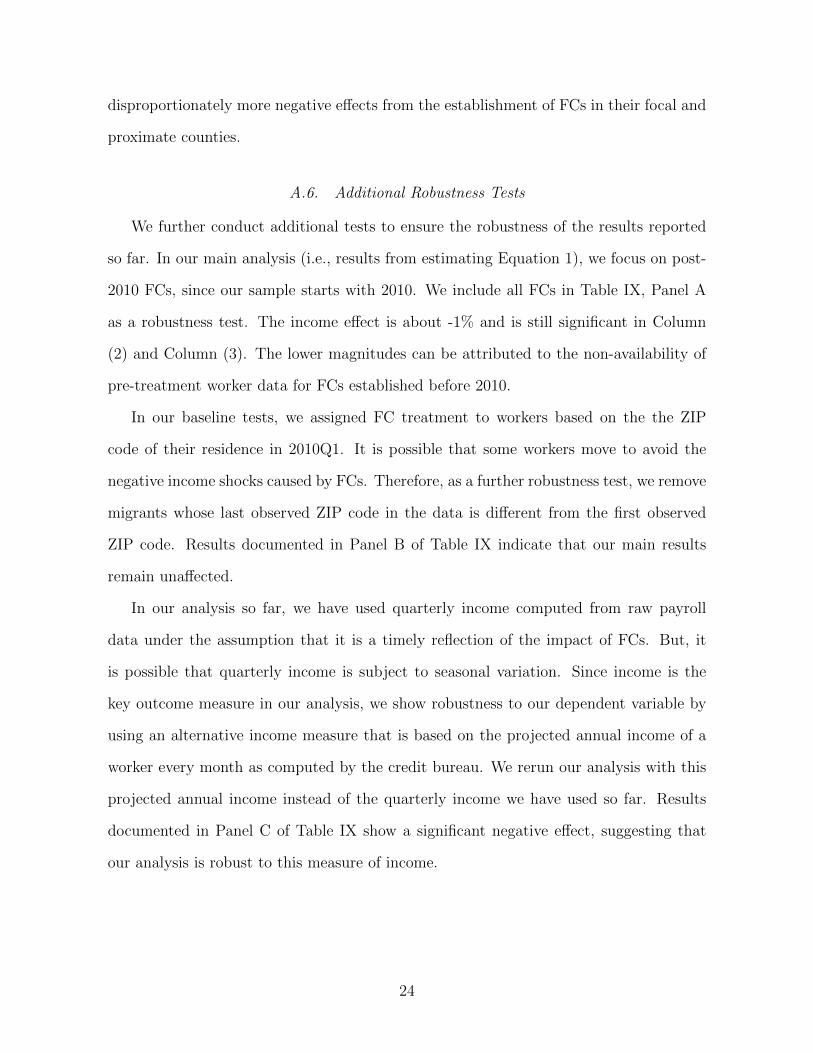
A.6. Additional Robustness Tests

We further conduct additional tests to ensure the robustness of the results reported

so far. In our main analysis (i.e., results from estimating Equation 1), we focus on post-

2010 FCs, since our sample starts with 2010. We include all FCs in Table IX, Panel A

as a robustness test. The income effect is about -1% and is still significant in Column

(2) and Column (3). The lower magnitudes can be attributed to the non-availability of

pre-treatment worker data for FCs established before 2010.

In our baseline tests, we assigned FC treatment to workers based on the the ZIP

code of their residence in 2010Q1. It is possible that some workers move to avoid the

negative income shocks caused by FCs. Therefore, as a further robustness test, we remove

migrants whose last observed ZIP code in the data is different from the first observed

ZIP code. Results documented in Panel B of Table IX indicate that our main results

remain unaffected.

In our analysis so far, we have used quarterly income computed from raw payroll

data under the assumption that it is a timely reflection of the impact of FCs. But, it

is possible that quarterly income is subject to seasonal variation. Since income is the

key outcome measure in our analysis, we show robustness to our dependent variable by

using an alternative income measure that is based on the projected annual income of a

worker every month as computed by the credit bureau. We rerun our analysis with this

projected annual income instead of the quarterly income we have used so far. Results

documented in Panel C of Table IX show a significant negative effect, suggesting that

our analysis is robust to this measure of income.

24

A.7. Credit Outcomes

Our results so far indicate that the establishment of FCs by a major online retailer has

a negative impact on the wages of workers at traditional brick-and-mortar retail stores in

the focal county and geographically proximate counties. The effects are predominantly

borne by young and old workers as opposed to middle-aged workers, part-time workers

as opposed to full-time workers, and hourly workers as opposed to salaried employees.

However, to the extent that labor markets are frictionless (i.e., workers can easily

switch jobs, and skills are completely transferable) the short-term displacement of some

traditional retail store workers that we document may not matter for the workers or

the local economy. However, in the presence of labor market frictions, the short-term

impact on the workers and local economy can be negative. Moreover, to the extent that

the scope of work differs between traditional retail stores and warehouses, at least some

workers can be worse off.

Our data prevent us from identifying any other source of income for the affected

workers, specifically part-time and hourly workers, except income from their primary

employer in the credit bureau payroll database. So, we are unable to directly verify

whether the affected workers offset the reduced hours with brick-and-mortar retail stores

by picking up additional working hours with another employer (who may not be part of

the payroll database that we use).

We test for this possibility indirectly by considering the credit outcomes of the work-

ers. If workers can easily substitute their sources of income, then it should have no effect

on their credit outcomes. Otherwise, the declines in income may lead to worse credit

outcomes, especially for the workers who are already living at the margin (i.e., workers

with high bank card utilization). We use credit score as a measure of the credit outcomes

for the affected workers. We assign a worker to the high utilization group if her bank

card utilization is higher than the median utilization ratio, and we assign workers to the

low utilization group if their bank card utilization is lower than the median.

25

We report our results in Table X. We find that the credit score for workers with high

utilization of bank credit cards declines significantly. In counties with FCs, the decreases

in credit scores of workers in the high utilization group are 3 points more than that of

workers in the low utilization group. It seems that the decline in credit scores is driven

by a higher bank credit card delinquency among the affected workers.

Overall, the evidence suggests that technological change, as manifested by an e-

commerce retailer establishing an FC, leads to a decline in wages for workers in tra-

ditional brick-and-mortar stores. Among the affected workers, those who have a prior

higher credit card utilization and those who are otherwise more financially vulnerable ex-

perience higher credit card delinquencies and a subsequent decline in their credit score.

These results suggest that some of the affected retail workers experience some frictions in

the labor market that preclude them from mitigating the extent to which the establish-

ment of e-commerce FCs in their county depresses their wage income and subsequently

their credit scores.

B. How Do FCs Affect Local Brick-and-Mortar Retail Stores? Evidence from NETS

Data

So far, we have used detailed worker level data and the staggered establishment of

FCs of the e-commerce retailer to understand the impact on the wages of the workers at

traditional brick-and-mortar retail stores in the focal county and geographically proxi-

mate counties. We next use NETS establishment-level data in order to understand the

impact of the establishment of FCs on traditional brick-and-mortar retail stores them-

selves. This analysis could highlight the aggregate implications of the negative income

effects that workers suffer when they work fewer hours.

B.1. Effect on Retail Store Sales

In Table XI, we use NETS data to understand the effect of FCs on the sales of

local brick-and-mortar stores. Column (1) reports difference-in-differences estimates for

26

all stores in the counties with FCs. In all the specifications, we include establishment

fixed effects, 6-digit NAICS-year fixed effects, and state-year fixed effects. We find that

the annual sales of local brick-and-mortar retail stores decrease by 2.8% (equivalent to

$63,639 per store) after the establishment of an FC of an e-commerce retailer.

In the next three columns, we partition the incumbent establishment/store sample

into terciles based on sales one year before the establishment of FCs in the county. We

find that for the bottom tercile (Small), the annual sales decrease by 2.9%, which is

equivalent to $7,565 per store. For the medium group (Medium), we find that sales

decrease by 2%, which is equivalent to $12,348 per store. For the top group (Large),

sales decrease by 3.4%, which is equivalent to $200,389 per store. These results suggest

that the establishment of FCs negatively affects the sales of local brick-and-mortar stores,

especially large retail stores. The effect is diminished in counties that are 50 or 100 miles

from FCs.

These results also suggest that after the staggered establishment of the e-commerce

firm’s FCs, sales decline significantly in the focal county of the FC. This decline in sales

may result in financial stress on the store, or it may motivate the parent company to

focus on improving the operational performance of the store. One consequence of the

decline in sales may be a reduction in the number of hours of work assigned to part-time

and hourly workers.

B.2. Effect on Retail Store Employment

So far, we find that the establishment of FCs negatively affects the income of retail

workers and the sales of local brick-and-mortar stores. Thus, it is instructive to un-

derstand how stores respond to lower sales after the increase in competition due to the

establishment of the e-commerce retailer’s FCs. Do they also adjust overall employment

levels in addition to reducing the number of hours of part-time and hourly workers?

Table XII reports results for the effect of FCs on local establishment-level employment.

27

The results appear similar to sales. Column (1) reports difference-in-differences estimates

for all stores in counties with FCs. We find that for all stores, employment decreases by

2.4%, which is equivalent to a reduction in employees of 41 workers per 100 stores for a

store with an average of 22 employees. For small stores, employment decreases by 2.7%,

which is equivalent to reducing 11 workers per 100 stores for a store with an average of 4

employees. For large stores, employment decreases by 1 worker per store for a store with

an average of 40 employees. Similar to sales results, the effect is diminished in counties

that are 50 or 100 miles of an FC.

Based on the results presented in the previous two subsections, it appears that after

the establishment of the e-commerce retailer’s FCs, traditional brick-and-mortar retail

stores in the focal county adjust to the decline in the sales both by reducing the number of

hours of work assigned to part-time and hourly workers and also by reducing employment

levels.

B.3. Closures of Retail Stores

Next, we analyze whether the increase in competition and the consequent decline in

store sales after the establishment of the e-commerce retailer’s FCs can lead, in extreme

cases, to an increase in retail store closures.

In Tables XIII and XIV, we attempt to understand whether the establishment of

FCs leads to store closures and how this effect varies with store size and age. Here we

define exit, our dependent variable, as a dummy equal to 1 if the establishment ceases

to exist one year before the end of the sample period, and 0 otherwise. Table XIII,

Panel A, Column (1) reports results for all stores.We find that the exit rate increases by

almost 3%. The average exit rate in our sample is almost 13.6%. The effect is negatively

correlated with the ex ante size of the store, i.e., small stores are more likely to exit than

large stores. This effect is consistent for counties 50 miles or 100 miles from a FC.

We further test the role of a store’s age on exits, and we report the results in Ta-

28

ble XIV. Here, we partition the All stores further into terciles, i.e., young, medium, and

old based on ex ante age. The average age in the bottom tercile is about eight years. We

find that young stores are more likely to close.

So, based on the analysis in Tables XIII and XIV, it appears that there is an increase

in the exit rate of local brick-and-mortar retail stores after the establishment of the FCs

of the e-commerce retailer. This exit rate impact is more pronounced for young and small

retail stores, as they are likely to be more financially stressed and may not be able to

survive the decline in sales after the FCs are established in the focal county.

B.4. Entry of Retail Stores

In all of our previous analysis, we focus on the effect of the establishment of FCs

on incumbent brick-and-mortar retail stores. But it is possible that entry into the local

retail sector is discouraged by the establishment of the FC, the consequent increase in

competition, and the decline in sales and closure of some of the incumbent brick-and-

mortar retail stores. We analyze the impact of the establishment of the FC on entry into

the local retail market in Table XV. Column (1) of Panel A reports county-level results

on the number of entrants. We find that after the establishment of an FC in the affected

county, the entry rate for small stores is significantly reduced by 11.8%. This low entry

rate effect is not just limited to counties with FCs; it also persists in counties 50 or 100

miles from an FC.

B.5. Effect on Sales of Full-Service Restaurants

We have attempted to rule out the key competing alternate explanation for the pattern

we observe in our data: the possibility that our results are driven by some omitted

local economic conditions and not by the establishment of the e-commerce retailer’s

FC in the county. As a further test to reduce the concerns about this interpretation,

we test whether FCs have any effect on the sales of local full-service restaurants. If

some omitted local economic shock is positively correlated with the establishment of an

29

FC in the affected counties, we would expect that the sales of full-service restaurants

(another important non-tradable sector) also respond to this negative economic shock

and experience a decrease in the focal counties.

Table XVI reports the results for the effect of FCs on the sales of full-service restau-

rants. Panel A, column (1) reports difference-in-differences estimates for all full-service

restaurants. We do not find any negative effect on sales of full-service restaurants with

the establishment of FCs in the counties. Similar to the previous subsection, we parti-

tion the data into terciles based on ex ante sales. We find that sales of small restaurants

increase in the focal counties, but we do not find any effect on sales for medium- or large-

sized restaurants nor any effect within 50 or 100 miles of FCs. These results indicate

that it is unlikely that an omitted local economic shock is responsible for the negative

impact on the sales of traditional brick-and-mortar retailers.

In summary, using detailed establishment level data from NETS, we find that after

the staggered establishment of the FCs of the e-commerce retailer, the geographically

proximate traditional brick-and-mortar retail stores experience a decline in sales, a decline

in employment, a decline in entry in the local retail sector, and an increase in closures

among the incumbent firms. The impact on store closures is more pronounced for young

stores and small stores, whereas the decline in sales is more pronounced for larger stores.

In addition, as a placebo, we find that the staggered establishment of the FCs of the

e-commerce retailer does not correlate with the sales of full-service restaurants. Overall,

our results suggest that the establishment of the e-commerce retailer’s FCs has a negative

impact on the financial health of the local traditional brick-and-mortar retail stores.

C. How Do FCs Affect Local Wages and Employment? Evidence from BLS County-

Industry Data

Finally, to understand the aggregate effect at the county level, we use county-level

QCEW data on total wages, employment level, average wage, and number of establish-

30

ments for each county. We report the results of the analysis in Table XVII. Using

county-level QCEW data, we find that the establishment of an FC has a negative effect

on local wages and employment. This is consistent with evidence using payroll data and

NETS establishment-level data. After absorbing 6-digit NAICS-year quarter fixed effects

and state-year quarter fixed effects, we find a muted effect for the counties with FCs, but

we find a very strong negative effect on total wages, employment level, average wage, and

number of establishments for counties within 50 or 100 miles of FCs. We further test for

pre-trends for all the counties within 50 miles (including the focal county), and we find

no pre-trends. Overall, the results using county-level QCEW data are largely supportive

of our findings using administrative employment data and NETS data.

V. Conclusion

The recent disruption in the retail sector can be attributed to the rise of e-commerce.

At the beginning of 2017, e-commerce sales accounted for 8.3% of total retail sales in the

U.S., compared to 3.8% in 2010. We use the staggered rollout of a major e-commerce

retailer’s FCs as a proxy for local e-commerce presence. Using a payroll dataset for 2.6

million retail workers, we find that the labor income of retail workers in counties with

FCs, on average, decreases by 2.4% after the establishment of FCs. Wages of hourly

workers decrease significantly by 2.5%, equivalent to $825. Most of the effect comes from

a reduction in the number of hours worked.

Further, using sales and employment data for 3.2 million stores, we find that retail

stores in counties with FCs experience a reduction in sales and employees. We find that

for stores in the top tercile based on sales one year before the FC, after the establish-

ment of FCs in their county, their sales decrease by almost 3.4%, which is equivalent to

$200,389 per store. For these stores, after the establishment of FCs in their county, their

employment decreases by almost 2.5%, which is equivalent to one worker per store for a

store with an average of 40 employees. Also, there is a decrease in entry and an increase

31

in exits for stores in the retail sector, with small and young retail stores exiting at a

higher rate. We find that the opening of FCs has no impact on the sales of a full-service

restaurant, which supports the proposition that negative local economic shocks may not

drive our results.

Overall, our results highlight how the dramatic increase in e-commerce retail sales

can have adverse consequences for workers at traditional brick-and-mortar stores. At the

same time, our results should be interpreted carefully in light of the many benefits of

e-commerce. In this paper, we do not consider the impact of e-commerce on consumers,

the increase in employment by the e-commerce firm, or the e-commerce firm’s ecosystem

and the ancilliary benefits to the county. Further, we do not consider the long-term

dynamics of the labor market in the counties affected by the FCs nor do we consider the

long-term effects on the traditional brick-and-mortar retail workers who are affected by

the establishment of e-commerce FCs in the focal county. Given the limited scope of this

paper, we do not aim to quantify the aggregate effect of e-commerce on the retail sector.

Our results can only show that the growth of e-commerce has some adverse consequences

for some traditional brick-and-mortar retail workers, and they can provide one piece of

evidence to help fully quantify the impact of e-commerce.

32

References

Acemoglu, Daron, 2002, Technical Change, Inequality, and the Labor Market, Jour-nal of Economic Literature 40, 7-72.

Autor, David H., 2015, Why Are There Still So Many Jobs? The History and Futureof Workplace Automation, Journal of Economic Perspectives 29, 3-30.

Autor, David H., David Dorn, and Gordon H. Hanson, 2013, The China Syndrome:Local Labor Market Effects of Import Competition in the United States, AmericanEconomic Review 103, 2121-2168.

Autor, David H., David Dorn, and Gordon H. Hanson, 2015, Untangling Tradeand Technology: Evidence from Local Labour Markets, The Economic Journal 125,621-646.

Autor, David H., David Dorn, Gordon H. Hanson, and Jae Song, 2014, Trade Ad-justment: Worker-Level Evidence, Quarterly Journal of Economics 129, 1799-1860.

Autor, David H., Lawrence F. Katz, and Alan B. Krueger, 1998, Computing Inequal-ity: Have Computers Changed the Labor Market? Quarterly Journal of Economics113, 1169-1213.

Autor, David H., Frank Levy, and Richard J. Murnane, 2003, The Skill Contentof Recent Technological Change: An Empirical Exploration, Quarterly Journal ofEconomics 118, 1279-1333.

Basker, Emek, 2005, Job Creation or Destruction? Labor Market Effects of Wal-Mart Expansion, Review of Economics and Statistics 87, 174-183.

Baugh, Brian, Itzhak Ben-David, and Hoonsuk Park, forthcoming, Can Taxes Shapeand Industry? Evidence from the Implementation of the ”Amazon Tax”, Journal ofFinance

Brynjolfsson, Erik, Yu Hu, and Michael D. Smith, 2003, Consumer Surplus in theDigital Economy: Estimating the Value of Increased Product Variety at OnlineBooksellers, Management Science 49, 1580-1596.

Brynjolfsson, Erik, and Andrew McAfee, 2011, Race Against the Machine, DigitalFrontier Press.

Brynjolfsson, Erik, and Andrew McAfee, 2014, The Second Machine Age: Work,Progress, and Prosperity in a Time of Brilliant Technologies, W.W. Norton & Com-pany.

Brynjolfsson, Erik, and Michael D. Smith, 2000, Frictionless Commerce? A Com-parison of Internet and Conventional Retailers, Management Science 46, 563-585.

33

Ghose, Anindya, Michael D. Smith, and Rahul Telang, 2006, Internet Exchangesfor Used Books: An Empirical Analysis of Product Cannibalization and WelfareImpact, Information Systems Research 17, 3-19.

Holmes, Thomas, 2011, The Diffusion of Wal-Mart and Economies of Density, Econo-metrica 79, 253-302.

Houde, Jean-Francois, Peter Newberry, and Katja Seim, 2017, Economies of Densityin E-Commerce: A Study of Amazon’s Fulfillment Center Network, Working Paper.

Jia, Panle, 2008, What Happens When Wal-Mart Comes to Town: An EmpiricalAnalysis of the Discount Retailing Industry, Econometrica 76, 1263-1316.

Krueger, Alan B., How Computers Have Changed the Wage Structure: Evidencefrom Microdata, 1984-1989, Quarterly Journal of Economics 108, 33-60.

National Academies of Sciences, Engineering, and Medicine, 2017, Information Tech-nology and the U.S. Workforce: Where Are We and Where Do We Go from Here?Washington, DC: The National Academies Press.

Neumark, David, Junfu Zhang, and Stephen Ciccarella, 2008, The Effects of Wal-Mart on Local Labor Markets, Journal of Urban Economics 63, 405-430.

Pozzi, Andrea, 2013, The Effect of Internet Distribution on Brick-and-Mortar Sales,RAND Journal of Economics 44, 569-583.

Stone, Brad, 2013, The Everything Store: Jeff Bezos and the Age of Amazon, Little,Brown and Company.

Subramani, Mani, and Eric Walden, 2001, The Impact of E-Commerce Announce-ments on the Market Value of Firms, Information System Research 12, 135-154.

Walls & Associates, 2014, The National Establishment Time-Series (NETS)Database, Denver, Colorado.

34

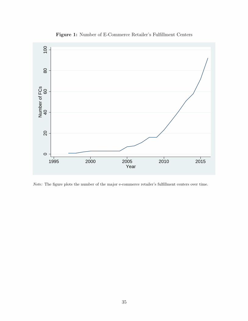
Figure 1: Number of E-Commerce Retailer’s Fulfillment Centers

020

4060

8010

0N

umbe

r of

FC

s

1995 2000 2005 2010 2015Year

Note: The figure plots the number of the major e-commerce retailer’s fulfillment centers over time.

35

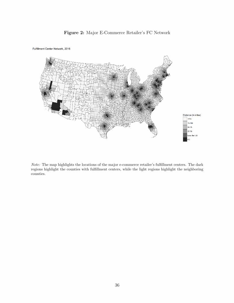
Figure 2: Major E-Commerce Retailer’s FC Network

Note: The map highlights the locations of the major e-commerce retailer’s fulfillment centers. The darkregions highlight the counties with fulfillment centers, while the light regions highlight the neighboringcounties.

36

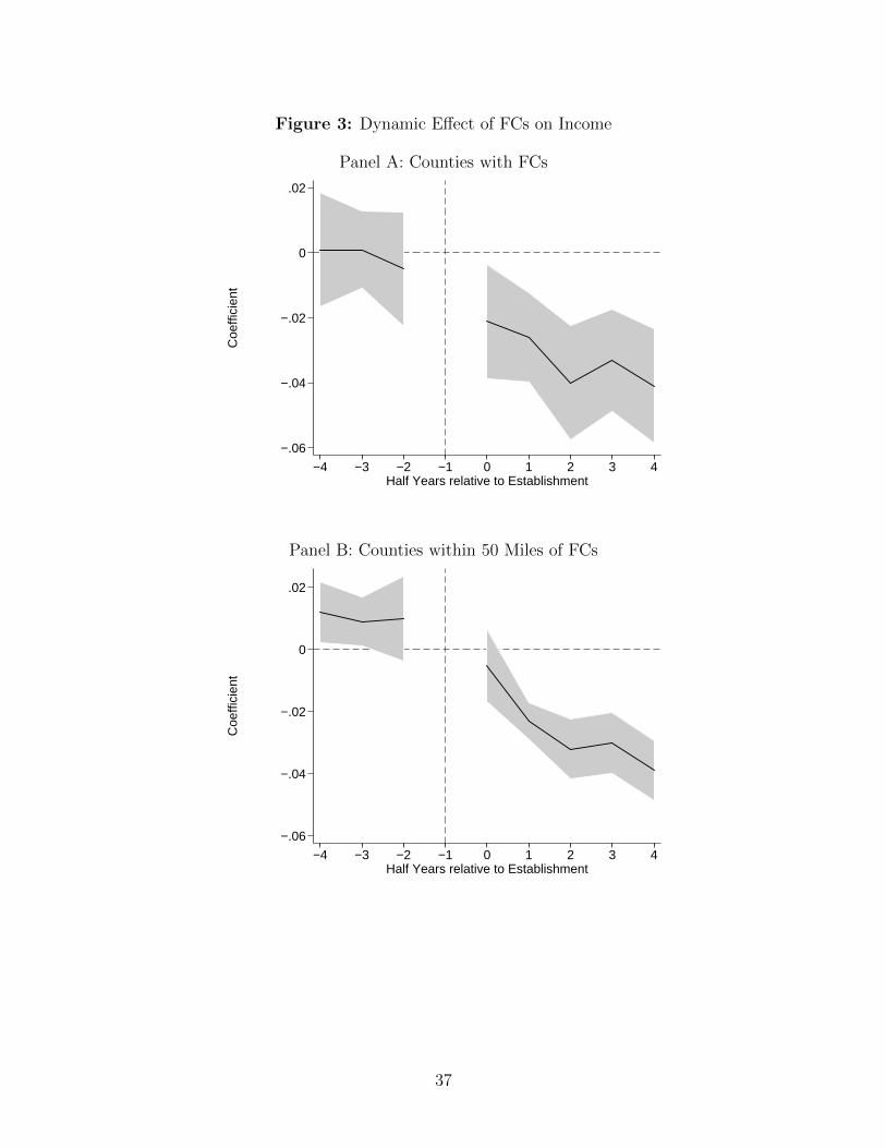
Figure 3: Dynamic Effect of FCs on Income

Panel A: Counties with FCs

−.06

−.04

−.02

0

.02

Coe

ffici

ent

−4 −3 −2 −1 0 1 2 3 4Half Years relative to Establishment

Panel B: Counties within 50 Miles of FCs

−.06

−.04

−.02

0

.02

Coe

ffici

ent

−4 −3 −2 −1 0 1 2 3 4Half Years relative to Establishment

37

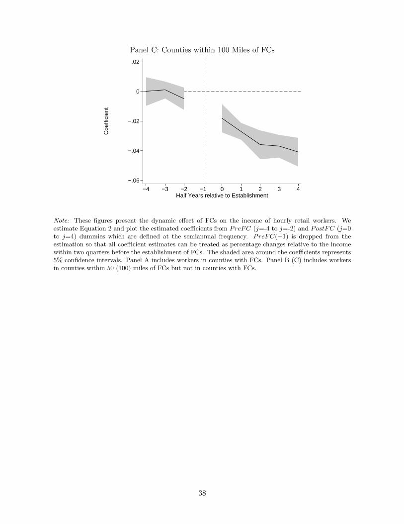
Panel C: Counties within 100 Miles of FCs

−.06

−.04

−.02

0

.02

Coe

ffici

ent

−4 −3 −2 −1 0 1 2 3 4Half Years relative to Establishment

Note: These figures present the dynamic effect of FCs on the income of hourly retail workers. Weestimate Equation 2 and plot the estimated coefficients from PreFC (j=-4 to j=-2) and PostFC (j=0to j=4) dummies which are defined at the semiannual frequency. PreFC(−1) is dropped from theestimation so that all coefficient estimates can be treated as percentage changes relative to the incomewithin two quarters before the establishment of FCs. The shaded area around the coefficients represents5% confidence intervals. Panel A includes workers in counties with FCs. Panel B (C) includes workersin counties within 50 (100) miles of FCs but not in counties with FCs.

38

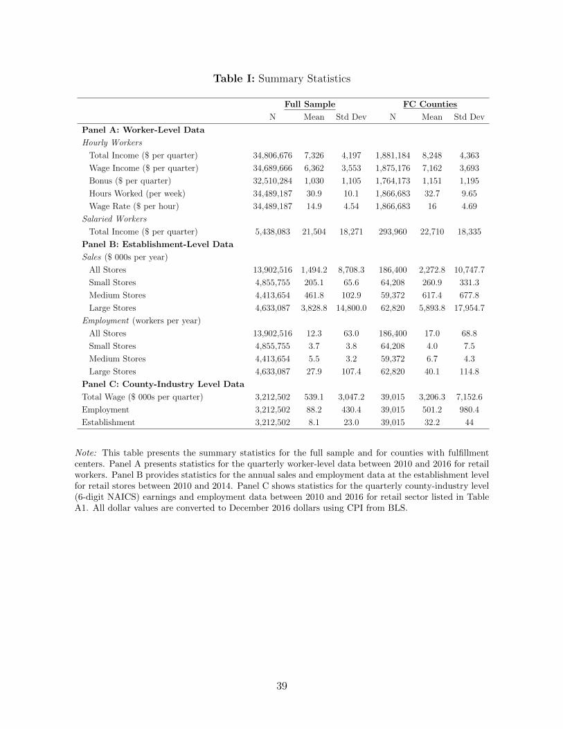
Table I: Summary Statistics

Full Sample FC Counties

N Mean Std Dev N Mean Std Dev

Panel A: Worker-Level Data

Hourly Workers

Total Income ($ per quarter) 34,806,676 7,326 4,197 1,881,184 8,248 4,363

Wage Income ($ per quarter) 34,689,666 6,362 3,553 1,875,176 7,162 3,693

Bonus ($ per quarter) 32,510,284 1,030 1,105 1,764,173 1,151 1,195

Hours Worked (per week) 34,489,187 30.9 10.1 1,866,683 32.7 9.65

Wage Rate ($ per hour) 34,489,187 14.9 4.54 1,866,683 16 4.69

Salaried Workers

Total Income ($ per quarter) 5,438,083 21,504 18,271 293,960 22,710 18,335

Panel B: Establishment-Level Data

Sales ($ 000s per year)

All Stores 13,902,516 1,494.2 8,708.3 186,400 2,272.8 10,747.7

Small Stores 4,855,755 205.1 65.6 64,208 260.9 331.3

Medium Stores 4,413,654 461.8 102.9 59,372 617.4 677.8

Large Stores 4,633,087 3,828.8 14,800.0 62,820 5,893.8 17,954.7

Employment (workers per year)

All Stores 13,902,516 12.3 63.0 186,400 17.0 68.8

Small Stores 4,855,755 3.7 3.8 64,208 4.0 7.5

Medium Stores 4,413,654 5.5 3.2 59,372 6.7 4.3

Large Stores 4,633,087 27.9 107.4 62,820 40.1 114.8

Panel C: County-Industry Level Data

Total Wage ($ 000s per quarter) 3,212,502 539.1 3,047.2 39,015 3,206.3 7,152.6

Employment 3,212,502 88.2 430.4 39,015 501.2 980.4

Establishment 3,212,502 8.1 23.0 39,015 32.2 44

Note: This table presents the summary statistics for the full sample and for counties with fulfillmentcenters. Panel A presents statistics for the quarterly worker-level data between 2010 and 2016 for retailworkers. Panel B provides statistics for the annual sales and employment data at the establishment levelfor retail stores between 2010 and 2014. Panel C shows statistics for the quarterly county-industry level(6-digit NAICS) earnings and employment data between 2010 and 2016 for retail sector listed in TableA1. All dollar values are converted to December 2016 dollars using CPI from BLS.

39

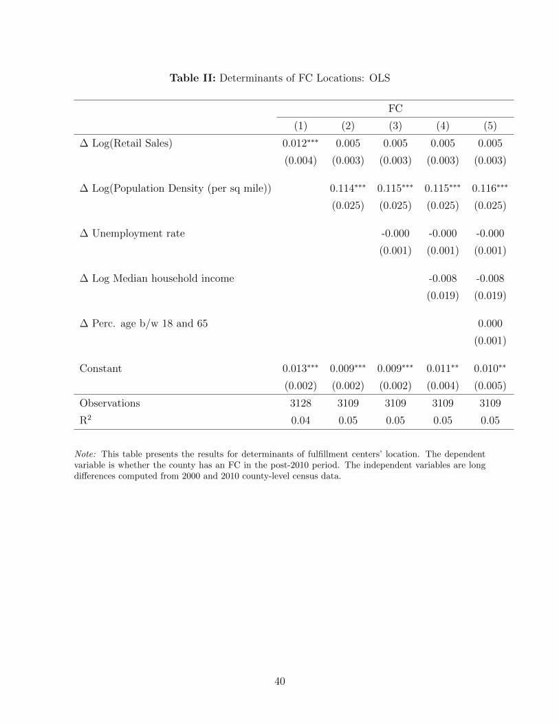
Table II: Determinants of FC Locations: OLS

FC

(1) (2) (3) (4) (5)

∆ Log(Retail Sales) 0.012∗∗∗ 0.005 0.005 0.005 0.005

(0.004) (0.003) (0.003) (0.003) (0.003)

∆ Log(Population Density (per sq mile)) 0.114∗∗∗ 0.115∗∗∗ 0.115∗∗∗ 0.116∗∗∗

(0.025) (0.025) (0.025) (0.025)

∆ Unemployment rate -0.000 -0.000 -0.000

(0.001) (0.001) (0.001)

∆ Log Median household income -0.008 -0.008

(0.019) (0.019)

∆ Perc. age b/w 18 and 65 0.000

(0.001)

Constant 0.013∗∗∗ 0.009∗∗∗ 0.009∗∗∗ 0.011∗∗ 0.010∗∗

(0.002) (0.002) (0.002) (0.004) (0.005)

Observations 3128 3109 3109 3109 3109

R2 0.04 0.05 0.05 0.05 0.05

Note: This table presents the results for determinants of fulfillment centers’ location. The dependentvariable is whether the county has an FC in the post-2010 period. The independent variables are longdifferences computed from 2000 and 2010 county-level census data.

40

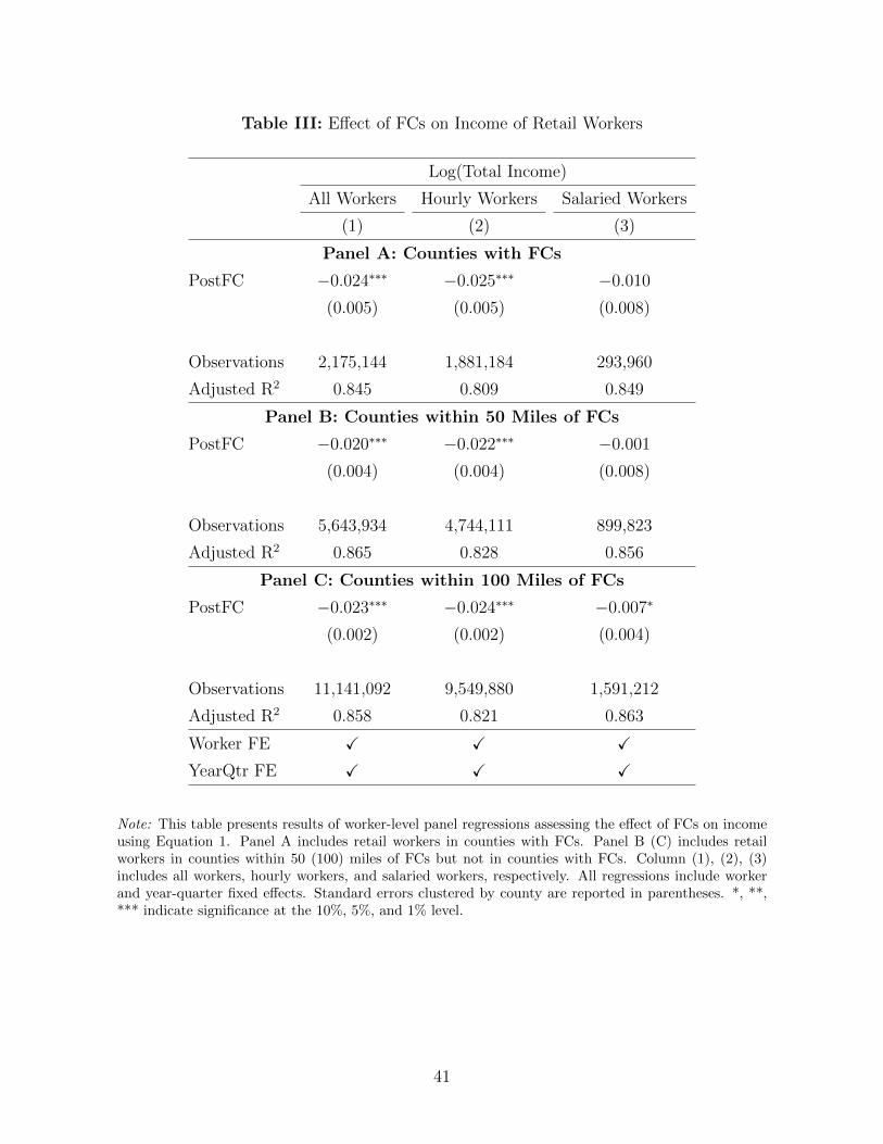
Table III: Effect of FCs on Income of Retail Workers

Log(Total Income)

All Workers Hourly Workers Salaried Workers

(1) (2) (3)

Panel A: Counties with FCs

PostFC −0.024∗∗∗ −0.025∗∗∗ −0.010

(0.005) (0.005) (0.008)

Observations 2,175,144 1,881,184 293,960

Adjusted R2 0.845 0.809 0.849

Panel B: Counties within 50 Miles of FCs

PostFC −0.020∗∗∗ −0.022∗∗∗ −0.001

(0.004) (0.004) (0.008)

Observations 5,643,934 4,744,111 899,823

Adjusted R2 0.865 0.828 0.856

Panel C: Counties within 100 Miles of FCs

PostFC −0.023∗∗∗ −0.024∗∗∗ −0.007∗

(0.002) (0.002) (0.004)

Observations 11,141,092 9,549,880 1,591,212

Adjusted R2 0.858 0.821 0.863

Worker FE X X X

YearQtr FE X X X

Note: This table presents results of worker-level panel regressions assessing the effect of FCs on incomeusing Equation 1. Panel A includes retail workers in counties with FCs. Panel B (C) includes retailworkers in counties within 50 (100) miles of FCs but not in counties with FCs. Column (1), (2), (3)includes all workers, hourly workers, and salaried workers, respectively. All regressions include workerand year-quarter fixed effects. Standard errors clustered by county are reported in parentheses. *, **,*** indicate significance at the 10%, 5%, and 1% level.

41

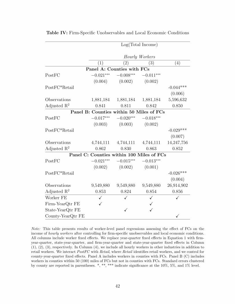
Table IV: Firm-Specific Unobservables and Local Economic Conditions

Log(Total Income)

Hourly Workers

(1) (2) (3) (4)

Panel A: Counties with FCs

PostFC −0.021∗∗∗ −0.008∗∗∗ −0.011∗∗∗

(0.004) (0.002) (0.002)

PostFC*Retail -0.044***

(0.006)

Observations 1,881,184 1,881,184 1,881,184 5,596,632

Adjusted R2 0.841 0.811 0.842 0.850

Panel B: Counties within 50 Miles of FCs

PostFC −0.017∗∗∗ −0.020∗∗∗ −0.018∗∗∗

(0.003) (0.003) (0.002)

PostFC*Retail -0.029***

(0.007)

Observations 4,744,111 4,744,111 4,744,111 14,247,756

Adjusted R2 0.862 0.830 0.863 0.852

Panel C: Counties within 100 Miles of FCs

PostFC −0.021∗∗∗ −0.015∗∗∗ −0.013∗∗∗

(0.002) (0.002) (0.001)

PostFC*Retail -0.026***

(0.004)

Observations 9,549,880 9,549,880 9,549,880 26,914,902

Adjusted R2 0.853 0.824 0.854 0.856

Worker FE X X X XFirm-YearQtr FE X XState-YearQtr FE X XCounty-YearQtr FE X

Note: This table presents results of worker-level panel regressions assessing the effect of FCs on theincome of hourly workers after controlling for firm-specific unobservables and local economic conditions.All columns include worker fixed effects. We replace year-quarter fixed effects in Equation 1 with firm-year-quarter, state-year-quarter, and firm-year-quarter and state-year-quarter fixed effects in Column(1), (2), (3), respectively. In Column (4), we include all hourly workers in other industries in addition toretail workers. We interact PostFC with Retail, where Retail identifies retail workers, and we control forcounty-year-quarter fixed effects. Panel A includes workers in counties with FCs. Panel B (C) includesworkers in counties within 50 (100) miles of FCs but not in counties with FCs. Standard errors clusteredby county are reported in parentheses. *, **, *** indicate significance at the 10%, 5%, and 1% level.

42

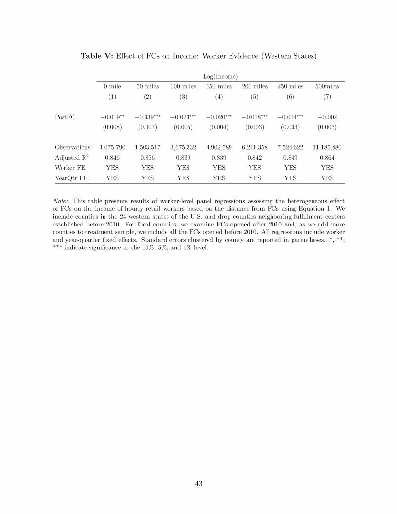
Table V: Effect of FCs on Income: Worker Evidence (Western States)

Log(Income)

0 mile 50 miles 100 miles 150 miles 200 miles 250 miles 500miles

(1) (2) (3) (4) (5) (6) (7)

PostFC −0.019∗∗ −0.039∗∗∗ −0.023∗∗∗ −0.020∗∗∗ −0.018∗∗∗ −0.014∗∗∗ −0.002

(0.008) (0.007) (0.005) (0.004) (0.003) (0.003) (0.003)

Observations 1,075,790 1,503,517 3,675,332 4,902,589 6,241,358 7,524,622 11,185,880

Adjusted R2 0.846 0.856 0.839 0.839 0.842 0.849 0.864

Worker FE YES YES YES YES YES YES YES

YearQtr FE YES YES YES YES YES YES YES

Note: This table presents results of worker-level panel regressions assessing the heterogeneous effectof FCs on the income of hourly retail workers based on the distance from FCs using Equation 1. Weinclude counties in the 24 western states of the U.S. and drop counties neighboring fulfillment centersestablished before 2010. For focal counties, we examine FCs opened after 2010 and, as we add morecounties to treatment sample, we include all the FCs opened before 2010. All regressions include workerand year-quarter fixed effects. Standard errors clustered by county are reported in parentheses. *, **,*** indicate significance at the 10%, 5%, and 1% level.

43

Table VI: Decomposition of Income Effect for Hourly Workers

Log(Wage Income) Log(Bonus) Log(Hours Worked) Log(Wage Rate)

(1) (2) (3) (4)

Panel A: Counties with FCs

PostFC -0.007*** -0.012 -0.007*** 0.001***

(0.002) (0.008) (0.002) (0.000)

Observations 1,875,176 1,764,173 1,866,683 1,866,683

Adjusted R2 0.842 0.740 0.731 0.970

Panel B: Counties within 50 Miles of FCs

PostFC -0.014*** -0.026*** -0.014*** -0.000

(0.002) (0.009) (0.002) (0.001)

Observations 4,730,532 4,414,584 4,711,647 4,711,647

Adjusted R2 0.856 0.744 0.761 0.968

Panel C: Counties within 100 Miles of FCs

PostFC -0.012*** -0.003 -0.011*** -0.001*

(0.001) (0.008) (0.001) (0.000)

Observations 9,521,947 8,921,138 9,476,710 9,476,710

Adjusted R2 0.849 0.746 0.744 0.969

Worker FE X X X X

Firm-YearQtr FE X X X X

State-YearQtr FE X X X X

Note: This table presents results of worker-level panel regressions assessing the effect of FCs on the wageincome, bonus, hours worked, and wage rate of hourly retail workers using Equation 1. Panel A includesworkers in counties with FCs. Panel B (C) includes workers in counties within 50 (100) miles of FCs butnot in counties with FCs. All regressions include worker, firm-year-quarter, and state-year-quarter fixedeffects. Standard errors clustered by county are reported in parentheses. *, **, *** indicate significanceat the 10%, 5%, and 1% level.

44

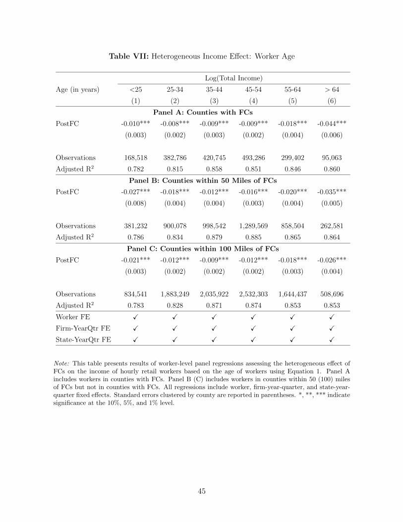
Table VII: Heterogeneous Income Effect: Worker Age

Log(Total Income)

Age (in years) <25 25-34 35-44 45-54 55-64 > 64

(1) (2) (3) (4) (5) (6)

Panel A: Counties with FCs

PostFC -0.010*** -0.008*** -0.009*** -0.009*** -0.018*** -0.044***

(0.003) (0.002) (0.003) (0.002) (0.004) (0.006)

Observations 168,518 382,786 420,745 493,286 299,402 95,063

Adjusted R2 0.782 0.815 0.858 0.851 0.846 0.860

Panel B: Counties within 50 Miles of FCs

PostFC -0.027*** -0.018*** -0.012*** -0.016*** -0.020*** -0.035***

(0.008) (0.004) (0.004) (0.003) (0.004) (0.005)

Observations 381,232 900,078 998,542 1,289,569 858,504 262,581

Adjusted R2 0.786 0.834 0.879 0.885 0.865 0.864

Panel C: Counties within 100 Miles of FCs

PostFC -0.021*** -0.012*** -0.009*** -0.012*** -0.018*** -0.026***

(0.003) (0.002) (0.002) (0.002) (0.003) (0.004)

Observations 834,541 1,883,249 2,035,922 2,532,303 1,644,437 508,696

Adjusted R2 0.783 0.828 0.871 0.874 0.853 0.853

Worker FE X X X X X X

Firm-YearQtr FE X X X X X X

State-YearQtr FE X X X X X X

Note: This table presents results of worker-level panel regressions assessing the heterogeneous effect ofFCs on the income of hourly retail workers based on the age of workers using Equation 1. Panel Aincludes workers in counties with FCs. Panel B (C) includes workers in counties within 50 (100) milesof FCs but not in counties with FCs. All regressions include worker, firm-year-quarter, and state-year-quarter fixed effects. Standard errors clustered by county are reported in parentheses. *, **, *** indicatesignificance at the 10%, 5%, and 1% level.

45

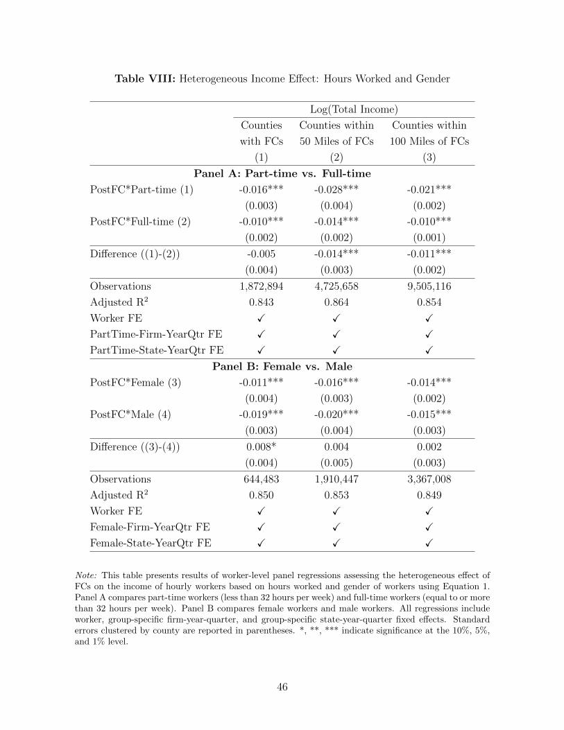
Table VIII: Heterogeneous Income Effect: Hours Worked and Gender

Log(Total Income)

Counties Counties within Counties within

with FCs 50 Miles of FCs 100 Miles of FCs

(1) (2) (3)

Panel A: Part-time vs. Full-time

PostFC*Part-time (1) -0.016*** -0.028*** -0.021***

(0.003) (0.004) (0.002)

PostFC*Full-time (2) -0.010*** -0.014*** -0.010***

(0.002) (0.002) (0.001)

Difference ((1)-(2)) -0.005 -0.014*** -0.011***

(0.004) (0.003) (0.002)

Observations 1,872,894 4,725,658 9,505,116

Adjusted R2 0.843 0.864 0.854

Worker FE X X X

PartTime-Firm-YearQtr FE X X X

PartTime-State-YearQtr FE X X X

Panel B: Female vs. Male

PostFC*Female (3) -0.011*** -0.016*** -0.014***

(0.004) (0.003) (0.002)

PostFC*Male (4) -0.019*** -0.020*** -0.015***

(0.003) (0.004) (0.003)

Difference ((3)-(4)) 0.008* 0.004 0.002

(0.004) (0.005) (0.003)

Observations 644,483 1,910,447 3,367,008

Adjusted R2 0.850 0.853 0.849

Worker FE X X X

Female-Firm-YearQtr FE X X X

Female-State-YearQtr FE X X X

Note: This table presents results of worker-level panel regressions assessing the heterogeneous effect ofFCs on the income of hourly workers based on hours worked and gender of workers using Equation 1.Panel A compares part-time workers (less than 32 hours per week) and full-time workers (equal to or morethan 32 hours per week). Panel B compares female workers and male workers. All regressions includeworker, group-specific firm-year-quarter, and group-specific state-year-quarter fixed effects. Standarderrors clustered by county are reported in parentheses. *, **, *** indicate significance at the 10%, 5%,and 1% level.

46

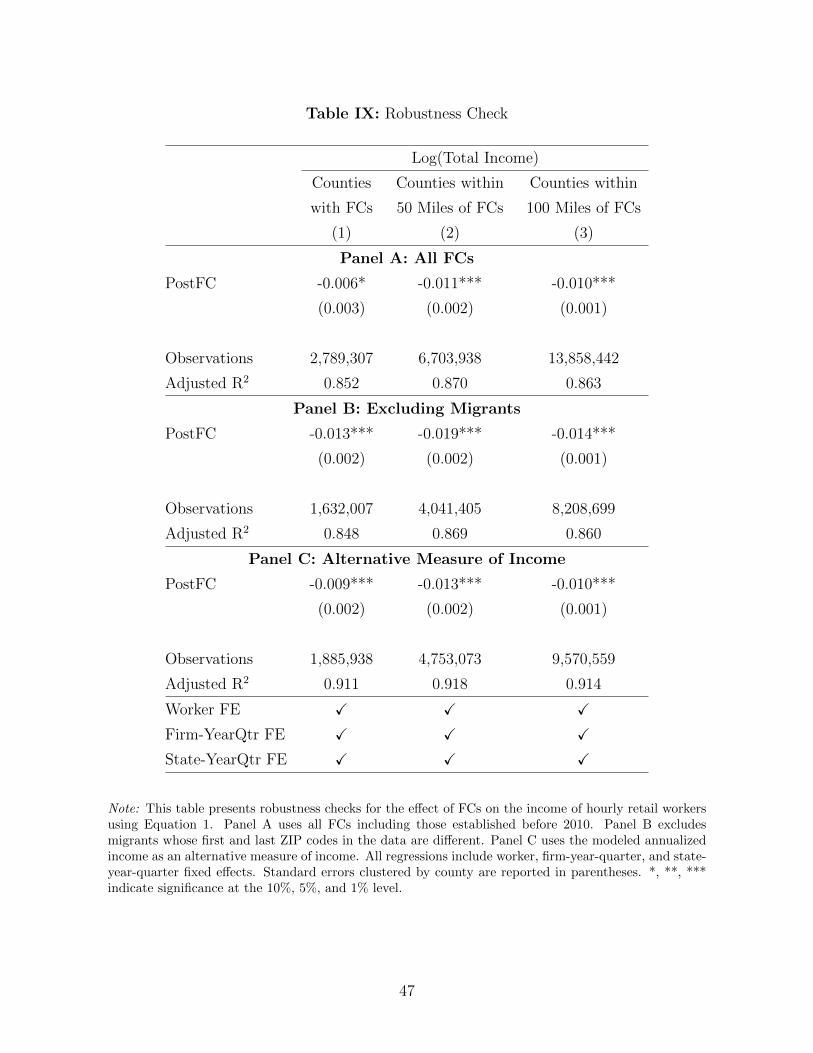
Table IX: Robustness Check

Log(Total Income)

Counties Counties within Counties within

with FCs 50 Miles of FCs 100 Miles of FCs

(1) (2) (3)

Panel A: All FCs

PostFC -0.006* -0.011*** -0.010***

(0.003) (0.002) (0.001)

Observations 2,789,307 6,703,938 13,858,442

Adjusted R2 0.852 0.870 0.863

Panel B: Excluding Migrants

PostFC -0.013*** -0.019*** -0.014***

(0.002) (0.002) (0.001)

Observations 1,632,007 4,041,405 8,208,699

Adjusted R2 0.848 0.869 0.860

Panel C: Alternative Measure of Income

PostFC -0.009*** -0.013*** -0.010***

(0.002) (0.002) (0.001)

Observations 1,885,938 4,753,073 9,570,559

Adjusted R2 0.911 0.918 0.914

Worker FE X X X

Firm-YearQtr FE X X X

State-YearQtr FE X X X

Note: This table presents robustness checks for the effect of FCs on the income of hourly retail workersusing Equation 1. Panel A uses all FCs including those established before 2010. Panel B excludesmigrants whose first and last ZIP codes in the data are different. Panel C uses the modeled annualizedincome as an alternative measure of income. All regressions include worker, firm-year-quarter, and state-year-quarter fixed effects. Standard errors clustered by county are reported in parentheses. *, **, ***indicate significance at the 10%, 5%, and 1% level.

47

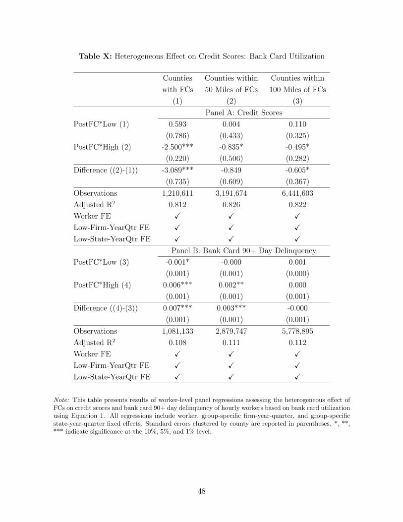
Table X: Heterogeneous Effect on Credit Scores: Bank Card Utilization

Counties Counties within Counties within

with FCs 50 Miles of FCs 100 Miles of FCs

(1) (2) (3)

Panel A: Credit Scores

PostFC*Low (1) 0.593 0.004 0.110

(0.786) (0.433) (0.325)

PostFC*High (2) -2.500*** -0.835* -0.495*

(0.220) (0.506) (0.282)

Difference ((2)-(1)) -3.089*** -0.849 -0.605*

(0.735) (0.609) (0.367)

Observations 1,210,611 3,191,674 6,441,603

Adjusted R2 0.812 0.826 0.822

Worker FE X X X

Low-Firm-YearQtr FE X X X

Low-State-YearQtr FE X X X

Panel B: Bank Card 90+ Day Delinquency

PostFC*Low (3) -0.001* -0.000 0.001

(0.001) (0.001) (0.000)

PostFC*High (4) 0.006*** 0.002** 0.000

(0.001) (0.001) (0.001)

Difference ((4)-(3)) 0.007*** 0.003*** -0.000

(0.001) (0.001) (0.001)

Observations 1,081,133 2,879,747 5,778,895

Adjusted R2 0.108 0.111 0.112

Worker FE X X X

Low-Firm-YearQtr FE X X X

Low-State-YearQtr FE X X X

Note: This table presents results of worker-level panel regressions assessing the heterogeneous effect ofFCs on credit scores and bank card 90+ day delinquency of hourly workers based on bank card utilizationusing Equation 1. All regressions include worker, group-specific firm-year-quarter, and group-specificstate-year-quarter fixed effects. Standard errors clustered by county are reported in parentheses. *, **,*** indicate significance at the 10%, 5%, and 1% level.

48

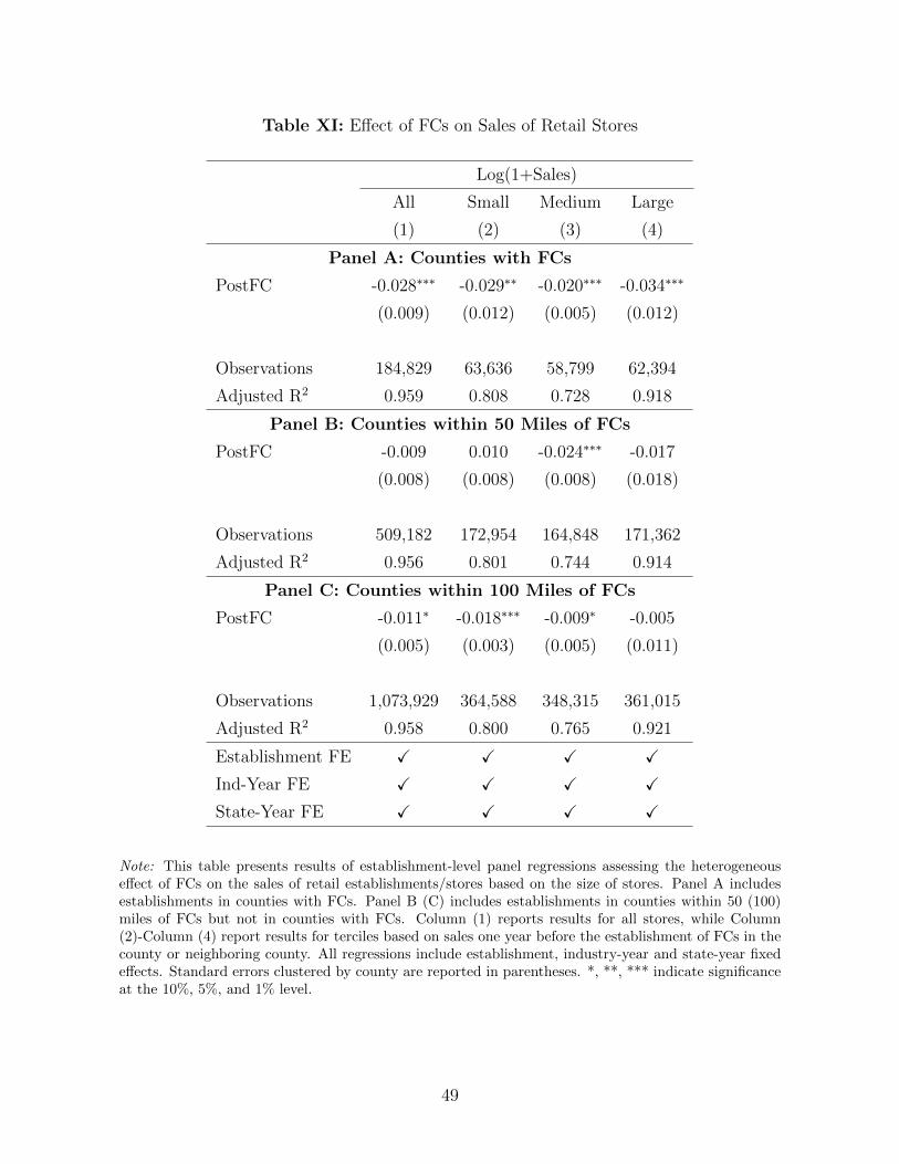
Table XI: Effect of FCs on Sales of Retail Stores

Log(1+Sales)

All Small Medium Large

(1) (2) (3) (4)

Panel A: Counties with FCs

PostFC -0.028∗∗∗ -0.029∗∗ -0.020∗∗∗ -0.034∗∗∗

(0.009) (0.012) (0.005) (0.012)

Observations 184,829 63,636 58,799 62,394

Adjusted R2 0.959 0.808 0.728 0.918

Panel B: Counties within 50 Miles of FCs

PostFC -0.009 0.010 -0.024∗∗∗ -0.017

(0.008) (0.008) (0.008) (0.018)

Observations 509,182 172,954 164,848 171,362

Adjusted R2 0.956 0.801 0.744 0.914

Panel C: Counties within 100 Miles of FCs

PostFC -0.011∗ -0.018∗∗∗ -0.009∗ -0.005

(0.005) (0.003) (0.005) (0.011)

Observations 1,073,929 364,588 348,315 361,015

Adjusted R2 0.958 0.800 0.765 0.921

Establishment FE X X X X

Ind-Year FE X X X X

State-Year FE X X X X

Note: This table presents results of establishment-level panel regressions assessing the heterogeneouseffect of FCs on the sales of retail establishments/stores based on the size of stores. Panel A includesestablishments in counties with FCs. Panel B (C) includes establishments in counties within 50 (100)miles of FCs but not in counties with FCs. Column (1) reports results for all stores, while Column(2)-Column (4) report results for terciles based on sales one year before the establishment of FCs in thecounty or neighboring county. All regressions include establishment, industry-year and state-year fixedeffects. Standard errors clustered by county are reported in parentheses. *, **, *** indicate significanceat the 10%, 5%, and 1% level.

49

Table XII: Effect of FCs on Employment of Retail Stores

Log(1+Employment)

All Small Medium Large

(1) (2) (3) (4)

Panel A: Counties with FCs

PostFC -0.024∗∗∗ -0.027∗∗∗ -0.019∗∗∗ -0.025∗∗∗

(0.007) (0.006) (0.005) (0.009)

Observations 184,829 63,636 58,799 62,394

Adjusted R2 0.973 0.871 0.907 0.955

Panel B: Counties within 50 Miles of FCs

PostFC -0.007 -0.003 -0.015∗∗∗ -0.005

(0.004) (0.003) (0.005) (0.007)

Observations 509,182 172,954 164,848 171,362

Adjusted R2 0.973 0.875 0.912 0.956

Panel C: Counties within 100 Miles of FCs

PostFC -0.008∗∗ -0.011∗∗∗ -0.007∗∗ -0.005

(0.003) (0.003) (0.003) (0.004)

Observations 1,073,929 364,588 348,315 361,015

Adjusted R2 0.978 0.883 0.924 0.969

Establishment FE X X X X

Ind-Year FE X X X X

State-Year FE X X X X

Note: This table presents results of establishment-level panel regressions assessing the heterogeneouseffect of FCs on the employment of retail establishments/stores based on the size of stores. Panel Aincludes establishments in counties with FCs. Panel B (C) includes establishments in counties within 50(100) miles of FCs but not in counties with FCs. Column (1) reports results for all stores, while Column(2)-Column (4) report results for terciles based on sales one year before the establishment of FCs in thecounty or neighboring county. All regressions include establishment, industry-year and state-year fixedeffects. Standard errors clustered by county are reported in parentheses. *, **, *** indicate significanceat the 10%, 5%, and 1% level.

50

Table XIII: Retail Store Closures: Size Effect

Exit

All Small Medium Large

(1) (2) (3) (4)

Panel A: Counties with FCs

PostFC 0.029∗∗∗ 0.038∗∗ 0.027∗∗∗ 0.023∗∗∗

(0.010) (0.014) (0.009) (0.007)

Observations 161,520 53,753 53,470 54,297

Adjusted R2 0.214 0.222 0.213 0.207

Panel B: Counties within 50 Miles of FCs

PostFC 0.023∗∗∗ 0.035∗∗∗ 0.022∗∗∗ 0.012∗∗

(0.007) (0.009) (0.007) (0.005)

Observations 446,770 148,440 148,708 149,604

Adjusted R2 0.202 0.207 0.201 0.200

Panel C: Counties within 100 Miles of FCs

PostFC 0.014∗∗∗ 0.020∗∗∗ 0.012∗∗ 0.011∗∗∗

(0.004) (0.005) (0.005) (0.003)

Observations 973,208 322,744 324,191 326,261

Adjusted R2 0.204 0.207 0.199 0.204

Establishment FE X X X X

Ind-Year FE X X X X

State-Year FE X X X X

Note: This table presents results of establishment-level panel regressions assessing the heterogeneouseffect of FCs on the exit rates of retail establishments/stores based on the size of stores. Here, we defineexit dummy, our dependent variable, as 1 if the establishment ceases to exist one year before the endof the sample period, and 0 otherwise. Panel A includes establishments in counties with FCs. PanelB (C) includes establishments in counties within 50 (100) miles of FCs but not in counties with FCs.Column (1) reports results for all stores, while Column (2)-Column (4) report results for terciles basedon sales one year before the establishment of FCs in the county or neighboring county. All regressionsinclude establishment, industry-year and state-year fixed effects. Standard errors clustered by countyare reported in parentheses. *, **, *** indicate significance at the 10%, 5%, and 1% level.

51

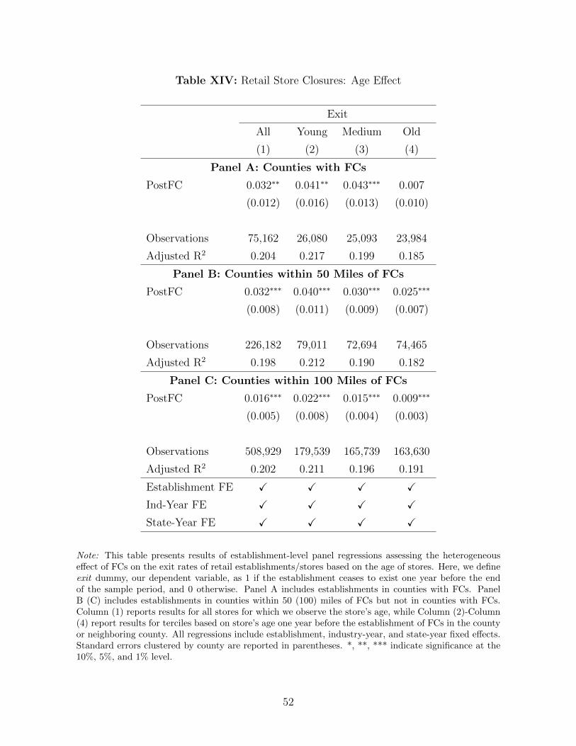
Table XIV: Retail Store Closures: Age Effect

Exit

All Young Medium Old

(1) (2) (3) (4)

Panel A: Counties with FCs

PostFC 0.032∗∗ 0.041∗∗ 0.043∗∗∗ 0.007

(0.012) (0.016) (0.013) (0.010)

Observations 75,162 26,080 25,093 23,984

Adjusted R2 0.204 0.217 0.199 0.185

Panel B: Counties within 50 Miles of FCs

PostFC 0.032∗∗∗ 0.040∗∗∗ 0.030∗∗∗ 0.025∗∗∗

(0.008) (0.011) (0.009) (0.007)

Observations 226,182 79,011 72,694 74,465

Adjusted R2 0.198 0.212 0.190 0.182

Panel C: Counties within 100 Miles of FCs

PostFC 0.016∗∗∗ 0.022∗∗∗ 0.015∗∗∗ 0.009∗∗∗

(0.005) (0.008) (0.004) (0.003)

Observations 508,929 179,539 165,739 163,630

Adjusted R2 0.202 0.211 0.196 0.191

Establishment FE X X X X

Ind-Year FE X X X X

State-Year FE X X X X

Note: This table presents results of establishment-level panel regressions assessing the heterogeneouseffect of FCs on the exit rates of retail establishments/stores based on the age of stores. Here, we defineexit dummy, our dependent variable, as 1 if the establishment ceases to exist one year before the endof the sample period, and 0 otherwise. Panel A includes establishments in counties with FCs. PanelB (C) includes establishments in counties within 50 (100) miles of FCs but not in counties with FCs.Column (1) reports results for all stores for which we observe the store’s age, while Column (2)-Column(4) report results for terciles based on store’s age one year before the establishment of FCs in the countyor neighboring county. All regressions include establishment, industry-year, and state-year fixed effects.Standard errors clustered by county are reported in parentheses. *, **, *** indicate significance at the10%, 5%, and 1% level.

52

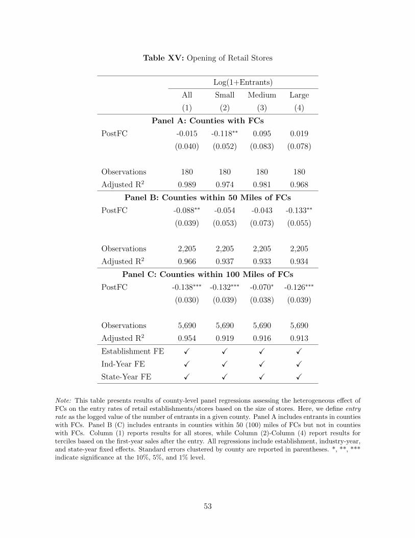
Table XV: Opening of Retail Stores

Log(1+Entrants)

All Small Medium Large

(1) (2) (3) (4)

Panel A: Counties with FCs

PostFC -0.015 -0.118∗∗ 0.095 0.019

(0.040) (0.052) (0.083) (0.078)

Observations 180 180 180 180

Adjusted R2 0.989 0.974 0.981 0.968

Panel B: Counties within 50 Miles of FCs

PostFC -0.088∗∗ -0.054 -0.043 -0.133∗∗

(0.039) (0.053) (0.073) (0.055)

Observations 2,205 2,205 2,205 2,205

Adjusted R2 0.966 0.937 0.933 0.934

Panel C: Counties within 100 Miles of FCs

PostFC -0.138∗∗∗ -0.132∗∗∗ -0.070∗ -0.126∗∗∗

(0.030) (0.039) (0.038) (0.039)

Observations 5,690 5,690 5,690 5,690

Adjusted R2 0.954 0.919 0.916 0.913

Establishment FE X X X X

Ind-Year FE X X X X

State-Year FE X X X X

Note: This table presents results of county-level panel regressions assessing the heterogeneous effect ofFCs on the entry rates of retail establishments/stores based on the size of stores. Here, we define entryrate as the logged value of the number of entrants in a given county. Panel A includes entrants in countieswith FCs. Panel B (C) includes entrants in counties within 50 (100) miles of FCs but not in countieswith FCs. Column (1) reports results for all stores, while Column (2)-Column (4) report results forterciles based on the first-year sales after the entry. All regressions include establishment, industry-year,and state-year fixed effects. Standard errors clustered by county are reported in parentheses. *, **, ***indicate significance at the 10%, 5%, and 1% level.

53

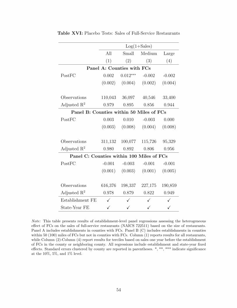
Table XVI: Placebo Tests: Sales of Full-Service Restaurants

Log(1+Sales)

All Small Medium Large

(1) (2) (3) (4)

Panel A: Counties with FCs

PostFC 0.002 0.012∗∗∗ -0.002 -0.002

(0.002) (0.004) (0.002) (0.004)

Observations 110,043 36,097 40,546 33,400

Adjusted R2 0.979 0.895 0.856 0.944

Panel B: Counties within 50 Miles of FCs

PostFC 0.003 0.010 -0.003 0.000

(0.003) (0.008) (0.004) (0.008)

Observations 311,132 100,077 115,726 95,329

Adjusted R2 0.980 0.892 0.806 0.956

Panel C: Counties within 100 Miles of FCs

PostFC -0.001 -0.003 -0.001 -0.001

(0.001) (0.003) (0.001) (0.005)

Observations 616,376 198,337 227,175 190,859

Adjusted R2 0.978 0.879 0.822 0.949

Establishment FE X X X X

State-Year FE X X X X

Note: This table presents results of establishment-level panel regressions assessing the heterogeneouseffect of FCs on the sales of full-service restaurants (NAICS 722511) based on the size of restaurants.Panel A includes establishments in counties with FCs. Panel B (C) includes establishments in countieswithin 50 (100) miles of FCs but not in counties with FCs. Column (1) reports results for all restaurants,while Column (2)-Column (4) report results for terciles based on sales one year before the establishmentof FCs in the county or neighboring county. All regressions include establishment and state-year fixedeffects. Standard errors clustered by county are reported in parentheses. *, **, *** indicate significanceat the 10%, 5%, and 1% level.

54

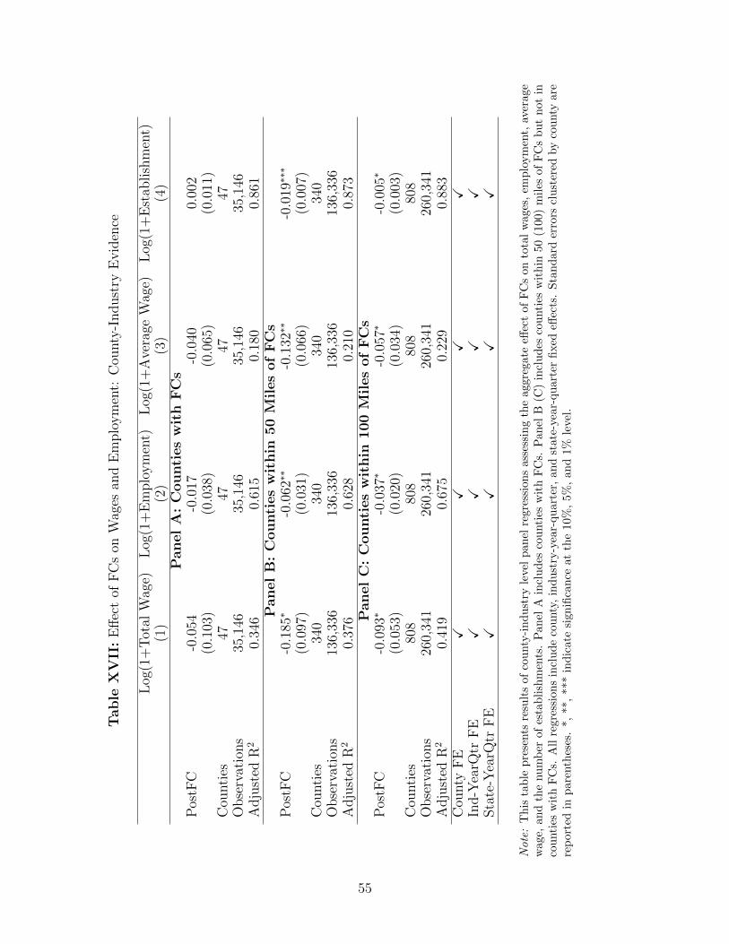
Table

XV

II:

Eff

ect

ofF

Cs

onW

ages

and

Em

plo

ym

ent:

Cou

nty

-Indust

ryE

vid

ence

Log

(1+

Tot

alW

age)

Log

(1+

Em

plo

ym

ent)

Log

(1+

Ave

rage

Wag

e)L

og(1

+E

stab

lish

men

t)(1

)(2

)(3

)(4

)P

anel

A:

Counti

es

wit

hF

Cs

Pos

tFC

-0.0

54-0

.017

-0.0

400.

002

(0.1

03)

(0.0

38)

(0.0

65)

(0.0

11)

Cou

nti

es47

4747

47O

bse

rvat

ions

35,1

4635

,146

35,1

4635

,146

Adju

sted

R2

0.34

60.

615

0.18

00.

861

Panel

B:

Counti

es

wit

hin

50

Mil

es

of

FC

sP

ostF

C-0

.185

∗-0

.062

∗∗-0

.132

∗∗-0

.019

∗∗∗

(0.0

97)

(0.0

31)

(0.0

66)

(0.0

07)

Cou

nti

es34

034

034

034

0O

bse

rvat

ions

136,

336

136,

336

136,

336

136,

336

Adju

sted

R2

0.37

60.

628

0.21

00.

873

Panel

C:

Counti

es

wit

hin

100

Mil

es

of

FC

sP

ostF

C-0

.093

∗-0

.037

∗-0

.057

∗-0

.005

∗

(0.0

53)

(0.0

20)

(0.0

34)

(0.0

03)

Cou

nti

es80

880

880

880

8O

bse

rvat

ions

260,

341

260,

341

260,

341

260,

341

Adju

sted

R2

0.41

90.

675

0.22

90.

883

Cou

nty

FE

XX

XX

Ind-Y

earQ

trF

EX

XX

XSta

te-Y

earQ

trF

EX

XX

X

Note:

Th

ista

ble

pre

sents

resu

lts

ofco

unty

-in

du

stry

leve

lp

an

elre

gre

ssio

ns

ass

essi

ng

the

aggre

gate

effec

tof

FC

son

tota

lw

ages

,em

plo

ym

ent,

aver

age

wag

e,an

dth

enu

mb

erof

esta

bli

shm

ents

.P

anel

Ain

clu

des

cou

nti

esw

ith

FC

s.P

an

elB

(C)

incl

ud

esco

unti

esw

ith

in50

(100)

mil

esof

FC

sb

ut

not

inco

unti

esw

ith

FC

s.A

llre

gres

sion

sin

clu

de

cou

nty

,in

dust

ry-y

ear-

qu

art

er,

an

dst

ate

-yea

r-qu

art

erfi

xed

effec

ts.

Sta

nd

ard

erro

rscl

ust

ered

by

cou

nty

are

rep

orte

din

par

enth

eses

.*,

**,

***

ind

icat

esi

gnifi

can

ceat

the

10%

,5%

,an

d1%

leve

l.

55

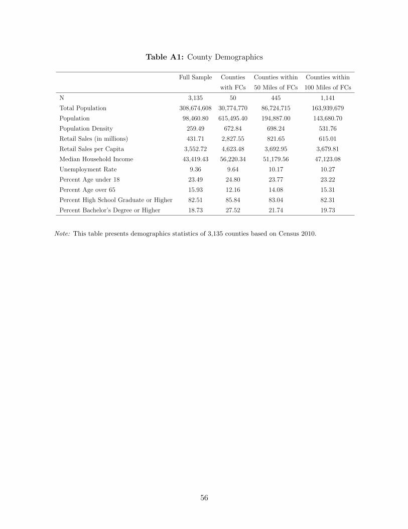
Table A1: County Demographics

Full Sample Counties Counties within Counties within

with FCs 50 Miles of FCs 100 Miles of FCs

N 3,135 50 445 1,141

Total Population 308,674,608 30,774,770 86,724,715 163,939,679

Population 98,460.80 615,495.40 194,887.00 143,680.70

Population Density 259.49 672.84 698.24 531.76

Retail Sales (in millions) 431.71 2,827.55 821.65 615.01

Retail Sales per Capita 3,552.72 4,623.48 3,692.95 3,679.81

Median Household Income 43,419.43 56,220.34 51,179.56 47,123.08

Unemployment Rate 9.36 9.64 10.17 10.27

Percent Age under 18 23.49 24.80 23.77 23.22

Percent Age over 65 15.93 12.16 14.08 15.31

Percent High School Graduate or Higher 82.51 85.84 83.04 82.31

Percent Bachelor’s Degree or Higher 18.73 27.52 21.74 19.73

Note: This table presents demographics statistics of 3,135 counties based on Census 2010.

56

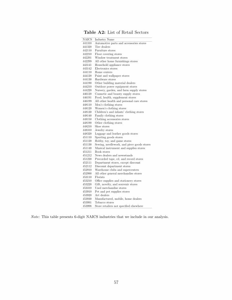
Table A2: List of Retail Sectors

NAICS Industry Name441310 Automotive parts and accessories stores441320 Tire dealers442110 Furniture stores442210 Floor covering stores442291 Window treatment stores442299 All other home furnishings stores443141 Household appliance stores443142 Electronics stores444110 Home centers444120 Paint and wallpaper stores444130 Hardware stores444190 Other building material dealers444210 Outdoor power equipment stores444220 Nursery, garden, and farm supply stores446120 Cosmetic and beauty supply stores446191 Food, health, supplement stores446199 All other health and personal care stores448110 Men’s clothing stores448120 Women’s clothing stores448130 Children’s and infants’ clothing stores448140 Family clothing stores448150 Clothing accessories stores448190 Other clothing stores448210 Shoe stores448310 Jewelry stores448320 Luggage and leather goods stores451110 Sporting goods stores451120 Hobby, toy, and game stores451130 Sewing, needlework, and piece goods stores451140 Musical instrument and supplies stores451211 Book stores451212 News dealers and newsstands451220 Precorded tape, cd, and record stores452111 Department stores, except discount452112 Discount department stores452910 Warehouse clubs and supercenters452990 All other general merchandise stores453110 Florists453210 Office supplies and stationery stores453220 Gift, novelty, and souvenir stores453310 Used merchandise stores453910 Pet and pet supplies stores453920 Art dealers453930 Manufactured, mobile, home dealers453991 Tobacco stores453998 Store retailers not specified elsewhere

Note: This table presents 6-digit NAICS industries that we include in our analysis.

57