The Danish pesticide leaching assessment programme: Site characterization and monitoring design

The Danish Pesticide

Leaching Assessment

Programme

Site Characterization and Monitoring

Design

Bo Lindhardt, Christian Abildtrup, Henrik Vosgerau, Preben Olsen, Søren Torp,

Bo V. Iversen, Jørgen Ole Jørgensen, Finn Plauborg, Per Rasmussen, and

Peter Gravesen.

Geological Survey of Denmark and GreenlandMinistry of Environment and Energy

Danish Institute of Agricultural SciencesMinistry of Food, Agriculture and Fisheries

National Environmental Research InstituteMinistry of Environment and Energy

Editor: Bo Lindhardt

Cover: Peter Moors

Lay-out and graphic production: Authors and Kristian Anker Rasmussen

Printed: September 2001

Price: DKK 500.00

ISBN 87-7871-094-4

Available from

Geological Survey of Denmark and Greenland

Thoravej 8, DK-2400 Copenhagen, Denmark

Phone: +45 38 14 20 00, fax +45 38 20 50, e-mail: [email protected]

www.geus.dk

© Danmarks og Grønlands Geologiske Undersøgelse, 2001

Tables of Contents

Preface

1. Introduction

1.1 Objectives of the programme 2

1.2 Schedule 2

1.3 Structure of the report 2

2. Site selection

2.1 Soil type 3

2.1.1 Areas with Quaternary clay 4

2.1.2 Areas with Quaternary sand 4

2.2 Climate 5

2.3 Hydrogeology 6

2.4 Site area 6

2.5 Site history 7

2.6 Site access 7

2.7 The six selected sites 8

3. Monitoring design

3.1 Groundwater monitoring 11

3.1.1 Piezometers 11

3.1.2 Vertical monitoring wells 14

3.1.3 Horizontal monitoring wells 14

3.2 Drainwater collection 16

3.3 Soil water sampling 18

3.4 Climate parameters 21

3.5 Monitoring device codes 22

4. Geological and pedological methods

4.1 Geological methods 23

4.1.1 Geological field work 23

4.1.2 Laboratoy analyses at GEUS 23

4.2 Pedological and soil hydrological methods 25

4.2.1 Pedological field work 25

4.2.2 Soil hydrology 28

4.3 Geophysical mapping 29

5. Site characterization

5.1 Site 1: Tylstrup 31

5.2 Site 2: Jyndevad 36

5.3 Site 3: Silstrup 38

5.4 Site 4: Estrup 43

5.5 Site 5: Faardrup 47

5.6 Site 6: Slaeggerup 52

5.7 Comparison of the sites 57

6. Pesticide selection 61

References 69

Annexes

Annexe 1. Site 1: Tylstrup A1-1

Annexe 2. Site 2: Jyndevad A2-1

Annexe 3. Site 3: Silstrup A3-1

Annexe 4. Site 4: Estrup A4-1

Annexe 5. Site 5: Faardrup A5-1

Annexe 6. Site 6: Slaeggerup A6-1

Preface

The Geological Survey of Denmark and Greenland (GEUS), the Danish Institute of Ag-

ricultural Sciences (DIAS), the National Environmental Research Institute (NERI), and

the Danish Environmental Protection Agency (DEPA) have been requested by the Dan-

ish Government to set up and run a programme to assess the risk of pesticides leaching

into surface waters and groundwater when applied in the prescribed manner. The pro-

gramme was designed and the test sites established during 1999. This report describes

the selected sites and the monitoring equipment installed.

The programme is managed by a project committee comprising:

Bo Lindhardt, GEUS

Jeanne Kjaer, GEUS (replaced Peter Gravesen as of 1 August 2000)

Svend Elsnab Olesen, DIAS

Arne Helweg, DIAS

Ruth Grant, NERI

Betty Bügel Mogensen, NERI

Christian Ammitsøe, Danish EPA

Christian Deibjerg Hansen, Danish EPA

Bo Lindhardt

August 2001

1

1. Introduction

There is a growing public concern in Denmark regarding pesticide contamination of

groundwater and surface waters. The Danish National Groundwater Monitoring Pro-

gramme (GRUMO) has revealed the presence of pesticides and their degradation prod-

ucts in approx. 30% of the monitored screens (GEUS, 2000). The increasing detection

of pesticides over the past 10 years has raised doubts as to the adequacy of the existing

approval procedure for pesticides. As the water sampled under the groundwater moni-

toring programme is usually more than 5 years old and often more than 20 years old, the

results are of limited value as regards evaluation of the present approval procedure.

EU and hence Danish assessment of the risk of pesticide leaching to the groundwater is

based mainly on data from laboratory or lysimeter studies. However, these types of data

assessment do not provide satisfactory characterization of the leaching that might occur

under actual field conditions. Soil (chemical properties and biological processes) and

hydrogeology can vary significantly within as well as between fields, and climate con-

ditions can vary during pesticide use. Furthermore, agricultural practice also varies be-

tween fields. Many of these parameters are not covered by laboratory or lysimeter stud-

ies as presently performed.

Laboratory and lysimeter studies provide little if any information on the inherent vari-

ability of the soil parameters affecting leaching. This is of particular importance for silty

and loamy soils, where preferential flow may occur. Field studies abroad have demon-

strated considerable transport of several pesticides to 1 m b.g.s. (below ground surface)

in loamy soils under conditions comparable with those in Denmark. The inclusion of

field studies, i.e. test plots exceeding 1 ha, in risk assessment of pesticide leaching to the

groundwater is considered an important improvement in risk assessment procedures.

The US-EPA has requested such field studies to support the registration of pesticides

suspected of potentially being able to leach to groundwater. Over the past decade, stud-

ies of more than 50 pesticides have been conducted. Based on this experience the US-

EPA has published a set of guidelines for field studies (US-EPA, 1998). In Europe, EU

Directive 91/414/EEC, annexe VI (Council Directive 97/57/EC of 22 September 1997)

enables field study results to be included in the risk assessments.

2

1.1 Objectives of the programme

The aim of the Pesticide Leaching Assessment Programme (PLAP) is to monitor

whether pesticides or their degradation products leach to groundwater under actual field

conditions when applied in the prescribed manner. The programme is designed such that

the findings can be evaluated in relation to the drinking water quality criterion, i.e. 0.1

←g/l.

The programme encompasses six test sites selected to represent the dominant soil types

and the climatic variation in Denmark. To provide early warning of unacceptable

leaching, the sites were selected where the groundwater was located 1-4 m below the

ground surface, thus ensuring a short response time. Pesticides are applied to the test

fields as part of routine agricultural practice and in accordance with the current regula-

tions, thereby enabling the occurrence of pesticides or their degradation products in the

groundwater downstream of the test field to be related to the current approval conditions

pertaining to the pesticides.

The programme will only include pesticides used in arable farming. Pesticides used in

forestry, fruit orchards and horticulture are not encompassed by the programme.

1.2 Schedule

Work on designing the programme started in August 1998. The six sites were selected

during 1999 and the equipment for sampling drainwater and groundwater was installed

the same year. This report presents the site characterization and the monitoring design of

each site. Monitoring was initiated between May 1999 and April 2000. The results will

be published in forthcoming reports.

1.3 Structure of the report

Chapter 2 provides a detailed description of the criteria used in selecting the test sites.

Chapter 3 describes the monitoring equipment and methods while Chapter 4 presents

the geological and pedological methods used to characterize the sites. Chapter 5 briefly

describes the six test sites with regard to instrumentation, pedology and geology. For a

more detailed characterization of each site the reader is referred to the accompanying

annexes. Finally, Chapter 6 presents the pesticides encompassed by the programme.

3

2. Site selection

Selection of the sites is critical with respect to ensuring that the results are generally

applicable and hence can be utilized in the pesticide approval procedures. The risk of

groundwater contamination by pesticides mainly depends on soil type, hydrogeology,

climate and agricultural practice. Site selection depends not only on these parameters,

but also on such factors as site access, i.e. permission from the owner, all year round

road access, access to electric power and, in the case of drained sites, an old and well

described tile drain system. This chapter presents the site selection criteria used and

briefly summarizes the six selected sites.

2.1 Soil type

The Danish EPA requires that pesticide testing is conducted under “worst case” condi-

tions. The test sites consequently need to be located on “vulnerable” soil types as re-

gards possible groundwater contamination. Coarse-textured sandy soils with a low or-

ganic matter content were previously considered to be among the most vulnerable soils.

Over the past decade, however, evidence has accumulated that pesticide leaching also

occurs on structured soils (Flury, 1996). The findings of the Danish National Ground-

water Monitoring Programme (GRUMO) also indicate that pesticides can leach to the

groundwater in regions dominated by structured soil types (GEUS, 2000). Only a few

studies have tried to compare the mass flux of pesticides from different soil types under

identical agricultural practices and climate conditions. At present, no information is

available concerning how to identify the most “vulnerable” soil types in Denmark as

regards leaching of pesticides to the groundwater. As suitable scientific documentation

on which to base selection of the most “vulnerable” soil types and hence the “worst

case” scenarios is lacking, we decided to select a number of sites representing the soil

types on which pesticides are most commonly applied in Denmark.

The geological composition of sediments down to 5-10 m b.g.s. in Denmark is known

from geological maps, profiles, excavations, well data and sometimes also geophysical

measurements. The composition of the uppermost metre of deposits is mainly known

from the systematic mapping of Quaternary deposits carried out by GEUS. This started

in 1888 and is still going on, about 80% of the Danish land area now having been

mapped. At deeper levels, knowledge of the geological deposits is mainly based on well

data. The deposits commonly vary considerably in grain size, internal structure and min-

4

eralogical and geochemical composition over short distances in both the vertical and

horizontal directions. In addition, glaciotectonic activity has commonly overprinted and

dislocated the deposits.

The map of Quaternary deposits shows that 40% of Denmark’s land area consists of clay

till, 28% of meltwater sand, 12% of Post-Glacial and Late-Glacial marine sand and aeo-

lin sand, 12% of Post-Glacial freshwater sand, 3% of sand till and 7% of different sub-

ordinate Quaternary deposits. Pre-Quaternary deposits account for less than 1% of

Denmark’s surface. In considerable areas, however, Cretaceous and Danian limestone

and Tertiary clay are reached within a depth of 5 m b.g.s. In view of the above-

mentioned distribution it was decided that the sites should be located in both areas with

Quaternary clay and areas with Quaternary sand.

2.1.1 Areas with Quaternary clay

Clayey sediments occurring near the ground surface are dominated by clay till deposits.

These characteristically consist of a very unsorted sediment with a clay content exceed-

ing 12–14%. The till deposits were formed in contact with ice, either laid down beneath

the ice (lodgement till) or deposited from the surface of the ice as it melted (ablation and

flow tills). Lodgement tills are more consolidated than ablation and flow tills due to the

heavy burden of the ice during their deposition. Clay tills are generally chararacterized

by containing fractures formed by glaciotectonic forces or by desiccation and freeze-

thaw processes. Subsurface Pre-Quaternary deposits may considerably affect the compo-

sition of the overlying till. For instance, the clay or chalk content may be very high in

the case of a clay till deposited by a glacier that has passed an area with exposed Terti-

ary clay or Cretaceous chalk. The till deposits which form the ground surface in Den-

mark were generally deposited by ice advances that occurred 20–14,000 BP during the

Late Weichselian Period. In western Jutland, however, an older glacial landscape occurs

as hill islands in the Weichselian outwash plains. The meltwater and till deposits that

form part of this landscape were deposited during the Saalian period 140,000 BP, and

hence have been exposed to weathering, erosion and soil-forming processes for a very

long period.

2.1.2 Areas with Quaternary sand

The meltwater sediments were transported and deposited by meltwater from glaciers.

Grain size thus diminishes from meltwater gravel to meltwater sand with increasing

distance from the former ice front. They are subdivided into glacial meltwater sedi-

ments, which are sometimes deformed by subsequent ice advances, and Late-Glacial

extramarginal meltwater sediments, which have not been overridden by glaciers. The

5

extramarginal meltwater sediments form large outwash plains east of the Main Station-

ary Line marking the westernmost extension of the Weichselian ice sheet in Jutland.

Post-Glacial and Late-Glacial marine sand was formed when land areas were flooded

due to an interplay between isostatic uplift and eustatic sea level rise caused by melting

of local and global icecaps, respectively. Today these sediments form raised seafloor

plains in the landscape as a result of subsequent isostatic uplift.

Aeolian sediments were deposited in the Post-glacial period and consist of well sorted,

fine-grained sand deposited as dunes, mainly in coastal regions, and as coversand when

deposited inland.

Freshwater sand was mainly deposited along streams and in lakes during the Post-

glacial period.

2.2 Climate

Together with soil type, one of the most important parameters controlling pesticide

leaching is the precipitation. The most common way to express the regional variation in

precipitation is by the annual mean. The annual mean precipitation in Denmark during

the period 1961–90 was 712 mm/year, varying from 550 mm/year in the Store Bælt re-

gion to 900 mm/year in the southern part of Jutland (Frich et.al., 1997). The inter-annual

variation in annual mean precipitation at individual single sites varies by a factor two.

Thus while the annual mean precipitation ranged from 456 to 744 mm/year during the

period 1988–97 in the Roskilde region, it ranged from 557 to 1,032 mm/year in the Jyn-

devad region.

The variation in pesticide leaching cannot be ascribed to the variation in annual mean

precipitation alone. The transport of pesticides through unsaturated soil is controlled by

a complex interaction between the degree of saturation and the intensity of the precipi-

tation. This interaction is not a useful parameter for selecting sites. Only the annual

mean precipitation is of practical usefulness when selecting site location.

Other climate parameters that affect pesticide leaching, e.g. temperature and evapora-

tion, do not vary much in Denmark. Thus only the variation in precipitation has been

taken into account when selecting the sites.

The sites may not be further than 8 km away from an automatic climate station in order

to ensure access to additional good quality climate data and historical time series. Pre-

6

cipitation is also measured at the sites along with soil temperature and soil water con-

tent.

2.3 Hydrogeology

The depth of the water table is an important site selection factor. In order to ensure a

rapid response in the groundwater downstream of the test field and to facilitate sam-

pling, the water table must be as near to the surface as possible and no deeper than 5 m

b.g.s. The Danish EPA defines groundwater as water that leaves the root zone 1 m b.g.s.

In large parts of Denmark, the water table is less than a few metres below the surface.

The sites must be located inside the infiltration area and have a downward gradient. To

ensure a stable response in the monitoring well, a steady hydraulic gradient is required.

Sites located within the radius of influence of irrigation or production wells have thus

been as far as possible avoided. Where this is not possible it is necessary to obtain in-

formation on the production from the wells.

The infiltration of water and hence leaching of pesticides is influenced by surface run-

off. To minimize surface runoff the selected sites have a low topographic slope – less

than 2% slope in general.

The sites with structured soil have to be drained and the tile drain system must be well

known and only cover the test field. Moreover, the tile drains must be more than 10

years olds so that the overlying soil has had time to consolidate, thereby avoiding artifi-

cial infiltration to the drain system. The base flow must be as low as possible to avoid

dilution of the response. In order to facilitate sampling of the drainwater it is important

that the drainage system feeds into a single outlet.

2.4 Site area

The size of the test field is crucial. On one hand it needs to be sufficiently large to ade-

quately cover the variation in soil structure, particularly on clay soils where preferential

flow is expected to form the key route for pesticide transport down through the unsatu-

rated zone. On the other hand, the area must not be too large because the variation in the

soil structure would then complicate interpretation of the results. That sampling costs

increase with increasing test field size also points to the selection of as small a site as

possible. The test field should only encompass single soil series, with a small spatial

variability in the soil parameters. Test sites between 1 and 4 ha are assumed to be an

7

acceptable compromise. The US-EPA guidelines for prospective groundwater monitor-

ing studies requires test sites of equal size (US-EPA, 1998).

To eliminate artificial flow patterns it is important to select sites with undisturbed soil.

Areas where sampling by drilling has taken place or where excavation has been per-

formed should thus be avoided.

2.5 Site history

The previous crop rotation on the site is expected to influence the fate of the pesticide.

The test field should previously have been subjected to conventional agricultural prac-

tices as regards crop rotation and soil tillage, thus excluding the use of fields with

minimal or conservation tillage, organic farming, horticulture and set-aside.

We prefer fields that have been cultivated as one parcel with the same crop within re-

cent years, and exclude sites that have been used for plot experiments or have been dis-

turbed by excavation, drilling or deep soil sampling.

Pesticide use at the sites must have been recorded for at least the previous 5-year period.

2.6 Site access

Pesticide leaching studies are typically conducted over a 2–3 year period for each appli-

cation. As the present programme will run for a period of up to 10 years, sites could

only be included if a long-term lease was possible.

For practical reasons there must be good road access to the sites all year round to enable

sampling. Moreover, in order to obviate the necessity to establish an on-site power sup-

ply to run the sampling equipment, mains electricity had to be within reasonable reach.

The sites also had to be located within approx. 10 km of a state experimental farm such

that the pesticides and tracers could easily be applied by trained personnel from the state

experimental farms. However, standard agricultural operations such as soil tillage,

sowing and harvesting could be done by the landowner when deemed appropriate.

8

2.7 The six selected sites

The programme encompasses six sites. This number of sites is a compromise balancing

monitoring intensity with the number of different soil types represented by the pro-

gramme. Two of the sites are located on sandy soil and four on clayey soil. The key data

for each of the six sites are presented in Table 2.1. The location of each site is shown in

Figure 2.1.

Three of the sites (1 sandy and 2 clayey) are in regions with relatively high precipitation,

while the other three are in drier regions. A brief description of each site is given in

Chapter 5.

Table 2.1. Key data for the six selected sites encompassed by the Danish Pesticide Leach-ing Assessment Programme.Name Tylstrup Jyndevad Silstrup Estrup Faardrup Slaeggerup

Location Brønder-

slev

Tinglev Thisted Vejen Slagelse Roskilde

Crop

1999 Potatoes

2000 Springbarley

Winter rye

Fodderbeet

Springbarley

Winterwheat

Springbarley

2001 Winterrye

Maize Springbarley

Peas Sugar beet

Peas

2002 Springbarley

Winterwheat

Winterwheat

Springbarley

Winterwheat

B x L, m 70 x 166 135 x 184 91 x 185 120 x 105 160 x 150 165 x 130Area, ha 1.1 2.4 1.7 1.3 2.3 2.2

Soil type Finesand

Coarsesand

Clayey till Clayey till Clayey till Clayey till

Deposited by Saltwater Meltwater Glacier Glacier Glacier Glacier

Tile drain No No Yes Yes Yes Yes

Precipitation,

mm/year1)

668 858 866 862 558 585

1) Yearly normal based on a time series from 1961-90

9

100 km

3. Silstrup

4. Estrup

2. Jyndevad

1. Tylstrup

5. Faardrup

6. Slaeggerup

Clay till

Sandy soil

Figure 2.1. Location of the six test sites in Denmark.

11

3. Monitoring design

Characterization and instrumentation of the sites was carried out in an integrated manner

with the soil cores from the monitoring well boreholes being used to develop a concep-

tual hydrogeology model for the sites. The different types of devices installed at each

site are described here.

The monitoring equipment used and aspects monitored include:

• Piezometers – potentiometric pressure of the groundwater

• Vertical and horizontal monitoring wells – sampling of groundwater

• Suction cups – water samples from unsaturated soil

• Automatic ISCO samplers – sampling of drainwater

• Weather stations – precipitation

• TDR-probes – soil water content

• Pt-100 sensors – soil temperature

• Pressure sensors – barometric pressure

Figure 3.1 shows the typical lay-out of monitoring devices at a site.

To avoid any artificial leaching of pesticides, drilling and excavation have not been car-

ried out inside the plot used for pesticide treatment. All installations and soil sampling

deeper than 20 cm b.g.s. are restricted to a buffer zone around the treated plot.

3.1 Groundwater monitoring

3.1.1 Piezometers

Four multiple-level piezometers each with three separate piezometer screens have been

installed at each site. The casings and the screens are made of the same material and

have the same dimensions. High-density polyethylene (HDPE) pipes from Filter Jensen

(DK) with an outside diameter of 63 mm and a wall thickness of 5.8 mm were used. The

screens are 50 cm long and contain two 0.5 mm aperture slits per cm.

12

The three screens of each piezometer are installed in the same borehole. The diameter of

the borehole is 152 mm (6"). In the clay soils drilling was carried out with a solid stem

auger while a bailer technique was used below the water table in the sandy soils. Surface

casing was used when necessary. For filter packing we used Grejs No. 2 (0.7–1.2 mm)

(Grejsdalens Filterværk, DK). A filter pack seal of at least 100 cm bentonite (Pellerts,

QS, Cebro, NL) was installed approx. 10 cm above each screen (Figure 3.2). Each nest

of multiple-level piezometers is protected at the surface by a 0.6 m dia. concrete ring

closed by a padlocked metal cover.

Tile-drain

Vertical monitoringwells

PiezometersRain gauge

Automatic drainwater samplers

TDR, Pt-100 andsuction cups

Horizontal wells

Buffer zone

Groundwaterflow

Figure 3.1. Typical lay-out of monitoring devices at a tile-drained site.

13

The lower screen in each nest is located between 11.5 and 12 m b.g.s. The top screen is

located such that the water table is expected to be permanently above the screen. At the

clay sites the screens are placed in the most sandy horizon.

The water level is measured either manually by using a “water level indicator” or con-

tinuously using one of three different transducer-logger systems. Every time samples are

collected, the water level in all the piezometers is measured manually. In the piezometer

closest to the “shed” the water level is measured on-line every hour using a differential

pressure transducer (Druck, Limited, UK) connected to a Campbell datalogger. At the

sandy sites, the water level is monitored in one screen. At the clay sites two Druck

1 m

2 m

Filter 1

Filter 3

Filter 2

Filter 4

Piezometers Vertical monitoring wells

Bentonite

Backfill

Clay pelletsFilter sand

6”

6”

Figure 3.2. Construction of a multiple-level piezometer and monitoring well at a clay

till site.

14

transducers are installed – one in the upper screen and another in the lower screen. The

water level in the piezometer diagonally opposite the corner where the shed is located

was initially measured continuously every hour using an Orphimedes-logger (OTT, D).

In early spring 2000, this system was exchanged for a D-diver (RoTek a/s, DK), which

is a pressure transducer and a data-logger. As the D-diver does not take into account

changes in barometric pressure, the raw data have to be corrected using the barometric

pressure measured at each site.

3.1.2 Vertical monitoring wells

For sampling groundwater, seven vertical monitoring wells were installed at each site.

The drilling techniques and the materials used for the casings and screens are the same

as for the piezometers. Sorption of pesticides to the HDPE piping is expected to be in-

significant (Fetter, 1999; US-EPA, 1998). The pipe material was tested for release of

any compounds that could contaminate the water samples and no evidence was found of

any contamination that might interfere with analysis of the 39 different pesticides in-

cluded in the Danish Groundwater Monitoring Programme (GEUS, 2000).

Each monitoring well consists of four screens. The length of each screen is 100 cm. The

screens are placed so that they cover the upper 4 metres of the groundwater. The top of

the upper screen is placed above the highest seasonal water table. To avoid vertical

movement of water along the casing, each screen is installed in its own borehole. To

optimize sealing, clay pellets (Tonkugeln, Duranit VFF; D) were used as back-fill.

Monitoring well construction is shown in Figure 3.2.

For water sampling, a Whale pump (GP9216, 13 l/min, 72 watt, 12 V, RoTek a/s, DK)

was permanently installed in each screen connected to a PE-tube (6 x 1 mm or 10 x 1

mm, RoTek a/s, DK).

One monitoring well is located upstream of the test field, while the other six are distrib-

uted downstream of the test field (Figure 3.1).

3.1.3 Horizontal monitoring wells

The water flow transporting the pesticides is difficult to monitor in areas with clayey till

because of the effect of vertical preferential flow and the frequent occurrence of sandy

lenses, which can cause lateral flow. To overcome these difficulties a number of hori-

zontal monitoring screens have been installed approx. 3.5 m b.g.s. inside the treatment

plot at the four sites on clayey till.

15

3.5

m.b

.g.s.

18 m 1 m

Outlet

Buffer zoneBuffer zone

“Rimming” and placing the casing

Drilling by flushing with water

Bentonite seal

Outlet tubes

Inner pipe

One filter section

A

B

C

Backfill

Tile-drain

Complete installation

Figure 3.3 Installation of horizontal monitoring wells and a section of the horizontalscreen.

16

The horizontal screens are installed by drilling from the buffer zone on one side of the

treated plot to the buffer zone on the opposite side without causing any disturbance to

the topsoil inside the plot. The technique used for drilling these horizontal boreholes is

well known from installing power cables or pipelines beneath roads, etc. The drilling rig

is placed on the surface and drilling performed in two steps: Firstly, forward drilling by

a water flushing technique and secondly, reaming whereby the rod is drawn back. The

diameter of the final boreholes is 200 mm. In the first step the drilling rod can be steered

by changing the position of the rod head, which is continuously monitored at the surface

by a radio signal. The sediments are released by flushing with water and transported out

of the borehole by the water flow. The diameter of the borehole made by forward drill-

ing is 110 mm. To reduce the water pressure, a mud pit is excavated at the entrance to

the borehole just outside the test field in the buffer zone (see Figure 3.3A). When the

rod has traversed the treated plot and penetrated an excavation on the other side a

reamer is installed on the rod together with a 160 mm o.d. casing. The screens with

bentonite packers are placed inside the casing and the casing then drawn into the bore-

hole at the same time as the “rimming” takes place (Figure 3.3B). At the specific posi-

tions the screens are fixed by retaining them with a wire while the casing is drawn out of

the borehole. The complete installation procedure is shown in Figure 3.3C.

The screens are 18 m long with an outer diameter of 125 mm and a wall thickness of 5.8

mm. The screens have two 0.5 mm aperture slits per cm. Two tubes are installed at each

screen. The outer diameter of the inside pipe is 63 mm (Figure 3.3) while tubes are 10

mm in diameter with wall thickness of 1 mm. The screens are made of HDPE and the

tubes of PE. Three individual screens are installed in each borehole separated by 1 m

bentonite seals.

Sampling from the screens is performed with a peristaltic pump on the surface.

3.2. Drainwater collection

The four clayey till sites are located in areas with an existing tile drainage system. As a

criterion for selecting the sites the drainage system had to be systematically described

and easily isolated to represent a well-defined monitoring area. At all four sites it was

necessary to cut off some drainpipes and/or to install additional pipes to ensure a de-

fined catchment area. The modifications made at each site are described in the accom-

panying Annexes 1–6.

17

In order to enable the measurement of drainage runoff and the collection of drainwater

samples a concrete monitoring well was established at the outlet of each drainage sys-

tem. The wells are 1.25 m in diameter and 2–3 m deep.

The monitoring wells are constructed with a sharp-crested V-notch weir (Thomson

weir) made of 5 mm galvanized iron plate. The Thomson weir is the most exact profile

for measuring runoff with a large variation in flow rate (Bos, 1976). A 30 V-notch an-

gle was chosen as a compromise between high precision at relatively low flow rates and

low sensitivity to blockage of the notch. The height of the notches is not less than 30

cm.

Campbell data-logger

Thomson weir

30 V-notch�Drain pipe in

Drain pipe out

Timeprop.

Flowprop.

Pressure transducer

Inlets to ISCOsamplers

1.25 m

2-3 m

ISCO Samplers

From the sideFrom ahead

Figure 3.4. Drainwater monitoring well with Thomson weir and water sampler.

18

Table 3.1. Infiltration per ha vs. flow in the drainage system.

Height above the

Thomson weir, cm

Flow in drain, Q

(l/s)

Infiltration, q

mm/ha/day

5 0.23 2

10 1.2 10

20 6.8 59

30 19 164

A Thomson weir requires a free fall from the weir notch of at least 25 cm. The water

level above the V-notch is monitored using a pressure transducer (Druck PDCR 1830,

Druck Limited, UK). The transducer is mounted in a stainless steel tube (length 1,100

mm, diameter 21.5 mm) fixed to the wall of the well by means of a stainless steel clamp

(Figure 3.4). To protect the transducer from turbulent water at high flow rates, it is

placed in a special chamber behind the weir and as far away from the drain inlet as pos-

sible (Figure 3.4). The pressure transducer is connected to the central Campbell datalog-

ger.

The water samples are collected using ISCO 6700 (Isco, Inc. US) samplers equipped

with eight 1,800 ml glass bottles (boron silicate), teflon suction tubes and intakes of

stainless steel. The intakes are placed a few centimetres into the inlet of the drainpipe so

as to ensure sampling of flowing drainwater and particulate matter. Two samplers are

used at each site: One for time-proportional sampling and one for flow-proportional

sampling. The time-proportional sampler is equipped with refrigerated bottles such that

the water samples can be collected over a 7-day period. The flow-proportional sampler

is only activated during storm events and sampling is carried out for 1–2 days depending

on the intensity of the event.

The monitoring wells are each located inside a shed so as to protect the equipment from

the weather. Two electrical heaters in each shed prevent the temperature from dropping

below 5C.

3.3 Soil water sampling

Soil water in the unsaturated zone is under tension, and hence cannot flow into a well as

groundwater does. Monitoring of soil water in the unsaturated zone thus requires the use

of suction cups, etc.

19

Treated area

Buffer zoneShed withsample bottles

Clusters of suction cups, TDR and Pt-100

Approx. 20 m

Approx. 4 m

EFTE tubes

Treated area Buffer zone

Suctioncup

Clay pellets

Bentonite

EFTE tubes

Approx. 2 mExcavation

Suction cups4 cups at 2 depths

TDR3 probes at 6 depths

Soil temperature1 probe at 5 depths

1 m

1 m

2 m

2 m

Approx.4 m 0.8 m

0.25

0.6

0.91.1

1.9

2.1

A

B

C

Figure 3.5. A) Location of suction cups, TDR and soil temperature probes, B) a crosssection showing the installation of the suction cups, and C) a plan view of an excavationwall indicating the location of the suction cups, TDR and soil temperature probes.

20

A total of 16 suction cups have been installed at two locations at each site – one on each

side of the test field about 20 meters from the downslope corner (Figure 3.5A).

At each location, four suction cups are installed at a depth of 1 m b.g.s. and four at a

depths of 2 m b.g.s. (Figure 3.5B/C). The horizontal distance between suction cups in-

stalled at the same depth is 1 m while that between suction cups installed at different

depths is 0.5 m.

The suction cups were installed from two excavation pits at the edge of each test field

via holes drilled obliquely to the desired depth. This procedure ensures that the soil di-

rectly above the suction cups remains undisturbed.

The suction cups installed at a depth of 1 m are located at a horizontal distance of 2 m

from the edge of the test field while the suction cups installed at a depth of 2 m are lo-

cated at a horizontal distance of 2.5 meters from the edge of the field. The installation

holes were drilled from 0.5 m b.g.s. in the case of the suction cups installed at a depth of

1 m and from 1 m b.g.s. in the case of those installed 2 m b.g.s.

The installation holes were drilled with a 50 mm air-driven hand auger to the desired

length minus 20 cm. The final 20 cm of the installation holes were completed using a 21

mm steel rod corresponding to the diameter of the suction cup.

100 ml of a thick slurry of water and silica flour was poured to the bottom of the hole

just before installation of the suction cup. Immediately after installation of the suction

cup a further 100 ml of the slurry was poured into the installation hole, which was then

sealed with 20 cm of clay pellets before being back-filled with bentonite pellets.

Each suction cup is connected to the sampling bottle via a single length of PTFE tubing.

From the excavation pit to the shed the PTFE tubes run through a protective tube buried

in a 70 cm deep trench. The sampling bottles are located in a refrigerator in the shed.

The soil water is extracted using a continuous vacuum technique.

The suction cups used are PRENART SUPER QUARTZ (Prenart, DK) consisting of

porous PTFE mixed with quartz. The soil water sampler is 21 mm in diameter and 95

mm in length with 2 micron pores. The tubes used consist of 1/8" x 2.0 mm PTFE tub-

ing. The sampling bottles are 1 or 2 litre glass bottles. All fittings that come into contact

with water are made of stainless steel.

21

3.4 Climate parameters

An automated monitoring system has been installed at each site for measurement of

precipitation, barometric pressure, soil temperature, soil water content and soil water

pressure. At the four sites on clayey till, the system also controls two drain water sam-

pling devices (Section 3.2).

The automated system consists of various items of hardware and sensors and commer-

cially available software tools in which dedicated software codes have been imple-

mented. The central unit is a Campbell CR10X 2M datalogger (Campbell Sci, UK).

User communication from office PC to this datalogger is established via modem using

fixed telephone lines or GSM phone transmission. The data are collected automatically

every night.

Precipitation

Precipitation is measured on site with a tipping bucket rain gauge (Type 1518Wilh.

Lambrecht, BmbH, D). The gauge is accurate to 0.1 mm and is well suited for measur-

ing high precipitation intensity. Sampling is carried out every minute and hourly values

are stored.

Soil moisture

Soil moisture is measured using a CR10X-controlled Time Domain Reflectometry

(TDR)-system. The central unit in the TDR-system is the cable tester from Tektronix

1502C (Tektronix Inc., Beaverton, OR, USA). The soil water probes are developed at

Research Centre Foulum and consist of a 40 m coaxial cable (Mikkelsen Electronic A/S,

DK) connected through a solid plastic box to three 30 cm steel rods spaced about 2 cm

apart. The accuracy of the soil water measurements is around �1 vol %.

Soil water content is measured in two profiles at each site at the depths of 0.25, 0.6, 0.9,

1.1, 1.9 and 2.1 m (Figure 3.5C), with three replicate probes at each depth. Soil water

content is measured and stored every hour.

Soil temperature

Soil temperature is measured with platinum resistance thermometers (Pt-100, length 10

mm and diameter 5 mm). The accuracy of the measurements is �0.1°C. Soil temperature

is measured in two profiles at each site with one sensor at each of the following depths:

0.1, 0.25, 0.6, 1.0 and 2.0 m (Figure 3.5C). The temperature is measured and stored

hourly.

22

Barometric pressure

The barometric pressure is measured with a pressure sensor (PTB101B, Vaisala, SF)

with an accuracy of �2 mB. Measurements are taken and stored hourly.

3.5 Monitoring device codes

To ensure unique identification of all samples collected in this programme, all sampling

points are described by a code that includes the site identification, the type of sampling

device, and the number of sample points in each device. The code system is illustrated

in the box above.

By way of example, a vertical monitoring screen on the Tylstrup site will have the code

1.M4.3, indicating screen number 3 in vertical monitoring well (M) number 4 at site

number 1.

The screens in the vertical monitoring wells and the piezometers are coded with in-

creasing numerical value from the surface and downward.

X.XX.X

Site number1. Tylstrup2. Jyndevad3. Silstrup4. Estrup5. Faardrup6. Slaeggerup

Device typeP : PiezometerM: Vertical monitoring wellH: Horizontal monitoring wellD: Tile-drainS: Suction cup

Device number1..., e.g. monitoringwell number at a site.

Device index1...3, e.g. screennumber in a monitoring well.

23

4. Geological and pedological methods

4.1 Geological methods

4.1.1 Geological field work

The initial field work at the sites included drilling of one to four shallow boreholes with

a hand auger in order to determine whether the desired geology was present. Subse-

quently, four 12 to 23 m deep wells each fitted with three piezometers were drilled to

monitor the potential head of the shallow groundwater flow and determine the direction

of flow. Once the direction of flow had been determined, seven monitoring well clusters

were established – six downstream of the test field and one upstream.

A geologist in the field supervised all drilling and the geology was described in the field

in accordance with Larsen et al. (1995). Samples were taken for each 0.5 m or at least

one sample from each described layer. All well data and the geological description are

stored in the GEUS water well database JUPITER.

Test pits

At the four clay till sites (Silstrup, Estrup, Faardrup and Slaeggerup) a 5 m deep 10 x 10

m test pit was excavated in the buffer zone with profiles perpendicular to each other at

three levels: 0.5–2.0 m, 2.0–3.5 m and 3.5–5.0 m. This test pit structure enabled all

fracture orientations to be observed. The profiles were described according to Klint and

Gravesen (1999). The test pits were used for the following tests and investigations: field

vane tests, fracture description and characterization, fabric analysis and lithological de-

scription. Samples were collected for grain size analysis, total organic carbon (TOC)

and CaCO3 content, clay mineral analysis and exotic stone counts.

4.1.2 Laboratory analyses at GEUS

Total organic carbon (TOC)

TOC content was determined as follows: 300–500 mg of sample was treated with 5–6%

H2S03 to remove carbonate minerals and then combusted in a LECO CS 200.

24

CaCO3

Each bulk sample was gently crushed sufficiently to pass a 2 mm sieve. 25 ml 0.5 M

hydrochloride acid and demineralized water was then added and the sample heated to

boiling point for 20 minutes. Thereafter the suspension was titrated with 0.5 M sodium

hydroxide using phenolphthalein as indicator.

Grain size

Grain sizes larger than 0.063 mm were determined by sieving according to DS 405.9 but

with a ½ phi sieve column.

Material smaller than 0.063 mm was sieved through a 0.1 mm sieve cloth and the mate-

rial larger than 0.1 mm dried, treated with 50 ml 0.005 M Na4P2O7 x 10 H2O and centri-

fuged. After 12 hours of shaking the sample was measured using a Micromeritics Sedi-

Graph 5100.

Permeability

The plug dimensions were measured with a calliper and the plug then mounted in a spe-

cial Hassler core holder at a confining sleeve pressure of 1.75 bar. The required fluid

and fluid upstream pressure of 0.2–1.5 bar was delivered by a constant flow rate pump.

At least one pore volume of liquid was allowed to flow through the sample before the

measurements were initiated. The flow rate was measured volumetrically over a period

ranging from a few hours to more than one day.

Porosity and grain density

The porosity was measured in cleaned and dried samples by subtraction of the measured

grain volume and the measured bulk volume. The grain volume was determined using

the helium technique (Boyle’s law) applying a double-chambered helium porosimeter

with a digital readout. The bulk volume was measured by submersion of the plug in a

mercury bath using Archimedes’ principle. Grain density was calculated from the grain

volume measurement and the weight of the cleaned and dried sample.

Porosity by weight loss

The porosity of loosely consolidated sediments, e.g. till samples that are saturated to

100% with a liquid, can be analysed by drying at 110C and recording the weight loss.

The weight loss was recalculated to a liquid volume equal to the pore volume. The sam-

ple bulk volume was determined from calliper measurements of the saturated sample

before drying.

25

Clay mineralogical analysis

The samples were gently crushed to pass a 2 mm sieve and treated with sodium acetate

at a pH of 5 to remove carbonates. The sand and silt fraction was then removed by elu-

triation and centrifugation, and the 2-30 µm fraction and clay fraction < 2 µm were

separated in a particle size centrifuge. The clay fraction was saturated with Mg2+ and K+

prior to X-ray diffraction analysis.

Oriented specimens were prepared by the pipette method and the following specimens

analysed:

Mg2+ – saturated, air dry.

Mg2+ – saturated, glycolate.

K+ – saturated, air dry.

K+ – saturated , heated to 300°C.

X-ray diffraction was carried out with Co-K∼ radiation, ϒ-filter and pulse

height selection.

Fine gravel analysis (Ehlers, 1978)

4.2 Pedological methods

4.2.1 Pedological field work

Excavation and description of soil profiles

Two or three soil profiles were excavated at each site to a depth of approx. 1.6 m using a

backhoe. Major excavations performed by GEUS and used for geological site descrip-

tions were also used to describe the upper 1.6 m of the soil profile.

Pedological description of all identified soil horizons was carried out in accordance with

Madsen and Jensen (1988). Field reports from the sites included detailed maps showing

the succession of identified and described soil horizons. Profile descriptions, photo-

graphs and drawings are presented in the annexes.

Soil samples from every identified horizon were collected for laboratory analysis. About

10 litres of bulk soil from each horizon were dried and stored at DIAS. The soil samples

were analysed at the DIAS. A detailed description of the laboratory analysis methods

used can be found in Hansen and Sørensen (1996). The most important methods and

procedures are briefly summarized in Table 4.2.

26

Table 4.2. Summary of methods and procedures used in the laboratory analyses of soilsamples.Parameter Description

Soil texture Particle size analysis subdivided the soil samples into the following classes: clay <2 µm,

silt 2–20 µm, coarse silt 20–63 µm, fine sand 63–125 µm and 125–200 µm, medium

sand 200–500 µm, and coarse sand 500–2,000 µm.

TOC The total organic carbon (TOC) content was determined using dry combustion. Soil

samples containing significant amounts of calcium carbonate (exceeding 1%) were also

analysed for CaCO3 content.

pH pH was measured following suspension of the soil in 0.01 M CaCl2.

Fe and Al Fe and Al were extracted using an ammonium oxalate solution and determined by

atomic absorption spectrophotometry.

Total-P Phosphorous content was determined spectrophotometrically following destruction of

the soil by perchloric acid-sulphuric acid.

Total-N The soil sample was combusted in an atmosphere of pure oxygen at 900°C. Water and

CO2 were removed and the nitrogen oxides were reduced to free nitrogen, which was

then measured in a chemical conductivity cell.

Exchangeable

cations

Exchangeable cations were extracted using ammonium acetate buffered at a pH of 7.0.

Ca and Mg were determined using atomic absorption spectrophotometry. Na and K were

determined by flame emission. Exchangeable hydrogen ions were determined by titra-

tion to equilibrium in a 0.06 M-nitrophenol solution.

CEC CEC was calculated as the sum of cations.

The soil profiles were classified both according to the Danish system (Madsen and Jen-

sen, 1985) and the USDA Soil Taxonomy (Soil Survey Staff, 1999). Nomenclature for

textural classes in this investigation follows the Danish system, illustrated in Figure 4.1.

The description and the analysis results from all the profiles have been stored in the

DIAS soil profile database (Den Danske Jordprofil Database – DDJD (The Danish Soil

Profile Data Base)).

Soil core descriptions

The soil core samples for description were retrieved to a depth of 1 m b.g.s. using a

hand auger or until 1.2 m b.g.s. by using a hydraulic soil auger provided by DIAS. Soil

horizons and soil texture have been described for approx. every 25 metres along the

edge of the test field. The position of each described soil core was geo-referenced using

DGPS to an accuracy of 0.2 m. Soil cores retrieved with the hand auger were deter-

mined using local fix points.

27

Silt

Silt loamLoam

Sandy Loam

Sandy clay

loam

Loasand

Clay loam Silty clay

loam

Silty

claySandy

Clay

Clay

100 90 80 70 60 50 40 30 20 10

9

8

7

60

0

0

0

50

4

3

2

1

0

0

0

09

8

7

6

50

40

30

20

1

0

0

0

0

0

100 90 80 70 60 50 40 30 20 10

9

8

7

60

0

0

0

50

4

3

2

1

0

0

0

09

8

7

6

50

40

30

20

1

0

0

0

0

0

Jyndevad

Tylstrup

Silstrup

Estrup

Faardrup

Slaeggerup

Clay Silt

Sand

Clay Silt

Sand

Very heavy

clay

Sandy heavy

clay

Heavy

clay

Silty heavy clay

Silty clay

Clayey sandy silt

Clayey

silt

Sandy

clay

Silt

Sandy silt

Clayey silty sand

Silty sand1 2 1214

13

43

5

7 8 15 16

10 11 17

18

6

3 clayey sand

5 Very clayey sand

USDA soil texture classification

Danish soil texture classification

Sand

Very clayey silty sand

Clay

Sandmy

B

A

Figure 4.1. A) USDA (Soil Survey Staff, 1999) and B) Danish (Madsen and Jensen,1988) soil classification triangel. Samples from the A-horizon taken at the soil profileson each of the six fields.

28

Description of excavated trenches

Trenches excavated in order to establish the cut-of drainage pipes were used for map-

ping soil horizons and for determination of soil texture. Soil horizons and soil texture

were described for every 25 m along the 0.8–1.6 m deep trenches.

Total carbon mapping

The topsoil (0–25 cm) at each site was sampled in a 20 m grid. Nine soil samples were

collected at each grid point – one point exactly at the grid point and the other eight

points arranged symmetrically around the grid point at a distance of 1 m. The nine sam-

ples were then pooled and the total organic carbon content determined at the Depart-

ment of Analytical Chemistry, DIAS (Tabatabai and Bremner, 1970).

4.2.2 Soil hydrology

At all six sites, soil cores were taken from within three levels of the soil profiles corre-

sponding to the A-, B-, and C-horizons. Five 6,280 cm3 soil cores (large cores) and nine

100 cm3 soil cores (small cores) were collected from each horizon. The nine small cores

were divided into three groups with each group being collected near and around one of

the large cores. To collect the large cores a large sampling cylinder was forced into the

soil by means of a hydraulic press mounted on a tractor. To collect the small cores a

small sampling cylinder was forced into the soil with a hammer using a special flange.

All samples were protected from evaporation and stored at 2-5°C until analysis.

Analysis of large cores

In the laboratory the large cores were placed on a ceramic plate and saturated with water

from below. The samples were then drained to a soil water potential of -50 cm. H2O and

air permeability were measured using a portable air permeameter (Iversen et al., 2001).

The samples were then left to re-saturate and the near-saturated hydraulic conductivity

was measured using a drip infiltrometer (van den Elsen et al., 1999). This works auto-

matically and measures the hydraulic conductivity in the soil under steady-state water

flow conditions at different soil water potentials. The soil column was placed on a sand-

box and five ceramic cups connected to transducers were placed in the soil column.

When steady-state water flow was reached, a measurement was conducted and the

measurement continued at lower water potential. Upon completion of the drip infil-

trometer measurements the samples were re-saturated and the saturated hydraulic con-

ductivity measured using the constant-head method (Klute and Dirksen, 1986). Near-

saturated hydraulic conductivity and air permeability were only measured on three out of

five samples, whereas saturated hydraulic conductivity was measured on all five sam-

ples.

29

Analysis of small cores

Small soil cores were placed on top of a sandbox and saturated with water from below.

Soil water characteristic were determined by draining the soil samples successively to

soil water potentials of -10, -16, -50, -100, -160, and -1,000 cm H2O (pF 1, pF 1.2, pF

1.7, pF 2, pF 2.2, and pF 3.0) using a sandbox for potentials from -10 to -100 cm H2O

and a ceramic plate for potentials from -160 to -1,000 cm H2O. Soil water characteristics

were also determined at a soil water potential of -15,850 cm H2O (pF 4.2) after the soil

had been ground and sieved through a 2 mm sieve (Klute, 1986). Air permeability was

measured at a soil water potential of –50 cm H2O using the same device as for the large

soil cores. After the soil water characteristic had been determined the samples were re-

saturated and the saturated hydraulic conductivity measured using the constant-head

method (Klute and Dirksen, 1986). Finally, the soil samples were oven-dried at 105°C

for 24 hours and weighed in order to determine the dry weight.

All analyses were carried out at the Department of Crop Physiology and Soil Science,

DIAS except for the pF 4.2 analysis, which was carried out at the Department of Ana-

lytical Chemistry, DIAS.

4.3 Geophysical mapping

Geo-electrical mapping of the sites was performed using an EM-38 sensor and a CM-

031 ground conductivity meter. Both instruments measure the apparent specific conduc-

tivity by electromagnetic induction (Durlesser, 1999). The electromagnetic conductivity

of the soil is a function of such factors as the content of salts, clay and water (Rhoades

and Corwin, 1981).

EM-38 mapping

Simplified maps generated by means of the EM-38 sensor delineate soil types according

to their clay content (Nehmdahl, 2000). The measurement unit is millisiemens per metre

(mS/m) and the penetration depth of the sensor is 1–1.5 m.

The mapping system developed at DIAS consists of a 4-WD motorcycle equipped with

a GPS receiver and data-logger, pulling a sledge on which the EM-38 is mounted to-

gether with a GPS antenna.

Data from the EM 38 and GPS were stored simultaneously with a frequency of 1 meas-

urement per second while navigating in parallel lines separated by a distance of approx.

10 m. Measurements were made at approx. 10 m intervals and used to produce interpo-

lated maps of the soil electrical conductivity.

30

Conductivity meter (CM-031)

The electrical conductivity from 1 to 6 m b.g.s. was mapped at five of the six sites using

a CM-031 ground conductivity meter (Geofyzika, Czech). A local 10 m by 20 m grid

was established at the site and measurements made with both vertical and horizontal

dipole orientations. The vertical dipole orientation corresponds to a penetration of 5.5–6

m whereas the horizontal dipole orientation corresponds to a penetration of approx. 1 m.

The data were automatically stored in a HP palmtop during field work.

Note that the resistivity values at depths down to 1 m were measured with EM 38

whereas the measurements at 2.5–3 m b.g.s. and 5–6 m b.g.s. were made using the CM-

031. The two instruments are operated at different heights above the ground surface.

Ground-penetrating radar (GPR)

To detect any larger sand or gravel lenses or other geological anomalies and obtain in-

formation about internal structures such as bedding plane, the area was mapped with

ground-penetrating radar in a 20 to 30 m grid using a 100 MHz antenna. The GPR map-

ping was performed by FAXE Kalk A/S, DK.

31

5. Site characterization

In this chapter each of the six sites is described briefly in respect to instrumentation,

pedology, and geology. For a detailed characterisation of the sites the reader is referred

to the relevant Annexe.

5.1 Site 1: Tylstrup

This test field is situated at Tylstrup in northern Jutland. It covers an area of 1.08 ha and

the width of the buffer zone is approx. 2 m towards the northeastern, 3 m towards the

southeastern, 22 m towards the southwestern and 4.5 m towards the northeastern. Wind-

breaks run along the western and eastern side of the buffer zone and a road runs along

the northern side of the site. All installations are shown in Figure 5.1.

Instrumentation

Four wells each containing three piezometers were installed in the buffer zone. Each

cluster consists of three 0.5 m long screens distributed over the depth interval 4.5–12 m

b.g.s. An additional two piezometers consisting of ¾" electroplated pipes were also in-

stalled in the buffer zone and two were installed approx. 150 m south of the test field.

The groundwater table fluctuates between 3 and 4 m b.g.s. Based on the groundwater

potential in the piezometers in spring 1999 it was concluded that the direction of

groundwater flow is towards west-southwest. The monitoring wells were therefore

placed such that 6 of the 7 monitoring well clusters were located downstream of the test

field. Each cluster contained four separate 1 m long screens covering approx. the depth

interval 2–6 m b.g.s. on the western side of the site and 1.6–5.6 m b.g.s on the eastern

side.

Two groups of suction cups, TDR-probes and Pt-100 sensors were installed at the

southwestern corner of the site, i.e. the downstream corner of the test field in relation to

the direction of the groundwater flow.

Geology

The Tylstrup site is located on Late-Glacial fine-grained marine sand deposited in a

shallow Arctic sea – the Yoldia Sea – approx. 15,000 BP. The area has subsequently

32

been subject to isostatic uplift and the Late-Glacial marine deposits are now found as

one in a series of raised seafloor terraces.

The pattern of sediment distribution at the site indicates the presence of more fine-

grained material, i.e. silt and clay layers, in the northern end of the field. The geophysi-

cal mapping is in good accordance with the well data and the field can be described as

homogeneous. The pedological profiles at the site are classified as Typibrunsols. A

geological-pedological model has been established on outcrop, borehole and geophysi-

cal data. The four units are presented below. A borehole croos section from the site is

illustrated in Figure 5.2.

N

0 50 m

%

%

%

%

%

%

#

#

#

#$Z

P3

P6P4

P7

P8

#

#

#

M1

M2

M3

M4

M5

M6

M7

S1

S2 P5

Suction cups, TDR andPt-100

% Piezometer

# Monitoring well

Shed

$Z Rain Gauge

Buffer Zone

Groundwaterflow

Figure 5.1. Sketch of the Tylstrup field showing the test and buffer zones, location ofinstallations and the direction of the groundwater flow.

33

Figure 5.2 NE-SW cross section based on wells at the Tylstrup site. The location of thewells is shown in Figure 5.1.

34

Unit 1: Topsoil. 0–0.4 m b.g.s.

The very dark greyish brown sandy topsoil (loamy sand) contains humus (1.7–2.3%

TOC), a varying content of burrows and roots, and is an Ap horizon. The material is

noncalcareous. On the lee side of the windbreaks, Ap2 horizons are present, formed as a

result of eolian sediment transport. The saturated hydraulic conductivity ranges from 10-

6–10-5 m/s.

Unit 2: Oxidized noncalcareous weathered fine-grained silty sand. 0.4–1.6 m b.g.s.

This unit is a yellowish brown, brownish yellow or dark olive brown silty sand classi-

fied as a Bv and a Bc horizon with wormcasts and roots to a depth of 1.6 m. The TOC

content is approx. 0.3–1.5%. Placic horizons and hydromorphic characters are also pres-

ent in the unit. Sedimentary structures are obscured as a result of soil formation proc-

esses. In the northern half of the field the unit can be expected to contain some silt and

clay layers. The saturated hydraulic conductivity is approx. 10-5 m/s.

Unit 3a: Oxidized noncalcareous silty sand. 1.6–approx. 4 m b.g.s.

The silty sand in the unit is yellow or light yellowish brown, fine grained and silty. In

outcrops it contains a variety of sedimentary structures such as lamination cross-bedding

and erosive surfaces. The TOC content is less than 0.1%. In the top part of this unit the

saturated hydraulic conductivity ranges from 10-5–10-4m/s.

Unit 3b: Oxidized noncalcareous silty sand with clay and silt layers. 1.6–approx. 4 m

b.g.s.

This unit is confined to the northern half of the field. It consists of interbedded sand, silt

and clay layers. The sand in the unit is yellow or light yellowish brown and the clay-silt

layers are light olive brown. The different lithologies often appear as heterolithic beds,

i.e. thin alternating layers. Silt layers typically have a lateral extension of approx. 10 m.

The TOC content is less than 0.1%.

Unit 4: Oxidized weakly calcareous silty sand. 4–12 m b.g.s.

This unit consists of light yellowish brown silty sand with very few silt or clay layers.

The CaCO3 content is approx. 1.5–2.0% and TOC content is less than 0.1%.

Regional aquifer

The regional aquifer in the area is an extensive 20–30 m thick meltwater sand and

gravel unit of Weichselian age located approx. 3–20 m b.g.s.

35

0 50 m

N

#

#

#

##

%

%

%

%$Z$Z$Z

P8

P11

P10

S2

S1

P9

#

#

M7

M6M5

M4

M3

M2

M1


% Piezometer

# Monitoring well

Shed

$Z Rain Gauge

Buffer Zone

Groundwaterflow

Figure 5.3. Sketch of the Jyndevad site showing the test and buffer zones, location ofinstallations and the direction of the groundwater flow.

36

5.2 Site 2: Jyndevad

This test field is situated at Store Jyndevad in southern Jutland. It covers an area of 2.39

ha and the width of the buffer zone is 24 m towards the north, 16 m towards the west, 14

m towards the south and 3 m towards the east. A windbreak borders the field to the east.

All installations are shown in Figure 5.3.

Instrumentation

Four wells each containing three piezometers were installed in each corner of the site in

the buffer zone. Each cluster consists of three 0.5 m long screens distributed over the

depth interval 3.4–11.5 m b.g.s. An additional seven piezometers were installed at a

distance of up to 900 m from the site. The groundwater table fluctuates between 1 and 2

m b.g.s. Based on the groundwater potential in the piezometers in summer 1999 the di-

rection of groundwater flow was concluded to be west-northwest. The monitoring well

clusters were therefore placed such that 6 of the 7 clusters were located downstream of

the test field. Each cluster contained four separate 1 m long screens covering the depth

interval 0.6–5.4 m b.g.s. at the western side of the site and 1.6–5.6 m b.g.s at the eastern

side.


northwestern corner of the site, which is the downstream corner in relation to the direc-

tion of the groundwater flow.

Geology

The site is located on a Late Weichselian outwash plain west of the Main Stationary

Line marking the westernmost extension of the Weichselian ice sheet. The outwash

plain consists of meltwater sand and gravel locally draped by Post-Glacial eolian sand.

Meltwater sand and gravel with a few silt and clay layers dominate the site. The melt-

water sand unit in the area is at least 25 m thick and the Pre-Quaternary surface is lo-

cated at a depth of approx. 30–40 m.

The three soil profiles at the site have been classified as Typipodsols. equivalent to a

Humic Psammentic Dystrudept.

The geophysical mapping is in good accordance with the well data and the field can be

described as very homogeneous. A geological-pedological model has been established

on outcrop, well and geophysical data. The four units are described below and cross

sections are illustrated in Figure 5.4.

37

Figure 5.4. Cross sections based on wells at the Jyndevad site. The location of the wellsis shown in Figure 5.3.

38

Unit 1: Top soil. 0–0.3 m b.g.s

The black topsoil consists of sand with a content of TOC at 1.5–2.5%, and is an Ap ho-

rizon. The saturated hydraulic conductivity ranges from 10-5–10-4 m/s.

Unit 2: Weathered noncalcareous meltwater sand. 0.3–1.2 m b.g.s.

The black to yellowish brown unit consists of sand with small amounts of clay and silt.

It contains three horizons: Bhs, Bs and BC. Remains of sedimentary structures such as

cross-bedding and lamination can be observed. The TOC content is 0.25–0.75% and the

saturated hydraulic conductivity is approx. 10-4 m/s.

Unit 3: Noncalcareous meltwater sand. 1.2–5.5 m b.g.s.

This unit is dominated by alternating beds of fine to medium-sized meltwater sand and

medium- to coarse-grained meltwater sand. A few thin clay silt layers are present as

well. Sedimentary structures such as cross-bedding and ripple lamination can be ob-

served in the sand. Clay and silt account for less than 10% of the sand matrix. TOC

content is lower than 0.2%. The saturated hydraulic conductivity ranges from 10-4–10-3

m/s.

Unit 4: Unweathered weakly calcareous meltwater sand. 5.5–>12 m b.g.s.

This unit is similar to unit 3, but has a CaCO3 content of 0–4.5%. The transition from

oxidized to reduced conditions as indicated by colour changes is in good agreement with

water well data from 10–12 m b.g.s.

Other deposits

In monitoring wells M3, M4 and M6, one or several clay and silt layer beds and stringer

are present. In M3 the stringers are present to such an extent that the lithology takes on a

heterolithic character.

Regional aquifer

The regional aquifer consists of extra-marginal meltwater deposits and to some extent

more deep-lying Miocene quartz sand deposits.

5.3 Site 3: Silstrup

This test field is situated at Silstrup south of Thisted in northwestern Jutland. It covers

an area of 1.69 ha and the width of the buffer zone is 18 m towards the west and east, 5

m towards the south (where a small road acts as an additional buffer zone) and more

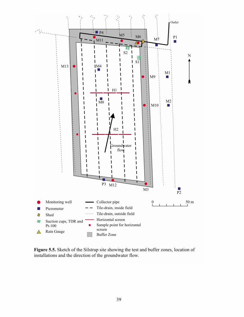
than 10 m wide towards the north. All installations are shown in Figure 5.5.

39

0 50 m10 m

N

$Z$Z %

%

%

%

%

%

%

%

%

#

##

#

#

#

#

P4

M4S1

S2

M7P1

M1

M8

H1

H2

P3

0 50 m

#

#

M11

M13

M9

M5 M6

M10

M12M3

P2

M2

Outlet


% Piezometer

# Monitoring well

Shed

$Z Rain Gauge

Tile-drain, inside field

Tile-drain, outside field

Collector pipe

Sample point for horizontalscreen

Buffer Zone

Horizontal screen

Groundwaterflow

Figure 5.5. Sketch of the Silstrup site showing the test and buffer zones, location ofinstallations and the direction of the groundwater flow.

40

Instrumentation


cluster consists of three 0.5 m long screens distributed over the depth interval 2.0–12.0

m b.g.s. Based on the groundwater potential in the piezometers in summer 1999 it was

concluded that the direction of the groundwater flow is towards the north. The moni-

toring wells were therefore placed such that 6 of the 7 clusters were located downstream

of the test field. Each cluster contained four separate 1 m long screens covering the

depth interval 1.5–5.5 m b.g.s.

The drainage system at the site was installed in the 1960s. The design of the drainage

system in the test field was simple, consisting of 5 parallel field drains running from

south to north connected to two transverse collector drains at the northern end. All ex-

isting drainpipes are clayware. The lateral drains are 6.5 cm i.d. while the main drains

are 8 cm and 10 cm i.d. The laterals appeared to have an envelope of seashells (mussels)

to improve permeability.

The monitoring chamber was placed in the northeastern corner of the field. The two

easternmost pipes exited towards the west, where a new 98 m PE pipe had to be laid

along the northern boundary of the field to lead the water from the northwestern corner

to the measuring chamber in the northeastern corner.


northeastern corner of the site, their positions being determined by that of the drainwater

monitoring chamber.

Two 58 m long horizontal sampling wells H1 and H2 were also installed at Silstrup.

Each consisted of three 18 m screen sections separated by 1 m bentonite seals. The first

screens (H1.1 and H2.1) of both wells are situated within a lateral distance of 17 m from

the edge of the test field.

The wells were drilled perpendicular to the edge of the field with the screens 3.5 m

b.g.s. According to the drilling company, part of H2 follows a “pavement” probably

comprised of a clay till rich in stones and boulders.

Geology

The Silstrup site is located north of the Main Stationary Line of the Weichselian Glacia-

tion. Weichselian glacial clay till deposits dominate the site and only few thin bodies of

41

13

M13

Figure 5.6. A geological model for the Silstrup site.

42

meltwater sand are present. Dislocated Oligocene clay and silt are present in the till

along the southern rim of the test field. The site is situated in an area of glaciotectonic

thrust faults and the coastal cliff east of the site contains dislocated Palaeocene and Oli-

gocene deposits deformed by glaciers from the NNE and N.

The geophysical mapping is in good accordance with the well data and the field can be

described as homogeneous.

A geological-pedological model comprised of the four units described below has been

established on outcrop and borehole data and is illustrated in Figure 5.6.


The dark grey brown to black sandy clayey topsoil (sandy clay loam/sandy loam) con-

tains humus (1.9-2.4 % TOC) and numerous burrows and roots. The unit is also heavily

fractured by vertical desiccation fractures. It is an Ap horizon and the material is non-

calcareous. The saturated hydraulic conductivity ranged from 10-6–10-4 m/s.

Unit 2: Noncalcareous oxidized clay till. 0.5–1.3m b.g.s.

The oxidized yellow brown clay till is penetrated by roots and burrows mainly in the

upper part. The till is generally noncalcareous but some spots at the site are calcareous.

Several horizontal-subhorizontal fractures are present. The till is weathered and the B

horizon consists of Bv and Bt with clay illuviation in the lower part. The saturated hy-

draulic conductivity ranges from approx. 10-5–10-4 m/s.

Unit 3: Calcareous oxidized clay till. 1.3–3.5 m b.g.s.

The brown and light yellow brown clay till is oxidized and calcareous (C- horizon). The

till contains small vertical and subvertical fractures which decreases in amount with

increasing depth. Additional sparse horizontal to subhorizontal fractures occur in this

unit. Dislocated Oligocene clay and silt are included along the southern rim of the site.

Saturated hydraulic conductivity values range from 10-7–10-5 m/s

Unit 4: Calcareous reduced clay till. 3.5–13 m b.g.s.

The olive grey clay till is calcareous and contains chalk and chert gravel. Only very few

vertical fractures exist at this depth while horizontal and subhorizontal fractures are

more abundant.

Other deposits

At the southern end of the field, dislocated Oligocene clay and silt layers are found in-

terbedded in the clay till. Since the clast fabric in the clay till indicates a deformation

from the north, it is likely that the dislocated Oligocene layers strike approx. 90 and dip

43

towards the north. The clay content of these layers ranges from 20–30% and the silt

content from 40–80%. The TOC content is 1.0–2.1%.

Regional aquifer

The sparse well data available for the area reflect the fact that there is no primary aquifer

below the Silstrup site. However, the chalk is found at a depth of at least 100 m.

5.4 Site 4: Estrup

This test field is situated west of Vejen in central Jutland. It covers an area of 1.26 ha

and the width of the buffer zone is 10 m towards the north and west, 5 m towards the

south (where the railroad is) and 15 m towards the east. All installations are shown in

Figure 5.7.

Instrumentation



m b.g.s. Based on the groundwater potential in the piezometers in autumn 1999 it was

concluded that the direction of groundwater flow is to the northeast. The monitoring

wells were therefore placed such that 6 of the 7 clusters were located downstream of the

test field. Each cluster contained four separate 1 m long screens covering the depth in-

terval 1.5–5.5 m b.g.s.

The drainage system was established in 1965. It is thought to be constructed of 6.5 cm

drains. To prevent water outside the test field from entering the drainpipes in the test

field, a cut-off drain was installed along the south and east boundary of the site. The

monitoring chamber was placed in the northeastern corner of the site. A 85 m long pipe

running 1–2 m from the edge of the ditch collected discharge from the two 8 cm pipes

that originally led to the ditch. Water from the main drainage system was conveyed to

the monitoring chamber by a 5 m long pipe. The two branches join as a T-junction right

outside the chamber.



monitoring chamber.

Due to the prevailing geological conditions, only one of two planned horizontal wells

were installed. Three 18 m screen sections and four 1 m bentonite seals were installed

44

3.5 m b.g.s. beneath the northeastern corner (H1). The samples are collected from the

southern end of the well. A second attempt was made to drill a horizontal well from a

position 7 m west of M2 to 13 m north of M6, but the borehole had to be abandoned

after 15 m of drilling in sand.

Geology

The Estrup site is located west of the Main Stationary Line of the Weichselian Glacia-

tion and the clay till that dominates the site is therefore Saalian. The site has a complex

geological structure comprising a clay till core with deposits of different age and com-

#

%

%

%

%

$Z$Z

0 50 m

P2

S2

S1

P3

P4

P1

#

#

#

#

#

#

#

M2

M3

M4

M5

M6

M7

M1

H1

N

Outlet


% Piezometer

# Monitoring well

Shed

$Z Rain Gauge



Collector pipe


Buffer Zone

Horizontal screen

Groundwaterflow

Figure 5.7. Sketch of the Estrup site showing the test and buffer zones, location of in-stallations and the direction of the groundwater flow.

45

position (Figure 5.8). At the southern rim of the site, shallow Post-Glacial peat is de-

positedupon a meltwater clay above the till. In the northwestern corner, a Saalian melt-

water sand basin with intercalation of till and silt layers is present. Along the eastern rim

of the area there is a small meltwater sand body. In the northeastern corner, a small la-

custrine basin filled with clay and gyttja rests on the clay till. The age of the deposits

could be Weichselian Interstadial or Eemian Interglacial. Small bodies of black mica-

( )

Figure 5.8. A geological model for the Estrup site.

46

ceous clay (not shown on Figure 5.8) with a high content of organic material are consid-

ered to be glacially dislocated Miocene sediments.

The soil profiles developed in the clay till at the site are classified as Pseudogleytypiles-

sive, whereas the soil profiles in the meltwater sand are classified as Lessive Pseu-

dogleytypipodsol.

The Estrup site is heterogeneous with different lithologies of Saalian, Weichselian and

Post-Glacial ages. The long exposure of the sediments to weathering during the glacial-

interglacial-glacial cycle has resulted in pedological development of acidification, de-

calcification and transport of fines and organic matter resulting in leached upper hori-

zons.

The clay and sand till body is the most important lithology as regards the geological

model. It is difficult to incorporate all the lithologies in one single model, and a geologi-

cal-pedological clay till model has therefore been established and relationships to the

other sediments are mentioned. The four units of the model are described below and a

conceptual 3-D model is illustrated in Figure 5.8.

Unit 1: Topsoil. 0-0.4 m b.g.s.

The topsoil consists of very dark greyish brown clay and clayey sand (sandy loam) with

a TOC content between 1.7 and 7.3%. It is an Ap horizon and is noncalcareous. The

saturated hydraulic conductivity ranges from 10-6–10-4 m/s.

Unit 2: Noncalcareous clay till. 0.4–1.0 to 4.0 m b.g.s.

The yellow brown clay till is noncalcareous and oxidized. Root channels reach down to

a depth of 2 m in this zone and occur together with randomly oriented small desiccation

fractures. From 2.0 to 4.0 m the fractures are still randomly oriented, but systems of

small vertical fractures and horizontal-subhorizontal fractures also occur. A few large

fractures are found. The till is heavily weathered and has an upper BE-horizon with clay

evaluation , a middle Bt horizon with clay and Fe and Mn oxide illuviation, and a lower

C horizon. The saturated hydraulic conductivity is 10-7–10-5 m/s. Other sediment bodies

present at the site are in contact with unit 2 and may influence the upper part of the hy-

draulic system of the Estrup site.

Unit 3: Non calcareous/calcareous clay till. 4–=approx. 12 m b.g.s.

The light yellow to brown grey sandy clay till is oxidized. The calcareous content varies

through the unit due to the occurrence of chalk rafts. Abundant large vertical fractures

and horizontal fractures occur and form a three-dimensional pattern. The saturated hy-

47

draulic conductivity ranges from 10-9–10-7 m/s. The meltwater sand bodies are in con-

tact with unit 3.

Unit 4: Calcareous clay and sand till. >12 m b.g.s.

This unit consists of alternating reduced calcareous grey clay till and sandy till beds with

some sand veins.

Other deposits

In addition to the deposits included in the clay till model, the site also includes the fol-

lowing:

Noncalcareous Saalian meltwater sand in the northeastern corner of the site. A gla-

cial raft of Miocene micaceous clay with a TOC content of 10% is found in the

southeastern corner at a depth of approx. 2 m.

South of the site 2 m of Post-Glacial peat was found with a TOC content of 50% and

no CaCO3. East of the site there is a 5 m thick glaciofluvial sand body with a clay

till bed. Northwest of the site there is a 7 m thick sequence of glaciofluvial sand with

clay till and silt beds.

Regional aquifer

The regional aquifer is located approx. 20 m b.g.s. and consists of meltwater sand.

5.5 Site 5: Faardrup

This test field is situated at Faardrup south of Slagelse on Zealand. It covers an area of

2.33 ha and the width of the buffer zone is >11 m towards the north, 12 m towards the

west (where the road adds another 4 m to the buffer zone), 17 m towards the east and

>11 m towards the south. All installations are shown in Figure 5.9.

Instrumentation

Four clusters of piezometers were installed in each corner of the test field, in the buffer

zone. Each cluster consisted of three 0.5 m long screens distributed over the depth inter-

val 1.5–13.2 m b.g.s. Based on the ground water potential in the piezometers during

summer 1999 it was concluded that the direction of groundwater flow was towards the

west. The monitoring wells were then placed such that 6 of the 7 monitoring well

48

#

#

#

#

#

#

%

%

%

%

$Z

P2

P3

H2

H1

P4

P1

#

#

M2

M3

M4

M5

M6

M7

M1

S1

S2

NOutlet

0 50 mSuction cups, TDR andPt-100

% Piezometer

# Monitoring well

Shed

$Z Rain Gauge



Collector pipe


Buffer Zone

Horizontal screen

Groundwaterflow

Figure 5.9. Sketch of the Faardrup site showing the test and buffer zones, location ofinstallations and the direction of the groundwater flow.

49

clusters were located downstream of the test field. Each cluster contained four separate

1 m screens covering the depth interval 1.5–5.5 m b.g.s.

The drainage system at Faardrup was installed in 1944. The map from 1944 shows a

traditional systematic drainage system. The drainage water from the test field and the

adjacent fields is collected in a 15 cm main drain that runs along the western side of the

area. The drainage system in the test field is a “herringbone system” with a collector

drain that runs down westwards from the hills to the east, crosses the middle of the field

and ends in the 15 cm main drain. All the drainpipes are clayware – 5.5 cm i.d. laterals

and 6.5 cm and 10 cm i.d. collector drains. The monitoring chamber was placed in the

northwestern corner of the site.

To isolate the test field drainage system, two cut-off drainpipes were installed. South of

the test field there is a smaller, independent drainage system which also exited at the top

end of the 15 cm main in the southwestern corner of the experimental field. This system

was disconnected at this point and the water lead downstream via a new watertight pipe

installed along the western boundary, parallel to the old main. A second cut-off drain

made of perforated, corrugated pipes with an envelope of gravel was installed to the

north and the east of the test field to prevent water from running into the test field from

its upstream side. All the existing drains intersected were closed off with a brick to-

wards the experimental field, and their upstream parts were connected to the new drain-

pipe via a T-junction.


northwestern corner of the site, their positions being determined by that of the drainwa-

ter monitoring chamber.

Two horizontal sampling wells were installed at Faardrup. Both wells were planned to

consist of five 18 m screens separated by 1 m long bentonite seals, total length 96 m,

including a 1 m bentonite seal at each end. Due to technical difficulties, however, H1

only consists of three 18 m long screens separated by 1 m bentonite seals.

H1 was drilled under the northeastern corner of the field. The overall drilled length is

160 m, of which 120 m lie beneath the test field. The screens are positioned from 3.35

to 3.70 m b.g.s. The samples are collected from the northern end of H1. Well H2 inter-

sects the southwestern corner of the field. The overall drilled length is 158 m, of which

110 m lies beneath the test field. The screens are positioned from 3.2 to 3.7 m b.g.s. The

samples are collected from the northern end of H2.

50

Figure 5.10. A geological model for the Faardurp site.

51

Geology

The Faardrup site is dominated by Weichselian clay till deposits more than 18 m thick

and overlying a regional meltwater sand aquifer. The till deposits are covered by a

clayey topsoil 0.3-0.4 m thick. The upper part of the till is classified as sandy-clayey till

as the clay content is about 12%. This part is heavily weathered, bioturbated and frac-

tured. The underlying clay till consists of an upper oxidized unit down to 4.1 m b.g.s.

and below a reduced unit. Borehole information shows that the clay till body contains

small channels or basins consisting of meltwater clay and sand (Figure 5.10).

The two of the soil profiles developed in the more or less clay-rich till are classified as

Pseudogleytypilessive and one as Degralessive.

The geophysical data are in accordance with the well and outcrop data and the test field

can be described as relatively homogenous representing the variability of the till plain. A

geological-pedological model for the clay till has been established consisting of the 4

units described below. A conceptual 3-D model is illustrated in Figure 5.10. The melt-

water sand and clay layers are not included in the model.


The dark brown topsoil consists of clay and sand (loam/sandy loam) with TOC content

between 1.2-1.8% and is an Ap horizon, of sandy loam. The material is noncalcareous.

The deposits contain numerous wormholes and root channels. Saturated hydraulic con-

ductivity ranges from 10-6–10-3 m/s.

Unit 2: Noncalcareous sandy clay till. 1.1–1.8 m b.g.s.

The yellow brown sandy-clayey till with sand lenses is oxidized and noncalcareous.

Numerous burrows and roots are present but decrease in number with increasing depth.

Vertical fractures (desiccation cracks) occur through the whole unit. The till is heavily

weathered, often with an upper BE horizon showing eluviation of clay and a lower Bvt

horizon showing illuviation of clay and Fe and Mn oxides. The saturated hydraulic con-

ductivity of the till is relatively high (compared to till deposits), ranging from 10-5–10-3

m/s.

Unit 3: Calcareous clay till. 2–4.2 m b.g.s.

The olive brown and yellow clay till is oxidized and calcareous. Few deep roots pene-

trate down into this unit. The unit is dominated by a network of fractures: Numerous

horizontal to subhorizontal fractures, many small fractures and few large fractures

penetrating down to at least 5 m b.g.s., i.e. into Unit 4. The saturated hydraulic conduc-

tivity ranges from 10-6–10-5 m/s in the upper part (1.5m) and 10-9 m/s in the lower part.

52

Unit 4: Reduced clay till. 4–>18 m b.g.s.

The olive grey reduced clay till with sand lenses and layers of sandy till is calcareous.

The till contains few large subhorizontal fractures crossed by few large vertical fractures

that can be followed into unit 3. The saturated hydraulic conductivity is 10-9 m/s at 5.0

m b.g.s.

Other deposits

Well M6 contains a sequence of glaciofluvial sand, silt and clay 5 m thick that appears

to be an infilled erosive channel. There is good reason to believe that glaciofluvial

sediments of the same origin can be found under the topographic depression in the east-

ern part of the field.

Regional aquifer

The regional aquifer is located approx. 15–25 m b.g.s. beneath the clay till. According to

local water well data, it consists of meltwater sand and gravel.

5.6 Site 6: Slaeggerup

This site is situated at Slaeggerup northeast of Roskilde on Zealand. It covers an area of

2.17 ha and the width of the buffer zone is >12m towards the northwest and northeast,

and >10 m towards the southwest and southeast. All installations are shown in Figure

5.11.

Instrumentation



m b.g.s. Based on the groundwater potential in the piezometers in summer 1999 it was

concluded that the direction of the shallow groundwater flow is towards the northwest,

following the topography. The monitoring wells were thus placed such that 6 of the 7

clusters were located downstream of the test field. Each cluster contained four separate

1 m long screens covering the depth interval 1.5–5.5 m b.g.s.

The exact age of the drainage system is unknown, but the system is shown on a map of

several other drainage systems dated 1963. The systems exit to a ditch, a small stream

running 30-40 meters from the eastern boundary of the experimental field. The drainage

materials used are traditional clayware – 5.5 cm i.d. laterals and 8 cm and 10 cm i.d.

main drains. The field is systematically drained. The spacing between the field drains

53

#

#

#

%

%

#

$$Z$Z

P3

P4

P2

H1

S1

S2

Z#

#

#

#

M5

M6

M7

M1

M2

M4

M3

H2

N

%

0 50 m

Ñ

Outlet


% Piezometer

# Monitoring well

Shed

$Z Rain Gauge

Pylon



Collector pipe


Buffer Zone

Horizontal screen

Groundwaterflow

Figure 5.11. Sketch of the Slaeggerup site showing the test and buffer zones, location of

installations and the direction of the groundwater flow.

54

(laterals) is 20 m. Since the field has a hilltop on the middle, the field drains are con-

nected to a main drain on either side of the hill.

The monitoring chamber was placed in the northeastern corner of the site. Along the

northwestern side of the test field a new PE pipe was installed to connect the two main

drains to the monitoring chamber. The main pipe on the southwestern side of the hill has

side drains attached from both sides. Eight drains approaching from the west were cut

off along the western border of the field by a new main drain laid parallel to the old

main drain at a distance of 8 m.



monitoring chamber.

Two horizontal monitoring wells were installed at the site each containing three 18 m

screens separated by 1.0 m bentonite seals. Well H1, which intersects the northern cor-

ner of the field, was installed 3.5 m b.g.s. Well H2 was installed in the western corner.

During the process of drilling the well, upward transport of drill water was recorded in

two places, one approx. 32 m from the southwestern boundary and 5 m east of the well

trajectory and the other approx. 48 m from the southwestern boundary and 9 m east of

the well trajectory. When the PVC liner was drawn out of the well, a far larger force

than usual was needed, thus indicating the presence of a gravel/boulder bed in the well

path with hydraulic contact to the surface in the well path. The screens of well H2 were

also installed 3.5 m b.g.s.

Geology

The Slaeggerup site consists of Weichselian glacial deposits. Layers of clay and sand till

dominate. Meltwater clay, sand and gravel cover the till in the main part of the area and

clay till is only present just below the topsoil in the southeastern corner of the site. A

meltwater lacustrine basin on the top of the tills is filled lowermost with a sand-gravel

body having an erosive base, and uppermost by a clay veneer that is only missing to the

east (Figure 5.12).

The three soil profiles at the site are classified as Brunjordstypilessive.

A geological-pedological model has been established consisting of the six units de-

scribed below. A conceptual 3-D model is illustrated in Figure 5.12.

55

Figure 5.12. A geological model for the Slaeggerup site.

56


The topsoil is a very dark grey brown clay (loam and sandy loam) containing 1.0-1.7%

TOC. It is noncalcareous and contains small roots and burrows. It is an Ap horizon. The

saturated hydraulic conductivity ranges from 10-6–10-4 m/s.

Unit 2: Meltwater clay. 0.3–1.8 m b.g.s.

The meltwater clay is up to 1.8 m thick and overlies meltwater sand and gravel (unit 3,

below) with a gradational boundary. The clay content is 40-55%. In the lower part of

unit 2 the clay is commonly sandy and strongly silty whereas it is weakly sandy and silty

in the upper part. Small roots, wormholes and vertical desiccation fractures are com-

mon. The clay is strongly calcareous except down to approx. 0.7 m b.g.s. where it is

noncalcareous. Down to approx. 0.7 m b.g.s. the clay has a yellow brown colour indi-

cating oxidized conditions whereas greyish colours in deeper levels indicate reduced

conditions. The soil horizon consists of a Bv or a Bvt with clay illuviation and Fe and

Mn oxide nodules. The saturated hydraulic conductivity in the horizons ranges from 10-

5- 10-4 m/s.

Unit 3: Meltwater sand and gravel. 0.3–2.5 m b.g.s.

The meltwater sand and gravel erosively overlies a clay till (unit 4, below). The deposits

are up to 1.8 m thick and consists of gravelly sand with scattered stones overlaid by al-

ternating beds of sand, silt and clay. The sand beds are commonly cross laminated

whereas the clay and silt beds are horizontally laminated. Small vertical and horizontal

fractures are abundant in the clay and silt beds. The colours of the sediments are gener-

ally yellow brown and light yellow brown indicating oxidized conditions. The soil hori-

zon is a Cc with unweathered sediments. The unsaturated hydraulic conductivity ranges

from 10-7- 10-5 m/s.

Unit 4: Oxidized/reduced clay till.0.3–7 m b.g.s

The calcareous, sandy clay till contains lenses of silt and sand. The clay till is yellow

brown and oxidized down to 3.5 m, where it gradually changes into a reduced environ-

ment. The clay till has large vertical tectonic fractures and some horizontal-sub-

horizontal fractures. The CaCO3 content is 20–30% and the TOC content ranges from

0.06-0.6%. The saturated hydraulic conductivity is approx. 10-8-10-9m/s.

Unit 5: Reduced sand and clay till. 4.7–>14 m b.g.s.

The unit is at least 8.5 m thick. It consists of a strongly sandy clay till overlaid by a sand

till. Lenses of meltwater sand and clay are common. The till deposits are calcareous and

have greyish colours indicating reduced conditions. However, locally the sand till has a

light yellowish brown colour in its uppermost part indicating oxidized conditions. The

57

TOC content in the till deposits ranges from 0.08-0.13%. The saturated hydraulic con-

ductivity is approx. 10-8 m/s in the sand till. Based on water well data the till deposits

rest directly upon Danian limestone, which forms the regional aquifer at a depth of ap-

prox. 15-20 m b.g.s.

5.7 Comparison of the sites

The six sites were selected on the basis of the available information on the pedology and

geology of the sites. The key data on the six sites is summarized in Table 5.1.

The total organic carbon (TOC) content of the topsoil at the sites ranges from 1.5 to 2%

except at Estrup, where it varies markedly from 1.7 to 7.3% within the test field.

The sandy sites – Tylstrup and Jyndevad – represent two different types of sandy soil.

The soil at Jyndevad is coarse-grained sand, with a low content of clay and silt, whereas

that at Tylstrup is fine-grained sand with some silt and hence is characterized as a loamy

sand. The two soils also different as regards pH. Thus the pH is 4-4.5 at Tylstrup but

around 6 at Jyndevad. The saturated hydraulic conductivity is one order of magnitude

higher at Jyndevad than at Tylstrup. The upper part of the groundwater is aerobic at both

sites.

Of the four sites dominated by clay till, the clay content of the topsoil is lowest at Faar-

drup (14–15%) and highest at Silstrup and Slaeggerup (18–26%). Soil texture varies

considerably within each site, both horizontally and vertically. The clay content is

shown versus depth for two to three profiles per site in Figure 5.13. Considerable varia-

tion with depth is seen at Estrup and Silstrup. In some parts of the Estrup site the clay

content is as much as 50%.

The saturated hydraulic conductivity in the C horizon is approx. 10-5–10-6 m/s at the

three clay sites (Silstrup, Faardrup and Slaeggerup), but two orders of magnitude lower

at Estrup.

At Silstrup, Faardrup and Slaeggerup the calcareous matrix is located 1 m b.g.s., and the

reduced matrix occurs 4 to 5 m b.g.s. At Estrup the calcareous matrix is located from 1–

4 m b.g.s., and the reduced matrix occurs at more than 5 m b.g.s.

The fracture intensity at 3–4 m b.g.s. is 0–4 fractures m-1 at Silstrup and Faardrup com-

pared with the much higher figure of 11–12 fractures m-1 at Estrup and Slaeggerup. The

58

maximum depth of the fractures is 4–5 m b.g.s. at Silstrup and Slaeggerup, but more

than 5.5 m b.g.s. at Estrup and 8 m b.g.s. at Faardrup.

0

50

100

150

200

250

0 10 20 30 40 50 60

Clay content [%]

Depth

[cm

]

Tylstrup P1

Tylstrup P2

Jyndevad P1

Jyndevad P2

Silstrup P1

Silstrup P2

Estrup P1

Estrup P2

Faardrup P1

Faardrup P2

Slaeggrup P1

Slaeggrup P2

Slaeggrup P3

Slaeggerup P1

Slaeggerup P2

Slaeggerup P3

Figure 5.13 Clay content versus depth for two to three profiles per site.

59

Table 5.1. Key data for the six selected sites encompassed by the Danish Pesticide

Leaching Assessment Programme.

Name Tylstrup Jyndevad Silstrup Estrup Faardrup Slaeggerup

Location Brønderslev Tinglev Thisted Vejen Slagelse Roskilde

Precipitation, mm/ya 668 858 866 862 558 585

Potential evaporation,

mm/y

741 742 785

B x L, m 70 x166 135 x 184 91 x 185 120 x 105 160 x 150 165 x 130

Area, ha 1.1 2.4 1.7 1.3 2.3 2.2

Tile drain no no yes yes yes yes

Depth to ground wa-

ter, m

3-4 1-2

Deposited by Saltwater Meltwater Glacier Glacier/

meltwater

Glacier Glacier

Soil type Fine sand Coarse sand Clayey till Clayey till Clayey till Clayey till

DGU-symbol YS TS ML ML ML ML

Topsoil characteris-

tics

–USDA-classifica

tion

Loamy sand Sand Sandy clay

loam/sandy

loam

Sandy loam Sandy loam Loam/sandy

loam

– DK-classification JB2 JB1 JB7 JB5/6 JB5/6 JB7

– Clay content, % 6 5 18–26 10–20 14–15 20–24

– Silt content, % 13 4 27 20–27 25 25–33

– Sand content, % 78 88 8 50–65 57 41–54

– pH 4–4.5 5.6–6.2 6.7–7 6.5–7.8 6.4–6.6 6–6.3

– TOC, % 2.0 1.8 2.2 1.7–7.3 1.4 1.4

Subsoil characteris-

tics

Ks, in C horiz., m/sb 2.0·10-5 1.3·10-4 3.4·10-6 8.0·10-8 7.2·10-6 3.1·10-6

Depth to the calcare-

ous matrix, m b.g.s.

6 5–9 1.3 1–4c 1.5 0.7

Depth to the reduced

matrix, m b.g.s.

>12 10–12 5 >5c) 4.2 3.7

Max. fracture depth in

excavation and wells

m b.g.s.

– – 4 >6.5 8 4.7

Fracture intensity

3–4 m depth

(fractures m-1)

– – <1 11 4 11

a) Mean precipitation for the period 1961–90 in the region where each site is located.

b) Determined on large soil samples (6,280 cm3).

c) Large variation within the field

61

6. Pesticide selection

The purpose of the Danish Pesticide Leaching Assessment Programme is to assess the

risk of leaching among pesticides approved for use in Denmark. In 1998, 72 pesticides

were approved for use in the cultivation of plants, not counting fungicides for use on

seed corn. Pesticides used in forestry, fruit growing and horticulture are not encom-

passed by the programme. As it is not possible to include all 72 of these pesticides in the

programme, 18 of the 72 pesticides have been selected for study during the first three

growing seasons by the Danish Environmental Protection Agency on the basis of expert

judgement.

Based on the 18 selected pesticides, four different crop rotations were established in-

volving three crops. Two of the crop rotations were for sandy soils and two for clayey

soils (Table 6.1).

Table 6.1. Crop rotations.

Clayey soil Sandy soil

Year C1 C2 S1 S2

1 Beets Spring barley 1 Potatoes Winter rye

2 Spring barley 1 Peas Spring barley 2 Maize

3 Winter wheat Winter wheat Winter rye Spring barley

To run these four crop rotations it was necessary to add a further six pesticides to the

programme to give 24 pesticides in all (Table 6.2 and Figure 6.1). The sorption coeffi-

cient Koc and degradation rate DT50 given for each pesticide in Table 6.2 are median

values where possible or otherwise the midpoint between the minimum and the maxi-

mum value.

The reasons for selecting the specific pesticides are explained below.

Bentazone

Bentazone is considered to be highly mobile in the soil under Danish conditions. For

this reason the permitted dose was reduced to 300 g active ingredient per ha in 1996.

Bentazone was included in the programme to evaluate whether the reduction in the per-

mitted dose is adequate.

62

Table 6.2. Pesticides encompassed by the Danish Pesticide Leaching Assessment Pro-gramme.Pesticides,common names

Type1 Product name in Denmark

Se-lected

byDEPA2

GRUMO3

Consump-tion in

1998, ton-nes4

Treatedarea in1998,

1,000 ha5

Koc

l/kgDT50

days

Bentazone H Basagran 480 x X 69 11 136 526

Bromoxynil H Oxitril x X 80 200 37110 108

Desmedipham H Betanal Optima 0.9 1.3 3707 497

Dimethoate I Dimethoat 400 x X 37 82 307 167

Ethofumesate H Betanal Optima 0 22 54 1507 377

Fenpropimorph F Tilt Top x X 219 292 3,7007 677

Flamprop-M-isopropyl

H Barnon Plus x 12 20 4008 1169

Fluazifop-P-butyl

H Fusilade X-tra x 6.2 23 308 58,9

Fluroxypyr H Starane 180 x 31 222 627 277

Glyphosate H Roundup x X 618 491 3.4006 166

Ioxynil H Oxitril x 0 81 202 27810 3810

Linuron H Afalon 8.0 7.3 2337 1317

Mancozeb F Dithane DG x (X) 294 196 >2.0009 118

Metamitron H Goltix WG x X 189 54 2076 146

Metribuzin H Sencor WG X 5.3 22 168 838

Metsulfuron-methyl

H Ally x 0,8 132. 566,8 456

Pendimethalin H Stromp SC x X 374 294 7256 346

Phenmedipham H Betanal Optima 31 43 8267 457

Pirimicarb I Pirimor G x X 5.7 44 8217 1087

Propiconazole F Tilt Top x 0 41 324 6886 967

Pyridate H Lentagran 13 15 57

Terbuthylazine H Gardoprim 500W x X 42 52 2208 738,9

Triasulfuron H Logran 20 WG x 0,3 64 96 199

Tribenuron-methyl

H Express x 1.5 207 678 78,9

1) H: herbicide, I: insecticide, F: fungicide.2) Pesticide selected by the Danish Environmental Protection Agency (DEPA).3) Pesticide included in the Danish National Ground Water Monitoring Programme (GRUMO), X: de-

tected in Danish groundwater, 0: Not detected ( GEUS, 2000).4) Amount used in Denmark in 1998 in the cultivation of plants expressed in 1,000 kg active ingredient

(Miljøstyrelsen, 1999).5) Estimated area treaed in 1998 with the pesticide, 1,000 ha (Miljøstyrelsen, 1999).6) Lindhardt et al., 19987) Linders et al., 19948) Roberts, 19989) Tomlin, 199710) Miljøstyrelsen

63

N

SO2

NH

CH3

CH3

O

bentazone

OH

BrBr

CN

bromoxynil

NH O

O

NH

O

O CH3

desmedipham

S

P

O

O

S

CH3

CH3N

H

CH3

O

dimethoate

O

CH3

CH3

O

O

S

CH3

O

O

CH3

ethofumesate

CH3CH

3

CH3

CH3

N

O

CH3

CH3

fenpropimorph

N

O CH3

H

F

Cl

CO2CH(CH

3)2

flamprop-M-isopropyl

N

F3C O O

CH3

H

CO2(CH

2)3CH

3

fluazifop-P-butyl

NF

Cl

NH2

Cl

O CO2H

fluroxypyr

NH P

OHO

OH

OH

O

glyphosateOH

II

CN

ioxynil

N

O

NH

O

CH3

Cl

Cl

CH3

linuron

S

NH

C

NH

O

O

O

O

O

N

N

N

O

CH3

CH3

CH3

metsulfuron-methyl

CH3

CH3

NO2

NO2

NH

CH3

CH3

pendimethalin

NH O

O

CH3

NH

O

O

CH3

phenmedipham

O N

O

N

N

CH3

CH3

N

CH3

CH3

CH3

CH3

pirimicarb

N

N

N

O

O

CH3

Cl

Cl

propicionazole

N

NCl

O

O

SCH3

pyridate

NN

N

Cl

NH NHCH3

CH3

CH3

CH3

terbuthylazine

S

NH

C

N

H

O

O

O

O

N

N

N

O

CH3

CH3

Cl

triasulfuron

S

NH

C

N

O

O

O

O

O

N

N

N

O

CH3

CH3

CH3

CH3

tribenuron-methyl

N

N

N

NH2

CH3

O

metamitron

N

N

N

NH2

SO

CH3

CH3

CH3

CH3

metribuzin

CH2

CH2

N

H

N

H

S

S

X

S

S X = Mn, Zn

mancozeb

propiconazole

Figure 6.1. Structure of the selected pesticides.

64

Bromoxynil

Based on the sorption and degradation properties, the pesticide is considered to be im-

mobile. It was selected for inclusion in the programme because it is used on large areas

and primarily in autumn, which increases the risk of leaching in Denmark.

Desmedipham

Desmedipham is one of the active ingredients of the product Betanal Optima, which is

used to control weeds in beet crops. The compound itself is not expected to leach be-

cause of hydrolysis. Knowledge of the fate of the degradation products is insufficient,

however.

Dimethoate

Dimethoate was the most used insecticide in Denmark in 1998 in terms of quantity, and

the second most used in terms of treated area. The compound was selected for inclusion

in the programme because it is considered to be mobile.

Ethofumesate

Ethofumesate is also an active ingredient of the product Betanal Optima, and is consid-

ered to be reasonably mobile in soil under Danish conditions.

Fenpropimorph

Fenpropimorph was the second most used fungicide in Denmark in 1998. The com-

pound is expected to sorb strongly to the soil and hence is not considered to be mobile.

Some studies indicate that fenpropimorph is degraded in soil by oxidation of the tertiary

butyl group to cis-4-[3-[4-(2-carboxypropyl)-phenyl]-2-methylpropyl]-2,6-

dimethylmorpholine, called "fenpropimorph acid". This degradation product is expected

to be mobile in soil under Danish conditions.

Flamprop-M-isopropyl

Flamprop-M-isopropyl is considered to be reasonably mobile in soil under Danish con-

ditions because of its low degradation rate. The major degradation product is expected

to be the carboxylic acid flamprop-M, which is also considered to be mobile in soil un-

der Danish conditions.

Fluazifop-P-butyl

Degradation of fluazifop-P-butyl occurs rapidly in soil, the major transformation prod-

uct being fluazifop-P. Fluazifop-P is considered to be mobile in soil under Danish con-

ditions.

65

Fluroxypyr

Fluroxypyr is used on relatively large areas in low dose. It was selected for inclusion in

the programme because it is considered to be mobile, which is the reason for selecting it

to the programme.

Glyphosate

Glyphosate is expected to be immobile based on its sorption and degradation properties.

It was selected for inclusion in the programme because of the large amount used. It is

the most used pesticide in crop production in Denmark in terms of both quantity and

applied area.

Ioxynil

Based on the sorption and degradation properties ioxynil is considered to be relatively

immobile. It was selected for inclusion in the programme because it is used on large

areas and primarily in autumn, which increases the risk of leaching in Denmark.

Linuron

Linuron was included in the programme because it is used for weed control in potatoes.

Consumption in Denmark only amounts to a few thousand kg per year. Based on its

properties and low degradation rate it is expected to leach out of the root zone.

Mancozeb

Mancozeb is a dithiocarbamate that is readily hydrolysed in neutral and alkaline soil and

further degraded into ETU (ethylenethiourea). ETU is highly mobile. It is uncertain

whether ETU is persistent in subsoil. The dose of mancozeb used in potatoes is ex-

tremely high compared to other pesticides, as much as 20 kg per ha per year being used

in some years. Mancozeb was included in the programme because of the high dosage

and uncertainty as to whether ETU is persistent in subsoil.

Metamitron

Metamitron was the fourth most used herbicide in Denmark in 1998 in terms of quantity

used. It is applied in relatively high doses and is considered to have "medium" mobility

in soil. Metamitron is very rapidly degraded on the soil surface and in water by photode-

composition, resulting in desamination to desamino-metamitron (3-methyl-6-phenyl-

1,2,4-triazin-5-one).

Metribuzin

Metribuzin is used in relatively small quantities in Denmark. Based on its properties it is

expected to leach out of the root zone. Metribuzin is degraded by desamination to form

66

desamino-metribuzin (6-tert-butyl-4,5-dihydro-3-methylthio-1,2,4-triazin-5-one) or

diketo-metribuzin (4-Amino-6-tert-butyl-4,5-dihydro-1,2,4-triazin-3,5-dione). This are

further transformed to desamino-diketo-metribuzin (6-tert-butyl-4,5-dihydro-3-

methylthio-1,2,4-triazin-3,5-dione). All of these degradation products are expected to be

mobile.

Metsulfuron-methyl

Even though the total amount used in Denmark is low, the area treated with metsulfu-

ron-methyl is relatively high because the compound, like the other sulfonylureas, is ap-

plied in low doses (10–20 g per ha). Metsulfuron-methyl degrades in soil by cleavage of

the sulfonylurea linkage to yield methyl 2-(aminosulfonyl)benzoate and 4-methoxy-6-

methyl-2-amino-1,3,5-triazine as the major degradation products. The latter is called

triaziamin. Laboratory tests indicate that triazinamin can be persistent in soil. It is for

this reason that metsulfuron-methyl was included in the programme.

Pendimethalin

Pendimethalin sorbs strongly to soil, for which reason it is not considered to be mobile.

It was included in the programme because of its extensive use. It was the third most

used herbicide in 1998 in terms of both quantity used and treated area.

Phenmedipham

Phenmedipham is also an active ingredient of the product Betanal Optima. The com-

pound itself is not expected to leach because of relatively rapid hydrolysis. In alkaline

soils, hydrolytic degradation of phenmedipham results in MHPC (N-

(3hydroxyphenyl)carbamate) as an intermediate and 3-aminophenol as the end product.

Knowledge of the fate of these degradation products is insufficient.

Pirimicarb

Pirimicarb was the second most used insecticide in 1998 in Denmark. Pirimicarb is ex-

pected to be moderately mobile, but the documentation is considered to be incomplete.

When slow degradation occurs in soil, the major degradation product is dimethyl-

pirimicarb (2-(methylamino)-5,6-dimethyl-4-pyrimidinyl-dimethylcarbamate).

Propiconazole

Propiconazole was the most used fungicide based on treated area in 1998. The com-

pound is considered to be moderately mobile. The degradation product 1,2,4-triazole is

mobile.

67

Pyridate

Pyridate was selected for the programme because of uncertainty of the mobility of the

principal degradation product, 3-phenyl-4-hydroxy-6-chloropyridazine.

Terbuthylazine

Based on the sorption and degradation properties of terbuthylazine it is expected to be

mobile. Lysimeter studies indicate leaching of a number of degradation products.

Triasulfuron

See metsulfuron-methyl.

Tribenuron-methyl

Tribenuron-methyl is included in the programme for the same reasons as metsulfuron-

methyl and triasulfuron. Tribenuron-methyl is the most used sulfonylurea. Tribenuron-

methyl degrades rapidly in acidic soil by hydrolysis and forms triazine-methyl (4-

methoxy-6-methyl-2-methylamino-1,3,5-triazine).

69

References

Andersen, S. & Sjørrring, S. (1992): Det nordlige Jylland, Geologisk set, En beskrivelseaf områder af national geologisk interesse – Geografforlaget, Miljøministeriet, Skov- ogNaturstyrelsen.

Bos, M.G. (1976): Discharge Measurement Structures. International Institute for LandReclamation and Improvement, Publication no. 20. Wageningen, Netherlands

DS 405.9 (1978): Testing of sand, gravel and stone materials, sieve analysis. DanskStandardiseringsråd

Duchafour, P. (1979): Pedology – George Allen & Unwin, London.

Durlesser, H. (1999): Bestimmung der Variation bodenphysikalischer Parameter inRaum und Zeit mit elektromagnetischen Induktionsverfahren – FAM-Bericht, Technis-che Universität München, Shaker Verlag.

Ehlers, J. (1978): Fine Gravel Analysis after the Dutch method as tested out on RistingeKlint, Denmark. Bulletin Geological Society of Denmark, 27, 157 – 165.

Ernstsen, V. (1998): Clay minerals of clayey subsoils of Weichselian Age in the Zealand–Funen area, Denmark. Bulletin of the geological Society of Denmark, 45, 39 – 51.

Ernstsen, V., Binnerup, S.J., & Sørensen, J. (1998): Reduction of Nitrate in Clayey Sub-soils Controled by Geochemical and Microbial Barriers. Geomicrobiology, 15, 195-207.

Eyles, N. (1983): Glacial Geology for Engineers and Earth Scientists, Pergamon, NewYork.

Eyles, N. (1984): Glacial Geology - University of Toronto, Canada. Pergamon Press,Toronto.

Fetter, C.W. (1999): Contaminant hydrogeology. Prentice Hall. New York.

Flury, M. (1996): Experimental evidence of transport of pesticides through field soils –a review. Journal of Environmental Quality, 25, 25-45.

Frich, P. Rosenørn, S., Madsen, H. & Jensen, J.J. (1997): Observed precipitation inDenmark 1961-90. DMI, Techical report 97-8

70

GEUS (2000): Grundvandsovervågning 2000. Danmarks og Grønlands Geologiske Un-dersøgelse, København, Danmark.

Greve, M. Helweg, A., Yli-Halla, M.. Eklo, O.M., Nyborg, Å.A., Solbakken, E., Øborn,I., & Stenstrøm J.(1998): Nordic Reference Soils - In: E. Tiberg (Ed.) 1998: Nordic Ref-erence Soils – Nordic Council of Ministers, TemaNord 1998: 537, Environment.

Gry, H. (1940): De istektoniske forhold i molerområder. Med bemærkninger om voredislocerede klinters dannelse og om den negative askeserie. Medd. Dansk Geol. Foren.,9.

Hansen B. & Sørensen, N. K. (1996): Metodereferencer til Centrallaboratoriets analyser– Centrallaboratoriet, intern rapport fra Statens Husdyrbrugsforsøg Nr. 96.

Hansen, J.M. & Håkansson, E. (1980): Thisted strukturen et neotektonisk skoleeksem-pel. Dansk geol. Foren. Årsskrift for 1979.

Hansen, L. (1976): Soil types at the Danish Experimental Stations – Særtryk af Tidskriftfor Planteavl 80, 742-758.

Hansen, S. (1989): Geologisk kort over Danmark. Geological map of Denmark. 1:100000. Kortbladet/Mapsheet Tinglev. Jordarts kort & Glacial-morfologiske kort/Soil map& Glacial morphological map. Danmarks Geologiske Undersøgelse, Kortserie 9 & 10.

Harremoës, P., Moust Jacobsen, H. & Krebs Ovesen, N., (1984): Lærebog i Geoteknik,5. udg. Polyteknisk Forlag. Copenhagen.

Heidmann, T. (1989): Startkarakterisering af arealer til systemforskning IV. Resultaterfra arealet ved Jyndevad – Statens Planteavlsforsøg, Beretning nr. S 2021.

Henriksen, H.J., Christiansen Barlebo, H., Ernstsen, V., Hansen, M., Harrar, B., Jakob-sen P. R., Klint, K. E. & Troldborg, L (2000): Anvendelse af regionale pesticidmodellersom prognoseværktøj Pesticider og Grundvand - Temanummer fra Grundvandsgruppen.Miljøforskning 42, April 2000, Det Strategiske Miljøforskningsprogram, 40-42.

Hermansen, B. & Jacobsen, P.R. (1998): Danmarks digitale Jordartskort 1:25.000. Ver-sion 1.0 GEUS.

Houmark-Nielsen, M. (1987): Pleistocene stratigraphy and glacial history of the centralpart of Denmark. Bull. geol. Soc. Denmark, 36, 1-189.

71

Iversen, B.V., Schjønning, P., Poulsen, T. G. & Moldrup, P. (2001): In situ, on-site andlaboratory measurements of soil air permeability: Boundary conditions and measure-ment scale. Soil Science, 166, 97-106.

Jacobsen, E.M.(1984): En råstofgeologisk kortlægning omkring Roskilde. Dansk geol.Foren., Årskrift for 1984, 65-78.

Jacobsen, O.H. (1989): Unsaturated hydraulic conductivity for some Danish soils, me-tods and characterization of soils – Statens Planteavlsforsøg, Afdeling for Kulturteknik,Jyndevad, Beretning nr. S 2030.

Jessen, K. & Milthers,V. (1928): Stratigraphical and Paleontological Studies of Intergla-cial Freshwater-deposits in Jutland and Northwest Germany. D.G.U. II Række, nr 48, 1-379 + Atlas.

Klint K.E.S. & Pedersen, S.A.S. (1995): The Hanklit Glaciotectonic Thrust Fault Com-plex, Mors, Denmark. Danmarks Geologiske Undersøgelse, DGU serie A, 35, 1-30.

Klint, K.E.S. & Gravesen, P. (1999): Fractures and Biopores in Weichselian Clay TillAquitards at Flakkebjerg, Denmark. Nordic Hydrology, 30, 267-284.

Klute, A. & Dirksen, C. (1986): Hydraulic conductivity and diffusivity: laboratorymethods. In: Klute, A. (ed.), Methods of Soil Analysis, Part 1, Physical and Mineralogi-cal Methods, 2nd edition, Amer. Soc. Agron., Madison, WI, 687-734.

Klute, A. (1986): Water retention: Laboratory methods. In: Klute, A. (ed.), Methods ofSoil Analysis, Part 1, Physical and Mineralogical Methods, 2nd edition, Amer. Soc.Agron., Madison, WI, 635-656.

Langohr, R. (1993): Types of Tree Windthrow, their impact on the Environment andtheir importance for the understanding of Archeological Excavating Data – Helinium,XXXIII/1, 36-49.

Larsen, G., Frederiksen, J, Villumsen, A., Fredericia; J., Gravesen, P., Foged, N., Knud-sen, B. & Baumann, J. (1995): Vejledning i Ingeniøgeologisk prøvebeskrivelse. DanishGeotechnical Society Bull. 1, rev. 1.

Linders, J.B.H.J., Jansma, J.W., Mensink, B.J.W.G. & Otermann, K (1994): Pesticides:Benefaction or pandora’s box ? National institute of public health and environmentalprotection, The Netherlands. Report no. 679101014.

72

Lindhardt, B., Brüsch, W., Fomsgaard, I. S. & Bossi, R (1998): Vurdering af pesticidersudvaskelighed på grundlag af tilgængelige data for sorption og nedbrydning. 15th Dan-ish Plant Protection Conference, 1998, 43-52.

Madsen, H.B. (1983): Himmerlands jordbundsforhold – Landbrugsministeriet, Areal-data-kontoret, Vejle.

Madsen, H.B. (1988): Geografiske forskelle i landbrugsjordens reaktionstal – Agrolo-gisk Tidsskrift 12/88.

Madsen, H. B. & Jensen, W.H. (1983): Et pedologisk jordbundklassifikationssystembaseret på danske jorde, manual – Landbrugsministeriet, Arealdatakontoret, Vejle.

Madsen, H.B. & Jensen, N.H. (1985): Jordprofilundersøgelsen – Landbrugsministeriet,Arealdatakontoret Vejle.

Madsen, H.B. & Jensen, N. (1988): Vejledning til beskrivelse af jordbundsprofiler –Landbrugsministeriet, Arealdatakontoret, Vejle..

Mertz, E.L. (1924): Oversigt over de sen- og postglaciale niveauforandringer i Dan-mark. Danmarks Geologiske Undersøgelse, II. Rk., 41.

Miljøstyrelsen (1999): Bekæmpelsesmiddelstatistik 1998. Orientering fra Miljøstyrelsennr. 5 1999. København, Danmark.

Nehmdahl, H. (2000): Kortlægning af jordbundsvariation – geoelektriske målinger medEM38. GeologiskNyt 2/00, 18-19.

Nielsen, J.D. & Møberg, J.P. (1985): Klassificering af jordprofiler fra forsøgsstationer iDanmark – Tidsskr. for Planteavl 89, 157-167.

Pedersen, S.A.S. (1989): Glacitectonite: Brecciated sediments and cataclastic sedimen-tary rocks formed subglacially. In Genetic Classification of Glacigenic Depos-its,(Goldthwait and Matsch (eds.)) Balkema, Rotterdam.

Rasmussen, H.W. (1968): Danmarks geologi – Gjellerups liniebøger, Gjellerup.

Rhoades, J.D. & Corwin, D.L. (1981): Determining Soil Electrical Conductivity-DepthRelations Using an Inductive Electromagnetic Soil Conductivity Meter – Soil Sci. Soc.Am. J., 45, 255-260.

73

Roberts, T (1998): Metabolic pathways of agrochemicals. The Royal Society of chemis-try, Cambrige, UK.

Rosenbom, A.E., Klint, K.E.S. & Fredericia, J. (2000): Pore-to-core scale-up studies ofthe transport properties of organic pollutants with natural attenuation. Danmarks ogGrønlands Geologiske Undersøgelse, Rapport 2000/79. Copenhagen: GEUS.

Skov- og Naturstyrelsen (1987): Geofysik og råstofkortlægning. Råstofkontoretskortlægningsserie 5, pp 7-207. Skov- og Naturstyrelsen.

Soil Survey Staff (1999): Soil Taxonomy, A Basic System of Soil Classification forMaking and Interpreting Soil Surveys. Agriculture Handbook Number 436. SecondEdition, United States Department of Agriculture, New York.

Stamp, L.D. (1966): A glossary of geographical terms. New York Wiley.

Statens Planteavlsforsøg (1996): Geographic data at the Department of Landuse – Min-istry of Agriculture and Fisheries, SP report, No. 6.

Tabatabai, M.A. & Bremner, J.M., (1970): Use of Leco Automatic 70-Record CarbonAnalyser for total carbon analysis of soils. Soil Sci. Soc. Amer. Proc., 34, 608-610.

Tomlin, C.D.S. (1997): The pesticide manual. British Crop Protection Council, Surrey,UK.

US-EPA (1998): Guidance for prospective ground water monitoring studies. Environ-mental fate and effects division, Office of Pesticide Programs. U.S. Environmental Pro-tection Agency.

van den Elsen, E., Stolte, J. & Veerman, G. (1999): Three automated laboratory systemsfor determining the hydraulic properties of soils. In: Characterization and Measurementof the Hydraulic Properties of Unsaturated Porous Media, Part 1. M. Th. Van Genuch-ten, F. J. Leij, and L. Wu (Eds.). Riverside, CA. U.S. Salinity Laboratory, USDA, ARS.Department of Environmental Sciences, University of California. pp. 329-340.

Washburn, A.L. (1979): Geocryology, A survey of periglacial processes and environ-ments 2nd ed. Edward Arnold (Publishers) Ltd.

A1-1

The Danish Pesticide Leaching Assessment Programme

Site Characterization and Monitoring Design

Annexe 1.

Site 1: Tylstrup

A1-2

Figure A1.1. Location of the test field.

A1-3

A1.1 Location, ownership and earlier cultivation and use

The test field is located at Tylstrup in Vendsyssel, northern Jutland (Figure A1.1). It is

owned by the Danish Institute of Agricultural Sciences (DIAS) which has an experi-

mental station 1 km northwest of the area. The site characteristics are summarized in

Table A1.1.

Table A1.1. Site characteristics.Length and width of the test field 166 m x 70 m

Total area of the site, incl. buffer zone 3.3 ha

Area of the test field 1.08 ha

Municipality Aalborg

County

Land registry no.

Nordjylland

3a, Tylstrup, Ajstrup

Ownership DIAS, Tylstrup Experimental Station

Forsøgsvej 30

9382 Tylstrup

Earlier use

As is apparent from Figure A1.2, the field has been farmland at least since 1942. Since

1991 the site has been farmed as one whole field. Previously it consisted of four equal

parcels , Kj1..Kj4 (Figure A1.3). Cultivation and pesticide application history of the

field during the 10 years prior to the present investigations are summarized in Appendix

A1.1.

A1.2 Technical installations

All installations at Tylstrup are numbered according to the code described in Section 3.

In the present description, however, the site-specific code for Tylstrup, i.e. “1”, has been

omitted for the sake of simplicity. The locations of all the installations were selected on

the basis of the groundwater flow pattern (Figure A1.3) and are shown in Figure A1.4.

Buffer zone

The width of the buffer zone at Tylstrup is approx. 2 m along the northeastern border, 3

m along the southeastern border, 22 m along the southwestern border and 4.5 m along

the northwestern border (Figure A1.4). A windbreak runs along the southeastern and the

northwestern borders.

A1-4

Suction cups, TDR and Pt-100 sensors

The suction cups, TDR and Pt-100 sensors at Tylstrup were installed in excavations S1

and S2 shown in Figure A1.4. The instruments were installed as described in Section

3.3 except that installation of the suction cups deviated as follows:

The suction cups installed 1 m b.g.s. were placed at a horizontal distance of 1 m

from the edge of the field rather than 2 m as described in Section 3.3.

The suction cups installed 2 m b.g.s. were placed at a horizontal distance of 1.5 m

from the edge of the field rather than 2.5 m as described in Section 3.3.

The installation holes were drilled manually with a hand auger.

A ¾" garden hose was sliced open and used as cable duct.

Figure A1.2. Topographic map 1:20.000 from 1942. The test field is marked as a redsquare.

A1-5

N

0 50 m

%

%

%

%

%

%

%

%

#

#

#

#

P3

P6P4

P7

P8

#

#

#

M1

M2

M3

M4

M5

M6

M7

P5

P1

P2

10.7

010.6

0

10.80

$

$

$

$

Kj4

Kj3

Kj2

Kj1

Figure A1.3. Potential head (m a.s.l.) at the site measured in November 1999 and thedirection of the ground water flow. The red broken line indicates the border of the par-cels before 1991.

A1-6

Wells

Piezometers

Piezometers P1-P4 consisted of ¾" electroplated pipes hammered into the ground. The

remaining piezometers were drilled with a 6" (152 mm) solid stem auger down to

around 3.5 m b.g.s. At deeper levels, below the groundwater table, the wells were

drilled as cased wells using a bailer.

Piezometers P1–P4 were installed at the end of January 1999 in order to estimate the

flow direction of the groundwater. Piezometers P5–P8 were drilled on February 15–18

1999. The piezometers were placed at various depths in accordance with Table A1.2.

N

0 50 m

%

%

%

%

%

%

#

#

#

#$Z

P3

P6P4

P7

P8

#

#

#

M1

M2

M3

M4

M5

M6

M7

S1

S2 P5


% Piezometer

# Monitoring well

Shed

$Z Rain Gauge

Buffer Zone

Figure A1.4. Sketch of the field showing the test and buffer zones and location of in-stallations.

A1-7

Table A1.2. Depth of the piezometer screens.Well no. DGU no. Upper

screen

m b.g.s.

Middle

screen

m b.g.s.

Lower

screen

m b.g.s.

P1 – 6.3 –6.4 – –

P2 – 5.8–5.9 – –

P3 – 6.1–6.2 – –

P4 – 4.6–4.7 – –

P5 16. 795 4.6–5.1 8.3–8.8 11.1 –11.6

P6 16. 798 5.3–5.8 8.7–9.2 11.6–12.1

P7 16. 797 4.4–4.9 8.4–8.9 11.4–11.9

P8 16. 796 4.6–5.1 8.2–8.7 11.1–11.6

Vertical monitoring wells

A total of seven monitoring well clusters (M1–M7) each consisting of four individual

wells were installed at Tylstrup in March 15–19 1999. The technical specifications are

described in Section 3.1.2.

The top of the upper screen from each monitoring cluster was placed above the highest

seasonal water table. The screens of one monitoring cluster were not necessary placed at

the same depths as the screens of other monitoring clusters (Table A1.3) due to minor

variations in the topography within the buffer zone resulting in differences in the dis-

tances between the ground surface and the groundwater table.

Table A1.3. Depths of the monitoring well screens.Monitoring well

cluster

Screen Mx.1

m b.g.s.

Screen Mx.2

m b.g.s.

Screen Mx.3

m b.g.s.

Screen Mx.4

m b.g.s.

M1 2.1–3.1 3.1–4.1 4.0–5.0 4.9–5.9

M2 2.4–3.4 3.3–4.3 4.3–5.3 5.1–6.1

M3 2.3–3.3 3.2–4.2 4.1–5.1 5.1–6.1

M4 2.4–3.4 3.5–4.5 4.4–5.4 5.2–6.2

M5 2.3–3.3 3.2–4.2 4.1–5.1 5.0–6.0

M6 2.2–3.2 3.2–4.2 4.0–5.0 4.8–5.8

M7 2.5–3.5 3.5–4.5 4.5–5.5 5.4–6.4

A1-8

A1.3 Geology

Regional geology

In Vendsyssel, northern Denmark, the Quaternary deposits are mainly 125–200 m thick

and rest on Cretaceous chalk. Three landscapes are represented: glacial highland, ma-

rine plain of the Yoldia Sea and marine plain of the lower-lying Lithorina Sea (Ander-

sen and Sjørring, 1992). The field site is located on the marine plain of the Yoldia Sea.

The glacial highland was formed in the Weichselian by glacial movement and a station-

ary period during deglaciation. The marine plains are the result of interplay between

isostatic uplift and eustatic sea level rise caused by melting of the local and global ice-

caps, respectively.

The Yoldia Sea flooded northern Jutland approx. 15,000 years BP during deglaciation

of the Weichselian Scandinavian ice sheet. The sea was limited towards the north and

east by ice caps and towards the south by a land area consisting of large meltwater

plains. Towards the west it was connected to the North Sea (Andersen and Sjørring,

1992). Hills and ranges of hills produced by glaciers prior to the area becoming flooded

formed islands in the sea. The marine deposits of the Yoldia Sea consist of Lower Saxi-

cava sand overlain by Younger Yoldia clay and Upper Saxicava sand. The Lower Saxi-

cava sand is rarely more than a few meters thick and is only found exposed at a few

localities. It consists of grey, clayey sand with shells and is horizontally bedded. The

Younger Yoldia clay is up to 30 m thick, but the thickness varies considerably. In some

places the clay is sandy and contains gravel. The Upper Saxicava sand is up to 30 m

thick. The sand is mostly fine-grained and clayey in the lower part and furthest away

from the glacial hills. Along the hill slopes, in contrast, it commonly contains gravel or

turns into beach gravel. Burrows made by bivalves are common whereas shells only

occur locally.

About 13,000 years BP the rate of isostatic uplift overwhelmed the eustatic sea level

rise and the Yoldia Sea consequently withdrew from Vendsyssel. A period of riverine

erosion into the glacial and marine Late-Glacial deposits followed.

The marine plain of the Lithorina Sea and its deposits were formed approx. 8,000–7,500

years BP when Vendsyssel was again flooded as a result of enhanced eustatic sea level

rise due to melting of the ice sheets on the North American continent. The Lithorina Sea

deposits vary markedly and consist of sand, gravel, clay and marine gyttja. The sea sub-

sequently withdrew as a result of the renewed dominance of isostatic uplift and the

coast gradually moved into its present position.

A1-9

As a result of continued isostatic uplift the sediments of the Yoldia and Lithorina Seas

presently occur as raised seafloor deposits. Because the uplift has been greatest towards

the northeast, the position of shorelines from both seas falls from the northeast towards

the southwest (Mertz,1924).

Well logs in the Tylstrup region shows that the Late-Glacial marine sediments are up to

20 m thick and rest on an uneven surface of glacial deposits dominated by meltwater

sand. The marine sediments are thickest in areas where depressions occur in the under-

lying glacial deposits. The depressions are filled with clay and silt (Younger Yoldia

clay) overlain by sand (Upper Saxicava sand). Outside the depressions the Late-Glacial

sediments mainly consist of sand (Upper Saxicava sand) which becomes thinner to-

wards the glacial highland.

0 50 m

#

#

#

#

#

##

$T

$T

$T

r

r

r

r

r

r

r

r

r

r

rr

r

#

#

#

M1

M2

M3

M4

M5

M6

M7

P3 (3088)

P2 (West)

P1(3087)

13.75

13.7

5

14.0

0

N

# Monitoring well

r Soil core sample

$T Pedolocal profile

Topographical contour

Figure A1.5. Topography at the site and location of soil cores, test pit and monitoringwells.

A1-10

Figure A1.6. Location of the test field (red square) superimposed on: A) The soil typemap. JB 2: Fine Sandy Soil, JB 3: Loamy Sandy Soil. B) Map of Quaternary sedimentsin Denmark, YS: Late-Glacial saltwater sand, FS: Post-Glacial freshwater sand. C) Anaerial orthophotograph (Kampsax Geoplan, DDO1999).

A1-11

Geomorphology

In the Tylstrup region, the marine plain of the Yoldia Sea lies approx. 14 m a.s.l. (Fig-

ure A1.5). Glacial deposits occur in a topographically higher level towards the northeast

and southeast. These formed land areas in the Late-Glacial period. In the other direc-

tions, the lower-lying marine plain of the Lithorina Sea, which is commonly covered by

Post-Glacial peat deposits, limits the marine plain.

The test field is shown superimposed on the map of Quaternary sediments in Denmark

(Hermansen and Jacobsen, 1998), the Soil Classification map and a 1999 aerial ortho-

photograph in Figure A1.6. As can be seen, the field lies on a soil type consisting of fine

sandy soil (JB2). This is in agreement with the map of the Quaternary deposits of Den-

mark, which places the field in an area of Late-Glacial saltwater sand (YS). Based on

the orthophotograph the field appears to be homogenous.

Geology of the monitoring wells and piezometer wells

The geological layers were described down to 12 m b.g.s. and 6 m b.g.s. during drilling

of piezometers P5–P8 and monitoring wells M1–M7, respectively. Piezometers P1–P4

consisted of ¾" pipes hammered into the ground and no description of the penetrated

layers is therefore available for these. The location of the wells is shown in Figure A1.3.

In the wells situated in the southern part of the test field the sediment consists almost

entirely of sand, whereas beds and clasts of silt and clay are abundant within the upper-

most 5 m in some of the remaining wells situated further to the north (wells M1–2, M5,

M6 and P7 in Figures A1.3 and A1.7). Gravel occurs in the sand locally. It is difficult to

see sedimentary structures in the drilled material but horizontal bedding can be recog-

nized locally. The depth to which carbonate is dissolved varies from approx. 5.3–8.5 m

b.g.s.

The colour generally changes with increasing depth from very dark greyish brown in the

topsoil layer to yellowish brown, brownish yellow or dark olive brown below the top-

soil layer and finally to light yellowish brown in the deepest parts. This shows that con-

ditions are oxic down to at least 12 m b.g.s.

Geology of the test pit and ditch

Sediments and especially the pedology were studied in three excavations up to 1.5 m

deep (Figure A1.5) and in a ditch up to 1.4 m deep and approx. 160 m long situated

along the eastern side of the test field. The ditch was dug for a telephone cable from the

road to the shed situated in the southwestern corner of the test field (Figure A1.4). The

A1-12

Figure A1.7. NE-SW cross section based on wells at the site. The location of the wells

is shown in Figure A1.4.

A1-13

following description focuses on the lithology and primary sedimentary structures as a

basis for interpreting the depositional environment. The pedology itself is described in

detail in Section A1.4. Generally, soil formation has destroyed primary sedimentary

structures in the uppermost 0.5 m of the excavations.

In excavations P1 and P2 and in the southern part of the ditch the sediments consist

from below of structureless fine-grained sand overlain by cross-laminated or cross-

bedded sand with sets up to 0.3 m thick. Locally the sand contains vertical burrows

made by bivalves. The sand is topped by an erosive surface at 0.8 m b.g.s. in excavation

P1 and 1.3 m b.g.s. in excavation P2 and the nearby ditch. In the ditch the erosive sur-

face dips towards north and hence can only be followed over a short distance before it

disappears below the bottom of the ditch. A thin bed of gravely sand overlies the sur-

face locally punctuated with stones up to 15 cm in diameter. In places where the erosive

surface forms depressions, it may be overlain by a thin sandy silt layer. In the upper part

of excavations P1 and P2 and the ditch the sediments generally consist of yellow brown,

slightly silty, fine-grained sand which is without structures.

In excavation P3, which is situated in the northern part of the field site (Figure A1.5),

the sediment consists of slightly silty, fine-grained sand with a few horizons of scattered

pebbles. In the lower part, 1.7–1.8 m b.g.s., the sand is weakly laminated. In the upper

part, though, the primary sedimentary structure has been destroyed due to soil develop-

ment. In the northern part of the ditch the sediments consist of fine-grained sand with

abundant sandy silt layers. The silt layers are commonly separated from the sand by

erosive boundaries, which have lateral extensions of up to 10 m. Locally the erosive

surfaces are draped with gravel.

Interpretation of the depositional environment

The sediments within the field area are dominated by fine-grained sand interpreted as

being Upper Saxicava sand based on knowledge of the regional geology and the occur-

rence of burrows indicating a marine environment. The generally fine grain size of the

sediments reflects deposition under low-energy conditions. The cross-bedded sandstone

in excavations S1 and S2 and the southern part of the ditch attributed to the migration of

bars in a coastal environment. The overlying erosive boundary and the gravel above it

reflect high-energy conditions attributable to wave winnowing and scour and fill proc-

esses in the near shore zone or perhaps to a minor fall in relative sea level. Low-energy

conditions occurred towards the north as evidenced by data from the cores and excava-

tions and the iso-ohm maps, which indicate an overall fall in grain size from south to-

wards north. The silt and clay layers observed in wells and excavations in the northern

end of the test field were formed by suspension fallout during fair-weather conditions.

Some of the layers may have a large lateral extent as indicated by the up to 50 m long

A1-14

continuous reflectors visible on the ground-penetrating radar sections. Erosive events

also took place in the northern end of the field site, however, as evidenced by the pres-

ence of minor erosive surfaces overlain by gravel or silt in excavation S3 and the ditch

Laboratory analyses

Grain size analysis

Grain size analysis has been carried out on nine samples from the deeper levels of the

site (Table A1.4). The grain size distribution within the silt and clay fractions has only

been analysed in one sample. Those fractions only form a minor component of the sand

samples and it has generally been impossible to obtain enough material from the thin

silt and clay layers for the analysis.

The grain size analyses show that the sand is mainly fine-grained. In a few of the sand

samples the <0.63 mm fraction accounts for up to 40%. These samples were in the field

described as being strongly silty. A sample from a clay layer shows a clay content of

14% and a silt content of 62%.

Table A1.4. Texture analysis of selected well sediment samples expressed as percent-age by weight.

Grain size in mm

Depth and

location

m b.g.s.

<0.002 0.002–

0.020

0.02–

0.63

<0.063 0.63–

0.125

0.125–

0.200

0.20–

0.5

0.5–

2.0

Sediment

P6(2.9) 16.9 71.0 12.0 0.17 0 Fine-grained sand

P6(6.0) 8.2 44.3 42.6 4.6 0.3 Fine-grained sand


P7(2.0) 42.4 43.3 9.2 4.9 0 Silty, fine-grained

sand

P7(3.6) 14.0 51.8 10.6 76.4 9.1 10.0 4.8 0.3 Silty clay





Data from GEUS Sediment Laboratory. Some of the fractions were determined by linear interpolation.

A1-15

Total organic carbon (TOC) and CaCO3 content

The TOC and CaCO3 data are shown in Figure A1.8 and Table A1.5. In sediments con-

taining carbonate, the carbonate content is up to 2.0%. The total organic carbon content

is about 1.6% in the topsoil layer in the test pits. Below the topsoil layer it decreases

with increasing depth from about 0.1% to 0.02% in the deepest part.

Table A1.5. CaCO3 and total organic carbon (TOC) in selected well sediment samples.Locality Depth

m b.g.s.

TOC

%

CaCO3

%

Sediment

P6 2.9 0.03 <0.1 Fine-grained sand

P6 6.0 0.04 2.0 Fine-grained sand


P7 1.4 0.16 Not analysed Clay

P7 2.0 0.04 Not analysed Silty, fine-grained sand

P7 2.5 0.11 Not analysed Silty clay

P7 3.6 0.07 <0.1 Silty clay

P7 5.5 0.11 <0.1 Silty, fine-grained sand









Data from GEUS Sediment Laboratory.

A1-16

A1.4 Pedology

The pedological fieldwork at Tylstrup was carried out from March 22 to March 24

1999. Three soil profiles were excavated and described (Figure A1.5). Two of them

were located beside each of the two groups of suction cups. In the buffer zone to the

west and south, 12 soil cores were collected to a depth of 120 cm (Figure A1.5). Inside

the field, 21 soil samples were collected from the topsoil (0–25 cm).

0 20 40 60 80 100 0 0.5 1 1.5 2 0 0.5 1 1.5 2

Clay

Silt F M CSand

0

1

2

3

4

5

6

7

8

9

10

11

12

P7 Lithology

mb.g.s.

Lithology LEGEND

Late Glacial marineclay and silt

Soil

Late Glacial marine sand

Chemical transition

NoncalcareousCalcareous

TOC (wt-%)Grain size distribution (%) CaCO3 (wt-%)

< 63 µm63–125 µm

200–500 µm0.5–2 mm

125–200 µm

Figure A1.8. Lithology of well P7, grain size distribution and CaCO3 and total organiccarbon (TOC) content in the test pits. Grain size fractions larger than 2.0 mm are notincluded in the grain size analysis.

A1-17

Table A1.6. Description of profile 1 (3087 Tylstrup South).Soil classification, DK Typibrunsol Soil classification, USDA Humic Psammentic

Dystrudept

Parent material Fine sand

Marine sand

Profile depth 160 cm

UTM 32V NJ

Easting 557893

Northing 6337909

Drainage class Well drained

Landform Yoldia plain Groundwater level >160 cm

Map sheet 1317 III NV Vegetation Stuble

Elevation 14 m DNN Maximum rooting 105 cm

Topography Flat Authors Søren Torp

Slope 0–1 Date of description 23.03.99

Profile description

Ap (0–32 cm)

Very dark greyish brown (10YR 3/2 f) clayey silty sand, containing humus, structure-less,

moist non-sticky consistency, artificial liming mainly as lumps, a few small, mainly

rounded stones of mixed form, type and degree of weathering, some small roots, clear

smooth boundary.

Ap2 (32–40 cm)

Very dark brown (10YR 2/2 f) light clayey silty sand, containing humus, weak within an-

gular structure, moist non-sticky consistency, a few small mainly rounded stones of mixed

form, type and degree of weathering, 10–40 wormholes and root channels per dm2, some

small roots, very small mottles of thin coatings of clay minerals, sesquioxides and humus in

root channels, gradual wavy boundary.

Bv (40–60 cm)

Very dark brown (10YR 2/2 f) light clayey silty sand, humus poor, weak angular structure,

moist non-sticky consistency, a few small, mainly rounded stones of mixed form, type and

degree of weathering, some small roots, very small mottles of thin coatings of clay minerals,

sesquioxides and humus in root channels, gradual irregular boundary.

BC (60–105 cm)

Brownish yellow (10YR 6/6 f) with many horizontal stripes, clear spots of brownish yellow

(10YR 6/8 f) silty sand, humus poor, very weak within granular structure, moist non-sticky

consistency, a few small, mainly rounded stones of mixed form, type and degree of weath-

ering, a few small roots, very small mottles of thin coatings of clay minerals, sesquioxides

and humus in root channels, diffuse smooth boundary.

C (105–160 cm)

Light yellowish brown (10YR 6/4 f) silty sand, humus poor, very weak structure, moist

non-sticky consistency, a few small, mainly rounded stones of mixed form, type and degree

of weathering, no roots.

Remarks Vertical wormholes until 85 cm.

The Bv horizon: Contains brittle clay/humus concretions 1–3 mm in size.

The BC horizon: The chimney/funnel contains more roots than the surrounding matrix. The

upper part is cut by a wavy abrupt horizontal 0.5–2 cm thick undulating brittle/hard Placic

horizon.

A1-18

Table A1.7. Description of profile 2 (Tylstrup West).Soil classification, DK Typibrunsol Soil classification, USDA Humic Psammentic

Dystrudept

Parent material Marine sand Profile depth 170 cm

UTM 32V NJ

Easting 557875

Northing 6337939


Landform Yoldia plain Groundwater level > 160 cm

Map sheet KM 1317 III NV Vegetation Stuble



Slope 0 – 1 Date of description 23.03.99

Profile description

Ap (0–33 cm)

Very dark greyish brown (10YR 3/2 f) light clayey sand with some stones 1–7 cm in size,

homogeneous topsoil with down-ploughed straw/manure, artificial liming, smooth sharp

boundary.

Bh (33–44 cm)

Black (5YR 2.5/1 f) sand with 1–5% humus, many tree roots 1–2 cm in size and many fine

roots, abrupt boundary.

Bv (33–50 cm)

Black (7.5YR 2.5/1 f) silty sand, many tree roots and many fine roots, light mottled look,

boundary down is very smooth and relatively sharp. Seems to be an old plough layer

boundary.

BC (50–87 cm)

Dark yellowish brown (10YR 3/4 f) sand, tree roots, mottled look and lighter downwards.

C (87–132 cm)

Yellowish brown (10YR 5/6 f) sand, reddish hydromorphic character in the bottom (10YR

5/8 f), the texture is coarser downwards with stones in the bottom, sharp smooth boundary.

2C (132–160 cm)

Brownish yellow (10YR 6/6 f) sand, finely laminated.

Remarks The Bh horizon is located as an incoherent horizon, perhaps as a result of soil handling.

A1-19

Table A1.8. Description of profile 3 (3088 Tylstrup North).Soil classification, DK Typibrunsol Soil classification, USDA Humic Pachic Dys-

trudept

Parent material Marine sand Profile depth 160 cm

UTM 32V NJ

Easting 557974

Northing 6338057


Landform Yoldia plain Groundwater level >160 cm

Map sheet 1317 III NV Vegetation Stuble




Profile description

Ap (0–32 cm)

Very dark brown (10YR 2/2 f) light clayey sand, containing humus, a few small, mainly

rounded stones, frequent small roots, 1–10 wormholes and root channels per dm2, very

weak structure, non-sticky consistency, clear smooth boundary.

Ap2 (32–72 cm)

Dark brown (10YR 3/3 f) sand, a few horizontal stripes of thin weak brown spots (10YR 4/3

f) containing humus, a few small, mainly rounded stones, frequent small roots, 1–10 worm-

holes and root channels per dm2, very weak structure, non-sticky consistency, clear smooth

boundary.

Bv (72–87 cm)

Dark yellowish brown (10YR 4/4 f) sand, a few rounded, large dark yellowish brown spots

(10YR 3/4 f), humus poor, some mainly rounded stones, some small roots, 1–10 wormholes

and root channels per dm2, very weak structure, weak strongly discontinuous cemented

Placic horizon, gradual irregular boundary.

C (87–155 cm)

Brownish yellow (10YR 6/4 f) sand, a few vertical stripes of large strongly brown spots

(7.5YR 5/8 f), humus poor, no stones, a few small roots, 1–10 wormholes and root channels

per dm2, very weak structure, gradual irregular boundary.

Cg (155–160 cm)

Light yellowish brown (2.5Y 6/3 f) sand, humus poor, no stones, without structure.

Remarks The Ap horizon contained down-ploughed dung and straw.

A1-20

Table A1.9. Soil texture analysis from the pedological profiles.Pro.

no

Hor.

no

Horizon Depth Soil texture (mm) % CaCO3

%

OM1

%

cm <0.002 0.002–

0.02

0.02–

0.63

0.63–

0.125

0.125–

0.2

0.2–

0.5

0.5–2

1 1 Ap 10–20 6.4 3.6 9.3 36.0 25.3 15.6 1.1 – 2.7

1 2 Ap2 30–40 5.8 4.2 15.0 46.2 18.4 7.2 0.7 – 2.5

1 3 Bv 45–55 5.3 3.7 14.1 45.4 23.1 5.3 1.1 – 2

1 4 BC 87–97 3.6 0.9 13.7 67.8 13.3 0.3 0.1 – 0.3

1 5 C 130–140 2.5 0.5 12.5 62.1 21.8 0.4 0.1 – 0.1

3 1 Ap 10–20 5.7 4.3 9.5 40.0 23.3 12.8 1.6 – 2.7

3 2 Ap2 45–55 4.7 4.3 9.4 37.7 28.7 12.9 0.9 – 1.4

3 3 Bv 76–86 4.1 0.9 5.0 41.0 28.7 19.2 0.7 – 0.4

3 4 C 113–123 3.1 0.9 9.9 72.6 13.0 0.2 0.1 – 0.2

3 5 Cg 160–170 3.0 0.5 11.8 67.0 17.2 0.3 0.1 – 0.1

1) OM: Organic matter, OM = 1.72 x TOC. Analysed by DIAS.

Table A1.10. Soil chemistry of samples from the pedological profiles.Pro.

no.

Hor.

no.

Ntotal C/N Ptotal pH1 K Na Ca Mg Total

bases

H+ CEC Base

sat.

Fe

(Ox)

Al

(Ox)% mg/kg cmol/kg % mg/kg

1 1 0.12 13 796 4.49 0.18 0.02 2.52 0.21 2.93 4.67 7.6 39 1660 1034

1 2 0.1 15 453 4.63 0.11 0.01 2.4 0.21 2.73 5.67 8.4 33 2272 2160

1 3 0.09 13 – 4.52 0.07 0.02 1.02 0.1 1.21 7.19 8.4 14 2432 3660

1 4 0.03 6 – 4.72 0.04 – 0.2 0.02 0.26 2.94 3.2 8 1516 1520

1 5 0.03 2 – 4.76 0.04 – 0.13 0.01 0.18 4.92 5.1 4 340 1008

3 1 0.13 12 784 4.0 0.38 0.07 3.3 0.5 4.25 5.65 9.9 43 1460 994

3 2 0.05 16 485 4.8 0.12 0.13 1.91 0.13 2.29 4.11 6.4 36 1228 856

3 3 0.03 8 – 4.8 0.06 0.06 0.59 0.04 0.75 3.15 3.9 19 411 1456

3 4 0.02 6 – 4.8 0.05 0.05 0.31 0.02 0.43 2.87 3.3 13 317 1278

3 5 0.01 6 – 4.8 0.05 0.1 0.22 0.02 0.39 2.01 2.4 16 328 1052

1) pH determined in CaCl2 solution. Analysed by DIAS.

Profile description

The pedological descriptions of the three profiles are summarized in Tables A1.6 to

A1.8. The profile horizons are shown in Figure A1.9. The profile laboratory data (grain

size, texture, organic matter, nutrients and major cations) are summarized in Table A1.9

and Table A1.10.

A1-21

0 100 200 cm

50

100

150cm

Profile 2 ( Tylstrup West)

Ap

BhBv

BC

C

2C

0 100 200 300 cm

50

100

150cm

Ap

Ap2Bv

BC

C

Profile 1 (3087 Tylstrup South)

0 100 cm

50

100

150

cm

Profile 3 (3088 Tylstrup North)

Ap

Ap2

Bv

C

Cg

Figure A1.9. Schematic drawings of profiles showing horizon distribution. Rectangularboxes indicate sampling points for soil texture and soil chemistry. Triangular boxes in-dicate sampling points for hydrological analysis.

A1-22

Table A1.11. Classification of the profiles.

Profile no. Danish Soil Classification USDA Soil Taxonomy1

(3087 South)

Because the profile contains <8% clay

and <30% silt, and because there is only

a Bv horizon, the classification leads to

Brunsols. On the 1st group level, all

three profiles go as Typibrunsols.

The epipedons Ap and Bh become Umbric,

as their base saturations are too low to be-

come Antropic, even if they are thick. The B

horizon is Cambic, which means that the

profile is an Inceptisol. With a Udic soil

moisture regime and a sandy grain size the

profile can be classified as a Humic Psam-

mentic Dystrudept.

2

(West)

do. The same arguments as for profile 1. Profile

2 could be used for the classification of

Tylstrup West, Humic Psammentic Dys-

trudept.

3

(3088 North)

do On the base saturation, the epipedon be-

comes Umbric. The B horizon is too thin to

be Cambic and the profile is thus an Incepti-

sol. Because the soil moisture regime is

Udic it can be classified as Udept, and be-

cause of the thick epipedon, the soil is a

Humic Pachic Dystrudept.

In Table A1.11 the profiles are classified according to both “A Pedological Soil Classi-

fication System Based on Danish Soils” (Madsen and Jensen, 1985) and USDA Soil

Taxonomy (Soil Survey Staff, 1999).

Soil cores from the buffer zone

The soil cores show that the variation in the horizons is small. The thickness of the A

horizons lies between 30 and 35 cm, and 45 cm at maximum. The old plough layer Ap2

is found along the hedge and seems to be thickest in the southern part of the area. The

boarder to the C horizon lies at a depth of between 60 cm in the northern part and 95 cm

in the southwestern part of the area. The soil development within the area probably lies

in this range too. Ap–Bv–C are the common horizons in the area. In the southwestern

part, the soils are more mature or more deeply developed and an Ap2 horizon and occa-

sionally also a Bh horizon are present.


The samples from the topsoil inside the field were only analysed for total organic car-

bon (TOC), which varied between 1.7 and 2.3% (dry weight) with a mean of 2.0±0.1%.

A1-23

The concentration is lowest in the southwestern part of the field (Figure A1.10) and

highest in the central part.

Pedological development

Hansen (1976), Jacobsen (1989) and Nielsen and Møberg (1985) have previously car-

ried out thorough pedological investigations at the Tylstrup experimental station. Soil

profiles no. 1989 and 1226 from the Danish Soil Profile Database are located 0.7 and

2.5 km, respectively, to the northwest of the test field and the reference profiles are lo-

cated 0.8 and 3.5 km northwest of the monitoring area and 5.4 km east of it site.

#

#

#

M1

M2

M3

M4

M5

M6

M7

N

0 50 m

2.0

2.0

2.25

1.7

51.5

0.50.751.01.251.51.752.02.252.52.753.04.05.08.0

.

TOC (%)

Figure A1.10. Map showing total organic carbon (TOC) content within the test field.Sampling points are indicated by ❤.

A1-24

The three investigated profiles have been developed from a parent material consisting of

Late-Glacial marine sediments (Andersen and Sjørring, 1992). The only characteristics

of marine origin in the profiles and trenches were traces of a bank structure and micro-

laminated wave ribs in the C horizon.

The clay percentage decreased from about 5% in the upper horizon (clayey silty sand) to

2–3% in the C horizon (silty sand). The variation in soil texture was generally greatest

in the upper soil layers. The dominant grain size fraction is 63–125 µm, i.e. fine sand,

with the percentage varying from 25% at the top of the horizon to 70% at the bottom.

Few pebbles are generally present. In a few places, stone layers are encountered in the C

horizon. Soil texture at the test field are similar to those found with the reference pro-

files with the fine sand as the dominant fraction (Hansen 1976, Jacobsen 1989 and Niel-

sen and Møberg, 1985). Any original carbonate in the soil has been completely re-

moved.

During the time the field was under cultivation, shifting sand from repeated earth drifts

has superposed the entire area. A single superposition of up to 20–30 cm has occurred

in some areas, as can be deduced from the thick plough layers along both sides of the

fence and from the fact that the fence is situated on top of a bank. Investigations carried

out by Nielsen and Møberg (1985) reach a similar conclusion. E horizons are thus pres-

ent in the soils taken in the buffer zone that may be interpreted as reminiscences from

previously buried less carbonaceous plough layers. In the middle of the field, the plough

layer (Ap) is of a thickness more common for Danish sandy soils.

From the pedological point of view, the profiles consist of a thick homogeneous humus-

containing plough layer (approx. 32 cm thick) with a C/N relation of 12–16 indicating

good transformation of organic matter. The total organic carbon content of 2.0% is

normal for cultivated Danish soil in sandy areas. The old buried plough layer seems to

be widespread in the area since Nielsen and Møberg (1985) also found it and it is seen

in the Square Grid Profiles (Larsen et al., 1995). The differences in colour and carbon

content in the buried A horizons may reflect earlier cultivation practices entailing “in

fields” and more extensively cultivated areas. This may also be true for the black Bh

horizon in the profile 2 (Tylstrup West) (Figure A1.9).

The soils are generally poorly developed with brunified Bv horizons. The brown colour

is the result of weathering of the primary minerals and is primarily due to oxidation of

the iron content of the soil. Because iron is not very mobile, Fe is quickly deposited

again in an oxide and a hydroxide form (Fe III) as micrometers thin layers on the ma-

trix. The increased H+ values of the Bv horizon are in part attributable to microbial oxi-

dation of the biomass and cation absorption from plant roots.

A1-25

The thin dark-coloured Bh horizons found in the soil drillings may be signs of podsoli-

zation of the soil, but there was no evidence of enhanced Fe or Al levels in the B hori-

zons. The colour of the soil is probably attributable to cultivation of the overlying soil.

The application of ground chalk to the soil has equalized the pH yielding an almost ho-

mogeneous pH of between 4.5 and 5.0 down through the profile (Madsen, 1988). The

reference profiles (Hansen, 1976; Nielsen and Møberg, 1985) exhibit slightly higher

pH-values ranging from pH 6.2 in the plough layer to pH 4.7 in the C horizon. A high

Ca2+ content is also seen in relation to the other bases in the upper approx. 60 cm. The

degree of base saturation varies from 40% in the plough layer to 4–16% in the C hori-

zon. The Square Grid Profile (Statens Planteavlsforsøg, 1996) near the experimental

station differs as the base saturation is 59% and increases with increasing depth. CEC

ranges from of 7–10 cmol/kg in the plough layer to 2–5 cmol/kg in the C horizon. The

same is seen in the reference profiles for the area.

The area is generally well drained, but all three profiles have hydromorph characteris-

tics visible as red deposits of iron in the form of through-going bands at a depth of 80–

130 cm. The profiles are generally well drained, though, with small, fine roots descend-

ing 150–160 cm.

Ks

Kunsat

0.10 0.20 0.30 0.40 0.50

Porosity (cm /cm )3 3

4.0

3.0

2.0

1.0

pF

A

B

C

1 10 100

h (cm)

10-8

10-7

10-6

10-5

10-4

10-3

K(m

/s)

A

B

C

Water content (cm /cm )3 3

A

BC

Horizons

Horizons

A B

Figure A1.11. A) Retention curve based on values for the soil-water potential deter-mined on the small soil core samples (100 cm3). The data are the mean values from bothprofiles. B) The unsaturated hydraulic conductivity (Kunsat) as a function of soil waterpotential in cm H2O and the saturated hydraulic conductivity (Ks) determined on thelarge soil cores (6,280 cm3).

A1-26

Soil hydrology

Soil cores (100 cm3 and 6,280 cm3) for the measurement of hydrological properties (soil

water characteristics and hydraulic conductivity) were sampled at three levels corre-

sponding to the A, B and C horizons.

The soil water characteristic of the nine small cores (100 cm3) from each horizon are

shown together with bulk density and porosity in Table A1.12 and Figure A1.11

Table A1.12. Soil water characteristics determined on the small soil cores, pF = log10(-h)

Profile no. Horizon Depth

cm3

Water content at pF values

cm3/cm3

Bulk

density

g/cm3

Porosity1

cm3/cm3

1.0 1.2 1.7 2.0 2.2 3.0 4.2

1 (3087) Ap 15 0.44 0.43 0.41 0.33 0.28 0.15 0.04 1.33 0.50

Bv 55 0.48 0.47 0.40 0.23 0.18 0.10 0.05 1.31 0.50

BC 80 0.45 0.44 0.41 0.24 0.16 0.07 0.01 1.40 0.47

2 (West) Ap 15 0.42 0.41 0.41 0.36 0.28 0.16 2) 1.45 0.45

Bh 60 0.44 0.42 0.33 0.19 0.15 0.10 2) 1.39 0.48

C 100 0.40 0.38 0.31 0.16 0.11 0.06 2) 1.51 0.43

3 (3088) Ap1 15 0.41 0.41 0.38 0.33 0.27 0.15 0.05 1.45 0.45

Ap2 50 0.39 0.38 0.31 0.18 0.14 0.08 0.03 1.50 0.44

C 100 0.40 0.39 0.37 0.21 0.12 0.05 0.01 1.51 0.43

1) Assuming a particle density of 2.65 g/cm3

2) Not measured

3) Mid- point of the soil core

The soil water characteristics show that the water-holding capacity of the soil is high

until pF 1.7 (-50 cm H2O), whereafter most of the water suddenly empties out of the soil

pores. This reflects the fact that the well-sorted material contains a high number of

equally sized pores, thus accounting for the distinct pore volume peaks in the horizons

(Figure A1.12). In the Ap horizon the majority of pores are around 25 µm (tube-

equivalent diameter) whereas the 40 µm pores dominate in the B and C horizons.

The saturated and unsaturated hydraulic conductivity determined on the large cores

(6,280 cm3) is shown in Figure A1.11. The hydraulic conductivity in the B and C hori-

zons is high, ranging from saturation to a soil-water potential of about -70 cm H2O

whereafter the conductivity decreases rapidly, reflecting the well-sorted material. Com-

pared to the more loamy soils at the Faardrup, Silstrup, Slæggerup and Estrup sites, the

inter-measurement variability is low. The conductivity is lower and the variability

higher in the A horizon than in the two other horizons.

A1-27

4

3

2

1

4

3

2

1

4

3

2

1

3000

300

3030.3

0.0

3

5 4 3 2 1 0

3000

300

3030.3

0.0

3

5 4 3 2 1 0

3000

300

3030.3

0.0

3

5 4 3 2 1 0 pF

D

A B C

Figure A1.12. Pore size distribution measured (A, B, and C horizon) calculated fromwater retention data assuming the unity D=3000/10pF (D = pore diameter equivalentdiameter, ←m). A cubic spline interpolation procedure is used to yield discrete interpo-late values on the sum curve obtained from the water retention curves. Abscissa:pF=log10(-h) in which h is the soil water potential in cm H20. D = pore diameter, ←m.Ordinate: percentage of pore volume per 1/10 pF-values, % v/v.

Air permeability Saturated hydralic conductivity

n= 6

n= 6

n= 7

n= 8

n= 8n= 10

n=18

n=18 n=18n=17

n=18

n=18

A_l A_s B_l B_s C_l C_s A_l A_s B_l B_s C_l C_s

10-1 0

10-11

10-1 2

10-1 3

K(m

)a,

50

2

l s l s l s

A B C

10-8

10-7

10-6

10-5

10-4

10-3

K(m

/s)

s

l s l s l s

A B C

k

Figure A1.13. Air permeability at a water content of –50 cm H20 (ka,50) and saturatedhydraulic conductivity (Ks) measured on large (6,280 cm3) samples ( ) and small (100cm3) samples ( ).

A1-28

Measurements of saturated hydraulic conductivity and air permeability using small (100

cm3) or large (6,280 cm3) soil samples did not reveal any significant differences, thus

reflecting the weakly structured nature of the soil (Figure A1.13). The soil samples are

thus representative irrespective of whether a small or large soil sample is used for the

analysis.

A1.5 Geophysical mapping

Since destructive mapping methods are not accepted in the test field, it was decided to

use EM-38, CM-031, and ground-penetrating radar (GPR). However, the high voltage

N

#

#

#

M1

M2

M3

M4

M5

M6

M7

#

#

#

M1

M2

M3

M4

M5

M6

M7

A) Penetration depth 2.5-3 m B) Penetration depth 5-6 m

0 50 m

� m203040506080100160320640

mS/s

33.350.025.020.016.712.510.06.33.11.6

N

160

160

Figure A1.14. Resistivity map of the area.

A1-29

overhead line that crosses the northern part of the area influenced the EM 38 measure-

ments and as a consequence, no EM 38 data are available.

CM-031 mapping

Figure A1.14A shows the apparent resistivity determined with a horizontal magnetic

field penetrating approx. 2.5–3 m b.g.s., while Figure A1.14B shows the apparent resis-

tivity determined with a vertical magnetic field penetrating 5–6 m b.g.s. Both maps re-

veal the highest ohm reading in the southwestern part of the field site. From there the

resistivity decreases towards north and northeast, reflecting an overall reduction in grain

size in these directions.

Ground- penetrating radar (GPR)

The ground-penetrating radar mapping was conducted using 100 MHz aerials and a pre-

sumed wave velocity of 0.1 m/ns along a grid of approx. 20 m x 20 m. The penetration

depth is 6–8 m and does not vary markedly within the test field. Several continuous re-

flectors up to 50 m long are present in the northern part of the cross sections, thus indi-

cating the presence of large areas where surfaces separate different lithologies (Figure

A1.15).

Figure A1.15. Ground penetrating radar profile.

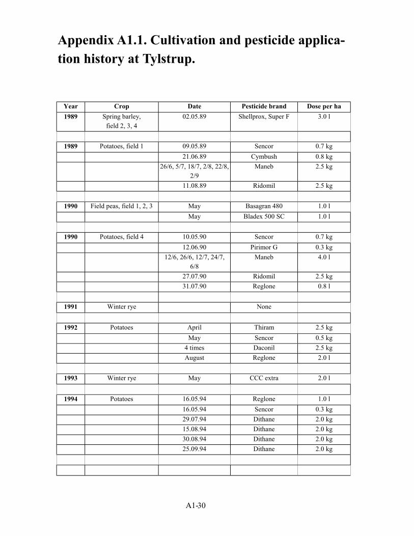
A1-30

Appendix A1.1. Cultivation and pesticide applica-

tion history at Tylstrup.

Year Crop Date Pesticide brand Dose per ha

1989 Spring barley,

field 2, 3, 4

02.05.89 Shellprox, Super F 3.0 l

1989 Potatoes, field 1 09.05.89 Sencor 0.7 kg

21.06.89 Cymbush 0.8 kg

26/6, 5/7, 18/7, 2/8, 22/8,

2/9

Maneb 2.5 kg

11.08.89 Ridomil 2.5 kg

1990 Field peas, field 1, 2, 3 May Basagran 480 1.0 l

May Bladex 500 SC 1.0 l

1990 Potatoes, field 4 10.05.90 Sencor 0.7 kg

12.06.90 Pirimor G 0.3 kg

12/6, 26/6, 12/7, 24/7,

6/8

Maneb 4.0 l

27.07.90 Ridomil 2.5 kg

31.07.90 Reglone 0.8 l

1991 Winter rye None

1992 Potatoes April Thiram 2.5 kg

May Sencor 0.5 kg

4 times Daconil 2.5 kg

August Reglone 2.0 l

1993 Winter rye May CCC extra 2.0 l

1994 Potatoes 16.05.94 Reglone 1.0 l

16.05.94 Sencor 0.3 kg

29.07.94 Dithane 2.0 kg

15.08.94 Dithane 2.0 kg

30.08.94 Dithane 2.0 kg

25.09.94 Dithane 2.0 kg

A1-31


1995 Field peas 08.05.95 Basagran 0.8 l

08.05.95 Stomp SC 0.75 l

05.08.95 Roundup 1.5 l

1996 Winter wheat 22.05.96 Activa 1.0 l

22.05.96 Herbatox 0.6 l

10.07.96 Tilt Turbo 0.4 l

05.08.96 Roundup 1.5 l

1997 Winter rape 10.09.96 Benasalox 0.4 l

10.09.96 Agil 0.25 l

05.06.97 Agil 0.5 l

1998 Winter barley 18.09.97 Boxer 0.5 l

18.09.97 Stomp 0.4 l

18.09.97 IPU 0.25 l

13.05.98 Express 0.0075 kg

13.05.98 Starane 180 0.5 l

13.05.98 Mangan 2.0 kg

17.07.98 Roundup 2.0 l

A2-1



Annexe 2.

Site 2: Jyndevad

A2-2


A2-3


The test field is located at Store Jyndevad in southern Jutland (Figure A2.1). It is leased

by the Danish Institute of Agricultural Sciences (DIAS), which has an experimental

station 0.5 km NNE of the area. Site characteristics are summarized in Table A2.1.

Table A2.1. Site characteristics.Length and width of the test field 184 x 135 m



Municipality Tinglev

County

Land registry no.Sønderjylland

47, Burkal Sogn, Tinglev

Ownership Private, leased by DIAS

Earlier use

The area is leased from a private farmer and has previously been farmed as a normal

field. As is apparent from Figure A2.2, the field has been farmland since at least 1934.

For the past few years it has been divided into a western part and an eastern part with

different cropping histories. Cultivation and pesticide application history of the test field

during the 4 years prior to the present investigations is summarized in Appendix 2.1.


All installations at Jyndevad are numbered according to the code described in Section 3.

In the present description, however, the site-specific code for Jyndevad, i.e. “2”, has

been omitted for the sake of simplicity. The locations of all installations were selected

on the basis of the groundwater flow pattern (Figure A2.3) and are shown in Figure

A2.4.

Buffer zone

The width of the buffer zone at Jyndevad is 24 m along the northern border, 16 m along

the western border, 14 m along the southern border and 3 m along the eastern border,

where the wind break acts as an additional buffer zone (Figure A2.4).


The suction cups, TDR and Pt-100 sensors at Jyndevad were installed in excavations S1

and S2 shown in Figure A2.4. The instruments were installed as described in Section

3.3 except that installation of the suction cups deviated as follows:

A2-4


from the edge of the field rather than 2 m as described in Section 3.3.


from the edge of the field rather than 2.5 m as described in Section 3.3.

Wells

Piezometers

Piezometers P1–P7 consist of ¾" electroplated pipes hammered into the ground. The

remaining piezometers were drilled with a 6" (152 mm) solid stem auger down to

around 4 m b.g.s. At deeper levels, below the groundwater table, the wells were drilled

as cased wells using a bailer.

Figure A2.2. Topographic map 1:20.000 from 1934. The test field is marked as a red

square.

A2-5

"Lille Jyndevad"

K(west)

DGU 727

P1

P2 P3

P4

DGU 509(east)

River Station

Trekant (east)

P9P10

P8P11

P5

P7P6

0 200 m

N

12.00

12.50

13.00

13.50

14.00

Figure A2.3. Potential head (m a.s.l.) at the site measured in September 1999, and the

direction of the groundwater flow.

A2-6

0 50 m

N

#

#

#

##

%

%

%

%$Z$Z$Z

P8

P11

P10

S2

S1

P9

#

#

M7

M6M5

M4

M3

M2

M1


% Piezometer

# Monitoring well

Shed

$Z Rain Gauge

Buffer Zone


A2-7

Piezometers P1–P7 were installed at the end of January 1999 in order to estimate the

flow direction of the groundwater. In the area framed by piezometers P1–P4 (Figure

A2.3), groundwater flow was highly influenced by the river immediately north of the

area. An area further away from the river was thus selected instead (Figure A2.3). Pie-

zometers P8–P11 were drilled on April 26–19 1999. The piezometers are placed at vari-

ous depths in accordance with Table A2.2.

Table A2.2. Depth of the piezometer screens.Well no. DGU no. Upper

screen

m b.g.s.

Middle

screen

m b.g.s.

Lower

screen

m b.g.s.

P1 – 6.5–6.6 – –

P2 – 5.8–5.9 – –

P3 – 6.7–6.8 – –

P4 – 6.1–6.2 – –

P5 – 5.2–5.3

P6 – 4.7–4.8

P7 – 4.7–4.8

P8 167–1346 3.4–3.9 7.6–8.1 11.0–11.5

P9 167–1345 4.0–4.5 7.6–8.1 11.2–11.7

P10 167–1347 3.4–3.9 7.4–7.9 11.4–11.9

P11 167–1348 3.4–3.9 7.4–7.9 10.9–11.4

Vertical monitoring wells


wells were installed at Jyndevad in May 31–June 6 1999 (Figure A2.4). The top of the

upper screen from each monitoring cluster was placed above the highest seasonal water

table. The screens of one monitoring cluster were not necessarily placed at the same

depths as the screens of other monitoring clusters (Table A2.3) due to minor variations

in the topography within the buffer zone resulting in differences in the distances be-

tween the ground surface and the groundwater table.

Table A2.3. Depth of the monitoring well screens.Monitoring well

cluster

Screen Mx.1

m b.g.s.

Screen Mx.2

m b.g.s.

Screen Mx.3

m b.g.s.

Screen Mx.4

m b.g.s.

M1 0.6–1.6 1.6–2.6 2.6–3.6 3.6–4.6

M2 1.0–2.0 1.9–2.9 2.9–3.9 4.0–5.0

M3 0.9–1.9 2.1–3.1 3.2–4.2 4.1–5.1

M4 1.4–2.4 2.4–3.4 3.3–4.3 4.4–5.4

M5 1.6–2.6 2.7–3.7 3.7–4.7 4.7–5.7

M6 1.4–2.4 2.4–3.4 3.4–4.4 4.5–5.5

M7 1.6–2.6 2.6–3.6 3.6–4.6 4.6–5.6

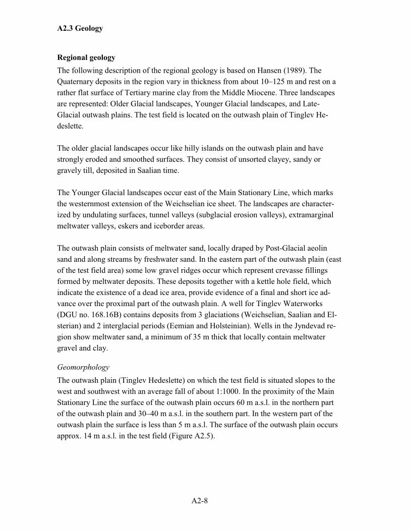
A2-8

A2.3 Geology

Regional geology

The following description of the regional geology is based on Hansen (1989). The

Quaternary deposits in the region vary in thickness from about 10–125 m and rest on a

rather flat surface of Tertiary marine clay from the Middle Miocene. Three landscapes

are represented: Older Glacial landscapes, Younger Glacial landscapes, and Late-

Glacial outwash plains. The test field is located on the outwash plain of Tinglev He-

deslette.

The older glacial landscapes occur like hilly islands on the outwash plain and have

strongly eroded and smoothed surfaces. They consist of unsorted clayey, sandy or

gravely till, deposited in Saalian time.

The Younger Glacial landscapes occur east of the Main Stationary Line, which marks

the westernmost extension of the Weichselian ice sheet. The landscapes are character-

ized by undulating surfaces, tunnel valleys (subglacial erosion valleys), extramarginal

meltwater valleys, eskers and iceborder areas.

The outwash plain consists of meltwater sand, locally draped by Post-Glacial aeolin

sand and along streams by freshwater sand. In the eastern part of the outwash plain (east

of the test field area) some low gravel ridges occur which represent crevasse fillings

formed by meltwater deposits. These deposits together with a kettle hole field, which

indicate the existence of a dead ice area, provide evidence of a final and short ice ad-

vance over the proximal part of the outwash plain. A well for Tinglev Waterworks

(DGU no. 168.16B) contains deposits from 3 glaciations (Weichselian, Saalian and El-

sterian) and 2 interglacial periods (Eemian and Holsteinian). Wells in the Jyndevad re-

gion show meltwater sand, a minimum of 35 m thick that locally contain meltwater

gravel and clay.

Geomorphology

The outwash plain (Tinglev Hedeslette) on which the test field is situated slopes to the

west and southwest with an average fall of about 1:1000. In the proximity of the Main

Stationary Line the surface of the outwash plain occurs 60 m a.s.l. in the northern part

of the outwash plain and 30–40 m a.s.l. in the southern part. In the western part of the

outwash plain the surface is less than 5 m a.s.l. The surface of the outwash plain occurs

approx. 14 m a.s.l. in the test field (Figure A2.5).

A2-9

0 50 m

#

#

#

#

# #r

rr

rr

rr

rr

r

r

r

r

r

r

r

r

r

r

r

r

r

$T

$T

$T

# M7

M6M5

M4

M3

M2

M1

P1 (3092)

P2(3091)

15.00

15.0

0

15.0

0

14.50

N

# Monitoring well

r Soil core sample

$T Pedological profile


P3


A2-10

Figure A2.6 shows the test field superimposed on the map of Quaternary sediments in

Denmark (Hermansen and Jacobsen,1998), the Soil Classification map and a 1999 aerial

orthophotograph of the field. As is apparent from the figure, the field is located on a soil

Figure A2.6. Location of the test field (red square) superimposed on: A) The soil typemap. JB 1: Coarse sandy soil B) Map of Quaternary sediments in Denmark, TS: LateGlacial freshwater sand. C) An aerial orthophotograph (Kampsax Geoplan, DDO1999).

A2-11

type consisting of coarse sandy soil (JB1). The map of the Quaternary deposits of Den-

mark places the field in an area of Late-Glacial freshwater sand (TS) forming part of an

outwash plain. Based on the orthophotograph, the field appears homogenous.


The geological layers were described down to 12 m and about 5 m b.g.s., respectively,

during the drilling of piezometers P8–P11 and monitoring wells M1–M7. The location

of the wells is shown in Figure A2.4.

The wells drilled at Jyndevad show that the sediments are dominated by fine to coarse-

grained sand, which in places contain gravel. Thin beds of clay and silt, generally 2–30

cm thick, occur locally (wells P9–10, M1, M3–4 and M6– M7 in Figure A2.7). The

beds are thickest and most abundant in well M3 where a silt layer approx. 45 cm thick

and two clay layers 20–30 cm thick occur within 1.15–3.2 m b.g.s. Fragments of char-

coal occur in wells P8, P11 and M7. It is difficult to see sedimentary structures in the

drilled sediments but horizontally bedding can be recognized locally.

Below the black topsoil layer the colour generally changes with increasing depth from

dark yellowish brown followed by yellow brown and brownish yellow. In the deepest

part the sediments have a light yellowish brown or light brownish grey colour. This

shows that oxic conditions occur at least down to 12 m b.g.s. Piezometer P10 differs in

that the sediments have a light olive grey colour from 10–12 m b.g.s. indicating suboxic

conditions at this depth interval.

Geology of the test pits and ditch

Sediments and especially the pedology were studied in three excavations, approx. 1.7 m

deep (P1,..P3, Figure A2.5). The following description focuses on the lithology and

primary sedimentary structures as a basis for interpreting the depositional environment.

The pedology is described in detail in Section A2.4. Generally soil formation has de-

stroyed primary sedimentary structures in the uppermost 0.5 m of the excavations.

The sediments in the excavations consist of alternating beds of fine, medium and

coarse-grained sand limited by erosional surfaces. The coarse-grained sand beds com-

monly contain gravel. The sand beds are structureless or trough cross-bedded with sets

up to 30 cm thick. In excavation P1(3092) a clay layer, approx. 5 cm thick drapes an

erosional depression approx. 2 m b.g.s.

A2-12

Figure A2.7. Cross sections based on wells at the site. The location of the wells isshown in Figure A2.4.

A2-13

Interpretation of the depositional environment

Based on knowledge of the regional geology, the sediments within the test field are in-

terpreted as having been deposited in a fluvial environment in front of a glacier. The

sand, which occasionally contains gravel, was deposited during high-energy conditions

and represents channel fill and bar deposits. In contrast, the clay and silt layers reflect

deposition during low-energy conditions, probably attributable to channel switching or

periods with low fluvial discharge.

Laboratory analyses

Grain size analysis

Grain size analysis has been carried out on six samples from the deeper levels of the site

(see Table A2.4). The grain size analysis shows that the sand consists of fine and me-

dium-grained sand or medium and coarse-grained sand. Two samples taken from clay

layers show a clay content of approx. 32% and 39%, respectively.

Table A2.4. Texture analysis of selected well sediment samples expressed as percent-age by weight.

Grain size in mm

Depth and

location

m b.g.s.

<0.002 0.002–

0.020

0.02–

0.63

<0.063 0.63–

0.125

0.125–

0.200

0.20–

0.5

0.5–

2.0

Sediment

P9(3.0) 6.8 44.3 44.8 Medium and coarse

-grained sand

P9(5.5) 2.7 11.8 36.8 42.9 5.6 Fine and medium-

grained sand

P9(8.7) 3.2 10.5 42.5 39.7 3.8 Fine and medium

grained sand

P9(12.0) 0.3 1.4 4.4 46.8 47.2 Medium and coarse-

grained sand

P10(2.9) 38.5 37.9 6.5 82.9 6.9 5.0 4.9 0.3 Clay

M4(8.7) 32.2 25.4 16.1 73.7 24.4 0.5 2.1 0.2 Clay


A2-14

Table A2.5. CaCO3 and total organic carbon (TOC) content in selected well sedi-

ment samples.

Locality Depth

m b.g.s.

TOC

%

CaCO3

%

Sediment

P8 4.7 0.17 Fine and medium-grained sand

P8 5.2 0.17 Coarse-grained sand

P8 5.7 0.08 Coarse-grained sand

P9 0.7 0 Medium-grained sand

P9 2.2 0.20 0.3 Sandy clay

P9 3.0 0.15 Medium-grained sand

P9 4.5 0.05 0 Medium-grained sand

P9 5.5 0.04 0.1 Fine and medium-grained sand

P9 5.7 0.19 2.4 Medium-grained sand

P9 6.1 0.05 1.6 Fine-medium grained sand

P9 6.5 0 Fine-medium grained sand


P9 8.0 0.2 Fine-medium grained sand

P9 8.7 0.04 0.7 Fine-medium grained sand

P9 9.8 0 Fine-medium grained sand


P9 12.0 0.06 4.2 Medium-grained sand

P10 2.9 0.14 1.2 Clay

M4 2.1 0.14 0 Clay



The TOC and CaCO3 data are shown in Figure A2.8 and Table A2.5. In sediments con-

taining carbonate, the carbonate content fluctuates with depth with maximum values of

4.2%. The total organic carbon content is about 1.4% in the topsoil layer at the test pits.

Below the topsoil layer it decreases with increasing depth from about 0.18% to 0.04%

in the deepest parts.

A2-15

TOC (wt-%)Grain size distribution (%) CaCO3 (wt-%)

mb.g.s.

Lithology LEGEND

Meltwater clay

SoilMeltwater sand

Chemical transition


0% 20% 40% 60% 80% 100% 0 1 2 3 4 05 0,5 1 1,5�y�y�y�y�y�y�y�y�y�y�y�y�y

0

1

2

3

4

5

6

7

8

9

10

11

12

Clay

Silt F M CSand

P9 Lithology

< 63 µm63–125 µm

200–500 µm0.5–2 mm

125–200 µm

Figure A2.8. Lithology of well P9, grain size distribution and CaCO3 and total organiccarbon (TOC) content in the test pit. Grain size fractions larger than 2.0 mm are notincluded in the grain size analysis.

A2-16

A2.4 Pedology

The pedological fieldwork at Jyndevad was carried out from May 25 to May 27 1999.

Three soil profiles were excavated and described (Figure A2.5). One of these is located

beside one of the groups of suction cups and only described in the field. In the buffer

zone, 22 soil cores were collected to a depth of 120 cm (Figure A2.5). Inside the field,

48 soil samples were collected from the topsoil (0–25 cm).

Profile description

The pedological descriptions of the three profiles are summarized in Tables A2.6 to

A2.8. The profile horizons are shown in Figure A2.9. Laboratory data (grain size, tex-

ture, organic matter, nutrients, and major cations) on the profiles are given in Table

A2.9 and Table A2.10.






(3092 West)

The profile had a diagnostic B horizon

and will be classified as a Podsol. With

no further characteristics it is a

Typipodsol.

In view of the fact that the base saturation is

>50%, the epipedon is mollic. Despite the

spodical characteristics, the Bhs horizon

does not meet the colour, Fe and Al re-

quirements of spodical material and the

horizon is therefore Cambic. In view of the

mollic epipedon, the order is Inceptisol. In

view of the udic soil moisture regime, it is

an Udept. In view of the high base satura-

tion of up to 75 cm, the soil is an Eutrudept.

Because of the distribution of sandy parti-

cles the soil is therefore an Arenic

Eutrudept.

2

(3091 South)

do. In view of the mollic epipedon, the order is

Inceptisol. In view of the udic soil moisture

regime, it is a Udept. With a base saturation

<60% from 25 to 75 cm this profile is a

Dystrudept. Moreover, because it has a

mollic epipedon and a sandy texture it is a

Humic Psammentic Dystrudept.

A2-17

Table A2.6. Description of profile 1 (3092 St. Jyndevad West).Soil classification, DK Typipodsol Soil classification, USDA Arenic Eutrudept

Parent material Glaciofluvial sand Profile depth 150 cm

UTM 32 U NF

Easting 507716

Northing 6083324


Landform Glaciofluvial plain Groundwater level 175 cm

Map sheet 1211 IV NV Vegetation Spring barley




Profile description

Ap (0–31 cm)

Black (10YR 2/1 f) clayey sand, containing humus, a few small stones of varying shape and

type, frequent fine roots, 1–10 pores per dm2, abrupt smooth boundary.

Bhs (31–42 cm)

Black (7.5YR 2.5/2 f) sand, containing humus, a few small stones of varying shape and type,

a few fine roots, very little mottled thin coatings of clay minerals and humus between the

grains of sand, weak thin granular structure, clear irregular boundary.

Bs (42–73 cm)

Dark yellowish brown (10YR 4/6 f) sand with intermixture of coarse sand, humus poor, a few

small stones of varying shape and type, very little mottled thin coatings of clay minerals

between the grains of sand, gradual wavy boundary.

BC (73–120 cm)

Yellowish brown (10YR 5/6 f) clayey sand with bands of silty sand, a few rounded medium

clear primary spots with diffuse boundary (7.5 5/6 f), secondary spots (10YR 5/4 f), humus

poor, no stones, gradual wavy boundary.

C (120–150 cm)

Light yellowish brown (10YR 6/4 f) sand, with spots (10YR 8/1 f), humus poor, no stones.

Remarks The Ap horizon contains pale quartz sand corn.

The BC and C horizons have cross-bedding structures of approx. 10 cm thick sand layers with

silty brown stripes/layers (10YR 4/2 f).

A2-18

Table A2.7. Description of profile 2 (3091 St. Jyndevad South)Soil classification, DK Typipodsol Soil classification, USDA Humic Psammentic

Dystrudept


UTM 32 U NF

Easting 507810

Northing 6083075



Map sheet 1317 III SV Vegetation Spring barley

Elevation 15 DNN Maximum rooting 50 cm



Profile description

Ap (0–33 cm)


type, artificial liming, frequent fine roots, 1–10 wormholes and root channels per dm2, very

weak granular structure, smooth abrupt boundary.

Bhs (33–45 cm)

Black (5YR 2.5/1 f) clayey sand, containing humus, a few small stones of varying shape and

type, some fine roots, weak coarse subangular structure, continuous thin coating of clay min-

erals and humus between grains of sand, clear irregular boundary.

Bs (45–89 cm)

Dark yellowish brown (10YR 3/6 f) clayey sand, humus poor, a few small stones of varying

shape and type, very weak structure, diffuse wavy boundary.

BC (89–110 cm)

Yellowish brown (10YR 5/4 f) clayey sand with intermixture of coarse sand, humus poor, a

few small stones of varying shape and type, very weak structure, diffuse wavy boundary.

C (110–150 cm)

Brownish yellow (10YR 6/6 f) sand, humus poor, a few small stones of varying shape and

type, many horizontal stripes of thin conspicuous spots with diffuse boundary.

Remarks C horizon: Red iron bands that follow the fine laminated structures.

A2-19

Table A2.8. Description of profile 3 (St. Jyndevad North).Soil classification, DK Typipodsol Soil classification, USDA Humic Psammentic

Dystrudept


UTM 32 U NF

Easting 507741

Northing 6083272



Map sheet 1317 III SV Vegetation Spring barley

Elevation 15 DNN Maximum rooting 50 cm



Profile description

Ap (0–30 cm)


type, artificial liming, frequent fine roots, 1–10 wormholes and root channels per dm2, very

weak granular structure, smooth abrupt boundary.

Bhs (30–48 cm)

Black (5YR 2.5/1 f) clayey sand, containing humus, a few small stones of varying shape and

type, some fine roots, weak coarse subangular structure, continuous thin coatings of clay

minerals and humus between grains of sand, clear broken boundary.

Bs (48–73 cm)


shape and type, very weak structure, no roots, gradual wavy boundary.

BC (73–84 cm)


shape and type, very weak structure, diffuse wavy boundary.

C (84–160 cm)

Light yellowish brown (10YR 6/4 f), humus poor, a few small stones of varying shape and

type, lots of horizontal strips of medium conspicuous spots with diffuse boundary.

Textural band: Yellowish brown (10YR 5/6 f) medium silty sand, with a few horizontally

striped diffuse mottles of dark yellowish brown (10YR 4/4 f).

Remarks None.

A2-20

Ap

Bhs

Bs

Profile 2 (3091St. Jyndevad)

BC

C

0 100 200 cm

50

100

150cm

Ap

Bhs

Bs

BC

C

Profile 1 (3092 St. Jyndevad)

0 100 200 cm

50

100

150cm

Figure A2.9. Schematic drawings of the profiles showing horizon distribution. Rectan-gular boxes indicate sampling points for soil texture and soil chemistry. Triangularboxes indicate sampling points for hydrological analysis.

A2-21


no.

Hor.

no.


%

OM1

%

cm <0.002 0.002–

0.02

0.02–

0.63

0.63–

0.125

0.125–

0.2

0.2–

0.5

0.5–2

1 1 Ap 17–27 5.3 3.2 1.0 5.0 9.9 55.1 18.3 – 2.3

1 2 Bhs 33–42 4.6 1.8 1.0 2.8 6.8 61.2 20.6 – 1.3

1 3 Bs 51–61 4.0 1.4 1.0 1.4 5.4 63.3 23.2 – 0.3

1 4 BC 85–95 5.9 0.5 1.0 4.5 46.1 41.2 0.7 – 0.1

1 5 BC 97–105 9.6 0.9 1.0 4.4 36.8 46.2 0.9 – 0.3

1 6 C 137–147 3.0 0.5 1.0 2.1 8.4 78.4 6.5 – 0.1

2 1 Ap 13–23 5.2 2.8 1.6 9.7 19.2 46.4 11.7 – 3.4

2 2 Bhs 34–44 5.6 1.9 1.3 6.6 14.9 50.3 17.5 – 1.9

2 3 Bs 67–77 4.0 0.5 1.0 3.4 11.7 54.5 24.4 – 0.5

2 4 BC 97–107 3.5 0.9 1.0 2.6 5.8 46.2 39.7 – 0.3

2 5 C 124–134 3.4 0.5 1.0 1.1 7.1 78.6 8.2 – 0.1

1) OM: Organic matter. Om = 1.72 x TOC. Analysed by DIAS.


no.

Hor.

no.


bases

H+ CEC Base

Sat.

Fe

(Ox)

Al


1 1 0.11 12 545 6.17 0.28 0.06 5.27 0.42 6.03 0.57 6.6 91 1612 944

1 2 0.06 13 268 5.82 0.05 0.04 2.71 0.27 3.07 0.43 3.5 88 1252 1952

1 3 0.03 6 142 5.77 0.04 0.02 0.76 0.14 0.96 0.74 1.7 57 828 1414

1 4 0.02 3 106 5.68 0.13 0.02 1.77 0.4 2.32 0.78 3.1 75 992 1010

1 5 0.03 6 87 4.45 0.17 0.03 2.47 0.3 2.97 2.53 5.5 54 1220 1264

1 6 0.02 3 79 4.41 0.03 0.01 0.15 0.02 0.21 0.99 1.2 18 796 636

2 1 0.13 15 440 5.64 0.19 0.07 6.12 0.5 6.88 1.72 8.6 80 1428 874

2 2 0.06 18 209 5.55 0.04 0.03 3.32 0.18 3.57 2.63 6.2 58 2016 2200

2 3 0.03 10 144 4.99 0.03 0.01 0.39 0.02 0.45 1.45 1.9 24 936 1848

2 4 0.03 6 100 5.92 0.03 0.02 0.57 0.03 0.65 0.95 1.6 41 1088 1680

2 5 0.02 3 84 5.39 0.02 0.01 0.27 0.02 0.32 0.88 1.2 27 1252 1032



The samples from the topsoil inside the field were analysed for total organic carbon

(TOC), which varied between 1.4 and 2.2% (dry weight), with a mean of 1.8±0.2%. The

concentration is highest in the southwestern part of the field and lowest in the northeast-

ern part of the field (see Figure A2.10).

A2-22


The soil cores show that with few exceptions, the succession of horizons is the same in

the entire area. The thickness of the Ap horizon varies from 23 to 33 cm. The thickness

of the Bhs horizon varies from 7 to 25 cm in the entire area. Below this lies the Bs hori-

zon with a diffuse lower border.

N

0 50 m

#

#

M7

M6M5

M4

M3

M2

M1

$T

$T

$T

1.5

1.75

2.02.25

0.50.751.01.251.51.752.02.252.52.753.04.05.08.0

.

TOC (%)


A2-23


Hansen (1976), Heidmann (1989) and Greve et al.(1998) have previously carried out

pedological and soil type investigations at the experimental station. These profiles all lie

northeast of the test field at a distance of 0.4–1.4 km. Data are also available for a

Square Grid Profile (Statens Planteavlsforsøg, 1996) approx. 2.5 km to the southwest.

The grain size distribution of the plough layer in profile 1 (West) is 55% coarse medium

sand, approx. 20% coarse sand, and 5.3% clay. A texture band at a depth of 100 to 130

cm contains 9.6% clay. In the C horizon the texture is better sorted containing 78%

coarse medium sand. To some extent the distribution is the same in profile 2 (South),

although the texture band is missing. The six reference profiles (mentioned above) all

show very similar grain size distribution, i.e. approx. 60–70% coarse medium sand and

coarse sand. Due to the coarse grain size distribution the soil is almost structureless ex-

cept in the Bhs horizon, which has a slightly coarse subangular structure due to humus,

Fe, and Al deposition.

Only the Bhs and the Bs horizons remain from what was most likely the original suc-

cession of horizons (OA, E, Bh, Bhs and Bs) (Figure A2.9). Eluvial material (washed-

out E horizon) was only found at a single drilling site. Bleached quartz sand grains were

found in the plough layer – a trace of a previous E horizon. The raw humus layer (OA)

and the washed-out horizon (E) have been mixed by ploughing, and the carbon content

has subsequently been enhanced by fertilization.

It can also be seen that the fertilization has resulted in increased phosphorous levels in

the Ap horizon (Table A2.10). The high content of Fe and Al in the Bhs horizon to-

gether with the high C/N ratio clearly shows that the soil has been podsolized. In profile

1 (West) the Al and Fe levels are not coincidental as the Fe content is higher in the

plough layer whereas the Al content is highest in the Bhs horizon. This must be attribut-

able to the greater mobility of aluminium (Duchafour, 1979) and the fact that the Bh

horizon may have been incorporated into the plough layer. A podsol would normally

have a low pH (approx. 4) that increased with increasing depth. Because of agricultural

use of lime, however, the pH profile is now the reverse, pH being highest near the sur-

face. The soil should be characterized as a partially developed podsol since the Bhs ho-

rizon is only faintly cemented (Duchafour, 1979). The expected, strongly cemented Bh

horizon (hard pan layer) is absent, probably having been removed by cultivation.

The rooting depth is only about 40 cm and has been demonstrated in both the present

investigation and by Nielsen and Møberg (1985).

A2-24

The soil is generally well drained as far as the profiles go, although red bands of iron

deposits in profile 2 (South) bear witness of faintly hydromorph features due to tempo-

rary water storage above the underlying texture band (Table A2.7). The soil cores ex-

hibit the same, but in the more low-lying southwestern part of the area, where the

groundwater table is approx. 1 m b.g.s. Above this there is a 40 cm thick BC horizon

with reddish iron deposits and faintly striped pseudogley.

Soil hydrology




The soil water characteristics for the nine small cores (100 cm3) from each horizon are

shown together with bulk density and porosity in Table A2.12 and Figure A2.11.

Ks

Kunsat

0.10 0.20 0.30 0.40 0.50


4.0

3.0

2.0

1.0

pF

A

B

C

1 10 100

h (cm)

10-8

10-7

10-6

10-5

10-4

10-3

K(m

/s)

A

B

C


A

B

C

Horizons

Horizons

A B

Figure A2.11. A) Retention curve based on values for the soil-water potential deter-mined on the small soil cores samples (100 cm3). The data are the mean values from thethree profiles. B) The unsaturated hydraulic conductivity (Kunsat) as a function of soilwater potential in cm H2O and the saturated hydraulic conductivity (Ks) determined onthe large soil cores (6,280 cm3).

A2-25



cm2


cm3/cm3

Bulk

density

g/cm3

Porosity1

cm3/cm3

1.0 1.2 1.7 2.0 2.2 3.0 4.2

1 (3092) Ap 15 0.41 0.40 0.23 0.19 0.17 0.12 0.04 1.37 0.48

Bhs/Bs 40 0.35 0.33 0.15 0.11 0.10 0.07 0.01 1.49 0.44

BC 115 0.34 0.32 0.10 0.06 0.06 0.04 0.01 1.52 0.43

2 (3091) Ap 15 0.40 0.39 0.28 0.22 0.20 0.13 0.05 1.42 0.47

Bhs/Bs 40 0.39 0.36 0.20 0.15 0.14 0.10 0.03 1.38 0.48

C 130 0.34 0.28 0.09 0.07 0.06 0.05 0.01 1.48 0.44

3( North) Ap 15 0.39 0.38 0.22 0.17 0.16 0.11 0.03 1.43 0.46

Bhs 40 0.37 0.35 0.10 0.07 0.07 0.05 0.03 1.47 0.44

C 110 0.34 0.32 0.09 0.06 0.05 0.04 0.01 1.50 0.43

1) Assuming a particle density of 2.65 g/cm3.

2) Mid-point of soil core

The soil water characteristics show that due to a low water-holding capacity most of the

water drains out of the soil at a pF value of 2. The majority of the soil pores are about

100 ←m (tube-equivalent diameter), see Figure A2.12.


(6,280 cm3) are shown in Figure A2.11. Hydraulic conductivity was high ranging from

saturation until a soilwater potential of about –30 cm H2O, whereafter the conductivity

decreased rapidly. The lowest values are found in the Ap horizon because of the higher

organic matter content than in the B and C horizons. Compared to the more loamy soils,

inter-measurement variability is low.

Measurements of saturated hydraulic conductivity and air permeability using small (100

cm3) or large (6,280 cm3) soil samples did not reveal any significant differences due to

the weakly structured nature of the soil. The soil sample is thus representative irrespec-

tive of whether a small or a large soil sample is used for the analysis.

A2-26

4

3

2

1

4

3

2

1

4

3

2

1

3000

300

3030.3

0.0

3

5 4 3 2 1 0

3000

300

3030.3

0.0

3

5 4 3 2 1 0

3000

300

3030.3

0.0

3

5 4 3 2 1 0 pF

D

A B C


n= 10n= 11

n= 10

n= 14

n= 15n= 13

n=27

n=27

n=27

n=27

n=27 n=27

A_l A_s B_l B_s C_l C_s A_l A_s B_l B_s C_l C_s

Air permeability

10-1 0

10-11

10-1 2

10-1 3

K(m

)a,

50

2

l s l s l s

A B C

Saturated hydralic conductivity

10-8

10-7

10-6

10-5

10-4

10-3

K(m

/s)

s

l s l s l s

A B C

k


A2-27



use EM-38 and ground-penetrating radar.

EM-38

The EM-38 recordings revealed only minor variation (Figure A2.14). A 20 m wide band

of higher values crosses the area from the west to east. The same pattern is seen in small

areas scattered throughout the test field. The band and the small areas can also be seen

as dark shadows on the orthophotograph. This is attributable to minor depressions in the

topography with a higher content of humus-rich horizons or thicker humus-rich

#

#

M7

M6M5

M4

M3

M2

M1

N

0 50 m

� m203040506080100160320640

mS/s

33.350.025.020.016.712.510.06.33.11.6

320

320

320

Figure A2.14. Resistivity maps of the area.

A2-28

horizons. Compared with the TOC (A2.10), there is no obvious connection to the car-

bon content of the plough layer, however.


The ground-penetrating radar mapping was conducted using 100 MHz aerials and a pre-

sumed wave velocity of 0.130 m/ns along a grid lines at 20 m x 20 m. The reflectors on

the GPR cross sections generally form complex structures indicating cross-bedding and

horizontal beds of varying grain size. The penetration depth varies from 7–16 m. Areas

where the penetration depth is greater than 12 m seem to be randomly distributed. In

areas where the penetration depth is low this may be due to the occurrence of one or

more silt/clay layers near the ground surface or because the mean grain size of the

sediments is lower than in the remaining areas. Several of the clay horizons occurring in

the wells are seen as continuous reflectors, up to 100 m long, in the georadar cross sec-

tions. The clay layer occurring 2.9–3.2 m b.g.s. at monitoring well M3 probably corre-

sponds to the thin clay layer occurring 2.8 m b.g.s. at monitoring well M1, as indicated

on the N-S georadar cross section 1 (Figure A2.15). The clay layer has not been ob-

served in monitoring well M2, however, as would have been expected on the basis of

the GPR cross section. The thin clay layer occurring 3.6 m b.g.s. at monitoring well M7

can be followed on the S-N georadar cross section 3 over a distance of approx. 100 m

starting immediately north of piezometer P11. The same clay layer is seen as an approx.

60 m long reflector on the E-W georadar cross section 12. This indicates that some of

the clay layers observed in the wells cover relatively large areas within the test field.


A2-29

Appendix A2.1. Cultivation and pesticide applica-

tion history at Jyndevad.


Western part

1995 Spring barley Express §

Dantril §


Dantril §

Roundup §

1997 Potatoes Sencor WG 0.35 kg

Unknown fungicides §

1998 Potatoes Sencor WG 0.35 kg

Unknown fungicides §

1999 Spring barley 10.05.1999 Logran 20 WG 0.015 kg

10.05.1999 Mantrac (manganese

fertilizer)

Eastern part


Dantril §

1996 Peas Unknown §

1997 Winter wheat Biotril 0.5 l

1998 Maize Roundup 2.0 l

Gardoprim 1.5 l

Lentagran 2.0 l

1999 Spring barley 10.05.1999 Logran 20 WG 0.015 kg

10.05.1999 Mantrac (manganese)

§) Information of the dose does not exist.

A3-1



Annexe 3.

Site 3: Silstrup

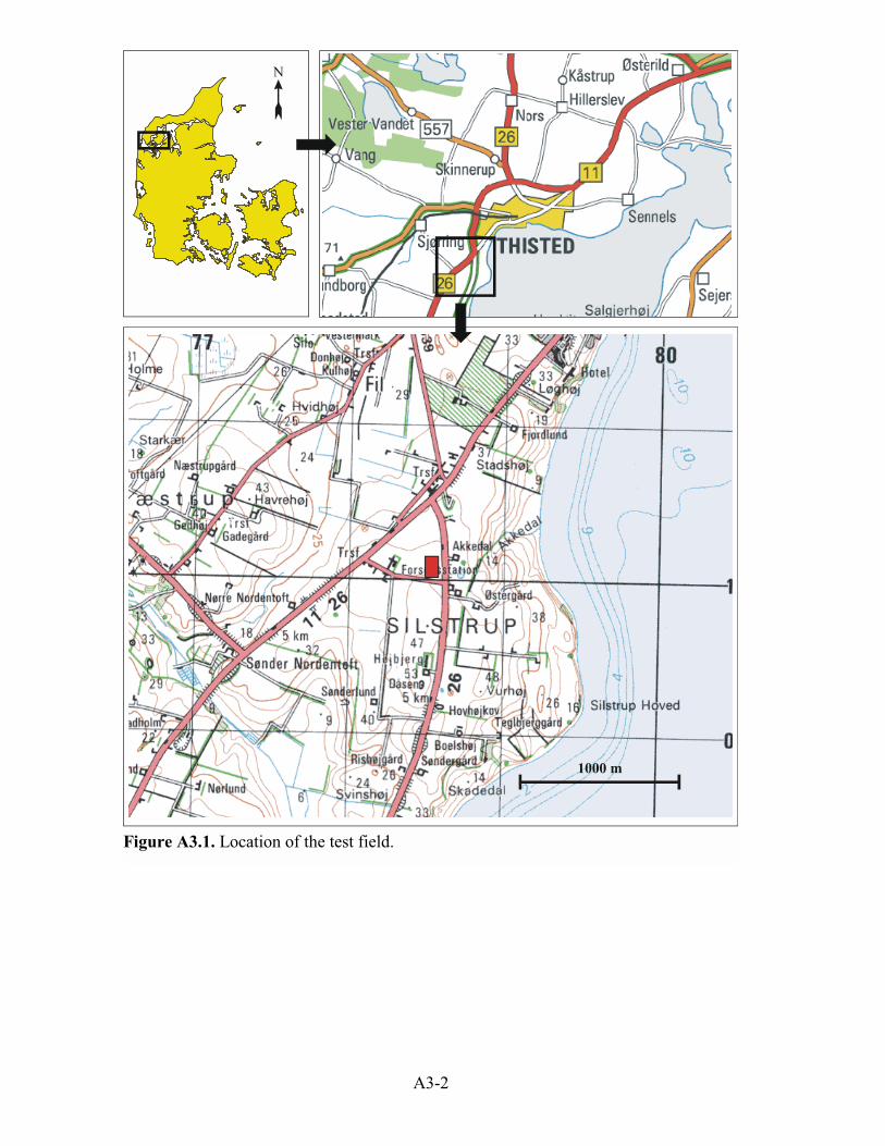
A3-2


A3-3


The test field is situated at Silstrup south of Thisted in northwestern Jutland (Figure

A3.1), and is owned by the Danish Institute of Agricultural Sciences (DIAS). The site

characteristics are summarized in Table A3.1.

Table A3.1. Site characteristics.

Length and width of the test field 185 m x 91 m



Municipality Thisted

County

Land registry no.

Viborg

2a, Silstrup, Tilsted

Ownership DIAS, Silstrup Experimental Station

Højmarken 12

7700 Thisted

Earlier use

As is apparent from Figure A3.2, the field has been farmland at least since 1942. In

1966 the area was systematically drained, as seen in Figure A3.4. The area had been

farmed as a normal field for the preceding 17 years, and had not been used for plot ex-

periments. Cultivation and pesticide application history of the field during the 17 years

prior to the present investigations are summarized in Appendix A.3.1.

After work on the site installations had been initiated it was discovered that the road just

east of the site had previously traversed part of the test field (Figure A3.2). The road was

apparently straightened in the 1940s. As the presence of an old roadbed or associated

earthworks might influence the hydraulic properties of the area, the test field was moved

45 m further to the west.


All installations at Silstrup are numbered according to the code described in Section 3.

In the present description, however, the site-specific code for Silstrup, i.e. “3”, has been

omitted for the sake of simplicity. The locations of all installations were selected on the

basis of the drainage system and the groundwater flow pattern (Figure A3.3) and are

shown in Figure A3.4.

A3-4

Buffer zone

The width of the buffer zone is 18 m along the western and eastern borders, and 5 m

along the southern border, where a small road acts as an additional buffer zone. North of

the field the buffer zone is more than 10 m wide.

Suction cups, TDR and Pt-100 sensors.

The suction cups, TDR and Pt-100 sensors at Silstrup were installed in two excavations

S1 and S2 (Figure A3.4) in accordance with Section 3.3.

Figure A3.2. Topographic map 1:20.000 from 1942. The test field is marked as a redsquare. New road system is shown in black.

A3-5

Wells

Horizontal sampling wells

Two 58 m, long horizontal sampling wells H1 and H2 were installed (Figure A3.4),

each of which consists of three 18 m screen sections separated by 1 m bentonite seals.

The first screens in both wells (H1.1 and H2.1) are located within a lateral distance of

17 m from the western edge of the test field.

#

##

#

#

#

#

#

#

0 50 m

M11

M13

M9

M5 M6

M10

M12M3

N%

%

%

%

%

%

%

%

%

#

#

P4

M4

M7P1

M1

M8

M2

P3

P2

%

%

%

%

%

%

%

%

%

36.00

36.50

Figure A3.3. Potential head (m a.s.l.) at the site measured in February 2000 and the

direction of the ground water flow.

A3-6

0 50 m10 m

N

$Z$Z %

%

%

%

%

%

%

%

%

#

##

#

#

#

#

P4

M4S1

S2

M7P1

M1

M8

H1

H2

P3

0 50 m

#

#

M11

M13

M9

M5 M6

M10

M12M3

P2

M2

Outlet


% Piezometer

# Monitoring well

Shed

$Z Rain Gauge



Collector pipe


Buffer Zone

Horizontal screen


A3-7

The wells were drilled perpendicular to the edge of the field. The screens are 3.5 m

b.g.s. The depth of well H1 deviates up to 0.09 m from the intended position of 3.5 m

b.g.s., whereas well H2 deviated 0.34 m. According to the drilling company, part of H2

follows a “pavement”, probably a clay till rich in stones and boulders.

Installation of piezometers

All wells at Silstrup were drilled as cased wells with a 6" (152 mm) solid stem auger. In

some sandy intervals below the groundwater head, however, a bailer was used to clean

the borehole before installation of the screen.

As a preliminary survey, one borehole was drilled in February 1999 (DGU no. 30.1120)

near to well P3 in the southeastern corner of the field. Rafts of glacially dislocated Ter-

tiary clay were found in this borehole and it was therefore decided to abandon it and

look for a better location.

In May 1999, however, it was decided to go ahead with the site, and three wells P1, P2

and P4 each containing three piezometers were drilled in order to start monitoring the

groundwater head. In august 1999 a third well, P3, containing three piezometers was

drilled. The depth of the piezometers at Silstrup is summarized in Table A3.2.

Table A3.2. Depth of the piezometer screens.Well

no.

DGU no. Upper

screen

m b.g.s.

Middle

screen

m b.g.s.

Lower

screen

m b.g.s.

P1 30. 1123 2.0-2.5 3.5-4.0 11.5-12.0

P2 30. 1122 3.0-3.5 5.5-6.0 11.5-12.0

P3 30. 1191 3.0-3.5 6.1-6.6 11.2-12.2

P4 30. 1124 2.75-3.25 4.5-5.0 11.5-12.0

Monitoring wells

A total of 13 monitoring well clusters (M1–M13) each consisting of four individual

wells were installed at Silstrup from August 8 1999 to September 9 1999. The technical

specifications are described in Section 3.1.2.

A3-8

The monitoring well screens of all 13 clusters are located at the following depths:

Mx.1: 1.5–2.5 m b.g.s.

Mx.2: 2.5–3.5 m b.g.s.

Mx.3: 3.5–4.5 m b.g.s.

Mx.4: 4.5–5.5 m b.g.s.

Monitoring well clusters M1 to M8 were installed first. Thereafter it was decided to

relocate the area 45 meters to the west, as described above. Monitoring well clusters M9

to M13 were thereafter installed to cover the new area. The new area also encompasses

well clusters M4 and M8. This was considered acceptable provided that the two well

clusters were not used for monitoring.

Drainage system

The experimental station was systematically drained by DIAS in the 1960s. To facilitate

experimental work, the drainage system for each field is separate. The drains were laid

manually in open machine-excavated trenches. The design of the drainage system is

illustrated in Figure A3.4.

The design of the drainage system in the test field is simple, consisting of five parallel

field drains running from south to the north end, where they connect to a transverse

collector drain. In the northeast corner of the field the collector drain is connected to a

main drain, which runs northwards alongside the major public road.

The drainpipes are clayware, with an inner diameter of 6.5 cm for laterals and 8 cm and

10 cm for the mains. The lateral drains are enveloped by seashells (mussel shells) to

improve permeability.

The initial plan was to place the measuring chamber at the northeastern corner and to

establish relatively simple and short pipe connections to the existing drainage system.

Due to relocation of the site, however, this had to be changed.

New collector pipes and measuring chamber

The two easternmost pipes were severed and replaced by two similar drains from the

neighbouring field to the west. The measuring chamber was placed in the northeastern

corner of the revised field boundary. As the two new drains had their outflow towards

the west, a new pipe had to be installed to lead the water from the northwestern corner

to the measuring chamber in the northeastern corner. This was done with 90 metres of Ø

90 mm PE pipe along the northern boundary of the experimental field. The slope of the

A3-9

pipe is only 2‰. The collector pipe carrying the water from the three other drainpipes

was connected close to the chamber by a few meters of Ø 110 mm PE pipe (outer di-

ameter) with plenty of slope. These pipes are watertight, welded in situ.

The measuring chamber is made from Ø 125 cm concrete rings and has a 30° v-notch

weir. To collect the water from the two new drains to the west, the chamber had to be

placed 75 cm deeper than the original drainpipe and with limited slope in the outlet.

Dimension of the outlet

The main 10 cm drainpipe along the public road has a rather steep slope of 13–16‰. To

obtain slope from the chamber, the outlet was established 60 m downstream. The pipe

used is a Ø 160 mm smooth PVC pipe with rubber fittings. The PVC pipe was con-

nected to the existing 10 cm clay pipe by a PVC T-junction. The slope of the new pipe is

only 2‰, but giving an elevation of 5–10 cm near the chamber.

The drained area of the experimental field is 1.69 ha. The capacity of the new 160 mm

pipe is approx. 10 l sec-1 ha-1, which should be ample. If there are limitations, these

should be found further downstream in the 10 cm tile drain, which has a water-carrying

capacity of approx. 6 l sec-1 ha-1 and a catchment area of 3 ha.

On several occasions during the season 1999/2000, however, the water level in the

measuring chamber rose above the notch by more than a 1 m.

New information on the upstream catchment area revealed that two fields south of the

experimental field were connected to the main pipe such that the catchment area is actu-

ally almost three times the expected area. This connection was not shown on the original

map of the drainage system, and probably explains the inadequate capacity of the old

main. Additional information was compiled on the conditions downstream. It revealed

that new pipes had been installed on the neighbouring field and under the road, probably

in 1994 in connection with regulation of the main road. Approx. 200 m north of the

measuring chamber there is a new main drain with a much higher capacity.

In September 2000 the outlet from the measuring chamber was disconnected from the

old 10 cm main and extended 160 m to the north. The new pipe is a Ø 160/140 mm cor-

rugated pipe without perforations. The lower end was connected to an inspection cham-

ber from where the drain continues as a 160/145 mm corrugated drainpipe installed

around 1994. The new stretch has an average slope of 16‰. The outlet from the meas-

uring chamber runs eastwards perpendicular to the road for the first 36 m and thereafter

182 m northward parallel to the road a few meters west of the old main drain. The first

A3-10

60 m consist of watertight smooth PVC pipes tightened with rubber rings, while the rest

is watertight corrugated PE pipe in 25 m lengths, assembled with non-tight connections.

The initial work was carried out in August 1999 and the main work in September 1999,

while the outlet was extended in September 2000.

A3.3 Geology

Regional geology

The area around Silstrup displays a number of spectacular geological features. The most

prominent – a salt dome called the Thisted Structure – considerably influences the local

geology. Vertical movement of 3 to 4 km within the dome has brought Tertiary and

Cretaceous chalk to the surface just north of Silstrup. The salt in the dome is still rising,

the uplift in the area being estimated at 2.5 mm/yr (Hansen and Håkansson, 1980). A

number of terminal moraines formed by the Great Belt–North Jutland re-advance during

the Late Weichselian (Houmark-Nielsen, 1987), and which can be traced from the city

of Randers to Thy, comprise another important regional geological element. Around

Silstrup these terminal moraines often consist of glaciotectonic thrust fault complexes

where Tertiary sediments such as the Paleocene-Eocene diatomite and Oligocene mica

clay and glacial sediments such as clay till and glaciofluvial clastics are important ele-

ments in the thrust sheets (Gry, 1940; Klint and Pedersen, 1995). Just east of the test

field in the coastal cliff Silstrup Hoved there is a thrust sheet complex in a coastal cliff

section consisting of Paleocene diatomite and Oligocene mica clay. The test field is lo-

cated on a ridge complex overlain by a till cover.

According to Gry (1940), the fold axis orientation at Silstrup Hoved is 166° caused by

deformation from the east. The same direction can be observed in the long axis of the

elongated hills in the area around Silstrup, probably reflecting the same deformation

phase. The presence of other fold axis orientations (personal communication: Stig

Schack Pedersen, GEUS) proves that there have been several deformation phases in the

area. On the basis of the varied fold axis orientation patterns in the coastal cliffs around

Thisted Bredning, Gry (1940) interpreted the present day depression (Thisted Bredning)

as the product of a glacial lobe formed during the Late Weichselian. The variety of fold

axis orientations in the area could also be attributable to a number of ice advances of

different ages leaving different orientations as a consequence of a series of glaciotec-

tonic events.

A3-11

r

r

r

r

r

r

r

rrrr

r

r

r

r

r

r

r

r

r

r

#

##

#

#

#

#

#

$T

$T

#

#

0 50 m

M11

M13

M9

M5 M6

M10

M12M3

P2(3094)

P1(3093)

38.00

40.00

39.00

37.00

N

$T

# Monitoring well

r Soil core sample

Pedological profile


Test pit


A3-12

Geomorphology

The test site is situated between 36 and 45 m a.s.l. close to the top of an elongated hill.

The surface slopes approx. 2.2% towards NNE (see Figure A3.5). 200 m east of the site

the surface drops abruptly from 30 m a.s.l. to sea level.

Figure A3.6 shows the field superimposed on the map of Quaternary sediments in Den-

mark (Hermansen and Jacobsen, 1998), the Soil Classification map and a 1999 aerial

orthophotograph of the field. As is apparent, the field is located on a loamy soil (JB7).

This is in good agreement with the fact that the map of the Quaternary sediments of

Denmark places the field in an area of ML, which is a clay till. Based on the orthopho-

tograph, the field appears to be homogenous.

Geology of the monitoring wells and piezometer wells.

The wells drilled at Silstrup revealed a homogenous cover of clay till rich in chalk and

chert of Cretaceous and Early Tertiary origin. Cross sections containing the wells drilled

at the site are found in Figure A3.7 and A3.8. According to grain size analysis (Table

A3.4 and Figure A3.11) the clay till consists of clay (20–35%), silt (20–40%) and sand

(20–40%). Gravel constitutes approx. 5%, but occasionally up to 20%. The CaCO3

content ranges from 20 to 45% by weight in the clay till. At some intervals the till has

been described as a sandy till (MS), i.e. contains less than 12–14% clay.

Thin layers and lenses of glaciofluvial sand (DS) are found in some wells, often de-

scribed as alternating thin beds of sand occasionally with silt and clay stringers (VS).

None of these layers can be correlated.

In M3, M12 and P3, Oligocene clay and silt were encountered, presumably “Cilleborg

Clay” (Gry, 1940; personal communication: Peter Roll Jakobsen, GEUS). In M12, Oli-

gocene clay was encountered at 2.5 m b.g.s. – the most shallow occurrence at the site. In

all wells where Oligocene sediments were penetrated, clay till was found underneath. As

a consequence, all Oligocene sediments in the test field are glacially dislocated. In sev-

eral wells in the region, glaciotectonites with Oligocene clays and silt were found

(Pedersen, 1989).

Three levels of oxidation can be observed in the upper 12 m of the till. In most wells an

upper zone with yellowish brown and brownish yellow coloration is found from below

the topsoil to a depth varying from 2.5 to 5 m b.g.s. Below this a suboxic zone with

greyish brown till is found to a depth of 4 to 6 m b.g.s. This zone is typically 0.2 to 0.5

m thick. Below this zone there is a reduced zone of olive grey and grey-coloured till.

A3-13

Figure A3.6. Location of the test field (red square) superimposed on: A) The soil typemap. JB 5/6: Sandy loam soil, JB 7: Loamy soil. B) Map of Quaternary sediments inDenmark, ML: Clay till. C) An aerial orthophotograph (Kampsax Geoplan, DDO1999).

A3-14

M6

M3

M9M10

P4 M4

M8

M12

5.60

5.60

5.605.60

12.00

5.60

5.60

5.60

��@@@@��ÀÀÀÀ��@@@@��ÀÀÀÀ��@@@@��ÀÀÀÀ��yyyy

��

@@@@@@

��

ÀÀÀÀÀÀ

��

@@@@@@

��

ÀÀÀÀÀÀ

��

@@@@@@

��

ÀÀÀÀÀÀ

��

yyyyyy

��

@@@@@@

��

ÀÀÀÀÀÀ

��

@@@@@@

��

ÀÀÀÀÀÀ

��

@@@@@@

��

ÀÀÀÀÀÀ

��

yyyyyy

��

@@@@@@

��

ÀÀÀÀÀÀ

��

@@@@@@

��

ÀÀÀÀÀÀ

��

@@@@@@

��

ÀÀÀÀÀÀ

��

yyyyyy

��

@@@@@@

��

ÀÀÀÀÀÀ

��

@@@@@@

��

ÀÀÀÀÀÀ

��

@@@@@@

��

ÀÀÀÀÀÀ

��

yyyyyy

��

@@@@@@@@

��

ÀÀÀÀÀÀÀÀ

��

@@@@@@@@

��

ÀÀÀÀÀÀÀÀ

��

@@@@@@@@

��

ÀÀÀÀÀÀÀÀ

��

yyyyyyyy

��

@@@@@@@@

��

ÀÀÀÀÀÀÀÀ

��

@@@@@@@@

��

ÀÀÀÀÀÀÀÀ

��

@@@@@@@@

��

ÀÀÀÀÀÀÀÀ

��

yyyyyyyy

��

@@@@@@@@

��

ÀÀÀÀÀÀÀÀ

��

@@@@@@@@

��

ÀÀÀÀÀÀÀÀ

��

@@@@@@@@

��

ÀÀÀÀÀÀÀÀ

��

yyyyyyyy

��

@@@@@@@@

��

ÀÀÀÀÀÀÀÀ

��

@@@@@@@@

��

ÀÀÀÀÀÀÀÀ

��

@@@@@@@@

��

ÀÀÀÀÀÀÀÀ

��

yyyyyyyy

��

@@@@@@@@

��

ÀÀÀÀÀÀÀÀ

��

@@@@@@@@

��

ÀÀÀÀÀÀÀÀ

��

@@@@@@@@

��

ÀÀÀÀÀÀÀÀ

��

yyyyyyyy

��

@@@@@@@@

��

ÀÀÀÀÀÀÀÀ

��

@@@@@@@@

��

ÀÀÀÀÀÀÀÀ

��

@@@@@@@@

��

ÀÀÀÀÀÀÀÀ

��

yyyyyyyy

��

@@@@@@@@

��

ÀÀÀÀÀÀÀÀ

��

@@@@@@@@

��

ÀÀÀÀÀÀÀÀ

��

@@@@@@@@

��

ÀÀÀÀÀÀÀÀ

��

yyyyyyyy

��

@@@@@@@@

��

ÀÀÀÀÀÀÀÀ

��

@@@@@@@@

��

ÀÀÀÀÀÀÀÀ

��

@@@@@@@@

��

ÀÀÀÀÀÀÀÀ

��

yyyyyyyy

��

@@@@@@

��

ÀÀÀÀÀÀ

��

@@@@@@

��

ÀÀÀÀÀÀ

��

@@@@@@

��

ÀÀÀÀÀÀ

��

yyyyyy

��

@@@@@@

��

ÀÀÀÀÀÀ

��

@@@@@@

��

ÀÀÀÀÀÀ

��

@@@@@@

��

ÀÀÀÀÀÀ

��

yyyyyy

��

@@@@@@

��

ÀÀÀÀÀÀ

��

@@@@@@

��

ÀÀÀÀÀÀ

��

@@@@@@

��

ÀÀÀÀÀÀ

��

yyyyyy

��

@@@@@@

��

ÀÀÀÀÀÀ

��

@@@@@@

��

ÀÀÀÀÀÀ

��

@@@@@@

��

ÀÀÀÀÀÀ

��

yyyyyy



��

@@@@@@

��

ÀÀÀÀÀÀ

��

@@@@@@

��

ÀÀÀÀÀÀ

��

@@@@@@

��

ÀÀÀÀÀÀ

��

yyyyyy

��

@@@@@@

��

ÀÀÀÀÀÀ

��

@@@@@@

��

ÀÀÀÀÀÀ

��

@@@@@@

��

ÀÀÀÀÀÀ

��

yyyyyy

��

@@@@@@

��

ÀÀÀÀÀÀ

��

@@@@@@

��

ÀÀÀÀÀÀ

��

@@@@@@

��

ÀÀÀÀÀÀ

��

yyyyyy

��

@@@@@@

��

ÀÀÀÀÀÀ

��

@@@@@@

��

ÀÀÀÀÀÀ

��

@@@@@@

��

ÀÀÀÀÀÀ

��

yyyyyy

��

@@@@@@

��

ÀÀÀÀÀÀ

��

@@@@@@

��

ÀÀÀÀÀÀ

��

@@@@@@

��

ÀÀÀÀÀÀ

��

yyyyyy

��

@@@@@@

��

ÀÀÀÀÀÀ

��

@@@@@@

��

ÀÀÀÀÀÀ

��

@@@@@@

��

ÀÀÀÀÀÀ

��

yyyyyy

��

@@@@@@

��

ÀÀÀÀÀÀ

��

@@@@@@

��

ÀÀÀÀÀÀ

��

@@@@@@

��

ÀÀÀÀÀÀ

��

yyyyyy

��

@@@@@@

��

ÀÀÀÀÀÀ

��

@@@@@@

��

ÀÀÀÀÀÀ

��

@@@@@@

��

ÀÀÀÀÀÀ

��

yyyyyy

��

@@@@@@

��

ÀÀÀÀÀÀ

��

@@@@@@

��

ÀÀÀÀÀÀ

��

@@@@@@

��

ÀÀÀÀÀÀ

��

yyyyyy

��

@@@@@@

��

ÀÀÀÀÀÀ

��

@@@@@@

��

ÀÀÀÀÀÀ

��

@@@@@@

��

ÀÀÀÀÀÀ

��

yyyyyy

��

@@@@@@

��

ÀÀÀÀÀÀ

��

@@@@@@

��

ÀÀÀÀÀÀ

��

@@@@@@

��

ÀÀÀÀÀÀ

��

yyyyyy

��

@@@@@@

��

ÀÀÀÀÀÀ

��

@@@@@@

��

ÀÀÀÀÀÀ

��

@@@@@@

��

ÀÀÀÀÀÀ

��

yyyyyy

Soil

Clay till

Sand till

Glaciofluvial sand

Glaciofluvial clay

Oligocene clay and silt

Screen

Horizontal scale 1:2000Vertical scale 1:200

��

@@@@@@

��

ÀÀÀÀÀÀ

��

@@@@@@

��

ÀÀÀÀÀÀ

��

@@@@@@

��

ÀÀÀÀÀÀ

��

yyyyyy

44

42

40

38

36

34

32

30

m a.s.l. m a.s.l.

N S

44

42

40

38

36

34

32

30

44

42

40

38

36

34

32

30

m a.s.l. m a.s.l.

N S

44

42

40

38

36

34

32

30

Figure A3.7. N-S cross sections based on wells at the site. The location of the wells isshown in Figure A3.4.

A3-15

46

44

42

40

38

36

34

32

12.40

5.60

5.60

12.30

m a.s.l.

E W

E W

P2

M3

M12 P3

12.10 12.00

5.605.605.50

32

34

36

38

40

42

32

34

36

38

40

42P1

M7 M6 M5P4

Soil

Clay till

Sand till

Glaciofluvial sand

Glaciofluvial clay

Oligocene clay and silt

Screen


46

44

42

40

38

36

34

32

m a.s.l. m a.s.l.

m a.s.l.

��

@@@@@@@@

��

ÀÀÀÀÀÀÀÀ

��

@@@@@@@@

��

ÀÀÀÀÀÀÀÀ

��

@@@@@@@@

��

ÀÀÀÀÀÀÀÀ

��

yyyyyyyy

��

@@@@@@@@

��

ÀÀÀÀÀÀÀÀ

��

@@@@@@@@

��

ÀÀÀÀÀÀÀÀ

��

@@@@@@@@

��

ÀÀÀÀÀÀÀÀ

��

yyyyyyyy

��

@@@@@@@@

��

ÀÀÀÀÀÀÀÀ

��

@@@@@@@@

��

ÀÀÀÀÀÀÀÀ

��

@@@@@@@@

��

ÀÀÀÀÀÀÀÀ

��

yyyyyyyy

��

@@@@@@

��

ÀÀÀÀÀÀ

��

@@@@@@

��

ÀÀÀÀÀÀ

��

@@@@@@

��

ÀÀÀÀÀÀ

��

yyyyyy

��

@@@@@@

��

ÀÀÀÀÀÀ

��

@@@@@@

��

ÀÀÀÀÀÀ

��

@@@@@@

��

ÀÀÀÀÀÀ

��

yyyyyy

��

@@@@@@

��

ÀÀÀÀÀÀ

��

@@@@@@

��

ÀÀÀÀÀÀ

��

@@@@@@

��

ÀÀÀÀÀÀ

��

yyyyyy

��

@@@@@@

��

ÀÀÀÀÀÀ

��

@@@@@@

��

ÀÀÀÀÀÀ

��

@@@@@@

��

ÀÀÀÀÀÀ

��

yyyyyy

��

@@@@@@

��

ÀÀÀÀÀÀ

��

@@@@@@

��

ÀÀÀÀÀÀ

��

@@@@@@

��

ÀÀÀÀÀÀ

��

yyyyyy

��

@@@@@@

��

ÀÀÀÀÀÀ

��

@@@@@@

��

ÀÀÀÀÀÀ

��

@@@@@@

��

ÀÀÀÀÀÀ

��

yyyyyy

��

@@@@@@

��

ÀÀÀÀÀÀ

��

@@@@@@

��

ÀÀÀÀÀÀ

��

@@@@@@

��

ÀÀÀÀÀÀ

��

yyyyyy

��

@@@@@@

��

ÀÀÀÀÀÀ

��

@@@@@@

��

ÀÀÀÀÀÀ

��

@@@@@@

��

ÀÀÀÀÀÀ

��

yyyyyy��

@@@@@@

��

ÀÀÀÀÀÀ

��

@@@@@@

��

ÀÀÀÀÀÀ

��

@@@@@@

��

ÀÀÀÀÀÀ

��

yyyyyy

��

@@@@@@

��

ÀÀÀÀÀÀ

��

@@@@@@

��

ÀÀÀÀÀÀ

��

@@@@@@

��

ÀÀÀÀÀÀ

��

yyyyyy

��

@@@@@@

��

ÀÀÀÀÀÀ

��

@@@@@@

��

ÀÀÀÀÀÀ

��

@@@@@@

��

ÀÀÀÀÀÀ

��

yyyyyy

��

@@@@@@

��

ÀÀÀÀÀÀ

��

@@@@@@

��

ÀÀÀÀÀÀ

��

@@@@@@

��

ÀÀÀÀÀÀ

��

yyyyyy

��

@@@@@@

��

ÀÀÀÀÀÀ

��

@@@@@@

��

ÀÀÀÀÀÀ

��

@@@@@@

��

ÀÀÀÀÀÀ

��

yyyyyy

��

@@@@@@@@

��

ÀÀÀÀÀÀÀÀ

��

@@@@@@@@

��

ÀÀÀÀÀÀÀÀ

��

@@@@@@@@

��

ÀÀÀÀÀÀÀÀ

��

yyyyyyyy

��

@@@@@@

��

ÀÀÀÀÀÀ

��

@@@@@@

��

ÀÀÀÀÀÀ

��

@@@@@@

��

ÀÀÀÀÀÀ

��

yyyyyy

��

@@@@@@@@

��

ÀÀÀÀÀÀÀÀ

��

@@@@@@@@

��

ÀÀÀÀÀÀÀÀ

��

@@@@@@@@

��

ÀÀÀÀÀÀÀÀ

��

yyyyyyyy

��

@@@@@@

��

ÀÀÀÀÀÀ

��

@@@@@@

��

ÀÀÀÀÀÀ

��

@@@@@@

��

ÀÀÀÀÀÀ

��

yyyyyy

��

@@@@@@@@

��

ÀÀÀÀÀÀÀÀ

��

@@@@@@@@

��

ÀÀÀÀÀÀÀÀ

��

@@@@@@@@

��

ÀÀÀÀÀÀÀÀ

��

yyyyyyyy

��

@@@@@@

��

ÀÀÀÀÀÀ

��

@@@@@@

��

ÀÀÀÀÀÀ

��

@@@@@@

��

ÀÀÀÀÀÀ

��

yyyyyy

��

@@@@@@

��

ÀÀÀÀÀÀ

��

@@@@@@

��

ÀÀÀÀÀÀ

��

@@@@@@

��

ÀÀÀÀÀÀ

��

yyyyyy

��

@@@@@@

��

ÀÀÀÀÀÀ

��

@@@@@@

��

ÀÀÀÀÀÀ

��

@@@@@@

��

ÀÀÀÀÀÀ

��

yyyyyy

��

@@@@@@

��

ÀÀÀÀÀÀ

��

@@@@@@

��

ÀÀÀÀÀÀ

��

@@@@@@

��

ÀÀÀÀÀÀ

��

yyyyyy

��

@@@@@@

��

ÀÀÀÀÀÀ

��

@@@@@@

��

ÀÀÀÀÀÀ

��

@@@@@@

��

ÀÀÀÀÀÀ

��

yyyyyy

��

@@@@@@

��

ÀÀÀÀÀÀ

��

@@@@@@

��

ÀÀÀÀÀÀ

��

@@@@@@

��

ÀÀÀÀÀÀ

��

yyyyyy

��

@@@@@@

��

ÀÀÀÀÀÀ

��

@@@@@@

��

ÀÀÀÀÀÀ

��

@@@@@@

��

ÀÀÀÀÀÀ

��

yyyyyy

��

@@@@@@

��

ÀÀÀÀÀÀ

��

@@@@@@

��

ÀÀÀÀÀÀ

��

@@@@@@

��

ÀÀÀÀÀÀ

��

yyyyyy


��

@@@@@@

��

ÀÀÀÀÀÀ

��

@@@@@@

��

ÀÀÀÀÀÀ

��

@@@@@@

��

ÀÀÀÀÀÀ

��

yyyyyy

��

@@@@@@@@

��

ÀÀÀÀÀÀÀÀ

��

@@@@@@@@

��

ÀÀÀÀÀÀÀÀ

��

@@@@@@@@

��

ÀÀÀÀÀÀÀÀ

��

yyyyyyyy

��

@@@@@@

��

ÀÀÀÀÀÀ

��

@@@@@@

��

ÀÀÀÀÀÀ

��

@@@@@@

��

ÀÀÀÀÀÀ

��

yyyyyy

Figure A3.8. E-W cross sections based on wells along the southern and northern ends ofthe test field. The location of the wells is shown in Figure A3.4.

A3-16

Geology of the test pit and drainage ditch excavations

A test pit was excavated to 5.0 m b.g.s. using a backhoe in the buffer zone of the north-

eastern corner of the test field (Figure A3.5) for field vane tests, fracture descriptions

and characterization, fabric analysis, and lithological description. Samples were taken

for grain size analysis, CaCO3 content, clay mineral analysis, and exotic stone counts.

Lithological description

The depths in the following descriptions (Table A3.3) are average depths from the test

pit, and correspond to the log in Figures A3.9–A3.11. The description follows Larsen et

al,(1995).

Table A3.3. Lithological descriptions from the test pit at Silstrup.

Depth

m b.g.s.

Description Sample

number0.0–0.5 Topsoil, dark brown to black, numerous biopores and desiccation fractures. DIAS

0.5–1.0 Clay till, strong mix of sand and gravel, yellowish brown, noncalcareous. DIAS

1.0–1.3 Clay till, mix of silt, sand strong mix of gravel, some pebbles and boulders,

yellowish brown with pale olive spots. Calcareous in some parts of the profile

from 1.0 m b.g.s. Heavily fractured.

DIAS

1.3–1.5 Clay till, weak mix of silt and sand, mix of gravel clay veins, strong brown.

Thickness varies from 40 to 25 cm. At 1.3 m b.g.s. a small fold axis in a folded

sand vein was measured to 42/8 indicating a deformation from southeast.

8803

1.5–3.5 Clay till, mix of silt, weak mix of sand, strong mix of gravel, lots of chert and

chalk fragments in the gravel fraction, fractures with Fe and Mn oxides. Light

yellowish brown. Calcareous. A number of fractures were encountered in the

suboxic zone, which were olive coloured (5Y 4/3).

8804 +

8805 +

8806

3.5–5.0 Clay till, mix of silt, weak mix of sand, strong mix of gravel and pebbles, olive

grey, rich in chert and chalk. Very few fractures with Fe oxides reach 4.0 m

b.g.s. Calcareous.

At 4.25 m b.g.s. striation was measured on a rock to 02/18 indicating a defor-

mation from the north.

8807 +

8808 +

8840 +

8841

Fracture description

In order to develop a conceptual model of the fracture systems and macropores at the

test field, fracture system parameters were measured in the test pit excavation: orienta-

tion at various depths, positions and frequencies. On the basis of these measurements, a

number of fracture parameters were calculated. In Figure A3.9 and A3.10, the data are

plotted and the fracture systems described according to Klint and Gravesen (1999). Be-

A3-17

sides the fracture analysis, fabric in the till and fold axis in folded sand veins were

measured in order to describe the stratigraphic relations in the test pit excavation.

Fracture trace frequency was measured in two profiles in the test pit excavation, a north-

facing wall and an east-facing wall. In general the fracture systems at Silstrup are domi-

nated by postdepositional fractures attributable to desiccation and cryogenic processes.

From the surface and to 0.7–0.8 m b.g.s. in the test pit excavation, desiccation fractures

and biopores dominate to such a degree as to preclude proper estimation of the fracture

trace frequency. This unit can be described as heavily fractured and bioturbated. At 0.6

m b.g.s. there were an estimated 400 biopores/m2.

From 0.7 to 1.8 m b.g.s. the till is intensely fractured by a horizontal/subhorizontal

fracture system, possibly connected to freeze-thaw processes in a periglacial environ-

ment, or to horizontal shear from a glacier.

0.7 m b.g.s.

1.3 m b.g.s.

2.0 m b.g.s.

4.0 m b.g.s.

3.5 m b.g.s.

2.0 m b.g.s.

NN=25

N=27

N=24

N

N

N

N

NN=27

N=15

N=35

N

N=35

2.0 m b.g.s.

N

N=15

3.5 m b.g.s.

Clast fabricOrientations of vertical fractures

Structures

Lit

holo

gy

Fracture systems Orientation

mb.g.s.

Ice movement

Lithology

LithologyTectonic structures

Biogene structures

LEGEND

Sandy Till

Soil

��Sand

Clay Till

Stones��Clay/Silt

RootsBurrows

Fractures

0

0.5

1

1.5

2

2.5

3

3.5

4

4.5

5

. . . .

Chemical transition

NoncalcareousCalcareousOxidated matrixReduced matrix

Figure A3.9. Lithology, fracture orientation, clast fabric data and interpreted ice move-ment direction.

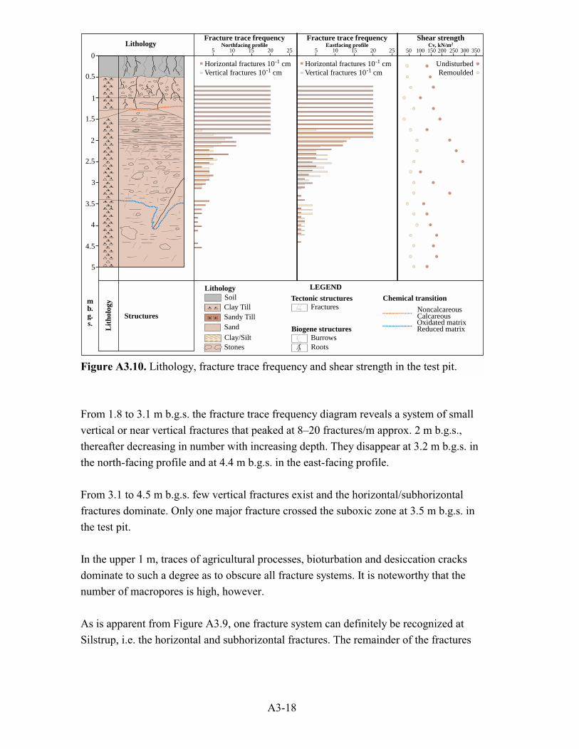
A3-18

From 1.8 to 3.1 m b.g.s. the fracture trace frequency diagram reveals a system of small

vertical or near vertical fractures that peaked at 8–20 fractures/m approx. 2 m b.g.s.,

thereafter decreasing in number with increasing depth. They disappear at 3.2 m b.g.s. in

the north-facing profile and at 4.4 m b.g.s. in the east-facing profile.

From 3.1 to 4.5 m b.g.s. few vertical fractures exist and the horizontal/subhorizontal

fractures dominate. Only one major fracture crossed the suboxic zone at 3.5 m b.g.s. in

the test pit.

In the upper 1 m, traces of agricultural processes, bioturbation and desiccation cracks

dominate to such a degree as to obscure all fracture systems. It is noteworthy that the

number of macropores is high, however.

As is apparent from Figure A3.9, one fracture system can definitely be recognized at

Silstrup, i.e. the horizontal and subhorizontal fractures. The remainder of the fractures

Structures

Lit

holo

gymb.g.s.

Lithology


Biogene structures

LEGEND

Sandy Till

Soil

�Sand

Clay Till

Stones�Clay/Silt

RootsBurrows

Fractures

0

0.5

1

1.5

2

2.5

3

3.5

4

4.5

5

. . . .

Chemical transition


5 10 15 20 25 5 10 15 20 25 50 100 150 200 250 300 350

UndisturbedRemoulded

Horizontal fractures 10-1 cmVertical fractures 10-1 cm


Fracture trace frequencyNorthfacing profile

Fracture trace frequencyEastfacing profile

Shear strengthCv, kN/m2

Figure A3.10. Lithology, fracture trace frequency and shear strength in the test pit.

A3-19

found in the test pit represent a variety of orientations and the data set is too small to

determine whether a second or third fracture system is present.

Fracture geochemistry

Five depth-dependent types of coating could be observed on the fracture surfaces in the

test pit.

I. 0.3–1.0 m b.g.s. In the upper part of the clay till the fractures and biopores are

either coated with clay skin or topsoil. Root traces are found in many fractures.

The matrix is oxidized.

II. 1.0–2.0 m b.g.s. The fractures and biopores are surrounded by a grey halo, re-

flecting oxygen depletion and reduced conditions in the close vicinity of the

fractures caused by decomposition of organic matter. The matrix is oxidized.

III. 2.0–3.3 m b.g.s. The fractures are coated with Fe oxides and some manganese

oxides. The matrix is oxidized.

20 40 60 80 100

ClaySiltSand

TOC (wt-%)Grain size distribution (%) CaCO3 (wt-%)50 25 35 50454030201510

Structures

Lit

holo

gymb.g.s.

Lithology


Biogene structures

LEGEND

Sandy Till

Soil

��Sand

Clay Till


RootsBurrows

Fractures

0

0.5

1

1.5

2

2.5

3

3.5

4

4.5

5

. . . .

Chemical transition


0.5 1 1.5 2

Figure A 3.11. Lithology, grain size distribution and CaCO3 and total organic carbon(TOC) content in the test pit. Grain size fractions larger than 2.0 mm are not included inthe grain size analysis.

A3-20

IV. 3.3–3.5 m b.g.s. In this narrow interval an olive-coloured coating was observed

that is considered as being indicative of a fluctuating groundwater head (personal

communication: Vibeke Ernstsen, GEUS). The matrix is suboxic.

V. 3.5–5.0 m b.g.s. In the reduced clay till no coating was observed except for one

fracture that was FeO- and MnO-coated to a depth of almost 4.5 m b.g.s. The

matrix is reduced.

Clast fabric analysis

Clast fabric analyses were performed at four depths 0.7, 1.3, 2.0 and 4.0 m b.g.s. (Figure

A3.9). The analysis at 0.7 m b.g.s. revealed a weak fabric from the northeast. At 1.3 m

b.g.s. this fabric indicates a north-northeasterly direction, whereas the analysis at 2.0 m

b.g.s. revealed a strong fabric indicating iceflow from the north, an observation that is in

good agreement with a striation measured on a boulder at the same level. The lowermost

analysis revealed a weak fabric, and is nonconclusive.

Field vane tests

Field vane tests were performed in the test pit excavation at 25 cm intervals from top to

bottom (Figure A3.10). Down to a depth of 2.5 m b.g.s. the undisturbed shear strength

(Cv) increases from approx. 50 to approx. 290 kN/m2. From 2.5 to 3.0 m b.g.s. the shear

strength varies. From 3.5 to 5.5 m b.g.s. the shear strength ranges from 120 to 175

kN/m2.

Laboratory analyses

Grain size analysis

Grain size analysis has been carried out on 15 samples from the site (Table A3.4). This

describes the clay till as rich in clay, ranging from 28% to 36% clay. One sample from

1.5 m b.g.s. contained 58% clay. The Oligocene sediments are dominated by silt (40–

80%) and clay (20–30%). As they are laminated or bedded, however, individual

horizons will have higher or lower clay:silt ratio than indicated by the grain size

analysis, which will influence the hydraulic properties.

A3-21

Table A3.4. Texture analysis of sediment from the test pit and from selected wells.Grain size in mm

Depth and

location

m b.g.s.

<0.002 0.002-

0.020

0.02-

0.63

0.63-

0.125

0.125-

0.200

0.20-0.5 0.5-

2.0

Sediment

Test pit

1.5 57.8 7.6 3.8 8.8 6.4 10.6 5.1 Clay till, oxidized




3.5 30.8 27.9 7.3 7.6 6.9 13.6 6.0 Clay till, reduced



5.0 32.0 30.8 5.7 7,2 6.3 11.8 6.0 Clay till, reduced

Wells

P3(2.5) 40.2 16.1 6.0 9.6 8.0 14.0 6.2 Clay till

P3(5.5) 18.1 53.0 26.9 1.6 0.1 0.2 0.1 Oligocene silt

P3(8.5) 30.7 51.0 10.5 6.5 0.5 0.6 0.2 Oligocene silt

P3(10.0) 30.5 36.2 6.3 7.1 5,4 9.6 5.0 Oligocene clay

M7(4.0) 27.2 24.7 6.7 8.2 7.2 18.2 7.8 Sand, medium to coarse,

mix of silt, clay

M13(4.0) 27.8 34.1 6.2 6.8 6.2 12.6 6.2 Clay till

M8(1.5) 21.1 13.6 4.7 12.3 12.3 25.7 10.2 Sand, mix of clay, lami-

nated


Clay mineral analysis

Clay mineral analysis was carried out in three samples from the test pit. All three sam-

ples showed that the clay fraction (<2 ←m) in the till at Silstrup is dominated by smec-

tite. Other minerals present are vermiculite, illite, kaolinite and quartz.

Fine gravel analysis

Fine gravel analysis has been carried out on two samples from the test pit excavation

(Figure A3.12). The sample taken from 5.0 m b.g.s. reveals a local dominance of Meso-

zoic and Cenozoic limestone and flint, originating from the Thisted Structure. The sam-

ple from 1.5 m b.g.s. has a similar composition regarding the noncalcareous clasts, but a

lower content of Mesozoic and Cenozoic limestone. This might reflect both the more

shallow depth and subsequent dissolution of carbonates and a change in iceflow direc-

tion. The lower sample reflects an iceflow in close contact with the Thisted Structure

while the upper sample indicates iceflow, possibly in a southwesterly direction.

A3-22

The difference in the composition of noncalcareous clasts points towards two till units

in the test pit excavation, or at least a change in iceflow direction.


The TOC and CaCO3 data are shown in Figure A3.11 and Table A3.5. The CaCO3

content of the clay till at Silstrup is high, ranging from 21% weight to 45% weight

(mean value of 38%), reflecting the fact that the site is located in the “shadow” of the

Thisted Structure. In the test pit the mean CaCO3 content is 42% while that of the Oli-

gocene sediments found in the northern part of the field ranges from 21% to 55%.

The total organic carbon data from the test pit reveal a significant change in TOC con-

tent at 3.5 m b.g.s., where TOC doubled from 0.16 to 0.33% reflecting the transition

zone from oxic conditions to reduced conditions. In the Oligocene silt at piezometer P3

located 5.5 m b.g.s. TOC was 2.12%. In the other two Oligocene samples, however,

TOC was less than 1%.

Figure A3.12. Fine gravel analysis from two levels in the test pit. n is the number ofgrains counted.

A3-23

Table A3.5. Sediment CaCO3 and total organic carbon (TOC) content in the test pit andselected wells.Locality Depth

m b.g.s.

TOC

%

CaCO3

%

Sediment

Test pit 1.5 0.17 16 Clay till, oxidized




Test pit 3.5 0.33 42 Clay till, reduced




P3 2.5 0.19 37 Clay till

P3 5.5 2.1 21 Oligocene silt

P3 8.5 0.73 42 Oligocene clay

P3 10.0 0.29 55 Oligocene clay

M7 4.0 0.24 27 Sand, medium to coarse, mix of silt,

clay

M13 4.0 0.17 21 Clay till

M8 1.5 0.15 20 Sand, mix of clay, laminated


Porosity and permeability

No data are available from Silstrup.

A3.4 Pedology

Pedological field work

The pedological field work at Silstrup was carried out from August 30 to September 2

1999. Two soil profiles were excavated and described (Figure A3.5). These were located

beside each of the two groups of suction cups. In the buffer zone, 21 soil cores were

collected to a depth of 120 cm (Figure A3.5). Inside the field, 36 soil samples were col-

lected from the topsoil (0–25 cm).

A3-24

Table A3.6. Description of profile 1 (3093 Silstrup East).Soil classification, DK Pseudogleytypilessive Soil classification, USDA Alfic Argiudoll

Parent material Clay till Profile depth 200 cm

UTM 32V MJ

Easting 478551

Northing 6310172

Drainage class Moderately well

drained

Landform Glacial ridge complex Groundwater level 220 cm

Map sheet 1116 I NV Vegetation Stubble


Topography Gentle slope Authors Søren Torp

Slope 1-2 Date of description 30.08.99

Profile description

Ap (0-32 cm)

Greyish brown (10YR 3/2 f) clay, containing humus, a few small and medium size stones of mixed

type, some fine roots, 1-10 wormholes and root channels per dm2, very weak thin granular struc-

ture, slight sticky when wet, clear smooth boundary.

Bv (32-80 cm)

Yellowish brown (10YR 5/4 f) sandy heavy clay, humus poor, lots of small and medium size

stones of mixed form and type, a few small soft Fe and Mn oxide and hydroxide nodules of mixed

form, some fine roots, 1-10 wormholes and root channels per dm2, moderately coarse columnar

structure, sticky consistency when wet, mottled thick coatings of clay minerals and humus in root

channels and on aggregate peds, gradual wavy boundary.

Bt(g) (80-135 cm)

Yellowish brown (10YR 5/4 f) heavy clay with some vertical stripes of clear light olive brown

(2.5Y 5/4 f) spots with diffuse boundary, secondary spots of pinkish grey (7.5YR 6/2 f), humus

poor, some small and medium size stones of mixed form and type, a few small soft Fe and Mn

oxide and hydroxide nodules of mixed form, a few fine roots, 1-10 pores per dm2, strong coarse

columnar structure, very sticky consistency when moist, continuous thick coatings of clay minerals

and humus in root channels and on aggregate peds, diffuse wavy boundary.

BC(g) (135-160 cm)

Brown (10YR 5/3 f) clay with some vertical stripes, large conspicuous yellowish brown (10YR 5/8

f) spots with clear boundary, humus poor, some small and medium size stones of mixed form and

type + lumps of chalk, a few small soft Fe oxide and hydroxide nodules of mixed form, a few fine

roots, 1-10 pores per dm2, moderately coarse columnar structure, sticky consistency when wet,

continuous thick coatings of clay minerals and humus in root channels and on aggregate peds,

diffuse wavy boundary.

Cc(g) (160-200 cm)

Very pale brown (10YR 7/3 f) clayey silty sand with lots of vertical stripes of big clear brownish

yellow (10YR 6/6 f) spots with clear boundary, humus poor, lots of small and medium size stones

of mixed form and type + lumps of lime, a few small soft Fe oxide and hydroxide nodules of

mixed form, very calcareous mainly as lumps, moderately medium strong angular structure, sticky

consistency when moist, mottled, moderately thick coatings of clay minerals on aggregate peds.

Remarks Chimney continues to a depth of 230 cm.

A3-25

Table A3.7. Description of profile 2 (3094 Silstrup North).Soil classification, DK Pseudogleytypibrunjord Soil classification, USDA Typic Hapludoll


UTM 32 V MJ

Easting 478533

Northing 6310193


drained

Landform Glacial ridge complex Groundwater level 220 cm

Map sheet 1116 I NV Vegetation Stubble


Topography Gentle slope Authors Søren Torp

Slope 1-2 Date of description 31.08.99

Profile description

Ap (0-30 cm)

Very dark greyish brown (10YR 3/2 f) clay, containing humus, a few small stones of varying

shape and type, some fine roots, 1-10 pores per dm2, moderately coarse granular structure, weak

sticky consistency, clear smooth boundary.

Bv (30-60 cm)

Yellowish brown (10YR 5/4 f) clay with lots of vertical medium clear dark greyish brown

(10YR4/2 f) spots with clear boundary, humus poor, a few small stones of varying shape and type,

frequent fine roots, 1-10 pores per dm2, strong coarse angular structure, weak sticky consistency,

moderately thick mottled coatings of clay minerals and humus in root channels and wormholes,

diffuse wavy boundary.

Bv(g) (60-95 cm)

Yellowish brown (10YR 5/3 f) clay with many vertical stripes of large clear yellowish brown

(10YR 5/6 f) spots with clear boundary, humus poor, a few small and medium size stones of

mixed form and type, a few small soft rounded Fe and Mn oxide and hydroxide nodules, frequent

fine roots, 1-10 pores per dm2, strong coarse angular structure, weak sticky consistency, moder-

ately thick spotted coatings of clay minerals and humus in root channels and wormholes, clear

wavy boundary.

Cc (95-132 cm)

Very pale brown (10YR 7/3 f) clay, humus poor, a few small and medium size stones of mixed

form and type + lumps of lime, a few small soft rounded Fe and Mn oxide and hydroxide nodules,

strongly calcareous, mainly as lumps, a few fine roots, strong coarse angular structure, weak sticky

consistency, thin spotted coatings of clay minerals and humus on aggregate peds, clear wavy

boundary.

2Cc texture bands (132-155 cm)

Yellowish brown (10YR 5/4 f) clayey silt with lots of horizontal stripes, medium yellowish brown

(10YR 5/8 f) spots with clear boundary, humus poor, a few small stones of varying shape and type,

strongly calcareous mainly as lumps, moderately coarse angular structure, sticky consistency,

gradual wavy boundary.

Cc(g) (155-190 cm)

Very pale brown (10YR 7/3 f) sandy heavy clay, with lots of rounded within clear yellowish brown

(10YR 5/8 f) spots with diffuse boundary, humus poor, a few small and medium size stones of

mixed form and type + lumps of lime, a few small soft rounded Fe oxide and hydroxide nodules,

calcareous mainly as powder, strong coarse angular structure, sticky consistency in wet condition.

Remarks The Bv horizon: Vertical wormholes 4-6 mm in cross section containing humus along the edge

and some with fine roots.

The Bv(g) horizon: Thick coherent clay skins around stones.

A3-26


no.

Hor.

no.


%

OM1

%

cm <0.002 0.002–

0.02

0.02–

0.63

0.63–

0.125

0.125–

0.2

0.2–

0.5

0.5–2

1 1 Ap 10–20 18.3 16.4 13.4 16.3 8.8 16.4 7.1 – 3.4

1 2 Bv 45–55 30.1 13.9 10.9 14.9 8.5 14.1 6.9 – 0.5

1 3 Bt(g) 115–125 43.4 18.6 2.5 10.0 8.4 12.0 4.8 – 0.3

1 4 BC(g) 150–160 24.6 13.4 11.8 10.6 8.4 18.2 12.8 – 0.2

1 5 Cc(g) 190–200 11.4 9.1 11.3 8.0 5.6 13.4 3.8 37.3 –

2 1 Ap 10–20 26.6 15.4 10.2 14.9 10.4 15.3 6.4 – 2.8

2 2 Bv 46–56 27.9 14.1 12.7 15.2 8.4 15.2 6.0 – 0.5

2 3 Bv(g) 67–77 25.9 14.1 12.8 14.6 11.0 15.0 6.2 – 0.4

2 4 Cc 106–116 17.5 10.5 10.3 9.6 7.2 11.0 5.6 28.3 –

2 5 Cc(g) 138–148 34.5 11.5 5.3 11.2 6.8 10.8 4.4 15.4 0.1



no.

Hor.

no.


bases

H+ CEC Base

sat.

Fe

(Ox)

Al


1 1 0.2 10 506 6.66 0.23 0.19 17.1 0.97 18.5 2.2 20.7 89 2892 918

1 2 0.05 6 144 6.67 0.26 0.17 14.7 1.13 16.3 3.53 19.8 82 2364 1120

1 3 0.05 3 197 7.39 0.29 0.3 19.3 1.82 21.7 – 17.6 100 2624 1208

1 4 0.03 4 363 7.38 0.24 0.22 13.2 0.92 14.6 0.24 14.8 98 1700 670

1 5 0.02 – 353 7.75 0.12 0.13 19.6 0.43 20.3 – 7.4 100 750 304

2 1 0.17 10 396 7.01 0.26 0.17 17 0.87 18.3 2.07 20.4 90 2708 954

2 2 0.05 6 136 7.24 0.26 0.17 16.6 1.02 18 1.29 19.3 93 2052 1172

2 3 0.05 5 164 7.44 0.2 0.16 16.8 0.76 17.9 – 12.1 100 1200 908

2 4 0.03 – 337 7.67 0.15 0.14 20.1 0.38 20.8 – 8.3 100 740 434

2 5 0.04 1 419 7.72 0.27 0.16 26 0.68 27.1 – 21.2 100 1326 640


Profile description

The pedological descriptions of the two profiles are summarized in Tables A3.6 and

A3.7. The profile horizons are shown in Figure A3.13 while the laboratory data (grain

size, texture, organic matter, nutrients, and major cations) are summarized in Table A3.8

and A3.9.

A3-27

+

+

+

Ap

Bv

Bt(g)

BC(g)

Cc(g)

Profil 1 (3093 Silstrup East)0 100 200 cm

50

100

150

cm

+

Profil 2 (3094 Silstrup North)

Bv

Ap

Bv(g)

Cc

Cc(g)

2Cc

0 100 200 cm

50

100

150

cm

Figure A3.13. Schematic drawings of profiles showing horizon distribution. Rectangu-lar boxes indicate sampling points for soil texture and soil chemistry. Triangular boxesindicate sampling points for hydrological analysis. White areas with + symbolise stones.

A3-28

In Table A3.10 the profiles are classified according to “A Pedological Soil Classifica-

tion System Based on Danish Soils” (Madsen and Jensen, 1985) and USDA Soil Tax-

onomy (Soil Survey Staff, 1999).



(3093 East)

The soil has a Bt horizon and is therefore

a Lessive soil. As it has no further char-

acteristics it is a Typilessive. Because

there is Pseudogley, it is a Pseu-

dogleytypilessive.

The soil has a high base saturation and a

high organic matter content. It is therefore a

Mollisol, and at the sub-order level is a

Udoll. Because there is an argillic horizon,

the soil is an Argiudoll. The colour requires

it to be classified at the sub-group level as

an Alfic Argiudoll.

2

(3094 North)

Because the soil has more than 8% clay,

30% silt and no Bt horizon, it is a Brun-

jord. At the group level a Typibrunjord.

Because of the Pseudogley, it is a Pseu-

dogleytypibrunjord.

Because there is a mollic epipedon and a

high base saturation throughout the profile,

it is a Mollisol. Having no special diagnostic

horizons, the soil is a Udoll, Hapludoll and

finally, a Typical Hapludoll.


There is little variation in soil type in the area. The most common horizon subdivision is

Ap–Bv–Bt(g) and in some places Ap2, BC, C. C horizons mainly occur in the western

part of the soil cores taken from the buffer zone. The location is apparent on Figure

A3.5. The presence of Pseudogley from a depth of approx. 70 cm (40-90 cm) in soil

cores taken from the buffer zone indicates temporary water saturation during moist peri-

ods.

Comparison of the EM 38 map (Figure A3.18A) and the soil cores indicates a uniform

topsoil but a more variable clay content in the underlying soil.


The samples from the topsoil inside the test field were analysed for total organic carbon

(TOC), which varied between 1.9% and 2.4% (dry weight) with a mean of 2.2% ± 0.1%.

The concentration was lowest in the northern part of the field (Figure A3.14).

A3-29


Pedological investigations have previously been carried out at Silstrup Experimental

Station located 300 m southwest of the test field by Hansen (1976) and in relation to the

Square Grid Profile (Statens Planteavlsforsøg, 1996) located 500 m to the south.

In both profiles at the test field the plough layer contains 18–25% clay. At a depth of 1

m the clay content is 43% in profile 1 (3093 East). The percentage of clay probably de-

N

0 50 m

2.25

2.0

1.75

T

T

#

#

M11

M13

M9

M5 M6

M10

M12M3

0.50.751.01.251.51.752.02.252.52.753.04.05.08.0

.

TOC (%)


A3-30

reases towards the south since Hansen (1976) found 15% clay in the plough layer and

over 24% clay in the underlying soil. At the Square Grid Profile the clay content is 12%

in the topsoil and up to 27% at a depth of 120 cm. This picture is supported by the

EM38 measurements (Figure A3.18A).

From a pedological point of view the change in clay content related to the parent mate-

rial as well as to the different degrees of eluviation. The presence of a Bt horizon re-

vealed by the occurrence of clay skins on peds in the profiles and in many of the soil

cores is evidence of clay migration. Although evidence of clay migration could not be

confirmed in these areas because the soil is cultivated, a high clay content is found just

beneath the plough layer. The soils in these areas contain the weathered and brunified

Bv horizons.

The base saturation of the soil is high due to the presence of chalk in the parent material

and the high biological activity, both of which keep cations in circulation. The high base

saturation can be maintained for a long time and provides the soil with a strong structure

(Madsen, 1983). The C/N relation is low due to the high degree of decomposition.

Ks

Kunsat

0.10 0.20 0.30 0.40 0.50


4.0

3.0

2.0

1.0

pF

A

B

C

1 10 100

h (cm)

10-8

10-7

10-6

10-5

10-4

10-3

K(m

/s)

A

B

C


A

C

Horizons Horizons

A B

Figure A3.15. A) Retention curve based on values for the soil-water potential deter-mined on the small soil core samples (100 cm3). The data are the mean values from bothprofiles. B) The unsaturated hydraulic conductivity (Kunsat) as a function of soilwaterpotential in cm H2O and the saturated hydraulic conductivity (Ks) determined on thelarge soil cores (6,280 cm3).

A3-31

The soil in the test field can be characterized as moderately mature with only slight elu-

viation in the NW areas to mature with more pronounced eluviation of both chalk and

clay to some depth in the southern and eastern parts.

Soil hydrology




The soil water characteristics of the nine small cores (100 cm3) from each horizon are


Table A3.11. Soil water characteristics determined on the small soil cores pF = log10(-h).

Profile

no.

Hori-

zon

Depth

cm


cm3/cm3

Bulk

density

g/cm3

Porosity1

cm3/cm3

1.0 1.2 1.7 2.0 2.2 3.0 4.2

1 (3093) Ap 15 0.39 0.38 0.36 0.35 0.34 0.28 0.13 1.42 0.46

Bv 40 0.35 0.35 0.32 0.31 0.30 0.25 0.16 1.62 0.39

BC(g) 150 0.30 0.30 0.29 0.28 0.28 0.26 0.16 1.77 0.33

2 (3094) Ap 15 0.37 0.36 0.35 0.34 0.34 0.29 0.14 1.54 0.42

Bv 40 0.36 0.36 0.35 0.34 0.33 0.29 0.15 1.59 0.40

Cc 90 0.31 0.30 0.29 0.29 0.28 0.26 0.12 1.73 0.35


The soil in the A and B horizons gradually decreases in water content as a function of

pF due to the relatively uniform pore size distribution, which is typical for a

clayey/loamy soil. The majority of the pore are about 0.6 µm (tube-equivalent diameter),

see Figure A3.16. The percentage of pores >12 µm is particularly low in the C horizon.


(6,280 cm3) is shown in Figure A3.15. Unsaturated conductivity is low in all three hori-

zons, with high inter-measurement variability in the A and C horizons. Due to the high

variability in the A horizon within both the individual profiles and the field, it is diffi-

cult to establish a unique relationship between soil water potential (h) and hydraulic

conductivity (k) in the horizon. The marked difference between near-saturated

A3-32

4

3

2

1

4

3

2

1

4

3

2

1

3000

300

3030.3

0.0

3

5 4 3 2 1 0

3000

300

3030.3

0.0

3

5 4 3 2 1 0

3000

300

3030.3

0.0

3

5 4 3 2 1 0 pF

D

A B C


Air permeability

A_l A_s B_l B_s C_l C_s


A_l A_s B_l B_s C_l C_s

10-1 0

10-11

10-1 2

10-1 3

K(m

)a,

50

2

l s l s l s

A B C

10-8

10-7

10-6

10-5

10-4

10-3

K(m

/s)

s

l s l s l s

A B C

n= 6 n= 6

n= 6

n= 10

n= 9

n= 9

n=18

n=18

n=18

n=17

n=18

n=18

k


A3-33

hydraulic conductivity and saturated hydraulic conductivity indicates a high degree of

direct piping (preferential flow) through macropores when the soil is fully saturated.

The measurements of saturated hydraulic conductivity and air permeability made using

small (100 cm3) or large (6,280 cm3) soil samples differed markedly. This difference is

probably related to the structure of the soil leading to a high dependence on sample size.

With the large soil samples, infiltration takes place through a much larger soil area than

is the case with the small soil samples and a greater number of macropores and other

soil heterogeneities are therefore included.



use EM-38, CM-031 and ground-penetrating radar (GPR). The EM 38 mapping was

carried out on August 31 1999.

EM-38 mapping.

The EM-38 map found in Figure A3.18A reveals a rather homogenous texture pattern at

Silstrup near the surface, i.e. the apparent resistivity ranges from 80 to 40 τm, with that

of the majority of the area being 50 to 60 τm. In the northern end of the test field there

are two areas with apparent resistivity in the range 40 to 50 τm indicating a higher clay

content. In the areas with elevated apparent resistivity, the soil core and well data indi-

cate the presence of clay and clay loam just below the topsoil.

CM-031 mapping

The test field has also been mapped with a CM-031 conductivity meter (Figure A3.18B,

C and D). Figure A3.18B shows the apparent resistivity with a horizontal magnetic field

penetrating 2-3 m. A homogeneous field can be identified with resistivity in the range

60 to 80 τm. According to Skov- og Naturstyrelsen (1987), resistivity is relatively high

for a clay till, possibly due to the high CaCO3 content of the till (>40% by weight).

The field is dotted with a number of smaller areas of elevated resistivity (80–100 τm),

probably due to the presence of a more sandy till or sand lenses in the till. Figure

A3.18C shows the apparent resistivity with a penetration of 5 to 6 m. These data reveal

a completely homogenous geology with a resistivity between 60 and 80 τm indicating

the

A3-34

0 50 m

N

M13

M11M5 M6

M9

M10

M3M12

$T

$T

80

60

50

6080

M13

M11M5 M6

M9

M10

M3M12

$T

$T

M13

M11M5 M6

M9

M10

M3M12

$T

$T

60

80

M13

M11M5 M6

M9

M10

M3M12

$T

$T

B) Penetration depth 2.5-3 mA) Penetration depth 1 m

C) Penetration depth 5-6 m D) 2.5-3m vs 5-6 m

� m203040506080100160320

mS/s

33.350.025.020.016.712.510.06.33.1

2.5-3/5-6

0.40.60.81.01.21.61.82.02.54

Figure A3.18. Resistivity maps of the area. Map D shows the relative difference be-tween map B and C and provides an idea about the homogeneity of the electrical prop-erties to a depth of approx. 6 m b.g.s.

A3-35

presence of a clay till. The relative difference between the vertical and the horizontal

magnetic fields is shown in Figure A3.18D. Resistivity increases slightly with increas-

ing depth, the opposite of what would be expected from the geological data. Again this

may be attributable to the relatively high content of CaCO3 in the unweathered clay till.


To detect any larger sand or gravel lenses or other geological anomalies and obtain in-

formation about internal structures such as bedding planes, etc., the area was mapped

using ground-penetrating radar in a 20 to 30 m grid. The profiles revealed almost con-

tinuous cover with low penetration, interpreted as a clay till. Penetration of up to 4 m

was obtained in a few spots, however. These data are in good agreement with the resis-

tivity data.

A3-36

Appendix A3.1. Cultivation and pesticide appli-

cation history at Silstrup.


1983 Spring barley 13.06.83 Bayleton 0.3 kg

13.06.83 Propinox 2.0 l

1984 Winter barley 20.09.83 Tribunil 4.0 kg

14.11.83 Topsin 0.8 l

27.04.84 Sportak 1.0 l

23.05.84 Tilt 0.5 L

1985 Winter wheat 20.11.84 Bayleton 0.5 kg

20.11.84 Vegoran 1.75 l

14.05.85 Cycocel 1.0 l

14.05.85 M-prop-combi 3.5 l

14.05.85 Sportak 45 ec 1.0 l

1986 Spring barley 29.05.86 Decis 0.3 l

Undersown grass 29.05.86 Dinoseb 1.5 l

29.05.86 Manganchelat 1.0 l

29.05.86 Parathion 1.0 l

1987 Grass

1988 Field bean 30.05.88 Dinoseb 1.2 l

25.10.88 Roundup 3.0 l

1988 Spring barley 01.06.88 D-prop-mix 3.0 l

28.06.88 Sportak 45 ec 0.5 l

1989 Fodder beet 27.04.89 Venzar 0.5 kg

15.05.89 Betasana 2.0 l

15.05.89 Goltix 2.0 kg

01.06.89 Betasana 2.0 l

Western part only 01.06.89 Fusilade 1.5 l

01.06.89 Goltix 2.0 kg

01.06.89 Pirimor 0.33 kg

01.06.89 Sun Oil 1.0 l

A3-37


1990 Spring barley 15.05.90 Butytox 3.0 l

Undersown grass 06.06.90 Tilt Turbo 0.5 l

1991 Grass

1992 Winter wheat 21.10.91 Vegoran 1.25 l


Undersown grass 08.06.93 Cyperb 0.2 l

08.06.93 Sambarin 0.75 l

1994 Peas 24.05.94 Basagran 480 0.5 l

Undersown grass 24.05.94 Cyperb 0.2 l

24.05.94 Stomp SC 0.75 l

17.06.94 Basagran 480 0.5 l

17.06.94 Cyperb 0.5 l

17.06.94 Stomp SC 0.75 l

06.07.94 Decis 0.2 l

10.10.94 Touch Down 2.5 l


Undersown clover grass 26.06.95 Tilt Turbo 0.4 l

1996 1st year clover grass

1997 2nd year clover grass

1998 Winter wheat 21.10.97 IPU 1.0 l

21.10.97 Stomp SC 1.5 l

29.05.98 Bravo 0.2 l

29.05.98 Mangansulfat 1.5 l

29.05.98 Tilt EC 0.1 l

19.06.98 Tilt Top 0.5 l

1999 Winter wheat 20.04.99 Express 0.0094 kg

20.04.99 Oxitril 0.4 l

25.06.99 Lissapol 0.1 l

25.06.99 Express 0.0075 kg

25.06.99 Tilt Top 0.4 l

05.08.99 Roundup 2.0 l

05.08.99 Team Up 4.0 l

A4-1



Annexe 4.

Site 4: Estrup

A4-2


A4-3


The test field is situated at Estrup west of Vejen in central Jutland (Figure A4.1). It is

privately owned and leased by the Danish Institute of Agricultural Sciences (DIAS). The

site characteristics are summarized in Table A4.1.


Length and width of the test field 120 m x 96–112 m



Municipality Vejen

County Ribe

Land registry no.

Ownership

1av, Estrup Hovedgård, Malt

Private, leased by DIAS

Earlier use


field. As is apparent from Figure A4.2, the field has been farmland at least since 1938.

Cultivation and pesticide application history at Estrup from 1993 to 1999 is summarized

in Appendix A4.1.


All installations at Estrup are numbered according to the code described in Section 3. In

the present description, however, the site-specific code for Estrup, i.e. “4”, has been

omitted for the sake of simplicity. The locations of all installations were selected on the

basis of the drainage system and the groundwater flow pattern (Figure A4.3) and are

shown in Figure A4.4.

Buffer zone

The buffer zone at Estrup is 10 m wide along the northern and western borders, 5 m

wide along the southern border, where the railway runs, and 15 m wide along the eastern

border.

A4-4


The suction cups, TDR and the Pt-100 sensors in the eastern excavation (S1) were in-

stalled as described in Section 3.3.

The suction cups in the northern excavation (S2) were installed during deteriorating

weather conditions, in a collapsing wall. Heavy precipitation combined with a water-

bearing sand layer in the profile wall caused the wall in which the suction cups were

installed to collapse several times during installation work. The hand-drilled installation

holes were full of water, which made the clay and bentonite seals difficult to control. It

is thus uncertain whether the clay and bentonite seals are actually in place. Because of

the collapse of the profile wall, it subsequently became necessary to move the border of

the test field 0.5–1.0 m to the south.


A4-5

Wells

Horizontal monitoring wells

Due to the geological conditions, only one of two planned horizontal wells was installed

(Figure A4.4). Moreover, the length of the horizontal monitoring well was shortened to

avoid drilling in sand.

The well H1 content of three 18 m screen sections and four 1 m bentonite seals were

installed 3.5 m b.g.s. under the northeastern corner on November 30 1999. The length of

the horizontal monitoring well below the test field was 70 m. The well was drilled from

two 2.5 m deep excavations in order to keep the drill-water pressure down and avoid

unnecessary damage to the penetrated lithologies.

Figure A4.3. Potential head (m a.s.l.) at the site measured in February 2000 and the


A4-6

A second attempt was made to drill a horizontal well from a position 7 m west of M2 to

13 m north of M6, but the borehole had to be abandoned after 15 m of drilling in sand.

The abandoned borehole was subsequently sealed with bentonite pellets.

Installation of the piezometers

Two wells each containing three piezometers were drilled on August 26 1999 and

August 27 1999 in order to survey the geology and the groundwater head. Both these

wells – P1 and P3 – penetrated clay, clay till and minor occurrences of sand. P2 and P4

were drilled in November 1999. In order to be able to monitor the regional groundwater

head, P2 was drilled to 23.4 m b.g.s.

#

%

%

%

%

$Z$Z

0 50 m

P2

S2

S1

P3

P4

P1

#

#

#

#

#

#

#

M2

M3

M4

M5

M6

M7

M1

H1

N

Outlet


% Piezometer

# Monitoring well

Shed

$Z Rain Gauge



Collector pipe


Buffer Zone

Horizontal screen


A4-7

Table A4.2. Depth of the piezometer screens.

Well

no.

DGU no. Upper

screen

m b.g.s.

Middle

screen

m b.g.s.

Lower

screen

m b.g.s.

P1 132.1731 4.5–5.0 6.6–7.1 11.2–12.2

P2 132.1767 3.0–3.5 6.8–7.3 19.9–21.9

P3 132.1732 1.5–2.5 5.5–6.5 11.0–12.0

P4 132.1768 2.0–2.5 6.4–6.9 10.5–11.5

Monitoring wells

Seven monitoring well clusters (M1–M7) each consisting of four individual wells were

installed in November 1999 (Figure A4.4). The technical specifications are described in

Section 3.2.1.

Screen M4.3 in well cluster M4 was installed incorrectly as bentonite was present in the

screen interval. The well was therefore reinstalled on 8 March 2000.

The screens in the monitoring well clusters are located at the following depths:

Mx.1: 1.5–2.5 m b.g.s.

Mx.2: 2.5–3.5 m b.g.s.

Mx.3: 3.5–4.5 m b.g.s.

Mx.4: 4.5–5.5 m b.g.s.

Drainage system

The drainage system is illustrated in Figure A4.4. The basis for the work with the drain-

age system was a hand-drawn sketch of the original drainage system made in 1965. The

drawing map lacks any information regarding dimensions, depth or gradient of the

drainpipes. Only the distance between drains was indicated on the map.

According to the map, there are eight parallel drains running northwards. These pipes

join a main pipe that runs eastwards parallel to the ditch, making up the field boundary

to the north. This main drain was detected in the northeastern corner of the field by a

sondage and proved to be 6.5 cm in diameter, which is rather narrow for a main drain.

The diameter of the main drain subsequently increased to 8 cm and finally to 10 cm,

eventually exiting in an open ditch approx. 350 m east of the test field.

Some 50 m from the western border of the test field and parallel to the eight lateral

drains, the map showed an additional 8 cm drainpipe starting close to the railway em-

A4-8

bankment bordering the field to the south, with a side drain feeding into each side just a

couple of meters from the railway. It was run straight to the north at a point where a 10

cm pipe delivers water from the neighbouring field to the west. The 10 cm pipe cuts

through the northwestern corner of the field, thereby cutting a small triangle off the test

field. Another 8 cm pipe exited in the ditch some 60 m further to the east. Insertion of a

steel rod into this pipe revealed that it either terminates or is blocked 45 meters south of

the ditch.

Since the project prohibits excavation work near or above the drainpipes within the test

area, a thorough and more detailed inspection of the drainpipes was not possible.


A 350 m stretch of the ditch to the north of the test field was dredged and deepened to

ensure unhindered outflow from the 10 cm pipe draining the field to the west as well as

from the new drains established for the project.

The measuring chamber was located northeast of the test field. From here the water was

led 95 m downstream to the east via a 160 mm PVC pipe that exited in the ditch. The

reason for this extra run is that a more direct outlet further upstream would have neces-

sitated an inconveniently deep ditch.

The discharge from the two 8 cm pipes that originally exited in the ditch was collected

by an 85 m long, Ø 75 mm PE pipe running 1–2 m from the edge of the ditch. Water

from the main drainage system was led to the chamber in a 5 m long, Ø 110 mm pipe.

The two branches join in a T-junction right outside the chamber.

To cut off water entering the test field from the upstream side, a new drain was installed

along the southern (along the railway) and eastern boundaries. The new drain consists of

corrugated and perforated PVC pipes with an envelope of filter sand. It exits in the ditch

northeast of the measuring chamber.

Dimensions of the outlet

The drained acreage of the test field amounts to 1.3 ha. The outlet from the measuring

chamber consists of Ø 160 mm smooth PVC pipe, which should be more than sufficient.

In order to ensure free flow in the drain, it is essential that the ditch is maintained in

future.

A4-9

Comments

The construction work was carried out in November 1999. During the installation of the

cut-off drain south of the field, an additional small drainpipe was discovered running

parallel to the field drains shown on the map. In addition, the upper ends of the two

easternmost drains of the experimental field were found in the cut-off drain trench along

the railway. All three drains were just 3.3 cm (5/4") in diameter. The spacing between

the three was 13 m, which corresponds with the spacing stated on the map. In view of

the small size of the main drain (6.5 cm), it seems to be part of the same drainage sys-

tem and all 8 of the lateral drains inside the test field are probably of the same small

diameter.

Narrow pipes of this size were used many years ago and, as far as we know, have not

been used since 1932. The two 8 cm pipes that originally exited in the ditch, but which

are now connected to the measuring chamber, seem to run in former ditches. The se-

quence of drainage events would normally be to get rid of open ditches first and there-

after initiate systematic drainage. From the pipes, though, the opposite would seem to be

the case here.

The system of small pipes must be seen as the primary system, but old. The year 1965

written on the map must be interpreted as the time the drawing was made, probably in

connection with inspection and maintenance of the drainage. Regardless of the age and

capacity of the system, however, it is fair to state that runoff in all active drains is col-

lected and led to the measuring chamber, and that all influx of water through drains

from the uphill side has been cut off.

A4.3. Geology

Regional geology

Estrup is situated west of the Main Stationary Line on a hill island, sensu P.R. Barham

in Stamp (1966), i.e. a glacial moraine preserved from the former glaciation – the

Saalian, rising as a mature hill from an outwash plain of a later glacial epoch – the

Weichselian. This means that the area has been exposed to weathering, erosion, leaching

and other geomorphologic processes for the past 140,000 years: 25,000 years in the last

interglacial period, the Eemian, a period when the climate was temperate, approx.

105,000 years during the Weichselian under varying glacial climates and 10,000 years

during the Holocene under a temperate climate. This time span represents a full inter-

glacial-glacial-interglacial cycle. East and north of the Main Stationary Line, the ice

A4-10

from the last glaciation – the Weichselian – melted approx. 12,000–15,000 years BP and

landforming processes have only been active for this period. That means that the time

spans during which the landscape has been subject to geomorphological and pedological

processes differ east and west of the Main Stationary Line by a factor of 10 compared

with the rest of the country.

According to Figure A4.6, the dominant sediment in the area is clay till that is probably

Little Belt till formed during the late Saalian Paleobaltic advance (Houmark-Nielsen,

1987). The map of Quaternary sediments indicates that most of the test field is located

on freshwater sediments from the Holocene. This is not the case, however, but rather an

inaccuracy on the map.


A4-11

Figure A4.6. Location of the test field (red square) superimposed on: A) The soil typemap. JB 5/6: Sandy loam B) Map of Quaternary sediments in Denmark, ML: Clay till,FS: Post-Glacial freshwater sand . C) An aerial orthophotograph, (Kampsax Geoplan,DDO1999

A4-12

Geomorphology

The test field is located on a hill island 56 m a.s.l. The initial relief is eroded and does

not reveal much about the original landscape left behind by the Saalian ice. Today the

landscape can be described as a weakly undulating surface. The site slopes slightly

(1.1%) towards the northeast, where it is bordered by a ditch (Figure A4.5).

Figure A4.6 shows the location of the test field superimposed on the Soil Classification

map, the map of Quaternary sediments in Denmark (Hermansen and Jacobsen, 1998),

and a 1999 orthophotograph. The dominant soil type in the area is a sandy loamy soil

(JB5/6), whereas the dominant Quaternary sediment in the region is clay till (ML). The

map incorrectly indicates that the majority of the test field is covered by Post-Glacial

freshwater sand (FS). This is not the case, however, although some glaciofluvial sand

bodies are present. Based on the orthophotograph, some inhomogenous appears to be in

the soil properties inside the field.


The monitoring wells and piezometers reveal a varied geology (Figures A4.7–A4.8),

ranging from clay till to glaciofluvial sand and clay to Post-Glacial peat and fill material

-sand - from the construction of the railway. The test field can be subdivided on the ba-

sis of the geology of the piezometer wells and monitoring wells combined with geo-

physical measurements.

In the southwestern corner, P1 contains clay till and minor components of silty till and

sandy till to a depth of 12.4 m b.g.s. M1 contains clay till to a depth of 5.6 m b.g.s.

P2 and M2 contain mainly glaciofluvial sediments dominated by sand in the upper 7.4

and 5.5 m, respectively, but with some silt and clay layers. In P2 the sandy deposits rest

on till deposits down to a depth of 23.4 m. The sand found in these wells constitutes one

of three smaller basins found on the site.

The area covered by wells M3, M4 and M5 is dominated by clay till deposits with minor

elements of glaciofluvial sand, possibly connected to the sand found in P2 and M2.

M6 mostly consists of glaciofluvial sand, once again containing a few layers of till. The

sand body found in this well constitutes another of the three smaller basins found on the

site.

A4-13

12.40

5.60

23.40

N

P2 M1P1

��

@@@@@@@@

��

ÀÀÀÀÀÀÀÀ

��

@@@@@@@@

��

ÀÀÀÀÀÀÀÀ

��

@@@@@@@@

��

ÀÀÀÀÀÀÀÀ

��

yyyyyyyy

��

@@@@@@@@

��

ÀÀÀÀÀÀÀÀ

��

@@@@@@@@

��

ÀÀÀÀÀÀÀÀ

��

@@@@@@@@

��

ÀÀÀÀÀÀÀÀ

��

yyyyyyyy

��

@@@@@@@@

��

ÀÀÀÀÀÀÀÀ

��

@@@@@@@@

��

ÀÀÀÀÀÀÀÀ

��

@@@@@@@@

��

ÀÀÀÀÀÀÀÀ

��

yyyyyyyy

��

@@@@@@@@

��

ÀÀÀÀÀÀÀÀ

��

@@@@@@@@

��

ÀÀÀÀÀÀÀÀ

��

@@@@@@@@

��

ÀÀÀÀÀÀÀÀ

��

yyyyyyyy


��

@@@@@@

��

ÀÀÀÀÀÀ

��

@@@@@@

��

ÀÀÀÀÀÀ

��

@@@@@@

��

ÀÀÀÀÀÀ

��

yyyyyy


��@@��ÀÀ��@@��ÀÀ��@@��ÀÀ��yy


��

@@@@@@@@@@@@@@

��

ÀÀÀÀÀÀÀÀÀÀÀÀÀÀ

��

@@@@@@@@@@@@@@

��


��

@@@@@@@@@@@@@@

��


��

yyyyyyyyyyyyyy

Soil

Clay till

Sand till

Glaciofluvial sand

Glaciofluvial clay

Glaciofluvial silt

Silty till

Freshwater peat


Screen��

@@@@@@

��

ÀÀÀÀÀÀ

��

@@@@@@

��

ÀÀÀÀÀÀ

��

@@@@@@

��

ÀÀÀÀÀÀ

��

yyyyyy

12.30

5.60

5.75

12.40

��

@@@

��

ÀÀÀ

��

@@@

��

ÀÀÀ

��

@@@

��

ÀÀÀ

��

yyy

��

@@@

��

ÀÀÀ

��

@@@

��

ÀÀÀ

��

@@@

��

ÀÀÀ

��

yyy

��

@@@@@@

��

ÀÀÀÀÀÀ

��

@@@@@@

��

ÀÀÀÀÀÀ

��

@@@@@@

��

ÀÀÀÀÀÀ

��

yyyyyy

��

@@@@@@

��

ÀÀÀÀÀÀ

��

@@@@@@

��

ÀÀÀÀÀÀ

��

@@@@@@

��

ÀÀÀÀÀÀ

��

yyyyyy

��

@@@@@@@@

��

ÀÀÀÀÀÀÀÀ

��

@@@@@@@@

��

ÀÀÀÀÀÀÀÀ

��

@@@@@@@@

��

ÀÀÀÀÀÀÀÀ

��

yyyyyyyy

��

@@@@@@@@

��

ÀÀÀÀÀÀÀÀ

��

@@@@@@@@

��

ÀÀÀÀÀÀÀÀ

��

@@@@@@@@

��

ÀÀÀÀÀÀÀÀ

��

yyyyyyyy

��

@@@@@@@@

��

ÀÀÀÀÀÀÀÀ

��

@@@@@@@@

��

ÀÀÀÀÀÀÀÀ

��

@@@@@@@@

��

ÀÀÀÀÀÀÀÀ

��

yyyyyyyy

��

@@@@@@@@

��

ÀÀÀÀÀÀÀÀ

��

@@@@@@@@

��

ÀÀÀÀÀÀÀÀ

��

@@@@@@@@

��

ÀÀÀÀÀÀÀÀ

��

yyyyyyyy

��

@@@@

��

ÀÀÀÀ

��

@@@@

��

ÀÀÀÀ

��

@@@@

��

ÀÀÀÀ

��

yyyy

��

@@@@@@

��

ÀÀÀÀÀÀ

��

@@@@@@

��

ÀÀÀÀÀÀ

��

@@@@@@

��

ÀÀÀÀÀÀ

��

yyyyyy

��

@@@@@@@@

��

ÀÀÀÀÀÀÀÀ

��

@@@@@@@@

��

ÀÀÀÀÀÀÀÀ

��

@@@@@@@@

��

ÀÀÀÀÀÀÀÀ

��

yyyyyyyy

P3 M5M6

P4



��

@@@@@@

��

ÀÀÀÀÀÀ

��

@@@@@@

��

ÀÀÀÀÀÀ

��

@@@@@@

��

ÀÀÀÀÀÀ

��

yyyyyy

58

56

54

52

50

48

46

44m a.s.l.

S

m a.s.l.

N58

56

54

52

50

48

46

44

58

56

54

52

50

48

46

44

42

40

38

36

34

58

56

54

52

50

48

46

44

42

40

38

36

34

m a.s.l. m a.s.l.S

Figure A4.7. N-S cross sections based on wells at the site. The location of the wells isshown in Figure A4.4.

A4-14

12.30

5.705.60 5.60

5.60




��

@@@@@@@@

��

ÀÀÀÀÀÀÀÀ

��

@@@@@@@@

��

ÀÀÀÀÀÀÀÀ

��

@@@@@@@@

��

ÀÀÀÀÀÀÀÀ

��

yyyyyyyy

��

@@@@@@@@

��

ÀÀÀÀÀÀÀÀ

��

@@@@@@@@

��

ÀÀÀÀÀÀÀÀ

��

@@@@@@@@

��

ÀÀÀÀÀÀÀÀ

��

yyyyyyyy

��

@@@@@@@@

��

ÀÀÀÀÀÀÀÀ

��

@@@@@@@@

��

ÀÀÀÀÀÀÀÀ

��

@@@@@@@@

��

ÀÀÀÀÀÀÀÀ

��

yyyyyyyy

��

@@@@@@@@

��

ÀÀÀÀÀÀÀÀ

��

@@@@@@@@

��

ÀÀÀÀÀÀÀÀ

��

@@@@@@@@

��

ÀÀÀÀÀÀÀÀ

��

yyyyyyyy

��

@@@@@@

��

ÀÀÀÀÀÀ

��

@@@@@@

��

ÀÀÀÀÀÀ

��

@@@@@@

��

ÀÀÀÀÀÀ

��

yyyyyy

��

@@@@@@

��

ÀÀÀÀÀÀ

��

@@@@@@

��

ÀÀÀÀÀÀ

��

@@@@@@

��

ÀÀÀÀÀÀ

��

yyyyyy

��

@@@@@@

��

ÀÀÀÀÀÀ

��

@@@@@@

��

ÀÀÀÀÀÀ

��

@@@@@@

��

ÀÀÀÀÀÀ

��

yyyyyy

��

@@@@@@

��

ÀÀÀÀÀÀ

��

@@@@@@

��

ÀÀÀÀÀÀ

��

@@@@@@

��

ÀÀÀÀÀÀ

��

yyyyyy

��

@@@

��

ÀÀÀ

��

@@@

��

ÀÀÀ

��

@@@

��

ÀÀÀ

��

yyy

��

@@@

��

ÀÀÀ

��

@@@

��

ÀÀÀ

��

@@@

��

ÀÀÀ

��

yyy

��

@@@@@@

��

ÀÀÀÀÀÀ

��

@@@@@@

��

ÀÀÀÀÀÀ

��

@@@@@@

��

ÀÀÀÀÀÀ

��

yyyyyy

��

@@@@@@

��

ÀÀÀÀÀÀ

��

@@@@@@

��

ÀÀÀÀÀÀ

��

@@@@@@

��

ÀÀÀÀÀÀ

��

yyyyyy

��

@@@@@@

��

ÀÀÀÀÀÀ

��

@@@@@@

��

ÀÀÀÀÀÀ

��

@@@@@@

��

ÀÀÀÀÀÀ

��

yyyyyy

��

@@@@@@

��

ÀÀÀÀÀÀ

��

@@@@@@

��

ÀÀÀÀÀÀ

��

@@@@@@

��

ÀÀÀÀÀÀ

��

yyyyyy

��

@@@@@@

��

ÀÀÀÀÀÀ

��

@@@@@@

��

ÀÀÀÀÀÀ

��

@@@@@@

��

ÀÀÀÀÀÀ

��

yyyyyy

��

@@@@@@

��

ÀÀÀÀÀÀ

��

@@@@@@

��

ÀÀÀÀÀÀ

��

@@@@@@

��

ÀÀÀÀÀÀ

��

yyyyyy

M2M3 M4 P3

M7

12.40

P1




12.40

��

@@@@@@@@

��

ÀÀÀÀÀÀÀÀ

��

@@@@@@@@

��

ÀÀÀÀÀÀÀÀ

��

@@@@@@@@

��

ÀÀÀÀÀÀÀÀ

��

yyyyyyyy

��

@@@@@@@@

��

ÀÀÀÀÀÀÀÀ

��

@@@@@@@@

��

ÀÀÀÀÀÀÀÀ

��

@@@@@@@@

��

ÀÀÀÀÀÀÀÀ

��

yyyyyyyy

��

@@@@@@@@

��

ÀÀÀÀÀÀÀÀ

��

@@@@@@@@

��

ÀÀÀÀÀÀÀÀ

��

@@@@@@@@

��

ÀÀÀÀÀÀÀÀ

��

yyyyyyyy

P4

23.40

P2

��

@@@@@@

��

ÀÀÀÀÀÀ

��

@@@@@@

��

ÀÀÀÀÀÀ

��

@@@@@@

��

ÀÀÀÀÀÀ

��

yyyyyy


��

@@@@@@@@@@@@

��

ÀÀÀÀÀÀÀÀÀÀÀÀ

��

@@@@@@@@@@@@

��


��

@@@@@@@@@@@@

��


��

yyyyyyyyyyyy

W58

56

54

52

50

48

46

44

42

40

38

36

34

58

56

54

52

50

48

46

44

42

40

38

36

34

58

56

54

52

50

48

46

44

58

56

54

52

50

48

46

44

m a.s.l. m a.s.l.

E

W

m a.s.l. m a.s.l.

E

Soil

Clay till

Silty till

Sand till

Glaciofluvial sand

Glaciofluvial clay

Glaciofluvial silt

Freshwater peat

Fill (sand)


Screen��

@@@@@@

��

ÀÀÀÀÀÀ

��

@@@@@@

��

ÀÀÀÀÀÀ

��

@@@@@@

��

ÀÀÀÀÀÀ

��

yyyyyy

Figure A4.8. E-W cross sections based on wells along the southern and northern ends ofthe test field. The location of the wells is shown in Figure A4.4.

A4-15

In M7 a small basin of postglacial peat was penetrated beneath 1.4 m of sandfill from

the construction of the railway. Ground-penetrating radar and resistivity measurements

revealed that the distribution of the peat is limited to a very small basin (10 m x 10 m).

The peat found in this well constitutes the third of the three smaller basins found on the

site.

Geology of the test pit

A test pit was excavated to 5 m b.g.s. using a backhoe in the buffer zone of the north-

eastern corner of the test field for field vane tests, fracture descriptions and characteri-

zations, fabric analyses, and lithological descriptions.

Unfortunately the subsequent drilling, digging and geophysical investigations revealed

that the geology found in the test pit was only partially representative of that in the test

field as a whole, although the geological variability is well represented in the test pit.

As it turned out, the east-facing profile were quite homogenous with more or less con-

cordant units. In contrast, the south-facing profile revealed the rim of an interglacial or

interstadial pond or lake as previously described for the area by Jessen and Milthers

(1928). The lacustrine sediments found were calcareous, fine-grained and in some cases

laminated. They served as a shield against leaching and dissolution of CaCO3 such that

calcareous till sediments are found at a much shallower depth in the south-facing pro-

files than in the east-facing profiles. The same phenomenon was detected in some drill

holes. As there is no reason to believe that the lacustrine deposits found in the test pit

occur inside the test field.

Samples were collected for grain size analysis, CaCO3 content, clay mineral analysis,

porosity/permeability, and exotic stone counts.


The depths given in Table A4.3 are average depths determined from the test pit, and

correspond to the log in Figure A4.9–A4.11. The descriptions follow Larsen et al.

(1995).

The south-facing test pit profile cut through the rim of a lacustrine basin containing the

strata described in Table A4.4.

A4-16

Table A4.3. Lithological description of the test pit at Estrup.

Depth

m b.g.s.

Description Sample

no.

0.0–0.3 Top soil, sand, mix of clay, silt, and small mix of gravel, blackish brown.

Noncalcareous.

DIAS

0.3–1.0 Clay till, strong mix of clay, mix of silt and sand, weak mix of gravel, some

boulders. Numerous biopores, roots and burrows. Periglacial involutions,

sand bodies in decimetre to meter scale veins and sand lenses. Strong brown

to yellowish brown. Noncalcareous.

11008.

1.0–2.0 Clay till, sticky, strong mix of clay and silt, mix of sand, weak mix of gravel,

biopores with clay skins. Brownish yellow with grey colouring around mac-

ropores. Noncalcareous.

11009.

2.0–3.70 Clay till, sandy, mix of clay silt and sand, some gravel. The till contains nu-

merous chalk rafts. Fractures – horizontal as well as vertical – are abundant

and covered with FeO and MnO. Iron oxides usually dominate but occasion-

ally manganese oxides take over. The fractures seen in the profiles form a 3-

dimensional pattern resembling that of a brick wall. The colour is light yel-

lowish brown to pale brown with strong brown to yellowish red (rust col-

oured) haloes around the fractures. The sediment is calcareous or noncalcare-

ous, depending on where in the pit the till is sampled.

11010 +

11011.

3.70–3.90 Sandy till, strong mix of sand, mix of silt and clay, homogenous, strong

brown calcareous or noncalcareous, depending on where in the pit the till is

sampled.

11017

3.90–5.0 Clay till, sandy, mix of clay silt and sand, some gravel. The till contains sev-

eral chalk rafts. Fractures – horizontal as well as vertical – are abundant and

covered with iron and manganese oxides and hydroxides. The fractures form

a 3-dimensional pattern resembling that of a brick wall. The colour is light

yellowish brown to light brownish grey with strong brown to yellowish red

(rust coloured) haloes around the fractures. The sediment is calcareous or

noncalcareous, depending on where in the pit the till is sampled.

11014 +

11015 +

11016

Table A4.4. Lithological description of lacustrine sediments found in the south-facingprofile of the test pit.

Depth

m b.g.s.

Description

1.0–1.5 Fine-grained or noncalcareous homogenous sticky clay with a gyttja component, mix of silt,

weak mix of sand, light yellowish brown and brownish yellow. Lower limit is very irregular

with a 1 m topography caused by “chimneys”. This sediment is a product of alteration from

the underlying unit.

1.5–1.8 Fine-grained calcareous homogenous sticky clay with a gyttja or marl component.

1.8–2.1 Fine layers of clay silt and fine sand, laminated on a mm to cm scale, yellowish brown and

greyish brown, calcareous, thickness increasing towards the east. This unit rests on a clay

till.

A4-17

The pedological profile 3 (3100 Estrup west) dug in the buffer zone between P1 and M1

in the southwestern corner (2 m x 3 m, 1.85 m deep) (Figure A4.13) revealed glacioflu-

vial sand resting on rafted Tertiary micaceous clay at a depth of 1.15 m. The Tertiary

clay was penetrated with a hand corer revealing that it was approx. 30–40 cm thick

resting on glaciofluvial sand. This indicates that the clay as well as the sand has been

glacially dislocated as described by Pedersen (1989).


In order to develop a conceptual model of the fracture systems and macropores in the

test field, fracture orientation at various depths and fracture position and frequency were

measured in the test pit for calculation of fracture parameters according to Klint and

Gravesen (1999). The data are presented in Figures A4.10 and A4.11. The fracture

analysis was supplemented by measurement of the till fabric and orientation of chalk

rafts in order to clarify the stratigraphic relationships in the test pit (Figure A4.9).

In the upper 2 m of the profiles the clay till was so sticky and plastic that preparation of

the fractures for measurement was impossible. Nonetheless, fractures and macropores

were present. In general, the fracture systems at Estrup are dominated by postdeposi-

tional fractures, probably originating from desiccation and cryogenic processes as de-

scribed by Washburn (1979).

The orientation of the fractures 2.5 m b.g.s. revealed an apparently random system. The

number of large fractures is too low for any systematic relationships to be determined.

Of the 40 fractures described at 2.5 m b.g.s., all were straight with an element of ran-

domness. Their surfaces were irregular on a cm scale, rough on a mm scale.

A4-18

At 4.0 m b.g.s. the orientation of the large fractures is random, as is that of the smaller

fractures, although the latter are grouped. The fractures are straight, with an irregular

surface on a cm scale and rough on a mm scale. Their surface cover are dominated by

iron oxides, with some manganese oxides.


Three depth-dependent types of coating could be observed on the fracture surfaces in the

test pit.

I. 0.25–1.3 m b.g.s.: The macropores and fractures were coated with clay skins and

organic matter. At depths below 0.5 m b.g.s., some Fe and Mn oxides and hy-

droxides were also observed.

II. 1.3–2.2 m b.g.s.: Some fractures and macropores are coated with light grey re-

duced material.


Structures

Lith

olog

y

Fracture systems orientation

mb.g.s.

N

N

N=41

N=48

N=25

N=25

N

N

N=41

N=48

N

N

Ice movement

Lithology

2.5 m b.g.s.

4.0 m b.g.s.

2.5 m b.g.s.

4.6 m b.g.s.


Biogene structures

Chemical transition

LEGEND

Sandy TillNoncalcareousCalcareous

Soil

�Sand

Clay Till

Stones�Clay/Silt

RootsBurrows

Fractures

0

0.5

1

1.5

2

2.5

3

3.5

4

4.5

5

��

��

��

��

��

��

. .

. . . .

b.g.s.

b.g.s.

Planes (Strike)-

Axial

Equal Area (Schmidt)-

Axial

Equal Area (Schmidt)-

PolarLower Hem.

Figure A4.9. Lithology, fracture orientation, clast fabric data and interpreted ice move-

ment direction.

A4-19

III. 2.2–5.0 m b.g.s.: The fractures had Fe and Mn oxide and hydroxide cover or

precipitate. Compared to the other sites in the programme, there were considera-

bly more precipitated oxides on the fracture surfaces at Estrup. The halo was red.

Clast fabric analysis:

The clast fabric analyses at 2.5 and 4.6 m b.g.s. clearly indicate deformation from an

easterly direction.

Field vane tests

The field vane tests revealed values ranging from 10 to 120 kN/m2 in the upper 4.25 m.

From 4.50 to 5.0 m the values increase to more than 300 kN/m2 reflecting the transition

from noncalcareous to calcareous.


Fracture trace frequencySouthfacing profile

Shear strength Cv, kN/m2

Structures

Lit

holo

gymb.g.s.

Lithology


Biogene structures

Chemical transition

LEGEND


Soil

��Sand

Clay Till


RootsBurrows

Fractures

0

0.5

1

1.5

2

2.5

3

3.5

4

4.5

5

��

��

��

��

��

. .

. . . .

5 10 15 20 25 30 35 5 10 15 20 25 30 35 50 100 150 200 250 300 350





A4-20

Laboratory analysis

Grain size analyses

Well samples were collected for every 0.5 m. One sample was collected from each layer

in order to describe the lithological variation found in the wells. In order to illustrate the

geological variation at the test site, four of these samples were submitted for laboratory

analysis. All grain size analysis data are shown in Table A4.5.

Grain size distribution20% 40% 60% 80% 100%

ClaySiltSand

1 2 3 4 5 6 7 8 9 10

CaCO3 (wt-%)0

TOC (wt-%)

Structures

Lith

olog

ymb.g.s.

Lithology


Biogene structures

Chemical transition

LEGEND


Soil

�Sand

Clay Till


RootsBurrows

Fractures

0

0.5

1

1.5

2

2.5

3

3.5

4

4.5

5

��

��

��

��

��

. .

. . . .

0.5 1 1.5 2

Figure A4.11. Lithology, grain size distribution and CaCO3 and total organic carbon(TOC) content in the test pit. Grain size fractions larger than 2.0 mm are not included inthe grain size analysis.

A4-21

Table A4.5. Texture analysis of sediment from the test pit and selected wells.

Grain size in mm

Depth and

location

m b.g.s.

<0.002 0.002–

0.020

0.02–

0.63

0.63–

0.125

0.125-

0.20

0.20–0.5 0.5–

2.0

Sediment

Test pit

1.00 40.9 10.7 8.2 17.6 6.4 10.7 5.4 Clay till

1.50 64.6 13.8 5.2 5.6 4.0 5.3 1.4 Clay till

2.00 41.1 9.6 2.6 13.9 11.0 15.9 5.9 Clay till

2.50 35.9 9.6 3.7 14.9 12.5 17.2 6.3 Clay till

3.00 30.4 8.3 3.1 15.9 13.7 21.3 7.5 Clay till

3.50 22.0 13.0 5.1 16.1 13.7 21.6 8.6 Clay till

3.75 18.7 5.3 4.5 12.9 14.9 31.2 12.5 Clay till

4.00 24.8 8.1 5.6 14.7 13.5 23.7 9.6 Clay till

4.50 16.4 9.9 8.0 15.9 14.2 25.3 10.3 Clay till

5.00 16.1 10.5 7.1 16.7 14.9 24.3 10.5 Clay till

Wells

M4 (2.00) 44.2 24.2 6.2 7.7 5.7 8.4 3.6 Glaciofluvial clay with

silt lamina

M4 (5.60) 11.6 40.2 5.0 12.0 10.1 15.3 5.8 Clay till

M6 (2.50) 1.3 4.1 3.8 10.4 15.3 38.7 26.4 Glaciofluvial sand

M1 (3.50) 33.7 51.1 4.1 3.0 2.6 3.9 1.6 Clay till


Table A4.6. Total organic carbon (TOC) and CaCO3 content in sediment samples fromthe test pit and selected wells.Locality Depth

m b.g.s.

TOC

%

CaCO3

%

Sediment

Test pit 1.0 0.24 <0.1 Clay till






Test pit 3.75 0.17 <0.1 Sandy till

Test pit 4.0 0.16 7.3 Clay till



Wells

M4.4 2.0 0.31 36 Glaciofluvial clay

M4.4 5.6 0.36 23 Clay till

M6.4 2.5 0.13 <0.1 Glaciofluvial sand

M1.4 3.5 0.78 24 Clay till

M7.4 2.5 50 <0.1 Peat, Post_Glacial


A4-22


Clay minerals were analysed in test pit samples collected at 2.5, 3.5 and 4.75 m b.g.s.

The composition of all three samples was the same, the clay fraction (< 2=←m) being

dominated by smectite, but also containing vermiculite, illite, kaolinite and quartz.


Fine gravel was counted on three samples from the test pit excavation (Figure 4.12).

Two different fine gravel compositions were seen. Since the samples collected at 1.5

and 2.5 m b.g.s. were both from above the calcareous-noncalcareous boundary, there are

significantly fewer calcareous clasts in these samples than in the sample from 5.0 m

b.g.s. The composition of the noncalcareous clasts indicates that only one till unit is

present, and that leaching dissolution and other soil processes are responsible for the

lithological differences seen in profiles east-facing profile.

Figure A4.12.Fine gravel analysis from three levels in the test pit. n is the number of

grains counted.

A4-23


The TOC and CaCO3 data are shown in Table A4.6. The data from the test pit reveal

normal clay till values. CaCO3 has leached to a depth of nearly 4 m b.g.s., this being

attributable to the long period of exposure.

Porosity and horizontal permeability

For determination of porosity and permeability, 100 cm3 samples were collected from

the test pit using stainless steel cylinders. Considerable variation was seen in all pa-

rameters (Table A4.7). The samples taken from the upper 2 m revealed high porosity

that decreased with depth, probably reflecting a change in weathering and the high clay

content. The saturated hydraulic conductivity measurements are within the range re-

ported for clay till by other authors (e.g. Rosenbom et al., 2000).

Table A4.7. Special core analysis data from the test pit.

Plug no. Depth Plug type Liquid

permeability

Saturated

hydraulic

conductivity

Porosity Grain

density

m b.g.s. mD 10-9 m/s cm3/cm3 g/cm3

1 1 2 0.021 0.20 0.43 2.700

2 2 2 0.006 0.06 0.45 2.697

3 3 2 0.05 0.48 0.31 2.675

4 4 2 0.335 3.24 0.32 2.675

Data from GEUS Core Laboratory.

A4.4 Pedology

The pedological field work at Estrup was carried out from November 22 to 24 1999.

Three soil profiles were excavated (Figure A4.5) and 14 soil cores were collected to a

depth of 1.0 m in the buffer zone. Inside the test field, 30 samples were taken from the

topsoil (0–25 cm).

A4-24

Table A4.8. Description of profile 1 (3099 Estrup East).

Soil classification, DK Pseudogleytypilessive Soil classification, USDA Abruptic Argiudoll


UTM 32U NG

Easting 504515

Northing 6149124


drained

Landform Hill island Groundwater level 230 cm

Map sheet 1213 III SV Vegetation Stubble

Elevation 56 m DNN Maximum rooting Approx. 120 cm

Topography Very gently undulating Authors Søren Torp


Profile description

Ap (0–26 cm)

Very dark greyish brown (10YR 3/2f) clayey silty sand, containing humus, a few

small mainly rounded and unweathered stones of mixed type, artificial liming, fre-

quent small roots, a few wormholes and root channels, moderate coarse subangular

structure, weak sticky consistency, clear smooth boundary.

Bt(g) (26–45cm)

Light olive brown (2.5Y 5/3 f) heavy clay with many vertically striped large con-

spicuous diffuse spots of reddish brown (7.5YR 6/8 f), humus poor, a few small

mainly rounded and unweathered stones of mixed type, some small roots, a few

wormholes and root channels, moderate coarse prismatic structure, weak sticky con-

sistency, spotted thick coatings of clay minerals and humus in root channels and on

aggregate peds, gradual wavy boundary.

Bt(g)2 (45–121 cm)

Greyish brown (2.5Y 5/2 f) heavy clay with many vertically striped large marked

diffuse spots of strong brown (7.5YR 5/6 f), humus poor, a few small mainly rounded

and unweathered stones of mixed type, a few small soft rounded Fe oxide and Mn

oxide and hydroxide nodules, calcareous mainly as powder, a few small roots, a few

wormholes and root channels, moderate coarse prismatic structure, sticky consistency,

very little spotted thick coatings of clay minerals and humus in root channels and on

aggregate peds, diffuse wavy boundary.

Cc (121–150 cm)

Yellowish brown (10YR 5/4 f) heavy clay with lots of vertically stripes of medium

size clear spots of light brownish grey (10YR 6/2 f), humus poor, a few small mainly

rounded and unweathered stones of mixed type, strongly calcareous, mainly as pow-

der, very strong and coarse angular structure, sticky consistency.

Remarks The Bh horizon: Minor depressions containing dark coloured material with 2–5 cm

big iron concretions in the bottom, possibly traces of the roots of windfelled trees.

The bottom of the Bt horizon (20–30 cm thick) is covered with two large stones. The

B horizon: Wormholes and root channels are lined with humus and clay minerals. A

chalk raft was exposed in the excavation from 144 to 154 cm.

A4-25

Table A4.9. Description of profile 2 (3098 Estrup North).

Soil classification, DK Pseudogleytypilessive Soil classification, USDA Aquic Argiudoll


UTM 32U NG

Easting 504489

Northing 6149145


drained



Elevation 56 m DNN Maximum rooting Approx. 70 cm

Topography Flat, gently undulating Authors Søren Torp


Profile description

Ap (0–27 cm)

Very dark greyish brown (10YR 3/2 f) clay, a few small mainly rounded stones,

especially unweathered, artificial liming, some small roots, 1–10 wormholes and

root channels per dm2, moderate subangular structure with medium big aggregates,

brittle consistency, clear smooth boundary.

Ap2 (27–40 cm)

Very dark greyish brown (10YR 3/2 f) clay, a few small mainly rounded stones

especially unweathered, a few small roots, 1–10 wormholes and root channels per

dm2, moderate subangular structure of medium big aggregates, brittle consistency,

clear wavy boundary.

BE(g) (40–62 cm)

Brown (10YR 4/3 f) clayey silty sand with a few rounded thin clear spots of strong

brown (7.5YR 5/8 f) and secondary spots of light olive brown (2.5Y 5/3 f), a few

small and medium stones, mainly rounded and unweathered, a few small soft

rounded Fe oxide and hydroxide nodules, very few small roots, 1–10 wormholes

and root channels per dm2, weak fine subangular structure, very brittle consistency,

clear diffuse boundary.

2Bt(g) (62–114 cm)

Brownish yellow (10YR 6/8 f) very heavy clay with many vertical stripes of thin

marked clear spots of light olive grey (5Y 6/2 f), a few small and medium size

stones mainly rounded and unweathered, a few thin soft rounded Fe oxide and

hydroxide nodules, 1–10 wormholes and root channels per dm2, strong very coarse

angular structure, firm consistency, mottled moderately thick coatings of clay min-

erals in root channels and on aggregate peds, clear diffuse boundary.

3Cg (114–150 cm)

Grey (2.5Y 6/1 f) light clayey sand with a yellowish brown (10YR 5/6 f) band of

iron precipitations on top of the horizon, no stones, structure-less, loose consis-

tency.

Remarks The Bt(g) horizon is occasionally cut by narrow sand-filled vertical fractures.

There is a layer of stones in the border between the Bt(g) horizon and the 3Cg

horizon.

A4-26

Table A4.10. Description of profile 3 (3100 Estrup West).

Soil classification, DK Pseudogley typilessive Soil classification, USDA Fragiaquic Glossu-

dalf

Parent material Glaciofluvuial sand Profile depth 180 cm

UTM 32U NG

Easting 504395

Northing 6149055


drained



Elevation 56 M DNN Maximum rooting Approx. 80 cm

Topography Very gently undulating Author Søren Torp


Profile description

Ap (0–28 cm)

Black (10YR 2/1 f) light clayey silty sand, containing humus, a few small mainly

rounded unweathered stones of mixed type, artificial liming, frequent small roots, 1–10

wormholes and root channels per dm2, moderate subangular structure with aggregates of

medium size, nonsticky consistency, abrupt smooth boundary.

Bs/Bhs (28–58 cm)

Yellowish brown (10YR 5/8 f) light clayey sand with many prominent big clear spots of

black (5YR 2.5/1 f) and secondary spots of yellowish brown (10YR 5/4 f), a few small

mainly rounded unweathered stones of mixed type, humus poor to containing humus, a

few soft and hard medium big nodules of Fe oxides and hydroxides with mixed form, a

few small roots, moderate angular structure with aggregates of medium size, nonsticky

consistency, strongly discontinuous weak cemented spodic horizon and placic horizon

1–10 cm thick, continuous plate structure fragipan, very little mottles of thick humus

coatings between the grains of sand, gradual irregular boundary.

Bt(g) (58–115 cm)

Brownish yellow (10YR 6/8 f) clayey sand with lots of branded big clear spots of grey-

ish brown (2.5Y 5/2 f), texture band of sand, humus poor, a few small mainly rounded

unweathered stones of mixed type, moderate subangular structure with coarse aggre-

gate, weak sticky consistency, gradual wavy boundary.

2C (115–185 cm)

Black (7.5YR 2.5/1 f) heavy clay with lots of rounded big marked diffuse spots of dark

grey (5Y 4/1 f), texture band of sand, humus poor, nearly no stones, massive structure,

very sticky consistency.

Remarks From 30–115 cm the structure of the profile shows signs of incubations from the last Ice

Age. The horizon is thus messy with a chaotic texture, colour and an irregular soil

development.

The Bhs horizon is irregular cemented by placic layers, humus, iron minerals and small

areas of brittle fragipan. Humus is found in chimneys and contains pores and roots.

A4-27


no.

Hor.

no.


%

OM1

%

cm <0.002 0.002–

0.02

0.02–

0.63

0.63–

0.125

0.125–

0.2

0.2–

0.5

0.5–2

1 1 Ap 9–19 13.8 12.7 10.7 11.4 11.2 28.6 8.9 – 2.7

1 2 Bt(g) 32–42 36.3 15.3 3.7 7.5 9.6 21.0 6.0 – 0.5

1 3 Bt(g)2 64–74 33.0 15.9 4.5 8.7 8.4 21.8 7.5 – 0.2

1 4 Cc 125–135 31.1 24.9 1.5 2.4 1.2 1.6 0.8 36.1 0.5

1 5 Chalk 144–154 – – – – – – – 81.4 0.22

2 1 Ap 10–20 20.0 15.0 11.6 6.8 11.5 24.2 6.8 4.1

2 2 Ap2 35–45 19.8 14.2 11.7 9.6 10.4 22.8 8.6 2.9

2 3 BE(g) 51–61 11.8 5.2 6.0 10.0 16.0 35.0 15.5 0.5

2 4 2Bt(g) 85–95 50.2 18.0 1.0 6.2 5.8 13.3 5.1 0.3

2 5 3C 124–135 7.0 2.3 1.0 4.7 15.3 53.6 15.9 0.1

3 1 Ap 10–20 10 7.1 12.9 11.0 11.6 34.1 7.9 – 5.5

3 2 Bs 36–46 9 4.7 4.0 10.9 13.8 44.1 12.9 – 0.8

3 3 Bt(g) 77–87 12 4.3 2.9 11.6 20.6 37.1 10.9 – 0.4

3 4 2C 164–174 39 24.1 12.8 12.3 0.9 0.6 0.3 – 10.1



no

Hor.

no


bases

H+ CEC Base

sat.

Fe

(Ox)

Al


1 1 0.12 13 380 6.53 0.23 0.09 14.1 0.53 15 – 12.1 100 2044 808

1 2 0.05 6 144 6.34 0.37 0.11 13.6 0.9 15 – 13.9 100 4144 1748

1 3 0.03 4 242 6.55 0.3 0.11 14.2 1.63 16.2 0.56 16.8 97 2294 1034

1 4 0.05 6 475 7.52 0.3 0.17 18.5 0.91 19.9 – 19.7 100 2290 568

1 5 0.02 6 348 7.72 0.07 0.07 12.1 0.25 12.5 – 6.6 100 546 126

2 1 0.18 13 542 7.75 0.4 0.1 11.5 0.72 12.7 7.77 20.5 62 2114 812

2 2 0.12 14 352 6.36 0.29 0.09 10.5 0.42 11.3 5.12 16.4 69 1040 1160

2 3 0.04 7 171 6.32 0.17 0.04 5.23 0.22 5.66 4.84 10.5 54 1182 690

2 4 0.05 3 109 6.35 0.41 0.16 18 2.99 21.5 5.59 27.1 79 2484 1412

2 5 0.02 3 37 6.36 0.06 0.09 2.09 0.18 2.42 3.18 5.6 43 216 385

3 1 0.19 17 646 7.03 0.23 0.1 20.3 0.39 21 – 15 100 1648 1024

3 2 0.04 12 108 6.59 0.19 0.17 4.74 0.18 5.28 4.92 10.2 52 1730 1340

3 3 0.03 8 50 4.24 0.24 0.07 4.75 0.21 5.27 3.93 9.2 57 1702 916

3 4 0.15 39 153 4.47 0.54 0.35 11.5 5.34 17.7 22.8 40.5 44 1576 2934


A4-28

+

+

+

+

++

C

Ap

Bt(g)

Bt(g)2

Bh

Cc

0 100 200 cm

50

100

150cm

Profile 1(3099 Estrup East)

Ap

Ap2BE(g)

2Bt(g)

3Cg

0 100 200 cm

50

100

150cm

Profile 2 (3098 Estrup North)

+

+

+

+

+

Ap

Ap2

Bt(g)

2C

Bc

E

BsBhs

sand

sand

0 100 180 cm

50

100

150cm

Profile 3 (3100 Estrup West)

Chalk


A4-29

Profile description

The pedological descriptions of the three profiles are summarized in Tables A4.8, A4.9

and A4.10. The profile horizons are shown in Figure A4.13. The profile laboratory data

(grain size, texture, organic matter, nutrients and major cations) are summarized in Ta-

ble A4.11, and A4.12.






(3099 East)

If the profiles have an E horizon and a

Bt horizon they are Lessive soils. Hence

Typilessive. Because of the gley, they

are Pseudogleytypilessive.

The high base saturation and the content of

organic matter make the soil a Mollisol.

Because of the illuvial argillic horizon it is

an Argiudoll. As the increase in clay ex-

ceeds 20%, the soil is an Abruptic Argiu-

doll.

2

(3098 North)

do. The high base saturation and the content of

organic matter make the soil a Mollisol.

Because of the illuvial argillic horizon it is

an Argiudoll. Because there are redox spots,

the soil is an Aquic Argiudoll.

3

(3100 West)

The sandy texture class and a Bhs hori-

zon will make this soil a Podsol and a

Typipodsol. The Pseudogley makes it a

Pseudogleytypipodsol. Because there is

an illuvial Bt horizon, it is a Lessive

Pseudogleytypipodsol.

Unlike the other two profiles the soil does

not have a high base saturation in the upper

125 cm. The value is considered a little

overestimated by the oxalate method. In

view of the profile morphology it is consid-

ered not to be a Mollisol. The order is Alfi-

sols and the suborder Udalfs. Because there

is a Glossic, the soil is a Glossudalf. With

fragic soil properties and redodepletions the

soil is thus an Fragiaquic Glossudalf.


In the northeastern part of the area (approx. 20% of the site), the soil profile is as found

in profiles 1 and 2. In the rest of the area, except for a small edge in the south, the pro-

file is bisequem with podsolized sandy topsoil and a more pseudogleyed clay till under-

neath.

A4-30

The southwestern part of the buffer zone (5–10% of the area) has heavy clay to a depth

of approx. 1 m.


The samples from the topsoil inside the field were only analysed for total organic carbon

(TOC), which varied between 1.7 and 7.3% (dry weight). Three extreme values are

found in the southwestern part of the field. The content is lowest in the northeastern part

of the field (Figure A4.14).


The long exposure of the soil to weathering during the last interglacial-glacial-

interglacial cycle has resulted in acidification, decalcification and the transport of clay

and organic matter, thus resulting in leached upper horizons. The texture varies most in

the southwestern part of the test field. The parent material seems to consist of a varied

till containing both rafts of chalk, clay with elevated TOC values (0.7%) and a clay


A4-31

content >50%. In addition, areas of well-sorted sand are present. Under the periglacial

conditions during the last Ice Age, the soil (0–150 cm) was probably modified and dis-

turbed by periglacial phenomena such as in situ involution and fissure filling attributable

to deep frost penetration and the freezing and thawing of interstitial waters in the active

layer (Eyles, 1983). Very randomly distributed vertical sand-filled fissures are present

that range in size from a few millimetres to tens of centimetres. The fissures were

probably made when water-filled sand was injected into the overlying clay during

freezing expansion. The distribution of these fissures in the area is unknown. The net

result is very uneven particle size distribution through the profiles, as exemplified by the

particle size distribution in profile 2 (3098 Estrup North).

The pedological development in the area is typical for leached soils. The horizon order

is typically A, E, Bt and C or, in the case of the more leached areas, A, E, Bhs, Bt and C.

In parts where the parent material was sand with a low clay content or the degree of

leaching was higher, podsolization has started in the topsoil and the soil profile was a

bisequem. The remaining of the podsol could be seen as Bhs horizons in the western

profile and in some of the soil cores. The presence of a discontinued cemented placic

horizon shows that the podsolization processes have been active for some time. The

occurrence of small basins with iron concretions just under the plough layer seen in pro-

file 3 (3100 Estrup West) and in some of the soil cores is evidence of temporary, water-

filled puddles. The origin of these small basins is unknown, but they may be puddles

formed by the roots of wind-felled trees (Langohr, 1993). The leaching results from deg-

radation of the top of the illuvial horizon with interfingering of eluvial material into the

Bt horizon, referred to as a Glossic horizon in the USDA Soil Taxonomy. The presence

of heavy calcareous clay near the surface is unusual for old soils from the Saale Ice Age,

which are usually deeply leached, and could be attributable to the very high content of

chalk in the shape of rafted material in the till and the presence of sand-filled fissures

draining the bulk of the water away. Below this lies the Bt horizon at depths ranging

from 40 to 80 cm. The illuvial horizon gives rise to a perched water table of pluvial ori-

gin in the matrix. The phenomenon called pseudogley is the result of moderately reduc-

ing conditions where the soil iron (FeII) forms grey vertical stripes in a redbrown ma-

trix. In the dry season the iron does not remain in the ferrous state, but is reoxidized to

form patches of concretion (Duchafour, 1979).

Artificial liming results in a reversed pH in the chalk-free profiles. The base saturation

varies markedly in the three profiles. Base saturation is near 100% in the profile with

chalk rafts (Profile 1, 3099 Estrup East) but at the medium level of just over 50% in the

A4-32

other two profiles. The organic matter content in profile 3 (3100 Estrup West) in the Ap

horizon (5.50%) reflects the fact that the profile is low-lying with humus built up.

The pedology of the area reflects the very varied textures and the varied geological par-

ent material as well as the periglacial processes that have been taking place. The picture

is one of abrupt change with podsolized topsoil horizons over a partly degraded illuvial

horizon.

Soil hydrology






Because of its high clay content, the soil in the B and C horizons tends to swell mark-

edly when absorbing water, a property that complicated the calculation of the soil water

characteristic for the two horizons. The soil has a high water-holding capacity until pF 3

(-1,000 cm H2O). The majority of the pores are about 0.6 ←m (tube-equivalent diame-

0.10 0.20 0.30 0.40 0.50


4.0

3.0

2.0

1.0

pF

A

B

C

1 10 100

h (cm)

10-8

10-7

10-6

10-5

10-4

10-3

K(m

/s)

A

B

CKs

Kunsat


AB

CHorizons

Horizons

A B

Figure A4.15. A) Retention curve based on values for the soil-water potential deter-mined on the small soil core samples (100 cm3). The data are the mean values fromthree profiles. B) The unsaturated hydraulic conductivity (Kunsat) as a function of soilater potential in cm H2O and the saturated hydraulic conductivity (Ks) determined on thelarge soil cores (6,280 cm3).

A4-33

ter). The percentage of pores >20 µm is particularly low in the C horizon (Figures

A4.16).



cm


cm3/cm3

Bulk

density

g/cm3

Porosity1

cm3/cm3

1.0 1.2 1.7 2.0 2.2 3.0 4.2

1 (3099) Ap 15 0.35 0.34 0.33 0.31 0.30 0.24 0.09 1.56 0.41

Bt(g) 2 36 0.33 0.32 0.31 0.30 0.29 0.26 0.20 1.73 0.35

Cc 2 122 0.37 0.37 0.36 0.36 0.35 0.33 0.22 1.78 0.33

2 (3098) Ap 15 0.37 0.36 0.34 0.33 0.33 0.27 0.13 1.56 0.41

BE(g) 2 50 0.38 0.38 0.37 0.37 0.37 0.33 0.06 1.67 0.37

3Cg 2 122 0.45 0.45 0.45 0.44 0.44 0.41 0.02 1.59 0.40

3 (3100) Ap 15 0.42 0.41 0.39 0.38 0.38 0.31 0.10 1.42 0.46

Bhs 2 38 0.33 0.32 0.29 0.27 0.27 0.23 0.04 1.69 0.36

2C 2 120 0.42 0.42 0.42 0.41 0.40 0.37 0.31 1.55 0.42


2) Tendency to swell.

The saturated and unsaturated hydraulic conductivities determined on the large cores

(6,280 cm3) are shown in Figure A4.15. Because of heterogeneity in the B and C hori-

zons and the low conductivity in the C horizon, it is difficult to establish a unique rela-

tionship between pressure potential (h) and hydraulic conductivity (k) for the two hori-

zons. The marked difference between near-saturated hydraulic conductivity and satu-

rated hydraulic conductivity in the A and B horizons indicates a high degree of direct

piping (preferential flow) through macropores when the soil is fully saturated.


small (100 cm3) and large (6,280 cm3) soil samples differed markedly (Figure A4.17).

This difference is probably related to the structure of the soil leading to a high depend-

ence on sample size. With the large soil samples, infiltration takes place through a much

larger soil area than is the case with the small soil samples and a greater number of mac-

ropores and other soil heterogeneities are therefore included.

A4-34


n= 11 n= 11

n= 11

n= 14

n= 7

n= 6

n=27

n=27

n=27

n=24

n=17

n=27

Air permeability

10-1 0

10-11

10-1 2

10-1 3

K(m

)a,

50

2

l s l s l s

A B C


10-8

10-7

10-6

10-5

10-4

10-3

K(m

/s)

s

l s l s l s

A B C

k


A4-35


A4-36



use EM-38, CM-031 and ground-penetrating radar (GPR). The EM38 measurements

were made on August 29 2000.

Conductivity meter, EM 38 and CM-031 mapping.

The EM-38 map (Figure A4.18A) and the CM-031 maps (Figure A4.18B-D) show that

the resistivity in the test field is variable, ranging from 20–300 τm. The area can be

subdivided into three subareas on the basis of the conductivity properties:

1. An area of high resistivity in the southwestern corner and around well M6 where the

resistivity decreases with increasing depth, thus indicating sand over clay.

2. An area towards the northeast with relatively low resistivity, probably reflecting an

area with clay till. A “ridge” with low resistivity running from well M3 to the south-

eastern corner can be observed in Figure A4.18 A–B.

3. An area around well M2 where the resistivity is high from the surface to a depth of

more than 6 m, thus reflecting the presence of sand from the surface downwards.


To detect any sand or gravel lenses or other geological anomalies the area was mapped

using ground-penetrating radar in a 20 x 30 m grid (Figure A4.19). The map is in good

agreement with the conductivity map and the well data. The following features are ap-

parent in the GPR profiles: An area in the southwestern corner with sand on top of clay

till, and a clay cover over the northeastern part of the test field. Several minor areas with

enhanced penetration were detected in the field, which is in good agreement with both

the geoelectrical data and with the well data.

GPR profile 3 located close to well M7 where the peat was found is shown in Figure

A.4.20. Unfortunately, it is not possible to distinguish between peat and sand.

A4-37

#

#

#

#

#

#

#

#

#

M2

M3

M4

M5

M6

M7

M1

N

10 2 12 11 13 14 15 16 4

9

8

7

6

1

5

17 18

19

20

3

0 50 m# Monitoring well

Test pit

Penetration depth<3 m3-5 m5-8 m>8 m

AABB

Figure A4.19. Map showing the penetration depth.

Figure A4.20. Ground penetrating radar profile, line no 3. The section AA to BB isshow on Figure A4.19.

A4-38


cation history at Estrup.


1993 Winter wheat 20.10.93 Mylone Power 0.75 l

(Haven) 20.10.93 Tolkan 1.5 l

01.04.94 Manganese sulphate 4.0 kg

15.05.94 Tilt Top 0.3 l

20.06.94 Tilt Top 0.3 l.

1994 Winter wheat 15.10.94 Stomp SC 1.0 l.

(Ritmo) 15.10.94 Tolkan 2.0 l

25.04.95 Tilt Top 0.3 l.

15.05.95 Tilt Top 0.2 l

05.06.95 Tilt Top 0.2 l.

20.06.95 Tilt Top 0.3 l.

1996 Spring barley 21.05.96 Kemifam Pro Fl 0.377 l.

Undersown grass 21.05.96 Ariane S 0.943 l.

(Meltan-.Tivoli T) 25.05.96 Manganese sulphate 1.415 kg.

05.07.96 Tilt Top 0.4 l.

1997 Winter wheat 07.10.97 Stomp SC 1.0 l.

(Ritmo) 07.10.97 Tolkan 0.5 l.

01.05.98 Corbel 0.203 l.

01.05.98 Ally 0.0057 kg.

20.05.98 Tilt Top 0.2 l.

11.06.98 Corbel 0.179 l

11.06.98 Amistar 0.34 l

1999 Spring barley 05.04.99 Potassium chloride 132.1 kg.

(Optic) 18.05.99 Express 0.0075 kg.

18.05.98 Oxitril 0.283 l.

01.06.98 Manganese sulphate 2.358 kg.

07.06.98 Tilt Top 0.250 l

01.07.98 Tilt Top 0.187 l

A5-1



Annexe 5.

Site 5: Faardrup

A5-2


A5-3


The test field at Faardrup is located on Zealand, 8.5 km south of the city of Slagelse

(Figure A5.1) and approx. 3 km from the Danish Institute of Agricultural Sciences

(DIAS) research centre at Flakkebjerg. It is privately owned and leased by DIAS. The

site characteristics are summarized in Table A5.1.

Table A5.1. Site characteristics.Length and width of the test field 164 m x 152 m



Municipality Hashøj

County Vestsjælland

Land registry no.

Ownership

6a, Fårdrup By, Fårdrup

Private, leased by DIAS

Earlier use


field. As is apparent from Figure A5.2, the field has been farmland at least since 1940.

A 1944 map of the drainage system indicates the presence of a dirt road in what is now

the southern buffer zone (Figure A5.4). This road is no longer visible on the surface, and

no traces have been encountered during the field work. However, the field work re-

vealed a tapwater pipe that intersects the southeastern corner of the field. Cultivation

and pesticide application history at Faardrup from 1995 to 1999 is summarized in Ap-

pendix A5.1.


All installations are numbered according to the code described in Section 3. In the pres-

ent description, however, the site-specific code for Faardrup, i.e. “5”, has been omitted

for the sake of simplicity. The locations of all installations are shown in Figure A5.4.

Buffer zone

The width of the buffer zone is >11 m along the northern border, 12 m along the western

border where the road adds a further 4 m to the buffer zone, 17 m along the eastern bor-

der and >11 m along the southern border.

A5-4


The suction cups at Faardrup were installed as described in Section 3.3 except for the

following deviations:

The distance from the corner of the test field to the first suction cup was approx. 10

m rather than 20 m as stated in Section 3.3.


from the edge of the field rather than 2 m as stated in Section 3.3.


from the edge of the field rather than 2.5 m as stated in Section 3.3.


A5-5

The installation holes were drilled manually with a hand auger.

A ¾" garden hose was sliced open and used as cable duct.

#

#

#

#

#

%

%

%

%

P2

P3

P4

P1

#

#

M2

M3

M4

M5

M6

M7

M1

N

0 50 m

%

%

%

%

27.5

0

27.0

0

26.5

0

26.0

0

Figure A5.3. Potential head (m a.s.l.) at the site measured in November 1999 and the


A5-6

#

#

#

#

#

#

%

%

%

%

$Z

P2

P3

H2

H1

P4

P1

#

#

M2

M3

M4

M5

M6

M7

M1

S1

S2

NOutlet

0 50 mSuction cups, TDR andPt-100

% Piezometer

# Monitoring well

Shed

$Z Rain Gauge



Collector pipe


Buffer Zone

Horizontal screen


A5-7

Wells

Horizontal sampling wells

Two horizontal sampling wells were installed at Faardrup from June 1 to 10 1999 (Fig-

ure A5.4). Both wells were intended to consist of five 18 m screens separated by 1 m

long bentonite seals, total length 96 m including a 1 m bentonite seal at each end.

Well H2 intersects the southwestern corner of the field. The overall drilled length of the

well is 158 m, of which 110 m lie under the test field. The first filter is located 1 m from

the edge of the field and 8 m from the sampling site.

H1 was drilled under the northeastern corner of the field. It intersects the northern edge

of the test field 104 m from the northwestern corner and intersects the eastern edge 90 m

from the northeastern corner. The overall drilled length is 160 m, of which 120 m lie

under the test field.

Due to technical difficulties, however, H1 only consists of three 18 m long screens sepa-

rated by 1 m bentonite seals. During installation, two 18 m screens – H1.4 and H1.5 –

and two bentonite seals got stuck in the casing, and had to be removed. As a result, H1

only consists of the remaining three 18 m screen sections. The functioning screens are

the three northernmost screens designated H.1.1, H.1.2 and H.1.3. The first filter is lo-

cated approx. 10 m along the horizontal well from the border between the buffer zone

and the test field and 14 m from the sampling site.

According to the drilling company’s log, the screens and bentonite seals are located 3.35

to 3.70 m b.g.s. The target was 3.5 m b.g.s. The samples are taken from the northern end

of the H1.

Installation of piezometers and monitoring wells

All wells at Faardrup were drilled as cased wells with a 6" (152 mm) solid stem auger

except for some sandy intervals below the groundwater head, where a bailer was used.

To monitor the groundwater head, four wells each containing three piezometers were

placed in each corner of the test field (Figure A5.4). The depth of each piezometer is

given in Table A5.2.

A5-8

Table A5.2. Location of the piezometers.Piezometer DGU no. Upper

screen

m b.g.s.

Middle

screen

m b.g.s.

Lower

screen

m b.g.s.

P1 215. 920 2.5–3.0 6.5–7.0 10.5–12.0

P2 215. 963 3.0–3.5 5.5–6.0 9.3–9.8

P3 215. 964 2.5–3.0 6.2–6.7 12.7–13.2

P4 215. 965 3.0–3.5 5.5–6.0 11.6–11.9

Monitoring wells

The monitoring wells are grouped in seven clusters of four, numbered clockwise from

the northwestern corner of the field: M1…..M7. The exact location of each monitoring

well cluster is shown in Figure A5.4. All screens are Ø 63 mm, 1 m screens.

The monitoring well screens of all seven clusters are located at the following depths:

Mx.1: 1.5–2.5 m b.g.s.

Mx.2: 2.5–3.5 m b.g.s.

Mx.3: 3.5–4.5 m b.g.s.

Mx.4: 4.5–5.5 m b.g.s.

Two different monitoring well cluster designs are in use at Faardrup. Well clusters M1,

M2, M6 and M7 are installed pair-wise in two separate Ø 60 cm, 1 m tall concrete man-

hole rings with electroplated steel covers. Well clusters M3, M4 and M5 are installed as

four wells in one Ø 60 cm, 1 m tall concrete manhole ring.

The monitoring wells were drilled from the surface to a depth of 1.5 m b.g.s. using a 6"

(152 mm) solid stem auger. Casing was used if necessary. In a few wells, a bailer was

used to clean the bottom of the borehole before installation of the screen. When drilling

from a depth of 1.5 m b.g.s. downwards, A-tubes were used to obtain intact samples for

a high-quality geological description. After the A-tube was retrieved, the interval was

drilled again with the 6" solid stem auger in order to open the borehole to the desired

diameter. Coring with A-tubes is a time-consuming drilling method, as every interval

cored with an A-tube has to be re-drilled using the auger.

Even relatively small stones and pebbles will stop the A-tube after perhaps only 5 cm of

penetration. After each failed attempt, the interval has to be drilled first with the auger

and thereafter with the A-tube. Because of the difficulty involved, the A-tubes were only

used at Faardrup.

A5-9

Drainage system

The existing drainage system.

The basis for the work was a map made by Hedeselskabet on April 1st 1944. The map

indicates the presence of a traditional systematic drainage system. The elevations on the

map are assumed to still apply.

The whole system drains to an inspection chamber at the northern boundary of the area,

from where the water flows in an 18 cm main drainpipe to the village of Faardrup. The

conditions further downstream were not investigated.

The drainage water from the test field and the adjacent fields is collected in a 15 cm

main drain, running along the western border of the area. The drainage system in the test

field is a “herringbone system” with a collector drain that runs down westwards from

the hills in the east, crosses the middle of the field and into the 15 cm main drain. All

the drainpipes are clayware – Ø 5.5 cm i.d. laterals and Ø 6.5 cm and 10 cm i.d. collec-

tor drains. The slope decreases down through the system and is only 1.8‰ in the 15 cm

main drain.

It was decided that the flow measurements should be made using Thompson weir placed

in chambers comprised of Ø 125 cm rings. This construction design requires a level

difference of at least 20 cm through the structure, as well as a permanent free flow

downstream. As these conditions were not met, pumps were installed in connection with

the measuring chamber.

Measuring chamber and pumps

The water from the test field is collected by interception of the 6" pipe, from where it is

led to a Ø 125 cm chamber with a 30o Thompson notch. From here the water flows to a

similar Ø 125 cm chamber equipped with two 0.75 kW submerged pumps each with a

capacity of 4–5 l sec-1 ha-1. The water is pumped to a third chamber (Ø 100 cm) with its

outlet connected to the old Ø 15 cm main drain. An initial (a few metres) section of the

latter between the inlet and the outlet connections was removed to ensure that the water

is properly cut off and runs through the measuring structure.

The two pumps run alternately when discharge is low, and simultaneously when one

pump is insufficient. Two pumps were chosen rather than one in order to increase reli-

ability in the event of pump failure, ensure the possibility of maintenance without ces-

sation of operations, and in view of the limited capacity of the main pipe downstream of

the measuring chamber.

A5-10

The pipes used in connection with the measuring chamber/pump chamber are smooth

PVC pipes. Although PVC might contain chemical impurities, it was agreed to never-

theless use it since only a few metres of the pipes are included in the system upstream of

the measuring chamber, where sampling takes place.

Dimensions of drainage system

According to diagrams of water flow in pipes, the capacity of the main pipe downstream

of the measuring chamber is around 1 l sec-1 ha-1 estimated for the catchment as a whole

provided there is free flow and that the pipes are in good condition and free of sediment.

A capacity of 1 l sec-1 ha-1 is commonly used for agricultural drainage systems in Den-

mark.

In extreme situations, in particular when surface runoff has accumulated in depressions

on the field, runoff can be several-fold greater than 1 l sec-1 ha-1. The installed pumps

thus have a maximum capacity of approx. 3 l sec-1 ha-1.

Since the capacity of the pumps exceeds that of the drainpipe downstream of the meas-

uring chamber, there is a risk of ponding. If the water level rises above the soil surface,

it will flow over the top of the 100 cm inspection chamber and run along the surface in a

northerly direction away from the test field. The test field drainage system is only iso-

lated from the above-mentioned downstream main drainpipe by a soil column, however.

Thus if there is a difference in water head for longer periods, water will flow back to-

wards the test field through the soil layers.

The cut-off drainpipe.

To isolate the test field drainage system, cut-off drainpipes were installed.

The neighbouring drains, south of the test field, constitute a smaller, independent drain-

age system. Prior to the study, it exited in the top end of the 15 cm main drain in the

southwestern corner of the test field. This system was disconnected at this point, and the

water led downstream in a new pipe installed along the western boundary, parallel to the

old main. As the purpose is to convey the water around and away from the test field, a

watertight pipe was used consisting of a 113/145 mm corrugated PVC pipe. The slope is

only 1.0‰.

A second cut-off drain was installed to the north and the east of the test field. In this

case, the purpose was to prevent water from running into the test field from its upstream

side. We therefore used perforated, corrugated pipes with an envelope of gravel. Any

existing drains intersected were closed with a brick towards the test field, and their up-

A5-11

stream parts were connected to the new pipe via a T-junction. The slope of this second

cut-off pipe is 5‰ or more.

Both cut-off drains exit to the 100 cm inspection chamber, which receives the pump

outlet from the new measuring chamber and pump chamber.

Comments

All of the construction work was carried out during April and May 1999.

A5.3 Geology

Regional geology

Over the past decade a research programme focusing on pesticide leaching in fractured

till has been carried out at the DIAS research centre at Flakkebjerg, 3 km from Faardrup.

Considerable data are therefore available concerning the regional geology of the area.

As Faardrup is situated only 3 km from Flakkebjerg and is assumed to have a similar

geological setting to Flakkebjerg, the present description is partially based on the Flak-

kebjerg data.

The area around Faardrup and Flakkebjerg is dominated by an undulating clayey till

plain 30 m a.s.l. that is dotted with smaller hills up to 45 m a.s.l. The till plain is cut by

erosional valleys. To the west and south the landscape drops relatively abruptly towards

the two streams Lindes Å and Bjerge Å (10 m a.s.l.). To the north the area drops to-

wards the upper reaches of Lindes Å.

The surface geology is dominated by clay till deposits covered by 30–40 cm of topsoil.

The surface geology varies locally and detailed surface mapping in the Flakkebjerg area

has revealed smaller areas with sandy till deposits and glaciofluvial sand, clay and

gravel deposits, as well as Post Glacial peat and gyttja (personal communication; Knud

Erik Klint, GEUS). As the geomorphology at the Faardrup site is comparable to that of

the Flakkebjerg area, it is reasonable to expect the same features at Faardrup (Klint and

Gravesen, 1999).

A regional model of the area has been presented based on well and field studies (Hen-

riksen et al., 2000) according to which the majority of the area is covered by a 5–20 m

A5-12

thick clay till deposit except where it is cut by erosional valleys. In the valleys glacio-

fluvial and Post Glacial limnic sediments dominate. The clayey till cover consists of a

young Baltic till unit, possibly a Belt Sea Till, of varying thickness, deposited by a Bal-

tic ice advance in the Upper Weichselian. Under the Belt Sea till lies a Mid Danish till

deposited by the N-E advance (Houmark-Nielsen 1987). The Mid Danish till was de-

tected in most but not all wells in the area separated by a relatively thin, 0.5–5 m thick,

glaciofluvial sand unit.

#

#

#

#

$T

r

r

r

r

r

r

r

r

r

r

r

r

r

r

rr

r

rr

r

r

r

r

r

#

#

M2

M3

M4

M5

M6

M7

M1

P1(West)

P2(3090)

P3(3089)

29.0

0

29.00

30.0

0

28.0

0

28.00

28.00

$T

# Monitoring well

r Soil core sample

Pedological profile


Test pit 0 50 m

N

$T

#

#

#

$T


A5-13

Figure A5.6. Location of the test field (red square) superimposed on: A) The soil typemap. JB 5/6: Sandy loam. B) Map of Quaternary sediments in Denmark, ML: Clay till.C) An aerial orthophotograph (Kampsax Geoplan, DDO1999).

A5-14

Beneath this till cover there is a 2–15 m thick glaciofluvial sand deposit. This was

probably deposited as a proglacial sandur corresponding to the N-E advance and is re-

garded as a regional aquifer. Under the sand, a number of older till units with related

sand deposits are found. The age of these older units is uncertain, but they could be of a

Middle Weichselian or possibly Saalian age.

The Pre-Quaternary surface consists of Paleocene limestone located 10–20 m b.s.l., that

is regarded as a regional aquifer.

Geomorphology

As seen in Figure A5.1, the test field is situated close to the top of the hill on which the

village Faardrup lies. The field slopes gently towards the west with an average gradient

of approx. 1.7%. The slope is slightly greater in the eastern part of the field. In the west-

ern part of the field, there is a small oval 50 m x 30 m depression with a negative relief

of 0.5–1.0 m (Figure A5.5).

The test field is shown superimposed on the Soil Classification map, the map of Quater-

nary sediments in Denmark and an orthophotograph in Figure A5.6. The field is placed

in an area dominated by sandy loam soil (JB 5/6). The map of the Quaternary sediments

indicates that the dominant sediment type is clay till. Based on the orthophotograph, the

field appears to be homogenous.


As seen in the geological cross sections based on the information from the wells (Fig-

ures A5.7 and A5.8), clay till (ML) is the dominant sediment at Faardrup. Minor varia-

tions in the cross sections include sandy till and minor components of glaciofluvial sand

and gravel. The geology found in well M6 differs from the other wells at Faardrup in

that alternating layers of glaciofluvial sand and glaciolacustrine clay dominate.

Colour changes in the till indicate variations in the redox conditions. Grey colours indi-

cate reduced conditions whereas brown colours indicate oxidized conditions. Based on

colour changes, three different zones can be recognized. In most wells, an upper zone

with yellowish brown and brownish yellow colours is found from below the topsoil to a

depth of 2.5–5 m b.g.s. Below this, a suboxic zone with greyish brown till is present to a

depth of 4–6 m b.g.s. This zone is typically 0.2 to 0.5 m thick. Below this there is a

lower zone with olive grey and grey-coloured till.

A5-15

��

@@@@@@

��

ÀÀÀÀÀÀ

��

@@@@@@

��

ÀÀÀÀÀÀ

��

@@@@@@

��

ÀÀÀÀÀÀ

��

yyyyyy

��

@@@@@@

��

ÀÀÀÀÀÀ

��

@@@@@@

��

ÀÀÀÀÀÀ

��

@@@@@@

��

ÀÀÀÀÀÀ

��

yyyyyy

��

@@@@@@

��

ÀÀÀÀÀÀ

��

@@@@@@

��

ÀÀÀÀÀÀ

��

@@@@@@

��

ÀÀÀÀÀÀ

��

yyyyyy

��

@@@@@@

��

ÀÀÀÀÀÀ

��

@@@@@@

��

ÀÀÀÀÀÀ

��

@@@@@@

��

ÀÀÀÀÀÀ

��

yyyyyy

��

@@@@@@

��

ÀÀÀÀÀÀ

��

@@@@@@

��

ÀÀÀÀÀÀ

��

@@@@@@

��

ÀÀÀÀÀÀ

��

yyyyyy

��

@@@@@@

��

ÀÀÀÀÀÀ

��

@@@@@@

��

ÀÀÀÀÀÀ

��

@@@@@@

��

ÀÀÀÀÀÀ

��

yyyyyy

��

@@@@@@

��

ÀÀÀÀÀÀ

��

@@@@@@

��

ÀÀÀÀÀÀ

��

@@@@@@

��

ÀÀÀÀÀÀ

��

yyyyyy

��

@@@@@@

��

ÀÀÀÀÀÀ

��

@@@@@@

��

ÀÀÀÀÀÀ

��

@@@@@@

��

ÀÀÀÀÀÀ

��

yyyyyy

32

30

28

26

24

22

20

18

m a.s.l. m a.s.l.

NW SE

32

30

28

26

24

22

20

18

32

30

28

26

24

22

20

18

m a.s.l. m a.s.l.

NW SE

32

30

28

26

24

22

20

18

5.60

5.50

5.75







��

@@@@@@

��

ÀÀÀÀÀÀ

��

@@@@@@

��

ÀÀÀÀÀÀ

��

@@@@@@

��

ÀÀÀÀÀÀ

��

yyyyyy



10.20

13.25

12.20

P4 M4

M3

P2M1

P3

12.30

P1



��

@@@@@@@@@@

��

ÀÀÀÀÀÀÀÀÀÀ

��

@@@@@@@@@@

��


��

@@@@@@@@@@

��


��

yyyyyyyyyy

��

@@@@@@

��

ÀÀÀÀÀÀ

��

@@@@@@

��

ÀÀÀÀÀÀ

��

@@@@@@

��

ÀÀÀÀÀÀ

��

yyyyyy

Soil

Clay till

Sand till

Glaciofluvial sand

Glaciofluvial clay

Screen


��

@@@@@@

��

ÀÀÀÀÀÀ

��

@@@@@@

��

ÀÀÀÀÀÀ

��

@@@@@@

��

ÀÀÀÀÀÀ

��

yyyyyy

Figure A5.7. NW-SE cross sections based on wells at the site. The location of the wellsis shown in Figure A5.4.

A5-16


A test pit was excavated to 5.5 m b.g.s. using a backhoe in the buffer zone of the north-

eastern corner of the test field for lithological description, fracture descriptions and

characterization, fabric analysis and field vane tests.

��

@@@@@@@@

��

ÀÀÀÀÀÀÀÀ

��

@@@@@@@@

��

ÀÀÀÀÀÀÀÀ

��

@@@@@@@@

��

ÀÀÀÀÀÀÀÀ

��

yyyyyyyy

��

@@@@@@@@

��

ÀÀÀÀÀÀÀÀ

��

@@@@@@@@

��

ÀÀÀÀÀÀÀÀ

��

@@@@@@@@

��

ÀÀÀÀÀÀÀÀ

��

yyyyyyyy

��

@@@@@@@@

��

ÀÀÀÀÀÀÀÀ

��

@@@@@@@@

��

ÀÀÀÀÀÀÀÀ

��

@@@@@@@@

��

ÀÀÀÀÀÀÀÀ

��

yyyyyyyy

��

@@@@@@@@

��

ÀÀÀÀÀÀÀÀ

��

@@@@@@@@

��

ÀÀÀÀÀÀÀÀ

��

@@@@@@@@

��

ÀÀÀÀÀÀÀÀ

��

yyyyyyyy




��

@@@@@@

��

ÀÀÀÀÀÀ

��

@@@@@@

��

ÀÀÀÀÀÀ

��

@@@@@@

��

ÀÀÀÀÀÀ

��

yyyyyy



��

@@@@@@@@

��

ÀÀÀÀÀÀÀÀ

��

@@@@@@@@

��

ÀÀÀÀÀÀÀÀ

��

@@@@@@@@

��

ÀÀÀÀÀÀÀÀ

��

yyyyyyyy

��

@@@@@@@@

��

ÀÀÀÀÀÀÀÀ

��

@@@@@@@@

��

ÀÀÀÀÀÀÀÀ

��

@@@@@@@@

��

ÀÀÀÀÀÀÀÀ

��

yyyyyyyy

��

@@@@@@@@

��

ÀÀÀÀÀÀÀÀ

��

@@@@@@@@

��

ÀÀÀÀÀÀÀÀ

��

@@@@@@@@

��

ÀÀÀÀÀÀÀÀ

��

yyyyyyyy

��

@@@@@@@@

��

ÀÀÀÀÀÀÀÀ

��

@@@@@@@@

��

ÀÀÀÀÀÀÀÀ

��

@@@@@@@@

��

ÀÀÀÀÀÀÀÀ

��

yyyyyyyy

��

@@@@@@@@

��

ÀÀÀÀÀÀÀÀ

��

@@@@@@@@

��

ÀÀÀÀÀÀÀÀ

��

@@@@@@@@

��

ÀÀÀÀÀÀÀÀ

��

yyyyyyyy

��

@@@@@@@@

��

ÀÀÀÀÀÀÀÀ

��

@@@@@@@@

��

ÀÀÀÀÀÀÀÀ

��

@@@@@@@@

��

ÀÀÀÀÀÀÀÀ

��

yyyyyyyy

��

@@@@@@@@

��

ÀÀÀÀÀÀÀÀ

��

@@@@@@@@

��

ÀÀÀÀÀÀÀÀ

��

@@@@@@@@

��

ÀÀÀÀÀÀÀÀ

��

yyyyyyyy

��

@@@@@@@@

��

ÀÀÀÀÀÀÀÀ

��

@@@@@@@@

��

ÀÀÀÀÀÀÀÀ

��

@@@@@@@@

��

ÀÀÀÀÀÀÀÀ

��

yyyyyyyy

��

@@@@@@@@

��

ÀÀÀÀÀÀÀÀ

��

@@@@@@@@

��

ÀÀÀÀÀÀÀÀ

��

@@@@@@@@

��

ÀÀÀÀÀÀÀÀ

��

yyyyyyyy

��

@@@@@@@@

��

ÀÀÀÀÀÀÀÀ

��

@@@@@@@@

��

ÀÀÀÀÀÀÀÀ

��

@@@@@@@@

��

ÀÀÀÀÀÀÀÀ

��

yyyyyyyy

��

@@@@@@@@

��

ÀÀÀÀÀÀÀÀ

��

@@@@@@@@

��

ÀÀÀÀÀÀÀÀ

��

@@@@@@@@

��

ÀÀÀÀÀÀÀÀ

��

yyyyyyyy

��

@@@@@@@@

��

ÀÀÀÀÀÀÀÀ

��

@@@@@@@@

��

ÀÀÀÀÀÀÀÀ

��

@@@@@@@@

��

ÀÀÀÀÀÀÀÀ

��

yyyyyyyy


��

@@@@@@

��

ÀÀÀÀÀÀ

��

@@@@@@

��

ÀÀÀÀÀÀ

��

@@@@@@

��

ÀÀÀÀÀÀ

��

yyyyyy


5.60

10.20

13.25

12.30

5.505.50

5.55

12.20

P1 M7M6

M5 P4

P2

M2

P3



��

@@@@@@@@

��

ÀÀÀÀÀÀÀÀ

��

@@@@@@@@

��

ÀÀÀÀÀÀÀÀ

��

@@@@@@@@

��

ÀÀÀÀÀÀÀÀ

��

yyyyyyyy

32

30

28

26

24

22

20

18

m a.s.l. m a.s.l.

N S

32

30

28

26

24

22

20

18

32

30

28

26

24

22

20

18

m a.s.l. m a.s.l.

N S

32

30

28

26

24

22

20

18

Soil

Clay till

Sand till

Glaciofluvial sand

Glaciofluvial clay

Glaciofluvial silt

Screen


��

@@@@@@

��

ÀÀÀÀÀÀ

��

@@@@@@

��

ÀÀÀÀÀÀ

��

@@@@@@

��

ÀÀÀÀÀÀ

��

yyyyyy

Figure A5.8. N-S cross sections based on wells along the eastern and western ends ofthe test field. The location of the wells is shown in Figure A5.4.

A5-17

Samples were collected for grain size analysis, CaCO3 content, total organic carbon

(TOC), clay mineral analysis, porosity/permeability, and exotic stone counts.


The depths given in Table A5.3 are average depths determined from the test pit, and

correspond to the log in Figure A5.9–A5.11. The descriptions follow Larsen et al.

(1995).

Table A5.3. Lithological descriptions from the test pit at Faardrup.Depth

m b.g.s.

Description Sample no.

0–0.4 Topsoil. Sand mixed with clay silt and gravel, numerous burrows,

root channels and desiccation cracks, visible organic material, non-

calcareous, very dark greyish brown.

DIAS

Profile 3089

0.4–1.1 Clay till with sand veins and bodies. Clay strongly mixed with sand,

clay mixed with silt, gravel and boulders, noncalcareous. Numerous

fractures and desiccation cracks, the latter decreasing with depth.

Numerous burrows and root channels that decrease in number to-

wards the bottom of the unit. Clay skins and root traces on fractures.

Light olive brown.

DIAS

Profile 3089

1.1–2.4 Clay till with some sand veins and lenses. Clay mixed with silt,

strong mix of sand and weak mix of gravel and few cobbles. Fissile,

i.e. heavily fractured horizontally and subhorizontally on a 0.5–1.0

cm scale. Brownish yellow with grey colouring around fractures and

haloes around roots. Calcareous (16–20% weight), wet, water-

bearing.

10929

10930

2.4–4.0 Clay till with folded sand veins and lenses. Clay mixed with silt,

strong mix of sand and weak mix of gravel and cobbles, olive brown

with iron and manganese oxide coating on and around fractures and

sand veins. Some sand veins have weak red colouring as well as iron

oxide, calcareous, moist.

10907

10886

4.0–4.3 Clay till with numerous sand lenses, veins and gravel. Clay strongly

mixed with sand, clay mixed with silt, gravel and a few cobbles.

Calcareous; the matrix has a CaCO3 content of approx. 20% while

more significant sand veins contain approx. 3% CaCO3 The matrix

colour changes in this interval from olive brown to dark olive grey.

Sand lenses and some fractures are coloured weak red and rust-

coloured, moist.

10885 (sand-

vein)

4.3–5.7 Clay till, with few sand veins and lenses. Clay with strong mix of

sand, mix of silt, gravel and few cobbles. Dark olive grey, calcareous

(20%), moist.

10883

A5-18


In order to make a conceptual model of the fracture systems and macropores in the test

field, fracture orientation at various depths and fracture position and frequency were

measured in the test pit.

Four different fracture systems are distinguished and described with regard to spacing,

orientation and occurrence, the data are presented in Figure A5.9 and the main fracture

systems identified. Besides the fracture analysis, fabric in the till and fold axis in folded

sand veins were measured in order to describe the stratigraphic relationships in the test

pit excavation.

In the upper meter, agricultural processes, bioturbation and desiccation cracks dominate

to a degree that obscure the systematic fracture systems. Four fracture systems has been

recognized at Faardrup (Figure A5.9).

Fold axis N=7

N

N=5

System 1 (123/83SW)System 2 (37/89NW)System 3 (106/1E)System 4 (99/80N)

Ice movement

Planar data (pole to plane)

N

2 m b.g.s.N=39

N

4 m b.g.s.N=25

5 m b.g.s. N=25

N

N

1 m b.g.s. N=25

2 m b.g.s. N=25

3 m b.g.s. N=25

N

N

N

N=14

N

N=33

2 m b.g.s.

4 m b.g.s.

2 m b.g.s. on the basis of fracture traces on a horisontal surface

N

N=40


Fracture systems Orientation

��

��

. .

. . . . . .

. . . . . .

. . . . . .

. . . .

. .

Structures

Lith

olog

ymb.g.s.

Lithology


Biogene structures

Chemical transitionLEGEND

Sandy Till


Soil

� Sand

Clay Till


RootsBurrows

Fractures

0

0.5

1

1.5

2

2.5

3

3.5

4

4.5

5

. . . . Oxidated matrixReduced matrix


A5-19

System 1: Vertical fractures with orientation strike/dip 123/80=SW indicating defor-

mation from the northeast. This fracture system can be recognized from 1 m to 5.5 m

b.g.s. The spacing of system 1 fractures, the most prominent fracture system, was 35–40

cm at 2 m b.g.s. and 3.5 m b.g.s. Fracture system 1 was visible throughout the excava-

tion to 5.5 m b.g.s.

System 2: Vertical fractures with orientation strike/dip of 37/89=NW indicating a de-

formation from southeast and/or desiccation. This fracture system occurred between 1.0

m and 3.0 m b.g.s.

System 3: Horizontal and subhorizontal fractures with orientation strike/dip of

106/1=E indicating a shear-related deformation or possibly a freeze-thaw process, as

described by Washburn (1979). This fracture system is most intensive at 1.8–2.3 m

b.g.s., where the till becomes fissile due to the large number of fractures.

Fracture trace frequency

2 4 6 8 10 12 14 16 18 20


100 200 300 400

��

��

. .

. . . . . .

. . . . . .

. . . . . .

. . . .

. .

Structures

Lith

olog

ymb.g.s.

Lithology


Biogene structures

Chemical transition

LEGEND


Soil

��Sand

Clay Till

Stones�Clay/SiltRootsBurrows

Fractures

0

0.5

1

1.5

2

2.5

3

3.5

4

4.5

5

. . . .

Oxidated matrixReduced matrix


Horizontal fractures 10-1 cm


A5-20

System 4: Consist of nearly vertical fractures with orientation strike/dip of 99/80 N.

The spacing was 35-40 cm, it was regular and the fractures reached well in to the re-

duced till. The orientations of fracture system 1 and 4 is approximate equal and it is

likely that the formation of the two fracture systems is related.

During field work it was observed that most of the water entering the test pit excavation

derived from this intensely horizontally fractured zone. This fractured zone probably

acts as a drainage system and may be present under a large part of the test field.


From a geochemical point of view, the fractures can be divided into 5 depth-dependent

units. These data are field observations and primarily based on the matrix colour and

colour changes from fracture surfaces into the matrix.

CaCO3 (wt-%)Grain size distribution20% 40% 60% 80% 100% 10% 30%20% 10.5 1.5 2

��

��

. .

. . . . . .

. . . . . .

. . . . . .

. . . .

. .

TOC (wt-%)

ClaySiltSand

Structures

Lith

olog

ymb.g.s.

Lithology


Biogene structures

Chemical transition

LEGEND


Soil

�Sand

Clay Till

Stones�Clay/Silt

RootsBurrows

Fractures

0

0.5

1

1.5

2

2.5

3

3.5

4

4.5

5

. . . .

Oxidated matrixReduced matrix

Figure A5.11. Lithology, grain size distribution and CaCO3 and total organic carbon(TOC) content in the test pit. Grain size fractions larger than 2.0 mm are not included inthe grain size analysis.

A5-21

I. 0.3–1.5 m b.g.s. A unit in which fractures are coated with clay skins and traces

of topsoil can often be seen in large aperture fractures. Root traces are abundant

on fracture surfaces. Most of the fractures are caused by desiccation. This unit

stretches from the bottom of the topsoil 30–40 cm to approx. 1.2–1.5 m b.g.s.

The lower extent of this unit more or less coincides with the change from non-

calcareous to calcareous till.

II. 1.5–2.5 m b.g.s. The most obvious feature of this unit is a grey colouration of the

matrix around hydraulically active fractures and macropores. A zone of 1–2 cm

around the fracture is reduced-grey while this zone is in turn bordered by a 1 cm

thick zone of rust-coloured matrix. The reduced conditions are attributable to

oxygen consumption in connection with degradation of organic matter. Although

the majority of the horizontal and subhorizontal fractures show no visible geo-

chemical alteration, the intense fracture pattern indicates that the entire matrix is

probably oxidized.

III. 2.5–4.1 m b.g.s. Hydraulically active fractures are coated with iron and manga-

nese oxides. The matrix is olive brown, but shows signs of increased oxidation

in a narrow unit (5 cm) around the fractures, reflected as brownish yellow and

yellowish brown colouration.

IV. 4.1–5.0 m b.g.s. In this unit the hydraulically active fractures have a thin coating

of iron and manganese oxides. The matrix around the fractures exhibits signs of

oxidation up to 5 cm from the fractures.

V. 5.0–5.5 m b.g.s. A unit found in the bottom of the test pit excavation where there

is no coating or signs of alteration on the fracture surfaces.

Clast fabric and fold axis analysis

Clast fabric analysis was performed at four depths, 1.0, 2.0, 3.0 and 5.0 m b.g.s. (Figure

A5.9). The upper three measurements indicate deformation in southern or southeastern

direction, whereas the analysis at 5.0 m b.g.s. could be the result of a northeasterly de-

formation. All fold axis measurements made on thin folded sand veins reveal deforma-

tion from an easterly or east–southeasterly direction.

Comment on the drainage ditches

The geological variation present in the drainage ditches is well reflected in the test pit

and the profiles, except for the area near well cluster M6, where glaciofluvial sand was

encountered (see the grain size analysis, Table A5.4).

A5-22

Laboratory analyses

Grain size analysis

Grain size analysis has been carried out on 15 samples from the site (Table A5.4). The

till typically consists of 19–23% clay, 25–35% silt, 40–50% sand and 2–7% gravel.

Table A5.4. Texture analysis of sediment from the test pit and from selected wells.Grain size in mm

Depth and

location

m b.g.s.

<0.002 0.002–

0.020

0.02–

0.63

0.63–

0.125

0.125–

0.200

0.20–

0.5

0.5–

2.0

Sediment

Test pit






4.10 18.7 16.3 8.0 14.0 12.0 17.6 13.4 Sand vein in till


Wells

P4 (2.50) 23.7 19.5 6.1 19.9 12.7 12.0 6.1 Clay till, oxidized

P4 (4.50) 31.5 16.1 5.7 16.1 12.2 12.3 6.1 Clay till, suboxic

P4 (6.50) 23.7 24.3 6.3 16.3 12.5 11.2 5.7 Clay till, reduced



P4 (12.50) 9.2 12.4 8.5 16.3 17.7 25.2 10.8 Sandy till, reduced

M6 (2.50) 36.9 50.7 9.5 1.9 0.5 0.5 0.2 Glaciolacustrine clay

M7 (5.50) 16.4 23.3 11.7 16.9 12.4 12.7 6.7 Clay till

Drainage

ditch west

(1.80)

5.1 14.2 14.9 23.1 16.7 18.0 8.0 Glaciofluvial sand



Clay mineral analysis was carried out on three samples from the test pit. The clay frac-

tion (<2 ←m) in the till at Faardrup is dominated by smectite – but also contains ver-

miculite, illite, kaolinite and quartz. In one sample from 2.25 m b.g.s., chlorite was also

found. According to Ernstsen (1998), this is a normal clay mineral composition for this

region.

A5-23


Exotic stone counts have been performed on two samples from Faardrup using the

Dutch method (Figure A5.12) – one from the sandy till 1 m b.g.s. and one from the clay

till 4.75 m b.g.s. Because of dissolution, the content of calcareous gravel particles is

lower in the sample from 1 m b.g.s. than in that from 4.75 m b.g.s. The composition of

the samples was otherwise more or less similar, and there is no justification for subdi-

viding the till based on the fine gravel analyses.


With most samples the calcium carbonate content was 19–21% by weight, which is

normal for the region (Table A5.5 and Figure A5.11).

Two samples deviate from this pattern: The CaCO3 content of the sample from 1.5 m

b.g.s. is 16%, probably due to dissolution caused by meteoric water, while that of the

sample from 4.1 m b.g.s. in a sand layer is 3.0%. The latter can be explained in two

ways: either the sand layer is a palaeo-surface with a shallow weathering zone, possibly

connected to an interstadial, or it is hydraulically active with resultant dissolution of

CaCO3.

Figure A5.12. Fine gravel analysis from two levels in the test pit. n is the number ofgrains count.

A5-24

As would be expected, the total organic carbon (TOC) of the samples from Faardrup

was low (Figure A5.11), ranging from 0.06% to 0.23 % by weight. The TOC content is

highest in the topsoil near the surface and decreases rapidly with increasing depth. The

TOC content increases slightly moving from the oxidized zone to the reduced zone,

reflecting the slower degradation rate associated with reduced conditions (Ernsten et al.

1998).

Table A5.5. CaCO3 and total organic carbon (TOC) content of sediment from the test

pit and selected wells.Locality Depth

m b.g.s.

TOC

%

CaCO3

%

Sediment

Test pit 0.15 1.38 0 Top soil

Test pit 0.50 0.26 0 Clay till







Test pit 4.1 0.17 3.0 Sand




For determination of porosity and permeability 100 cm3 samples were collected from

the test pit horizontally using stainless steel cylinders (Table A5.6).

Table A5.6. Special core analysis data from the test pit.Depth Plug type Liquid

permeability

Saturated hydraulic

conductivity

Porosity Grain

density


2 2 0.147 1.42 0.24 2.685

3.5 2 0.059 0.57 0.23 2.679

5 2 0.065 0.63 0.22 2.686

Data from GEUS Core laboratory.

A5-25

Field vane tests

The field vane tests revealed slightly increasing undisturbed shear strain (Cv) values

with increasing depth (Figure A5.10), ranging from 50–90 kN/m2 at the top of the pro-

file to 10–190 kN/m2 at the bottom. According to Harremoës et al., (1984), this charac-

terizes the till units as a soft till (<150 kN/m2) at the top and as a “normal” clay till

(>150 kN/m2) at the bottom.

A5.4 Pedology

Pedological field work

The pedological fieldwork at Faardup was carried out from April 26 to 28 1999. Three

soil profiles were excavated and described, two of them in detail (Figure A5.5). Two of

these were located beside each of the two groups of suction cups. 24 soil cores were

collected to a depth of 120 cm in the buffer zone (Figure A5.5). Inside the test field, 36

samples were collected from the topsoil (0–25 cm).

Profile description

The pedological descriptions of the three profiles are summarized in Table A5.7 to

A5.9. The profile horizons are shown in Figure A5.13. The profile laboratory data (grain

size, texture, organic matter, nutrients and major cations) are summarized in Table

A5.10 and A5.11.

In Table A5.12 the profiles are classified according to both ”A Pedological Soil Classi-



A5-26

Table A5.7. Description of profile 1 (Faardrup West).Soil classification, DK Degralessive Soil classification, USDA Haplic Vermudoll


UTM 32U UB

Easting 648671

Northing 6132852


drained

Landform Moraine plain Groundwater level > 400 cm

Map sheet 1412 I NV Vegetation None




Profile description

Ap (0–33 cm)

Clay 5–10%, containing humus, some stones of all sizes, condition and type – lumps

of lime, a few small roots, 1–10 wormholes and root channels per dm2, clear smooth

boundary.

BEv (33–60 cm)

Clay content 5–10%, the horizon consists almost solely of humus filled with worm-

holes, here between pale eluvial material, some stones of all sizes, condition and type

– lumps of lime, thick coatings of clay minerals and humus in root channels and on


Bvt (60–105 cm)

Clay content 10–15%, still many wormholes filled with humus material, clay skins on

aggregate peds, humus poor, some stones of all sizes, condition and type – lumps of

lime, a few small roots, clear smooth boundary.

Cc(g) (110–200 cm)

Clay content 15–20% with bands of coarse sand, lots of vertically striped pseudogley

(20%) in the upper 70 cm of the horizon, thereafter pseudogley stripes (5%), humus

poor, limy (lumps of lime), matrix reacts with 10% hydrochloric acid, a clay-free sand

lense is water–bearing.

Remarks The Bvt horizon: Just beneath the plough layer, the soil contains numerous worm-

holes. The wormholes stop at the chalk border.

A5-27

Table A5.8. Description of profile 2 (3090 Faardrup North).Soil classification DK Pseudogleytypilessive Soil classification, USDA Oxyaquic Hapludoll


UTM 32U UB

Easting 648678

Northing 6132859

Drainage class Moderately well drained

Landform Moraine plain Groundwater level >180 cm





Profile description

Ap (0–31 cm)

Dark brown (10YR 3/2 f) clayey silty sand, containing humus, many stones of all

sizes, form, type and degree of weathering, very few fine roots, 1–10 wormholes and

root channels per dm2, moderately coarse subangular structure, weak sticky consis-

tency, clear smooth boundary.

Ap2 (31–43 cm)

Dark greyish brown (10YR 4/2 f) clayey silty sand, containing humus, lots of stones

of all sizes, form, type and degree of weathering, a few fine roots, 1–10 wormholes

and root channels per dm2, moderately coarse angular structure, nonsticky consis-

tency, continuous thick coatings of clay minerals and humus in root channels and on


BEv (43–70 cm)

Dark yellowish brown (10YR 4/4 f) with spots of strongly brown (7,5YR 5/6 f) clayey

silty sand intermixtured with yellowish brown (10YR 5/4 f) loamy sand, humus poor,

many stones of all sizes, form, type and degree of weathering, some fine roots, 1–10

wormholes and root channels per dm2, moderately coarse subangular structure, weak

sticky consistency, mottled moderately thick coating of humus in root channels and on

aggregate peds, clear wavy boundary.

Bv (70–140 cm)

Brown (10YR 5/3 f) clayey silty sand with spots of light brownish grey (10YR 6/2 f),

humus poor, many stones of all sizes, form, type and degree of weathering, a few

small soft rounded nodules of Fe and Mn oxide and hydroxide, a few fine roots, 1–10

wormholes and root channels per dm2, moderately coarse subangular structure, weak

sticky consistency, mottled moderately thick coating of clay minerals and humus in

root channels and on aggregate peds, clear irregular boundary.

Cc(g) 140–180 cm)

Yellowish brown (10YR 5/4 f) clay with lots of vertically striped conspicuous big

light brownish grey (10YR 6/2 f) spots with diffuse boundary, secondary stain colour

yellowish brown (10YR 5/8 f), humus poor, lots of stones of all sizes, form, type and

degree of weathering, a few small soft rounded nodules of Fe and Mn oxide and

hydroxide, limy mainly as lumps, moderately coarse angular structure, sticky consis-

tency, thin mottled coating of clay minerals on aggregate peds.

Remarks None

A5-28

Table A5.9. Description of profile 3 (3089 Faardrup East).Soil classification, DK Pseudogleytypilessive Soil classification, USDA Oxyaquic Argiudoll


UTM 32U UB Drainage class Moderately well

drained

Landform Moraine plain Groundwater level > 400 cm



Topography Undulating Authors Søren Torp


Profile description

Ap (0–33 cm)

Very dark greyish brown (10YR 3/2 f) clay, containing humus, some stones of all

sizes, condition and type – lumps of lime, a few small roots, 1–10 wormholes and

root channels per dm2, weak subangular structure, weak sticky consistency, clear

smooth boundary.

Bvt (33–70 cm)

Yellowish brown (10YR 5/4 f) clay, humus poor, some stones of all sizes, condition

and type – lumps of lime, a few small roots, 1–10 wormholes and root channels per

dm2, moderately coarse angular structure, weak sticky consistency, mottled moder-

ately thick coatings of clay minerals and humus in root channels and on aggregate

peds, clear wavy boundary.

Bvt(g) (70–110 cm)

Yellowish brown (10YR 5/4 f) clay, lots of vertical stripes of large clear spots of

pale olive (5Y 6/3 f), secondary stain colour light brownish grey (10YR 6/2 f),

humus poor, some stones of all sizes, condition and type – lumps of lime, a few

small roots, 1–10 wormholes and root channels per dm2, moderately coarse suban-

gular structure, sticky consistency, mottles moderately thick coatings of clay miner-

als and humus in root channels and on aggregate peds, clear irregular boundary.

Cc(g) (110–200 cm)

Light yellowish brown (10 YR 6/4 f) sandy heavy clay with bands of coarse sand,

lots of vertically striped big clear spots of pale olive (5Y 6/3 f), secondary stain

colour yellowish brown (10YR 5/8 f), humus poor, very calcareous, sticky consis-

tency, continuous very little thick coatings of sesquioxides on aggregate peds.

Remarks The Bv horizon: Just under the plough layer, the soil contains numerous wormholes.

C(g) horizon: In the upper 10–15 cm of the horizon there are a few scattered roots.

The wormholes stop at the chalk border. The upper 25–30 cm has a moderately

thick, horizontal plate structure with aggregates covered with iron oxides.

A5-29


no.

Hor.

no.


%

OM1

%

cm <0.002 0.002–

0.02

0.02–

0.63

0.63–

0.125

0.125–

0.2

0.2–

0.5

0.5–2

2 1 Ap 10–20 14.8 13.2 11.8 21.4 13.4 16.4 6.4 – 2.6

2 2 Ap2 33–42 13.3 11.3 13.0 17.6 15.9 16.1 11.7 – 1

2 3 BEv 48–59 14.5 12.5 10.6 15.4 10.6 12.4 3.6 20.0 0.1

2 4 Bv 90–100 12.6 12.4 13.6 17.6 16.4 15.6 11.4 – 0.4

2 5 Cc(g) 153–163 24.9 16.1 13.0 16.2 12.0 13.2 4.4 – 0.2

3 1 Ap 10–20 15.7 13.3 12.4 21.8 13.4 16.4 4.6 2.4

3 2 Bvt 45–55 23.6 13.4 12.8 16.8 14.0 13.4 5.6 0.4

3 3 Bvt(g) 85–95 17.5 12.5 13.8 19.6 12.4 17.2 6.8 0.2

3 4 Cc(g) – 12.5 12.0 12.8 13.6 12.8 11.3 3.7 21.0 0.1



no.

Hor.

no.


bases

H+ CEC Base

sat.

Fe

(Ox)

Al


2 1 0.16 9 759 6.39 0.51 0.07 9.91 0.61 11.1 – 10.5 100 2320 700

2 2 0.07 8 424 7.05 0.17 0.11 9.73 0.44 10.5 – 7.6 100 2336 706

2 3 0.03 2 433 7.73 0.1 0.12 19.8 0.42 20.4 – 5.2 100 788 403

2 4 0.05 5 332 6.91 0.11 0.13 5.79 0.4 6.43 – 5.8 100 2500 732

2 5 0.04 3 252 7.06 0.17 0.13 13.4 0.77 14.4 – 11.8 100 1640 1040

3 1 0.16 9 617 6.6 0.58 0.07 10.3 0.72 11.7 – 10.2 100 2324 730

3 2 0.05 5 262 6.91 0.17 0.3 11.9 0.62 13 – 10.8 100 1488 936

3 3 0.03 4 348 7.49 0.12 0.14 11.7 0.51 12.4 – 7.9 100 980 714

3 4 0.02 3 411 7.76 0.1 0.11 19.3 0.4 19.9 – 4.8 100 568 360


A5-30

Ap

Cc(g)

BEv

Bvt

Profile 1 (Fårdurp West)0 100 200 cm

50

100

150

200cm

Ap

Ap2

BEv

Bv

Cc(g)

Profile 2 (3090 Fårdrup North)

0 100 200 285 cm

50

100

150cm

Ap

Bvt

Bvt(g)

Cc(g)

0 100 cm

50

100

150cm

Profile 3 (3089 Fårdrup East)

Figure A5.13. Schematic drawings of profiles showing horizon distribution. Rectangu-lar boxes indicate sampling points for soil texture and soil chemistry. Triangular boxesindicate sampling points for hydrological analysis.

A5-31


Danish Soil Classification USDA Soil Taxonomy1

(West)

Has an illuvial Bt horizon, the order is

Lessive. The BEv horizon may be de-

scribed as degraded as it contains eluvial

material and thus is Degralessive.

The profile has a Mollic epipedon. Because

of the numerous wormholes, the BEv hori-

zon is an Agric. The order is Mollisol and

the suborder Udolls. Given the numerous

wormholes (Agric), the great group is Ver-

mudolls. Because it is a Mollic epipedon,

the soil is a Haplic Vermudoll.

2

(3090 North)

Because there is an illuvial Bt horizon the

order is Lessive. With no further charac-

teristics it is a Typilessive. With pseu-

dogley at a depth of 40–80 cm, the soil is a

Pseudogleytypilessive.

The profile has a Mollic epipedon. Diag-

nostic subsurface horizons: The difference

in the clay contents is too small to classify

the B horizons as Argillic and they are thus

Gambic. With a base saturation of 100%

until a depth of 125 cm, the soil is a Molli-

sol. The suborder is Udoll and the great

group is Hapludoll. Having periodically

saturation, the soil a Oxyaquic Hapludoll.

3

(3089East)

Because there is an illuvial Bt horizon the

order is Lessive and with no further char-

acteristics a Typilessive. With pseudogley

in a depth from 40 to 80 cm, the soils will

be Pseudogleytypilessive.

The epipedon is Mollic. The subsurface

horizon, Bvt, is Argillic with clayskins and a

high clay percentage. The order is therefore

Mollisols and the suborder Udolls. Because

of the Argillic horizon the great group is

Argiudolls. The soil is perodically saturated

is therefore a Oxyaquic Argiudoll.


The total organic carbon content ranges from 1.2 to 1.8% (dry weight), with an average

of 1.4% �0.14%. The concentration is highest in the northwestern part of the test field

(Figure A5.14).

A5-32


The clay content of the plough layer is approx. 15% in all three profiles. The grain size

distribution beneath the top soil exhibits considerable spread, with the fine sand fraction

being dominant. Compared to the soil cores, the EM-38 measurements indicate that the

topsoil varies from sandy areas with approx. 5% clay to areas with approx. 15% clay. At

various depths below this there are horizons containing 20–25% clay, e.g. a Bt horizon

without chalk or a calcareous C horizon.

#

#

M2

M3

M4

M5

M6

M7

M1

N

0 50 m

1.75

1.5

1.25

0.50.751.01.251.51.752.02.252.52.753.04.05.08.0

.

TOC (%)


A5-33

As mentioned, the CaCO3 has been leached to depths varying from 70–120 cm, and in

some places even deeper. The pH is generally around 7 (CaCl2), and a little less in the

topsoil. The base saturation is 100%. The C/N ratio indicates good turnover in the soil.

Signs of clay eluviation are present in all of the profiles as thick clay coatings on aggre-

gate surfaces and wormholes. In the texture analysis, this is reflected as an enhanced

clay content in the Bt horizon of profile 3, but not in profile 2. The subsurface has a

strong and coarse columnar structure. Clear pseudogley stripes are a sign of a temporary

water table over the illuvial horizon in moist periods.

Soil hydrology

Soil cores (100 cm3 and 6,280 cm3 ) for the measurement of hydrological properties (soil



The soil water characteristic of the nine small cores (100 cm3) from each horizon are


0.10 0.20 0.30 0.40 0.50


4.0

3.0

2.0

1.0

pF

A

B

C

1 10 100

h (cm)

10-8

10-7

10-6

10-5

10-4

10-3

K(m

/s)

A

B

C

Ks

Kunsat


ABC

Horizons

Horizons

A B

Figure A5.15. A) Retention curve based on values for the soil-water potential deter-mined on the small soil core samples (100 cm3). The data are the mean values from allthree profiles. B) The unsaturated hydraulic conductivity (Kunsat) as a function of soilwater potential in cm H2O and the saturated hydraulic conductivity (Ks) determined onthe large soil cores (6,280 cm3).

A5-34

Table A5.13. Soil water characteristics determined on the small cores. pF = log10(-h).

Profile Hori-

zon

Depth

cm


cm3/cm3

Bulk

density

g/cm3

Porosity1

cm3/cm3

1.0 1.2 1.7 2.0 2.2 3.0 4.2

1 (West) Ap 15 0.37 0.36 0.32 0.30 0.28 0.21 0.08 1.42 0.46

Bvt 75 0.32 0.31 0.28 0.26 0.25 0.20 0.13 1.60 0.40

Cc(g) 120 0.27 0.27 0.25 0.23 0.23 0.21 0.10 1.84 0.31

2(3090) Ap 15 0.32 0.31 0.29 0.28 0.27 0.22 0.09 1.73 0.35

Bv 80 0.32 0.31 0.29 0.27 0.26 0.22 0.10 1.70 0.36

Cc(g) 130 0.29 0.28 0.27 0.26 0.25 0.23 0.09 1.78 0.33

3(3089) Ap 15 0.38 0.37 0.33 0.32 0.30 0.24 0.08 1.52 0.43

Bvt(g) 80 0.32 0.30 0.27 0.25 0.24 0.20 0.15 1.70 0.36

Cc(g) 130 0.29 0.28 0.26 0.25 0.24 0.22 0.10 1.83 0.31


The soil water content gradually decreases as a function of pF due to the relatively uni-

form pore size distribution, which is typical for a clayey/loamy soil. The majority of

pores are about 0.6 µm (tube-equivalent diameter) (Figure A5.16). The percentage of

pores >12 ←m is particularly low in the C horizon.


(6,280 cm3) is shown in Figure A5.15. Unsaturated conductivity was low, especially in

the C horizon. The marked difference between near-saturated hydraulic conductivity and

saturated hydraulic conductivity indicates a high degree of direct piping (preferential

flow) through macropores when the soil is fully saturated.


small (100 cm3) or large (6,280 cm3) soil samples differed markedly (Figure A5.17).





A5-35

4

3

2

1

4

3

2

1

4

3

2

1

3000

300

3030.3

0.0

3

5 4 3 2 1 0

3000

300

3030.3

0.0

3

5 4 3 2 1 0

3000

300

3030.3

0.0

3

5 4 3 2 1 0 pF

D

A B C


n= 11

n= 11

n= 14n= 14

n= 14

n= 10

n=27

n=27

n=27

n=27

n=27

n=27

Air permeability

10-1 0

10-11

10-1 2

10-1 3

K(m

)a,

50

2

l s l s l s

A B C


10-8

10-7

10-6

10-5

10-4

10-3

K(m

/s)

s

l s l s l s

A B C

k


A5-36

� m203040506080100160320

mS/s

33.350.025.020.016.712.510.06.33.1

2.5-3/5-6

0.40.60.81.01.21.61.82.02.54

100

100

80

0 50 m

#

#

#

#

#

#

#

$T

$T

#

#

$T

M1

M2

M3

M4

M5

M6

M7

80

80

100

#

#

#

#

#

#

#

$T

$T

#

#

$T

M1

M2

M3

M4

M5

M6

M7

160

160

#

#

#

#

#

#

#

$T

$T

#

#

$T

M1

M2

M3

M4

M5

M6

M7

N

#

#

#

#

#

#

#

$T

$T

#

#

$T

M1

M2

M3

M4

M5

M6

M7

C) Penetration depth 5-6 m


D) 2.5-3m vs 5-6 m


A5-37



use EM-38, CM-031 and ground-penetrating radar. The EM-38 measurements were

made in spring 1999.

EM-38

The EM-38 map (Figure A5.18A) indicates that the area is rather homogenous and that

the resistivity of the upper meter is 60–160 τm. Two larger areas of elevated resistivity

stand out – the southeastern corner of the test field and an area stretching from just east

of well M1 south-southwest towards the southwestern corner. In these areas, the upper

meter is interpreted as havning a higher sand content.

CM-031

The CM-031 maps are shown in Figures A5.18B, C and D. The resistivity is high for

clay till, but most of the area lies within the range for clay till and sand till (Skov- og

Naturstyrelsen, 1987). In some areas, for example the southeastern corner, resistivity

exceeds that for sand till, but the pedological, GPR and well data reveal shallow glacio-

fluvial sediments that correlate with the resistivity data.

The resistivity ranges from 60 to >320 τm. It must be emphasized, though, that the val-

ues are relative. The maps show that the area is homogenous with a layer of high resis-

tivity overlying a layer of relatively low resistivity, and that the resistivity decreases as

the depth increases (Figure A5.18D).


In order to map the geological variability of the site, GPR mapping was carried out on

16 April 1999. Cross sections were laid out as shown in Figure A5.19. In areas where

the penetration was higher than average, the distance between the cross sections was

decreased in order to obtain better resolution. In most of the area mapped, penetration of

the radar was poor (less than 1.5 m), as is apparent from the profiles. Based on the well

logs and test pit excavation data, the areas with poor penetration are interpreted as areas

with a clay till just below the topsoil. According to the penetration map (Figure A5.19),

enhanced penetration of up to 2.5 meters is seen in two areas at the site indicating a

higher content of coarse-grained material. These areas coincide well with the geoelectri-

cal data. The coarse-grained material is either a more sandy till, or the presence of shal-

low glaciofluvial clastic sediments. One of the areas stretches in a northeasterly direc-

tion from the oval topographic depression (Figure A.5.5), widening from approx. 25 m

at its southwestern end to approx. 80 m at the northern edge of the test field. This struc-

A5-38

ture could be a channel filled with glaciofluvial sediments draining into the depression.

Another area with increased penetration is located in the southeastern corner and along

the southern border of the test field coinciding with distinct bedding and disorderly re-

flection patterns. Experience from other sites indicates that penetration of up to 8 m can

be obtained in glaciofluvial sand and gravel (Annexe 4). There is no reason to believe

that the sand bodies mapped at Faardrup reach any deeper than 2–3 m.

#

#

#

#

#

#

#

M3

M1

N

0 50 m

7

18

8

19

9

10

11

12

117

2

163

15

4

145

136

M2

M4

M5

M6

M7

# Monitoring well

Penetration depth<1.51.5-2.0 m2.0-2.5 m>2.5 m


A5-39


cation history at Faardup.


1995 Winter wheat 01.05.95 DLG-Flux 1.75 l

20.05.95 Tilt Top 0.3 l

10.06.95 Tilt Top 0.3 l

1996 Sugar beet 20.04.96 Goltix 1.0 l

20.04.96 Betanal 1.0 l

30.04.96 Goltix 1.0 l

30.04.96 Kemifam 1.0 l

07.05.96 Betasana Flow 1.5 l

07.05.96 Ethosan 0.2 l

20.05.96 Betanal Progress 1.5 l

20.05.96 Matrigon 0.4 l

1997 Spring barley 20.05.97 Ariane Super 0.75 l


07.06.96 Tilt Top 0.3 l


25.06.97 Tilt Top 0.3 l

25.06.97 Pirimor G 0.15 kg

1998 Winter wheat 01.05.98 Ariane Super 1.5 l

01.05.98 Tilt Top 0.25 l


01.06.98 Tilt Top 0.25 l

20.06.98 Amistar 0.3 l

20.06.98 Tilt Top 0.3 l

11.08.99 Roundup 2000 2.0 l.

A6-1



Annexe 6.

Site 6: Slaeggerup

A6-2


A6-3


The test field is located on Zealand near the village of Slaeggerup NE of the city of Ro-

skilde (Figure A6.1). ). It is leased by the Danish Institute of Agricultural Sciences

(DIAS). Site characteristics are given in Table A6.1.


Length and width of the test field 156–178 m x 130 m



Municipality Gundsø

County

Land registry no.

Roskilde

5e, Marbjerg By, Fløng Sogn

Ownership Private, leased by DIAS

Earlier use

The area has been used as farmland for at least the past 50 years (Figure A6.2). Cultiva-

tion and pesticide application history of the field during the five years prior to the pres-

ent investigations are summarized in Appendix A6.1.


All installations at Slaeggerup are numbered according to the code described in Section

3. In the present description, however, the site-specific code for Slaeggerup, i.e. “6”, has

been omitted for the sake of simplicity. The location of all installations were selected on

the basis of the drainage system and the groundwater flow pattern (Figures A6.3) and

and are shown in Figure A6.4.

Buffer zone

The width of the buffer zone at Slaeggerup is >12 m along the northwestern and north-

eastern borders and >10 m along the southwestern and southeastern borders.


The suction cups, TDR and Pt-100 sensors at Slaeggerup were all installed as described

in Section 3.3 except suction cup (1.5) intended to be placed at 2.0 m b.g.s. was in-

stalled approx. 1.7 m b.g.s. because it was not possible to penetrate a gravel layer occur-

ring in this level. The suction cups installed 2 m b.g.s. are located in clay till whereas

those installed 1 m b.g.s are in glaciofluvial sand, locally containing thin lenses of clay.

A6-4

Wells

Horizontal monitoring wells

Two horizontal monitoring wells each containing three 18 m screen sections separated

by 1.0 m bentonite seals were installed on October 18–21 2000. Well H1 that intersects

the northern corner of the field was installed as described in Section 3.1.3.

During the process of drilling well H2, upward transport of drillwater was recorded in

two places – one located 32 m from the drill rig and 5 m east of the well trajectory and

the other located 48 m from the drill rig and 9 m east of the well trajectory. When the

PVC liner was drawn out of the well, a far larger force than usual was needed, thus indi-

cating the presence of a gravel/boulder bed with hydraulic contact to the surface in the

well path.


A6-5

Piezometers

All wells at Slaeggerup were drilled as cased wells with a 6" (152 mm) solid stem auger.

Four piezometers were drilled first in order to enable the direction of groundwater flow

to be determined. P1 and P3 were drilled in July 1999 while P2 and P4 were drilled in

October 1999. The depths of the piezometer screens are summarized in Table A6.2.

#

#

#

#

#

#

#

%

%

%

%

0 50 m

#

#

M5

M6

M7

M1

M2

M4

M3

P3

P4

P2

P1 N%

%

%

%

17.00

17.50

Figure A6.3. Potential head at the site measured in April 2000 and the direction of theground water flow.

A6-6

#

#

#

%

%

#

$$Z$Z

P3

P4

P2

H1

S1

S2

Z#

#

#

#

M5

M6

M7

M1

M2

M4

M3

H2

N

%

0 50 m

Ñ

Outlet


% Piezometer

# Monitoring well

Shed

$Z Rain Gauge

Pylon



Collector pipe


Buffer Zone

Horizontal screen


A6-7

Table A6.2. Depth of the piezometer screens.Well

no.

DGU no. Upper

screen

m b.g.s

Upper

Middle

screen

m b.g.s

Lower

Middle

screen

m b.g.s

Lower

screen

m b.g.s

P1 199.1168 5.1–5.6 7.8–8.3 Not installed 11.0–12.0

P2 199.1169 2.0–2.5 3.8–4.3 6.7–7.2 10.6–11.8

P3 199.1170 2.5–3.0 5.5–6.0 9.2–9.7 12.5–13.5

P4 199.1171 6.5–7.0 8.8–9.3 Not installed 11.8–12.8

Monitoring wells


wells were installed at Slaeggerup on October 6–13 1999. The technical specifications

are described in Section 3.

The monitoring well screens of all seven clusters are located at the following depths:

Mx.1: 1.7–2.7 m b.g.s.

Mx.2: 2.7–3.7 m b.g.s.

Mx.3: 3.7–4.7 m b.g.s.

Mx.4: 4.7–5.7 m b.g.s.

Drainage system

The drainage system was planned by the Agricultural Extension Service in Roskilde.

The exact year is unknown, but the system is shown on a 1963 map of several other

drainage systems. The systems all exit to a ditch running 30–40 m from the eastern

boundary of the test field. The drainpipes used are traditional clayware. The laterals are

5.5 cm i.d. while the main drains are 8 cm and 10 cm i.d.

The field is systematically drained. The spacing between the laterals is 20 m. Since the

field has a hilltop in the middle, the field drains are connected to the main drains on

either side of the hill. A preliminary investigation revealed that the western of the two

main drains was located somewhat differently than indicated on the map. Apart from

that, the drains were in good condition and located as indicated on the map.


The Ø 125 cm measuring chamber with a 30 Thompson notch was placed in the north-

ern corner of the test field. The outlet runs to the ditch via a 36 m long Ø 160 mm o.d.

PVC pipe.

A6-8

On the upstream side a new PE tube, welded in situ, connects the two main drains to the

measuring chamber. The pipe runs along the northwestern border of the test field. The

stretch upstream from the measuring chamber to the first of the two main drains consists

of a 13 m long Ø 160 mm pipe while the stretch from there to the second main drain

consists of a 145 m long Ø 110 mm pipe. The slope of the long stretch is 5‰, with

greater slope at each end.

Cut-off drains

The main pipe on the southwestern side of the hill has side drains attached from both

sides. Eight drains approaching from the west were cut off along the western border of

the test field by a new main drain placed 8 m away from and parallel to the old main. A

standard corrugated and perforated tube covered with filter cloth was used. The remains

of the eight pipes, attached to the old main pipe, were plugged at their distal ends.

Dimensions of the outlet

The outlet from the measuring chamber has sufficient capacity to carry the drainage

water from the approx. 2.4 ha of the test field. The risk thus exists that water could pond

in the measuring chamber under conditions of high water level in the ditch as the crest

of the notch is just 50 cm above the bottom of the ditch. Although no information is

available concerning peak water level in the ditch, it appears to be regularly maintained

and such conditions should not arise.

The work was carried out during October 1999.

A6.3 Geology

Regional geology

The test field is situated in a weakly to moderately undulating moraine landscape inter-

sected by small valleys with local pitting due to dead ice formation. The ground surface

is generally 20–30 m a.s.l., but hills may reach heights of about 40 m a.s.l. The hills

commonly have a NNE-SSW orientation (Jacobsen, 1984). The Quaternary deposits are

10–40 m thick. In the eastern part of the area they rest on Danian limestone. Towards

the west they rest on Selandian marl, clay, sand and limestone with a characteristic

green colour due to the presence of glauconite. The lithostratigraphic difference in the

pre-Quaternary surface is due to differentiated subsidence along a mainly N-S orientated

fault occurring east of Roskilde (Jacobsen, 1984). A schematic regional profile made by

Jacobsen (1984) based on information from water wells and observations from gravel

A6-9

pits describes the regional geology. The oldest Quaternary deposits consist of thin melt-

water deposits and clay till formed during the Saalian time or earlier. These are overlain

by the Himmelev Formation, a up to 17 m thick layer consisting of alternating beds of

meltwater sand and gravel interpreted as formed in connection with the Norwegian ice

advance in Weichselian time. This in turn is overlain by the Hedeland Formation, a 6–

25 m thick layer consisting of a lower and upper part of alternating beds of meltwater

sand and gravel separated by clay till. The two formations comprise a source of raw

materials and are extensively commercially mined. This formation is also interpreted as

having been formed in connection with the Norwegian ice advance. Above the Hedeland

Formation, there are deposits from two Young Baltic ice advances and their deglacia-

#

#

#

#

#

#

#

rrrrrrrrr

rrrrr

rrrrrrrrr

rrrrrrr

rrrr

rrrr

rrrr

rrr

rrr

rrrrrr

rrrr

rrr

rrrrrrrrrrrrrrrrrrrrrrrrrrrrrrrrrrrrrrrrrrrr

rrrr

rrrrr

rrrrrrrrr

rrrrrrrr

rrrrrrr

rrrrrrr

rrrr

$T

$T

$T

#

#

M5

M6

M7

M1

M2

M4

M3

P1(3095) P2(3097)

P3(3096)

22.00

24.00

23.00

21.00

N

0 50 m

$T

# Monitoring well

r Soil core sample

Pedological profile


Test pit


A6-10

tion. During each of the ice advances a thin clay till was deposited, followed by a period

of deglaciation and dead ice formation where fine-grained sand, silt, clay and occasion-

ally gravel was deposited in ice lakes. The geology of the abstraction wells nearest to the

site (DGU no. 199.14; 778; 82; 83 and 85) reveals approx. 15–20 m of Quaternary clay

till resting on Danian limestone.

Geomorphology

The test field is located on a moraine surface limited by the Maglemose Å river system

towards west, north and east. Within the test field the ground surface slopes slightly

towards NE, the difference in altitude between the lowest and highest levels being about

4.5 m (Figure A6.5).

The test field is shown superimposed on the map of Quaternary sediments in Denmark

(Hermansen and Jacobsen, 1998), the Soil Classification map and a 1999 aerial ortho-

photograph in Figure A6.6. As is apparent, the field is located on a loamy soil (JB7).

This is in good agreement with the fact that the map of the Quaternary sediments in

Denmark places the field in an area of clay till. The freshwater sediments marked on the

map of Quaternary sediments are not present in the test field, and are an inaccuracy on

the map. Based on the orthophotograph, the field appears homogenous.


The geological layers were described during the drilling of piezometers P1–P4 and

monitoring wells M1–M7. The location of the wells is indicated in Figure A6.4. The

penetrated sediments are subdivided into three informal lithological units described be-

low. The units are shown on cross sections based on wells in the test field in Figures

A6.7 and A6.8.

Upper unit (0–2.5 m b.g.s.)

The unit is up to 2.5 m thick and reaches the ground surface in all the wells except P3. It

develops upwards from gravely meltwater sand or sandy meltwater gravel in the lower

part to meltwater clay in the upper part. In a few wells it consists of meltwater clay

alone (P4 in Figure A6.7) or meltwater sand (M1 and M2 in Figure A6.8).

The basal meltwater sand and gravel is up to 1.8 m thick and erosively overlies the de-

posits of the middle unit. Locally it is bedded and contains thin clay lenses. The colour

is light yellow brown or yellow brown indicating oxic conditions.

A6-11

Figure A6.6. Location of the test field (red square) superimposed on: A) The soil typemap. JB 5/6: Sandy loam soil, JB 7: Loamy soil. B) Map of Quaternary sediments inDenmark, ML: Clay till, FS: Postglacial freshwater sand. C) An aerial orthophotograph,(Kampsax Geoplan, DDO1999).

A6-12

24

22

20

18

16

14

12

10

m a.s.l. m a.s.l.

NE SW

24

22

20

18

16

14

12

10

21

19

17

15

13

11

9

7

m a.s.l. m a.s.l.

NE SW

21

19

17

15

13

11

9

7

13.7013.80

5.50

Soil

Clay till

Sand till

Glaciofluvial sand

Glaciofluvial clay

Screen


��

@@@@@@@@

��

ÀÀÀÀÀÀÀÀ

��

@@@@@@@@

��

ÀÀÀÀÀÀÀÀ

��

@@@@@@@@

��

ÀÀÀÀÀÀÀÀ

��

yyyyyyyy

��

@@@@@@@@

��

ÀÀÀÀÀÀÀÀ

��

@@@@@@@@

��

ÀÀÀÀÀÀÀÀ

��

@@@@@@@@

��

ÀÀÀÀÀÀÀÀ

��

yyyyyyyy

��

@@@@@@@@

��

ÀÀÀÀÀÀÀÀ

��

@@@@@@@@

��

ÀÀÀÀÀÀÀÀ

��

@@@@@@@@

��

ÀÀÀÀÀÀÀÀ

��

yyyyyyyy

��

@@@@@@@@

��

ÀÀÀÀÀÀÀÀ

��

@@@@@@@@

��

ÀÀÀÀÀÀÀÀ

��

@@@@@@@@

��

ÀÀÀÀÀÀÀÀ

��

yyyyyyyy

��

@@@@@@@@

��

ÀÀÀÀÀÀÀÀ

��

@@@@@@@@

��

ÀÀÀÀÀÀÀÀ

��

@@@@@@@@

��

ÀÀÀÀÀÀÀÀ

��

yyyyyyyy

��

@@@@@@@@

��

ÀÀÀÀÀÀÀÀ

��

@@@@@@@@

��

ÀÀÀÀÀÀÀÀ

��

@@@@@@@@

��

ÀÀÀÀÀÀÀÀ

��

yyyyyyyy

��

@@@@@@@@

��

ÀÀÀÀÀÀÀÀ

��

@@@@@@@@

��

ÀÀÀÀÀÀÀÀ

��

@@@@@@@@

��

ÀÀÀÀÀÀÀÀ

��

yyyyyyyy

��

@@@@@@@@

��

ÀÀÀÀÀÀÀÀ

��

@@@@@@@@

��

ÀÀÀÀÀÀÀÀ

��

@@@@@@@@

��

ÀÀÀÀÀÀÀÀ

��

yyyyyyyy

��

@@@@@@@@

��

ÀÀÀÀÀÀÀÀ

��

@@@@@@@@

��

ÀÀÀÀÀÀÀÀ

��

@@@@@@@@

��

ÀÀÀÀÀÀÀÀ

��

yyyyyyyy

��

@@@@@@@@

��

ÀÀÀÀÀÀÀÀ

��

@@@@@@@@

��

ÀÀÀÀÀÀÀÀ

��

@@@@@@@@

��

ÀÀÀÀÀÀÀÀ

��

yyyyyyyy

��

@@@@@@@@

��

ÀÀÀÀÀÀÀÀ

��

@@@@@@@@

��

ÀÀÀÀÀÀÀÀ

��

@@@@@@@@

��

ÀÀÀÀÀÀÀÀ

��

yyyyyyyy

��

@@@@@@@@

��

ÀÀÀÀÀÀÀÀ

��

@@@@@@@@

��

ÀÀÀÀÀÀÀÀ

��

@@@@@@@@

��

ÀÀÀÀÀÀÀÀ

��

yyyyyyyy

��

@@@@@@

��

ÀÀÀÀÀÀ

��

@@@@@@

��

ÀÀÀÀÀÀ

��

@@@@@@

��

ÀÀÀÀÀÀ

��

yyyyyy



��

@@@@@@

��

ÀÀÀÀÀÀ

��

@@@@@@

��

ÀÀÀÀÀÀ

��

@@@@@@

��

ÀÀÀÀÀÀ

��

yyyyyy

��

@@@@@@@@

��

ÀÀÀÀÀÀÀÀ

��

@@@@@@@@

��

ÀÀÀÀÀÀÀÀ

��

@@@@@@@@

��

ÀÀÀÀÀÀÀÀ

��

yyyyyyyy

��

@@@@@@

��

ÀÀÀÀÀÀ

��

@@@@@@

��

ÀÀÀÀÀÀ

��

@@@@@@

��

ÀÀÀÀÀÀ

��

yyyyyy



��

@@@@@@@@

��

ÀÀÀÀÀÀÀÀ

��

@@@@@@@@

��

ÀÀÀÀÀÀÀÀ

��

@@@@@@@@

��

ÀÀÀÀÀÀÀÀ

��

yyyyyyyy



��

@@@@@@

��

ÀÀÀÀÀÀ

��

@@@@@@

��

ÀÀÀÀÀÀ

��

@@@@@@

��

ÀÀÀÀÀÀ

��

yyyyyy

��

@@@@@@@@

��

ÀÀÀÀÀÀÀÀ

��

@@@@@@@@

��

ÀÀÀÀÀÀÀÀ

��

@@@@@@@@

��

ÀÀÀÀÀÀÀÀ

��

yyyyyyyy

��

@@@@@@@@

��

ÀÀÀÀÀÀÀÀ

��

@@@@@@@@

��

ÀÀÀÀÀÀÀÀ

��

@@@@@@@@

��

ÀÀÀÀÀÀÀÀ

��

yyyyyyyy

��

@@@@@@@@

��

ÀÀÀÀÀÀÀÀ

��

@@@@@@@@

��

ÀÀÀÀÀÀÀÀ

��

@@@@@@@@

��

ÀÀÀÀÀÀÀÀ

��

yyyyyyyy

��

@@@@@@@@

��

ÀÀÀÀÀÀÀÀ

��

@@@@@@@@

��

ÀÀÀÀÀÀÀÀ

��

@@@@@@@@

��

ÀÀÀÀÀÀÀÀ

��

yyyyyyyy

��

@@@@@@@@

��

ÀÀÀÀÀÀÀÀ

��

@@@@@@@@

��

ÀÀÀÀÀÀÀÀ

��

@@@@@@@@

��

ÀÀÀÀÀÀÀÀ

��

yyyyyyyy

P3Test pit P4

P1

M1

M7M6

M5

P2

12.10

5.80

5.705.70

5.70

12.30

Figure A6.7. NE-SW cross sections based on wells at the site. The location of the wellsis shown in Figure A6.4.

A6-13

P4

P3

P2

M4

M3

P1

M1

M2

12.10

12.30

5.70

5.80

5.80

5.80

��

@@@@@@

��

ÀÀÀÀÀÀ

��

@@@@@@

��

ÀÀÀÀÀÀ

��

@@@@@@

��

ÀÀÀÀÀÀ

��

yyyyyy

��@@��ÀÀ��@@��ÀÀ��@@��ÀÀ��yy

��

@@@

��

ÀÀÀ

��

@@@

��

ÀÀÀ

��

@@@

��

ÀÀÀ

��

yyy

��

@@@@

��

ÀÀÀÀ

��

@@@@

��

ÀÀÀÀ

��

@@@@

��

ÀÀÀÀ

��

yyyy

��

@@@@@@

��

ÀÀÀÀÀÀ

��

@@@@@@

��

ÀÀÀÀÀÀ

��

@@@@@@

��

ÀÀÀÀÀÀ

��

yyyyyy



��

@@@@@@@@

��

ÀÀÀÀÀÀÀÀ

��

@@@@@@@@

��

ÀÀÀÀÀÀÀÀ

��

@@@@@@@@

��

ÀÀÀÀÀÀÀÀ

��

yyyyyyyy

��

@@@@@@

��

ÀÀÀÀÀÀ

��

@@@@@@

��

ÀÀÀÀÀÀ

��

@@@@@@

��

ÀÀÀÀÀÀ

��

yyyyyy

��

@@@@@@@@

��

ÀÀÀÀÀÀÀÀ

��

@@@@@@@@

��

ÀÀÀÀÀÀÀÀ

��

@@@@@@@@

��

ÀÀÀÀÀÀÀÀ

��

yyyyyyyy


��

@@@@@@

��

ÀÀÀÀÀÀ

��

@@@@@@

��

ÀÀÀÀÀÀ

��

@@@@@@

��

ÀÀÀÀÀÀ

��

yyyyyy

��

@@@@@@@@

��

ÀÀÀÀÀÀÀÀ

��

@@@@@@@@

��

ÀÀÀÀÀÀÀÀ

��

@@@@@@@@

��

ÀÀÀÀÀÀÀÀ

��

yyyyyyyy

��

@@@@@@@@

��

ÀÀÀÀÀÀÀÀ

��

@@@@@@@@

��

ÀÀÀÀÀÀÀÀ

��

@@@@@@@@

��

ÀÀÀÀÀÀÀÀ

��

yyyyyyyy

��

@@@@@@@@

��

ÀÀÀÀÀÀÀÀ

��

@@@@@@@@

��

ÀÀÀÀÀÀÀÀ

��

@@@@@@@@

��

ÀÀÀÀÀÀÀÀ

��

yyyyyyyy

��

@@@@@@@@

��

ÀÀÀÀÀÀÀÀ

��

@@@@@@@@

��

ÀÀÀÀÀÀÀÀ

��

@@@@@@@@

��

ÀÀÀÀÀÀÀÀ

��

yyyyyyyy

��

@@@@@@@@

��

ÀÀÀÀÀÀÀÀ

��

@@@@@@@@

��

ÀÀÀÀÀÀÀÀ

��

@@@@@@@@

��

ÀÀÀÀÀÀÀÀ

��

yyyyyyyy

��

@@@@@@@@

��

ÀÀÀÀÀÀÀÀ

��

@@@@@@@@

��

ÀÀÀÀÀÀÀÀ

��

@@@@@@@@

��

ÀÀÀÀÀÀÀÀ

��

yyyyyyyy

��

@@@@@@@@

��

ÀÀÀÀÀÀÀÀ

��

@@@@@@@@

��

ÀÀÀÀÀÀÀÀ

��

@@@@@@@@

��

ÀÀÀÀÀÀÀÀ

��

yyyyyyyy

��

@@@@@@@@

��

ÀÀÀÀÀÀÀÀ

��

@@@@@@@@

��

ÀÀÀÀÀÀÀÀ

��

@@@@@@@@

��

ÀÀÀÀÀÀÀÀ

��

yyyyyyyy

��

@@@@@@@@

��

ÀÀÀÀÀÀÀÀ

��

@@@@@@@@

��

ÀÀÀÀÀÀÀÀ

��

@@@@@@@@

��

ÀÀÀÀÀÀÀÀ

��

yyyyyyyy

��

@@@@@@@@

��

ÀÀÀÀÀÀÀÀ

��

@@@@@@@@

��

ÀÀÀÀÀÀÀÀ

��

@@@@@@@@

��

ÀÀÀÀÀÀÀÀ

��

yyyyyyyy

��

@@@@@@@@

��

ÀÀÀÀÀÀÀÀ

��

@@@@@@@@

��

ÀÀÀÀÀÀÀÀ

��

@@@@@@@@

��

ÀÀÀÀÀÀÀÀ

��

yyyyyyyy

��

@@@@@@@@

��

ÀÀÀÀÀÀÀÀ

��

@@@@@@@@

��

ÀÀÀÀÀÀÀÀ

��

@@@@@@@@

��

ÀÀÀÀÀÀÀÀ

��

yyyyyyyy

��

@@@@@@@@

��

ÀÀÀÀÀÀÀÀ

��

@@@@@@@@

��

ÀÀÀÀÀÀÀÀ

��

@@@@@@@@

��

ÀÀÀÀÀÀÀÀ

��

yyyyyyyy

��

@@@@@@

��

ÀÀÀÀÀÀ

��

@@@@@@

��

ÀÀÀÀÀÀ

��

@@@@@@

��

ÀÀÀÀÀÀ

��

yyyyyy

��

@@@@@@

��

ÀÀÀÀÀÀ

��

@@@@@@

��

ÀÀÀÀÀÀ

��

@@@@@@

��

ÀÀÀÀÀÀ

��

yyyyyy

��

@@@@@@

��

ÀÀÀÀÀÀ

��

@@@@@@

��

ÀÀÀÀÀÀ

��

@@@@@@

��

ÀÀÀÀÀÀ

��

yyyyyy

��

@@@@@@

��

ÀÀÀÀÀÀ

��

@@@@@@

��

ÀÀÀÀÀÀ

��

@@@@@@

��

ÀÀÀÀÀÀ

��

yyyyyy

24

22

20

18

16

14

12

10

m a.s.l. m a.s.l.

N S

24

22

20

18

16

14

12

10

21

19

17

15

13

11

9

7

m a.s.l. m a.s.l.

NW SE

21

19

17

15

13

11

9

7

Soil

Clay till

Sand till

Glaciofluvial sand

Glaciofluvial clay

Screen


13.80

13.70

Figure A6.8. Cross sections based on wells along the eastern and western ends of thetest field. The location of the wells is shown in Figure A6.4.

A6-14

The overlying meltwater clay is up to 1.8 m thick. Sand laminae may occur in the lower

part of the clay, giving a gradual transition from the underlying meltwater sand. The clay

is commonly laminated and becoming increasingly finer towards the surface as evi-

denced by the fact that it is sandy and strongly silty in its lower part, but weakly sandy

and silty in its upper part. Generally the colour of the clay changes upwards from grey

below 1.5 m b.g.s. to light olive grey from about 1.5–1 m b.g.s. From about 1–0.5 m

b.g.s. it is mainly light grey, light olive or light olive brown. Below the topsoil layer, the

colour is commonly yellow brown indicating that oxic conditions only occur within the

clay down to approx. 0.5 m b.g.s.

The depth to which calciumcarbonate has been dissolved within the upper unit generally

ranges from 0.45 to 0.9 m b.g.s., although a maximum depth of 1.5 m was recorded in

well M1, where the unit consists entirely of meltwater sand.

Middle unit (0–7 m b.g.s.)

This unit is 3.5–6 m thick and its upper boundary occurs 0–2.7 m b.g.s. It consists of

clay till, locally with lenses of sand till and meltwater sand, up to 1.3 m thick. The clay

till only reaches the ground surface in P3, where it is developed as a dark grey brown

topsoil layer, approx. 0.35 m thick. The clay till is generally silty, sandy and gravely

with scattered stones. The lower part may be strongly sandy and gravely, however. Thin

sand lenses occur in places. The clay till is calcareous except in P3, where it occurs

close to the ground surface and is noncalcareous down to 0.5 m b.g.s.

The colour of the till depends on the distance below the ground surface and the topogra-

phy. Below 3 m b.g.s. it is light olive grey or grey. Between 3 and 1.5 m b.g.s. it is light

brown grey or olive grey and between 1 and 1.5 m b.g.s. it is light grey brown or light

yellow brown. Below the topsoil layer, the colour is grey brown. The overall colour

change reflects a downwards change from oxidized conditions close to the ground sur-

face to reduced conditions in the deeper parts. In piezometers P3 and P4, however,

which are situated on the topographically highest level within the test field, the down-

wards colour changes of the clay till show that oxidizing conditions are present to

deeper levels than in the other wells (down to 4.7 m b.g.s.). Moreover, where thick

lenses of sand till and meltwater sand occur in the reduced zone of the clay till, these

have a light yellow brown or yellow brown colour indicating local areas of oxidized

conditions.

Lower unit (5–13.7 m b.g.s.)

The unit is at least 8.5 m thick with the upper boundary located about 5 m b.g.s. It con-

sists of clay till overlain by sand till locally topped by meltwater clay. Well P3 was

A6-15

stopped by stones 13.7 m b.g.s. This could reflect either the top of the Danian limestone

or the top of the meltwater deposits of the Hedeland Formation.

The clay till which forms the lowest part of the middle unit is strongly sandy, silty and

gravely, in places with thin sand laminae. The clay till has a grey or olive grey colour,

indicating reduced conditions.

The sand till consists mainly of fine-grained sand. The lower part of the till is clayey or

strongly clayey, silty and weakly gravely, while the upper part is weakly clayey and

weakly gravely, locally containing stones and clay lenses. The sand till is calcareous

with a grey colouration indicating reduced conditions. The boundary between the clay

and sand tills is gradual, making it difficult to distinguish the tills around the boundary.

The only deep drill hole in which the sand till has not been found is P2. This is probably

because the sand till lateral to this place has changed into the clay till (Figure A6.7 and

A6.8).

The meltwater clay forming the upper part of the lower unit is 0.3–0.7 m thick. It only

occurs in the wells P1 and P3 (Figure A6.7). The clay is weakly sandy and weakly silty

or silty. It has a grey colouration indicating reduced conditions.


A test pit was excavated to 5.3 m b.g.s. using a back hoe in the buffer zone of the south-

ern part of the test field for lithological description, fracture description and characteri-

zation, fabric analysis and field vane tests. Samples were taken for grain size analysis,

CaCO3 and total organic carbon content (TOC), clay mineral analysis, exotic stone

counts and porosity/permeability analysis.


The depths in the following descriptions (Table A6.3) are average depths from the test

pit, and correspond to the log in Figures A6.9–A6.11. A lithological description fol-

lowing Larsen et al. (1998) is given in Table A6.3. The sediments in the test pit can be

grouped into three units corresponding to the geological units described in the well data.

The units are described briefly below:

Upper unit (0–1.8 m b.g.s.)

The unit is 0.75–1.8 m thick and coarsens towards the surface from gravely sand with

scattered stones overlying the lower boundary followed by alternating beds of sand, silt

A6-16

and clay and finally clay in the upper part. The lower boundary is erosional and gener-

ally occurs around 0.75 m b.g.s. In the SW corner of the excavation, however, it cuts

down to a level of 1.8 m b.g.s. Here the unit seems to form a channel fill deposit with a

NE-SW orientation. Macropores made by roots and burrowing organisms occur down to

1.3 m b.g.s. The generally yellow brown and light yellow colours of the unit indicate

oxic conditions. Below 0.65 m b.g.s., however, reduced conditions occur locally as evi-

denced by the grey colour of some of the clay beds.

Middle unit (0.6–4.7 m b.g.s.)

The unit consists of a clay till, up to 4 m thick, which is sandy to strongly sandy, weakly

silty and gravely. The boundary to the underlying sand till of the lower unit is a sharp

undulating surface. Stones and a few boulders up to 80 cm in size occur scattered in the

clay till. Slightly deformed silt and sand lenses up to 2 m long are common from

N

N

N=48

N=56

N=28

N=25

N

N

N=60

N=74

N

N

2.2 m b.g.s.

2.2 m b.g.s.

4.0 m b.g.s.

5.0 m b.g.s.

4.0 m b.g.s.

m b.g.s.

m b.g.s.

N=25

N

��

. .

. . . . . .

. . . . .

. . . . .

��

�

�

.

.

Ice movement

Chemical transition



Structures

Lith

olog

y

Fracture systems orientation

mb.g.s.

Lithology


Biogene structures

LEGEND

Sandy Till

Soil

�Sand

Clay Till


RootsBurrows

Fractures

0

0.5

1

1.5

2

2.5

3

3.5

4

4.5

5

. . . .


A6-17

2 m b.g.s. down to the lower boundary, approx. 4.7 m b.g.s. The clay till has a light

yellow brown colour down to around 3.5 m b.g.s. where it gradually changes into a light

brown grey colour. In the vicinity of major vertical fractures the light yellow brown col-

our commonly extends deeper, however, down to about 3.8 m b.g.s. The colour changes

mark a downward change in the chemical environment from oxidized to reduced condi-

tions.

Lower unit (4.7–5.3 m b.g.s.)

Only the uppermost 0.6 m of the lower unit is exposed in the excavation. It consists of

sand till equivalent to that in the upper unit in most of the wells. The till is dominated by

fine-grained sand which is clayey, silty, weakly gravely to gravely and contains scattered

stones. The sand till has a light yellowish brown colour indicating oxidized conditions.

This indicates a return to oxidized conditions over the clay till-sand till boundary, i.e. a

reversed geochemical profile.

��

. .

. . . . . .

. . . . .

. . . . .

��

��

�

.

.

Chemical transition


Structures

Lith

olog

ymb.g.s.

Lithology


Biogene structures

LEGEND

Sandy Till

Soil

�Sand

Clay Till

Stones�� Clay/Silt

RootsBurrows

Fractures

0

0.5

1

1.5

2

2.5

3

3.5

4

4.5

5

. . . .

Fracture trace frequencySouthfacing profile



5 10 15 20 5 10 15 20 50 100 150 200 250300 350





A6-18


In order to develop a conceptual model of the fracture systems and macropores at the

test field, fracture orientation at various depths and fracture position and frequency were

measured in the test pit for calculation of fracture parameters. The data are presented in

Figure A6.9 and A6.10 and the fracture systems described according to Klintand Grave-

sen (1999). The fracture analysis was supplemented by till fabric measurements in order

to clarify the stratigraphic relationships in the test pit. Down to about 2 m b.g.s., the

systematic fracture systems have been obscured by agricultural processes, bioturbation

and desiccation cracks. At 0.3 m b.g.s. there were an estimated 1900 biopores/m2.

Vertical and horizontal fractures are abundant in the clay till of the middle unit. In the

southwestern corner of the pit, however, vertical fractures are less common below the

upper unit and down to approx. 3 m b.g.s. (east-facing profile in Figure A6.9) compared

��

. .

. . . . . .

. . . . .

. . . . .

��

�

��

.

.

Chemical transition


Structures

Lith

olog

ymb.g.s.

Lithology


Biogene structures

LEGEND

Sandy Till

Soil

��Sand

Clay Till

Stones�Clay/SiltRootsBurrows

Fractures

0

0.5

1

1.5

2

2.5

3

3.5

4

4.5

5

. . . .

Grain size distribution20% 40% 60% 80% 100% 10 20 30 40 50 60

CaCO3 (wt-%)0.5 1.0 1.5 2.0

TOC (wt-%)

ClaySiltSand

Figure A6.11. Lihology, grain size distribution and CaCO3 and total organic carbon(TOC) content in the test pit. Grain size fractions larger than 2.0 mm are not included inthe grain size analysis.

A6-19

to the remainder of the pit where the clay till is exposed. This is probably because the

upper unit is thickest in the southwestern corner of the pit and because the sand and

gravel in the unit has attenuated the formation of fractures by desiccation and freeze/

thaw processes into the underlying clay till. The largest vertical fractures intersect the

whole clay till, stopping at the boundary of the underlying sand till of the lower unit.

Table A6.3. Lithological descriptions from the test pit at Slaeggerup.Depth

m b.g.s.

Description Unit

0.0–0.3 Topsoil, clayey, brown, numerous biopores, noncalcareous

0.3–0.65 Clay, sandy, weakly silty, locally thin silt lenses, abundant desiccation

fractures and biopores, small roots on fracture surfaces and in biopores,

yellow brown and brown, noncalcareous.

0.65–1.8 Sand, silt, clay and occasionally gravel, alternating beds, the sand is com-

monly cross-laminated whereas the clay and silt is horizontally laminated.

Small vertical and horizontal fractures are abundant in the clay and silt.

The clay has a light grey, white or light yellow colour whereas the silt and

sand is olive yellow in colour and strongly calcareous.

1.8–3.5 Clay till, sandy to strongly sandy, weakly silty, gravely, stones, lenses of

silt and sand are common, fractures, light yellow brown, calcareous.

3.5–4.7 Clay till, sandy to strongly sandy, weakly silty, gravely to strongly

gravely, stones, lenses of silt and sand are common, fractures, light brown

grey, calcareous.

4.7–5.4 Sand till, mainly fine, weakly gravely to gravely, few stones, light yellow

brown, calcareous.

It is possible to subdivide the fractures of the clay till into two fracture systems:

System 1. These fractures consist of vertical/subvertical fractures that can be subdi-

vided into 1st and 2nd order fractures. The 1st order fractures extend from the lower

boundary of the clay till (approx. 4.7 m b.g.s.) and up to approx. 2 m b.g.s. The 2nd

order fractures are cut by the 1st order fractures or by horizontal fractures of system 2

fractures and consequently have a smaller extent than the 1st order fractures. The

system 1 fractures are mainly oriented N-S or NE-SW (Figure A6.9). They are at-

tributable to glaciotectonic forces in connection with an ice advance from the south-

east or west.

System 2. These fractures consist of subhorizontal/horizontal fractures. In the lower

part of the clay till some of the fractures dip slightly towards east or south. The sys-

tem 2 fractures are attributed to a horizontal stress component of the ice advance that

formed the system 1 fractures.

Upper

Unit

Middle

Unit

Lower

Unit

A6-20

No fractures were recognized in the sand till of the lower unit.


Five depth-dependent types of coatings could be observed on the fracture surfaces in the

test pit. There was generally less precipitate on the fracture surfaces in the southwestern

corner of the pit, where the overlying upper unit is thickest, than on fracture surfaces

exposed elsewhere in the clay till.

I. 0–2 m b.g.s. The surfaces of the fractures are generally light grey in colour,

probably reflecting locally reduced conditions in an otherwise oxidized chemical

environment. The reduced conditions are probably caused by oxygen depletion

due to decomposition of organic matter.

II. 2–2.3 m b.g.s. The surfaces of the fractures are either slightly rust-coloured or

light yellow brown corresponding to the colour of the matrix.

III. 2.3–3.7 m b.g.s. The surfaces of the fractures are rust-coloured and commonly

have black areas due to manganese precipitation. The matrix has a light yel-

lowish brown colour down to around 3.5 m b.g.s., whereafter it gradually

changes into a light brownish grey colour indicating a downward change from

oxidized to suboxic conditions.

IV. 3.7–4 m b.g.s. Similar coating to the fractures as from 2.3–3.7 m b.g.s. except

that there is less manganese precipitate.

V. 4–4.7 m b.g.s. The surfaces of the fractures are mainly rust-coloured.

Clast fabric analysis

Two clast fabric analyses were performed on the clay till of the middle unit, 2.5 and 4.7

m b.g.s. A further analysis was performed on the sand till of the lower unit, 4.75 m

b.g.s. The clast fabric analysis of the clay till revealed an average clast fabric orientation

of 110° while that of the sand till was 145° (Figure A6.9), thus indicating that the tills

were formed by an ice advance from an easterly-southeasterly direction.

Field vane tests

Field vane tests were performed in the test pit at 25 cm intervals from top to bottom

(Figure A6.10). Down to a depth of 1 m b.g.s. the undisturbed shear strength (Cv) in-

creases from approx. 90 to approx. 290 kN/m2. At depths from 1 to 2.5 m b.g.s. the

shear strength is generally 250–280 kN/m2 while from 2.5 to 3.5 m b.g.s. it is 320–370

kN/m2 and from 3.5 to 5.25 m b.g.s. it is 160–250 kN/m2.

A6-21

Laboratory analysis

Grain size analysis

Grain size analysis has been carried out on 15 samples from the site (Table A6.4 and

Figure A6.11). The analyses show that the meltwater clay within the upper unit has a

clay content of 40–55% while that of the clay till of the middle unit is 13–26%. Two

grain size analyses of the sand till of the lower unit revealed a clay content of 12–16%,

Table A6.4. Texture analysis of sediment from the test pit and from selected wells.Grain size in mm, %

Depth and

location

m b.g.s.

<0.002 0.002–

0.020

0.02–

0.63

0.63–

0.125

0.125–

0.200

0.20–

0.5

0.5–

2.0

Sediment

Test pit

1.0 55.1 33.0 1.9 7.4 1.9 0.5 0.2 Meltwater clay (upper

unit), oxidized

1.2 25.1 24.6 4.6 14.6 12.3 13.4 5.5 Clay till (middle unit),

oxidized


oxidized


oxidized


suboxic


reduced

4.8 16.3 17.5 9.2 19.6 14.1 16.5 6.8 Sand till (lower unit),

oxidized

Wells

P4(2.8) 13.4 14.4 9.0 20.6 17.3 16.8 8.4 Clay till (middle unit)

P4(10.0) 13.2 22.0 5.9 20.0 14.8 16.9 7.2 Clay till (lower unit)


P2(4.5) 26.4 44.3 11.9 7.2 3.9 4.1 2.2 Clay till (middle unit)


P1(7.1) 43.7 44.1 4.8 3.8 1.8 1.3 0.5 Meltwater clay (lower

unit)

P1(8.5) 11.6 13.5 12.0 22.8 16.5 17.4 6.2 Sand till (lower unit)

Ditch

0.7 41.1 44.7 11.3 2.6 0.1 0.1 0.1 Meltwater clay (upper

unit)


A6-22

although the latter value is not representative for the matrix of the sand till, as the sam-

ple was taken close to the upper boundary of the till where clasts and lenses of silt and

clay are abundant. The clay content of the clay till in the lower unit is 13–19% (Table

A6.4: P4 (10.0 m b.g.s.) and P4 (13.8 m b.g.s.)).

Figure A6.12. Fine gravel analysis from four levels in the test pit. n is the number ofgrains counted.

A6-23


Two samples of the clay till of the middle unit collected 1.3 and 4.0 m b.g.s. reveal that

the clay fraction (<2 ←m) is dominated by smectite. Other minerals present are vermicu-

lite, illite, kaolinite and quartz.


Exotic stone counts were performed on four samples from the test pit. As shown in Fig-

ure A6.12, the content of sediment and Palaeozoic limestone grains is slightly lower in

the sand till of the lower unit (sample from 4.8 m b.g.s.) than in the clay till of the mid-

dle unit.


The TOC and CaCO3 data are shown in Figure A6.11 and Table A6.5. The CaCO3 con-

tent of the clay till at Slaeggerup is 21–28% by weight, while that of the meltwater clay

is somewhat higher at 51%.

The TOC values from the test pit range from 0.06 to 0.21%, the highest values generally

occurring in the reduced zones of the sediments.


Three samples were collected for determination of the hydrogeological characteristics of

the sediments. In the clay bed of the upper unit the porosity was 46% and the saturated

hydraulic conductivity was 7.3 x 10-7 m/s. These values are relatively high compared to

the porosity and saturated hydraulic conductivity of the underlying clay and sand till

(Table A6.6), probably due to the presence of horizontal sand lamina and fractures in

the clay. Analysis of two samples of the clay till of the middle unit revealed a porosity

of about 28% and a saturated hydraulic conductivity of 7.3 x 10-9 m/s and 3.9 x 10-8 m/s,

respectively. In the sand till of the lower unit the porosity was 26% and the saturated

hydraulic conductivity was 3.7 x 10-8 m/s. The samples were collected horizontally.

A6-24

Table A6.5. Sediment CaCO3 and total organic carbon (TOC) content in the test pit and

selected wells.Locality Depth

m b.g.s.

TOC

%

CaCO3

%

Sediment

Test pit 1.0 0.21 51 Meltwater clay (upper unit)

Test pit 1.2 0.06 22 Clay till (middle unit)

Test pit 2.2 0.06 22 Clay till ( do.)




Test pit 4.8 0.08 12 Sand till (lower unit)

P4 2.8 0.04 19 Clay till (middle unit)

P4 10.0 0.12 11 Clay till (lower unit)


P2 4.5 0.57 33 Clay till (middle unit)


P1 7.1 0.33 33 Meltwater clay (lower unit)

P1 8.5 0.13 7 Sand till (lower unit)

Ditch (close to P2). 0.7 0.17 29 Meltwater clay (upper unit)


Table A6.6. Special core analysis data from the test pit.Plug no. Depth Plug type Liquid

permeability

Saturated hydraulic

conductivtiy

Porosity Grain

density


1 1.0 2 75.543 729.7 0.46 2.680

2 1.5 2 0.754 7.290 0.29 2.703

3 4.25 2 4.035 38.98 0.28 2.672

4 4.75 2 3.851 37.20 0.26 2.667

Data from GEUS Core Laboratory.

A6-25

A6.4 Pedology

The pedological field work at Slaeggerup was carried out from September 27 to Sep-

tember 30 1999. Three soil profiles were excavated and described (Figure A6.5). Two

were located beside the suction cups and one beside the test pit. In the buffer zone, 20

soil cores were collected to a depth of 120 cm (Figure A6.5). Inside the field 47 soil

samples were collected from the topsoil (0–25 cm).

Profile description

The pedological descriptions of the three profiles are summarized in Tables A6.7, A6.8

and A6.9. The profile horizons are shown in Figure A6.13, while the laboratory data

(grain size, texture, organic matter, nutrients and major cations) are summarized in Ta-

bles A6.10 and A6.11.

In Table A6.12 the profiles are classified according to “A Pedological Soil Classifica-

tion System Based on Danish Soils” (Madsen and Jensen, 1985) and USDA Soil Tax-

onomy (Soil Survey Staff, 1999).


Profile no Danish Soil Classification USDA Soil Taxonomy1

(3095 North)

Because of the Bt horizon the profile is a

Lessive soil. Having no special charac-

teristics, it is a Typilessive. Because of

the Bv horizons on top of the Bt hori-

zons, the soil is a Brunjordstypilessive.

With a high base saturation throughout the

profile and a median content of organic

matter, the soil is a Mollisol. The suborder

is Udolls. Because there is an Argillic hori-

zon, the great group is Argiudolls. The soil

is a Typic Argiudolls a the great group

level.

2

(3097 East)

ditto. ditto.

3

(3096 South)

ditto. ditto.

A6-26

Table A6.7. Description of profile 1 (3095 Slaeggerup North).Soil classification, DK Brunjordstypilessive Soil classification, USDA Typic Argiudoll


UTM 32U PG

Easting 698904

Northing 61743307

Drainage class Moderately

well drained

Landform Hilly Moraine Groundwater level 400 cm

Map sheet 1113 IV SØ Vegetation Wheat stubble


Topography On the middle of

slope

Authors Søren Torp


Profile description

Ap (0–27 cm)

Very dark greyish brown (10YR 3/2 f) clay, containing humus, a few small stones of

mixed form, type and condition, a few small roots, 1–10 pores per dm2, strong very

coarse angular structure, fast consistency, clear smooth boundary.

Bv (27–34 cm)

Brown (10YR 4/3 f) clay, humus poor, a few small stones of mixed form, type and

condition, some small roots, 1–10 pores per dm2, moderately coarse angular structure,

brittle consistency, continuous thin coatings of clay minerals and humus in root chan-

nels + aggregate peds, gradual wavy boundary.

Bvt (34–48 cm)

Yellowish brown (10YR 5/4 f) sandy clay, humus poor, a few small stones of mixed

form, type and condition, a few small soft rounded Fe and Mn oxide and hydroxide

nodules, some small roots, 1–10 pores per dm2, moderately coarse prismatic structure,

very brittle consistency, continuous thin coatings of clay minerals and humus in root

channels + aggregate peds, clear, wavy boundary.

Bv2 (48–62 cm)

Brown (10YR 4/3 f) clayey sand, humus poor, a few small stones of mixed form, type

and condition, frequent small roots, moderately thin angular structure, brittle consis-

tency, gradual smooth boundary.

2Cc (62–150 cm)

Light yellowish brown (10YR 6/4 f) clayey, silty sand with bands of silty clay, many

big clear very pale brown (10YR 8/2) horizontally striped spots, secondary spots of

light grey (5Y 7/2 f), horizontally striped gley character, humus poor, a few small

stones of mixed form, type and condition plus lumps of lime, a few small soft rounded

Fe oxide and hydroxide concretions, structureless, loose consistency, gradual, wavy

boundary.

3Cc(g) (150–260 cm)

Brown (10YR 5/3 f) clay, spots of grey (5Y 6/1 f) reducing environment, humus poor,

a few small stones of mixed form, type and condition plus lumps of lime, a few small

soft and hard rounded Fe oxide and hydroxide concretions, strong very coarse angular

structure, very brittle consistency.

Remarks Horizon 2C: Alternating layers of water-sedimented material, fine and sandy.

A6-27

Table A6.8. Description of profile 2 (3097 Slaeggerup East).Soil classification, DK Brunjordstypilessive Soil classification, USDA Typic Argiudoll


UTM 32U PG

Easting 698936

Northing

6,174,304,21


drained

Landform Hilly moraine Groundwater level 400 cm





Profile description

Ap (0–25 cm)

Very dark greyish brown (10YR 3/2 f) clay, containing humus, a few small stones ofvarying shape and type especially unweathered, some small roots, 1–10 wormholes androot channels per dm2, moderately coarse angular structure, brittle consistency, clear,smooth boundary.Bv1 (25–50 cm)

Very dark greyish brown (10YR 3/2 f) clay containing humus, a few small stones ofvarying shape and type especially unweathered, a few small roots, 1–10 wormholes androot channels per dm2, moderately coarse angular structure, loose consistency, mottledthick coatings of clay minerals and humus in root channels + aggregate peds, gradual,wavy boundary.Bv2 (50–76 cm)

Light yellowish brown (2.5Y 6/4 f) clayey, silty sand with many vertical stripes ofmedium clear spots of yellowish brown (10YR 5/6 f), humus poor, a few small stones ofvarying shape and type, especially unweathered, some small roots, 1–10 wormholes androot channels per dm2, very weak medium subangular structure, loose consistency, verylittle spotted moderately thick coatings of clay minerals and humus in root channels,gradual, smooth boundary.Bt (76–101 cm)

Yellowish brown (10YR 5/4 f) sandy clay with many vertically striped big clear spots ofstrong brown (7.5YR 5/6 f), humus poor, a few small stones of varying shape and typeespecially unweathered, a few small soft irregular Fe and Mn oxide and hydroxidenodules, a few small roots, 1–10 wormholes and root channels per dm2, moderatelycoarse angular structure, brittle consistency, spotted moderately thick coatings of clayminerals and humus in root channels and on aggregate peds, gradual, wavy boundary.BC (101–140 cm)

Dark yellowish brown (10YR 4/6 f) clayey sand with many vertically striped bigmarked clear spots of pale olive (5Y 6/3 f) and secondary spots of dark yellowish brown(10YR 4/6 f), humus poor, a few small stones of varying shape and type, especiallyunweathered, a few small soft irregular Fe and Mn oxide and hydroxide nodules, a fewsmall roots, moderately coarse subangular structure, loose consistency, clear smoothboundary.2Cc (140–155 cm)

Light yellowish brown (2.5Y 6/4 f) light clayey sand, humus poor, a few small stones ofvarying shape and type especially unweathered, weak medium angular structure, looseconsistency.

Remarks The profile is characterized by dizzy lithology, i.e. disorder of shifting layers of sandy

pebbles and clay horizons.

A6-28

Table A6.9. Description of profile 3 (3096 Slaeggerup South).Soil classification, DK Brunjordstypilessive Soil classification, USDA Typic Argiudoll


UTM 32U PG

Easting 698909

Northing 6174136


Landform Hilly Moraine Groundwater level





Profile description

Ap (0–25 cm)

Very dark greyish brown (10YR 3/2 f) clay, containing humus, a few small stones of

mixed form, type and condition, some small roots, 1–10 wormholes and root channels

per dm2, moderately coarse subangular structure, brittle consistency, abrupt smooth

boundary.

Bv (25–42 cm)

Brown (10YR 4/3 f) clay with many vertically striped medium clear spots of very dark

greyish brown (10YR 3/2 f) with clear boundary, humus poor, a few small stones of

mixed form, type and condition, some small roots, 1–10 wormholes and root channels

per dm2, weak medium subangular structure, very brittle consistency, mottled moder-

ately thick coatings of clay minerals and humus in root channels, gradual, smooth

boundary.

Bvt (42–78 cm)

Dark yellowish brown (10YR 4/4 f) sandy clay with many horizontally striped big clear

spots of strongly brown (7.5YR 4/6 f) and secondary spots of light olive brown (2.5Y

5/4 f), humus poor, a few small stones of mixed form, type and condition, some small

roots, 1–10 wormholes and root channels per dm2, weak thin subangular structure, very

brittle consistency, strongly discontinuous plate structure fragipan, mottled thin coatings

of clay minerals and humus in root channels and on aggregate peds, diffuse, smooth

boundary.

Cc (78–150 cm)

Pale yellow (2.5Y 8/2 f) clay with lots of vertical big clear spots of light olive brown

(2.5Y 5/4 f) and secondary spots of light grey (2.5Y 7/1 f), humus poor, a few small

stones of mixed form, type and condition + lumps of chalk, a few small soft and hard

rounded Fe oxide and hydroxide concretions, calcareous, mainly as lumps, strong, very

coarse plate structure, brittle consistency.

Remarks The Bvt horizon: Has a strongly discontinuous fragipan.

The C horizon: In the upper 15 cm there is a horizontal stripe of fine chalk bands. The

horizon has a secondary fine horizontal structure of 3–5 cm thick plates.

A6-29

Table A6.10 Soil texture analysis from the pedological profiles.Pro.

no.

Hor.

no.

Horizon Depth

cm

Soil texture (mm) % CaCO3

%

OM1

%

<0.002 0.002–

0.02

0.02–

0.63

0.63–

0.125

0.125–

0.2

0.2–

0.5

0.5–2

1 1 Ap 10–20 20.1 19.9 12.6 17.8 13.0 11.2 3.0 – 2.4

1 2 Bv 28–38 18.7 16.3 12.3 24.2 19.6 6.0 2.2 – 0.7

1 3 Bvt 50–60 22.3 5.7 8.5 26.2 29.4 6.4 1.2 – 0.3

1 4 Bv2 53–63 12.7 4.3 3.9 7.7 9.1 32.3 29.7 – 0.3

1 5 2Cc 107–117 11.5 10.0 11.6 14.2 7.8 18.8 12.0 13.9 0.2

1 6 3Ccg 200–210 15.5 10.5 7.1 12.0 12.6 12.6 6.0 23.3 0.3

2 1 Ap 10–20 19.0 16.0 9.0 16.4 17.2 17.4 3.2 – 1.8

2 2 Bv1 28–38 18.0 19.0 10.0 15.8 19.2 13.2 3.4 – 1.4

2 3 Bv2 56–66 12.5 6.2 5.5 22.3 28.1 20.4 4.8 – 0.2

2 4 Bt 80–90 21.3 6.7 4.6 18.8 24.8 16.2 7.4 – 0.2

2 5 BC 105–115 11.1 2.4 4.0 24.4 25.1 27.4 5.4 – 0.2

2 6 2Cc 136–146 7.6 4.9 8.6 21.4 21.6 15.6 6.8 13.3 0.2

3 1 Ap 8–18 24.0 19.0 14.0 18.8 9.8 8.6 3.8 – 2

3 2 Bv 30–40 17.8 10.2 11.4 13.7 13.3 22.4 10.5 – 0.6

3 3 Bvt 53–63 25.3 6.7 8.0 17.0 17.4 17.4 7.8 – 0.4

3 4 Cc 112–123 15.4 9.6 7.3 13.6 11.2 13.4 5.2 24.2 0.2

1) OM: Organic matter. OM = 1.72 x TOC. Analysed by DIAS.


no.

Hor.

no.


bases

H+ CEC Base

sat.

Fe

(Ox)

Al


1 1 0.14 10 400 5.96 0.26 0.07 13.7 0.41 14.4 2.39 16.8 86 2482 1020

1 2 0.06 7 130 6.09 0.12 0.11 10.3 0.41 10.9 2.98 13.9 79 1262 814

1 3 0.04 4 101 7.07 0.2 0.13 12.3 0.79 13.4 2.63 16 84 704 932

1 4 0.04 4 263 6.96 0.1 0.17 7.55 0.48 8.3 4.4 12.7 65 1360 780

1 5 0.03 4 358 7.72 0.12 0.17 19.1 0.41 19.8 – 8.2 100 786 396

1 6 0.03 6 364 7.74 0.18 0.13 20 0.85 21.2 – 9.4 100 638 291

2 1 0.12 9 421 5.97 0.28 0.06 9.53 0.21 10.1 6.62 16.7 60 3388 966

2 2 0.09 9 237 5.74 0.09 0.06 8.43 0.16 8.74 4.26 13 67 2920 1026

2 3 0.03 4 118 6.63 0.08 0.07 5.73 0.35 6.23 6.87 13.1 48 872 528

2 4 0.03 4 140 7.35 0.16 0.1 18.7 0.91 19.9 – 15.5 100 724 646

2 5 0.03 4 209 6.45 0.12 0.05 6.85 0.51 7.53 5.57 13.1 57 1266 559

2 6 0.02 6 321 7.91 0.07 0.06 17.4 0.28 17.8 – 9.9 100 544 270

3 1 0.13 9 483 6.26 0.37 0.16 14.1 0.82 15.4 2.57 18 86 2888 910

3 2 0.05 7 347 6.41 0.13 0.09 8.32 0.29 8.83 7.27 16.1 55 2704 730

3 3 0.05 5 448 6.89 0.24 0.17 15.3 0.98 16.7 1.19 17.9 93 3784 531

3 4 0.02 6 429 7.88 0.12 0.15 20.2 0.51 21 – 9.1 100 742 386


A6-30

+

+

Ap

Bv

Btg

2Cc

3Cc(g)

3Cg

BC

Bvt

Bv2

Profile 1 (3095 Slæggerup North)0 100 200 280 cm

50

100

150cm

200

250cmAp

Bv1

Bv2

Bt

BC

2Cc

0 100 200 cm

50

100

150cm

Profile 2 (3097 Slæggerup East)

Ap

Bv

Bvt

Cc

0 100 cm

50

100

150cm

Profile 3 (3096 Slæggerup South)


A6-31


The total organic carbon content throughout the field ranges from 1.0 to 1.7% (dry

weight), with a mean of 1.37% �0.22%. The concentration is highest in the southwest-

ern and eastern part of the field and lowest in the northern part of the field (Figure

A6.14).


In the plough layer of the three profiles the clay content is 20–24% while the other parti-

cle classes are more or less evenly distributed. The total organic carbon content ranges

from 1.0 to 1.7%.

Beneath the plough layer there are horizons eluviated in clay, the Bv from 27–34 cm

(Profile 1, Slaeggerup North) and 50–76 cm (Profile 2, Slaeggerup East). The degree of

eluviation is moderate, and thin to moderate clay coatings are observed in the underlying

horizons. The laboratory analysis reveals a difference in clay content of approx. 2–7%

compared with the overlying horizon.

The soils in the area all include a clay-enriched illuvial Bt horizon containing 21–25%

clay. This horizon lies in a depth of 40 to 80 cm. Clay skins on peds were found in all

three profiles. A temporary water table seems to develop during moist periods in some

of the area since pseudogley was found in nine of the soil cores as well as in soil profiles

1 and 3. Because the pseudogley is attributable to texture and structure in the soil here,

there is no connection to topography.

From the phosphorus content it can be seen that the soil has been used for agricultural

purposes, probably for decades. The base saturation in the profiles ranges from 49 to

93% where the soil is lime-free, and increases with increasing depth. The pH generally

increases down through the profiles from approx. 6 in the topsoil to 7 just above the

chalk border. In the chalk zone, pH is around 7.7.

A6-32

1.0

1.51.5

N

0 50 m

#

#

M5

M6

M7

M1

M2

M4

M3

0.50.751.01.251.51.752.02.252.52.753.04.05.08.0

.

TOC (%)

Figure A6.14. Map showing total organic carbon TOC content within the test field.Sampling points are indicated by ❤.

A6-33

The texture distribution found at Slaeggerup is typical for a clayey, moderately eluviated

east Danish moraine till. In the two profiles to the north, the texture changes because of

a change in lithology from till to fluvial deposits. Profile 1 (Slaeggerup North) is unique

with different parent materials and following discontinued horizons.

Table A6.13. Soil water characteristics determined on small soil cores, pF = log10(-h).

Profile

no.

Horizon Depth

cm


cm3/cm3

Bulk

density

g/cm3

Porosity1

cm3/cm3

1.0 1.2 1.7 2.0 2.2 3.0 4.2

1 (3095) Ap 15 0.34 0.34 0.33 0.32 0.3 0.27 0.13 1.64 0.38

Bv/Bvt 40 0.33 0.33 0.31 0.27 0.25 0.19 0.10 1.71 0.35

3Cc(g) 210 0.27 0.27 0.27 0.26 0.25 0.24 0.12 2.01 0.24

2 (3097) Ap 15 0.35 0.35 0.33 0.32 0.32 0.27 0.11 1.67 0.37

Bv1 40 0.32 0.32 0.28 0.26 0.25 0.20 0.10 1.70 0.36

BC 120 0.37 0.37 0.33 0.28 0.27 0.20 0.06 1.70 0.36

3 (3096) Ap 15 0.38 0.37 0.37 0.36 0.36 0.31 0.14 1.68 0.37

Bv 40 0.39 0.39 0.37 0.36 0.35 0.30 0.09 1.60 0.39

C – 2) 2) 2) 2) 2) 2) 2) 2) 2)


2) Sampling not possible.

0.10 0.20 0.30 0.40 0.50


4.0

3.0

2.0

1.0

pF

A

B

C

1 10 100

h (cm)

10-8

10-7

10-6

10-5

10-4

10-3

K(m

/s)

A

B

CKs Kunsat


A

B

C

Figure A6.15. A) Retention curve based on values for the soil-water potential deter-mined on the small soil core samples (100 cm3). The data are the mean values from bothprofiles. B) The unsaturated hydraulic conductivity (Kunsat) as a function of soilwaterpotential in cm H2O and the saturated hydraulic conductivity (Ks) determined on thelarge soil cores (6,280 cm3).

0.10 0.20 0.30 0.40 0.50


4.0

3.0

2.0

1.0

pF

A

B

C

1 10 100

h (cm)

10-8

10-7

10-6

10-5

10-4

10-3

K(m

/s)

A

B

CKs Kunsat


ABC

Horizons

Horizons

A B

Figure A6.15. A) Retention curve based on values for the soil-water potential deter-mined on the small soil core samples (100 cm3). The data are the mean values from allthree profiles. B) The unsaturated hydraulic conductivity (Kunsat) as a function of soilwater potential in cm H2O and the saturated hydraulic conductivity (Ks) determined onthe large soil cores (6,280 cm3).

A6-34

4

3

2

1

4

3

2

1

4

3

2

1

3000

300

3030.3

0.0

3

5 4 3 2 1 0

3000

300

3030.3

0.0

3

5 4 3 2 1 0

3000

300

3030.3

0.0

3

5 4 3 2 1 0 pF

D

A B C


n= 10

n= 9

n= 23

n= 22

n= 13

n= 7

n=27

n=14

n=24

n=10

n=15

n=13

Air permeability

10-1 0

10-11

10-1 2

10-1 3

K(m

)a,

50

2

l s l s l s

A B C


10-8

10-7

10-6

10-5

10-4

10-3

K(m

/s)

s

l s l s l s

A B C

k


A6-35

Soil hydrology



sponding to the A, B, and C horizon.


shown together with bulk density and porosity in Table A6.13 and in Figure A6.15. The

soil in the A and B horizons gradually decreases in water content as a function of the

relatively uniform pore size distribution, which is typical for a clayey/loamy soil. The C

horizon has a high water-holding capacity until pF 3 (-1,000 cm H2O).

The majority of the pores are about 0.7 µm (tube-equivalent diameter). The B horizons

and the C horizons exhibit marked bimodal pore size distribution with a second peak at

about 50 µm. The percentage of pores >300 µm is particularly low in the C horizon,

thus reflecting the high water-holding capacity of the horizon (Figure A6.16).

The saturated and unsaturated hydraulic conductivity data for the large cores (6,280

cm3) are shown in Figure A6.15. Unsaturated conductivity was low in all three horizons

and highly variable, especially in the B and C horizons. Due to the high inter-

measurement variability and lack of data, it is difficult to establish a unique relationship

between soil water potential (h) and hydraulic conductivity (k) in the C horizon. The

marked difference between near-saturated hydraulic conductivity and saturated hydrau-

lic conductivity indicates a high degree of preferential flow through macropores when

the soil is fully saturated.


small (100 cm3) or large (6,280 cm3) soil samples differed markedly (Figure A6.17).







use EM-38, CM-031 and ground-penetrating radar.

A6-36

The EM-38 map shown in Figure A6.18A reveals that the relative resistivity at the site

measured in the upper meter ranges from 36 to 100 τ m. In map A6.18B (the shallow

CM 031 map), a distinct area of high resistivity, i.e. 100–160 τ m, is observed from the

northern corner to the southern corner. This anomaly can actually be seen in all

M1

M2

M3

M4

M5

M6

M7


C) Penetration depth 5-6 m D) 2.5-3m vs 5-6 m

50

60

80

M1

M2

M3

M4

M5

M6

M716

0

100

80

60

M1

M2

M3

M4

M5

M6

M7

10080

80

M1

M2

M3

M4

M5

M6

M7

� m203040506080100160320

mS/s

33.350.025.020.016.712.510.06.33.1

0 50 m

2.5-3/5-6

0.40.60.81.01.21.61.82.02.54

N

Pylonwith power line




A6-37

three maps (A6.18A, B and C). The areas of high resistivity probably indicate meltwater

gravel and sand of the upper unit occurring near the surface.

Another anomaly is seen close to and parallel to the well path of the horizontal well H2.

This is less pronounced with relatively low resistivity (Figure A6.18B and C). This

anomaly provides a good explanation for the upward transport of drilling fluid described

above when interpreted as a sand or gravel bed.

Figure A6.18D shows the relative difference between the two CM-031 maps. It must be

read with caution since Slaeggerup is basically a three-layer model whereas the map in

question interprets the data as a two-layer model. Nevertheless, it does highlight some of

the areas where differences in the resistivity occurs with increasing depth.


The ground-penetrating radar mapping was carried out along a 20 x 20 m grid. The

penetration depth is generally 2–3 m b.g.s. Several of the GPR cross sections are char-

acterized by continuos horizontal reflections indicating a homogeneous clayey sediment.

With the remaining cross sections the reflection pattern is more uneven, indicating a

higher content of sand and gravel. Reflectors are also present, indicating cross-bedding

or basin structures. On some of the GPR cross sections the boundary between the clay

till of the middle unit and the overlying meltwater gravel and sand of the upper unit is

apparent as a very distinct erosive surface (Figure A6.19).

Figure A6.19. Ground-penetrating radar profile from the northern border of the test

field.

A6-38


cation history at Slaeggerup.


1996 Winter wheat 09.10.95 Stomp SC 1.09 l

09.10.95 DLG IPU 1.09 l

22.05.95 Corbel 0.32 l


22.05.95 CCC extra 0.43 l

05.06.96 Tilt Top 0.35 l


28.06.96 Tilt Top 0.35 l

28.06.96 Pirimor G 0.10 kg


10.06.96 DLG IPU 1.0 l

12.05.97 Corbel 0.2 l

12.05.97 Manganese chelate 1.00 l

12.05.97 Herbanix MPD 400 1.00 l

12.05.97 Express 0.0019

22.05.97 Puma Super 1.00 l

22.05.97 Isobette 0.25 l

28.05.97 Tilt Top 0.15 l

28.05.97 Manganese chelate 1.00 l

28.05.97 Express 0.0038 kg

28.05.97 Oxitril 0.5 l

09.06.97 Express 0.0019 kg

09.06.97 Tilt Top 0.2 l


02.07.97 Tilt Top 0.3 l

1998 Field peas 09.05.98 Decis (eastern part) 0.25 l

Field divided 09.05.98 Stomp SC (eastern part) 0.75 l

through experimental

area W 45% E 55%

09.05.98 Basagran 480 (eastern part) 0.5 l

13.05.98 Stomp SC (eastern part) 0.75 l

13.05.98 Basagran 480 (eastern part) 0.5 l

18.05.98 Fervin 0.75 l

08.07.98 DLG Maneb Fl 1.2 l

08.07.98 Pirimor G 0.15 l

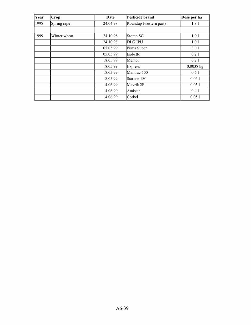
A6-39


1998 Spring rape 24.04.98 Roundup (western part) 1.8 l


24.10.98 DLG IPU 1.0 l

05.05.99 Puma Super 3.0 l

05.05.99 Isobette 0.2 l

18.05.99 Mentor 0.2 l

18.05.99 Express 0.0038 kg

18.05.99 Mantrac 500 0.5 l

18.05.99 Starane 180 0.05 l

14.06.99 Mavrik 2F 0.05 l

14.06.99 Amistar 0.4 l

14.06.99 Corbel 0.05 l

The Danish pesticide leaching assessment programme: Site characterization and monitoring design

Documents

Transcript of The Danish pesticide leaching assessment programme: Site characterization and monitoring design