The Capacity of Wireless Networks

388 IEEE TRANSACTIONS ON INFORMATION THEORY, VOL. 46, NO. 2, MARCH 2000

The Capacity of Wireless NetworksPiyush Gupta, Student Member, IEEE,and P. R. Kumar, Fellow, IEEE

Abstract—When identical randomly located nodes, each ca-pable of transmitting at bits per second and using a fixed range,form a wireless network, the throughput ( ) obtainable by each

node for a randomly chosen destination is�log

bits per

second under a noninterference protocol.If the nodes are optimally placed in a disk of unit area, traffic

patterns are optimally assigned, and each transmission’s range isoptimally chosen, the bit–distance product that can be transportedby the network per second is�( ) bit-meters per second.Thus even under optimal circumstances, the throughput is only� bits per second for each node for a destination nonva-nishingly far away.

Similar results also hold under an alternate physical modelwhere a required signal-to-interference ratio is specified forsuccessful receptions.

Fundamentally, it is the need for every node all over the domainto share whatever portion of the channel it is utilizing with nodesin its local neighborhood that is the reason for the constriction incapacity.

Splitting the channel into several subchannels does not changeany of the results.

Some implications may be worth considering by designers. Sincethe throughput furnished to each user diminishes to zero as thenumber of users is increased, perhaps networks connecting smallernumbers of users, or featuring connections mostly with nearbyneighbors, may be more likely to be find acceptance.

Index Terms—Ad hocnetworks, capacity, multihop radio net-works, throughput, wireless networks.

I. INTRODUCTION

W IRELESS networks consist of a number of nodes whichcommunicate with each other over a wireless channel.

Some wireless networks have a wired backbone with only thelast hop being wireless. Examples are cellular voice and datanetworks and mobile IP. In others, all links are wireless. One

Manuscript received December 3, 1998; revised July 1, 1999. This mate-rial is based on work supported in part by the Air Force Office of ScientificResearch under Contract AF-DC-5-36128, by EPRI and the U.S. Army Re-search Office under Subcontract to Cornell University Contracts WO8333-04and 35352-6086, by the U.S. Army Research Office under Contract DAAH04-95-1-0090, the Office of Naval Research under Contract N00014-99-1-0696,and the Joint Services Electronics Program under Contract N00014-96-1-0129.Any opinions, findings, and conclusions are those of the authors and do not nec-essarily reflect the views of the above agencies.

P. Gupta is with the Department of Electrical and Computer Engineering, andthe Coordinated Science Laboratory, University of Illinois, Urbana, IL 61801USA.

P. R. Kumar is with the University of Illinois at Urbana-Champaign, Coordi-nated Science Laboratory, Urbana, IL 61801 USA.

Communicated by V. Anantharam, Associate Editor for Communication Net-works.

Publisher Item Identifier S 0018-9448(00)01358-4.

example of such networks is multihop radio networks oradhocnetworks. Another possibly futuristic example, see [1], maybe collections of “smart homes” where computers, microwaveovens, door locks, water sprinklers, and other “information ap-pliances” are interconnected by a wireless network.

It is to these types of all wireless networks that this paperis addressed. Such networks consist of a group of nodes whichcommunicate with each other over a wireless channel withoutany centralized control; see Fig. 1. Nodes may cooperate inrouting each others’ data packets. Lack of any centralized con-trol and possible node mobility give rise to many issues at thenetwork, medium access, and physical layers, which have nocounterparts in the wired networks like Internet, or in cellularnetworks.

At the network layer, the main problem is that of routing,which is exacerbated by the time-varying network topology,power constraints, and the characteristics of the wirelesschannel; see Ramanathan and Steenstrup [2] for an overview.The choice of medium access scheme is also difficult inad hocnetworks due to the time-varying network topology and the lackof centralized control. Use of TDMA or dynamic assignment offrequency bands is complex since there is no centralized controlas in cellular networks, FDMA is inefficient in dense networks,CDMA is difficult to implement due to node mobility andthe consequent need to keep track of the frequency-hoppingpatterns and/or spreading codes for nodes in the time-varyingneighborhood, and random access appears to be the currentfavorite. The access problem when many nodes transmit tothe same receiver has been much studied in the literature eversince the genesis of the ALOHA network, and bounds on thethroughput of successful collision-free transmissions as wellas transmission protocols have been devised; see Gallager [3].Sharing channels in networks does lead to some new problemsassociated with “hidden” terminals and “exposed” terminals.The protocols MACA and its extension MACAW, see Karn [4]and Bhargavanet al. [5] respectively, use a series of handshakesignals to resolve these problems to a certain extent. This hasbeen standardized in the IEEE 802.11 protocol, see [6]. At thephysical layer, an important issue is that of power control. Thetransmission power of nodes needs to be regulated so that itis high enough to reach the intended receiver while causingminimal interference at other nodes. Iterative power controlalgorithms have been devised, see Bambos, Chen, and Pottie[7] and Ulukus and Yates [8].

In this paper we analyze the capacity of wireless networks.We scale space and suppose thatnodes are located in a regionof area 1 m2. Each node can transmit at bits per second overa common wireless channel. We shall see that it is immaterial

0018–9448/00$10.00 © 2000 IEEE

GUPTA AND KUMAR: THE CAPACITY OF WIRELESS NETWORKS 389

Fig. 1. Anad hocwireless network.

to our results1 if the channel is broken up into several subchan-nels of capacity bits per second, as long as

Packets are sent from node to node in a mul-tihop fashion until they reach their final destination. They canbe buffered at intermediate nodes while awaiting transmission.

Due to spatial separation, several nodes can make wirelesstransmissions simultaneously, provided there is no destructiveinterference of a transmission by others. We will describe inthe sequel under what conditions a wireless transmission overa subchannel is received successfully by its intended recipient.

We will consider two types of networks,Arbitrary Networks,where the node locations, destinations of sources, and trafficdemands, are all arbitrary, andRandom Networks, where thenodes and their destinations are randomly chosen.

A. Arbitrary Networks: Arbitrarily Located Nodes and TrafficPatterns

In the arbitrary setting we suppose thatnodes are arbitrarilylocated in a disk of unit area in the plane. Each node has an arbi-trarily chosen destination to which it wishes to send traffic at anarbitrary rate; thus the traffic pattern is arbitrary. Each node canchoose an arbitrary range or power level for each transmission.

We need to describe when a transmission is received success-fully by its intended recipient. We will allow for two possiblemodels for successful reception of a transmission over one hop,called theProtocol Modeland thePhysical Model, describedbelow. Let denote the location of a node; we will also use

to refer to the node itself.1) The Protocol Model:Suppose node transmits over theth subchannel to a node Then this transmission is success-

fully received by node if

(1)

for every other node simultaneously transmitting over thesame subchannel.

The quantity models situations where a guard zoneis specified by the protocol to prevent a neighboring node from

1We are grateful to Kimberly King for asking us to be more explicit about theprospects for routing through multiple technologies.

transmitting on the same subchannel at the same time. It alsoallows for imprecision in the achieved range of transmissions.

Another model which is more related to physical layer con-siderations is

2) The Physical Model:Let be the subset ofnodes simultaneously transmitting at some time instant over acertain subchannel. Let be the power level chosen by node

for Then the transmission from a node, ,is successfully received by a node if

(2)

This models a situation where a minimum signal-to-interferenceratio (SIR) of is necessary for successful receptions, the am-bient noise power level is , and signal power decays with dis-tance as We will suppose that , which is the usualmodel outside a small neighborhood of the transmitter.

3) The Transport Capacity of Arbitrary Networks:Givenany set of successful transmissions taking place over time andspace, let us say that the network transports onebit-meterwhenone bit has been transported a distance of one meter towardits destination. (We do not give multiple credit for the samebit carried from one source to several different destinations asin the multicast or broadcast cases). This sum of products ofbits and the distances over which they are carried is a valuableindicator of a network’stransport capacity. (It should be notedthat when the area of the domain is square meters ratherthan the normalized 1 m2, then all the transport capacity resultspresented below should be scaled by Our main resultsare the following. Recall Knuth’s notation:denotes that as well as .

Main Result 1.: The transport capacity of an Arbitrary Net-work under the Protocol Model is bit-meters persecond if the nodes are optimally placed, the traffic pattern is op-timally chosen, and if the range of each transmission is chosenoptimally.

Specifically, an upper bound is bit-meters persecond for every Arbitrary Network for all spatial and temporal


scheduling strategies, while bit-meters persecond (for a multiple of four) can be achieved when thenodes and traffic patterns are appropriately chosen, and theranges and schedules of transmissions are appropriately chosen.

If this transport capacity were to be equitably divided betweenall the nodes, then each node would obtain bit-me-ters per second. If, further, each source has its destination aboutthe same distance of 1 m away, then each node would obtain athroughput capacityof bits per second.

The upper bound on transport capacity does not depend onthe transmissions being omnidirectional, as implied by (1), butonly on there being some dispersion in the neighborhood of thereceiver; see Assumption (A.vi) in Section II.

Main Result 2: For the Physical Model, bit-metersper second is feasible, while bit-meters per secondsis not, for appropriate Specifically,

bit-meters per second (for a multiple of ) is feasible whenthe network is appropriately designed, while an upper bound is

bit-meters per second.

We suspect that an upper bound of order bit-metersper second may actually hold. In the special case where the ratio

between the maximum and minimum powers that trans-mitters can employ is bounded above by, then an upper boundis in fact

bit-meters per second.It is worth noting that both bounds suggest that transport ca-

pacity improves when is larger, i.e., when the signal powerdecays more rapidly with distance.

B. Random Networks: Randomly Located Nodes and TrafficPatterns

In a random scenario, nodes are randomly located, i.e.,independently and uniformly distributed, either on the surface

of a three-dimensional sphere of area 1 m2, or in a diskof area 1 m2 in the plane. Our purpose in studying is toseparate edge effects from other phenomena. Each node has arandomly chosen destination to which it wishes to sendbits per second. The destination for each node is independentlychosen as the node nearest to a randomly located point, i.e., uni-formly and independently distributed. (Thus destinations are onthe order of 1 m away on average.)

In this random setting, we will assume that the nodes arehomogeneous, i.e., all transmissions employ the same nominalrange or power. As for Arbitrary Networks, we will allow forboth a Protocol Model as well as a Physical Model for interfer-ence.

1) The Protocol Model:All nodes employ a commonrangefor all their transmissions. When node transmits to a node

over the th subchannel, this transmission is successfullyreceived by if

i) The distance between and is no more than, i.e.,

(3)

ii) For every other node simultaneously transmitting overthe same subchannel

(4)

2) The Physical Model:All nodes choose a common powerlevel for all their transmissions. Let be thesubset of nodes simultaneously transmitting at some time instantover a certain subchannel. A transmission from a node,

, is successfully received by a node if

(5)

3) The Throughput Capacity of Random Networks:The no-tion of throughput is defined in the usual manner as the timeaverage of the number of bits per second that can be transmittedby every node to its destination.

Definition: Feasible Throughput:A throughput of bitsper second for each node isfeasibleif there is a spatial andtemporal scheme for scheduling transmissions, such that by op-erating the network in a multihop fashion and buffering at in-termediate nodes when awaiting transmission, every node cansend bits per second on average to its chosen destinationnode. That is, there is a such that in every time in-terval every node can send bits to its cor-responding destination node.

Whether a particular throughput level is feasible may dependon the locations of the nodes. These locations are random. Sois the destination for the traffic entering each node. As in PACLearning Theory (see Valiant [9]), given the randomness in-volved in the problem statement, we allow for vanishingly smallprobabilities when defining the “throughput capacity.”

Definition: The Throughput Capacity of Random WirelessNetworks: We say that thethroughput capacityof the class ofRandom Networks is of order bits per second if thereare deterministic constants and such that

is feasible

is feasible

Our main results are the following.

Main Result 3.: In the case of both the surface of the sphereand a planar disk, the order of the throughput capacity is


bits per second for the Protocol Model. For the upper bound weactually prove the sharp cutoff phenomenon that for some

is feasible

Specifically, there are deterministic constantsand notdepending on or such that

bits per second is feasible, and

bits per second is infeasible, both with probability approachingone as Since routing hot spots may form at the centerin the case of a disk on the plane, and yet the order of throughputcapacity is the same as on the surface of the sphere, it shows thatthe cause of the throughput constriction is not the formation ofhot spots, but is the pervasive need for all nodes to share thechannel locally with other nodes.

Main Result 4: For the Physical Model a throughput ofbits per second is feasible, while

bits per second is not, for appropriate both with prob-ability approaching one as Specifically, there aredeterministic constants and not depending onor such that

bits per second is feasible with probability approaching one asIf is the mean distance between two points indepen-

dently and uniformly distributed in the domain (either surface ofsphere or planar disk of unit area), then there is a deterministicsequence not depending on or such that

bit-meters per second is infeasible with probability approachingone as

C. Some Possible Implications

The results in this paper allow for a perfect scheduling al-gorithm which knows the locations of all nodes and all trafficdemands, and which coordinates wireless transmissions tempo-rally and spatially to avoid collisions which would otherwiseresult in lost packets. Also, the nodes are not mobile. If suchperfect node location information is not available, or if nodesmove, or traffic demands are not known, then the capacity canonly be even smaller.

There are some implications of these results which designersmay want to consider. The decrease in throughput withmay beregarded as unacceptable by users when the numberof nodes

is large. Perhaps designers should target their efforts at networksfor smaller numbers of users, rather than try to develop largewireless networks.

A feasible scenario is where nodes need to communicate onlywith nearby nodes. Then the scaled distance between sourcesand destinations is only meters. Thus all nodes cantransmit data to nearby neighbors at a bit rate that does not de-crease with Such a scenario can arise, for example, in collec-tions of “smart homes,” each home having sensors and actuatorscommunicating by wireless means.

Another implication concerns the power consumption byeach node for transmission. Consider Random Networks. Thefraction of time that a modem is busy, whether relaying trafficor sending packets originating at the node, is onlyNot only that, the scaled range of each transmission is about

The bounds for the Physical Model suggest that

a faster rate of decay of signal power with distance, i.e., a larger, allows greater transport and throughput capacity.One more implication follows from the constructive proof

of capacity. It shows that one can group the nodes into smallclusters or “cells,” where in each cell one can designate onespecific node to carry all the burden of relaying multihoppackets, if so desired. Thus a division of labor is possible, werethis to be found profitable. Moreover, it would further reducethe transmission power consumed by the vast majority of othernodes. This may offer some suggestive guidelines for designersof routing protocols.

It should be noted that dividing the channel into subchannelsdoes not change any of the results.

Yet another issue concerns the use of relay nodes.2 Consider aRandom Network with source nodes. Then the throughput that

can be furnished to each of them is only under the

Protocol Model. Suppose additional homogeneous nodes aredeployed as pure relays in random positions, with no indepen-dent traffic needs of their own, i.e., they are not sources. Thenthe throughput that can be furnished to each of thesources is

There is, however, a severe cost of

providing this increase in throughput. The number of additionalrelay nodes that need to be deployed to gain an appreciable in-crease in capacity for the source nodes may be very large. Whenthere are active nodes, to make

equal to five times its value at , will have to be equalto at least . The addition of nodes to serve as pure relaysprovides a less than -fold increase in this term.

One way to overcome the barrier of wireless networks is todo what is done in cellular telephony—connect the base stationsby a wired network. If, however, nondirected wireless links areused for connecting the base stations, then the capacity limita-tion of wireless networks remains with us, though in less ob-vious ways. For example, suppose a high-power base stationis chosen in each cell, which communicates with other distantbase stations by a wireless channel. Then the set of base sta-tions inherits the same capacity limitation. A set ofwire-

2We are grateful to Chip Elliott for raising this issue.


lessly connected base stations can provide a throughput of only

for each base station.

D. A Discussion of the Tradeoffs Involved

Why does the throughput capacity diminish as the number ofnodes increases? For an insight into some of the tradeoffs in-volved, consider Random Networks. Let the mean distance tobe traversed by a packet be, and denote by the commonrange of all transmissions. Then the mean number of hops takenby packets is no less than Thus each node generates at least

bits per second of traffic for other nodes. Since the total

number of nodes is, the total traffic is no less than bitsper second. This has to be served bynodes each capable ofbits per second. Thus one needs An upper bound

on the throughput is therefore Since the term onthe right side grows linearly in , it might appear that to in-crease the throughput by reducing the number of hops traversedby each packet, and thus the burden on other nodes serving asrelays, one should increase the range of each node. How-ever, the expression above is not an achievable upper bound asa function of The reason is that we have neglected the re-duction in capacity due to spatial concurrency constraints, sincenodes close to a receiver are required to be idle to avoid col-lisions which cause the loss of packets. In fact, the loss fromincreasing is quadratic due to the area of the conflict in-volved. Therefore, the desire to reduce the multihop burden andthe desire to increase spatial concurrency and frequency reuseare in conflict. It turns out that when we consider both issues to-gether, we find that one really needs to reduce the value ofto as small a value as possible. However, there is a limit to howsmall one can make When the range of transmissionsis too small, the wireless network loses connectivity. In a pre-cursor result, see [10], the critical range for connectivity of net-works formed by randomly located nodes on a disk in the planehas been determined. Consider the graph with random verticesuniformly and independently distributed in a disk of unit area.Join two vertices by an edge whenever they are within a dis-tance from each other. The critical radius for connectivity

is in the sense that the graph with isconnected with probability approaching one as if andonly if

For Arbitrary Networks under the Protocol model, just threeconstraints—the length of routes, the consumption of valuabletwo-dimensional area by transmissions, and the total number ofnodes—are enough to force the transport capacity to be no morethan bit-meters per second.

The rest of this paper is organized as follows. In SectionII we exhibit upper bounds on the transport capacity of theform bit-meters per second and bit-metersper second, under the Protocol and Physical Models, respec-tively, for Arbitrary Networks. In Section III we show that atransport capacity of bit-meters per second is alsofeasible for Arbitrary Networks. In Section IV we construct ascheduling and routing scheme which achieves a throughput of

bits per second for Random Networks on

In Section V we show that bits per second and

bits per second are upper bounds on the throughput

for Random Networks on under the Protocol and PhysicalModels, respectively. In Section VI we show that the aboveresults for Random Networks also hold for a disk in the plane.

II. A RBITRARY NETWORKS: AN UPPERBOUND ON TRANSPORT

CAPACITY

We consider the setting on a planar disk of unit area. Considerthe following (nearly) minimal set of assumptions:

(A.i) There are nodes arbitrarily located in a disk of unitarea on the plane. (The results carry over to any domainof unit area in which is the closure of its interior.)

(A.ii) The network transports bits over seconds.

(A.iii) The average distance between the source and destinationof a bit is Note that, together with (A.ii), this impliesthat a transport capacity of bit-meters per second isachieved.

(A.iv) Each node can transmit over any subset ofsubchan-nels with capacities bits per second, ,where .

(A.v) Transmissions are slotted into synchronized slots oflength seconds. (This assumption can be eliminated,but makes the exposition easier.)

(A.vi) While retaining the restriction (2) for the case of thePhysical Model, we can either retain (1) in the ProtocolModel or consider an alternate restriction as follows: Ifa node transmits to another node located at a dis-tance of units on a certain subchannel in a certain slot,then there can be no other receiver within a radius ofaround on the same subchannel in the same slot. Thisalternate restriction addresses situations where the trans-missions are not omnidirectional, but nevertheless thereis some dispersion in the neighborhood of the receiver.

Theorem 2.1:i) In the Protocol Model, the transport capacity is

bounded as follows:

bit-meters per second

ii) In the Physical Model


iii) If the ratio between the maximum and minimumpowers that transmitters can employ is strictly bounded aboveby , then



iv) When the domain is of square meters rather than 1 m2,then all the upper bounds above are scaled by

Proof: Consider bit , where Let us sup-pose that it moves from its origin to its destination in a sequenceof hops, where theth hop traverses a distance of Thenfrom (A.iii)

(6)

Note now that in any slot at most nodes can transmit.Hence for any subchannel and any slot

(The th hop of bit is over

subchannel in slot )

Summing over the subchannels and the slots, and noting thatthere can be no more thanslots in seconds, yields

(7)

Consider now the Protocol Model. Suppose that is re-ceiving a transmission from over the th subchannel at thesame time that is receiving a transmission from over thesame subchannel. Then from the triangle inequality and (1)

Similarly,

Adding the two inequalities, we obtain

Hence disks of radius times the lengths of hops centeredat the receivers over the same subchannel in the same slot areessentially disjoint. (Note that this conclusion directly followswhen (1) is replaced by the alternate restriction of Assumption(A.vi)). Allowing for edge effects where a node is near the pe-riphery of the domain, and noting that a range greater than thediameter of the domain is unnecessary, we see that at least aquarter of such a disk is within the domain. Since at mostbits can be carried in slotfrom a receiver to a transmitter overthe th subchannel, we have

(The th hop of bit is over

subchannel in slot ) (8)

Summing over the subchannels and the slots gives

This can be rewritten as

(9)

Note now that the quadratic function is convex. Hence

(10)

Combining (9) and (10) yields

(11)

Now substituting (6) in (11) gives

(12)

Substituting (7) in (12) yields the result.Now turn to the Physical Model. The difference stems from

the need to replace (8) by a different expression. Supposeis transmitting to over the th subchannel at power level

at some time, and let denote the set of all simultaneoustransmitters over the th subchannel at that time. Including thesignal power of also in the denominator, the signal-to-inter-ference requirement (2) for can be written as

Hence

since

Summing over all transmitter-receiver pairs

Summing over all slots and subchannels gives


The rest of the proof proceeds along lines similar to the ProtocolModel, invoking the convexity of instead of

For the consideration of the special case where ,we start with (2). From it, it follows that if is transmitting to

at the same time that is transmitting to , both over thesame subchannel, then

Thus

where Thus the same upper bound as forthe Protocol Model carries over with defined as above.

III. A RBITRARY NETWORKS: A CONSTRUCTIVE LOWER

BOUND ON TRANSPORTCAPACITY

We will now show that the order of the upper bound in theprevious section is sharp for the Protocol Model, by exhibitinga scenario where it is achieved. This scenario is also feasible forthe Physical Model.

Theorem 3.1:There is a placement of nodes and an as-signment of traffic patterns such that the network can achieve

bit-meters per second under the Protocol Model,and

bit-meters per second under the Physical Model, both wheneveris a multiple of

Proof: Consider the Protocol Model. Define

Recall that the domain is a disk of unit area, i.e., of radiusinthe plane. With the center of the disk located at the origin, placetransmitters at locations

and

where is even. Also place receivers at

and

where is odd. Each transmitter can transmit to its nearestreceiver, which is at a distanceaway, without interference fromany other transmitter–receiver pair. It can be verified that thereare at least transmitter–receiver pairs all located within the

domain. (This is done by noting that for a tessellation of theplane by squares of side, all squares intersecting a disk ofradius are entirely contained within a larger concentricdisk of radius The number of such squares is greater than

Now take and ) Restrictingattention to just these pairs, there are a total ofsimultaneoustransmissions, each of range, and each at bits per second.This achieves the transport capacity indicated.

For the Physical Model, a calculation of the SIR shows thatit is lower-bounded at all receivers by Choosing

to make this lower bound equal toyields the result.

The above lower bounds on feasible transport capacity can besharpened. The following bounds may be useful in the design ofnetworks with small numbers of nodes.

Lemma 3.1: In the Protocol Model, there is a placement ofnodes and an assignment of traffic patterns such that the networkcan achieve

bit-meters per second for

bit-meters per second for


for

and

bit-meters per secondfor all

Proof: With at least two nodes, clearly bit-meters persecond can be achieved by placing two nodes at diametricallyopposite locations. This verifies the formula for the bound for

With at least eight nodes, four transmitters can be placedat the opposite ends of perpendicular diameters, and each cantransmit toward its receiver located at a distance to-

ward the center of the domain. This yields bit-metersper second, verifying the formula up to

These bounds can be further improved slightly by tessellatingthe domain into hexagons, at the expense of more unwieldy ex-pressions.

IV. RANDOM NETWORKS: A CONSTRUCTIVELOWER BOUND

ON THROUGHPUTCAPACITY

Now we turn to Random Networks. Even though the settingof the problem is very different, the proof of throughput capacityis somewhat reminiscent of traditional information-theoretic ar-guments. We provide a constructive scheme to show that onecan spatially and temporally schedule transmissions in a randomgraph so that when each randomly located node has a randomlychosen destination, each source–destination pair can indeed beguaranteed a “virtual channel” of capacity bits

per second with probability approachingas , for anappropriate constant We will show how to route traffic


efficiently through the random graph so that no node is over-loaded. The routing scheme will utilize a Voronoi tessellation of

with some special properties. The size of each Voronoi cellis chosen carefully in relation to the number of nodes. Everycell should also be neither too thin nor too fat. The routing willbe over nearly straight-line paths, which assures that it is effi-cient. To show that the load is balanced uniformly over the entirenetwork, we calculate the Vapnik–Chervonenkis dimension forcertain geometrically defined random variables on the plane andthe sphere, which are connected with the tessellations and routesused. We will need to ensure that the routes are independentlyand identically distributed. This will require us to circumventthe possible pitfall that knowledge of one route provides infor-mation on the locations of the source, destination, and interme-diate relay nodes, thus possibly introducing dependencies withother routes which may depend on the locations of these nodes.

We begin the constructive proof of the lower bound on thethroughput capacity for Random Networks. Our treatment willbe directed at the Protocol Model. Where appropriate we willcomment on the arguments required for the Physical Model.

A. A Spatial Tessellation

We use a Voronoi tessellation of the surfaceof the sphere.Recall the definition of a Voronoi tessellation, see Okabe, Bootsand Sugihara [11]. Let be a set of points on

(or any other set for that matter). The Voronoi cell isthe set of all points which are closer tothan to any of the other

’s, i.e.,

Above and throughout, distances are measured on the surfaceof the sphere by segments of great circles connecting two

points; see Stilwell [12]. The point is called the generator ofthe Voronoi cell Fig. 2 shows an example of a tessellationof Unfortunately, the surface of the sphere does not allowany regular tessellation where all cells look the same, except forthe platonic solids; see Lyndon [13]. These latter tessellationscannot be made as fine as we need to make them. Moreover, ourVoronoi tessellations will also need to be not too eccentricallyshaped. We exhibit tessellations with these two special proper-ties in the following lemma, the proof of which is constructive.

Lemma 4.1:For every , there is a Voronoi tessellationof with the property that every Voronoi cell contains a diskof radius and is contained in a disk of radius.

Proof: Denote by a disk of radius centered atChoose as any point in Suppose that have

already been chosen such that the distance between any two’sis at least . There are two cases to consider.

Suppose there is a pointsuch that does not intersectany Then can be added to the collection: Define

Otherwise, we stop.This procedure has to terminate in a finite number of steps

since the addition of each removes the area of a disk of radiusfrom When we stop we will have a set of generators

such that they are at least units apart, and such that all otherpoints on are within a distance of from one of the genera-

Fig. 2. A tessellation of the surfaceS of the sphere.

tors. The Voronoi tessellation arising from this set of generatorshas the desired properties.

In the sequel we will use a Voronoi tessellation for which

(V.i) Every Voronoi cell contains a disk of areaLet

radius of a disk of area on(13)

(Note that the area of a disk of radiusρ on is lessthan ).

(V.ii) Every Voronoi cell is contained in a disk of radius

We will refer to each Voronoi cell as simply a “cell.”

B. Adjacency and Interference

Note that all Voronoi cells are polygons since they are formedas finite intersections of hemispheres on(or halfspaces in thecase of ).

Definition: Adjacent Cells:Say that two cells areadjacent,if they share a common point. (Recall that every cell is a closedset).

Let us choose the range of each transmission so that

(14)

This range allows direct communication within a cell and be-tween adjacent cells.

Lemma 4.2:Every node in a cell is within a distancefrom every node in its own cell or adjacent cell.

Proof: The diameter of cells is bounded by see(V.ii). The range of a transmission is Thus the area cov-ered by the transmission of a node includes adjacent cells.

Definition: Interfering Neighbors:We say that two cells areinterfering neighborsif there is a point in one cell which iswithin a distance of some point in the other cell.


As the name implies, the interpretation is this: If two cells arenot interfering neighbors, then in the Protocol Model a trans-mission from one cell cannot collide with a transmission fromthe other cell.

C. A Bound on the Number of Interfering Neighbors of a Cell

An important property of the constructed Voronoi tessellationis that the number of interfering neighbors of a cell is uni-

formly bounded. This will be exploited in the next section inconstructing a spatial transmission schedule which allows fora high degree of spatial concurrency and thus frequency reuse.From now on ’s will be used to denote deterministic constantsnot depending on

Lemma 4.3:Every cell in has no more than interferingneighbors. depends only on and grows no faster than lin-early in

Proof: Let be a Voronoi cell. If is an interferingneighboring Voronoi cell, there must be two points, one inand the other in , which are no more than unitsapart. From (V.ii), the diameter of a cell is bounded byHence , and similarly every other interfering neighbor in theProtocol Model, must be contained within a common large disk

of radiusSuch a disk cannot contain more than

disks of radius By (V.i), there can therefore be no morethan this number of cells within This therefore is an upperbound on the number of interfering neighbors of the cellTheresult follows from the magnitudes of and chosen asin (14).

D. A Bound on the Length of an All-Cell InclusiveTransmission Schedule

The bounded number of interfering neighbors for each cellallows the construction of a schedule of bounded length whichallows one opportunity for each cell in the tessellation totransmit.

Lemma 4.4:i) In the Protocol Model there is a schedule for transmitting

packets such that in every slots, each cell in the tes-sellation gets one slot in which to transmit, and such that alltransmissions are successfully received within a distancefrom their transmitters.

ii) There is a deterministic constantnot depending on, ,, , or such that if is chosen to satisfy

then for a large enough common power levelthe above resulti) holds even for the Physical Model.

Proof: First we show the result for the Protocol Model.This follows from a well-known fact about vertex coloring ofgraphs of bounded degree: A graph of degree no more thancan have its vertices colored by using no more thancolors, with no two neighboring vertices have the same color;see Bondy and Murthy [14]. One can therefore color the cellswith no more than colors such that no two interfering

neighbors have the same color. This gives a schedule of lengthat most , where one can transmit one packet from eachcell of the same color in a slot.

For the Physical Model we will show that under the sameschedule as above, the required SIR ofis obtained if eachtransmitter chooses an identical power levelthat is highenough, and is large enough.

Note first that any two nodes transmitting simultaneously areseparated by a distance of at least Hence disks ofradius around each transmitter are disjoint. Thearea of each such disk is at least (In the caseof disks on the plane , but it is smaller for disks on thesurface of the sphere).

Consider a node transmitting to a node at a distanceless than The signal power received at is at leastNow we look at the interference power due to all the other si-multaneous transmissions. Consider the annulus of all pointslying within a distance betweenand from A transmitterwithin this annulus has the disk centered at itself and of ra-dius entirely contained within a larger annulusof all points lying between a distance and

The area of this larger annulus is no more than

Each transmitter above “consumes” an area of at least, as noted earlier. Hence the annulus of points at a

distance between and from the receiver cannot containmore than

transmitters. Furthermore, the received power atfrom eachsuch transmission is at most Noting that there can be noother simultaneous transmitter within a distance of

, and taking andfor we see that the SIR at is lower-boundedby

Since , the sum in the denominator converges, and is infact smaller than When is as specifiedand , the lower bound on the SIR converges to a valuegreater than .

E. The Source-Destination Pairs

Each node wishes to communicate with the node nearest to arandomly chosen location. Let be a randomly chosen locationsuch that and are independently and uniformly distributed(i.i.d.) on , and that the sequence is i.i.d. The


destination node for the traffic generated at node ischosen as the node which is closest to

Denote by the straight-line segment connectingandAbove, and in the rest of the paper, by a “straight-line” segmentwe actually mean a segment of the great circle on the surfaceof the sphere; see [12]. There is one significant property enjoyedby the sequence of straight lines

Lemma 4.5:The random sequence of straight-line segmentsis i.i.d.

This has the powerful consequence of allowing us to apply thelaw of large numbers to the i.i.d. straight-line segments. It willbe useful since the route followed by each origination–destina-tion pair will approximate the corresponding straight-line seg-ment, as described in the next section.

F. The Routes of Packets

We will choose the routes of packets to approximate thesestraight-line segments. The straight-line segmentwill inter-sect many cells in the tessellation Let denote the partic-ular cell which contains , and the cell which contains

Packets originating at will be relayed from the cell tothe cell in a sequence of hops. In each hop, the packet istransferred from one cell to another in the order in which theyintersect the line. (If two cells are both “next” cells, then eithercan be chosen arbitrarily). Finally, after reaching the cellcon-taining , the packets will be sent on to their final destination,which we shall show later in Section IV-G to be no more thanone hop away with high probability.

Note that this is a randomized algorithm for choosing routes.It can be thought of as a load balancing scheme with some ratherpowerful uniformity properties, as shown in Section IV-I.

G. Each Cell Contains at Least One Node

To make relaying of traffic from one cell to an adjacent cellfeasible, we need to first ensure thateverycell in con-tains at least one node. For this we use uniform convergencein the weak law of large numbers. Note that uniformity is re-quired over all cells in We recall the following definitions;see Vapnik and Chervonenkis [15] and Vapnik [16]. Letbea set of subsets. A finite set of pointsis said to beshatteredby if for every subset of there is a set such that

TheVC-dimension of , denoted by VC- , isdefined as the supremum of the sizes of all finite sets that canbe shattered by For sets of finite VC-dimension, one has uni-form convergence in the weak law of large numbers.

The Vapnik–Chervonenkis Theorem:If is a set of finiteVC-dimension VC- , and is a sequence of i.i.d.random variables with common probability distribution, thenfor every

whenever

VC-

Fig. 3. Proof that the vertices of a quadrilateral cannot be shattered by the setof disks.

First we will consider the case whereis the set of all diskson the plane. Later we will consider the case where the disksare located on In the planar case we can make use of resultsfrom Euclidean geometry. The following result may perhaps beknown already, though we have been unable to find it in theliterature.

Lemma 4.6:The Vapnik–Chervonenkis dimension of the setof disks in is .

Proof: It is easy to see that there is a three-point set thatcan be shattered by the set of disks. An example is the set ofvertices of an equilateral triangle.

Suppose there is a set of four points that isshattered by the set of disks. If any one of the’s lies in theconvex hull of the other three points, then there is no disk whichcan contain the others without containing too. Hence we canassume without loss of generality that the convex hull of the fourpoints is a quadrilateral.

Again, we obtain a contradiction as follows. Without loss ofgenerality, suppose that the angles of the quadrilateral atand

sum to at least 180, i.e.,

180

Suppose is a disk which contains and , but not or ;see Fig. 3. Extend the diagonal outwards in both directionstill it meets the circumference of at the points andSimultaneously, let and be the points of intersection of thediagonal with the circumference of Then isa cyclic quadrilateral. However,

180

This is a contradiction since the sum of the opposite angles of acyclic quadrilateral is exactly 180.

Now we address the problem of determining the VC-dimen-sion of disks on the surface of a sphere. It is sufficient for us torestrict attention to disks strictly smaller than hemispheres.

To convert results from the plane to , we use a mappingcalled the “inversion map” which maps the punctured surfaceof the sphere onto the plane. Since the radius of the sphere is


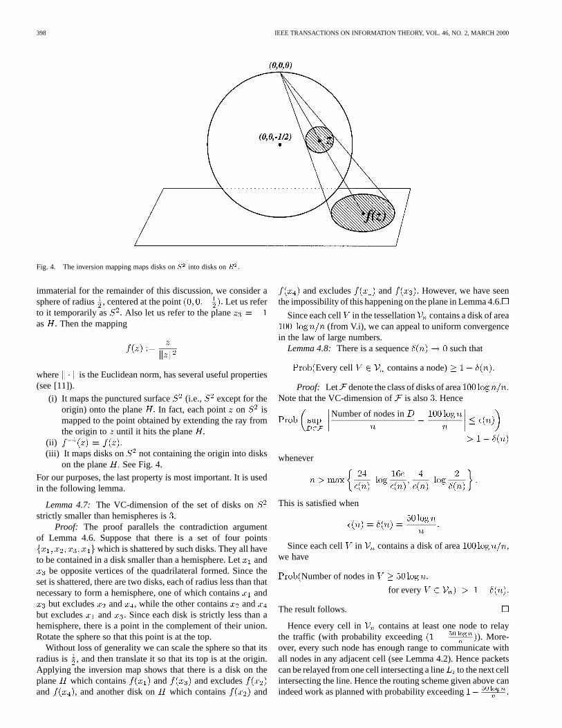
Fig. 4. The inversion mapping maps disks onS into disks onR :

immaterial for the remainder of this discussion, we consider asphere of radius , centered at the point Let us referto it temporarily as Also let us refer to the planeas Then the mapping

where is the Euclidean norm, has several useful properties(see [11]).

(i) It maps the punctured surface (i.e., except for theorigin) onto the plane In fact, each point on ismapped to the point obtained by extending the ray fromthe origin to until it hits the plane

(ii)(iii) It maps disks on not containing the origin into disks

on the plane See Fig. 4.

For our purposes, the last property is most important. It is usedin the following lemma.

Lemma 4.7:The VC-dimension of the set of disks onstrictly smaller than hemispheres is.

Proof: The proof parallels the contradiction argumentof Lemma 4.6. Suppose that there is a set of four points

which is shattered by such disks. They all haveto be contained in a disk smaller than a hemisphere. Letand

be opposite vertices of the quadrilateral formed. Since theset is shattered, there are two disks, each of radius less than thatnecessary to form a hemisphere, one of which containsand

but excludes and , while the other contains andbut excludes and Since each disk is strictly less than ahemisphere, there is a point in the complement of their union.Rotate the sphere so that this point is at the top.

Without loss of generality we can scale the sphere so that itsradius is , and then translate it so that its top is at the origin.Applying the inversion map shows that there is a disk on theplane which contains and and excludesand , and another disk on which contains and

and excludes and However, we have seenthe impossibility of this happening on the plane in Lemma 4.6.

Since each cell in the tessellation contains a disk of area(from V.i), we can appeal to uniform convergence

in the law of large numbers.Lemma 4.8:There is a sequence such that

Every cell contains a node)

Proof: Let denote the class of disks of areaNote that the VC-dimension of is also . Hence

Number of nodes in

whenever

This is satisfied when

Since each cell in contains a disk of area ,we have

Number of nodes in

for every

The result follows.

Hence every cell in contains at least one node to relaythe traffic (with probability exceeding ). More-over, every such node has enough range to communicate withall nodes in any adjacent cell (see Lemma 4.2). Hence packetscan be relayed from one cell intersecting a lineto the next cellintersecting the line. Hence the routing scheme given above canindeed work as planned with probability exceeding


Fig. 5. Transforming great circles intersecting disks into points lying in equatorial bands.

From now on we will use the phrase “with high probability,”abbreviated aswhp to stand for “with probability approaching

as ” The multihop relaying scheme can thereforefunction as plannedwhp.

H. The Mean Number of Routes Served by Each Cell

Recall that the straight line connects and , whereand are independently and uniformly distributed on Byour assumption (V.ii) on the tessellation, each cell is

contained in a disk of radius no more than (Note thatthe area of a disk of radiuson is less than This allowsus to bound the probability that a line intersects a given cell

in

Lemma 4.9:For every line and cell

intersects

Proof: As noted above, from property (V.ii) of the tes-sellation, every cell is contained in a disk of radius

If lies at a distance from the disk, then the

angle subtended at by the disk is no more thanThe area of the sector so formed is no more than If doesnot lie in this sector, then the line joining and cannotintersect the disk containing the cell Hence, for a point at

a distance from the disk of radius containing thecell , the probability that the line connecting and inter-

sects the disk is no more thanSince is uniformly distributed on , the probability den-

sity that it is at a distance from the disk is bounded above by

Integrating, we obtain

intersects

Let denote the great circle containing the line, i.e., theextension of the line so that it wraps around the sphere. Thesame proof technique shows the following.

Lemma 4.10:For every great circle and cell

(Great circle intersects

There being a total of lines , one connecting eachwith , the mean number of lines or great circles passing

through a cell is bounded as follows:

Number of lines in intersecting a cell

Number of great circles in intersecting a cell

I. The Actual Traffic Served by Each Cell

Above, since routes follow lines, we have bounded the meannumber of routes passing through each cell. However, what weneed to bound is theactualrandom number of routes served byevery cell.

To do this we make use of the critical property that the se-quence is i.i.d. Hence, so are the straight linesThis allows us to exploit uniform convergence in the law of largenumbers.

Recall that each cell is contained in a disk of radiusWe will bound the number of great circles intersecting

such disks of radius This is clearly an upper bound on thenumber of lines passing through cells.

We transform the problem of counting “intersections” ofdisks of radius with great circles into a “shattering” problemas follows. For every point on let denote the (unique)great circle containing all points equidistant from it. This isakin to associating an equator with a pole.

Given a great circle , the inverse of this map is not well de-fined since every equator has two poles. However, we arbitrarilychoose one of these two poles and designate it as the inverse

Consider a disk of radius centered at a pointon Let denote the set of all pointswhich are within a distance from ; it is a band of width

around the great circle See Fig. 5.


Let denote the set of all disks on It is easy to see thefollowing lemma and corollary.

Lemma 4.11:The great circle intersects the disk if andonly if the point is contained in the band .

Corollary 4.1: Let denote the set of all great circleswhich intersect The VC-dimension of

is the same as the VC-dimension ofLet denote the set of all disks strictly smaller than

hemispheres. To appeal to uniform convergence in the law oflarge numbers we only have to show that the VC-dimension of

is bounded. Note that for eachband is the intersection of two disks, each strictly largerthan a hemisphere. It is trivial that the VC-dimension of a classof sets is the same as the VC-dimension of the class formed bythe complements of the sets. It is also known (see Vidyasagar[17]) that if is a set of sets, and consists of sets which areeach obtained by intersecting two sets in, then

VC- VC-

Hence we obtain the following lemma.

Lemma 4.12:The VC-dimension of isno more than ten times the VC-dimension of

In Lemma 4.7, we have already shown that the VC-dimensionof is . Hence uniform convergence in the weak law of largenumbers holds, and we obtain the following.

Lemma 4.13:There is a such that

(Number of lines intersecting )

Note that if a cell contains , it needs to forward the packetto its final destination This final destination is at mostone hop away Else, if a cell does not contain , then thetraffic is relayed to the next cell. Hence the traffic handled bya cell is proportional to the number of lines passing through it.Since each line carries traffic of rate bits per second,we have obtained the following bound.

Lemma 4.14:There is a such that

(Traffic needing to be carried by cell)

J. Lower Bound on Throughput Capacity of Random Networks

From Lemma 4.4 we know that there exists a schedule fortransmitting packets such that in every slots, each cellin the tessellation gets one slot to transmit, and such that eachtransmission is received within a range of the transmitter.Thus the rate at which each cell gets to transmit isbits per second.

On the other hand, the rate at which each cellneedsto transmitis less than whp. With high probability, this

rate can be accommodated by all cells if it is less than the rateavailable, i.e., if

Moreover, within a cell, the traffic to be handled by the entirecell can be handled by any one node in the cell, since each nodecan transmit at rate bits per second whenever necessary. Infact, one can even designate one node in each cell as a “relay”node. This node can handle all the traffic needing to be relayed.The other nodes can simply serve as sources or sinks.

We have proved the following theorem, noting the lineargrowth of in in Lemma 4.3, and the choice of inLemma 4.4 for the Physical Model.

Theorem 4.1:(i) For Random Networks on in the Protocol Model, there

is a deterministic constant not depending on , , or ,such that

bits per second is feasiblewhp.ii) For Random Networks on in the Physical Model, there

are deterministic constantsand not depending on, , ,, or , such that

bits per second is feasiblewhp.It should be noted that these throughput levels have been at-

tained without subdividing the wireless channel into subchan-nels of smaller capacity.

V. RANDOM NETWORKS: AN UPPERBOUND ON THROUGHPUT

CAPACITY

Now we turn to the proof of the upper bound on the capacityfor Random Networks.

First we will show that that when the range is too small notevery source will be able to communicate with its desired des-tination.

A. Asymptotic Probability of an Isolated Node

From [10] we know that a necessary condition for connec-tivity whp for the problem of nodes strewn on a disk of unit

area in the plane is , where Thesetting here requires a slightly different treatment. The area

of a disk of radius on is not A saving grace in com-parison to a disk on the plane is that there is no need to considerthe tedious issue of edge effects.

Another subtle issue is that we may not need connectivityof the entire graph. Strictly speaking, we only need that everysource be able to communicate with its chosen destination. Whatwe will show below is that disconnectedness manifests itself bythe presence of isolated nodes. These nodes will then be unable


to communicate with any other node. Hence the absence of iso-lated nodes is indeed a necessary condition for feasibility of anythroughput.

We recall two results from [10].

Lemma 5.1:

(i) For any

(ii) For any given , there exists , such that

for all

If , thenLemma 5.2: If , then, for any fixed

and for all sufficiently large

Given the nodes, denote by the graph whichresults from connecting nodes separated by a distance less than

by an edge. Let denote theprobability that a graph has at least one order-component, i.e., a set of nodes which form a connected set,but which are not connected with any other node. Also, let

denote the probability that is discon-nected.

The main necessary condition for the absence of a single iso-lated node, and consequently also for connectivity, is the fol-lowing.

Lemma 5.3: If where

then

and

Proof: Consider first the case wherefor a fixed Consider , the probability that

hasat leastone order- component. Then

is the only isolated node in

is an isolated node in

and are isolated nodes in

is isolated in

and are isolated in

(15)

Fig. 6. ComputingA(r), the area of a disk of radiusr on a sphere of unitsurface area.

Next we compute the area of a disk of radius onNote that the radius of the sphere itself is From

as indicated in Fig. 6, we get

(16)

Hence

(17)

Now

is isolated in

(18)

Also

and isolated in

(19)

where the first term on the right-hand side above takes into ac-count the case where the distance betweenand is between

and Substituting (18) and (19) in (15) and using(17), we get


Using Lemmas 5.1 and 5.2, for , and any fixedand we have

for all

Now, replace by where Then, for any, for all Also, the probability of

an isolated node is monotone decreasing in. Hence

for Taking limits

Since this holds for all and and since

the results follow.

Corollary 5.1: The asymptotic probability that graphhas an isolated node and is disconnected is strictly

positive if and

B. Upper Bound on Throughput Capacity of Random Networks

The key to the upper bound, as in the case of Arbitrary Net-works, is to note that each transmission consumes valuable area.

Lemma 5.4:The number of simultaneous transmissions onany particular subchannel is no more than

in the Protocol Model.Proof: Suppose node in Fig. 7 transmits successfully to

node on the th subchannel. Then no other node withina distance of can be simultaneously receiving a sep-arate transmission on the same subchannel due to the require-ments (3) and (4) and the triangle inequality.

Hence disks of radius centered at each receiver onthe th subchannel are disjoint. Since the area of each suchdisk is , it follows that the network can support nomore than simultaneous transmissions on thethsubchannel.

Noting that each transmission over theth subchannel is ofbits per second, by adding all the transmissions taking place

at the same time over all the subchannels, we see that theycannot total more than

bits per second in the Protocol Model.Now let denote the mean length of a line connecting two

independently and uniformly distributed points on Then the

Fig. 7. X cannot receive at the same time asX on the same subchannel.

mean length of the path of packets is at least since thereis always a node within a distance of a point on the spherewhp. (This was shown in Lemma 4.8). Thus the mean numberof hops taken by a packet is at least Since each sourcegenerates bits per second, there aresources, and each bit

needs to be relayed on the average by at least nodes, itfollows that the total number of bits per second served by theentire network needs to be at least To ensure thatall the required traffic is carried, we therefore need

Thus

From the previous section we know that is nec-essary to guarantee connectivitywhp. Hence we obtain the fol-lowing upper bound.

Theorem 5.1:For Random Networks on under the Pro-tocol Model, there is a deterministic constant , notdepending on , , or , such that

is feasible

Note that just as in Theorem 4.1 the number of subchannelsis irrelevant.

For the Physical Model, the upper bound is as follows.

Theorem 5.2:For Random Networks on under the Phys-ical Model, there is a deterministic sequence , notdepending on , , , or , such that

Prob is feasible

where is the mean distance between two points independentlyand uniformly distributed on the unit area surface of the sphere.

Proof: In Section II we have shown that bit-meters per second is an upper bound on the transport capacityfor an Arbitrary Network under the Protocol Model. We willnow show that any upper bound on the transport capacity forArbitrary Networks under the Protocol Model is also an upperbound on the transport capacity for Random Networks under thePhysical Model. This will prove the assertion since there arenodes, each having its destination at least meters awayon average.


Consider any set of successful simultaneous transmissionsunder the Physical Model for Random Networks. If is suc-cessfully transmitting to over a the th subchannel, at thesame time that is also successfully transmitting to overthe same subchannel, then from (5)

and so

where Hence any set of simultaneous transmis-sions feasible for Random Networks under the Physical Modelis also feasible in the Protocol Model for Arbitrary Networks.Thus the upper bound on the transport capacity for the latter alsoholds for the former.

VI. THROUGHPUTCAPACITY OF RANDOM NETWORKS ON

PLANAR DISK

The reader may wonder if the capacity is much differentwhen the network is located on a disk in the two-dimensionalplane, rather than on the surface of a sphere. The key issue iswhether hot spots created at the center of the domain by severalorigin–destination pairs routing their traffic through the centerwill make it a bottleneck. The answer is no. The order of thecapacity is unchanged for the Protocol Model, and the earlierorders for the lower and upper bounds for the Physical Modelcontinue to hold.

Clearly, the arguments for the earlier upper bounds stillhold, in view of the same necessary condition on the radius forconnectivity (see [10]) in Random Networks under the ProtocolModel, and the same reduction of Random Networks underthe Physical Model to Arbitrary Networks under the ProtocolModel.

The critical issue is to show that the earlier lower boundscan still be achieved. We show this by using the same tessel-lation-based scheme as on Let be the disk of unit area onthe plane on which the nodes are randomly located. Note thatjust as on , the probability that a randomly chosen line on

intersects a disk of radius is no more thanThis applies even to disks of radius in the center ofThus no unduly hot spots are expected to occur at the center ofthe domain The key result to show however is that with highprobability no hot spots are createdanywhere. That is, we needto show the analog of Lemma 4.13 that the number of lines in-tersecting every cell is less than whp. Lemma 4.11and Corollary 4.1 are not applicable any more since we are noton However, we can circumvent this problem as follows.

We map into a large sphere of radius by using an inver-sion map Consider a straight line on Let denotethe curve on which is the image of the line, and let de-note the corresponding geodesic onconnecting the two endpoints. When is large enough, every such deviates from

by no more than a distance That is, the distortion be-tween the images of straight lines on the disk and the geodesicsis very small.

Consider now a cell of the tessellation of It iscontained in a disk of radius This disk is mapped intoanother disk Let be a disk in withthe same center as, but with a radius larger than that of

It follows that a straight on intersects the disk only ifthe corresponding geodesic on intersects the disk(The reason is that the enlargement of the radius ofaccountsfor the distortion involved in replacing the images of straightline by geodesics). We have already shown in Section IV-I thatthe uniform law of large numbers holds for the probability ofrandomly chosen geodesics intersecting disks. Mapping backinto on the plane shows that the uniform upper bound onthe number of straight lines passing through the disks of radius

applies with high probability.Thus the same results for the capacity continue to hold.

Theorem 6.1:For Random Networks on a planar disk of unitarea, the results of Theorems 4.1, 5.1, and 5.2 continue to hold,except that in Theorem 5.2, is the mean distance betweentwo points independently and uniformly distributed in the planardisk of unit area.

VII. CONCLUDING REMARKS

We have shown that under a Protocol Model of noninterfer-ence, the capacity of wireless networks withrandomly locatednodes each capable of transmitting atbits per second and em-ploying a common range, and each with randomly chosen and

therefore likely far away destination, is This is

true whether the nodes are located on the surface of a three-di-mensional sphere or on a planar disk. Even when the nodes areoptimally placed in a disk of unit area, and the range of eachtransmission is optimally selected, a wireless network cannotprovide a throughput of more than bits per secondto each node for a distance of the order of 1 m away. In fact,summing over all the bits transported, a wireless network on adisk of unit area in the plane cannot transport a total of morethan bit-meters per second, irrespective of how theload is distributed. Under a Physical Model of noninterference,the lower bounds are the same as those above for the ProtocolModel, while the upper bounds on throughput are for

Random Networks and for Arbitrary Networks.Splitting the channel into several subchannels does not

change any of these results.These results have some implications that designers may want

to consider. Perhaps efforts should be targeted at designing net-works with small numbers of nodes.

On the positive side, the results show that modulo furthermedium access or adaptive routing restrictions, communicationwith nearby neighbors at constant bit rates can be provided in adense clusters of nodes, since the source–destination distancesthen shrink in scaled length as This shows that sce-narios envisaged in collections of smart homes, or networks withmostly close-range transactions and sparse long-range demands,are feasible.

We have not considered in this paper the additional burden incoordinating access to the wireless channel, and the additional


burden caused by mobility and link failures and the consequentneed to route traffic in a distributed and adaptive way. Thesecan only further throttle capacity. It would be useful to quantifythese additional burdens.

Another issue to be studied is delay. This will arise when thetraffic is bursty or when nodes are mobile. These two sources ofdelay are markedly different.

Finally, spatial directivity in the antennas or beamformingwill be advantageous in increasing the spatial concurrencyof transmissions, since wireless networks can then behavelike wired ones. Ephremides [18] has analyzed the mediumaccess problem for a single channel and shown that when onlyternary feedback from the channel can be used to scheduletransmissions, the throughput of collision-free successfultransmissions is the same as in the usual omnidirectional case.When node locations and demands are known and do not haveto be figured out purely from ternary feedback, transmissionscan be advantageously scheduled so that collisions are avoided,and the throughput can consequently be increased. However,this is a challenging proposition since transmissions from nodeswill have to be carefully orchestrated. Such schemes may posesome technological challenges though for low-cost networks.Finally, there is the challange of a more information-theoreticformulation.

REFERENCES

[1] “What you will want next and the really smart house,”Newsweek, May30, 1999.

[2] S. Ramanathan and M. Steenstrup, “A survey of routing techniques formobile communication networks,”Mobile Networks and Appl., vol. 1,no. 2, pp. 89–104, 1996.

[3] R. Gallager, “A perspective on multiaccess channels,”IEEE Trans. In-form. Theory (Special Issue on Random Access Communications), vol.IT-31, Mar. 1985.

[4] P. Karn, “MACA: A new channel access method for packet radio,” inProc. 9th Computer Networking Conf., Sept. 1990, pp. 134–140.

[5] V. Bharghavan, A. Demers, S. Shenkar, and L. Zhang, “MACAW: Amedia access protocol for wireless LANs,” inProc. SIGCOMM’94Conf. on Communications Architectures, Protocols and Applications,Aug. 1994, pp. 212–225.

[6] Wireless LAN Medium Access Control (MAC) and Physical Layer (PHY)Specifications, IEEE Standard 802.11–1997, IEEE Computer SocietyLAN MAN Standards Committee, Ed., 1997.

[7] N. Bambos, S. Chen, and G. Pottie, “Radio link admission algorithmsfor wirelessd networks with power control and active link quality pro-tection,” inProc. IEEE INFOCOM, Boston, MA, 1996.

[8] S. Ulukus and R. Yates, “Stochastic power control for cellular radio sys-tems”, Preprint, 1996.

[9] L. Valiant, “A theory of the learnable,”Commun. ACM, vol. 27, pp.1134–1142, Nov. 1984.

[10] P. Gupta and P. R. Kumar, “Critical power for asymptotic connectivityin wireless networks,” inStochastic Analysis, Control, Optimization andApplications: A Volume in Honor of W. H. Fleming, W. M. McEneany, G.Yin, and Q. Zhang, Eds. Boston, MA: Birkhauser, 1998, pp. 547–566.

[11] A. Okabe, B. Boots, and K. Sugihara,Spatial Tessellations Concepts andApplications of Voronoi Diagrams. New York: Wiley, 1992.

[12] J. Stilwell,Geometry of Surfaces. New York: Springer-Verlag, 1992.[13] R. C. Lynwood,Groups and Geometry. Cambridge, U.K.: Cambridge

Univ. Press, 1985.[14] J. A. Bondy and U. Murthy,Graph Theory with Applications. New

York: Elsevier, 1976.[15] V. N. Vapnik and A. Chervonenkis, “On the uniform convergence of

relative frequencies of events to their probabilities,”Theory Probab. itsApplic., vol. 16, no. 2, pp. 264–280, 1971.

[16] V. N. Vapnik, Estimation of Dependences Based on EmpiricalData. New York: Springer-Verlag, 1982.

[17] M. Vidyasagar,A Theory of Learning and Generalization. London,U.K.: Springer-Verlag, 1997.

[18] A. Ephremides, “Some wireless networking problems with a theoreticalconscience,” inCodes, Curves, and Signals: Common Threads in Com-munications, A. Vardy, Ed., Aug. 1998.

The Capacity of Wireless Networks

Documents

Transcript of The Capacity of Wireless Networks