The awakening of Attneave's sleeping cat: Identification of everyday objects on the basis of...

1 IntroductionA skilled draughtsman needs only a few well-selected line segments to depict an everydayobject. Our ancestors interpreted some cracks in the rocks as representations of (partsof) a familiar object (eg a mammoth) and added a few markings to strengthen theimpression (Halverson 1992). Humans are so good at identifying objects in line drawingsthat it must tell something about the way the visual system extracts and processes theessential information for object identification from the more natural visual stimulation.Computer vision systems, on the other hand, have the greatest difficulties in processingnew images of objects, even when they have stored several related images in their data-base. This glaring contrast has inspired research into the information available in linedrawings (eg Koenderink and van Doorn 1982).

More than half a century ago, Attneave (1954) argued that the information aboutobject shape is not distributed homogeneously in an image but is concentrated atcontours (where the continuous distribution of spectral or grey-level values is usuallythe sharpest) and furthermore, that information along the contour is concentratedat points where the curvature reaches extreme values (curvature extrema). He usedtwo demonstrations to support his intuition about the role of curvature extrema. Inone demonstration, he asked participants to mark salient points along the contour of arandom shape, and showed that the frequency plots were centred on the curvatureextrema (see figure 1a). In a second demonstration, which has become known asAttneave's sleeping cat (see figure 1b), he created a version of a line drawing of hissleeping cat by connecting the curvature extrema by straight lines. The fact that this

The awakening of Attneave's sleeping cat: Identificationof everyday objects on the basis of straight-line versions ofoutlines

Perception, 2008, volume 37, pages 245 ^ 270

Joeri De Winter, Johan WagemansôLaboratory of Experimental Psychology, University of Leuven, Tiensestraat 102, B 3000 Leuven,Belgium; e-mail: [email protected] 21 February 2005, in revised form 31 May 2007; published online 22 February 2008

Abstract. Attneave (1954 Psychological Review 61 183 ^ 193) demonstrated that a line drawing ofa sleeping cat can still be identified when the smoothly curved contours are replaced bystraight-line segments connecting the positive maxima and negative minima of contour curvature.Using the set of line drawings by Snodgrass and Vanderwart (1980 Journal of ExperimentalPsychology: Human Learning and Memory 6 174 ^ 215) we made outline versions (with knowncurvature values along the contour) that can still be identified and that can be used to testAttneave's demonstration more systematically and more thoroughly. In five experiments (with444 subjects in total), we tested identifiability of straight-line versions of 184 stimuli with differentselections of points to be connected (using 24 to 28 subjects per stimulus per condition).Straight-line versions connecting curvature extrema were easier to identify than those based oninflections (where curvature changes sign), and those connecting salient points (determined by161 independent subjects) were easier than those connecting midpoints. However, identificationvaried considerably between objects: some were almost always identifiable and others almostnever, regardless of the selection criterion, whereas identifiability depended on the specific shapeattributes preserved in the straight-line version of the outline in other objects. Results are dis-cussed in relation to Attneave's original hypotheses as well as in the light of more recent theorieson shape perception and object identification.

doi:10.1068/p5429

ôAuthor to whom all correspondence should be addressed.

straight-line version was still easy to recognise, showed that the continuous curvaturechanges along the contour are not important and that the critical information aboutshape is located at curvature extrema.

Attneave's intuition has sparked a lot of interest in several areas of research.Resnikoff (1985) formalised the notion of information using classic measures frominformation theory and has provided mathematical proof of information concentrationat curvature extrema. More recently, Feldman and Singh (2005) proposed an alterna-tive quantification scheme and extended Attneave's original idea by showing that thesame logic implies that negative curvature extrema (minima) must be more informativethan positive curvature extrema (maxima). The reason is that all natural objects aremore convex than concave and closed contours must, therefore, always turn inwardsagain after they have turned away from the object centre.

Attneave's demonstration about the salience of curvature extrema in random shapes(based on an unpublished study on 16 similar random shapes with 80 participants)has received further empirical support from a study on 12 silhouettes of sweet potatoeswith 12 participants (Norman et al 2001). Using contour versions derived from theset of 260 line drawings of everyday objects by Snodgrass and Vanderwart (1980), wehave obtained salience data from 161 participants, which appear in a separate paper(De Winter and Wagemans 2008). Attneave's anecdotal demonstration with the sleep-ing cat still awaits experimental confirmation when applied to other everyday objects.

There are several good reasons, both theoretical and empirical ones, for performinga more thorough study inspired by Attneave's sleeping cat. First, it is not clear howAttneave selected the salient curvature extrema to be connected by straight lines. It ishighly unlikely that he did so using mathematical techniques. He probably relied onhis own intuitions as a keen observer. In fact, it is quite likely that Attneave didnot even start from a line drawing with continuously curved lines but immediatelydrew the straight-line version while he was watching his sleeping cat (see footnote 2in Feldman and Singh 2005). Selecting curvature extrema is not a trivial matter.Mathematically, there is a local curvature extremum whenever a curvature value issurrounded by two segments of larger or smaller curvature values. When the contouris traced and its corresponding curvature values are plotted in a so-called curvaturegraph, all curvature singularities can be located with mathematical precision (see fig-ure 2). It is useful to distinguish between three types of curvature singularities: positivemaxima (M�), negative minima (mÿ), and inflections (I), points where the curvature

(a) (b) (c)

Figure 1. (a) First demonstration by Attneave (1954) of the importance of curvature extrema: peoplemark them as more salient points along the contour of a random shape (higher frequency isrepresented by a longer line). (b) Second demonstration by Attneave (1954) of the importanceof curvature extrema (known as Attneave's sleeping cat). A sleeping cat can still be identified ina straight-line version connecting the curvature extrema, removing all the continuous curvaturealong the contour. (c) Lowe's (1985) variation in which midpoints between curvature extremaare connected by straight-line segments.

246 J De Winter, J Wagemans

Straigh

t-lineversio

nsof

object

outlin

es247

N:/psfiles/per3702w

/

�

ÿ

Curvature

mÿ I M�

Figure 2. An example of a smoothly curved contour derived from a line drawing of an anchor by Snodgrass and Vanderwart (1980).Superimposed on the contour are the curvature singularities: local maxima of curvature or positive maxima (M�) are marked by squares,local negative minima of curvature or negative minima (mÿ) are marked by triangles, and zero crossings or inflections (I) are markedby circles. Below the outline, the curvature of the outline is plotted with the starting point indicated on the outline (the contour is tracedin counterclockwise direction). The same curvature singularities are also marked on the curvature graph (with the same symbols).

changes sign and goes through zero. The example in figure 2 shows clearly that manyof the local curvature extrema are not salient (they are sometimes even located onwhat looks like a straight-line segment). This observation necessitates the use of ajustifiable selection criterion, which Attneave did not specify. In contrast, we testedand compared several ones. The more general issue of how to define curvature (andcurvature extrema) at different spatial scales and how to select the most relevant per-ceptual ones falls outside the scope of the present study (see Lowe 1988; Witkin 1986;and appendix 4 in De Winter and Wagemans 2006).

Second, Attneave did not use a control condition in which other points were con-nected by straight lines. Lowe (1985) showed that a straight-line version formed byconnecting midpoints (points halfway between extrema) is also easy to identify (seefigure 1c). Moreover, Biederman (1988) tested several variants of line drawings of cats(including figures 1b and 1c) and showed that error rates and correct naming timesvaried considerably, even between those that appeared easy to recognise (eg from 17%and 1078 ms for figure 1b and 39% and 939 ms for figure 1c, to about 700 ms and noerrors for normal line drawings).

Third, in line with Lowe's sleeping cat, Kennedy and Domander (1985) showedthat points halfway between corner points (midpoints) are more informative thancorner points, and that points halfway between midpoints and corner points are evenmore informative still. They used short line segments rather than single points (forwhich they have been criticised by Deregowski 1986) and fragmented versions may bequite different than straight-line versions because additional processes like filling-income into play (see also Panis et al 2008). Nevertheless, there are good mathematicalreasons to believe that inflections (often close to midpoints between extrema) are per-ceptually important too: a change in curvature sign is easier to compute, more robust,and more stable under transformations than maxima or minima of curvature (Van Goolet al 1994) and inflections on the contour correspond to parabolic lines on the 3-D objectsurface, separating convex and concave surface regions (Koenderink and van Doorn1982). In other words, comparing straight-line versions connecting curvature extremawith straight-line versions connecting other points is not just interesting for the sake ofcomparison; it is also theoretically meaningful.

For all these reasons, we have embarked upon a large-scale study, consisting ofseveral experiments, in which we have tested Attneave's idea about the role of curva-ture extrema for object identificationöas demonstrated with his sleeping catöusingmuch larger sets of stimuli and groups of participants. We have created silhouette andcontour versions of the famous Snodgrass and Vanderwart (1980) set of line drawingsof everyday objects and we have determined identification norms for them (Wagemanset al 2008; see also appendix in Wagemans et al 1998). Because we have continuouscurvature values along these contours, we can also examine whether segmentationsof these stimuli confirm segmentation rules like the minima rule by Hoffman andRichards (1984; see De Winter and Wagemans 2006), whether fragmented versionsare indeed easier to recognise with fragments around inflections than around extrema,as suggested in the study by Kennedy and Domander (1985; see Panis et al 2008), andwhether curvature extrema are more salient than other points, as suggested by Attneave'sfirst demonstration (figure 1a) and confirmed by a more thorough study with randomshapes (Norman et al 2001; see De Winter and Wagemans 2008). The study withstraight-line versions which we present here is, therefore, part of a larger researchprogram on the role of curvature singularities in shape and object perception (foran overview, see De Winter and Wagemans 2004), which provides interesting bench-mark data to test several theoretical proposals, both from perceptual psychology andcomputer vision.


2 General methodsBecause all five experiments reported here belong to the same large-scale study, theyshare several aspects of the methods for data acquisition (eg subjects, stimuli, proce-dure) and data analysis (eg scoring, dependent variables, a posteriori analyses). To avoidrepetition in the description of the individual experiments, we include these generalaspects of the methods here, and focus on the specific details in which the methodsdiffer between experiments below. We will also use tables to make it easier to maintainan overview of the differences and similarities between the experiments.

2.1 SubjectsFirst-year psychology students at the University of Leuven participated in all experi-ments in this study as a mandatory component of their curriculum. They were alwaysnaive regarding the purpose of the experiment and unfamiliar with the stimuli (weused different samples with new freshmen in each of four consecutive academic years).Depending on the number of conditions in each experiment, we used a different num-ber of subjects to have data from 20 to 30 subjects per stimulus per condition withina reasonable time per subject (about 20 min).

2.2 StimuliThe stimulus set consisted of 184 straight-line versions derived from the 260 linedrawings of everyday objects by Snodgrass and Vanderwart (1980). In a previous large-scale study (Wagemans et al 2008; see also De Winter and Wagemans 2004), we madesilhouette and contour versions of the complete Snodgrass and Vanderwart set. First,silhouettes were made by filling-in the interior surfaces in black. Their outlines werethen extracted automatically and spline-fitted to obtain smooth curvature values at allpoints along the contour. We then determined the degree of identifiability in a groupof 356 subjects. Not all of these outlines were equally easy to identify (range between0% and 100%), and because we expected that the identifiability would be poorer forthe straight-line versions to be tested here, we selected only those that were stillreasonably identifiable as a silhouette. The lower limit was set to 20%, meaning thatthe silhouette was still named correctly by 20% of the subjects in the previous study.Based on this criterion, 66 outlines were excluded.

Some additional outlines were excluded from the remaining 194 ones for the follow-ing reasons: (i) Outlines that are completely convex have no inflections and thereforecannot be used in one of the two conditions (see below). Based on this criterion, 6 out-lines were excluded (eg ball, barrel). (ii) Because of the spline-fitting procedure, someoutlines had some small anomalies in the outline shape (eg small local distortions atthe vertices) and they were excluded because these anomalies could have affected thestraight-line versions differentially and hence our major results of interest. Based onthis criterion, 3 outlines were excluded (bee, broom, needle). (iii) To be able to dividethe number of stimuli into equal subgroups, we excluded one additional outline withlow identifiability (telephone). These selection criteria led to a set of 184 stimuli (out of260), with an average identification rate of 87.3% (SD � 19:4%). The consequenceof using this subset from the Snodgrass and Vanderwart (1980) set of stimuli is thatour results concern identification based on 2-D outlines of everyday 3-D objects. Weassume that the original Snodgrass and Vanderwart line drawings capture the 3-Dstructure of their objects as well as possible but we cannot say anything about theidentifiability of straight-line versions that would be derived from non-canonical views.

From the smooth contours obtained from the spline-fitted outlines, we extractedparticular curvature singularities (using different selection criteria in the differentexperiments) and we connected them by straight lines, as Attneave (1954) may havedone to create his sleeping cat. In experiments 1, 2, and 3, we compared straight-lineversions connecting extrema (as Attneave did in figure 1b) with straight-line versions

Straight-line versions of object outlines 249

connecting inflections (often close to halfway between extrema, as Lowe did in figure 1c).In experiments 4 and 5, we started from salient points as determined empirically fromanother large-scale study with an independent group of 161 subjects (De Winter andWagemans 2008). In experiment 4, we then selected the most salient points and con-nected either these points by straight lines or points halfway between them (midpoints).In experiment 5, we created another variant based on the midpoints. In all of thestimuli used in the present study, we filled the interior surface of these straight-lineversions with light-grey (75% of maximum luminance) to create silhouettes (see figures4, 7, 8, and 9 for examples). We make these stimuli available on our website, alongwith their identifiability in their silhouette version as well as in the versions tested here(see http://ppw.kuleuven.be/labexppsy/johanw/wag 2D.htm).

Half of the straight-line stimuli presented to a subject were constructed with pointsof one type (extrema or salient points), and the other half of the stimuli with points of thecomplementary type (inflections or midpoints). The assignment of stimuli to conditionswas always counterbalanced between subjects. The two groups of stimuli were alwaysmatched to have approximately the same average identifiability, the same number of livingversus non-living objects, and the same average number of inflections.

2.3 ProcedureThe experiments were performed in a computer classroom with 33 PCs separated byabout 1 m. There were usually multiple sessions with a maximum number of 30 subjectsper session. We presented all the stimuli centred on a 17 inch CRT display at a view-ing distance of approximately 0.7 m. The display resolution was set to 1024 by 768pixels and a refresh rate of 60 Hz. Stimuli were all contained within a box of 6406480 pixels (not drawn as such), for a maximum viewing angle of 16.3 deg by 12.2 deg.

Each straight-line version was presented for a maximum of 5 s and then replacedby a fixation cross. Subjects were asked to identify each stimulus and subsequentlyinput the name via the computer keyboard and click on an OK button when finished.Subjects could begin typing the name of the object as soon as they had identified thestimulus and they could type and correct as long as they wanted. If the subject clickedon OK in a time period shorter than 5 s, the stimulus was removed from the screenand the next stimulus appeared. The presentation order was randomised for eachsubject separately and the experimenter secured silence throughout the session until hefinished with the last subject.

2.4 ScoringIn the previous study with silhouettes and outlines (Wagemans et al 2008; see alsoDe Winter and Wagemans 2004), we used two criteria to score the responses as cor-rect or incorrect. With the more stringent criterion, a response was counted as correctonly when the name given was the same as that listed by Snodgrass and Vanderwart(1980). With the more liberal criterion, synonyms and colloquial names that clearlyindicated the same concept were also considered correct. However, remotely relatednames that were referring to different basic-level categories (eg `̀ dog'' for `̀ fox'' or `̀ fly''for `̀ bee'') were not allowed. Because we used Flemish subjects in all of our experimentsand Flemish has many more synonyms and colloquial names than English or Dutch(eg Severens et al 2005), we decided to use the more liberal criterion in the presentstudy (as well as in the related ones by De Winter and Wagemans 2008 and Panis et al2008). It is the best measure of basic-level identification. Scoring was done automaticallyfor all names that were already in our database from the previous study. New names werescored manually by applying the same criteria (in the case of doubt, the two authorsdecided jointly). The database was updated with the new names (and their scoring) eachtime a new experiment was performed. All experiments in this study used the samescoring criteria and the results are therefore comparable across the different experiments.


2.5 Data analysisWe determined the average percentages of correct identification in each conditionand compared them with a t-test when there were only two conditions, or an analysisof variance (ANOVA) when there were more than two conditions. Because we believe thatour data set may also be used as a benchmark to test specific models of object recognition(particularly computer vision or pattern recognition models), we also made available onour website the identification rates of all of the individual stimuli in all of the differentversions of this study (see http://ppw.kuleuven.be/labexppsy/johanw/wag 2D.htm).

As a first step in an exploratory analysis of the factors determining identificationof straight-line versions, we determined the stimulus difference between the straight-line version and the original outline version for all stimuli, and correlated performancewith it. The stimulus different was quantified as follows (see figure 3 for an example).First, the original silhouette was drawn in black, the straight-line version was drawnin white, and the two versions were overlaid, so that the difference in overlap in onedirection was then visible in black. The area of the difference was then calculated asthe number of black pixels. Next, the same procedure was repeated, but now thestraight-line version was drawn in black and the original version in white and the areain this direction of the difference was also calculated. Finally, the total stimulus differ-ence computed in this way was the sum of the two black areas remaining after applying

Type Contour/Overlap

Original

SP100

Original ÿ SP100

SP100 ÿ Original

{Original ÿ SP100}

�{SP100 ÿ Original}

Figure 3. Stimulus difference between the straight-line versions and the original outlines wasquantified as the total area of the nonoverlappingparts. The three-step procedure is illustratedhere for the straight-line version of the airplanein experiment 4 (connecting salient points).First, we calculated the area of the originaloutline (Original) minus the overlapping areaof the straight-line version (SP100), resultingin the black parts shown in `Outline ÿ SP100'.Second, we calculated the area of the straight-line version (SP100) minus the overlapping areaof the original outline (Original), resulting inthe black parts shown in `SP100 ÿ Outline'.Third, the two black areas were added.


the overlay-and-subtract procedure in both directions. To avoid area differences in theoriginal outlines affecting the results, this deviation measure was then divided bythe original outline area. We could then correlate the relative stimulus difference foreach condition with the decrease in identification rate in that condition.

We also computed other stimulus measures (contour length, number of cornerpoints, contour length divided by the number of corner points, average length of allthe straight-line segments, variability of it, etc) and correlated performance with them.However, we generally obtained weak correlations. Therefore we are not reportingthem here because they did not help us in explaining the differences in identificationrate. In section 8 we include some of our observations from these exploratory analyses,as an illustration of the potential of this approach. All our stimuli have also been madeavailable on our website (both as bitmaps and as pixel files) so that anyone with partic-ular ideas about relevant stimulus variables determining identification can test them onour benchmark data sets (see http://ppw.kuleuven.be/labexppsy/johanw/wag 2D.htm).

3 Experiment 1: Curvature singularitiesöone extremum per lob3.1 IntroductionIn the first three experiments, curvature singularities were corner points connected bystraight-line segments. They differed only in the way the curvature singularities wereselected. In experiment 1, we selected only one curvature extremum for each segmentof the contour with a particular sign of curvature: one maximum (M�) per segment ofpositive curvature and one minimum (mÿ) per segment of negative curvature.

3.2 MethodsThe aspects of the methods common to all of the experiments have been reportedin section 2, above. Here, we describe only the specific aspects of the methods that areunique to this experiment (see table 1 for an overview).

3.2.1 Subjects. 56 participants (13 male, 43 female, mean age 19.3 years) were tested intwo sessions with a maximum number of 30 participants in each session.

3.2.2 Stimuli. The two conditions in this experiment consisted of straight-line versionsconnecting either curvature extrema (E) or inflections (I). Each outline contour in ourset of stimuli had more extrema than inflections. To make sure that the number ofpoints to be connected was equal in both conditions, we used the following criterionto select extrema. Within a fragment of positive or negative curvature (called here alob), we selected the extremum with the highest absolute curvature. This automaticallyresults in an equal number of extrema and inflections per outline, because each lob withpositive curvature is followed by a lob of negative curvature (and vice versa), with aninflection point inbetween. The mean number of selected points across stimuli was 29.7(median � 24:5). Stimulus examples are shown in figures 4, 7, and 8.

Table 1. Methodological details of the five experiments.

Experiment

1 2 3 4 5

Number of subjects 56 50 206 108 24

Number of stimuli 184 184 184 184 142

SP100 vs MP100Stimulus conditions E vs I E vs I E vs ISP75 vs MP75

MPT

Number of stimuli per subject 184 184 46 184 142

Number of subjects 28 25 26 27 24per stimulus per condition


Straigh

t-lineversio

nsof

object

outlin

es253

Group Experiment 1 Experiment 2 Experiment 3 Experiment 4 Experiments 4 and 5

E I E I E I SP100 MP100 SP100 MPT

4

�

5

96% 0% 100% 0% 96% 4% 96% 4% 56% 38%

78% 78% 100% 100% 100% 100% 100% 100% 100% 100%

86% 96% 28% 88% 41% 60% 0% 22% 15% 92%

Group Experiment 1 Experiment 2 Experiment 3 Experiment 4 Experiments 4 and 5

E I E I E I SP100 MP100 SP100 MPT

4

�

5

96% 0% 100% 0% 96% 4% 96% 4% 56% 38%

78% 78% 100% 100% 100% 100% 100% 100% 100% 100%

86% 96% 28% 88% 41% 60% 0% 22% 15% 92%

Figure 4. Examples of straight-line versions of the Snodgrass and Vanderwart (1980) pictures, constructed by connecting a number of curvatureextrema (E) or salient points (SP), inflections (I) or midpoints (MP). On the basis of the identification rates in the different conditions, wedistinguish between three groups: in the group in the first row (4), the E or SP version is identified better than the I or MP version. In thegroup in the second row (�) both versions are identified equally well. In the group in the third row (5), the I/MP version is identified betterthan the E/SP version. Below each example is the identification rate (in %) for that particular stimulus.

3.2.3 Procedure. Each subject received all 184 stimuli, half of them in E version andhalf in I version (stimulus assignment was counterbalanced across subjects). Each stim-ulus was thus presented to 28 subjects per condition.

3.3 Results and discussionThe most important identification results are tabulated: separately per conditionin table 2 (see over), and comparatively between conditions in table 3. Some stimulusmeasures that might correlate with identifiability are included in table 4. The distribu-tion of identification rate in the two conditions is plotted in figure 5a.

Identification was still reasonable or good for the straight-line versions connectingthe extrema (E versions), but it was rather poor for the straight-line versions con-necting the inflections (I versions). Mean and median identifications were 46.4% and41.1% for E versions and 20.4% and 3.6% for I versions (see table 2). A t-test on themeans revealed a large statistical difference between the two conditions: t366 � 7:28,p 5 0:001. The fact that E versions can still be identified in many cases (eg 50 arewithin 10% of the identification rate of the original outlines) supports Attneave's (1954)idea that continuous curvature changes are often not needed. Moreover, the fact thatE versions are easier to identify than I versions confirms that Attneave's version ofthe sleeping cat (figure 1b) was more representative of everyday objects than Lowe'sversion (figure 1c). However, there was a considerable range of identification per-formance across the stimuli (see figure 5a): there are relatively more E versions withhigh identification rates (eg 470%) than I versions, and more I versions with loweridentification rates (eg 530%) than E versions, but in both versions identifiability isdistributed across the whole range from 0% to 100%. This stimulus variability may beinformative about stimulus variables affecting identifiability.

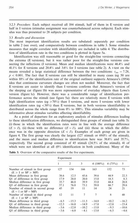
As a point of departure for an exploratory analysis of stimulus differences leadingto these identification differences, we distinguished three groups of stimuli (see table 3):(i) those in which the identification rates were in line with the average difference(E 4 I), (ii) those with no difference (E � I ), and (iii) those in which the differ-ence was in the opposite direction (E 5 I ). Examples of each group are given infigure 4. The first group was clearly the largest (127 stimuli or 69.0% of the stimuli),and the mean and median difference in identification here was 38.6% and 35.7%,respectively. The second group consisted of 45 stimuli (24.5% of the stimuli), 41 ofwhich were not identified at all (0% identification in both conditions). Many of the

Table 3. Overview of the comparative results of the five experiments.

Experiment

1 2 3 4 (100%) 4 (75%) 5

Number of stimuli in first group 127 154 166 163 152 73(E 4 I or SP 4 MP)

Mean difference in first group 38.6 12.5 45.6 39.6 44.9 22.3Q1 of difference in first group 17.9 20.0 20.0 15.0 18.5 8.3Median difference in first group 35.7 46.0 39.9 33.0 44.4 20.8Q3 of difference in first group 57.1 76.0 73.1 59.0 66.7 29.6Number of stimuli in second group 45 19 11 14 24 21(E � 1 or SP �MP)

Number of stimuli in third group 12 11 7 7 8 48(E 5 1 or SP 5 MP)

Mean difference in third group ÿ6.5 ÿ15.3 ÿ11.5 ÿ14.8 ÿ10.2 ÿ16.2Q1 of difference in third group ÿ12.5 ÿ16.0 ÿ14.9 ÿ17.0 ÿ12.0 ÿ23.4Median difference in third group ÿ3.6 ÿ12.0 ÿ10.2 ÿ15.0 ÿ9.3 ÿ10.6Q3 of difference in third group ÿ3.6 ÿ6.0 ÿ4.1 ÿ13.0 ÿ6.5 ÿ4.6


Table 2. Overview of the identification results (in %) of the five experiments.

Identification rate Experimental condition

Full Experiment 1 Experiment 2 Experiment 3 Experiment 4 Experiment 5 Full

184 E I E I E I SP100 MP100 SP75 MP75 MPT 142

Mean 87.3 46.4 20.4 53.4 14.2 60.7 20.0 68.9 34.4 54.7 18.0 60.2 86.9

SD 19.4 39.3 28.1 36.4 23.7 35.3 29.1 34.1 32.9 37.8 25.7 33.0 19.8

Q1a 82.6 3.6 0.0 16.0 0.0 24.8 0.0 39.8 3.7 18.5 0.0 29.2 81.7

Mediana 97.7 41.1 3.6 50.0 0.0 71.7 3.8 85.2 25.9 59.3 3.7 62.5 98.3

Q3a 100.0 86.6 35.7 92.0 16.0 92.7 29.0 100.0 59.3 96.3 29.6 91.7 100.0

# 0%b 0 45 78 18 96 9 82 7 33 21 75 6 0

# 100%b 59 20 0 26 1 30 2 52 5 32 0 22 48

#within 10%c ± 50 11 56 2 65 13 89 15 63 1 53 ±

aQ1 � first quartile (25% point of the distribution), Q3 � third quartile (75% point), and median � second quartile (50% point).b # 0% � the number of stimuli with 0% identification and # 100% � the number of stimuli with 100% identification.c #within 10% � the number of stimuli that are identified more or less as the same as the original version (�10%).

Table 4. Overview of the correlational measures of the five experiments.

Full Full Full Experiment 1 Experiment 2 Experiment 3 Experiment 4 Experiment 5

M� mÿ I E I E I E I SP100 MP100 SP75 MP75 MPT

Number of pointsmean 19.1 25.2 30.0 29.7 29.7 27.4 24.9 24.2 18.8 27.6 27.6 20.6 20.6 17.7

median 9.0 14.0 16.0 24.5 24.5 24.0 20.0 22.0 17.0 24.0 24.0 18.0 18.0 14.0

r 0.061 0.089 0.049 0.47 0.48 0.21 0.33 0.18 0.29 0.30 0.39 0.27 0.37 0.25p 0.413 0.231 0.505 0.000 0.000 0.004 0.000 0.017 0.000 0.000 0.000 0.000 0.000 0.003

Area difference=pixelsmean 8616 11249 7869 13283 3765 11457 2906 5154 6626 8030 2445

median 6197 9078 5913 11296 3238 9394 2639 4665 5034 6785 2142

r 0.53 0.35 0.28 0.26 0.14 0.33 ÿ0.09 ÿ0.11 0.24 0.02 0.08p 0.000 0.000 0.000 0.000 0.066 0.000 0.360 0.150 0.000 0.812 0.200

objects in this category have large round sections in the outline (eg `apple' in figure 6a).Owing to our selection procedure in this experiment (only one extremum per lob),the straight-line versions have only a small number of straight-line segments withlarge parts of the shapes chopped off and sharp corners in both the E and the Iversions. In the last group, with only 12 stimuli (6.5%), the I versions were easier toidentify than the E versions, but the difference was usually small (mean � ÿ6:5%,median � ÿ3:6%). Sometimes the identification difference seems to be based on some

120

100

80

60

40

20

0

120

100

80

60

40

20

0

120

100

80

60

40

20

0

Number

ofobservations

Number

ofobservations

Number

ofobservations

140

120

100

80

60

40

20

0

90

80

70

60

50

40

30

20

10

0

60

50

40

30

20

10

0Number

ofobservations

Number

ofobservations

Number

ofobservations

410 20±30 40±50 60±70 80±90 410 20±30 40±50 60±70 80±9010±20 30±40 50±60 70±80 490 10±20 30±40 50±60 70±80 490

Identification rate=% Identification rate=%

Exp 1ÐE Exp 2ÐEExp 1ÐI Exp 2ÐI

Exp 3ÐE Exp 4ÐSP100Exp 3ÐI Exp 4ÐMP100

Exp 4ÐSP75 Exp 4ÐSP100-142Exp 4ÐMP75 Exp 5ÐMPT

(a) (b)

(c) (d)

(e) (f)

Figure 5. Distribution of the identification rates in all of the experimental conditions. In eachpanel, the number of observations in each of the 10% bins is indicated, separately for the E/SPversions (in black) and the I/MP versions (in white). The location of the average identificationrate along the x-axis is indicated by an arrow (solid for the E/SP versions and dashed for the I/MPversions). (a) Experiment 1. (b) Experiment 2. (c) Experiment 3. (d) Experiment 4; 100% versions.(e) Experiment 5, 75% versions. (f ) Comparison between the SP100-142 of experiment 4 (see textfor more details) and MPT versions of experiment 5. In all of the experiments, the distribution forE/SP versions is skewed more to the right (higher identifiability), whereas the distribution for I/MPversions is skewed more to the left (lower identifiability).


stimulus feature that may be diagnostic and that happens to be preserved better inthe I version than in the E version (eg `nail' in figure 6b). We will return to the possibleshape differences underlying the variability in identification rate in the straight-lineversions in section 8.

We explored to what extent these identification differences can be explained bya simple factor (see table 4): stimulus difference between the straight-line version andthe original outline (see section 2 for computational details). Correlation between themagnitude of the stimulus difference (sum of the overlap differences relative to the orig-inal silhouette area) and the identification difference (identification rate of the originalsilhouette minus identification rate of the straight-line version) was reasonably high:r � 0:53 for the E condition ( p 5 0:001) and r � 0:35 for the I condition ( p 5 0:001).We will return to this in section 8.

4 Experiment 2: Curvature singularitiesöstrongest extrema4.1 IntroductionIn this experiment, we have dropped the restriction that each contour segment mustdeliver one extremum to be connected by straight-line segments. Here, we have justtaken the strongest extrema for each outline, regardless of where they are located alongthe contour. The number of extrema to be selected (and the corresponding number ofinflections) is determined by the number of salient points used in experiment 4. Thisenables a direct comparison between a mathematical selection criterion (extrema withhighest absolute curvature) and a perceptual one (visual salience as judged by a largegroup of independent subjects).

4.2 MethodsOnly aspects of the methods that are unique to this experiment are described here(see also section 2 and table 1).

4.2.1 Subjects. 50 participants (10 male, 40 female, mean age 19.1 years) were tested intwo sessions with a maximum number of 30 participants in each session.

EÐ0% IÐ0% EÐ64% IÐ82%

(a) (b)

Figure 6. Examples of straight-line versions derived from outlines. (a) Outline of an apple withcurvature singularities marked as in figure 2. Below the outline are the straight-line versionsconnecting extrema (E) or inflections (I), shown left and right, respectively. None of these ver-sions can be identified because large round parts are chopped off and replaced by a singlestraight-line segment in both cases. (b) Outline of a nail with curvature singularities markedas in figure 2. Below the outline are the straight-line versions. The I version appeared somewhateasier to identify than the E version (probably based on a local detail such as the tip of thenail). The identification rate is mentioned below each stimulus.


4.2.2 Stimuli. On the basis of the results of an independent study, in which 161 subjectswere asked to mark salient points on the contours of all 260 stimuli (De Winter andWagemans 2008; see also De Winter and Wagemans 2004), we selected the most salientpoints to be connected with straight-line segments in experiment 4 (see below). For allstimuli in experiment 2, we selected curvature extrema with the highest absolute curva-ture until we had the same number of points as in experiment 4 (mean � 27:4 points).In contrast to experiment 1, where all inflections were used, the selection of inflectionswas less obvious in this experiment because there is no simple criterion to determinewhich ones are most important. To make the selection comparable to that of theextrema, we ranked all inflections by the average absolute curvature of the two selectedneighbouring extrema, and selected those with the highest values until the criterionnumber was reached as closely as possible (there were a few cases where not enoughwere available; mean � 24.9 points). As in all the other experiments, the selected points(either E or I) were then connected by straight-line segments to have E versions andI versions of all 184 stimuli (see figures 4, 7, and 8).

4.2.3 Procedure. Each subject received all 184 stimuli (half in E version and half inI version, with stimulus assignment counterbalanced across subjects); each stimuluswas thus presented to 25 subjects per condition.

4.3 Results and discussionFor the most important results, see tables 2, 3, and 4 and figure 5b. As in experi-ment 1, identification was still reasonable to good for the E versions, whereas it waspoor for the I versions: mean and median identifications were 53.4% and 50.0% forE versions and 14.2% and 0.0% for I versions. A t-test on the averages revealed a largestatistical difference between the two conditions (t366 � 12:25, p 5 0:001). The differ-ence between E and I versions has become even bigger than in experiment 1. Thisincreased difference may be due to the average number of selected extrema and inflec-tions, which differ slightly here (27.4 or 24.9, respectively), whereas they were equal inexperiment 1 (29.7). In addition, it may be due to some properties of the selectedpoints: first, the selection of extrema was probably better in this experiment becausethe largest extrema were now selected (regardless of their location along the contour),and, second, the selection of inflections was probably worse in this experiment (becausetheir selection was derived from the curvature values of the neighbouring extremarather than being evenly distributed along the contour as in experiment 1).

As in experiment 1, we distinguished three groups of stimuli (see figure 4 forexamples and table 3 for statistics). Again, the first group (E 4 I) was clearly the largestgroup, with 154 stimuli (83.7% of the stimuli), with a mean and median difference inidentification of 12.5% and 46.0%, respectively. The second group (E � I) now consistedof only 19 stimuli (10.3% of the stimuli), 18 of which had 0% identification in bothconditions. In the last group (E 5 I), with only 11 stimuli (6.0%), the I versions wereeasier to identify than the E versions, and the difference was somewhat larger than inexperiment 1 (mean � ÿ15:3%, median � ÿ12:0%). The correlations between the relativearea difference and the identification difference (compared to the original silhouette)were lower in this experiment (r � 0:28 for E and r � 0:26 for I; both ps 5 0:001).

5 Experiment 3: Salient curvature singularities5.1 IntroductionIn this experiment, we start again from curvature singularities but, instead of selectingthem on the basis of their absolute curvature values, we now ask an independent groupof subjects to select the most salient curvature singularities. Because this is probablya more valid selection criterion, we expect the identification rates to increase in thisexperiment.


5.2 MethodsOnly aspects of the methods that are unique to this experiment are described here(see also section 2 and table 1).

5.2.1 Subjects. 206 participants (44 male, 162 female, mean age 19.0 years) were testedin seven sessions with a maximum number of 30 participants in each session.

5.2.2 Stimuli. Before we could create new straight-line versions with empirically derivedsalient curvature singularities, we needed to run another experiment, asking an inde-pendent sample of 394 subjects (also first-year psychology students at the Universityof Leuven) to select the most salient curvature singularities of each contour from the260 outlines derived from the Snodgrass and Vanderwart set. The whole set wassubdivided into ten groups of 26 stimuli each (matched for several possibly relevantvariables; see section 2) and each subject received only 26 stimuli (half in E versionand half in I version, with stimulus assignment counterbalanced across subjects). Onaverage, each stimulus was thus presented to 20 subjects per condition. In the E ver-sions, all of the local curvature extrema were shown as small black dots superimposedon the contour, and likewise for all of the inflections in the I versions. A computerprogram assisted the subjects in selecting the most salient dots superimposed on thecontour: a blue cross was always shown on the contour, superimposed on the curvaturesingularity nearest to the cursor; a point could be selected by clicking the left mousebutton, and the small black dot then turned into a larger blue dot; it could be removedfrom the selection by moving over it again (the blue cross then turned into a red one)and clicking the left mouse button again, etc. The subjects needed to look at the wholecontour first for 1 s before they could begin selecting points. The contour remainedon the screen for as long as the subject wished (but at least for 5 s); the subjects couldindicate that they were finished by pressing the `ENTER' key, and then all of theselected points were written to a data file.

For all of the stimuli in experiment 3, we selected the curvature extrema and theinflections that were marked by at least 5 subjects from the preceding experiment(this does not guarantee an equal number of extrema and inflections; see table 4). Asin all the other experiments, the selected points (either E or I) were then connectedby straight-line segments to produce E versions and I versions of all 184 stimuli (seefigures 4, 7, and 8 for examples).

5.2.3 Procedure. The total set of 184 stimuli was subdivided into four groups of 46stimuli each (matched for several possibly relevant variables; see section 2) and eachsubject received only 46 stimuli (half in E version and half in I version, with stimulusassignment counterbalanced across subjects). On average, each stimulus was thus pre-sented to 26 subjects per condition.

5.3 Results and discussionFor the most important results, see tables 2, 3, and 4 and figure 5c. As in experiments1 and 2, identification was still reasonable to good for the E versions, whereas it waspoor for the I versions: mean and median identifications were 60.7% and 71.7% forE versions and 20.0% and 3.8% for I versions. A t-test on the averages revealed a largestatistical difference between the two conditions (t366 � 9:53, p 5 0:001). As expected,identification was better for the E versions than in experiments 1 and 2, because themost visually salient extrema were now selected (based on empirically established sali-ence measures). It cannot be due to the mean number of selected extrema, becausethis number is now lower than in experiments 1 and 2 (24.2 versus 29.7 and 27.4,respectively). It is just a matter of a better selection. For the I versions, the differencewas not significant (somewhat larger than in experiment 2 but virtually identical tothat in experiment 1). We will return to this issue in section 8.


As in experiments 1 and 2, we distinguished three groups of stimuli (see figure 4for examples and table 3 for statistics). As before, the overwhelming majority of thestimuli (166 or 90.2%) were in the first group (E 4 I), with an average and mediandifference in identification of 45.6% and 39.9%, respectively. The second group (E � I)now consisted of only 11 stimuli (6.0% of the stimuli), 9 of which were not identifiedat all; the last group (E 5 I) now had only 7 stimuli (3.8%) and the difference wasnot big (mean � ÿ11:5%, median � ÿ10:2%). The correlations between the relativearea difference and the identification difference (compared to the original silhouette)were r � 0:14 for E ( p � 0:066) and r � 0:33 for I ( p 5 0:001).

Comparison of the results of the first three experiments reveals a striking pattern:with the improved selection criterion for curvature extrema, the identification ratesclearly increase for the E versions (for all comparable points across the whole range:mean, median, first and third quartileösee table 2). The correlation with the areameasure clearly decreases (from 40:50 in experiment 1 to 50:15 in experiment 3). Forthe I versions, the identification rates do not vary so strongly (experiment 2 is some-what lower) and neither do the correlations with the area measure (against lowest inexperiment 2). We will return to this observation in section 8.

6 Experiment 4: Salient points and midpoints6.1 IntroductionIn contrast to the preceding three experiments, in which the points to be connectedwere always mathematically defined curvature singularities (selected according to math-ematically defined criteria, as in experiments 1 and 2; or based on empirically definedcriteria, as in experiment 3), we now select the points to be connected in a completelyempirical way. We have asked another independent sample of 161 subjects to marksalient points along the contours of our 260 stimuli (De Winter and Wagemans 2008;see also De Winter and Wagemans 2004) and we have taken the most popular onesas points of departure for our new straight-line versions.

6.2 MethodsOnly the aspects of the methods that are unique to this experiment are described here(see also section 2 and table 1).

6.2.1 Subjects. 108 participants (18 male, 90 female, mean age 19.0 years) were testedin four sessions with a maximum number of 30 participants in each session.

6.2.2 Stimuli. Before we could create new straight-line versions with empiricallyderived salient points, we needed to run another experiment, asking an independentsample of 161 subjects (also first-year psychology students at the University of Leuven)to select the most salient points along each contour from the 260 outlines derivedfrom the Snodgrass and Vanderwart set. The whole set was subdivided into four groupsof 65 stimuli each (matched for several possibly relevant variables) and each subjectreceived one set of 65 stimuli. On average, each stimulus was thus presented to 40 sub-jects per condition. For more details of the data acquisition and data analysis of thisstudy, see De Winter and Wagemans (2008; see also De Winter and Wagemans 2004).In essence, the selection of the most salient points proceeded as follows. First, theraw frequency data were smoothed by a Gaussian function (with an SD of 5 pixels)and then the local maxima from this salience distribution were selected if their valuewas higher than a particular threshold. Because the contours differed widely in howdistributed the salience values were, the threshold was set adaptively. It was determinedas the integer value of the mean smoothed salience (eg 7 for mean smoothed salienceof 7.93).


We now have all of the salient points to be connected by straight-line segments inthe condition SP100 (for 100% of the salient points selected according to the proceduredescribed above). In the comparison condition, we used the points half-way inbetweenthese salient points [measured on the original outline as the Euclidean distance inpixels from point to point and then accumulated along the outline; see also appendix 1in De Winter and Wagemans (2006)]. We call the straight-line versions connectingthese midpoints the MP100 versions. Because we want to know how fast identificationdecreases when fewer points are connected, we have also created a condition in whichthe 75% most salient points of the previously determined salient points are used(SP75 condition). Likewise, we have also determined new midpoints between those75% salient points and connected these by straight-line segments to create the MP75condition (see figures 4, 7, and 8 for examples).

6.2.3 Procedure. The total set of 184 stimuli was subdivided into four groups of 46stimuli each (matched for several possibly relevant variables; see section 2). Eachsubject received all four groups of 46 with a counterbalanced assignment of stimulito conditions across subjects (group A to SP100, B to MP100, C to SP75, D to MP75,for subject 1; group B to SP100, C to MP100, D to SP75, A to MP75, for subject 2;etc). Hence, each subject saw all of the 184 only once and, on average, each stimuluswas presented to 27 subjects per condition.

6.3 Results and discussionFor the most important results, see tables 2, 3, and 4 and figures 5d and 5e. Asexpected, the mean identification rates for the SP versions were much higher than forthe MP versions (68.9% versus 34.4%, for SP100 and MP100, respectively). The mediansdiffered even more (85.2% versus 25.9%, respectively). A similar difference was obtainedfor the 75% versions [54.7% versus 18.0%, for SP75 and MP75, respectively (medians:59.3% versus 3.7%, respectively)]. An ANOVA revealed a significant effect of point type(SP versus MP) (F1 183 � 309:70, p 5 0:001), and of the number of points (100% versus75%) (F1 181 � 144:03, p 5 0:001), but no interaction effect (F1 183 5 1). Compared toexperiment 2, where each straight-line version was based on the same number ofcurvature singularities as the present number of salient points, the identification ratesare higher here (for all comparable points across the whole range: mean, median, firstand third quartileösee table 2). For example, for the difference between the meanst366 � 4:20, p 5 0:001. The same is true for the comparison between inflections andmidpoints (t366 � 6:74, p 5 0:001), where this difference is less obvious: the midpointsbetween selected salient points are by no means guaranteed to be close to inflections(whereas salient points are often close to extrema, see Dr Winter and Wagemans 2008).

The extent to which MP versions are still relatively well-identifiable seems to dependon the distribution of MPs along the contour. By definition, MPs are located midwaybetween salient points and, hence, they are relatively evenly distributed, whereasthe location of inflections may be more erratic (especially in experiment 2, where theirlocations depend on the average absolute curvature of their neighbouring extrema).The likelihood of having an MP version that is similar to an SP version (and thuseasier to identify) is higher in the case of a rather complex shape, with a long out-line, a large number of points, and relatively short distances between the points.This observation is confirmed by a calculation of these parameters: compared tothe 25% most-difficult-to-identify stimuli, the 25% easiest-to-identify stimuli have alonger outline (1564 versus 1179 pixels, t45 � 3:302, p 5 0:002), more selected points(36 versus 22, t45 � 4:416, p 5 0:001), and a shorter average distance between them(35 versus 53 pixels, t45 � 5:132, p 5 0:001). We will return to such object differencesin section 8.

,

, ,


As in the preceding experiments, we distinguished three groups of stimuli (seefigure 4 for examples and table 3 for statistics). As before, the overwhelming majorityof the stimuli (163 or 88.6%) were in the first group (SP100 4 MP100), with a mean andmedian difference in identification of 39.6% and 33.0%, respectively. The second group(SP100 �MP100) now consisted of only 14 stimuli (7.6% of the stimuli), 6 of whichwere not identified at all and 5 of which were identified perfectly in both conditions.Finally, the third group (SP100 5 MP100) had only 7 stimuli (3.8%), with a meanand median difference of ÿ14:8% and ÿ15:0%. The same distinction was also madefor the 75% versions. Here too, the majority of the stimuli (152 or 82.6%) were inthe first group (SP75 4 MP75), with a mean and median difference in identificationof 44.9% and 44.4%, respectively. The second group (SP75 �MP75) now consisted of24 stimuli (13.0% of the stimuli), 17 of which were not identified at all. Finally, thethird and smallest group (SP75 5 MP75) had only 8 stimuli (4.3%), with a mean andmedian difference of ÿ10:2% and ÿ9:3%, respectively.

The correlations between the relative area difference and the identification differ-ence (compared to the original silhouette) were rather low (even negative) for the100% versions, r � ÿ0:09 ( p � 0:360) for SP100 and r � ÿ0:11 for MP100 ( p � 0:150),and positive for the 75% versions but significant only for SP75, r � 0:24 ( p 5 0:001), notfor MP75, r � 0:02 ( p � 0:812).

7 Experiment 5: Midpoints with tangent lines7.1 IntroductionIn all of the experiments so far, the straight-line versions in which inflections (experi-ments 1, 2, and 3) or midpoints (experiment 4) were connected by straight-line segmentswere much harder to identify than the corresponding versions connecting extrema orsalient points. Despite Lowe's (1985) demonstration and Biederman's (1988) empiricalconfirmation that the location of the selected points does not matter for Attneave'ssleeping cat (compare figure 1c to 1b), this major difference between E and I versions,or SP and MP versions, should not surprise us. Contour segments around inflectionshave generally very little curvature and the same tends to be true for segments aroundmidpoints, because they are located far away from the most salient points (usually pointswith high absolute curvature values, if not curvature extrema). When connecting I orMP by straight-line segments, they become corner points, whereas originally they werelocated in contour segments where curvature did not change much, far away from strongcurvature changes. In other words, removing continuous curvature changes in creatingstraight-line versions usually implies replacing shallow curvature changes by straight-line segments with the same local orientation and replacing strong curvature changesby corners in the same location in the case of E and SP versions. In contrast, shallowcurvature changes might become corners and strong curvature changes might bereplaced by straight-line segments in the case of I and MP versions, and the originalorientation of the contour segments surrounding I or MP is usually changed quitedramatically. In this new experiment, we ask how difficult it is to identify MP versionswhen no spurious corners are introduced at the original location of the MPs and localcontour orientations are preserved at MPs.

7.2 Methods7.2.1 Subjects. 24 participants (4 male, 20 female, mean age 18.8 years) were tested inone session in a room with 24 PCs.

7.2.2 Stimuli. In this experiment, we used only one version of each stimulus. We creatednew straight-line versions starting from the same midpoints as in experiment 4. Insteadof connecting the selected points by straight-line segments, as we did in all of thepreceding experiments, we now fitted a tangent line through each of the midpoints and


then had new corners where neighbouring tangent lines intersected. We call this newversion MPT for midpoint tangents. Some of these MPT versions were problematicbecause the intersections created X-crossings or the intersection points were stickingout too far. We eliminated these from the stimulus set, retaining 142 stimuli to be tested(see figures 4, 7, and 8 for examples and our website for a complex list of the selectedstimuli).

7.2.3 Procedure. All subjects received the 142 stimuli in a new random order, so wehave identification rates per stimulus that are based on 24 subjects each.

7.3 Results and discussionFor the most important results, see tables 2, 3, and 4 and figure 5f. As expected, themean identification rate for these new MPT versions was much higher (mean 60.2%,median 62.5%) than for the MP100 versions from experiment 4 (34.4% and 25.9%, respec-tively) (t324 � 8:37, p 5 0:001, between the means), but still somewhat lower than for theSP100 versions from experiment 4 (68.9% and 85.2%) (t324 � 2:31, p � 0:02 betweenthe means). Restricting the comparisons to the same 142 stimuli from experiment 4confirms these trends: identification is clearly better than for the MP100-142 versions(t282 � 11:4, p 5 0:001), and no longer much worse than for the SP100-142 versions(t282 � 1:50, p � 0:13). In other words, preserving the local orientation around themidpoints, instead of introducing spurious corner points at these locations, removes agreat deal of the identification cost. Hence, the fact that corners are located where nostrong curvature changes were present in the original outlines has probably contributeda lot to the difficulty in identifying straight-line versions based on I or MP in theprevious experiments.

As in the preceding experiments, we distinguished three groups of stimuli, basedon the sign of the difference between the present MPT versions and the corre-sponding SP100-142 versions (see figure 4 for examples and table 3 for statistics). Thegroup with SP100-142 4 MPT was still the largest group, containing 73 stimuli (51.4%),but it was clearly smaller than in all of the preceding experiments. The average andmedian difference was also not that big (22.3% and 20.8%, respectively). The secondlargest group (48 stimuli, 33.8%) now was the group with the reversed difference(SP100-142 5 MPT). All of the stimuli in the last group with SP100-142 �MPT(21 stimuli, 14.8%) were either perfectly identified (18) or not at all (3). Examples ofeach group are given in figure 4.

As for the MP versions in experiment 4, the correlation between the relative areadifference and the identification difference (compared to the original silhouette) wasvery low for the present MPT versions (r � 0:08, p � 0:200).

8 General discussionThe research reported in this paper started from Attneave's (1954) sleeping cat demon-stration. It is useful to distinguish between two aspects of this demonstration: first,that continuous curvature along the contour is not important for object identificationand, second, that the critical information about shape is located at curvature extrema.We have tested these two aspects by asking a large number of subjects to try toidentify a much larger set of better-controlled stimuli. All of our stimuli are modifiedoutlines derived from line drawings of everyday objects (Snodgrass and Vanderwart1980). They do not contain internal features as did Attneave's drawing of a sleeping catbut that is not an invalidating limitation because we compare the identification ratesof the modified stimuli with those of the smoothly curved outline contours, not the orig-inal line drawings. It just allows for much better control of where along the contourwe select points to be connected by straight-line segments. In doing this, we can exam-ine differences between different ways of selecting points and between different objects.


The results provide partial support for Attneave's original ideas but also interestingadditional insight in how shape is specified by contour information.

Addressing the first aspect of Attneave's demonstrationöis it possible to identifyobjects based on contours consisting of straight-line segments only?öthe answer is abalanced yes: identification was still possible in many cases but the variation betweenstimuli and conditions was very large (between 0% and 100% identification in allof the experiments). There are a number of stimuli for which continuous curvaturealong the contour is not important but for others it does seem to play an importantrole. Addressing the second aspect of Attneave's demonstrationöis the critical infor-mation about shape located at curvature extrema?öthe answer is again a balancedyes: in all of the experiments, identification was considerably easier when curvatureextrema (E) rather than curvature inflections (I) were connected by straight lines.However, in many cases straight-line versions could also be identified when they wereconnecting other points and, for the straight-line versions connecting curvatureextrema, the particular selection of extrema played an important role as well (again,from 0% to 100% variation). Moreover, identification was highest when visually salientpoints (SP, as marked by independent subjects) were connected and these do not neces-sarily correspond to mathematical curvature extrema (see De Winter and Wagemans2008). Furthermore, the relative identification cost for straight-line versions connectinginflections or midpoints (MP) between salient points could often be removed by pre-serving the local orientation around the midpoints, instead of introducing spuriouscorner points at these locations. In this sense, curvature extrema do not have sucha special status as corner points in straight-line versions. A different test of the roleof curvature extrema would be to present only points at their locations. We haveperformed this test as part of our large-scale study on the identification of fragmentedoutlines (Panis et al 2008).

The strong variation in identifiability between stimuli and conditions cannot beexplained by a simple variable. An obvious candidate is the number of points con-nected by straight-line segments. Indeed, within each experimental condition, there is asignificant correlation between the number of corner points in each stimulus and itsidentification rate (varying between 0.18 and 0.48). However, there is also a consider-able variation between conditions, which cannot be explained by the number of points.For example, within experiment 1, the number of points was exactly the same in the Eand I conditions and the average identification was 46.4% versus 20.4%, respectively.Experiments 2 and 4 were matched for number of points but identification appearedeasier when salient points or midpoints were connected (68.9% versus 34.4%, respec-tively) than when extrema or inflections were connected (53.4% versus 14.2%, respectively).Improving the criterion for selecting the extrema or salient points from experiments 1to 4, making it more perceptually relevant than mathematically strict, had a stronglybeneficial influence on identification, although the number of selected points did notincrease (29.7, 27.4, 24.2, 27.6). All in all, the correlation between the average numberof points and the average identification rate across experiments was low and even slightlynegative (r � ÿ0:06, p � 0:847), and the same was true for the correlation between themedian values (r � ÿ0:08, p � 0:805).

Another obvious candidate to explain the decrease in identifiability when goingfrom smoothly curved contours to straight-line versions is the deviation between thestimuli. When the straight-line version approaches the original contour very well, it islogical to expect that identification will not be lower. Across experimental conditions,the correlation between the average size of the stimulus difference (cumulative area ofnonoverlapping stimulus parts) and the average identification rate as such was stronglynegative (r � ÿ0:84, p 5 0:001) and the same was true for the medians (r � ÿ0:88,p 5 0:001). So, a small area difference clearly contributes to identifiability.


Looking at a finer scale within each experimental condition, there was a significantpositive correlation between the area difference and the drop in identification in sixexperimental conditions (varying between 0.24 and 0.53). The correlation was highestin the experiments where the selection was probably the least psychologically relevant(one extremum per lob in experiment 1 and the largest absolute curvature in experi-ment 2). In those experiments, large sections of the original contour are often missingwhen selecting inappropriate points (see figure 6) and this causes a great variabil-ity in identifiability. However, the correlation was quite low (even negative) in fiveother experimental conditions where the average identification was either rather high(eg experiment 3, E versions, mean identifiability � 60:7%, r � 0:14; experiment 4,SP100 versions, mean identifiability � 68:9%, r � ÿ0:09) or rather low (eg experi-ment 4, MP100 and MP75 versions, mean identifiability � 34:4% and 18.0%, r � ÿ0:11and 0.02, respectively).

This means that there is clearly more going on that determines whether the criticalshape information for object identification is preserved in the straight-line version ofthe outline. A small deviation from the original outline (defined as the area of non-overlap) is by no means a necessary or sufficient condition for identification. Wenoticed that, in the case of large average area differences (eg bigger pieces beingchopped off), the effect of the area difference on identifiability is usually substantial;whereas, in the case of small average area differences (eg missing or deformed details),the effect on identifiability can be small or large, depending on the diagnosticity of thedetail. We have quantified this impression by calculating the correlation betweenthe mean area difference for each experimental condition and the size of the corre-lation between area difference and identification rate in that condition (r � 0:639,p � 0:034; and similar but smaller for the medians, r � 0:540, p � 0:086).

Let us have a closer look at the stimulus differences to try to understand whatthe additional factors may be. There is a group of objects that appear quite robustfor the transformation from smoothly curved contours to straight-line versions, regard-less of the specific selection criterion for the corner points, whereas another groupof objects cannot be identified in any of the straight-line versions (see figure 7).Starting from the highly identifiable silhouettes (490%), we sorted the list of objects(n � 117) on the average identification rates for all straight-line versions (except SP75,MP75, and MPT). We then distinguished between the top group of 25 objects thatremain pretty identifiable (between 95.5% and 69.5%) and the bottom group of25 objects that become hardly identifiable (between 31.0% and 5.0%). The top groupincludes mostly objects with relatively complicated shapes or global shape charac-teristics (not local distinctive features) that are rather unique. This group containsmany animals with distinctive global shapes (eg giraffe, deer, seahorse, elephant, bear,ostrich, spider, chicken, pig, swan, rhinoceros, squirrel; see figure 7a) but also otherbiological objects or artifacts with a characteristic shape (eg anchor, flower, glasses,leaf, carrot, windmill, watering can, kite, helicopter; see figure 7b). The bottom groupincludes mostly objects with relatively simple shapes (with few curvature singu-larities); these can be biological (eg lips, lemon, banana, cherry, strawberry; seefigure 7c) as well as man-made (eg hat, pan, balloon, shoe, toothbrush, sock, boot;see figure 7d).

Zooming in on the subgroup for which the selection criterion does play a rolemay be interesting to try to reveal necessary and sufficient conditions for identificationon the basis of straight-line versions. For several objects, identification is still relativelygood for straight-line versions based on E or SP but rather poor for those based onI or MP. To obtain these objects in a systematic way, we again started from thehighly identifiable silhouettes (490%) and selected those with reasonable average iden-tification for all E and SP100 versions (460%). We then sorted them according to the


266JDeWinter,

JWagem

ans

Number Original Experiment 1 Experiment 2 Experiment 3 Experiment 4and silhouettename

E I E I E I SP100 MP100

200

Seahorse

48

Carrot

135

Lemon

179

Pan

100% 96% 25% 100% 60% 96% 15% 100% 93%

98% 100% 89% 68% 84% 92% 70% 100% 41%

93% 0% 0% 20% 0% 0% 0% 56% 30%

92% 4% 0% 12% 0% 48% 0% 44% 15%

Figure 7. (a) and (b) Examples of straight-line versions that can still be identified in almost all conditions. These are typicallyobjects with a highly distinctive global shape. (c) and (d) Examples of straight-line versions that are difficult to identify inalmost all conditions. These are typically objects with simple shapes where large parts are easily lost. The identification rate ismentioned below each stimulus.

(a)

(b)

(c)

(d)

Straigh

t-lineversio

nsof

object

outlin

es267

Number Original Experiment 1 Experiment 2 Experiment 3 Experiment 4and silhouettename

E I E I E I SP100 MP100

65

Comb

150

Mushroom

258

Wineglass

49

Cat

100% 93% 54% 96% 16% 92% 0% 89% 4%

100% 82% 4% 96% 0% 92% 4% 93% 41%

99% 18% 4% 100% 12% 96% 0% 100% 4%

98% 100% 89% 68% 84% 92% 70% 100% 41%

Figure 8. Examples of straight-line versions with a large difference between E/SP versions and I/MP versions. These are usuallymoderately complex shapes. (a) An example of an object with a considerable degree of curvature variation along the contourbut a strikingly repetitive pattern that is preserved in E/SP versions but not in I/MP versions. (b) and (c) Examples of objectswith simpler shapes in which the characteristic global properties are preserved in E/SP versions but not in I/MP versions.(d) Our versions of an outline drawing of a cat. The distinctive local features (ears) are preserved in E/SP versions but not inI/MP versions. The identification rate is mentioned below each stimulus.

(a)

(b)

(c)

(d)

size of the difference with the average identification for all I and MP100 versions. Themajority of the objects with the biggest difference (460%) have moderately complexshapes (see figure 8). Those with a considerable degree of curvature variation in theoriginal silhouette are characterised by a striking regularity such as a frequent repeti-tion of a salient feature (eg comb, pineapple; see figure 8a). in the E/SP version, thisis maintained, while it usually disappeared in the I/MP version. Most of the objectsin this subset have simpler shapes that happen to be distorted strongly when thecorner points are selected badly (eg candle, mushroom, star, lamp, church, duck, pear;see figure 8b). In many of these, the characteristic bilateral mirror symmetry is preservedin the E/SP version but destroyed in the I/MP version (eg dress, wineglass, pants,scissors, hand; see figure 8c). Symmetry is a salient regularity for the visual system(eg Wagemans 1995, 1997) and it has been included as an important factor in theoriesof shape representation (eg Biederman 1987; Kurbat 1994; Quinlan 1991). Note, however,that symmetry is not a sufficient condition for identification (see figure 8c, `wineglass'in experiment 4): the global shape characteristics (eg alternation of parts sticking out)must be preserved as well. This corroborates the importance of convexities and con-cavities in determining an object's part-structure, as proposed in recent work on shapeperception (eg Barenholtz et al 2003; Bertamini 2001; Bertamini and Mosca 2004; Cohenet al 2005; Lamote and Wagemans 1999; Vandekerckhove et al 2007).

The more complex shapes (with more curvature variation) within this subgroupfor which the selection criterion plays a role, happen to have smaller parts or localfeatures that appear distinctive: when they are preserved in the straight-line version(usually in the E/SP version), the objects can still be identified; however, when they arenot maintained (usually in the I/MP version), the objects can no longer be identified.Many of the objects in this subset are animals (eg frog, rabbit, cat, fish, penguin,duck, crocodile, kangaroo; see figure 8d) and the diagnostic features are often typicalbody parts (eg paws, ears, beak, tail). It is quite striking that this damaging effectcan often be repaired by drawing tangent lines through the midpoints (see figure 9).The MPT versions are usually a bit more `spiky' or `jerky' and may thus appear morelike cartoon versions, but at least their basic shape characteristics are maintained,

Number Original Experiment 4 Experiment 5and silhouette

SP100 MP100 MPTname

78

Dress

100

Frog

126

Kangaroo

100% 96% 0% 92%

100% 100% 0% 96%

99% 100% 7% 100%

Figure 9. Examples of straight-line versions that were hardlyidentifiable as I/MP versionsbut that become identifiableagain when spurious cornerpoints at I/MP are avoided bydrawing straight lines throughthem in the MPT versions. Theidentification rate is mentionedbelow each stimulus.


and hence they remain identifiable. This is again in line with recent work on the roleof concavities and convexities in an object's part-structure (Barenholtz et al 2003;Bertamini 2001; Bertamini and Mosca 2004; Cohen et al 2005; Lamote and Wagemans1999; Vandekerckhove et al 2007). Despite substantial differences regarding the role ofdifferent curvature singularities, similar differences between different object classes(depending on their global shape characteristics) were obtained in the study of identi-fication of fragmented outlines (Panis et al 2008).

In summary, Attneave (1954) was right in pointing out that continuous curvaturealong the contours is often not necessary for identification. However, it is slightlymisleading to argue on the basis of the sleeping cat demonstration (see figure 1b) thatcurvature extrema contain most of the information about the contour because con-necting them with straight-line segments preserves identifiability. First, for sufficientlycomplex objects without critical distinctive features at the level of small details, it doesnot matter much which points are selected to be connected by straight-line segments(see also figure 1c): they can be identified by their global shape which is preservedregardless of the points being connected. Second, for relatively simple shapes with littlecurvature variation (eg banana) or relatively few, rather large round sections (eg apple),connecting only the global or largest curvature extrema by straight-line segments willnever retain the basic shape characteristics. Third, for the large majority of objects,mostly with intermediate levels of complexity, the specific selection of points willdetermine whether identification is still possible in the straight-line version: when theglobal shape characteristics (eg repetition or mirror reflection of part structure)or distinctive local features (eg typical body parts) are preserved, identification is goodand otherwise it is poor. Having a large and reliable benchmark data set with identi-fication rates of a large number of everyday objects in different straight-line versionswill be useful to test future more specific proposals about critical shape informationin outline contours.

Acknowledgments. This research was supported by a research grant from the University ResearchCouncil (OT/00/007) and from the Research Foundation (FWO-Vlaanderen G.0189.02) to JW.We would like to thank two anonymous reviewers for helpful comments on the previous draftand Sven Panis for assistance with the data collection and for interesting discussions. After thefirst submission of the manuscript, Joeri De Winter has died in a tragic accident.

ReferencesAttneave F, 1954 ``Some informational aspects of visual perception'' Psychological Review 61

183 ^ 193Barenholtz E, Cohen E H, Feldman J, Singh M, 2003 `̀ Detection of change in shape: an advan-

tage for concavities'' Cognition 89 1 ^ 9Bertamini M, 2001 `̀ The importance of being convex: an advantage for convexity when judging

position'' Perception 30 1295 ^ 1310Bertamini M, Mosca F, 2004 `̀ Early computation of contour curvature and part structure: evidence

from holes'' Perception 33 35 ^ 48Biederman I, 1987 `̀ Recognition-by-components: A theory of human image understanding'' Psycho-

logical Review 94 115 ^ 147Biederman I, 1988 `̀Aspects and extensions of a theory of human image understanding'', in

Computational Processes in Human Vision: An Interdisciplinary Perspective Ed. Z W Pylyshyn(Norwood, NJ: Ablex) pp 370 ^ 428

Cohen E H, Barenholtz E, Singh M, Feldman J, 2005 `̀ What change detection tells us aboutthe visual representation of shape'' Journal of Vision 5 313 ^ 321

De Winter J, Wagemans J, 2004 `̀ Contour-based object identification and segmentation: Stimuli,norms and data, and software tools'' Behavior Research Methods, Instruments, and Computers36 604 ^ 624

De Winter J, Wagemans J, 2006 ``Segmentation of object outlines into parts: A large-scale integra-tive study'' Cognition 99 275 ^ 325

De Winter J, Wagemans J, 2008 `̀ Perceptual saliency of points along the contour of everydayobjects: a large-scale study'' Perception & Psychophysics 70 50 ^ 64


Deregowski J B, 1986 `̀ Shape and contour: Dots and dashes'' Perception 15 217Feldman J, Singh M, 2005 `̀ Information along contours and object boundaries'' Psychological

Review 112 243 ^ 252Halverson J, 1992 `̀ The first pictures: perceptual foundations of Paleolithic art'' Perception 21

389 ^ 404Hoffman D D, Richards W A, 1984 ``Parts of recognition'' Cognition 18 65 ^ 96Kennedy J M, Domander R, 1985 `̀ Shape and contour: The points of maximum change are least

useful for recognition'' Perception 14 367 ^ 370Koenderink J J, van Doorn A J, 1982 `̀ The shape of smooth objects and the way contours end''

Perception 11 129 ^ 137Kurbat M A, 1994 `̀ Structural description theories: is RBC/JIM a general-purpose theory of

human entry-level object recognition?'' Perception 23 1339 ^ 1369Lamote C, Wagemans J, 1999 ``Rapid integration of contour fragments: From simple filling-in

to parts-based shape description'' Visual Cognition 6 345 ^ 361Lowe D G, 1985 Perceptual Organization and Visual Recognition PhD Thesis, Department of

Computer Science, Stanford University (Boston, MA: Kluwer)Lowe D G, 1988 `̀ Organization of smooth image curves at multiple scales'' Proceedings of the

Second International Conference on Computer Vision, Tampa, FL (IEEE Computer SocietyPress) pp 558 ^ 567

Norman J F, Phillips F, Ross H E, 2001 ``Information concentration along the boundary contoursof naturally shaped solid objects'' Perception 30 1285 ^ 1294

Panis S, De Winter J, Vandekerckhove J, Wagemans J, 2008 ``Identification of everyday objectson the basis of fragmented outline versions'' Perception 37 271 ^ 289

Quinlan P T, 1991 `̀ Differing approaches to two-dimensional shape recognition'' PsychologicalBulletin 109 224 ^ 241

Resnikoff H L, 1985 The Illusion of Reality (New York: Springer)Severens E, Van Lommel S, Ratinckx E, Hartsuiker R J, 2005 `̀ Timed picture naming norms for

590 pictures in Dutch''Acta Psychologica 119 159 ^ 187Snodgrass J G, Vanderwart M, 1980 `̀A standardized set of 260 pictures: Norms for name agree-

ment, image agreement, familiarity, and visual complexity'' Journal of Experimental Psychology:Human Learning and Memory 6 174 ^ 215

Vandekerckhove J, Panis S, Wagemans J, 2007 `̀ The concavity effect is a compound of local andglobal effects'' Perception & Psychophysics 69 1253 ^ 1260

Van Gool L, Moons T, Pauwels E, Wagemans J, 1994 `̀ Invariance from the Euclidean geometer'sperspective'' Perception 23 547 ^ 561

Wagemans J, 1995 ``Detection of visual symmetries'' Spatial Vision 9 9 ^ 32Wagemans J, 1997 `̀ Characteristics and models of human symmetry detection'' Trends in Cognitive

Sciences 1 346 ^ 352Wagemans J, De Winter J, Op de Beeck H, Ploeger A, Beckers T,Vanroose P, 2008 `̀ Identification of

everyday objects on the basis of silhouette and outline versions'' Perception 37 207 ^ 244Wagemans J, Notebaert W, Boucart M, 1998 `̀ Lorazepam but not diazepam impairs identification

of pictures on the basis of specific contour fragments'' Psychopharmacology 138 326 ^ 333Witkin A P, 1986 `̀ Scale space filtering'', in From Pixels to Predicates: Recent Advances in Compu-

tational and Robotic Vision Ed. A P Pentland (Norwood, NJ: Ablex) pp 5 ^ 19

ß 2008 a Pion publication


ISSN 0301-0066 (print)

Conditions of use. This article may be downloaded from the Perception website for personal researchby members of subscribing organisations. Authors are entitled to distribute their own article (in printedform or by e-mail) to up to 50 people. This PDF may not be placed on any website (or other onlinedistribution system) without permission of the publisher.

www.perceptionweb.com

ISSN 1468-4233 (electronic)

The awakening of Attneave's sleeping cat: Identification of everyday objects on the basis of...

Documents

Transcript of The awakening of Attneave's sleeping cat: Identification of everyday objects on the basis of...