From sleep medicine to medicine during sleep – a clinical ...
Upload
khangminh22Category
view
1download
0
The Associations between Poor Sleep in Pregnancy and Obstetric,
Perinatal and Neonatal Outcomes
Amal Alghamdi
Submitted in accordance with the requirements for the degree of Doctor of
Philosophy
The University of Leeds
School of Medicine and Health
September, 2017

Intellectual property statement
The candidate confirms that the work submitted is her own, except where work
which has formed part of jointly authored publications has been included. The
contribution of the candidate and the other authors to this work has been explicitly
indicated below. The candidate confirms that appropriate credit has been given
where reference has been made to the work others.
1. Scientific contribution that was based on material from Chapter 3
Alghamdi, A., Al Afif, N., Law, G., Scott, E. and Ellison, G. 2015. Sleep breathing
disorders are associated with an increased risk of gestational diabetes in
pregnancy: systematic review and meta-analysis. [Poster]. 8th International DIP
Symposium on Diabetes, Hypertension, Metabolic Syndrome and Pregnancy, 15-
18 April, Berlin.
Alghamdi, A., Al Afif, N., Law, G., Scott, E. and Ellison, G. 2016. Short sleep
duration is associated with an increased risk of gestational diabetes: Systematic
review and meta-analysis. The Proceedings of the Nutrition Society. 75(OCE1),
pp. E5-E5.
Alghamdi, A., Al Alfif, N., Law, G., Scott, E. and Ellison, G. 2016. Association
between short sleep duration (SSD) and the risk of gestational diabetes:
systematic review and meta-analysis. Diabetic Medicine. 33(2016), pp.71-71.
2. Scientific contribution that was based on material from Chapter 4
Alghamdi, A., Scott, E., Law, G. and Ellison, G. 2014. PP65 Simplifying the
measurement of sleep quality: latent variable analysis of seven conceptual sleep
criteria. Journal of Epidemiology and Community Health. 68(2014), pp. A73-A73.
Alghamdi, A., Law, G., Scott, E. and Ellison, G. 2015. Latent class analysis reveals
six distinct sleeping patterns that are associated with key sociodemographic and
health characteristics in both Wave 1 and Wave 4 of Understanding Society.
Understanding Society Scientific Conference, 21-23 July. University of Essex –
Colchester.
Alghamdi, A., Law, G., Scott, E. and Ellison, G. 2016. OP51 Latent class analysis
reveals six distinct sleep patterns that are associated with a range of
sociodemographic characteristics in the UK population. Society for Social
Medicine, 60th Annual Scientific Meeting, 14-16 September, University of York,
York.

- iii -
3. Scientific contribution that was based on material from Chapter 5
Al Afif, N., Alghamdi, A., Law, G., Scott, E. and Ellison, G. 2016. P122 Worse or
just different? Self-reported sleep characteristics of pregnant and non-pregnant
women in the UK Household Longitudinal Study. [Poster]. Society for Social
Medicine, 60th Annual Scientific Meeting. 14-16, September, University of York,
York
4. Scientific contribution that was based on material from Chapter 6
Al Afif, N., Alghamdi, A., Tan, E., Ciantar, E., Scott, E., Law, G. and Ellison, G.
2016. Body weight, BMI and gestational weight gain are predictors of short sleep
duration amongst pregnant women at risk of gestational diabetes. The
Proceedings of the Nutrition Society. 75 (OCE1), pp. E1-E1.

- iv -
This copy has been supplied on the understanding that it is copyright material
and that no quotation from the thesis may be published without proper
acknowledgement.
© 2017 The University of Leeds, Amal A Alghamdi
The right of Amal A Alghamdi to be identified as Author of this work has been
asserted by her in accordance with the Copyright, Designs and Patents Act 1988

- v -
Acknowledgements
I would like to thank the people who supported me during my work and helped me
directly or indirectly to complete this research.
Special thanks goes to my primary supervisor, Dr George T.H. Ellison, whom I
have learnt a lot from during this journey. His comments and suggestions were
very valuable for the enrichment and development of my work. As my supervisor,
he believed in my skills even when I doubted myself, challenged my knowledge
during many occasions and motivated me to develop my skills and knowledge
throughout this study. Also, special thanks goes to my co-supervisors Prof Graham
Law, Dr Peter Tennant and, in particular, Dr Eleanor Scott for their valuable
suggestions, insightful comments and tremendous support during these years.
I would like to show my appreciation to Dr Etienne Ciantar, Dr Eleanor Scott, Dr
Eberta Tan, Dr Alia Alnaji, Dr Nora Alafif, Mrs Janice Gilpin and Mrs Dell Endersby
for their remarkable help with the data collection during Scott and Ciantar’s study.
In regards to the UKHLS’s data, I would like to highlight that Understanding Society
is an initiative funded by the Economic and Social Research Council and various
government departments, with scientific leadership from the Institute for Social and
Economic Research and the University of Essex and survey delivery by NatCen
Social Research and Kantar Public. The research data are distributed by the UK
Data Service.
In addition, I would like to thank my colleagues in the TIME team, Dr Alia Alnaji,
Mrs Lina Alrefaei, Dr Nora Alafif and Dr Rasha Alfawas, for their unforgettable
friendship and continuous support which made this long PhD journey easier. I
would also like to thank my friend during this process, Dr Tahani Alharbi, for her
listening ear and welcoming heart.
Last but definitely not least, I would like to show my great gratitude for my husband
and kids as it was not possible to achieve this work without their tolerance,
patience, support and love. Having them beside me gave me the strength and
determination required to get through all of these tough years. Equally, I am deeply
grateful to my parents, whose endless support always strengthened me regardless
the long distance that separated us.

Abstract
Background
Sleep has a complex nature that is thought to make it a risk factor for many health
concerns, which have recently included poor pregnancy outcomes.
Aim
Studying the association between sleep and poor pregnancy outcomes in
pregnant women.
Methods
To achieve this aim, several studies were done. First, the literature was searched
to examine and critically evaluate the quality of current evidence in regards to sleep
and pregnancy outcomes. Second, the latent complex nature of sleep was defined
using latent class analysis and the UKHLS data set before examining the
association between the generated patterns and socio-demographic features and
health. Third, sleep events present in the UKHLS sleep module and the generated
latent sleep patterns were examined in women from the UK population who were
presented in the UKHLS study, and in women at risk of gestational diabetes (GDM)
presented in the Scott/Ciantar study, in relation to poor pregnancy outcomes.
Results
In the literature there was ‘positive’ evidence of an association between sleep and
poor pregnancy outcomes. However, the evidence suffered from limitations, and
the complex nature of sleep was not considered. Our definition of sleep as a latent
variable revealed six latent sleep patterns which were associated with individual
socio-demographic features and health. Sleep events and latent patterns did not
always elevate the risk of poor pregnancy outcomes in women from the UK
population or women at risk of GDM, as sleep lowered the risk on some occasions.
Conclusion
Sleep might increase the risk of poor pregnancy outcomes, according to evidence
from the literature review and the two empirical studies. However, the current
evidence had many limitations, and further research is required in this area.

Table of Contents
Chapter 1 Introduction .............................................................................. 24
1.1 The growing interest in sleep research ........................................... 24
1.2 Sleep concept ................................................................................. 25
1.3 Measurement of sleep .................................................................... 28
1.4 Populations at risk of developing unfavourable sleep events ......... 30
1.5 The impact of pregnancy on sleep ................................................. 32
1.6 The potential influence of sleep on pregnancy outcomes ............... 34
1.7 Risk factors of poor pregnancy outcomes and sleep events .......... 38
1.8 Gestational diabetes, pregnancy outcomes and the role of sleep as a potentially modifiable risk factor ..................................................... 40
1.9 Summary ........................................................................................ 44
1.10 Research aim ................................................................................. 44
1.11 Research questions ........................................................................ 44
Chapter 2 Methodology ............................................................................. 46
2.1 Research design ............................................................................ 46
2.1.1 Systematic review and meta-analysis ................................... 46
2.1.2 Empirical de novo primary studies ........................................ 46
2.2 Data sources .................................................................................. 49
2.2.1 UK Household Longitudinal Study (UKHLS) dataset ............. 50
2.2.2 Scott/Ciantar study data ........................................................ 54
2.3 Variables selected for analysis ....................................................... 55
2.3.1 Sleep ..................................................................................... 55
2.3.2 Pregnancy outcomes ............................................................ 60
2.4 Directed acyclic graph and casual pathways .................................. 60
2.4.1 Basic Knowledge ................................................................... 60
2.4.2 Drawing DAGs ...................................................................... 62
2.4.3 Application of DAGs .............................................................. 68
2.4.4 Limitations of the ‘DAG approach’ ......................................... 69
2.5 Data analysis .................................................................................. 71
2.5.1 Logistic regression analysis .................................................. 71
2.5.2 Latent class analysis ............................................................. 79
2.5.3 The treatment of missing data ............................................... 82

- viii -
2.6 Conclusion ..................................................................................... 84
Chapter 3 Systematic review and meta-analysis .................................... 85
3.1 Introduction .................................................................................... 85
3.2 Methods ......................................................................................... 86
3.2.1 Systematic review................................................................. 86
3.2.2 Data extraction method ........................................................ 87
3.2.3 Quality assessment of the studies ........................................ 88
3.2.4 Meta-analysis ....................................................................... 90
3.3 Results ........................................................................................... 91
3.3.1 Number of articles examined ................................................ 91
3.3.2 Measured variables ............................................................ 105
3.3.3 The association between sleep characteristics and pregnancy outcomes ............................................................................ 133
3.3.4 Meta-analysis results .......................................................... 145
3.4 Discussion ................................................................................... 149
3.4.1 Limitations .......................................................................... 149
3.4.2 Key findings ........................................................................ 153
3.4.3 Conclusion .......................................................................... 154
3.4.4 Recommendations.............................................................. 155
Chapter 4 Sleep Patterns in the United Kingdom Population: a latent class analysis of the UKHLS .......................................................... 156
4.1 Introduction .................................................................................. 156
4.2 Methods ....................................................................................... 157
4.2.1 Data source ........................................................................ 157
4.2.2 Study design ....................................................................... 158
4.2.3 Participants ......................................................................... 158
4.2.4 Measurements .................................................................... 159
4.2.5 Ethical considerations ......................................................... 162
4.3 Analysis ....................................................................................... 162
4.3.1 Descriptive analysis ............................................................ 162
4.3.2 Latent class analyses (LCA) ............................................... 163
4.3.3 Regression analysis ........................................................... 163
4.4 Results ......................................................................................... 164
4.4.1 Results of the descriptive analysis ..................................... 165
4.4.2 Results of generating the sleep clusters ............................. 172

- ix -
4.4.3 Results of the regression analysis ....................................... 175
4.4.4 Results to-date and the associated DAG ............................ 180
4.5 Discussion .................................................................................... 186
4.5.1 Limitations ........................................................................... 186
4.5.2 Key findings ........................................................................ 187
4.5.3 Conclusion .......................................................................... 189
4.5.4 Recommendation ................................................................ 190
Chapter 5 The relationship between sleep and birth outcomes in the UK pregnant women: UKHLS ............................................................... 192
5.1 Introduction ................................................................................... 192
5.2 Materials and method ................................................................... 193
5.2.1 Data source ......................................................................... 193
5.2.2 Study design ....................................................................... 193
5.2.3 Participants ......................................................................... 193
5.2.4 Measurements .................................................................... 194
5.2.5 Ethical considerations ......................................................... 198
5.3 Analyses ....................................................................................... 198
5.3.1 Descriptive analysis ............................................................ 198
5.3.2 Regression analysis ............................................................ 198
5.4 Results ......................................................................................... 199
5.4.1 Included participants ........................................................... 199
5.4.2 Descriptive analysis results ................................................. 202
5.4.3 Regression results .............................................................. 205
5.5 Discussion .................................................................................... 215
5.5.1 Limitations ........................................................................... 215
5.5.2 Key findings ........................................................................ 217
5.5.3 Conclusion .......................................................................... 218
5.5.4 Recommendations .............................................................. 219
Chapter 6 The relationship between sleep and pregnancy outcomes in women at risk of GDM ..................................................................... 220
6.1 Introduction ................................................................................... 220
6.2 Materials and methods ................................................................. 221
6.2.1 Data source ......................................................................... 221
6.2.2 Study setting ....................................................................... 221
6.2.3 Study design ....................................................................... 221

- x -
6.2.4 Participants ......................................................................... 222
6.2.5 Recruitment ........................................................................ 223
6.2.6 Measurements .................................................................... 224
6.2.7 Ethical considerations ......................................................... 227
6.3 Analysis ....................................................................................... 227
6.3.1 Descriptive analysis ............................................................ 227
6.3.2 Regression analysis ........................................................... 228
6.4 Results ......................................................................................... 228
6.4.1 Included participants ........................................................... 228
6.4.2 Descriptive analysis results ................................................ 229
6.4.3 Regression analysis results ................................................ 235
6.5 Discussion ................................................................................... 249
6.5.1 Limitations .......................................................................... 249
6.5.2 Key findings ........................................................................ 252
6.5.3 Conclusion .......................................................................... 254
6.5.4 Recommendations.............................................................. 254
Chapter 7 Discussion .............................................................................. 256
7.1 Summary of findings and limitations ............................................ 257
7.2 Evidence of associations between sleep and poor pregnancy outcomes ..................................................................................... 261
7.3 Sleep in pregnancy ...................................................................... 263
7.4 Sleep as a complex latent variable .............................................. 265
7.5 Pregnant women at risk of GDM .................................................. 267
7.6 Recommendations ....................................................................... 269
7.6.1 Study design ....................................................................... 270
7.6.2 Sample size ........................................................................ 271
7.6.3 Study participants and setting ............................................ 272
7.6.4 Measurement of sleep and other covariates ....................... 273
7.6.5 Covariates adjustment and DAG ........................................ 274
7.6.6 Analysis and data quality .................................................... 276
7.7 Contribution to the Knowledge ..................................................... 277
7.8 Future steps and knowledge sharing/dissemination .................... 279
7.9 Conclusion ................................................................................... 281
Chapter 8 Appendix ................................................................................ 282
8.1 Methodology ................................................................................ 282
- xi -
8.1.1 Pittsburgh sleep Quality index (Buysse et al., 1989) ........... 282
8.1.2 Comparing the UKHLS sleep module questions with the PSQI sub-study ............................................................................ 284
8.2 Systematic review and meta-analysis .......................................... 304
8.2.1 Aspects of quality assessment of results ............................ 304
8.2.2 Descriptive results of the systematic review ........................ 313
8.3 Sleep Patterns in the United Kingdom Population: a latent class analysis of the UKHLS ................................................................. 314
8.3.1 Coding sociodemographic features and health indicators ... 314
8.3.2 Choosing best fit model ....................................................... 316
8.3.3 Choosing best fit model (binary coding of data) .................. 317
8.3.4 Latent sleep pattern models (using binary coded of data) ... 317
8.3.5 Algorithm of generated latent sleep patterns ....................... 319
8.4 UKHLS pregnant women study .................................................... 342
8.4.1 Sleep characteristics ........................................................... 342
8.4.2 Coding of pregnancy variables presented in the UKHLS data set 343
8.4.3 Coding of confounders presented in the UKHLS dataset .... 344
8.4.4 Missing data ........................................................................ 346
8.5 Association between sleep variables and pregnancy outcomes in participants at risk of GD .............................................................. 349
8.5.1 Ethical approval letter for the Scott/Ciantar study. .............. 349
8.5.2 Data extraction method ....................................................... 352
8.5.3 Quality of variables extracted from the medical records ...... 360
8.5.4 Missing data ........................................................................ 365

List of Tables
Table 1-1 Summary of sleep stages ......................................................... 27
Table 2-1 The questions used by the UKHLS sleep module and PSQI to generate data on seven individual sleep characteristics, together with the modified response categories developed to enhance their interoperability. ................................................................................. 59
Table 2-2 The statistical power achieved by regression analyses across a range of odds ratio values with alpha set at 0.05; focussing specifically on the final sample size available for analysis using data from the UKHLS (n=294) and the Scott/Ciantar study (n=108).1 ... 75
Table 3-1 Summary of the commonest inclusion and exclusion criteria for studies included in the systematic review. ............................... 97
Table 3-2 Summary of key characteristics for each of the studies included in the systematic review and the meta-analysis. ............ 98
Table 3-3 Summary of snoring-related characteristics operationalised as exposures by the studies examined in the review. ...................... 107
Table 3-4 Summary of OSA-related characteristics operationalised as exposures by the studies examined in the review. ...................... 110
Table 3-5 Summary of sleep duration-related characteristics operationalised as exposures by studies examined in the review.114
Table 3-6 Summary of sleep quality-related characteristics operationalised as exposures by studies examined in the review.116
Table 3-7 Summary of sleep disturbance-related characteristics operationalised as exposures by the studies examined in the review. .......................................................................................................... 117
Table 3-8 Summary of daytime sleepiness-related characteristics operationalised as exposures by the studies examined in the review. .......................................................................................................... 118
Table 3-9 Summary of sleep position-related characteristics operationalised as exposures by the studies examined in the review. .......................................................................................................... 118
Table 3-10 Summary of pregnancy outcomes examined by studies included in the review. .................................................................... 121
Table 3-11 Summary of the studies included in the review together with the (sleep-related) exposures and (pregnancy outcome-related) outcomes examined. ....................................................................... 126
Table 3-12 Summary of covariates used in the covariate adjustment sets of the multivariable regression models in the studies included in the review. .............................................................................................. 129

- xiii -
Table 3-13 Summary of adjusted and unadjusted ORs of studies that examined the relationship between SDB symptoms and poor pregnancy outcomes. ...................................................................... 136
Table 3-14 Summary of adjusted and unadjusted ORs of studies that examined the relationship between sleep duration and poor pregnancy outcomes ....................................................................... 140
Table 3-15 Summary of adjusted and unadjusted ORs of studies that examined the relationship between sleep quality and poor pregnancy outcomes. ...................................................................... 142
Table 3-16 Summary of adjusted and unadjusted ORs of studies that examined the relationship between sleep disturbance, latency and poor pregnancy outcomes. ............................................................. 143
Table 3-17 Summary of adjusted and unadjusted ORs of studies that examined the relationship between daytime sleepiness and poor pregnancy outcomes. ...................................................................... 143
Table 3-18 Summary of adjusted and unadjusted ORs of studies that examined the relationship between sleep position and poor pregnancy outcomes. ...................................................................... 144
Table 4-1 The seven items in the Understanding Society Sleep Questionnaire, together with the original response categories and the categories adopted to facilitate comparison with studies using the PSQI. ........................................................................................... 160
Table 4-2 Known mechanisms underlying the (non)reporting of missing data for sleep items in Wave 1 of the UKHLS. ............................... 167
Table 4-3 Known mechanisms underlying the (non)reporting of missing data for sleep items in Wave 4 of the UKHLS. ............................... 167
Table 4-4 Sociodemographic characteristics of missing and complete sleep data in Waves 1 and 4 of the UKHLS. .................................. 168
Table 4-5 Sociodemographic features of UKHLS participants included in each of the samples used to generate latent sleep clusters. ....... 170
Table 4-6 Sleep characteristics of UKHLS participants included in the samples used to generate latent sleep clusters. .......................... 171
Table 4-7 Patterns of sleep clusters based on the latent class analysis for participants from Wave 1 who also participated in Wave 4 (n=19,442). The patterns described are based on the probabilities of the mean event within each cluster. .............................................. 173
Table 4-8 Patterns of sleep clusters based on the latent class analysis for participants from Wave 4 who had previously participated in Wave 1 (n=19,442). The patterns described are based on the probabilities of the mean event within each cluster. .............................................. 174
Table 4-9 The distribution of participants amongst clusters in Waves 1 and 4 presented as percentages and frequencies.1 ..................... 174
- xiv -
Table 4-10 Patterns of sleep clusters based on the latent class analysis for participants from Wave 1and/or Wave 4 (n=45, 141). The patterns described are based on the probabilities of the mean event within each cluster. .................................................................................... 175
Table 4-11 Logistic regression analyses examining the unadjusted association between seven separate sleep characteristics and a range of sociodemographic and health factors (n= 43,211).1,2.... 182
Table 4-12 Logistic regression analyses examining the confounder-adjusted association between seven separate sleep characteristics and a range of sociodemographic and health factors (n= 43,211).1, 2
.......................................................................................................... 183
Table 4-13 Logistic regression analyses examining the unadjusted
association a range of sociodemographic and health factors and six LCA-generated sleep clusters (n= 43,211).1,2,3 .............................. 184
Table 4-14 Logistic regression analyses examining the confounder-adjusted association a range of sociodemographic and health factors and six LCA-generated sleep clusters (n= 43,211).1,2,3 ... 185
Table 5-1 Distribution of sleep characteristics amongst pregnant UKHLS participants ...................................................................................... 203
Table 5-2 Distribution of birth outcomes amongst pregnant UKHLS participants ...................................................................................... 204
Table 5-3 Distribution of sociodemographic features and health of pregnant UKHLS participants ........................................................ 205
Table 5-4 Logistic regression model examining the relationship between caesarean delivery and each of the seven specific sleep characteristics and six sleep patterns. All results are presented as odds ratios (OR) with 95% confidence intervals (CI). 1,2 .............. 211
Table 5-5 Logistic regression model examining the relationship between preterm delivery and each of the seven specific sleep characteristics and six sleep patterns. All results are presented as odds ratios (OR) with 95% confidence intervals (CI).1,2,3 ............. 212
Table 5-6 Logistic regression model examining the relationship between macrosomia and each of the seven specific sleep characteristics and six sleep patterns. All results are presented as odds ratios (OR)
with 95% confidence intervals (CI).1,2,3 .......................................... 213
Table 5-7 Logistic regression model examining the relationship between low birth weight and each of the seven specific sleep characteristics and six sleep patterns. All results are presented as odds ratios (OR) with 95% confidence intervals (CI).1,2 ............................................ 214
Table 6-1 Frequency distribution of sleep characteristics amongst participants in the Scott/Ciantar study (N = 187) ......................... 232
Table 6-2 Frequency distribution of pregnancy outcomes amongst participants of the Scott/Ciantar study (n=187) ............................ 234

- xv -
Table 6-3 Frequency distribution of sociodemographic characteristics amongst participants from the Scott/Ciantar study participants who had complete and incomplete data derived from medical records (n=187). ............................................................................................. 235
Table 6-4 Logistic regression analyses examining the relationship between caesarean delivery, individual sleep characteristics and sleep patterns; before and after adjusting for potential confounders.1,2,3 ............................................................................... 242
Table 6-5 Logistic regression analyses examining the relationship between preterm delivery, individual sleep characteristics and sleep patterns; before and after adjusting for potential confounders.1,2,3 ........................................................................................................... 243
Table 6-6 Logistic regression analyses examining the relationship between macrosomia, individual sleep characteristics and sleep patterns; before and after adjusting for potential confounders.1,2,3,4
........................................................................................................... 244
Table 6-7 Logistic regression analyses examining the relationship between low birth weight, individual sleep characteristics and sleep patterns; before and after adjusting for potential confounders.1,2,3
........................................................................................................... 245
Table 6-8 Logistic regression analyses examining the relationship between postpartum blood loss, individual sleep characteristics and sleep patterns; before and after adjusting for potential confounders.1,2,3,4 ............................................................................. 246
Table 6-9 Logistic regression model ORs that showed the relationship between Apgar score at birth and sleep characteristics; before and after adjusting for potential confounders.1,2,3 ............................... 247
Table 6-10 Logistic regression analyses examining the relationship between NICU admission at birth, individual sleep characteristics and sleep patterns; before and after adjusting for potential confounders.1,2,3 ............................................................................... 248
Table 8-1 Questions present in the PSQI, and the corresponding questions present in the UKHLS sleep module ............................ 286
Table 8-2 Sociodemographic features of subjects who participated in w1, w3 and w4 of UKHLS innovation panel .......................................... 292
Table 8-3 Sleep characteristics of subjects who participated in w1, w3 and w4 of UKHLS innovation panel ............................................... 293
Table 8-4 Spearman correlation coefficients between each of the PSQI components and questions used to collect sleep data in Wave1 of the UKHLS innovation panel.1 ........................................................ 295
Table 8-5 BIC of latent sleep models with different numbers of clusters resulting from exploratory latent class analyses of data from Waves 1, 3 and 4 of the UKHLS innovation panel. .................................... 296

- xvi -
Table 8-6 Latent sleep model with four clusters using data from Wave 3 of the innovation panel (i.e. sleep data collected using the UKHLS sleep module questions). ............................................................... 296
Table 8-7 Latent sleep model with four clusters using data from Wave 4 of the innovation panel (i.e sleep data collected using the UKHLS sleep module questions). ............................................................... 297
Table 8-8 Latent sleep model with four clusters using data from Wave 1 of the innovation panel (i.e. sleep data generated using the PSQI with modified disturbance component scores). ........................... 298
Table 8-9 Latent sleep model with four clusters using data from Wave 1 of the innovation panel (i.e. sleep data generated using the PSQI with original disturbance component scores). ............................. 298
Table 8-10 summary of bias-assessment guidelines, which was generated based on the quality-assessment checklist ............... 311
Table 8-11 Sociodemographic features of interest together with their original and new categorisations. ................................................. 314
Table 8-12 SF12v questionnaire used in the UKHLS. The questions and responses were a modified combination of both the SF12v1 and SF12v2. ............................................................................................ 315
Table 8-13 the iteration criteria observed for latent models generated using LCA to UKHLS sleep module data. ..................................... 316
Table 8-14 BIC values and the number of parameters observed for latent sleep models generated using exploratory latent class analyses using binary coding for each of the sleep variables. ................... 317
Table 8-15 Wave 1 matched population (n=19,442) cluster patterns using binary variables. .............................................................................. 317
Table 8-16 UKHLS Wave 4 matched population (n=19,442) sleep cluster patterns generated using binary variables. .................................. 318
Table 8-17 UKHLS Wave 1 and 4 (n=45,141) sleep cluster patterns generated using binary variables. ................................................. 318
Table 8-18 Latent sleep patterns coding algorithm generated using latent class analysis. ................................................................................. 319
Table 8-19 The seven sleep questions presented in the UKHLS sleep
module, and participants’ responses before and after re-coding342
Table 8-20 Detailed coding of pregnancy variables identified within the UKHLS. ............................................................................................. 343
Table 8-21 Detailed coding of covariates identified as confounders within the UKHLS. ...................................................................................... 344
Table 8-22 Distribution of sleep characteristics amongst women with complete and missing data on pregnancy outcomes in the UKHLS (n = 921). ............................................................................................... 346

- xvii -
Table 8-23 Distribution of pregnancy outcomes amongst women with complete and missing data on sleep in the UKHLS (n = 921). ..... 347
Table 8-24 Distribution of sociodemographic and health characteristics of women with complete and missing data on sleep or pregnancy outcomes in the UKHLS (n = 921). ................................................. 348
Table 8-25 Details of data extracted from the medical records for use as analytical variables in the Scott/Ciantar study. ............................. 356
Table 8-26 Quality of the variables extracted from the medical records of participants who were included in the Scott/Ciantar study, according to their accuracy, consistency and precision. ............ 360
Table 8-27 Socio-demographic features of participants with missing sleep data compared to those of participants with complete sleep
data in the Scott/Ciantar study (N = 187) ....................................... 369
Table 8-28 Frequency distribution of birth outcomes amongst participants with missing sleep data compared to those of participants with complete sleep data in the Scott/Ciantar Scott/Ciantarstudy (N = 187) ........................................................... 370
Table 8-29 Frequency distribution of sleep characteristics amongst participants in the Scott/Ciantar study who had complete and missing medical data (N = 187) ...................................................... 370

List of Figures
Figure 1-1 Summary of theorised risk factors for pregnancy-induced sleep disorders, as proposed in published studies, reviews and opinion pieces ................................................................................... 33
Figure 1-2 Summary of proposed pathophysiology of pre-eclampsia secondary to sleep disordered breathing. ...................................... 36
Figure 1-3 Summary of proposed pathophysiology of abnormal neonatal birth weight secondary to short sleep duration and sleep disordered breathing. ........................................................................................... 36
Figure 1-4 Summary of proposed pathophysiology of pre-eclampsia secondary to abdnormal sleep position in early pregnancy. ........ 37
Figure 1-5 Summary of proposed pathophysiology of stillbirth secondary to SDB/OSA and sleep position ....................................................... 38
Figure 1-6 Summary of the proposed pathophysiology of poor pregnancy outcomes secondary to GDM and/or comorbid pre-eclampsia. ... 41
Figure 2-1 Sleep as perceived when treating it as a latent structure (to which each component contributes, though in a potentially complex, interactive fashion) ........................................................... 47
Figure 2-2 Graphical illustration of the way in which each of the thesis’ de novo primary observational analytical studies built upon one another to address each of the objectives these set, and thereby achieve the overall aim of the thesis. .............................................. 49
Figure 2-3 Diagram showing how data from successive Waves of the UKHLS provided data on pregnancy and sociodemographic, health, and behavioural variables for use in analysing the association between sleep and pregnancy outcomes in Chapter 5 of this thesis. ............................................................................................................ 53
Figure 2-4: Simplified flowchart, drawn in the form on a directed acyclic graph (or ‘DAG’) showing the hypothesised temporal relationships between preceding risks for GDM, OGTT assessments, the development of GDM and pregnancy outcomes. ........................... 55
Figure 2-5 A comparison of the individual sleep characteristics measured by the PSQI and by questions contained in the UKHLS sleep module. .............................................................................................. 57
Figure 2-6 A generic directed acyclic graph drawn to illustrate the principal casual pathways between variables occurring/crystallizing at four specific time points. ............................................................. 62
Figure 2-7 Directed cyclic graph arranged in a temporal sequence in which the possible causal relationships between sleep, pregnancy outcomes, and other measured covariates) is dependent upon where in the sequence these ‘occurred’ and/or ‘crystallized’. ...... 64

- xix -
Figure 2-8 DAG displaying the hypothesised temporal sequence of variables available for use in the UKHLS (above) and Scott/Ciantar study (below) datasets. ..................................................................... 65
Figure 2-9 A DAG summarising the treatment of multiple readings for confounders, mediators, exposures and outcomes indicating how the temporal sequence of these measurements influences the choice of reading to include in the analytical models based thereon. ............................................................................................................. 66
Figure 2-10 Three alternative DAGs intended to illustrate the changes in casual pathways observed amongst the study’s variables where the measurement of sleep occurred in each of the three trimesters of pregnancy........................................................................................... 68
Figure 3-1 Flow chart summarising the number of articles identified and retained at each stage of the searching and screening process. .. 93
Figure 3-2 Flow chart summarising the number of articles included and excluded from the first search (conducted in January, 2014), based on the topic of the published articles. ............................................. 94
Figure 3-3 Flow chart summarising the number of articles included and excluded from the second search (conducted in March, 2017) based on the topic of the published articles .............................................. 95
Figure 3-4 Directed acyclic graph showing the temporal positions of each of the covariates included in the covariate adjustment sets of the regression models in the studies included in the review – including those using retrospective longitudinal study designs or prospective study designs with sleep measurements recorded later in pregnancy......................................................................................... 132
Figure 3-5 Directed acyclic graph showing the temporal positions of each of the covariates included in the covariate adjustment sets of the regression models in the studies included in the review – including those using in the prospective study designs with sleep measurements recorded earlier in pregnancy. ............................. 133
Figure 3-6 Forest plot summarising the ORs of studies that examined the relationship between short sleep duration and GDM using adjusted models that did not include possible mediators ........................... 146
Figure 3-7 Forest plot summarising the ORs of studies that examined the relationship between OSA and caesarean delivery using adjusted models that did not have any possible mediators ........................ 147
Figure 3-8 Forest plot summarising the ORs of studies that examined the relationship between OSA and pre-eclampsia adjusted models that did not have any possible mediators ............................................. 147
Figure 3-9 Forest plot summarising the ORs of studies that examined the relationship between snoring and GDM using un-adjusted (a) and adjusted models that had no mediators (b). .................................. 148

- xx -
Figure 3-10 Forest plot summarising the un-adjusted (a) and adjusted (b) ORs of the regression models reported in the included references .......................................................................................................... 152
Figure 4-1 Flow chart of participants who participated in Waves 1 and/or 4 of the UKHLS and were involved in the temporal stability study and/or the correlates of sleep classes study. ............................... 165
Figure 4-2 DAG representing the association between sleep, sociodemographic features and health indicators. The variables are represented by rectangles squares, and the direction of potential causal influence between variables are represented by unidirectional arrows. ..................................................................... 176
Figure 4-3 DAG representing the association between sleep,
sociodemographic features and health indicators. The green pathways are the ones that have been examined in the present chapter, whilst those in red ones will be examined later in the following two chapters. .................................................................. 181
Figure 5-1 Data sources for pregnant participants in the UKHLS....... 193
Figure 5-2 Simplified DAG illustrating shows the temporal relationship between the covariates available in the UKHLS dataset. ............ 197
Figure 5-3 Flowchart showing how pregnant women were included or excluded from data generated during Waves 1 and 2 of the UKHLS .......................................................................................................... 200
Figure 5-4 Flowchart showing how data from pregnant women were included and excluded from the datasets generated during Waves 4 and 5 of the UKHLS ......................................................................... 201
Figure 5-5 Flowchart showing pregnant women included or excluded after samples and data from Waves 1 and 4 of the UKHLS were merged ............................................................................................. 202
Figure 5-6 Directed acyclic graph summarizing the minimal sufficient covariate adjustment set required to adjust for confounding in regression models examining the relationship between sleep and maternal outcomes. ........................................................................ 207
Figure 6-1 Flow chart summarising recruitment into the Scott/Ciantar study. ............................................................................................... 223
Figure 6-2 Hypothetical directed acyclic graph showing temporal consequences of the suggested variables for the Scott/Ciantar study. ............................................................................................... 226
Figure 6-3 Flow chart of participants included and excluded from the Scott/Ciantar study, following recruitment. .................................. 229
Figure 6-4 Directed acyclic graph showing the hypothesised relationships between sleep, pregnancy outcomes and possible confounders extracted from participants’ medical records in the Scott/Ciantar study. ........................................................................ 237

- xxi -
Figure 8-1 Waves of the Innovation panel data publication years and the sleep measurement tools used in the Waves of interest ............. 284
Figure 8-2 Flow chart showing the included and excluded participants in the UKHLS sleep module/PSQI comparison study ....................... 285
Figure 8-3. Flow chart showing the number of included assessment tools ........................................................................................................... 305
Figure 8-4. Flow chart that illustrates the guidelines used in assessing the regression models before including them in the meta-analysis ........................................................................................................... 310
Figure 8-5 Line graph showing the number of articles in the searches conducted per year of publication. ................................................ 313
Figure 8-6 Hypothetical directed acyclic graph showing the temporal relationship amongst variables likely to have been available for participants the Scott/Ciantar study .............................................. 352
Figure 8-7 Flow chart summarising the numbers and mechanisms of missingness of the lost medical records for Scott/Ciantar study participants whose medical records could not be located. ......... 366
Figure 8-8 Flow chart summarising the numbers and mechanisms of missingness of missing clinical medical data amongst Scott/Ciantar study participants. ........................................................................... 367
Figure 8-9 Flow chart summarising the numbers, and mechanisms, of missing sleep data for the Scott/Ciantar study participants. ....... 368
Figure 8-10 Summary of the number of participants in the Scott/Ciantar study with complete medical and sleep data. ............................... 369

xxii
List of Abbreviations
AIC Akaike information criterion
BHP British Household Panel
BIC Bayesian information criterion
BMI Body mass index
CHF Congestive heart failure
CI Confidence interval
CS Caesarean section
DAG Directed acyclic graph
DM Diabetes mellitus
ES Effect size
ESS Epworth Sleepiness Scale
g Gram
GA Gestational age
GCSE General Certificate of Secondary Education
GDM Gestational diabetes
GSDS General sleep disturbance scale
hr Hour
HTN Hypertension
Hz Hertz
I2 I –squared
Kg Kilogram
KQ Key question
LBW Low birth weight
LCA Latent class analysis
LGA Large for gestational age
m Mean
m2 Metre squared
mg Milligram
M-H Mantel-Haenszel test
min. Minute
ml Millilitre
Mmol/l Millimole per litre
MSAS Minimum sufficient adjustment set
n Number
NICU Neonatal intensive care unit
xxiii
NREM Non-rapid eye movement
OGTT Oral glucose tolerance test
OR Odds ratio
OSA Obstructive sleep apnea
PE Pre-eclampsia
PIH Pregnancy induced hypertension
PPB Post-partum blood loss
PSG Polysomnography
PSQI Pittsburgh sleep quality index
R2 R-squared
RCT Randomized control trials
REM Rapid eye movement
RLS Restless leg syndrome
SBD Sleep breathing disorders
SD Standard deviation
SES Socioeconomic status
SF12 12-item health survey
SGA Small for gestational age
T Time point
TFG Temporal functional group
UKHLS UK household longitudinal study
WASO Wakeup time after sleep onset
X2 Chi-square test

24
Chapter 1 Introduction
1.1 The growing interest in sleep research
In contemporary high- (and many low-) income societies, a number of new health
challenges have emerged, particularly a suite of cardiometabolic ‘chronic’ diseases
and a range of mental health disorders, which have elicited renewed interest in
potential causes and potentially modifiable risk factors (McMichael and Butler, 2006,
Egger and Dixon, 2014). Amongst these has emerged growing interest in sleep,
particularly as a candidate risk factor for chronic metabolic disorders, such as
diabetes. Such interest began started when it was found that various sleep-related
characteristics (most notably, sleep duration) were associated with obesity, itself a
major risk factor for numerous chronic health issues (Agborsangaya et al., 2013,
Flegal et al., 2013, Egger and Dixon, 2014, St-Onge and Shechter, 2014). The
association between obesity and sleep was initially considered to reflect the lack of
energy poor sleep appears to cause, together with lower activity and exercise levels.
At the same time, several commentators postulated that less time spent asleep would
mean more time in which food could be consumed, particularly during the night
(University of Chan Harvard:School of Public Health, 2017, St-Onge and Shechter,
2014). Endocrinological studies seemed to support these hypotheses, demonstrating
that unfavourable sleep might affect the secretory mechanisms of hormones that
increase appetite (leptin and ghrelin, Taheri et al., 2004).
Interest in sleep as a potential risk factor for weight gain went beyond a preoccupation
with obesity and soon linked sleep itself to hormones that affect the synthesis and
metabolism of both lipids and glucose (particularly insulin; Meslier et al., 2003, Spiegel
et al., 2005; and cortisol; Leproult et al., 1997, Omisade et al., 2010). This, more direct,
link between sleep and hormone levels led to further attention towards sleep as a
possible risk factor for the development of diabetes and hyperlipidaemia, both of which
form part of more a complicated condition (dubbed the ‘metabolic syndrome’ or
‘syndrome X’), characterised by the presence of all or some of the following: diabetes,
hyperlipidaemia, obesity and hypertension (Coughlin et al., 2004, Spiegel et al., 2005,
Hall et al., 2008). Researchers examining cross-sectional observational data sets
found that short sleep duration was associated with higher blood levels of triglyceride
and low-density lipoprotein, both of which were considered risk factors for coronary

25
heart disease and hypertension (BjØrn et al., 2007). Thus, both heart disease and
hypertension were thought to be susceptible to sleep deprivation and sleep apnoea
(a condition characterised by ‘disordered breathing’ whilst asleep), since both were
found to be associated with increased levels of inflammatory factors. These factors
can, in turn, cause defects in the regeneration of endothelial tissues, which might
precipitate vascular damage and lead to inflammatory vascular disease and
atherosclerosis, important precursors to cardiovascular disease and stroke (Irwin et
al., 2006, Jelic et al., 2008).
Yet interest in sleep has not stopped there, as it has been further linked to a wider
range of emerging health challenges including such as immunological function (Lange
et al., 2010), cancer (Stepanski and Burgess, 2007) and mental health, for each of
which ‘less favourable’ sleep is increasingly viewed as both a predictor and an early
indicator of their presence and severity (Reid et al., 2006, Kaneita et al., 2007). More
recently, consideration has been made of the potential role that sleep problems may
have on the well-being of pregnant women and their foetuses. This has included the
suggestion that sleep might influence the development of gestational diabetes,
pregnancy-induced hypertension and excessive gestational weight gain in a similar
fashion to its effect on diabetes, hypertension and obesity in non-pregnant women
and men (Qiu et al., 2010, Reutrakul et al., 2011, Benediktsdottir et al., 2012). At the
same time, the possible impact of unfavourable sleep on vascular regeneration has
been postulated as a potential cause of dysfunctional placental circulation, thereby
affecting foetal growth and well-being (He et al., 2012).
1.2 Sleep concept
Regardless of the developments in knowledge of sleep and sleep medicine over the
past 50 years (Pelayo and Dement, 2017), the true biological nature of sleep remains
unclear (Prinz, 2004). Sleep scientists have developed several theories to explain the
mechanistic functions of sleep at the cellular and molecular level (Silber et al., 2016);
sleep being viewed as instrumental in the process of protein synthesis and cell
division, and thereby important for growth and body repair (Horne, 1985). Yet the
principal challenge facing such hypotheses, and in further developing our
understanding of sleep is in large part due to the substantial challenge of evaluating
sleep states by observation alone, since sleeping individuals appear both inactive and
resting (Moorcroft, 2013). Yet sleep-resting states differ from unconscious comas by
the ability that sleeping individuals retain to respond to external stimuli (Moorcroft,

26
2013). It was nonetheless the middle of the 20th century before scientists fully grasped
that sleep was essentially an ‘active’ state instead of an inactive or inert one; and that
sleep had several stages, each of which is characterised by a unique EEG brainwave,
respiratory rhythm and muscular tone (Carskadon and Dement, 2017). These
advances required the development of objective techniques for evaluating sleep
states, and for measuring the accompanying brain and body activity using a device
known as a polysomnography (Moorcroft, 2013). Today, researchers now suggest that
some areas of the brain remain active during sleep, whilst others become less active,
and that which parts of the brain these are depend upon the specific stage of what is
widely acknowledged to be the ‘sleep cycle’ (Moorcroft, 2013).
At its simplest, the sleep cycle can be divided into two broad stages: rapid eye
movement (REM) and non-rapid eye movement (NREM), each defined according to
the presence or absence of REM (Carskadon and Dement, 2017). NREM sleep can
be further subdivided into four stages depending on the depth of sleep and
accompanying EEG brain activity (Carskadon and Dement, 2017). All five stages of
sleep alternate with one another in a specific sequence to create the cycle (Mary and
William, 1980) – the first four stages of the cycle comprising the NREM stages whilst
the final stage comprising REM. The characteristics of sleep during each of these
stages have been summarised in Table 1-1 (after Silber et al., 2016 and Siegel, 2017).

27
Table 1-1 Summary of sleep stages
Wakefulness NREM Stage 1
NREM Stage 2
NREM Stages 3 and
41
REM
Common name
- Drowsy sleep Light sleep Deep sleep or slow wave sleep
-
Eye movement
Present
No movement
No movement No movement Rapid
EEG brain wave frequencies
Alpha wave (8-13Hz), Beta wave (>13Hz) and Gamma wave (average ≥ 40Hz); Highest wave in frequency and lowest wave in amplitude
Theta wave (4-7 Hz)
Theta wave with Sleep spindle (11-16 Hz) and K-complex
Delta wave (0.5-4 Hz); slowest frequency and deepest amplitude
Mixture of Alpha and Beta waves
Length (% in a single cycle)
- 5% 50% 20% 25% of the cycle
External environment
Fully aware Aware of external stimuli
Disappearance of external environment awareness
External environment awareness disappeared
External environment awareness disappeared
Events - Hypnagogic
hallucination2
- Sleep walking and talking; involuntary urination
Memorable dream
Muscle tone Full tone strength
Loss of some muscle tone; muscle twitch and sudden jerks
Decreased muscle tone
Decreased muscle tone
Atonia or muscle paralysis
1 Stage 3 consists of 20-50% delta wave whilst Stage 4 consists of more than 50% delta wave, so
some authors suggested that they could be combined and named stage 3 as transitional stage that transits into stage 4.
2 Hypnagogic hallucination is a mental phenomenon that is accrued during transition from wakefulness to sleep and might cause dreams, paralysis and hallucination.

28
1.3 Measurement of sleep
Limited knowledge about the biology of sleep, and the true nature of sleep, have made
it difficult for scientists to measure this phenomenon with any degree of certainty
(Prinz, 2004). For this reason, scientists have traditionally measured sleep by
recording several ostensibly discrete sleep characteristics which, together or
independently, were considered key indicators of ‘healthy’ sleep (Silber et al., 2016,
Buysse, 2014). These characteristics included the presence and duration of discrete
sleep stages (i.e. REM and Non-REM sleep; Silber et al., 2016), as well as the
presence and frequency of several (ostensibly) ‘unfavourable’ sleep events (e.g.
prolonged latency, disturbance, and symptoms of SBD; Buysse et al.,1989).
Researchers have also evaluated sleep health by assessing individual perceptions of
(subjective) sleep quality, together with self-reported use of medication to improve
sleep and perceived next day sleepiness (Soldatos et al., 1999, Lee et al, 1992,
Buysse et al.,1989,). Finally, sleep position and the sleep environment (for instance;
room temperature and the amount of ambient light and noise) have also been included
as important considerations when evaluating sleep (Bartel et al., 2015., Dorrian et al.,
2013, Stacey and Mitchell, 2012). Nonetheless, scientists are still uncertain as to how
best to measure sleep, not least because there remain a number of challenges to
sleep measurement:
First, it seems unlikely that sleep can be defined solely on the basis of a single sleep
characteristic, simply because sleep manifests as a complex, multidimensional
concept (Buysse, 2014). Attempts to achieve more holistic, multidimensional
measures of sleep have been dogged by the use of different indicators by different
researchers, and the lack of a unified definition of sleep, leading to a lack of
comparability amongst studies using different sets of indicators (Buysse, 2014,
Alghamdi, 2013, Babson et al., 2012, Casement et al., 2012, Wu et al., 2012).
Second, because sleep varies markedly between different individuals and within the
same individual on different nights (Bei et al., 2016), the inherent variability of sleep
has made it difficult to measure without substantial measurement error, especially
when such measurements require the use of one or more reference points for defining
what constitutes ‘normal’, ‘healthy’ sleep (Hirshkowitz et al., 2015). During the
searches of the literature conducted for the present thesis, it became apparent that
several authors have used very different reference points to define ‘normal/healthy’
sleep, whilst few appear to have considered the possibility of considering sleep as a

29
continuous spectrum of phenomena, in which there might exist (one or more) a
‘normal’ range or a range that is flexible enough to accommodate a variety of reference
points (Buysse, 2014, Alghamdi, 2013). At the same time, the inherent (within- and
between-subject) variability of sleep militates for multiple measurements (over more
than one night) – an approach that is likely to be challenging given the cost and effort
required (Buysse et al., 1989).
Third, the absence of consensus on what ‘standard’ test might accurately measure
sleep (as a multidimensional construct) has required the use of a range of different
measurement tools, each measuring several sleep characteristics simultaneously, to
thereby achieve a sufficient level of comprehensive assessment and precision (Silber
et al., 2016). There are also epistemological issues regarding the correct
measurement of sleep in terms of whether the most accurate measures should be
subjective (i.e. using a sleep diary and/or sleep questionnaires) or objective (i.e. using
polysomnography [PSG] and/or actigraphy; Silber et al., 2016). Some claim that
objective measures are more accurate (i.e. less prone to bias), yet not all sleep
characteristics can be measured using PSG or actigraphy (Kushida et al., 2005,
Ancoli-Israel et al., 2003). For instance, PSG might be considered the ‘golden
standard’ for diagnosing SBD due its ability in detecting changes in oxygen saturation,
respiratory movement and airflow limitations simultaneously. However, PSG cannot
generate information about perceived sleep quality, daytime sleepiness, or the use of
sleep medication - these important characteristics making subjective tools appear
superior in this regard (Kushida et al., 2005).
Finally, as alluded to earlier, there are a number of challenges to measuring sleep
related to the cost, time and the resources/intrusiveness required. These challenges
have made studies that use subjective sleep measurements much commoner
(particularly at the population level) than those studies using objective measurements
– simply because subjective measurements are cheaper and easier to apply on a
large scale (Barclay and Gregory, 2013). Furthermore, when used repeatedly for
patient follow up, objective measurements are expensive and time consuming (Gliklich
and Wang, 2002), and may adversely affect the ‘natural’ sleeping habits of
research/clinical study participants. These somewhat intractable issues aside,
amongst subjective measurements of sleep, sleep diaries might appear superior to
sleep questionnaires in their ability to detect day to day fluctuation in sleep measures.
However, sleep diaries do place extensive burdens of time, effort and responsibility
on the study participants, making them difficult to employ in larger scale samples or

30
for lengthy periods of time (Silber et al., 2016, Carney et al., 2012). In addition, the
analysis of data from sleep diaries can prove difficult to analyze, or to compare with
the results of other studies due to lack of data coding standardization (Carney et al.,
2012) and the role of subjective biases (including awareness of previous diary entries)
by the participants involved. Indeed, unlike the many sleep questionnaires that use
multiple choice/polytomous answer formats, free-text diary responses coded using
numerical or ordinal coding systems can severely undermine the validity and reliability
of the data they produce (Spruyt and Gozal, 2011). As such, in the main, researchers
examining population-based variation in sleep have tended to use questionnaires as
their principal data collection tool, and this tendency has over time resulted in both the
proliferation of tools, and the emergence of popular (and, by implication, ‘standard’)
tools. One such questionnaire is the Pittsburg Sleep Quality Index (PSQI; Buysse et
al., 1988), the psychometric properties of which have been validated in a range of
studies in different sittings, in different languages and different populations (including
pregnant women: Qiu et al. 2016; Zhong et al. 2015; Van Ravesteyn et al. 2014; and
Skouteris et al. 2009). In pregnant women, PSQI is thought to be a particularly useful
tool to assess sleep subjectively as it displays good construct validity and internal
reliability amongst pregnant participants (Qiu et al., 2016, Zhong et al., 2015), though
it has only moderate temporal stability in this population (Skouteris et al., 2009). For
this reason, the PSQI remains the most commonly used multiple item-based
instrument for assessing the self-reported sleep of pregnant women, and as such is
arguably considered the ‘gold standard’ for such measurements in this context.
1.4 Populations at risk of developing unfavourable sleep events
While sleep remains challenging to measure, and the measures available (particularly
through self-report) continue to diversify, the available evidence suggests that the
prevalence of sleep problems is increasing, particularly in modern, industrialised
settings. In the UK for example, it has been claimed that around two thirds of the adult
population report having at least one ‘unfavourable sleep event’ (such as short
duration or daytime sleepiness; Mental health Foundation, 2011). At the same time, a
growing number of studies suggest that some populations are at higher risk of
developing (or, at least, reporting) such events, a risk associated with several factors
thought to alter their sleep cycle and/or trigger unfavourable sleep events:
I. Participants from poorer socioeconomic backgrounds (such as those with lower
educational achievement, those who are unemployed and those on lower

31
incomes) are all considered at elevated risk of ‘unfavourable’ sleep events
(Bonke , 2015, Felden et al., 2015). Some suggest this risk is mediated by the
anxiety and concerns associated with their day-to-day circumstances (Okun et
al., 2014, Moore et al., 2002) or is simply the direct effect of their material
circumstances (Okun et al., 2014, Mezick et al, 2008).
II. Participants employed in jobs requiring shift work, or traveling between time zones
(e.g. airline staff) are considered at elevated risk since their occupations seem
likely to affect the synchronization of their internal ‘sleep clock’ (Waterhouse et
al., 2013, Åkerstedt, 2003).
III. Participants form non- ‘White’ ethnic (minority) backgrounds are also considered
at elevated risk of ‘unfavourable’ sleep as a result of a combination of
psychosocial and economic/structural factors and, though currently based on
little if any evidence, potential genetic factors (Whinnery et al., 2014, Lichstein
et al., 2013).
IV. Older participants, especially those older than 60 years (Ohayon et al., 2004),
whose elevated risk of ‘unfavourable’ sleep is considered likely if only as a
result of their elevated risk of health-related medical and psychological
conditions such as breathing disorders, dementia and depression (Smagula et
a., 2016, Lichstein et al., 2013).
V. Participants with poor health – particularly those with conditions having a direct
bearing on sleep – are thought likely to have an elevated risk of ‘unfavourable’
sleep events, particularly with regard to SBD, RLS and insomnia (Trenkwalder
et al., 2016, Franklin and Lindberg, 2015, Kyle et al., 2010).
VI. Participants with adverse psychological disorders – particularly those such as
anxiety or depression in which sleep disruption is considered a key
symptom/mechanism – are also considered at increased risk of ‘unfavourable’
sleep (Alvaro et al., 2013).
VII. Participants with certain specified behavioral risk factors (i.e. unhealthy diets,
inactive life styles, those who smoke and/or consume excessive alcohol or
caffeine or drugs) are all considered at increased risk of ‘unfavourable’ sleep,
though primarily as a direct or indirect consequence of these behaviours (Clark
and Landolt, 2017, Araghi et al., 2013, Kaneita et al., 2005).
VIII. Participants who are women (as compared to men) are also considered at
increased risk of ‘unfavourable’ sleep, partly as a result of gender-imposed
differences in lifestyle, responsibility and stress, partly as a result of sex-based
differences in hormonal and metabolic patterns (Arber et al., 2009). There is

32
also substantial evidence that pregnant women, especially in their first or third
trimesters, are even more susceptible to ‘unfavourable’ sleep as a result of
hormonal, anatomical and physiological changes that occur even during
otherwise ‘normal’ pregnancies (Al Afif, 2016).
Given the focus of the present thesis, sex- and gender-based disparities in sleep, both
self-reported and objectively measured, are of particular interest. It is believed that
women tend to experience more variation in their sleep cycles, which some authors
suggest reflect changes in female sex hormone levels occurring during the menstrual
cycle (Manber and Armitage, 1999). However, others have argued that women are
often under social influences that force them to wake or sleep at non-desirable times
(such as those amenable to running a household and, of course, when taking the brunt
of responsibility for nocturnal child care) and that this might be what is responsible for
interrupting, and thereby varying, their sleep cycles (Silber et al., 2016). Certainly,
during pregnancy, women undergo a host of psychological, anatomical and
physiological changes including mental preparation for motherhood, the enlargement
of the uterus, and variation in hormone levels, as well as nocturnal foetal movement
during the later stages of pregnancy (Silber et al., 2016). Clearly, these changes seem
likely to alter pregnant women’s sleep cycle rhythms since they are likely to make it
difficult to asleep, find a comfortable sleeping position or maintain sleep without
waking up (several times a night) to urinate (Brunner et al., 1994). However, there is
as yet only a modest amount of information available about how the REM and NREM
stages of the sleep cycle might vary during pregnancy, though there is some evidence
to suggest that REM sleep and stages 3 and 4 of NREM sleep tend to be shorter in
pregnant women (Ursavaş and Karadag, 2009). Indeed, it is known that the shortening
of REM sleep and NREM stages 3 and 4 increases as pregnancy progresses,
although this shortening can also display substantial night-to-night fluctuations
(Brunner et al., 1994). These physiological phenomena aside, novel psychological
stressors that emerge as a result of and/or during pregnancy (such as anticipation,
excitement, exhaustion or anxiety) are also likely to affect the sleep cycle in pregnant
women, possibly as a result of nightmares and/or light, easily disturbed sleep (Van et
al., 2004).
1.5 The impact of pregnancy on sleep
Sleep disturbance is a commonly reported problem during pregnancy, especially
during the final, third trimester (Naud et al., 2010). Several factors may be responsible

33
for such disturbances, such as: an increased uterus size (Silber et al., 2016); alteration
in hormonal levels (especially of progesterone; Sloan, 2008); increased frequency of
nocturnal urination (Sloan, 2008); uncomfortable foetal movements (Silber et al.,
2016); backache (Wang et al., 2004); restless leg syndrome (RLS – a neurological
condition causing leg pain and discomfort, and associated sleep disturbance; Neau et
al., 2009); heartburn; and feeling overly cold or hot (Naud et al., 2010). As a result,
pregnant women usually suffer from increased sleep latency (Lee et al., 2000, Mindell
and Jacobson, 2000), snoring (Miri et al., 2012) and symptoms associated with sleep
disordered breathing (SDB; Mindell and Jacobson, 2000; see Figure 1-13).
Figure 1-1 Summary of theorised risk factors for pregnancy-induced sleep disorders, as proposed in published studies, reviews and opinion pieces
Sleep duration – the total time spent in actual sleep during the night (and not time
spent in bed awake; Stenholm et al., 2011) – is generally thought to be longer in the
first trimester as compared to pre-conception (Kennelly et al., 2011). However, it is
claimed that the duration of sleep returns to its pre-pregnancy length in the second
trimester (Kennelly et al., 2011). Empirical studies suggest that the mean sleep
duration of pregnant women in the first trimester is around 8hrs/night, and that it only
3 Note: Figures 1-1 to 1-6 reflect hypothesised pathways generated (by this thesis author) as visually simplified diagrams that aim to summarise the complex interactions between factors cited as potential/likely causes of ‘unfavourable’ sleep in the literature (as summarised and discussed in the text).

34
reaches its minimum length (of around 6hrs/night) in the third trimester (Kennelly et
al., 2011, Paine et al., 2012).
Night-time sleep is important to maintain functional energy levels the following day
(Vgontzas et al., 2007), so it may not be surprising that some pregnant women who
suffer from night sleep problems are believed to compensate for shorter, disturbed
sleep by frequent napping or short periods of sleep during the day (Tsai et al., 2011).
However, since longer naps can interfere with the subsequent night’s sleep, causing
it to become shorter and with prolonged latency, there is also a possibility that daytime
napping can itself play a role in shorter disturbed sleep at night (Tsai et al., 2011),
though this has received somewhat equivocal support from studies designed to
examine this – some studies failing to find any reason why daytime sleepiness might
not be successfully resolved through frequent napping without any subsequent risk to
the following night’s sleep duration (Signal et al., 2012).
Meanwhile, snoring is thought to be almost “universal” amongst pregnant women,
particularly during their third trimester (Bourjeily et al., 2013). Ironically, since snoring
is seen as commonplace it has not, until recently, received much attention from
clinicians. However, since snoring can reflect the presence of serious underlying sleep
disorders (particularly obstructive sleep apnoea, which is known to have pronounced
cardio-metabolic effects; Ursavaş and Karadag, 2009), there has been growing
interest in the potential risk that widespread snoring might pose to the health of
pregnant women and their developing baby. Some clinicians have therefore proposed
that pronounced snoring (as well as full-blown sleep apnoea) require greater vigilance
during pregnancy, and may require or benefit from clinical intervention to prevent
subsequent maternal and foetal complications, such as gestational hypertension
(GHTN) and low birth weight (LBW), both of which might occur as a result of lowered
oxygen saturation (Sahin et al., 2008).
1.6 The potential influence of sleep on pregnancy outcomes
Arguably, any undesirable maternal or foetal morbidity that arises during pregnancy
or the perinatal period can be considered an “unfavourable” or “poor” pregnancy
outcome. These include, for example: pregnancy-induced hypertension (occurring
during the antenatal period); preterm delivery (a feature of the perinatal period); and
low birth weight (LBW, a feature of the neonate). In extreme cases, miscarriage, foetal
death or still birth can occur; and, likewise, maternal death. Yet poor pregnancy

35
outcomes tend to manifest as consecutive events each of which can lead into, or
facilitate the development of, another. In this way, for example, gestational
hypertension can lead to preterm delivery and thereby to LBW. At the same time, poor
pregnancy outcomes can accumulate or interact with one another to produce even
worse outcomes. For example, an otherwise term and ‘normal’ birth weight infant
might nonetheless be admitted to the neonatal intensive care unit (NICU) after several
maternal and foetal complications developing during pregnancy.
During the preparatory phase of the present thesis, a detailed search of the literature
revealed that little is known about how variation in sleep characteristics might
influence the risk of poor pregnancy outcomes – though there are plenty of opinion
pieces and some dedicated empirical studies which claim that such risks are real (and
may be substantial). On this somewhat tentative and speculative basis, various
theories have been proposed regarding the different types of mechanisms involved –
some involving specific characteristics of sleep (including sleep duration, latency and
daytime sleepiness), though most focussing on obstructive sleep apnoea (OSA), with
a modest number on sleep quality and some on sleeping position. However, to-date
there has been little consideration as to how these mechanisms might interact with
one another, and there remains little interest in viewing ‘sleep’ in a more holistic
fashion as a phenomenon characterised by a mixture of separate yet interdependent
and interacting characteristics.
Predominant theories regarding the potential role of sleep on pregnancy outcomes
have thus far focussed (as mentioned earlier) on pregnant women who suffer from
SDB, who are thought to be at a higher risk of developing pre-eclampsia and/or
delivering LBW babies (Reutrakul et al., 2011, Chen et al., 2012). In this scenario, it
is believed that pre-eclampsia develops secondarily to arterial inflammation resulting
from a lack of tissue oxygenation and the build-up of circulatory inflammatory factors
(Figure 1-2; Edwards et al., 2000). At the same time, it has been postulated that a lack
of placental oxygenation or hypoxemia might interfere with infant growth, leading to
LBW (Figure 1-3; Reutrakul et al., 2011).
Other theories include the suggestion that poor perceived sleep quality and short
sleep duration might both influence foetal growth (though precisely how remains
unclear), leading to excessive foetal weight gain and macrosmia (Keeffe and St-Onge,
2013). One proposed mechanism involves the development of macrosomia as a
consequence of the effect of short sleep duration (<6hrs/night) on maternal glucose
metabolism and increased insulin secretion (Reutrakul et al., 2011, Keeffe and St-

36
Onge, 2013). High insulin levels would be likely to lead to lipid deposition in the foetus
and thereby cause excessive weight gain and large birth weight neonates (Keeffe and
St-Onge, 2013; Figure 1-1).
Figure 1-2 Summary of proposed pathophysiology of pre-eclampsia secondary to sleep disordered breathing.
Figure 1-3 Summary of proposed pathophysiology of abnormal neonatal birth weight secondary to short sleep duration and sleep disordered breathing.

37
As regards the theories that have emerged surrounding sleeping positions during
pregnancy, it has been suggested that adopting the supine sleep position in early
pregnancy may affect the location of the placenta (Edwards et al., 2001), while in late
pregnancy, abnormal placentation may decrease the blood supply to, and oxygenation
of, the placenta due to pressure from the enlarged uterus on the placental blood
vessels, leading to the release of inflammatory factors and, eventually, pre-eclampsia
(Figure 1-4; Edwards et al., 2001).
Figure 1-4 Summary of proposed pathophysiology of pre-eclampsia secondary to abdnormal sleep position in early pregnancy.
At the same time, sleeping in the supine position late in pregnancy is also thought to
affect placental blood supply, as (again) the enlarged uterus would press on the large
blood vessels supplying the placenta, causing a reduction in the delivery of oxygen
and nutrients to the foetus (Stacey et al., 2011, Stacey and Mitchell, 2012). Dorrian
and Warland (2013) proposed that this might then result in restricted foetal growth
and, in severe cases, in stillbirth. In a similar fashion, it has been proposed that SDB
might itself cause placental hypoxemia severe enough to cause foetal death or
stillbirth (Stacey and Mitchell, 2012).
Meanwhile, excessive gestational weight gain by the mother is thought to be a key
risk factor for SDB during pregnancy, simply as a result of the additional mechanical
load caused by central adiposity, which in turn narrows the upper airway and reduces

38
maternal lung capacity (Schwartz et al., 2008) - a phenomenon that may further
exaggerate the pressure-related effects of an enlarged uterus and supine sleeping
position, especially in late pregnancy (Schwartz et al., 2008, Louis et al., 2012, Stacey
and Mitchell, 2012; Figure 1-5)
Figure 1-5 Summary of proposed pathophysiology of stillbirth secondary to SDB/OSA and sleep position
1.7 Risk factors of poor pregnancy outcomes and sleep events
Poor pregnancy outcomes can arise as a result of a large number of very different risk
factors which can be developmental/ontogenetic (or environmental) in origin (Bernabe
et al., 2004). However, ontogenetic and environmental factors interact with one
another making it difficult to separate them analytically (Fuller, 2000). These factors
may also influence the risk of unfavourable sleep events, and might therefore act as
potential confounders in any apparent relationship between sleep and poor pregnancy
outcomes (primarily because these factors would then predispose the women
concerned to be less “healthy”; Alvarez and Ayas, 2004, Gallicchio and Kalesan,
2009).
Some of the sociodemographic (‘environmental’) features that have been considered
risk factors for poor pregnancy outcomes (and less favourable sleep) include: the
ethnic origin of the mother and her socioeconomic status. For example, Rowe and
Garcia (2003) and Connor et al. (2003) argue that there is substantial empirical

39
evidence that women from white ethnic backgrounds (i.e. backgrounds that reflect
higher social position and autonomy within ethnocentric and discriminatory contexts)
tended to have fewer ‘poor’ pregnancy outcomes and less unfavourable sleep events
than women from other ethnic backgrounds. At the same time, social class is known
to affect the level of care pregnant women receive (even in contexts where antenatal
and obstetric care are free at the point of use; Rowe and Garcia, 2003), and low social
class is known to be associated with poorer maternal nutrition and with anxiety-related
disorders capable of affecting sleep (Moore et al., 2002).
As regards maternal health and behavioural risk factors, a maternal pre-pregnant body
mass index (BMI) of >30kg/m2) and excessive gestational weight gain during
pregnancy are both considered putative risk factors for sleep disorders, just as they
are among non-pregnant female and male populations (Tremblay et al., 2009,Facco
et al., 2012). Indeed, obesity is perhaps the most widely accepted risk factor for poor
pregnancy outcomes (King, 2006, Cappuccio et al., 2008).
Elsewhere, pre-existing maternal health conditions (such as chronic hypertension,
diabetes mellitus and asthma) and a maternal age below 18 years or above 35 years
are also widely thought to be associated with an increased risk of poor pregnancy and
neonatal outcomes (such as caesarean delivery and preterm birth; and LBW and birth
trauma, respectively); as well as a range of less favourable sleep characteristics such
as disturbed sleep, extended sleep latency and SDB (Olausson et al., 1997, Gilbert et
al., 1999, Floyd et al., 2000, Seoud et al., 2002). While multiple pregnancies often
affect the rate of growth amongst each of the individual foetuses (especially during the
third trimester), and can increase the risk of complications at delivery (including
prematurity and caesarean delivery; Rao et al., 2004); multiple pregnancies are also
thought to increase the risk of interrupted and poor-quality sleep (Eeva Nikkola et al.,
1996). Finally, iron and vitamin deficiency, together with low haemoglobin
concentration are also thought to be associated with RLS (Tunç et al., 2007) as well
as with foetal growth retardation (Scholl and Reilly, 2000).
Likewise, while a range of maternal ‘health’ behaviours, such as alcohol, smoking and
drug abuse, are known to increase the risk of foetal growth retardation, preterm labour
and (in severe cases) foetal loss due to congenital anomalies and complications
(Floyd et al., 1993, Greenfield et al., 2007, Henderson et al., 2007); these can also
lead to less favourable sleep. For example, smoking can aggravate SDB symptoms
(Young et al., 2004), whilst alcohol and drug abuse can affect sleep quality and
interfere with next-day alertness and function (Vitiello, 1997).

40
1.8 Gestational diabetes, pregnancy outcomes and the role of
sleep as a potentially modifiable risk factor
Gestational diabetes (GDM) is a growing medical problem affecting around 2-7% of
pregnant women in the UK (National Institute for Clinical Excellence, 2008). Women
are considered to have GDM if their fasting blood glucose levels fall ≥ 7 mmol/l (i.e.
recorded before receiving the OGTT); or/and their blood glucose reading after 2 hours
following a 75 mg oral does of glucose falls ≥ 7.8 mmol/l (as defined by the National
Institute for Clinical Excellence, 2008).
Several risk factors are believed to increase the risk of GDM in pregnant women,
including: elevated BMI (≥ 30 kg/m2); previous history of GDM; previous history of
macrosomia; family history of DM in a first degree relative (e.g. mother or brother);
and ethnic minority backgrounds that have a high prevalence of GDM (e.g. those from
Arab or Black African backgrounds; National Institute for Clinical Excellence, 2015).
These risk factors are thought to elevate the risk of developing cellular insulin
resistance and a subsequent decrease in cellular utilization of glucose leading into
hyperglycaemia in the mother (Kaaja and Rönnemaa, 2008).
GDM, if left untreated, can lead to a range of poor pregnancy outcomes (such as
macrosomia - believed to be one of the commonest poor pregnancy outcomes;
Reutrakul et al., 2011; Figure 1-6). Of particular concern is that the prevalence of
macrosomia is projected to reach 45% amongst the newborns of women with GDM
(Kamana et al., 2015), and that this poses immediate risks during delivery and the
perinatal period, and potentially for the infant in later life.
Macrosomia, defined as a neonatal birth weight exceeding 4000 gm at birth (Kamana
et al., 2015, Chatfield et al., 2001), is considered to be a consequence of increased
foetal insulin production resulting from maternal hyperglycaemia (Kamana et al.,
2015). Macromsomia, either on its own or together with GDM, is believed to increase
the risk of preterm birth (i.e. birth before or during 37 weeks of gestation) and
caesarean delivery, which can in turn cause a range of maternal and neonatal
complications including postpartum maternal blood loss and/or the need for admission
to the neonatal intensive unit (Yogev and Langer, 2007, Yang et al., 2002). Regardless
of the possible maternal complications of caesarean delivery, such interventions are
often considered appropriate to reduce the possibility of shoulder dystoica (i.e. the
obstruction of the infant shoulder in the birth canal during delivery) which is also
thought to be more prevalent amongst macrosomic babies and to be a direct cause of

41
excessive maternal postpartum bleeding (Wang et al, 2015). Meanwhile, the elevated
risk of caesarean delivery and preterm delivery might also be related to preeclampsia
which is also more prevalent amongst women with GDM, although the precise
mechanisms behind this relationship remain unclear (Wu et al., 2016). Whatever the
mechanism, preterm delivery secondary to preeclampsia or GDM is also likely to be
associated with an elevated risk of low birth weight which might, in and of itself,
increase the risk of NICU admission (World Health Organization, 2015). In the worst
case scenario, GDM has been linked to third trimester stillbirth, either as a result of
maternal and/or foetal comorbidities associated with GDM (such as maternal obesity
or pre-eclampsia), or simply due to the possible effect of maternal hyperglycaemia on
foetal metabolism, leading into foetal acidosis and hypoxemia and thereby stillbirth
(Dudley, 2007, Silver et al., 2007). In order to reduce the risk of macrosomia and//or
still birth, medical intervention commonly results in efforts to induce labour in women
with GDM at around 38 weeks of gestation, regardless of the risks that might then
ensue (such as an increased risk of caesarean delivery; Witkop et al., 2009).
Figure 1-6 Summary of the proposed pathophysiology of poor pregnancy outcomes secondary to GDM and/or comorbid pre-eclampsia.

42
GDM has also been linked to less favourable sleep, including both short sleep duration
(<7hrs), OSA (Reutrakul et al., 2011) and habitual snoring (O'Brien et al., 2013).
Unfortunaly the pathophysiological mechanisms behind any potential effect of GDM
on sleep has yet to be described (at least within the litreature examined for the present
thesis), not least because there remain limited puplished studies examining sleep in
women with GDM. Of the evidence that is available, it appears that ‘unfavourable’
sleep may be linked to impaired glucose control in women with GDM, perhaps as a
result of increased insulin resistance, impaired glucose metabolism and abnormal
maternal weight gain (Twedt et al., 2015). Indeed, it is for this reason that these sleep
characteristics are themselves considered prognostic factors for poor pregnancy
outcomes (Pamidi et al., 2014).
Despite improvements in the care available and provided to women with GDM, there
remains substantial evidence that, by the final (third) trimester of pregnancy, it can be
very challenging to prevent poor pregnancy outcomes (Kerssen et al., 2007).
Moreover, clinical interventions to control blood glucose levels in pregnant women
with GDM can risk causing hypoglycaemia, which itself can compromise the well-
being of both the mother and her foetus (Nielsen et al., 2008).
Perhaps most commonly, the period from late in the second to early in the third
trimester of pregnancy seems likely to be the time during which dramatic physiological
and metabolic changes take place that affect blood glucose levels; and it is therefore
likely that this is also the time when GDM most commonly develops (Kühl, 1991,
Murphy et al., 2008). If, then, appropriate clinical intervention takes place before these
metabolic changes begin, improvements in pregnancy outcomes may be possible
(Berk et al., 1989). In addition, where healthier lifestyle interventions succeed in
improving these aspects of the ‘environmental’ exposures pregnant women face (not
least when these achieve healthier lifestyles prior to pregnancy, through exercise
[Tobias et al., 2011, Nobles et al., 2015] and/or healthier diets [Zhang et al., 2014,
Tryggvadottir et al., 2016]), then this too might reduce the risk of GDM and any
subsequent need for metformin and/or insulin in late pregnancy (the latter being linked
to both hypoglycaemia [Rosenn et al., 1995, Nielsen et al., 2008 and macrosomia
[Berk et al., 1989]).
In this context (of using a healthier lifestyle to prevent, treat or mitigate the effects of
GDM) sleep is increasingly presented as a key (potential) modifiable risk factor, not
least because sleep is widely thought to worsen during later pregnancy (Mindell et al.,
2015) and to be worse still amongst mothers with GDM (Qiu et al., 2010).

43
Unfortunately, there remains substantial uncertainty (as already discussed, above)
regarding what role sleep might play as a risk factor for poor pregnancy outcomes in
the presence of GDM (be sleep a correlate, determinant or consequence thereof).
Nonetheless, it is plausible to postulate three specific theories in this regard, each of
which are worthy of closer examination. The first of these is that less favourable sleep
might compromise the homeostatic mechanisms involved in glucose control and
thereby lead to poor pregnancy outcomes. The second is that abnormal glucose might
itself cause disturbed sleep, which then itself causes poor pregnancy outcomes. The
third is that both of these ‘effects’ operate in a more or less continuous cycle in which
sleep and blood glucose affect one another and thereafter affect the outcome of
pregnancy. Ideally then, repeated measurements of sleep (and glucose control) are
required to assess which of these theories might be correct, preferably using an
intervention-based experimental study design that might, for example, examine the
effect of improved sleep quality on glucose control and thereafter macrosomia, in
women with GDM (Facco et al., 2013). However, where repeated measures of blood
glucose control and sleep are neither feasible nor practicable, then perhaps the
preferred time to conduct such a study would be in the late second to early third
trimester of pregnancy – i.e. the period preceding clinical intervention to stabilise blood
glucose (National Institute for Clinical Excellence, 2008) yet when the development of
anatomical (i.e. enlarged uterus and central adiposity) and hormonal factors (i.e. high
progesterone and oestrogen) are still likely to be affecting sleep (Mindell et al., 2015,
Silber et al., 2016). Since foetal growth also starts to accelerate around this time,
following the formation of the foetus’ internal organs, this is also the period in which
screening for foetal abnormalities that can be detected by variation (such as
intrauterine growth retardation [IUGR] and foetuses that are small for their gestational
age [SGA]) takes place whether through the measurement of fundal height and/or
ultrasound imaging (American College of Obstetricians and Gynecologists, 2013). It
therefore seems likely that, were no relationship to be observed between sleep and
pregnancy outcome at around this time, particularly in women with GDM, it seems
likely that the relationship is most likely to be absent (since any apparent relationship
might actually simply reflect confounding due to clinical intervention or some other,
latent, confounders).

44
1.9 Summary
In conclusion, the present thesis recognises that sleep medicine remains an emerging
(albeit, more recently, a rapidly emerging) research field. Nonetheless, the thesis also
recognises that sleep is a complex phenomenon and there is much still to learn about
its function, mechanism and biological effects. Much of our current understanding of
these effects relies on descriptive and observational studies, and theories. These
claim that less favourable sleep is likely to increase the risk of poor pregnancy
outcomes, even though unfavourable sleep is a common experience of otherwise
normal pregnancies (i.e. pregnancies that do not experience poor pregnancy
outcomes). Nonetheless, the role of unfavourable sleep on pregnancy outcomes is
theorised as having a number of different pathophysiological mechanisms,
occasionally with a separate mechanism for each sleep characteristic and each
pregnancy outcome; yet with little consensus (or attention) on how these hypothesised
(pathophysiological) pathways might accumulate or interact.
While gestational diabetes (GDM) predisposes both the mother and her foetus to the
risk of a range of poor outcomes, in addition to less favourable sleep, little is known
about whether ‘less favourable’ sleep might independently predict pregnancy
outcomes in women who are at risk of/already have GDM.
1.10 Research aim
The overarching aim of the present thesis was therefore to study the association
between sleep and poor maternal and foetal pregnancy outcomes in pregnant women,
and to extend this to pregnant women at risk of GDM (amongst whom the risk of both
unfavourable sleep and poor pregnancy outcomes are likely to be higher).
1.11 Research questions
To achieve this overarching aim four key research questions were proposed
KQ1: What might be learnt from the methods and findings of previous empirical
studies exploring the relationship between sleep and pregnancy outcomes regarding:
the challenges and potential flaws of such studies; the strength of the evidence these
studies provide; and priorities for strengthening the evidence generated from existing
data sources?

45
KQ2: What, if any, sleep patterns exist amongst the UK population; are any of these
stable over time and/or associated with sociodemographic and health characteristics
that might provide evidence of reliability and criterion-based validity?
KQ3: Is there any evidence that self-reported sleep characteristics predict subsequent
pregnancy outcomes amongst pregnant women who are broadly representative of the
UK population? And to what extent might ‘sleep patterns’, identified using a range of
self-reported sleep characteristics, predict subsequent pregnancy outcomes amongst
them?
KQ4: Is there any evidence that self-reported sleep characteristics predict subsequent
pregnancy outcomes amongst pregnant women at increased risk of developing
gestational diabetes? And to what extent might ‘sleep patterns’, identified using a
range of self-reported sleep characteristics, predict subsequent pregnancy outcomes
amongst them?
Each question will be answered in consecutive Chapters of the present thesis, these
four Chapters being preceded by a dedicated ‘methodology chapter’ (containing the
rationale for study designs, data and analytical techniques used) and followed by a
dedicated Discussion Chapter (in which the results of the four preceding Chapters will
be interpreted and applied within the context of recommendations for further
research). To enhance the readability of the thesis, much of the supporting detail
(particularly regarding data collection, categorisation and preliminary/exploratory
analysis) has been located in an extended Appendix, to which specific references are
made, where appropriate, throughout the text that follows.

46
Chapter 2 Methodology
The principal aim of this thesis is to examine the association between sleep and
pregnancy outcomes in pregnant women, including those at increased risk of GDM.
In order to achieve this goal, a total of four separate studies were conducted. In the
present chapter, each of these studies will be described in terms of the data
sources used; the analytical tests applied, and related theoretical concepts
underpinning the selection of these data and tests.
2.1 Research design
As discussed in Chapter 1 (Section 1.11, page 44), this Doctoral thesis addresses
four separate objectives. To achieve each of these objectives, the following studies
were performed:
2.1.1 Systematic review and meta-analysis
A systematic review and meta-analysis was undertaken to provide a
comprehensive overview of the current extent of knowledge on the subject matter
in hand. Within the so-called ‘hierarchy of evidence’, systematic reviews and
related meta-analyses are generally considered the highest ‘level’ of evidence
attainable (albeit, particularly so when generated from multiple primary
experimental studies), and it is for this reason that this was the first analytical
chapter to be undertaken for inclusion in the present thesis, providing (as this
should) a critical evaluation of the current evidence regarding the possible
association between sleep and pregnancy outcomes. This required a systematic
search of the published scientific literature to optimise the identification of relevant
primary studies (initially, at least), regardless of their study design (be this
experimental or observational). Similarly, a careful process of critical appraisal and
data extraction was required to evaluate possible reporting gaps and likely
limitations or flaws in the data and analytical techniques these primary studies used
– limitations and flaws that might then be addressed or mitigated in the design and
conduct of the de novo studies conducted for inclusion in the present thesis.
2.1.2 Empirical de novo primary studies
These de novo studies comprised three separate observational analytical studies,
each study with its own specific objective (as described in Chapter 1), which
together contributed towards addressing the principal aim of the thesis (Figure 2-2).
Each of these studies is briefly described below:

47
2.1.2.1 UKHLS (UK Household Longitudinal Study) latent class analysis
This study was performed to carefully examine the complex nature of sleep and
any unmeasured (‘latent’) sleep patterns evident therein, using the seven self-
reported sleep characteristics collected during the first and fourth Waves of the UK
Household Longitudinal Study (UKHLS). As discussed in the introductory chapter,
there is still much to learn and understand about sleep and the biology of sleep,
though there is substantial consensus on a number of sleep features or
‘characteristics’ that can be reasonably reliably evaluated using both subjective
and objective tools. However, these characteristics seem likely to interact with one
another in a complex way to shape an individual’s sleep pattern, yet very little is
known about their inter-item associations (be these, for example: cumulative,
permissive or multiplicative).Studying each sleep characteristic at a time (as many
primary studies do) might therefore introduce a number of biases (not least if some
characteristics act as confounders or mediators for others) and cause the loss of
substantial valuable information. Instead, treating ‘sleep’ (as a ‘whole’) as a latent
structure (i.e. one that cannot not be directly measured but is nonetheless present)
might warrant further attention, not least if it were then possible to limit the
necessity of estimating and evaluating complicated inter-characteristic
associations by combining and considering all available characteristics
simultaneously using a single latent variable. This would then result in allocating
individuals to latent ‘sleep pattern’ clusters on the basis of their measured sleep
characteristics (see Figure 2-1).
Figure 2-1 Sleep as perceived when treating it as a latent structure (to which each component contributes, though in a potentially complex, interactive fashion)

48
2.1.2.2 Sleep and pregnancy outcomes amongst UKHLS participants
The second of the de novo primary observational analytical studies was performed
to examine the association between sleep and pregnancy outcomes in pregnant
women from the UK population using both the 7 separate sleep characteristics
available within the UKHLS and any latent ‘sleep patterns’ identified in the
preceding chapter. The source of the data used (i.e. the UKHLS) was chosen to
enhance the external validity of these analyses, albeit at the cost of not having
access to comprehensive clinical information on UKHLS participants who were
pregnant to permit the adjustment of all potential, salient confounding variables
considered plausible for such analyses. Nonetheless, despite the relatively modest
proportion of UKHLS participants who were pregnant at the time the seven sleep
characteristics were measured (i.e. during Wave 1 and Wave 4), because the
UKHLS was a large-scale study, there were still several hundred participants
available for inclusion in these analyses (as described in more detail, below).
2.1.2.3 Sleep and pregnancy outcomes amongst women at risk of GDM in
the Scott/Ciantar study
The final de novo primary observational analytical study was performed to examine
the association between sleep and pregnancy outcomes in pregnant women likely
to have an enhanced risk of both less favourable sleep and poor pregnancy
outcomes; again, using both 7 separate sleep characteristics available within the
UKHLS and any ‘latent’ sleep patterns identified in Chapter 4 (see Section 2.1.2.1
page 47). The rationale for using data from the Scott/Ciantar study (which had
already commenced the recruitment of participants and the collection of sleep data
by the time the present Doctoral thesis began), was the ready availability of clinical
data within participants’ medical records – data that might help to address a
potential weakness in the analyses undertaken in the preceding chapter (which
used a population-based sample, with limited clinical information, drawn from the
UKHLS). The Scott/Ciantar study dataset thereby offered: the possibility of
developing better analytical models, that had been more comprehensively adjusted
using a minimally sufficient adjustment set of (clinical and non-clinical) covariates
identified once more using a directed acyclic graph (or ‘DAG’ – as described later
in the present Chapter); the better understanding required (from this prospective
study) on the temporal sequences of the events and characteristics measured by
each of the available variables to permit the confident specification of the DAG
(again, see Chapter 2, Section 2.4, page 60 for further details); and a larger number
and greater variety of pregnancy outcomes to examine. Meanwhile, the larger

49
prevalence of poor pregnancy outcomes expected in this dataset (given it
comprised women at increased risk of GDM, and therefore at increased risk of poor
pregnancy outcomes) was also expected to be somewhat higher that that observed
in the population sample drawn from the UKHLS; and this was also viewed as
helpful for improving the analytical power of analyses examining the association
between sleep and pregnancy outcomes.
Figure 2-2 Graphical illustration of the way in which each of the thesis’ de novo primary observational analytical studies built upon one another to address each of the objectives these set, and thereby achieve the overall aim of the thesis.
2.2 Data sources
For Chapters 4 and 5 (comprising the assessment of latent sleep classes and of
the association between sleep and pregnancy outcomes using data from the
UKHLS), the variables and sample available were determined by what had been
collected by the UKHLS latent sleep study (University of Essex. Institute for Social
and Economic Research and NatCen Social Research, 2015). For the
Scott/Ciantar study, comprising women at risk of GDM, a study that had already
been initiated by Dr Eleanor Scott and Dr Etienne Ciantar provided the sleep data
and participant sample available, and made it possible (under the ethical and
governance approvals this study had obtained) to access additional data from each

50
participant’s medical records. Thus, whilst accessing the UKHLS dataset simply
required downloading the study’s publicly available datasets, substantial additional
work was required to locate, examine, extract and evaluate data from the medical
records of participants in the Scott/Ciantar study (a lengthy process taking more
than 18 months, albeit with support from clinical colleagues and conducted in
partnership with a fellow Doctoral student [Nora Al Afif] whose PhD focussed on
determinants of variation in sleep during pregnancy). Further details regarding the
data extraction techniques developed and used can be found in the Appendix
(Chapter 8, Section 8.5.2, page 352)
2.2.1 UK Household Longitudinal Study (UKHLS) dataset
The UKHLS datasets available for use in Chapters 4 and 5 of the present thesis
came from the mainstage dataset (though data from the innovation panel were also
examined to assess the comparability of the seven separate sleep characteristics
generated using bespoke sleep module items in the mainstage questionnaire, with
answers generated from the validated Pittsburgh Sleep Quality Index [PSQI], on
which the UKHLS sleep items were based, and which participants in the innovation
panel also completed; see Appendix, Section 8.1.2, page 284). The mainstage
dataset of the UKHLS was chosen as the basis from which to study sleep patterns
in the UK for three broad reasons;
First of all, the mainstage study’s sampling frame was specifically designed to be
broadly representative of the UK population; comprising participants in more than
50,000 households from England, Scotland, Wales and Northern Ireland. So to
begin with, the mainstage study comprised four separate sub-samples of UKHLS
participants: the general population sub-sample; the general population
comparison sub-sample; the ethnic minority boost sub-sample; and the (original)
British Household Panel (BHP) survey sub-sample. The proportions and sizes of
these sub-samples were, however, different. Nonetheless, to ensure the
generalisability of the mainstage study (i.e. the ability of the final sample to
represent the UK population, considering the different probability of: selection
experienced by participants between, and within, the several smaller subsamples;
and having a selection bias; Gundi, 2016) a special weighting variable was

51
developed by the UKHLS research team for researchers to include in their analysis
(i.e. n_indpxub_lw and n_indpxub_xw) 4.
In summarising the sub-sampling technique of the main stage UKHLS design it
should be emphasised that the ‘general population’ sub-sample was designed to
be representative of the UK population by stratifying the UK on the basis of
postcode sectors, with household addresses chosen randomly with multi staging
technique within each of the postcode sectors. The general population comparison
sub-sample was a smaller sample, randomly selected from within the larger
general population sample; while the ethnic minority boost sub-sample was
designed to elevate the numbers of participants from key ethnic minority groups,
specifically from the: Indian, Pakistani, Bangladeshi, Caribbean and African
communities. This approach aimed to ensure that the UKHLS had access to data
from at least 1,000 households in each of these ethnic groups. To this end, the
postcode sectors with the highest proportion of addresses where ethnic minorities
were known to reside were identified, and these sectors were combined to
generate sampling strata. Finally, households within these strata were selected
through multistage random selection to ensure a similar number of participants
were recruited from each ethnic group. Thereafter, the ‘original’ BHP sub-sample
included participants who had already been enrolled in the final wave of the BHP
study (in many respects, the precursor to the UKHLS), and comprised BHP
participants who had agreed to participate in the UKHLS, these participants being
incorporated into the UKHLS from Wave 2 of the UKHLS onwards (University of
Essex. Institute for Social and Economic Research and NatCen, 2015). The use of
random, complex and multi-staging sampling (a technique that covered the
majority of the UK post code sectors) by the UKHLS was viewed as a distinct
advantage for the analysis of latent sleep patterns in the present thesis (i.e. for use
in Chapter 4), since it ensured that these analyses were likely to be broadly
representative of any such sleep patterns across the UK’s population as a whole.
In addition, the inclusion of an ethnic minority boost sample was felt to be helpful
(and important) for the analysis of sleep and pregnancy outcomes (in Chapter 5),
since ethnicity is considered a clinically relevant predictor for pregnancy outcomes,
and having sufficient numbers of participants from the ethnic minority populations
4 Note: The results of the analyses using UKHLS dataset (as presented in Chapter 4 of
the present thesis) did not include a weighting variable, since the results of these analyses were found to be the same with or without the inclusion of the weighting variable. Therefore, it was decided that all subsequent analyses would be undertaken without the use of these weights, though solely to facilitate greater simplicity in the presentation and interpretation of these analyses’ results.

52
helped to ensure that ethnicity could be included as a potential confounder in these
analyses.
The second reason for choosing the UKHLS data was that the UKHLS remains
one of the few large-scale surveys to have included items on sleep (and,
importantly, on far more than just sleep duration alone); though the UKHLS also
collected extensive additional data on the sociodemographic, economic, cultural
and behavioural background and circumstances of its participants; and included
adult (>16yrs) participants across all age groups and from both sexes, including
women who were pregnant at the time of questionnaire completion.
The final reason for choosing the UKHLS was that the this was designed as a
powerful, prospective, longitudinal study, carried out in a series of interconnected
cross-sectional waves. Each wave of data collection commenced on an annual
basis, and each wave lasted for 24 months, with a 12-month period of overlap
between consecutive waves. Data collection for the first wave (‘Wave 1’)
commenced in January 2009, and the last of the current rounds of completed
waves used in the present thesis (Wave 6) concluded in late 2015 - the data from
which being released in November 2016. Waves 1 and 4 included the complete
UKHLS sleep module (each comprising items designed to collect data on 7
different, individual sleep characteristics). For this reason, data from these two
waves were used to:
I. examine the nature of latent sleep patterns amongst all UKHLS participants
(Chapter 4); and
II. identify pregnant women with complete sleep data, and analyse the
association between sleep and pregnancy outcomes (in Chapter 5).
The longitudinal design of the UKHLS was particularly beneficial to the analyses
undertaken in the present thesis, as this made it possible to examine the stability
of any latent sleep patterns over time (i.e. between Waves 1 and 4), and to specify
the DAGs used to inform the covariate adjustment sets used in the multivariable
statistical analyses used to examine the association between sleep and pregnancy
outcomes (since the longitudinal nature of data collection helped to identify the
temporal sequence with which potential confounders and likely mediators had
occurred/were recorded – a crucial issue in the specification of DAGs, as explained
later in this chapter).
UKHLS data from modules relevant to pregnancy-related issues were also
examined, including those generated from other Waves (particularly Waves 2 and
5), since these had information about previous pregnancies that had occurred
during, or shortly after, the preceding Wave. Thus, any birth outcomes and

53
pregnancy-related data of any participants who were pregnant in Waves 1 or 4
were carefully traced in the datasets for Waves 2 and 5. These pregnancy-related
data were then used in the UKHLS pregnancy study (i.e. Chapter 5; see Figure
2-3).
The UKHLS is primarily funded by the UK’s Economic and Social Research
Council, with additional support from multiple other government departments. The
UKHLS is coordinated and directed by Institute for Social and Economic Research
at the University of Essex with collaborators at the University of Warwick and the
London School of Economics and Political Science (University of London). The
experienced National Centre for Social Research (NatCen; based at City University
in London) conducted the data collection field work (University of Essex. Institute
for Social and Economic Research and NatCen, 2015).
Figure 2-3 Diagram showing how data from successive Waves of the UKHLS provided data on pregnancy and sociodemographic, health, and behavioural variables for use in analysing the association between sleep and pregnancy outcomes in Chapter 5 of this thesis.

54
2.2.2 Scott/Ciantar study data
The Scott/Ciantar study was initiated in 2012–2015, and was designed to be
conducted in Leeds on pregnant women with GDM and those identified as at
increased risk of GDM. The study adopted a prospective longitudinal design, with
sleep measurements made during pregnancy and with access to pregnancy
outcomes data within medical records that could be examined after delivery. In
contrast to the UKHLS (as described earlier), the Scott/Ciantar study generated a
range of data about: sleep in pregnancy, pre-existing/pre-pregnant maternal
health, and pregnancy-related characteristics, procedures and events – but it had
limited data on the sociodemographic and economic background of study
participants. However, the benefit of access to clinical data, extracted directly from
participants’ original medical records, offered a much more comprehensive
assessment of participants’ clinical characteristics (including a wider range of
directly observed/recorded pregnancy outcomes) as well as greater understanding
of data quality issues therewith (i.e. the absence, precision, accuracy and reliability
of the data - information critical to a fuller assessment of the potential limitations
and temporal sequence of such data).
The key source of variability within the participants recruited into this study
stemmed from variability in the results of the oral glucose tolerance tests (OGTT)
which were performed on all participants once they had been classified as being
at increased risk of GDM. These OGTT results independently affected both the
(possible) presence of unfavourable sleep events and the current (and future)
presence of GDM – the latter then determining the clinical treatment provided and
the subsequent risk of poor (or better) pregnancy outcomes (as described in the
flow chart in Figure 2-4). It was anticipated that from every ten women at risk of
GDM who had been screened (using OGTTs), at least one woman would then go
on to develop the condition, and since the original sampling frame was stratified so
as to include n=100 women at risk of GDM and n=100 diagnosed with GDM, it was
anticipated that the final sample of participants would comprise n=90 (i.e. 100
minus 10%) without GDM, and n=110 with GDM, while all n=200 women would
have (at some stage in the study) simply been classified as ‘at increased risk of’
GDM.

55
Figure 2-4: Simplified flowchart, drawn in the form on a directed acyclic graph (or ‘DAG’) showing the hypothesised temporal relationships between preceding risks for GDM, OGTT assessments, the development of GDM and pregnancy outcomes.
2.3 Variables selected for analysis
2.3.1 Sleep
In the present thesis, the sleep variables used comprised two separate types. The
first were simply the initial measurements of each of the seven individual sleep
characteristics. The second comprised a single latent categorical variable in which
each of its constituent categories represented a distinct sleep pattern that had been
identified using latent class analysis involving all seven of the original, individual
sleep characteristics as integral constituents/components (this latent variable
being generated using analyses presented in Chapter 4).
In the Scott/Ciantar study, sleep was measured using the Pittsburgh Sleep Quality
Index (PSQI – a validated, self-completed psychometric instrument; Buysse et al.,
1989); whilst in the UKHLS, sleep was measured using seven items in the UKHLS
sleep module, each of which had been developed with direct reference to the PSQI
(on which this module’s items were deliberately, if somewhat broadly, based).
The PSQI contains a total of 19 items/questions and was originally designed to
provide a ‘global score’ of sleep quality. This ‘global’ score consists of seven sub-
scores (or ‘components’), each calculated from groups of questions presented

56
within a common theme. These seven sub-scores are: sleep duration, sleep
efficiency, sleep disturbance, sleep latency, daytime sleepiness, use of sleep-
related medication and a subjective assessment of perceived sleep quality. Each
of these components draws on answers to a number of questions, most of which
involve multiple-choice responses that measure the weekly frequency of
unfavourable sleep events per week over the preceding month, as follows: none
during the past month, less than once a week, once or twice a week, and more
than three times a week. Sleep duration is measured using an open-ended
question with an answer format of hours and minutes (generating data that were
then categorised as short, normal or long on the basis of specified criteria). Each
of the PSQI’s components has a total (sub)score ranging from 0 to 2, each of which
is calculated using a dedicated algorithm, whereas the total (‘global’) score is
simply the sum of each of the sub-scores. The lower each of the component’s
(sub)scores or the total (‘global’) score itself, the better the sleep; with a score of 5
being the cut-off point between good and poor PSQI-derived quality (its ‘global’
score; see also the Appendix; Chapter 8, Section 8.1.2, page 284).
In contrast, the items contained in the UKHLS sleep module were developed by
the UKHLS research team (University of Essex. Institute for Social and Economic
Research and NatCen, 2015). The module comprised seven questions which
closely resembled those contained in the PSQI, each question representing an
individual sleep characteristic. However, the key departure from the PSQI was that
the UKHLS sleep module did not include a question on sleep efficiency; and
instead included a question on coughing/snoring whilst asleep. In summary, then,
the seven sleep characteristics measured by the questions in the UKHLS sleep
module generated data on: sleep duration, sleep disturbance, sleep latency,
coughing/snoring , daytime sleepiness, use of sleep-relevant medication, and a
subjective assessment of perceived sleep quality (see Figure 2-5).

57
Figure 2-5 A comparison of the individual sleep characteristics measured by the PSQI and by questions contained in the UKHLS sleep module.
When the present thesis was initially envisaged, the main focus of interest was the
PSQI, since this was a well-known, widely used and comprehensively validated
sleep questionnaire – albeit one that is long and potentially unwieldy to use in large
scale surveys. The PSQI also uses a somewhat poorly justified and conceptualised
scoring system that, though widely used, remains under-examined in terms of its
parametric properties and potential biases (not least in the way it considers quite
different aspects of sleep to be independent and equivalent in their contribution to
‘global’ sleep quality). The UKHLS sleep module was therefore designed by the
UKHLS research team to provide a briefer, modified version of the PSQI though,
unlike the PSQI, the UKHLS sleep module questions have yet to be validated and
offer no prescriptive scoring system. To address the first of these issues (i.e. the
lack of validation), a detailed sub-study was performed as part of the present thesis
to compare the UKHLS sleep module with the PSQI and thereby assess its validity
as a shorter version of the longer PSQI. Undertaking this comparative sub-study
was considered an important step because it facilitated (and justified) the desired
application of sleep patterns (generated using data from the UKHLS sleep module
questions in Chapter 4) to data generated using the PSQI (in Chapter 5). At the
same time, the (sub)study also helped to enhance understanding of sleep as a
potentially complex, latent variable, likely to be somewhat insensitive to the original
source of its constituent components.

58
The sleep patterns identified in Chapter 4 could then be confidently applied to sleep
data of pregnant participants in the Scott/Ciantar study (Chapter 6; which used the
PSQI to collect these data) and the analysis of sleep and pregnancy outcomes
amongst pregnant UKHLS participants (Chapter 5; which, like Chapter 4, had used
sleep data generated using the UKHLS sleep module questions). Further details
regarding the (sub)study can be found in the Appendix (Chapter 8, Section 8.1.2,
page 284); where it was concluded that the UKHLS sleep module questions
provide an acceptable, comprehensive screening tool for sleep that can be used
as a shortened version of the PSQI (albeit without the associated component and
‘global’ scores) .
Based on the results of this (sub)study, it was considered defensible to use the
seven individual sleep characteristics covered by the UKHLS sleep module
questions to evaluate sleep in the present thesis, first on pragmatic grounds since
these were all that were available within a valuable, broadly representative dataset
(the UKHLS) that was readily accessible for analysis; and second (given the
findings presented in Chapter 4), since these seven sleep characteristics proved
sufficient to differentiate between several sleep patterns and thereby facilitate the
creation of a more holistic latent sleep variable.
To this end, the seven equivalent sleep questions from the UKHLS sleep module
and PSQI have been presented in Table 2-1, alongside the categorisations
imposed on the answers generated by these to make these two sources of sleep
data broadly comparable and ostensibly interoperable.

59
Table 2-1 The questions used by the UKHLS sleep module and PSQI to generate data on seven individual sleep characteristics, together with the modified response categories developed to enhance their interoperability.
The seven sleep questions
Original responses Responses used in generating sleep
clusters
Responses used in running the
regression analysis
Q1: “How many hours
of actual sleep did you
usually get at night
during the last month”?
Note: This may be
different than the actual
number of hours you
spent in bed.
Reported in hours and minutes
1. Reference ( ≥ 6 and ≤ 9 hours)
2. Long sleep (>9 hours) 3. Short sleep (<6 hours)
1. Reference ( ≥ 6
and ≤ 9 hours) 2. Long sleep (>9
hours) 3. Short sleep (<6
hours)
Q2: During the past month, how often have you had trouble sleeping because you “Cannot get to sleep within 30 minutes”?
1. Not during the past month
2. Less than once a week
3. Once or twice a week 4. Three or more times a
week 5. More than once most
nights
1. Absent (1) 2. Less than three times
a week (2,3) 3. Three or more times a
week (4&5)
1. Absent (1) 2. Present (2,3,4&5)
Q3: During the past month, how often have you had trouble sleeping because you “Wake up in the middle of the night or early in the morning”? **7
1. Not during the past month
2. Less than once a week
3. Once or twice a week 4. Three or more times a
week 5. More than once most
nights
1. Absent (1) 2. Less than three times
a week (2,3) 3. Three or more times a
week (4&5)
1. Absent (1) 2. Present (2,3,4&5)
Q4: During the past month, how often have you had trouble sleeping because you “Cough or snore loudly”?
1. Not during the past month
2. Less than once a week
3. Once or twice a week 4. Three or more times a
week 5. More than once most
nights
1. Absent (1) 2. Less than three times
a week (2,3) 3. Three or more times a
week (4&5)
1. Absent (1) 2. Present (2,3,4&5)
Q5:“During the past month, how often have you taken medicine (prescribed or “over the counter”) to help you sleep”?
1. Not during the past month
2. Less than once a week
3. Once or twice a week 4. Three or more times a
week
1. Absent (1) 2. Less than three times
a week (2,3) 3. Three or more times a
week (4)
1. Absent (1) 2. Present (2,3 & 4)
Q6:“During the past month, how often have you had trouble staying awake while driving, eating meals, or engaging in social activity”?
1. Not during the past month
2. Less than once a week
3. Once or twice a week 4. Three or more times a
week
1. Absent (1) 2. Less than three times
a week (2,3) 4. Three or more times a
week (4)
1. Absent (1) 2. Present (2,3 & 4)
Q7:“During the past month, how would you rate your sleep quality overall”?
1. Very good 2. Fairly good 3. Very bad 4. Fairly bad
1. Good (1&2) 2. Bad (3&4)
1. Good (1&2) 2. Bad (3&4)

60
2.3.2 Pregnancy outcomes
Any unfavourable event/condition occurring during pregnancy and/or the perinatal
period which affected the mother or her baby, was considered a poor pregnancy
outcome. Some such outcomes, as used by previous studies of similar
events/conditions, can rely on detailed laboratory-based assessments (e.g. blood
levels of maternal inflammatory factors) or specific psychological investigations
(e.g. postpartum depression) – both of which were beyond the scope of this
Doctoral project, and for which insufficient data were available in either the UKHLS
or Scott/Ciantar study datasets. Indeed, in those UKHLS modules that were
relevant to participants’ pregnancies and in the Scott/Ciantar study, there were four
common pregnancy outcomes: birth weight (and thereby an assessment of
macrosomia and LBW), caesarean delivery (CS) and preterm delivery. The
Scott/Ciantar study, based as this was on a clinical sample and with access to
clinical records, there were a number of additional outcomes available, including:
an assessment of postpartum blood loss (PPB), admission of the baby to the
neonatal intensive care unit (NICU), and Apgar scores recorded five minutes after
birth. Ideally it would have been informative to have been able to compare the
outcomes of women at risk of GDM (i.e. those in the Scott/Ciantar study) with those
of pregnant women from the UK population as a whole (i.e. those in the UKHLS),
since this comparison would have helped to facilitate a comparison of the direction
and strength of any associations observed between sleep and pregnancy
outcomes amongst these two contrasting samples. However, such a comparison
was limited by the fact that there were only four (of the available) pregnancy
outcomes in common between the two studies’ datasets, and any comparison of
associations between these and sleep were further weakened by the very different
covariates that were available in each (the UKHLS offering substantial detail on
sociodemographic and economic circumstances; the Scott/Ciantar study having
greater emphasis on the clinical history of participants therein).
2.4 Directed acyclic graph and casual pathways
2.4.1 Basic Knowledge
This thesis adopted causal path diagrams (in the form of directed acyclic graphs,
or ‘DAGs’) as visual aids in the identification of (and subsequent multivariable
adjustment for) potential confounders. Potential confounders are variables that
precede, and can therefore affect, both the outcome and exposure of interest;
thereby weakening (‘suppressing’) or strengthening (‘enhancing’) the apparent
causal relationship between exposure and outcome (McNamee, 2003). However,

61
it was important to correctly identify potential confounders, to distinguish these from
likely mediators, Mediators are those variables that precede and can therefore
cause the outcome, but which fall after (and can therefore be affected by) the
exposure – their name relating to the manner in which they can mediate the effect
of the exposure on the outcome (Tu and Greenwood, 2012).
Directed a cyclic graph (DAG) is a graphical representation that summarises the
causal relationships between each of the known and measured (i.e. ‘manifest’) and
unknown/unmeasured (i.e. ‘latent’) variables considered relevant to the topic of
interest (Tu and Greenwood, 2012). As seen in Figure 2-6, variables are
represented by circles (or ‘nodes’) and causal pathways by unidirectional arrows
(or ‘arcs’; Shrier and Platt, 2008). If two variables have a causal link, the temporal
sequence (i.e. the sequence when each variable occurs or ‘crystalizes’, as
measured) guides the direction of the causal pathway involved, and ensures that
only a unidirectional arrow is drawn. All of the DAG graphs presented in the present
thesis were examined using the open source software DAGitty (Textor et al., 2017),
which is capable of analysing such diagrams and identifying any ‘minimally
sufficient’ sets of covariates which, if adjusted for, will address all of the known
confounding represented therein. Whilst this approach to the specification of
multivariable statistical modelling helps to avoid inappropriate and under-
adjustment for potential confounding, it remains vulnerable to the mis-specification
of DAGs (i.e. incorrectly identifying which variables are confounders and
mediators) and to the absence of measurements for key known yet unmeasured
and unknown and therefore unmeasured (i.e. ‘latent’ confounders).

62
Figure 2-6 A generic directed acyclic graph drawn to illustrate the principal casual pathways between variables occurring/crystallizing at four specific time points.
2.4.2 Drawing DAGs
Once all of the relevant covariates used by the published studies reviewed in
Chapter 3 had been extracted from the articles summarising the analytical models
used, these variables were arranged within a directed acyclic graph (DAG),
according to the temporal sequence in which the events, characteristics or
processes associated with each variable had occurred/crystalised – a time point
that could, in some instances, differ markedly from the time point at which they
were measured (for example, height/stature is a characteristic that crystallizes
shortly after puberty and remains more or less constant throughout adult life; thus
regardless of when measured in adults height is a variable that is situated in early
adult life). After arranging the variables in the DAG in this fashion, it was then
possible to draw causal paths (unidirectional arrows or ‘arcs’) from preceding
variables to all subsequent variables, and thereby generate a DAG from which
variables acting as potential confounders (i.e. those causing both the exposure and
the outcome of interest) could be easily distinguished from likely mediators (i.e.
those caused by the exposure but then causing the outcome).
DAGs proved to be invaluable tools for anchoring the timing at which
characteristics, processes and events occurred – the key ingredient required to
decide the direction of potential causal relationships between variables available
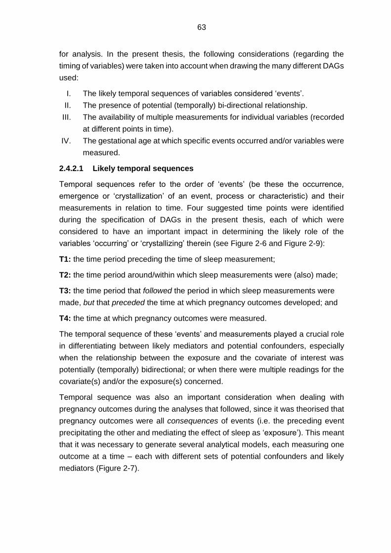
63
for analysis. In the present thesis, the following considerations (regarding the
timing of variables) were taken into account when drawing the many different DAGs
used:
I. The likely temporal sequences of variables considered ‘events’.
II. The presence of potential (temporally) bi-directional relationship.
III. The availability of multiple measurements for individual variables (recorded
at different points in time).
IV. The gestational age at which specific events occurred and/or variables were
measured.
2.4.2.1 Likely temporal sequences
Temporal sequences refer to the order of ‘events’ (be these the occurrence,
emergence or ‘crystallization’ of an event, process or characteristic) and their
measurements in relation to time. Four suggested time points were identified
during the specification of DAGs in the present thesis, each of which were
considered to have an important impact in determining the likely role of the
variables ‘occurring’ or ‘crystallizing’ therein (see Figure 2-6 and Figure 2-9):
T1: the time period preceding the time of sleep measurement;
T2: the time period around/within which sleep measurements were (also) made;
T3: the time period that followed the period in which sleep measurements were
made, but that preceded the time at which pregnancy outcomes developed; and
T4: the time at which pregnancy outcomes were measured.
The temporal sequence of these ‘events’ and measurements played a crucial role
in differentiating between likely mediators and potential confounders, especially
when the relationship between the exposure and the covariate of interest was
potentially (temporally) bidirectional; or when there were multiple readings for the
covariate(s) and/or the exposure(s) concerned.
Temporal sequence was also an important consideration when dealing with
pregnancy outcomes during the analyses that followed, since it was theorised that
pregnancy outcomes were all consequences of events (i.e. the preceding event
precipitating the other and mediating the effect of sleep as ‘exposure’). This meant
that it was necessary to generate several analytical models, each measuring one
outcome at a time – each with different sets of potential confounders and likely
mediators (Figure 2-7).

64
Figure 2-7 Directed cyclic graph arranged in a temporal sequence in which the possible causal relationships between sleep, pregnancy outcomes, and other measured covariates) is dependent upon where in the sequence these ‘occurred’ and/or ‘crystallized’.
2.4.2.2 Bidirectional relationships
Within the temporal framework used to specify DAGs in the present thesis,
bidirectional relationships are likely to exist whenever variables occurred (or
crystallized) at exactly the same time. Although these might appear to require
bidirectional arcs/arrows (something that is explicitly not permitted directed acyclic
graphs), they can be operationalised within DAGs by assuming that the two (or
more) variables involved are both causally linked by at least one preceding variable
– such that if no such variable exists, a new (hitherto unknown) ‘latent’ variable can
be specified acting as the common cause of the two (or more) variables concerned.
An example of these sorts of ‘simultaneously crystallizing’ variables in the present
thesis might be sleep and behavioural risks, each of which were assessed at a
single point in time, and both of which seem (very) likely to have caused one
another (on the basis of temporal logic and theoretical understanding of how these
variables functionally relate to one another; see Figure 2-8). In the present thesis,
whenever such measurements of simultaneously crystallising variables preceded
the measurement of others, the former were considered likely causes of the latter.
Often this approach can make it challenging to be sure which variable preceded
another, particularly in datasets collected cross-sectionally (such as the data
available for each wave of the UKHLS. Under these circumstances, when the time
of ‘occurrence’ or ‘crystallization’ measurement was uncertain or unknown, the
covariates concerned were not included in the analytical statistical models to avoid

65
the risk of adjusting for covariates acting as mediators and thereby generating an
estimation bias – in effect, the risk of under adjustment for confounding was
deemed less worrisome (given other confounders had been adjusted for) than the
risk of inappropriate adjustment for mediators.
Figure 2-8 DAG displaying the hypothesised temporal sequence of variables available for use in the UKHLS (above) and Scott/Ciantar study (below) datasets.
2.4.2.3 Use of multiple readings for individual variables
For some of the variables of interest that were available in the UKHLS and
Scott/Ciantar study datasets (i.e. variables relating to sleep, potential confounders,
likely mediators and/or pregnancy outcomes), measures were available at more
than one-time point. To address how best to use such data, the first step was to
identify the time point at which sleep had been measured and the time point at
which when the pregnancy outcomes occurred. Once these time points had been
set, it was possible to select only those measurements of covariates acting as
confounders one of whose (multiple) readings had preceded the measurement of
sleep (and could therefore be safely assumed to represent a potential confounder).
Meanwhile, for covariates with multiple readings that were believed to act as likely

66
mediators, the only consideration was whether one of the multiple measurements
available might actually precede the measurement of sleep and might therefore be
used as a potential confounder rather than a likely mediator. The frequency of
variables with multiple readings was most common in the Scott/Ciantar study
dataset, where the clinical context facilitated (and, on occasion, required) the
repeated measurement of some key variables. One such variable was BMI, this
being measured at the very first antennal visit, at the first diabetic clinic visit and
additionally prior to delivery. In order to adjust for BMI as a confounder, the BMI
measured at the first antenatal clinic would have had to have been considered as
‘crystallizing’ prior to the measurement of sleep, which it was – hence, in this
instance, it was this measurement of BMI that was included in the covariate
adjustment sets used.
Figure 2-9 A DAG summarising the treatment of multiple readings for confounders, mediators, exposures and outcomes indicating how the temporal sequence of these measurements influences the choice of reading to include in the analytical models based thereon.
2.4.2.4 Gestational age
The gestational age at which sleep was measured had substantial importance to
the analyses presented in Chapters 5 and 6 of the present thesis (Figure 2-10), not
least because it determined the temporal sequences of variables before and after
the sleep measurements were made, and therefore which covariates would act as
a likely mediators or potential confounders. If, for example, sleep was measured in
the first trimester, then the vast majority of pregnancy-related variables that

67
followed thereafter (e.g. GDM or PIH) could only act as mediators or outcomes. In
contrast, where sleep was measured in late pregnancy, then all of the preceding
pregnancy-related variables would act as potential confounders (e.g. GDM, PIH or
SGA). The principal difficulty encountered (particularly with regard to specifying the
DAG) was therefore where sleep was measured in the late second or early third
trimester, since it was then often challenging to determine which of the pregnancy-
related variables were measures of phenomena that had occurred/crystallized prior
to or after the measurement of sleep. The approach adopted under these
circumstances was that, whenever the precise timing of the ‘late pregnancy’ events
were unknown in relation to the measurement of sleep, the former were assumed
to act as likely mediators and were therefore excluded from the covariate
adjustment sets used (a consequence of which might be that the estimates
generated by these multivariable, adjusted models might have suffered from
unadjusted confounding even from confounders for which measurements were
available).
In the UKHLS, there were insufficient numbers of participants with data on
gestational age at the point of sleep measurement, and for this reason it was
unclear when the sleep of most participants had actually been measured. For this
reason, it was decided that none of the variables relating to pregnancy-relevant
phenomena (such as GDM) should be included in the covariate adjustment sets
used (again, eliminating the risk of inappropriate mediator adjustment whilst
accepting the risk of incomplete adjustment for potential confounding).

68
Figure 2-10 Three alternative DAGs intended to illustrate the changes in casual pathways observed amongst the study’s variables where the measurement of sleep occurred in each of the three trimesters of pregnancy.
2.4.3 Application of DAGs
During the critical appraisal of primary studies identified during the systematic
review and meta-analyses presented in Chapter 3 of the present thesis, each of
the primary studies examined was individually assessed with regard to the choice
of covariates included in any adjustment sets used. This involved compiling a
complete list of all covariates that had been included in adjustment sets by any of
these studies, and using these to construct a theoretical causal path diagram (in
the form of a DAG) using known (or hypothesised) temporal relationships between
the covariates, exposure(s) and outcome(s), from which it was then possible to
identify any covariates likely to have acted as potential confounders and any that
were likely to have been mediators. In addition, the very same temporal rules
adopted when drawing DAGs to inform the design of statistical models used in later
chapters (i.e. Chapter 5 &6) were also used to carefully consider whether
inappropriate adjustment might have occurred in any of the models reported by the
primary studies reviewed. This involved only including estimates derived from
models adjusting for no possible mediators in the synthesis of evidence and/or
meta-analyses presented in this chapter.

69
In the course of the two observational analytical studies (in Chapters 5 and 6; as
well as in the latter part of Chapter 4) a wide range of measured (and therefore
‘manifest) covariates were identified as potential confounders. However, in the
UKHLS dataset, there were limited data on the health of study participants (such
as pre-pregnancy BMI) or on the gestational age at questionnaire completion (i.e.
when sleep, and other covariates, were actually measured). In contrast, in the
Scott/Ciantar study’s dataset, there were limited data on some potentially important
sociodemographic characteristics (such as education and employment), though
substantial data on a wide range of health and clinical factors. Both pregnancy
studies nonetheless had (as already described, see Table 2-2) only modest
numbers of participants and this meant it was likely that (at least from a parametric
point of view) the scope for including large numbers of covariates in the adjustment
sets used was likely to be limited. To address the latter concern, the covariates
considered potential confounders were, wherever possible, recoded as binary
variables to reduce the number of categories involved (and the number of degrees
of freedom required), thereby permitting the inclusion of as many covariates (i.e.
those acting as potential confounders) as possible.
2.4.4 Limitations of the ‘DAG approach’
Although DAGs are considered a very useful tool when modelling multivariable
systems, they nonetheless retain a number of substantive limitations, especially
when the relation between the exposure and the outcome is complicated (as is the
case for the relation between sleep and pregnancy outcomes; Shrier and Platt,
2008).
First of all, DAGs only permit unidirectional relationships between variables – an
assumption that is difficult to justify in real life since many variables are ‘time-
variant’ and can affect one another in a sequence that would be evident were a
sequence of measurements on each to be available (Textor et al, 2011). However,
this limitation was mitigated by applying the temporal sequences of measured
events as hypothesised in terms of the likely consequences of any tendency for
bidirectional relationships between two variables to move, primarily, in one
direction over time.
Furthermore, DAGs cannot improve the inherent uncertainty in casual inference
relating to a study’s inherent design and data measurement limitations (such as
selection bias or measurement error, respectively; Shrier and Platt, 2008,
Greenland and Morgenstern,1999) 2001). Likewise, DAGs cannot help identifying
the reference point of each included covariate that is necessary/optimal for
optimally addressing any effect of that covariate on the casual relation between
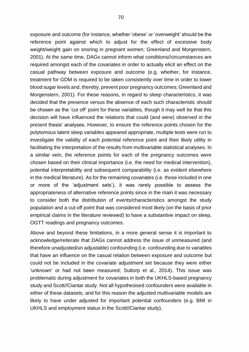
70
exposure and outcome (for instance, whether ‘obese’ or ‘overweight’ should be the
reference point against which to adjust for the effect of excessive body
weight/weight gain on snoring in pregnant women; Greenland and Morgenstern,
2001). At the same time, DAGs cannot inform what conditions//circumstances are
required amongst each of the covariates in order to actually elicit an effect on the
casual pathway between exposure and outcome (e.g. whether, for instance,
treatment for GDM is required to be taken consistently over time in order to lower
blood sugar levels and, thereby, prevent poor pregnancy outcomes; Greenland and
Morgenstern, 2001). For these reasons, in regard to sleep characteristics, it was
decided that the presence versus the absence of each such characteristic should
be chosen as the ‘cut off’ point for these variables, though it may well be that this
decision will have influenced the relations that could (and were) observed in the
present thesis’ analyses. However, to ensure the reference points chosen for the
polytomous latent sleep variables appeared appropriate, multiple tests were run to
investigate the validity of each potential reference point and their likely utility in
facilitating the interpretation of the results from multivariable statistical analyses. In
a similar vein, the reference points for each of the pregnancy outcomes were
chosen based on their clinical importance (i.e. the need for medical intervention),
potential interpretability and subsequent comparability (i.e. as evident elsewhere
in the medical literature). As for the remaining covariates (i.e. those included in one
or more of the ‘adjustment sets’), it was rarely possible to assess the
appropriateness of alternative reference points since in the main it was necessary
to consider both the distribution of events/characteristics amongst the study
population and a cut-off point that was considered most likely (on the basis of prior
empirical claims in the literature reviewed) to have a substantive impact on sleep,
OGTT readings and pregnancy outcomes.
Above and beyond these limitations, in a more general sense it is important to
acknowledge/reiterate that DAGs cannot address the issue of unmeasured (and
therefore unadjusted/un adjustable) confounding (i.e. confounding due to variables
that have an influence on the casual relation between exposure and outcome but
could not be included in the covariate adjustment set because they were either
‘unknown’ or had not been measured; Suttorp et al., 2014). This issue was
problematic during adjustment for covariates in both the UKHLS-based pregnancy
study and Scott//Ciantar study. Not all hypothesised confounders were available in
either of these datasets, and for this reason the adjusted multivariable models are
likely to have under adjusted for important potential confounders (e.g. BMI in
UKHLS and employment status in the Scott//Ciantar study).

71
Finally, using DAGs cannot deal with the risk of harmful (inappropriate) adjustment
where sample stratification occurred prior to analysis (Suttorp et al., 2014,
Greenland et al.,1999). This effect can occur when the stratification applied drew
on an event/phenomenon that occurred between the time sleep was measured and
the time that the pregnancy outcomes developed – such that the
events/phenomena concerned either mediated the effect of sleep on pregnancy
outcomes (i.e. acted as likely mediators) or were influenced by both sleep and
pregnancy outcomes (i.e. acted as a ‘collider’; Cole et al., 2009). In such
circumstances, although the hypothesised DAG will be correct, the estimation of
casual inference will be biased as a direct result of the faulty stratification (Suttorp
et al., 2014, Cole et al., 2009). While, in the present thesis, stratification for
adjustment was avoided, , it appeared to have been commonly used in many of
the studies identified in the literature, and this is likely to limit the validity and
subsequent analytical utility of the estimates produced by these studies – an issue
that required careful assessment when evaluating the quality of study results over
and above issues of (in)appropriate adjustment.
In summary, then, each of the following limitations cannot be addressed (or
improved upon) by using DAGs, and remain a key challenge to unbiased casual
inference – contributing to residual uncertainty as to whether the estimates
generated are accurate/useful irrespective of DAG-assisted assessments of the
appropriateness of adjustment:
I. limitations in study design and data quality;
II. ensuring the required circumstances/conditions are met by each of the
covariates (to reflect their optimal effects on the casual pathway);
III. the presence of unadjusted confounding; and
IV. the faulty stratification of data.
2.5 Data analysis
2.5.1 Logistic regression analysis
Multivariable logistic regression analyses, with covariate adjustment sets informed
by theoretical causal path diagrams (in the form of a DAG), specified a priori, was
the principal statistical technique used by the two de novo observational analytical
studies conducted for the present thesis (i.e. those analyses presented in Chapters
5 and 6). Logistic regression is a statistical technique that assesses the association
between one or more independent variables and a dependent binary variable.
Unlike t-tests, chi-square tests and correlation analyses, logistic regression permits
the inclusion of additional variables (i.e. covariates) so that the analyses are able

72
to adjust for those covariates acting as confounders (Peng et al., 2002). This
technique was deemed a suitable choice for the analysis of data in Chapters 5 and
6 of the present thesis since the poor pregnancy outcomes were amenable to
(re)coding as either “absent” or “present.” Likewise, the presence of many potential
confounders in any such analyses of the association between sleep and pregnancy
outcomes necessitated careful covariate adjustment – another key issue in the
choice of logistic regression as the principal analytical technique used in the
present thesis.
For similar reasons, multivariable logistic regression analysis was also used in
analyses of UKHLS data to assess the criterion-based validity of latent sleep
patterns identified using latent class analysis (LCA, see Section 2.5.2, page 79).
This involved examining the associations between a range of sociodemographic
and health characteristics considered likely determinants/predictors of latent sleep
patterns. However, the estimation methods used in these analyses (i.e. in Chapters
4, 5 and 6) varied somewhat depending upon the sample size available and the
distribution of the exposure and outcome variables.
2.5.1.1 Estimation method
In the analysis of latent sleep patterns using UKHLS data (Chapter 4), the
estimation method used for its logistic regression analyses was the maximum
likelihood estimation – the standard estimation method used within logistic
regression and the default estimation available within the STATA statistical
analysis software used. By contrast, when analysing the association between sleep
and pregnancy outcomes using data from the UKHLS and Scott/Ciantar studies
(i.e. Chapters 5 and 6, respectively), the estimation method used was the penalised
maximum likelihood estimation (Firth, 1993). The reason why this alternative
estimation method was chosen was because of the small sample sizes available
for analysis in each of these analyses, and the limited number of participants in
each who had poor pregnancy outcomes.
Logistic regression analyses using the maximum likelihood estimation method is
limited for small sample sizes (< 200) (Hirji et al., 1987, Firth, 1993, Mehta and
Patel, 1995, King and Zeng, 2001) because it underestimates the probability of
rare events (King and Zeng, 2001), leading to an inflated estimate with a larger
standard error. An alternative to maximum likelihood estimation is the exact logistic
regression (Hirji et al., 1987, Mehta and Patel, 1995), which works with both
unbalanced and small sample sizes (< 200). However, this method has a number
of additional limitations: first, the number of covariates permitted in the model is (or
should be) limited, and each must be dichotomous; and second, substantial

73
computing power is required to generate the estimation. In the present thesis, the
estimation method used was therefore exact logistic regression – chosen because
the sample size available was less than n=200 and there were relatively few
covariates. However, an initial trial of using this method failed due to a hardware
memory shortage. Instead, the present thesis considered using a new estimation
method, proposed by King and Zeng (2001) – a method that is mainly used with
large sample sizes and rare events, and seems to over-correct the maximum
likelihood estimation when applied to small sample sizes (such as those used in
the present study). As a result, the present thesis used a method first described by
Firth (1993), the penalised maximum likelihood estimation, which prevents
estimation bias and works well with small sample sizes; allowing for the use of
many covariates, even those that are not dichotomous; and without the need for
excessive computer memory. The STATA software provides this estimation
method as the ‘Firthlogit’ command, and this was the command used to enact this
estimation method in Chapters 5 and 6 of the present thesis.
2.5.1.2 Estimated statistical power of the regression analyses
The achieved statistical power of the regression analyses included in Chapters 4,
5 and 6 of the present thesis was calculated post hoc, after the sample size and
odds ratio-based estimates that had been achieved. As there were a range of
different values for the odds ratios generated by Chapter 4-6’s logistic regression
analyses, the estimation of statistical power was carried out using a range of
different odds ratio values (see Table 2-2). The level of alpha selected was 0.05
and the sample sizes available were n=294 for the analysis of sleep and pregnancy
outcomes using UKHLS data, and n=108 using data from the Scott/Ciantar study;
while the probability of a positive outcome when the exposure was present was
assumed to be 0.5. Based on these criteria, in order to be able to detect a 10%
change in risk with a power of 0.8, the sample size required would have had to
have been ~n=3,500 – 15-30 times larger than that actually available in the
analyses summarised in Chapters 5 and 6; making both sets of analyses
extensively underpowered (and therefore at risk of type I and II error, and of a
substantial loss of precision). The software used for these estimations was
‘Gpower’ (Faul et al., 2009), which was based on research undertaken by
Demidenko (2006).
While these power calculations identify a sobering limitation of the analyses
conducted within Chapters 5 and 6 of the present thesis, they are also important
for screening the literature included in the systematic review and meta-analyses
presented in Chapter 3. This is because a priori knowledge of the likely statistical

74
power required, and the sample sizes needed to achieve this, can help to reduce
the possibility of type I and type II errors. However, in Chapter 3, the post hoc
power estimation analyses conducted for each of the studies included in the review
were conducted on the basis of assumptions that were similar to those applied to
the two empirical datasets examined de novo in the present thesis.

75
Table 2-2 The statistical power achieved by regression analyses across a range of odds ratio values with alpha set at 0.05; focussing specifically on the final sample size available for analysis using data from the UKHLS (n=294) and the Scott/Ciantar study (n=108).1
Odds ratios
0.3 0.4 0.5 0.6 0.7 0.8 0.9 1.1 1.2 1.3 1.4 1.5 1.6 1.7 1.8 1.9 2.00
UKHLS
(n=294)
1.00 0.97 0.78 0.45 0.18 0.16 0.34 0.55 0.74 0.87 0.93 0.98 0.99 1.00
Scott/Ciantar
(n=108)
1.00 0.98 0.87 0.66 0.42 0.23 0.11 0.11 0.18 0.28 0.39 0.50 0.60 0.70 0.76 0.83 0.87
1 Bold text indicates the acceptable level of power (i.e. 0.8 and above).

76
2.5.1.3 Multiple testing
Multiple testing (or examining multiple hypothesis using a single data set) can be
problematic since it can increase the possibility of type I error/false positive results
(i.e. in this instance suggesting an association between sleep and poor pregnancy
outcomes exists when, in fact, the association is absent). To address this it is
considered necessary to adjust the alpha level so that this is then appropriate for the
total number of tested hypotheses (Benjamini and Hochberg, 1995). To illustrate this
further, at a 5% level of significance, were a single test to be conducted and the null
hypothesis were true, there would be a 5% chance of falsely rejecting the null
hypothesis. However, were 20 tests to be conducted simultaneously, using exactly the
same data and the same level of significance there would be 64% chance of falsely
rejecting one of the null hypotheses even if all of the null hypotheses tested were
actually true (Bender and Lange, 2001). The chance of rejecting the null hypothesis
as a result of a ‘statistically significant’ result therefore tends to increase as the number
of tested hypotheses (i.e. regression models) increases. For this reason, the alpha
level set should be adjusted according to the number of hypotheses tested, thereby
reducing the possibility of detecting a false positive association. Such adjustments
(generally labelled ‘corrections’) can be achieved done using a range of different
techniques such as the Bonferroni method, in which the alpha level is simply dividing
by the number of tested hypotheses (Bonferroni, 1936).
Multiple testing and the elevated risk of a type I error associated therewith, was
actually a more problematic issue for the systematic review and meta-analyses
conducted in Chapter 3 of the present thesis. This is because many authors commonly
overlook the fact that they have run multiple, simultaneous tests and publish the
results of these as if they were independent. In the empirical analyses undertaken for
this thesis (i.e. in Chapters 4-6), the presence of multiple testing was carefully
examined and, where evident, the alpha level was corrected using the Bonferroni
method. Whilst this approach may be of particular interest to those analysts focusing
on the statistical significance and precision of the estimates generated in these
analyses, the main focus of the present thesis was on the clinical significance (i.e. the
direction and strength) of the estimates and only secondarily on the levels of precision
(i.e. statistical significance) achieved. For this reason, odds ratios with higher
magnitudes (with or without narrower confident intervals) formed the principal basis
for assessing the clinical significance of these analyses’ findings, and such findings
formed the basis upon which theoretical speculation and interpretation was then

77
undertaken, for the most part regardless of the statistical p-value these estimates
attained.
For a number of related reasons, the p-values calculated by analyses in the present
thesis were felt to be potentially misleading:
I. First, these p-values relate to an examination of the null hypothesis rather than
a chosen alternative hypothesis, since it remains uncertain whether the
alternative hypothesis chosen or another (alternative) hypothesis are likely to
be be true (Goodman, 1999)
II. Second, the presence of multiple testing is likely to have elevated the risk of
rejecting the null hypothesis even though the null hypothesis might actually be
true (Bonferroni, 1936).
III. Third, the small sample sizes available for the de novo analyses are likely to
have increased the risk of accepting the null hypothesis even though/when the
null hypothesis might actually be false (Akobeng, 2016)
For these reasons, it was considered better (if not best) practice not to report p-values
for the de novo analyses presented in the present thesis. Nonetheless, although p-
values were not reported in these results, estimates with confidence intervals
indicating these exceeded a null based on ‘no effect’ (i.e. at a p-value <0.05) were
highlighted in bold text in the Tables that follow, in order to draw the attention of the
reader to these while signaling that the ‘significant’ p-values concerned are at
increased risk of occurring simply by chance (especially where these analyses
involved multiple testing) and indicating that careful circumspection was warranted
when interpreting these results. Thus, instead of reporting the precise p-value, and
commenting on its relevance as a potential indicator of certainty (and/or precision),
95% CIs were used throughout the present thesis to offer a clearer indication of the
precision achieved (even though it was expected that the level of precision achieved
would, for the most part, be modest as a result of the small sample size of participants,
and the impact of this on the limited power of these analyses; Akobeng, 2016, Button,
2013, Poole, 2001)
2.5.1.4 Identification and adjustment for potential confounders
The majority of confounders identified in the analyses presented in this thesis were
adjusted for by including these in the covariate adjustments sets of the multivariable
regression models used. This approach (adjustment) was chosen in preference to
alternatives (particularly stratification) due to the small numbers of participants

78
available for the analysis of sleep and pregnancy outcomes (in Chapters 5 and 6), the
presence of (at least some) continuous confounders, and the comparatively large
number of potential confounders – since stratification, for example, would have
substantially reduced the statistical power of these tests (Weinberg, 1993).
However, it was important to correctly identify potential confounders, to distinguish
these from likely mediators, and not to under-adjust for any available/measured (so-
called ‘manifest’) confounders, since inappropriate and under-adjustment can both
lead to biased causal inference (Textor et al., 2017). While under-adjustment
(including an insufficient number of confounders), might lead to either an
underestimation or an overestimation of the causal relationship, the inclusion of more
covariates in the adjustment sets used, particularly when the number of discrete
observations (such as study participants) is low, can decrease the parametric stability
of the statistical model used (Vittinghoff and McCulloch, 2006) or decrease its power
(Textor and Li´skiewicz, 2017). In terms of the latter, some authors have suggested
that a useful rule of thumb is that the number of covariates included in multivariable
adjustment sets should not exceed one for every 10 to 20 observations/participants
(Concato et al., 1995, Peduzzi et al., 1996, Vittinghoff and McCulloch, 2006). Yet this
concern is largely secondary to correctly identifying potential confounders and
including these (and not mediators), in the adjustment sets used (since adjusting for
mediators might can cause estimation bias; VanderWeele, 2009).
Variables related to each of the exposures and outcomes were identified within the
UKHLS and Scott/Ciantar studies datasets, and the choice of which were
subsequently used was based on their availability, likely/actual levels of
acuity/missingness, clinical expertise and empirical evidence from the literature. The
variables selected in this fashion were then mapped onto a directed acyclic graph
(DAG), where all of the potential causal relationships between the variables could be
drawn. Using a DAG in this way was felt to be an important step, since a substantial
number of potential variables were related to both the exposure (sleep) and the
outcomes (pregnancy outcomes), especially in the large UKHLS dataset. However,
given the limited knowledge/certainty regarding the temporal sequences of (and
thereby potential causal relationships between) events/variables in the UKHLS
dataset, together with the limited number of pregnant participants in both datasets, it
was necessary to limit the number of variables/covariates included in the analyses’
covariate adjustment sets, and include only those considered definitive confounders,
and those considered likely to exert string (causal) effects on both exposure and
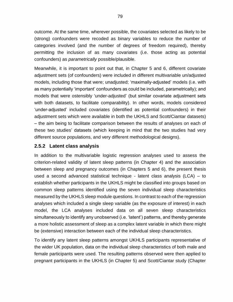
79
outcome. At the same time, wherever possible, the covariates selected as likely to be
(strong) confounders were recoded as binary variables to reduce the number of
categories involved (and the number of degrees of freedom required), thereby
permitting the inclusion of as many covariates (i.e. those acting as potential
confounders) as parametrically possible/plausible.
Meanwhile, it is important to point out that, in Chapter 5 and 6, different covariate
adjustment sets (of confounders) were included in different multivariable un/adjusted
models, including those that were; unadjusted; ‘maximally-adjusted’ models (i.e. with
as many potentially ‘important’ confounders as could be included, parametrically); and
models that were ostensibly ‘under-adjusted’ (but similar covariate adjustment sets
with both datasets, to facilitate comparability). In other words, models considered
‘under-adjusted’ included covariates (identified as potential confounders) in their
adjustment sets which were available in both the UKHLS and Scott/Ciantar datasets)
– the aim being to facilitate comparison between the results of analyses on each of
these two studies’ datasets (which keeping in mind that the two studies had very
different source populations, and very different methodological designs).
2.5.2 Latent class analysis
In addition to the multivariable logistic regression analyses used to assess the
criterion-related validity of latent sleep patterns (in Chapter 4) and the association
between sleep and pregnancy outcomes (in Chapters 5 and 6), the present thesis
used a second advanced statistical technique - latent class analysis (LCA) – to
establish whether participants in the UKHLS might be classified into groups based on
common sleep patterns identified using the seven individual sleep characteristics
measured by the UKHLS sleep module questions. In contrast to each of the regression
analyses which included a single sleep variable (as the exposure of interest) in each
model, the LCA analyses included data on all seven sleep characteristics
simultaneously to identify any unobserved (i.e. ‘latent’) patterns, and thereby generate
a more holistic assessment of sleep as a complex latent variable in which there might
be (extensive) interaction between each of the individual sleep characteristics.
To identify any latent sleep patterns amongst UKHLS participants representative of
the wider UK population, data on the individual sleep characteristics of both male and
female participants were used. The resulting patterns observed were then applied to
pregnant participants in the UKHLS (in Chapter 5) and Scott/Ciantar study (Chapter

80
6), amongst whom the relationship between these latent sleep patterns and each of
the pregnancy outcomes were then investigated.
2.5.2.1 LCA estimation method
Latent Gold 4.5 software (Statistical Innovations Inc., 2009) was used to conduct the
LCA analyses. This software calculates the posterior probability of each participant’s
‘membership’ within each latent class, and these probabilities can then be used to
assign that class to the individual concerned which achieves the highest probability
(using the maximum likelihood as the key estimation method; Vermunt and Magidson,
2005).
2.5.2.2 Identifying the best-fitting latent model
At first, exploratory LCA analyses were conducted to generate models with a wide
range of (sleep) clusters; after which two key information criteria (i.e. the Bayesian
information criterion [BIC] and the Akaike information criterion [AIC]), together with
two entropy statistics (i.e. R2 and model estimation error), were used to compare
different models with varying numbers of clusters. In each case, the lower the
information criteria and the higher R2 the more robust the model was assumed to be,
after ‘penalising’ the statistics by the number of variables included therein (as
recommended by Vermunt and Magidson, 2005). However, although these four
statistical parameters were used to assist in the identification of the ‘best-fitting’
models, two further ‘stability’ sub-analyses were also conducted to verify the
consistency of cluster classifications- the first over time and the second within the
population examined. These stability sub-studies were important to ensure that the
UKHLS sleep module data were capable of detecting/generating similar clusters that
were stable over time and place (see Section 2.5.2.3).
2.5.2.3 Stability of the chosen latent class model
The two ‘stability’ sub-studies assessed whether similar clusters were produced using
LCA applied to data collected (by the UKHLS) at different points in time or in different
(sub)populations; though this assessment did not evaluate whether the participants
allocated to each sleep cluster remained within these over time (i.e. what might be
termed ‘membership stability’ rather than ‘cluster classificatory’ stability). Each of
these ‘stability’ sub-studies were conducted as follows:

81
1) Stability within sub-samples
This first stability study compared the classification of sleep clusters between:
I. a sub-sample of participants who participated in Wave 1 only;
II. a sub-sample of participants who participated in Wave 4 only; and
III. all participants who participated either in Wave 1 and/or Wave 4.
This study assessed whether the sleep clusters that were identified among all
participants (i.e. sample III) were the largest-size sleep clusters identified in the two
sub-samples (i.e. samples I and II).
2) Stability of sleep clusters over time
This sub-study examined exactly the same UKHLS participants over two discrete time
points (i.e. using data they provided at Wave 1 and again at Wave 4). The aim was to
assess whether the same (number and classification of) sleep clusters would be
generated using LCA on data from the same participants (regardless of any changes
in the membership of individuals to any given sleep cluster) over time.
2.5.2.4 LCA power assessment
During the literature searches conducted in the course of the present thesis, no
appropriate “rule of thumb” emerged for conducting LCA power estimation, although
several authors have made related recommendations. One of these suggested that
there should, ideally, be 10-15 observations per parameter, which implies that in the
present thesis’ LCA analyses, at least 210 to 315 participants would be required for
the 21 discrete sleep parameters assessed using the UKHLS sleep module (i.e. those
that were used in generating the latent sleep models; Comrey and Lee, 1992). An
alternative recommendation was that no latent class analysis should be conducted on
samples smaller than 100 participants (Gorsuch,1983, Kline,1979); while a sample of
1000 participants was felt sufficient to generate ‘excellent’ analytical power (Comrey
and Lee, 1992). Likewise, a sample of 200-250 was felt to afford ‘fair’ estimation power
(Comrey and Lee, 1992, Cattell, 1978, Guilford, 1954). Meanwhile, on the basis of
several Monto Carlo studies simulations, some authors suggest that a larger sample
size can be required when the aim of the LCA analyses is to detect small-sized
clusters or a larger number of clusters, and when larger numbers of indicators with
limited variability across the sample are used (Dziak et al., 2014, Tein et al., 2013,
Nylund et al., 2007). As such, all of these (somewhat eclectic) recommendations
suggest that the analyses undertaken for this part of the present thesis had ample

82
power, since the UKHLS dataset drew on a population-based study with a very large
sample size (>50,000 households) – a sample that was more than large and variable
enough to ensure a sufficient level of power to estimate cluster-based classifications
using LCA analysis.
2.5.3 The treatment of missing data
Prior to the exclusion of missing data, these data were examined for the “missing at
random” assumption. Missing completely at random means that the missing data do
not systematically differ from the observed data, since the cause of missingness is
unrelated to the data (van Buuren, 2012). However, missing completely at random is
extremely difficult to assess, thus a broader assumption ‒ missing at random ‒ was
examined instead (Van Buuren, 2012, Cattle et al., 2011). The missing at random
assumption means that any possible systematic difference between the missing data
and the observed data could be explained by differences in the characteristics of the
observed data (Van Buuren, 2012, Sterne at al., 2009). For example, missing blood
pressure measurements might be lower than reported blood pressure measurements
but only because women in their very early pregnancy may be more likely to have
missing blood pressure measurements (Sterne at al., 2009). It was important to
assess the “missing not at random” assumption, as this would bias the estimates
generated by analyses in which variables and/or participants were excluded on the
basis of missing data (Allison, 2002). Missing not at random simply means that the
missing data are systematically different from the observed data for reasons that can
not be explained by the observed characteristics of the data (Van Buuren, 2012, Cattle
et al., 2011). For instance, participants with low socioeconomic status might avoid
reporting their income because of their hidden worries (Cattle et al., 2011) or pregnant
women with GHTN might not attend their antenatal care clinic because they have
headache (Sterne et al., 2009).
In the present thesis, it was originally considered worthwhile using multiple imputation
to deal with missing data, since multiple imputation is considered superior to all other
method for treating missing data (Van Buuren, 2012, Rubin, 2004). However, rather
than imputing values for missing data, the variables and/or participants with any
missing data were instead simply excluded (i.e.listwise deletion) – a technique that
deals with missingness but only at the risk of creating biased analytical samples, and
decreasing the statistical power of the sample available for analysis. However, this
approach (variable or participant deletion) may still be superior to most other
imputation techniques (particularly simple ones), as it is capable of generating a

83
sample on which an unbiased estimate can be calculated provided the “missing at
random” assumption can be upheld (Allison, 2002). That said, multiple imputation (a
complex, multistage imputation method, recommended by many authors including
Rubin, 1996), would not have biased the estimate, and would have improved the
standard error of the estimate and preserved the power of the analyses (Van Buuren,
2012, Rubin, 2004). However, Sterne et al. (2009) have pointed out that a lack of
experience in multiple imputation can often generate misleading results and incorrect
conclusions (Sterne et al., 2009). In the event, multiple imputations could not be used
to address problems with missing data in the UKHLS dataset due to computational
limitations, many of which resulted from the sheer size and complexity of the UKHLS
dataset (i.e. a very large dataset containing some variables with a very large number
of response categories). On the other hand, the power of the analyses in the
Scott/Ciantar study would have remained severely underpowered even were multiple
imputation to have been applied. Likewise, the number of auxiliary variables (i.e.
variables which are included in the imputation model but not in the main regression
model of the analysis; Thoemmes and Rose, 2014, Little and Rubin, 2002) required
to impute values for missing sleep and medical variables with sufficient certainty were
severely limited by the small number of such variables with complete data (i.e. n=108)
– a substantive problem given a minimum of 10 participants per variable were required
for inclusion in the imputation model and given that the number of auxiliary variables
included should not be more than one third of the cases with complete data (i.e. all
participants excluding those with missing data, Hardt et al., 2012).
Finally, some of the variables that would have been important to include in any
imputation models (particularly those required to impute missing sleep and/or
pregnancy outcome data) were unavailable within either of the two datasets: in the
UKHLS there was insufficient information on pregnancy-related variables (e.g.
gestational age and BMI) to use as predictors in the imputation model; whilst in the
Scott/Ciantar study there were insufficient sociodemographic and psychological
measures to include in the imputation model for missing sleep variables. Multiple
imputation would nonetheless remain an aspiration for future research in this field (see
Discussion, Chapter 7), not least because most of the studies reviewed in the present
thesis appeared to have avoided using multiple imputation and instead chose to delete
cases with (any, relevant) missing data. That said, the best solution to the challenge
of missing data is to avoid this during data collection, or by including more cases and
variables so that these are available to inform subsequent multiple imputation (e.g.

84
larger studies with data on a greater variety of sociodemographic and medical-related
variables, and with better data quality/completeness).
2.6 Conclusion
The present chapter aimed to briefly describe the rationale behind the samples, data
and analytical techniques used in the analytical chapters that follow. These involved
two principal, advanced statistical techniques (latent class analysis, or LCA; and
multivariable logistic regression) the latter informed by recent advances in causal
inference techniques (particularly the use of directed acyclic graphs, or DAGs, to
identify suitable covariate adjustment sets for inclusion in multivariable statistical
models). Some of these methods were used in the systematic review and meta-
analyses undertaken in Chapter 3, which helped to strengthen the choice of analytical
methods in the present thesis. Further detail on many of the methodological decisions
made when planning and conducting the present thesis can be found in the Appendix
– detail collated therein to ensure that the remainder of the thesis was clear and easy
to read and assimilate.

85
Chapter 3 Systematic review and meta-analysis
3.1 Introduction
As described earlier, in the introductory chapter to the present thesis, there
appears to be a reasonable amount of evidence of various associations across a
range of sleep characteristics and pregnancy outcomes in the published scientific
literature; much of this evidence suggesting that unfavourable sleep is associated
with an increased risk of poor pregnancy outcomes (Ding et al., 2014).
Unfavourable sleep (including shortened sleep duration and disturbed sleep) are
reportedly common during pregnancy, these phenomena often being attributed to
the effects of the many physiological, anatomical and psychological changes that
occur during each successive trimester of pregnancy. Indeed, since there are
different bio-social phenomena involved during each trimester of pregnancy these
also appear to display differing frequencies of unfavourable sleep events.
Meanwhile, some poor pregnancy outcomes (such as low birth weight and preterm
delivery) can be determined early in pregnancy by genetic, phenotypic or
environmental factors including maternal health, height and socioeconomic
position. Such factors may be resistant to clinical modification, whilst others
(including sleep) might be more amenable to improvement or optimisation through
educational and/or behavioural intervention. As such, the potential importance of
sleep (and other, ostensibly modifiable ‘lifestyle’ factors) warrant careful
examination; not least because of the evidence provided by previous studies which
(appears, at first sight, to) indicate an association between (less favourable) sleep
and (poor) pregnancy outcomes.
Sleep in pregnancy remains a relatively under-researched topic that faces many
unusual challenges due to the sensitive nature of pregnancy; the rapid maternal
changes and foetal development that occurs therein; the complex nature of sleep;
and much that is still unknown about the biological basis (and consequences) of
sleep. For this reason it might therefore be expected that research in this area is
somewhat limited, particularly that adopting experimental/intervention-based study
designs since these are likely to be considered high risk for mothers and their
unborn child, and therefore subject to levels of ethical scrutiny, participant
resistance and/or lack of compliance that make them very challenging to conduct.
In this chapter of the present thesis, a systematic review will be undertaken to
summarise and evaluate the research evidence available of an association

86
between sleep and pregnancy outcomes, and thereby highlight the possible gaps
(flaws and limitations) in this evidence. This is considered an important first step in
the analyses presented later in the present thesis, since it aims to avoid repetition
(except where replication might add novel insights or confirmation of existing
findings) and avoid (m)any of the flaws and errors that may have undermined the
quality of the evidence currently available.
3.2 Methods
3.2.1 Systematic review
3.2.1.1 Time scale
The systematic search undertaken for the present chapter’s review and meta-
analysis took place at the beginning of the period of Doctoral study, and the initial
search therefore focussed on publications up until January, 2014. However, to
update the results of these searches, towards the end of the period of study, the
same search was undertaken to identify any articles papers that had been
published between January 2014 (the date of the original search) and March 2017
(the date of the second search).
3.2.1.2 Search terms and engines
Dedicated search terms were used to identify articles that included a focus on sleep
and pregnancy, by applying these terms in the EMBASE and Medline databases.
These terms had been developed by NA Al Afif (a fellow doctoral student at the
University of Leeds, whose thesis examined the impact of pregnancy on sleep),
using terms collated from published systematic reviews that had used these to
review topics in which sleep and/or pregnancy had been involved. Subsequent pilot
tests using these terms found them to display high sensitivity in detecting
references to sleep in articles examining pregnancy or pregnancy-related issues
(Al Afif, 2016). To maintain the highest possible level of sensitivity, terms within
each group (i.e. with those synonyms for ‘sleep’ and for ‘pregnancy’) were linked
with “or”, while the two groups were then linked with “and”.
Group one: sleep-related terms
Central sleep apnea, sleep apnea, apnea, obstructive sleep apnea, obstructive
sleep, sleep-related breathing, insomnia, sleep*, sleep time, sleep duration, sleep
hours, time in bed, sleep quality, sleep disorder, sleep disorders, sleep disordered,
time spent asleep, time spent sleeping, time asleep, sleep length, dysomnia,
parasomnia, hypersomnia, sleep disturbance, sleeplessness, sleep efficiency,

87
sleep latency, sleep problem, sleep disturbance, sleep difficulties, nightmare, sleep
deprivation, and sleep terror
Group two: terms related to pregnancy outcomes (obstetric, perinatal, and
neonatal)
Pregnancy, pregnan*, pregnant women, pregnancy complication, pregnancy
trimester, obstetric complication, maternal, obstetric, maternal age, maternal
complication, pregnancy outcome, pregnancy in adolescence, pregnancy rate,
maternity care, paternal, antenatal, gestational outcome, and gestation.
3.2.1.3 Search inclusion criteria and screening strategies
Using the options available in each of the databases searched, the search was
limited to include only the following types of studies;
I. human studies
II. female studies
III. adult studies.
In a later step, the titles, abstracts, and full texts of the resulted studies were
screened manually; those whose content did not match the topic (sleep in
pregnancy) or the limits intended (as at I, II and III, above) were excluded using
each of the following exclusion criteria:
I. animal studies
II. studies irrelevant to sleep
III. studies relevant to sleep but not related to pregnancy
IV. studies relevant to sleep in pregnancy that did not examine the
relationship between sleep and pregnancy outcomes
V. non-primary studies such as meta-analyses, reviews, opinion/consensus
documents/pieces, and non-quantitative studies
Screening was performed twice by two independent reviewers: the candidate (AA
Alghamdi) and a Doctoral colleague (NA Al Afif. The screening results of each
reviewer were compared, and any disagreements were discussed and resolved.
3.2.2 Data extraction method
After reading the full text of each article screened for inclusion in the review, five
sets of Tables were created.
The first table summarises pertinent general information about each article,
including the author, year of publication, relevant study inclusion and exclusion
criteria, the study setting, and any reported characteristics of the population
studied.

88
The second table summarises information about the exposure examined, including
its timing, the measurement tools used, the definition thereof and/or reference point
used, and any available descriptive statistics.
The third table adopts a similar structure to the second table, but focusses on the
pregnancy outcomes examined rather than the sleep exposures of interest.
The fourth table contains information about any covariates measured in each of
the studies reviewed, including similar details to those contained in the second and
third tables.
The fifth table includes details of any regression models used by each of the
studies, including the exposure and outcome used, any covariate adjustment sets
used, a narrative regarding any justification given for the adjustment set(s) used,
and the results of these analyses expressed as logistic odds ratios (OR) with 95%
confidence intervals in parentheses.
At this stage of data extraction, any articles that had not used multivariable
regression models to analyse their data were excluded from the review – the
principal rationale for this was simply that in the absence of any adjustment for
potential confounding the results of these studies’ analyses are likely to have
suffered from confounding bias.
A directed acyclic graph (DAG) was drawn for each article to represent the
temporal sequence and potential causal relationships between each of the
measured covariates, and the exposure and outcome of interest. These, separate,
DAGs were then combined into a single DAG summarising the theoretical causal
relationships between all of the covariates (exposures and outcomes) measured
across all of the studies included. Variables for which each studies’ analyses were
judged to have adjusted included not only those included in the covariate
adjustment sets of any multivariable statistical models, but also any variable for
which the study was restricted during sampling or stratified during analysis.
3.2.3 Quality assessment of the studies
Each of the articles that included at least one regression model were assessed for
the quality of the models used. The focus of these quality assessments were the
analytical validity of the published results and the absence/presence of any
potential biases, rather than the overall quality of the published articles. Biases
were considered deviations from the true value of the estimate, arising as a result
of flaws in study design or analysis, so that the resulting estimate(s) would be
greater or smaller than their actual, true value (Attia, 2005).

89
What follows comprises a summary of the key aspects that were examined during
quality assessments. Further detail on these issues are provided in the extended
Appendix (Chapter 8, Section 8.2.1, page 304).
First, each outcome and/or exposure of interest was carefully examined to
establish whether this had been the study’s main outcome or exposure. If these
were assessed as being the main outcome/exposure, then the study’s design was
examined to identify its type (i.e. longitudinal versus case-control or cross-
sectional). If the outcome or exposure had not been considered during the
development of the study’s design and when the intended/achieved sample size
was known (and had, instead, been published only once the statistical significance
of any results was known), then each such study was carefully examined for each
of the following: the possible presence of selection bias or unadjusted confounders;
the prevalence of the exposure and the outcome (i.e. rare events; King and Zeng,
2001); the presence of potential type II errors (as evident from the power of the
test; Freiman et al., 1978); and the correction of alpha values to account for any
multiple testing (type I error; Cronbach, 1951, Bonferroni, 1936). As no power
and/or sample size calculation was reported in most of the observational primary
studies included in this review, the assessment of power for each of the primary
studies included was done post hoc (i.e. following the same approach as those
conducted for this thesis’ empirical, de novo primary studies – as discussed in the
Methodology Chapter under Section 2.5.1.2). The level of power that was
considered acceptable was 0.8 although that meant that there was still a 20%
chance of type II errors.
Second, the measurement tool used to record sleep was examined for the
possibility of measurement error, and to ensure it was clear when these
measurements had occurred (i.e., the gestational age when sleep was measured).
In addition, the precise manner in which sleep characteristics, pregnancy
outcomes, and any study covariates had been defined and measured were
carefully considered with regard to any reference point used and related diagnostic
criteria chosen.
Studies were then carefully evaluated for the presence of confounding bias. To this
end, any covariate adjustment sets used in the regression models were evaluated
with regard to the choice of covariates included therein (i.e. whether these would
have been classified as potential confounders or likely mediators in the DAG
developed specifically for this purpose [see Chapter 2, Section 2.4, page 60]). In
addition, the inclusion and exclusion characteristics of the included participants
were evaluated, since stratifying or restricting study samples based on one or more

90
characteristics might have also achieved ‘adjustment’, while also affecting the
generalisability (i.e. the external validity) of their results (Bossuyt et al., 2003).
3.2.4 Meta-analysis
3.2.4.1 Pooled estimates
The logistic odds ratios (OR) and 95% confidence intervals (CI) of estimates
generated by regression models examining the association between sleep and
pregnancy outcomes were pooled to calculate composite, summary estimates.
Due to a huge variety of differently measured (and defined) pregnancy outcomes
and sleep-related exposures, several small meta-analyses were performed rather
than a single large meta-analysis, since the latter would have suffered from
extensive heterogeneity simply on the basis of the exposures and outcomes used
(making any such meta-analysis extraordinarily difficult to interpret).
Meta-analysis was conducted if the number of pooled logistic ORs with a matching
outcome and exposure was three or more. When there were fewer than three, the
pooled results were reported without any further analysis, since when using a fixed-
effect model, the resulting summary effect is unlikely to be generalisable to other
populations, since the characteristics of the studies included therein are inevitably
very limited.
Each of the meta-analyses undertaken used only those estimates from logistic
regression models in which the covariates included in the adjustment sets
performed similar causal roles within the hypothesised, combined DAG. As such
there were models in which:
i. no covariates were included in any adjustment sets (i.e. un-adjusted
models);
ii. only adjusted for covariates acting as potential confounders were included
in the adjustment sets used (i.e. appropriately adjusted models); and
iii. that adjusted for any covariates acting as likely mediators (i.e.
inappropriately adjusted models).
3.2.4.2 Analytical tests
The Mantel-Haenszel (M-H) test (the default test used by the STATA software
employed in the present thesis; Statistical Innovations Inc., 2009), was chosen as
the estimation test used. It has a number of advantages over alternatives (such as
the inverse-variance test) since it is more robust to meta-analyses with smaller
numbers of studies and those with comparatively rare outcomes.
91
A random-effects meta-analytical model was chosen as the initial analytical method
used, since there was a prior assumption of considerable heterogeneity amongst
the studies reviewed, given these had examined different populations of pregnant
women studied by different authors in different countries and different healthcare
and non-healthcare settings. However, whenever the heterogeneity statistics were
statistically non-significant (i.e. when 𝐼2 was 0% and the p-value was >0.05); a
fixed-effect model was used, since no benefit would then be gained from using a
random effects model (Borenstein et al., 2009, Glasziou et al., 2004). A forest plot,
which offers a visual summary of the pooled study estimates and their
summary/combined estimate, was then used to examine the results of each of the
meta-analyses conducted in this review.
Finally, to test for heterogeneity, I-square (I2) and chi-square (X2) tests were used.
I2 measures the variance between studies and uses the same units as the
summary effect, making it easy to interpret (Glasziou et al., 2004). X2 was
estimated by running a random-effect model to test if there was a significant
difference between the random- and fixed-effects models. Tests of heterogeneity,
in general, can suffer from weak power; and for this reason investigating sources
of heterogeneity can be very important in meta-analyses (Glasziou et al., 2004).
Statistical heterogeneity (i.e. a high I2 value and a significant X2) can occur
secondarily to each of the following: study design, specific characteristics of the
study population, inclusion and exclusion criteria used when sampling participants,
the definitions of exposures and outcomes of interest, the measurements tools
used, the gestational age when sleep was measured, and definition of follow-up
period (Monroe, 2007). Additionally, statistical heterogeneity may also occur as a
result of the limited number of model estimates available for inclusion in a given
meta-analysis (Thompson, 1994)
3.3 Results
3.3.1 Number of articles examined
The total number of articles found in the first search (conducted in January 2014)
was n=10,875, of which most were excluded after reading the title, leaving n=319.
After then scanning the abstracts and/or full texts of these articles, only 71
remained at the data extraction stage – all of which had studied the association
between sleep and pregnancy outcomes. However, only 27 articles were included
in the systematic review and/or meta-analyses, as only these contained at least
one regression model that had examined the association between sleep and
pregnancy outcomes (Figure 3-1)

92
The second search (conducted in March 2017) found n=1,412 additional articles,
of which only 167 were retained after screening their titles; while, after reading their
abstracts, only 29 references were retained from which only 7 references went on
to be included in the systematic review (see Figure 3-1). Figure 3-2 and Figure 3-3
summarise the number of articles included based on the topic of the published
articles therein.

93
Figure 3-1 Flow chart summarising the number of articles identified and retained at each stage of the searching and screening process.

94
Figure 3-2 Flow chart summarising the number of articles included and excluded from the first search (conducted in January, 2014), based on the topic of the published articles.
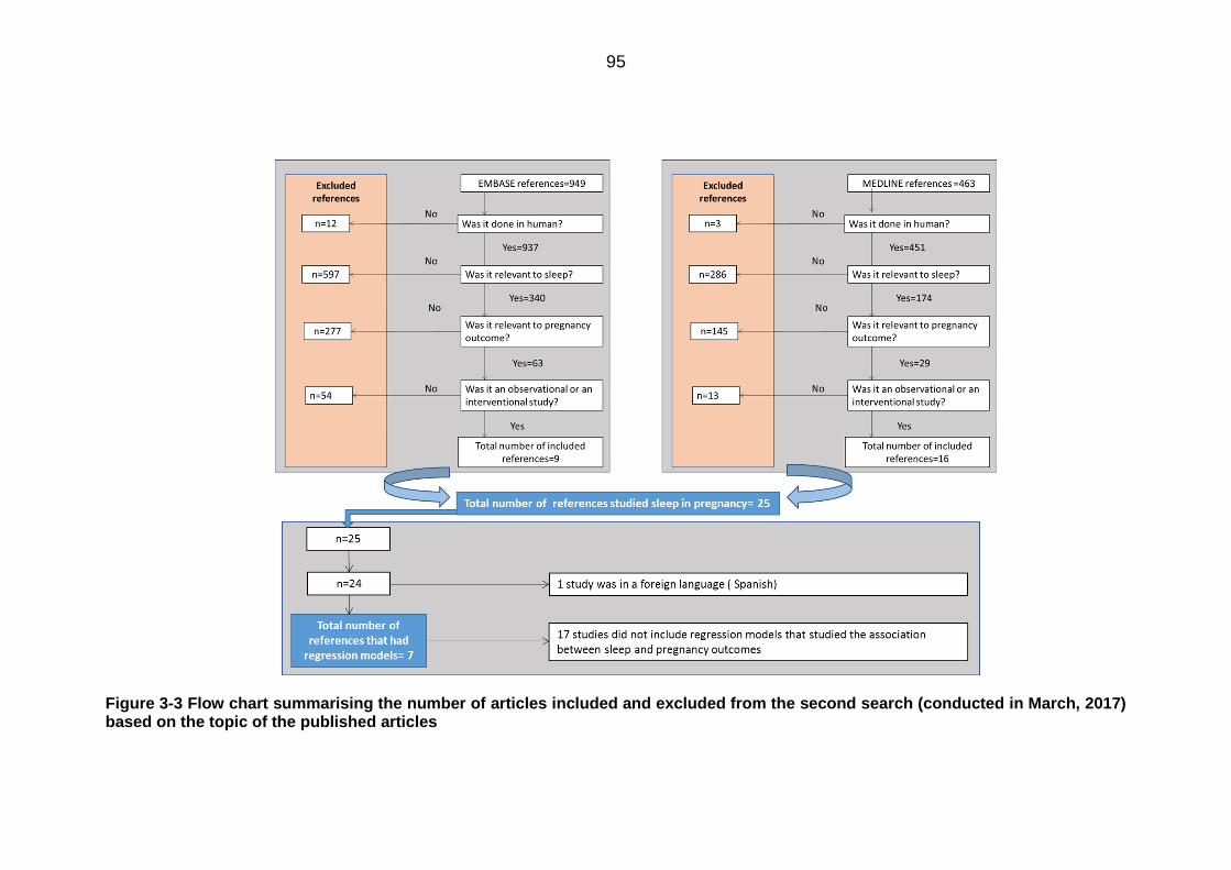
95
Figure 3-3 Flow chart summarising the number of articles included and excluded from the second search (conducted in March, 2017) based on the topic of the published articles

96
3.3.1.1 Study settings and sample sizes
Most of the studies described in the articles included in this review had been
conducted in outpatient antenatal clinics (n = 17), the remainder taking place in
hospital wards (n = 10), national registries (n = 6), and antepartum educational
sessions (n = 1). Approximately 55.88% (n = 19) of the studies included were
conducted in one setting, 11.76% (n = 4) in two settings, and 14.71% (n =5) in
three or more settings; while the remainder 17.65% (n = 6) were those using data
from national registries. The sample sizes of these studies ranged from n=45 to
n=12,506 participants, with an average sample size of n=359 (SD=869)
participants and a total of n=21,911 participants overall. Based on our post hoc
power assessments, the sample size of the majority of studies was insufficient to
achieve an acceptable level of power (as defined at 0.8).
3.3.1.2 Participant characteristics
A complete summary of the key characteristics of each of the studies included in
the systematic review and meta-analyses is presented in Table 3-2.
3.3.1.2.1 Sociodemographic features
The average age of the women examined in these studies was 29.6 years (SD =
5.2, range = 18–47). Their average BMI (at booking) was 27.9 kg/m2 (SD = 5.5,
range = 21–46).
3.3.1.2.2 Inclusion and exclusion criteria
Multiple pregnancy was the most common exclusion criterion, and 52.94% (n=18)
of the studies explicitly included only singleton pregnancies. The second most
common exclusion criterion was previous or current obstetric complication(s), and
47.06% (n = 16) of the studies included only women with a current and/or previous
pregnancy considered healthy (Table 3-1).

97
Table 3-1 Summary of the commonest inclusion and exclusion criteria for studies included in the systematic review.
Common excluded criteria
(Total number =34)
%
Multiparous 2 5.88
Multiple pregnancy 18 52.94
Neonatal death and/or severe neonatal complications 9 26.47
Current or previous obstetric complications 16 47.06
Maternal history of chronic disease 13 38.24
Psychiatric disease or medication 4 11.76
Sleep disorders, travelling across time zones and /or shift work
5 14.71
Obese [pre-pregnancy BMI >30 kg/m2] 3 8.82
Behavioural risks (smoking, caffeine, drug, alcohol) 4 11.76
Can’t speak and/or write in English 8 23.53

98
Table 3-2 Summary of key characteristics for each of the studies included in the systematic review and the meta-analysis.
References Location Sample size Setting Population of interest
Inclusion criteria Exclusion criteria
Retrospective longitudinal studies (n=8)
(Bourjeily et al., 2010)
USA 1000 Delivery ward Women in the 48 hours postpartum period
1. English speakers
2. With or without bed-
partner
1. Women with a neonatal death
(Bourjeily et al., 2013)
USA 1000 University hospital delivery ward
Women in the 48 hours postpartum period
English speakers
1. Women who cannot speak
English
2. Women with neonatal death
(Franklin et al., 2000)
Sweden 502 University hospital OB/GYN ward
Not reported Singleton pregnancy
1. Caesarean delivery
2. Women with a neonatal death
(Louis et al., 2010)
USA Women with OSA =57 Women without OSA =114 Total=171
The Urban tertiary care center Prenatal ward
Women diagnosed with and without OSA who delivered in the urban tertiary care center
Obese (pregnancy BMI ≥
30 kg/𝑚2) or normal weight (pregnancy BMI
between18 and 24 kg/𝑚2)
1. No PSG confirmation of OSA
2. Multiple gestation
(Owusu et al., 2013)
Ghana 234 Korle Bu University Hospital postpartum ward
Women in the 48 hours post-partum period
Women delivered after the 28 week of gestation
Not reported
(Perez-Chada et al., 2007)
Argentina 456 Hospital ‘Donacio n f Santojanni’ Obstetric ward
Pregnant women who came for delivery
Singleton pregnancy
Not reported
(Reid et al., 2011)
Canada 219 Royal university hospital fetal assessment and ante partum ward
Pregnant women with PIH with or without protein urea compared with healthy singleton pregnant women in similar gestational age
Singleton pregnancy
1. Multiple pregnancy
2. Sever underlying maternal or
fetal complications
3. Poorly controlled HTN
4. Diabetes
5. Premature delivery
Chen et al., 2012)
Taiwan Total=4786 Women with OSA=791 Women without OSA=3995
National health insurance database
Women diagnosed as OSA by PSG twice and women never diagnosed with OSA
Singleton pregnancy Not reported

99
References Location Sample size Setting Population of interest
Inclusion criteria Exclusion criteria
Case control studies (n=6)
(Champagne et al., 2009)
Canada Total=50 Cases=17 Control=33
Cases: antenatal admission ward in a tertiary hospital Control: antenatal clinics, ultrasound clinics, antenatal word
Cases: pregnant women with gestational hypertension Controls: pregnant women without gestational hypertension
Controls: 1. ≥20 week of gestation or
a prior month history of delivery
2. Singleton pregnancy
1. Women with pre-gravid hypertension
2. Treated obstructive sleep apnea 3. Neuromuscular disease 4. Previous stroke 5. Women lived >30 Km from the
center 6. Women Lacking English
communication 7. Unstable (intensive care
admission or foetal loss)
(Gordon et
al., 2015)
Sydnee Total=295
Cases=103
Controls=192
Cases and controls:
maternity hospitals in
metropolitan Sydney (9
hospitals)
Cases: Pregnant
women with GA
greater than or
equal to 32 weeks
Control: matched
with cases for
booking hospital and
GA
Cases:
1. Singleton
2. Still birth was in or after
the 32 weeks of
gestation
Controls:
1. Singleton
2. In the 32 weeks of
gestation or greater
Cases and controls;
1. Multiple gestation
2. Fetal with chromosomal
abnormalities or fatal pre-
diagnosed condition
3. Terminated pregnancies
4. Women identified as Aboriginal
or Torres Strait Islander,
(Kajeepeta
et al., 2014)
Peru Total=959
Cases=479
Controls=480
Cases and controls:
Hospital Nacional Dos de
Mayo, the Instituto
Nacional Materno
Perinatal de Lima, and
The Hospital Edgardo
Rebagliati Martins
Cases: women with
spontaneous
preterm delivery
Controls: women
with full term
delivery
Cases:
1. Singleton pregnancies
2. spontaneous births
<,37 weeks (22–36
weeks).
Controls:
Controls:
singleton
term (≥37 weeks
of gestation)
selected from the same
hospital of
delivery.
Cases:
1. Medically indicated premature
births
(Reutrakul et al., 2013)
USA Total=45 Cases=15
Cases: University of Chicago obstetric clinic
Cases: pregnant women with GD
Singleton pregnancy
1. Multiple pregnancy

100
References Location Sample size Setting Population of interest
Inclusion criteria Exclusion criteria
Controls=30
Controls: Advertisement via fliers distributed in university of Chicago medical center
Controls: non-diabetic pregnant women with normal blood glucose level
2. Pre-existing chronic diseases
(DM, sleep disorders,
neurological disorders,
psychiatric disorders, sever
pulmonary, cardiac or renal
diseases)
3. Usage of (steroid, medication
which may affect sleep or
glucose metabolisms,
significant alcohol ≥ 7
drinks/wk, caffeine consumption
≥ 400 mg/d, smoking, durgs)
4. Shift work
5. Recent travel over time zone
(Stacey et al., 2011)
New Zealand
Total=467 Cases=155 Controls=312
Cases: all maternity units in Auckland region Controls: pregnancy registration list from regions where the still birth happened
Cases: pregnant women Women with a history of still birth controls: healthy pregnant women
Not reported 1. Still birth due to congenital
anomalies
2. Multiple pregnancy
(Samaraweera and Abeysena, 2010)
Sri Lanka Cases=230 Controls=504 Total=734
Cases: gynecological ward in De Soysa Maternity Hospital in Sri Lanka Controls: antenatal clinics in De Soysa Maternity Hospital in Sri Lanka
Cases: mothers with a confirmed miscarriage Controls: healthy pregnant ladies in the > 28 weeks of gestation
1. Confirmed partial or
complete miscarriage
2. < 28 weeks of gestation
1. Thyroid disease 2. Major psychiatric disease 3. HTN
Prospective longitudinal studies (n=15)
(Abeysena et al., 2009)
Sri Lanka 690 2 primary health care antenatal clinic in Sri Lanka district
Not reported Not reported 1. Women with GDM or PIH
2. Twin pregnancy
(Abeysena et al., 2010)
Sri Lanka 885 2 primary health care antenatal clinic in the Sri Lanka district
Not reported Not reported 1. Pre-existing DM
2. Pre-existing HTN
3. Epilepsy
4. Psychiatric diseases

101
References Location Sample size Setting Population of interest
Inclusion criteria Exclusion criteria
(Facco et al., 2010)
USA 189 Outpatient clinic in Northwestern Memorial Hospital affiliated practices.
Not reported 1. Nulliparous
2. Singleton pregnancy
1. chronic hypertension
2. Heart disease
3. Chronic lung disease
4. Chronic renal disease
5. Autoimmune disease
(Herring et
al., 2014)
USA 63 Five university outpatient
antenatal clinics
Urban and low-
income pregnant
women
1. < 16 weeks’ gestation
2. Fluency in English or
3. Spanish
4. Currently lives in
Philadelphia
Not reported
(Howe et al.,
2015)
New
Zealand
633 Data from Maternal Sleep
and Health Study in New
Zeland
Women in the third
trimester of
pregnancy (35–37
weeks)
1. Single term
2. Third trimester
Preterm birth
(Ko et al., 2013)
Korea 276 Obstetric outpatient clinics in 2 private hospitals and 3 secondary located hospitals in Soul and its surrounding area
Pregnant women aged 20-45 years
Not reported Not reported
(Lee and Gay, 2004)
USA 131 Child birth educational classes
Not reported 1. First pregnancy
2. Read and write English
1. Diagnosed sleep disorder
2. Work the night shift
3. Previous involuntary pregnancy
lost
Louis et al., 2012)
USA 175 General health and high risk clinics
Obese pregnant women (Pre-pregnancy BMI ≥ 30
kg/𝑚2)
Pre-pregnancy BMI was ≥
30 kg/𝑚2
1. Miscarriage
2. Language barrier
3. Usage of narcotic drugs
4. Usage of any medication that
may affect sleep
5. Non- attendance to three
antenatal visits
(Na-rungsri
et al., 2016)
Thailand 1345 Five prenatal care clinics
affiliated with Maharat
Nakhon Ratchasima
Hospital, which is a large
tertiary hospital
Pregnant women in
the second trimester
1. Singleton pregnancy
2. Started antenatal care
before 20 weeks.
3. Had intention to keep
the pregnancy to term
1. Had asthma
2. Had chronic renal disease
3. Had chronic hypertension
4. Had miscarriages
5. lost on follow-up

102
References Location Sample size Setting Population of interest
Inclusion criteria Exclusion criteria
and to deliver at the
study hospitals were
recruited
(O'Brien et al., 2012)
USA 1719 University of Michigan prenatal clinics
Pregnant women who are in the>28 week
≥ 28 week of gestation Single foetus
Not reported
(O'Brien et al., 2013)
USA 1673 Large tertiary medical center
Pregnant women who were in the third trimester
Not reported Not reported
(Okun et al., 2011)
USA 166 University medical center Pregnant women in the first trimester
1. Singleton pregnancy
2. Non-smoker
3. Do not use any
substance or medication
4. Do not have any
medical condition that
may interfere with their
neuro-endocrine
regularity
5. English speakers
Not reported
(Qiu et al., 2010)
USA 1290 Prenatal medical care clinic at Swedish medical center in Seattle
Healthy Pregnant ladies
1. Started their antenatal
care before the 20th
week of gestation
2. English speaker
3. Planning to complete
her pregnancy period
1. GDM before the study
2. Pregnancy loss
(Reutrakul et al., 2011)
USA 169 (Chicago) Adult pregnant women in the 2nd trimester
Not reported 1. Previous history of GDM
2. Sever diseases (pulmonary,
renal, cardiac)
3. Current neurological disorders
4. Current psychiatric disorders
5. Recent travel over the time
zone
6. Shift work
7. Usage of (steroid, drugs,
smoking, significant alcohol or
caffeine consumptions)

103
References Location Sample size Setting Population of interest
Inclusion criteria Exclusion criteria
8. Medication that may affect
glucose level)
(Sharma et
al., 2016)
India 273 All India Institute of
Medical Sciences
(AIIMS) which is a
tertiary-level referral
center
Pregnant women in
the first trimester
attending AIIMS
OPD
1. Singleton
2. Aged 20 to 40 years
3. First trimester
4. Trophoblastic disease
5. Multifetal gestation
6. Lost to follow-up
7. Had abortions
8. With incomplete data about
perinatal outcomes
(Strange et al., 2009)
USA 220 Antenatal clinics in 15 obstetrical practices
20-29 weeks 1. 20- 29 week of gestation
2. 20-40 years old
3. Reading and
understanding English
1. History of drug abuse
2. History of alcohol abuse
3. History of a diagnosed sleep
disorder
4. History of a psychiatric disorder
5. History of an acute illness
6. History of a chronic illness
(Stinson and Lee, 2003)
359 USA Antenatal care clinics located in 4 military hospitals
Pregnant military women
Singleton gestation
1. History of previous preterm
labor or un intentional
miscarriage
2. History of previous obstetric
complications
3. History of chronic illness
4. History of recently treated
vaginal or urinary tract infection
5. Diagnosed as being in a
preterm labor
(Ugur et al., 2012)
Turkey 465 In-patient obstetric ward or delivery ward in seven hospitals in seven distinct regions (Ankara, Istanbul, Sanliurfa, Erzurum, Rize, Gaziantep)
admitted pregnant women for follow or labor
Not reported Not reported
(Wang et al.,
2017)
China 12 506 antenatal care system of
the urban districts of
Tianjin
Pregnant women
attended antenatal
care in Tianjin
- 1. Women who did not take GCT
2. Women with a positive GCT but
did not take OGTT

104
References Location Sample size Setting Population of interest
Inclusion criteria Exclusion criteria
3. 3. Women with missing
sleepinformation
(Williams et al., 2010)
Sweden 1272 Prenatal medical care clinics at Swedish medical center in Seattle
Healthy pregnant women
1. Started their antenatal
care before the 20th
week of gestation
2. English speaker
3. Planning to complete
her pregnancy period
1. GDM before the study
2. Pregnancy loss

105
3.3.2 Measured variables
3.3.2.1 Sleep characteristics
3.3.2.1.1 Sleep disordered breathing (SDB)
The most commonly studied sleep characteristic was SDB, a characteristic studied
in 22 of the studies reviewed. Snoring and OSA were the two key SDBs covered
therein. Snoring, which was studied in 14 studies, was assessed subjectively using
questionnaires; whilst obstructive sleep apnoea (OSA), which was studied also in
14 studies, was measured either objectively using polysomnography (PSG) or
subjectively using a dedicated OSA-relevant questionnaire.
Various aspects of snoring were considered when studying the relationship
between these and pregnancy outcomes. These included: the onset of snoring
(before vs. during pregnancy), the frequency of snoring, and the presence or
absence of snoring. The effect of chronic snoring (defined as snoring before 28
weeks of pregnancy) was studied in comparison to ‘pregnancy-induced’ snoring
(i.e. snoring after 28 weeks of gestation). In four such studies, the authors
suggested that chronic snoring might be expected to lead to a greater risk of poor
pregnancy outcomes than pregnancy-induced snoring.
The effect of habitual snoring (i.e. snoring that occurred ≥ 3 times per week) was
studied in comparison to non-habitual snoring (< 3 times per week) in no fewer
than 12 studies. The authors of these studies postulated that the effect of snoring
on pregnancy outcomes is likely to become clinically significant once snoring
becomes an ‘habitual’ sleep behaviour – others suggesting that regardless of the
frequency of snoring or its time of onset, the mere presence of snoring could
influences pregnancy outcomes (n= 3). These authors suggested that participants
might over- or underestimate the frequency of their snoring, especially the latter if
they did not have a sleeping partner complaining about their snoring. A participant’s
awareness of their own snoring is therefore likely to be the key indicator of
underlying SDB that achieves a certain (i.e. a noticeable/reportable) degree of
severity.
In a similar vein, obstructive sleep apnoea was considered a severe and advanced-
stage form of SDB when compared to snoring which, in contrast, was considered
merely an indicator of underlying SDB (and not necessarily a severe presentation
or form thereof). Indeed, not all of these studies examined the effect of both snoring
and OSA; some concentrated on one and some on the other. Those studies that
examined OSA primarily concentrated on the presence of OSA rather than its
frequency, as it was suggested that (regardless the frequency of apnoeic attacks)

106
the mere presence of apnoea was likely to be sufficient to cause poor pregnancy
outcomes.
Table 3-3 and Table 3-4 summarise the definitions of SDB used by the studies
included in the present review, together with some summary descriptive statistics
of the study participants therein.

107
Table 3-3 Summary of snoring-related characteristics operationalised as exposures by the studies examined in the review.
Reference Gestational age Measurement Onset of snoring
Reference range Descriptive statistics
Retrospective longitudinal design
(Bourjeily et al., 2010)
Third trimester Questionnaire (MAPI); “In the last 3 months of your pregnancy, how often have you experienced (or were you told) about the following symptoms” “snoring loudly”
Not specified Never or rarely (less than once a week) [reference] Sometimes (1–2 times a week). Frequently (3–4 times a week) or always (5–7 Times a week).
Total participants = 1000 Never\ rarely =483(51%) Sometimes=133(14%) Frequently\ always=333(35%)
(Franklin et al., 2000)
Third trimester Bespoke questionnaire Not specified Non-habitual (often, or always) [reference] Habitual (never, seldom, sometimes)
Total participants=502 Habitual snoring in the last week of pregnancy 23% Occasional snoring during the last week of pregnancy 25%
(Owusu et al., 2013)
Third trimester Bespoke questionnaire “Do you snore loudly?” regardless if it was witnessed or self-noticed
Not specified Absent [reference] Present
Snoring presented in 54 out of 216 (24.0%)
(Perez-Chada et al., 2007)
Not specified Bespoke questionnaire How much have you snored during your pregnancy?
Not specified Non-habitual (Never, seldom or sometimes) [reference] Habitual (often or almost always)
156 out of 456 participants reported habitual snoring (35%).
Prospective longitudinal design
(Howe et al., 2015)
Not specified GSDS questionnaire Chronic snoring vs. pregnancy induced snoring
Non-habitual (<3 times/week) [reference] Habitual snoring (3-4 times /week)
Total participants=633 Number of snorers= 151(23.85%) Number of women started snoring during pregnancy = 104(68.87%) Number of women started snoring before pregnancy = 50(33.11%)
(O'Brien et al., 2012)
Chronic snoring; before the 3rd trimester Pregnancy induced snoring; snoring induced in the third trimester
Pregnancy sleep questionnaire
Chronic snoring vs. pregnancy induced snoring
Non-habitual (<3 times/week) [reference] Habitual snoring (3-4 times /week)
Total participants=1712 Snoring rate was =34.1% 25% started snoring during pregnancy 9% reported chronic snoring
(Qiu et al., 2010)
Not specified Bespoke questionnaire “Since becoming pregnant, when you are asleep, to the
Not specified Non-snorer (some of the time, a little of the time or none of the time)
89 women out of 1290 pregnant women (6.90%) reported snoring in pregnancy
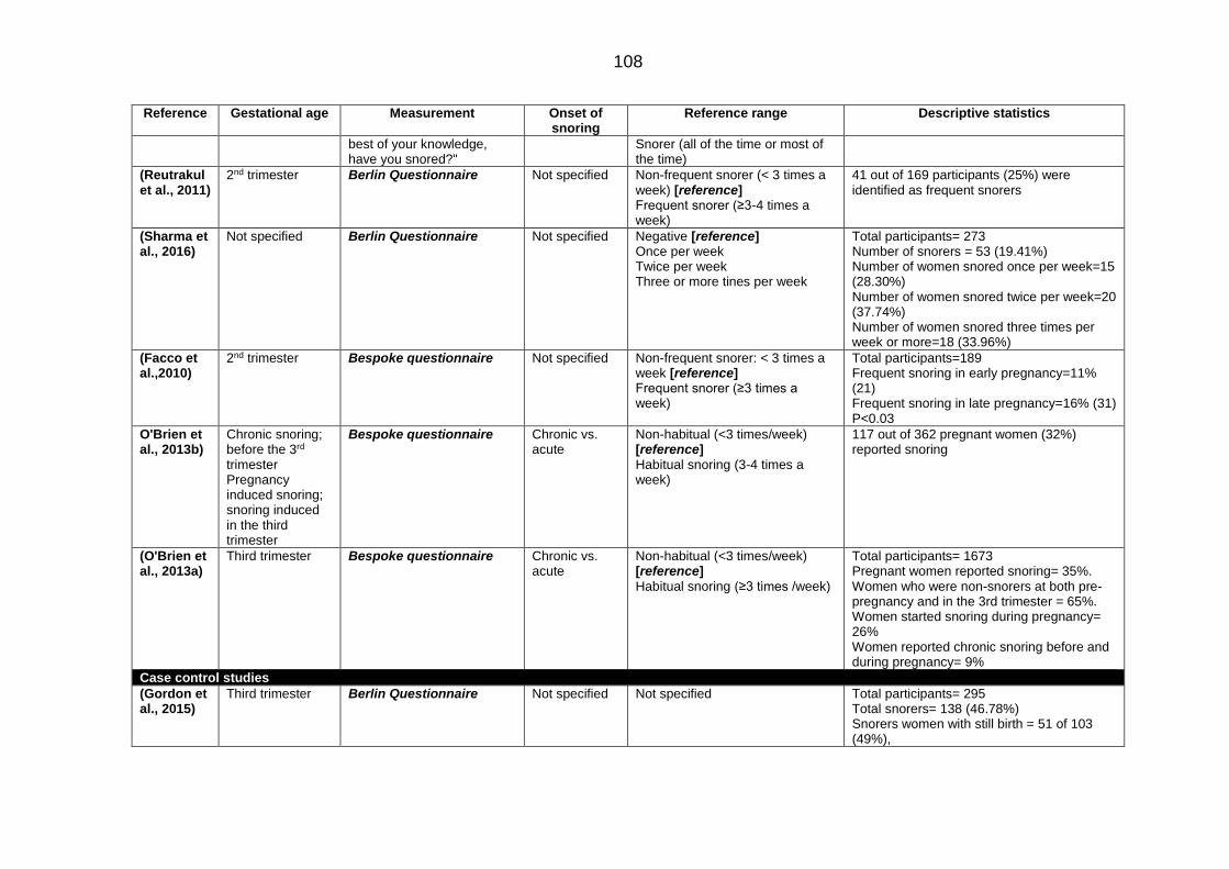
108
Reference Gestational age Measurement Onset of snoring
Reference range Descriptive statistics
best of your knowledge, have you snored?"
Snorer (all of the time or most of the time)
(Reutrakul et al., 2011)
2nd trimester Berlin Questionnaire Not specified Non-frequent snorer (< 3 times a week) [reference] Frequent snorer (≥3-4 times a week)
41 out of 169 participants (25%) were identified as frequent snorers
(Sharma et al., 2016)
Not specified Berlin Questionnaire Not specified Negative [reference] Once per week Twice per week Three or more tines per week
Total participants= 273 Number of snorers = 53 (19.41%) Number of women snored once per week=15 (28.30%) Number of women snored twice per week=20 (37.74%) Number of women snored three times per week or more=18 (33.96%)
(Facco et al.,2010)
2nd trimester Bespoke questionnaire
Not specified Non-frequent snorer: < 3 times a week [reference] Frequent snorer (≥3 times a week)
Total participants=189 Frequent snoring in early pregnancy=11% (21) Frequent snoring in late pregnancy=16% (31) P<0.03
O'Brien et al., 2013b)
Chronic snoring; before the 3rd trimester Pregnancy induced snoring; snoring induced in the third trimester
Bespoke questionnaire
Chronic vs. acute
Non-habitual (<3 times/week) [reference] Habitual snoring (3-4 times a week)
117 out of 362 pregnant women (32%) reported snoring
(O'Brien et al., 2013a)
Third trimester Bespoke questionnaire
Chronic vs. acute
Non-habitual (<3 times/week) [reference] Habitual snoring (≥3 times /week)
Total participants= 1673 Pregnant women reported snoring= 35%. Women who were non-snorers at both pre-pregnancy and in the 3rd trimester = 65%. Women started snoring during pregnancy= 26% Women reported chronic snoring before and during pregnancy= 9%
Case control studies
(Gordon et al., 2015)
Third trimester Berlin Questionnaire Not specified Not specified Total participants= 295 Total snorers= 138 (46.78%) Snorers women with still birth = 51 of 103 (49%),

109
Reference Gestational age Measurement Onset of snoring
Reference range Descriptive statistics
Snorer women with viable birth= 87 of 192 (45%)
(Stacey et al., 2011)
Not specified Not specified Not specified Not specified Number of snorer women who had still birth=
69/155 (45%)
Number of snorer women who had live birth=
130/310 (42%)

110
Table 3-4 Summary of OSA-related characteristics operationalised as exposures by the studies examined in the review.
Reference Gestational age
Measurement Type of apnoea
Reference range Descriptive statistics
Retrospective longitudinal studies
(Bourjeily et al., 2010)
Third trimester
Questionnaire (MAPI); “In the last 3 months of your pregnancy, how often have you experienced (or were you told) about the following symptoms” “stopped breathing”
Self-reported Never or rarely (less than once a week) [reference] Sometimes (1–2 times a week). Frequently (3–4 times a week) or always (5–7 Times a week).
50 participants out of 362 (13.8%) had OSA
(Perez-Chada et al., 2007)
Not specified Bespoke questionnaire Did your partner notice sleep apnoea during your pregnancy?
witnessed apnea
Presence of apnoea Absence of apnoea [reference]
15 out of 447 pregnant women (3.4%) reported witnessed apnoea
(Reid et al., 2011
Third trimester
Full- night polysomnography in sleep laboratory
Measured sleep apnea
Absence of apnoea (respiratory disturbing index(RDI)< 5 events per hour) [reference] Presence of apnoea (RDI ≥ 5 events per hour)
Mean RDI in women with PIH=11.5 (SD=11.2) Mean RDI in women without PIH= 2.3 (SD=3.1) p<0.0002
(Louis et al., 2010)
Not specified PSG Measured sleep apnea
Absence of apnoea (apnoea hypopnea index (AHI) < 5%) [reference] Presence of apnoea ((AHI)≥ 5%)
Total participants=171 Women without OSA = 114 Women with OSA = 57 Diagnosis of OSA amongst women with OSA: Before pregnancy=33 (58%) During pregnancy= 24 (42%)
(Ugur et al., 2012)
Not specified Berlin questionnaire Risk of OSA Not reported 69 women out of 465 women had positive risk of OSA (14.4%)
Case control studies
(Champagne et al., 2009)
>20 weeks Unattended over one night PSG Done at home or hospital
Pregnancy induced apnea Measured sleep apnea
Absence of apnoea (apnoea hypopnea index (AHI) < 15%) [reference]
Presence of apnoea (AHI)≥ 15%
Total participants=50 The rate of OSA was 14 out of 17 (82%) among the hypertensive pregnant women compared with 15 out of 33 (45%) among the normotensive pregnant women.
(Gordon et al., 2015)
≥32 weeks Berlin Questionnaire Subjective OSA
Not defined Total participants = Total number of women with apnea symptoms=34 13 out of 192 women with no still birth had OSA symptoms (11%) 21 out of 103 women with still birth had OSA symptoms (12%)

111
Reference Gestational age
Measurement Type of apnoea
Reference range Descriptive statistics
(Reutrakul et al., 2013)
Late second to early third trimester
PSG over night Measured OSA
Absence of apnoea (apnoea hypopnea index (AHI) < 5%) [reference] Presence of apnoea ((AHI)≥ 5%)
Total participants=45 15 out of 30 women had OSA (50%) 11 from the 15 GDM women (73%) were diagnosed with OSA, 4 from the 15 pregnant without GDM (27%) were diagnosed with OSA P<0.01
Prospective longitudinal studies
(Chen et al., 2012)
Not specified Polysomnography Measured OSA Absence of apnoea [reference] Presence of apnoea
Total participants=4786 Women without OSA= 3955 Women with OSA =791
(Ko et al., 2013)
Not specified Berlin Questionnaire Self-reported OSA
Absence of apnoea risk [reference] Presence of apnoea risk
Total participants=276 Total prevelence of OSA = 32.6% Prevelence of OSA in non- obese women = 43.6% Prevelence of OSA in obese women= 28.3% P=0.001
(Louis et al., 2012)
Not specified In home portable PSG overnight
Measured OSA
Absence of apnoea (apnoea hypopnea index (AHI) < 5%) [reference] Presence of apnoea ((AHI)≥ 5%)
AHI median=12.9 events/hour Total participants=175 OSA rate=15.4% CI 95%= 10.4–21.6%
(Na-rungsri et al., 2016)
2nd trimester Berlin Questionnaire Subjective OSA
Not reported Rate of women with high risk OSA =10.1% (n = 136)
(Reutrakul et al., 2011)
2nd trimester Berlin Questionnaire Subjective OSA
Not reported 29% 48/169 women had an increased risk of SDB
(O'Brien et al., 2013)
Third trimester
Bespoke questionnaire “had stopped breathing/gasped for air at night.”
Subjective OSA
Absence of apnoea (never) [reference] Presence of apnoea (often, usually, always, almost always)
Total participants=1673 Total women had either stopped breathing or air gasping= 3.1%

112
3.3.2.1.2 Sleep duration
Sleep duration was the second most-commonly studied sleep characteristic, and
was examined in 10 of the studies reviewed.
‘Normal’ sleep duration was defined using a range of different cut-off points by the
authors of different studies (Table 3-5). In general, the range of the ‘normal’ sleep
duration considered suitable as a reference value was between 6 and 10 hours, as
measured at different gestational ages of pregnancy, and primarily using subjective
questionnaires – except in the studies by Lee and Gay (2004) and Herring et al
(2014) in which wrist-worn actigraphs were used.
3.3.2.1.3 Sleep quality
Sleep quality was examined by a total of 6 studies, all of which used subjective
measurement tools. Sleep quality was either assessed by using a single question
or measured by the frequency of unfavourable sleep phenomena. For example,
two studies measured sleep quality using the Pittsburgh Sleep Quality Index
(PSQI), which defined sleep quality based on seven sleep characteristics: duration,
efficiency, latency, disturbance, daytime dysfunction, usage of medication, and
subjective sleep quality (Okun et al., 2011, Reutrakul et al., 2011). Three studies
used the general sleep disturbance scale (GSDS), designed to measure the level
of sleep disturbance by concentrating on how frequently respondents had difficulty
of falling sleep, the duration of sleep latency, the frequency of waking in the middle
of the night, the frequency of waking early in the morning, the use of sleep-related
medication, and the subjective assessment of sleep quality (Sharma et al., 2016;
O'Brien et al., 2013, Stinson and Lee, 2003) – i.e. in a very similar fashion to the
PSQI. Finally, two studies used a bespoke question to assess the subjective quality
of sleep without measuring any of the other sleep characteristics’ contributions to
‘quality’ (Wang et al., 2017, Lee and Gay, 2004; Table 3-6).
3.3.2.1.4 Sleep disturbance
Two studies included in the systematic search examined the association between
sleep disturbance and pregnancy outcomes (Table 3-7). Sleep disturbance was
measured subjectively in the first (by Stacey et al. 2011), in which it was defined
as fragmented sleep secondary to toilet use during the night. The second, by Lee
and Gay (2004), examined sleep disturbance using an wrist-worn actigraph and
defined disturbance as a wakeup time after sleep onset (WASO) that exceeded
15% of the total sleep time (Table 3-7).

113
3.3.2.1.5 Excessive daytime sleepiness
Three studies examined the association between daytime sleepiness and
pregnancy outcomes (Table 3-8). Daytime sleepiness was measured using the
Epworth sleepiness scale (ESS) in two studies (Bourjeily et al., 2013, Reutrakul et
al., 2011), though these studies used different reference points to define excessive
daytime sleepiness (Table 3-8). The third study, by Stacey et al. (2011) measured
daytime sleepiness using a bespoke questionnaire, but did not define the reference
point they used to characterise excessive daytime sleepiness (Table 3-8).
3.3.2.1.6 Sleep position
Three studies examined the association between sleep position and pregnancy
outcomes (
Table 3-9). Stacey et al. (2011) used the left-side sleep position as the referent
for lower risk, while Owusu et al. (2013) and Gordon et al. (2015) examined the
risk of the supine position against all other positions (
Table 3-9).

114
Table 3-5 Summary of sleep duration-related characteristics operationalised as exposures by studies examined in the review.
Reference Measurement tool
Trimesters Sleep deprivation (hours/nigh
t)
Short sleep (hours/nigh
t)
Normal sleep
(hours/night)
Long sleep (hours/nigh
t)
Descriptive results
Case control studies
(Kajeepeta et al., 2014)
“During the first 6 months of your pregnancy, how many hours per night did you sleep?”
The first 6 months of pregnancy
<6 7-8 >9 Short sleep duration rate= 22.3% among preterm cases and 16.5% among term controls long duration rate= 18.4% among preterm cases and 15.8% in terms controls.
(Stacey et al., 2011)
“the usual duration of sleep at night during the last month”
After second trimester
- < 6 6-8 > 8 -
(Reutrakul et al., 2011)
PSQI Not specified <7 - - -
(Samaraweera and Abeysena, 2010)
“the total hours of sleep per day”
Not specified
- < 8 ≥ 8 -
Prospective longitudinal studies
(Abeysena et al., 2009)
Physical activity questionnaire
Not specified
- ≤8 - - -
(Abeysena et al., 2010)
Physical activity questionnaire
Not specified
- ≤8 > 8 - -
(Facco et al., 2010)
“During the past month, how many hours of actual sleep did you get at night?”
Not specified
- < 7 - - -
(Howe et al., 2015) Bespoke questionnaire Third trimester - ≤6 7-8 ≥9 -
(Herring et al., 2014)
Actigraph watch 2nd trimester - - - - Mean sleep duration=6h 09 min (SD = 09 min)
(Lee and Gay, 2004)
Actigraph watch Third trimester < 6 < 7
7-8 > 8 Mean sleep duration= 7h10min (SD = 1h10min).

115
Reference Measurement tool
Trimesters Sleep deprivation (hours/nigh
t)
Short sleep (hours/nigh
t)
Normal sleep
(hours/night)
Long sleep (hours/nigh
t)
Descriptive results
(Qiu et al., 2010) "Since becoming pregnant, how many hours per night do you sleep?"
First trimester ≤ 4 5-8 9 ≥ 10
(Wang et al., 2017)
“How many hours of sleep did you get every day during the index pregnancy, including both day and night time?”
Not specified - <7 7-8 ≥9 The median sleep duration was 9 h.
(Williams et al., 2010)
“Since becoming pregnant, how many hours per night do you sleep?”
First trimester < 6 5-6 9 ≥ 10

116
Table 3-6 Summary of sleep quality-related characteristics operationalised as exposures by studies examined in the review.
Gestational age Sleep quality measurement tool
Used question Reference point Measured component of sleep quality
Descriptive statistics
Prospective longitudinal studies
(Howe et al., 2015) Third trimester GSDS Global score Good sleep quality=global score <3
Duration, latency, disturbance, day sleepiness, medication, subjective quality
86.6% (n=380) of mother identifies as Maori (N=194) had poor quality 86.1% (n=167) of mother identifies as non-Maori (N=439) had poor quality
Single question Non-problematic quality <3 nights per week
Subjective quality 82.9% (n=364) of mother identifies as Maori (N=194) had poor quality 84% (n=163) of mother identifies as non-Maori (N=439) had poor quality
(Lee and Gay, 2004)
Third trimester A bespoke question
The question formula was not mentioned
was not defined subjective sleep quality assessment
Not reported
(Okun et al., 2011) Third trimester PSQI Global score
Good quality sleep= global score ≤5
Duration, efficiency, latency, disturbance, day-dysfunction, medication, subjective quality
Mean PSQ according to trimesters In women with preterm delivery 1st =7.8(SD=4.9) 2nd=6.2(SD=4.0) 3rd=7.8(SD=4.1) In women with term delivery 1st=5.0(SD=2.7) 2nd=5.0(SD=2.6) 3rd=5.3(SD=2.7) P<0.03
(Reutrakul et al., 2011)
Second trimester PSQI Global score Good quality sleep= global score ≤5
Duration, efficiency, latency, disturbance, day dysfunction, medication, subjective quality
64% of 169 women had poor sleep quality Mean PSQI = 7.4 ± 4.0
(Stinson and Lee, 2003)
Second trimester GSDS Global score Good sleep quality=global score <3
Duration, latency, disturbance, day sleepiness, medication, subjective quality
Mean GSDS In women with preterm delivery 43.7(SD=16.5)

117
Gestational age Sleep quality
measurement tool
Used question Reference point Measured component of sleep quality
Descriptive statistics
Prospective longitudinal studies
In women with term delivery 49.8(SD=15.5
(Wang et al., 2017) Not specified ‘How did you feel about your sleep quality during the index pregnancy: good, moderate or poor?’
Good Moderate Poor
Good Subjective quality 37.9% of women reported good quality, 59.9% of women reported moderate quality 2.2% of women reported poor quality
Table 3-7 Summary of sleep disturbance-related characteristics operationalised as exposures by the studies examined in the review.
Gestational age measurement tool Reference point Measured component of sleep Descriptive results
Case control studies
(Stacey et al., 2011) Third trimester A bespoke question Not defined “Frequency of getting up to the toilet” over the last month”
Not mentioned
Prospective longitudinal studies
(Lee and Gay, 2004) Third trimester Actigraph watch WASO ≥ 15% WASO Women with WASO≥ 15%=41 (31.30%)

118
Table 3-8 Summary of daytime sleepiness-related characteristics operationalised as exposures by the studies examined in the review.
Gestational age measurement tool Reference point Descriptive results
Retrospective longitudinal studies
(Bourjeily et al., 2013)
Not specified ESS Excessive day time sleepiness >10
Total participants= 1000 ESS mean score (p< 0.0001) Women with snoring= 6.6 Women without snoring = 7.9 ESS > 10 (p<0.0002). 25.5 % of women had snoring, (n=329) 15.3 % of women did not have snoring (n=610)
Case control studies
(Stacey et al., 2011) Third trimester Bespoke questionnaire
Not defined Total participants=467 78 of women with still birth (n=155) reported regular day sleepiness whilst 116 women from the 310 women who did not had still birth reported regular day sleepiness p<0.006
Prospective longitudinal studies
(Reutrakul et al., 2011)
Second trimester ESS Normal score ≤8 41% of 169 women had excessive day time sleepiness
Table 3-9 Summary of sleep position-related characteristics operationalised as exposures by the studies examined in the review.
Reference Gestational age Measurement tool Reference sleep position
High risk sleep position
Descriptive results
Retrospective longitudinal studies
(Owusu et al., 2013) Not specified Bespoke questionnaire While pregnant, what is your most common sleep position?
Not defined Supine position 21 out of 216 (9.7%) reported supine sleep position
Case control studies
(Stacey et al., 2011) Last night of pregnancy
Bespoke questionnaire Left side All others positions
From the 287 pregnant women 61% (n=174) women slept on their left side, 46% (n=133) on their right side and 10% (n=30) on their back.
(Gordon et al., 2015)
≥ 32 weeks Bespoke questionnaire Not defined Supine position Supine position rate was 9.71% (10 of 103) in women with still birth 2.08% (4 of 192) in women viable birth

119
3.3.2.2 Measured birth outcomes
3.3.2.2.1 Neonatal pregnancy outcomes
Foetal growth was studied by studies included in the review using two different
though related concepts: small for gestational age (SGA) being examined in six
studies and low birth weight (LBW) in four. Newborn health and well-being were
measured in three studies using Apgar scores and by admission to the neonatal
intensive care unit (NICU) in two.
SGA was defined by Franklin et al. (2000) as a birth weight below 2 standard
deviations of the median value in the Sweden infant weight reference charts; whilst
it was defined by Howe et al. (2015), Ko et al. (2013), Bourjeily et al. (2010) and
Abeysena et al. (2009) as simply a birth weight <10th percentile after adjusting for
foetal sex and gestational age at birth. O'Brien et al. (2013) further scaled the birth
weight to maternal height, weight, ethnic origin, and parity (essentially adjusting
birth weight by each of these preceding maternal covariates). Low birth weight
(LBW) was examined by the studies authored by Sharma et al. (2016), Owusu et
al. (2013), Chen et al. (2012) and Abeysena et al. (2010). In all of these studies
LBW was defined as a birth weight below 2500g as measured immediately after
birth without adjusting for gestational age at birth or the sex of the newborn. The
Apgar scores used were those measured immediately after birth (Bourjeily et al.,
2010) and those measured 5 minutes thereafter (Sharma et al., 2016, Chen et al.,
2012, Bourjeily et al., 2010). These two measurements were studied in relation to
sleep using a value of ≥7 as the reference cut-off score.
NICU admission was reported regardless of the reason for admission or the length
of stay, though only in two of the studies reviewed (Reutrakul et al., 2011, Louis et
al., 2010).
Finally, fatal foetal outcomes were assessed using reports of miscarriage and
stillbirth; miscarriage being defined by Samaraweera and Abeysena (2010) as
partial or full expulsion of the foetus during the first 28 weeks of gestation.
Gordon et al. (2015), Owusu et al. (2013) and Stacey et al. (2011) examined the
association between stillbirth and several unfavourable sleep events. Stacey et al.
(2011) defined stillbirth as the birth of a baby that had died in utero during the
antenatal or intrapartum periods during/or after 28 weeks gestation, and did not
suffer from congenital anomalies. In contrast, Gordon et al. (2015) included only
those neonatal deaths that occurred during/or after 32 weeks gestation.
120
Since stillbirth and miscarriage are both extremely traumatic to mothers, a few of
the studies explicitly excluded women with histories of these phenomena
(Champagne et al., 2009).
3.3.2.2.2 Maternal pregnancy outcomes
The following maternal pregnancy outcomes were examined in relation to sleep by
studies included in the review: gestational diabetes (GDM), pregnancy-induced
hypertension (PIH), pre-eclampsia (PE), preterm delivery, and caesarean delivery
(Table 3-10 and Table 3-11).
Eight references studied GDM as the outcome of interest, diagnosed using the
100g OGTT test. However, not all of these studies reported their GDM criteria
(Table 3-10). Indeed, one study (Wang et al. 2017) used a 75g OGTT test to
diagnose GDM in their study, whilst Herring et al. (2014) used a 50g non-fasting
OGTT to diagnose hyperglycaemia rather than GDM.
Preterm delivery was defined as delivery before 37 weeks of gestation and was
examined by 4 separate studies.
As for complications with delivery, the risk of elective and/or emergency caesarean
delivery was examined in comparison to spontaneous or assisted vaginal delivery.
Emergency caesarean delivery was examined separately (i.e. not in conjunction
with elective caesarean delivery) in just one reference (Bourjeily et al., 2013).
Elective caesareans are important to examine separately since these may be likely
to be decisions taken due to causes that occurred prior to the measurement of
sleep – such as uterine abnormalities or a previous history of caesarean delivery.
In addition, elective caesarean delivery may be secondary to causes that follow
sleep measurement (such as excessive foetal growth or breech position).
However, examining caesarean deliveries alongside emergency caesareans
would not necessarily cause confounding bias, but it might cause measurement
error or mediation bias.
Pregnancy-induced hypertension (also known as gestational hypertension), which
is a key component of pre-eclampsia, was examined in relation to sleep in a total
of 12 different studies (Table 3-10), 5 of which distinguished PIH from PE (Ko et
al., 2013, Owusu et al., 2013, Ugur et al., 2012, Louis et al., 2012, Williams et al.,
2010). In these studies, pre-eclampsia was defined as elevated blood pressure
after 20 weeks of gestation with a diastolic reading >90 mmHg or a systolic reading
>140 mmHg plus proteinuria of >300 mg/24 hr. In contrast, PIH was defined as
elevated blood pressure after 20 weeks of gestation with or without proteinuria.
.

121
Table 3-10 Summary of pregnancy outcomes examined by studies included in the review.
Reference Used definition Descriptive statistics
Small for gestational age
Retrospective longitudinal
(Bourjeily et al., 2010) Birth weight “<10th percentile for gestational age” Not reported
(Franklin et al., 2000) “Birth weight below two standards deviation in the Sweden infant weight charts”
Total participants=502 7% of 113 habitual snorers gave a birth to SGA infant 2.6% of 389 non- habitual snorers gave a birth for SGA (p<0.05
Prospective longitudinal study
(Abeysena et al., 2009) Birth weight < 10th percentile adjusted for maternal height, feeding requirement, foetal sex, GA, ethnicity and maternal weight
Mean birth weight= 2946 g
(Howe et al., 2015) Birth weight “<10th percentile for gestational age” Total participants=633 Rate of SGA was 8.85% (n=56) Rate of SGA in mother identifies as Maori (N=194) was 6.7% (n=13) Rate of SGA in mother identifies as non-Maori (N=439) was 9.8% (n=43)
(Ko et al., 2013) “<10th percentile adjusting for foetal sex and gestational age”
17 participants of 276 total participants (6.16%) give a birth to SGA neonates
(O'Brien et al., 2013) Birth weight < 10th centile adjusted for maternal height, maternal weight, ethnic origin, parity, infant sex, gestational age
Birth weight < 10th centile =12.5% of total 1673 participants
Low birth weight
Retrospective longitudinal study
(Owusu et al., 2013) Birth weight< 2500 g at birth Total participants=234 6 out of 53 snorers had low birth babies (11.3%) 21 out of 167 non-snorers had low birth weight babies (12.6%) :
Prospective longitudinal study
(Abeysena et al., 2010) Birth weight< 2500 g at birth Mean= 2946± 473 g 87 LBW babies (11.8%) from 885 babies
(Chen et al., 2012) Birth weight< 2500 g at birth Mean birth weight Women with OSA= 306 (SD=584) g Women without OSA=3147(SD=418) g 233 women from the 4746 (4.91%) had LBW babies
(Sharma et al., 2016) Birth weight< 2500 g at birth Total participants= 273 Rate of LBW was 31.14 % (n=85)
Apgar score
Retrospective longitudinal study
(Bourjeily et al., 2010) 1-min. and 5-min. low Apgar scores (<7) Not reported

122
Reference Used definition Descriptive statistics
Prospective longitudinal study
(Chen et al., 2012) 5-min. low Apgar scores (<7) Total participants=4786 Women with OSA=10 (1.3%) Women without OSA= 5(0.1%) P<0.001
(Sharma et al., 2016) 5-min. low Apgar scores (<7) Not reported
NICU admission
Prospective longitudinal study
(Reutrakul et al., 2011) Not reported Not reported
(Louis et al., 2012) Not reported 12 (46.1%) women with OSA reported NICU admission 24 (17.8%) women without OSA reported NICU admission
Still birth and miscarriage
Retrospective longitudinal studies
(Owusu et al., 2013) Not reported 2 out of 53 snorers had a still birth delivery (3.8%) 7 out of 53 non –snorers had a still birth delivery
Case control study
(Samaraweera and Abeysena, 2010)
“partial or full expulsion of the foetus during the first 28 weeks of gestation”
Women with miscarriage 230 Women without miscarriage 501 Amongst women with miscarriage: 1st trimester miscarriage= 91/230 women (39.5%) 2nd trimester miscarriage= 139/230 women (60.4%)
(Stacey et al., 2011)
“Stillbirth was defined as the birth of a baby that died in utero during the antenatal or intrapartum periods” GA= ≥ 28 week
Pregnant women experienced late still birth = 215 Prevalence of still birth = 3.09/1000 births The absolute risk of late stillbirth = 3.09/1000 95% CI= 2.70 to 3.53/1000
(Gordon et al., 2015) Late still birth during or after 32 weeks of gestation Women with still birth =103 Women with viable birth= 192
Gestational diabetes
Prospective longitudinal study
(Qiu et al., 2010)
If one of the following results was positive using 100 grams, 3-hour OGTT
• fasting ≥ 95 mg/dl
• 1-hour ≥ 180 mg/dl
• 2-hour ≥ 155 mg/dl
• 3-hour ≥140 mg/dl.
68 /1290 women (5.3%) developed GDM
(Reutrakul et al., 2011) The test was done using 100-g OGTT But no cut off point was reported
26 women (15%) had GDM
(Facco et al., 2010) The test was done using 100-g OGTT But no cut off point was reported
9 out of the 88 women With short sleep duration (10.2%) and 1 out of the 94 women Without short sleep duration (1.1%) were diagnosed with GDM P<0.008

123
Reference Used definition Descriptive statistics
(Chen et al., 2012) Not reported Women with OSA=37 (4.7%) Women without OSA=130 (3.3%) P<0.053
(Herring et al., 2014) Hyperglycemia was identified if the blood glucose level was ≥130 mg/dL using 50-g non-fasting OGTT with 1 hour sample
From the 63 participants 7 women (11%) were classified with hyperglycemia
(O’Brien et al., 2012) Not reported 19%women from 584 women with snoring had GDM 15 %women from the1128 non- snorer women had GDM
(Reutrakul et al., 2013) Using 100-g OGTT Two abnormal readings Using 1- hour glucose tolerance test with 50 g OGTT Blood glucose=≤ 140 mg/dl Blood glucose =≥ 200 mg/dl
Pregnant women with GDM= 15 Pregnant women without GDM= 15
(Sharma et al., 2016) American Diabetes Association criteria Total participants= 273 Rate of women diagnosed of GDM= 14.65 % (n=40)
(Wang et al., 2017) Using 75-g OGTT GDM was diagnosed if one of the following Fasting glucose ≥ 5.1 mmol/l 1-h plasma glucose ≥ 10.0 mmol/l 2-h plasma glucose ≥ 8.5 mmol/l
7.3% (n=919) women had gestational diabetes
Retrospective longitudinal
(Bourjeily et al., 2013) American Diabetes Association criteria 94 (10%) women had GDM
(Bourjeily et al., 2010) Not reported 98 (9.8%) of women had GDM
Mode of delivery
Prospective longitudinal study
(Lee and Gay, 2004) Both Elective and emergency caesarean General vaginal birth= 62% Assisted vaginal birth=17% Caesarean section=21%
(O'Brien et al., 2013) Emergency caesarean or Elective caesarean
Emergency CS= 19.4% Elective CS= 18.2%
(Chen et al., 2012) Both Elective and emergency caesarean Women with OSA=399 (50.4%) Women without OSA=1475(37.3%) P<0.01
(Ko et al., 2013) Both Elective and emergency caesarean From 89 women with OSA 32 had caesarean delivery (36%) From187 women without OSA 42 (22.5%) caesarean delivery
(Louis et al., 2012) Both Elective and emergency caesarean Total Caesarean delivery= 64 women 38% Elective caesarean=40%
(Sharma et al., 2016) Both Elective and emergency caesarean Total participants= 273 Rate of CS was 28.57 % (n=78)
Retrospective longitudinal
(Bourjeily et al., 2013) Elective caesarean 498 (53%) women had vaginal delivery 305 (32.5%) women had Caesarean delivery

124
Reference Used definition Descriptive statistics
(Bourjeily et al., 2010) Emergency caesarean 5.4% had Caesarean delivery
Preterm delivery
Prospective longitudinal study
(Louis et al., 2012) Delivery before 37 weeks From the 89 women with OSA 5 (17.6%) had preterm delivery From the 187 women without OSA 26 (18.5 %) had preterm delivery
(Louis et al., 2010) Not defined From the 57 women with OSA 17 (29.8%) had preterm delivery From the 114 obese women11 (9.6 %) had preterm delivery From the 114 normal weight women 14 (12.3%) had preterm delivery
(Stinson and Lee, 2003) Not reported 50 participants had preterm delivery (13.9%)
(Okun et al., 2011) Delivery before 37 weeks Preterm delivery= 15 (9.0%) Term delivery= 151 (91%)
(Na-rungsri et al., 2016) Delivery before 37 weeks and was divided into
Total participants= 1345 Preterm delivery= 143 (10.63%) Term delivery= 1197(88.99%)
(Reutrakul et al., 2011) Not reported Not reported
(Strange et al., 2009) Not reported Total preterm birth= 14.6%
Retrospective longitudinal
(Bourjeily et al., 2010) Delivery before 37 weeks 12% women from 1000 participants had preterm delivery
Case control (Kajeepeta et al., 2014) Spontaneous and not medically indicated delivery that happened before 37 weeks and after 22 weeks of gestation
Women with preterm delivery =479 Women with term delivery =480
Pre-eclampsia
Prospective longitudinal
(Williams et al., 2010) Not reported Not reported
(O'Brien et al., 2012) Not reported 12.9% from 584 snorers had PE 8.2% from 1128 non-snorers had PE
(Ko et al., 2013) Systolic BP>140 mmHg or diastolic BP>90mmHg Measured 2 times within 4-14 days apart plus protein urea >300gm/dl
3 of 89 women with OSA had PE 6 of 187 women without OSA had PE
(Louis et al., 2012) New onset HTN (GA >20 week) in previously normal women Bp>140/90 mmHg Proteinuria> 300 mg/24 hours
23 (16.9%) women without OSA had PE 11 (42.3%) women with OSA had PE
(Ugur et al., 2012) Not reported 18 (5%) women without OSA (n=396) had PE 19 (23%) women with OSA (n=69) had PE
Retrospective longitudinal
(Franklin et al., 2000) pregnancy-induced hypertension with proteinuria ≥ 300 mg/24 hour
Total 26 cases of PE 10% in habitual snorer 4% in non habitual snorer p<0.05
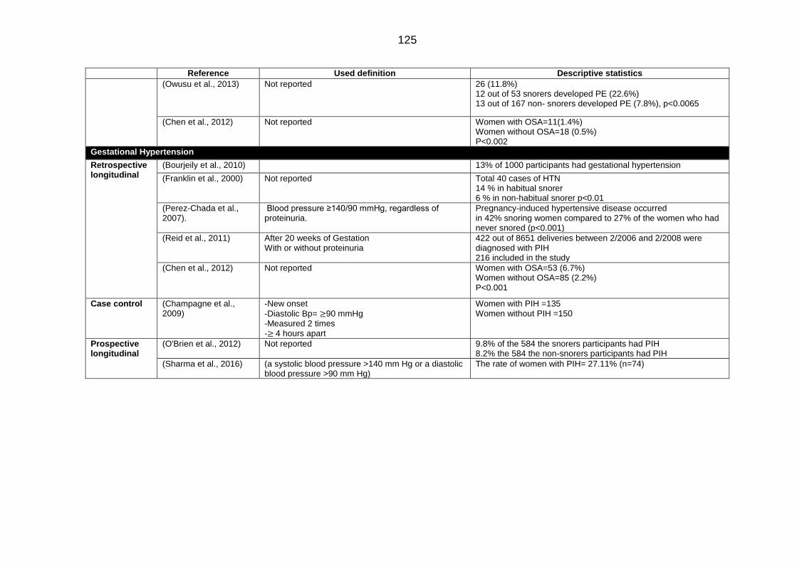
125
Reference Used definition Descriptive statistics
(Owusu et al., 2013) Not reported 26 (11.8%) 12 out of 53 snorers developed PE (22.6%) 13 out of 167 non- snorers developed PE (7.8%), p<0.0065
(Chen et al., 2012) Not reported Women with OSA=11(1.4%) Women without OSA=18 (0.5%) P<0.002
Gestational Hypertension
Retrospective longitudinal
(Bourjeily et al., 2010) 13% of 1000 participants had gestational hypertension
(Franklin et al., 2000) Not reported Total 40 cases of HTN 14 % in habitual snorer 6 % in non-habitual snorer p<0.01
(Perez-Chada et al., 2007).
Blood pressure ≥140/90 mmHg, regardless of proteinuria.
Pregnancy-induced hypertensive disease occurred in 42% snoring women compared to 27% of the women who had never snored (p<0.001)
(Reid et al., 2011) After 20 weeks of Gestation With or without proteinuria
422 out of 8651 deliveries between 2/2006 and 2/2008 were diagnosed with PIH 216 included in the study
(Chen et al., 2012) Not reported Women with OSA=53 (6.7%) Women without OSA=85 (2.2%) P<0.001
Case control (Champagne et al., 2009)
-New onset
-Diastolic Bp= ≥90 mmHg -Measured 2 times -≥ 4 hours apart
Women with PIH =135 Women without PIH =150
Prospective longitudinal
(O'Brien et al., 2012) Not reported 9.8% of the 584 the snorers participants had PIH 8.2% the 584 the non-snorers participants had PIH
(Sharma et al., 2016) (a systolic blood pressure >140 mm Hg or a diastolic blood pressure >90 mm Hg)
The rate of women with PIH= 27.11% (n=74)

126
Table 3-11 Summary of the studies included in the review together with the (sleep-related) exposures and (pregnancy outcome-related) outcomes examined.
Sleep duration Sleep quality Sleep disturbance Day sleepiness Latency Sleep Position
Snoring OSA
Neonatal outcomes
SGA (Abeysena et al., 2009)
(Howe et al., 2015)
(Howe et al., 2015)
(Franklin et al., 2000)
(Bourjeily et al., 2010)
(Howe et al., 2015)
(Ko et al., 2013) (O'Brien et al.,
2013)
LBW (Abeysena et al., 2010)
(Owusu et al., 2013).
(Sharma et al., 2016)
(Chen et al., 2012)
Apgar Score (Sharma et al., 2016)
(Bourjeily et al., 2010)
(Chen et al., 2012)
NICU admission (Reutrakul et al., 2011)
(Louis et al., 2012)
Miscarriage (Samaraweera and Abeysena, 2010)
Still birth (Stacey et al., 2011).
(Stacey et al., 2011).
(Stacey et al., 2011)
(Owusu et al., 2013)
(Stacey et al., 2011)
(Gordon et al., 2015)
(Stacey et al., 2011)
(Gordon et al., 2015)
(Gordon et al., 2015)
Maternal and perinatal outcomes
GDM (Qiu et al., 2010) (Reutrakul et al.,
2011) (Facco et al., 2010) (Wang et al., 2017)
(Herring et al., 2014)
(Wang et al., 2017)
(Qiu et al., 2010) (Reutrakul et al.,
2011) (O’Brien et al.,
2012) (Facco et al.,
2010) (Bourjeily et al.,
2010)
(Reutrakul et al., 2011)
(Chen et al., 2012) (Reutrakul et al.,
2013) (Bourjeily et al.,
2010)

127
Sleep duration Sleep quality Sleep disturbance Day sleepiness Latency Sleep Position
Snoring OSA
Mode of delivery (Lee and Gay, 2004)
(Lee and Gay, 2004)
(Lee and Gay, 2004)
(Bourjeily et al., 2013)
(O'Brien et al., 2013)
(Bourjeily et al., 2010)
(Sharma et al., 2016)
(Chen et al., 2012) (Ko et al., 2013)
(Louis et al., 2012) (Bourjeily et al.,
2010)
Preterm delivery (Kajeepeta et al., 2014)
(Stinson and Lee, 2003)
(Okun et al., 2011) (Reutrakul et al.,
2011)
(Reutrakul et al., 2011)
(Strange et al., 2009)
(Bourjeily et al., 2010)
(Louis et al., 2012) (Louis et al., 2010) (Na-rungsri et al.,
2016
PE (Williams et al.,2010)
(Franklin et al., 2000)
(Owusu et al., 2013)
(O'Brien et al., 2012)
(Sharma et al., 2016)
(Ko et al., 2013)
(Louise et al., 2012)
(Chen et al, 2012) (Ugur et al., 2012)
PIH
(Bourjel ly et al., 2010) (Franklin et al.,
2000) (Perez-Chada et
al., 2007) (O'Brien et al.,
2012) (Sharma et al.,
2016)
(Bourjelly et al., 2010)
(Perez-Chada et al., 2007)
(Reid et al., 2011) (Champagn et al.,
2009) (Chen et al., 2012)

128
3.3.2.3 Measured covariates
Table 3-12 summarises all of the many covariates that were measured by one or
more of the different studies examined in the present review. Many of these were
then included in the covariate adjustment sets used in the adjusted multivariable
statistical models some of these studies used. Any covariates that were measured
prior to the measurement of sleep, can only have operated as either confounders
or competing exposures in any causal relationship between sleep and pregnancy
outcomes. In contrast, any covariates that were measured after sleep
measurements could only act as potential confounders if the characteristics, events
or processes these describe had occurred or ‘crystallized’ prior to the
measurement of sleep. If not, these covariates are likely to have acted as
mediators in the relationship between sleep and pregnancy outcomes. Since
adjustment for mediators in causal inference analyses introduces a bias known as
the ‘reversal paradox’ (Tu et al., 2005) including such covariates in the covariate
adjustment sets used means that the models involved are potentially biased.
However, whether or not covariates can act as confounders or mediators inevitably
depends upon when the exposure variable(s) (i.e. sleep) were recorded – those
studies measuring sleep in the third trimester (whether using retrospective or
prospective longitudinal designs) might be able to consider adjusting for late
pregnancy events as confounders where these occurred or crystallized at a time
that preceded sleep measurement; while, for those measuring sleep early/ier in
pregnancy, it would not be appropriate to include covariates occurring later in
pregnancy in their covariate adjustment sets (Table 3-12).
According to these rules, covariates that shared similar functions and temporal
positions (as a result of their occurrence, crystallization and/or measurement) in
relation to the point at which sleep was measured were grouped together and two
DAGs were drawn, one for each possible study design (see Figure 3-4 and Figure
3-5). These Figures illustrate the effect of differences in gestational age at which
sleep was measured(GA) on the appropriate (and inappropriate) choice of
covariates for inclusion in covariate adjustment sets. Variables that were measured
before or during pregnancy (T2) and before the sleep measurement time (T3), and
which might therefore affect both sleep and pregnancy outcomes were considered
definitive potential confounders. Yet the same variables were considered
mediators If they had been measured after the point at which sleep was measured
and might then have mediated the effect of sleep on pregnancy outcomes.
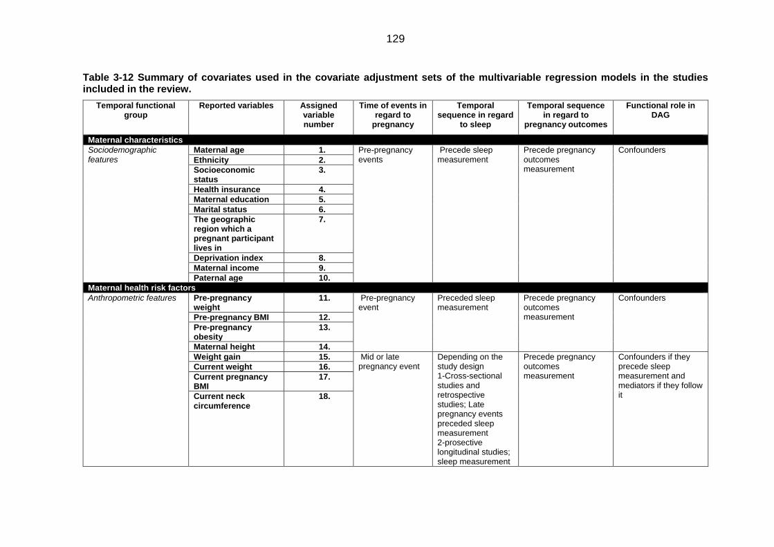
129
Table 3-12 Summary of covariates used in the covariate adjustment sets of the multivariable regression models in the studies included in the review.
Temporal functional group
Reported variables Assigned variable number
Time of events in regard to
pregnancy
Temporal sequence in regard
to sleep
Temporal sequence in regard to
pregnancy outcomes
Functional role in DAG
Maternal characteristics
Sociodemographic features
Maternal age 1. Pre-pregnancy events
Precede sleep measurement
Precede pregnancy outcomes measurement
Confounders
Ethnicity 2.
Socioeconomic status
3.
Health insurance 4.
Maternal education 5.
Marital status 6.
The geographic region which a pregnant participant lives in
7.
Deprivation index 8.
Maternal income 9.
Paternal age 10.
Maternal health risk factors
Anthropometric features Pre-pregnancy weight
11. Pre-pregnancy event
Preceded sleep measurement
Precede pregnancy outcomes measurement
Confounders
Pre-pregnancy BMI 12.
Pre-pregnancy obesity
13.
Maternal height 14.
Weight gain 15. Mid or late pregnancy event
Depending on the study design 1-Cross-sectional studies and retrospective studies; Late pregnancy events preceded sleep measurement 2-prosective longitudinal studies; sleep measurement
Precede pregnancy outcomes measurement
Confounders if they precede sleep measurement and mediators if they follow it
Current weight 16.
Current pregnancy BMI
17.
Current neck circumference
18.

130
Temporal functional group
Reported variables Assigned variable number
Time of events in regard to
pregnancy
Temporal sequence in regard
to sleep
Temporal sequence in regard to
pregnancy outcomes
Functional role in DAG
preceded late events
Chronic maternal diseases
Chronic hypertension
19. Pre-pregnancy or early pregnancy events
Precede sleep measurement
Precede pregnancy outcomes measurement
Confounders
Diabetes mellitus 20.
Anaemia 21.
Coronary heart disease
22.
Hyperlipidaemia 23.
Pregnancy related maternal complications
Pre-eclampsia 24. Mid or late pregnancy events
Depending on the study design 1-Cross-sectional studies and retrospective studies; Late pregnancy events preceded sleep measurement 2-prosective longitudinal studies; sleep measurement preceded late events
Depending on the timing of the outcome 1-Might precede the outcome if the outcome was late pregnancy event or after birth event 2- Might precede or follow the outcome if the outcome was mid pregnancy event
Confounders if they preceded sleep measurement and mediators if they follow it
Gestational diabetes 25.
Gestational hypertension
26.
Psychological disorders Pre-existing Depression
27. Pre-pregnancy or early pregnancy
Precede sleep Precede the outcome Confounders
Maternal behavioural risks
Smoking 28. Pre-pregnancy, early, mid or late pregnancy event
Might precede or follow sleep
Precede the outcome Confounders or mediators depending on their measurement time with regard to sleep
Alcohol 29.
Vitamin supplement during pregnancy
30.
Maternal obstetric history
Previous obstetric History Parity 31. Pre-pregnancy event
Preceded sleep measurement
Precede the outcome Confounders
Gravidity 32.
Prior preterm delivery
33. Pre-pregnancy event
Preceded sleep measurement
Precede the outcome Confounders
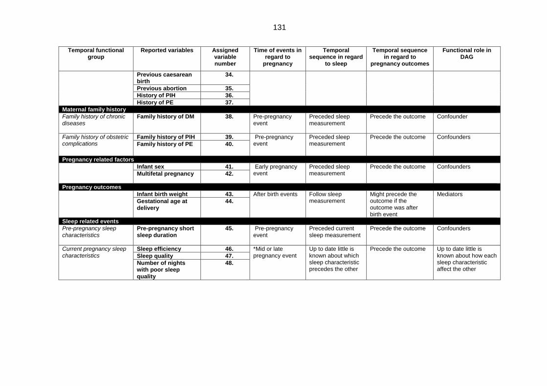
131
Temporal functional group
Reported variables Assigned variable number
Time of events in regard to
pregnancy
Temporal sequence in regard
to sleep
Temporal sequence in regard to
pregnancy outcomes
Functional role in DAG
Previous caesarean birth
34.
Previous abortion 35.
History of PIH 36.
History of PE 37.
Maternal family history
Family history of chronic diseases
Family history of DM 38. Pre-pregnancy event
Preceded sleep measurement
Precede the outcome Confounder
Family history of obstetric complications
Family history of PIH 39. Pre-pregnancy event
Preceded sleep measurement
Precede the outcome Confounders
Family history of PE
40.
Pregnancy related factors
Infant sex 41. Early pregnancy event
Preceded sleep measurement
Precede the outcome Confounders
Multifetal pregnancy 42.
Pregnancy outcomes
Infant birth weight 43. After birth events Follow sleep measurement
Might precede the outcome if the outcome was after birth event
Mediators
Gestational age at delivery
44.
Sleep related events
Pre-pregnancy sleep characteristics
Pre-pregnancy short sleep duration
45. Pre-pregnancy event
Preceded current sleep measurement
Precede the outcome Confounders
Current pregnancy sleep characteristics
Sleep efficiency 46. *Mid or late pregnancy event
Up to date little is known about which sleep characteristic precedes the other
Precede the outcome Up to date little is known about how each sleep characteristic affect the other
Sleep quality 47.
Number of nights with poor sleep quality
48.

132
Figure 3-4 Directed acyclic graph showing the temporal positions of each of the covariates included in the covariate adjustment sets of the regression models in the studies included in the review – including those using retrospective longitudinal study designs or prospective study designs with sleep measurements recorded later in pregnancy.

133
Figure 3-5 Directed acyclic graph showing the temporal positions of each of the covariates included in the covariate adjustment sets of the regression models in the studies included in the review – including those using in the prospective study designs with sleep measurements recorded earlier in pregnancy.
3.3.3 The association between sleep characteristics and pregnancy
outcomes
When considering the direction of any associations observed between
unfavourable sleep events and the risk of poor pregnancy outcomes, it was found
that, with the exception of three adjusted models, all of the unfavourable sleep
events (as described in Tables 3-13 to 3-18) examined in each of the unadjusted
and adjusted models increased the risk of all of the poor pregnancy outcomes
examined (as described in Table 3-10). In the first of the models that constituted
exceptions to this rule, OSA was found to be associated with a lower the risk of
PIH (adjusted Log OR= 0.9; CI=0.30 to 2.04; Table 3-13). The second model found
that an inverse association between short sleep duration and SGA (adjusted
OR=0.90; CI=0.40 to 1.80; Table 3-14). However, both of these models included

134
covariates that were judged to be mediators in their covariate adjustment sets.
Meanwhile, the third and final model examined the association between sleep
duration (as a continuous variable) and hyperglycemia and found an inverse
relationship though without considering the possibility that this might have resulted
from an imbalanced U-shaped relationship (where an increased odds of
hyperglycaemia might have been caused by short or long duration sleep; adjusted
OR= 0.2; 0.1 to 0.8; Table 3-14).
In regard to the magnitude of the associations observed between unfavourable
sleep events and pregnancy outcomes, it was found that this tended to vary
primarily as a result of the following factors:
I. The type of unfavourable sleep events - it being evident that SDB-related
sleep characteristics symptoms had the strongest associations with poor
pregnancy outcomes, regardless of the poor pregnancy outcomes involved
(Table 3-13).
II. The type of pregnancy outcomes – it being evident that late pregnancy
maternal events (i.e. GDM, PE and PIH) had the strongest associations with
unfavourable sleep characteristics regardless of the specific unfavourable
sleep events involved.
III. The categorisation of the unfavourable sleep characteristic used – this was
clearly evident when sleep duration was examined as a continuous variable.
Ignoring the possibility of a U-shaped relationship between sleep duration
and pregnancy outcomes appeared to reverse the direction of any
association between sleep duration and pregnancy outcomes (Table 3-15)
IV. The gestational age at which sleep was measured – it being evident sleep
measurements recorded earlier or later in pregnancy affected the strength
of any association between sleep and pregnancy outcomes, though without
affecting the direction of these associations. For instance O'Brien et al.
(2013) reported a far stronger association between snoring which
developed (and was measured) during the 3rd trimester and PIH (adjusted
OR=2.36; CI=1.48 to 3.77; Table 3-13) compared to snoring that developed
prior to the 3rd trimester (adjusted OR= 1.72; CI= 0.80 to 3.71; Table 3-13).
V. The choice of covariates included in the covariate adjustment sets used – it
being evident that including covariates likely to operate as mediators within
the covariate adjustment sets altered the direction of association between
OSA and PIH as well as that between SSD and SGA, whilst only affecting
the magnitude of the associations in the remainder of the inappropriately
adjusted models.

135
A detailed summary of the ORs extracted from the studies included in the review,
together with lists of the covariates included in these studies covariate adjustment
sets are listed in Table 3-13 through to Table 3-18.
Considering the number of pregnancy outcomes examined, it was clear that only
11 separate maternal/perinatal and neonatal outcomes have thus far been
examined by studies examining the relationship between sleep and pregnancy
outcomes. Furthermore, 3 of these have only been examined by a single study
each and few of the remainder have been studied with much consistency in either
the definition or categorisation of the variables examined, or in the study designs
adopted or the gestational age at which the sleep exposure variables were
measured.
At the same time, a total of (only) 8 separate/distinct sleep characteristics have
thus far been examined by such studies; and three of these characteristics have
only been examined, to-date, by a single study each; whilst for the others there
was, once more, little evidence of consistency in the definition, categorisation,
measurement tool/point or covariate adjustment sets used.
By far the most attention has been paid to maternal/perinatal characteristics than
to neonatal characteristics; and to snoring, OSA and (to a lesser extent) sleep
duration. Yet many of the studies failed to present either unadjusted and/or
adjusted coefficient estimates (which, together with the lack of consistency in terms
of methods, further reduces the scope for meta-analysis). Much of what is known
about the relationship between sleep and pregnancy outcomes is therefore based
on very little evidence (for most sleep characteristics and most pregnancy
outcomes), and appears to be sensitive to difference in sampling, measurement,
categorisation and analysis.

136
Table 3-13 Summary of adjusted and unadjusted ORs of studies that examined the relationship between SDB symptoms and poor pregnancy outcomes.
Stu
dy
de
sig
n
Refe
ren
ce
SD
B c
om
po
ne
nt
Tri
meste
r
Sam
ple
siz
e
Un
ad
jus
ted
OR
95%
co
nfi
da
nte
inte
rval
Ad
jus
ted
OR
95%
co
nfi
da
nte
in
terv
al
Temporal functional groups (TFG)
Ad
jus
ted
vari
ab
les
Nu
mb
er
of
TF
Gs
Nu
mb
er
of
med
iato
rs
Nu
mb
er
of
co
nfo
un
de
rs
Small for gestational age
Retrospective longitudinal study
(Bourjeily et al., 2010)
Snoring 3rd 1000 1.90 0.80 to 4.30 - - Un-adjusted 0 0 0
(Franklin et al., 2000)
Snoring 3rd 502 - - 2.03 1.01 to 4.10 1,11, 28 3 0 3
Prospective longitudinal
(Howe et al., 2015)
Snoring Not
specified 633 - - 1.20 0.60 to 2.40
1,2, 3,12,16,18, 27, 31, 41, 44
6 1 5
(Ko et al., 2013) OSA Not
specified 276 - - 2.56 0.56 to 11.68 1,32, 44, 3 0 3
(O'Brien et al., 2013)
OSA 3rd 1673 1.60 0.70 to 3.90 - - Un-adjusted 0 0 0
Low birth weight
Retrospective longitudinal study
(Chen et al., 2012)
OSA Not
specified 4786 2.16 1.61 to 2.90 1.72 1.42 to 2.40
1, 5, 6, 7,10,21, 22, 28,32,41
7 1 6
Prospective longitudinal
(Sharma et al., 2016)
Habitual snoring
Not specified
273 - - 2.70 1.00 to 7.20 Not reported Not
reported Not
reported Not
reported
Apgar score
Retrospective longitudinal (Bourjeily et al.,
2010)
OSA and 1 min Apgar
3rd 1000 - - 1.90 1.00 to 3.40 1,28,42 3 0 3
OSA and 5 min Apgar
3rd - - 3.70 1.10 to 11.90 1,28,42 3 0 3
(Chen et al., 2012)
OSA and 5 min Apgar
Not specified
4786 - - 10.11 3.45 to 29.67 1 1 0 1
Prospective longitudinal
(Sharma et al., 2016)
Habitual snoring and 5 min Apgar
Not specified
273 1.30 0.40 to 4.10 Not reported Not
reported Not
reported Not
reported
NICU ddmissiom
Prospective longitudinal
Louis et al., 2012)
OSA Not
specified 171 3.39 1.23 to 9.32 3.96 1.63 to 9.63 1, 2, 12 2 0 2
Still birth
Case control
(Stacey et al., 2011)
Snoring Not
specified 467 - - 1.12 0.75 to 1.67 1, 2,3, 12,28, 31 3 1 3
(Gordon et al., 2015)
Snoring 3rd 295 1.20 0.70 to 1.90 - - Un-adjusted 0 0 0

137
Stu
dy
de
sig
n
Refe
ren
ce
SD
B c
om
po
ne
nt
Tri
meste
r
Sam
ple
siz
e
Un
ad
jus
ted
OR
95%
co
nfi
da
nte
inte
rval
Ad
jus
ted
OR
95%
co
nfi
da
nte
in
terv
al
Temporal functional groups (TFG)
Ad
jus
ted
vari
ab
les
Nu
mb
er
of
TF
Gs
Nu
mb
er
of
med
iato
rs
Nu
mb
er
of
co
nfo
un
de
rs
(Gordon et al., 2015)
Apnea 3rd 295 1.20 0.60 to 2.10 1.60 0.65 to 4.20 Not reported Not
reported Not
reported Not
reported
Preterm delivery
Retrospective longitudinal
(Bourjeily et al., 2010)
OSA 3rd 1000 - - 1.90 1.10 to 3.30 1,28,42 3 0 3
(Louis et al., 2010)
OSA Not
specified 171 - - 2.60 1.00 to 6.60
1,2,4,13, 19,20,28, 33
5 2 3
Prospective longitudinal
(Louis et al., 2012)
OSA Not
specified 175 1.07 0.37 to 3.08 0.63 0.18 to 2.24 1, 2, 12 2 0 2
(Na-rungsri et al., 2016)
OSA 2nd 959 2.10 1.32 to 3.36 2.00 1.20 to 3.34 1, 12, 28,33,35 4 1 3
Caesarean delivery
Retrospective longitudinal
(Bourjeily et al., 2010)
Snoring 3rd 1000 2.10 1.40 to 3.20 2.10 1.40 to 3.20 28, 42, 43 3 0 3
OSA 3rd 1000 1.8 0.80 to 4.10 1.80 0.80 to 4.20 28, 42, 43 3 0 3
(Chen et al., 2012)
OSA Not
specified 4786 1.73 1.48 to 2.02 1.74 1.48 to 2.04
1, 5, 6, 7,10, 21, 22, 28, 32, 41
7 1 6
Prospective longitudinal
(Ko et al., 2013) OSA Not
specified 276 - - 1.53 0.79 to 2.96 1,32, 44, 3 0 3
(Louis et al., 2012)
OSA
Not specified
175 3.86 1.6 to 9.33 3.04 1.14 to 8.10 1, 2, 12 2 0 2
(O'Brien et al., 2013)
Chronic snoring
1st and 2nd
1673 2.00 1.33 to 3.04 2.25 1.22 to 4.18 5, 24, 25, 34,43 4 0 4
Pregnancy
onset snoring
3rd 1673 1.43 1.06 to 1.92 1.70 1.13 to 2.57 5, 24, 25, 34,43 4 0 4
(Sharma et al.,
2016) Habitual snoring
Not specified
273 - - 2.90 1.00 to 8.20 Not reported Not
reported Not
reported Not
reported
GDM
Prospective longitudinal
(Qiu et al., 2010)
Snoring Not
specified 1290 - - 6.91 2.87 to 16.60 1, 2, 12 2 0 2
(Reutrakul et al., 2011)
Snoring 2nd 169 - - 3.40 1.30 to 8.80 12 1 0 1
OSA 2nd 3.00 1.20 to 7.40 - - Un-adjusted 0 0 0
(O’Brien et al., 2012)
Pregnancy onset
snoring 3rd 1719 1.29 0.96 to1.74 - - Un-adjusted 0 0 0
Chronic snoring
1st and 2nd
1.67 1.10 to 2.52 - - Un-adjusted 0 0 0

138
Stu
dy
de
sig
n
Refe
ren
ce
SD
B c
om
po
ne
nt
Tri
meste
r
Sam
ple
siz
e
Un
ad
jus
ted
OR
95%
co
nfi
da
nte
inte
rval
Ad
jus
ted
OR
95%
co
nfi
da
nte
in
terv
al
Temporal functional groups (TFG)
Ad
jus
ted
vari
ab
les
Nu
mb
er
of
TF
Gs
Nu
mb
er
of
med
iato
rs
Nu
mb
er
of
co
nfo
un
de
rs
Prospective longitudinal
(Facco et al., 2010)
Snoring 2nd 189 4.90 1.30 to 18.10
6.90 1.40 to 33.90 1, 2,45 2 0 2
Retrospective longitudinal
(Bourjeily et al., 2010)
Snoring 3rd 1000 2.70 1.70 to 4.30 2.10 1.30 to 3.40 28, 42,43 3 0 3
Retrospective longitudinal
Bourjeily et al., 2010)
OSA 3rd 1000 2.60 1.30 to 5.50 2.00 0.90 to 4.30 3, 16, 28 3 0 3
Chen et al., 2012)
OSA
Not specified
4786 1.45 0.99 to 2.11 1.63 1.07 to 2.48 1, 5, 6, 7,10, 21,
22, 28, 32,41 7 1 6
Case control (Reutrakul et
al., 2013) OSA
Late 2nd to 3rd
45 - - 6.60 1.15 to 37.96 12 1 0 1
Pre-eclampsia
Retrospective longitudinal
(Franklin et al, 2000)
Snoring 3rd 502 - - 2.18 0.50 to 2.68 1, 12, 16, 42 4 0 4
(Owusu et al, 2013)
Snoring 3rd 234 - - 3.50 1.40 to 8.50 1, 31, 44 3 0 3
Prospective longitudinal
(O'Brien et al, 2012)
Pregnancy onset
snoring 3rd 1719 1.71 1.20 to 2.44 1.59 1.06 to 2.37
1, 2, 5, 12, 15, 28, 32, 36, 37,
40 7 2 5
Chronic snoring
1st to 2nd 1719 - - 1.12 0.58 to 2.14 1, 2, 5, 12, 15, 28, 32, 36, 37,
40 7 2 5
(Sharma et al., 2016)
Habitual snoring
Not specified
273 - - 1.50 0.50 to 4.90 Not reported Not
reported Not
reported Not
reported
(Ko et al, 2013) OSA Not
specified 276 - - 1.99 0.23 to 17.70 1,32, 44, 3 0 3
(Louis et al, 2012)
OSA Not
specified 175 3.60 1.47 to 8.84 3.54 1.26 to 9.92 1, 2, 12 2 0 2
(Ugur et al., 2012)
OSA Not
specified 465 - - 12.40 4.90 to 13.90 32, 44 2 0 2
Retrospective longitudinal
(Chen et al, 2010)
OSA Not
specified 4786 1.60 1.45 to 6.55 3.08 2.16 to 11.26
1, 5,6, 7,10, 21, 22, 28, 32, 41
7 1 6
Gestational hypertension
Retrospective longitudinal (Bourjeily et al.,
2010)
Snoring 3rd 1000 4.00 2.40 to 6.50 2.30 1.40 to 4.00 1,12, 19, 24, 25,
28, 42 6 1 5
OSA 3rd 1000 1.30 0.60 to 3.20 0.90 0.30 to 2.40 1,12, 19, 24, 25,
28, 42 6 1 5

139
Stu
dy
de
sig
n
Refe
ren
ce
SD
B c
om
po
ne
nt
Tri
meste
r
Sam
ple
siz
e
Un
ad
jus
ted
OR
95%
co
nfi
da
nte
inte
rval
Ad
jus
ted
OR
95%
co
nfi
da
nte
in
terv
al
Temporal functional groups (TFG)
Ad
jus
ted
vari
ab
les
Nu
mb
er
of
TF
Gs
Nu
mb
er
of
med
iato
rs
Nu
mb
er
of
co
nfo
un
de
rs
Retrospective longitudinal
(Franklin et al., 2000)
Snoring 3rd 502 - - 2.03 1.01 to 4.10 1,16, 28 3 0 3
(Perez-Chada et al., 2007)
Snoring Not
specified 456 - - 1.82 1.16 to 2.84
1, 12, 15, 18, 28, 29
4 2 2
OSA Not
specified 456 - - 3.15 1.50 to 6.61
1, 12, 15, 18, 28, 29
4 2 2
Prospective longitudinal
(O'Brien et al, 2012)
Pregnancy onset
snoring 3rd 1719 2.57 1.69 to 3.53 2.36 1.48 to 3.77
1, 2, 5, 12, 15, 28, 32, 36, 37,
40 7 2 5
Chronic snoring
1st 1719 - - 1.72 0.80 to 3.71 1, 2, 5, 12, 15, 28, 32, 36, 37,
40 7 2 5
(Sharma et al., 2016)
Habitual snoring
Not specified
273 - - 2.90 1.00 to 8.20 Not reported Not
reported Not
reported Not
reported
Retrospective longitudinal
(Reid et al., 2011)
OSA 3rd 219 8.30 2.10 to 33.40
- - Un-adjusted 0 0 0
(Chen et al,
2010) OSA
Not specified
4786 1.45 0.99 to 2.11 1.63 1.07 to 2.48 1, 3, 4, 12, 19, 20, 31, 32, 33,
44 8 0 8
Case control (Champagne et al., 2009)
OSA >20
weeks 50 5.60
1.40 to 23.20
7.50 3.50 to 16.20 1, 12, 31, 44 4 0 4

140
Table 3-14 Summary of adjusted and unadjusted ORs of studies that examined the relationship between sleep duration and poor pregnancy outcomes
Stu
dy
des
ign
Refe
ren
ce
Pre
gn
an
cy
ou
tco
mes
Sle
ep
du
rati
on
ris
k g
rou
p
Sa
mp
le s
ize
Tri
me
ste
r
Un
ad
jus
ted
OR
95
% C
I
Ad
jus
ted
OR
95
% C
I
Functional temporal groups (TFG)
Ad
jus
ted
va
ria
ble
s
Nu
mb
er
of
TF
Gs
Nu
mb
er
of
me
dia
tors
Nu
mb
er
of
co
nfo
un
de
rs
Neonatal outcomes
Case control
Stacey et al. (2011)
Still birth >8
hr/night 467 > 2nd 1.83 1.14 to 2.94 - - Unadjusted 0 0 0
Prospective longitudinal
Abeysena et al. (2009)
Small for gestational age
≤ 8 hr/night
690 1st 1.14 0.75 to 1.74 - - Unadjusted 0 0 0
Small for gestational age
≤ 8 hr/night
690 2nd 1.50 0.96 to 2.34 - - Unadjusted 0 0 0
Small for gestational age
≤ 8 hr/night
690 3rd 1.23 0.77 to 1.89 - - Unadjusted 0 0 0
(Howe et al., 2015)
Small for gestational age
<6 hr/night
633 3rd - - 0.90 0.40 to 1.80 1, 2, 5, 14, 15, 17, 19, 31, 38, 42
7 1 6
Small for gestational age
9 hr/night
633 3rd - - 1.60 0.80 to 32.00 1, 2, 5, 14, 15, 17, 19, 31, 38, 42
7 1 6
(Abeysena et al., 2010)
Low birth weight
> 8 hr/night
885 Not
specified 1.87 1.16 to 3.02 - - Unadjusted 0 0 0
Case control
Samaraweera and
Abeysena (2010)
Miscarriage >8
hr/night 734
Not specified
- - 3.80 1.01 to 14.30 44 1 0 1
Maternal outcomes
Prospective longitudinal Qiu et al.
(2010)
GDM <4
hr/night 1290 1st - - 5.50 1.31 to 23.69 1, 2, 12 2 0 2
GDM >9
hr/night 1290 1st - - 4.18 0.94 to 18.60 1, 2, 12 2 0 2
Facco et al.
(2010) GDM <7
hr/night 189
Not specified
2.6 1.3 to 5.5 2.40 1.10 to 5.30 1, 2, 12, 20 3 0 3

141
Stu
dy
des
ign
Refe
ren
ce
Pre
gn
an
cy
ou
tco
mes
Sle
ep
du
rati
on
ris
k g
rou
p
Sa
mp
le s
ize
Tri
me
ste
r
Un
ad
jus
ted
OR
95
% C
I
Ad
jus
ted
OR
95
% C
I
Functional temporal groups (TFG)
Ad
jus
ted
va
ria
ble
s
Nu
mb
er
of
TF
Gs
Nu
mb
er
of
me
dia
tors
Nu
mb
er
of
co
nfo
un
de
rs
Prospective longitudinal
Reutrakul et al. (2011)
GDM <7 hr/night
169 Not
specified 2.40 1.00 to 5.90 - - Unadjusted 0 0 0
Wang et al, 2017)
GDM <7 hr/night
12,506 Not
specified 1.36 0.87 to 2.14 1.12 0.69 to 1.81 1 1 0 1
GDM ≥ 9 hr/night
12,506 Not
specified 1.21
1.013 to 1.42
1.29 1.09 to
1.52 1 1 0 1
Herring et al., (2014)
Hyperglycaemia None 63 2nd 0.30 0.10 to 0.80 0.20 0.10 to 0.80 1, 2, 5, 12, 14, 19, 31,
38, 42. 7 0 7
Lee and Gay (2004)
Caesarean delivery
< 6 hr/night
63 2nd - - 4.54 1.36 to 15.21 43 1 0 1
Caesarean delivery
6 to 6.9 hr/night
131 3rd - - 3.67 1.33 to 10.18 43 1 0 1
Williams et al. (2010)
Preeclampsia ≤ 6
hr/night 1272 1st 2.64 0.82 to 8.56 2.36 0.72 to 7.72 1, 12, 31 3 0 1
Case control
Kajeepeta et al., (2014)
Preterm delivery
< 6 hr/night
959 1st and
2nd 1.55
1.11 to 2.16
1.56 1.11 to 2.19 1, 11, 30 3 0 3
Preterm delivery
≥ 9 hr/night
959 1st and
2nd 1.33 0.94 to 1.87 1.34 1.04 to 2.16 1, 11, 30 3 1 2

142
Table 3-15 Summary of adjusted and unadjusted ORs of studies that examined the relationship between sleep quality and poor pregnancy outcomes.
Stu
dy
des
ign
Refe
ren
ce
Pre
gn
an
cy
ou
tco
mes
Tri
me
ste
r
Sa
mp
le s
ize
Un
ad
jus
ted
OR
95
% C
I
Ad
jus
ted
OR
95
% C
I
Ad
jus
tme
nt
Temporal functional group
Nu
mb
er
of
TF
Gs
Nu
mb
er
of
me
dia
tors
Nu
mb
er
of
co
nfo
un
de
rs
Maternal outcomes
Prospective longitudinal
(Lee and Gay, 2004)
Caesarean delivery
3rd 131 - - 4.30 1.05 to16.93 12 1 0 1
(Reutrakul et al., 2011)a
Preterm delivery 2nd 169
1.20 1.00 to 1.30 - - Unadjusted 0 0 0
(Okun et al., 2011)
Preterm delivery 3rd 166 1.10 1.03 to 1.18 1.25 1.04 to1.5 9 1 0 1
(Stinson and Lee, 2003)
Preterm delivery 2nd 359 2.36 1.09 to 5.07 - - Unadjusted 0 0 0
(Wang et al., 2017)
GDM and moderately poor
quality
Not specified
12,506 1.62 1.20 to 2.17 1.19 1.01 to 1.41 1, 2, 5, 14, 15, 17,
19, 31, 38, 42 7 1 6
Neonatal outcomes
Prospective longitudinal
(Howe et al., 2015)
Small for gestational age
3rd trimester
633 - - 1.00 0.40 to 2.00 1, 2, 8, 17, 27, 28,
31, 41, 45, 48 7 1 6
Small for gestational age
3rd trimester
633 - - 1.10 0.50 to 2.70 1, 2, 8, 17, 27, 28,
31, 41, 45, 48 7 1 6

143
Table 3-16 Summary of adjusted and unadjusted ORs of studies that examined the relationship between sleep disturbance, latency and poor pregnancy outcomes.
Stu
dy
des
ign
Refe
ren
ce
Pre
gn
an
cy
ou
tco
mes
an
d
sle
ep
Tri
me
ste
r
Sa
mp
le s
ize
Un
ad
jus
ted
OR
95
% C
I
Ad
jus
ted
OR
95
% C
I
Temporal functional group (TFG)
Ad
jus
ted
va
ria
ble
s
Nu
mb
er
of
TF
Gs
Nu
mb
er
of
co
nfo
un
de
rs
Nu
mb
er
of
me
dia
tors
Maternal outcomes
Prospective longitudinal
(Lee and Gay, 2004)
Caesarean delivery and disturbance
3rd 131 - - 5.19 1.77 to 15.18
43 1 0 1
Neonatal outcomes
Case control (Stacey et al.,
2011) Still birth and disturbance 3rd 467 - - 2.42
1.46 to 4.00
1, 2, 3, 12, 28
4 0 4
Prospective longitudinal
(Strange et al., 2009)
Preterm delivery and latency 2nd 220 - - 1.04 1.01 to
1.07 33, 46, 47,48,
2 0 2
Table 3-17 Summary of adjusted and unadjusted ORs of studies that examined the relationship between daytime sleepiness and poor pregnancy outcomes.
Stu
dy
des
ign
Refe
ren
ce
Pre
gn
an
cy
ou
tco
mes
Tri
me
ste
r
Sa
mp
le s
ize
Un
ad
jus
ted
OR
95
% C
I
Ad
jus
ted
OR
95
% C
I
Temporal functional group (TFG)
Ad
jus
ted
va
ria
ble
s
Nu
mb
er
of
FT
Gs
Nu
mb
er
of
me
dia
tors
Nu
mb
er
of
co
nfo
un
de
rs
Maternal outcomes
Retrospective longitudinal
(Bourjeily et al., 2013)
Elective caesarean section
Not specified
1000 1.80 1.03 to
3.11 1.76
0.99 to 3.10
42, 43 2 0 2
(Bourjeily et al., 2013)
Vaginal delivery Not
specified 1000 1.09
1.02 to 1.16
1.08 1.01 to
1.15 42, 43 2 0 2
Neonatal outcomes
Case control (Stacey et al.,
2011) Still birth 3rd 467 1.78
1.18 to 2.68
2.04 1.26 to
3.30 1, 12, 2, 31,
28, 3 4 0 4
Prospective longitudinal
(Reutrakul et al., 2011)
NICU admission 2nd 169 1.10 1.00
to1.30 - - Unadjusted 0 0 0

144
Table 3-18 Summary of adjusted and unadjusted ORs of studies that examined the relationship between sleep position and poor pregnancy outcomes.
Refe
ren
ce
Pre
gn
an
cy
ou
tco
mes
Tri
me
ste
r
Sam
ple
siz
e
Sle
ep
po
sit
ion
Un
ad
jus
ted
OR
95
% C
I
Ad
juste
d
OR
95
% C
I
Ad
jus
tmen
t
Temporal functional group
Nu
mb
er
of
TF
Gs
Nu
mb
er
of
me
dia
tors
Nu
mb
er
of
co
nfo
un
ders
Maternal outcomes
No studies were resulted
Neonatal outcomes
Case control
(Stacey et al., 2011)
Still birth 3rd 467 Supine 3.28 1.46 to
7.34 - - Unadjusted 0 0 0
3rd 467 Right side 1.88 1.14 to 3.10,
- - Unadjusted 0 0 0
3rd 467 Other
positions 2.00
1.20 to 3.33
- - Unadjusted 0 0 0
(Gordon et al., 2015)
Still birth 3rd 295 Supine 5.00 1.50 to
16.5 6.26
1.20 to 34
Not reported
Not reported
Not reported
Not reported
Retrospective longitudinal
(Owusu et al., 2013)
Still birth Not
specified 234 Supine - - 8.00
1.50 to 43.20
1, 31, 44 3 0 3
Low birth weight
234 Supine - - 2.00 1.20 to
3.33 1, 31, 44 3 0 3

145
3.3.4 Meta-analysis results
Because of the limited number of studies that examined similar exposure-outcome
pairs using similarly sound analytical techniques (Table 3-11) it was only possible
to generate just 4 sets of meta-analyses, each containing the results of three or
more comparable analytical models. These were those examining the relationships
between:
1- short sleep duration and GDM using adjusted models with covariate
adjustment sets that did not include likely mediators (3 models; Figure 3-6)
2- OSA and CS using adjusted models with covariate adjustment sets that did
not include likely mediators (3 models; Figure 3-7)
3- OSA and PE using adjusted models with covariate adjustment sets that did
not include likely mediators (3 models; Figure 3-8)
4- snoring and GDM using (only) un-adjusted models (3 models) or only
adjusted models with covariate adjustment sets that did not include any
likely mediators (4 models; Figure 3-9)
These meta-analyses confirmed that short sleep duration was associated with an
increased risk of GDM (summary ES= 2.07; CI= 1, 06 to 4.04; Figure 3-6). A very
similar association was observed between snoring and GDM in the meta-analysis
of unadjusted models (summary ES= 2.31; CI= 1.44 to 3.70; Figure 3-9a), although
this strengthened considerably when using models that had adjusted (only) for
covariates likely to have operated as potential confounders (summary ES= 3.72;
CI= 1.92 to 7.18; Figure 3-9b).
As for OSA, this was found to be associated with an increased risk of both CS and
PE. OSA was associated with an increased risk of CS of 1.87 (CI=1.18 to 2.95;
Figure 3-7) and an increased risk of PE of 5.73 (CI= 1.87 to 17.56; Figure 3-8) in
meta-analyses that only included models in which the covariate adjustment sets
contained only confounders (and no mediators).
In addition, it was also clear that there was substantial heterogeneity amongst the
models included in most of these meta-analyses (Figure 3-6, Figure 3-8, Figure
3-9 and Figure 3-10), the exception being in the meta-analysis examining the
relation between OSA and CS, in which heterogeneity was not detected (Figure
3-7). The heterogeneity between studies included in each of the former meta-
analysis was primarily due to differences in the study design (prospective vs
retrospective longitudinal), the studies’ inclusion and exclusion criteria (such as
multiple pregnancies, maternal health conditions/risk factors and the gestational
age at which participants were recruited), the measurement tool used to assess
the sleep characteristic of interest (be that objective vs subjective) and the referent

146
categories used for these sleep characteristics (short vs long duration or habitual
vs non habitual events).
Figure 3-6 Forest plot summarising the ORs of studies that examined the relationship between short sleep duration and GDM using adjusted models that did not include possible mediators

147
Figure 3-7 Forest plot summarising the ORs of studies that examined the relationship between OSA and caesarean delivery using adjusted models that did not have any possible mediators
Figure 3-8 Forest plot summarising the ORs of studies that examined the relationship between OSA and pre-eclampsia adjusted models that did not have any possible mediators
Overall (I-squared = 0.0%, p = 0.520)
(Ko et al., 2013)
ID
Study
(Louis et al., 2012)
(Bourjeily et al., 2010)
1.87 (1.18, 2.95)
1.53 (0.79, 2.96)
OR (95% CI)
3.04 (1.14, 8.10)
1.80 (0.80, 4.20)
100.00
47.88
Weight
%
21.73
30.38
1.87 (1.18, 2.95)
1.53 (0.79, 2.96)
OR (95% CI)
3.04 (1.14, 8.10)
1.80 (0.80, 4.20)
100.00
47.88
Weight
%
21.73
30.38
1.5 1 2 4 6 8 10

148
Figure 3-9 Forest plot summarising the ORs of studies that examined the relationship between snoring and GDM using un-adjusted (a) and adjusted models that had no mediators (b).
.

149
3.4 Discussion
3.4.1 Limitations
By far, the most serious limitations of the review described in the present chapter
were as follows:
First, the limited numbers of studies on (some) unfavourable sleep events and
(some) pregnancy outcomes. Unfortunately, as seen in Table 3-11 many of the
pregnancy outcomes have not yet been fully examined in relation to all of the
unfavourable sleep events examined. Indeed, since sleep is likely to be a
multifactorial, complex phenomenon, in order to understand its full effect on
pregnancy outcome this will require examining all measurable sleep characteristics
in relation to each of the outcomes of interest concerned.
Second, the extensive evidence of methodological heterogeneity in the studies
(and their models) observed/as extracted and summarised. The extent of this
heterogeneity amongst studies limited the number of models that could be
combined in subsequent meta-analyses, and required substantial care to be taken
to examine in great detail the range of different study designs used; the range of
exposures, outcomes and covariates measured; the range of different measures
used for each cognate exposure and outcome, the timing of such measurements,
and the treatment of such data (e.g. if and how categorical variables were derived
from the raw data); and the range of different analytical techniques and covariates
included in the covariate adjustment sets used by each analytical model.
In addition, this review was prone to a number of limitations that remain
commonplace for all such reviews, including:
I. The potential risk of not identifying or including all available studies due to
possible limitations in the search protocol or the search inclusion criteria
used;
II. The inappropriate classification of covariates acting as confounders vs.
mediators during the design and/or analysis of each primary study;
III. The limited external validity (generalizability) of results due to limitations in
the study’s exclusion/inclusion criteria, its setting and/or design;
IV. The insufficient information available about the quality of the data used and
how (if at all) missing data were treated in any of the primary studies
included.
V. The small sample sizes of many of the primary studies (as well as the lack
of power/sample size calculations to assess the impact of this) which would

150
increase the chance of type II errors (finding the absence of an association
between sleep and poor pregnancy outcomes when an association exists)
and decrease the power of any analyses as well as the precision of their
estimates.
VI. The absence of adequate adjustment for multiple testing which might
increase the chance of type I errors (finding, in this instance, the presence
of an association between sleep and poor pregnancy outcomes when no
such association actually exists).
VII. The possibility of publication bias, especially considering that only papers
describing at least one statistically significant finding were found in the
review’s search of the literature, even though their designs/methods
suffered at least one of the limitations mentioned earlier.
In the forest plots summarized below (Figure 3-10), studies with smaller samples
of participants commonly had effect sizes/coefficient estimates situated towards
the right hand extremes of the graphs, as their ORs tended to be much larger than
the null with 95% CIs that did not include 1.0 (i.e., indicative of a ‘statistically
significant’ finding). In contrast, most of the studies with larger sample sizes tended
to report at least one regression model in which the effect size/coefficient estimate
did not achieve formal ‘statistical significance’ and were aggregated closer to (or
either side of) the null, 1.0. This is likely to reflect the fact that studies with smaller
sample sizes usually have less statistical power and a higher chance of type II
errors than studies with larger sample sizes, particularly in the absence of a priori
sample size/power calculations used to inform sampling. Hence, one would
expected to find more of the studies with smaller sample sizes reporting findings
that did not achieve formal ‘statistical significance’, and fewer such studies with
larger sample sizes. However, in this review, approximately two-thirds of the
articles examined (n= 17) had relatively modest sample sizes (of ≤500 participants)
yet reported ‘statistically significant’ estimates with large ORs. As sample sizes
increased, fewer of the reported models achieved formal ‘statistical significance’ –
which constitutes prima facie evidence of publication bias.
Whilst the failure to access unpublished studies (or all published studies) and to
include foreign language studies may have contributed to the appearance
publication bias (Dickersin, 1990); approximately 63% of the articles included had
been published in English-speaking countries, and only three articles included in
the search were written in a non-English language. The latter suggests that
restricting the search to English language articles had, at most, only a very minor
influence on the magnitude of potential publication bias, since only a small number

151
of published studies on this topic had been performed in non-English-speaking
countries (and fewer still had been published in a language other than English).
With regard to the generalisability of the results (whether from each specific study
or from the meta-analyses undertaken), limited information was generally available
about the socioeconomic status of many of the studies’ participants, and most of
the studies applied exclusion criteria (including for social characteristics, such as
English language proficiency) that are likely to have limited the external
validity/generalizability of their findings. This is because, for example, language
proficiency might reflect both ethnicity and/or socioeconomic status, so that
excluding participants with limited English language proficiency might inevitably
lead to selection bias. Furthermore, it is notable that more than two-thirds of the
published studies took place in the USA, and that none had been conducted in the
UK. The disproportionate geographical distribution of studies might therefore limit
the wider, international generalisability of the results reviewed due simply to the
influence of environmental factors on sleep events and pregnancy outcomes that
differ internationally.
Finally, in the vast majority of the studies reviewed insufficient information was
provided concerning current and pre-pregnancy medical health conditions of the
participants included. In some studies participants with specific health conditions,
such as gestational diabetes (GDM), were excluded from the sample. Some such
conditions, not least GDM, affect a substantial proportion of pregnant women and
are displaying a gradual increase over time (e.g. GDM affects about 2–7% of
pregnant women and has increased substantially over the last 20 years; Lawrence
et al., 2008, Ben‐Haroush et al., 2004). Excluding women with such conditions from
any given study sample means that it may not be appropriate to apply the research
findings of that study to them, especially when (as is the case for conditions such
as GDM) the conditions themselves increase the risk of both unfavorable sleep
events and poor pregnancy outcomes (albeit depending upon the time at which
sleep and the conditions concerned are measured). One would therefore expect to
find potentially different results amongst currently published studies and pregnant
women experiencing such conditions, and knowledge in this regard remains
scarce.

152
Figure 3-10 Forest plot summarising the un-adjusted (a) and adjusted (b) ORs of the regression models reported in the included references
.

153
3.4.2 Key findings
The aim of this review was to evaluate the findings of published studies examining
the association between sleep and pregnancy outcomes. It found that only a very
limited number of studies had examined the association between unfavourable
sleep events and pregnancy outcomes; and that not all unfavourable sleep
characteristics and pregnancy outcomes had received an equal level of attention
in the literature. Indeed, some sleep events (i.e. latency, disturbance and daytime
sleepiness) and some pregnancy outcomes (i.e. Apgar score, birth weight and late
maternal pregnancy events) have not been examined at all to-date. Nonetheless,
despite the relatively few sleep characteristics and pregnancy outcomes examined,
there was still evidence of a general tendency towards positive associations
between unfavorable sleep and poor pregnancy outcomes in which unfavorable
sleep characteristics were associated with an increased risk of poor pregnancy
outcomes. However, much of this evidence had multiple methodological flaws, and
there was some evidence of publication bias. These methodological flaws
decreased the certainty offered by the current evidence available, and undermined
the level of precision available – so that the summarized findings cannot be
interpreted with substantial confidence and should be applied with circumspection
and a degree of scepticism.
The review also found that the magnitude of the increased risk of poor pregnancy
outcomes associated with unfavourable sleep characteristics varied according to
the pregnancy outcome and/or sleep characteristic examined. This also varied in
relation to a range of specific study design criteria, including: the design of the
primary studies; the inclusion and exclusion criteria used in the recruitment of study
participants; the gestational age at which sleep was measured; the choice of
covariates included in any covariate adjustment sets; the appropriateness of any
adjustment achieved; and the use of various reference points for what were
considered ‘normal’ sleep characteristics as well as variation in the measurement
tools used – all of which appeared to have affected the magnitude of the estimated
risks, causing either an increase or decrease in the estimated ORs, and (in a few
instances) appeared to have reversed the direction of the association observed.
Although our assumptions regarding the possible impact(s) of these aspects of
study design and analysis on the magnitude and direction of the estimated ORs
might be true, the lack of the precisely estimated ORs made it difficult to assess or
confirm with any degree of confidence whether these aspects were actually the
reasons why substantial differences were evident amongst the estimated results.
154
However, considering these aspects of study design, data measurement and
analysis, and their likely impact on the estimation of any casual pathway between
sleep and pregnancy outcomes (while also considering the potential bidirectional
nature of any relationship between sleep and the majority of covariates included in
the regression models examined in this review), it is sensible to consider each of
the following issues (each of which were discussed previously in the methodology
chapter [Chapter 2, Section 2.4, page 60] when the original ‘hypothesized’ DAG
was first presented and explained):
I. First, the importance of considering each study’s design when specifying
the relationship between sleep and pregnancy outcomes (particularly
whether the design is retrospective or prospective).
II. Second, the importance of the temporal sequence of events, since this can
be crucial when specifying the direction of any causal arc when dealing with
potentially bidirectional relationships.
III. Third, the importance of reporting/knowing the time (i.e. the gestational age)
at which sleep and other covariates were measured (to help avoid the
inclusion of mediators in the covariate adjustment sets used).
IV. Fourth, the importance of carefully considering the timing of measurements
when repeated measurements of sleep and/or other covariates are
available (again, to help avoid the inclusion of mediators in the covariate
adjustment sets used).
In addition to the covariates included in the hypothesized DAG described earlier in
the present thesis, this was further elaborated by the inclusion of variables that had
been adjusted for by one or more of the studies included in this chapter’s review–
each of which were carefully categorised as: sociodemographic indicators;
behavioral risk indicators; current (and/or previous) maternal health indicators;
current (and/or previous) obstetric-related variables; psychological indicators; and
fetal health indicators. However, some of these (additional) variables were also
considered likely to have had bidirectional relationships with sleep, and as such
might have been likely to behave as mediators (rather than confounders) according
to their position in the DAG.
3.4.3 Conclusion
In conclusion, this review of previous studies examining the association between
(a range of) sleep (characteristics) and (a range of) pregnancy outcomes found
some evidence that such associations do indeed exist. However, this evidence is
limited in scope since not all measurable sleep characteristic and not all available
pregnancy outcomes were examined by these studies; while sleep was never

155
‘holistically’ defined (an important consideration given its complex nature and
substantial variability between each of the different trimesters of pregnancy).
Additionally, the evidence summarized and appraised in the present review is
highly variable in quality both in terms of data (quality) and the presence of a
number of potential biases (most importantly selection bias and confounding bias).
Finally, many of the evidence summarized herein came from studies that appear
severely underpowered.
Meanwhile, the possibility of publication bias may indicate that much of the
currently published evidence is prone to type I and type II error – not least because
the majority of published results are nominally ‘statistically significant’ even though
many of the studies involved appear underpowered. As such, it seems likely that
the currently available/published evidence overestimates the strength of the
relationship between sleep and pregnancy outcomes.
3.4.4 Recommendations
Further research is needed in this area with: greater consistency in the
measurement of sleep and pregnancy outcomes (particularly with regard to the
reference point used, the measurement tool used, and the gestational age when
sleep was measured); more evidence from less commonly examined sleep
characteristics and pregnancy outcomes (particularly sleep latency and
macrosomia, respectively); and more robust study designs and analytical
techniques (particularly as regards sampling, power estimation and adjustment for
confounding). There is also scope for extending the research undertaken to include
more participants with additional risks of poor pregnancy outcome (such as those
with gestational diabetes or those at risk of diabetes), who are often excluded from
existing study populations. Improving the conceptualization of sleep (beyond the
definition and measurement of its many disparate, yet inherently related,
characteristics and components), would also be worth pursuing (using, for
example, latent class analysis).

156
Chapter 4 Sleep Patterns in the United Kingdom Population: a
latent class analysis of the UKHLS
4.1 Introduction
Sleep is a complex phenomenon which, though amenable to objective study (in
most detail using polysomnography), also has important experiential
characteristics that are cognitive and subjective (Carskadon and Dement, 2017).
While there remains substantial debate on how best to measure sleep, and how
best to distinguish the specific components and characteristics these
measurements generate, it remains clear that: different measurements offer
different perspectives on these different components and characteristics (Kryger
et al, 2011, Van Den Berg et al, 2008); some components and characteristics are
associated with sociodemographic, behavioural and clinical factors (Arber et al,
2009) . These associations include evidence that sleep may cause, and be caused
by, a variety of disease states – evidence that has led to a resurgence of interest
in the role of sleep in the aetiology of disease, and the potential role that sleep-
enhancing interventions might play in disease prevention and treatment
(Cappuccio et al, 2010, Alvarez and Ayas, 2004). However, despite growing
acceptance that sleep plays a significant role in memory consolidation and mental
health, and mounting evidence that sleep is likely to be both a cause and a
consequence of poor somatic health, there remain few non-pharmacological
interventions (beyond ‘sleep hygiene’ advice) that are amenable to
experimentation, and limited experimental evidence that ‘enhancing’ sleep may
have therapeutic benefits in non-clinical populations (Reid et al, 2006, Montgomery
and Dennis, 2004). For this reason, much of the current evidence base linking
variation in sleep to variation in health is based on studies adopting observational
designs and dependent upon observational data (Cappuccio et al, 2010, Alvarez
and Ayas, 2004). These studies face a theoretical and methodological challenge
that is common to many analyses of observational data where there are multiple
measureable characteristics of a single phenomenon, yet little firm knowledge of
the functional causal relationships between these. In the absence of such
knowledge it is difficult to apply recent developments in causal path modelling to
design statistical models capable of confidently adjusting for confounders
(variables causing both the exposure and outcome of interest) while avoiding
inappropriate adjustment for mediators (variables forming part of the causal path
between the exposure and the outcome).

157
As summarised in the previous chapter, in the literature sleep has tended to be
examined as a potential determinant of pregnancy outcomes using one single
sleep characteristic at a time. Occasionally, multiple characteristics have been
included in a single analytical model, though without a proper understanding of
how these characteristics might be functionally or causally related to a more
‘holistic’ concept of sleep per se, or how these characteristics might interact with
one another. Indeed, it seems most likely that sleep is a complex phenomenon,
best described in quantitative terms as a latent variable, measured using multiple
indicators rather than any single characteristic.
Notwithstanding this ‘holistic’ view of sleep, it is important to recognise that what
might constitute ‘normal’ sleep is likely to vary dramatically between individuals –
such that what is considered ‘normal’ for one individual may be experienced as
‘abnormal’ for another. Furthermore, because sleep varies from one night to the
next, it is likely to be challenging to measure sleep using rigid cut-off points for
‘normal’ vs. ‘abnormal’ sleep without incurring substantial measurement error.
The present chapter aimed to address these issues by applying Latent Class
Analysis (LCA) to a large contemporary dataset with data on a range of different
sleep characteristics, and thereby establish whether these characteristics might
(when considered together, in a more ‘holistic’ fashion) reflect any hitherto hidden
sleep ‘patterns’. The present Chapter also aimed to assess the temporal stability
of any LCA-identified sleep patterns (using data on sleep characteristics collected
twice from the same individuals) and to assess whether any such patterns are
associated with sociodemographic and/or clinical variables. As such the present
Chapter aimed not only to establish whether sleep patterns might be identified from
data on multiple sleep characteristics, but also whether these patterns display
temporal stability and appear sensitive to sociodemographic, behavioural and
clinical characteristics thought to influence (and/or to be influenced by) sleep.
4.2 Methods
4.2.1 Data source
The data used in the present chapter were taken from Waves 1 and 4 of the UK
Household Longitudinal Study (UKHLS) which was accessed through the UK Data
Archive website during 2014 -2016 (Chapter 2, Section 2.2.1, page 17). These data
were originally gathered by the National Centre for Social Research (NatCen) and
the Central Survey Unit (CSU) under the direction of the UK Longitudinal
Studies Centre (University of Essex. Institute for Social and Economic Research
and NatCen Social Research, 2015).

158
The UKHLS is a large ongoing study covering most of the UK’s geographical area,
and has a sampling design that aims to generate participants who are
representative of the UK population as a whole. The study includes questionnaire
items covering many of the most commonly studied sleep components (i.e. as
evident in the literature on sleep reviewed earlier in this thesis), as well as items
generating data on sociodemographic, behavioural and health-related clinical
features which permit further examination of their relationships with sleep using
latent class analysis (see: Chapter 2, Section 2.1.2.1, page 47).
4.2.2 Study design
4.2.2.1 ‘Temporal stability’ study
A cross-sectional design was initially used to generate the latent class sleep
models for both Waves 1 and 4 separately, first using participants who had
participated in both Waves. Thereafter, a longitudinal study design was used to
compare the stability of the resulting latent sleep models from each Waves (i.e. at
Wave 1 vs. Wave 4) over time.
4.2.2.2 ‘Correlates of latent sleep classes’ study
After assessing the stability of sleep models over time, a third sample of
participants (comprising all those offering responses to the survey’s questionnaire
sleep items; and based on the very first time each participant answered these items
[be that in Wave 1 or in Wave 4]) was analysed to identify latent sleep classes from
the largest possible sample of participants available. For assessing the
sociodemographic, behavioural and clinical correlates of latent sleep classes,
relevant data were extracted from responses given to items in the same wave as
that providing the sleep data used. (i.e. the sociodemographic/behavioural/clinical
data generated from the questionnaire in which participants first gave responses
to the sleep items).
4.2.3 Participants
As sleep data were only available from the questionnaires used in Waves 1 and 4
of the UKHLS, only participants providing responses to from these two UKHLS
Waves were eligible for inclusion in the present chapter.
Male participants as well as female participants were included in the present
chapter’s analyses to identify the latent sleep patterns amongst the UK population,
while analyses of their relationship(s) with pregnancy outcomes necessarily
include only (pregnant) women. This two-stage process was considered necessary
for the following reasons;

159
First, the aim was to discover all possible, stable sleep patterns amongst UKHLS
participants, and since women might share similar pattern with men we aimed to
maximize the number of participants involved.
Second, since the aim was then to describe the distribution of sleep in women as
compared to men, subsequent analyses were then conducted to establish which
patterns were more/less commonly associated with female participants.
Finally, the aim of these (gender-disaggregated) analyses was to examine whether
pregnant women’s sleep patterns differed in comparison to those of the general
population (i.e. male and female), since the literature contained claims that
pregnant women’s sleep was substantively less ‘favourable’ than the population as
a whole (claims that therefore required conducting latent class analyses not only
in pregnant women, but also amongst female participants separately and male and
female participants combined).
4.2.3.1 Temporal stability study
Male and female participants who participated in both Waves 1 and 4 of the UKHLS
and had complete sets of sleep data were included in the the sub-studies that
examined the stability of the latent class analysis approach over time when using
the UKHLS sleep module.
4.2.3.2 ‘Correlates of latent sleep classes study’
Male and female participants who participated in Wave 1 and/or Wave 4 and had
complete sets of sleep data were included in the latent class analysis to generate
the UK population sleep clusters .
4.2.4 Measurements
4.2.4.1 Sleep variables
To generate the sleep clusters in the temporal stability and correlates of sleep
classes studies, all seven sleep variables generated by items in the UKHLS sleep
module were used: sleep duration, latency, sleep disturbances due to snoring or
coughing, use of medication to help with sleep, next-day sleepiness, sleep
disturbance, and perceived sleep quality.
4.2.4.2 Coding of sleep variables
The sleep variables, which include latency, disturbance, snoring and/or coughing,
usage of medication and next-day sleepiness, were re-categorized using fewer
categories (3 ordinal categories) to make it easier to visualise more distinguished
patterns of variations between the generated clusters when conducting the latent
analysis (Table 4-1). The following classification was carried when categorising the

160
variables; absent, non-habitual (< 3 events a week) and habitual (≥ 3 times a
week), as it was the classification most often used in the literature and the
classification of insomnia symptoms used by the DSMVI (Amarican Psychiatric
Association, 2013). Sleep duration was categorised into four categories, using
similar to the Pittsburgh Sleep Quality Index (PSQI; Buysse et al, 1989) scoring
categories (Table 4-1; the sleep questionnaire most commonly used by sleep
researchers). This categorisation was chosen to facilitate comparison of any sleep
patterns identified in the present chapter with those described in the literature.
Table 4-1 The seven items in the Understanding Society Sleep Questionnaire, together with the original response categories and the categories adopted to facilitate comparison with studies using the PSQI.
Sleep questions Original responses Responses after reducing the numbers of categories
Q1: “How many hours of actual sleep did you usually get at night during the last month? Note: This may be different than the actual number of hours you spent in bed”.
Reported in hours and minutes Reference: ≥7 hours
Short: ≥6 and <7 hours Restricted: ≥5 and <6 hours Severely restricted: <5 hours
Q2: During the past month, how often have you had trouble sleeping because you “Cannot get to sleep within 30 minutes”?
1. Not during the past month 2. Less than once a week 3. Once or twice a week 4. Three or more times a week 5. More than once most nights
1. Not during the past month (1) 2. less than three times a week
(2&3) 3. Three or more times a week
(4&5)
Q3: During the past month, how often have you had trouble sleeping because you “Wake up in the middle of the night or early in the morning”?
1. Not during the past month 2. Less than once a week 3. Once or twice a week 4. Three or more times a week 5. More than once most nights
1. Not during the past month (1) 2. less than three times a week
(2&3) 3. Three or more times a week
(4&5)
Q4: During the past month, how often have you had trouble sleeping because you “Cough or snore loudly”?
1. Not during the past month 2. Less than once a week 3. Once or twice a week 4. Three or more times a week 5. More than once most nights
1. Not during the past month (1) 2. less than three times a week
(2&3) 3. Three or more times a week
(4&5)
Q5: During the past month, how often have you taken medicine (prescribed or “over the counter”) to help you sleep?
1. Not during the past month 2. Less than once a week 3. Once or twice a week 4. Three or more times a week
1. Not during the past month (1) 2. less than three times a week
(2&3) 3. Three or more times a week (4)
Q6: During the past month, how often have you had trouble staying awake while driving, eating meals, or engaging in social activity?
1. Not during the past month 2. Less than once a week 3. Once or twice a week 4. Three or more times a week
1. Not during the past month (1) 2. less than three times a week
(2&3) 3. Three or more times a week (4)
Q7: During the past month, how would you rate your sleep quality overall?
1. Very good 2. Fairly good 3. Fairly bad 4. Very bad
1. Good (1&2) 2. Bad (3&4)

161
4.2.4.3 The coding of sleep variables included in the exploratory
regression analyses
When running the regression analyses to evaluate the association between each
of the seven self-reported sleep characteristics and each of the sociodemographic,
and health characteristics, all of the sleep variables were re-categorised as binary
variables. The rationale for using binary variables was to permit comparison of the
logistic odd ratios generated for analyses of each sleep characteristic with those
generated for analyses of any/each LCA-derived sleep cluster.
Sleep duration was categorized as ≥7 hours and < 7 hours, while sleep latency,
disturbance, snoring and/or coughing, next-day sleepiness and sleep medication
was categorised as ‘ever versus never’. Sleep quality was categorised as
very/fairly good vs. fairly/very bad.
Sociodemographic features (i.e. age, gender, current employment status,
household composition and highest educational qualification achieved) were used
to study the associations between each of the seven sleep characteristics and
each/any sleep cluster. Data on each of the sociodemographic variables used were
extracted from the same wave as that providing the self-reported sleep data. Most
of the sociodemographic variables were re-categorised to simplify those with large
numbers of response categories, thereby ensuring that there were likely to be
sufficient numbers of participants in each of the reduced categories to permit robust
analysis.
A full description of how each of the sociodemographic variables were categorised
(before and after re-categorisation) is available in the appendices. A brief summary
is provided below:
I. Age was re-categorised into: ≤19 years, 20-39years, 40-59 years and ≥60
years.
II. Education was re-categorised into: ‘A’ level or above vs. GCSE level or
‘other’
III. Occupation was categorised into: employed, unemployed, sick or disabled,
in training/education, and retired
IV. Household structure was categorised into: Single without children, Single
with children, Couple without children, and Couple with children
4.2.4.4 Health indicators
Three indicators were chosen to provide measures of participant health, including
the physical and mental components of the eight items of the SF12v (a shorter
version of the SF36v developed by Quality Metric Incorporate; Quality Metric Inc.,

162
2007). These were used to subjectively evaluate each participant’s well-being and
functional health, including the first item of the SF12v (which provides a general
subjective evaluation of an individual’s overall health). The physical and mental
components of the SF12v were originally rated from 0 to 100, where the higher the
score, the ‘healthier’ the participant. The components were re-categorised into
three equal categories (i.e. 66, <66 and ≥ 32, <32) using ‘norm scoring’ (i.e. based
on the mean [M=50] and standard deviation [SD=16]; see Table 8-12). Likewise,
the general health variable was re-categorised into a binary variable: ‘excellent to
good’ and ‘fair to poor’. For further detail with regard to the SF12v questionnaire
please refer to the appendices (see Chapter 8, Section 8.3.1, page 314).
4.2.5 Ethical considerations
Ethical approval for the main survey of the UKHLS was obtained from the Ethics
Committee of the University of Essex on 6 July 2007 for Wave 1, and on 17
December 2010 for Wave 4 (Gundi, 2016).
4.3 Analysis
4.3.1 Descriptive analysis
4.3.1.1 Missing data
The following responses were recorded as missing: ‘I do not know’, ‘proxy’,
‘refused’ and ‘inapplicable’. The patterns of missing data observed suggested that
where data for one variable was missing, data for many/most of the other variables
were also missing. In these instances case-wise deletion (i.e. excluding
participants with missing data on any of the variables of interest) was applied.
In this way, cases/participants with missing sleep data were excluded from the
latent class analyses used to identify/generate ‘sleep clusters’. At the same time,
cases with missing sociodemographic data (age, gender, education, household
composition, employment) and/or missing health data (i.e. SF12v mental and
physical components, general health) were also excluded case-wise, prior to
conducting the regression analyses.
4.3.1.2 Participants characteristics
Frequencies and percentages were used to describe the distribution of the seven
sleep characteristics and each of the sociodemographic and health variables
amongst participants included in the analyses conducted in the present chapter.

163
4.3.2 Latent class analyses (LCA)
In the LCA the seven sleep variables were used as indictors of a complex latent
structure that was envisaged as having multiple categories (or ‘clusters’) within
which participants could be placed/classified. These classifications were based on
the principal of identifying participants who shared common patterns in their
responses to the sleep questions, and calculating the probability of each participant
being classified within each sleep cluster (Lazarsfeld and Henry, 1968, Goodman,
1974)
A latent class analysis was used to generate sleep clusters for both the temporal
stability and correlates of sleep classes studies. First, exploratory analyses were
conducted to generate models with a range of different numbers of clusters. Each
of the information criteria (i.e. BIC and AIC) statistics as well as measurement of
entropy statistics (i.e. R2 and estimation error) were used to compare different
latent models with differing numbers of clusters. In each case, the lower the
information criteria and the higher the R2 statistic the more robust the model was
considered to be, after considering the number of parameters included (since this
penalises the statistics; Vermunt and Magidson, 2005).
Latent Gold 4.5 software (Statistical Innovations Inc., 2009) was used to generate
the latent sleep clusters. It calculated the posterior probability of a participant being
a member of each cluster, and it then assigned each individual to the cluster with
the highest probability using the maximum likelihood (Vermunt and Magidson,
2005).
4.3.3 Regression analysis
For participants with complete sleep, sociodemographic and health indicator data
who also participated in Wave 1 and/or Wave 4, logistic regression analysis was
used to examine the association between each of the socio-demographic
characteristics, the health indicators and: the seven sleep variables; or the sleep
clusters assigned to participants generated using LCA.
After generating the latent sleep clusters using Latent Gold these were later
transferred to STATA-v13 software (StataCorp., 2013) as multinomial variables
before separating the categories into 6 binary variables with ‘yes’ or ‘no’ coding. At
this stage the multinomial regression was not considered ideal for the following
reasons:
1- The multinomial regression estimated the risk of several categories relative
to a single referent category yet, at this stage, it was not clear which
category should be chosen as the referent.

164
2- The multinomial regression approach would not estimate the risk for
participants classified within any given referent category, and this was
suboptimal given the intention was to estimate the risk for each category.
3- By coding the latent sleep variable that had six categories into six binary
variables with six different referents, it would be possible to understand the
risk relationship of each category by estimating their ORs and comparing
these with the OR of each sleep characteristic. This approach was intended
to assist in deciding which reference point might be used when running the
regression models in the next two chapters using the latent sleep variable.
The minimal sufficient adjustment sets in these regression models were specified
using a directed cyclic graph (DAG) - a graphical tool in which the relation between
the variables of interest are presented using unidirectional arrows that symbolise
the direction of potential causal effects between variables. It was generated
using open source software DAGitty (Textor et al., 2017).
4.4 Results
As illustrated in Figure 4-1, the total number of participants who participated in both
Waves 1 and 4 and who had complete sleep data in both waves (and thus were
included in the temporal stability study) was n=19,442. In contrast, the number of
participants who participated in either Waves 1 and/or 4 and had complete sleep
data (and were therefore in the correlates of sleep classes study) was n=45,141.

165
Figure 4-1 Flow chart of participants who participated in Waves 1 and/or 4 of the UKHLS and were involved in the temporal stability study and/or the correlates of sleep classes study.
4.4.1 Results of the descriptive analysis
4.4.1.1 Missing data
4.4.1.1.1 Mechanism of missing data
In Wave 1, the majority of missing data was secondary to a ‘failure to collect data’
(i.e. data missing or unattainable from proxy respondents). Indeed, only 19 of the
participants who were contacted refused to answer the sleep questions, the
majority of these being female (n=15), who did not appear to belong to any specific
age, employment or household composition group. Indeed, their education was
equivalent to GCSE or other in 11 out of 15 (see Table 4-2).
Likewise, the majority of missing data in Wave 4 was due to an inability to contact
participants (i.e. proxy, missing). Only seven participants refused to answer any of
the sleep questions. These were mostly males (n=5) who, again, did not appear to
belong to any specific age, education, employment or household composition
group.

166
Elsewhere, the majority of the ‘I do not know’ responses were recorded under the
‘snoring or coughing’ sleep item. These participants were primarily female (n=280)
and tended to be aged 70 or older (n=129). In addition, the majority of these also
had missing data on many of their sociodemographic characteristics.
Based on Table 4-2 and Table 4-3, it can be observed that where data on any one
sleep item were missing, then the data for other sleep items also tended to be
missing.
4.4.1.1.2 Characteristics of missing data
The distribution of missing data amongst each of the sociodemographic
characteristics was comparable to the distribution of participants with incomplete
sleep data (Table 4-4). Indeed, the distribution of missing data did not appear to
be dependent on particular sociodemographic features or clustered amongst
groups with specific characteristics.

167
Table 4-2 Known mechanisms underlying the (non)reporting of missing data for sleep items in Wave 1 of the UKHLS.
Wave 1
Missing Proxy Refused Inapplicable I don't know Total number
Frequency Percent Frequency Percent Frequency Percent Frequency Percent Frequency Percent
Duration 9,339 74.00 3,262 25.85 19 0.15 0 0.00 0 0.00 12,620 Latency 10,631 76.52 3,262 23.48 0 0.00 0 0.00 0 0.00 13,893 Disturbance 9,968 75.34 3,262 24.66 0 0.00 0 0.00 0 0.00 13,230 Snoring 13,735 80.81 3,262 19.19 0 0.00 0 0.00 0 0.00 16,997 Sleepiness 8,007 71.05 3,262 28.95 0 0.00 0 0.00 0 0.00 11,269 Medication 7,953 70.91 3,262 29.09 0 0.00 0 0.00 0 0.00 11,215 Quality 7,511 69.72 3,262 30.28 0 0.00 0 0.00 0 0.00 10,773
Total number 15,877 82.87 3,262 17.03 19 0.10 0 0.00 0 0.00 19,158
Table 4-3 Known mechanisms underlying the (non)reporting of missing data for sleep items in Wave 4 of the UKHLS.
Wave 4
Missing Proxy Refused Inapplicable I don't know Total number
Frequency Percent Frequency Percent Frequency Percent Frequency Percent Frequency Percent
Duration 15 0.37 3,940 98.01 2 0.05 0 0.00 65 1.62 4,020 Latency 14 0.35 3,940 98.99 2 0.05 0 0.00 24 0.60 3,980 Disturbance 14 0.35 3,940 99.14 2 0.05 0 0.00 18 0.45 3,974 Snoring 14 0.32 3,940 99.24 2 0.05 0 0.00 485 10.92 4,441 Sleepiness 13 0.33 3,940 99.24 1 0.03 0 0.00 17 0.43 3,970 Medication 14 0.35 3,940 99.42 2 0.05 0 0.00 7 0.18 3,963 Quality 14 0.35 3,940 98.80 2 0.05 0 0.00 32 0.80 3,988
Total number 15 0.33 3,940 86.25 7 0.15 0 0.00 606 13.27 4,568

168
Table 4-4 Sociodemographic characteristics of missing and complete sleep data in Waves 1 and 4 of the UKHLS.
Wave 1 (n=50,994) Wave 4 (n=47,157)
Complete sleep items Missing sleep items Complete sleep items Missing sleep items
Frequency Percent Frequency Percent Frequency Percent Frequency Percent
Gender Male 14,397 45.22 8,811 45.99 18,883 44.34 2,903 63.55 Female 17,439 54.78 10,347 54.01 23,706 55.66 1,665 36.45 Missing 0 0 0 0 0 0 0 0 Age ≤19 years 2,332 7.33 1,054 5.50 2,752 6.46 462 10.11 20-39years 11,806 37.08 5,666 29.58 12,255 28.78 1,669 36.54 40-59 years 11,083 34.81 6,313 32.95 15,253 35.81 1,468 32.14 ≥ 60 years 6,615 20.78 6,125 31.97 12,329 28.95 969 21.21 Missing 0 0 0 0 0 0 0 0 Education A level and above 18,256 57.34 7,826 40.85 23,297 54.70 2,205 48.27 GCSE level and others 13,569 42.62 11,251 58.73 18,520 43.49 2,157 47.22 Missing 11 0.03 81 0.42 772 1.81 206 4.51 Occupation Employed 18,600 58.42 8,881 46.36 23,257 54.61 2,648 57.97 Unemployed 4,080 12.82 2,990 15.61 4,661 10.94 471 10.31 Sick or disabled 1,226 3.85 1,132 5.91 1,726 4.05 238 5.21 Full time training or education 2,694 8.46 1,208 6.31 2,907 6.83 506 11.08 Retired 5,230 16.43 4,941 25.79 10,036 23.56 702 15.37 Missing 6 0.02 6 0.03 2 0 3 0.07 Household composition Single with children 2,938 9.23 1,857 9.69 3,434 8.06 334 7.31 Single without children 6,460 20.29 4,756 24.83 8,876 20.84 734 16.07 Couple with children 10,465 32.87 5,496 28.69 13,154 30.89 1,607 35.18 Couple without children 11,973 37.61 7,049 36.79 17,125 40.21 1,893 41.44 Missing 0 0 0 0 0 0 0 0 General health Excellent to good 25,987 81.63 13,916 72.64 33,758 79.26 3,526 77.19 Fair to poor 5,837 18.33 5,160 26.93 8,827 20.73 1,019 22.31 Missing 12 0.04 82 0.43 4 0.01 23 0.50 Physical wellbeing ≥ 66 167 0.52 95 0.50 163 0.38 4 0.09 <66 and ≥ 32 29,021 91.16 13,101 68.38 34,938 82.04 398 8.71 <32 2,560 8.04 2,456 12.82 3,712 8.72 94 2.06 Missing 88 0.28 3,506 18.30 3,776 8.87 4,072 89.14 Mental wellbeing ≥ 66 270 0.85 233 1.22 304 0.71 3 0.07
<66 and ≥ 32 29,716 93.34 14,117 73.69 35,980 84.48 444 9.72 <32 1,762 5.53 1,299 6.78 2,529 5.94 49 1.07 Missing 88 0.28 3,509 18.32 3,776 8.87 4,072 89.14

169
4.4.1.2 Sociodemographic features and health
A very similar distribution of sociodemographic and health characteristics was evident
within each of the samples selected for examination in the present chapter (i.e. Wave
1, Wave 4, temporal stability study and correlates of sleep classes study samples).
Overall, the ratio of male to female participants was very similar, whilst the majority of
participants were between 20 to 60 years of age, employed, had a partner, and were
in good mental and physical health (Table 4-5).
4.4.1.3 Sleep characteristics
The sleep data of participants included in the temporal stability study displayed a very
similar distribution as that from participants in Wave 1 or Wave 4 (see Table 4-
6).However, in the correlates of sleep classes study (i.e. which data generated from
the first response to the sleep questions was of key interest), there was an increase in
the rate of the following events: next-day sleepiness (44.2%), habitual snoring or
coughing (49.1%), habitual disturbance (62.1%), habitual latency (54.8%) and
restricted sleep duration (45.8%; Table 4-6)

170
Table 4-5 Sociodemographic features of UKHLS participants included in each of the samples used to generate latent sleep clusters.
Wave 1 Matched population
Wave 4 Matched population
Waves 1 and or 4 First time response
All Wave 1 participants
All Wave4 Participants
Frequency (n=19,442)
Percent (%=100)
Frequency (n=19,442)
Percent (%=100)
Frequency (n=45,121)
Percent (%=100)
Frequency (n=50,994)
Percent (%=100)
Frequency (n=47,157)
Percent (%=100)
Gender Male 8,479 43.61 8,479 43.61 20,456 45.32 23,208 45.51 21,786 46.20 Female 10,963 56.39 10,963 56.39 24,685 54.68 27,786 54.49 25,371 53.80 Missing 0 0 0 0 0 0 0 0 0 0 Age ≤19 years 1,047 5.39 309 1.59 4,514 10 2,450 4.80 3,214 6.82 20-39years 6,505 33.46 5,977 30.74 15,742 34.87 17,470 34.26 13,924 29.53 40-59 years 7,473 38.44 7,823 40.24 15,043 33.32 17,396 34.11 16,721 35.46 ≥ 60 years 4,417 22.72 5,333 27.43 9,842 21.80 12,740 24.98 13,298 28.20 Missing 0 0 0 0 0 0 0 0 0 0 Education A level and above 11,505 59.18 12,053 61.99 24,953 55.28 26,082 51.15 25,502 54.08 GCSE level and others 7,931 40.79 7,389 38.01 19,429 43.04 24,820 48.67 20,677 43.85 Missing 6 0.03 0 0 759 1.68 92 0.18 978 2.07 Occupation Employed 11,82 60.84 11,855 60.98 23,957 53.07 27,481 53.89 25,905 54.93 Unemployed 2,231 11.48 1,986 10.21 5,647 12.51 7,070 13.86 5,132 10.88 Sick or disabled 742 3.82 709 3.65 1,917 4.25 2,358 4.62 1,964 4.16 Full time training or education 1,154 5.94 585 3.01 4,835 10.71 3,902 7.65 3,413 7.24 Retired 3,483 17.91 4,307 22.15 8,782 19.45 10,171 19.95 10,738 22.77 Missing 3 0.02 0 0 3 0.01 12 0.02 5 0.01 Household condition 27,481 53.89 Single with children 1,623 8.35 1,425 7.33 4,153 9.20 4,795 9.40 3,768 7.99 Single without children 3,541 18.21 3,935 20.24 8,782 19.45 11,216 21.99 9,610 20.38 Couple with children 6,562 33.75 6,074 31.24 14,962 33.15 15,961 31.30 14,761 31.30 Couple without children 7,716 39.69 8,008 41.19 17,244 38.20 19,022 37.30 19,018 40.33 [;pl/.’k;0Missing 0 0 0 0 0 0 0 0 3,768 7.99 General health Excellent to good 15,983 82.21 15,856 81.56 36,807 81.54 39,903 78.25 37,284 79.06 Fair to poor 3,453 17.76 3,586 18.44 8,328 18.45 10,997 21.57 9,846 20.88 Missing 6 0.03 0 0 6 0.01 94 0.18 27 0.06 Physical wellbeing ≥ 66 92 0.47 78 0.40 216 0.48 262 0.51 167 0.35 <66 and ≥ 32 17,862 91.87 16,625 85.51 39,967 88.54 42,122 82.60 35,336 74.93 <32 1,488 7.65 2,739 14.09 3,558 7.88 5,016 9.84 3,806 8.07
Missing 0 0 0 0 1,400 3.1 3,594 7.05 7,848 16.64 Mental wellbeing ≥ 66 158 0.81 124 0.64 363 0.80 503 0.99 307 0.65 <66 and ≥ 32 18,221 93.72 16,985 87.36 40,818 90.42 43,833 85.96 36,424 77.24 <32 1,063 5.47 2,333 12.00 2,560 5.67 3,064 6.01 2,578 5.47 Missing 0 0 0 0 1,400 3.1 3,594 7.05 7,848 16.64

171
Table 4-6 Sleep characteristics of UKHLS participants included in the samples used to generate latent sleep clusters
Wave 1 Matched population
Wave 4 Matched population
Waves 1 and or 4 First time response
All Wave 1 participants
All Wave4 Participants
Frequency (n=19,442)
Percent (%=100)
Frequency (n=19,442)
Percent (%=100)
Frequency (n=45,121)
Percent (%=100)
Frequency (n=50,994)
Percent (%=100)
Frequency (n=47,157)
Percent (%=100)
Sleep duration ≥7 hours 12,628 64.95 11,210 57.66 16,561 36.69 24,671 48.38 24,861 52.72
≥ 6 and < 7 hours 5,230 26.90 5,133 26.40 5,764 12.77 8,987 17.62 11,014 23.36
≥ 5 hours and <6 hours 901 4.63 1,974 10.15 2,164 4.79 3,091 6.06 4,516 9.58
<5 hours 683 3.51 1,125 5.79 20,652 45.75 1,625 3.19 2,745 5.82 Missing 0 0 0 0 0 0 12,620 24.75 4,021 8.53 Sleep latency Never 8,263 42.50 9,326 47.97 11,549 25.58 15,228 29.86 20,426 43.31 Non-habitual (<3nights a week) 7,568 38.93 6,419 33.02 8,848 19.60 14,063 27.58 13,769 29.20 Habitual (≥ nights a week) 3,611 18.57 3,697 19.02 24,744 54.81 7,810 15.32 8,982 19.05 Missing 0 0 0 0 0 0 13,893 27.24 3,980 8.44 Sleep disturbance Never 4,426 22.77 6,136 31.56 8,194 18.15 8,538 16.74 13,921 29.52 Non-habitual (<3nights a week) 7,678 39.49 6,535 33.61 8,898 19.71 14,270 27.98 13,847 29.36
Habitual (≥ nights a week) 7,338 37.74 6,771 34.83 28,049 62.14 14,956 29.33 15,415 32.69 Missing 0 0 0 0 0 0 13,230 25.94 3,974 8.43 Snoring or coughing Never 12,384 63.70 15,540 79.93 18,976 42.04 21,378 41.92 34,185 72.49 Non-habitual (<3nights a week) 4,200 21.60 2,241 11.53 3,989 8.84 7,393 14.5 4,894 10.38
Habitual (≥ nights a week) 2,858 14.70 1,661 8.54 22,176 49.13 5,226 10.25 3,637 7.71
Missing 0 0 0 0 0 0 16,997 33.33 4,441 9.42 Next day sleepiness Never 16,434 84.53 17,397 89.48 22,249 49.29 33,469 65.63 38,394 81.42 Non-habitual (<3nights a week) 2,711 13.94 1,701 8.75 2,940 6.51 5,516 10.82 3,841 8.15 Habitual (≥ nights a week) 297 1.53 344 1.77 19,952 44.20 740 1.45 951 2.02 Missing 0 0 0 0 0 0 11,269 22.10 3,971 8.42 Usage of sleep medication Never 16,452 84.62 17,981 92.49 22,764 50.43 32,827 64.37 39,651 84.08 Non-habitual (<3nights a week) 1,369 7.04 723 3.72 1,400 3.10 3,149 6.18 1,603 3.40 Habitual (≥ nights a week) 1,621 8.34 738 3.80 20,977 46.47 3,803 7.46 1,940 4.11 Missing 0 0 0 0 0 0 11,215 21.99 3,963 8.40 Sleep quality Good 15,299 78.69 15,547 79.97 20,594 45.62 31,124 61.03 34,343 72.83 Poor 4,143 21.31 3,895 20.03 24,547 54.38 9,097 17.84 8,826 18.72 Missing 0 0 0 0 0 0 10,773 21.13 3,988 8.46

172
4.4.2 Results of generating the sleep clusters
4.4.2.1 Choosing the best-fit model
In the temporal stability study, the best fitting model included six clusters in data from
both Wave 1 and Wave 4. Both of these models were the simplest models, with the
lowest BIC, AIC and estimation error as well as the highest R2 (after accounting for
the number of parameters examined). Similarly, the models with six clusters were
chosen as the simplest models with the lowest BIC, AIC and estimation error as well
as the highest R2 (again, when considering the number of parameters used) in the
subsequent ‘correlates of sleep classes’ sub-study (see Appendix, Section 8.3.2, page
316).
It is important to note, however, that when binary coding was used for the seven sleep
indicators to generate the clusters (instead of the original categorisation), the temporal
stability of the sleep clusters over time was lost. This loss of stability was evident in
number of the differences in the patterns of sleep clusters that emerged between data
from Wave 1 and 4, despite the fact that the number of clusters remained the same
(see Appendix, Section 8.3.4, page 317).
4.4.2.2 Description of sleep patterns and clusters
In the temporal stability study, the best fitting models in both Waves (1 and 4) were
models containing six clusters, with a number of similarities in patterns therein. Three
clusters displayed essentially identical patterns (clusters 1, 3 and 6), whilst the
remaining three clusters differed in the severity of restriction of sleep duration and/or
the frequency of sleep latency. Inconsistencies in the contribution that sleep duration
made was observed in clusters 2 and 4. In cluster 2, the relevant sleep duration
changed from normal to short, while in cluster 4, the duration changed from short to
restricted (i.e. one-hour difference). Likewise, in cluster 2, the frequency of sleep
latency changed from non-habitual to habitual, while in cluster 5 this changed from
non-habitual to no event (i.e. a change of just one adjacent category; Table 4-7 and
Table 4-8).
Regardless of the stability of the six clusters between data generated in Wave 1 and
Wave 4, there was also some evidence that participants ‘moved’ between sleep
clusters from Wave 1 to Wave and 4 (i.e. their membership of sleep cluster changed
over time; Table 4-9). Most such movements involved participants who moved from
cluster 2 in Wave 1 to cluster 1 in Wave 4 (n=2,244, 58.4%), whilst the least number
of participants moved from cluster 3 in Wave 1 to cluster 2 in Wave 4 (n=61, 2%). The
most stable cluster was cluster 1, since 61% of participants who were members of this
cluster remained in that cluster in both Wave 1 and Wave 2. At the other extreme,

173
cluster 2 had the least stability, since only 296 (7.7%) of the participants in that cluster
remained therein.
In the correlates of sleep classes study, the best fitting model was the model that had
six clusters, as it was the simplest model with the lowest BIC (taking account of the
number of parameters examined (Table 4-10). These clusters were named on the
basis of the patterns observed there in, paying particular attention to the following
sleep items: sleep duration, subjective assessment of sleep quality and the most
dominant sleep-related event. In this way the six clusters were referred to as short bad
sleeper, long moderate sleeper, long good sleeper, disturbed bad sleeper, struggle-
to-sleep sleeper and snoring good sleeper. The majority of participants were in cluster
1 (n=19464, 43.1%), and the minority were in cluster 6 (n=1,591, 3.5%). Cluster 1 had
the highest prevalence of unfavourable sleep events, whilst cluster 3 had a complete
absence of unfavourable sleep events. Clusters 4 and 5 shared similar patterns of
unfavourable sleep events, except that cluster 5 had a poor level of sleep quality.
Cluster 6 included participants with habitual (i.e. frequently occurring) snoring and
habitual disturbances but with normal quality and duration. Cluster 2 contained
participants exhibiting non-habitual sleep disturbances in the absence of other sleep-
related events.
Table 4-7 Patterns of sleep clusters based on the latent class analysis for participants from Wave 1 who also participated in Wave 4 (n=19,442). The patterns described are based on the probabilities of the mean event within each cluster.
Cluster 1 Cluster 2 Cluster 3 Cluster 4 Cluster 5 Cluster 6
Duration Normal Normal Normal Short Short Short
0.846 0.604 0.788 0.421 0.462 0.447
Latency No event Non-
habitual
No event Habitual Non-
habitual
Non-
habitual
0.467 0.545 0.964 0.986 0.531 0.557
Snoring No event No event No event No event No event No event
0.708 0.483 0.904 0.404 0.538 0.616
Disturbance Non-
habitual
Habitual No event Habitual Habitual Non-
habitual
0.671 0.655 0.999 0.968 0.998 0.668
Sleepiness No event No event No event No event No event No event
0.904 0.858 0.929 0.676 0.728 0.671
Medication No event No event No event No event No event No event
0.905 0.826 0.911 0.643 0.783 0.797
Quality Good Good Good Bad Bad Bad
1.000 0.999 0.991 0.876 0.989 0.705

174
Table 4-8 Patterns of sleep clusters based on the latent class analysis for participants from Wave 4 who had previously participated in Wave 1 (n=19,442). The patterns described are based on the probabilities of the mean event within each cluster.
Cluster 1 Cluster 2 Cluster 3 Cluster 4 Cluster 5 Cluster 6
Duration Normal Short Normal Restricted Short Short
0.723 0.397 0.769 0.411 0.370 0.394
Latency No event Habitual No event Habitual No event Non-
habitual
0.473 0.923 0.988 0.942 0.719 0.553
Snoring No event No event No event No event No event No event
0.809 0.673 0.946 0.653 0.721 0.748
Disturbance Non-
habitual
Habitual No event Habitual Habitual Non-
habitual
0.524 0.992 0.999 0.959 0.997 0.524
Sleepiness No event No event No event No event No event No event
0.919 0.907 0.966 0.755 0.823 0.803
Medication No event No event No event No event No event No event
0.951 0.858 1.000 0.723 0.882 0.887
Quality Good Good Good Bad Bad Bad
1.000 0.600 0.991 0.998 0.604 0.575
Table 4-9 The distribution of participants amongst clusters in Waves 1 and 4 presented as percentages and frequencies.1
Wave 4
Wav
e 1
Cluster 1 Cluster 2 Cluster 3 Cluster 4 Cluster 5 Cluster 6 Total
Cluster 1 (n) 5,137 275 1,805 285 352 309 8,163
(%) 62.93 3.37 22.11 3.49 4.31 3.79 100.00
Cluster 2 (n) 2,244 296 509 305 329 157 3,840
(%) 58.44 7.71 13.26 7.94 8.57 4.09 100.00
Cluster 3 (n) 1,431 61 1,351 64 82 95 3,084
(%) 46.40 1.98 43.81 2.08 2.66 3.08 100.00
Cluster 4 (n) 528 228 111 801 209 177 2,054
(%) 25.71 11.10 5.40 39.00 10.18 8.62 100.00
Cluster 5 (n) 539 78 112 215 320 107 1,371
(%) 39.31 5.69 8.17 15.68 23.34 7.80 100.00
Cluster 6 (n) 416 45 119 115 76 159 930
(%) 44.73 4.84 12.80 12.37 8.17 17.10 100.00
Total (n) 10,295 983 4,007 1,785 1,368 1,004 19,442
(%) 52.95 5.06 20.61 9.18 7.04 5.16 100.00
1 Bold text indicates the percentages of participants who remained within their clusters between Wave
1 and 4.

175
Table 4-10 Patterns of sleep clusters based on the latent class analysis for participants from Wave 1and/or Wave 4 (n=45, 141). The patterns described are based on the probabilities of the mean event within each cluster.
Cluster1 Cluster 2 Cluster 3 Cluster 4 Cluster 5 Cluster 6
Cluster name Short Bad sleeper
Long Moderate sleeper
Long good
sleeper
Disturbed bad sleeper
Struggle to sleep-er
Snoring good
sleeper
Cluster size n (%)
19,464 (43.12)
13,343 (29.56)
3,186 (7.06)
5,186 (11.49)
2,371 (5.25)
1,591 (3.52)
Duration Severely restricted
Normal Normal Short Restricted Normal
0.9998 0.778 0.820 0.349 0.301 0.587
Latency Habitual No event No event
Non-habitual
Habitual Non-
habitual
0.9999 0.446 0.963 0.498 0.999 0.493
Coughing or snoring
Habitual No event No event No event No event Habitual
0.9999 0.751 0.981 0.722 0.557 0.229
Disturbance Habitual
Non-habitual
No event Habitual Habitual Habitual
1.000 0.503 0.999 0.530 0.981 0.709
Sleepiness Habitual No event No event No event No event No event
0.9998 0.906 0.960 0.776 0.738 0.643
Medication Habitual No event No event No event No event No event
0.9999 0.929 0.957 0.853 0.697 0.647
Quality Bad Good Good Bad Good Good
1.000 0.999 0.993 0.646 0.863 0.673
4.4.3 Results of the regression analysis
4.4.3.1 Adjustment for confounding
Based on the DAG presented in Figure 4-2, the following adjustments were applied
when conducting each of the linear regression models: age was adjusted for gender;
education was adjusted for age and gender; employment was adjusted for age, gender
and education; household structure was adjusted for gender, age, education and
employment; and mental and physical health were both adjusted for age, gender,
education, household structure and employment.

176
Figure 4-2 DAG representing the association between sleep, sociodemographic features and health indicators. The variables are represented by rectangles squares, and the direction of potential causal influence between variables are represented by unidirectional arrows.
4.4.3.2 The association between sociodemographic, health features and
sleep
In comparison to the six sleep patterns, the seven individual sleep characteristics
displayed far less variability in their associations with sociodemographic and health
features. (Table 4-11, Table 4-12, Table 4-13 and Table 4-14)
Female participants were more likely to display sleep latency, sleep disturbance and
poorer sleep quality, and to report using sleep-related medication than men. In
addition, female participants were far less likely to be associated with cluster 3 ‘good
long sleeper’ compared to men and this might in part reflect the effect of hormonal
differences and hormonal variability (i.e. during menstruation, menopause and
pregnancy as well as postpartum). In addition, older participants were less likely to
report sleep latency and daytime sleepiness than younger participants. Participants
who were older and female were significantly more likely to have particular sleep
patterns, such that: compared to those aged less than 20 years, people aged between
20–39 years tended to be found within cluster 1 (“short bad sleeper”), and those
between 40–69 years tended to be found in either cluster 1 or 6 (“snoring good
sleeper”); while participants who were older than 70 years had a six times higher odds
of being snorers with a good perceived sleep quality.
Participants with lower educational attainment were more likely to exhibit all of the
unfavourable sleep examined (with the exception of disturbance). Participants who
were unemployed also had a higher risk of experiencing unfavourable sleep events,

177
while participants with poor health indicators (i.e. unemployment due to sickness, a
lower score in the mental and physical component of the SF12V and poor reported
subjective health) were more likely to report unfavourable sleep events across all
seven individual sleep characteristics. These trends in the association between
individual sleep characteristics and health was noticeably absent when the association
between health and latent sleep clusters was examined. Instead, health displayed a
range of different relationships (positive and negative, strong and weak) with the six
sleep pattern clusters/classes.
Full-time trainees/students had the lowest risk of being associated with ostensibly
unfavourable sleep patterns compared to those who were employed or on leave. This
might in part be related to an age effect. Meanwhile, educational attainment was
associated with a range of different sleep pattern clusters: participants with
postgraduate qualifications had twice the odds of being in cluster 5 (“struggle-to-sleep-
er”) compared to those with a degree. Having no qualifications increased the risk of
being classified in cluster 6 (“snoring good sleeper”) as well as in cluster 5.
Household structure, in terms of presence of children or living as couples, had a range
of different associations with different sleep pattern clusters. For example, in
comparison to single participants without children, being single with children
decreased the risk of being associated with cluster 6 (“snorers, good sleepers”),
perhaps because snorers are usually not aware of their snoring unless informed by a
bed partner (i.e. acting as a witness). Being a couple without children significantly
decreased the odds of being in cluster 5 (“struggle-to-sleep-er”) – as such it was
associated with a lower odds of experiencing sleep latency, or disturbance or
protracted sleep duration. Perhaps caring for young children might cause some degree
of sleep disturbance as parents often awake to settle, change or feed their children if
these wake in the night. Living with others, either as couples or not, and with/without
children, decreased the odds of being associated with sleep patterns that had
unfavourable events (as compared with living alone). However, this finding should not
be mistaken with the likely effects of overcrowding or cohabitation with extended
families on the availability of sleeping space/accommodation as the latter had a higher
odds of being associated with bad sleep quality and shorter duration sleep (Fowler et
al., 2014).
4.4.3.2.1 Sociodemographic features and sleep
In regards to the seven sleep characteristics, when compared to participants younger
than 20 years of age, those who were older than 40 years of age had an odds of short
sleep duration that was three times higher (OR= 3.31, CI = 3.03, 3.61), while the odds
of disturbance (OR=2.30, CI=2.14, 2.47) and snoring (OR=2.75, CI=2.52, 3.00) were

178
both over twice as high. In participants older than 60 years of age, the odds of using
medication to help with sleep was two times higher (OR=2.52, CI=2.21, 2.88). Female
participants displayed a higher tendency towards unfavourable sleep events than
males, excluding snoring or coughing (OR=0.66, CI=0.64, 0.69) and short sleep
duration (OR=0.95, CI=0.913, 0.98) where females had a substantially and modestly
lower odds thereof, respectively. In general, participants with lower education
attainment had a modestly higher odds of unfavourable sleep events, except the odds
of disturbance, which was marginally lower amongst participants with lower
educational attainment (OR=0.95, CI=0.91, 0.99). Compared to employed individuals,
participants who were unemployed or undergoing training displayed a higher odds of
unfavourable sleep events. On the other hand, the odds of reporting poor sleep quality
(OR=0.90, CI=0.82, 0.99), short sleep (OR=0.72, CI=0.681, 0.76) and snoring or
coughing (OR=0.76, CI=0.70, 0.82) were all lower amongst participants who were
retired. The association between each of the categories of household structure and
the risk of unfavourable sleep events varied, but in general it appeared that: a those
participants living alone without any children had a higher odds of unfavourable sleep
events, except snoring or coughing. Having children increased these odds to OR=1.18
(CI=1.08, 1.29), having a partner increased the odds to OR=1.36 (CI=1.29, 1.45) and
having a partner plus children increased the odds to OR= 1.20 (CI=1.13, 1.28).
In regards to sleep clusters, female participants were more likely to be in clusters 1, 5
and 6 than males. The highest odds for females was to be in cluster 5 (OR =1.61,
CI=1.47, 1.31). Being older than 20 years of age increased the odds of being included
in clusters 1 and 5. The odds of being in cluster 1 was three times higher in the age
group 40-59 years (OR=3.07, CI=2.84, 3.32), two times higher in the age group 20 to
39 years (OR=2.14, CI=1.98, 2.31) and more than two times higher for the age group
older than 60 (OR=2.67, CI=2.46, 2.90).Lower education was associated with a higher
odds of being included in clusters 4, 5 and 6 with the highest odds being membership
of cluster 5 (OR=1.75, CI=1.60, 1.91).
The association between employment and cluster membership varied. Participants
who were enrolled in education or training programs had a higher odds of being in
cluster 2 (OR=1.35, CI=1.23, 1.48) and cluster 4 (OR=1.26, CI=1.11, 1.42).
Unemployed participants had a higher odds of being in cluster 5 (OR=1.86, CI=1.64,
2.11) and cluster 6 (OR=1.77, CI=1.52, 2.07). Similarly, more retired participants
tended to be in cluster 5 (OR=1.59, CI=1.30, 1.94) and cluster 6 (OR=1.53, CI=1.19,
1.97).
Compared to single participants without children, having children increased the odds
of being in cluster 1 by OR= 1.26 (1.16, 1.37). In addition, having a partner increased

179
the odds of being in cluster 1 by OR=1.13 (CI=1.07, 1.19) and being in cluster 3 by
OR=1.24 (CI=1.12, 1.38). In a very similar fashion, having a partner and children
increased the odds of being in cluster 1 by OR=1.31 (CI=1.24, 1.39).
4.4.3.2.2 Health indicators and sleep
Overall, participants with low scores for the mental and physical components of the
SF12v (i.e. total score < 32), and participants who reported a bad to poor level of
perceived general health, showed an elevated risk of developing unfavourable sleep
events. A low score on the SF12v physical component increased the odds of reporting
poor sleep quality by more than six times (OR=6.19, CI=5.67, 6.76) and by more than
two times for using sleep-related medication (OR=2.64, CI=2.41, 2.89) and reporting
next-day sleepiness (OR=2.40, CI=2.14, 2.70). A low score for the mental components
of the SF12v was also associated with an increase of three times the odds of reporting
poor sleep quality (OR=3.03, CI=2.77, 3.83) and daytime sleepiness (OR=3.07,
CI=2.77, 3.41), and of almost twofold for each the remaining sleep characteristics.
Likewise, poor general health was associated with an increased odds of reporting poor
quality sleep by over three times (OR=3.61, CI=3.40, 3.83) and an elevated odds of
daytime sleepiness by over two times (OR=2.39, CI=2.21, 2.88).
Participants who reported current unemployment secondary to sickness or disability
also reported an increased odds of developing unfavourable sleep. For example, the
odds of reporting poor quality sleep was 4 times higher (OR=4.56, CI=4.11, 5.07), and
the odds of using sleep-related medication was more than three and a half times higher
(OR=3.75, CI=3.36, 4.20). Elsewhere, the odds of other unfavourable sleep
characteristics amongst participants who were unemployed due to sickness or
disability was almost doubled (Table 4-12).
Unlike the associations between health indicators and individual sleep characteristics
items, which tended to reflect the ill-effect of illness on sleep (and/or vice versa), the
odds of being included in a sleep cluster varied substantially according to the
sociodemographic and health characteristics examined (Table 4-13 and Table 4-14).
Participants with poor mental and physical health scores were only more likely to be
included in clusters 5 and 6; while reporting a poor subjective general health increased
the odds of being in cluster 5 by over three times (OR=3.24, CI= 3.24, 3.94) and was
also associated with a more modestly elevated odds of being in cluster 6 (OR=1.54,
CI=1.35, 1.75). Participants with a low physical health score for the SF12v had three
times the odds of being in cluster 5 (OR=3.11, CI=2.70, 3.53) as well as a higher odds
of being in cluster 6 (OR=1.75, CI=1.47, 2.09). Participants with a low score in the
mental health components of the SF12v had over four times the odds of being in
cluster 5 (OR=4.75, CI=4.24, 5.33).

180
4.4.3.2.3 Choosing a reference point for the latent sleep variable
‘Long good sleeper’ was chosen as the referent for the latent sleep variable (with six
separate categories) for each of the following reasons:
1- The pattern of the ‘long good sleeper’ category was characterised by the
absence of any unfavourable sleep events; hence it was easier and
theoretically more plausible to use this category as the referent for
‘good’/’favourable’ sleep.
2- Participants who had a lower probability of displaying a ‘long good sleeper’
pattern were those who were mentioned in the literature (Chapter 1, Section
1.4, page 29) as groups at high risk of sleep complications, these groups were:
I. older participants
II. participants who were currently not working because they were
unemployed, sick /disabled or retired
III. participants with children or couples living with children in the
same household
IV. participants with poor physical health
V. participants with poor psychological health
3- The pattern of the relationships between participants classified as ‘long good
sleepers’ and available health indicators was similar to the inverse of the pattern
observed between unfavourable individual sleep characteristics and health (i.e.
poor health was associated with an increased the risk of unfavourable individual
sleep characteristics).
4.4.4 Results to-date and the associated DAG
The results presented in this chapter indicate that sociodemographic and health
features had substantive relationships with individual sleep characteristics as well as
with each of the latent sleep clusters. These findings supported the specification of the
hypothesised DAG (see Chapter 2, Section 2.4, page 59), which hypothesised that
casual pathways were likely to exist between sociodemographic characteristics, health
features and sleep. However, the causal nature of such relationships remains tentative
(given the cross-sectional nature of these analyses), and definitive evidence of
causality will need to be confirmed by further (ideally longitudinal and/or experimental)
research. Meanwhile, the specific relationship(s) between sleep and pregnancy
outcomes will now be examined in the next two chapters (Figure 4-3).

181
Figure 4-3 DAG representing the association between sleep, sociodemographic features and health indicators. The green pathways are the ones that have been examined in the present chapter, whilst those in red ones will be examined later in the following two chapters.

182
Table 4-11 Logistic regression analyses examining the unadjusted association between seven separate sleep characteristics and a range of sociodemographic and health factors (n= 43,211).1,2
Latency Disturbance Snoring and/or coughing Sleepiness Medication Quality Duration OR CI OR CI OR CI OR CI OR CI OR CI OR CI Gender Male Ref. Female 1.38 1.33, 1.44 1.44 1.38, 1.50 0.66 0.64, 0.69 0.88 0.82, 0.94 1.316 1.24, 1.39 1.47 1.40, 1.54 0.95 0.92, 0.99 Age categories ≤19 years Ref
20-39years 0.87 0.81, 0.93 1.68 1.56, 1.80 1.71 1.56, 1.86 0.72 0.65, 0.80 1.81 1.59, 2.06 1.46 1.33, 1.60 2.33 2.13, 2.54 40-59 years 0.72 0.68, 0.78 2.30 2.14, 2.48 2.70 2.48, 2.95 0.57 0.51, 0.63 2.24 1.97, 2.55 1.58 1.44, 1.73 3.30 3.02, 3.61 ≥ 𝟔𝟎 years 0.67 0.62, 0.72 2.84 2.62, 3.08 2.69 2.45, 2.94 0.45 0.40, 0.51 2.51 2.20, 2.86 1.06 0.96, 1.17 3.31 3.31, 3.63 Education A level and above Ref. GSCE level and others 1.11 1.07, 1.16 1.07 1.02, 1.11 1.38 1.33, 1.44 0.95 0.89, 1.01 1.34 1.27, 1.42 1.23 1.17, 1.29 1.18 1.13, 1.23 Employment Employed Ref. Unemployed 1.39 1.31, 1.48 1.11 1.04, 1.19 1.11 1.04, 1.19 1.24 1.12, 1.38 1.54 1.42, 1.67 1.68 1.57, 1.80 1.01 0.95, 1.08 Sick or disabled 2.17 1.94, 2.42 2.58 2.23, 2.98 1.83 1.65¸ 2.02 2.56 2.24, 2.92 4.20 3.76, 4.69 4.93 4.45, 5.46 2.44 2.20, 2.70 Training or education 1.43 1.34, 1.53 0.57 0.53, 0.60 0.48 0.44, 0.52 1.84 1.67, 2.02 0.72 0.65, 0.81 0.81 0.74, 0.88 0.44 0.41, 0.48 Retired 1.01 0.96, 1.06 1.65 1.54, 1.75 1.23 1.16, 1.30 0.77 0.70, 0.86 1.56 1.45, 1.68 0.90 0.84, 0.97 1.21 1.15, 1.28 Household Single without children Ref. Single with children 1.03 0.95, 1.11 0.79 0.73, 0.86 0.89 0.82, 0.97 0.99 0.88, 1.12 1.00 0.90, 1.11 1.25 1.14, 1.36 0.71 0.66, 0.77 Couple with children 0.80 0.76, 0.85 0.79 0.74, 0.84 1.04 0.98, 1.10 0.81 0.75, 0.89 0.65 0.60, 0.70 0.89 0.83, 0.94 0.73 0.69, 0.77 Couple without children 0 .86 0.82, 0.91 1.07 1.01, 1.14 1.40 1.32, 1.48 0.70 0.64, 0.77 0.86 0.80, 0.92 0.78 0.73, 0.83 0.75 0.71, 0.80 Physical wellbeing ≥ 66 2.14 1.58, 2.89 1.36 0.99, 1.87 0.80 0.59, 1.09 1.78 1.20, 2.61 1.89 1.35, 2.65 4.92 3.76, 6.45 1.79 1.37, 2.35 ≥ 32 and <66 Ref. <32 1.85 1.72, 1.99 2.75 2.48, 3.04 1.95 1.82, 2.09 2.02 1.83, 2.22 3.71 3.44, 4.01 3.32 3.09, 3.56 2.45 2.29, 2.63 Mental wellbeing ≥ 66 0 .70 0.57, 0.86 0.68 0.55, 0.85 1.04 0.83, 1.30 0.56 0.34, 0.91 1.42 1.07, 1.88 0.92 0.70, 1.22 1.18 0.95, 1.46 ≥ 32 and <66 Ref. <32 3.36 3.04, 3.71 2.78 2.47, 3.14 1.72 1.58, 1.87 3.38 3.07, 3.74 3.55 3.25, 3.88 7.73 7.10, 8.42 3.02 2.78, 3.28 General health Excellent to good Ref. Fair to poor 1.88 1.79, 1.98 2.22 2.09, 2.37 2.13 2.03, 2.24 2.18 1.98, 2.29 3.32 3.12, 3.53 3.69 3.50, 3.89 2.20 2.09, 2.31
1 The rows represent the postulated ‘predictors’ and the columns represent the outcomes; while the generated ORs are for several models based on the
exposure and the outcome.
2 Bold fonts indicate statistically significant p-values (p<0.05).

183
Table 4-12 Logistic regression analyses examining the confounder-adjusted association between seven separate sleep characteristics and a range of sociodemographic and health factors (n= 43,211).1, 2
Latency Disturbance Snoring and/or
coughing Sleepiness Medication Quality Duration
OR CI OR CI OR CI OR CI OR CI OR CI OR CI Gender Male Ref. Female 1.38 1.33, 1.44 1.46 1.40, 1.53 0.66 0.64, 0.69 0.87 0.82, 0.93 1.32 1.25, 1.40 1.46 1.39, 1.53 0.95 0.91, 0.99 Age categories ≤19 years Ref. 20-39years 0.86 0.80, 0.92 1.66 1.55, 1.78 1.74 1.59, 1.90 0.72 0.65, 0.80 1.80 1.58, 2.04 1.45 1.32, 1.59 2.33 2.13, 2.54 40-59 years 0.72 0.67, 0.77 2.30 2.13, 2.47 2.75 2.52, 3.00 0.57 0.51, 0.63 2.23 1.96, 2.54 1.57 1.43, 1.72 3.31 3.03, 3.61 ≥ 𝟔𝟎 years 0.67 0.62¸0.73 2.88 2.66, 3.12 2.69 2.45, 2.95 0.45 0.40,0.51 2.52 2.21, 2.88 1.06 0.96, 1.17 3.31 3.02, 3.63 Education A level and above Ref. GSCE level and others
1.16 1.11, 1.20 0.95 0.91, 0.99 1.31 1.25, 1.36 1.03 0.96, 1.10 1.23 1.16, 1.30 1.23 1.18, 1.29 1.07 1.03, 1.12
Employment Employed Ref. Unemployed 1.26 1.18, 1.34 1.14 1.06, 1.22 1.23 1.15, 1.32 1.24 1.11, 1.37 1.47 1.34, 1.60 1.47 1.37, 1.58 1.05 0.98, 1.12 Sick or disabled 2.12 1.89, 2.37 2.40 2.07, 2.78 1.77 1.59, 1.96 2.66 2.32, 3.05 3.75 3.36, 4.20 4.56 4.11, 5.07 2.19 1.98, 2.43 Training or education 1.12 1.04, 1.21 0.76 0.70, 0.82 0.67 0.61, 0.74 1.45 1.29, 1.63 0.85 0.75, 0.97 0.72 0.65, 0.80 0.61 0.55, 0.66 Retired 1.27 1.18, 1.36 1.07 0.98, 1.17 0.76 0.70, 0.82 1.04 0.90, 1.19 1.07 0 .97, 1.19 0.90 0.82¸0.99 0.72 0.67, 0 .78 Household Single without children
Ref.
Single with children 0.78 0.71, 0.84 0.96 0.88, 1.05 1.18 1.08, 1.29 0.81 0.71, 0.92 1.12 0.99, 1.25 1.10 0.99, 1.21 0.97 0.89, 1.05 Couple with children 0.72 0.68, 0.76 0.95 0.89, 1.01 1.20 1.13, 1.28 0.72 0.66, 0.79 0.77 0.70, 0.84 0.86 0.81, 0.93 0.88 0.83, 0.93 Couple without children
0.92 0.87, 0.97 1.04 0.98, 1.11 1.36 1.29, 1.44 0.77 0.70, 0.85 0.89 0.83, 0.96 0.82 0.76, 0.87 0.72 0.68, 0.76
Physical wellbeing ≥ 66 1.91 1.41, 2.58 1.49 1.08, 2.06 0.88 0.64, 1.21 1.53 1.04, 2.27 1.82 1.30, 2.60 0.86 0.65, 1.15 1.94 1.47, 2.55 ≥ 32 and <66 Ref. <32 1.90 1.75, 2.07 1.86 1.67, 2.08 1.55 1.43, 1.67 2.40 2.14, 2.70 2.64 2.41, 2.89 6.19 5.67, 6.76 1.80 1.67, 1.95 Mental wellbeing ≥ 66 0.70 0.57, 0.87 0.52 0.42, 0.65 0.86 0.68, 1.08 0.60 0.37, 0.99 1.08 0.81, 1.43 4.48 3.45, 5.90 0.94 0.78, 1.17
≥ 32 and <66 Ref.
<32 2.89 2.61, 3.20 2.52 2.23, 2.86 1.74 1.60, 1.90 3.07 2.77, 3.41 2.81 2.56, 3.08 3.03 2.79, 3.30 2.87 2.64, 3.13 General health Excellent to good Fair to poor 1.95 1.84, 2.06 1.83 1.71, 1.96 1.87 1.77, 1.98 2.39 2.21, 2.60 2.69 2.52, 2.88 3.61 3.40, 3.83 1.84 1.74, 1.94
1 The rows represent the postulated ‘predictors’ and the columns represent the outcomes; while the generated ORs are for several models based on the
exposure and the outcome.
2 Bold fonts indicate statistically significant p-values (p<0.05).
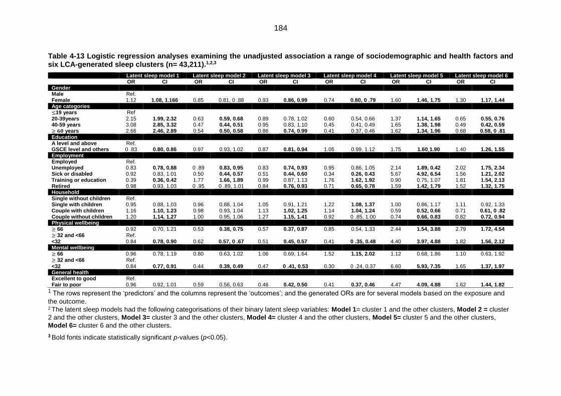
184
Table 4-13 Logistic regression analyses examining the unadjusted association a range of sociodemographic and health factors and six LCA-generated sleep clusters (n= 43,211).1,2,3
Latent sleep model 1 Latent sleep model 2 Latent sleep model 3 Latent sleep model 4 Latent sleep model 5 Latent sleep model 6 OR CI OR CI OR CI OR CI OR CI OR CI Gender Male Ref. Female 1.12 1.08, 1.166 0.85 0.81, 0 .88 0.93 0.86, 0.99 0.74 0.80, 0 .79 1.60 1.46, 1.75 1.30 1.17, 1.44 Age categories ≤19 years Ref
20-39years 2.15 1.99, 2.32 0.63 0.59, 0.68 0.89 0.78, 1.02 0.60 0.54, 0.66 1.37 1.14, 1.65 0.65 0.55, 0.76 40-59 years 3.08 2.85, 3.32 0.47 0.44, 0.51 0.95 0.83, 1.10 0.45 0.41, 0.49 1.65 1.38, 1.98 0.49 0.42, 0.59 ≥ 𝟔𝟎 years 2.66 2.46, 2.89 0.54 0.50, 0.58 0.86 0.74, 0.99 0.41 0.37, 0.46 1.62 1.34, 1.96 0.68 0.58, 0 .81 Education A level and above Ref. GSCE level and others 0 .83 0.80, 0.86 0.97 0.93, 1.02 0.87 0.81, 0.94 1.05 0.99, 1.12 1.75 1.60¸1.90 1.40 1.26, 1.55 Employment Employed Ref. Unemployed 0.83 0.78, 0.88 0 .89 0.83, 0.95 0.83 0.74, 0.93 0.95 0.86, 1.05 2.14 1.89, 0.42 2.02 1.75, 2.34 Sick or disabled 0.92 0.83, 1.01 0.50 0.44, 0.57 0.51 0.44, 0.60 0.34 0.26, 0.43 5.67 4.92, 6.54 1.56 1.21, 2.02 Training or education 0.39 0.36, 0.42 1.77 1.66, 1.89 0.99 0.87, 1.13 1.76 1.62, 1.92 0.90 0.75, 1.07 1.81 1.54, 2.13 Retired 0.98 0.93, 1.03 0 .95 0 .89, 1.01 0.84 0.76, 0.93 0.71 0.65, 0.78 1.59 1.42, 1.79 1.52 1.32, 1.75 Household Single without children Ref. Single with children 0.95 0.88, 1.03 0.96 0.88, 1.04 1.05 0.91, 1.21 1.22 1.08, 1.37 1.00 0.86, 1.17 1.11 0.92, 1.33 Couple with children 1.16 1.10, 1.23 0.98 0.93, 1.04 1.13 1.02, 1.25 1.14 1.04, 1.24 0.59 0.52, 0.66 0.71 0.61, 0 .82 Couple without children 1.20 1.14, 1.27 1.00 0.95, 1.06 1.27 1.15, 1.41 0.92 0 .85, 1.00 0.74 0.66, 0.83 0.82 0.72, 0.94 Physical wellbeing ≥ 66 0.92 0.70, 1.21 0.53 0.38, 0.75 0.57 0.37, 0.87 0.85 0.54, 1.33 2.44 1.54, 3.88 2.79 1.72, 4.54 ≥ 32 and <66 Ref. <32 0.84 0.78, 0.90 0.62 0.57, 0 .67 0.51 0.45, 0.57 0.41 0 .35, 0.48 4.40 3.97, 4.88 1.82 1.56, 2.12 Mental wellbeing ≥ 66 0.96 0.78, 1.19 0.80 0.63, 1.02 1.06 0.69, 1.64 1.52 1.15, 2.02 1.12 0.68, 1.86 1.10 0.63, 1.92 ≥ 32 and <66 Ref. <32 0.84 0.77, 0.91 0.44 0.39, 0.49 0.47 0 .41, 0.53 0.30 0 .24, 0.37 6.60 5.93, 7.35 1.65 1.37, 1.97 General health Excellent to good Ref. Fair to poor 0.96 0.92, 1.01 0.59 0.56, 0.63 0.46 0.42, 0.50 0.41 0.37, 0.46 4.47 4.09, 4.88 1.62 1.44, 1.82
1 The rows represent the ‘predictors’ and the columns represent the ‘outcomes’; and the generated ORs are for several models based on the exposure and
the outcome. 2 The latent sleep models had the following categorisations of their binary latent sleep variables: Model 1= cluster 1 and the other clusters, Model 2 = cluster
2 and the other clusters, Model 3= cluster 3 and the other clusters, Model 4= cluster 4 and the other clusters, Model 5= cluster 5 and the other clusters,
Model 6= cluster 6 and the other clusters.
3 Bold fonts indicate statistically significant p-values (p<0.05).

185
Table 4-14 Logistic regression analyses examining the confounder-adjusted association a range of sociodemographic and health factors and six LCA-generated sleep clusters (n= 43,211).1,2,3
Latent sleep model 1 Latent sleep model 2 Latent sleep model 3 Latent sleep model 4 Latent sleep model 5 Latent sleep model 6 OR CI OR CI OR CI OR CI OR CI OR CI Gender Male Ref. Female 1.12 1.08, 1.17 0.85 0.82, 0.88 0.93 0.86, 0.99 0.74 0.69, 0.78 1.61 1.47, 1.76 1.31 1.18, 1.46 Age categories ≤19 years Ref.
20-39years 2.14 1.98, 2.31 0.64 0.59, 0.68 0.89 0.78, 1.03 0.60 0.55, 0.66 1.35 1.13, 1.62 0.64 0.55, 0.76 40-59 years 3.07 2.84, 3.32 0.47 0.44, 0.51 0.95 0.83, 1.10 0.45 0.41, 0.50 1.64 1.36, 1.96 0.49 0.41, 0.58 ≥ 𝟔𝟎 years 2.67 2.46, 2.90 0.54 0.50, 0.58 0.85 0.74, 0.99 0.41 0.37, 0.46 1.63 1.35, 1.97 0.69 0.58, 0.82 Education A level and above Ref. GSCE level and others 0.81 0.78, 0 .84 0.98 0.94, 1.02 0.87 0.81, 0.94 1.09 1.03, 1.17 1.75 1.60, 1.91 1.36 1.22, 1.52 Employment Employed Ref. Unemployed 0.89 0.84, 0.95 0.89 0.83, 0.95 0.89 0.79, 1.00 0.91 0.82, 1.01 1.86 1.64, 2.11 1.77 1.52, 2.07 Sick or disabled 0.94 0.85, 1.04 0.52 0.46, 0.60 0.54 0.46, 0.63 0.34 0.27, 0.44 4.76 4.11, 5.51 1.45 1.45, 1.12 Training or education 0.63 0.57, 0.69 1.35 1.23, 1.48 1.01 0.84, 1.20 1.26 1.11, 1.42 1.03 0.82, 1.30 1.22 0.98, 1.52 Retired 0 .93 0.85, 1.01 0.98 0.89, 1.08 0.84 0.70, 0.99 0.76 0.65, 0.89 1.59 1.30, 1.94 1.53 1.19, 1.97 Household Single without children Ref. Single with children 1.26 1.16, 1.37 0.81 0.74, 0.88 1.01 0.86, 1.17 0 .99 0.87, 1.12 0.90 0.76, 1.06 0.80 0.65, 0.98 Couple with children 1.31 1.24, 1.39 0.89 0.83, 0.94 1.05 0.94, 1.17 0.96, 0.88, 1.05 0.63 0.56, 0.72 0.66 0 .56, 0.77 Couple without children 1.13 1.07, 1.19 1.03 0.97, 1.09 1.24 1.12, 1.38 0.94 0.86, 1.03 0.81 0.73, 0.91 0.88 0.77, 1.01 Physical wellbeing ≥ 66 1.04 0.79, 1.38 0.51 0.36, 0.72 0.59 0.38, 0.91 0.79 0.50, 1.24 2.13 1.33, 3.39 2.41 1.48, 3.94 ≥ 32 and <66 Ref. <32 0 .74 0.68, 0.79 0.75 0.68, 0.82 0.55 0.49, 0.63 0.57 0.48, 0.67 3.11 2.74, 3.53 1.75 1.47, 2.09 Mental wellbeing ≥ 66 0.94 0.76, 1.16 0.86 0.68, 1.10 1.16 0.75, 1.80 1.83 1.37, 2.43 0.86 0.52, 1.43 0.99 0.56, 1.73 ≥ 32 and <66 Ref. <32 0 .86 0.79, 0.93 0.48 0.43, 0.54 0.52 0 .46, 0.59 0.33 0.33, 0.41 4.75 4.24, 5.33 1.40 1.16, 1.70 General health Excellent to good Ref. Fair to poor 0.91 0.86, 0.96 0.66 0.61, 0.70 0.50 0.43, 0.51 0.48 0.43, 0.53 3.57 3.24, 3.94 1.54 1.35, 1.75
1 The rows represent the ‘predictors’ and the columns represent the ‘outcomes’; and the generated ORs are for several models based on the exposure and
the outcome. 2 The latent sleep models had the following categorisations of their binary latent sleep variables: Model 1= cluster 1 and the other clusters, Model 2 = cluster
2 and the other clusters, Model 3= cluster 3 and the other clusters, Model 4= cluster 4 and the other clusters, Model 5= cluster 5 and the other clusters,
Model 6= cluster 6 and the other clusters.
3 Bold fonts indicate statistically significant p-values (p<0.05).

186
4.5 Discussion
4.5.1 Limitations
In the temporal stability study, the differences in patterns observed between Waves
1 and 4 were evident for only two of the component sleep characteristics: sleep
duration and latency. These differences might simply reflect inherent variability in
either/both of these two sleep characteristics, or higher levels of respondent
error/reporting bias for these (as compared to the other separate) sleep
characteristics (Collins and Lanza, 2013, Lazarsfeld and Henry 1968). Certainly,
external environmental and contextual factors such as household structure (Fowler
et al, 2014), shift work (Åkerstedt, 2003) and/or day of the week/season of the year
(Anderson et al, 1994) are likely to affect both sleep duration and sleep latency,
and given these are both highly sensitive to changes in individual socio-
demographic circumstances (Arber et al, 2009), which themselves are prone to
vary over time and between Wave 1 and 4, such changes may indeed be
responsible for the three sleep pattern clusters with less than exactly the same
characteristics/composition in both Waves 1 and 4 of the UKHLS.
There is also the possibility that recall bias and/or classification error (i.e. the error
involved when categorising the continuous variable ‘sleep duration’) might have
undermined the accuracy of both of these sleep characteristics – not least because
estimating an ‘average’ sleep duration and sleep latency for the month preceding
questionnaire completion may prove rather more difficult than reporting the
frequency of disturbances or medication use etc (Van Den Berg et al, 2008,
Lockley et al, 1999). While this may well be true for sleep duration, the format of
the sleep latency question was actually very similar to that for the other ‘sleep
event’ questions (e.g. disturbances, coughing/snoring, and medication use). It is
therefore unlikely that recall bias or classification differentially affected sleep
latency alone. Instead, it may simply be that responses provided by UKHLS
participants who provided sleep data in both Waves 1 and 4 may have been
influenced by their prior exposure (in Wave 1) to sleep questionnaire items (i.e.
items with which they were initially unfamiliar; Backhaus et al, 2002, Buysse et al,
1989). However, the last of these possibilities also appears (un)likely given the lack
of an exact match between the six clusters identified in the analysis of Wave 1 data
(for the ‘temporal stability study) and the analysis of Wave 1 and 4 data (for the
‘correlates of sleep classes study), given that in both these instances the data
involved were provided only by respondents answering these sleep questions for
the very first time.

187
The LCA analyses used in the present chapter generated a total of six latent sleep
models using sleep data from n=45,141 participants in Wave 1 and /or Wave 4 who
would have been broadly representative of the UK population. However, adding
additional participants over and beyond those included in the temporal stability
study population (i.e. adding those who participated in Wave 1 or Wave 4 but not
both) resulted in the identification of new sleep patterns that had not been identified
earlier in the temporal stability study participants. These new patterns were
labelled: “short bad sleeper” (43.1%), “struggle-to-sleep-er” (6.2%) and “snoring
good sleeper” (1.7%). These additions might suggest the underlying presence of
(even) more sleep patterns amongst other populations, not least those younger
than 16 years (the youngest age of UKHLS participants) or those living in different
locations/contexts.
Nonetheless, the substantial temporal stability of sleep clusters over time was
clearly evident in the temporal stability study in the movement of participants
between classes/clusters rather than in any radical changes in the
composition/derivation of the classes themselves. This inter-class/cluster mobility
may, of course, reflect participants’ changing socio-demographic features or
environmental living conditions. Importantly, such changes of sleep patterns,
resulting primarily as a result of changes in an individual participant’s
characteristics over time, might lead one to conclude that the stability of sleep
might similarly differ amongst other populations were these to be subjected to
changes in their sociodemographic and health circumstances (such as that
occurring during pregnancy, where gestational age plays an important role in
predicting sleep).
In addition, it is clear from analyses conducted in the correlates of sleep classes
study that it is also likely that more (as yet ‘undiscovered’) sleep patterns are likely
to exist amongst those participants with missing data and/or those coming from
different populations/contexts (again, such as those who are younger or those
living in different latitudes/time zones and in contexts with very different
environmental and sociocultural characteristics).
4.5.2 Key findings
The analyses conducted in the present chapter examined both the presence and
temporal stability latent sleep patterns using data from Waves 1 and 4 of the
UKHLS. Latent class analysis of sleep data provided by exactly the same
respondents in both Waves 1 and 4 of the UKHLS demonstrated substantial
stability of sleep pattern classes/clusters over time – both in respect of the number
of classes (or ‘types’ of sleep patterns) and the specific characteristics of each of

188
these classes (i.e. the key features that distinguished one class from another).
However, sleep duration and sleep latency appeared to display slightly higher rates
of measurement/classification error than the five other sleep characteristics. The
importance of both for health (as evident in the literature) suggests that they need
to be measured with great (and perhaps more) care to address and ameliorate the
possibility of measurement error.
Meanwhile, it is worth pointing out that the vast majority of UKHLS participants
were members of cluster one – a class characterised by short sleep duration, poor
quality sleep and unfavourable sleep events. In contrast, the cluster that appeared
to characterise the least unfavourable sleep pattern (cluster three – which
characterised by long sleep duration, good quality sleep and absence of
unfavourable events) was only the third most common sleep pattern amongst
UKHLS participants. The low prevalence of a ‘favourable’ sleep pattern is not only
an interesting finding (given current interest in sleep and its relationship with
health).
This variability in the associations between sleep patterns and health suggests that
these clusters/classes might have substantial utility in determining any relationship
between sleep in pregnancy and pregnancy outcomes. This is because pregnancy
represents a stressful physiological condition that causes many women to describe
their perceived health as poor even in the absence of clinical disease or infirmity.
Meanwhile, the somewhat different directions of associations between individual
sleep characteristics, LCA-derived sleep patterns and sociodemographic/health
features might best be explained by the nature of sleep patterns themselves. Thus,
while individual sleep characteristics measure only one aspect of sleep, LCA-
derived sleep patterns are likely to offer more ‘holistic’ and comprehensive
assessments of sleep across more than simply one individual sleep characteristic.
The ‘long good sleeper’ category was considered the referent for the latent sleep
variable that will (also) be used in the analyses contained in the next two chapters.
This choice was made due to the similarity between ‘long good sleeper’ patterns
and individual sleep characteristic with respect to their relationship with health
indicators; as well as the fact that participants with a lower probability of displaying
‘long good sleeper’ sleep patterns were those individuals with a higher risk of
displaying sleep problems.
Compared to men, women were more likely to display ‘struggle to sleep-er’,
‘snoring good sleeper’ and ‘short bad sleeper’ sleep patterns. However, this
relation between sleep patterns and female gender might be under the influence
of other sociodemographic and health features not examined in the present chapter

189
(including pregnancy, which will be studied in the next two chapters). Unfortunately,
then, it remains unclear why women (particularly those who were not pregnant, as
will become clear later) were prone to these less ‘favourable’ sleep patterns and
further investigations are warranted to better understand this.
Knowing that the latent sleep variable generated using LCA of UKHLS sleep
module data was significantly associated with sociodemographic and health
features confirmed the usefulness of the hypothesised DAG (originally postulated
in Chapter 2; Section 2.4, page 59). Likewise, the association between sleep and
sociodemographic/health confirmed the possibility that the latter might act as
potential confounders in the relation between sleep and pregnancy outcomes (not
least because many of these sociodemographic/health variables are also known
to be risk factors for poorer pregnancy outcomes). However, the second half of the
DAG (i.e. to the right hand side of ‘sleep’) which summarised the hypothesised
association between sleep and pregnancy outcomes still requires closer
examination – an issue that will be examined in the next chapters.
Although the findings presented in the present chapter are ‘powerful’ (based as
they are on a large sample size and the number of individual sleep characteristics
available for analysis), these findings remain constrained by the subjective
measurement of sleep, the (somewhat uncertain) choice of referent sleep
categories, and the presence of substantial missing data. Therefore, better data
with better measurement, and better specification of referent sleep categories
might further improve the value of these analyses, and may (for example) identify
other sleep patterns that were not evident with the data available for the present
chapter’s analyses. As such it is important to stress that these results might not be
generalizable to other populations (with contrasting sociodemographic and health
features) or to studies using alternative sources of sleep data. Nonetheless, by
including as many participants as possible the analyses presented in this chapter
ensured that these were able to discover a substantial number and variety of sleep
patterns; and these patterns suggest a similar approach may have utility for further
studies examining sleep amongst UKHLS participants (or other, similar datasets)
4.5.3 Conclusion
Latent class analysis generated 6 clusters with distinct patterns and different sizes
as the membership of some sleep clusters was more common than others. The
latent sleep clusters were quite stable over time except, to a modest extent, with
respect to the relative contributions made by sleep duration and sleep latency in
some of the clusters – variation that might suggest a role for more objective
measures of these variables in future studies of this nature. However, over time,

190
some participants’ sleep patterns changed (and that such changes were more
common from/to some sleep patterns than others – suggesting that some might be
more ‘transitory states’ and others more ‘stable’, perhaps due to their varying
sensitivity to changes in the sociodemographic and health circumstances
prevailing at different time points. Both these clusters and each the individual sleep
characteristic display important associations with sociodemographic and health
variables, even after adjustment for potential confounding, although these
associations are different for sleep clusters and individual sleep characteristics,
suggesting that clusters and characteristics capture distinct aspects of sleep, and
supporting the possibility that latent sleep clusters represent more holistic
assessments of overall ‘sleep patterns’. However, this suggestion would not
change the hypothesized DAG (in which ‘sleep’ is represented by a single
variable), since the association between latent sleep, sociodemographic
characteristics and health still exist. In the chapters that follow, the distribution of
sleep clusters identified in the present chapter are examined in populations of
pregnant women, and are then compared to sleep characteristics as potential
correlates of/precursors to a range of pregnancy outcomes.
4.5.4 Recommendation
Further research is required in this area to describe sleep patterns using LCA
because, at the time of this study (and as far as is evident from the literature
examined during the course of the present thesis), no research has previously
described sleep using LCA to describe ‘sleep patterns’ in this way before. However,
the analyses presented in the present chapter do suggest that adopting a ‘latent
sleep approach’ may be more useful in defining sleep than the classic approach
(using separate, individual sleep characteristics, or composite scores such as the
PSQI ‘sleep quality index’); and that the latent sleep categories generated can (and
did) have very different patterns of association with sociodemographic and health-
related characteristics when compared to analyses using separate, individual sleep
characteristics .
Additional sleep research using LCA would also facilitate the comparison of sleep
patterns observed between different populations, as well as furthering
understanding as to which covariates might influence which of these sleep
patterns. Meanwhile, the measurement of sleep clearly requires careful
consideration, particularly when choosing the measurement tool used, and
especially regarding sleep duration and latency (both of which displayed some
variation in their contributions to sleep patterns over time). Moreover, thoughtful
consideration should be given when choosing the referent categories for both

191
individual sleep variables and LCA-derived sleep clusters, since the results showed
that the choice of the referent category can affect the pattern of association(s)
observed between sleep, sociodemographic characteristics and health-related
features. Finally, as ever, better quality data is required for such studies,
particularly regarding the missingness of data. These considerations, together with
wider acceptance amongst researchers regarding the quality of their data, the
power of their sample sizes, and the number of hypotheses examined, might be
required to temper the number of clusters derived, and the certainty with which the
best-fitting number of clusters are selected for subsequent analytical use.

192
Chapter 5 The relationship between sleep and birth
outcomes in the UK pregnant women: UKHLS
5.1 Introduction
A few UK-based sleep studies have reported higher rates of sleep ‘problems’ in
women than men (Arber et al., 2009, Hislop and Arber, 2003), attributing these to
possible hormonal and/or psychosocial causes. However, amongst pregnant
women, sleep is widely considered to become more problematic due to changing
hormone levels, and anatomical consequences of an enlarged uterus (Hedman et
al., 2002, Hertz et al., 1992). Some authors have also suggested that the increase
in sleep problems during pregnancy are often associated with poorer pregnancy
outcomes. Nonetheless, little is known about the pathophysiology of how sleep
problems might affect the mother and her foetus or might correlate with poor
pregnancy outcomes (albeit with the exception of SBD, which is known to affect
cardiovascular and respiratory functions). If a broader relationship between the
sleep and poor pregnancy outcomes were to be established, this might identify
potential interventions for preventing or attenuating some potentially serious
pregnancy complications simply by improving (or otherwise modifying) maternal
sleep.
As discussed in the preceding chapter which reviewed previous studies of this
topic, despite the broad consensus these suggest of a link between less favourable
sleep and poor pregnancy outcomes – few of these studies examined the full
breadth of sleep-related measures available (i.e. few had measured more than a
few sleep characteristics). Moreover, none had attempted to examine sleep more
‘holistically’ using a combination of sleep characteristics to identify latent ‘sleep
patterns’ (as the present thesis has done). Furthermore, the present thesis could
find no information in the literature regarding pregnant women in the UK and any
possible association between sleep and pregnancy outcome – most of the
published studies having been conducted in the US.
The aim of this study was therefore to examine both a wide range of sleep
characteristics (i.e. the 7 discrete sleep characteristics generated within the
UKHLS sleep module) and the LCA sleep patterns identified in the preceding
chapter, in a population-based sample of pregnant women from the UK population,
and thereafter to examine their relationship with poor pregnancy outcomes.
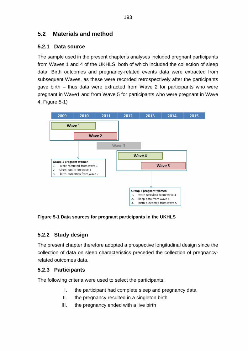
193
5.2 Materials and method
5.2.1 Data source
The sample used in the present chapter’s analyses included pregnant participants
from Waves 1 and 4 of the UKHLS, both of which included the collection of sleep
data. Birth outcomes and pregnancy-related events data were extracted from
subsequent Waves, as these were recorded retrospectively after the participants
gave birth – thus data were extracted from Wave 2 for participants who were
pregnant in Wave1 and from Wave 5 for participants who were pregnant in Wave
4; Figure 5-1)
Figure 5-1 Data sources for pregnant participants in the UKHLS
5.2.2 Study design
The present chapter therefore adopted a prospective longitudinal design since the
collection of data on sleep characteristics preceded the collection of pregnancy-
related outcomes data.
5.2.3 Participants
The following criteria were used to select the participants:
I. the participant had complete sleep and pregnancy data
II. the pregnancy resulted in a singleton birth
III. the pregnancy ended with a live birth

194
Women with multiple pregnancy were excluded because their number was small
(n=3) hence it was not possible to adjust for them in the analytical models (it being
likely that multiple pregnancy would affect both the risk of poor sleep and poor
pregnancy outcomes). Additionally, the sample was restricted to women whose
pregnancies ended in a live birth simply because there were no pregnancy- related
data for any pregnant women who subsequently suffered a termination or still birth.
Pregnant participants were identified in both Waves (i.e. 1 & 4) using each of the
steps shown in the following sub-section, though only those for whom sleep data
were available were included in the analyses that follow.
5.2.3.1 Identifying pregnant participants in Wave 1
The pregnant women in Wave 1 were identified according to their responses to the
following questions:
I. The first question used was in Wave1, and stated: “Do you think you will
have [any more/any] children?” The selected participants responded as
follows: “Self/partner currently pregnant” [included only females].
II. The second question was in Wave 2, and stated: “Since [ff_Int_Date] have
you been pregnant at all, even if this did not result in a live birth?” The
selected participants responded as follows: “Pregnant at last interview”.
5.2.3.2 Identifying pregnant participants in Wave 4
The participants in Wave 4 were also identified based on their responses to two
questions:
I. The first question was from the Wave 4 questionnaire, and stated: “Last
time we interviewed you, you were pregnant. Did this/your next
pregnancy result in a live birth with a normal delivery or by caesarean
section?” Currently pregnant women selected the response “current
pregnancy”.
II. The second question was from the Wave 5 questionnaire, and stated: “The
next questions are about any children you may have had. Since
[ff_Int_Date], have you been pregnant at all, even if this did not result
in a live birth?” Women who had been pregnant in the preceding Wave
(Wave 4) selected the response “pregnant at last interview”.
5.2.4 Measurements
5.2.4.1 Sleep characteristics
Sleep data were gathered using the self-completed UKHLS Sleep Module. In the
analysis presented in the present chapter, sleep duration was categorised into the

195
following: long sleep (>9 hours), short sleep (<6 hours) and reference range (≥6
and ≤9 hours) to ensure that these analyses were capable of assessing the
possibility of a U-shaped relationship between sleep duration and (poor) pregnancy
outcomes. For items relevant to different sleep ‘events’ (i.e. latency, disturbance,
snoring or coughing, daytime sleepiness, use of sleep-related medication), these
were each categorised as binary variables based on the absence or presence of
the events in question. Finally, sleep quality was simply categorised as good vs.
bad.
Reducing each of these polytomous variables to binary categorical variables was
needed to ensure that the analyses could accommodate the limited number of
pregnant UKHLS participants in some instances. For similar reasons, an ‘absence
vs. presence’ cut off point was chosen rather than an ‘habitual’ versus ‘non-
habitual’ cut off to ensure there were sufficient numbers of participants in both
categories and to minimise the possible effect of measurement error in the
reporting of the frequency of the events.
5.2.4.2 Sleep clusters
Sleep clusters were assigned to participants from the UKHLS using the algorithm
generated from the latent class analysis study which was discussed in detail
previously in Chapter 4. The algorithm used (Appendix, Section 8.3.5, page 319)
was generated in table format using Latent Gold Software (Statistical Innovations
Inc., 2009) and the table was then transformed into commands within STATA
(StataCorp., 2013). The STATA commands were then applied to the responses of
study participants to the seven sleep questions (the answers to each of which had
been recoded so as to be the same as that categorised for the analyses in which
the sleep clusters were generated in Chapter 4). As described earlier in the thesis,
these six sleep clusters were labelled: short bad sleeper, long moderate sleeper,
long good sleeper, disturbed bad sleeper, struggle-to-sleep-er, and snoring good
sleeper.
5.2.4.3 Birth outcomes
In the UKHLS, the birth outcomes on which data were available were: birth weight,
mode of delivery and preterm delivery. The birth outcomes of women who were
pregnant in Wave 1 were obtained from responses presented in Wave 2, and the
outcomes of pregnant women in Wave 4 were obtained from responses presented
in Wave 5 (see Figure 5-1). Each of these outcome variables were re-categorised
into binary categorical variables so that these were amenable for analytical
techniques that generated the OR associated with the risk of developing poor
pregnancy outcomes.

196
For birth weight this first involved some standardisation of units, since this was
recorded in two different units (i.e. grams, ounces and pounds), all of which were
standardised into grams. For the analyses that follow, birth weight was then
categorised as low birth weight (<2500 grams), macrosomia (>4000 gram) or
normal weight (≥2500 and ≤4000 grams). The cut-off points were chosen based
on the WHO criteria for ‘abnormal’ birth weight (United Nations Children’s Fund
and World Health Organization, 2004).
Caesarean delivery was categorized as caesarean delivery (which included both
elective and emergency delivery) vs. vaginal delivery (which included both
assessed and non-assessed vaginal delivery). This categorisation was chosen due
to the absence of any further information regarding the reasons for caesarean
delivery or any other difficulties encountered with the natural birth.
Preterm delivery was defined as any delivery prior to 37 weeks of gestation, again
based on the WHO definition (World Health Organization, 2015). Preterm delivery
was thereby categorised into preterm delivery and term delivery (which included
both date and post-date deliveries).
For further details about the extraction of variables from the UKHLS data set and
the coding of these, please refer to the Appendix (Chapter 8, Section 8.4, page
343).
5.2.4.4 Covariates
Confounders were identified from amongst those covariates that were available
within the UKHLS data set. In the first instance, a simple Directed Acyclic Graph
(DAG) was drawn to generate a visual guide for selecting those covariates acting
as confounders from amongst the large number of covariates available (Figure
5-2). The covariates selected included sociodemographic features, pre-pregnant
maternal health conditions and parity – all of which were judged to have preceded
the exposures examined in the present chapter’s analysis (i.e. sleep during
pregnancy).
In regard to the potential role of behavioural risk factors for poor pregnancy
outcomes (i.e. smoking and alcohol), some of which may have become established
prior to the measurement of the exposure, the decision was taken not to adjust for
these in the multivariable analyses that follow primarily because they were
collected retrospectively (i.e. after birth), and it was therefore not known if their
measurement preceded or followed the measurement of sleep.

197
Figure 5-2 Simplified DAG illustrating shows the temporal relationship between the covariates available in the UKHLS dataset.
Sociodemographic features and the data on maternal health condition were
extracted from the same UKHLS wave as that providing the sleep data (that is, in
Waves 1 and 4, respectively).
As before, the number of categories for each of the covariates included in these
analyses was reduced into two (i.e. each were re-categorised as binary variables)
to facilitate the inclusion of as many confounders as possible (given the modest
sample sizes available). In each instance, the cut-off points chosen were based on
the distribution of the data, although a secondary (yet equally important
consideration) was to also try to reduce the loss of meaning and the risk of (further)
categorisation error. Indeed, for this reason, maternal (participant) age was
retained for use as a continuous variable.
Elsewhere, ethnicity was categorised based on its classification within the NICE-
generated GDM risk scoring, in which women classified as having a ‘White’
ethnicity is considered to be at ‘low risk’ (of GDM) whilst those classified as having
other (black and minority ethnic group ethnicities - such as South Asian and Black)
are considered to be at higher risk.
Employment status was included in the analyses after re-categorisation into
‘currently working’ vs. ‘currently not working’. Likewise, education was categorised
into ‘lower’ vs. ‘higher’ educational attainment. Cohabitation was also categorised
into a binary variable as being either ‘had’ or ‘did not have’ a partner. Meanwhile,
pregnant women who reported having any of the following health conditions were
coded as having poor(er) pre-pregnant health: asthma, arthritis, congestive heart
failure, coronary heart disease, angina, heart attack or myocardial infarction,
stroke, emphysema, hypothyroidism or under-active thyroid, chronic bronchitis,

198
any liver condition, cancer or malignancy, diabetes mellitus (but not GDM),
epilepsy, high blood pressure, clinical depression, hyperthyroidism or an over-
active thyroid. Finally, parity was simply categorised into nulliparous vs.
multiparous.
For further details about the extraction and (re)coding of covariates from the
UKHLS data sets, please refer to the Appendix (Chapter 8, Section 8.4.3, page
344).
5.2.5 Ethical considerations
Ethical approval for the main survey of the UKHLS was obtained from the Ethics
Committee of the University of Essex on 6 July 2007 for Wave 1 and on 17
December 2010 for Wave 4 (Gundi, 2016).
Access to the ‘special license version’ of the UKHLS dataset was obtained in March
2015 by the candidate and their supervisors. However, data released under the
special license version were not used due to the very poor quality of data for each
of the variables of interest examined (in particular, those variables that might have
helped to generate estimates of the gestational age at which participants in Wave
1 responded to the items on sleep [and other covariate characteristics]).
5.3 Analyses
5.3.1 Descriptive analysis
5.3.1.1 Missing data
The distributions of missing data, as compared to the distribution of complete data,
were tabulated to facilitate closer inspection. Missing data were examined for the
possibility that these were missing at randomand were then treated by listwise
deletion.
5.3.1.2 Participant’s characteristics
Frequency and percentage tables were used to display the distribution of each of
the characteristics examined for participants included in the present chapter’s
analyses.
5.3.2 Regression analysis
Adjusted and unadjusted logistic regression models were used to assess the
relationship between sleep and pregnancy outcomes. As mentioned in Section
5.2.4.2, the latent sleep variable that was included in the present chapter’s analysis
comprised the six categories of the latent sleep variable that had ‘long good

199
sleeper’ as the referent, and in which participants were allocated membership to
one of the six sleep clusters by applying the LCA-generated algorithm (as
discussed in Chapter 4) using participants’ responses to the seven sleep questions
presented in the UKHLS sleep module.
The estimation method used in the logistic regression analysis was the penalized
maximum likelihood estimation (Firth, 1993; see Chapter 2, Section 2.5.1.1, page
72). STATA.13 software was used for all of these analyses (StataCorp., 2013).
A dedicated DAG was used to assist in identifying the minimal sufficient set of
covariates necessary to adjustment for any confounding associated therewith. This
DAG was drawn using the open-source software DAGitty (see Textor et al., 2017).
5.4 Results
5.4.1 Included participants
The number of pregnant UKHLS participants identified from Wave 1 was 532 and
from Wave 4 was 408 (Figure 5-3 and Figure 5-4). However, the final number of
participants included in the study was only 294 since many had missing data on
the selected exposures, outcomes and/or covariates. This final number was
achieved by merging data from each wave and thereafter excluding data from any
duplicate participants occurring (not only in Wave 1 but also) in Wave 4 (- meaning
that these participants’ first responses to the sleep questionnaire, from Wave 1,
remained in the analyses that follow, see: Figure 5-5).

200
Figure 5-3 Flowchart showing how pregnant women were included or excluded from data generated during Waves 1 and 2 of the UKHLS

201
Figure 5-4 Flowchart showing how data from pregnant women were included and excluded from the datasets generated during Waves 4 and 5 of the UKHLS

202
Figure 5-5 Flowchart showing pregnant women included or excluded after samples and data from Waves 1 and 4 of the UKHLS were merged
5.4.2 Descriptive analysis results
5.4.2.1 Missing data
There was no visible association between missingness amongst the sleep and
pregnancy outcomes variables, and the distribution of sleep characteristics in the
women with missing data on birth outcomes was similar to the distribution of sleep
characteristics amongst women with complete data on birth outcomes (Appendix,
Section 8.4.4, page 346, Table 8-22). Similarly, women with missing sleep data had
birth outcome distributions that appeared broadly similar to those of women with
complete sleep data (Appendix, Section 8.4.4, page 346, Table 8-23). In addition,
there did not appear to be any clustering of missing data amongst particular groups of
participants, since women with missing data on sleep or health had a very similar
distribution of sociodemographic characteristics to those women with complete data
on sleep and health (Appendix, Section 8.4.4, page 346, Table 8-24).
Merging w1 and w4 pregnant
populations with live birth singleton
pregnancies = 940
• wave 1 =532
• wave 4 =408
Participants with complete outcomes
data =545
Live birth singleton pregnancies in
wave 1 and 4 =921
Duplicates from wave 4 =19
Missing outcomes data (i.e. birth
weight, preterm delivery , cesarean
delivery) =376
Participants with complete covariates
data= 338
Missing covariates data (i.e. age,
parity, alcohol, smoking, employment,
education, cohabiting, health
condition) =207
Pregnant women with complete
medical and sleep data = 294
Missing sleep data =44
Included participants (n=294) Excluded participants

203
5.4.2.2 Sleep characteristics
As evident in Table 5-1, the distribution of sleep characteristics amongst women with
complete data on each of the sleep and health variables followed a distribution that
was similar to the sleep characteristics of all eligible pregnant women. Overall, the
pregnant women were more likely to display sleep durations falling between 6 and 9
hours a day. In addition, they reported low rates of the following events: snoring,
daytime sleepiness and (particularly) use of sleep-related medication. In contrast, they
reported higher rates of sleep latency and disturbance.
As regards the latent sleep clusters, the commonest sleep pattern was ‘short bad
sleeper’ whilst the least common was ‘disturbed bad sleeper’. Only 12.9% (n=38) of
the pregnant UKHLS participants reported an absence of unfavourable sleep events
and had sleep patterns characterised as long good (Table 5-1).
Table 5-1 Distribution of sleep characteristics amongst pregnant UKHLS participants
Singleton livebirth pregnant women with
complete data
All singleton livebirth pregnant population
n=294 % n=921 %
Sleep duration
Short sleep (<6) 37 12.59 106 11.51 Reference range (6-9)
229 77.89 659 71.55
Long sleep (>9) 28 9.52 55 5.97 Missing 0 0 101 10.97 Latency Absent 113 38.44 313 33.98 Present 181 61.56 509 55.27 Missing 0 0 99 10.75 Disturbance Absent 41 13.95 128 13.9 Present 253 86.05 698 75.79 Missing 0 0 95 10.31 Snoring or coughing
Absent 226 76.87 626 67.97 Present 68 23.13 181 19.65 Missing 0 0 114 12.38
Day sleepiness
Absent 247 84.01 692 75.14 Present 47 15.99 125 13.57
Missing 0 0 104 11.29 Medication Absent 282 95.92 786 85.34 Present 12 4.08 50 5.43 Missing 0 0 85 9.23 Quality Good 217 73.81 589 63.95
Bad 77 26.19 249 27.04
Missing 0 0 83 9.01 Sleep clusters
Short bad sleeper 162 55.1 393 42.67 Long moderate sleeper
27 9.18 87 9.45
Long good sleeper 38 12.93 95 10.31 Disturbed bad sleeper 11 3.74 32 3.47 Struggle to sleep-er 36 12.24 106 11.51 Snoring good sleeper 20 6.8 66 7.17 Missing 0 0 142 15.42

204
5.4.2.3 Birth outcomes
The mean birth weight of pregnant women in the present analyses was 3,439 g
(SD=597, minimum=1,814, maximum=4,320). Only 19.4% (n=15) of the pregnant
women with macrosomic babies delivered via CS, while 88.2% (n=15) of low birth
weight babies were born premature. Nonetheless, the rate of term deliveries was
around 75% (n=221), one quarter of which were caesarean deliveries (n=55, 24.9%).
Unfortunately, only 113 women in the UKHLS study with complete data reported their
gestational age: 23 of these women participated while they were in their first trimester
of pregnancy, 43 were in their second trimester, and 47 women were in their third
trimester.
A summary of the distribution of birth outcomes amongst pregnant UKHLS participants
is presented in Table 5-2.
Table 5-2 Distribution of birth outcomes amongst pregnant UKHLS participants
Singleton livebirth pregnant with complete data
All singleton livebirth pregnant population
n=294 % n=921 %
Macrosomia ≤ 4000 gm 252 85.71 426 46.25
>4000 gm 42 14.29 119 12.92 Missing 0 0 376 40.83 Low birth weight
Birth weight ≥ 2500 gm 277 94.22 292 31.7
Birth weight <2500 gm 17 5.78 253 27.47
Missing 0 0 376 40.83 Preterm labour
Term 221 75.17 672 72.96 Preterm 73 24.83 121 13.14
Missing 0 0 128 13.9 Mode of delivery
Vaginal 217 73.81 594 64.5 Caesarean 77 26.19 192 20.85
Missing 0 0 135 14.66
5.4.2.4 Sociodemographic features and health
As summarised in Table 5-3, the majority of the participants examined were in their
twenties and thirties, were nulliparous and had a partner. From the 34 participants who
did not work around the time sleep was measured; 31 were on maternity leave and
three were on long-term sickness or disability leave.
Nearly 13% of the participants reported smoking during pregnancy, whereas around
25% of the non-smokers were ex-smokers (n= 61). Twelve participants smoked more
than 10 cigarettes a day during their first trimester, and 6 participants smoked more
than 10 cigarettes during their second and third trimesters. Approximately 75% of the
participants did not consume alcohol during their pregnancy, and around half of those
who consumed alcohol (n= 47) consumed two or less units of alcohol per week.
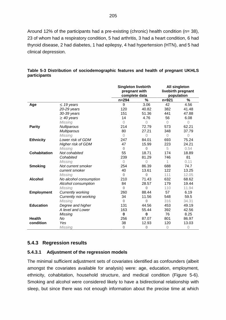
205
Around 12% of the participants had a pre-existing (chronic) health condition (n= 38),
23 of whom had a respiratory condition, 5 had arthritis, 3 had a heart condition, 6 had
thyroid disease, 2 had diabetes, 1 had epilepsy, 4 had hypertension (HTN), and 5 had
clinical depression.
Table 5-3 Distribution of sociodemographic features and health of pregnant UKHLS participants
Singleton livebirth pregnant with complete data
All singleton livebirth pregnant
population
n=294 % n=921 %
Age ≤ 19 years 9 3.06 42 4.56
20-29 years 120 40.82 382 41.48 30-39 years 151 51.36 441 47.88 ≥ 40 years 14 4.76 56 6.08 Missing 0 0 0 0
Parity Nulliparous 214 72.79 573 62.21 Multiparous 80 27.21 348 37.79 Missing 0 0 0 0
Ethnicity Lower risk of GDM 247 84.01 693 75.24 Higher risk of GDM 47 15.99 223 24.21 Missing 0 0 5 0.54
Cohabitation Not cohabited 55 18.71 174 18.89 Cohabited 239 81.29 746 81 Missing 0 0 1 0.11
Smoking Not current smoker 254 86.39 688 74.7 current smoker 40 13.61 122 13.25 Missing 0 0 111 12.05
Alcohol No alcohol consumption 210 71.43 632 68.62 Alcohol consumption 84 28.57 179 19.44 Missing 0 0 110 11.94
Employment Currently working 260 88.44 57 6.19 Currently not working 34 11.56 548 59.5 Missing 0 0 316 34.31 Education Degree and higher 131 44.56 453 49.19 A level and Lower 163 55.44 392 42.56 Missing 0 0 76 8.25 Health condition
No 256 87.07 801 86.97 Yes 38 12.93 120 13.03
Missing 0 0 0 0
5.4.3 Regression results
5.4.3.1 Adjustment of the regression models
The minimal sufficient adjustment sets of covariates identified as confounders (albeit
amongst the covariates available for analysis) were: age, education, employment,
ethnicity, cohabitation, household structure, and medical condition (Figure 5-6).
Smoking and alcohol were considered likely to have a bidirectional relationship with
sleep, but since there was not enough information about the precise time at which

206
these variables were measured (particularly in relation to the measurement of sleep),
both were considered potential mediators and were therefore not included in the
covariate adjustment sets used.
An additional covariate adjustment set was included that only had those variables
available in both the Scott/Ciantar study and UKHLS. Although this analysis was
considered under-adjusted (since it lacked confounders available in one, though not
both, of these datasets), it was nonetheless conducted to permit a direct comparison
of the regression analyses’ results between these two studies. The common
adjustment set included the following confounders: age, ethnicity, education,
cohabiting and health.
Unfortunately, it was not possible to include BMI in the covariate adjustment sets
because so few participants had data (only those who had participated in Wave1
where weight and height were recorded). Late pregnancy complications were also not
available in the UKHLS data set, though these were likely to have been mediators in
the relationship between sleep and pregnancy outcomes.
As for gestational age at questionnaire completion and BMI, it was not possible to
consider the inclusion of neonatal sex in the multivariable analyses since this
information was rarely available.
With regard to the various pregnancy outcomes used, it was clear that preterm delivery
was likely to have affected birth weight. However, because preterm delivery was also
considered a mediator for any relation between sleep and birth weight it was not
included in the analyses of these relationships.
Given there was little detail about previous obstetric history (e.g. previous macrosomia
or caesarean section), and no data on late pregnancy complications (e.g. pregnancy
induced hypertension) neither could be considered for inclusion in the multivariable
analyses undertaken in the present chapter.

207
Figure 5-6 Directed acyclic graph summarizing the minimal sufficient covariate adjustment set required to adjust for confounding in regression models examining the relationship between sleep and maternal outcomes.

208
5.4.3.2 The relation between sleep and birth outcomes
In general when examining each of the seven specific sleep characteristics, the odds
of macrosomia was higher amongst pregnant women with short sleep,
coughing/snoring and disturbed sleep (Table 5-6); whilst, the odds of LBW neonates
was higher amongst women who coughed/snored, used medication to assist with
sleep, and who experienced protracted sleep latency (Table 5-7). In contrast, the odds
of preterm delivery exhibited a relationship with unfavourable sleep amongst all of the
individual sleep characteristics, with the exception of daytime sleepiness (Table 5-5).
A heightened odds of caesarean section, however, was only associated with sleep
latency and coughing/snoring (Table 5-4). That said, it is important to note that the
estimated risk of pregnancy outcomes lacked precision, as reflected by a wide 95%
confidence interval, as a result of the underpowered analysis. At the same time, some
of the 95% CIs were wider than others due to the difference in the distribution of the
unfavourable sleep events and pregnancy outcomes amongst the study’s participants.
As regards the LCA-derived sleep patterns, the odds of preterm delivery was higher
amongst women classified as long good sleepers (Table 5-5), whilst the odds of
caesarean section was higher amongst women classified as short bad sleepers, long
moderate sleepers, disturbed bad sleepers, and struggle-to-sleep-ers (Table 5-4).
Meanwhile, the odds of macrosomia was higher in struggle to-sleep-ers and snoring
good sleepers (Table 5-6), in contrast to the elevated odds of low birth weight amongst
long good sleepers (Table 5-7).). Again, these estimated ORs lacked precision which
made it difficult to interpret the results with a preferred level of confidence and
certainty.
Nonetheless, it is possible to claim that coughing/snoring had the most (and strongest)
relation with an elevated odds of all poor pregnancy outcomes – while daytime
sleepiness was generally accompanied by a lower odds of poor pregnancy outcomes.
The odds of preterm delivery was lower amongst women with less favourable sleep
patterns, except for those who were short bad sleepers; whilst the risk of caesarean
delivery was higher across all sleep patterns with the exception of those labelled
snoring good sleepers.
In the following sections of this results section, the relation between sleep and
pregnancy outcomes will be presented using ORs as well as 95% CIs to reflect the
level of confidence and precision of the OR estimates. The associated p-values will
not be presented since multiple testing was involved, and might therefore increase the
chance of type I error (reflected by a significant p-value). However, there were
occasionally statistically ‘significant’ findings which have been highlighted using bold

209
text in the results tables that follow, though once again these should be interpreted
with caution since they might merely be due to chance.
5.4.3.2.1 Mode of delivery
Latency (OR=1.25, CI=0.72, 2.17) and snoring (OR=1.61, CI=0.89, 2.90) were
accompanied by an elevated risk of caesarean delivery. In contrast, long duration
(OR= 0.56, CI= 0.19, 1.60) and disturbance (OR=0.69, CI=0.33, 1.43) were
accompanied by a reduced risk of caesarean delivery. Short duration (OR=1.02, CI=
0.47, 2.47) and usage of medication (OR = 1.09, CI = 0.30, 3.89) showed a modest
relation with caesarean delivery (Table 5-4).
In regards to LCA-derived sleep patterns, the risk of caesarean delivery increased with
all sleep patterns except snoring good sleep pattern (OR=0.88, CI=0.24, 3.25) when
compared to participants who had long good sleep pattern (Table 5-4).
5.4.3.2.2 Preterm delivery
After adjustment of possible confounders, an elevated risk of preterm delivery was
accompanied by all unfavourable sleep characteristics except next day sleepiness
(OR=0.40, CI=0.17, 0.96; Table 5-5)
In regards to LCA-derived sleep patterns, short bad sleepers (OR=0.79, CI=0.36,
1.72), long moderate sleepers (OR=0.50, CI=0.15, 1.69) and disturbed bad sleepers
(OR=0.34, CI=0.05, 2.17) had a lower risk of preterm delivery compared to participants
who had absent unfavourable events (i.e. long good sleepers) whilst, struggle to sleep-
ers and snoring good sleepers had almost similar odds of preterm delivery compared
to long good sleepers.
5.4.3.2.3 Macrosomia
Latency was accompanied by a reduced risk of macrosomia (OR=0.76, CI=0.39, 1.48)
in contrast to snoring, which had a higher risk of macrosomia (OR= 2.12, CI=1.02,
4.41). The other sleep characteristics showed modest effect on the risk of
macrosomia; their ORs were almost 1.0 (Table 5-6)
Compared to long good sleepers, the risk of macrosomia in the UKHLS pregnant
participants was higher in the struggler to sleep-ers (OR=1.26, CI=0.36, 4.40) and
snoring good sleepers (OR=1.59, CI=0.39, 6.38); whereas, it was lower in the Long
moderate sleepers (OR=0.97, CI=0.23, 4.19) and disturbed bad sleepers (OR=0.28,
CI=0.14, 5.49).

210
5.4.3.2.4 Low birth weight
Short (OR=0.61, CI=0.11, 3.43) and long (OR=0.79, CI=0.13, 4.66) duration and
quality (OR=0.67, CI=0.20, 2.24) were accompanied by a small risk of low birth weight.
Snoring (OR=2.02, CI=0.73, 5.55) and medication (OR=3.70, CI=0.80, 17.25) were
accompanied by an elevated risk of low birth weight (Table 5-7).
In regards to sleep patterns, the risk of low birth weight was lower for all five sleep
patterns compared to long good sleep patterns (Table 5-7)

211
Table 5-4 Logistic regression model examining the relationship between caesarean delivery and each of the seven specific sleep characteristics and six sleep patterns. All results are presented as odds ratios (OR) with 95% confidence intervals (CI). 1,2
Cesarean Delivery Models Level of Adjustment Unadjusted model Adjusted model1 Adjusted model2
OR CI OR CI OR CI
Caesarean delivery model 1: caesarean delivery and short sleep duration
≥ 6 hours Referent
< 6 hours 0.91 0.50, 1.65 1.10 0.51, 2.40 1.02 0.47, 2.47
Caesarean delivery model 2: caesarean delivery and long sleep duration ≤ 9 hours Referent > 9 hours 0.48 0.17, 1.37 0.56 0.19, 1.65 0 .56 0 .19, 1.60 Caesarean delivery model 3: caesarean delivery and sleep duration Continuous 0.88 0.72, 1.07 0.93 0.76, 1.14 0.94 0.77, 1.16 Caesarean delivery model 4: caesarean delivery and sleep latency Absent Referent Present 1.21 0.71, 0.71 1.27 0.73, 2.20 1.25 0.72, 2.17 Caesarean delivery model 5: caesarean delivery and sleep disturbance Absent Referent Present 0.72 0.36, 1.46 0.66 0.32, 1.38 0.69 0.33, 1.43 Caesarean delivery model 6: caesarean delivery and snoring (and/or coughing) Absent Referent Present 1.64 0.91, 2.93 1.61 0.89, 2.93 1.61 0.89, 2.90 Caesarean delivery model 7: caesarean delivery and sleep medication Absent Referent Present 1.03 0.29, 3.61 1.02 0.29, 3.63 1.09 0.31, 3.89 Caesarean delivery model 8: caesarean delivery and next day sleepiness Absent Referent Present 0.55 0.25, 1.22 0.59 0.26, 1.31 0.57 0.26, 1.27 Caesarean delivery model 9: caesarean delivery and sleep quality Good Referent Poor 1.03 0.49, 2.16 0.94 0.44, 2.09 0.99 0.47, 2.00 Caesarean delivery model 10: caesarean delivery and polytomous latent sleep variable Short bad sleeper 1.35 0.59, 3.11 1.38 0 .58, 3.28 1.40 0.60, 3.27 Long moderate sleeper 1.56 0.52, 4.74 1.81 0 .57, 5.71 1.65 0.53, 5.12 Long good sleeper Referent Disturbed bad sleeper 2.15 0.53, 8.68 2.07 0.49, 8.77 1.91 0.46, 7.96 Struggle to sleep-er 1.24 0.43, 3.58 1.26 0.42, 3.74 1.14 0.39, 3.31 Snoring good sleeper 0.98 0.27, 3.56 0.98 0.26, 3.73 0.88 0 .24, 3.25
1 Minimal sufficient adjustment for: age, ethnicity, employment, education, parity, cohabiting status and health.
2 Adjusted for age, ethnicity, parity, cohabiting status and health. Although this model was under-adjusted, it was included in this table to compare its results with the results of a comparable model using data from the Scott/Ciantar study (Table 6-4).

212
Table 5-5 Logistic regression model examining the relationship between preterm delivery and each of the seven specific sleep characteristics and six sleep patterns. All results are presented as odds ratios (OR) with 95% confidence intervals (CI).1,2,3
Preterm Delivery Models Level of Adjustment Unadjusted model Adjusted model1 Adjusted model2
OR CI OR CI OR CI
Preterm delivery model 1: preterm delivery and short sleep duration
≥ 6 hours Referent
< 6 hours 1.17 0.54, 2.51 0.99 0.45, 2.20 1.09 0.50, 2.38
Preterm delivery model 2: preterm delivery and long sleep duration ≤ 9 hours Referent > 9 hours 1.53 0.67, 3.49 1.48 0.63, 3.51 1.51 0.65, 3.52 Preterm delivery model 3: preterm delivery and sleep duration Continuous 0.99 0.82, 1.22 1.03 0.83, 1.26 1.01 0 .82, 1.24 Preterm delivery model 4: preterm delivery and sleep latency Absent Referent Present 1.89 1.07, 3.37 1.78 0.96, 3.10 1.74 0.97, 3.13 Preterm delivery model 5: preterm delivery and sleep disturbance Absent Referent Present 1.00 0.47, 2.13 1.06 0.48, 2.30 0.96 0.45, 2.07 Preterm delivery model 6: preterm delivery and snoring (and/or coughing) Absent Referent Present 1.37 0.75, 2.50 1.34 0.73, 2.47 1.40 0.77, 2.56 Preterm delivery model 7: preterm delivery and sleep medication Absent Referent Present 1.11 0.32, 3.89 1.34 0.37, 4.83 1.23 0.34, 4.40 Preterm delivery model 8: preterm delivery and next day sleepiness Absent Referent Present 0.42 0.18, 1.00 0.38 0.16, 0.93 0.40 0.17, 0.96 Preterm delivery model 9: preterm delivery and sleep quality Good Referent Poor 1.20 0.67, 2.16 1.03 0.56, 1.90 1.20 0.66, 2.17 Preterm delivery model 10: preterm delivery and polytomous latent sleep variable Short bad sleeper 0.79 0.36, 1.72 0.87 0.39, 1.92 0.79 0.36, 1.72 Long moderate sleeper 0.46 0.14, 1.55 0.43 0.12, 1.50 0.50 0.15, 1.69 Long good sleeper Referent Disturbed bad sleeper 0.34 0.05, 2.14 0.24 0.04, 1.62 0.34 0.05, 2.17 Struggle to sleep-er 1.08 0.41, 2.87 0.94 0.34, 2.59 1.06 0.40, 2.85 Snoring good sleeper 1.07 0.34, 3.40 1.22 0.37, 4.06 1.07 0.34, 3.42
1Mininmal sufficient adjustment for: age, ethnicity, employment, education, parity, cohabiting status and health.
2 Adjusted for age, ethnicity, parity, cohabiting status and health. Although this model was under-adjusted, it was included in this table to compare its results with the results of a comparable model using data from the Scott/Ciantar study (Table 6-5).
3 Bold font Bold fonts indicate statistically significant p-values (p<0.05).

213
Table 5-6 Logistic regression model examining the relationship between macrosomia and each of the seven specific sleep characteristics and six sleep patterns. All results are presented as odds ratios (OR) with 95% confidence intervals (CI).1,2,3
Macrosomia Models Level of Adjustment Unadjusted model Adjusted model1 Adjusted model2
OR CI OR CI OR CI
Macrosomia model 1: macrosomia and short sleep duration
≥ 6 hours Referent
< 6 hours 1.25 0.50, 3.12 1.21 0.46, 3.17 1.02 0.35, 3.00
Macrosomia model 2: macrosomia and long sleep duration ≤ 9 hours Referent > 9 hours 1.09 0.38, 3.15 0.87 0.29, 2.61 0.87 0.29, 2.61 Macrosomia model 3: macrosomia and sleep duration Continuous 1.03 0.80, 1.32 0.99 0.78, 1.28 1.03 0.80, 1.32 Macrosomia model 4: macrosomia and sleep latency Absent Referent Present 0.72 0.37, 1.38 0.89 0.40, 1.54 0.76 0.39, 1.48 Macrosomia model 5: macrosomia and sleep disturbance Absent Referent Present 1.15 0.44, 3.01 1.21 0.45, 3.27 1.13 0.43, 3.00 Macrosomia model 6: macrosomia and snoring (and/or coughing) Absent Referent Present 1.85 0.92, 3.73 2.10 1.01, 3.36 2.12 1.02, 4.41 Macrosomia model 7: macrosomia and sleep medication Absent Referent Present 0.76 0.13, 4.30 0.81 0.14, 4.85 0.92 0.16, 5.39 Macrosomia model 8: macrosomia and next day sleepiness Absent Referent Present 1.11 0.47, 2.61 1.11 0.46, 2.68 1.08 0 .46, 2.58 Macrosomia model 9: macrosomia and sleep quality Good Referent Poor 1.02 0.49, 2.13 1.10 0.50, 2.43 1.14 0.53, 2.45 Macrosomia model 10: macrosomia and polytomous latent sleep variable Short bad sleeper 1.08 0 .40, 2.93 0.90 0.32, 2.51 1.07 0.39, 2.93 Long moderate sleeper 0.87 0.21, 3.67 0.98 0.20, 3.94 0.97 0.23, 4.19 Long good sleeper Referent Disturbed bad sleeper 0.27 0.01, 5.17 0.26 0.01, 5.42 0.28 0.01, 5.49 Struggle to sleep-er 1.30 0.38, 4.47 1.18 0.33, 4.25 1.26 0.36, 4.40 Snoring good sleeper 1.66 0.42, 6.59 1.38 0.33, 5.87 1.59 0.39, 6.38
1Mininmal sufficient adjustment for: age, ethnicity, employment, education, parity, cohabiting status and health.
2 Adjusted for age, ethnicity, parity, cohabiting status and health. Although this model was under-adjusted, it was included in this table to compare its results with the results of a comparable model using data from the Scott/Ciantar study (Table 6-4).
3 Bold font Bold fonts indicate statistically significant p-values (p<0.05).

214
Table 5-7 Logistic regression model examining the relationship between low birth weight and each of the seven specific sleep characteristics and six sleep patterns. All results are presented as odds ratios (OR) with 95% confidence intervals (CI).1,2
Low Birth Weight Models Level of Adjustment Unadjusted model Adjusted model1 Adjusted model2
OR CI OR CI OR CI
LBW model 1: LBW and short sleep duration
≥ 6 hours Referent
< 6 hours 0.60 0.11, 3.30 0.43 0.07, 2.62 0.61 0.11, 3.43
LBW model 2: LBW and long sleep duration ≤ 9 hours Referent > 9 hours 0.83 0.15, 4.61 0.78 0.13, 4.73 0.79 0.13, 4.66 LBW model 3: LBW and sleep duration Continuous 1.03 0.71, 1.50 1.09 0.74, 1.60 1.06 0.72, 1.55 LBW model 4: LBW and sleep latency Absent Referent Present 1.46 0.52, 4.08 1.23 0.43, 3.51 1.32 0.46, 3.79 LBW model 5: LBW and sleep disturbance Absent Referent Present 0.67 0.20, 2.25 0.89 0.25, 3.22 0.72 0.21, 2.47 LBW model 6: LBW and snoring (and/or coughing) Absent Referent Present 1.95 0.72, 5.31 1.84 0.66, 5.12 2.02 0.73, 5.55 LBW model 7: LBW and sleep medication Absent Referent Present 4.11 0.94, 17.89 4.04 0.84, 19.55 3.70 0.80, 17.25 LBW model 8: LBW and next day sleepiness Absent Referent Present 0.45 0.08, 2.48 0.51 0.09, 2.83 0.45 0.08, 2.49 LBW model 9: LBW and sleep quality Good Referent Poor 0.66 0.20, 2.18 0.51 015, 1.80 0.67 0.20, 2.24 LBW model 10: LBW and polytomous latent sleep variable Short bad sleeper 0.70 0.20, 2.47 0.95 0.26, 3.51 0.75 0.21, 2.71 Long moderate sleeper 0.99 0.18, 5.45 0.87 0.16, 4.91 0.97 0.17, 5.50 Long good sleeper Referent Disturbed bad sleeper 0.44 0.02, 9.19 0.35 0.02, 7.68 0.45 0 .02, 9.87 Struggle to sleep-er 0.43 0.06, 3.07 0.41 0.05, 3.21 0.46 0.06, 3.33 Snoring good sleeper 0.78 0.11, 5.71 0.90 0.11, 7.67 0.80 0.11, 5.99
1Mininmal sufficient adjustment for: age, ethnicity, employment, education, parity, cohabiting status and health.
2 Adjusted for age, ethnicity, parity, cohabiting status and health. Although this model was under-adjusted, it was included in this table to compare its results with the results of a comparable model using data from the Scott/Ciantar study (Table 6-4).

215
5.5 Discussion
5.5.1 Limitations
There were number of limitations encountered in the present chapter’s study. The first
of these was that there was likely to have been substantial error in the measurement
of sleep since this was measured only once during the gestational period (though at a
gestational age that was not known for most of the women), and used a subjective
and retrospective sleep questionnaire (Manconi et al, 2010, Lauderdale et al, 2008,
Rotenberg et al, 2000, Lee, 1998). The absence of data on gestational age at
questionnaire response is likely to have introduced substantial heterogeneity since
several studies including the comprehensive work of Al Afif (2016) suggest that sleep
often varies during the course of pregnancy. However, the use of a subjective
questionnaire was necessary within the UKHLS since this was a large household study
which meant that measuring sleep objectively (using, for example, polysomnography)
would have been prohibitively expensive in terms of time and effort. Indeed, it can be
argued that subjective (i.e. self-reported) sleep offers a more precise indication of key
sleep characteristics as these are experienced by participants, and avoid undue
reliance on objective measures which might be insensitive to the more cognitive,
experiential aspects of sleep (Buysse et al, 1989). There might also be an advantage
in using a retrospective questionnaire (i.e. a questionnaire asking about sleep during
the preceding week[s], as the UKHLS Sleep Module did), since day-to-day variation in
sleep might be better contained by assessing sleep over (several nights in) the
preceding weeks/months – in effect, generating an estimate of ‘average sleep’
(Libman et al, 2000, Buysse et al, 1989). The second key limitation also relates to the
lack of data on gestational age when the sleep questionnaire was completed, since
this would improve the identification of covariates acting as mediators or confounders
(since an earlier measure of sleep might mean that some within-pregnancy covariates
were likely to have acted as mediators, while a later measure of sleep might mean that
these covariates would have acted as mediators). For example, if sleep was measured
late in pregnancy late pregnancy, some of the behavioural traits on which data were
available (e.g. smoking during pregnancy) might have acted as potential confounders.
In the absence of complete data on gestational age, the analyses presented in the
present chapter are therefore likely to be less precise (as a result of the heterogeneity
of sleep during the different trimesters of pregnancy) and be biased by unadjusted
confounding (as a result of the mis-specification of some within pregnancy covariates
as mediators rather than confounders).
216
Meanwhile, the third limitation related to the use of a population-level sample (which
was intended to strengthen the study’s external validity), but involved substantial levels
of missing data. This limited the number of participants who could be included in the
analysis and reduced both the external validity of the results and the precision of any
estimates generated (since the lower samples available for analysis following list-wise
deletion would have reduced the statistical power of these analyses; Sterne et al,
2009, Allison, 2002). While list-wise deletion may is not the only way of dealing with
missing data, and may not always be the best way of doing so (Allison,2001, Rubin,
1996), after investigating the potential mechanisms underlying missingness in the
present chapter’s study, it was concluded that missing data primarily occurred for
multiple variables where, for example, a missing participant had some (though far from
all) of their data provided by a nominated ‘proxy’ respondent.
A fourth, and somewhat inevitable, limitation involved the likelihood that the estimates
generated in the present chapter’s analyses were biased due to unadjusted and
residual confounding (Attia, 2005, Psaty et al, 1999). Unadjusted confounding would
have resulted from the absence of some potentially important possible determinants
of sleep and pregnancy outcome (such as a range of behaviours/practices established
prior to pregnancy), while residual confounding would have been exacerbated by the
need to reduce many of the covariates to binary categorical variables in order to
optimise the statistical power achieved given the modest sample size of participants
achieved (i.e. those without missing data on the covariates selected for inclusion in
the multivariable statistical models). Notwithstanding the effort taken to include
sufficient numbers of potential confounders in these models, some important
confounders were not available in the dataset, most notably BMI. BMI has an important
influence on both sleep events and poor pregnancy outcomes (Kennelly et al, 2011,
Doherty et al, 2006). Therefore, failing to adjust for BMI is likely to have affected the
estimate generated, its impact varying depending upon the birth outcome and sleep
event examined. Finally, the fifth limitation related to the lack of detail available in the
definitions of each of the UKHLS study’s variables. For instance, a history of previous
caesarean delivery included both elective and emergency caesareans – two very
different phenomena (Mylonas et al, 2015, Lavender et al, 2000, Wilkinson et al,
1998). Elective caesareans might occur for: causes that are unrelated to sleep (for
instance uterine abnormalities; Hua et al, 2011); causes that precede sleep as
measured (for instance previous history of emergency caesareans; Lydon-Rochelle et
al, 2001); or causes that occurred after sleep was measured (for instance breech
presentations; Gilbert et al, 2003). Likewise, in the present study parity was defined
on the basis of the information available in the UKHLS dataset (i.e. the number of
livebirths), yet the more sensitive, medical definition, would be the number of any prior

217
pregnancies that continued until the fetus was viable (widely considered to be ≥ 23
weeks; Creinin and Simhan, 2009). Both of these, and other, somewhat simplistically
defined variables will have also introduced heterogeneity and error to the estimates
generated by the present chapter’s analyses.
Notwithstanding these limitations, the study presented in this chapter is the first study
that has treated sleep in pregnancy as a latent variable and studied the possible effect
of differences in ‘sleep patterns’ on pregnancy outcomes. Treating sleep as a latent
variable means that the resulting variable is capable of considering more than one
sleep characteristic at the same time/simultaneously, and therefore offers a more
holistic assessment of the role that sleep might play as compared to any single sleep
characteristic. Incidentally, this chapter’s analyses are also the only study to-date to
have included participants from the UK population to study the possible impact of
variation in sleep on pregnancy outcomes, and it therefore helps to extend the contexts
in which this phenomenon has been examined (to include one in which the vast
majority of pregnant women receive care from a single, state-controlled healthcare
provider – the NHS).
5.5.2 Key findings
The main finding of the present chapter was that ostensibly unfavourable sleep
characteristics (such as short sleep or daytime sleepiness) and ostensibly less
favourable (latent) sleeping patterns are not always accompanied by an elevated risk
of poor pregnancy outcome. Indeed, in some instances, poorer sleep was
accompanied by lower odds of such outcomes. Elsewhere, there remained some
evidence that sleep characteristics and particular sleep patterns were consistently
accompanied by poorer pregnancy outcomes, though the outcomes involved varied
amongst the characteristics and patterns examined. However, these somewhat
variable findings lacked precision due to the underpowered analysis and the presence
of measurement error as a result of using retrospective subjective measurements of
sleep and pregnancy outcomes. Therefore, it might not be possible to conclude with
much certainty whether these findings are robust/valid. Instead, these findings might
be considered as testable hypotheses for future research with better quality data and
sample sizes. These findings have been summarised below:
First, a number of sleep characteristics had very similar relationships with pregnancy
outcomes – suggesting that these (and perhaps sleep more generally) might be
causes, mediators of preceding causes or share similar pathophysiology pathways.
This finding again suggests that it might be more meaningful to combine sleep
characteristics into a single latent variable.

218
Second, latent sleep patterns and individual sleep characteristics often had a different
direction in their relationships with pregnancy outcomes, which is likely to indicate that
each functioned differently as predictors/correlates/determinants. Indeed, in contrast
to the relationships observed for the individual sleep characteristics, the direction of
relationships between sleep patterns and several of the pregnancy outcomes
examined supported the suggestion that poor pregnancy outcomes constituted a
series of events (e.g. preterm birth leading to LBW and to caesarean delivery). This
would have occurred had each sleep characteristic influenced each pregnancy
outcome through its own, unique pathophysiological pathway, while the latent sleep
variable combined these pathways so that the estimate generated was the ‘net effect’
of each of these combined (individual sleep characteristic-related) pathways.
However, due to the limited precision of the estimates generated, the net effects of the
hypothetical sleep clusters were not precise and cannot be compared with the seven
individual sleep characteristics’ estimates. As such it is not possible to conclude with
any degree of certainty which of these sleep characteristics influenced the net effect
and which may have reduced it.
Third, when sleep patterns that included (one or more) unfavourable sleep
characteristics were compared to the pattern with none (i.e. long good sleep), it was
evident that not all of these ‘unfavourable’ patterns were accompanied by a higher
odds of poor pregnancy outcomes. This might indicate that some degree of
unfavourable sleep might benefit pregnancy or, perhaps more realistically, that some
degree of unfavourable sleep might be a normal consequence of a healthy pregnancy.
These three issues aside, perhaps the strongest finding from the present chapter’s
analyses was that coughing/snoring had the strongest relation with poor pregnancy
outcomes although this finding also lacked quality and precision, regardless of the
specific outcome examined – a consequence perhaps of the well-established link
between coughing/snoring and cardiovascular and respiratory dysfunction.
Finally, as these all of these findings were influenced by the underpowered nature of
the analyses (as well as by the choice of model adjustment sets used, and the
definition of sleep referents), these findings are somewhat speculative; such that
altering any of these analytical aspects might alter the results obtained, not least
considering the extensive lack of precision in most of the models’ estimates.
5.5.3 Conclusion
In conclusion, notwithstanding the limitations discussed above, it is clear that defining
sleep using LCA-derived sleep patterns offers not only a more convenient and holistic
approach to assessing the potential role of sleep on pregnancy outcomes than sleep
characteristics, but it was also arguably more meaningful. Nonetheless, neither LCA-

219
derived sleep patterns nor individual sleep characteristics explained the subsequent
odds of all poor pregnancy outcomes well, and in many instances ostensibly
‘unfavourable’ sleep was accompanied by better pregnancy outcomes – suggesting
that any relationship between the two is complex, and requires better powered studies
with better defined (and a more comprehensive selection of) covariates and outcomes,
as well as better knowledge concerning the likely temporal sequence of
events/variables and the gestational age at which sleep was measured .
5.5.4 Recommendations
As it proved challenging to estimate the associations examined by the present
chapter’s underpowered analyses with anything approaching sufficient certainty/
precision (as a result of inherent to design limitations), it is recommended that
additional research is required in this field to establish firmer evidence concerning the
relation between sleep and pregnancy outcomes. Such studies are required to have
better quality data (especially regarding the measurement of sleep) and less missing
data. Additionally, it will be necessary for researchers to use sufficiently large sample
sizes to achieve an appropriate level of analytical power and thereby minimise type II
error. It will also be necessary to carefully interpret any ‘statistically significant’ results,
especially where multiple testing is involved, to minimise the risk of type I error.
As regards the study design of such studies, researchers should aim to deploy
longitudinal designs that carefully consider the temporal sequence of
events/measurements, as well as the gestational age at which sleep is measured
(again, particularly were multiple measurements of the study’s covariates are
recorded). Furthermore, future studies should consider examining high risk
populations (such as women with multiple pregnancies, or women with maternal health
complications) as both of these groups were under-represented in in the present
chapter’s analyses, and elsewhere in the literature. Finally, it is also recommended
that sufficient data should be collected regarding a wider range of covariates likely to
act as powerful confounders (such as previous obstetric history and current early-
pregnancy/pre-sleep measurement events). This will help to ensure that these studies
achieve a greater level of certainty/precision regarding the possible causal association
as hypothesised by the hypothetical DAG proposed in the present thesis.
In the chapter that follows, the last of these issues will be addressed by examining the
relationship between sleep and poor pregnancy outcomes amongst pregnant women
at risk of GDM (for whom there should be a greater prevalence of unfavourable sleep
and poor pregnancy outcomes), using clinical data with a more comprehensive suite
of better defined and better measured covariates.

220
Chapter 6 The relationship between sleep and pregnancy
outcomes in women at risk of GDM
6.1 Introduction
Gestational diabetes is a known risk factor for a number of serious maternal and
foetal complications. In the UK, the prevalence of GDM rose from around 2% in
1998 to 9% in 2013 in part due to increasing rates of obesity (Torloni et al., 2009);
an increase in the proportion of pregnancies amongst ethnic minority communities
(Farrar et al., 2016); and changes in the definition and screening protocols for GDM
(Agarwal, 2015). Substantial efforts have been made to mitigate the risk of GDM
on poor pregnancy outcomes through the early detection of GDM and by controlling
blood glucose levels throughout pregnancy (American Diabetes Association,
2003). However, in many cases, physicians are unable to control blood glucose
levels during GDM, and thereby fail to prevent many of the resulting effects on poor
pregnancy outcome.
Recent research has suggested that sleep (both before and during pregnancy)
might act as an independent risk factor for GDM. This is because sleep is known
to influence, and to be influenced by, the blood glucose levels, and to be sensitive
to treatments for GDM – making sleep a potentially important risk factor albeit one
that is difficult to measure or control (not least in the presence of elevated blood
sugar levels).
In women with GDM it is still not known if problematic or ‘less favourable’ sleep
might manifest similarly or in a very different way to that observed in ostensibly
normoglycaemic women (amongst whom, as was observed in the previous chapter
of this thesis, there is some evidence that some aspects ostensibly ‘poor’ sleep
may be a characteristic of pregnancies with good outcomes as well as of those
with poor outcomes). However, since there is essentially a continuum between the
blood glucose levels observed amongst women diagnosed with GDM and the
blood glucose levels of women who are free of GDM but at risk of developing GDM
later in their pregnancy; it is very likely that many of the latter may approach (or dip
into) GDM unnoticed especially if they did not attend their antenatal visits regularly.
Therefore, it might be logical to consider women at risk of GDM as having,
essentially a milder form of GDM (World Health Orgnization, 2013, Hezelgrave et
al., 2012), not least because the GDM has recently been reconceptualised as a
continuum of elevated blood glucose levels with diagnostic cut-off points for GDM

221
that are subject to change dependent upon the risks identified for different levels
in different clinical and population contexts (Hezelgrave et al., 2012).
As evident from the studies examined in this thesis’ systemic review (see Chapter
3), many previous studies examining the relation between sleep and pregnancy
outcomes considered GDM an important exclusion criterion, while others included
women with GDM but without adjusting for the potential impact that established
risk factors for GDM (or a diagnosis of GDM itself) might have on the relationship
observed. This means that there is currently only limited evidence about sleep as
a predictor of poor pregnancy outcomes in those women who experience abnormal
blood glucose levels.
Unfortunately, in the UKHLS study (which provided data for the analyses
conducted in the preceding chapter), there was insufficient data of GDM (or on a
prior history of GDM) to permit these to be adjusted for in the multivariable analyses
conducted. There were also too few pregnant UKHLS participants diagnosed with
GDM to permit investigation of any associated differences in the relationship
between sleep and outcomes in these women. The focus of the present Chapter’s
analyses is therefore on women at risk of GDM, and the Chapter aims to examine
the relationship between individual ‘sleep characteristics’, ‘sleep patterns’ and poor
pregnancy outcomes, before and after DAG-assisted covariate adjustment.
6.2 Materials and methods
6.2.1 Data source
The data used in the present chapter’s analyses were derived from the
Scott/Ciantar clinical study, initiated in 2012 to examine the association between
sleep, GDM and pregnancy outcomes. The clinical data used were extracted from
medical records by the candidate, and with the assistance of other members of the
research team. Further detail of the data extraction and coding procedures can be
found in the Appendix (Chapter 8, Section 8.5.2, page 352).
6.2.2 Study setting
The study setting comprised the (specialist) gestational diabetes antenatal clinic
and the regular antenatal clinic at Leeds General Infirmary and St James Hospitals
(both of which are integral parts of the Leeds Teaching Hospitals NHS Trust).
6.2.3 Study design

222
The present chapter used a study with a prospective longitudinal design in which
the exposure (sleep) was measured during pregnancy and the (pregnancy)
outcomes were measured postpartum (from medical records).
6.2.4 Participants
6.2.4.1 Inclusion and exclusion criteria
6.2.4.1.1 Inclusion criteria
The participants comprised pregnant women who were at risk of gestational
diabetes mellitus, all of whom received an OGTT during antenatal care. These
women were diagnosed to be ‘at risk’ of GDM if they met at least one of the
following criteria (set by the National Institute for Clinical Excellence, 2008):
I. a history of GDM in a previous pregnancy;
II. a family history of diabetes mellitus (DM) in a first degree relative;
III. a body mass index greater than 30 kg/m2;
IV. a history of delivering a macrosomic baby (birth weight > 4,000 g); 5
V. a “minority ethnic family origin with a high prevalence of diabetes”
(National Institute for Clinical Excellence, 2008)
As mentioned previously (in this thesis’ Methodology Chapter; Chapter 2, Section
2.1.2.3, page 48), to ensure a suitable degree of variability across the sample,
some of the participants were recruited after their OGTT findings indicated that
they would achieve a formal clinical diagnosis of GDM. According to the National
Institute for Clinical Excellence (2008), pregnant women are diagnosed with GDM
following OGTT (i.e. after receiving 75 g oral glucose tolerance test) if one of the
following criteria are met:6
I. a fasting blood glucose level ≥ 7 mmol/l (recorded before receiving the
OGTT); or
II. a blood glucose reading after 2 hours of 75 mg oral glucose ≥ 7.8 mmol/l.
6.2.4.1.2 Exclusion criteria
Potential participants with pre-existing type I or type II diabetes were not included
in the analyses that follow because they did not require an OGTT screening test,
and would have had early access to the diabetic antenatal clinic. As a result, such
5 In 2015, the birth weight cut-off point used in the definition of macrosomia changed from > 4000 g into > 4500 g (National Institute for Clinical Excellence, 2015) 6 These criteria were updated in 2015. At the present time, women who have fasting blood glucose levels ≥5.6 mmol/l or blood glucose levels 2 hours postprandial (using 75 g oral glucose) of ≥ 7.8 mmol/l, are considered ‘to be positive for GDM (National Institute for Clinical Excellence, 2015)

223
women would have already started receiving medical treatment to prevent poor
pregnancy outcomes before the measurement of sleep took place.
Meanwhile, potential participants with multiple pregnancies (i.e. twins or triplets,
etc) were excluded from the analyses that follow simply because their very small
numbers made it unfeasible to adjust for multiple pregnancies in the analytical
models used (or to evaluate any differential relationships between sleep and
pregnancy outcome in such pregnancies).
6.2.5 Recruitment
The recruitment of women took place at the time the OGTTs were administered
(i.e. during routine antenatal care for women judged to be at elevated risk of GDM).
These women received the OGTT at 24–28 weeks gestation and, if they failed this
test, they were considered to have a positive diagnosis for GDM. Women with a
history of GDM in a previous pregnancy were tested both <16 weeks gestation and,
in cases where the previous test result was normal or inconclusive, again at 24–28
weeks.
Nonetheless, all of the participants in the present chapter’s study were recruited
after 26 weeks gestation, this recruitment taking place in two waves. The first wave
ran from late 2012 until early 2013 when most of participants were recruited, with
a second wave taking place in late 2014 (Figure 6-1).
Figure 6-1 Flow chart summarising recruitment into the Scott/Ciantar study.

224
6.2.6 Measurements
6.2.6.1 Sleep characteristics
The assessment of sleep was recorded immediately after the OGTT results had
been received (i.e. >24 weeks gestation for women at risk of GDM or for women
recruited from the diabetic clinic; see Figure 6-1).In the present chapter, sleep was
measured using the PSQI questionnaire (see Chapter 2, Section 2.3.1, page 55),
seven key items from which were then used to study the association between sleep
and pregnancy outcomes. These items were those that mapped onto the seven
sleep questions in the UKHLS Sleep Module (i.e. the same seven sleep
characteristics that had been used in generating the six latent ‘sleep pattern
clusters’). The seven measured sleep characteristics were: sleep duration, latency,
disturbance, medication, daytime sleepiness, coughing/snoring and quality.
Neither the PSQI’s ‘global score’ nor the ‘compartments scores’ were used (both
of which use combinations of two or more items to generate the main and sub-
indices) since either were likely to cause the loss of valuable information about
each of the individual sleep characteristics.
However, in line with the preceding chapters in the present thesis, sleep duration
was categorised into three categories: long sleep (>9 hours), short sleep (<6 hours)
and reference range ( ≥ 6 and ≤ 9 hours). Once again, sleep duration was
categorised in this way to permit exploration of any possible ‘U-shaped’ the
relationship between sleep duration and poor pregnancy outcomes.
Sleep events (i.e. latency, disturbance, coughing/snoring, daytime sleepiness, and
use of sleep-related medication) were also, once again, re-categorised into two
categories based on the absence or presence of each of these events; while sleep
quality was again categorised simply as good or bad. Reducing the number of
categories to just two was once more deemed sensible given the small sample size
of participants (particularly the small number with complete data), and the limited
number of participants in some of the sub-categories. However, the rationale for
choosing an ‘absence vs. presence’ cut off rather than ‘habitual vs. non-habitual’
was to ensure not only that sufficient numbers of participants were included both
categories, but also to minimise the possibility of measurement error in the
reporting of these events’ frequencies.
6.2.6.2 Sleep clusters
The six sleep clusters were generated using the same criteria as those generated
from the analysis of UKHLS population data in Chapter 4. These six clusters were
again labelled: short bad sleeper, long moderate sleeper, long good sleeper,

225
disturbed bad sleeper, struggle-to-sleeper, and snoring good sleeper. As in
Chapter 5, these six sleep clusters were therefore assigned to participants using
the algorithm generated from the latent class analysis (see Appendix, Section
8.3.5, page 319). This algorithm was applied to the responses participants gave to
each of the seven sleep items (i.e. those contained in the UKHLS sleep
questionnaire) as mapped to questions in the PSQI (i.e. equivalent items on sleep:
duration, latency, disturbance, daytime sleepiness, use of medication,
coughing/snoring, and quality). This required responses to the PSQI sleep items
to be recoded so that these were equivalent to the categorization of the UKHLS
questionnaire’s sleep items used when generating the sleep clusters in the first
place (i.e. in Chapter 5 of the present thesis).
6.2.6.3 Pregnancy outcomes
Data on birth outcomes were extracted from participant medical records after each
participant had given birth. The principal outcomes of interest were type of delivery,
preterm delivery, low birth weight and macrosomia. The secondary outcomes of
interest were: estimated blood loss at delivery, ≥third degree tear, 5-minute Apgar
score, and admission to the neonatal intensive care unit (NICU).
Type of delivery was categorised as either vaginal or caesarean. The latter
included all caesarean deliveries (i.e. elective or emergency) as these were
imprecisely reported in the medical notes. Preterm delivery was defined as any
delivery <37 weeks gestation, based on the WHO’s definition (World Health
Organization, 2015). A birth weight < 2,500g was considered ‘low’, and a birth
weight >4,000g was considered ‘macrosomic’ - both as defined by the WHO and
the American Society of Obstetrics and Gynecology (Chatfield, 2001). Clinically
significant blood loss postpartum blood was defined as a blood loss that exceeded
500 ml (Gordon, 2007). A clinically significant ‘low’ 5-minute Apgar score was
defined as < 7 (Apgar, 1953; as this is considered the level at which serious
neonatal complications occur that require medical intervention).
6.2.6.4 Covariates
Additional data on a range of covariates were extracted from the medical records
of participants after the birth of their child, and these were considered for inclusion
in the multivariable analyses based, initially, on their availability and their data
quality/precision. Prior to extraction, in order to enhance efficiency, a simple
directed acyclic graph (DAG) was drawn to inform the selection of suitable
covariates (see Figure 6-2; where only those covariates considered likely to
operate as potential confounders were considered necessary/useful to extract from
the medical records). Further detail on the extraction, coding and quality

226
assessment of covariates from participant medical records can be found in the
Appendix (see Chapter 8, Section 8.5.3, page 360). As a result, the covariates
included as confounders in the multivariable analyses that follow were: fasting and
two hours post-prandial OGTT results (as continuous variables); socioeconomic
status (SES; categorised into lower and higher); parity (categorised into nulliparous
vs. multiparous); ethnicity (categorised into those considered at risk vs. not at risk
of GDM); cohabitation (categorised as cohabiting vs. not cohabiting); current or
previous medical condition (categorised as present or absent); current smoking
(categorised as smoker vs. non-smoker); alcohol consumption (categorised as
consumer vs. non-consumer); body mass index (BMI) at booking (as a continuous
variable); and age (as a continuous variable). As such, and as described earlier
with regard to the sleep characteristics, the number of categories for many of these
covariates was reduced to permit adjustment for a larger number of covariates than
might otherwise have been possible given the modest sample size of participants
available for inclusion in these analyses. For each of these re-categorised
covariates, the categorical splits chosen were based primarily on their distribution
across participants, though great care was taken to avoid altering the functional
meaning of each variable (to support the subsequent interpretation of the analyses)
Figure 6-2 Hypothetical directed acyclic graph showing temporal consequences of the suggested variables for the Scott/Ciantar study.

227
6.2.7 Ethical considerations
Ethical approval for the study was obtained by Dr Eleanor Scott and Dr Etienne
Ciantar in May 2012 from the National Research Ethics Service. The approval
included the administration of sleep questionnaires to n=200 participants and
subsequent access to their medical records from which the necessary clinical data
could then be obtained (Appendix8.5, page 349). Each participant was provided
with a written informed consent form to complete, and a detailed information leaflet
explaining their (potential) role in the study and requesting their consent to take
part. All participants were informed that they were able to withdraw from the study
at any time without any effect on their care plan or the level of care they might then
receive. Each participant who consented to take part in the study was then given
a unique study ID number, which was used to pseudo-anonymise all of the
datasets subsequently used in the study’s analyses. Finally, all of the data
recorded by the study were stored on the University of Leeds’ encrypted and
password-protected hard drive, to which only authorised members of the research
team had access.
6.3 Analysis
6.3.1 Descriptive analysis
6.3.1.1 Data quality
The quality of the data for each of the variables included in the analyses that follow
is examined with regard to precision, accuracy, consistency and missingness. This
examination of the data is intended to ensure that any potential impact of any lack
of data quality on the reliability of the analyses’ results can be considered prior to
the interpretation of these results.
6.3.1.2 Missing data
The likely mechanism and pattern of missingness of data for each of the variables
included in the present chapter’s analyses was carefully examined to assess
whether this missingness was ‘at random’. This involved using flowcharts to
summarise the likely steps involved in each mechanism of missingness, and using
tables of frequencies and percentages to describe and compare participants with
missing sleep and outcome data and to assess any abnormal patterns (such as
pairing or clustering) therein.

228
6.3.1.3 Participants characteristics
Contingency tables with frequencies and percentages were used to describe each
of the following population samples: participants with complete medical and sleep
data; and all (potential) participants included in the Scott/Ciantar study.
6.3.2 Regression analysis
Unadjusted and confounder-adjusted logistic regression models were used to
examine the relation between pregnancy outcomes and each of the sleep variables
(i.e. both the individual sleep characteristics and the LCA-derived sleep patterns).
Again, as mentioned in Section 6.2.6.2, the latent sleep variable which was used
in the present chapter’s analysis was the latent sleep variable with six categories
and with the ‘long good sleeper’ cluster as referent. Participants were allocated
their membership of one of the six clusters by applying the same LCA-derived
algorithm as that discussed in Chapter 4 (generated using participants’ response
to the seven individual sleep questions presented in the PSQI, which mirror those
sleep questions included in the UKHLS sleep module).
The logistic regression estimation method used was penalized maximum likelihood
(Firth, 1993; Methodology, Section 2.5.1.1, page 72). STATA13 software was used
in the analysis (StataCorp., 2013).
The minimal sufficient covariate adjustment set was determined using a DAG
drawn using the open source software DAGitty (Textor et al., 2017). Several
regression models with multiple levels of adjustment were run in order to compare
estimates generated with the results of the UKHLS analyses (see Chapter 5,
Section 5.3.2, page 198), since not all of the covariates used were available in both
the UKHLS and Scott/Ciantar study data sets. In addition, the readings of the
OGTT were adjusted for in a separate model to examine their effect on the
association estimate.
6.4 Results
6.4.1 Included participants
The original recruitment target for the Scott/Ciantar study was n=200 women at
risk of GDM; 100 of whom were to have already been diagnosed with gestational
diabetes; and 100 of whom were at risk of GDM, but not yet formally diagnosed
with GDM. Unfortunately, the study only managed to recruit 193 participants (89 of
whom did not have GDM, while the remaining 104 had been diagnosed with GDM).
Three of these participants were excluded because they had multiple pregnancies;
3 had pre-gestational diabetes (either type I or type II DM); and more than a third

229
(n=79) had missing data on one or more of the exposure, outcome or potential
confounder variables (see Figure 6-3).
Figure 6-3 Flow chart of participants included and excluded from the Scott/Ciantar study, following recruitment.
6.4.2 Descriptive analysis results
6.4.2.1 Data quality
6.4.2.1.1 Data precision, consistency and accuracy
All of the variables selected for inclusion in the present chapter’s analyses were
considered consistent with one another (i.e. data of a medical variable of interest
were repeatedly the same throughout a participant’s medical record regardless the
sections they were reported under or the health personal who reported them), with
the exception of two variables: previous obstetric history and parity. This is
because the variables that had been used to generate parity and previous obstetric
history (i.e., number of miscarriages, number of still births, number of caesarean
deliveries, number of low birth weights, previous pregnancy complications,
previous birth complications and previous after birth complications) were
themselves not consistently recorded in the medical records, and therefore

230
substantial efforts were required to unify and reach consensus amongst these (see
Appendix, Section 8.5.3, page 360 for further details).
Likewise, all of the variables extracted from the medical records were considered
to be within an acceptable degree of accuracy, with the exception of estimated
blood loss at delivery and SES. This is because estimated blood loss at delivery
was determined based upon a visual estimation of the amount of blood lost, as
assessed by the midwife and/or physician attending the delivery. As for the derived
SES variable, this lacked both accuracy and precision since it was derived from
postcode-based area-level assessments of deprivation. Relying on postcode to
estimate SES from measures of deprivation attributed to neighbourhood
characteristics which are then applied to each constituent household involves a
number of assumptions, and as such perhaps better reflects the ‘neighbourhood
SES’ than that pertaining to each individual participant.
As a result of the deliberate reduction in the number of categories for many of the
variables selected for inclusion in the present chapter’s analyses, there was
inevitably some loss of accuracy and/or precision (Appendix, Section 8.5.3, page
360; Table 8-26).
6.4.2.1.2 Completeness of data
Of the 193 participants successfully recruited into the Scott/Ciantar study, the files
of 15 participants could not be found at the end of the study, and it was therefore
not possible to extract data from these records for these participants. Only 127 of
the remaining 178 participants with accessible medical records had complete
medical records of the outcomes of interest and the covariates – such that, as
mentioned previously, more than a third of recruited participants had to be
excluded from the analyses due to missing data.
At the same time, of the 193 participants who were recruited into the study, 9 failed
to complete their sleep questionnaires; while 19 of the 180 women who completed
these did not respond to all of the questions therein. Together with missing or
incomplete medical records, the loss of key exposure data played an important role
in the loss of participants due to missing/incomplete data. Taken together, the
number of participants who completed the sleep questionnaire and who had
complete data available within their medical records, was just n=108, which means
that the retention rate post-recruitment was (108/187) x 100 = 57.4%.
For further detail on the collection, extraction and evaluation of data for the present
chapter, please refer to the Appendix (Chapter 8, Section 8.5.4, page 365).

231
6.4.2.1.3 Missing data
By carefully tracing the mechanisms likely to have been involved in missing data it
was clear that, in general, where one sleep variable had missing data the other
variables also tended to be missing. The same applied to data on the antenatal
variables and birth outcomes extracted from medical records. In both instances this
suggested that the mechanisms of missingness involved were as described earlier
(i.e. mislaid medical records and/or non-completed sleep questionnaires). For this
reason, missing data were excluded from the analysis through list-wise deletion.
Meanwhile, the distribution of socio-demographic characteristics and birth
outcomes amongst participants with missing sleep data was very similar to that of
participants with complete data. For example, approximately half of the missing
sleep data were from women in their thirties (48%, n = 12), with at least one birth
experience (60%, n = 15), a low (neighbourhood) SES (68%, n = 17) and a minority
ethnic identity (64%, n = 16). Missingness was more frequent amongst women with
partners (76%, n = 19) and with a BMI>30 kg/m2. Women with significant
postpartum blood loss also had higher rates of missingness (60%, n = 16), as did
women with vaginal deliveries (64%, n = 16), and those who delivered ‘normal’
birth weight babies (100%, n = 25).
At the same time, the frequency distribution of sleep characteristics amongst
participants with (some/any) missing data was also similar to that observed
amongst those with complete data. For example, the sleep duration of participants
with (some/any) missing data was primarily within the reference range (75%, n =
45); while sleep latency (71%, n = 44) and sleep disturbance (93.6%, n = 58) was
very common; whereas the use of sleep-related medication (3.2%, n=2) and the
prevalence of snoring (25.8%, n=116) were almost absent. Sleep quality was
reported as good to fairly good in just over half of such participants (54.8%, n =
34), as was daytime sleepiness (59.7%, n = 37).
For further details of the apparent similarities between participants with and without
complete data on all of the variables selected for inclusion in the present chapter’s
analyses, please refer to the Appendix (Chapter 8, Section 8.5.4, page 365; Table
8-27, Table 8-28 and Table 8-29).
6.4.2.2 Sleep characteristics
The most common sleep duration reported in the Scott/Ciantar study was from six
to nine hours per night, though the majority of participants suffered from difficulty
in falling sleep or from interrupted/disturbed sleep. Approximately two thirds of the
participants reported that they did not cough/snore, and had little daytime

232
sleepiness and generally good to very good sleep quality. Only three participants
reported that they used medication to help them sleep, and only one of these
reported using it on a daily basis (Table 6-1).
The commonest LCA-derived sleep pattern amongst the participants in the present
study was short bad sleeper, whilst the least common was disturbed bad sleeper.
Indeed, only 15.7% (n=17) of the study participants reported an absence of
unfavourable sleep events and were classified as having a long good sleep pattern
(Table 6-1).
Table 6-1 Frequency distribution of sleep characteristics amongst participants in the Scott/Ciantar study (N = 187)
Participants with complete medical and
sleep data
All participants included in the
study
n=108 % n=187 %
Sleep duration Short sleep (<6) 22 20.37 33 17.65 Reference range (6-9) 68 62.96 119 63.64 Long sleep (>9) 18 16.67 24 12.83
Missing 0 0 11 5.88 Latency Absent 34 31.48 51 27.27
Present 74 68.52 125 66.84 Missing 0 0 11 5.88
Disturbance Absent 11 10.19 13 6.95
Present 97 89.81 163 87.17 Missing 0 0 11 5.88
Snoring or coughing
Absent 71 65.74 117 62.57
Present 37 34.26 58 31.02 Missing 0 0 12 6.42
Day sleepiness Absent 72 66.67 115 61.5 Present 36 33.33 58 31.02 Missing 0 0 14 7.49
Medication Absent 105 97.22 169 90.37 Present 3 2.78 5 2.67 Missing 0 0 13 6.95
Quality Good 69 63.89 106 56.68
Bad 39 36.11 65 34.76
Missing 0 0 16 8.56 Clusters Short bad sleeper 51 47.22 74 39.57
Long moderate sleeper 7 6.48 7 3.74 Long good sleeper 17 15.74 24 12.83 Disturbed bad sleeper 2 1.85 3 1.6 Sleeper struggle-to-sleeper
19 17.59 35 18.72
Snoring good sleeper 12 11.11 19 10.16 Missing 0 0 25 13.37
6.4.2.3 Pregnancy outcomes
Of the 108 women included in the present chapter’s analyses, 58 did not develop
GDM and 50 developed it. The mean fasting OGTT results of all 108 women were

233
4.37 mmol/l (SD=0.843, range= 3.6, 8.5) and the mean two hours post-prandial
was 7.22 mmol/l (SD=2.01, range=3.2, 14). There was a prior history of GDM
(alone) in one participant, two risk factors in 32 participants and multiple risk factors
in the remaining women (Table 6-2).
The mean birth weight of term babies (n = 102) was 3449 g (SD = 542g, range =
2465g, 5210g). Approximately 10% (n = 11) of term babies had a birth weight
>4000g, five of whom had a birth weight >4500 g. Seven macrosomia babies were
delivered via caesarean section and one of these had a mother diagnosed with
GDM. At the other extreme, only 3.7% (n = 4) of the neonates had a birth weight
<2,500 g, two of whom were delivered prematurely via caesarean section and who
were then admitted to the NICU (Table 6-2).
These two (premature) babies were amongst 9 (8.3%) neonates admitted to the
intensive care unit. One had a low Apgar score after 5 minutes of birth, 2 more (i.e.
4 in total) were premature, while the remainder were admitted for unknown/less
clear reasons (Table 6-2).
Ten new-borns (9.3%) had Apgar scores less than 7, 1 of which (as described
earlier) was premature; 2 were delivered via caesarean section; and 3 were
admitted to the NICU. Only 1 of the babies with an Apgar score less than 7 after 5
minutes of birth had been delivered vaginally at term with a normal birth weight,
though this baby was one of those admitted to the NICU (Table 6-2).
Overall, 34 (31.5%) women delivered via caesarean section, 18 of whom had an
elective caesarean for each the following reasons: a history of previous
(emergency) caesarean (n=15), macrocosmic babies (n = 2), and for unknown
reasons (n=1). Thirty-two women (29.63%) had reported blood losses of >500ml
after delivery, 17 of whom delivered via caesarean delivery (51.5 %). Of the 74
women who delivered via vaginal birth, 18 nonetheless had an ‘assisted’ delivery,
three experienced had a ≥third degree tear and one delivered a neonate suffering
from shoulder dystocia (Table 6-2).

234
Table 6-2 Frequency distribution of pregnancy outcomes amongst participants of the Scott/Ciantar study (n=187)
Participants with complete medical
and sleep data
All participants included in the study
n=108 % n=187 %
EBL <500 ml 76 70.37 120 64.17 ≥ 500 ml 32 29.63 53 28.34
Missing 0 0 14 7.49 Macrosomia ≤ 4000 gm 97 89.81 157 83.96
>4000 gm 11 10.19 17 9.09 Missing 0 0 13 6.95
Low birth weight
Birth weight ≥ 2500 gm 104 96.30 167 89.3
Birth weight <2500 gm 4 3.70 7 3.74
Missing 0 0 13 6.95 Apgar1 min. ≥ 7 98 90.74 150 80.21
<7 10 9.26 17 9.09 Missing 0 0 20 10.7
Preterm labour
Term 102 94.44 170 90.91 Preterm 6 5.56 8 4.28 Missing 0 0 9 4.81
Mode of delivery
Vaginal 74 68.52 119 63.64 Caesarean 34 31.48 57 30.48 Missing 0 0 11 5.88
NICU admission
No admission 100 91.67 160 85.56 Admission 9 8.33 10 5.35 Missing 0 0 17 9.09
6.4.2.4 Sociodemographic features
At first glance, the distribution of sociodemographic characteristics amongst
participants with complete sleep and outcome data were very similar to those of all
participants recruited into the study. The mean age was 30.407 (SD= 5.059,
range= 17 to 41), whereas the commonest age spanned from 30–39 years. The
majority of participants had partners, and 57.6% (n = 57) of these were married. Of
the participants who did not have partners, two were divorced, three were
separated and the remainder were single. With regard to ethnicity, the majority of
participants were not from an ethnic minority community, and only 18.5% were from
minority ethnic groups (most, 20 participants, being South Asian; 10 being were
Black African; and 5 from other ethnic minorities). Of the participants who smoked
during their current pregnancy (n=13), seven admitted that they smoked more than
10 cigarettes a day. Among the participants who did not smoke (n=93), 17
participants nonetheless had a partner who smoked, 19 were ex-smokers and 11
of them had (only recently) quit smoking (i.e. within the last year). Around 85% of
the participants did not consume any alcohol during their current pregnancy, and
those participants who did (n = 8) were recorded as having kept their consumption
below 2 units per week (Table 6-3).

235
Table 6-3 Frequency distribution of sociodemographic characteristics amongst participants from the Scott/Ciantar study participants who had complete and incomplete data derived from medical records (n=187).
Women at risk of GDM with Complete sleep and medical
data
All participants included in the
study
n=108 % n=187 %
Age ≤ 19 years 4 3.7 5 2.67 20-29 years 38 35.19 68 36.36 30-39 years 64 59.26 103 55.08 ≥ 40 years 2 1.85 3 1.6
Missing 0 0 8 4.28 Parity Nulliparous 49 45.37 75 40.11
Multiparous 59 54.63 99 52.94 Missing 0 0 13 6.95
Ethnicity Lower risk of GDM 73 67.59 106 56.68 Higher risk of GDM 35 32.41 61 32.62 Missing 0 0 20 10.7
Cohabitation Not cohabited 9 8.33 14 7.49 Cohabited 99 91.67 157 83.96 Missing 0 0 16 8.56
Smoking Not current smoker 93 86.11 134 71.66 current smoker 15 13.89 20 10.7 Missing 0 0 33 17.65
Alcohol No alcohol consumption 92 85.19 133 71.12 Alcohol consumption 16 14.81 25 13.37 Missing 0 0 29 15.51
6.4.3 Regression analysis results
6.4.3.1 Adjustment of the regression models
Once all potential variables of interest that had an acceptable level of quality had
been identified, a more detailed DAG was generated where all of these variables
were arranged in their hypothesised temporal sequence (see Figure
6-4).According to this DAG, the minimal sufficient adjustment set of covariates
necessary to address potential confounding included; ethnicity, alcohol
consumption, smoking, booking BMI, age, postcode-derived SES, parity, sex of the
neonate, pre-existing maternal health conditions and cohabitation. This list did not,
amongst other variables, include employment status because the data available
were judged to be of too poor quality to use in the analyses.
Several regression models with differing levels of adjustment were evaluated in
order to compare the present chapter’s ORs with those generated from analyses
of data from the UKHLS. Since not all the same variables were available in both
data sets, only those variables common to both datasets were included, these
being: age, ethnicity, education, cohabiting and health condition.

236
Elsewhere, as mentioned earlier, women with multiple pregnancies were excluded
from the analysis because only three participants with multiple pregnancies were
recruited, which was insufficient to adjust for this characteristic (or examine its
potential effects) in the analyses. For this reason, the analyses that follow are, in
the first instance, only likely to be applicable to singleton pregnancies.

237
Figure 6-4 Directed acyclic graph showing the hypothesised relationships between sleep, pregnancy outcomes and possible confounders extracted from participants’ medical records in the Scott/Ciantar study.

238
6.4.3.2 The relation between sleep characteristics and birth outcomes
A cursory examination of the associations observed between different pregnancy
outcomes and each of the seven individual sleep characteristics indicated that the
strength and direction of these associations varied considerably. What was
ostensibly considered ‘less favourable’ sleep appeared to both increase and
decrease the odds of poor pregnancy outcomes, depending on the characteristics
and outcomes involved. For example, as suggested by evidence of a U-shaped
relation between sleep duration and health, both short and long sleep were
accompanied by an increased odds of caesarean delivery (Table 6-4), postpartum
blood loss (Table 6-8). Coughing/snoring and sleep disturbance displayed very
similar trends to sleep duration, except that disturbance was related with an
increased odds of preterm delivery (Table 6-5) and NICU admission (Table 6-10).
Sleep latency also increased the odds of preterm delivery (Table 6-5), a low Apgar
score at birth (Table 6-9) and admission to the NICU (Table 6-10), while poor
quality sleep and the use of sleep-related medication increased the odds of:
macrosomia, low birth weight, caesarean delivery and low Apgar score.
Somewhat unexpectedly (given the tendency for less favourable sleep
characteristics to be associated with poor pregnancy outcomes), daytime
sleepiness was accompanied by a lower odd of developing all of the poor
pregnancy outcomes examined, except macrosomia. In addition, it was noticed
that sleep quality and the use of sleep medication shared similar relationships with
pregnancy outcomes, as did snoring and duration. However, the estimated risk of
poor pregnancy outcomes lacked precision, as reflected by the wide 95%
confidence intervals (caused, in no small part, by the underpowered analyses).
Additionally, some of the 95 % CIs were wider than the others due to differences
in the distribution of unfavourable sleep events and pregnancy outcomes amongst
the study’s participants.
To compare these relationships (between individual sleep characteristics and
pregnancy outcomes) to the sleep patterns identified using LCA, long good sleeper
was chosen as the referent category. Compared to pregnant women who were
long good sleepers, the odds of preterm delivery was elevated amongst short bad
sleepers (Table 6-5) whilst the odds of caesarean section was higher in both
snoring good sleepers and struggle-to-sleepers (Table 6-4). Meanwhile, the odds
of macrosomia was higher in snoring good sleepers and disturbed bad sleepers
(Table 6-6), although the odds of low birth weight was only higher in disturbed bad
sleepers (Table 6-7); and the odds of elevated post-partum haemorrhage was
higher in long moderate sleepers (Table 6-8), while whilst the odds of a lower Apgar

239
score was higher in both struggle-to-sleepers and snoring good sleepers (Table
6-9). Finally, the odds of NICU admission was higher in both short bad sleeper and
struggle-to-sleeper (Table 6-10). Again, these estimated ORs lacked precision,
making it challenging to interpret the results with anything approaching an
appropriate level of confidence and certainty.
However, none of sleep patterns exhibited exactly the same relationship with
pregnancy outcomes (i.e. each pattern appeared somewhat unique/specific in the
way each was linked with a higher or lower odds of each of the outcomes
examined). Participants classified as long moderate sleepers tended to have a
lower odds of all of the pregnancy outcomes examined, except caesarean delivery;
even though caesarean delivery and low Apgar scores were the only two
pregnancy outcomes that were higher across most unfavourable sleep
characteristics and less favourable sleep patterns.
The following sections of the present chapter examining the relationships between
sleep and pregnancy outcomes will be presented using ORs as well as 95% CIs to
reflect the level of confidence and precision of the estimates generated. The
associated p-values will not be presented because these analyses involved
multiple testing, and as such might increase the chance of type I error (which would
then be reflected by ‘statistically significant’ p-values). However, there were
occasionally ‘significant’ findings which were highlighted using bold text in each of
the results tables, even though (once again), these significant findings might simply
reflect chance associations and should be interpreted with caution.
6.4.3.2.1 Caesarean delivery
Short sleep (OR=1.72, CI=0.65, 4.59), long sleep (OR=1.53, CI=0.51, 4.59).,
snoring (OR=1.36, CI=0.61, 3.01), usage of medication (OR=2.32, CI=0.25, 21.84)
and poor quality (OR=1.40, CI=0.91, 2.13) increased the risk of CS. Whilst, Sleep
latency (OR=0.60, CI=0.26, 1.37) and day sleepiness (OR=0.76, CI=0.32, 1.82)
were associated with a reduced risk of CS. Considering the LCA- derived sleep
clusters, the risk of caesarean delivery was reduced in short bad sleepers
(OR=0.52, CI=0.16, 1.72), in long moderate sleepers (OR=0.45, CI=0.07, 2.97),
and in disturbed bad sleepers (OR=0.23, CI=0.01, 5.92). This is in contrast to
sleepers struggle to sleep (OR=1.27, CI=0.32, 5.05) and snoring good sleepers
(OR=1.18, CI=0.26, 5.44), whom had an elevated risk of caesarean delivery (Table
6-4).

240
6.4.3.2.2 Preterm delivery
Unlike birth weight, long sleep (OR=0.26, CI=0.01, 8.74) and short sleep
(OR=0.40, CI=0.01, 16.79) duration were accompanied by a decreased risk of
preterm delivery. Similar to duration, subjective quality (OR=0.84, CI=0.12, 5.84),
day sleepiness (OR=0.73, 0.02, 27.29), usage of medication (OR=0.23, CI=0.00,
66.84) and snoring (OR=0.63, CI=0.02, 15.90) were accompanied by a reduced
risk of preterm delivery. Latency (OR=1.78, CI=0.05, 61.60) and disturbance
(OR=5.00, CI=0.09, 268.64) were both related to an elevated risk of preterm
delivery (Table 6-5). In regards to the LCA derived sleep patterns, short bad
sleepers (OR=2.31, CI=0.05, 98.03) and sleepers struggle to sleep (OR=1.12,
CI=0.02, 76.72) had a lower risk of developing preterm delivery compared to long
good sleepers. Conversely, participants who had disturbed bad sleep pattern (OR=
0.38, CI=0.00, 138.74) and snoring good sleep pattern (OR=0.79, CI=0.02, 38.40)
had a reduced risk of preterm delivery
6.4.3.2.3 Macrosomia
As shown in Table 6-6, long sleep (OR=0.99, CI=0.16, 5.97), short sleep (OR =
0.54, CI=0.09, 1.97), disturbance (OR=0.41, CI=0.09, 1.91) and snoring (OR=0.73,
CI=0.20, 2.70) were accompanied by a small risk of having a macrosomic baby. In
contrast, reported day sleepiness (OR=1.89, CI=0.56, 6.32), poor quality
(OR=1.29, CI=0.70, 2.35) and usage of medication (OR=1.29, CI=0.70, 2.35) were
accompanied by an elevated risk of macrosomia. When compared to the risk of
developing macrosomia in long good sleepers, the risk of macrosomia was lower
in sleepers struggle to sleep (OR=0.58, CI=0.07, 4.90) and short bad sleepers
(OR=0.60, CI=0.12, 3.12). Conversely, it was higher in long moderate sleepers
(OR=1.43, CI=0.16, 13.20), disturbed bad sleep-ers (OR=1.24, CI=0.05, 34.20),
and snoring good sleepers (OR=2.28, CI=0.37, 13.99).
6.4.3.2.4 Low birth weight
Unlike long sleep (OR=0.44, CI=0.02, 11.88), short sleep (OR=1.34, CI=0.17,
10.72) was related with a higher risk of having a low birth baby. Similar to long
sleep were snoring (OR=0.83, CI=0.11, 6.21), disturbance (OR=0.60, CI=0.03,
14.74) and daytime sleepiness (CI=0.29, OR=0.02, 5.39) were all associated with
a reduced odds of developing LBW. Poor quality (OR=1.36, CI=0.53, 3.48) and
medication (OR=10.55, CI=0.24¸469.57) showed an increased risk of developing
LBW. The risk of low birth weight was elevated in long moderate sleepers
(OR=1.51, CI=0.04, 51.75), disturbed bad sleepers (OR=1.56, CI=0.03, 71.01),
and snoring good sleepers (OR=3.56, CI=0.28, 44.64); whereas, the risk was

241
reduced in short bad sleepers and sleepers struggle to sleep (OR=0.32, CI=0.01,
8.13)
6.4.3.2.5 Other pregnancy outcomes
Postpartum blood loss
All sleep characteristics except latency (OR=0.42, CI=0.18, 1.00) were
accompanied by an elevated risk of postpartum blood loss. On the other side, the
risk of postpartum blood loss decreased with all the sleep clusters except long
moderate sleeper (OR= 1.51, CI=0.04, 51.75) when compared to long good
sleeper (Table 6-8).
Apgar score at birth
As shown in (Table 6-9), all unfavourable sleep characteristics except day
sleepiness, (OR=0.63, CI=0.15, 2.63) were related with increased risk of low Apgar
score. The risk of lower Apgar score was higher in sleeper struggle to sleep
(OR=1.15, CI=0.13, 10.13) and snoring good sleeper clusters whilst it was lower in
the rest compared to good long sleep-er cluster.
Neonatal intensive care admission
Disturbance (OR=4.60, 0.09, 238.02) was the only unfavourable sleep
characteristics which was accompanied by an increased risk of neonatal
admission. Additionally, the risk of NICU admission was higher in short bad
sleepers (OR=2.52, CI=0.06, 115.09) and struggle to sleep-ers (OR=1.13,
CI=0.03, 48.31) compared to long good sleep-ers (Table 6-10)
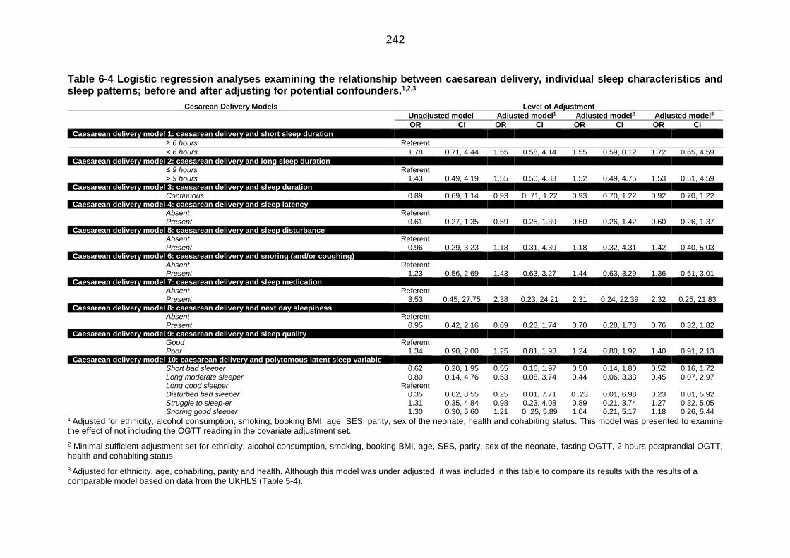
242
Table 6-4 Logistic regression analyses examining the relationship between caesarean delivery, individual sleep characteristics and sleep patterns; before and after adjusting for potential confounders.1,2,3
Cesarean Delivery Models Level of Adjustment
Unadjusted model Adjusted model1 Adjusted model2 Adjusted model3
OR CI OR CI OR CI OR CI
Caesarean delivery model 1: caesarean delivery and short sleep duration
≥ 6 hours Referent
< 6 hours 1.78 0.71, 4.44 1.55 0.58, 4.14 1.55 0.59, 0.12 1.72 0.65, 4.59
Caesarean delivery model 2: caesarean delivery and long sleep duration ≤ 9 hours Referent > 9 hours 1.43 0.49, 4.19 1.55 0.50, 4.83 1.52 0.49, 4.75 1.53 0.51, 4.59 Caesarean delivery model 3: caesarean delivery and sleep duration Continuous 0.89 0.69, 1.14 0.93 0 .71, 1.22 0.93 0.70, 1.22 0.92 0.70, 1.22 Caesarean delivery model 4: caesarean delivery and sleep latency Absent Referent Present 0.61 0.27, 1.35 0.59 0.25, 1.39 0.60 0.26, 1.42 0.60 0.26, 1.37 Caesarean delivery model 5: caesarean delivery and sleep disturbance Absent Referent Present 0.96 0.29, 3.23 1.18 0.31, 4.39 1.18 0.32, 4.31 1.42 0.40, 5.03 Caesarean delivery model 6: caesarean delivery and snoring (and/or coughing) Absent Referent Present 1.23 0.56, 2.69 1.43 0.63, 3.27 1.44 0.63, 3.29 1.36 0.61, 3.01 Caesarean delivery model 7: caesarean delivery and sleep medication Absent Referent Present 3.53 0.45, 27.75 2.38 0.23, 24.21 2.31 0.24, 22.39 2.32 0.25, 21.83 Caesarean delivery model 8: caesarean delivery and next day sleepiness Absent Referent Present 0.95 0.42, 2.16 0.69 0.28, 1.74 0.70 0.28, 1.73 0.76 0.32, 1.82 Caesarean delivery model 9: caesarean delivery and sleep quality Good Referent Poor 1.34 0.90, 2.00 1.25 0.81, 1.93 1.24 0.80, 1.92 1.40 0.91, 2.13 Caesarean delivery model 10: caesarean delivery and polytomous latent sleep variable Short bad sleeper 0.62 0.20, 1.95 0.55 0.16, 1.97 0.50 0.14, 1.80 0.52 0.16, 1.72 Long moderate sleeper 0.80 0.14, 4.76 0.53 0.08, 3.74 0.44 0.06, 3.33 0.45 0.07, 2.97 Long good sleeper Referent Disturbed bad sleeper 0.35 0.02, 8.55 0.25 0.01, 7.71 0 .23 0.01, 6.98 0.23 0.01, 5.92 Struggle to sleep-er 1.31 0.35, 4.84 0.98 0.23, 4.08 0.89 0.21, 3.74 1.27 0.32, 5.05 Snoring good sleeper 1.30 0.30, 5.60 1.21 0 .25, 5.89 1.04 0.21, 5.17 1.18 0.26, 5.44
1 Adjusted for ethnicity, alcohol consumption, smoking, booking BMI, age, SES, parity, sex of the neonate, health and cohabiting status. This model was presented to examine the effect of not including the OGTT reading in the covariate adjustment set.
2 Minimal sufficient adjustment set for ethnicity, alcohol consumption, smoking, booking BMI, age, SES, parity, sex of the neonate, fasting OGTT, 2 hours postprandial OGTT, health and cohabiting status.
3 Adjusted for ethnicity, age, cohabiting, parity and health. Although this model was under adjusted, it was included in this table to compare its results with the results of a comparable model based on data from the UKHLS (Table 5-4).

243
Table 6-5 Logistic regression analyses examining the relationship between preterm delivery, individual sleep characteristics and sleep patterns; before and after adjusting for potential confounders.1,2,3
Preterm Delivery Models Level of Adjustment Unadjusted model Adjusted model1 Adjusted model2 Adjusted model3
OR CI OR CI OR CI OR CI
Preterm delivery model 1: preterm delivery and short sleep duration
≥ 6 hours Referent
< 6 hours 0.24 0.01, 12.59 0.56 0.02, 16.36 0.65 0.03, 16.20 0.40 0 .01, 16.79
Preterm delivery model 2: preterm delivery and long sleep duration ≤ 9 hours Referent > 9 hours 0.14 0.00, 7.20 0.40 0 .02, 10.49 0.45 0.02, 10.04 0.26 0.01, 8.74 Preterm delivery model 3: preterm delivery and sleep duration Continuous 0.53 0.08, 3.41 1.04 0.33, 3.27 1.01 0.35, 2.89 0.82 0.13, 5.01 Preterm delivery model 4: preterm delivery and sleep latency Absent Referent Present 2.29 0.05, 117.53 1.27 0.06, 26.84 1.33 0.07, 24.42 1.78 0.05, 61.60 Preterm delivery model 5: preterm delivery and sleep disturbance Absent Referent Present 8.60 0.16, 452.69 2.78 0.07, 103.73 2.76 0.08, 91.99 5.00 0.09, 268.64 Preterm delivery model 6: preterm delivery and snoring (and/or coughing) Absent Referent Present 0.53 0.01, 27.13 0.76 0.04, 13.62 0 .85 0.05, 14.44 0.63 0 .02, 15.90 Preterm delivery model 7: preterm delivery and sleep medication Absent Referent Present 0.03 0.00, 1.74 0.31 0.00, 46.52 0.30 0.00, 30.49 0.23 0.00, 66.84 Preterm delivery model 8: preterm delivery and next day sleepiness Absent Referent Present 0.48 0.01, 24.87 0.64 0 .02, 17.22 0 .67 0.03, 13.69 0.73 0.02, 27.29 Preterm delivery model 9: preterm delivery and sleep quality Good Referent Poor 0.74 0.10, 5.28 0.88 0.18, 4.25 0.92 0.21, 4.02 0.84 0.12, 5.84 Preterm delivery model 10: preterm delivery and polytomous latent sleep variable Short bad sleeper 2.94 0.06, 153.95 2.05 0.08, 53.49 2.18 0.09, 52.42 2.31 0.05, 98.03 Long moderate sleeper 0.43 0.01, 023.69 0.63 0.01, 35.48 0.66 0.01, 32.17 0.49 0.01, 30.84 Long good sleeper Referent Disturbed bad sleeper 0.14 0.00, 8.95 0.52 0.01, 46.19 0.57 0.01, 45.53 0.38 0.00, 138.74 Struggle to sleep-er 1.11 0.02, 59.20 1.24 0 .03, 53.02 1.39 0.04, 46.08 1.12 0.02, 76.72 Snoring good sleeper 0.71 0.01, 38.48 0.84 0.02, 35.08 0.85 0.02, 30.07 0.79 0.02, 38.40
1 Adjusted for ethnicity, alcohol consumption, smoking, booking BMI, age, SES, parity, sex of the neonate, health and cohabiting status. This model was presented to examine the effect of not including the OGTT reading in the covariate adjustment set.
2 Minimal sufficient adjustment set for ethnicity, alcohol consumption, smoking, booking BMI, age, SES, parity, sex of the neonate, fasting OGTT, 2 hours postprandial OGTT, health and cohabiting status.
3 Adjusted for ethnicity, age, cohabiting, parity and health. Although this model was under-adjusted, it was included in this table to compare its results with the results of a comparable model based on data from the UKHLS (Table 5-4).

244
Table 6-6 Logistic regression analyses examining the relationship between macrosomia, individual sleep characteristics and sleep patterns; before and after adjusting for potential confounders.1,2,3,4
Macrosomia Models Level of Adjustment
Unadjusted model Adjusted model1 Adjusted model2 Adjusted model3
OR CI OR CI OR CI OR CI
Macrosomia model 1: macrosomia and short sleep duration
≥ 6 hours Referent
< 6 hours 0.54 0.09, 3.16 0.80 0.13, 4.91 1.05 0 .17, 6.31 0.54 0.09, 1.97
Macrosomia model 2: macrosomia and long sleep duration ≤ 9 hours Referent > 9 hours 0.99 0.16, 5.97 0.80 0.13, 4.93 0.70 0.10, 4.95 0.99 0.16, 5.97 Macrosomia model 3: macrosomia and sleep duration Continuous 1.34 0.99, 1.97 1.19 0.89, 1.89 1.05 0.70, 1.57 1.34 0.91, 1.97 Macrosomia model 4: macrosomia and sleep latency Absent Referent Present 0.73 0.21, 2.51 0.75 0.21, 2.68 0.78 0.21, 2.85 0.73 0.21, 2.51 Macrosomia model 5: macrosomia and sleep disturbance Absent Referent Present 0.41 0.09, 1.91 0.62 0.12, 3.16 0.61 0.12, 3.11 0.41 0.09, 1.91 Macrosomia model 6: macrosomia and snoring (and/or coughing) Absent Referent Present 0.73 0.20, 2.70 0.64 0.17, 2.41 0.73 0.18, 2.94 0.73 0.20, 2.70 Macrosomia model 7: macrosomia and sleep medication Absent Referent Present 5.97 0.72, 49.82 69.66 0.71, 6871.77 44.05 1.06, 1831.89 5.97 0.72, 49.82 Macrosomia model 8: macrosomia and next day sleepiness Absent Referent Present 1.89 0.57, 6.32 1.86 0.56, 6.22 1.95 0 .57, 6.69 1.89 0.56, 6.32 Macrosomia model 9: macrosomia and sleep quality Good Referent Poor 1.29 0.70, 2.35 1.64 0.83, 3.25 1.77 0.89, 3.55 1.29 0.70, 2.35 Macrosomia model 10: macrosomia and polytomous latent sleep variable Short bad sleeper 0 .60 0.11, 3.12 0.49 0.09, 2.69 0.62 0.10, 3.64 0.60 0.12, 3.12 Long moderate sleeper 1.43 0.16,13.197 0.94 0.09, 10.05 1.59 0.14, 17.88 1.43 0.16, 13.20 Long good sleeper Referent Disturbed bad sleeper 1.24 0.05, 34.20 2.26 0.06, 91.17 1.39 0.14, 13.56 1.24 0.05, 34.20 Struggle to sleep-er 0.53 0.06, 4.50 0.78 0 .09, 6.61 0.78 0.09, 6.61 0.58 0.07, 4.91 Snoring good sleeper 2.28 0.37, 13.99 2.31 0.35, 15.35 3.14 0.41, 24.18 2.28 0.37, 13.99
1 Adjusted for ethnicity, alcohol consumption, smoking, booking BMI, age, SES, parity, sex of the neonate, health and cohabiting status. This model was presented to examine the effect of not including the OGTT reading in the covariate adjustment set.
2 Minimal sufficient adjustment set for ethnicity, alcohol consumption, smoking, booking BMI, age, SES, parity, sex of the neonate, fasting OGTT, 2 hours postprandial OGTT, health and cohabiting status.
3 Adjusted for ethnicity, age, cohabiting, parity and health. Although this model was under adjusted, it was included in this table to compare its results with the results of a comparable model based on data from the UKHLS (Table 5-4).
4 Figures in bold type are statistically significant (p<0.05)

245
Table 6-7 Logistic regression analyses examining the relationship between low birth weight, individual sleep characteristics and sleep patterns;
before and after adjusting for potential confounders.1,2,3
Low Birth Weight Models Level of Adjustment Unadjusted model Adjusted model1 Adjusted model2 Adjusted model3
OR CI OR CI OR CI OR CI
LBW model 1: LBW and short sleep duration
≥ 6 hours Referent
< 6 hours 1.74 0.24, 12.467 1.15 0.14, 9.37 0.62 0.02, 17.51 1.34 0.17, 10.72
LBW model 2: LBW and long sleep duration ≤ 9 hours Referent > 9 hours 0 .76 0.04, 14.88 0.62 0.04, 10.69 0.88 0.04, 21.23 0.44 0.02, 11.88 LBW model 3: LBW and sleep duration Continuous 0.72 0.36, 1.41 0.81 0.45, 1.46 0.78 0.34, 1.84 0.76 0.44, 1.32 LBW model 4: LBW and sleep latency Absent Referent Present 1.06 0.15, 7.44 0.88 0.12, 6.72 1.38 0.12, 16.40 0.96 0.13, 6.97 LBW model 5: LBW and sleep disturbance Absent Referent Present 1.11 0.06, 21.83 0.96 0.04, 21.67 0.22 0.00, 13.01 0.60 0.03, 14.74 LBW model 6: LBW and snoring (and/or coughing) Absent Referent Present 0.78 0.11, 5.47 0.78 0.10, 5.83 1.19 0.10, 14.61 0.83 0.11, 6.21 LBW model 7: LBW and sleep medication Absent Referent Present 3.51 0.16, 78.61 3.73 0.10, 135.34 4.21 0.03, 574.95 10.55 0.24¸469.57 LBW model 8: LBW and next day sleepiness Absent Referent Present 0.22 0.01, 4.21 0.14 0.01, 3.72 0.15 0.01, 3.17 0.29 0.02, 5.39 LBW model 9: LBW and sleep quality Good Referent Poor 1.38 0.56, 3.39 1.17 0.45, 3.03 1.45 0.42, 4.93 1.36 0.53, 3.48 LBW model 10: LBW and polytomous latent sleep variable Short bad sleeper 0.33 0.03, 3.43 0.21 0.01, 8.41 0.18 0.01, 3.78 0.35 0.03, 3.86 Long moderate sleeper 0.73 0.03, 20.18 1.65 0.04, 75.87 1.88 0.03, 136.48 1.51 0.04, 51.75 Long good sleeper Referent Disturbed bad sleeper 2.20 0.07, 70.42 0.01 0.00, 41.61 0.04 0.00, 55.92 1.56 0.03, 71.01 Struggle to sleep-er 0.30 0.01, 7.81 0.14 0.00, 8.98 0.31 0.01, 9.03 0.32 0.01, 8.13 Snoring good sleeper 2.62 0.30, 22.87 4.64 0.32, 68.32 3.84 0.13, 111.36 3.56 0.28, 44.64
1 Adjusted for ethnicity, alcohol consumption, smoking, booking BMI, age, SES, parity, sex of the neonate, health and cohabiting status. This model was presented to examine the effect of not including the OGTT reading in the covariate adjustment set.
2 Minimal sufficient adjustment set for ethnicity, alcohol consumption, smoking, booking BMI, age, SES, parity, sex of the neonate, fasting OGTT, 2 hours postprandial OGTT, health and cohabiting status.
3 Adjusted for ethnicity, age, cohabiting, parity and health. Although this model was under adjusted, it was included in this table to compare its results with the results of a comparable model based on data from the UKHLS (Table 5-4).

246
Table 6-8 Logistic regression analyses examining the relationship between postpartum blood loss, individual sleep characteristics and sleep patterns; before and after adjusting for potential confounders.1,2,3,4
Postpartum Blood Loss (PBL) Models Level of Adjustment
Unadjusted model Adjusted model1 Adjusted model2 Adjusted model3
OR CI OR CI OR CI OR CI
PBL model 1: PBL and short sleep duration
≥ 6 hours Referent
< 6 hours 1.95 0.76, 5.01 1.24 0.40, 3.80 1.32 0.43, 4.05 1.42 0.47, 4.27
PBL model 2: PBL and long sleep duration ≤ 9 hours Referent > 9 hours 3.86 1.31, 11.37 5.61 1.71, 18.34 5.38 1.65, 17.47 5.20 1.66, 16.29 PBL model 3: PBL and sleep duration Continuous 0.98 0.76, 1.27 1.11 0.82, 1.50 1.07 0.80, 1.50 1.09 0.81, 1.47 PBL model 4: PBL and sleep latency Absent Referent Present 0.41 0.18, 0.18 0.50 0.21, 1.22 0.50 0.21, 1.21 0.42 0.18, 1.00 PBL model 5: PBL and sleep disturbance Absent Referent Present 1.20 0.33, 4.37 1.87 0.47, 7.53 1.84 0.46, 7.32 1.26 0.33, 4.81 PBL model 6: PBL and snoring (and/or coughing) Absent Referent Present 1.21 0.54, 2.74 1.21 0.50, 2.92 1.25 0.52, 3.02 1.31 0.55, 3.11 LBW model 7: LBW and sleep medication Absent Referent Present 1.40 0.18, 11.02 0.10 0.01, 1.77 0.11 0.01, 1.93 0.18 0.01, 2.79 PBL model 8: PBL and next day sleepiness Absent Referent Present 1.49 0.66, 3.35 1.25 0.51, 3.10 1.28 0.52, 3.15 1.13 0.47, 2.74 PBL model 9: PBL and sleep quality Good Referent Poor 1.08 0.71, 1.65 0.99 0.62, 1.59 0.99 0.62, 1.58 1.02 0.65, 1.60 PBL model 10: PBL and polytomous latent sleep variable Short bad sleeper 0.33 0.03, 3.43 0.21 0.01, 8.41 0.18 0.01, 3.78 0.35 0.03, 3.86 Long moderate sleeper 0.73 0.03, 20.18 1.65 0.04, 75.87 1.88 0.03, 136.48 1.51 0.04, 51.75 Long good sleeper Referent Disturbed bad sleeper 2.20 0.07, 70.42 0.01 0.00, 41.61 0.04 0.00, 55.92 1.56 0.03, 71.01 Struggle to sleep-er 0.30 0.01, 7.81 0.14 0.00, 8.98 0.31 0.01, 9.03 0.32 0.01, 8.13 Snoring good sleeper 1.69 0.33, 7.58 1.25 0.22, 6.96 1.31 0.23, 7.53 1.51 0.28, 8.22
1 Adjusted for ethnicity, alcohol consumption, smoking, booking BMI, age, SES, parity, sex of the neonate, health and cohabiting status. This model was presented to examine the effect of not including the OGTT reading in the covariate adjustment set.
2 Minimal sufficient adjustment set for ethnicity, alcohol consumption, smoking, booking BMI, age, SES, parity, sex of the neonate, fasting OGTT, 2 hours postprandial OGTT, health and cohabiting status.
3 Adjusted for ethnicity, age, cohabiting, parity and health. Although this model was under-adjusted, it was included in this table to compare its results with the results of a comparable model based on data from the UKHLS (Table 5-4).
4 Figures in bold type are statistically significant (p<0.05).

247
Table 6-9 Logistic regression model ORs that showed the relationship between Apgar score at birth and sleep characteristics; before and after adjusting for potential confounders.1,2,3
Low Birth Weight Models Level of Adjustment Unadjusted model Adjusted model1 Adjusted model2 Adjusted model3
OR CI OR CI OR CI OR CI
LBW model 1: LBW and short sleep duration
≥ 6 hours Referent
< 6 hours 1.72 0.45, 6.53 1.86 0.44, 7.86 1.88 0.41, 8.77 1.88 0.45, 7.88
LBW model 2: LBW and long sleep duration ≤ 9 hours Referent > 9 hours 2.14 0.47, 9.69 2.60 0 .51, 13.09 2.36 0.47, 11.74 2.90 0.59, 14.23 LBW model 3: LBW and sleep duration Continuous 1.19 0.80, 1.76 1.13 0.76, 1.70 1.13 0.74, 1.73 1.19 0.80, 1.78 LBW model 4: LBW and sleep latency Absent Referent Present 1.76 0.41, 7.50 1.58 0.37, 6.85 1.42 0.33, 6.12 1.40 0.33, 5.97 LBW model 5: LBW and sleep disturbance Absent Referent Present 1.10 0.32, 3.77 1.11 0.32, 3.84 1.03 0.29, 3.71 1.07 0.31, 3.68 LBW model 6: LBW and snoring (and/or coughing) Absent Referent Present 1.10 0.32, 3.77 1.11 0.32, 3.84 1.03 0.29, 3.71 1.07 0.31, 3.68 LBW model 7: LBW and sleep medication Absent Referent Present 6.60 0.78, 55.56 19.50 0.61, 623.41 21.75 0.60, 794.74 22.66 0.69, 744.55 LBW model 8: LBW and next day sleepiness Absent Referent Present 0.93 0.25, 3.51 0.68 0.16, 2.93 0.73 0.18, 2.99 0 .63 0.15, 2.63 LBW model 9: LBW and sleep quality Good Referent Poor 1.37 0.73, 2.56 1.41 0.71, 2.79 1.52 0.74, 3.11 1.35 0.70, 2.58 LBW model 10: LBW and polytomous latent sleep variable Short bad sleeper 1.36 0.21, 9.02 0.93 0.13, 6.66 1.03 0.14, 7.69 0.88 0.13, 6.15 Long moderate sleeper 0.73 0.03, 20.18 0.24 0.01, 8.29 0.30 0.01, 11.58 0.37 0.01, 11.96 Long good sleeper Referent Disturbed bad sleeper 2.20 0.07, 70.42 0.89 0.01, 131.81 1.45 0.01, 149.39 0.86 0.01, 53.66 Struggle to sleep-er 1.57 0.19, 13.26 1.21 0.12, 12.18 1.36 0.12, 14.86 1.15 0.13, 10.13 Snoring good sleeper 2.62 0.30, 22.87 1.82 0.19, 17.05 2.08 0.22, 19.87 2.09 0.22, 19.53
1 Adjusted for ethnicity, alcohol consumption, smoking, booking BMI, age, SES, parity, sex of the neonate, health and cohabiting status. This model was presented to examine the effect of not including the OGTT reading in the covariate adjustment set.
2 Minimal sufficient adjustment set for ethnicity, alcohol consumption, smoking, booking BMI, age, SES, parity, sex of the neonate, fasting OGTT, 2 hours postprandial OGTT, health and cohabiting status.
3 Adjusted for ethnicity, age, cohabiting, parity and health. Although this model was under-adjusted, it was included in this table to compare its results with the results of a comparable model based on data from the UKHLS (Table 5-4).

248
Table 6-10 Logistic regression analyses examining the relationship between NICU admission at birth, individual sleep characteristics and sleep patterns; before and after adjusting for potential confounders.1,2,3
NICU Admission Models Level of Adjustment Unadjusted model Adjusted model1 Adjusted model2 Adjusted model3
OR CI OR CI OR CI OR CI
NICU model 1: NICU and short sleep duration
≥ 6 hours Referent
< 6 hours 0.24 0.01, 12.33 0.55 0.02, 14.79 0.61 0.03, 14.95 0 .47 0.01, 20.63
NICU model 2: NICU and long sleep duration
≤ 9 hours Referent > 9 hours 0.13 0.00, 6.87 0.42 0.02, 10.60 0.46 0.02, 10.23 0.24 0.01, 11.22
NICU model 3: NICU and sleep duration
Continuous 0.52 0.09, 3.01 1.06 0.34, 3.27 1.01 0.36, 2.82 1.04 0.19, 5.64
NICU model 4: NICU and sleep latency
Absent Referent Present 2.39 0.05, 122.96 1.28 0.06, 26.86 1.34 0.07, 24.53 1.50 0.04, 52.31
NICU model 5: NICU and sleep disturbance
Absent Referent Present 8.36 0.159, 440.11 2.77 0.08, 99.56 2.78 0.09, 85.13 4.60 0.09, 238.02
NICU model 6: NICU and snoring (and/or coughing)
Absent Referent Present 0.55 0.01, 28.21 0.77 0.04, 14.57 0.80 0.05, 13.33 0.63 0.02, 18.59
NICU model 7: NICU and sleep medication
Absent Referent Present 0.02 0.00, 1.34 0 .26 0.00, 48.92 0.29 0.00, 43.19 0.14 0.00, 16.09
NICU model 8: NICU and next day sleepiness
Absent Referent Present 0.48 0.01, 24.86 0.60 0.03, 14.09 0.63 0.03, 11.68 0.61 0.01, 30.70
NICU model 9: NICU and sleep quality
Good Referent Poor 0.74 0.10, 5.29 0.85 0.19, 3.93 0.90 0.22, 3.79 0.80 0.12, 5.14
NICU model 10: NICU and polytomous latent sleep variable
Short bad sleeper 2.83 0.05, 148.03 1.91 0.07, 49.31 2.15 0.09, 50.78 2.52 0.06, 115.09 Long moderate sleeper 0.43 0.01, 23.69 0.58 0.01, 31.94 0.63 0.01, 28.81 0.42 0.01, 22.67 Long good sleeper Referent Disturbed bad sleeper 0.14 0.00, 8.95 0.46 0.01, 42.13 0.52 0.01, 39.35 0.25 0.00, 16.16 Struggle to sleep-er 1.11 0.02, 59.20 1.14 0.03, 44.84 1.34 0.04, 0 .04 1.13 0.03, 48.31 Snoring good sleeper 0.66 0.01, 35.52 0.73 0.02, 28.88 0.79 0.02, 25.84 0.74 0.02, 36.67
1 Adjusted for ethnicity, alcohol consumption, smoking, booking BMI, age, SES, parity, sex of the neonate, health and cohabiting status. This model was presented to examine the effect of not including the OGTT reading in the covariate adjustment set.
2 Minimal sufficient adjustment set for ethnicity, alcohol consumption, smoking, booking BMI, age, SES, parity, sex of the neonate, fasting OGTT, 2 hours postprandial OGTT, health and cohabiting status.
3 Adjusted for ethnicity, age, cohabiting, parity and health. Although this model was under-adjusted, it was included in this table to compare its results with the results of a comparable model based on data from the UKHLS (Table 5-4).

249
6.5 Discussion
6.5.1 Limitations
The Scott/Ciantar study had a number of limitations, though these should not
diminish the relative importance of this study for enhancing understanding of the
possible association between sleep and pregnancy outcomes in women at risk of
GDM. Quite simply, this is because this remains the only study to-date that has
concentrated on this important high-risk group, whose prevalence appears to be
growing year on year (Farrar et al., 2016).
Nonetheless, since the study only examined women recruited from two clinical
contexts within the same UK-based NHS Trust will inevitably limit the potential
generalisability of the analyses and the external variability of the present chapter’s
findings (Hedt and Pagano, 2011, Bellomo et al., 2009). However, generalisability
might not have been severely compromised given that the Leeds General Infirmary
and St James Hospital are the only two referral hospitals in Leeds that accept
patients from all over Leeds (and further afield) – a geographical area in which
there resides varied multiethnic populations experiencing substantial variation in
socioeconomic status.
A more critical limitation stems from the fact that sleep was measured only once
during the study period. This is likely to have introduced a degree of measurement
error, since night-by-night variation in sleep is common (not least amongst
pregnant women; Al Afif, 2017, Lee, 1998). The risk of measurement error would
have nevertheless been mitigated by the fact that:
I. the questions included in the PSQI were originally (and specifically)
designed to measure sleep over a period of month, and thereby seek to
accommodate a degree of varation/fluctuation in sleep (Carpenter et al.,
1998, Buysse et al., 1989);
II. the relation between unfavourable sleep and the physiological changes
which usually develop in the second trimester of otherwise healthy
pregnancy is likely to be a bidirectional relationship (Wang et al., 2017,
Aurora and Punjabi, 2013, Qiu et al., 2010), though poor sleep was primarily
considered the ‘exposure of interest’ (rather than the ‘outcome of interest’)
in the present thesis and the decision to record sleep during the second
trimester (i.e. before any abnormal physiological/anatomical changes
developed) therefore ensured that ‘sleep’, as measured, could be examined
as the potential cause of (subsequent) pregnancy outcomes.

250
Meanwhile, it is important to consider the potential impact of categorising not only
the individual sleep characteristics and pregnancy outcomes as binary variables,
but also the covariates identified as potential confounders. The decision to reduce
the number of categories in most variables was taken to deal with the
comparatively small number of participants with adequate data to permit their
inclusion in the analyses, merging/reducing categorical data in this way can lead
to or exacerbate cause categorisation error (Vittinghoff et al., 2006).
Somewhat unexpectedly, the criteria used for diagnosing GDM within the UK NHS
were updated in 2015 (National Institute for Clinical Excellence, 2015), just as
recruitment into the Scott/Ciantar study ceased. According to revised criteria,
pregnant women with fasting OGTT results of ≤ 5.6 mmol/l are now to be
diagnosed with GDM (National Institute for Clinical Excellence, 2015). Five women
from the Scott/Ciantar study sample were diagnosed with GDM using these revised
criteria, as one had a fasting OGTT equal to 5.6, and 4 had a fasting 0GTT >5.6.
Fortunately, however, this change in practice should not have radically affected the
results presented in the present chapter, since this focussed on the risk of GDM
and on the OGTT reading itself, rather than on a formal clinical diagnosis of GDM.
Perhaps the most important limitation of the analyses conducted in the present
Chapter relate to the small sample size available (which, as already mentioned,
required most of the variables to be reduced to binary categorical variables in order
to address the possible loss of statistical power; Vittinghoff et al., 2006, Demidenko
, 2006, Freiman et al., 1978). While the sample size proposed in the original
Scott/Ciantar study protocol was already optimistically small, the substantial
proportion of participants lacking data on one or more of the variables of interest
had a substantial impact on the numbers of participants on which the present
chapter’s analyses could be conducted. On the one hand, the completion rates of
sleep questionnaires (85.6%, n=162) and the availability of data from medical
records (71.3%, n=125) both appeared acceptable. However, when combined, the
numbers of participants with complete data fell to almost 50% (57.4 %, n=108),
and thereby substantially reduced the sample of participants with complete data
that could be included in the analyses.
This, substantively reduced sample size inevitably affected the statistical power of
these analyses and will have also increased the risk of type II error (Demidenko,
2006, Freiman et al., 1978). Yet, since this is the first such study of its type
(focusing primarily on women at risk of GDM), and since many of the limited
number of studies in this field had similarly modest sample sizes (the smallest
being n=45, and most being around n=300), the present chapter is still considered

251
to have made a credible and important contribution to this potentially important
topic.
Meanwhile, it is important to stress that the present chapter went to some lengths
to carefully evaluate the potential impact of missingness on the sample and data
available for analysis. In particular it is important to reiterate that missing data were
excluded in two stages. The first was undertaken only after examining the likely
causes of missing data and confirming that this involved the loss of all data due to
missing records or uncompleted sleep questionnaires. The second comprised
carefully examining the distribution of missing data against other variables. This
approach meant that missing data could be excluded after verifying that the
missing data were missing at random. Indeed, this process established that the
pregnancy outcomes of participants with missing sleep data were similar to those
with complete sleep data, and that there did not appear to be any peculiar/unusual
aggregation of outcomes amongst participants with/without missing data. In a
similar fashion, close examination was able to establish that the sleep
characteristics/patterns and sociodemographic and health characteristics of
participants with/without missing data were broadly very similar. In particular, there
was no evidence of ‘dependency’ between the exposures and outcomes, nor were
there abnormal patterns (such as clustering or pairing) in the distribution of missing
data amongst any of the key variables of interest.
Nonetheless, excluding participants with (any) missing data will have inevitably
caused a loss of information, since the rate of missing data varied from 0% to 10%
in the variables of interest. Nonetheless, the majority of participants with (any)
missing data had missing data for more than one variable, indicating either the loss
of entire medical records, non-completion of sleep questionnaires, or both. In these
instances, the modest missingness overlap would have minimized the amount of
information lost and the number of excluded participants. So, even though listwise
deletion might have decreased the statistical power of the analyses and might have
increased the standard errors (SE) of any estimates generated, these estimates
(and their SEs) are likely to have been unbiased, making listwise deletion more
“honest”, and therefore ostensibly superior when compared to many other
conventional methods of estimation (Allison, 2001).
A final limitation worth consideration is that the analyses conducted in the present
chapter might have been at risk of sampling bias, since as women who were
already interested in sleep and/or concerned about their pregnancy were more
likely to have been recruited. At the same time, (more) frequent medical
intervention (particularly for women considered ‘at risk’ of GDM – as all of the

252
participants here were – and those subsequently diagnosed with GDM) might have
influenced the precision of any (preceding) sleep measurements as potential
predictors of poor pregnancy outcome. In other words, for example, this might have
occurred had there been a latent confounder – say ‘anxiety’ – that influenced both
self-reported sleep and the likelihood of medical intervention; or any later
pregnancy complications, such as the early detection of abnormal fundal height
which might have then caused an early induction of labour by the medical team
before the baby grew too large.
6.5.2 Key findings
The key finding of the analyses conducted in the present chapter was that
unfavourable sleep events and less favourable (LCA-derived) sleep patterns were
not always accompanied by an elevated risk of poor pregnancy outcome. Instead,
these were sometimes accompanied by a lower risk of poor outcomes, varying
amongst the different outcomes examined and the different sleep characteristics
observed. However, this key finding was subject to all of the limitations discussed
earlier, which affected both the precision and the quality of this evidence and
limited its generalisability to other populations.
Beyond this key finding, there were several more minor, secondary findings evident
from a closer inspection of the direction and strength of the relationships observed.
In the main, these findings support the theoretical basis of the present thesis,
although the estimates generated had wide 95% confidence intervals which mean
it is not possible to be certain concerning the precision of the interpretations based
thereon. Additionally, as a result of the underpowered analysis, the poor data
quality and the limited generatability of the results, these findings will need to be
confirmed by better quality future studies:
First, the direction and magnitude of the relationship observed between individual
sleep characteristics and pregnancy outcomes were somewhat different to those
observed between LCA-derived sleep patterns and pregnancy outcomes. These
differences might suggest that both of these somewhat different approaches to
defining sleep successfully detected very different aspects of their role in the
development of poor pregnancy outcomes. Additionally, while some of the
individual sleep characteristics displayed similar patterns of relationships with
pregnancy outcomes, this was not the case for the LCA-derived sleep pattern
clusters, each of which had a unique suite of relationships with the pregnancy
outcomes examined. This observation might support the notion that some of the
individual sleep characteristics (e.g. sleep duration and latency) share similar
pathophysiological pathways; whilst each of the LCA-derived sleep patterns had

253
their own unique relationships with pregnancy outcomes, and as such detected
more specific/sensitive ‘net’ effects on potential pathophysiological pathways.
Second, unfavourable sleep characteristics were not always accompanied by an
elevated risk of poor pregnancy outcomes. Indeed, some were occasionally
accompanied by a lower odds of poor pregnancy outcome – something that was
most evident with daytime sleepiness, long moderate sleeper pattern, LBW and
preterm delivery. This finding perhaps suggests that unfavourable/less favourable
sleep may often simply be a symptom of pregnancy and/or the growing foetus
rather than operating as a risk factor for poor pregnancy outcomes. However, this
was not true for caesarean delivery or Apgar score, perhaps because both of these
outcomes are less a reflection of the growing foetus and more a marker for
unfavourable pregnancy complications.
Finally, the use of alternative covariate adjustment sets (to address the uncertainty
as to where, temporally and within the DAG, OGTT results might ‘occur’), was able
to demonstrate that neither the direction nor the magnitude of the relationships
observed differed markedly before or after the adjustment for the OGTT results.
This would have occurred had the ‘direct backdoor path’ between OGTT results
(as a cofounder) and pregnancy outcomes was mediated by subsequent GDM
treatment and glucose monitoring whilst receiving enhanced clinical care. It might
therefore be advisable were future studies to adopt a prospective longitudinal study
design in which there are frequent sleep measurements/assessments and blood
glucose measurements.
Arguably, these findings were inevitably influenced by choices made regarding the
covariates included in each of the regression models. These choices were justified
using the hypothesised DAG, even though this DAG was built on the basis of theory
rather than firm knowledge (and therefore still requires empirical testing). Hence,
changing the covariate adjustment sets would likely alter the estimates generated.
Meanwhile, the referent for sleep used, and the possibility of measurement error
due to the variable nature of sleep (together with the reliance on subjective sleep
measurements), are also likely to have influenced the results obtained. For these
reasons, using a different measurement tool and/or a different sleep referent, might
lead to substantively different findings. Finally, being underpowered and imprecise
the analyses conducted in the present chapter offers less confidence concerning
the magnitude of the estimates generated and the direction of the relationships
observed between sleep and pregnancy outcomes. Nonetheless, given similar
findings were obtained from analyses of the Scott/Ciantar dataset and those based
on the UKHLS dataset might mean that there is a high possibility that these

254
estimates reflected the true direction of the relationships observed between sleep
and pregnancy outcomes (even if their strength might be less certain as a result of
the previously discussed limitations).
6.5.3 Conclusion
The relation between sleep on a range of pregnancy outcomes (some maternal,
some perinatal, and some neonatal) varied according to the type of outcomes and
sleep characteristics/patterns examined. However, unfavourable sleep events and
sleep patterns did not always elevate the odds of poor pregnancy outcomes, and
instead, occasionally lowered these odds. However, these findings lack a sufficient
level of statistical confidence (or functional understanding) and remain somewhat
speculative and imprecise. Importantly, they may reflect the influence of the
medical interventions allocated to women at high risk of developing pregnancy
complications in this group. Nonetheless, since the findings of the present
chapter’s analyses and those based on the UKHLS dataset were very largely the
same regarding the relationship(s) observed between sleep characteristics and
pregnancy outcomes, the replicability of these suggests their findings are likely to
be broadly valid (shared methodological limitations notwithstanding). Indeed, the
very similar findings suggest that there should be less certainty concerning the
(very different) results published elsewhere in the literature, not least given the
concerns raised earlier in the present thesis regarding the apparent evidence of
publication bias. Finally, it is worth adding that the differences between the two
datasets analysed in the present thesis, particularly with respect to the
relationships between latent sleep clusters and pregnancy outcomes, tend to
confirm the thesis’ supposition that sleep clusters are potentially more sensitive to
changes in health (and, possibly GDM treatment) than individual sleep
characteristics; albeit that further research are required to confirm this possibility.
6.5.4 Recommendations
Future studies will be required to address each of the (substantial) limitations
affecting the present chapter’s analyses, so that more precise results and more
certain conclusions can be drawn. Unfortunately, the present chapter’s analyses,
like those using the UKHLS dataset, are the only studies to-date that have used
sleep in the form of a latent sleep variable. For this reason, future studies are
encouraged to adopt the conceptualisation of sleep as a latent variable to generate
and evaluate similar sleep patterns. Additionally, researchers are highly
encouraged to consider the sleep measurement used with great care (and,
potentially more importantly) to choose their ‘normal’ sleep referent category with
great care, since ‘normal’ sleep is likely to represent a broad spectrum of sleep-

255
related phenomena. Until such studies have been performed, understanding of the
relation between sleep and pregnancy outcomes will remain limited, and to a large
extent determined (and undermined) by the quality and quantity of data available,
and each of the key analytical decisions required.
Medical intervention should also be considered with great care when designing any
future studies since such interventions are likely to have a substantial impact on
the results obtained. This will be particularly relevant when sleep is operationalised
as a latent concept; in which multiple measurements of sleep, as well as of any
covariates acting as potential confounders, will help in correctly specifying the
temporal sequence of events and the most appropriate adjustment for any such
interventions. Indeed, although the effect of adjustment for OGTT readings on the
estimates obtained for the relation between sleep and pregnancy outcomes was
minor, appropriate adjustment for OGTT readings will still be required in order to
appropriately reduce any confounding effect associated with medical intervention
(such as the treatment of GDM, prior to the measurement of sleep). Therefore,
perhaps, a better structured study, comparing the effect of sleep on pregnancy
outcomes in women at risk of GDM who either did or did not require and receive
medical intervention, with women who had low risk pregnancies, might highlight
how treatment (before or after the measurement of sleep) might influence any
effect of sleep on pregnancy outcomes.

256
Chapter 7 Discussion
There have been a growing number of studies exploring the potential relationship
between sleep and poor pregnancy outcomes (Ding et al., 2014, Pamidi et
al.,2014, August et al., 2013), especially over the last 10 years (Pelayo and
Dement, 2017). The evidence these studies have generated suggests that there
might well be an association between (what appear to be) ‘less favourable’ sleep
characteristics and a range of pregnancy outcomes (August et al., 2013, Ibrahim
and Foldvary-Schaefer, 2012), However, this evidence is beset by a number of
limitations in relation to both its internal and external validity (Pamidi et al, 2014,
Khan et al, 1999, Lee, 1998). Indeed, the ‘science’ behind the potential
pathophysiological mechanisms through which sleep might affect pregnancy
outcomes is largely built on theoretical extrapolation from studies of non-pregnant
populations, and the likely impact of experimental effects of sleep deprivation on
physiological and metabolic processes during pregnancy (Irish et al., 2015, Ibrahim
and Foldvary-Schaefer, 2012). To some extent this reflects the ethical challenges
of experimentation during pregnancy and the limited number of interventions
capable of improving sleep (Blyton et al, 2013, Reid et al, 2013); and for these
reasons, the bulk of what we know about sleep and pregnancy outcome (as
presented in the literature) is based on the findings of observational studies (Pamidi
et al, 2014, Khan et al, 1999, Lee, 1998).
In these studies, sleep was primarily measured by assessing individual perceptions
of one (or more) sleep characteristics events (e.g. duration, latency and
disturbance), rather than using more objective measures (such as
polysomnography or actigraphy; Silber et al.,2016, Prinz, 2004). The aim of the
present thesis was therefore to carefully evaluate the evidence available in the
literature before identifying (and filling) the key gaps in current knowledge by
examining both a population sample of pregnant women (drawn from the UKHLS
– a representative study of the UK population that offers substantial external
validity) and a clinical population of pregnant women considered to be at elevated
risk of the sorts of metabolic conditions (in this instance, GDM; Sisira et al., 2017,
Bjørn et al., 2007) considered to be particularly susceptible to less favourable
sleep. To address the possibility that any effects of sleep on pregnancy outcomes
might be the result of variation in individual sleep characteristics and/or variation in
sleep ‘patterns’ (i.e. a combination of, and interactions between, individual sleep
characteristics), the operationalization of sleep in the analyses of both samples of
pregnant women compared the relationship between sleep and pregnancy

257
outcomes with sleep defined as multiple individual characteristics and as a single,
more complex, ‘pattern based’ phenomenon.
7.1 Summary of findings and limitations
To achieve the main aim of the thesis, four key questions (KQ) were addressed.
Each question was examined in successive chapters in the present thesis using a
series of studies, each with different designs, data and/or analyses in the following
order;
KQ1: What might be learnt from the methods and findings of previous
empirical studies exploring the relationship between sleep and pregnancy
outcomes regarding: the challenges and potential flaws of such studies; the
strength of the evidence these studies provide; and priorities for
strengthening the evidence generated from existing data sources?
Chapter 3 answered KQ1 using a systematic review and meta-analysis of
published observational studies examining the association between sleep and
pregnancy outcomes. From the systematic review of previous observational
studies (i.e. Chapter 3) it was evident that, few of these studies had examined more
than one (or, at best, a handful) of ‘self-reported’ sleep characteristics; and that
none had sought to examine sleep more ‘holistically’ (i.e. used more than one sleep
characteristic simultaneously to characterise any multifactorial ‘sleep patterns’;
Babson et al., 2012, Casement et al., 2012). There were also a number of potential
biases in many of the analyses reported by these studies, both in terms of sampling
(particularly for some of the rarer pregnancy outcomes), but also in terms of:
sample size/power; multiple testing; and inappropriate covariate adjustment (King
and Zeng, 2001, Khan et al.,1999). There was also some evidence to support the
likelihood of publication bias – the tendency for studies that observe strong and/or
precise associations to be published in comparison to those with null findings
(Song et al., 2013, Rothstein et al., 2006, Easterbrook et al., 1999).
Given these limitations, especially the high likelihood of publication bias, it remains
difficult to conclude with any certainty whether poor pregnancy outcomes are
associated (whether causally, or not) with unfavourable sleep. Indeed, it is entirely
possible (as well as causally plausible) that (some) unfavourable sleep
characteristics are related to a lower risk of some pregnancy outcomes. As such,
these ‘unfavourable’ sleep characteristics might present as symptoms of healthy
pregnancies. This is possible since only a limited range of sleep characteristics
and a limited range of pregnancy outcomes have thus far been adequately
examined (or examined at all) in the literature; while the odds reported in the

258
literature tend to lack precision and the methods involved in generating these seem
affected by a number of potentially problematic errors and flaws. Added to this, the
vast majority of previously published findings based their interpretations on findings
assessed using p-values to examine ‘the’ null hypothesis rather than the
‘alternative’ hypothesis.
KQ2: What, if any, sleep patterns exist amongst the UK population; and are
any of these stable over time and/or associated with socio-demographic and
health characteristics that might provide evidence of reliability and criterion-
based validity?
Chapter 4 answered KQ2 using the UKHLS data set and complex LCA to examine
the presence, temporal stability and criterion based validity of any distinct
multifactorial sleep ‘patterns’. Using latent class analysis of the seven discrete self-
reported sleep characteristics recorded by the UKHLS, the present thesis (in
Chapter 4) was able to identify six distinct ‘sleep patterns’ amongst adults within
the UK population – patterns that were stable over time (i.e. that were present in a
very similar form in two successive Waves of data from the UKHLS) and were
strongly associated with variation in a range of socio-demographic and health
characteristics (these characteristics being chosen on the basis that they were
likely to be determinants and/or consequences of unfavourable sleep; Arber et al.,
2009, Bjørn et al., 2007, Kaneita et al, 2007). The analyses undertaken in this
Chapter (4) found that the associations observed between these six ‘sleep
patterns’ and health and sociodemographic characteristics was more variable than
those observed amongst each of the seven individual sleep characteristics. It
seems likely that these differences indicate that ‘sleep patterns’ are more sensitive
to variation in health and sociodemographic characteristics because they provide
a more holistic measure of sleep overall as compared to each of the individual
sleep characteristics (Alghamdi, 2013, Babson et al., 2012, Casement et al., 2012,
Vermunt, and Magidson, 2004). These findings went some way towards confirming
the plausibility of the present thesis’ so-called ‘hypothesised’ DAG – drawn using
knowledge (and supposition) regarding the timing of measured events/variables to
visualise the likely causal relationships between sleep, pregnancy outcomes and
a range of likely mediators and potential confounders. These findings also helped
justify the use of the ‘long good sleeper’ category as an appropriate referent
category in the analyses undertaken in the two chapters that followed.
For the most part there were only modest concerns regarding the suitability of data
from the UKHLS, albeit that the data on sleep were generated using a subjective
retrospective sleep questionnaire (Abrishami et al, 2010, Coughlin, 1990) based

259
on (but somewhat different to) the validated PSQI (Zhong et al., 2015, Beaudreau
et al., 2012, Buysse et al., 1989), and there were a modest number of participants
with missing data (Little and Rubin, 2014) for one or more of the individual sleep
characteristics and/or sociodemographic and health variables.
KQ3: Is there any evidence that self-reported sleep characteristics predict
subsequent pregnancy outcomes amongst pregnant women who are broadly
representative of the UK population? And to what extent might ‘sleep
patterns’, identified using a range of self-reported sleep characteristics,
predict subsequent pregnancy outcomes amongst them?
Chapter 5 answered KQ3 using the UKHLS population-based dataset and
multivariable regression analyses to assess the relationship between individual
sleep characteristics, LCA-generated sleep patterns and a range of pregnancy
outcomes, before and after adjusting for potential confounders identified using a
directed acyclic graph (DAG).
The six latent sleep patterns identified using LCA on the UKHLS sleep dataset,
together with the 7 individual sleep characteristics measured in the UKHLS sleep
module, were then examined amongst UKHLS participants who had been pregnant
at questionnaire completion during Waves 1 or 4 (see Chapter 5). These measures
of sleep were then examined as potential determinants of a range of self-reported
pregnancy outcomes, using data on the latter provided in the same or subsequent
Waves, and using multivariable logistic regression analyses before and after
adjustment for covariates identified as potential confounders using a directed
acyclic graph (DAG). In general, the results of these analyses provided precious
little evidence of any strong relationships between sleep and poor pregnancy
outcome, regardless of whether these used individual sleep characteristics or LCA-
derived sleep patterns as the exposure of interest. Moreover, where such
relationships were observed, it was clear that unfavourable sleep characteristics
and patterns were not always accompanied by increased odds of poor pregnancy
outcome. Instead, on occasion, less favourable sleep was accompanied with a
lower odds of (some) poor pregnancy outcomes. Meanwhile, the direction and
magnitude of relationships between individual sleep characteristics and pregnancy
outcomes were also somewhat different to that observed for the LCA-derived sleep
patterns – suggesting that individual characteristics and composite patterns
captured different pathways of these relationships or causes to one another
(Buysse, 2014, Alghamdi, 2013, Babson et al., 2012, Casement et al., 2012),
evidence that both may be helpful in better understanding the potential role of sleep
in the development of poor pregnancy outcomes. Unfortunately, these findings may

260
also have been affected by a number of substantive data and sample quality
issues, particularly those stemming from: the paucity of pregnancy outcomes data
(with limited numbers of outcomes reported; and all of these based on maternal
self-reports, which many previous studies have suggested can be rather imprecise;
Schmidt et al., 2015, Herring et al., 2013, Harris et al., 1997); the inclusion of
pregnant women who completed the UKHLS questionnaires at different times
during their pregnancy (i.e. some in the first, some in the second and some in the
third trimester of pregnancy; Al Afif, 2016, Facco et al., 2010); and the use of
multiple testing (of 8 sleep variables and multiple pregnancy outcomes; Sullivan
and Feinn, 2012) and the concomitant risk of type II errors due the underpowered
analyses and inadequate sample size (Freiman et al., 1978).
KQ4: Is there any evidence that self-reported sleep characteristics predict
subsequent pregnancy outcomes amongst pregnant women at increased
risk of developing gestational diabetes? And to what extent might ‘sleep
patterns’, identified using a range of self-reported sleep characteristics,
predict subsequent pregnancy outcomes amongst them?
Chapter 6 answered KQ3 using the Scott/Ciantar study clinical dataset (of women
at elevated risk of GDM) and multivariable regression analyses to assess the
relationship between individual sleep characteristics, LCA-generated sleep
patterns and a range of pregnancy outcomes, before and after adjusting for
potential confounders identified using a directed acyclic graph (DAG). Subsequent
analyses, using similar techniques to those applied to pregnant women from the
UKHLS to women at risk of GDM, nonetheless found very similar results with
regard to unfavourable sleep characteristics (see Chapter 6). However, in this
instance the LCA-derived sleep patterns had very variable relationships with poor
pregnancy outcomes and these were not always accompanied by an elevated risk
of poor pregnancy outcomes. Moreover, there were additional limitations with the
Scott/Ciantar study data which make a direct comparison between analyses of
these data and those of the UKHLS data (in Chapter 5) challenging. In particular
there: were much poorer quality data on covariates acting as potential confounders
(Schmidt et al., 2015, Harris et al., 1997); was a potential risk of sampling bias
(since this study may have only succeeded in recruiting women who were already
interested in sleep and/or were worried about their pregnancy; Hedt and Pagano,
2011); was the likelihood that more frequent medical attention/intervention may
have influenced the precision of any (preceding) sleep measurements as
predictors of (subsequent) poor pregnancy outcomes (if, for example, there had
been a latent confounder – say ‘anxiety’ – that had influenced both self-reported
sleep and the likelihood of medical intervention and its effect[s] on pregnancy

261
outcomes (Crowther et al., 2005, Maxwell et al., 2011). However, while in the
UKHLS analyses (Chapter 5), variation in the gestational age at which sleep data
were recorded was viewed seen as an important potential limitation, in the
Scott/Ciantar study the much tighter period of time over which sleep was recorded
might also be seen as a limitation (not least if this period had been when sleep was
less important or a weaker predictor/determinant of subsequent pregnancy
outcomes; Al Afif , 2016, Facco et al., 2011). In general then, the results of these
analyses revealed no strong associations between sleep characteristics or
patterns and the subsequent odds of poor pregnancy outcome(s) amongst women
zwat increased risk of GDM.
7.2 Evidence of associations between sleep and poor
pregnancy outcomes
Given the limitations of the de novo analyses contained in the present thesis (and
those of previously published studies examined in Chapter 3), perhaps the most
important evidence from Chapters 5 and 6 was that the empirical data did not
always support the claim made in the literature that less favourable sleep was
associated with an increased risk of poor pregnancy outcomes as discussed
comprehensively in Chapter 3. In Chapters 5 and 6 it was clear that while less
favourable sleep predominantly increased the risk of poor pregnancy outcomes
amongst women from the wider UK population or women at risk of GDM; on a
number of occasions less favourable sleep was actually accompanied by a lower
risk of poor pregnancy outcomes. While all of these associations lacked precision
(i.e. had wide confidence intervals, primarily as a result of measurement error and
the modest sample sizes involved; Borenstein et al., 2009, Montori et al., 2004), it
was also clear that whether positive or negative, there usually existed a relationship
of some sort between sleep and pregnancy outcome, and there were very few
occasions where no relationship whatsoever was apparent.
These results contrast quite markedly with those reported in the literature (Pamidi
et al., 2013, Chang et al., 2010, Pien et al., 2004). Indeed there remain, to-date,
limited numbers of studies (particularly considering that some outcomes in relation
to some sleep events have only been examined once thus far; August et al, 2013,
Pamidi et al., 2013); which means that these studies have only examined a limited
range of (clinical and non-clinical) populations (Chang et al., 2010, Pien et al.,
2004), and makes it challenging to compare their findings to those generated in
Chapters 5 and 6, and particularly so for Chapter 6 since many of the studies
reviewed in Chapter 3 had specifically and deliberately excluded pregnancies

262
considered to be ‘high risk’ (including those affected by GDM). And since many of
these studies failed to report many of the more important social and biological
characteristics of their participants (such as socioeconomic status or health
conditions), it remains somewhat unclear whether comparisons between any of
these studies might not be undermined by inter-study heterogeneity (August et al,
2013, Pamidi et al., 2013, Borenstein et al., 2009).
At the same time, the modest number of previous studies, and the fact that most
of these had reported ‘positive’ findings, seems likely to indicate that there may be
numerous unpublished studies (and related datasets; Borenstein et al., 2009,
Dickersin, 1990) which found no evidence of any association between sleep and
pregnancy outcomes, or which might have actually shown the sorts of inverse
relationships between ‘unfavourable sleep’ and ‘good’ pregnancy outcomes that
were observed in Chapters 5 and 6, here (Louis et al., 2012). If, as the published
literature suggests, the overwhelming theoretical hypothesis driving such analyses
is that ‘unfavourable’ sleep characteristics and patterns are likely to pose
substantive risks of ‘poor’ pregnancy outcomes (as a result of the ill-effects of sleep
deprivation on cardio-metabolic health evident in experimental studies of non-
pregnant populations; Cappuccio et al., 2010, Coughlin et al., 2004), then the
tendency for published studies of pregnant women to report ‘positive’ associations
between sleep and pregnancy outcomes, together with the apparent
strength/statistical significance of many of the smaller (and therefore more
underpowered) studies, presents a strong prima facie case for publication bias at
work (see Chapter 3; Rothstein et al., 2006). This impression is further
strengthened by the fact that so few of these published studies recognized and
cited many potential limitations that might have affected their internal validity (again,
see Chapter 3; Grimes and Schulz, 2002, Stroup et al., 2000).
That is not to say that either of the two de novo studies conducted for the present
thesis (i.e. Chapters 5 and 6) were unaffected by potential challenges to their
internal validity - particularly as regards sample size, statistical power, multiple
testing and the risk of type I and type II errors (Demidenko et al., 2006, Grimes and
Schulz, 2002, Freiman et al., 1978). Hence, it cannot be concluded with a
substantive degree of certainty (nor with traditional levels of confidence or
statistical precision) that either of these studies found clear evidence of positive,
inverse or null associations between sleep and pregnancy outcomes. In particular,
these studies do not permit the absence of any association between sleep and
pregnancy outcomes to be rejected with much level of certainty. Yet, in a similar
fashion to that observed in the literature, Chapters 5 and 6 found a number of
statistically significant associations between sleep and poor pregnancy outcomes

263
– associations that are consistent with type I errors, especially were alpha to have
been corrected to account for multiple testing (Bender and Lange, 2001, Benjamini
and Hochberg, 1995, Bonferroni, 1936). Somewhat paradoxically, then, these
‘occasional’, statistically significant (and therefore more precise) findings seem
likely to support the view that the evidence presented in the published literature are
also primarily the result of type I errors (Borenstein et al., 2009, Stroup et al., 2000) .
Such ‘occasional’ findings can be found in many of the studies in which multiple
(ostensibly exploratory) tests were likely to have been applied to more sleep
characteristics than that reported (Keppel and Wickens, 2004, Grove and
Andreasen, 1982) – not least since most of these studies reported that they had
used sleep questionnaires that would have generated data on more than just the
one sleep characteristic on which the published study’s findings hinged.
Nonetheless, and this is perhaps an equally important point, given the findings from
a growing number of published studies, it seems unlikely that there is (as yet)
sufficient evidence to completely reject the possibility or plausibility of an
association between sleep and pregnancy outcomes – though this may, in the main,
simply be the result not only of publication bias, but also the many substantive
limitations of the sampling, sample size, data measurement and analysis
techniques that affect most of these previously published studies (Monroe, 2007,
Grimes and Schulz, 2002, Stroup et al., 2000). However, at best, it seems likely
that any true effect present (such as an increased risk of hypertension-mediated
prematurity or low birth weight, or of obesity and GDM-mediated macrosomia
amongst women with sleep disordered breathing Reutrakul et al., 2013,
Benediktsdottir et al., 2012 Micheli et al., 2011, Qiu et al., 2010) might still be too
modest to detect with any degree of certainty or precision in the sample sizes used
and with such extensive reliance on self-reported (sleep and other) data and data
extracted from clinical records (Maxwell et al., 2011, Fritz and MacKinnon, 2007,
Harris et al., 1997, Coughlin, 1990). Under these circumstances, and for all of these
reasons, the present thesis would argue that previously published studies seem
likely to have exaggerated the strength of any relationships between sleep and
pregnancy outcomes. For this reason alone, better quality studies will be required
to provide the evidence necessary to generate any definitive conclusions regarding
the potential relationship between sleep and pregnancy outcomes.
7.3 Sleep in pregnancy
Several empirical studies, and a wealth of theoretical conjecture, suggest that
sleep is likely to be more ‘problematic’ during pregnancy (Naud et al., 2010) –

264
simply as a result of the effects of the many physical, hormonal and psychological
factors that militate against more favourable sleep (Silber et al., 2016, Sloan, 2008,
Wang et al., 2004). Yet, closer examination of more descriptive studies of sleep in
pregnancy (published elsewhere in the literature) and neither of the two empirical
de novo studies included in the present thesis (Chapters 5 and 6) appear to not
support this. For example, the descriptive summary statistics from published
studies suggest that the reported mean sleep duration of the pregnant women
examined ranged from 6 to 9 hrs/night (Lee and Gay, 2004, Dorheim et al., 2012,
Herring et al., 2014, Wang et al., 2017) – a range that is thought to be within the
‘normal’ length of sleep duration as reviewed in Chapter 3. Likewise, in terms of
overall sleep quality, the majority (60%) of pregnant women in more than one study
reported poor quality PSQI-derived scores (i.e. a PSQI global score of >5; Okun et
al., 2011, Reutrakul et al., 2011), yet when a single question was used to assess
subjective sleep quality only a small minority of pregnant women appear to report
poor sleep quality (2.2%), whilst the remainder tend to report ‘good’ to ‘moderate’
sleep quality (Wang et al., 2017). Such differences in findings generated using two
different tools/approaches to the evaluation of overall sleep quality might indicate:
differential measurement error (Manconi et al, 2010, Elsenbruch et al, 1999); or
differential sensitivity (of the PSQI and individual sleep quality questions) when
detecting sleep problems (Mollayeva et al., 2016). The last of these possibilities
was supported by the comparison of UKHLS sleep module questions and data from
UKHLS participants in the dedicated subsample (who, as part of the methods
development and testing procedures used by the UKHLS, had additionally
completed the PSQI; see Chapter 2 and Appendix), which showed that the PSQI
data failed to identify an important group of women who did not have unfavourable
sleep events.
These summary findings can be interpreted as evidence that the majority of
pregnant women do not appear to display less favourable sleep – an interpretation
that is largely supported by both of the empirical studies presented in this thesis
(Chapters 5 and 6). In these studies, around 70% of pregnant women (from the
UKHLS) and 64% of women at risk of GDM (from the Scott/Ciantar study) reported
that their sleep duration over the month preceding data collection had been within
the reference range (i.e. 6 to 9 hrs/night); while two thirds of pregnant women in
both samples reported ‘good’ sleep quality and an ‘absence’ of disturbed sleep. At
the same time, when the sleep patterns identified on the UKHLS study population
(old and young, male and female, healthy and unhealthy) were applied to the self-
reported sleep characteristics of pregnant women, far more of these women were
found to display long good sleep patterns (12.9%) as compared to other

265
participants in the UKHLS (7.1%). Indeed, the prevalence of LCA-derived good
sleep patterns was even higher amongst women at risk of GDM (15.7 %) than that
observed amongst pregnant women from the wider population (as sampled by the
UKHLS).
While pregnancy is widely considered (and experienced as) a risk factor for
developing some unfavourable sleep events (Ward, B. 2017, Al Afif, 2016);
unfavourable sleep events should not necessarily be considered characteristic of
(all) pregnancy per se, and their presence may (or may not) indicate the existence
of pregnancy complications (Ward, 2017). Comparisons with pre-pregnancy sleep
patterns would be required before drawing such a conclusion (Al Afif, 2016),
although careful consideration should also be given to the possibility that subjective
sleep measurement might (in and of itself) cause substantial measurement errors
which might themselves be susceptible to changes in affect, mood and perception
during pregnancy (Sedov et al., 2017). Of particular relevance in this regard (given
that most previous studies examining the relationship between sleep and
pregnancy examined just one sleep characteristics), using a single sleep
characteristic, be that duration or perceived quality, to argue/demonstrate that
unfavourable sleep is common in pregnancy, would be far from satisfactory (Sedov
et al., 2017, Pamidi et al., 2014). For instance, in Chapter 3, both male and non-
pregnant female UKHLS participants had similar rates of ‘long moderate’ – a
pattern characterised by long hours of sleep, good perceived quality, and an
absence of unfavourable sleep characteristics (except disturbance). Disturbance
was therefore the single individual sleep characteristic that differentiated between
‘long good’ sleepers and ‘long moderate’ sleepers, both of which had a very
different distribution across sociodemographic and health variables. Therefore,
arguing that sleep is ‘worse’ or ‘better’ based solely on the presence (or absence)
of ‘disturbance’ alone might offer a balanced assessment of good vs. bad sleep,
and additional, alternative measures of (other) sleep-related characteristics are
required to do so.
7.4 Sleep as a complex latent variable
Given the likely multifactorial nature of ‘sleep’ and the potential for error were just
one sleep characteristic to be used as a marker/measure thereof, the present
thesis theorised that sleep might be better (and more holistically) described as a
latent variable (Alghamdi et al., 2014, Babson et al., 2012, Casement et al., 2012).
This has not been attempted by any of the previously published studies reviewed
as discussed in ( Chapter 3 and although, on a few occasions, the seven different

266
sleep characteristics available within the UKHLS and Scott/Ciantar study had been
examined by studies exploring the association between sleep and health, these
studies (and others) tended to construct separate theories around the findings
generated for each aspect of sleep and (in the studies reviewed in Chapter 3) how
this might then influence poor pregnancy outcome(s).
In the UKHLS and the Scott/Ciantar study, the 7 sleep individual characteristics,
which were measured using the UKHLS sleep module or PSQI, displayed very
different patterns amongst the study participants to those evident when using the
6 LCA-derived sleep patterns – patterns that differed in both the direction and
magnitude of their relationships with pregnancy outcomes. In particular, while the
strength and precision of the relationships between unfavourable sleep
characteristics and poor pregnancy outcomes varied, each of the 7 individual sleep
characteristics examined were consistently accompanied by an elevated odds of
poor pregnancy outcomes. In contrast, only those pregnant women with sleep
patterns characteristic of LCA-derived clusters 5 and 6 displayed an elevated risk
of poor pregnancy outcomes, and the risk of these was actually lower amongst
women with sleep patterns characterized by clusters 1, 2, 3 and 4 (only one, or
perhaps two, of which might reasonably be considered ‘favourable’ sleep patterns).
Clearly then, amongst pregnant women, the magnitude, precision and direction of
relationships between sleep and pregnancy outcomes was different for individual
sleep characteristics and sleep patterns overall. There are a number of different
possible reasons for this novel and potentially important finding. First, LCA-derived
sleep patterns may suffer from different specification errors to those experienced
by individual sleep characteristics (in particular, that any individual measurement
errors associated by the use of self-reported retrospective questionnaire items
might become conflated when each of the individual characteristics are combined
in the LCA; Collins and Lanza, 2013, Hagenaars et al., 2002). Second,
measurement error might have also been exacerbated by the imposition of rigid
cutoff points to demarcate sleep duration, sleep events or the perception of sleep
quality (Buysse, 2014, Buysse et al., 2008, Buysseet al., 1989), also might be from
relying on recall when collecting birth outcomes data from the UKHLS participants
or during reporting medical data in the medical records by several health personal
(Biemer and Lyberg, 2003, Thiru et al., 2003, Harris et al.,1997). Yet, these
somewhat obvious sources of heterogeneity and error aside, the third possibility is
that the two approaches to characterizing sleep actually measured very different
things – the first measuring separate characteristics/dimensions of sleep; the
second offering a more integrated assessment of sleep which took into account the
inter-dependence and conditional equivalence of different individual sleep

267
characteristics ((Babson et al., 2012, Casement et al., 2012, Wu et al., 2002).
Indeed, the last of these possibilities appears an attractive prospect, considering
so little is still known about the biology of sleep (Prinz, 2004) and what each of the
salient (and therefore measureable/manifest) sleep characteristics might represent
in terms of the physiology of sleep and how these might interact with one another
and with the physiological and biochemical processes involved in the etiology of
disease (Silber et al., 2016). The fact that this, more holistic approach to the
operationalization of ‘sleep’ (i.e. the use of LCA-derived, ostensibly latent sleep
‘patterns’) displayed more variable relationships with both health (in Chapter 4) and
pregnancy outcomes (in Chapters 5 and 6) is prima facie evidence that this was
more sensitive (and therefore a more nuanced assessment of the potential role of
sleep as a consequence, correlate or determinant of poor pregnancy poutcomes)
than the use of individual sleep characteristics (Alghamdi, 2013, Casement et al.,
2012). This is because the more variable relationships observed are likely to be
more useful when trying to identify, design and apply interventions to address ‘less
favourable’ sleep in pregnant women (Vézina-Im et al, 2017, Dorrian and Warland,
2013. Blyton et al, 2013, Kaneita et al., 2005)– essentially knowing to which sleep
pattern women might benefit from thereby concentrating on improving the specific
individual sleep characteristics required to ‘shift’ or ‘nudge’ them into sleep patterns
that are associated with far fewer unfavourable pregnancy outcomes (Vézina-Im
et al., 2017, Irish et al., 2015, Stepanski and Wyatt, 2003. This might prove rather
counter-intuitive given, for example, the finding that long good sleepers (ostensibly
the least unfavourable of the sleep patterns observed) were not those who
displayed the lowest risk of poor pregnancy outcomes.
7.5 Pregnant women at risk of GDM
Women at risk of GDM are considered to (also) be at higher risk of poor pregnancy
outcomes (National Institute For Clinical Excellence, 2015, Wendland et al., 2012)
and of less favourable sleep (Wang et al, 2017, Reutrakul et al, 2013, Qiu et al,
2010) – both, primarily, because many of these women go on to develop
gestational diabetes, a condition that has a well-established increased risk of poor
pregnancy outcomes (particularly macrosomia and caesarean section; National
Institute For Clinical Excellence, 2015, Kamana et al., 2015, Alberico et al., 2014).
Somewhat unsurprisingly, some of the GDM risk factors (notably high BMI) are
also thought to predict poor pregnancy outcomes and unfavourable sleep,
regardless of the development of GDM (Kennelly et al, 2011, Lawrence et al, 2008,
Torloni et al, 2008, Bjørn et al, 2007). However, because blood glucose levels
constitute a continuum (and the cutoff point used to define GDM is arguably

268
somewhat arbitrary; World Health Organization, 2013, Hezelgrave et al, 2012),
women ‘at risk of GDM’ are likely to be at risk of poor pregnancy outcomes and
unfavourable sleep regardless of whether they actually go on to develop GDM.
Amongst the background papers reviewed in Chapter 1, and the specific studies
reviewed in Chapter 3, there was little empirical evidence available concerning the
sleep of pregnant women who were at risk of GDM or who had GDM. Instead, in
most instances, women with GDM were actually excluded from the sample, or
included there in without adjustment for their condition, which made it challenging
to generalise between the results generated from these published studies to the
analyses presented in this thesis’ Chapter 6. These analyses therefore offer novel
insights into the sleep and pregnancy outcomes of women at risk of GDM – insights
that are amenable to comparisons with the analyses presented in Chapter 5 (based
on the population sample of pregnant women from the UKHLS), not least because
both sets of analyses used similarly measured sleep and pregnancy outcome
variables, identical categorisations of these variables, and multivariable logistic
regression analyses informed by comparable causal path diagrams (the directed
acyclic graphs specified in line with the likely temporal sequence of the variables
available for inclusion in the analyses). In the analysis of UKHLS (Chapter 5) and
Scott/Ciantar study data (Chapter 6), the distribution of individual sleep
characteristics and pregnancy outcomes participants was very similar amongst
participants in both samples. However, this was not true with regard to the
distribution of LCA-derived sleep patterns – these patterns displayed very different
distributions in each case.
Since GDM is considered likely to be (potentially causally) linked with unfavourable
sleep events (Wang et al, 2017, Pamidi et al., 2014, Reutrakul et al, 2013, Qiu et
al, 2010), it might have been expected that pregnant women with GDM (or with an
elevated risk of GDM), were more likely to display a higher prevalence of short bad
sleep patterns (Pamidi et al., 2014). Yet in fact, pregnant women from the UKHLS
population sample, most of whom are unlikely to have been at increased risk of
GDM, were even more likely to display short bad sleep patterns, albeit in the
absence of appropriate data on a number of key potential confounders (most
notably BMI; Louis et al, 2012), than those participants in the Scott/Ciantar study.
All potential confounders require careful identification and adjustment when
examining the potential total causal effect of sleep on pregnancy outcomes, and
the lack of data on key covariates likely to have acted as (powerful) potential
confounders is a key weakness and limitation of the analyses present in Chapter
5 (Williamson et al., 2013, McNamee, R. 2003). It is likewise possible that the
paucity of data on gestational age at questionnaire completion in the UKHLS, and

269
the lack of adjustment for gestational age, may have been responsible for the very
different distribution of sleep patterns observed in these participants (from the
UKHLS, who completed the sleep module questionnaire in different trimesters of
pregnancy) and those from the Scott/Ciantar study (who all provided self-reports
of sleep during the second trimester; Mindell et al, 2015, Lee et al, 1998). In effect,
the distribution of LCA-derived sleep patterns of participants in Chapter 5 may have
reflected the patterning of sleep at a very different period in pregnancy to that seen
in Chapter 6. Given the substantial evidence that sleep does vary during the course
of pregnancy (Al Afif, 2016, Mindell et al, 2015), being least ‘favourable’ in the third
trimester, and least ‘unfavourable’ (indeed, somewhat comparable to pre-pregnant
sleep) in the second trimester, with first trimester sleep falling somewhere between
the two (Al Afif, 2016, Mindell et al, 2015, Pien and Schwab, 2004), this factor alone
may suffice to explain the differential distribution of sleep patterns amongst
pregnant women in the UKHLS and Scott/Ciantar studies. Not withstanding the
impact of differences in gestational age at sleep assessment on the sleep patterns
observed in Chapters 5 and 6, it is nonetheless of some interest that the directions
of relationships between individual sleep characteristics and pregnancy outcomes
were very similar in both studies, and that it was only the directions of relationships
between sleep patterns and pregnancy outcomes that differed substantially
between the two groups (just as the distribution of these LCA-derived sleep
patterns had varied between them). It is not immediately clear what might have
made the relationships between sleep patterns and pregnancy outcomes so
different in these two samples (beyond that is, the key difference in population vs.
clinical sample, and [presumed] lower vs. higher risk of GDM; Von Elm et al., 2014,
Monroe, 2007, Stroup et al., 2000). However, these different relationships were all
independent of pre-existing health, suggesting that they were likely to be evidence
of differential affects amongst (ostensibly) ‘healthy’ UKHLS participants and ‘at
higher risk’ Scott/Ciantar participants. Further (and better quality) research, paying
particular attention to greater standardisation in the availability of covariates and/or
the timing of sleep measurement, will be required to confirm that these very
different relationships are indicative of different aetiological pathways linking sleep
to pregnancy outcomes in women at (presumably) negligible risk of GDM (i.e.
participants from the UKHLS) and those at elevated risk of GDM (i.e. the
Scott/Ciantar study participants).
7.6 Recommendations
This thesis purposely appraised evidence available from previously published
studies and evaluated this before designing de novo empirical observational

270
studies that dealt with many of the limitations and flaws evident in the literature.
Although this approach aimed to address weaknesses in the design and analysis
of most previous studies exploring the relationship between sleep and pregnancy
outcomes, there were a number of flaws that could not be addressed (or could only
be incompletely addressed); and for this reason the present thesis would make a
number of recommendations for further research in this area.
7.6.1 Study design
First and foremost, it is recommended that researchers undertake interventional
studies to assess the potential influence of sleep on different samples of pregnant
women experiencing with different metabolic (and other) risk profiles. Such
intervention-based experimental studies would allow researchers to control sleep
independently of health, and thereby assess the independent effect of sleep per
se. Although this might prove difficult to achieve, particularly considering the
vulnerability of both mother and foetus during pregnancy (and the special
protections placed on experimentation with pregnant women), and the absence of
non-pharmacological interventions with proven efficacy for addressing
unfavourable sleep, such studies (not least focussing on the use of continuous
positive airway pressure [CPAP], an effective treatment for sleep disturbed
breathing and obstructive sleep apnoea [OSA]) will nonetheless be crucial for
strengthening evidence of cause-and-effect in this context (Reid et al., 2013,
Guilleminault et al., 2007, Poyares et al., 2007). Unfortunately, the cost of such
studies may prove prohibitive, particularly when studying rare pregnancy outcomes
that might require large numbers of participants to achieve sufficient statistical
power.
In the meantime, a more cost-effective contribution might be made by more, and
better, population level observational studies. To improve the quality of these
(given the many flaws and limitations of the studies examined in Chapter 3), further
consideration should be given to: the prevalence of the pregnancy outcomes
selected; the sample sizes required to meet the needs of statistical analyses (and
the level of precision desired); the measurement of (all known) covariates likely to
act as powerful, potential confounders and/or competing exposures; and (perhaps)
the inclusion of additional sleep measures (beyond the seven ‘core’ sleep
characteristics included in the UKHLS and PSQI instruments), including those
capable of recording objective assessments of sleep from ‘free living’ populations
(such as actigraphy). Careful consideration of (potentially) rare pregnancy
outcomes can help to improve the choice of study design to ensure the design
chosen can accommodate the possibility of rare events.

271
Wherever possible, cross-sectional and retrospective longitudinal designs should
be avoided unless these are the only choice available. This is because, with both
classes of design, the temporal sequence(s) of events can be unclear, making it
very challenging to distinguish between covariates acting as mediators or
confounders. Similarly, careful consideration should also be given when applying
a prospective longitudinal design, especially where there are multiple
measurements of study covariates or when sleep measurements are available in
different gestational trimesters. In both instances, multiple regression models with
different covariate adjustment sets are likely to be required for each sleep
measurement using sets assigned dependent on the time at which covariate
measurements are made and the gestational age at which these and sleep
measurements are recorded.
7.6.2 Sample size
Sample size estimations and power calculations conducted prior to sampling would
help ensure the analyses based thereon have sufficient power to generate
estimates of association with a lower chance of type II error and better precision
than that achieved by many published studies to-date (and the two de novo studies
presented in Chapters 5 and 6 of this thesis). However, not only are sufficient
sample sizes required, but special consideration should also be given to the
variability of important events amongst study participants (i.e. the prevalence of
unfavourable sleep events, poor pregnancy outcomes and/or important study
covariates). With insufficient observations of such events regression models will
struggle to generate clear findings, and even more so with variables that have
multiple categories (Irala et al, 1997). Such concerns can interfere with the
appropriate adjustment for confounding as, for example, was the case in the
present thesis, when women with multiple pregnancies were excluded from the
UKHLS and Scott/Ciantar studies because there were insufficient participants to
estimate (with any degree of precision) the differential effect of sleep on pregnancy
outcomes – an important issue given that multiple pregnancy, in this instance, was
considered an important potential confounder. At the same time, excluding such
participants also undermines the generalisability of the studies, and this is an
important consideration in its own right (Bossuyt et al., 2003).
Unfortunately, small sample sizes together with a limited number of ‘positive’
exposure or outcome ‘events’ might require researchers to reduce the number of
categories examined; and this may also be necessary to optimise the numbers of
confounders that can be included in underpowered samples by collapsing/reducing
the categorisations of these variables in their analytical models. In the present

272
thesis, the latter was a strategy employed in analyses of both the UKHLS and
Scott/Ciantar datasets - polytomous categorical variables being reduced to binary
variables to reduce the numbers of degrees of freedom available in the
multivariable regression models used. Although, reducing the number of the
categories in this way might allow for better confounder adjustment (by increasing
the number of categorical confounders that can be included in models applied to
smaller sized samples), it is also likely to interfere with the precision of the variables
concerned, and thereby the benefit of adjusting for these (Andrich,1995).
7.6.3 Study participants and setting
All researchers need to consider the risk of selection bias when choosing study
participants (Nilsen et al., 2009), especially when recruitment was done within
specified/restrictive contexts (such as hospital wards), rather than contexts in
which a wider distribution of participants is available (e.g., in antenatal care clinics
– since, in this instance, hospitalized pregnant women are much more likely to have
concurrent medical conditions, better access to health care and/or worse sleep, if
only as a result of staying in a working hospital). Additionally, women who are
hospitalized (whether from pregnancy complications or issues with the foetus) are
potentially more likely to participate in the study (due to their elevated risk of poor
pregnancy outcomes), avoid participation (due to anxieties regarding their or their
babies’ health) or provide biased responses (whether deliberately or
subconsciously, to present/understand their circumstances in terms of the issue –
in this instance sleep – placed before them by the researcher).
Most published studies examining sleep and pregnancy outcomes appear to have
used so-called ‘convenience’ samples from just one or two settings, rather than
spelling out a sampling strategy and carefully considering the potential limitations
of the sampling approach taken. For this reason, sampling strategies and
techniques need careful consideration to address potential challenges to both
external and internal validity (Rothwell, 2005; Calder et al., 1982). Furthermore, to
enhance external validity, researchers might benefit from using ‘general population
registries’ (Calder et al., 1982), albeit notwithstanding the importance of being able
to determine the sequences of measured events (particularly when using DAGs to
assist in the identification of confounders and mediators when using cross-
sectional or retrospective longitudinal designs). Either way, researchers need to
carefully focus on inclusion and exclusion criteria applied to their sampling frames
(such as excluding women who cannot speak English or only including
primigravida), as these are central to ensuring the intended generalizability of their
studies’ results (Rothwell, 2005). Descriptions of sampling strategies and

273
inclusion/exclusion criteria rarely were provided in adequate detail by the studies
included in the systematic review conducted for the present thesis, and this,
together with the limited information on the conceptualization and
operationalization of key covariates (such as maternal health conditions and
socioeconomic status), means that it can be extremely challenging to compare and
combine estimates generated by different studies in meta-analyses capable of
assessing the extent (and potential sources of) heterogeneity.
Finally, researchers are advised to study women at risk of poor pregnancy
outcomes (such as women with chronic health conditions, women with multiple
pregnancies and/or obese women), as these groups have thus far been neglected
in the literature to date. This means that, due to their health status and any
concurrent medical interventions, the evidence currently available (i.e., within
published studies) cannot be generalized to them, so further research will be
required.
7.6.4 Measurement of sleep and other covariates
This thesis also highlighted the potential importance of recording sleep on more
than one occasion, and throughout pregnancy - especially for those participants
that suffered late pregnancy events such as GDM or GHTN and/or received
treatment after the measurement of sleep. In future, researchers should be
encouraged to make multiple measurements of sleep to assess (and then make
provision for) its variability, and to take measurements of sleep much closer to the
time of outcome measurement. However, researchers will need to be careful when
assessing relationships that might actually manifest as bidirectional (where sleep
causes poor pregnancy effects that, in turn affect sleep) and, for this reason, avoid
retrospective designs as far as is possible since the likely bidirectionality of sleep-
related causal/correlational pathways make it difficult to address which variables
predicts, and which mediates, the potential effect of each casual pathway. Such
bidirectionality may be a particularly important consideration where researchers
adopt recent advances in the specification of theoretical models (such as DAGs)
prior to statistical analysis, and within the context of sleep and pregnancy
outcomes, it is recommended that researchers carefully consider the gestational
age(s) at which any measurements of sleep are recorded, as this inevitably
determines the likely sequence of events, and thereby the choice of covariate
adjustment sets and the adjustment technique that best suits the analyses (be that
multivariable adjustment, stratification or restriction).
Meanwhile, since this study appears to be the first to treat sleep as a complex
latent variable, it is recommended that future research examining the complex

274
nature and extensive variability of sleep, might want to consider using LCA-derived
‘sleep patterns’ (along the lines of Chapter 4). This may make substantial novel
inroads into our understanding sleep (and its effects) since little is still known about
the true nature (and function[s]) of sleep and, since the LCA-derived sleep patterns
examined in the present study behaved in tantalisingly different ways in a number
of analyses, as compared to analyses of individual sleep characteristics; and these
differences may reflect hitherto hidden processes at play. Additionally, researchers
might benefit from improving the measurement of sleep by developing, validating
and extending the scope of self-reported sleep instruments, and/or augmenting
these with objective measurement tools (if only for use with those aspects of sleep
that are amenable to actigraphic assessment – such as the timing of sleep, sleep
duration, and sleep efficiency; Van Den Berg et al., 2008, Lockley et al., 1999).
Meanwhile, special attention should be given to the referent chosen for binary or
polytomous sleep variables, as results might vary depending on such variables
therein (especially sleep duration). Indeed, in the literature, various studies used a
variety of reference points, although the researchers involved rarely (if ever)
reported why they chose their referent categories or what theories were behind
their choices – and they should be encouraged to disclose these decisions
explicitly. Moreover, because only a limited number of individual sleep
characteristics had been measured/employed in the studies reviewed, more effort
is required to ensure that hitherto under-researched characteristics (such as sleep
position, latency and daytime sleepiness) receive additional attention in the future.
Likewise, attention should be paid to the measurement of study outcomes, as
occasionally, two distinct variables have very similar definitions, though
measurements are taken at very different time points (e.g., maternal BMI upon
booking and at different time points throughout the pregnancy). As a result, the
analysis of these might require different covariate adjustment sets depending on
the time at which the outcome was measured and when it (had) actually/previously
developed. Equally important are the measurement tools used to measure the
specified outcome (e.g., the type of OGTT test used and how post-partum blood
loss was measured/estimated). The categorization of outcome variables also might
affect precision and accuracy (e.g., when elective and emergency caesarean
section were combined in a single variable), as might the time point at which the
outcome was reported/measured (e.g., a premature vs. a term birth weight.
7.6.5 Covariates adjustment and DAG
Standardising the inclusion criteria and measurement protocols for covariates
would also help to tackle some of the key problems faced by the analyses

275
conducted in Chapters 5 (the absence of data on gestational age at questionnaire
completion and on key salient confounders, not least BMI) and 6 (the focus only
on sleep in the second trimester of pregnancy, and the poor quality of many of the
variables extracted from medical records, not least the employment status of the
pregnant woman herself).
As by far, the majority of regression models used by published studies were
inappropriately adjusted (i.e. did not adjust for all measured/measurable
confounders, and/or adjusted for likely mediators), the apparent associations these
analyses report between sleep and pregnancy outcomes might simply be the result
of unadjusted confounding and/or the influence of the reversal paradox. There is
therefore still substantial need for improvements in the specification of multivariable
analytical models, to ensure that such analyses are appropriately adjusted for all
potential/measurable confounders (including, for example, pre-existing maternal
health indicators) and no covariates likely to act as mediators. Improving covariate
Adjustment would, therefore, benefit from each of the following:
I. To reach a minimal, sufficient level of confounder adjustment, it is suggested
that sufficient data be collected (with quality measurements and/or reports)
so that at least one variable from each of the following temporo-functional
groups can be included in the multivariable analyses: age, ethnicity,
socioeconomic status, anthropometric features, mental-health indicators,
maternal-health indicators, previous obstetric history, current maternal
health status, current foetal health status and pre/early-pregnancy maternal
behavioral risks.
II. The temporal sequence of events should be reified as pre-eminent, to allow
for the identification of confounders – an important consideration given that
the direction between sleep and many of the available study covariates is
likely to be (potentially) or temporally bidirectional.
III. The gestational age at which sleep was measured should be carefully
considered when drawing DAGs and, when needed, several DAGs (one for
each gestational age-dependent sleep measurement) might need to be
specified.
IV. It is important to recognize that prospective study designs might require a
different DAG to those developed for retrospective study designs, for each
of which, the sequence of events/measures can vary substantively.
V. When using multiple measurements of sleep, careful consideration
particularly should be given to the specific sequence of events, as multiple

276
DAGs might be required to support the correct specification of several
models (and for each ‘sleep measurement time’, as needed).
VI. Pregnancy outcomes might be better conceptualized as the consequences
of events that interact between them, so that greater attention is given when
including any poor pregnancy outcome as a potential predictor/covariate in
the analytical models used (as is the case, e.g., when caesarean
sectiondelivery as a poor pregnancy outcome might best be conceptualized
as a mediator in the relation between sleep and postpartum hemorrhage).
Finally, it should be remembered that while DAGs are (or at least, can be) useful
visual tools for helping researchers pre-specify their hypothesized casual pathways,
and thereby correctly identify a suitable, minimally sufficient covariate adjustment
set, unless these can include sufficient numbers of confounding covariates in the
subsequent statistical models (and thereby be appropriately adjusted for these
variables), DAGs offer little substantive improvements. Added to that, a poorly
specified DAG that mis-specifies covariates acting as confounders cannot support
appropriately adjusted multivariable analyses. Nonetheless, because DAGs can
be drawn with variables included that have not been measured/recorded (and are,
therefore, ‘latent’ and unavailable for inclusion in any subsequent multivariable
statistical models), DAGs can still be ‘correctly’ specified and yet be of little ultimate
use to the analyses (simply because some/all of the variables identified as potential
confounders have not been measured/recorded; see Chapter 2, Section 2.4.469).
7.6.6 Analysis and data quality
During the systematic review and meta-analysis conducted for the present thesis,
a good many papers were excluded because the analyses only involved
unadjusted t-tests and/or chi square tests. In the future, researchers are urged to
consider the power of multivariable analyses in adjusting for potential confounders
(albeit when supported by well-powered samples capable of sustaining the
inclusion of all necessary confounders in the multivariable statistical models used).
In the present thesis’s primary/de novo analyses, multivariable logistic regression
was chosen as the statistical-analysis tool of choice (primarily to facilitate
comparison). However, several difficulties were faced due to the small sample
sizes available and the limited number of ‘positive’ events among the participants
included in each study’s dataset. Researchers might, therefore, benefit from using
other types of statistical-analysis models capable of estimating risk, despite the
limited number of ‘events’ observed. Researchers also might benefit from using
multilevel analyses to make the most of any multiple measures of sleep and/or
covariates. Indeed, they might even consider using more complicated analyses,

277
such as structural equation models capable of estimating the additive effect of
separate arcs within each causal pathway and including latent variables.
Regardless of the type of analysis chosen, each of the following issues should be
carefully considered, and the results must be interpreted accordingly:
I. Power should be examined (preferably a priori), as many of the published
estimates lack precision and were prone to type II error (Dziak et al., 2014,
Freiman et al., 1978).
II. The sample size available is also of substantial importance when adjusting
for confounders or running complicated analyses, since smaller
(underpowered) sample sizes can undermine model stability, as well as
the models’ capacity to include all necessary potential confounders
(Vittinghoff et al., 2006)
III. When multiple-theory testing is conducted, the p-value used (if it is used)
might require correction before interpretation, given the increased risk of
type I error (Bender and Lange, 2001).
Finally, more effort should be made to produce data of better quality (concerning
not only the accuracy, but also the precision and completeness of the data), and
to report data-quality limitations when publishing study findings. Although this
thesis failed to use multiple imputation due to computing difficulties and a shortage
of appropriate covariates, researchers might want to consider imputing any missing
data using multiple imputation (to enhance the completeness of their data) and/or
carefully investigating the missingness pattern as needed (before dealing with their
missing data) (Van Burren, 2012; Rubin, 1996). However, researchers should do
their best to prevent losing data at the point of collection, and, in the case of
extracting data from medical records (in which the quality of data might be varied
and vulnerable to missingness), researchers would benefit from planning any
potential imputation before extracting their data, if only to ensure that they utilize
sufficient numbers of participants (and data on a sufficient range of covariates
required for imputation) to run such imputations successfully.
7.7 Contribution to the Knowledge
On 21 November 2017, while watching the ITV lunchtime news, I was surprised to
hear about a health campaign to prevent still-births by educating pregnant women
not to sleep on their backs (Lunchtime News, 2017), a recommendation based on
a single study that recently had been conducted in the UK that found a two-fold
elevated risk of still-births amongst pregnant women from sleeping on their back
(Heazell et al., 2017). Unfortunately, this study, like so many other studies on sleep

278
and pregnancy outcomes, suffered multiple flaws that are likely to have interfered
with the quality of the evidence collected. Nevertheless, perhaps the single largest
contribution made by the present thesis was in highlighting the uncertainty of the
evidence currently available and pointing out that more studies of (far) better quality
are needed before we can be certain about the nature of the relationship between
sleep and poor-pregnancy outcomes (as well as before designing interventions to
prevent poor-pregnancy outcomes by altering pregnant women’s sleep habits).
Indeed, contrary to the published literature, the present thesis found evidence to
suggest that (some) unfavourable sleep events might not always be accompanied
by poor pregnancy outcomes, but that occasionally, they might simply be
considered symptoms of healthy pregnancy. While these findings were (like others
in the underpowered analyses undertaken for this thesis) uncertain and lacked
precision, the findings were evident in analyses of both the UKHLS pregnancy
study and Scott/Ciantar study, even though these two studies comprised data from
two very different populations experiencing very different levels of medical
intervention. This finding supported the thesis’s claim about the possibility of
publication bias within the current evidence and that researchers might have
published their results based on p-value, which examined the null hypothesis,
rather than the other hypotheses, one of which might suggest that sleep sometimes
was accompanied by a lower risk of pregnancy outcomes, as this thesis proposed.
Regarding a sleep definition, this thesis was the first to examine sleep in pregnancy
as a latent variable, and interestingly, each pattern of sleep predicted poor
pregnancy outcomes differently and independently of the other patterns,
suggesting that little is known still about sleep and that further effort should be
made to approach sleep holistically. Conveniently, this thesis created an algorithm
to generate the six latent sleep patterns using participants’ responses to the seven
sleep questions presented in the UKHLS, then made the algorithm available for
interested researchers to use in their own future analyses. Additionally, this thesis
highlighted the importance of carefully choosing the reference point of sleep and
the time of sleep measurements (i.e. gestational age) as both might alter the results.
Finally, this thesis was the first to examine sleep in relation to pregnancy outcomes
in a high-risk population. This aspect made our thesis valuable for future
researchers, who might develop a similar interest in this field, especially after
knowing that this thesis highlighted most possible limitations and suggested
several comprehensive recommendations to avoid these limitations, which
concerned the study design, covariate adjustment, analytical models and data
quality. Since this thesis proudly covered many sleep events and poor-pregnancy

279
outcomes, either by applying thoughtful systematic review and meta-analysis
research, or by applying several de novo empirical studies, it might be considered
a rich source of knowledge for future research, especially considering that this
thesis emphasized that some unfavourable sleep events might be symptoms of a
healthy progressing pregnancy.
7.8 Future steps and knowledge sharing/dissemination
At the end of this thesis, we had more questions than answers, so we hope to
initiate an ‘ideal’ study that might answer the uncertainty of the relation between
sleep and pregnancy outcomes, although one study cannot answer that, as
multiple, high-quality studies are needed before reaching certainty. This proposed
study should be free of the flaws and limitations of this thesis, such as being large
enough to be well-powered and having a prospective longitudinal (preferably
interventional) design that has multiple measurements of sleep and pregnancy
outcomes over several pregnancy trimesters, although we suggest that the first
sleep measurement should be taken before pregnancy to establish a baseline
measurement. We proposed using different measurement tools to assess sleep to
better gauge accuracy in sleep measurements (i.e., subjective, as well as objective,
sleep measurements depending on the nature of the sleep characteristics, e.g.,
subjective measurement for quality and objective measurement for duration).
Additionally, there should be a sufficient number of clinical and sociodemographic
covariates with known temporal sequences to adjust for in the analysis, preferably
multilevel to spot variations in sleep over various gestational ages. However, this
proposed study might require long durations and plenty of resources, but as the
Scott/Ciantar study started as a pilot study, we might suggest improvements and
enhancements in their study for future research.
In Chapter 3, our systematic review and meta-analysis critically appraised the
quality of evidence presented in the literature, highlighted possible limitations in the
current knowledge about sleep and pregnancy outcomes and (cautiously)
suggested the possibility of publication bias for the first time in this field. Therefore,
we aim to publish our review results (while considering the possible limitations) to
reflect the uncertainty in current evidence and encourage further and better
research in this area.
In Chapter 4, we generated six latent sleep patterns and suggested that they were
valid and stable by running several investigatory sub-studies. Later, we aim to
make these generated latent-sleep cluster membership algorithms available to

280
other researchers to use in their own research, as this might encourage them to
adopt (conveniently) the complex concept of latent sleep in their future analysis.
In Chapter 5, we examined the relationship between sleep and pregnancy
outcomes, but our analyses were limited by data-quality issues and a lack of
important pregnancy-related variables. Thus, the next step will be to contact the
UKHLS research group to draw their attention toward the importance of reporting
the gestational age when sleep is measured. Additionally, we would like to draw
their attention to the importance of reporting temporal sequences of events related
to pregnancy and (perhaps) suggest including further data in their pregnancy
module about previous obstetric events, pre-pregnancy weight (or weight gain
before sleep measurement), and current maternal and/or foetal complications.
Finally, we hope to highlight the difficulties in imputing UKHLS data using multiple
imputation (due to the considerable number of categories and the large number of
participants), as well as advise them on the crucial importance of multiple
imputation (especially when using a smaller sub-sample from the UKHLS main
dataset), as the amount of missing data reduced the power of our UKHLS
pregnancy study dramatically.
In Chapter 6, we examined the relationship between sleep and pregnancy
outcomes in women at risk of GDM using the Scott/Ciantar study. During data
extraction from medical records, accessing requested medical files was very
difficult as well as time consuming, and a significant effort was made to trace
missing charts. Therefore, we plan to contact the research authority in the Leeds
NHS Trust to highlight the difficulties that researchers experienced trying to access
data and (perhaps) to suggest creating an electronic database that might facilitate
easy data access. Additionally, the quality of data presented in the medical records
was lacking; thus, an effort will be made to contact health personnel, including Dr.
Scott and Dr. Ciantar, regarding data quality to highlight the limitations in some
variables. Finally, we aim to publish some methodological papers about strategies
in data collection and suggest some methods to improve the quality of pregnancy-
related data (such as collecting data from notes made during multiple visits to
examine data consistency).
Last, but definitely not least, we aim to publish the results of the UKHLS pregnancy
study and Scott/Ciantar study to share the fact that an alternative hypothesis exists
and that researchers should make more of an effort to examine this hypothesis,
rather than focus on rejecting the null hypothesis.

281
7.9 Conclusion
In conclusion, the present thesis found that there is only weak evidence of a
relationship between unfavourable sleep events and poor pregnancy outcomes,
and that all of these results lack precisions. Moreover, less favourable sleep is not
always accompanied with an increased risk of poor pregnancy outcomes and, in
some instances less favourable sleep has a modestly strong relation with good
pregnancy outcomes. Further research using better (larger) samples, better
(quality) data, and better (specified) analyses is therefore required in this area
before it will be possible to achieve a degree of certainty and confidence regarding
the potential role that sleep might play in the aetiology of poor pregnancy
outcomes. Such research seems likely to demonstrate that many of the claims and
much of the hyperbole surrounding the (apparent) association between sleep and
pregnancy outcomes simply reflects publication bias.

282
Chapter 8 Appendix
The present chapter contains substantial additional detail relevant to each
of the preceding chapters
8.1 Methodology
8.1.1 Pittsburgh sleep Quality index (Buysse et al., 1989)
Instructions: The following questions relate to your usual sleep habits
during the past month only. Your answers should indicate the most
accurate reply for the majority of days and nights in the past month.
Please answer all questions. During the past month,
1. When have you usually gone to bed? ______________
2. How long (in minutes) has it taken you to fall asleep each night?
______________
3. When have you usually gotten up in the morning? ______________
4. How many hours of actual sleep do you get at night? (This may be
different than the number of hours you spend in bed) ______________
Not during the past month
Less than Once
a week
Once or
twice a week
Three or more
times a week
5-During the past month, how often have you had rouble sleeping because you…
a. Cannot get to sleep within 30 minutes
() () () ()
b. Wake up in the middle of the night or early morning
() () () ()
c. Have to get up to use the bathroom
() () () ()
d. Cannot breathe comfortably () () () ()
e. Cough or snore loudly () () () ()

283
Not during the past month
Less than Once
a week
Once or
twice a week
Three or more
times a week
f. Feel too cold () () () ()
g. Feel too hot () () () ()
h. Have bad dreams () () () ()
i. Have pain () () () ()
j. Other reason(s), please describe, including how often you have had trouble sleeping because of this reason(s):
() () () ()
6. During the past month, how often have you taken medicine (prescribed or “over the counter”) to help you sleep?
() () () ()
7. During the past month, how often have you had trouble staying awake while driving, eating meals, or engaging in social activity?
() () () ()
8. During the past month, how much of a problem has it been for you to keep up enthusiasm to get things done?
() () () ()
9. During the past month, how would you rate your sleep quality overall?
Very
good
Fairly
good
Very bad
Fairly
bad

284
8.1.2 Comparing the UKHLS sleep module questions with the PSQI
sub-study
8.1.2.1 Rationale
The UKHLS sleep module could be considered a short version of the PSQI, as it
consists of questions presented in the PSQI. However, it is unknown how valid this
might be. This issue will be addressed in the following section of the Appendix
because this was not the main purpose of this thesis (although it was an important
step in using the UKHLS sleep module questions to measure sleep).
8.1.2.2 Method
8.1.2.2.1 Data source
The UKHLS innovation panel households were selected by postcodes using a
complex, multistage, random selection process. The innovation panel was
designed to conduct methods testing for the mainstage component of the study,
and involved a group of households randomly assigned to receive an alternative
(test) survey instrument or procedure. For the comparison of UKHLS sleep module
questions and those from the PSQI, the data collection method and data content
were similar to those of the mainstage study discussed previously. Sleep data were
available in three Waves; Waves 1, 2 and 3. The first wave of the innovation panel
started 12 months prior to the first wave of the mainstage study. The third Wave
was completed in 2010 and the fourth wave in 2011 (Figure 8-1).
Figure 8-1 Waves of the Innovation panel data publication years and the sleep measurement tools used in the Waves of interest

285
8.1.2.2.2 Participants
The participants included in this comparison study were all of the adult males and
females (age > 16 years) who participated in the three Waves (Waves 1, 3 and 4)
of the UKHLS innovation panel , and had therefore completed each of the sleep
modules and had complete data from these (n= 733; Figure 8-2; University of
Essex; Institute for Social and Economic Research, 2016).
Figure 8-2 Flow chart showing the included and excluded participants in the UKHLS sleep module/PSQI comparison study
8.1.2.2.3 Sleep measurement
Sleep was measured three times during the first four Waves. The first
measurement made use of the PSQI during Wave 1 of the panel; the second and
third measurements used the UKHLS sleep module questions, during Waves 3 and
4 (Figure 8-1).
As summarised in Table 8-1, each question in the UKHLS sleep module was
similar to a question in one of the components of the PSQI. Therefore, in the
comparison study, each question in the UKHLS sleep module was compared to its
equivalent component in the PSQI. However, there was no question in the UKHLS
sleep module to represent sleep efficiency, and there was no equivalent
component in the PSQI to evaluate sleep disordered breathing. For the
comparison, it was therefore necessary to simulate a new component from
questions available within the PSQI to identify participants with possible sleep-
related breathing disorders. This was constructed this using two questions
extracted from the ‘sleep disturbance’ component of the PSQI. These concerned

286
trouble with sleeping due to coughing or snoring loudly, and trouble with sleeping
due to an inability to breathe comfortably. Scoring was undertaken in a similar
process to that used in the original scoring of the next-day dysfunction and latency
components of the PSQI (Table 8-1). In regards to the efficiency component in the
PSQI, since sleep efficiency was not included in the LCAs conducted in Chapter 4
of the present thesis (since this was not available in the UKHLS sleep module) and
it was not possible to construct a similar component using sleep questions present
in the UKHLS sleep module.
During the LCA stage, the response categories of both the PSQI questionnaire and
the UKHLS sleep module questions were standardised. Following the PSQI
scoring guidelines, sleep duration was categorised as ≥ 7 hours, ≥ 6 hours but < 7
hours, ≥ 5 hours but < 6 hours, and < 5 hours. The following responses were then
combined and renamed as “less than three times a week,” “less than once a week”
and “once or twice a week.” By choosing this frequency of events, the intention
was to match these to the International Statistical Classification of Diseases (ICD
10) diagnostic frequency for insomnia, which comprises: the frequency of an event
of more than three times per week or at least once a month (World Organization
Health, 1992). Quality was coded as “good” if the response to that question was
good or fairly good, and “bad” if the response was bad or fairly bad.
Table 8-1 Questions present in the PSQI, and the corresponding questions present in the UKHLS sleep module
Sleep PSQI Sleep Questions UKHLS sleep module Questions
Duration During the last month How many hours of actual sleep did you usually get at night? (This may be different than the number of hours you spend in bed)
How many hours of actual sleep did you usually get at night? (This may be different than the number of hours you spend in bed)
Coding Before After Before After Hours of sleep per
night (hours: min)
> 7 hours < 7 hours and > 6 hours < 6 hours and > 5hours < 5 hours
Hours of sleep per night (hours: min)
> 7 hours < 7 hours and > 6 hours < 6 hours and > 5hours < 5 hours
Efficiency 1. When have you usually gone to bed? 2. How long (in minutes) has it taken you to fall asleep each night? 3. When have you usually gotten up in the morning? 4. How many hours of actual sleep do you get at night?
Was not measured in the module
Coding Before After
Efficiency=number of hour slept/number of
Did not include in the LCA

287
Sleep PSQI Sleep Questions UKHLS sleep module Questions
hours spent in bed x 100= % >85%=0 75-84%=1 65-74%=2 <65%=3
Disturbance During the past month, how often have you had trouble sleeping because you…… 1- Wake up in the middle of the night or
early in the morning? 2- Have to get up to use the bathroom? 3- Cannot breathe comfortably? 4- Cough or snore loudly? 5- Feel too cold? 6- Feel too hot? 7- Have bad dreams? 8- Have pain? 9- For some other reason?
Responses: a) Not during the past month (0
point) b) Less than once a week (1 point) c) Once or twice a week (2 points) d) Three or more times a week (3
points) e) More than once most night (4
points)
During the past month, how often have you had trouble sleeping because you…… Wake up in the middle of the night or early in the morning?
Coding Before After Before After Sum of points of
each question: Total =0, disturbance =0 Total =≥ 1 and ≤9, disturbance= 1 Total >9 and ≤ 18, disturbance= 2 Total>18, disturbance =3
The total was categorized into three instead of four: 0=0 1 or 2 =1 3=2
a) Not during the past month
b) Less than once a week
c) Once or twice a week
d) Three or more times a week
e) More than once most night
a) Not during the past month
b) Less than twice a week
c) Three or more times a week
Latency 1-During the past month, how often
have you had trouble sleeping because you…… 2-Cannot get to sleep within 30 min.? How long did it take you to fall asleep each night?
a) Not during the past month (0
point)
b) Less than once a week (1 point)
c) Once or twice a week (2 points)
d) Three or more times a week (3
points)
During the past month, how often have you had trouble sleeping because you…… Cannot get to sleep within 30 min.?

288
Sleep PSQI Sleep Questions UKHLS sleep module Questions
e) More than once most night (4
points)
Coding Before After Before After STEP 1
Q1 score: > 0 and < 15=0 > 15 and < 30=1 > 30 and < 60=2 > 60=3 STEP2 Sum of Q1+Q2 0=0 > 1 and < 2=1 > 3 and < 4=2 > 5 and < 6 =3
The total was categorized into three instead of four: 0=0 1 or 2 =1 3=2
a) Not during the past month
b) Less than once a week
c) Once or twice a week
d) Three or more times a week
e) More than once most night
a) Not during the past month
b) Less than twice a week
c) Three or more times a week
Breathing Sleep disorders
During the past month, how often have you had trouble sleeping because you…… Cough or snore loudly? Cannot breathe comfortably?
During the past month, how often have you had trouble sleeping because you…… Cough or snore loudly?
Coding Before After Before After Sum of Q1+Q2
0=0 > 1 and < 2=1 > 3 and < 4=2 > 5 and < 6 =3
The total was categorized into three instead of four: 0=0 1 or 2 =1 3=2
a) Not during the past month
b) Less than once a week
c) Once or twice a week
d) Three or more times a week
e) More than once most night
a) Not during the past month
b) Less than twice a week
c) Three or more times a week
Medication During the past month, how often
have you taken medicine (prescribe or “over the counter”) to help you sleep?
During the past month, how often have you taken medicine (prescribe or “over the counter”) to help you sleep?
Coding Before After Before After a) Not during the
past month b) Less than
once a week c) Once or twice
a week d) Three or more
times a week
a) Not during the past month
b) Less than twice a week
c) Three or more times a week
a) Not during the past month
b) Less than once a week
c) Once or twice a week
d) Three or more times a week
a) Not during the past month
b) Less than twice a week
c) Three or more times a week

289
Sleep PSQI Sleep Questions UKHLS sleep module Questions
Sleepiness During the past month, how often have you had trouble staying awake while driving, eating meals or engaging in social activity? During the past month, how much of a problem has it been for you to keep up enthusiasm to get things?
During the past month, how often have you had trouble staying awake while driving, eating meals or engaging in social activity?
Coding Before After Before After Sum of Q1+Q2
0=0 > 1 and < 2=1 > 3 and < 4=2 > 5 and < 6 =3
The total was categorized into three instead of four: 0=0 1 or 2 =1 3=2
a) Not during the past month
b) Less than once a week
c) Once or twice a week
d) Three or more times a week
a) Not during the past month
b) Less than twice a week
c) Three or more times a week
Subjective sleep quality
During the past month, how would you rate your sleep quality overall?
During the past month, how would you rate your sleep quality overall?
Coding Before After Before After a) Very good
b) Fairly good c) Fairly bad d) Very bad
a) Good b) Bad
a) Very good b) Fairly good c) Fairly bad d) Very bad
a) Good b) Bad
8.1.2.3 Analysis
First, descriptive frequency and percentage tables were used to describe the
sociodemographic features and sleep characteristics of the innovation panel
participants. In addition, missing data were examined for any pattern of
missingness before excluding these prior to the analysis.
Second, the UKHLS sleep module and PSQI were each examined for internal
consistency using Cronbach’s alpha (Cronbach, 1951). Cronbach’s alpha is a
widely used test to measure the internal consistency of such questionnaire. The
magnitude of Cronbach’s alpha increases as the correlation between questionnaire
items increases, since the questionnaire items measure the same construct.
Third, the Spearman correlation, which is a non-parametric test capable of
assessing the monotonic relation between two ranked variables (Spearman, 1904),
was chosen to examine the association between the PSQI questions and sleep
component scores, as both of these were ranked variables. For the questions in
the UKHLS sleep module to be substituted for the relevant PSQI components, they

290
should have the highest correlation with each of the relevant components and
should have a low correlation with all other components.
Later, LCAs were run using Wave 1 sleep data measured by the PSQI and Wave
3 sleep data measured using the UKHLS sleep module questions, separately. In
addition, these LCAs were applied twice using Wave 1 sleep data measured using
the PSQI and that before and after modifying the sleep disturbance score. These
LCAs were used to determine if the UKHLS sleep module and PSQI would
differentiate the group of participants who were free of unfavourable sleep events
from those who had them, and would describe similar numbers of clusters with a
variety of different levels of severity.
Finally, the longitudinal validity of the UKHLS sleep module or the stability of sleep
patterns over time was examined by repeating the LCA over Waves 3 and 4.
Unfortunately, it was not possible to measure the longitudinal validity of the PSQI
using LCA to compare this with the UKHLS sleep module, since the PSQI was
used only once in Wave 1 of the innovation panel.
The Bayesian information criterion (BIC) was used to compare LCA models, with
the model having with the lowest BIC considered to be the best-fitting model. All
LCAs were performed using Latent Gold 4.5 software (Statistical Innovations Inc.,
2009).
8.1.2.4 Results
8.1.2.4.1 Sociodemographic features
As seen in Table 8-2, the distribution of the participants’ sociodemographic
characteristics among each of the three Waves were similar. The majority of
participants were females, almost 54% of whom were in all three Waves. Nearly
43% of the participants were in their forties or fifties. Around 40% had a GCSE-
level of education or lower, and around 96% were white. In regard to economic
status, nearly 62% of the participants were working at the time of the interview.
Sleep characteristics
Table 8-3 summaries the distribution of sleep characteristics among each of the
three Waves. Sleep duration, medication use and sleep quality shared a similar
distribution amongst all three Waves. More than half of the participants had a sleep
duration longer, or equal, to 7 hours per day. More than 80% of the participants in
the three Waves did not use medication and reported good sleep quality.

291
However, sleep latency, disturbance and snoring were substantially different in
Wave 1, as these were measured using the PSQI component score instead of a
single question. In Wave 1, around 56% of the participants reported non-habitual
sleep latency using the PSQI latency component, compared to 42% in Wave 3 and
45% in Wave 4 (the latter using the UKHLS sleep module questions). When using
the PSQI component to measure disturbance in Wave 1, around 90% of the
participants reported non-habitual disturbance, compared to 42% in Waves 3 and
4 (when the UKHLS sleep module was used). Meanwhile, using the UKHLS sleep
module to measure snoring detected around a quarter of the participants as having
non-habitual snoring, while using the PSQI component score resulted in 34% with
non-habitual snoring (Table 8-3). Missing data were excluded prior to the analysis
after confirming that the distribution of missing data was “missing at random”.
Missing at random means that there was no clustering of missing data amongst
participants with certain sociodemographic features, and no dependency on
missing data between any specific variables, such as age and missing data on
sleep items.

292
Table 8-2 Sociodemographic features of subjects who participated in w1, w3 and w4 of UKHLS innovation panel
Wave 1 Wave 3 Wave 4
All participants Matched participants with complete sleep
data
All participants Matched participants with complete sleep
data
All participants Matched participants sleep with
complete data
n=2,568 % n=733 % n=1,756 n=733 % n=2,385 % n=733 % Gender Male 1,186 46.18 331 45.16 806 45.9 331 45.16 1,081 45.32 331 45.16 Female 1,382 53.82 402 54.84 950 54.1 402 54.84 1,304 54.68 402 54.84 Missing 0 0 0 0 0 0 0 0 0 0 0 0 Age ≤19 years 139 5.41 18 2.46 94 5.35 8 1.09 149 6.25 5 0.68
20-39years 732 28.5 206 28.1 439 25 176 24.01 627 26.29 166 22.65 40-59 years 918 35.75 312 42.56 645 36.73 320 43.66 892 37.4 321 43.79 ≥ 60 years 779 30.33 197 26.88 578 32.92 229 31.24 717 30.06 241 32.88 Missing 0 0 0 0 0 0 0 0 0 0 0 0
Education A level and above 985 38.36 336 45.84 721 41.06 349 47.61 1,145 48.01 353 48.16 GCSE level and others 1,080 42.06 307 41.88 705 40.15 301 41.06 909 38.11 299 40.79 Missing 503 19.59 0 0 330 18.79 83 11.32 331 13.88 81 11.05 Ethnicity White 2,269 88.36 705 96.18 1,575 89.69 705 96.18 2,091 87.67 705 96.18 Other 175 6.81 28 3.82 111 6.32 28 3.82 171 7.17 28 3.82 Missing ‘ 124 4.83 0 0 70 3.99 0 0 123 5.16 0 0 Occupation Currently working 1,448 56.39 475 64.8 933 53.13 455 62.07 1,336 56.02 456 62.21 Currently not working 1,108 43.15 255 34.79 811 46.18 277 37.79 1,034 43.35 272 37.11 Missing 12 0.47 0 0 12 0.68 1 0.14 15 0.63 5 0.68 General health Excellent to good 2,029 79.01 607 82.81 1,347 76.71 589 80.35 1,835 76.94 584 79.67 Fair to poor 537 20.91 126 17.19 407 23.18 144 19.65 546 22.89 149 20.33 Missing 2 0.08 0 0 2 0.11 0 0 4 0.17 0 0

293
Table 8-3 Sleep characteristics of subjects who participated in w1, w3 and w4 of UKHLS innovation panel
Wave 1 Wave 3 Wave 4
All participants
Matched participants with complete sleep
data
All participants
Matched participants with complete sleep
data
All participants
Matched participants sleep
with complete data
n=2,568 % n=733 % n=1,756 n=733 % n=2,385 % n=733 % Duration ≥7 hours 1,435 55.88 488 66.58 789 44.93 442 60.3 1,118 46.88 434 59.21
≥ 6 and < 7 hours 491 19.12 184 25.1 366 20.84 201 27.42 494 20.71 202 27.56
≥ 5 hours and <6 hours 156 6.07 42 5.73 115 6.55 57 7.78 183 7.67 69 9.41 <5 hours 73 2.84 19 2.59 67 3.82 33 4.5 103 4.32 28 3.82 Missing 413 16.08 0 0 419 23.86 0 0 487 20.42 0 0
Latency
Never 667 25.97 245 34.08 529 30.13 294 40.11 739 30.99 277 37.79 Non-habitual 1,186 46.18 406 56.47 552 31.44 309 42.16 786 32.96 331 45.16 Habitual 197 7.67 68 9.46 277 15.77 130 17.74 384 16.1 125 17.05 Missing 518 20.17 0 0 398 22.67 0 0 476 19.96 0 0 Disturbance Never 102 3.97 30 4.09 230 13.1 126 17.19 423 17.74 151 20.6 Non-habitual 1,735 67.56 689 94 561 31.95 315 42.97 799 33.5 312 42.56 Habitual 19 0.74 14 1.91 576 32.8 292 39.84 688 28.85 270 36.83 Missing 712 27.73 0 0 389 22.15 0 0 475 19.92 0 0 Snoring Never 1,249 48.64 453 61.8 795 45.27 445 60.71 1,258 52.75 499 68.08 Non-habitual 682 26.56 252 34.38 310 17.65 177 24.15 390 16.35 163 22.24 Habitual 127 4.95 28 3.82 212 12.07 111 15.14 218 9.14 71 9.69 Missing 510 19.86 9 0 439 25 0 0 519 21.76 0 0 Medication Never 1,726 67.21 605 82.54 1,177 67.03 644 87.86 1,658 69.52 651 88.81 Non-habitual 164 6.39 42 5.73 83 4.73 39 5.32 135 5.66 45 6.14 Habitual 256 9.97 86 11.73 106 6.04 50 6.82 127 5.32 37 5.05 Missing 422 16.43 0 0 390 22.21 0 0 465 19.5 0 0 Sleepiness Never 980 38.16 338 46.11 1,116 63.55 601 81.99 1,606 67.34 616 84.04 Non-habitual 1,087 42.33 380 51.84 215 12.24 114 15.55 281 11.78 106 14.46 Habitual 47 1.83 15 2.05 28 1.59 18 2.46 34 1.43 11 1.5 Missing 454 17.68 0 0 397 22.61 0 0 464 19.45 0 0 Quality Good 1,707 66.47 587 80.08 1,053 59.97 570 77.76 1,447 60.67 567 77.35 Poor 464 18.07 146 19.92 325 18.51 163 22.24 478 20.04 166 22.65 Missing 397 15.46 0 0 378 21.53 0 0 460 19.29 0 0

294
8.1.2.4.2 Results of internal consistency analysis
The internal consistency of the UKHLS sleep module questions, as measured by
the Cronbach’s alpha coefficient, was 0.936 using Wave 3 data and 0.980 using
Wave 4 data. The Cronbach’s alpha of the PSQI was 0.54. The inter-item
correlation between the PSQI items and each of their respective components is
presented in Table 8-4. The sleep latency component had the highest correlation
with “the length of sleep latency in minutes” question (r = 0.81). Sleep disturbance
had its highest correlation with “Wake up in the middle of the night or early in the
morning?” (r = 0.54). The “next-day sleepiness” component had its highest
correlation with “How much of a problem has it been for you to keep up enthusiasm
to get things done?” (r = 0.89). The breathing-related sleep disorders component
had the highest association with “cough or snore loudly” (r = 0.89).

295
Table 8-4 Spearman correlation coefficients between each of the PSQI components and questions used to collect sleep data in Wave1 of the UKHLS innovation panel.1
Sleep duration
Sleep latency
Sleep disturbance
Breathing sleep
disorders
Next day dysfunction
Sleep medication
Subjective quality
Sleep duration
Sleep duration in hours and minutes
-0.834 -0.178 -0.066 -0.096 -0.113 -0.058 -0.344
Sleep latency a) Minutes of latency 0.277 0.807 0.243 0.010 0.139 0.1047 0.379 b) Frequency of latency 0.293 0.909 0.336 0.138 0.236 0.142 0.484
Sleep disturbance
a) Early or mid night disturbance
0.273 0.318 0.542 0.154 0.175 0.104 0.477
b) Usage of bathroom 0.091 0172 0.513 0.211 0.088 0.045 0.197 c) Breathing difficulty 0.091 0.141 0.300 0.661 0.223 0.147 0.263 d) Snoring or coughing 0.051 0.033 0.249 0.892 0.136 0.142 0.120 e) Feeling too cold 0.060 0.134 0.399 0.163 0.214 0.123 0.142 f) Feeling too hot 0.070 0.198 0.503 0.277 0.242 0.094 0.214 g) Dream 0.078 0.196 0.388 0.188 0.238 0.116 0.217 h) Pain 0.148 0.220 0.527 0.299 0.225 0.269 0.289 i) Other reason 0.140 0.187 0.399 0.099 0.256 0.093 0.311
Day dysfunction
a) Day sleepiness 0.119 0.061 0.224 0.151 0.667 0.140 0.202 b) Enthusiasm 0.194 0.472 0.321 0.213 0.886 0.129 0.338
Sleep medication
Sleep medication 0.078 0.107 0.076 0.125 0.086 1.000 0.179
Subjective quality
Subjective quality 0.386 0.306 0.128 0.125 0.246 0.179 1.000
1 Bold text highlights the highest correlation levels between the PSQI indicators and their components

296
8.1.2.4.3 Results of latent class analysis
The latent sleep model with four clusters was chosen as the best-fit model when
using sleep data collected using the UKHLS sleep module from participants in
Waves 3 and 4 (Table 8-5). Both latent models that resulted from running the LCA
using the UKHLS sleep module and data from Waves 3 and 4 had similar cluster
patterns; and in two of these clusters (1 and 3) the patterns were identical.
However, the two latent models differed in the subjective sleep quality pattern in
cluster 2; its pattern changing from “good” to “bad” from Wave 3 to Wave 4. In
addition, they differed in terms of sleep duration, which changed from 5‒6 hours to
6‒7 hours from Wave 3 to Wave 4 (Table 8-6 and Table 8-7).
Table 8-5 BIC of latent sleep models with different numbers of clusters resulting from exploratory latent class analyses of data from Waves 1, 3 and 4 of the UKHLS innovation panel.
W1 PSQI original disturbance
score
W1 PSQI
modified disturbance
score
W3 UKHLS sleep
module
W4 UKHLS sleep
module
Clusters Number of parameters BIC BIC BIC BIC
1 14 10079 10025 10573 10754
2 22 9631 9576 9908 10001
3 30 9637 9585 9851 9955
4 38 9656 9564 9827 9933
5 46 9667 9598 9839 9978
6 54 9704 9632 9882 10002
7 62 9741 9667 9902 10039
Bold text indicates the chosen value for BIC after considering the number of parameters
Table 8-6 Latent sleep model with four clusters using data from Wave 3 of the innovation panel (i.e. sleep data collected using the UKHLS sleep module questions).
Cluster 1 47.30%
Cluster2 31.27%
Cluster 3 12.74%
Cluster4 8.69%
Duration ≥ 7 hours 0.8344
6-7 hours 0.4460
≥ 7 hours 0.6977
5-6 hours 0.3423
Latency <3 nights/week 0.4838
<3 nights/week 0.5722
No events/week 0.9008
≥ 3 events/week 0.9642
Snoring and coughing
No events/week 0.6413
No events/week 0.5229
No events/week 0.8475
No events/week 0.3386
Disturbance <3 nights/week 0.7030
≥ 3 events/week 0.7257
No events/week 0.9828
≥ 3 events/week 0.9661
Sleepiness No events/week 0.8868
No events/week 0.7652
No events/week 0.8698
No events/week 0.5941
Medication No events/week 0.9207
No events/week 0.8408
No events/week 0.9634
No events/week 0.6217
Quality Good 0.9994
Good 0.5646
Good 0.9462
Bad 0.9930
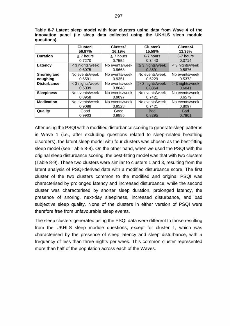
297
Table 8-7 Latent sleep model with four clusters using data from Wave 4 of the innovation panel (i.e sleep data collected using the UKHLS sleep module questions).
Cluster1 56.87%
Cluster2 16.19%
Cluster3 15.58%
Cluster4 11.36%
Duration ≥ 7 hours 0.7270
≥ 7 hours 0.7554
6-7 hours 0.3443
6-7 hours 0.3714
Latency < 3 nights/week 0.6075
No events/week 0.9668
≥ 3 nights/week 0.8591
< 3 nights/week 0.5876
Snoring and coughing
No events/week 0.6591
No events/week 0.9351
No events/week 0.5229
No events/week 0.5373
Disturbance < 3 nights/week 0.6039
No events/week 0.8048
≥ 3 nights/week 0.8864
≥ 3 nights/week 0.6041
Sleepiness No events/week 0.8958
No events/week 0.9097
No events/week 0.7421
No events/week 0.6579
Medication No events/week 0.9088
No events/week 0.9528
No events/week 0.7421
No events/week 0.8097
Quality Good 0.9903
Good 0.9885
Bad 0.8295
Bad 0.7801
After using the PSQI with a modified disturbance scoring to generate sleep patterns
in Wave 1 (i.e., after excluding questions related to sleep-related breathing
disorders), the latent sleep model with four clusters was chosen as the best-fitting
sleep model (see Table 8-8). On the other hand, when we used the PSQI with the
original sleep disturbance scoring, the best-fitting model was that with two clusters
(Table 8-9). These two clusters were similar to clusters 1 and 3, resulting from the
latent analysis of PSQI-derived data with a modified disturbance score. The first
cluster of the two clusters common to the modified and original PSQI was
characterised by prolonged latency and increased disturbance, while the second
cluster was characterised by shorter sleep duration, prolonged latency, the
presence of snoring, next-day sleepiness, increased disturbance, and bad
subjective sleep quality. None of the clusters in either version of PSQI were
therefore free from unfavourable sleep events.
The sleep clusters generated using the PSQI data were different to those resulting
from the UKHLS sleep module questions, except for cluster 1, which was
characterised by the presence of sleep latency and sleep disturbance, with a
frequency of less than three nights per week. This common cluster represented
more than half of the population across each of the Waves.

298
Table 8-8 Latent sleep model with four clusters using data from Wave 1 of the innovation panel (i.e. sleep data generated using the PSQI with modified disturbance component scores).
Cluster 1 54.54 %
Cluster2 37.46 %
Cluster3 62.10 %
Cluster4 17.90 %
Duration ≥ 7 hours 0.8553
≥ 7 hours 0.4631
6-7 hours 0.3220
≥ 7 hours 0.4986
Latency <3 nights/week 0.5213
<3 nights/week 0.7175
≥ 3 nights/week 0.8475
< 3 nights/week 0.6661
Snoring and breathing
No events/week 0.7430
No events/week 0.4917
<3 nights/week 0.5289
<3 nights/week 0.6975
Disturbance <3 nights/week 0.8978
<3 nights/week 0.8568
<3 nights/week 0.7432
≥ 3 nights/week 0.9192
Sleepiness and enthusiasm
No events/week 0.6462
<3 nights/week 0.7249
<3 nights/week 0.7137
<3 nights/week 0.6611
Medication No events/week 0.8920
No events/week 0.7683
No events/week 0.5937
≥ 3 nights/week 0.6371
Quality Good 0.9997
Good 0.6512
Bad 1.9787
Bad 0.8165
Table 8-9 Latent sleep model with four clusters using data from Wave 1 of the innovation panel (i.e. sleep data generated using the PSQI with original disturbance component scores).
Cluster 1 68.58%
Cluster 2 31.42%
Duration ≥ 7 hours 0.8045
6-7 hours 0.4026
Latency < 3 nights/week 0.5396
< 3 nights/week 0.6505
Snoring and coughing No events/week 0.7052
< 3 nights/week 0.4986
Disturbance < 3 nights/week 0.8819
< 3 nights/week 0.7774
Sleepiness No events/week 0.5729
< 3 nights/week 0.7341
Medication No events/week 0.8821
No events/week 0.6713
Quality Good 0.9963
Bad 0.6485
8.1.2.5 Discussion
In this study, the UKHLS sleep module was examined as a shorter version of the
PSQI, in order to enhance our understanding of sleep behaviours when generating
latent sleep patterns from data in the UKHLS, and how these might be applied to
pregnant participants in the UKHLS and Scott/Ciantar study. The relevance of
examining the PSQI in this was stemmed from its widespread use as perhaps the
most used sleep quality questionnaire, but which has proven to be unwieldy for use
in large population surveys due to the presence of several items with a long, poorly

299
justified and poorly conceptualised score algorithm. Unlike the PSQI, no scoring
system had been developed for the UKHLS sleep module questions, and this is
what led to studying this using LCA.
The internal consistency of the UKHLS sleep module questions was also examined
and found to be excellent; in contrast to the PSQI, which showed only moderate
internal consistency. The PSQI was reported by other researches to have an
internal consistency ranging from anywhere between 0.5 to 0.8 (Carpenter and
Andrykowski, 2016, Beck et al., 2004, Carpenter and Andrykowski, 1998). With a
higher internal consistency evident in the UKHLS sleep module questions, this
might reflect that its questions were better correlated and perhaps better on
measuring just one construct/characteristic at a time – suggesting that the UKHLS
sleep module questions offered a stronger basis with which to detect sleep patterns
once each of these constructs/characteristics were considered.
In this sub-study the correlation between each of the PSQI items and their
respective components were examined to verify if the UKHLS sleep module
questions were similar to those in the PSQI. The high correlations obtained indicate
the strength of associations between variables from each of these ‘questionnaires,
meaning that as the level of the first variable changes, the second will change
accordingly and, as a result, one of these variables can be substituted for the other
(notwithstanding the linguistic validity of the substituted item to represent the
relevant component in the other).
In the following section the linguistic validity of the UKHLS sleep module questions
will be discussed with regard to their representation of the relevant PSQI
components and their subsequent diagnostic value. The question, “How many
hours of actual sleep did you usually get at night during the last month?” from the
UKHLS sleep module is identical to question 4 in the PSQI, which aims to measure
subjective sleep length. Yet there were other questions in the PSQI for calculating
actual sleeping time. Actual sleeping time differs from the time spent in bed, which
many participants appeared to have usually recorded instead. Time spent in bed
included the actual time spent in bed, time needed to fall asleep (latency), and time
wasted in disturbed sleep (Olds et al., 2010). Although the UKHLS sleep module
questions do not measure the actual time spent sleeping, it has questions to
estimate the frequency of sleep latency and disturbance, which facilitate greater
understanding of the sleep patterns involved. That said, the lack of accuracy in the
measurement of actual sleeping hours appeared to have had an effect in the form
of measurement error when generating the latent sleep clusters and examining
their stability over time. Sleep duration had a low mean probability in the allocated

300
cluster (i.e., the certainty that the mean length of sleep duration of participants
belonging to a certain cluster was within that reported category). In addition, the
measurement error of sleep duration might be reflected in the instability of a sleep
duration pattern within clusters over Waves. Even so, the stability was a matter of
one to two hours, which was the difference between adjacent categories.
The question to determine if participants “cannot go to sleep within 30 min” is
identical to question 5 from the PSQI, which identifies the frequency of sleep
latency and is used to calculate the latency component after adding the score of
the question concerning “the length of sleep latency in minutes”. Delayed Phase
Circadian Rhythms Disorder patients differed from primary insomnia patients by
their recurrent or chronic sleep difficulties in sociable acceptable time. Delayed
Phase Circadian Rhythms Disorder patients developed sleep latency whenever
they were requested to sleep in time that mismatch their endogenous regulatory
cycle (Barion and Zee, 2007). This difference between the two conditions may be
difficult to spot thorough the UKHLS sleep module or PSQI questionnaires. People
who suffer from jet lag disorder have a misalignment between their endogenous
clock and their new environmental exogenous clock as a result of travelling. This
misalignment causes them to suffer from sleep latency (Bjorvatn and Pallesen,
2008). However, this cause of latency cannot be diagnosed using the two
questionnaires. The PSQI scoring for the latency component seems to
overestimate the severity of latency (sensitive), as the cluster with no abnormal
latency pattern was absent among the latent sleep clusters.
The question concerning sleep disturbance, by which the participant “wake[s] up
in the middle of the night or early in the morning,” is identical to Q5b in the PSQI,
which seeks, in addition to other questions, to define sleep disturbance.
Unfortunately, this question joins two different aspects of sleep disorders: early
waking and interrupted sleep. The early waking after uninterrupted sleep is a
symptom of Advanced Phase Disorder that is one of a circadian rhythm disorders
( Bjorvatn and Pallesen, 2008, Barion and Zee, 2007). Whereas early waking after
disturbed sleep may reflect primary insomnia (American Psychiatric Association,
2000). By contrast, disturbed sleep without early waking is seen in breath sleep
disorders and neurological sleep disorders patients (Kryger et al., 2011, American
Psychiatric Association, 2000). Similar to the latency score, the PSQI scoring for
the disturbance component seems to overestimate the severity of the disturbance
(sensitive), given that the cluster with a normal disturbance pattern was absent
among the latent sleep clusters.

301
The question concerning those participants who “cough or snore loudly” is identical
to Q5c in the PSQI, which, in addition to the question concerning the “presence of
breathing difficulty,” seeks to discover sleep disturbances secondary to Obstructive
Sleep Apnoea (OSA). Although not included in the PSQI score, the PSQI had
several questions evaluating the bed-partner’s attitude in regards their partner’s
snoring, as an individual may not be aware of his or her sleeping behaviour.
Snoring may be a symptom of OSA, which is occasionally linked with serious
diseases like heart and lung diseases (Kryger et al., 2011, American Psychiatric
Association, 2000). Snorers usually distinguished from the OSA patients by the
absence of interrupted sleep and daytime sleepiness (American Psychiatric
Association, 2000). Coughing is a symptom of respiratory or cardiovascular
diseases in addition to OSA, so including it in the question might decrease the
specificity to those with OSA (i.e., a false positive would result).
The question “During the past month how often have you had trouble staying
awake while driving, eating meals, or engaging in social activity?” is identical to Q8
from the PSQI, which is designed, in addition to the question concerning “the level
of enthusiasm,” to evaluate daytime dysfunction. Daytime sleepiness may be a
symptom of either fragmented nocturnal sleep or narcolepsy. Fragmented
nocturnal sleep is seen in primary insomnia and OSA patients (American
Psychiatric Association, 2000). Narcolepsy patients have prolonged and
undisturbed nocturnal sleep, while they have day time that is unexpected and
accompanied with hallucinations and catalepsy or muscle paralysis (American
Psychiatric Association, 2000). The day time sleep in narcolepsy is refreshing and
differentiates narcolepsy from other reasons of daytime sleepiness. However,
refreshing day sleepiness of narcolepsy should not be mistaken with normal daily
naps (American Psychiatric Association, 2000). Falling asleep during daily
activities indicates an advanced state of sleep deprivation or the presence of a
sleep disorder, thus falling asleep during activities might be used to differentiate
between those with and those without a severe form of sleep disturbance.
The question “During the last month how often have you taken medicine
(prescribed or over the counter) to help you sleep?” is identical to Q6 from the
PSQI. A limited number of questionnaires cover sleep medication. Usage of sleep
medications decrease sleep latency and improve quality but decrease morning
alertness and may alter behaviour (Parrott and Hindmarch, 1980). Knowing about
the usage of sleep medication explains the severity of the associated unfavourable
sleep events and allows the researchers to adjust for the effect of sleep
medications on sleep quality. However, this question might mislead by including

302
an “over the counter” in the question, as participants might interpret herbs, such as
chamomile taken in tea, as medicine.
The question “During the past month how would you rate your sleep quality
overall?” is identical to Q6 in the PSQI, which aims to evaluate a person’s attitude
toward his or her sleep quality. Poor sleep quality is a complaint in patients with
OSA, neurological sleep disorders, primary insomnia (American Psychiatric
Association, 2000) and in night-shift workers. Night shift worker’s poor sleep quality
appears in the form of “shortened sleep, fatigue, decreased alertness” (Bjorvatn
and Pallesen, 2008).
As indicated from the foregoing discussion, the ability of the two questionnaires to
describe sleep patterns differed. The PSQI was more sensitive to detecting sleep
disturbance and latency than the UKHLS sleep module. The sensitivity of PSQI
might be reflected in the LCA by the absence of a sleep pattern without latency or
disturbance. Day sleepiness and usage of medication indicated severe sleep
abnormalities that, unlike the UKHLS sleep module, the PSQI was able to detect.
This might be due to its sensitivity in detecting sleep disturbance and latency; thus,
as the number of participants with sleep disturbance and latency increased, the
probability of detecting and describing those participants who suffered from day
sleepiness and who used medication increased as well. However, due to the small
sample size, there might not be enough participants who shared severe forms of
sleep abnormalities in all components, so no cluster that had all abnormal sleep
characteristics was identified. Unfortunately, neither the PSQI nor the UKHLS
sleep module were able to diagnose sleep disorders, as both lack diagnostics
questions that are required to differentiate between sleep disorders that share
similar characteristics. However, the UKHLS sleep module showed a greater range
of patterns and less sensitivity than the PSQI, which might be useful in surveys
that are interested in depicting the variations in sleep patterns, rather than in clinical
sittings that require a diagnosis of sleep disorders.
In considering how much the included items in the UKHLS sleep module represent
the corresponding components in the PSQI, we examined the correlation between
the included items and the relevant component. The PSQI items that were included
in the UKHLS sleep module had higher correlations with their relevant component
scores than the items that were not included in the UKHLS sleep module. In
addition to the correlation, the included items in the UKHLS sleep module should
be comprehensive and serve the lingual and diagnostic purposes of the
components they will substitute.

303
The correlation value between the “frequency of the latency” question and the
latency component was very close to the correlation between the “minutes of sleep
latency” question and the latency component score. However, the former question
was more comprehensive, as it covered both the presence of prolonged latency (>
30 min.) and the frequency of latency. The correlation between the frequency of
mid-night or early-morning disturbances and the disturbance component was very
close to the correlation between the frequency of the disturbance secondary to
using the bathroom or pain. However, the frequency of mid-night or early-morning
disturbances was more representative and comprehensive of the disturbance
component than disturbance secondary to bathroom usage or pain, as the latter
appears in special occasions, such as pregnancy or old age. Including these two
questions in the UKHLS sleep module to cover latency and disturbance
components rather than the other questions that had almost similar correlations
was a better choice, as those two questions had more comprehensive information
than the other questions in the same components.
The next-day sleepiness (level of alertness) item was related more to sleep than
next-day dysfunction or enthusiasm, as the latter might be secondary to many
causes, such as mood disorders or poor health. We generated a component
relating to breathing disorders, for which we used two questions that were part of
the disturbance component. These questions concerned disturbance due to
breathing difficulty and disturbance secondary to snoring. The snoring item had the
highest correlation among the two questions with the calculated component score.
In addition, it was more sensitive than the “breathing difficulty” item in screening
for sleep breathing disorders. The use of the two questions was a specific method
by which to identify those with sleeping disorders who could not be identified
through assessment for snoring alone.
Considering the result of the latent class analysis, we find that the cluster patterns
resulting from the PSQI and the UKHLS sleep module were different except for
one cluster, which included more than half of the participants. The PSQI was very
sensitive to the presence of disturbance and latency, and perhaps overestimated
their presence, as there is no cluster that has an absence of unwanted sleep
events. By examining the variability of the sample, the percentage of participants
who reported unfavourable sleep events with a frequency of more than 3 nights
per week was limited. As a result, it would be expected from the LCA based on the
UKHLS sleep module that the cluster that is characterised by restricted sleep
duration (< 5 hours), bad quality, and unfavourable sleep events with a frequency
≥ 3 night per week would not be observed, due to the expected small size of that
cluster.

304
In summary, the UKHLS sleep module provides an acceptable comprehensive
screening for sleep and can be used as a short version of the PSQI, especially in
large-scale surveys. However, the UKHLS sleep module cannot be used as a
diagnostic tool for causes of poor sleep, as it lacks many diagnostic questions
needed to differentiate between several sleep disorders.
8.2 Systematic review and meta-analysis
8.2.1 Aspects of quality assessment of results
The focus of these quality assessments was the analytical validity of the published
results and the absence/presence of any potential biases, rather than the overall
quality of the published articles. However, as most of the current published studies
were designed to assess the quality of published papers, we decided to generate
guidelines that focused on the quality of the results instead of the quality of the
publication. Thus, we designed the guidelines based on other published checklists,
although we included only aspects that might interfere with the internal and/or
external validity of the results.
8.2.1.1 Generating a bespoke biases assessment guideline
8.2.1.1.1 Searching for current quality assessment tool
During our quality assessment of resultant observational studies, we generated
bespoke guidelines. The aim of the guidelines was to ensure that we covered all
issues that might bias the final estimates, instead of focusing on the quality of the
published papers. To achieve this, Google Scholar and Medline searches were
undertaken to look for any observational study-quality assessment tool that was
published before the end of 2014 (i.e., the beginning of our doctoral studies)7. In
the beginning, 32 tools were found, but 20 were excluded for not being validated.
Seven also were excluded, as they were designed for specific types of studies
other than medical observational studies (e.g., RCT). In the end, five were chosen:
‘Quality of reporting of observational longitudinal research checklist’ (Tooth et al.,
2005), ‘EPHPP statement’ (Thomas et al., 2004), ‘STROBE statement’ (Von Elm
et al., 2014), ‘Scottish Intercollegiate Guidelines Network (SIGN) checklists’ (SIGN,
2012) and ‘MOOSE statement’ (Stroup et al., 2000; Figure 8-3)
7 Please note that this search was not a typical systematic search as the aim was not to
generate a validated assessment tool instead the aim was to generate a simple useful guideline that will help in assessing the biases in the published results (instead of the quality of published papers) to use in this thesis.

305
Figure 8-3. Flow chart showing the number of included assessment tools
8.2.1.1.2 Application of the bespoke guideline in the assessment of biases
The 34 sleep and pregnancy studies found through a systematic search were all
included in the review, but not all regression models were included in the meta-
analysis, as each extracted regression model was evaluated carefully for the
possibility of adjustment bias before being considered for inclusion in the final
adjusted meta-analysis (Figure 8-4). Although all the resultant sleep and
pregnancy-outcome studies were included in the review, the results of the review
were determined after considering limitations and biases inherited from primary
studies. These limitations and biases were highlighted based on the bespoke
guidelines generated from the five quality-assessment checklists. The six aspects
we focused on were:
1) measurement bias;
2) confounding bias;
3) selection bias and generalizability of results;
4) multiple testing and type I errors;
5) sample size and type II errors; and
6) quality of results.
Finally, the results of the review were assessed for publication bias after
examining the quality of the included sleep and pregnancy outcomes’ primary
studies. A summary of the bespoke guidelines is presented in (Table 8-10)

306
8.2.1.2 Illustration of the bespoke bias assessment guideline
The bespoke bias-assessment guidelines covered six aspects of biases and
considered publication bias. The list of guidelines could be found in Table 8-10,
and in the following section, an illustration is provided on the aspects that were
considered during quality assessments.
Each outcome and/or exposure of interest was evaluated to see if it was the main
outcome or exposure of the assessed study. The power of the analysis and the
strategy of the study design depended on the rate of the main outcome and/or
exposure of the study ( Faul et al., 2009, Demidenko, 2006). If the outcome or
exposure was the main one, the study design was assessed for its type, as
randomized controlled trial (RCT) studies were the most favorable, followed by
cohort studies, case control studies, and cross-sectional studies. However, an RCT
can be difficult to perform due to ethical reasons, especially during pregnancy
(Khan et al., 1999). For that reason, it might be expected that there would be limited
numbers of RCT studies in regard to pregnancy outcomes. However, if the
outcome or exposure of interest were a secondary outcome or exposure that was
published due to its statistical significance (i.e., the outcome or exposure was not
considered when developing the study design and choosing the sample size), the
result was examined for the following: presence of selection bias or unadjusted
confounders; prevalence of the exposure and the outcome (rare events); presence
of type II errors (the power of the test); and the correction of the p-value for multiple
testing (type I error). Selection bias may have been a factor in choosing the study
population based on a characteristic of interest—for instance, high pregnancy BMI.
High pregnancy BMI is a mediator for early trimester sleep breathing disorders
(SBD), and adjusting for high BMI or excluding women with high BMI from the
analysis might bias the estimate. In contrast, late pregnancy SBD can be
precipitated by high BMI, and not adjusting for high BMI can lead to confounding
bias. In the case of rare events such as stillbirth, the study should be designed to
ensure a sufficient number of events to detect the association with sufficient
power—for example, by using a case control study design or by increasing the
length of the study period in the prospective longitudinal study. Not considering the
limited number of positive events in the design or the analysis can bias the
estimate, cause a wide confidence interval regardless of the sample size, and
increase the possibility of type II errors (Abeysena et al., 2009). Calculating the
sample size is very important for providing sufficient power to reject the null
hypothesis (Freiman et al., 1978) or to reduce type II errors. In the case of multiple
testing, due to the presence of more than one exposure and/or outcome,

307
consideration should be given to the alpha level, to reduce the chance of type I
errors (Cronbach, 1951, Bonferroni, 1936).
Inclusion and exclusion characteristics of the included participants were evaluated,
as restricting a study to one group can affect the generalisability of the result; for
instance, restricting the sample to snoring women could prevent generalising the
results to non-snoring women (Bossuyt et al., 2003).
The measurement tool used was examined for the possibility of measurement error
and the feasibility and timing of the measurement (i.e., the gestational age when
the measurement was taken). Objective measurements (such as
polysomnography (PSG)) may have less measurement error than subjective
measurements (such as sleep questionnaires), when considering sleep quantity or
the presence of SBD. On the other hand, subjective measurements are more
comprehensive and informative when measuring other sleep characteristics, such
as usage of sleep medication, lack of day refreshment, and sleep satisfaction.
However, accuracy and usage of subjective measurements can vary as well—for
instance, sleep diaries. Unlike questionnaires, sleep diaries can measure daily
fluctuations in sleep characteristics. Nevertheless, sleep questionnaires are easier
to analyze than sleep diaries, as the responses in the questionnaires are linked
with numbers that can be utilised in analysis.
With regard to feasibility of the measurement tool, PSG—which is considered
superior to other measurements of sleep duration—is difficult to apply over a long
period of time. Because of that, it could be difficult to find many prospective
longitudinal studies using PSG, especially when recurrent measurements of sleep
were taken. In addition, a PSG device can be uncomfortable to wear during sleep,
which might lead to shortened and fragmented sleep, especially in heavily pregnant
women who already find it difficult to sleep with an enlarged uterus. It was important
to consider the timing of measurements of sleep characteristics. Variables that
precipitate unfavorable sleep events in the late trimester can work as mediators for
unfavorable sleep events developed in the early trimester, such as high pregnancy
BMI and gestational diabetes. In addition, considering the variability of sleep during
pregnancy, it could be recommended to measure sleep more than once during
pregnancy, depending on the study design and duration. However, that might not
be feasible or easy to achieve, especially for a large population sample with
objective sleep measurements or in high-risk groups whose study compliance
might be a concern.
The definitions of sleep characteristics used, pregnancy outcomes, and included
study covariates were considered when comparing the results of studies. Several

308
studies used different cut-off points to define normal and abnormal sleep events.
For instance, a sleep duration longer than 9 hours per night was considered
abnormally long in some papers, and a duration longer than 8 hours was abnormal
in others. Similarly, pregnancy outcomes such macrosomia and Apgar scores were
defined using different reference points. In some papers, different variables were
considered to be similar; for instance, low birth weight and small for gestational
age as references to low birth weight are equally applicable for term and preterm
babies, while small for gestational age, premature, and term babies had different
reference weights. In addition, it was noticed that two outcomes with different
mechanisms were combined under one title—for example, preeclampsia and
pregnancy-induced hypertension. With regard to covariates, the single most
important factor in the definition was the timing—for instance, gestational age and
late pregnancy events. Gestational age when sleep was measured could be a
possible competing exposure, while gestational age when the outcome was
measured might be a possible mediator, depending on the study hypothesis and
design.
Studies were evaluated for the presence of a confounding bias. Confounders can
be adjusted during the study design or the analysis. Adjustment can be achieved
by restricting the study to a certain population, stratifying the study population into
sub-groups based on a character of interest, or by using multivariable regression
analysis. Study design can affect the amount of confounders present.
Observational studies—either cross sectional studies or longitudinal studies—may
have many unadjusted confounders in the study design, and careful adjustment is
required. Randomized controlled trials adjust for confounders in the design by
randomly assigning individuals to groups; however, unconsidered confounders
could affect the subsequent study estimate (for instance, participants’ height and
BMI; (Attia, 2005); for instance, limiting stratification of the data based on obesity
might limit the generalisability of the results to women of normal weight. In addition,
stratifying the sample could affect the power and the level confidence in the
estimate.
Adjustments of the regression models were evaluated with regard to the choice of
the adjusted confounders and the level of adjustment. Adjustment can be classified
as suitable, under-adjusted, unadjusted, and over-adjusted. Suitable adjustment
was defined as including the minimum acceptable number of confounders;
however, it might be difficult to cover all confounders, due to several limitations
(e.g., a limited number of participants or unavailable measurements in the data
registry). The regression models in the majority of the studies, especially cross-
sectional studies or studies without a control group, were considered under-

309
adjusted. Under-adjusted models were those that did not have all the minimum
acceptable confounders. Unadjusted or under-adjusted models might have a
confounding bias that overestimates or underestimates the association between
the exposure and the outcome of interest (Psaty et al., 1999). In over-adjusted
models (which include variables that are not confounders, such as competing
exposures or mediators), the unnecessary adjustment of variables might bias the
estimate when the model contains mediators (intermediate variables between the
exposure and the outcome that mediate the effect of the exposure on the outcome;
(Schisterman et al., 2009). However, including competing exposures (variables
that affect the outcome but are not related to the main exposure of interest), should
not bias the estimate but might narrow the CI level of the estimate and improve
precision (Textor and Li´skiewicz, 2017). The number of adjusted confounders
should be in proportion to the sample size, as including too many confounders
might affect the stability of the regression models and lead into inaccurate
estimation (Vittinghoff and McCulloch, 2006, Peduzzi, 1995). Finally, data were
evaluated for quality, ability to answer the research question, and presence and
treatment of missing data

310
Figure 8-4. Flow chart that illustrates the guidelines used in assessing the regression models before including them in the meta-analysis
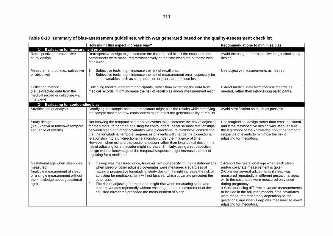
311
Table 8-10 summary of bias-assessment guidelines, which was generated based on the quality-assessment checklist
How might this aspect increase bias? Recommendations to minimize bias
1- Evaluating for measurement error
Retrospective or prospective study design
Retrospective design might increase the risk of recall bias if the exposure and confounders were measured retrospectively at the time when the outcome was measured.
Avoid the usage of retrospective longitudinal study design.
Measurement tool (i.e., subjective or objective)
1. Subjective tools might increase the risk of recall bias. 2. Subjective tools might increase the risk of measurement error, especially for
some variables such as sleep duration or post-partum blood loss.
Use objective measurements as needed.
Collection method (i.e., extracting data from the medical record or collecting via interview)
Collecting medical data from participants, rather than extracting the data from medical records, might increase the risk of recall bias and/or measurement error.
Extract medical data from medical records as needed, rather than interviewing participants.
2- Evaluating for confounding bias
Stratification of analysis Stratifying the sample based on mediators might bias the results while stratifying the sample based on how confounders might affect the generalizability of results.
Avoid stratification as much as possible.
Study design ( i.e., known or unknown temporal sequence of events)
Not knowing the temporal sequence of events might increase the risk of adjusting for mediators, rather than adjusting for confounders, because most relationships between sleep and other covariates were bidirectional relationships, considering that the longitudinal temporal sequences of events will change the bidirectional relationship into a unidirectional relationship under the influence of time. However, when using cross-sectional design rather than longitudinal design, the risk of adjusting for a mediator might increase. Similarly, using a retrospective design without knowledge of the temporal sequence might increase the risk of adjusting for a mediator.
Use longitudinal design rather than cross-sectional, and if the retrospective design was used, ensure the legitimacy of the knowledge about the temporal sequence of events to minimize the risk of adjusting for mediators.
Gestational age when sleep was measured (multiple measurement of sleep or a single measurement without the knowledge about gestational age)
1. If sleep was measured once, however, without specifying the gestational age when sleep or other adjusted covariates were measured (regardless of having a prospective longitudinal study design), it might increase the risk of adjusting for mediators, as it will not be clear which covariate preceded the other one.
2. The risk of adjusting for mediators might rise when measuring sleep and other covariates repeatedly without ensuring that the measurement of the adjusted covariates preceded the measurement of sleep.
1-Report the gestational age when each sleep and/or covariate measurement is taken. 2-Consider several adjustments if sleep was measured repeatedly in different gestational ages while the covariates were measured only once during pregnancy. 3-Consider using different covariate measurements to include in the adjusted models if the covariates were measured repeatedly depending on the gestational age when sleep was measured to avoid adjusting for mediators.

312
How might this aspect increase bias? Recommendations to minimize bias
Multiple testing and Type I errors
A questionnaire or a bespoke question
If a questionnaire was used rather than a single question. However, only one sleep characteristic was considered when presenting the result, which might raise the possibility of Type I errors or, in the final stage of the review, a publication bias.
Avoid reporting only significant results while neglecting insignificant results.
multiple outcomes or exposures If the authors did not adjust for the α level of multiple testing and presented their results using p-value (especially with a wide CI), this might raise the possibility of Type I errors.
1- Adjust the α level for multiple testing. 2- Avoid presenting the results based on p-value and neglecting the precision of the results.
3- Sample size and Type II errors
Sample size and power calculation
Not including a priori sample-size estimation or post hoc power calculation might increase the chances for type II errors.
A priori sample size estimation or post hoc power calculation should be included to estimate the magnitude of type II errors.
Stratification
Stratification might reduce the power of the test and increase the chances for type II errors.
Carefully consider stratification to avoid affecting the power of the analysis.
4- Selection bias and generalizability of results
Inclusion and exclusion criteria Excluding participants due to a characteristic that might be defined as a confounder (e.g., GDM, ethnicity) might interfere with the generalisability of results.
Carefully consider exclusion criteria.
Stratification of the sample Stratification of the results based on covariates that are thought to be confounders (e.g., BMI) might interfere with generalizability of results.
Avoid stratification by running multivariable analysis as needed.
Study settings Number: Including only one clinical setting might cause selection bias and affect the generalizability of results. Type: Running the study in a specific clinical setting, such as a high-risk antenatal care clinic, might affect the generalizability of results, as well as cause selection bias.
5- Quality of result
Missing data Missing data might cause a loss of information and bias the estimate (especially if the missing data were not missing randomly), as well as decrease the power of the analysis and elevate the chances for type II errors if they were excluded, rather than imputed.
Carefully evaluate missing data for missing at random assumption and apply multiple imputation as needed.
6- Publication bias
Signs of publication bias: Carefully consider publication bias.

313
How might this aspect increase bias? Recommendations to minimize bias
1- Most results were significant. 2- Most of the study used a small sample size with underpowered
regression models. 3- Most of the reported OR were large, and the CI lacked precision. 4- Multiple flaws in the design of the published primary studies 5- Severe heterogeneity between the results or in the other extreme
repeated studies with similar results
8.2.2 Descriptive results of the systematic review
Figure 8-5 Line graph showing the number of articles in the searches conducted per year of publication.
0
1
2
3
4
5
6
7
8
2000 2002 2004 2006 2008 2010 2012 2014 2016 2018
Nu
mb
er
of
refr
en
ces
Year of publication

314
8.3 Sleep Patterns in the United Kingdom Population: a latent
class analysis of the UKHLS
8.3.1 Coding sociodemographic features and health indicators
Table 8-11 Sociodemographic features of interest together with their original and new categorisations.
Variable Original categorization New categorization
Gender
Gender Male Male Female Female
Age
Q: Age at the time of interview
10-19 years old ≤19 years 20-29 years old
20-39years 30-39 years old 40-49 years old
40-59 years 50-59 years old 60-69 years old
≥ 60 years 70 years or older
Education
Q: Current status of highest educational or vocational qualification
Degree A level and above
Other higher A level and others GCSE and others
GCSE level and others
Other qualification No qualification
Occupation
Q: Current employment situation
Self employed
Employed Unpaid family business Doing something else Paid employment(ft/pt) Unemployed
Unemployed Family care or home On maternity leave
Sick or disabled Sick or disabled Government training scheme
Training or education
Full-time student On apprenticeship Retired Retired
Household structure
Q: This was a derived variable generated from several questions in regards to age , presence of couple and number of adult and children in the household
1 male, aged 65+, no children
Single without children
1 female, age 60+, no children 1 adult under pensionable age, no children 2 adults, not a couple, both under pensionable age, no children 2 adults, not a couple, one or more over pensionable age, no children 3 or more adults, no children, excl. any couples 1 adult, 1 child
Single with children
1 adult, 2 or more children 2 adults, not a couple, 1 or more children
Couple both under pensionable age, no children Couple without children
Couple 1 or more over pensionable age, no children
3 or more adults, 1 or more children excl. any couples Couple with 1 child
Couple with children
Couple with 2 children Couple with 3 or more children 3 or more adults, no children, incl. at least one couple 3 or more adults, 1-2 children, incl. at least one couple

315
Table 8-12 SF12v questionnaire used in the UKHLS. The questions and responses were a modified combination of both the SF12v1 and SF12v2.
Subdomain Question Response
General health
1-In general, would you say your health is... 1-Excellent 2-Very good 3-Good 4-Fair 5-Poor
Physical health
2-The following questions are about activities you might do during a typical day. a- Does your health now limit you in these activities? If so, how much? Moderate activities, such as moving a table, pushing a vacuum cleaner, bowling or playing golf b- Does your health now limit you in these activities? If so, how much?) Climbing several flights of stairs
1-Yes, limited a lot 2-Yes, limited a little 3-No, not limited at all
Physical health (role functioning)
3a--During the past 4 weeks, how much of the time have you had any of the following problems with your work or other regular daily activities as a result of your physical health? Accomplished less than you would like 3b-During the past 4 weeks, how much of the time have you had any of the following problems with your work or other regular daily activities as a result of your physical health?) Were limited in the kind of work or other activities
1-All of the time 2-Most of the time 3-Some of the time 4-A little of the time 5-None of the time
Emotional (role functioning)
4a-During the past 4 weeks, how much of the time have you had any of the following problems with your work or other regular daily activities as a result of any emotional problems (such as feeling depressed or anxious)? Accomplished less than you would like 4b-(During the past 4 weeks, how much of the time have you had any of the following problems with your work or other regular daily activities as a result of any emotional problems (such as feeling depressed or anxious)?) Did work or other activities less carefully than usual
1-All of the time 2-Most of the time 3-Some of the time 4-A little of the time 5-None of the time
Bodily pain 5-During the past 4 weeks, how much did pain interfere with your normal work (including both work outside the home and housework)?
1-Not at all 2-A little bit 3-Moderately 4-Quite a bit 5-Extremely
6-These questions are about how you feel and how things have been with you during the past 4 weeks. For each question, please give the one answer that comes closest to the way you have been feeling.
1-All of the time 2-Most of the time 3-Some of the time 4-A little of the time 5-None of the time Mental
health
a- Have you felt calm and peaceful? b- Did you have a lot of energy?
Mental health
c- Have you felt downhearted and depressed?
Social health
d- How much of the time has your physical health or emotional problems interfered with your social activities (like visiting friends or relatives)?

316
8.3.2 Choosing best fit model
Table 8-13 the iteration criteria observed for latent models generated using LCA to UKHLS sleep module data.
The Bold text indicates the chosen iteration criteria values
Stability study Complete population study
Wave 1 Wave 4
Goodness of fit Entropy measurements
Goodness of fit Entropy measurements
Goodness of fit Entropy measurements
Model BIC AIC Number of parameters
R2 CE BIC AIC Number of parameters
R2 CE BIC AIC Number of parameters
R2 CE
Model1 213405 213295 14 1.00 0.00 202112 202001 14 1.00 0.00 575342 575220 14 1.00 0.00
Model2 198887 198713 22 0.79 0.06 186782 186608 22 0.78 0.04 331168 330970 22 0.78 0.06
Model3 197069 196833 30 0.69 0.11 185479 185242 30 0.67 0.13 312114 311853 30 0.71 0.11
Model4 196340 196040 38 0.67 0.15 184506 184206 38 0.71 0.13 309722 309391 38 0.68 0.15
Model5 196115 195753 46 0.68 0.17 184099 183753 46 0.68 0.17 308702 308301 46 0.69 0.15
Model6 195502 195328 54 0.68 0.14 183819 183364 54 0.74 0.15 307816 307620 54 0.73 0.14
Model7 195626 195430 62 0.66 0.18 183861 183371 62 0.72 0.17 307864 307696 62 0.68 0.17
Model8 195753 195551 70 0.66 0.18 183672 183318 70 0.69 0.17 307745 307585 70 0.66 0.18
Model9 195429 195315 78 0.66 0.19 183515 183298 78 0.65 0.19 307574 307472 78 0.66 0.19
Model10 195481 195254 86 0.63 0.27 183534 183154 86 0.68 0.21 307489 307339 86 0.63 0.27

317
8.3.3 Choosing best fit model (binary coding of data)
Table 8-14 BIC values and the number of parameters observed for latent sleep models generated using exploratory latent class analyses using binary coding for each of the sleep variables.
Stability study (n=19,442)
Complete population study (n=45, 141)
Wave 1 Wave 4
Number of
parameters
BIC Number of parameter
s BIC
Number of parameters
BIC
1 Cluster 7 151509.3 7 139987.9 7 338323.2
2 Clusters 15 142591.1 15 130987.4 15 316944
3 Clusters 23 140624.4 23 129700.6 23 312662.9
4 Clusters 31 140497 31 129654.4 31 312294.9
5 Clusters 39 140499.5 39 129703.1 39 312082.5
6 Clusters 47 140543.9 47 129753.5 47 312128.5
7 Clusters 55 140541.2 55 129789.3 55 312143.8
8 Clusters 63 140611.4 63 129861.1 63 312178.9
9 Clusters 71 140671.4 71 129927.7 71 312234.4
10 Clusters 79 140734.2 79 130005.5 79 312348.6
The Bold text indicates the chosen BIC values after considering the number of parameters
8.3.4 Latent sleep pattern models (using binary coded of data)
Table 8-15 Wave 1 matched population (n=19,442) cluster patterns using binary variables.
Cluster 1 Cluster 2 Cluster 3 Cluster 4 Cluster 5
Duration ≥ 7 hours
0.252
≥ 7 hours
0.174
< 7 hours
0.7868
< 7 hours
0.715
≥ 7 hours
0.096
Latency Present
0.633 Absent 0.169
Present 0.922
Present
0.697
Present
0.801
Snoring Absent
0.399
Absent
0.126
Present
0.649
Absent
0.210
Present
0.610
Disturbance Present
0.952
Absent
0.246
Present
0.995
Present
0.878
Present
0.927
Sleepiness Absent
0.108
Absent
0.072
Absent
0.345
Absent
0.260
Absent
0.215
Medication Absent
0.071
Absent
0.0812
Absent
0.367
Absent
0.129
Present
0.689
Quality Absent
0.012
Absent
0.001
Present
0.790
Present
0.889
Absent
0.099

318
Table 8-16 UKHLS Wave 4 matched population (n=19,442) sleep cluster patterns generated using binary variables.
Cluster 1 Cluster 2 Cluster 3 Cluster 4 Cluster 5
Duration ≥ 7 hours 0.200
≥ 7 hours
0.265
< 7 hours
0.863
≥ 7 hours
0.425
< 7 hours
0.789
Latency Absent 0.176
Present 0.664
Present 0.860
Present
0.718
Absent
0.484
Snoring Absent
0.082
Absent
0.296
Absent 0.313
Absent
0.226
Absent 0.169
Disturbance Absent
0.303
Present
0.854
Present
0.980
Present
0.946
Present
0.698
Sleepiness Absent
0.035
Absent
0.162
Absent
0.206
Absent
0.008
Absent
0.217
Medication Absent
0.012
Absent
0.118
Absent
0.236
Absent
0.015
Present
0.011
Quality Absent
0.001
Absent
0.012
Present
0.885
Absent
0.027
Absent
0.381
Table 8-17 UKHLS Wave 1 and 4 (n=45,141) sleep cluster patterns generated using binary variables.
Cluster 1 Cluster 2 Cluster 3 Cluster 4 Cluster 5 Cluster 6
Duration ≥ 7 hours 0.264
≥ 7 hours
0.177
< 7 hours
0.807
≥ 7 hours
0.179
< 7 hours
0.865
≥ 7 hours 0.192
Latency Present 0.627
Absent 0.172
Present 0.932
Present
0.777
Present 0.626
Present 0.768
Snoring Absent
0.383
Absent
0.100
Present
0.544
Absent
0.059
Absent 0.181
Present
0.858
Disturbance Present
0.957
Absent
0.223
Present
0.999
Present
0.805
Present
0.844
Present
0.888
Sleepiness Absent
0.031
Absent
0.038
Absent
0.198
Absent
0.142
Absent
0.159
Absent
0.275
Medication Absent
0.071
Absent 0.056
Absent
0.330
Absent
0.113
Absent
0.120
Absent
0.388
Quality Absent
0.008
Absent 0.001
Present
0.822
Absent
0.154
Present
0.706
Absent
0.174

319
8.3.5 Algorithm of generated latent sleep patterns
Table 8-18 Latent sleep patterns coding algorithm generated using latent class analysis.
Q= quality, SL= sleepiness, M= medication, SN= snoring and/or coughing, D= disturbance, L= latency, SD= sleep duration, FO= frequency of observations, LSP= latent sleep pattern.
Q SL M SN D L SD FO LSP
1 0 1 1 2 1 2 8 3
1 0 1 1 2 1 3 2 3
1 0 1 1 2 2 0 12 3
1 0 1 1 2 2 1 6 3
1 0 1 1 2 2 2 1 3
1 0 1 2 0 0 0 8 1
1 0 1 2 0 0 1 2 1
1 0 1 2 0 0 2 1 1
1 0 1 2 0 1 0 1 1
1 0 1 2 0 1 1 2 1
1 0 1 2 0 2 0 1 1
1 0 1 2 1 0 0 18 1
1 0 1 2 1 0 1 3 1
1 0 1 2 1 1 0 36 1
1 0 1 2 1 1 1 7 1
1 0 1 2 1 1 2 2 1
1 0 1 2 1 2 0 5 1
1 0 1 2 1 2 1 1 1
1 0 1 2 2 0 0 15 1
1 0 1 2 2 0 1 1 1
1 0 1 2 2 1 0 15 1
1 0 1 2 2 1 1 5 3
1 0 1 2 2 2 0 16 3
1 0 1 2 2 2 1 14 3
1 0 1 2 2 2 2 4 3
1 0 2 0 0 0 0 166 2
1 0 2 0 0 0 1 22 2
1 0 2 0 0 0 2 5 2
1 0 2 0 0 0 3 2 2
1 0 2 0 0 1 0 28 1
1 0 2 0 0 1 1 3 1
1 0 2 0 0 2 0 6 1
1 0 2 0 1 0 0 82 1
1 0 2 0 1 0 1 14 1
1 0 2 0 1 0 2 3 1
1 0 2 0 1 1 0 121 1
1 0 2 0 1 1 1 17 1
1 0 2 0 1 1 2 2 4
1 0 2 0 1 1 3 2 4
1 0 2 0 1 2 0 19 1
1 0 2 0 1 2 1 6 1
1 0 2 0 2 0 0 67 1

320
Q SL M SN D L SD FO LSP
1 0 1 1 2 1 2 8 3
1 0 1 1 2 1 3 2 3
1 0 1 1 2 2 0 12 3
1 0 1 1 2 2 1 6 3
1 0 1 1 2 2 2 1 3
1 0 1 2 0 0 0 8 1
1 0 1 2 0 0 1 2 1
1 0 2 0 2 0 1 23 1
1 0 2 0 2 0 2 5 6
1 0 2 0 2 0 3 1 6
1 0 2 0 2 1 0 51 1
1 0 2 0 2 1 1 27 3
1 0 2 0 2 1 2 2 3
1 0 2 0 2 2 0 27 3
1 0 2 0 2 2 1 17 3
1 0 2 0 2 2 2 10 3
1 0 2 0 2 2 3 4 3
1 0 2 1 0 0 0 22 1
1 0 2 1 0 0 1 1 1
1 0 2 1 0 0 2 2 1
1 0 2 1 0 1 0 7 1
1 0 2 1 0 2 0 1 1
1 0 2 1 1 0 0 39 1
1 0 2 1 1 0 1 5 1
1 0 2 1 1 1 0 64 1
1 0 2 1 1 1 1 13 1
1 0 2 1 1 1 2 2 4
1 0 2 1 1 1 3 2 4
1 0 2 1 1 2 0 8 1
1 0 2 1 1 2 1 2 4
1 0 2 1 1 2 2 1 4
1 0 2 1 1 2 3 1 4
1 0 2 1 2 0 0 14 1
1 0 2 1 2 0 1 1 6
1 0 2 1 2 1 0 40 1
1 0 2 1 2 1 1 8 3
1 0 2 1 2 2 0 16 3
1 0 2 1 2 2 1 9 3
1 0 2 1 2 2 2 1 3
1 0 2 1 2 2 3 1 3
1 0 2 2 0 0 0 16 1
1 0 2 2 0 0 1 2 1
1 0 2 2 0 0 2 1 1
1 0 2 2 0 1 0 2 1
1 0 2 2 0 1 1 3 1
1 0 2 2 0 2 0 2 1
1 0 2 2 1 0 0 29 1
1 0 2 2 1 0 1 7 1
1 0 2 2 1 0 2 1 1
1 0 2 2 1 1 0 37 1
1 0 2 2 1 1 1 9 1

321
Q SL M SN D L SD FO LSP
1 0 1 1 2 1 2 8 3
1 0 1 1 2 1 3 2 3
1 0 1 1 2 2 0 12 3
1 0 1 1 2 2 1 6 3
1 0 1 1 2 2 2 1 3
1 0 1 2 0 0 0 8 1
1 0 1 2 0 0 1 2 1
1 0 2 2 1 1 2 2 4
1 0 2 2 1 2 0 3 1
1 0 2 2 1 2 1 3 4
1 0 2 2 2 0 0 30 1
1 0 2 2 2 0 1 7 6
1 0 2 2 2 0 3 1 6
1 0 2 2 2 1 0 39 3
1 0 2 2 2 1 1 21 3
1 0 2 2 2 1 2 2 3
1 0 2 2 2 1 3 1 3
1 0 2 2 2 2 0 32 3
1 0 2 2 2 2 1 16 3
1 0 2 2 2 2 2 6 3
1 0 2 2 2 2 3 1 3
1 1 0 0 0 0 0 182 2
1 1 0 0 0 0 1 59 2
1 1 0 0 0 0 2 12 2
1 1 0 0 0 0 3 4 2
1 1 0 0 0 1 0 69 1
1 1 0 0 0 1 1 19 1
1 1 0 0 0 1 2 1 4
1 1 0 0 0 1 3 1 4
1 1 0 0 0 2 0 11 1
1 1 0 0 0 2 1 5 4
1 1 0 0 0 2 2 1 4
1 1 0 0 0 2 3 1 4
1 1 0 0 1 0 0 165 1
1 1 0 0 1 0 1 46 1
1 1 0 0 1 0 2 13 1
1 1 0 0 1 1 0 299 1
1 1 0 0 1 1 1 85 1
1 1 0 0 1 1 2 10 4
1 1 0 0 1 1 3 5 4
1 1 0 0 1 2 0 53 1
1 1 0 0 1 2 1 9 4
1 1 0 0 1 2 2 4 4
1 1 0 0 1 2 3 1 4
1 1 0 0 2 0 0 60 1
1 1 0 0 2 0 1 39 1
1 1 0 0 2 0 2 9 6
1 1 0 0 2 0 3 1 6
1 1 0 0 2 1 0 85 1
1 1 0 0 2 1 1 40 1
1 1 0 0 2 1 2 5 6

322
Q SL M SN D L SD FO LSP
1 0 1 1 2 1 2 8 3
1 0 1 1 2 1 3 2 3
1 0 1 1 2 2 0 12 3
1 0 1 1 2 2 1 6 3
1 0 1 1 2 2 2 1 3
1 0 1 2 0 0 0 8 1
1 0 1 2 0 0 1 2 1
1 1 0 0 2 1 3 1 6
1 1 0 0 2 2 0 27 3
1 1 0 0 2 2 1 15 3
1 1 0 0 2 2 2 2 3
1 1 0 0 2 2 3 2 3
1 1 0 1 0 0 0 24 1
1 1 0 1 0 0 1 7 1
1 1 0 1 0 0 2 3 1
1 1 0 1 0 1 0 21 1
1 1 0 1 0 1 1 5 1
1 1 0 1 0 2 0 2 1
1 1 0 1 0 2 1 1 4
1 1 0 1 1 0 0 61 1
1 1 0 1 1 0 1 27 1
1 1 0 1 1 0 2 4 1
1 1 0 1 1 1 0 168 1
1 1 0 1 1 1 1 50 1
1 1 0 1 1 1 2 12 4
1 1 0 1 1 1 3 1 4
1 1 0 1 1 2 0 14 1
1 1 0 1 1 2 1 8 4
1 1 0 1 1 2 2 1 4
1 1 0 1 2 0 0 32 1
1 1 0 1 2 0 1 9 6
1 1 0 1 2 0 2 3 6
1 1 0 1 2 1 0 56 1
1 1 0 1 2 1 1 36 3
1 1 0 1 2 1 2 2 3
1 1 0 1 2 1 3 1 6
1 1 0 1 2 2 0 21 3
1 1 0 1 2 2 1 10 3
1 1 0 1 2 2 2 3 3
1 1 0 2 0 0 0 18 1
1 1 0 2 0 0 1 5 1
1 1 0 2 0 0 3 2 4
1 1 0 2 0 1 0 8 1
1 1 0 2 0 1 1 6 1
1 1 0 2 0 2 1 1 4
1 1 0 2 0 2 2 1 4
1 1 0 2 1 0 0 19 1
1 1 0 2 1 0 1 4 1
1 1 0 2 1 0 2 2 1
1 1 0 2 1 1 0 39 1
1 1 0 2 1 1 1 19 1

323
Q SL M SN D L SD FO LSP
1 0 1 1 2 1 2 8 3
1 0 1 1 2 1 3 2 3
1 0 1 1 2 2 0 12 3
1 0 1 1 2 2 1 6 3
1 0 1 1 2 2 2 1 3
1 0 1 2 0 0 0 8 1
1 0 1 2 0 0 1 2 1
1 1 0 2 1 1 2 3 4
1 1 0 2 1 2 0 6 1
1 1 0 2 1 2 1 3 4
1 1 0 2 1 2 3 1 4
1 1 0 2 2 0 0 21 1
1 1 0 2 2 0 1 9 6
1 1 0 2 2 0 2 1 6
1 1 0 2 2 0 3 1 6
1 1 0 2 2 1 0 33 1
1 1 0 2 2 1 1 22 3
1 1 0 2 2 1 2 3 3
1 1 0 2 2 2 0 16 3
1 1 0 2 2 2 1 9 3
1 1 0 2 2 2 2 1 3
1 1 0 2 2 2 3 2 3
1 1 1 0 0 0 0 40 2
1 1 1 0 0 0 1 6 2
1 1 1 0 0 0 2 1 2
1 1 1 0 0 1 0 15 1
1 1 1 0 0 1 1 2 1
1 1 1 0 0 2 0 1 1
1 1 1 0 0 2 1 1 4
1 1 1 0 1 0 0 9 1
1 1 1 0 1 0 1 4 1
1 1 1 0 1 1 0 38 1
1 1 1 0 1 1 1 6 1
1 1 1 0 1 1 2 2 4
1 1 1 0 1 1 3 1 4
1 1 1 0 1 2 0 4 1
1 1 1 0 2 0 0 1 1
1 1 1 0 2 0 1 5 6
1 1 1 0 2 1 0 11 1
1 1 1 0 2 1 1 5 3
1 1 1 0 2 2 0 6 3
1 1 1 0 2 2 1 2 3
1 1 1 0 2 2 2 1 3
1 1 1 1 0 0 0 5 1
1 1 1 1 0 0 1 1 1
1 1 1 1 0 1 0 5 1
1 1 1 1 0 1 1 1 1
1 1 1 1 0 1 2 2 4
1 1 1 1 0 2 0 1 1
1 1 1 1 1 0 0 10 1
1 1 1 1 1 0 1 1 1

324
Q SL M SN D L SD FO LSP
1 0 1 1 2 1 2 8 3
1 0 1 1 2 1 3 2 3
1 0 1 1 2 2 0 12 3
1 0 1 1 2 2 1 6 3
1 0 1 1 2 2 2 1 3
1 0 1 2 0 0 0 8 1
1 0 1 2 0 0 1 2 1
1 1 1 1 1 0 3 1 4
1 1 1 1 1 1 0 37 1
1 1 1 1 1 1 1 20 1
1 1 1 1 1 1 2 6 4
1 1 1 1 1 1 3 1 4
1 1 1 1 1 2 0 3 1
1 1 1 1 2 0 0 1 1
1 1 1 1 2 0 1 1 6
1 1 1 1 2 1 0 20 1
1 1 1 1 2 1 1 4 3
1 1 1 1 2 1 2 1 3
1 1 1 1 2 1 3 1 6
1 1 1 1 2 2 0 6 3
1 1 1 1 2 2 1 5 3
1 1 1 2 0 0 1 1 1
1 1 1 2 0 1 0 1 1
1 1 1 2 1 0 0 4 1
1 1 1 2 1 0 2 1 1
1 1 1 2 1 1 0 13 1
1 1 1 2 1 1 1 6 1
1 1 1 2 1 2 0 2 1
1 1 1 2 1 2 1 3 4
1 1 1 2 1 2 2 1 4
1 1 1 2 2 0 0 1 1
1 1 1 2 2 0 1 3 6
1 1 1 2 2 1 0 6 3
1 1 1 2 2 1 1 5 3
1 1 1 2 2 1 2 1 3
1 1 1 2 2 1 3 1 3
1 1 1 2 2 2 0 7 3
1 1 1 2 2 2 1 4 3
1 1 1 2 2 2 2 1 3
1 1 2 0 0 0 0 13 2
1 1 2 0 0 0 1 4 2
1 1 2 0 0 1 0 4 1
1 1 2 0 1 0 0 12 1
1 1 2 0 1 0 1 2 1
1 1 2 0 1 0 2 1 4
1 1 2 0 1 1 0 19 1
1 1 2 0 1 1 1 5 1
1 1 2 0 1 1 3 1 4
1 1 2 0 1 2 0 3 1
1 1 2 0 1 2 1 3 4
1 1 2 0 2 0 0 4 1

325
Q SL M SN D L SD FO LSP
1 0 1 1 2 1 2 8 3
1 0 1 1 2 1 3 2 3
1 0 1 1 2 2 0 12 3
1 0 1 1 2 2 1 6 3
1 0 1 1 2 2 2 1 3
1 0 1 2 0 0 0 8 1
1 0 1 2 0 0 1 2 1
1 1 2 0 2 0 1 1 6
1 1 2 0 2 1 0 8 1
1 1 2 0 2 1 1 2 3
1 1 2 0 2 1 2 1 3
1 1 2 0 2 2 0 1 3
1 1 2 0 2 2 1 1 3
1 1 2 0 2 2 2 2 3
1 1 2 0 2 2 3 2 3
1 1 2 1 0 0 0 1 1
1 1 2 1 0 1 0 3 1
1 1 2 1 1 0 0 2 1
1 1 2 1 1 0 2 1 4
1 1 2 1 1 1 0 17 1
1 1 2 1 1 1 1 5 4
1 1 2 1 1 1 3 1 4
1 1 2 1 1 2 0 1 1
1 1 2 1 1 2 1 1 4
1 1 2 1 2 0 0 2 1
1 1 2 1 2 0 1 1 6
1 1 2 1 2 1 0 6 3
1 1 2 1 2 1 1 2 3
1 1 2 1 2 2 0 3 3
1 1 2 1 2 2 1 3 3
1 1 2 2 0 0 0 4 1
1 1 2 2 0 1 0 1 1
1 1 2 2 0 1 1 1 4
1 1 2 2 1 0 0 6 1
1 1 2 2 1 0 1 2 1
1 1 2 2 1 0 2 1 4
1 1 2 2 1 1 0 5 1
1 1 2 2 1 1 1 3 4
1 1 2 2 1 1 2 1 4
1 1 2 2 1 2 0 6 4
1 1 2 2 1 2 1 1 4
1 1 2 2 2 0 0 9 1
1 1 2 2 2 0 1 1 6
1 1 2 2 2 0 2 1 6
1 1 2 2 2 1 0 11 3
1 1 2 2 2 1 1 2 3
1 1 2 2 2 1 2 1 3
1 1 2 2 2 2 0 4 3
1 1 2 2 2 2 1 2 3
1 1 2 2 2 2 2 2 3
1 1 2 2 2 2 3 1 3

326
Q SL M SN D L SD FO LSP
1 0 1 1 2 1 2 8 3
1 0 1 1 2 1 3 2 3
1 0 1 1 2 2 0 12 3
1 0 1 1 2 2 1 6 3
1 0 1 1 2 2 2 1 3
1 0 1 2 0 0 0 8 1
1 0 1 2 0 0 1 2 1
1 2 0 0 0 0 0 10 2
1 2 0 0 0 0 1 3 2
1 2 0 0 0 0 2 4 4
1 2 0 0 0 1 1 1 4
1 2 0 0 0 2 0 1 4
1 2 0 0 0 2 1 1 4
1 2 0 0 1 0 0 5 1
1 2 0 0 1 0 1 1 1
1 2 0 0 1 0 2 1 4
1 2 0 0 1 1 0 4 1
1 2 0 0 1 1 1 1 4
1 2 0 0 1 1 2 1 4
1 2 0 0 1 2 0 1 4
1 2 0 0 1 2 1 1 4
1 2 0 0 2 0 0 4 1
1 2 0 0 2 0 1 1 6
1 2 0 0 2 0 3 1 6
1 2 0 0 2 1 0 6 1
1 2 0 0 2 1 1 1 6
1 2 0 0 2 2 0 4 3
1 2 0 0 2 2 1 3 3
1 2 0 0 2 2 3 1 3
1 2 0 1 0 0 0 2 1
1 2 0 1 0 0 1 2 1
1 2 0 1 0 1 1 1 4
1 2 0 1 1 0 0 3 1
1 2 0 1 1 1 0 4 1
1 2 0 1 2 0 0 2 1
1 2 0 1 2 0 1 1 6
1 2 0 1 2 1 0 1 1
1 2 0 1 2 1 1 1 3
1 2 0 1 2 1 2 1 6
1 2 0 1 2 2 0 3 3
1 2 0 2 0 0 0 2 1
1 2 0 2 0 1 0 2 1
1 2 0 2 0 2 0 1 4
1 2 0 2 1 0 1 1 1
1 2 0 2 1 0 2 1 4
1 2 0 2 1 1 0 4 1
1 2 0 2 1 2 0 1 4
1 2 0 2 1 2 1 1 4
1 2 0 2 1 2 2 1 4
1 2 0 2 2 0 0 3 1
1 2 0 2 2 0 2 3 6

327
Q SL M SN D L SD FO LSP
1 0 1 1 2 1 2 8 3
1 0 1 1 2 1 3 2 3
1 0 1 1 2 2 0 12 3
1 0 1 1 2 2 1 6 3
1 0 1 1 2 2 2 1 3
1 0 1 2 0 0 0 8 1
1 0 1 2 0 0 1 2 1
1 2 0 2 2 1 0 1 3
1 2 0 2 2 1 1 1 3
1 2 0 2 2 2 0 5 3
1 2 0 2 2 2 3 2 3
1 2 1 0 0 0 0 1 2
1 2 1 0 1 0 0 1 1
1 2 1 0 2 1 0 1 1
1 2 1 0 2 2 0 1 3
1 2 1 1 0 0 0 1 1
1 2 1 1 0 2 1 1 4
1 2 1 1 1 0 0 1 1
1 2 1 1 1 0 1 1 1
1 2 1 1 1 1 1 1 4
1 2 1 2 1 0 0 1 1
1 2 1 2 2 2 0 4 3
1 2 1 2 2 2 1 1 3
1 2 1 2 2 2 3 1 5
1 2 2 0 0 0 0 1 2
1 2 2 0 0 0 1 1 4
1 2 2 0 1 0 0 1 1
1 2 2 0 1 2 0 1 4
1 2 2 0 2 0 0 1 6
1 2 2 0 2 0 1 1 6
1 2 2 0 2 0 3 1 6
1 2 2 0 2 1 0 2 1
1 2 2 0 2 1 1 1 6
1 2 2 0 2 2 0 2 3
1 2 2 0 2 2 1 1 3
1 2 2 1 1 0 1 1 4
1 2 2 1 1 1 1 1 4
1 2 2 1 2 0 0 1 6
1 2 2 1 2 1 0 1 3
1 2 2 2 0 0 0 1 1
1 2 2 2 1 1 0 2 4
1 2 2 2 1 2 0 1 4
1 2 2 2 2 0 0 2 6
1 2 2 2 2 0 1 1 6
1 2 2 2 2 1 0 4 3
1 2 2 2 2 1 1 2 3
1 2 2 2 2 2 0 2 3
1 2 2 2 2 2 1 2 3
2 0 0 0 0 0 0 21 2
2 0 0 0 0 0 1 26 4
2 0 0 0 0 0 2 14 4

328
Q SL M SN D L SD FO LSP
1 0 1 1 2 1 2 8 3
1 0 1 1 2 1 3 2 3
1 0 1 1 2 2 0 12 3
1 0 1 1 2 2 1 6 3
1 0 1 1 2 2 2 1 3
1 0 1 2 0 0 0 8 1
1 0 1 2 0 0 1 2 1
2 0 0 0 0 0 3 12 4
2 0 0 0 0 1 0 18 4
2 0 0 0 0 1 1 20 4
2 0 0 0 0 1 2 3 4
2 0 0 0 0 2 0 24 4
2 0 0 0 0 2 1 18 4
2 0 0 0 0 2 2 8 4
2 0 0 0 0 2 3 9 4
2 0 0 0 1 0 0 28 4
2 0 0 0 1 0 1 16 4
2 0 0 0 1 0 2 8 4
2 0 0 0 1 0 3 2 4
2 0 0 0 1 1 0 67 4
2 0 0 0 1 1 1 72 4
2 0 0 0 1 1 2 24 4
2 0 0 0 1 1 3 5 4
2 0 0 0 1 2 0 59 4
2 0 0 0 1 2 1 55 4
2 0 0 0 1 2 2 20 4
2 0 0 0 1 2 3 3 4
2 0 0 0 2 0 0 80 6
2 0 0 0 2 0 1 121 6
2 0 0 0 2 0 2 58 6
2 0 0 0 2 0 3 25 6
2 0 0 0 2 1 0 109 3
2 0 0 0 2 1 1 159 6
2 0 0 0 2 1 2 87 6
2 0 0 0 2 1 3 18 6
2 0 0 0 2 2 0 168 3
2 0 0 0 2 2 1 274 5
2 0 0 0 2 2 2 191 5
2 0 0 0 2 2 3 133 5
2 0 0 1 0 0 0 2 4
2 0 0 1 0 0 1 2 4
2 0 0 1 0 0 2 1 4
2 0 0 1 0 1 0 4 4
2 0 0 1 0 1 1 3 4
2 0 0 1 0 2 0 5 4
2 0 0 1 0 2 1 1 4
2 0 0 1 1 0 0 8 4
2 0 0 1 1 0 1 8 4
2 0 0 1 1 0 2 1 4
2 0 0 1 1 0 3 1 4
2 0 0 1 1 1 0 41 4

329
Q SL M SN D L SD FO LSP
1 0 1 1 2 1 2 8 3
1 0 1 1 2 1 3 2 3
1 0 1 1 2 2 0 12 3
1 0 1 1 2 2 1 6 3
1 0 1 1 2 2 2 1 3
1 0 1 2 0 0 0 8 1
1 0 1 2 0 0 1 2 1
2 0 0 1 1 1 1 36 4
2 0 0 1 1 1 2 11 4
2 0 0 1 1 1 3 4 4
2 0 0 1 1 2 0 20 4
2 0 0 1 1 2 1 24 4
2 0 0 1 1 2 2 7 4
2 0 0 1 1 2 3 1 4
2 0 0 1 2 0 0 22 6
2 0 0 1 2 0 1 37 6
2 0 0 1 2 0 2 11 6
2 0 0 1 2 0 3 5 6
2 0 0 1 2 1 0 44 3
2 0 0 1 2 1 1 81 3
2 0 0 1 2 1 2 36 6
2 0 0 1 2 1 3 12 6
2 0 0 1 2 2 0 71 3
2 0 0 1 2 2 1 98 5
2 0 0 1 2 2 2 92 5
2 0 0 1 2 2 3 56 5
2 0 0 2 0 0 0 3 4
2 0 0 2 0 0 1 2 4
2 0 0 2 0 0 2 1 4
2 0 0 2 0 1 0 5 4
2 0 0 2 0 1 1 3 4
2 0 0 2 0 2 0 3 4
2 0 0 2 0 2 1 6 4
2 0 0 2 0 2 2 1 4
2 0 0 2 1 0 0 2 4
2 0 0 2 1 0 1 3 4
2 0 0 2 1 0 2 3 4
2 0 0 2 1 0 3 1 4
2 0 0 2 1 1 0 14 4
2 0 0 2 1 1 1 9 4
2 0 0 2 1 1 2 6 4
2 0 0 2 1 1 3 2 4
2 0 0 2 1 2 0 10 4
2 0 0 2 1 2 1 8 4
2 0 0 2 1 2 2 8 4
2 0 0 2 1 2 3 5 5
2 0 0 2 2 0 0 27 6
2 0 0 2 2 0 1 31 6
2 0 0 2 2 0 2 18 6
2 0 0 2 2 0 3 11 6
2 0 0 2 2 1 0 55 3

330
Q SL M SN D L SD FO LSP
1 0 1 1 2 1 2 8 3
1 0 1 1 2 1 3 2 3
1 0 1 1 2 2 0 12 3
1 0 1 1 2 2 1 6 3
1 0 1 1 2 2 2 1 3
1 0 1 2 0 0 0 8 1
1 0 1 2 0 0 1 2 1
2 0 0 2 2 1 1 48 3
2 0 0 2 2 1 2 27 6
2 0 0 2 2 1 3 9 5
2 0 0 2 2 2 0 72 3
2 0 0 2 2 2 1 108 5
2 0 0 2 2 2 2 108 5
2 0 0 2 2 2 3 92 5
2 0 1 0 0 0 0 1 2
2 0 1 0 0 0 1 2 4
2 0 1 0 0 0 2 2 4
2 0 1 0 0 1 0 1 4
2 0 1 0 0 2 0 3 4
2 0 1 0 0 2 1 2 4
2 0 1 0 0 2 3 1 4
2 0 1 0 1 0 0 2 4
2 0 1 0 1 0 1 1 4
2 0 1 0 1 0 3 1 4
2 0 1 0 1 1 0 10 4
2 0 1 0 1 1 1 9 4
2 0 1 0 1 1 2 4 4
2 0 1 0 1 2 0 12 4
2 0 1 0 1 2 1 12 4
2 0 1 0 1 2 2 3 4
2 0 1 0 1 2 3 2 4
2 0 1 0 2 0 0 7 6
2 0 1 0 2 0 1 12 6
2 0 1 0 2 0 2 5 6
2 0 1 0 2 0 3 1 6
2 0 1 0 2 1 0 11 3
2 0 1 0 2 1 1 27 6
2 0 1 0 2 1 2 13 6
2 0 1 0 2 1 3 1 5
2 0 1 0 2 2 0 21 3
2 0 1 0 2 2 1 37 5
2 0 1 0 2 2 2 24 5
2 0 1 0 2 2 3 23 5
2 0 1 1 0 0 0 1 4
2 0 1 1 0 1 0 1 4
2 0 1 1 1 0 0 1 4
2 0 1 1 1 1 0 10 4
2 0 1 1 1 1 1 8 4
2 0 1 1 1 1 2 2 4
2 0 1 1 1 2 0 4 4
2 0 1 1 1 2 1 6 4

331
Q SL M SN D L SD FO LSP
1 0 1 1 2 1 2 8 3
1 0 1 1 2 1 3 2 3
1 0 1 1 2 2 0 12 3
1 0 1 1 2 2 1 6 3
1 0 1 1 2 2 2 1 3
1 0 1 2 0 0 0 8 1
1 0 1 2 0 0 1 2 1
2 0 1 1 1 2 2 3 4
2 0 1 1 2 0 0 1 6
2 0 1 1 2 0 1 2 6
2 0 1 1 2 0 2 4 6
2 0 1 1 2 0 3 1 6
2 0 1 1 2 1 0 18 3
2 0 1 1 2 1 1 9 3
2 0 1 1 2 1 2 9 6
2 0 1 1 2 1 3 1 5
2 0 1 1 2 2 0 14 3
2 0 1 1 2 2 1 18 5
2 0 1 1 2 2 2 9 5
2 0 1 1 2 2 3 10 5
2 0 1 2 0 0 0 1 4
2 0 1 2 0 0 3 2 4
2 0 1 2 0 2 0 1 4
2 0 1 2 0 2 1 2 4
2 0 1 2 0 2 2 1 4
2 0 1 2 1 0 0 1 4
2 0 1 2 1 0 1 2 4
2 0 1 2 1 1 0 3 4
2 0 1 2 1 1 1 3 4
2 0 1 2 1 1 2 1 4
2 0 1 2 1 2 0 2 4
2 0 1 2 1 2 1 2 4
2 0 1 2 1 2 2 2 4
2 0 1 2 2 0 0 2 6
2 0 1 2 2 0 1 4 6
2 0 1 2 2 0 3 3 6
2 0 1 2 2 1 0 6 3
2 0 1 2 2 1 1 9 3
2 0 1 2 2 1 2 3 5
2 0 1 2 2 2 0 10 3
2 0 1 2 2 2 1 23 5
2 0 1 2 2 2 2 8 5
2 0 1 2 2 2 3 13 5
2 0 2 0 0 0 0 2 4
2 0 2 0 0 0 1 3 4
2 0 2 0 0 0 2 2 4
2 0 2 0 0 0 3 1 4
2 0 2 0 0 1 1 1 4
2 0 2 0 0 2 0 1 4
2 0 2 0 0 2 1 3 4
2 0 2 0 0 2 2 1 4

332
Q SL M SN D L SD FO LSP
1 0 1 1 2 1 2 8 3
1 0 1 1 2 1 3 2 3
1 0 1 1 2 2 0 12 3
1 0 1 1 2 2 1 6 3
1 0 1 1 2 2 2 1 3
1 0 1 2 0 0 0 8 1
1 0 1 2 0 0 1 2 1
2 0 2 0 0 2 3 2 4
2 0 2 0 1 0 0 2 4
2 0 2 0 1 0 1 3 4
2 0 2 0 1 1 0 11 4
2 0 2 0 1 1 1 5 4
2 0 2 0 1 2 0 4 4
2 0 2 0 1 2 1 3 4
2 0 2 0 1 2 2 3 4
2 0 2 0 1 2 3 1 5
2 0 2 0 2 0 0 11 6
2 0 2 0 2 0 1 12 6
2 0 2 0 2 0 2 8 6
2 0 2 0 2 0 3 8 6
2 0 2 0 2 1 0 13 3
2 0 2 0 2 1 1 16 3
2 0 2 0 2 1 2 8 5
2 0 2 0 2 1 3 8 5
2 0 2 0 2 2 0 40 5
2 0 2 0 2 2 1 45 5
2 0 2 0 2 2 2 39 5
2 0 2 0 2 2 3 54 5
2 0 2 1 0 0 2 1 4
2 0 2 1 0 0 3 1 4
2 0 2 1 0 1 0 1 4
2 0 2 1 0 2 1 3 4
2 0 2 1 1 0 1 2 4
2 0 2 1 1 0 2 1 4
2 0 2 1 1 1 0 8 4
2 0 2 1 1 1 1 5 4
2 0 2 1 1 1 2 1 4
2 0 2 1 1 2 0 5 4
2 0 2 1 1 2 1 6 4
2 0 2 1 1 2 3 2 5
2 0 2 1 2 0 0 3 6
2 0 2 1 2 0 1 3 6
2 0 2 1 2 0 2 1 6
2 0 2 1 2 0 3 1 6
2 0 2 1 2 1 0 4 3
2 0 2 1 2 1 1 10 3
2 0 2 1 2 1 2 10 5
2 0 2 1 2 1 3 4 5
2 0 2 1 2 2 0 16 5
2 0 2 1 2 2 1 25 5
2 0 2 1 2 2 2 22 5

333
Q SL M SN D L SD FO LSP
1 0 1 1 2 1 2 8 3
1 0 1 1 2 1 3 2 3
1 0 1 1 2 2 0 12 3
1 0 1 1 2 2 1 6 3
1 0 1 1 2 2 2 1 3
1 0 1 2 0 0 0 8 1
1 0 1 2 0 0 1 2 1
2 0 2 1 2 2 3 18 5
2 0 2 2 0 0 0 1 4
2 0 2 2 0 0 1 1 4
2 0 2 2 0 0 3 2 4
2 0 2 2 0 1 0 1 4
2 0 2 2 0 1 2 1 4
2 0 2 2 0 2 0 2 4
2 0 2 2 0 2 2 1 4
2 0 2 2 0 2 3 1 4
2 0 2 2 1 0 0 1 4
2 0 2 2 1 1 0 2 4
2 0 2 2 1 1 1 3 4
2 0 2 2 1 1 2 1 4
2 0 2 2 1 2 0 3 4
2 0 2 2 1 2 1 5 4
2 0 2 2 1 2 2 1 5
2 0 2 2 2 0 0 3 6
2 0 2 2 2 0 1 8 6
2 0 2 2 2 0 2 5 6
2 0 2 2 2 0 3 2 6
2 0 2 2 2 1 0 8 3
2 0 2 2 2 1 1 9 3
2 0 2 2 2 1 2 3 5
2 0 2 2 2 1 3 2 5
2 0 2 2 2 2 0 27 5
2 0 2 2 2 2 1 42 5
2 0 2 2 2 2 2 40 5
2 0 2 2 2 2 3 52 5
2 1 0 0 0 0 0 5 4
2 1 0 0 0 0 1 8 4
2 1 0 0 0 0 2 4 4
2 1 0 0 0 0 3 3 4
2 1 0 0 0 1 0 11 4
2 1 0 0 0 1 1 6 4
2 1 0 0 0 1 2 5 4
2 1 0 0 0 1 3 2 4
2 1 0 0 0 2 0 3 4
2 1 0 0 0 2 1 6 4
2 1 0 0 0 2 2 5 4
2 1 0 0 0 2 3 1 4
2 1 0 0 1 0 0 10 4
2 1 0 0 1 0 1 16 4
2 1 0 0 1 0 2 1 4
2 1 0 0 1 1 0 42 4

334
Q SL M SN D L SD FO LSP
1 0 1 1 2 1 2 8 3
1 0 1 1 2 1 3 2 3
1 0 1 1 2 2 0 12 3
1 0 1 1 2 2 1 6 3
1 0 1 1 2 2 2 1 3
1 0 1 2 0 0 0 8 1
1 0 1 2 0 0 1 2 1
2 1 0 0 1 1 1 25 4
2 1 0 0 1 1 2 5 4
2 1 0 0 1 1 3 3 4
2 1 0 0 1 2 0 17 4
2 1 0 0 1 2 1 13 4
2 1 0 0 1 2 2 9 4
2 1 0 0 1 2 3 1 4
2 1 0 0 2 0 0 15 6
2 1 0 0 2 0 1 26 6
2 1 0 0 2 0 2 21 6
2 1 0 0 2 0 3 10 6
2 1 0 0 2 1 0 39 6
2 1 0 0 2 1 1 57 6
2 1 0 0 2 1 2 16 6
2 1 0 0 2 1 3 6 5
2 1 0 0 2 2 0 46 5
2 1 0 0 2 2 1 63 5
2 1 0 0 2 2 2 38 5
2 1 0 0 2 2 3 36 5
2 1 0 1 0 0 0 2 4
2 1 0 1 0 1 1 1 4
2 1 0 1 0 1 2 4 4
2 1 0 1 0 2 0 2 4
2 1 0 1 0 2 1 1 4
2 1 0 1 0 2 2 1 4
2 1 0 1 0 2 3 1 4
2 1 0 1 1 0 0 1 4
2 1 0 1 1 0 1 6 4
2 1 0 1 1 0 2 2 4
2 1 0 1 1 1 0 15 4
2 1 0 1 1 1 1 23 4
2 1 0 1 1 1 2 7 4
2 1 0 1 1 2 0 8 4
2 1 0 1 1 2 1 16 4
2 1 0 1 1 2 2 1 4
2 1 0 1 1 2 3 1 4
2 1 0 1 2 0 0 7 6
2 1 0 1 2 0 1 10 6
2 1 0 1 2 0 2 3 6
2 1 0 1 2 0 3 1 6
2 1 0 1 2 1 0 28 3
2 1 0 1 2 1 1 25 6
2 1 0 1 2 1 2 19 6
2 1 0 1 2 1 3 5 5

335
Q SL M SN D L SD FO LSP
1 0 1 1 2 1 2 8 3
1 0 1 1 2 1 3 2 3
1 0 1 1 2 2 0 12 3
1 0 1 1 2 2 1 6 3
1 0 1 1 2 2 2 1 3
1 0 1 2 0 0 0 8 1
1 0 1 2 0 0 1 2 1
2 1 0 1 2 2 0 34 5
2 1 0 1 2 2 1 38 5
2 1 0 1 2 2 2 40 5
2 1 0 1 2 2 3 17 5
2 1 0 2 0 0 1 1 4
2 1 0 2 0 1 0 1 4
2 1 0 2 0 1 1 2 4
2 1 0 2 0 1 2 1 4
2 1 0 2 0 2 1 1 4
2 1 0 2 1 0 0 3 4
2 1 0 2 1 0 1 2 4
2 1 0 2 1 0 2 2 4
2 1 0 2 1 1 0 7 4
2 1 0 2 1 1 1 12 4
2 1 0 2 1 1 2 3 4
2 1 0 2 1 2 0 8 4
2 1 0 2 1 2 1 3 4
2 1 0 2 1 2 2 2 4
2 1 0 2 1 2 3 1 5
2 1 0 2 2 0 0 6 6
2 1 0 2 2 0 1 12 6
2 1 0 2 2 0 2 7 6
2 1 0 2 2 0 3 5 6
2 1 0 2 2 1 0 20 3
2 1 0 2 2 1 1 22 6
2 1 0 2 2 1 2 14 5
2 1 0 2 2 1 3 6 5
2 1 0 2 2 2 0 28 5
2 1 0 2 2 2 1 42 5
2 1 0 2 2 2 2 37 5
2 1 0 2 2 2 3 32 5
2 1 1 0 0 0 0 1 4
2 1 1 0 0 0 1 1 4
2 1 1 0 0 0 2 1 4
2 1 1 0 0 0 3 1 4
2 1 1 0 0 1 1 2 4
2 1 1 0 0 2 0 2 4
2 1 1 0 1 0 0 2 4
2 1 1 0 1 1 0 3 4
2 1 1 0 1 1 1 5 4
2 1 1 0 1 1 2 3 4
2 1 1 0 1 2 0 2 4
2 1 1 0 1 2 1 8 4
2 1 1 0 1 2 2 2 4

336
Q SL M SN D L SD FO LSP
1 0 1 1 2 1 2 8 3
1 0 1 1 2 1 3 2 3
1 0 1 1 2 2 0 12 3
1 0 1 1 2 2 1 6 3
1 0 1 1 2 2 2 1 3
1 0 1 2 0 0 0 8 1
1 0 1 2 0 0 1 2 1
2 1 1 0 1 2 3 1 4
2 1 1 0 2 0 0 5 6
2 1 1 0 2 0 1 7 6
2 1 1 0 2 0 2 5 6
2 1 1 0 2 1 0 1 6
2 1 1 0 2 1 1 9 6
2 1 1 0 2 1 2 5 5
2 1 1 0 2 1 3 1 5
2 1 1 0 2 2 0 11 5
2 1 1 0 2 2 1 16 5
2 1 1 0 2 2 2 12 5
2 1 1 0 2 2 3 9 5
2 1 1 1 0 1 0 3 4
2 1 1 1 1 0 0 1 4
2 1 1 1 1 1 0 6 4
2 1 1 1 1 1 1 7 4
2 1 1 1 1 1 2 2 4
2 1 1 1 1 1 3 1 4
2 1 1 1 1 2 0 5 4
2 1 1 1 1 2 1 1 4
2 1 1 1 1 2 3 1 5
2 1 1 1 2 0 1 3 6
2 1 1 1 2 1 0 2 3
2 1 1 1 2 1 1 10 6
2 1 1 1 2 1 2 6 5
2 1 1 1 2 2 0 7 5
2 1 1 1 2 2 1 7 5
2 1 1 1 2 2 2 16 5
2 1 1 1 2 2 3 7 5
2 1 1 2 0 0 0 1 4
2 1 1 2 0 1 0 1 4
2 1 1 2 1 0 0 1 4
2 1 1 2 1 1 0 3 4
2 1 1 2 1 1 1 2 4
2 1 1 2 1 1 3 1 4
2 1 1 2 1 2 1 1 4
2 1 1 2 1 2 2 1 4
2 1 1 2 2 0 0 2 6
2 1 1 2 2 0 1 3 6
2 1 1 2 2 0 2 1 6
2 1 1 2 2 1 0 9 3
2 1 1 2 2 1 1 4 5
2 1 1 2 2 1 2 4 5
2 1 1 2 2 1 3 1 5

337
Q SL M SN D L SD FO LSP
1 0 1 1 2 1 2 8 3
1 0 1 1 2 1 3 2 3
1 0 1 1 2 2 0 12 3
1 0 1 1 2 2 1 6 3
1 0 1 1 2 2 2 1 3
1 0 1 2 0 0 0 8 1
1 0 1 2 0 0 1 2 1
2 1 1 2 2 2 0 5 5
2 1 1 2 2 2 1 14 5
2 1 1 2 2 2 2 12 5
2 1 1 2 2 2 3 11 5
2 1 2 0 0 0 0 1 4
2 1 2 0 0 0 3 1 4
2 1 2 0 0 1 1 3 4
2 1 2 0 0 1 2 1 4
2 1 2 0 0 2 0 1 4
2 1 2 0 1 0 0 1 4
2 1 2 0 1 1 0 3 4
2 1 2 0 1 2 0 3 4
2 1 2 0 1 2 1 2 4
2 1 2 0 1 2 3 1 5
2 1 2 0 2 0 0 1 6
2 1 2 0 2 0 1 4 6
2 1 2 0 2 0 2 2 6
2 1 2 0 2 0 3 2 6
2 1 2 0 2 1 0 3 3
2 1 2 0 2 1 1 7 6
2 1 2 0 2 1 2 3 5
2 1 2 0 2 1 3 1 5
2 1 2 0 2 2 0 11 5
2 1 2 0 2 2 1 12 5
2 1 2 0 2 2 2 14 5
2 1 2 0 2 2 3 12 5
2 1 2 1 0 1 0 2 4
2 1 2 1 0 2 0 1 4
2 1 2 1 0 2 1 1 4
2 1 2 1 1 1 0 3 4
2 1 2 1 1 1 1 1 4
2 1 2 1 1 1 2 2 4
2 1 2 1 1 2 0 2 4
2 1 2 1 1 2 2 1 4
2 1 2 1 2 0 0 5 6
2 1 2 1 2 0 1 1 6
2 1 2 1 2 0 2 2 6
2 1 2 1 2 1 0 1 3
2 1 2 1 2 1 1 7 5
2 1 2 1 2 1 3 2 5
2 1 2 1 2 2 0 12 5
2 1 2 1 2 2 1 21 5
2 1 2 1 2 2 2 21 5
2 1 2 1 2 2 3 13 5

338
Q SL M SN D L SD FO LSP
1 0 1 1 2 1 2 8 3
1 0 1 1 2 1 3 2 3
1 0 1 1 2 2 0 12 3
1 0 1 1 2 2 1 6 3
1 0 1 1 2 2 2 1 3
1 0 1 2 0 0 0 8 1
1 0 1 2 0 0 1 2 1
2 1 2 2 0 1 1 1 4
2 1 2 2 1 0 0 1 4
2 1 2 2 1 0 1 1 4
2 1 2 2 1 1 0 3 4
2 1 2 2 1 1 1 4 4
2 1 2 2 1 1 2 2 4
2 1 2 2 1 2 0 1 4
2 1 2 2 1 2 1 4 4
2 1 2 2 2 0 0 1 6
2 1 2 2 2 0 1 1 6
2 1 2 2 2 0 2 2 6
2 1 2 2 2 0 3 2 6
2 1 2 2 2 1 0 7 3
2 1 2 2 2 1 1 5 5
2 1 2 2 2 1 2 5 5
2 1 2 2 2 1 3 3 5
2 1 2 2 2 2 0 13 5
2 1 2 2 2 2 1 24 5
2 1 2 2 2 2 2 19 5
2 1 2 2 2 2 3 26 5
2 2 0 0 0 0 0 1 4
2 2 0 0 0 0 1 3 4
2 2 0 0 0 0 2 1 4
2 2 0 0 0 0 3 1 4
2 2 0 0 0 1 0 2 4
2 2 0 0 0 1 2 1 4
2 2 0 0 0 2 0 4 4
2 2 0 0 0 2 1 1 4
2 2 0 0 0 2 2 1 4
2 2 0 0 0 2 3 1 4
2 2 0 0 1 0 0 1 4
2 2 0 0 1 1 0 5 4
2 2 0 0 1 1 1 1 4
2 2 0 0 1 2 0 2 4
2 2 0 0 1 2 1 1 4
2 2 0 0 1 2 2 1 4
2 2 0 0 2 0 0 6 6
2 2 0 0 2 0 1 7 6
2 2 0 0 2 0 2 3 6
2 2 0 0 2 0 3 1 6
2 2 0 0 2 1 0 1 6
2 2 0 0 2 1 1 2 6
2 2 0 0 2 1 2 1 6
2 2 0 0 2 2 0 8 5
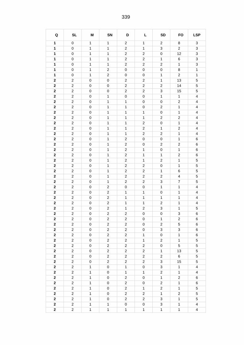
339
Q SL M SN D L SD FO LSP
1 0 1 1 2 1 2 8 3
1 0 1 1 2 1 3 2 3
1 0 1 1 2 2 0 12 3
1 0 1 1 2 2 1 6 3
1 0 1 1 2 2 2 1 3
1 0 1 2 0 0 0 8 1
1 0 1 2 0 0 1 2 1
2 2 0 0 2 2 1 13 5
2 2 0 0 2 2 2 14 5
2 2 0 0 2 2 3 15 5
2 2 0 1 0 0 1 1 4
2 2 0 1 1 0 0 2 4
2 2 0 1 1 0 2 1 4
2 2 0 1 1 1 0 1 4
2 2 0 1 1 1 2 2 4
2 2 0 1 1 2 0 1 4
2 2 0 1 1 2 1 2 4
2 2 0 1 1 2 2 1 4
2 2 0 1 2 0 0 1 6
2 2 0 1 2 0 2 2 6
2 2 0 1 2 1 0 1 6
2 2 0 1 2 1 1 2 6
2 2 0 1 2 1 2 1 5
2 2 0 1 2 2 0 1 5
2 2 0 1 2 2 1 6 5
2 2 0 1 2 2 2 4 5
2 2 0 1 2 2 3 7 5
2 2 0 2 0 0 1 1 4
2 2 0 2 1 1 0 1 4
2 2 0 2 1 1 1 1 4
2 2 0 2 1 1 2 1 4
2 2 0 2 1 2 3 1 5
2 2 0 2 2 0 0 3 6
2 2 0 2 2 0 1 2 6
2 2 0 2 2 0 2 5 6
2 2 0 2 2 0 3 3 6
2 2 0 2 2 1 0 1 6
2 2 0 2 2 1 2 1 5
2 2 0 2 2 2 0 5 5
2 2 0 2 2 2 1 13 5
2 2 0 2 2 2 2 6 5
2 2 0 2 2 2 3 15 5
2 2 1 0 1 0 3 1 4
2 2 1 0 1 1 2 1 4
2 2 1 0 2 0 1 2 6
2 2 1 0 2 0 2 1 6
2 2 1 0 2 1 2 1 5
2 2 1 0 2 2 1 2 5
2 2 1 0 2 2 3 1 5
2 2 1 1 0 0 3 1 4
2 2 1 1 1 1 1 1 4

340
Q SL M SN D L SD FO LSP
1 0 1 1 2 1 2 8 3
1 0 1 1 2 1 3 2 3
1 0 1 1 2 2 0 12 3
1 0 1 1 2 2 1 6 3
1 0 1 1 2 2 2 1 3
1 0 1 2 0 0 0 8 1
1 0 1 2 0 0 1 2 1
2 2 1 1 1 1 3 1 4
2 2 1 1 2 1 3 1 5
2 2 1 1 2 2 1 2 5
2 2 1 1 2 2 2 1 5
2 2 1 1 2 2 3 1 5
2 2 1 2 1 1 0 1 4
2 2 1 2 2 0 1 1 6
2 2 1 2 2 1 0 2 5
2 2 1 2 2 1 3 1 5
2 2 1 2 2 2 0 1 5
2 2 1 2 2 2 1 1 5
2 2 1 2 2 2 2 2 5
2 2 1 2 2 2 3 6 5
2 2 2 0 0 0 0 1 4
2 2 2 0 0 0 1 2 4
2 2 2 0 0 2 3 1 4
2 2 2 0 1 2 0 1 4
2 2 2 0 1 2 1 1 4
2 2 2 0 2 0 0 1 6
2 2 2 0 2 1 0 1 4
2 2 2 0 2 1 2 2 5
2 2 2 0 2 2 0 5 5
2 2 2 0 2 2 1 9 5
2 2 2 0 2 2 2 7 5
2 2 2 0 2 2 3 11 5
2 2 2 1 1 1 1 1 4
2 2 2 1 1 1 2 1 4
2 2 2 1 1 2 0 1 4
2 2 2 1 2 0 0 1 6
2 2 2 1 2 0 2 1 6
2 2 2 1 2 1 0 1 5
2 2 2 1 2 1 3 1 5
2 2 2 1 2 2 0 5 5
2 2 2 1 2 2 1 2 5
2 2 2 1 2 2 2 5 5
2 2 2 1 2 2 3 11 5
2 2 2 2 0 1 0 1 4
2 2 2 2 1 2 2 1 5
2 2 2 2 2 0 0 2 6
2 2 2 2 2 0 1 1 6
2 2 2 2 2 0 2 1 6
2 2 2 2 2 0 3 2 6
2 2 2 2 2 1 0 4 5
2 2 2 2 2 1 1 2 5

341
Q SL M SN D L SD FO LSP
1 0 1 1 2 1 2 8 3
1 0 1 1 2 1 3 2 3
1 0 1 1 2 2 0 12 3
1 0 1 1 2 2 1 6 3
1 0 1 1 2 2 2 1 3
1 0 1 2 0 0 0 8 1
1 0 1 2 0 0 1 2 1
2 2 2 2 2 1 2 1 5
2 2 2 2 2 1 3 1 5
2 2 2 2 2 2 0 6 5
2 2 2 2 2 2 1 12 5
2 2 2 2 2 2 2 13 5
2 2 2 2 2 2 3 17 5

342
8.4 UKHLS pregnant women study
8.4.1 Sleep characteristics
Table 8-19 The seven sleep questions presented in the UKHLS sleep module, and
participants’ responses before and after re-coding
The Seven sleep questions Original responses Responses used in generating sleep clusters
Responses used in running the
regression analysis
Q1: How many hours of
actual sleep did you
usually get at night during
the last month? Note: This
may be different than the
actual number of hours you
spent in bed.
Reported in hours and minutes
1. Reference ( ≥ 6 and ≤ 9 hours)
2. Long sleep (>9 hours) 3. Short sleep (<6 hours)
1. Reference ( ≥ 6 and ≤ 9 hours)
2. Long sleep (>9 hours)
3. Short sleep (<6 hours)
Q2: During the past month, how often have you had trouble sleeping because you Cannot get to sleep within 30 minutes?
1. Not during the past month
2. Less than once a week 3. Once or twice a week 4. Three or more times a
week 5. More than once most
nights
1. Absent (1) 2. Less than three times a
week (2,3) 3. Three or more times a
week (4&5)
1. Absent (1) 2. Present (2,3,4&5)
Q3: During the past month, how often have you had trouble sleeping because you Wake up in the middle of the night or early in the morning?
1. Not during the past month
2. Less than once a week 3. Once or twice a week 4. Three or more times a
week 5. More than once most
nights
1. Absent (1) 2. Less than three times a
week (2,3) 3. Three or more times a
week (4&5)
1. Absent (1) 2. Present (2,3,4&5)
Q4: During the past month, how often have you had trouble sleeping because you Cough or snore loudly?
1. Not during the past month
2. Less than once a week 3. Once or twice a week 4. Three or more times a
week 5. More than once most
nights
1. Absent (1) 2. Less than three times a
week (2,3) 3. Three or more times a
week (4&5)
1. Absent (1) 2. Present (2,3,4&5)
Q5: During the past month, how often have you taken medicine (prescribed or “over the counter”) to help you sleep?
1. Not during the past month
2. Less than once a week 3. Once or twice a week 4. Three or more times a
week
1. Absent (1) 2. Less than three times a
week (2,3) 3. Three or more times a
week (4)
1. Absent (1) 2. Present (2,3 & 4)
Q6:During the past month, how often have you had trouble staying awake while driving, eating meals, or engaging in social activity?
1. Not during the past month
2. Less than once a week 3. Once or twice a week 4. Three or more times a
week
1. Absent (1) 2. Less than three times a
week (2,3) 3. Three or more times a
week (4)
1. Absent (1) 2. Present (2,3 & 4)
Q7: During the past month, how would you rate your sleep quality overall?
1. Very good 2. Fairly good 3. Very bad 4. Fairly bad
1. Good (1&2) 2. Bad (3&4)
1. Good (1&2) 2. Bad (3&4)

343
8.4.2 Coding of pregnancy variables presented in the UKHLS data set
Table 8-20 Detailed coding of pregnancy variables identified within the UKHLS.
Pregnancy-related variable
Variable in Wave 2 Variable in Wave 5 Original coding Coding used in the analysis
Caesarean section b_pregout1 “outcome of pregnancy”
e_pregout1 “outcome of pregnancy”
1.Live birth – caesarean
2.Live birth - normal delivery
3.Not live birth
Delivered by caesarean section
0.No (live birth - normal delivery)
1.Yes (live birth - caesarean) Participants responded by “Not live birth” were excluded
Birth weight b_bwtoz “birth weight in ounces” e_bwtoz “birth weight in ounces” In ounces Had a macrosomic baby 0.No 1.Yes Had a low birth baby 0.No 1.Yes b_bwtk “birth weight in kg” e_bwtk “birth weight in kg” In grams
b_bwtlb “birth weight in pounds” e_bwtlb “birth weight in pounds” In pounds
Preterm delivery b_bwtxp “was CHILD'S NAME born within one week of the expected due date?”
e_bwtxp “was CHILD'S NAME born within one week of the expected due date?”
0.Yes
1.No
Had preterm delivery 0.No 1.Yes
b_bwte “was CHILD'S NAME child born early or late”
e_bwtel “was CHILD'S NAME child born early or late”
1.Early 2.Late
b_bwtwk “How many weeks early/late”
e_bwtwk “How many weeks early/late” Weeks
Alcohol consumption
b_pregdrink1 “drank alcohol during pregnancy”
e_aedrof1 “which of these best describes how often you usually drank alcohol during this pregnancy?”
1.Never drank any alcohol 2.Less than 1-2 pw or occasion, 3.Equal to 3-6 pw or 3-5 per occasion 4.7+ pw/6+ per occasion
Drunk alcohol during pregnancy 0.No 1.Yes
Smoking b_pregsmoke1 “smoked during pregnancy”
e_pregsmoke1 “smoked during pregnancy”
0.Yes
1.No
Smoked during pregnancy 0.No 1.Yes

344
8.4.3 Coding of confounders presented in the UKHLS dataset
Table 8-21 Detailed coding of covariates identified as confounders within the UKHLS.
Confounder Variable in Wave 1 Variable in Wave 4 Original coding Coding used in the analysis
Ethnicity a_racel_dv “ethnic group”
d_racel_dv “ethnic group” 1.White (British, Irish, Gypsy or Irish traveller, other) 2.Mixed (White and Black African, White and Black
Caribbean, White and Asian, Other mixed) 3.Asian (Indian, Pakistani, Chinese, Other) 4.Black (African, Caribbean, Other Black) 5.Others (Arab, Other)
1.Ethnicity with lower risk of GDM (White)
2.Ethnicity with higher risk of GDM (Other ethnic groups)
Employment a_jbstat “Please look at this card and tell me what best describes NAME's current employment situation?”
d_jbstat “Please look at this card and tell me what best describes NAME's current employment situation?”
1.Unemployed (unemployed, looking after family or home) 2.Self-employed (self-employed, unpaid worker in family
business, doing something else) 3.Employed (paid employment (F/T, P/T)) 4.Sick /disabled (on maternity leave, long-term sick or
disabled) 5. F/T training or education (on a government training
scheme, F/T student)
0.Working at the time of the interview (employed, self-employed)
1.Not working at the time of the interview (Unemployed, Sick /disabled, F/T training or education)
Cohabitation a_mlstat_dv “What is your current legal marital status? Are you…”
d_mlstat_dv “What is your current legal marital status? Are you…”
1.Single, never married/in civil partnership 2.Married 3.Civil partner 4.Separated from spouse 5.Divorced
0.Living as couple (married, civil partner)
1.Not living as a couple (single, never married/in civil partnership, divorced, separated from spouse)
Education a_hiqual_dv “Highest educational qualification”
d_hiqual_dv “Highest educational qualification”
1.Degree
2.Other higher
3.A level etc.
4.GCSE etc.
5.Other qualification
6.No qualification
1.Degree or higher (degree, other higher)
2.A level and less (A level etc., GCSE etc., other qualification, no qualification)
Medical condition
a_hconds “Do you still have…”?
d_hconds “Do you still have HCond”?
96. None of these 1. Asthma 2. Arthritis 3. Congestive heart failure 4. Coronary heart disease 5. Angina 6. Heart attack or myocardial infarction 7. Stroke 8. Emphysema 10. Hypothyroidism or an under-active thyroid 11. Chronic bronchitis 12. Any kind of liver condition 13. Cancer or malignancy 14. Diabetes
Does the participant had one of the following chronic medical condition (i.e. cardiovascular, neurological, psychological, metabolic, inflammatory)? 1. No 2. Yes

345
Confounder Variable in Wave 1 Variable in Wave 4 Original coding Coding used in the analysis
15. Epilepsy 16. High blood pressure 17. Clinical depression 9. Hyperthyroidism or an over-active thyroid
Parity a_lprnt “Ever had/fathered children”
d_lnprt “Ever had/fathered children”
1.Yes 2.No
Parity
0.Nulliparous
1.Multiparous
a_lnprnt “Number of biological children ever had/fathered”
d_lnprnt “Number of biological children ever had/fathered”
Numbers
a_nchild_dv “Number of own children in household”
d_nchild_dv “Number of own children in household”
Numbers
Household composition
a_hhtype_dv Classification follows closely the household composition classification in the Labour Force Survey
d_hhtype_dv Classification follows closely the household composition classification in the Labour Force Survey
0.1 male, aged 65+, no children,
1.1 female, age 60+, no children,
2.1 adult under pensionable age, no children
3.1 adult, 1 child
4.1 adult, 2 or more children
5.Couple both under pensionable age, no children
6.Couple 1 or more over pensionable age, no children
7.Couple with 1 child
8.Couple with 2 children
9.Couple with 3 or more children
10.3 or more adults, no children, incl. at least one couple
11.3 or more adults, 1-2 children, incl. at least one couple
12.3 or more adults, >2 children, incl. at least one couple
13.2 adults, not a couple, both under pensionable age, no children
14.2 adults, not a couple, one or more over pensionable age, no children
15.3 or more adults, no children, excl. any couples
16.2 adults, not a couple, 1 or more children
17.3 or more adults, 1 or more children, excl. any couples
0.Single without children (reference)
1.Single with children
2.Couple with children
3.Couple without children

346
8.4.4 Missing data
Table 8-22 Distribution of sleep characteristics amongst women with complete and missing data on pregnancy outcomes in the UKHLS (n = 921).
Participants with missing
birth outcomes
Participants with
complete birth outcomes
n=376 % n=545 %
Sleep duration < 6 hours 272 72.34 387 71.01
6 to 9 hours 39 10.37 67 12.29
> 9 hours 22 5.85 33 6.06
Missing 43 11.44 58 10.64
Latency Absent 127 33.78 186 34.13
Present 206 54.79 303 55.6
Missing 43 11.44 56 10.28
Disturbance Absent 127 33.78 75 13.76
Present 206 54.79 414 75.96
Missing 43 11.44 56 10.28
Snoring or
coughing
Absent 256 68.09 370 67.89
Present 73 19.41 108 19.82
Missing 47 12.5 67 12.29
Day sleepiness Absent 282 75 410 75.23
Present 50 13.3 75 13.76
Missing 44 11.7 60 11.01
Medication Absent 319 84.84 467 85.69
Present 21 5.59 29 5.32
Missing 36 9.57 49 8.99
Quality Good 226 60.11 363 66.61
Bad 115 30.59 134 24.59
Missing 35 9.31 48 8.81
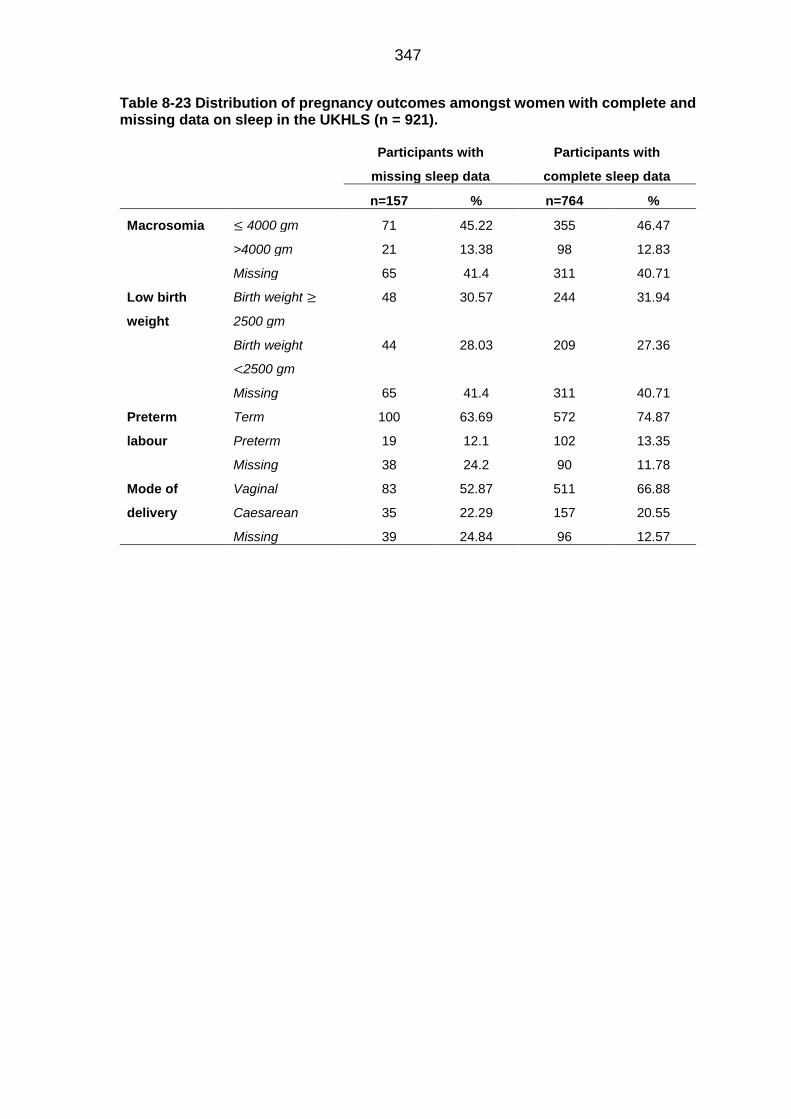
347
Table 8-23 Distribution of pregnancy outcomes amongst women with complete and missing data on sleep in the UKHLS (n = 921).
Participants with
missing sleep data
Participants with
complete sleep data
n=157 % n=764 %
Macrosomia ≤ 4000 gm 71 45.22 355 46.47
>4000 gm 21 13.38 98 12.83
Missing 65 41.4 311 40.71
Low birth
weight
Birth weight ≥
2500 gm
48 30.57 244 31.94
Birth weight
<2500 gm
44 28.03 209 27.36
Missing 65 41.4 311 40.71
Preterm
labour
Term 100 63.69 572 74.87
Preterm 19 12.1 102 13.35
Missing 38 24.2 90 11.78
Mode of
delivery
Vaginal 83 52.87 511 66.88
Caesarean 35 22.29 157 20.55
Missing 39 24.84 96 12.57

348
Table 8-24 Distribution of sociodemographic and health characteristics of women with complete and missing data on sleep or pregnancy outcomes in the UKHLS (n = 921).
Missing sleep or
medical data
Complete sleep and
medical data
n=468 % n=453 %
Age ≤ 19 years 14 2.99 13 2.87
20-29 years 129 27.56 102 22.52
30-39 years 129 27.56 106 23.4
≥ 40 years 28 5.98 9 1.99
Missing 168 35.9 223 49.23
Parity Nulliparous 261 55.77 312 68.87
Multiparous 207 44.23 141 31.13
Missing 0 0 0 0
Ethnicity Lower risk of GDM 342 73.08 351 77.48
Higher risk of GDM 124 26.5 99 21.85
Missing 2 0.43 3 0.66
Cohabitation Not cohabited 66 14.1 108 23.84
Cohabited 402 85.9 344 75.94
Missing 0 0 1 0.22
Smoking Not current smoker 309 66.03 379 83.66
current smoker 48 10.26 74 16.34
Missing 111 23.72 0 0
Alcohol No alcohol consumption 287 61.32 345 76.16
Alcohol consumption 71 15.17 108 23.84
Missing 110 23.5 0 0
Employment Currently working 25 5.34 32 7.06
Currently not working 270 57.69 278 61.37
Missing 173 36.97 143 31.57
Education Degree and higher 234 50 219 48.34
A level and Lower 196 41.88 196 43.27
Missing 38 8.12 38 8.39

349
8.5 Association between sleep variables and pregnancy
outcomes in participants at risk of GD
8.5.1 Ethical approval letter for the Scott/Ciantar study.

350

351

352
8.5.2 Data extraction method
8.5.2.1 Identifying the study’s variables
The existing published literature was searched, and clinicians were consulted to
identify potential key variables that might play a role in the association between
sleep and pregnancy outcomes. The potential variables were then assessed for
their availability in the medical records used at Leeds Teaching Hospitals NHS
Trust.
In this stage, a simple hypothetical directed acyclic graph (DAG) was drawn to
anticipate the key variables to extract (Figure 6-2). The variables were arranged
according to their temporal sequences (i.e., when the ‘event’ or ‘process’ these
variables represented had occurred in the pregnancy). Their suggested
relationships were symbolised using unidirectional arrows. From the hypothetical
DAG (Figure 6-2), the priority variables were assigned to be the pre-pregnancy
events and individual features (e.g., pre-pregnancy weight, previous pregnancies
history and SES), possible confounders from the early pregnancy events (e.g.,
multiple pregnancies) and outcomes of interest (e.g., maternal and neonatal
complications). Late pregnancy events were considered proxies for sleep and were
not set as priority variables (e.g., GHTN, PE and foetal distress).
Figure 8-6 Hypothetical directed acyclic graph showing the temporal relationship amongst variables likely to have been available for participants the Scott/Ciantar study

353
If a variable was not available in the records, its proxy was gathered instead. For
example, a postcode was used instead of socioeconomic status, and the booking
weight at the first antenatal visit was used instead of the pre-pregnancy weight.
Each medical file consisted of the following records:
Antenatal records: personal information, health information, family history,
obstetric history, anthropometric data, midwife and physician notes, laboratory
records and ultrasound records
Birth records: personal information, current pregnancy complications, admission
details, birth details, new-born records and discharge summary
Diabetic antenatal clinic records: physician notes
Each variable was given a reference number and then plotted against the record's
name and the page number in that record to create a guide for the extractors.
When all the variables of interest were identified, a detailed DAG was generated.
The available variables were then arranged according to their temporal sequence.
A DAG was drawn using the available variables to identify those that might be
confounders, mediators or competing exposures in each possible (and available)
specified outcome.
8.5.2.2 Collecting data from the clinical records
Before the data were collected, the following criteria were established:
I. Only variables required for adjustment in any analyses between sleep and
each pregnancy outcome were extracted from the medical records (an
approach that was intended to increase the efficiency of data extraction).
II. The data for each extracted variable were examined for quality (i.e.,
precision, consistency, accuracy and missingness), and only variables of
acceptable quality were considered for inclusion in the analysis.
III. Data were collected at the end of the pregnancy period first from the hard
copy of the record. If missingness was encountered, the missing data were
searched for in the online records available in the library. The medical
records were inspected carefully, and the extracted data were transferred
to an Excel sheet as follows:
First, the information was reported on the Excel sheet exactly as it was written in
the records (e.g., neonatal complications at birth were written on the Excel sheet
as they were in the records before deriving the NICU admission and prematurity
variables from the details). Subsequently, coding took place after revising the
gathered data.

354
The objectively measured variables (e.g., weight) were reported on the Excel sheet
as they were recorded by health professionals in the medical records in numbers
and units. The units were converted into a single unified unit when the quality of
the variable was determined.
If a variable (e.g., maternal age) was reported in different locations in the records
(e.g., in the personal information sheet, in the first antenatal visit sheet and in the
labour information sheet), all these data were gathered and reported separately in
several columns in Excel to examine their consistency and to compensate for
missingness in one location.
In recording medical diagnoses, objective measurements were used to confirm the
diagnosis instead of subjective measurements (e.g., depending on US to diagnose
large for gestational age foetus (LGA) and not fundal height).
The participants’ medical records were handled securely within the Trust’s
premises. The extracted data were stored on a secure (password-protected) hard
drive at the university, which only authorised personnel were able to access. No
personal identification data (names, complete address and complete NHS number)
were recorded, as each participant was given a unique study identification number.
8.5.2.3 Data cleaning and coding
The data were carefully gathered from medical records and then transcribed on an
Excel sheet without modifying or paraphrasing sentences or words. These data
were then revised for recoding according to the following criteria:
Continuous variables that acted as confounders and required adjustment in the
regression models (e.g., maternal BMI and age) were kept continuous whereas the
continuous variables that were chosen as outcomes (i.e., weeks of gestation, birth
weight, Apgar score and estimated blood loss) were transformed into binaries to
estimate the odds ratio.
Categorical variables were recoded as binary variables to reduce the number of
categories, which allowed us to increase the number of adjusted confounders
without losing the stability of the regression models.
Variables with open details (e.g., neonatal transferred details or labour ward
admission details) were used in one of two ways:
To examine the consistency of other variables, such as the labour ward admission
details, including a summary of current pregnancy complications, which was used
to examine the consistency of development of LGA or current GDM.

355
Generating new variables according to yes or no responses. For example,
transferred neonatal details and discharge summaries were both used to generate
an NICU admission variable that had a yes or no response.
(Table 8-25) presents a detailed summary of the extraction and coding of each
variable.

356
Table 8-25 Details of data extracted from the medical records for use as analytical variables in the Scott/Ciantar study.
Variable name Medical records Section Question Original coding New coding
Birth weight Birth records
New-born details
“Birth weight “ Grams Low birth weight
0.No
1.Yes
Macrosomia
0.No
1.Yes
Preterm Birth records
1. New-born details 2. Admission to the delivery ward details
“Weeks of gestation” Weeks Preterm
0.No
1.Yes
Caesarean delivery
Birth record 1. Caesarean delivery details 2. Discharge summary
Mode of delivery • Normal vaginal delivery
• Forceps assessed vaginal delivery
• Emergency caesarean delivery
• Elective caesarean delivery
Caesarean delivery 1. No 2. Yes
Estimated blood loss
Birth records Delivery details
“Estimated blood loss”
Continuous variable Blood loss >500 ml
0.No
1.Yes
3rd degree tear or more
Birth records Delivery details
“Degree of tear” • First
• Second
• Third
• Fourth
0.Absent (first, second)
1.Present (third, fourth)
Apgar scores Birth records
New-born details
“0 minutes Apgar’s score” and “5 minutes Apgar’s score”
Scale from 0 to 10
Low Apgar score <7
0.No
1.Yes
NICU admission Birth records
1. New-born details 2. Discharge summary
“Transfer, details” Open ended response Admitted to NICU 0.No 1.Yes
Previous GDM Antenatal records
Health problems
“Have you ever had any of the following -diabetes”
Yes or no responses plus details Previous history of GDM 0.No 1.Yes Obstetric history
“Previous pregnancies details” -“any problems during pregnancy”
Yes or no responses plus details
Midwife notes
It was mentioned as risk factors of GDM and causes of OGTT referral
Open ended response
Diabetic antenatal clinic records
Physician notes in the first visit It was mentioned as risk factors of GDM
Open ended response

357
Variable name Medical records Section Question Original coding New coding
Family history of DM
Antenatal records Family history details “Does anyone in your family have any of the following-Diabetes
Yes or no responses plus details Family history of DM
0.No
1.Yes Midwife notes
It was mentioned as risk factors of GDM and causes of OGTT referral
Open ended response
Diabetic antenatal clinic records
Physician notes in the first antenatal visit
It was mentioned as risk factors of GDM
Open ended response
History of previous macrosomia
Antenatal records Obstetric details
“Previous pregnancies details”-birth weight
1.Yes 2.No
Previous history of macrosomia
0.No
1.Yes
Midwife notes It was mentioned as risk factors of GDM and causes of OGTT referral
Open responses
Diabetic antenatal clinic records
Physician notes in the first visit It was mentioned as risk factors of GDM
Obstetric history
Antenatal records
Obstetric history details “Previous pregnancies details”- “any problems: during pregnancy, labour and birth and after birth”
Yes or no response plus details 0. Non-significant obstetric history 1.Significant obstetric history (Miscarriages before 12 weeks, Miscarriages after 12 weeks, Still births, Caesarean sections, Birthweight under 2.5 kg, and Gestation under 37 weeks)
Obstetric summary; 1.Miscarriages before 12
weeks 2.Miscarriages after 12 weeks 3.Still births 4.Caesarean sections 5.Birthweight under 2.5 kg 6.Gestation under 37 weeks
1.Yes 2.No
Gender of the new-born
Birth records New-born details “gender of the new-born”
1. Male 2. Female
0.No 1.Yes
OGTT test results
Antenatal records For women with or without GDM, it was reported from the lab investigation results
Two readings; fating and 2 hours post prandial
Mmol/l Continuous variable
For women with GDM, it was reported from the physician notes in the first diabetic antenatal clinic
Two readings were recorded; fating and 2 hours post prandial
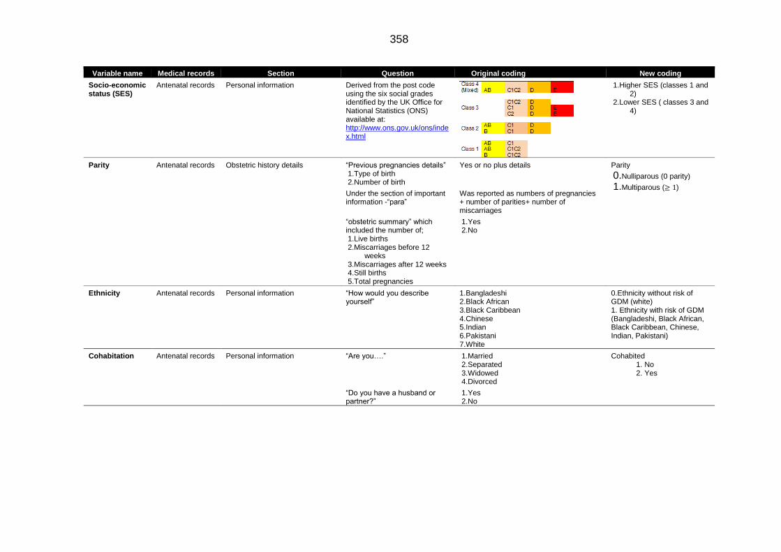
358
Variable name Medical records Section Question Original coding New coding
Socio-economic status (SES)
Antenatal records Personal information Derived from the post code using the six social grades identified by the UK Office for National Statistics (ONS) available at: http://www.ons.gov.uk/ons/index.html
1.Higher SES (classes 1 and 2)
2.Lower SES ( classes 3 and 4)
Parity Antenatal records Obstetric history details “Previous pregnancies details” 1.Type of birth 2.Number of birth
Yes or no plus details
Parity
0.Nulliparous (0 parity)
1.Multiparous (≥ 1) Under the section of important information -“para”
Was reported as numbers of pregnancies + number of parities+ number of miscarriages
“obstetric summary” which included the number of; 1.Live births 2.Miscarriages before 12
weeks 3.Miscarriages after 12 weeks 4.Still births 5.Total pregnancies
1.Yes 2.No
Ethnicity Antenatal records Personal information “How would you describe yourself”
1.Bangladeshi 2.Black African 3.Black Caribbean 4.Chinese 5.Indian 6.Pakistani 7.White
0.Ethnicity without risk of GDM (white) 1. Ethnicity with risk of GDM (Bangladeshi, Black African, Black Caribbean, Chinese, Indian, Pakistani)
Cohabitation Antenatal records
Personal information “Are you….”
1.Married 2.Separated 3.Widowed 4.Divorced
Cohabited 1. No 2. Yes
“Do you have a husband or partner?”
1.Yes 2.No

359
Variable name Medical records Section Question Original coding New coding
Medical condition
Antenatal records Health information “Have you ever had any of the following….” • Anaesthetic problem
• Asthma or chest problems
• Blood transfusion
• Diabetes
• Epilepsy
• Fertility problems
• Vaginal infections
• Heart problems
• High blood pressure
• Kidney or urinary problems
• Liver disease or hepatitis
• Mental health problems
• Operations
• Physiological difficulties
• Thrombosis
•
Health condition
0.No
1.Yes
Smoking Antenatal records
Health details Have you ever smoked 1.Yes 2.No
Current smoker
0.No
1.Yes “When did you stop smoking” Date
“Number of cigarettes smoked a day”
Number
Alcohol Antenatal records
Health details “Do you drink alcohol” 1.Yes 2.No
Drinking alcohol during current pregnancy
• No
• Yes
“How many units of alcohol do you drink each week?”
Number
BMI in the first antenatal visit
Antenatal records
Anthropometry details “Important information-BMI “
Kilogram /meter2 • Underweight <18.5
• Normal <25 & ≥ 18.5
• Overweight <30 &≥ 25
• Obese ≥ 30
Maternal age Antenatal records
Personal information Age Years Years
Midwife notes
Diabetic antenatal clinic
Birth records Admission details

360
8.5.3 Quality of variables extracted from the medical records
Table 8-26 Quality of the variables extracted from the medical records of participants who were included in the Scott/Ciantar study, according to their accuracy, consistency and precision.
Variables Recording method Accuracy Consistency Precision
Age Recorded by the midwife
during the first antenatal visit.
Age in the first visit antenatal was chosen to
be included in the analysis, as it preceded all
events of interest. There was a slight
difference between it and the age when the
questionnaire was collected, and medical data
were gathered (few months).
It was consistent compared to the date of
birth.
Because it was reported in years, the
level of precision was less than if it had
been reported in months.
Postcode and
derived SES
Recorded by the midwife
during the first antenatal visit.
It was accurate because it was crucial
information, and it was updated for each visit.
SES information was estimated using the
postcode based on the six social grades
invented by the UK Office for National
Statistics (ONS):
http://www.ons.gov.uk/ons/index.html
It was consistent compared with the
patient identification information
presented in the identification slip.
The derived level of SES was not
precise, as it projected a rough
estimation based on the postcode only
and not on all the indicators of SES
(e.g., education, job and income).
Estimation using postcode gives an
idea about the neighbourhood rather
than a particular household.
Ethnic group Reported by the participants Participants occasionally were mistaken about
their ethnicity with other measurements. As a
result, rather than choosing one of the
available categories, they wrote their
understanding of ethnicity, which in some
cases was their religion (e.g., Sikh) or
nationality (e.g., British, Iranian and Chinese)
In the case of religion, ethnicity was coded as
missing, and in the case of nationality,
ethnicity was coded as appropriate.
No other records to compare The categories were both broad and
limited, and they depended on the
participants’ statement of their ethnic
origin.
The number of categories was further
reduced during the analysis, and the
focus was directed to categorising
ethnicity based on the associated risk
of developing GDM and not on the
precise ethnic groups.
Marital status Reported by the participants Having both limited and broad categories
might have affected the accuracy of the
variables. For instance, some participants did
not choose a response from the available
choices but described their status as engaged
or widow, for example.
Consistent with the partnership variable The martial status might change over
the course of pregnancy, which might
affect the precision if it was not
updated in the medical notes.
However, because the interest was not
the legal status but the presence of a

361
Variables Recording method Accuracy Consistency Precision
In a later stage, this variable was merged with
the partnership variable to compensate for
missingness in both variables. It was termed
cohabiting and categorised as a binary.
partner, the variable was used to
generate a new variable, which was
the presence of a partnership.
Partnership Reported by the participants Reported as either yes or no without further
details. However, in a later stage, this variable
was merged with the marital status variable to
compensate for missingness in both variables.
Consistent with the marital status
History of
smoking
Reported by the participants Few participants reported the date that they
had quit smoking as the date of their first
antenatal visit. If the patient reported the date
she stopped smoking as the date of the first
antenatal visit or within the last week, the
participant was considered a current smoker.
In the beginning, four groups were defined
(i.e., current smoker, ex-smoker, passive
smoker and never smoked), but because of
the small number of participants in each
group, it was further reduced to either current
smoker or not a current smoker, which caused
a further loss of information and deceased the
level of accuracy
The history of smoking was derived from
three questions in the records.
1.Have you ever smoked: (yes, no)?
2.Date stopped smoking: _/_/_
3.Number of cigarettes per day: ___
4.Does your partner smoke?
Using word “ever” in the question made it
difficult to understand the current smoking
status of a participant especially if not all
the three questions were answered by
her.
E.g., a participant might respond by
choosing yes for the first question then
leaving the rest empty, which made it
unclear if she still smoked or had stopped.
Measurement of smoking only once in
early pregnancy and the use of yes
and no responses might not be a
precise reflection of the smoking status
because it might change during
pregnancy, as well as the number of
cigarettes and the amount of inhaled
smoke.
Alcohol Reported by the participants Participants might not be accurate about
reporting their consumption status and the
amount of alcohol they consumed. In addition,
some participants did not respond to the
question, which might be linked to their
unwillingness to divulge the consumption of
alcohol.
The variable was reduced later in the analysis
to yes or no. This reduction caused the loss of
much information.
Compared with the unit per week variable Measurement of alcohol consumption
only once in early pregnancy and the
use of yes and no responses might not
be a precise reflection of the drinking
status, which might change during
pregnancy, as well as the number of
consumed units.

362
Variables Recording method Accuracy Consistency Precision
Family history of
DM
Reported by the participants Reported by participants as yes or no Compared with the risk factor of
gestational diabetes recorded in notes by
the midwife and physician, which were
consistent
Precision depended on the reliability of
the participant.
DM in first
degree relative
Reported by the participants If a participant mentioned that her mother,
father, sister or brother had a history of
diabetes, the response was considered yes.
However, many participants neglected to
indicate who had a history of DM.
Compared with the risk factors of
gestational diabetes in the notes by the
midwife and physician, which were
consistent
Precision depended on the reliability of
the participant.
History of
previous GDM
Reported by the participants The accuracy depended on the accuracy of
the participants.
Compared with the following variables:
history of DM, risk factor of GDM and
previous pregnancy complications, which
were consistent
Precision depended on the reliability of
the participant.
BMI Measured by the midwife
during the first antenatal visit
Calculated by the midwife and reported
rounder up to different decimal numbers
Compared with the risk factors of GDM in
the notes by the midwife and physician;
the height and weight
The precision depended on the
precision of the measured weight,
which was determined by different
scales in different settings and different
health professionals.
These different situations might have
affected the level of precision.
Parity Recorded by the midwife
during the first antenatal visit
Reported based on a given history, so the
accurately depended on the participant.
Parity indicated birth and did not reflect in full
what happened with previous pregnancies
such as miscarriages after 12 weeks and
before 20 weeks, which might limit the
accuracy of this variable in influencing the
association between sleep and pregnancy
outcomes. In addition, it did not till details of
multiple pregnancies
Compared with the number of previous
pregnancies, the number of still or live
births and the number of miscarriages,
inconsistent reporting was found,
especially in the number of previous
pregnancies and parity. Perhaps the
inconsistency was linked to the
understanding of a midwife of how to
report the variable, which should be
reported in the following format:
P = number of pregnancies + number of
deliveries after 20 + terminated
pregnancy before 20 weeks
Precision depended on the reliability of
the participant

363
Variables Recording method Accuracy Consistency Precision
Previous
obstetric
complications
Recorded by the midwife
during the first antenatal visit.
Derived from details of previous pregnancies
and the numbers of still births, live births,
miscarriages, caesarean deliveries, neonatal
deaths and low birth weights
Reported based on the history given by the
participant, so its accuracy depended on the
participant. In addition, as midwives did not
provide information, we had trace them to
other locations in the records, which might
have affected the accuracy of the variable,
especially in relation to events occurring
before or after 12 weeks of gestation.
Previous obstetric complications was
categorised as the presence or absence of
complications, which led to the loss of
information.
Variables used to generate this variable
were examined against each other.
Inconsistency was found between the
reported numbers, the details of previous
pregnancies and the reported parity.
Large amounts of missingness were also
found in the number of previous obstetric
events.
Precision depended on the reliability of
the participant
OGTT results Reported as lab test results
on the lab paper slip or in the
first visit to the diabetic
antenatal clinic.
Reported in mmol/l as fasting and 2 hours
postprandial. The numbers were
approximated to the second decimal point.
Many factors might affect the precision
of the readings, e.g. fasting of the
participants, accurate 2 hours period
between the two readings and GA
Repeating the reading might not give
similar result if repeated in different
circumstances.
Gestational age
when delivery
occurred
Recorded by the midwife
based on the early ultrasound
Reported in weeks and days. However,
because it was reported based on an early
ultrasound, there is still some chance of error
of one week or two.
Subsequently, the variable was divided into
term and preterm (< 37 weeks)
Compared with the birth plan in the
diabetic antenatal care notes for women
with GDM and with the notes of the
midwife for the last antenatal visit for
women without GDM. It also was
compared with early ultrasound records
and neonatal birth details, which were
consistent.
Depended on the Ultrasound machine
and the technician as different sitting
might lead into a different result
However, the result was compared
with last menstrual period and fundal
height and sometimes 4 weeks
different was noticed

364
Variables Recording method Accuracy Consistency Precision
Mode of delivery Recorded by the midwife
after birth
It was sometimes not reported as an
emergency or an elective caesarean delivery,
especially in the online records.
Because of the lack of consistency and
accuracy in reporting the instrumental delivery
and the reasons for caesarean, the variable
was categorised as a caesarean delivery or a
vaginal delivery without further details.
Compared with previous obstetric history
for emergency caesarean and elective
caesarean, as well as the number of
previous caesareans, which were
consistent.
Also compared with neonatal
complications and US records for breach
presentation, which were consistent.
Estimated blood
loss
Recorded by the midwife
after birth
It depended on the midwife’s estimation, so it
was not an accurate measurement.
It was examined against discharge
summary details, and it was consistent.
The precision was low since it was
depended on the estimation and
different midwives
Birth weight Recorded by the midwife
after birth
Birth weight was measured by the midwife
immediately after birth using a neonatal scale.
Hence, the accuracy of the variable depended
on the accuracy of the scale. The birth weight
was reported in grams. However, the analysis
generated two variables.
Macrosomia (birth weight > 4,000 g) and LBW
(birth weight < 2,500 g). As a result some
information was lost.
Compared with the following variables:
estimated foetal weight in the last
ultrasound; neonatal complication; the
indication of NICU admission; prematurity
records; and presence of twin pregnancy
A good level of consistency was found.
The weight was taken by different
scale in different setting by different
health professionals which might
affected precision
Gender
Recorded by the midwife
after birth
NICU admission Recorded in the transfer
records by the midwife
The reasons for NICU admission were varied
(e.g., prematurity and genetic anomalies);
dividing the responses into yes or no led to
the loss of valuable information.
Compared with the following variables:
neonatal complication: prematurity,
gestational age, multiple pregnancies,
mode of delivery and foetal growth. The
variables were consistent.

365
8.5.4 Missing data
8.5.4.1 Mechanisms of missingness of missing data
Of the 193 participants who were successfully recruited at the beginning of the
study, the files of 15 participants were lost at the end of the study, and their
medical data were not gathered (Figure 8-7). The reasons for the loss of the
medical records are the following:
I. Medical files were lost in another department
II. Medical files were transformed into online records and could not be accessed.
III. Participants delivered outside Leeds, and their medical files were transferred to another NHS trust.
Only 127 of the remaining 178 participants with accessible medical records had
complete medical records of the outcomes of interest (i.e., delivery mode, blood
loss, preterm delivery, birth weight, NICU admission and Apgar score) and the
covariates (i.e., age, race, alcohol, smoking, BMI, age, SES, parity, sex of the
neonate, health condition, partner and OGTT results; Figure 8-8). In dividing the
number of accessible medical records by the number complete medical records,
we found the completion rate of the medical records to be 71.34%.

366
Figure 8-7 Flow chart summarising the numbers and mechanisms of missingness of the lost medical records for Scott/Ciantar study participants whose medical records could not be located.

367
Figure 8-8 Flow chart summarising the numbers and mechanisms of missingness of missing clinical medical data amongst Scott/Ciantar study participants.

368
Of the 193 participants who were recruited in the study, nine participants did not
return their sleep questionnaires. However, two participants without questionnaires
were excluded because they did not fit the inclusion criteria (Figure 8-9). Nineteen
of the 180 women who returned their questionnaires did not respond to some
questions (Figure 8-9).
The completion rate of the sleep questionnaire was 162 (the number of participants
who responded to all questions), which was divided by 180 (the number of
participants who returned their questionnaire) and then multiplied by 100 = 85.56%.
Figure 8-9 Flow chart summarising the numbers, and mechanisms, of missing sleep data for the Scott/Ciantar study participants.
The number of participants who completed the sleep questionnaire and who had
complete medical data was 108: completion rate = (108/187) x 100 = 57.4 %.
(Figure 8-10).

369
Figure 8-10 Summary of the number of participants in the Scott/Ciantar study with complete medical and sleep data.
8.5.4.2 Number and characteristics of missing data
Table 8-27 Socio-demographic features of participants with missing sleep data compared to those of participants with complete sleep data in the Scott/Ciantar study (N = 187)
Missing sleep data Complete sleep data
n=25 % n=162 %
Age ≤ 19 years 1 4 4 2.47 20-29 years 10 40 58 35.8 30-39 years 12 48 91 56.17 ≥ 40 years 2 8 9 5.55 Missing 0 0 0 0
Parity Nulliparous 8 32 67 41.36 Multiparous 15 60 84 51.85 Missing 2 8 11 6.79
SES Higher class 6 24 62 38.27 Lower class 17 68 96 59.26 Missing 2 8 4 2.47
Ethnicity Lower risk of GDM 6 24 32 19.75 Higher risk of GDM 16 64 113 69.75 Missing 3 12 17 10.49
Cohabitation Not cohabited 3 12 11 6.79 Cohabited 19 76 138 85.19 Missing 3 12 13 8.02
Smoking Not current smoker 18 72 116 71.6 Current smoker 4 16 16 9.88 Missing 3 12 30 18.52
Alcohol No alcohol consumption 17 68 116 71.6 Alcohol consumption 4 16 21 12.96 Missing 4 16 25 15.43
BMI Underweight 0 0 0 0 Normal weight 6 24 37 22.84 Overweight 6 24 46 28.4 obese 10 40 65 40.12 Missing 3 12 14 8.64

370
Table 8-28 Frequency distribution of birth outcomes amongst participants with missing
sleep data compared to those of participants with complete sleep data in the Scott/Ciantar
Scott/Ciantarstudy (N = 187)
Missing sleep data Complete sleep data
n=25 % n=162 %
EBL ≥ 500 ml 15 60 105 64.81
<500 ml 10 40 57 35.19 Missing 0 0 0 0
Low birth weight
Birth weight ≥ 2500 gm 25 100 142 87.65
Birth weight <2500 gm 0 0 7 4.32
Missing 0 0 13 8.02 Apgar at birth ≥ 7 23 92 147 90.74
<7 2 8 15 9.26 Missing 0 0 0 0
Preterm labour Term 24 96 146 90.12 Preterm 0 0 8 4.94 Missing 1 4 8 4.94
Mode of delivery
Vaginal 16 64 103 63.58 Caesarean 8 32 49 30.25 Missing 1 4 10 6.17
NICU admission
No admission 24 96 136 83.95 Admission 1 4 9 5.56 Missing 0 0 17 10.49
The frequency distribution of sleep characteristics in the participants with missing
data was similar to the distribution of characteristics in those with complete data
(Table 8-29).
The sleep duration of participants with missing data was mainly within the
reference range (75%, n= 45). Latency (70.97%, n= 44) and disturbance (93.55%,
n = 58) tended to be present, whereas the usage of medication (3.23%, n=2) and
snoring (25.8%, n=116) were almost absent. Quality was reported as good to fairly
good (54.84%, n= 34) and day sleepiness (59.68%, n= 37) was absent in
approximately half of these participants.
Table 8-29 Frequency distribution of sleep characteristics amongst participants in the
Scott/Ciantar study who had complete and missing medical data (N = 187)
Participants with missing medical data
Participants with complete medical data
n=62 % N=125 %
Sleep duration
Short sleep (<6) 10 16.13 23 18.4 Reference range (6-9) 45 72.58 74 59.2 Long sleep (>9) 4 6.45 20 16 Missing 3 4.84 8 6.4
Latency Absent 15 24.19 36 28.8 Present 44 70.97 81 64.8 Missing 3 4.84 8 6.4
Disturbance Absent 1 1.61 12 9.6 Present 58 93.55 105 84 Missing 3 4.84 8 6.4
Snoring or coughing
Absent 42 67.74 75 60
Present 16 25.81 42 33.6 Missing 4 6.45 8 6.4
Day sleepiness
Absent 37 59.68 78 62.4
Present 20 32.26 38 30.4 Missing 5 8.06 9 7.2
Medication Absent 55 88.71 114 91.2

371
Participants with missing medical data
Participants with complete medical data
n=62 % N=125 % Present 2 3.23 3 2.4 Missing 5 8.06 8 6.4
Quality Good 34 54.84 72 57.6 Bad 25 40.32 40 32 Missing 3 4.84 13 10.4

372
References
Abeysena, C., Jayawardana, P. and Seneviratne, R. 2009. Maternal sleep deprivation is a risk factor for small for gestational age: a cohort study. Australian and New Zealand Journal of Obstetrics and Gynaecology. 49(4), pp.382-387.
Abeysena, C., Jayawardana, P. and Seneviratne, R. 2010. Effect of psychosocial stress and physical activity on low birthweight: a cohort study. Journal of Obstetrics and Gynaecology Research. 36(2), pp.296-303.
Abrishami, A., Khajehdehi, A. and Chung, F. 2010. A systematic review of screening questionnaires for obstructive sleep apnea. Canadian Journal of Anesthesia. 57(5), pp.423-438.
Agarwal, M. 2015. Gestational diabetes mellitus: an update on the current international diagnostic criteria. World Journal of Diabetes. 6(6), pp.782-782.
Agborsangaya, C., NgwakongnwI, E., Lahtinen, M., Cooke, T. and Johnson, J. 2013. Multimorbidity prevalence in the general population: the role of obesity in chronic disease clustering. BMC Public Health, 13(1), pp.1161-1161.
Åkerstedt, T., 2003. Shift work and disturbed sleep/wakefulness. Occupational Medicine. 53(2), pp.89-94.
Akobeng, A. 2016. Understanding type I and type II errors, statistical power and sample size. Acta Paediatrica. 105(6), pp.605-609.
Al Afif, N. 2016. Social, health and lifestyle predictors of sleep during pregnancy. Ph.D. thesis, University of Leeds.
Alberico, S., Montico, M., Barresi, V., Monasta, L., Businelli, C., Soini, V., Erenbourg, A., Ronfani, L. and Maso, G. 2014. The role of gestational diabetes, pre-pregnancy body mass index and gestational weight gain on the risk of newborn macrosomia: results from a prospective multicentre study. BMC Pregnancy and Childbirth. 14(1), pp.23-23.
Alghamdi A. 2013. Understanding the dimension of sleep quality among uk households: latent variable approach. MSc thesis, University of Leeds.
Alghamdi, A., Al Alfif, N., Law, G., Scott, E. and Ellison, G. 2016. Association between short sleep duration (SSD) and the risk of gestational diabetes: systematic review and meta-analysis. Diabetic Medicine. 33(2016), pp.71-71.
Alghamdi, A., Scott, E., Law, G. and Ellison, G. 2014. PP65 Simplifying the measurement of sleep quality: latent variable analysis of seven conceptual sleep criteria. Journal of Epidemiology and Community Health. 68(2014), pp.A73-A73.
Allison, P. 2001. Missing Data: Sage University Papers Series on Quantitative Applications in the Social Sciences. Canada: Thousand Oaks. pp.07-136
Allison, P., 2002. Missing data: quantitative applications in the social sciences. British Journal of Mathematical and Statistical Psychology. 55(1). pp.193-196.
Alvarez, G. and Ayas, N. 2004. The impact of daily sleep duration on health: a review of the literature. Progress in Cardiovascular Nursing. 19(2), pp.56-59.

373
Alvaro, P., Roberts, R. and Harris, J. 2013. A systematic review assessing bidirectionality between sleep disturbances, anxiety, and depression. Sleep. 36(7), pp.1059-1068.
American Diabetes Association. 2003. Gestational diabetes mellitus. Diabetes Care. 26(suppl 1), pp.s103-s105.
American Psychiatric Association. 2000. Diagnostic and statistical manual of mental disorders. 4th edition.
Ancoli-Israel, S., Cole, R., Alessi, C., Chambers, M., Moorcroft, W. and Pollak, C. 2003. The role of actigraphy in the study of sleep and circadian rhythms. Sleep. 26(3), pp.342-392.
Anderson, J., Rosen, L., Mendelson, W., Jacobsen, F., Skwerer, R., Joseph-Vanderpool, J., Duncan, C., Wehr, T. and Rosenthal, N., 1994. Sleep in fall/winter seasonal affective disorder: effects of light and changing seasons. Journal of Psychosomatic Research. 38(4), pp.323-337.
Andrich, D. 1995. Models for measurement, precision, and the nondichotomization of graded responses. Psychometrika. 60(1), pp.7-26.
Apgar, V. 1953. Proposal for a new method of evaluation of the newborn infant. Current Researches in Anesthesia and Analgesia. 32(4), pp.260-267.
Araghi, M., Chen, Y., Jagielski, A., Choudhury, S., Banerjee, D., Hussain, S., Thomas, G. and Taheri, S. 2013. Effectiveness of lifestyle interventions on obstructive sleep apnea (OSA): systematic review and meta-analysis. Sleep. 36(10), pp.1553-1562
Arber, S., Bote, M. and Meadows, R. 2009. Gender and socio-economic patterning of self-reported sleep problems in britain. Social Science and Medicine. 68(2), pp.281-289.
Attia, A. 2005. Bias in RCTs: Confounders, selection bias and allocation concealment. Middle East Fertility Society Journal. 10(3), pp.258-258.
August, E., Salihu, H., Biroscak, B., Rahman, S., Bruder, K. and Whiteman, V. 2013. Systematic review on sleep disorders and obstetric outcomes: scope of current knowledge. American Journal of Perinatology. 30(04), pp.323-334.
Aurora, R. and Punjabi, N., 2013. Obstructive sleep apnoea and type 2 diabetes mellitus: a bidirectional association. The Lancet Respiratory Medicine. 1(4), pp.329-338.
Babson, K., Blonigen, D., Boden, M., Drescher, K.and Bonn‐Miller, M. 2012. Sleep quality among US military veterans with PTSD: a factor analysis and structural model of symptoms. Journal of Traumatic Stress. 25(6), pp.665-674.
Backhaus, J., Junghanns, K., Broocks, A., Riemann, D. and Hohagen, F., 2002. Test–retest reliability and validity of the Pittsburgh Sleep Quality Index in primary insomnia. Journal of Psychosomatic Research. 53(3), pp.737-740.
Barclay, N. and Gregory, A. 2013. Quantitative genetic research on sleep: a review of normal sleep, sleep disturbances and associated emotional, behavioural, and health-related difficulties. Sleep Medicine Reviews. 17(1), pp.29-40.
Barion, A. and Zee, P. 2007. Clinical approach to circadian rhythm sleep disorders. Sleep Medicine Journal. 8(6), pp.566-577.
Bartel, K., Gradisar, M. and Williamson, P. 2015. Protective and risk factors for adolescent sleep: a meta-analytic review. Sleep Medicine Review. 21(2015), pp.72-85.

374
Beaudreau, S., Spira, A., Stewart, A., Kezirian, E., Lui, L., Ensrud, K., Redline, S., Ancoli-Israel, S., Stone, K. and Study of Osteoporotic Fractures. 2012. Validation of the Pittsburgh Sleep Quality Index and the Epworth Sleepiness Scale in older black and white women. Sleep Medicine. 13(1), pp.36-42.
Beck, S., Schwartz, A., Towsley, G., Dudley, W. and Barsevick, A. 2004. Psychometric evaluation of the pittsburgh sleep quality index in cancer patients. Journal of Pain and Symptom Management. 27(2), pp.140-148.
Bei, B., Wiley, J., Trinder, J. and Manber, R. 2016. Beyond the mean: a systematic review on the correlates of daily intraindividual variability of sleep/wake patterns. Sleep Medicine Reviews. 28(2016), pp.108-124.
Bellomo, R., Warrillow, S. and Reade, M. 2009. Why we should be wary of single-center trials. Critical Care Medicine. 37(12), pp.3114-3119.
Bender, R. and Lange, S. 2001. Adjusting for multiple testing: when and how?. Journal of Clinical Epidemiology. 54(4), pp.343-349.
Benediktsdottir, B., Arnardottir, E. S., Bjornsdottir, E., Pack, A. and Gislason, T. 2012. Pre-eclampsia and pregnancy-induced hypertension among women later diagnosed with obstructive sleep apnoea. Journal of Sleep Research. 21(2012), pp.246-247.
Benediktsdottir, B., Arnardottir, E., BjÖrnsdÓttir, E., Pack, A. and Gislason, T. 2012. Pre-eclampsia and pregnancy-induced hypertension among women later diagnosed with obstructive sleep apnoea. Journal of Sleep Research. 21(1), pp.246-247.
Ben‐Haroush, A., Yogev, Y. and Hod, M. 2004. Epidemiology of gestational diabetes mellitus and its association with type 2 diabetes. Diabetic Medicine. 21(2), pp.103-113.
Benjamini, Y. and Hochberg, Y. 1995. Controlling the false discovery rate: a practical and powerful approach to multiple testing. Journal of the Royal Statistical Society. Series B (Methodological), pp.289-300.
Biemer, P. and Lyberg, L. 2003. Introduction to survey quality. New Jersey: John Wiley and Sons.
Bjørn, B., Sagen, I., Øyane, N., Waage, S., Fetveit, A., Pallesen, S. and Ursin, R. 2007. The association between sleep duration, body mass index and metabolic measures in the hordaland health study. Journal of Sleep Research. 16(1), pp.66-76.
Bjorvatn, B. and Pallesen, S. 2008. Practical approach to circadian rhythm sleep disorders. Sleep Medicine Reviews.13(1), pp.47-60.
Blyton, D., Skilton, M., Edwards, N., Hennessy, A., Celermajer, D. and Sullivan, C. 2013. Treatment of sleep disordered breathing reverses low fetal activity levels in preeclampsia. Sleep. 36(1), pp.15-21.
Bonferroni, C. 1936. Statistical theory of classes and calculation of probabilities. Pub R Ist Superiore Sci Econ Commerc Firenze. 8(1936), pp.36-62.
Bonke, J. 2015. Trends in short and long sleep in Denmark from 1964 to 2009, and the associations with employment, SES (socioeconomic status) and BMI. Sleep Medicine. 16(3), pp.385-390.
Borenstein, M., Hedges, L., Higgins, J. and Rothstein, H. 2009. Introduction to Meta-analysis, Chichester: John Wiley and Sons, Ltd.
Bossuyt, P., Reitsma, J., Bruns, D., Gatsonis, C., Glasziou, P., Irwig, L., Moher, D., rennie, D., De Vet, H. and Lijmer, J. 2003. The STARD statement for reporting studies of diagnostic accuracy: explanation and elaboration. Annals of Internal Medicine. 138(1), pp. W1-12.

375
Bourjeily, G., El Sabbagh, R., Sawan, P., Raker, C., Wang, C., Hott, B. and Louis, M. 2013. Epworth sleepiness xcale scores and adverse pregnancy outcomes. Sleep and Breathing. 17(4), pp.1179-1186.
Bourjeily, G., Raker, C., Chalhoub, M. and Miller, M. 2010. Pregnancy and fetal outcomes of symptoms of sleep disordered breathing. European Respiratory Journal. 36(4), pp.849-855.
Brunner, D., Münch, M., Biedermann, K., Huch, R., Huch, A. and Borbély, A.1994. Changes in sleep and sleep electroencephalogram during pregnancy. Sleep. 17(7), pp.576-582.
Button, K., Ioannidis, J., Mokrysz, C., Nosek, B., Flint, J., Robinson, E. and Munafò, M. 2013. Power failure: why small sample size undermines the reliability of neuroscience. Nature Reviews Neuroscience. 14(5), pp.365-376.
Buysse, D. 2014. Sleep health: can we define it? Does it matter?. Sleep. 37(1), pp.9-17.
Buysse, D., Hall, M., Strollo, P., Kamarck, T., Owens, J., Lee, L., Reis, S.and Matthews, K. 2008. Relationships between the Pittsburgh Sleep Quality Index (PSQI), Epworth Sleepiness Scale (ESS), and clinical/polysomnographic measures in a community sample. Journal of Clinical Sleep Medicine. 4(6), pp.563- 571.
Buysse, D., Reynolds, C., Monk, T., Berman, S. and Kupfer, D. 1989. The pittsburgh sleep quality index: a new instrument for psychiatric practice and research. Psychiatry Research. 28(2), pp.193-213.
Calder, B., Phillips, L.and Tybout, A. 1982. The concept of external validity. Journal of Consumer Research. 9(3), pp.240-244.
Cappuccio, F., D'Elia, L., Strazzullo, P. and Miller, M., 2010. Sleep duration and all-cause mortality: a systematic review and meta-analysis of prospective studies. Sleep. 33(5), pp.585-592.
Carney, C., Buysse, D., Ancoli-Israel, S., Edinger, J., Krystal, A., Lichstein, K. and Morin, C. 2012. The consensus sleep diary: standardizing prospective sleep self-monitoring. Sleep. 35(2), pp.287-302.
Carpenter, J. and Andrykowski, M. 2016. Validation of the pittsburgh sleep quality index hebrew translation (psqi-h) in a sleep clinic sample. The Israel Medical Association Journal. 9(2016), pp.853-856.
Carpenter, J. and Andrykowski, M.1998. Psychometric evaluation of the pittsburgh sleep quality index. Journal of Psychosomatic Research. 45(1), pp.05–13.
Carskadon, M. and Dement, W. 2017.Normal human sleep: an overview. In: KRYGER, M., ROTH, T. and DEMENT, W. eds. Principles and practice of sleep medicine. California: Elsevier. pp.15-24.
Casement, M., Harrington, K., Miller, M. and Resick, P. 2012. Associations between Pittsburgh Sleep Quality Index factors and health outcomes in women with posttraumatic stress disorder. Sleep Medicine. 13(6), pp.752-758.
Cattell, R.1978. The scientific use of factor analysis. New York: Plenum. Cattle, B., Baxter, P., Greenwood, D., Gale, C. and West, R. 2011. Multiple
imputation for completion of a national clinical audit dataset. Statistics in Medicine, 30(22), pp.2736-2753.
Champagne, K., Schwartzman, K., Opatrny, L., Barriga, P., Morin, L., Mallozzi, A., Benjamin, A. and Kimoff, R. 2009. Obstructive sleep apnoea and its association with gestational hypertension. European Respiratory Journal. 33(3), PP.559-565.

376
Chang, J., Pien, G., Duntley, S. and Macones, G., 2010. Sleep deprivation during pregnancy and maternal and fetal outcomes: is there a relationship?. Sleep Medicine Reviews. 14(2), pp.107-114.
Chatfield, J. 2001. ACOG issues guidelines on fetal macrosomia. Journal of Amarican Family Physician. 64(1), pp.169-170.
Chen, Y., Kang, J., Lin, C., Wang, I., Keller, J. and Lin, H. 2012. Obstructive sleep apnea and the risk of adverse pregnancy outcomes. American Journal of Obstetrics and Gynecology. 206(2), pp.136.e1-136.e5.
Clark, I. and Landolt, H. 2017. Coffee, caffeine, and sleep: A systematic review of epidemiological studies and randomized controlled trials. Sleep Medicine Reviews. 31(2017) pp.70-78.
Cole, S., Platt, R., Schisterman, E., Chu, H., Westreich, D., Richardson, D. and Poole, C. 2009. Illustrating bias due to conditioning on a collider. International Journal of Epidemiology. 39(2), pp.417-420.
Collins, L. and Lanza, S. 2013. Latent class and latent transition analysis: With applications in the social, behavioural, and health sciences. USA: John Wiley and Sons.
Comrey, A. and Lee, H. 1992. A first course in factor analysis. New York: Erlbaum. Coughlin, S., 1990. Recall bias in epidemiologic studies. Journal of Clinical
Epidemiology. 43(1), pp.87-91. Coughlin, S., Mawdsley, L., Mugarza, J., Calverley, P. and Wilding, J. 2004.
Obstructive sleep apnoea is independently associated with an increased prevalence of metabolic syndrome. European Heart Journal. 25(9), pp.735-741.
Creinin, M. and Simhan, H., 2009. Can we communicate gravidity and parity better?. Obstetrics and Gynecology Journal. 113(3), pp.709-711.
Cronbach, L. 1951. Coefficient alpha and the internal structure of tests. Psychometrika. 16(3), pp.297-334.
Crowther, C., Hiller, J., Moss, J., McPhee, A., Jeffries, W. and Robinson, J. 2005. Effect of treatment of gestational diabetes mellitus on pregnancy outcomes. New England Journal of Medicine. 352(24), pp.2477-2486.
Da Silva, J., Nakamura, M., Cordeiro, J and Kulay, L. 2005. Acupuncture for insomnia in pregnancy–a prospective, quasi-randomised, controlled study. Acupuncture in Medicine. 23(2), pp.47-51.
Demidenko, E. 2006. Sample size determination for logistic regression revisited. Statistics in Medicine. 26(18), pp.3385-3397.
Dickersin, K. 1990. The existence of publication bias and risk factors for its occurrence. JAMA. 263(10), pp.1385-1389.
Ding, X., Wu, Y., Xu, S., Zhang, S., Jia, X., Zhu, R., Hao, J. and Tao, F. 2014. A systematic review and quantitative assessment of sleep-disordered breathing during pregnancy and perinatal outcomes. Sleep and Breathing. 18(4), pp.703-713.
Doherty, D., Magann, E., Francis, J., Morrison, J. and Newnham, J., 2006. Pre‐pregnancy body mass index and pregnancy outcomes. International Journal of Gynaecology and Obstetrics. 95(3), pp.242-247.
Dorheim, S., Bjorvatn, B. and Eberhard-Gran, M. 2012. Insomnia and depressive symptoms in late pregnancy: a population-based study. Behavioral Sleep Medicine. 10(3), pp.152-166.
377
Dorrian, J. and Warland, J. 2013. Sleep position and sleep in late pregnancy. Sleep and Biological Rhythms. 11(1), pp.56-56.
Dudley, D. 2007. Diabetic-associated stillbirth: incidence, pathophysiology, and prevention. Clinics in Perinatology. 34(4), pp.611-626.
Dziak, J., Lanza, S. and Tan, X., 2014. Effect size, statistical power, and sample size requirements for the bootstrap likelihood ratio test in latent class analysis. Structural Equation Modeling: A Multidisciplinary Journal. 21(4), pp.534-552.
Easterbrook, P., Gopalan, R., Berlin, J. and Matthews, D. 1991. Publication bias in clinical research. The Lancet, 337(8746), pp.867-872.
Edwards, N., Blyton, C., Kesby, G., Wilcox, I. and Sullivan, C. 2000. Pre-eclampsia is associated with marked alterations in sleep architecture. Sleep. 23(5), pp.619-625.
Edwards, N., Blyton, D., Kirjavainen, T. and Sullivan, C. 2001. Hemodynamic responses to obstructive respiratory events during sleep are augmented in women with pre-eclampsia. American Journal of Hypertension. 14(11), pp. 1090-1095.
Egger, G. and Dixon, J. 2014. Beyond obesity and lifestyle: a review of 21st century chronic disease determinants. Biomed Research International. 2014(2014), pp1-12.
Elsenbruch, S., Harnish, M. and Orr, W., 1999. Subjective and objective sleep quality in irritable bowel syndrome. The American Journal of Gastroenterology. 94(9), pp.2447-24
Facco, F., Grobman, W., Kramer, J., Ho, K. and Zee, P. 2010. Self-reported short sleep duration and frequent snoring in pregnancy: impact on glucose metabolism. American Journal of Obstetrics and Gynecology. 203(2), pp. 142. e1-142. e5.
Facco, F., Kramer, J., Ho, K., Zee, P. and Grobman, W. 2010. Sleep disturbances in pregnancy. Obstetrics and Gynecology. 115(1), pp.77-83.
Farrar, D., Simmonds, M., Griffin, S., Duarte, A., Lawlor, D., Sculpher, M., Fairley, L., Golder, S., Tuffnell, D. and Bland, M. 2016. Prevalence of gestational diabetes in the UK and Republic of Ireland: a systematic review. NIHR Journals Library. 2016(2016), [no pagination].
Faul, F., Erdfelder, E., Buchner, A. and Lang, A. 2009. Statistical power analyses using G*Power 3.1: tests for correlation and regression analyses. Behavior Research Methods. 41(4), pp.1149-1160.
Felden, É., Leite, C, Rebelatto, C., Andrade, R. and Beltrame, T. 2015. Sleep in adolescents of different socioeconomic status: a systematic review. Revista Paulista de Pediatria. 33(4), pp.467-473.
Firth, D. 1993. Bias reduction of maximum likelihood estimates. Biometrika. 80(1), pp.27-38.
Flegal, K., Kit, B., Orpana, H. and Graubard, B. 2013. Association of all-cause mortality with overweight and obesity using standard body mass index categories: a systematic review and meta-analysis. JAMA. 309(1), pp.71-82.
Fowler, H., Ellison, G., Scott, E. and Law, G. 2014. The importance of household composition in epidemiological analyses of sleep: evidence from the understanding society longitudinal panel survey. Open Journal of Epidemiology. 4(1), pp.46-46.

378
Franklin, K and Lindberg, E. 2015. Obstructive sleep apnea is a common disorder in the population - a review on the epidemiology of sleep apnea. Journal of Thoracic Disease. 7(8), pp.1311-1322.
Franklin, K., Holmgren, P., Jonsson, F., Poromaa, N., Stenlund, H. and Svanborg, E. 2000. Snoring, pregnancy-induced hypertension, and growth retardation of the fetus. Chest Journal. 117(1), pp.37-141.
Freiman, J., Chalmers,T., Smith, H. and Kuebler, R. 1978. The importance of beta, the type II error and sample size in the design and interpretation of the randomized control trial: survey of 71 negative trials. New England Journal of Medicine. 299(13), pp.690-694.
Fritz, M. and MacKinnon, D. 2007. Required sample size to detect the mediated effect. Psychological Science. 18(3), pp.233-239.
Gallicchio, L. and Kalesan, B. 2009. Sleep duration and mortality: a systematic review and meta‐analysis. Journal of sleep research. 18(2), pp.48-158.
Gilbert, W., Hicks, S., Boe, N. and Danielsen, B., 2003. Vaginal versus caesarean delivery for breech presentation in California: a population-based study. Obstetrics and Gynecology Journal. 102(5), pp.911-917.
Glasziou, P., Irwig, L., Bain, C. and Colditz, G. 2004. Systematic Reviews in Health Care: a Practical Guide, Cambridge: Cambridge University Press.
Glasziou, P., Vandenbroucke, J. and Chalmers, I. 2004. Assessing the quality of research. British Medical Journal. 328(7430), pp.39-39.
Gliklich, R. and Wang, P. 2002. Validation of the snore outcomes survey for patients with sleep-disordered breathing. Archives of Otolaryngology, Head and Neck Surgery. 128(7), pp.819-824.
Goodman, L. 1974. Exploratory latent structure analysis using both identifiable and unidentifiable models. Biometrika. 61(2), pp.215-231.
Goodman, S. 1999. Toward evidence-based medical statistics. The P value fallacy. Annals of Internal Medicine. 130(12), pp.995-1004.
Gordon, A., Raynes-Greenow, C., Bond, D., Morris, J., Rawlinson, W. and Jeffery, H. 2015. Sleep position, fetal growth restriction, and late-pregnancy stillbirth: the Sydney stillbirth study. Journal of Obstetrics and Gynecology. 125(2), pp.347-355.
Gordon, M. 2007. Obstetrics: normal and problem pregnancies, 5th ed. New York: Churchill Livingstone.
Gorsuch, R. 1983. Factor analysis, 2nd ed. New Jersey: Erlbaum Greenland, S. and Morgenstern, H. 2001. Confounding in health research. Annual
Review of Public Health. 22(1), pp.189-212. Greenland, S., Pearl, J. and Robins, J. 1999. Causal diagrams for epidemiologic
research. Epidemiology. 58(10), pp.37-48. Grimes, D. and Schulz, K. 2002. Bias and causal associations in observational
research. The Lancet. 359(9302), pp.248-252. Grove, W. and Andreasen, N. 1982. Simultaneous tests of many hypotheses in
exploratory research. The Journal of Nervous and Mental Disease.170(1), pp.3-8.
Guilford, J.1954. Psychometric methods, 2nd ed. New York: McGraw-Hill. Guilleminault, C., Palombini, L., Poyares, D., Takaoka, S., Huynh, N.and El-Sayed,
Y. 2007. Pre-eclampsia and nasal CPAP: part 1. Early intervention with nasal CPAP in pregnant women with risk-factors for pre-eclampsia: preliminary findings. Sleep Medicine. 9(1), pp.9-14.

379
Gundi, K. ed. 2016. Understanding Society –UK Household Longitudinal Study: Wave 1-6, 2009-2015, User Guide, Colchester: University of Essex.
Hagenaars, J. and McCutcheon, A. eds. 2002. Applied latent class analysis. New York: Cambridge University Press.
Hall, M., Muldoon, M., Jennings, J., Buysse, D., Flory, J. and Manuck, S. 2008. Self-reported sleep duration is associated with the metabolic syndrome in midlife adults. Sleep. 31(5), pp.635-645.
Hardt, J., Herke, M. and Leonhart, R. 2012. Auxiliary variables in multiple imputation in regression with missing X: a warning against including too many in small sample research. BMC Medical Research Methodology. 12(1), p.184.
Harris, H., Ellison, G., Holliday, M. and Lucassen, E. 1997. Methodological considerations in the design of an obstetric database abstracted from medical records. Methods of Information in Medicine. 36(3), pp.191-200.
He, M., Lambert-Messerlian, G., Curran, P., Martin, S. and Bourjeily, G. 2012. Placental findings in obstructive sleep apnea. Placenta. 33(9), pp.A119-A119.
Heazell, A., Li, M., Budd, J., Thompson, J., Stacey, T., Cronin, R., Martin, B., Roberts, D., Mitchell, E. and McCowan, L. 2017. Association Between Maternal Sleep Practices and Late Stillbirth-Findings from the Stillbirth Case-Control Study. An International Journal of Obstetrics and Gynaecology. (In press).
Hedman, C., Pohjasvaara, T., Tolonen, U., Suhonen-Malm, A. and Myllylä, V. 2002. Effects of pregnancy on mothers' sleep. Sleep Medicine. 3(1), PP.37-42.
Hedt, B. and Pagano, M., 2011. Health indicators: eliminating bias from convenience sampling estimators. Statistics in Medicine. 30(5), pp.560-568.
Herring, S., Foster, G., Pien, G., Massa, K., Nelson, D., Gehrman, P. and Davey, A., 2013. Do pregnant women accurately report sleep time? A comparison between self-reported and objective measures of sleep duration in pregnancy among a sample of urban mothers. Sleep and Breathing. 17(4), pp.1323-1327.
Herring, S., Nelson, D., Pien, G., Homko, C., Goetzl, L., Davey, A. and Foster, G. 2014. Objectively measured sleep duration and hyperglycemia in pregnancy. Sleep Medicine. 15(1), pp.51-55.
Hertz, G., Fast, A., Feinsilver, S., Albertario, C., Schulman, H. and Fein, A. 1992. Sleep in normal late pregnancy. Sleep. 15(3), pp.246-251.
Hezelgrave, N., Rajasingham, D., Shennan, A. and Torloni, R. 2012. Mild gestational diabetes : towards a redefined threshold?. Expert Review of Endocrinology and Metabolism. 7(6), pp.669-676.
Hirshkowitz, M., Whiton, K., Albert, S., Alessi, C., Bruni, O., DonCarlos, L., Hazen, N., Herman, J., Katz, E, Kheirandish-Gozal, L. and Neubauer, D. 2015. National Sleep Foundation’s sleep time duration recommendations: methodology and results summary. Sleep Health. 1(1), pp.40-43.
Hislop, J. and Arber, S. 2003. Sleepers wake! the gendered nature of sleep disruption among mid-life women. Sociology. 37(4), pp.695-711.
Horne, J. 1985. Sleep function, with particular reference to sleep deprivation. Annals Of Clinical Research. 17(5), pp.199-208
Howe, L., Signal, T., Paine, S., Sweeney, B., Priston, M., Muller, D., Lee, K., Huthwaite, M. and Gander, P. 2015. Self-reported sleep in late pregnancy

380
in relation to birth size and fetal distress: the E Moe, Mama prospective cohort study. BMJ Open. 5(10), pp.e008910-e008910.
Hua, M., Odibo, A., Longman, R., Macones, G., Roehl, K. and Cahill, A., 2011. Congenital uterine anomalies and adverse pregnancy outcomes. American Journal of Obstetrics and Gynecology. 205(6), pp.558-e1-558-e1.
Ibrahim, S. and Foldvary-Schaefer, N. 2012. Sleep disorders in pregnancy: implications, evaluation, and treatment. Neurologic Clinics. 30(3), pp.925-936.
Irala, J., Fernandez-Crehuet Navajas, R. and Serrano del Castillo, A.1997. Abnormally wide confidence intervals in logistic regression: interpretation of statistical program results. Revista Panamericana de Salud Pública. 2(4), pp.268-271.
Irish, L., Kline, C., Gunn, H., Buysse, D. and Hall, M. 2015. The role of sleep hygiene in promoting public health: a review of empirical evidence. Sleep Medicine Reviews. 22(2015), pp.23-36.
Irwin, M., Wang, M., Campomayor, C., Collado-Hidalgo, A. and Cole, S. 2006. Sleep deprivation and activation of morning levels of cellular and genomic markers of inflammation. Archives of Internal Medicine. 166(16), pp.1756-1762.
Jelic, S., Padeletti, M., Kawut, S., Higgins, C., Canfield, S., Onat, D., Colombo, P. C., Basner, R., Factor, P. and Lejemtel, T. 2008. Inflammation, oxidative stress, and repair capacity of the vascular endothelium in obstructive sleep apnea. Circulation. 117(17), pp.2270-2278.
Kaaja, R. and Rönnemaa, T. 2008. Gestational diabetes: pathogenesis and consequences to mother and offspring. The Review of Diabetic Studies. 5(4), p.194.
Kajeepeta, S., Sanchez, S., Gelaye, B., Qiu, C., Barrios, Y., Enquobahrie, D. and Williams, M. 2014. Sleep duration, vital exhaustion, and odds of spontaneous preterm birth: a case-control study. BMC Pregnancy and Childbirth. 14(1), pp.337-337.
Kamana, K., Shakya, S. and Zhang, H. 2015. Gestational diabetes mellitus and macrosomia: a literature review. Annals of Nutrition and Metabolism. 66(Suppl. 2), pp.14-20.
Kaneita, Y., Ohida, T., Osaki, Y., Tanihata, T., Minowa, M., Suzuki, K., Wada, K., Kanda, H. and Hayashi, K. 2007. Association between mental health status and sleep status among adolescents in Japan: a nationwide cross-sectional survey. The Journal of Clinical Psychiatry. 68(9), pp.1426-1435.
Kaneita, Y., Ohida, T., Takemura, S., Sone, T., Suzuki, K., Miyake, T., Yokoyama, E. and Umeda, T. 2005. Relation of smoking and drinking to sleep disturbance among Japanese pregnant women. Preventive Medicine. 41(5), pp.877-882.
Keeffe, M. and St-Onge, M. 2013. Sleep duration and disorders in pregnancy: implications for glucose metabolism and pregnancy outcomes. International Journal of Obesity. 37(6), pp.765–770.
Kennelly, M., Fallon, A., Farah, N., Stuart, B. and Turner, M. 2011. Effects of body mass index on sleep patterns during pregnancy. Journal of Obstetrics and Gynaecology. 31(2), pp.125-127.
Keppel, G. and Wickens, T. 2004. Simultaneous comparisons and the control of type I errors. Design and analysis: a researcher’s handbook. 4th ed. Upper Saddle River: Pearson Prentice Hall

381
Khan, K., Chien, P. and Dwarakanath, L. 1999. Logistic regression models in obstetrics and gynecology litreature. Journal of Obstetrics and Gynecology. 93(6), pp.1014-1020.
King, G. and Zeng, L. 2001. Logistic regression in rare events data. Political Analysis. 9(2), pp.137-163.
Kline, P.1979. Psychometrics and psychology. London: Academic Press. Ko, H., Kim, M., Kim, Y., Lee, J., Park, Y., Moon, H., Kil, K., Lee, G., Kim, S. and
Shin, J. 2013. Obstructive sleep apnea screening and perinatal outcomes in Korean pregnant women. Archives of Gynecology and Obstetrics. 287(3), pp.429-433.
Kryger, M., Roth, T. and Dement, W. 2011. Principles and practice of sleep medicine. 5th ed. California:Elsevier.
Kushida, C., Littner, M, Morgenthaler, T., Alessi, C., Bailey, D., Coleman Jr, J., Friedman, L., Hirshkowitz, M., Kapen, S., Kramer, M. and Lee-Chiong, T. 2005. Practice parameters for the indications for polysomnography and related procedures: an update for 2005. Sleep. 28(4), pp.499-523.
Kyle, S., Morgan, K. and Espie, C. 2010. Insomnia and health-related quality of life. Sleep Medicine Reviews. 14(1), pp.69-82.
Lange, T., Dimitrov, S. and Born, J. 2010. Effects of sleep and circadian rhythm on the human immune system. Annals of the New York Academy of Sciences. 1193(1), pp.48-59.
Lauderdale, D., Knutson, K., Yan, L., Liu, K. and Rathouz, P. 2008. Self-reported and measured sleep duration: how similar are they?. Epidemiology. 19(6), pp.838-845.
Lavender, T., Hofmeyr, G., Neilson, J., Kingdon, C. and Gyte, G., 2006. Caesarean section for non-medical reasons at term. Cochrane Database Systematic Review. [Online]. 3, article no: CD004660 [no pagination]. [Accessed 22 September 2017]. Available from: https://www.ncbi.nlm.nih.gov/pmc/articles/PMC4171389/.
Lawrence, J., Contreras, R., Chen, W. and Sacks, D. 2008. Trends in the prevalence of preexisting diabetes and gestational diabetes mellitus among a racially/ethnically diverse population of pregnant women, 1999–2005. Diabetes Care. 31(5), pp.899-904.
Lazarsfeld, P. and Henry, N. 1968. Latent structure analysis. Boston: Houghton Mifflin.
Lee, K. and Gay, C. 2004. Sleep in late pregnancy predicts length of labor and type of delivery. American Journal of Obstetrics and Gynecology. 191(6), pp.2041-2046.
Lee, K. (1992). Self-reported sleep disturbances in employed women. Sleep. 15(1992), pp. 493-498.
Lee, K., 1998. Alterations in sleep during pregnancy and postpartum: a review of 30 years of research. Sleep Medicine Reviews. 2(4). pp.231-242.
Lee, K., Zaffke, M. and Mcenany, G. 2000. Parity and sleep patterns during and after pregnancy. Journal of Obstetrics and Gynecology. 95(1), pp.14-18.
Leproult, R., Copinschi, G., Buxton, O. and Van Cauter, E. 1997. Sleep loss results in an elevation of cortisol levels the next evening. Sleep. 20(10), pp.865–870.
Libman, E., Fichten, C., Bailes, S. and Amsel, R. 2000. Sleep questionnaire versus sleep diary: which measure is better?. International Journal of Rehabilitation and Health. 5(3), pp.205-209.

382
Lichstein, K., Durrence, H., Riedel, B., Taylor, D. and Bush, A.J., 2013. Epidemiology of sleep: Age, gender, and ethnicity. United State: Psychology Press.
Little, R. and Rubin, D. 2002. Statistical analysis with missing data. New York: Wiley
Little, R. and Rubin, D., 2014. Statistical analysis with missing data. USA: John Wiley and Sons.
Lockley, S., Skene, D. and Arendt, J., 1999. Comparison between subjective and actigraphic measurement of sleep and sleep rhythms. Journal of Sleep Research, 8(3), pp.175-183.
Louis, J., Auckley, D., Miladinovic, B., Shepherd, A., Mencin, P., Kumar, D., Mercer, B. and Redline, S. 2012. Perinatal outcomes associated with obstructive sleep apnea in obese pregnant women. Journal of Obstetrics and Gynecology. 120(5), pp.1085-1092.
Louis, J., Auckley, D., Sokol, R. and Mercer, B. 2010. Maternal and neonatal morbidities associated with obstructive sleep apnea complicating pregnancy. American Journal of Obstetrics and Gynecology. 202(3), pp.261.e1-261.e5.
Lunchtime News. 2017. ITV. 21 November, 01:30. Lydon-Rochelle, M., Holt, V., Easterling, T. and Martin, D., 2001. Risk of uterine
rupture during labour among women with a prior caesarean delivery. New England Journal of Medicine. 345(1), pp.3-8.
Manber, R. and Armitage, R. 1999. Sex, steroids, and sleep: a review. Sleep. 22(5), pp.540-55.
Manconi, M., Ferri, R., Sagrada, C., Punjabi, N., Tettamanzi, E., Zucconi, M., Oldani, A., Castronovo, V. and Ferini‐Strambi, L. 2010. Measuring the error in sleep estimation in normal subjects and in patients with insomnia. Journal of Sleep Research. 19(3), pp.478-486.
Mantel, N. and Haenszel, W. 1959. Statistical aspects of the analysis of data from retrospective studies of disease. Journal of the National Cancer Institute. 22(4), pp.719-748.
Mary, A. and William, C. 1980. Distribution of REM sleep on a 90 minute sleep-wake schedule. Sleep. 2(1980), pp.309-317.
Maxwell, S., Cole, D. and Mitchell, M. 2011. Bias in cross-sectional analyses of longitudinal mediation: Partial and complete mediation under an autoregressive model. Multivariate Behavioral Research. 46(5), pp.816-841.
Mcmichael, A. and Butler, C. 2006. Emerging health issues: the widening challenge for population health promotion. Health Promotion International. 21(suppl1), pp.15-24.
McNamee, R. 2003. Confounding and confounders. Occupational and Environmental Medicine. 60(3), pp.227-234.
Mental Health Foundation. 2011. Sleep matters the impact of sleep on health and wellbeing: mental health awareness week 2011. UK: Mental Health Foundation.
Meslier, N., Gagnadoux, F., Giraud, P., Person, C., Ouksel, H., Urban, T. and Racineux, J. 2003. Impaired glucose-insulin metabolism in males with obstructive sleep apnoea syndrome. European Respiratory Journal. 22(1), 156-160.

383
Mezick, E., Matthews, K., Hall, M., Strollo Jr, P., Buysse, D., Kamarck, T., Owens, J. and Reis, S. 2008. Influence of race and socioeconomic status on sleep: Pittsburgh Sleep SCORE project. Psychosomatic Medicine. 70(4), pp.410-416.
Micheli, K., Komninos, I., Bagkeris, E., Roumeliotaki, T., Koutis, A., Kogevinas, M. and Chatzi, L. 2011. Sleep patterns in late pregnancy and risk of preterm birth and fetal growth restriction. Epidemiology. 22(5), pp.738-744.
Mindell, J. and Jacobson, B. 2000. Sleep disturbances during pregnancy. Journal of Obstetric, Gynecologic and Neonatal Nursing. 29(6), pp.590-597.
Mindell, J., Cook, R. and Nikolovski, J. 2015. Sleep patterns and sleep disturbances across pregnancy. Sleep Medicine. 16(4), pp.483-488.
Mindell, J., Cook, R. and Nikolovski, J. 2015. Sleep patterns and sleep disturbances across pregnancy. Sleep Medicine. 16(4), pp.483-488.
Miri, S., Vahdat, M., Sariri, E., Rohani, M. and Sabet, A. 2012. Restless legs syndrome during pregnancy: clinical characteristics and outcomes in Iranian pregnant women. In: Movement Disorders, June 2012, USA. New Jersey: Wiley-Blackwell. pp.S403-S403.
Mollayeva, T., Thurairajah, P., Burton, K., Mollayeva, S., Shapiro, C. and Colantonio, A. 2016. The Pittsburgh sleep quality index as a screening tool for sleep dysfunction in clinical and non-clinical samples: a systematic review and meta-analysis. Sleep Medicine Reviews. 25(1), pp.52-73.
Monroe, J. 2007. Meta-analysis for observational studies: statistical methods for Heterogeneity, publication bias and combining studies. Master of Science in Statistics, University of California.
Montgomery, P. and Dennis, J., 2004. A systematic review of non-pharmacological therapies for sleep problems in later life. Sleep Medicine Reviews. 8(1), pp.47-62.
Montori, V., Kleinbart, J., Newman, T., Keitz, S., Wyer, P., Moyer, V., Guyatt, G. and Evidence-Based Medicine Teaching Tips Working Group. 2004. Tips for learners of evidence-based medicine: measures of precision (confidence intervals). Canadian Medical Association Journal.171(6), pp.611-615.
Moorcroft, W. 2013. Understanding sleep and dreaming, 2nd ed. USA: Springer. Moore, P., Adler, N., Williams, D. and Jackson, J. 2002. Socioeconomic status and
health: the role of sleep. Psychosomatic Medicine. 64(2), pp.337-344. Mylonas, I. and Friese, K., 2015. Indications for and risks of elective caesarean
section. Deutsches Ärzteblatt International. 112(29-30), pp.489-489. Na-Rungsri, K., Lertmaharit, S., Lohsoonthorn, V., Totienchai, S. and
Jaimchariyatam, N. 2016. Obstructive sleep apnea and the risk of preterm delivery. Sleep and Breathing. 20(3), pp.1111-1117.
National Institute For Clinical Excellence. 2008. Diabetes in pregnancy: management of diabetes and its complications from pre-conception to the postnatal period. Clinical Guideline. 2nd ed. London: RCOG Press.
National Institute for Clinical Excellence. 2015. Diabetes in pregnancy: management of diabetes and its complications from pre-conception to the postnatal period: clinical guideline. London: RCOG Press
Naud, K., Ouellet, A., Brown, C., Pasquier, J. and Moutquin, J. 2010. Is sleep disturbed in pregnancy?. Journal of Obstetrics and Gynaecology. 32(1), pp.28-34.
Neau, J., Texier, B. and Ingrand, P. 2009. Sleep and vigilance disorders in pregnancy. European neurology. 62(1), pp.23-29.

384
Nilsen, R., Vollset, S., Gjessing, H., Skjaerven, R., Melve, K., Schreuder, P., Alsaker, E., Haug, K., Daltveit, A. and Magnus, P. 2009. Self‐selection and bias in a large prospective pregnancy cohort in Norway. Paediatric and Perinatal Epidemiology. 23(6), pp.597-608.
Nylund, K., Asparouhov, T. and Muthén, B. 2007. Deciding on the number of classes in latent class analysis and growth mixture modeling: A Monte Carlo simulation study. Structural Equation Modelling. 14(4), pp.535-569.
O'brien, L., Bullough, A., Owusu, J., Tremblay, K., Brincat, C., Chames, M., Kalbfleisch, J. and Chervin, R. 2012. Pregnancy-onset habitual snoring, gestational hypertension, and preeclampsia: prospective cohort study. American Journal of Obstetrics and Gynecology. 207(6), pp.487.e1-487.e9.
O'brien, L., Bullough, A., Owusu, J., Tremblay, K., Brincat, C., Chames, M., Kalbfleisch, J. and Chervin, R. 2013. Snoring during pregnancy and delivery outcomes: a cohort study. Sleep. 36(11), pp.1625-1632.
Ohayon, M., Carskadon, M., Guilleminault, C. and Vitiello, M. 2004. Meta-analysis of quantitative sleep parameters from childhood to old age in healthy individuals: developing normative sleep values across the human lifespan. Sleep. 27(7), pp.1255-1273.
Okun, M., Schetter, C.and Glynn, L. 2011. Poor sleep quality is associated with preterm birth. Sleep. 34(11), pp.1493-1498.
Okun, M., Tolge, M. and Hall, M. 2014. Low socioeconomic status negatively affects sleep in pregnant women. Journal of Obstetric, Gynecologic, and Neonatal Nursing. 43(2), pp.160-167.
Olds, T., Blunden, S., Petkov, J. and Forchino, F. 2010. The relationships between sex, age, geography and time in bed in adolescents: a meta-analysis of data from 23 countries. Sleep Medicine Reviews. 14(6), pp.371-8.
Omisade, A., Buxton, O. and Rusak, B. 2010. Impact of acute sleep restriction on cortisol and leptin levels in young women. Physiology and Behavior. 99(5), pp. 651-656.
Owusu, J., Anderson, F. , Coleman, J., Oppong, S., Seffah, J., Aikins, A. and O'brien, L. 2013. Association of maternal sleep practices with pre‐eclampsia, low birth weight, and stillbirth among Ghanaian women. International Journal of Gynecology and Obstetrics. 121(3), pp.261-265.
Paine, S., Signal, L., Sweeney, B., Priston, M., Muller, D., Gander, P., Lee, K. and Huthwaite, M. 2012. Comparing sleep duration and quality prior to and during late pregnancy: results from a large sample of New Zealand women. Sleep and Biological Rhythms. 10(1), pp.71-74.
Pamidi, S., Pinto, L., Marc, I., Benedetti, A., Schwartzman, K. and Kimoff, R., 2014. Maternal sleep-disordered breathing and adverse pregnancy outcomes: a systematic review and metaanalysis. American Journal of Obstetrics and Gynecology. 210(1), pp.52.e1-52.e14.
Parrott, A. and Hindmarch, I. 1980. The Leeds sleep evaluation questionnaire in psychopharmacological investigations: a review. Psychopharmacology. 71(2), pp.173-179.
Peduzzi, P. 1995. Importance of events per independent variable in proportional hazards regression analysis II: accuracy and precision of regression estimates. Journal of Clinical Epidemiology. 48(12), pp.1503-1510.
Pelayo, R. and Dement, W. 2017. History of sleep physiology and medicine. In: Kryger, M., Roth, T. and Dement, W. eds. Principles and Practice of Sleep Medicine. Clifornia: Elsevier. pp.3-14.

385
Perez-Chada, D., Videla, A., O'flaherty, M., Majul, C., Catalini, A., Caballer, C. and Franklin, K. 2007. Snoring, witnessed sleep apnoeas and pregnancy-induced hypertension. Acta Obstetricia et Gynecologica Scandinavica. 86(7), pp.788-792.
Pien, G. and Schwab, R. 2004. Sleep disorders during pregnancy. Sleep. 27(7), pp.1405-1417.
Poole, C. 2001. Low P-values or narrow confidence intervals: which are more durable?. Epidemiology. 12(3), pp.291-294.
Poyares, D., Guilleminault, C., Hachul, H., Fujita, L., Takaoka, S., Tufik, S. and Sass, N. 2007. Pre-eclampsia and nasal CPAP: part 2. Hypertension during pregnancy, chronic snoring, and early nasal CPAP intervention. Sleep Medicine. 9(1), pp.15-21.
Prinz, P. 2004. Age impairments in sleep, metabolic and immune functions. Experimental Gerontology, 39(11), pp.1739-1743.
Psaty, B., Koepsell, T., Lin, D., Weiss, N., Siscovick, D., Rosendaal, F., Pahor, M. and Furberg, C. 1999. Assessment and control for confounding by indication in observational studies. Journal of the American Geriatrics Society. 47(1999), pp.749-754.
Qiu, C., Enquobahrie, D., Frederick, I., Abetew, D. and Williams, M. 2010. Glucose intolerance and gestational diabetes risk in relation to sleep duration and snoring during pregnancy: a pilot study. BMC Women's Health. 10(1), pp.17-17.
Qiu, C., Gelaye, B., Zhong, Q., Enquobahrie, D., Frederick, I. and Williams, M. 2016. Construct validity and factor structure of the Pittsburgh Sleep Quality Index among pregnant women in a Pacific-Northwest cohort. Sleep and Breathing. 20(1), pp.293-301.
Quality Metric Inc. 2007. SF-12:Physical And Mental Health Summary Scale. USA. Reid, J., Skomro, R., Cotton, D., Ward, H., Olatunbosun, F., Gjevre, J. and
Guilleminault, C. 2011. Pregnant women with gestational hypertension may have a high frequency of sleep disordered breathing. Sleep. 34(8), pp.1033-1038.
Reid, J., Taylor-Gjevre, R., Gjevre, J., Skomro, R., Fenton, M., Olatunbosun, F., Gordon, J. and Cotton, D. 2013. Can gestational hypertension be modified by treating nocturnal airflow limitation?. Journal of Clinical Sleep Medicine. 9(4), pp.311-311.
Reid, J., Taylor-Gjevre, R., Gjevre, J., Skomro, R., Fenton, M., Olatunbosun, F., Gordon, J. and Cotton, D., 2013. Can gestational hypertension be modified by treating nocturnal airflow limitation?. Journal of Clinical Sleep Medicine. 9(4), pp.311-311.
Reid, K., Martinovich, Z., Finkel, S., Statsinger, J., Golden, R., Harter, K. and Zee, P. 2006. Sleep: a marker of physical and mental health in the elderly. American Journal of Geriatric Psychiatry. 14(10), pp.860-866.
Reutrakul, S., Zaidi, N., Wroblewski, K., Kay, H., Ismail, M., Ehrmann, D. and Van Cauter, E. 2011. Sleep disturbances and their relationship to glucose tolerance in pregnancy. Diabetes Care. 34(11), pp.2454-2457.
Reutrakul, S., Zaidi, N., Wroblewski, K., Kay, H., Ismail, M., Ehrmann, D. and Van Cauter, E. 2013. Interactions between pregnancy, obstructive sleep apnea, and gestational diabetes mellitus. Journal of Clinical Endocrinology and Metabolism. 98(10), pp.4195-4202.

386
Rotenberg, V., Indursky, P., Kayumov, L., Sirota, P. and Melamed, Y. 2000. The relationship between subjective sleep estimation and objective sleep variables in depressed patients. International Journal of Psychophysiology. 37(3), pp.291-297.
Rothstein, H., Sutton, A. and Borenstein, M. eds. 2006. Publication bias in meta-analysis: Prevention, assessment and adjustments. USA: John Wiley and Sons.
Rothstein, H.R., Sutton, A.J. and Borenstein, M. eds. 2006. Publication bias in meta-analysis: prevention, assessment and adjustments. USA: John Wiley and Sons.
Rothwell, P. 2005. External validity of randomised controlled trials: “to whom do the results of this trial apply?”. The Lancet. 365(9453), pp.82-93.
Rowe, R. and Garcia, J. 2003. Social class, ethnicity and attendance for antenatal care in the United Kingdom: a systematic review. Journal of Public Health. 25(2), pp.113-119.
Rubin, D., 1996. Multiple imputation after 18+ years. Journal of the American Statistical Association. 91(434), pp.473-489
Rubin, D.B., 2004. Multiple imputation for nonresponse in surveys, Vol. 81. New Jersey: John Wiley & Sons.
Sadeh, A. 2011. The role and validity of actigraphy in sleep medicine: an update. Sleep Medicine Reviews. 15(4), pp.259-267.
Sahin, F., Koken, G., Cosar, E., Saylan, F., Fidan, F., Yilmazer, M. and Unlu, M. 2008. Obstructive sleep apnea in pregnancy and fetal outcome. International Journal of Gynecology and Obstetrics. 100(2), pp.141-146.
Samaraweera, Y. and Abeysena, C. 2010. Maternal sleep deprivation, sedentary lifestyle and cooking smoke: risk factors for miscarriage: a case control study. Australian and New Zealand Journal of Obstetrics and Gynaecology. 50(4), pp.352-357.
Schisterman, E., Cole, S. and Platt, R. 2009. Overadjustment bias and unnecessary adjustment in epidemiologic studies. Epidemiology Journal. 20(4), pp.488-495.
Schmidt, M., Schmidt, S., Sandegaard, J., Ehrenstein, V., Pedersen, L. and Sørensen, H. 2015. The Danish National Patient Registry: a review of content, data quality, and research potential. Clinical Epidemiology. 7(2015), pp.449-449.
Scottish Intercollegiate Guidelines Network (SIGN). Methodology Checklist 1: systematic review and met-analysis. Edinburgh: SIGN; 2012. [Cited 10 Nov. 2017]. Available from URL: http://www.sign.ac.uk
Scottish Intercollegiate Guidelines Network (SIGN). Methodology Checklist 3: Cohort studies. Edinburgh: SIGN; 2012. [cited 10 Nov. 2017]. Available from URL: http://www.sign.ac.uk
Scottish Intercollegiate Guidelines Network (SIGN). Methodology Checklist 4: Case-control studies. Edinburgh: SIGN; 2012. [Cited 10 Nov. 2017]. Available from URL: http://www.sign.ac.uk
Sedov, I., Cameron, E., Madigan, S. and Tomfohr-Madsen, L. 2017. Sleep quality during pregnancy: a meta-analysis. Sleep Medicine Reviews.[online]. [Accessed 26 September 2017]. Available at: http://www.sciencedirect.com/science/article/pii/S1087079217300291
Sharma, S., Nehra, A., Sinha, S., Soneja, M., Sunesh, K., Sreenivas, V. and Vedita, D. 2016. Sleep disorders in pregnancy and their association with
387
pregnancy outcomes: a prospective observational study. Sleep and Breathing. 20(1), pp.87-93.
Shrier, I. and Platt, R. 2008. Reducing bias through directed acyclic graphs. BMC Medical Research Methodology. 8(1), pp.70-70.
Siegel, J. 2017. Rapid Eye Movement Sleep. In: Roth, T. and Dement, W. eds. Principles and Practice of Sleep Medicine. California: Elsevier. pp.78-95.
Signal, L., Paine, S., Sweeney, B., Priston, M., Muller, D., Gander, P., Lee, K. and Huthwaite, M. 2012. Sleep and sleepiness in late pregnancy: comparisons with women in the general population. Sleep and Biological Rhythms. 10(2012), pp.36-36.
Silber, M., Krahn, L. and Morgenthaler, T. 2016. Sleep medicine in clinical practice, 2nd ed. England: CRC Press.
Silver, R., Varner, M., Reddy, U., Goldenberg, R., Pinar, H., Conway, D., Bukowski, R., Carpenter, M., Hogue, C., Willinger, M. and Dudley, D. 2007. Work-up of stillbirth: a review of the evidence. American Journal of Obstetrics and Gynecology. 196(5), pp.433-444.
Sisira, M., George, S. and James, P. 2017. Prevalence of components of metabolic syndrome in pregnant women with obstructive sleep apnoea hypopnoea syndrome. International Journal of Advances in Medicine. 4(3), pp.755-761.
Skouteris, H., Wertheim, E., Germano, C., Paxton, S. and Milgrom, J. 2009. Assessing sleep during pregnancy: a study across two time points examining the Pittsburgh Sleep Quality Index and associations with depressive symptoms. Women's Health Issues. 19(1), pp.45-51.
Sloan, E. 2008. Sleep disruption during pregnancy.Sleep Medicine Clinics. 3(1), pp.73-80.
Smagula, S, Stone, K., Fabio, A. and Cauley, J. 2016. Risk factors for sleep disturbances in older adults: evidence from prospective studies. Sleep Medicine Reviews. 25(2016), pp.21-30.
Soldatos, C., Dikeos, D. and Paparrigopoulos, T. 1999. Athens Insomnia Scale: validation of an instrument based on ICD-10 criteria. Journal of Psychosomatic Research. 48(1999),pp. 555-560.
Song, F., Hooper, L. and Loke, Y. 2013. Publication bias: what is it? How do we measure it? How do we avoid it?. Open Access Journal of Clinical Trials. 2013(5), pp.71-81.
Song, F., Hooper, L. and Loke, Y. 2013. Publication bias: what is it? How do we measure it? How do we avoid it?. Open Access Journal of Clinical Trials. 2013(5), pp.71-81.
Spearman, C. 1904. The proof and measurement of association between two things. The American Journal of Psychology. 15(1), pp.72-72.
Spiegel, K., Knutson, K., Leproult, R., Tasali, E. and Van Cauter, E. 2005. Sleep loss: a novel risk factor for insulin resistance and type 2 diabetes. Journal of Applied Physiology. 99(5), pp.2008-2019.
Spruyt, K. and Gozal, D. 2011. Paediatric sleep questionnaires as diagnostic or epidemiological tools: a review of currently available instruments. Sleep Medicine Reviews. 15(1), pp.19-32.
Stacey, T. and Mitchell, E. 2012. Sleep position and risk of late stillbirth. BMC Pregnancy and Childbirth. 12(Suppl.1), pp. A12-A12.
Stacey, T., Thompson, J., Mitchell, E., Ekeroma, A., Zuccollo, J. and Mccowan, L. 2011. Association between maternal sleep practices and risk of late stillbirth: a case-control study. BMJ. 342(2011), pp.d3403-d3403.

388
Statacorp. 2013. Stata Statistical Software (Vesrion 13). [ Software]. [Acessed 30 September 2017].
Statistical Innovations Inc. 2009. Latent Gold (version 4.5). [ Software]. [Acessed 30 September 2017].
Stenholm, S., Kronholm, K., Bandinelli, S. and Guralnik, J. 2011. Self-reported sleep duration and time in bed as predictors of physical function decline: results from the InCHIANTI study. Sleep. 34(11), pp.1583-1593.
Stepanski, E. and Burgess, H. 2007. Sleep and cancer. Sleep Medicine Clinics. 2(1), pp.67-75.
Stepanski, E. and Wyatt, J. 2003. Use of sleep hygiene in the treatment of insomnia. Sleep Medicine Reviews. 7(3), pp.215-225.
Sterne, J., White, I., Carlin, J., Spratt, M., Royston, P., Kenward, M., Wood, A. and Carpenter, J. 2009. Multiple imputation for missing data in epidemiological and clinical research: potential and pitfalls. BMJ. 338(2009), pp.b2393-b2393.
Stinson, J. and Lee, K. 2003. Premature labor and birth: influence of rank and perception of fatigue in active duty military women. Military Medicine. 168(5), pp.385-385.
St-Onge, M. and Shechter, A. 2014. Sleep disturbances, body fat distribution, food intake and/or energy expenditure: pathophysiological aspects. Hormone Molecular Biology and Clinical Investigation. 17(1), pp.29-37.
Strange, L., Parker, K., Moore, M., Strickland, O. and Bliwise, D. 2009. Disturbed sleep and preterm birth: a potential relationship? Clinical and Experimental Obstetrics and Gynecology. 36(3), pp.166-168.
Stroup, D., Berlin, J., Morton, S., Olkin, I., Williamson, G., Rennie, D., Moher, D., Becker, B., Sipe, T. and Thacker, S. 2000. Meta-analysis of observational studies in epidemiology: a proposal for reporting. JAMA. 283(15), pp.2008-2012.
Sullivan, G.and Feinn, R. 2012. Using effect size or why the P value is not enough. Journal of Graduate Medical Education. 4(3), pp.279-282.
Suttorp, M., Siegerink, B., Jager, K., Zoccali, C. and Dekker, F. 2014. Graphical presentation of confounding in directed acyclic graphs. Nephrology Dialysis Transplantation. 30(9), pp.1418-1423.
Taheri, S., Lin, L., Austin, D., Young, T. and Mignot, E. 2004. Short sleep duration is associated with reduced leptin, elevated ghrelin, and increased body mass index. PLOS Medicine. 1(3), pp.e62-e62.
Tang, N., Fiecas, M., Afolalu, E. and Wolke, D. 2017. Changes in sleep duration, quality, and medication use are prospectively associated with health and well-being: analysis of the UK household longitudinal study. Sleep. 40(3), pp.79-79.
Tein, J., Coxe, S. and Cham, H. 2013. Statistical power to detect the correct number of classes in latent profile analysis. Structural Equation Modeling: A Multidisciplinary Journal. 20(4), pp.640-657.
Textor, J. and Li´skiewicz, M. 2017. Adjustment criteria in causal diagrams: an Algorithmic perspective. arXiv preprint arXiv:1202.3764.
Textor, J., Hardt, J. and Knüppel, S. 2011. DAGitty: a graphical tool for analyzing causal diagrams. Epidemiology. 22(5), pp.745-745.
Textor, J., Hardt, J. and Knüppel, S. 2017. DAGitty: a graphical tool for analyzing causal diagrams. Epidemiology. 22(5).pp.745-745.

389
Thiru, K., Hassey, A. and Sullivan, F. 2003. Systematic review of scope and quality of electronic patient record data in primary care. BMJ. 326(7398), p.1070.
Thoemmes, F. and Rose, N. 2014. A cautious note on auxiliary variables that can increase bias in missing data problems. Multivariate Behavioral Research. 49(5), pp.443-459.
Thomas, B., Ciliska, D., Dobbins, M. and Micucci, S. 2004. A process for systematically reviewing the literature: providing the research evidence for public health nursing interventions. Worldviews on Evidence‐Based Nursing. 1(3), pp.176-184.
Thompson, S.1994. Why sources of heterogeneity in meta-analysis should be investigated. British Medical Journal. 309(6965), pp.1351-1351.
Tooth, L., Ware, R., Bain, C., Purdie, D. and Dobson, A. 2005. Quality of reporting of observational longitudinal research. American Journal of Epidemiology. 161(3), pp.280-288.
Torloni, M., Betrán, A., Horta, B., Nakamura, M., Atallah, A., Moron, A. and Valente, O. 2009. Prepregnancy BMI and the risk of gestational diabetes: a systematic review of the literature with meta‐analysis. Obesity Reviews. 10(2), pp.194-203.
Trenkwalder, C., Allen, R., Högl, B., Paulus, W. and Winkelmann, J. 2016. Restless legs syndrome associated with major diseases A systematic review and new concept. Neurology. 86(14), pp.1336-1343.
Tsai, S., Kuo, L., Lai, Y. and Lee, C. 2011. Factors associated with sleep quality in pregnant women: a prospective observational study. Nursing Research. 60(6), pp. 405-412.
Tu, Y., West, R., Ellison, G. and Gilthorpe, M. 2005. Why evidence for the fetal origins of adult disease might be a statistical artifact: the “reversal paradox” for the relation between birth weight and blood pressure in later life. American Journal of Epidemiology. 161(1), pp.27-32.
Twedt, R., Bradley, M., Deiseroth, M.D., Althouse, A. and Facco, F. 2015. Sleep duration and blood glucose control in women with gestational diabetes mellitus. Obstetrics and Gynecology, 126(2), pp.326-331.
Ugur, M., Boynukalin, K., Atak, Z., Ustuner, I., Atakan, R. and Baykal, C. 2012. Sleep disturbances in pregnant patients and the relation to obstetric outcome. Clinical and Experimental Obstetrics and Gynecology, 39(2), pp. 214-217.
United Nations Children’s Fund And World Health Organization. 2004. Low birth weight: country regional and global estimates. New York: UNICEF.
University Of Chan Harvard; School Of Public Health. 2017. Sleep Deprivation and Obesity [Online].[Accessed 24 May 2017]. Available from https://www.hsph.harvard.edu/nutritionsource/sleep/.
University Of Essex: Institute for Social and Economic Research and Natcen Social Research 2015. Understanding Society: Waves 1-5, 2009-2014 [computer file]. 7th ed. Colchester, Essex: UK Data Archive [distributor].
University of Essex: Institute for Social and Economic Research. 2016. Understanding Society: Innovation Panel, Waves 1-8, 2008-2015. [data collection]. 7th ed. UK Data Service. SN: 6849.
Ursavaş, A. and Karadağ, M. 2009. Sleep breathing disorders in pregnancy. Tuberk Toraks. 57(2009), pp.237-243.
Van Buuren, S. 2012. Flexible imputation of missing data. United State: CRC press.

390
Van Den Berg, J., Van Rooij, F., Vos, H., Tulen, J., Hofman, A., Miedema, H., Neven, A. and Tiemeier, H., 2008. Disagreement between subjective and actigraphic measures of sleep duration in a population‐based study of elderly persons. Journal of Sleep Research. 17(3), pp.295-302.
Van Ravesteyn, L., Tulen, J., Kamperman, A., Raats, M., Schneider, A., Birnie, E., Steegers, E., Hoogendijk, W., Tiemeier, H. and Lambregtse–van den Berg, M. 2014. Perceived sleep quality is worse than objective parameters of sleep in pregnant women with a mental disorder. Journal of Clinical Sleep Medicine. 10(10), p.1137.
Van, P., Cage, T. and Shannon, M. 2004. Big dreams, little sleep: dreams during pregnancy after prior pregnancy loss. Holistic Nursing Practice.18(6), pp.284-292.
Vermunt, J. and Magidson, J. 2004. Latent class analysis. The Sage Encyclopedia of Social Sciences Research Methods, pp.549-553.
Vermunt, J. and Magidson, J. 2005. Latent GOLD 4.0 user's guide. Belmon; Statistical Innovations Inc.
Vézina-Im, L., Moreno, J., Nicklas, T. and Baranowski, T., 2017. Behavioral interventions to promote adequate sleep among women: protocol for a systematic review and meta-analysis. Systematic Reviews. 6(1), p.95.
Vgontzas, A., Pejovic, S., Zoumakis, E., Lin, H., Bixler, E. O., Basta, M., Fang, J., Sarrigiannidis, A. and Chrousos, G. 2007. Daytime napping after a night of sleep loss decreases sleepiness, improves performance, and causes beneficial changes in cortisol and interleukin-6 secretion. American Journal of Physiology, Endocrinology and Metabolism. 292(1), pp.e253-e261.
Vittinghoff, E. and Mcculloch, C. 2006. Relaxing the rule of ten events per variable in logistic and Cox regression. American Journal of Epidemiology. 165(6), pp.710-718.
Von Elm, Altman, D., Egger, M., Pocock, S., Gøtzsche, P., Vandenbroucke, J. and Strobe Initiative. 2014. The Strengthening the Reporting of Observational Studies in Epidemiology (STROBE) Statement: guidelines for reporting observational studies. International Journal of Surgery. 12(12), pp.1495-1499.
Von Elm, E., Altman, D., Egger, M., Pocock, S., Gøtzsche, P., Vandenbroucke, J. and Strobe Initiative. 2014. The Strengthening the Reporting of Observational Studies in Epidemiology (STROBE) Statement: guidelines for reporting observational studies. International Journal of Surgery. 12(12), pp.1495-1499.
Wang, H., Leng, J., Wang, L., Zhang, C., Li, W., Liu, H., Zhang, S., Chan, J., Hu, G., Yu, Z. and Yang, X. 2017. Sleep duration and quality, and risk of gestational diabetes mellitus in pregnant Chinese women. Diabetic Medicine. 34(1), pp.44-50.
Wang, S., Dezinno, P., Maranets, I., Berman, M., Caldwell-Andrews, A. and Kain, Z. 2004. Low back pain during pregnancy: prevalence, risk factors, and outcomes. Journal of Obstetrics and Gynecology. 104(1), pp.65-70.
Wang, S., Zhao, X., Chu, D., Li, M., Liang, L. and Zhang, J. 2015. Composite prevention strategy for shoulder dystocia: meta-analysis. Zhonghua Fu Chan Ke Za Zhi. 50(1), pp.22-27.
Ward, B. 2017. Pregnancy-Related Sleep Disturbances and Sleep Disorders. In: Attarian, H. ed. Clinical Handbook of Insomnia. Chicago: Springer International Publishing.

391
Waterhouse, J., Edwards, B., Atkinson, G., Reilly, T., Spencer, M. and Elsey, A. 2016. Occupational factors in pilot mental health: sleep loss, jet lag, and shift work. In: Hubbard, T. and Bor, R. (of editor). Aviation Mental Health: Psychological Implications for Air Transportation. London: Taylor and Francis Group, pp. 255-255.
Wendland, E., Torloni, M., Falavigna, M., Trujillo, J., Dode, M., Campos, M., Duncan, B. and Schmidt, M. 2012. Gestational diabetes and pregnancy outcomes-a systematic review of the World Health Organization (WHO) and the International Association of Diabetes in Pregnancy Study Groups (IADPSG) diagnostic criteria. BMC Pregnancy and Childbirth. 12(1), pp.23-23.
Whinnery, J., Jackson, N., Rattanaumpawan, P. and Grandner, M. 2014. Short and long sleep duration associated with race/ethnicity, sociodemographics, and socioeconomic position. Sleep. 37(3), pp.601-611.
Wilkinson, C., McIllwaine, G., Boulton‐Jones, C. and Cole, S., 1998. Is a rising caesarean section rate inevitable?. An International Journal of Obstetrics & Gynaecology. 105(1), pp.45-52.
Williams, M., Miller, R., Qiu, C., Cripe, S., Gelaye, B. and Enquobahrie, D. 2010. Associations of early pregnancy sleep duration with trimester specific blood pressures and hypertensive disorders in pregnancy. Sleep. 33(10), pp.1363-1371.
Williamson, E., Aitken, Z., Lawrie, J., Dharmage, S., Burgess, J.A. and Forbes, A. 2014. Introduction to causal diagrams for confounder selection. Respirology. 19(3), pp.303-311.
Witkop, C., Neale, D., Wilson, L., Bass, E. and Nicholson, W, 2009. Active compared with expectant delivery management in women with gestational diabetes: a systematic review. Obstetrics & Gynecology. 113(1), pp.206-217.
World Health Organization. 1992. The ICD-10 Classification of Mental and Behavioural Disorders: Clinical Descriptions and Diagnostic Guidelines, Geneva: World Health Organization Press.
World Health Organization. 2013. Diagnostic Criteria and Classification of Hyperglycaemia First Detected in Pregnancy. Geneva: World Health Organization Press.
World Health Organization. 2015. WHO Recommendations on Interventions to Improve Preterm Birth Outcomes. Geneva: World Health Organization Press
Wu, H., Lai, J. and Hwang, J. 2012. Quality of life and sleep quality amongst climacteric women seeking medical advice in Northern Taiwan. Sleep Medicine. 13(7), pp.906-912.
Wu, P., Kwok, C, Haththotuwa, R., Kotronias, R., Babu, A., Fryer, A., Myint, P., Chew-Graham, C. and Mamas, M. 2016. Pre-eclampsia is associated with a twofold increase in diabetes: a systematic review and meta-analysis. Diabetologia. 59(12), pp.2518-2526.
Yang, X., Hsu-Hage, B., Zhang, H., Zhang, C., Zhang, Y. and Zhang, C. 2002. Women with impaired glucose tolerance during pregnancy have significantly poor pregnancy outcomes. Diabetes Care. 25(9), pp.1619-1624.
Yogev, Y. and Langer, O. 2007. Spontaneous preterm delivery and gestational diabetes: the impact of glycemic control. Archives of Gynecology and Obstetrics. 276(4), pp.361-365.

392
Zhong, Q. Gelaye, B., Sánchez, S. and Williams, M. 2015. Psychometric properties of the Pittsburgh Sleep Quality Index (PSQI) in a cohort of Peruvian pregnant women. Journal of Clinical Sleep Medicine.11(8), pp.869-855.
Zhong, Q., Gelaye, B., Sánchez, S. and Williams, M. 2015. Psychometric properties of the Pittsburgh Sleep Quality Index (PSQI) in a cohort of Peruvian pregnant women. Journal of Clinical Sleep Medicine. 11(8), pp.869-869.
.
Copyright © 2022 FDOKUMEN